Numerical simulation of the settling of polydisperse ...folk.uio.no/kennethk/articles/art18_journal.pdf · Numerical simulation of the settling of polydisperse suspensions of spheres

Ž .Powder Technology 113 2000 30–54www.elsevier.comrlocaterpowtec

Numerical simulation of the settling of polydispersesuspensions of spheres

R. Burger a,), F. Concha b, K.-K. Fjelde c,d, K. Hvistendahl Karlsen c,dä Institute of Mathematics A, UniÕersity of Stuttgart, Pfaffenwaldring 57, D-70569 Stuttgart, Germany

b Department of Metallurgical Engineering, UniÕersity of Concepcion, Casilla 53-C, Concepcion, Chile´ ć Department of Mathematics, UniÕersity of Bergen, Johs. Brunsgt. 12, N-5008 Bergen, Norway

d RF-Rogaland Research, Thormølensgt. 55, N-5008 Bergen, Norway

Received 1 March 1999; received in revised form 1 August 1999; accepted 7 December 1999

Abstract

The extension of Kynch’s kinematical theory of ideal suspensions to polydisperse suspensions of spheres leads to a nonlinear systemof conservation laws for the volumetric concentration of each species. In this work, we consider particle species different in sizes anddensities, including the buoyant case. We show that modern shock-capturing numerical schemes for the solution of systems ofconservation laws can be employed as an efficient tool for the simulation of the settling and separation of polydisperse suspensions. Thisis demonstrated by comparison with published experimental and theoretical results and by simulating some hypothetical configurations.Particular attention is focused on the emergence of rarefaction waves. q 2000 Elsevier Science S.A. All rights reserved.

Keywords: Polydisperse suspensions; Kinematical sedimentation process; Kinematic shocks; Rarefaction waves; Slip velocities; Shock-capturing schemes

1. Introduction

The one-dimensional sedimentation of ideal suspensions of monosized spheres under the influence of gravity can bew xdescribed quite well by Kynch’s sedimentation theory 1–3 . The principal assumption of this theory is that the local settling

velocity, or solids phase velocity, is a function only of the local volumetric solids concentration. For the settling of asuspension of homogeneous initial concentration f in a column of height L, this theory leads to an initial value problem of0

a hyperbolic conservation law of the type

0 for z)L,°Ef E ~f for 0FzFL,q f Õ f s0, 0FzFL, t)0; f z ,0 sf z s 10Ž . Ž . Ž . Ž .Ž .s 0Et Ez ¢f for z-0,max

w x Ž xwhere f g 0,f ; f g 0,1 is the maximum concentration and Õ is the solids phase velocity. A constitutive0 max max sŽ . Ž .equation for the Kynch batch flux density function f f :sf Õ f must be postulated. This function is assumed to satisfys

f f -0 for fg 0,f , f 0 s f f s0, f X 0 -0 and f Xf )0. 2Ž . Ž . Ž . Ž . Ž . Ž . Ž .max max max

To motivate this study of the settling of polydisperse suspensions, we briefly review some known results for monodispersesuspensions. It is well known that solutions of hyperbolic conservation laws with such flux density functions develop

) Corresponding author. Tel.: q49-711-6857647; fax: q49-711-6855599.Ž . Ž . Ž .E-mail addresses: [email protected] R. Burger , [email protected] F. Concha , [email protected] K.-K. Fjelde ,¨

Ž [email protected] K.H. Karlsen .

0032-5910r00r$ - see front matter q 2000 Elsevier Science S.A. All rights reserved.Ž .PII: S0032-5910 99 00289-2

( )R. Burger et al.rPowder Technology 113 2000 30–54¨ 31

discontinuities after finite time, even if the initial data are smooth. This, in turn, requires a selection principle, or entropycondition, to determine the physically relevant solution, called entropy weak solution, from possibly several weak solutions.

w xBustos and Concha 4 consider flux density functions f with at most two inflection points; this assumption covers the vastmajority of empirical flux density functions encountered in practice. Using the method of characteristics, they determine the

Ž . Ž . Ž .exact entropy weak solutions to problem 1 , for some cases of f and f f . The complete solution of problem 1 for flux0

density functions with at most two inflection points consists of seven qualitatively different modes of sedimentation,Ž . w xdepending on the value of f and on f f , and is presented by Bustos et al. in Ref. 5 .0

Kynch’s theory has also been applied to continuous sedimentation, where a convective term is added to the flux densityw xfunction 6–10 , and it has been reformulated as part of a general phenomenological theory of sedimentation. This theory,

w xwhich has recently been extended to a multidimensional framework 11 , includes sedimentation models for flocculatedsuspensions, which lead to a parabolic–hyperbolic degenerating equation instead of the hyperbolic conservation law given

Ž . Ž w x.in Eq. 1 see Refs. 12,13 .While the settling of ideal and flocculated suspensions of monosized particles has been studied extensively, the

implications of the mathematical models proposed for the settling of polydisperse suspensions, containing two or moreparticle species differing in size or density, are not yet well understood. In particular, a complete analytical solution of batchsettling processes for initially homogeneous polydisperse suspensions, as an analogue of Bustos and Concha’s classificationw x4 , is not available.

w xSeveral authors have formulated constitutive equations for such polydisperse suspensions. Smith 14,15 was one of thefirst who proposed a mathematical model for the sedimentation of polydisperse suspensions with particles of different sizes.However, the agreement between the model predictions and his own experimental data remained unsatisfactory. Lockett and

w xAl-Habbooby 16 studied the settling of polydisperse suspensions of particles of different sizes, as well as of differentw xdensities 17 , and assumed that the velocity relative to the fluid, or slip velocity, of each species was a function only of the

total volumetric solids concentration. The motion of nearby particles was not taken into account, leading to anŽ . w xoverestimation in absolute value of the settling velocities. Mirza and Richardson 18 extended the Lockett and

Al-Habbooby model to polydisperse suspensions and introduced a correction factor, again depending on the total localw xsolids volume fraction, to improve accordance between model predictions and experimental results. Masliyah 19

considered the drag force exerted on each particle species and obtained a more general expression of the slip velocity foreach species, which will be employed in this paper. This expression contains the hindered settling function known from the

Žtheory of sedimentation of monodisperse suspensions, which is now applied to the total solids volume fraction the sum of. w xthe volume fractions of all species or, equivalently, to the fluid volume fraction or porosity. Patwardhan and Tien 20

propose improving the accuracy of Masliyah’s expression by replacing the porosity by a new quantity, the apparentw xporosity. Law et al. 21 compare the predictions of these models, in combination with several approaches for the hindered

Ž .settling function, with experimental results for the separation of a suspension of heavy and light buoyant particles.w x w xConcha et al. 22 recognize that Masliyah’s equations 19 for the slip velocity of each species can be viewed as an

extension of Kynch’s theory to polydisperse suspensions, since now the solid–fluid relative velocity for each species isassumed to be given as a function of the local solids species volume fractions only. Similar to the previous authors, theyobtain a system of N conservation laws for the local volumetric concentrations f , . . . ,f , each representing different1 N

w xparticle species. It should be noted, however, that only few other researchers, e.g., Shih et al. 23 , have actually embeddedthese equations into the mathematical terminology of conservation laws.

w xWe emphasize that all models considered in Refs. 14–22 and in this paper are purely kinematical and implicitly rely onŽ .the concept of an ideal or non-flocculated suspension, which means that compressive forces are not included, and that the

sediment layer is incompressible. For this reason, the maximum solids volume fraction at the bottom of the column does notdepend on the compressive force but on the maximum type of packing which is possible with the particles of different sizes.

Ž w x.As mentioned before see also Ref. 24 , conservation laws produce discontinuous solutions. In the context ofw xsedimentation, these discontinuities in the solids concentrations are also referred to as kinematic 25,26 . Their propagation

velocities are given by the Rankine–Hugoniot condition in terms of the adjacent concentration values. In addition, a shockmust satisfy a certain admissibility criterion or entropy condition.

w x w x w xSeveral authors, including Greenspan and Ungarish 27 , Mirza and Richardson 18 , Selim et al. 28 and Stamatakis andw xTien 29 , propose solution procedures for the problem of settling of initially homogeneous polydisperse suspensions in a

column based on explicitly tracking kinematic shocks between areas of presumed constant concentrations. This is inaccordance with the widely observed batch settling behaviour of a suspension of K particle species: an initiallyhomogeneous suspension will develop K upper discontinuities, separating Kq1 zones in which the concentrations areconstant.

Ž .The first zone counted from above to below would contain only clear liquid, the second only liquid and the particleŽ .species of smallest in modulus final settling velocity; the third liquid and solid particles with the smallest and with the

second smallest final velocities, and so on, until a zone is reached in which all solid species are present at their initial

( )R. Burger et al.rPowder Technology 113 2000 30–54¨32

concentration. At the same time, one discontinuity emerges from the bottom of the vessel below which the total solidsvolume fraction is assumed to attain its maximum value. This rising discontinuity will intersect at some time the fastestdiscontinuity traveling downwards, yielding a change of propagation velocity of the rising sediment level and a change ofthe sediment composition. This solution procedure will be briefly outlined in mathematical terms later. However, to ourview, the major shortcoming of this construction is its inability to describe continuous transitions described by rarefactionwaves.

w xIt is the purpose of the present work to extend the study by Concha et al. 22 , by admitting that the species may havedifferent sizes and densities, by including a modified flux density function, by utilizing an improved boundary condition andby considering non-homogeneous initial data. Moreover, we show that modern shock-capturing numerical schemes for thesolution of nonlinear systems of conservation laws can be employed successfully to simulate sedimentation processes, andthat they reproduce rarefaction waves occurring during the formation of the sediment. This is demonstrated by numericalsimulation of published experimental, theoretical and numerical results and three hypothetical configurations. In addition,we get an insight into the possible structure of the exact solutions to the problems solved.

The solution of these equations by analytical techniques, in particular, of the Riemann problem consisting of twodifferent adjacing constant states, still seems difficult, therefore numerical schemes should be employed. In a separate paper

w xwith emphasis on numerical analysis 30 , we compare the performance of various numerical schemes when applied to thesystem of equations developed in this paper. The common features of these schemes are that they detect and reproducediscontinuities automatically and only where they are admissible, which makes explicit shock tracking unnecessary. Thenumerical examples presented here are high-accuracy calculations obtained by the shock-capturing scheme introduced by

w xNessyahu and Tadmor 31 .

2. Kinematical sedimentation model for polydisperse suspensions

Consider an ideal suspension of a fluid with spherical particles of N different diameters d , is1, . . . , N and M differenti

densities D , js1, . . . , M. The use of two indices makes it easier to classify the special cases and to distinguish between thej

properties diameter and density of each species, and is in accordance with similar usage in flotation, liberation-grinding andŽ w x.related processes see Refs. 32–34 .

Ž .We denote by Õ the local velocity of the fluid and by Õ and f sf z,t the phase velocity and the volumetricf i j i j i j

concentration, respectively, of particles of diameter d and density D . The mass balances for the solids can then be writteni j

as

Ef Ei jq f s0, is1, . . . , N , js1, . . . , M , 3Ž .i j

Et Ez

Ž .where f :sf Õ . Here and in the sequel, we use the symbol ‘:s ’ when defining a new variable . Taking into accounti j i j i j

kinematical constraints and constitutive assumptions, we now show that f actually depends on all MPN volumetrici j

concentrations f . For batch sedimentation, the volume average velocityi j

N M

q[ 1yf Õ q f Õ 4Ž . Ž .Ý Ýf i j i jis1 js1

vanishes, where

N M

f[ fÝ Ý i jis1 js1

Ž .denotes the solids total volume fraction: this can be checked by summing Eq. 3 over is1, . . . N and js1, . . . , M and thecontinuity equation of the fluid,

E E1yf q 1yf Õ s0, 5Ž . Ž . Ž .Ž .f

Et Ez


which yields EqrEzs0, and noting that qs0 at zs0. In terms of the solid–fluid relative velocities or slip velocitiesŽ .defined by r :sÕ yÕ for is1, . . . , N and js1, . . . , M, Eq. 4 can also be written asi j i j f

N M

Õ sy f r . 6Ž .Ý Ýf i j i jis1 js1

Ž .Using Eq. 6 in

f sf Õ sf r qÕ , is1, . . . , N , js1, . . . , M ,Ž .i j i j i j i j i j f

and defining the matrix of concentration values

F[ f ,Ž .i j is1, . . . , N , js1, . . . , M

we obtain

N M

f s f F sf r y f r , is1, . . . , N , js1, . . . , M . 7Ž . Ž .Ý Ýi j i j i j i j hk hkž /hs1 ks1

w x w xNext, constitutive equations for the relative velocities r are postulated. Following Masliyah 19 , Concha et al. 22i jŽ .suggest, in the case of a constant and unique solids particle density D which makes a second index unnecessary , settings

r sr V f , is1, . . . , N 8Ž . Ž .i ì

and using the common formulanRZV f sV f [ 1yf , n)1, 0FfFf 9Ž . Ž . Ž . Ž .max

w xas an extension of Richardson and Zaki’s well-known formula 35 to the polydisperse case, where

1 D yD gd2Ž .s f ir sy , is1, . . . , N 10Ž .ì 18 mf

is the Stokes settling velocity of a single particle of diameter d in a quiescent fluid of density D and dynamic viscosity m .i f fŽ . w x w xThe function V f is frequently referred to as drag law 27 or hindered settling function 36 . We assume that the dynamic

effect of particle acceleration due to gravity is negligible, which is the case for particles that are very small compared to theheight of the column. A rigorous justification of such an assumption by means of a dimensional analysis is presented in Ref.w x11 .

Ž .Eq. 8 can be extended to the suspensions considered here in a natural way; we set

r sr V f , is1, . . . , N , js1, . . . , MŽ .i j ì j

and define the local density of the mixture

N M

D F [ 1yf D q f D ,Ž . Ž . Ý Ýf i j jis1 js1

Ž .which is the density of the fluid in which a single sphere is now assumed to settle. Instead of Eq. 10 , we obtain

1 D yD F gd2Ž .Ž .j ir sy , is1, . . . , N , js1, . . . , M . 11Ž .ì j 18 mf

A rigorous derivation of this formula, considering the steady state momentum equations of each particle species, has beenw x w xprovided by Masliyah 19 following Wallis 37, Chap. 3 . Defining the parameters

gd2 d21 i

msy , d s , is1, . . . , N ,i 218m df 1

we obtain from this

N M

f F smV f f d D yD F y d f D yD F , is1, . . . , N , js1, . . . , M . 12Ž . Ž . Ž . Ž . Ž .Ž .Ž . Ý Ýi j i j i j h hk kž /hs1 ks1


Ž . Ž Ž . Ž . Ž . Ž . Ž ..TWriting f F :s f F , f F , . . . , f F , f F , . . . , f F , we obtain the system of MPN equations for the11 12 1 M 21 NM

same number of unknowns

EF E f FŽ .q s0, 0FzFL, t)0. 13Ž .

Et Ez

We assume that an initial concentration distribution

N M0 0F z ,0 sF z , 0FzFL, 0F f z Ff 14Ž . Ž . Ž . Ž .Ý Ý i j max

is1 js1

is given, and that the boundary conditions are given by the zero flux conditions

< <f s0, f s0, t)0. 15Ž .zs0 zsL

Since there is no mass transfer between the spheres and the liquid, and since both are incompressible, the total mass ofparticle species ij remains constant during the settling process. This means that only those equations

Ef E f FŽ .i j i jq s0, 0FzFL, t)0

Et Ez

Ž Ž .. 0 Ž .of the system Eq. 13 have to be solved for which f z k0. For configurations in which the number of particle speciesi j

not having density and size with others in common is relatively large and, hence, the number of equations actually to besolved is small compared to MPN, a vector notation of the concentrations, omitting one index, is certainly more convenient.

Ž . Ž .In the monodisperse case NsMs1 , Eq. 8 implies that concentration values f near to one propagate at arbitrarilyXŽ . w xslow speed since f 1 s0, and that a batch sedimentation process never terminates. Concha et al. 22 overcame this

shortcoming by requiring that the cumulative concentration f at the bottom of a settling column attains immediately itsmaximum value f , corresponding to the instantaneous formation of a packed bed when sedimentation starts. However, itmax

is not evident how to determine the required N boundary concentrations from this value. It is more natural to require thatŽ .all flux densities vanish at zs0 as expressed in Eq. 15 , in combination with utilizing a flux density function satisfying

< Ž . XŽ .f s0 possibly by cutting one of the common approaches at f and, for the monodisperse case, f f )0, asfsf max maxmax

postulated by Kynch.Ž .In this work, we also employ a modification of Eq. 8 , namely the formula

nf

BLSV f [ 1y qlf f yf 16Ž . Ž . Ž .maxž /fmax

w xwith parameters nG1 and l)0 used by Barton et al. 38 .With the necessary terminology available now, we shall briefly describe the abovementioned kinematic shock tracking

w x q ymethod, as suggested, for example, by Greenspan and Ungarish 27 . If F and F denote the concentrations above andbelow a discontinuity in the concentration field f , then its propagation speed is given by the Rankine–Hugoniot conditioni j

f Fq y f FyŽ . Ž .i j i jy qs F ,F s . 17Ž . Ž .i j q yf yfi j i j

q Ž .Assume, for example, that F is known. Then Eq. 17 yields NPM scalar nonlinear equations for the determination of theNPM components of Fy and the velocity s . One additional scalar side condition will then make the computation of thesei j

quantities possible.Consider now the settling of an initially homogeneous polydisperse suspension of K different heavy particle species of

initial concentrations f 0, . . . ,f 0 . Assume that K downwards propagating kinematic shocks emerging from zsL at ts01 K

with areas of constant concentrations between each other separate the suspension at initial concentrations from the clearliquid. Then, the concentrations between these shocks and the propagation velocities represent K 2 unknowns, which can becalculated from the K corresponding Rankine–Hugoniot conditions. Moreover, we assume that the sediment of maximalconcentration starts to form immediately at the bottom of the vessel, and that one shock line separates the sediment from thesuspension at initial concentrations. It is then again possible to calculate the propagation speed plus the K concentrationvalues below the rising discontinuity, since the sediment saturation condition f qPPPqf sf provides the required1 K max

scalar side condition.This construction is valid until the fastest of the K downwards propagating kinematic shocks meets the rising one. It is

assumed that these shocks join to form two new ones: a horizontal shock below which the sediment composition remains


the same as before and above, which a new composition of sediment satisfying the condition f qPPPqf sf starts1 K max

to form; and the interface between suspension and this new sediment. Above this interface, corresponding to the lowestconstant concentrations section within the downwards propagating family of K shocks, the concentrations are given, so thatthe Rankine–Hugoniot conditions and the saturation condition provide again enough equations to calculate the newpropagation speed and the sediment composition. This construction is again valid until the second fastest downwardpropagating shock meets the rising sediment level, and has to be performed in total K times.

Of course, this construction presupposes that the solution of interest consists only of shock waves. In general, however,Ž . Ž .the correct solution of Eq. 13 would consist of both shock and rarefaction smooth waves. It is well known that there is a

mathematical difficulty related to the possible non-uniqueness of solutions of conservation laws. In the theory ofconservation laws, this problem is resolved by imposing additional conditions, known as entropy conditions, in order tosingle out the unique physically relevant solution. In particular, this means that some of the shocks used in the kinematicshock construction may be entropy violating.

A mathematically complete proof of this statement requires a detailed study of the behaviour of eigenvalues andŽ Ž ..eigenvectors of the functional matrix of the system Eq. 13 and is not within the scope of this article but being prepared

w xin Ref. 30 . However, Figs. 14 and 15 in this paper seem to indicate that the first rising kinematic shock constructed byw xGreenspan and Ungarish 27 is not physically correct.

The problem of non-uniqueness is not of purely theoretical interest. It is also directly related to the numerical solution ofŽ .systems of conservation laws such as Eq. 13 . In particular, one should always employ numerical schemes that obey a

discrete version of the entropy condition. This will ensure that the scheme approximates the physically correct solution.

3. Special cases

Ž .We shall write out the system of Eq. 13 for the two simplest cases contained within the class of problems studied here:for the settling of initially homogeneous suspensions with two different particle sizes, where the particles are of the samedensity, and with one particle size but different densities, respectively. Obviously, one index to denote the concentration ofeach species is sufficient. In the first case, we obtain

E E d f f yf 1yff Ž .2 1 2 1 11 qm D yD V f 1yf yf s0.Ž . Ž . Ž .s f 1 2ž /f ž /ž /f f yd f 1yfEt Ez Ž .2 1 2 2 2 2

w xThe scalar flux density functions f and f involved here are plotted in Ref. 22 . In the second case, we have1 2

f 3 qf 1yf D q f 2f yf D q 1yf yf DE E Ž . Ž .f Ž . Ž .1 1 1 1 1 2 1 2 1 2 f1 qm V f s0.Ž .2 3ž /fEt Ez ž /ž /f f yf D q f qf 1yf D q 1yf yf DŽ . Ž .2 Ž . Ž .1 2 2 1 2 2 2 2 1 2 f

4. Numerical scheme

The last three decades have seen a tremendous progress in the development of shock-capturing schemes for nonlinearsystems of conservation laws. The term shock-capturing refers to schemes that will produce accurate approximations todiscontinuous solutions without explicitly using jump conditions and shock-tracking techniques. A concise introduction to

w xthese schemes is given in Ref. 24 . In this paper, we use the second order shock-capturing scheme developed by Nessyahuw x Ž Ž ..and Tadmor 31 . We briefly outline this scheme as applied to the system Eq. 13 .

Ž .To approximate the solution F, we introduce a staggered mesh in the z,t -plane, where the spatial grid points aredenoted by z and the time levels by t . We denote the length of the space and time steps by D z and D t, respectively, i.e.,j n

1 1z s jD z , js0, ,1, . . . , JJy1, JJy , JJ,j 2 2

t snD t , ns0, . . . , NN ,n

where JJ and NN are integers chosen such that JJD zsL and NND tsT. For simplicity, we assume that the components ofŽ .T Ž . Ž Ž . Ž ..TF are arranged as a vector of K elements, i.e., Fs f , . . . ,f , and that likewise f F s f F , . . . , f F .1 K 1 K

We divide the description of the scheme into an interior part and a boundary part. We start with the interior part, whichprovides updating formulas for js1r2,1, 3r2, . . . , JJy3r2.


4.1. Interior scheme

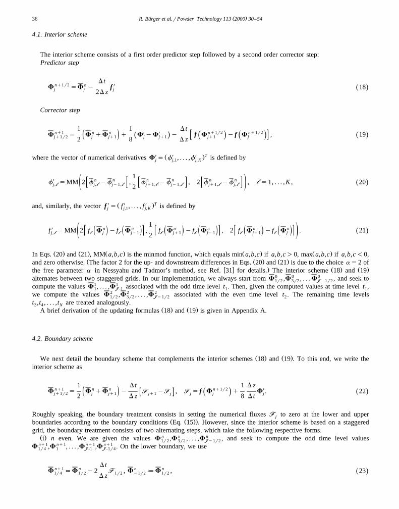
The interior scheme consists of a first order predictor step followed by a second order corrector step:Predictor step

D tXnq1r2 nF sF y f 18Ž .j j j2D z

Corrector step

1 1 D tX Xnq1 n n nq1r2 nq1r2F s F qF q F yF y f F y f F , 19Ž .Ž . Ž . Ž .ž /jq1r2 j jq1 j jq1 jq1 j2 8 D z

X Ž X X .Twhere the vector of numerical derivatives F s f , . . . ,f is defined byj j,1 j, K

1X n n n n n nf sMM 2 f yf , f yf , 2 f yf , lls1, . . . , K , 20Ž .j , ll j , ll jy1, ll jq1, ll jy1, ll jq1, ll j , llž /2

X Ž X X .Tand, similarly, the vector f s f , . . . , f is defined byj j,1 j, K

1X n n n n n nf sMM 2 f F y f F , f F y f F , 2 f F y f F . 21Ž .ž / ž / ž / ž / ž / ž /j , ll ll j ll jy1 ll jq1 ll jy1 ll jq1 ll jž /2

Ž . Ž . Ž . Ž . Ž .In Eqs. 20 and 21 , MM a,b,c is the minmod function, which equals min a,b,c if a,b,c)0, max a,b,c if a,b,c-0,Ž Ž . Ž .and zero otherwise. The factor 2 for the up- and downstream differences in Eqs. 20 and 21 is due to the choice as2 of

w x . Ž . Ž .the free parameter a in Nessyahu and Tadmor’s method, see Ref. 31 for details. The interior scheme 18 and 190 0 0alternates between two staggered grids. In our implementation, we always start from F ,F , . . . F , and seek to1r2 3r2 JJy1r2

1 1compute the values F , . . . ,F associated with the odd time level t . Then, given the computed values at time level t ,1 JJ -1 1 12 2 2we compute the values F ,F , . . . ,F associated with the even time level t . The remaining time levels1r2 3r2 JJy1r2 2

t ,t , . . . ,t are treated analogously.3 4 NŽ . Ž .A brief derivation of the updating formulas 18 and 19 is given in Appendix A.

4.2. Boundary scheme

Ž . Ž .We next detail the boundary scheme that complements the interior schemes 18 and 19 . To this end, we write theinterior scheme as

1 D t 1 D zXnq1 n n nq1r2F s F qF y FF yFF , FF s f F q F . 22Ž .Ž .ž /jq1r2 j jq1 jq1 j j j j2 D z 8 D t

Roughly speaking, the boundary treatment consists in setting the numerical fluxes FF to zero at the lower and upperjŽ Ž ..boundaries according to the boundary conditions Eq. 15 . However, since the interior scheme is based on a staggered

grid, the boundary treatment consists of two alternating steps, which take the following respective forms.n n nŽ .i n even. We are given the values F ,F , . . . ,F , and seek to compute the odd time level values1r2 3r2 JJy1r2

nq1 nq1 nq1 nq1F ,F , . . . ,F ,F . On the lower boundary, we use1r4 1 JJ -1 JJ -1r4

D tnq1 n n nF sF y2 FF , F [F , 23Ž .1r4 1r2 1r2 y1r2 1r2

D z


nwhere the auxiliary value F is used in computing the numerical flux FF . In other words, we use one-sided-1r2 1r2

differences to calculate the numerical derivatives at zsz . On the upper boundary, we use1r2

D tnq1 n n nF sF q2 FF , F [F , 24Ž .JJy1r4 JJy1r2 JJy1r2 JJq1r2 JJy1r2

D znwhere the auxiliary value F is used in computing FF . In particular, this means that we use one-sided differencesJJq1r2 JJy1r2

when computing numerical derivatives at zsz .JJy1r2n n n n nq1 nq1 nq1Ž .ii n odd. We are given the values F , F , . . . ,F ,F , and seek to compute the values F ,F , . . . ,F .1r4 1 JJ -1 JJy1r4 1r2 3r2 JJ -1r2

On the lower boundary, we use

1 D tnq1 n n n nF s F qF y FF , F [F , 25Ž .Ž .1r2 0 1 1 0 1r42 D z

nwhere the extrapolated value F is used also in computing the numerical flux FF . On the upper boundary, we use0 1

1 D tnq1 n n n nF s F qF q FF , F [F , 26Ž .Ž .JJy1r2 JJy1 JJ JJy1 JJ JJy1r42 D z

nwhere the extrapolated value F is used also in computing the numerical flux FF . A brief derivation of the updatingJJ JJy1Ž . Ž .formulas 23 – 26 is given in Appendix A.

It is a well accepted practice to utilize conservative methods when solving numerically systems of conservation lawsw x24 . Shock waves are the solution features that require this treatment. It is well known that if a conservative methodconverges, it does so to a weak solution of the conservation law. Moreover, if the scheme also satisfies a discrete entropyprinciple, the converged solution is the physical weak solution. We emphasize that the second-order predictor–corrector

Ž . Ž .Fig. 1. Settling of a bidisperse suspension of heavy particles of two different sizes: iso-concentration lines a of the larger particles and b of the smallerparticles, corresponding to the values of f s0.02, 0.04, 0.06, 0.08, 0.1, 0.15, 0.25, 0.3, 0.4, 0.5 and 0.6. The circles and the dashed lines correspond toi

w xexperimental measurements of interface locations and shock lines, respectively, obtained by Schneider et al. 26 . Concentration profiles taken at the timest , t and t are given in Fig. 2.1 2 3


w xscheme of Nessyahu and Tadmor 31 is conservative and that it also satisfies a discrete entropy principle and, thus,produces physically correct solutions.

5. Numerical simulations

In the following, we first present numerical simulations of published experimental data of the settling of polydispersesuspensions, and then simulate sedimentation of polydisperse suspensions in some hypothetical configurations exhibitinginteresting settling behaviour. The spatial discretization parameter used was D zsLr800; the time step was chosen by

< <D ts0.45D zr max r , 27Ž .ì ji , j

Ž .where r is given by Eq. 11 . The coefficient 0.45 yields a slight underestimate of the maximally admissible time step forì jŽ .the staggered grid given by replacing 0.45 in Eq. 27 by 0.5.

5.1. Comparison with published results

5.1.1. Settling of a bidisperse suspensionw x 3Consider the experiment performed by Schneider et al. 26 with glass beads of the same density D s2790 kgrm ands

of the diameters d s0.496 and d s0.125 mm in a settling column of height Ls0.3 m. The fluid density and viscosity1 2

are D s1208 kgrm3 and m s0.02416 kg my1 sy1, respectively. The initial concentrations are f 0 s0.2 and f 0 s0.05,f f 1 2w xand the simulated time here is Ts1200 s. Following Schneider et al. 26 , we employ Richardson and Zaki’s flux density

Ž . w xfunction given in Eq. 8 with ns2.7, which is cut at f s0.68, see Concha et al. 22 .max

Fig. 1 displays the simulated iso-concentration lines for each species, together with the experimental measurements ofinterface locations and computed shock lines made by Schneider et al., while Fig. 2 shows concentration profiles of bothspecies at three selected times.

w x w xFollowing Gaudin and Fuerstenau 39 and Tiller et al. 40 , we construct ‘Lagrangian paths’ to follow given sets ofparticles of each species. Integrating the concentration data at a given time with respect to height yields the heights underwhich 1%, 10%, 20%, . . . , 90% and 99% of the total mass of the particle species are located. The succession of these

Ž . Ž .Fig. 2. Settling of a bidisperse suspension of heavy particles of two different sizes: concentration profiles a of the larger particles and b of the smallerŽ .particles index 2 at t s51.9 s, t s299.8 s and t s599.7 s.1 2 3


Ž .Fig. 3. Settling of a bidisperse suspension of heavy particles of two different sizes: particle trajectories of the larger particles solid lines and of the smallerŽ .particles dashdotted lines . Concentration profiles taken at the times t , t and t are given in Fig. 2.1 2 3

points with respect to time yields curves that may be considered as trajectories of particles initially separated by 1% fromŽ .the remaining 99% and so on of total mass of that species. With the exception of the 1% line of the heavy particles, the

particle trajectories computed from the concentration data of Fig. 1 are shown in Fig. 3. Fig. 1 shows a good agreement ofsimulated and experimental results, and Fig. 3 shows clearly that the small particles have initially an upward constantmovement before settling at constant rate as if they were alone in the suspension.

w x w xIn addition to the original initial data used by Schneider et al. 26 , Concha et al. 22 considered also a hypotheticalsettling experiment of the same bidisperse suspension with the considerably increased initial concentrations f 0 s0.35 and1

f 0 s0.05. The simulated time is again Ts1200 s.2

Ž . Ž .Fig. 4. Settling of a bidisperse suspension of heavy particles of two different sizes: iso-concentration lines a of the larger particles and b of the smallerparticles, corresponding to the values of f s0.02, 0.032, 0.038, 0.04, 0.042, 0.044, 0.046, 0.048, 0.06, 0.08, 0.1, 0.12, 0.14, 0.16, 0.18, 0.2, 0.25, 0.3, 0.4,i

0.5, 0.6 and 0.65. Concentration profiles taken at the times t , t and t are given in Fig. 5. In Fig. 6, the upper left quarter of the settling plot for the1 2 3w xsmaller particles is shown together with relevant parts of numerical results from Ref. 22 .


Ž . Ž .Fig. 5. Settling of a bidisperse suspension of heavy particles of two different sizes: concentration profiles a of the larger particles and b of the smallerŽ .particles index 2 at t s168.2 s, t s302.7 s and t s598.7 s.1 2 3

The numerical results are shown in Figs. 4 and 5. Fig. 6 shows that our numerical results for this problem differ in somew x w xregions significantly from the results in Ref. 22 , which were computed by a finite difference algorithm due to Lee 41 . In

particular, we believe that the strange behaviour of the interface between clear liquid and suspension, marked by the fatw xdashed line in Fig. 6, might be due to an error in Lee’s rather complicated interface tracking algorithm 41 .

5.1.2. Separation of a bidisperse suspension with light and heaÕy particlesw x w xFessas and Weiland 42,43 and Weiland and MacPherson 44 studied the increase of settling rates of a given

monodisperse suspension of heavy particles if lighter, buoyant particles are added. This phenomenon has been studied byw xLaw et al. 21 as a comparison example for several of the mathematical models for polydisperse suspensions reviewed in

Ž . w xFig. 6. Detail of Fig. 4 b . In addition, some iso-concentration lines for the smaller particles computed by Concha et al. 22 are shown.


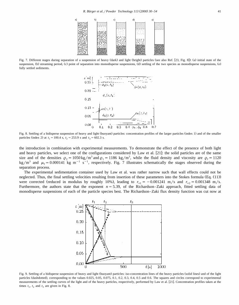
Ž . Ž . Ž w x. Ž .Fig. 7. Different stages during separation of a suspension of heavy dark and light bright particles see also Ref. 23, Fig. 8 : a initial state of theŽ . Ž . Ž . Ž .suspension, b streaming period, c point of separation into monodisperse suspensions, d settling of the two species as monodisperse suspensions, e

fully settled sediments.

Ž . Ž .Fig. 8. Settling of a bidisperse suspension of heavy and light buoyant particles: concentration profiles of the larger particles index 1 and of the smallerŽ .particles index 2 at t s100.4 s, t s253.9 s and t s602.3 s.1 2 3

the introduction in combination with experimental measurements. To demonstrate the effect of the presence of both lightw xand heavy particles, we select one of the configurations considered by Law et al. 21 : the solid particles are of the same

size and of the densities D s1050 kgrm3 and D s1186 kgrm3, while the fluid density and viscosity are D s11202 1 f

kgrm3 and m s0.000141 kg my1 sy1, respectively. Fig. 7 illustrates schematically the stages observed during thef

separation process.The experimental sedimentation container used by Law et al. was rather narrow such that wall effects could not be

Ž Ž ..neglected. Thus, the final settling velocities resulting from insertion of these parameters into the Stokes formula Eq. 11Ž .were corrected reduced in modulus by roughly 10% , leading to r sy0.001241 mrs and r s0.001348 mrs.`1 `2

Furthermore, the authors state that the exponent ns5.39, of the Richardson–Zaki approach, fitted settling data ofmonodisperse suspensions of each of the particle species best. The Richardson–Zaki flux density function was cut now at

Ž . Ž .Fig. 9. Settling of a bidisperse suspension of heavy and light buoyant particles: iso-concentration lines of the heavy particles solid lines and of the lightŽ .particles dashdotted , corresponding to the values 0.025, 0.05, 0.075, 0.1, 0.2, 0.3, 0.4, 0.5 and 0.6. The squares and circles correspond to experimental

w xmeasurements of the settling curves of the light and of the heavy particles, respectively, performed by Law et al. 21 . Concentration profiles taken at thetimes t , t and t are given in Fig. 8.1 2 3


Ž . Ž .Fig. 10. Settling of a bidisperse suspension of heavy and light buoyant particles: particle trajectories of the heavy solid lines and of the light particlesŽ .dashdotted lines . Concentration profiles taken at the times t , t and t are given in Fig. 8.1 2 3

Ž . Ž .Fig. 11. Settling of a bidisperse suspension of heavy and light buoyant particles: iso-concentration lines of the heavy particles solid lines and of the lightŽ .particles dashdotted , corresponding to the values 0.025, 0.05, 0.075, 0.1, 0.15, 0.2, 0.3, 0.4, 0.5 and 0.6. Concentration profiles taken at the times t , t1 2

and t are given in Fig. 13.3

f s0.6713. In the experiment simulated here, the suspension was of initial height 0.283 m and contained initially 8% ofmax

each solid species.w xIn Ref. 21 , only the intersecting interface curves of both species are displayed for tQ320 s; here, the complete

separation process is shown for tFTs1000 s. Fig. 8 shows concentration profiles for both species at three selected times,ŽFig. 9 shows the iso-concentration lines for both species the qualitatively different behaviour of both species makes it

.possible to collect the respective settling plots into one diagram , and Fig. 10 presents the particle trajectories, which wereobtained in the same way as in the previous example.

Ž . Ž .Fig. 12. Settling of a bidisperse suspension of heavy and light buoyant particles: particle trajectories of the heavy solid lines and of the light particlesŽ .dashdotted lines . Concentration profiles taken at the times t , t and t are given in Fig. 13.1 2 3


Ž . Ž .Fig. 13. Settling of a bidisperse suspension of heavy and light buoyant particles: concentration profiles of the larger particles index 1 and of the smallerŽ .particles index 2 at t s301.1 s, t s501.9 s and t s897.5 s.1 2 3

The results illustrate that the numerical scheme predicts correctly the expected separation behaviour. Fig. 9 indicates thatboth phases are already entirely separated at ts t , and that the final state of the suspension consists of two sediments of2

maximum solids concentration separated by clear liquid.w x 0 0We also simulate a second experiment performed by Law et al. 21 ; namely, we take f s0.20 and f s0.15, and1 2

leave the remaining parameters unchanged. The corresponding numerical results are given in Figs. 11, 12 and 13.By the behaviour of the iso-concentration lines corresponding to f s0.5, f s0.6 and f s0.6 and by the shapes of1 1 2

the ‘edges’ of the sediment layers forming at the top and at the bottom of the column, respectively, these results make the

Ž . Ž .Fig. 14. Settling of a suspension of heavy particles of four different sizes: iso-concentration lines of a the largest, b the second largest particles,corresponding to the values 0.005, 0.03, 0.055, 0.08, 0.1, 0.15, 0.2, 0.25, 0.3, 0.4, 0.5 and 0.6. The dashed lines correspond to kinematic shock lines

w xcalculated by Greenspan and Ungarish 27 . The concentration profiles at time t are included in Fig. 16.1


occurrence of rarefaction waves apparent. Moreover, Fig. 13 shows that at ts t , by its sharp edge, the upper sediment is3

already in its final state, in contrast to the lower.It should be mentioned that our numerical results differ substantially from the behaviour of this suspension observed by

w xLaw et al. 21 : their photograph clearly illustrates that at high initial concentrations in a suspension with buoyant particles,lateral segregation between heavy and light solids during separation occurs. Macroscopically, this movement becomes

Ž w x.visible as an intrinsically two-dimensional ‘fingering’ effect see Ref. 45 and is, therefore, out of the scope of thew xone-dimensional model considered here. This conclusion had also been drawn by Shih et al. 23 , who simulated a similar

experiment by a one-dimensional hydrodynamical model including compression effects.

5.1.3. Sedimentation of a suspension with particles of four different sizesw xIn Ref. 27 , Greenspan and Ungarish consider the settling of a polydisperse suspension of four different sizes. They useŽ .the function in our notation

2f

GUV f sV f [ 1y , f s0.6, 28Ž . Ž . Ž .maxž /fmax

and represent their solution in dimensionless variables. To make their result comparable with the previous calculations, weselect, as in the first example, D s2790 kgrm3, D s1208 kgrm3, m s0.02416 kg my1 sy1, Ls0.3 m and d s0.496s f f 1

mm. The smaller particles are assumed to be of the diameters d s0.8d s0.3968 mm, d s0.6 d s0.2976 mm and2 1 3 1

d s0.4 d s0.1984 mm. The constant initial concentrations are f 0 sf 0 sf 0 sf 0 s0.05. In Figs. 14 and 15, we show4 1 1 2 3 4

Ž . Ž .Fig. 15. Settling of a suspension of heavy particles of four different sizes: iso-concentration lines of a the second smallest, b the smallest particles,corresponding to the values 0.005, 0.03, 0.055, 0.08, 0.1, 0.15, 0.2, 0.25, 0.3, 0.4, 0.5 and 0.6. The dashed lines correspond to kinematic shock lines

w xcalculated by Greenspan and Ungarish 27 . The concentration profiles at time t are included in Fig. 16.1


Fig. 16. Settling of a suspension of heavy particles of four different sizes: concentration profiles of species 1 to 4 at t s615.07 s and t s2000.0 s. The1 2Ž .horizontal and vertical lines are the stationary kinematic shock solution the number i corresponds to species i, is1, . . . ,4 by Greenspan and Ungarish

w x27 . The approximation of their solution indicates which numerically calculated concentration profile calculated here belongs to which species.

the solution represented by iso-concentration lines for tFTs720 s. The particle trajectories turned out very similar tothose of Fig. 3 and are, therefore, not depicted.

w xGreenspan and Ungarish 27 determine a solution of the same problem within the class of piecewise constant functions,separated by kinematic shocks as outlined above. To make comparison possible, their solution is also drawn in Figs. 14 and15. Their result implies, in particular, that the sediment composition remains constant for all times once the discontinuityseparating the suspension in hindered settling from the clear liquid has reached the sediment level. Our numerical solutionfor a large time is compared with their result in Fig. 16.

Ž .Fig. 17. Settling of a bidisperse suspension of heavy particles of two different sizes initially located above clear liquid: iso-concentration lines a of theŽ .larger particles and b of the smaller particles, corresponding to the values of f 0.001, 0.007, 0.02, 0.04, 0.06, 0.08, 0.095, 0.099, 0.11, 0.20, 0.3, 0.4, 0.5i

and 0.6.


Fig. 18. Settling of a bidisperse suspension of heavy particles of two different sizes initially located above clear liquid: particle trajectories of the heavyŽ . Ž .solid lines and of the light particles dashdotted lines .

This example illustrates that the scheme is able to treat systems of more than two particle species. Figs. 14 and 15suggest, by the incidence with the shock lines computed by our numerical methods, that the kinematic shock construction is

Ž . Ž .in this case correct for the family of shock lines emerging from z,t s L,0 . However, the construction of a single shockŽ . Ž .emerging from z,t s 0,0 appears not to be correct, and is replaced here by a rarefaction wave, which starts to interact

Ž .earlier with the fastest downwards traveling shock see Fig. 14a . Although the transient settling process simulatednumerically is quite different from the kinematic shock construction, the results for the sediment composition given in Fig.16 for a large time are comparable. However, note that the behaviour of the profiles of f and f below the respective3 4

zones where these concentrations are dominant suggest that continuous transitions also have to be considered as part ofsteady state solutions.

5.2. Hypothetical test cases

5.2.1. Rarefaction waÕes in a bidisperse suspensionThe preceding examples illustrate what is well known from the theory of monodisperse ideal suspensions: sediment is

not only composed by kinematic shocks and their interactions; rather, the effect of rarefaction waves has to be taken intoaccount. We present now two examples imposing initial conditions which, in view of comparable results known from thesedimentation behaviour of monodisperse suspensions, can be expected to produce rarefaction waves.

In the first case, consider a ‘membrane problem’: we assume that the upper half of the settling column is initially filledwith a bidisperse suspension, while its lower half contains pure liquid:

0.1 for zG0.15 m,0 0f z sf z sŽ . Ž .1 2 ½ 0 for z-0.15 m.

w xThe remaining parameters are identical to the data used by Schneider et al. 26 . The simulated time is Ts900 s. Theresults are given in Figs. 17 and 18. Note that the spreading of the trajectories of the smaller particles visible in Fig. 18corresponds to the formation of a rarefaction wave.

Fig. 19. Settling of a bidisperse suspension of heavy particles of two different sizes with piecewise monodisperse initial states: particle trajectories of theŽ . Ž .larger particles solid lines and of the smaller particles dashdotted lines .


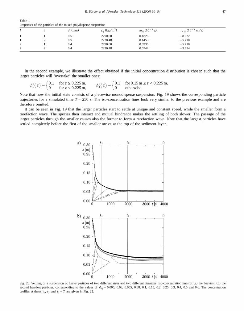
Table 1Properties of the particles of the mixed polydisperse suspension

3 y3 y3Ž . Ž . Ž . Ž .I j d mm D kgrm m 10 g r 10 mrsi j i j ` i j

1 1 0.5 2790.00 0.1826 y8.9221 2 0.5 2220.48 0.1453 y5.7102 1 0.4 2790.00 0.0935 y5.7102 2 0.4 2220.48 0.0744 y3.654

In the second example, we illustrate the effect obtained if the initial concentration distribution is chosen such that thelarger particles will ‘overtake’ the smaller ones:

0.1 for zG0.225 m, 0.1 for 0.15 mFz-0.225 m,0 0f z s f z sŽ . Ž .1 2½ ½0 for z-0.225 m, 0 otherwise.

Note that now the initial state consists of a piecewise monodisperse suspension. Fig. 19 shows the corresponding particletrajectories for a simulated time Ts250 s. The iso-concentration lines look very similar to the previous example and aretherefore omitted.

It can be seen in Fig. 19 that the larger particles start to settle at unique and constant speed, while the smaller form ararefaction wave. The species then interact and mutual hindrance makes the settling of both slower. The passage of thelarger particles through the smaller causes also the former to form a rarefaction wave. Note that the largest particles havesettled completely before the first of the smaller arrive at the top of the sediment layer.

Ž . Ž .Fig. 20. Settling of a suspension of heavy particles of two different sizes and two different densities: iso-concentration lines of a the heaviest, b thesecond heaviest particles, corresponding to the values of f s0.005, 0.03, 0.055, 0.08, 0.1, 0.15, 0.2, 0.25, 0.3, 0.4, 0.5 and 0.6. The concentrationi j

profiles at times t , t and t sT are given in Fig. 22.1 2 3


5.2.2. Settling of a mixed polydisperse suspension with different particle sizes and different densitiesSo far, we have considered only mixtures in which the particle species differ either in size or in density. However, the

model equations permit that particles differ in both properties. To demonstrate the effects occurring in such a system, weŽ .chose an example of four different particle species NsMs2 having the properties given in Table 1, where m denotesi j

the mass of species ij. The relevant properties of the fluid are again D s1208 kgrm3 and m s0.02416 kg my1 sy1.f f

The parameters have been selected such that all four species have different particle mass while the second and thirdheaviest species possess equal final settling velocity. A classical experiment with one pair of particle species differing in

w x Žsize and density, but having the same final settling velocity, was conducted by Richardson and Meikle 46 see also Refs.w x. Ž Ž .. w x19,47 . In this case, we employed the drag law Eq. 16 proposed by Barton et al. 38 , whose parameters f s0.6,max

ns5 and ls5r59 have been adopted. The Kynch flux density function corresponding to this choice possesses twoXŽ .inflection points and satisfies f f )0. Consequently, any rarefaction wave emerging from zs0, ts0 will be finite,max

i.e., it does not contain characteristics of infinitely small slope, in contrast to what happens if the Richardson–Zaki drag lawis used without cutting it at a maximum concentration f -1. This means that the batch sedimentation process shouldmax

terminate after finite time.The numerical solution of this example is depicted in Figs. 20–23. Calculations were performed for a simulated time of

Ts4000 s. Indeed, all iso-concentration lines become horizontal. Unfortunately, severe diffusion somewhat distorts theresults. This becomes evident by the spreading of close-by iso-concentration lines, which are meant to denote a kinematicshock of the exact solution.

The main reason for this undesirable effect is the coexistence of physical phenomena within the sedimentation modelwhich propagate both at very small and at large velocities. That is, some of the concentrations quickly tend to developstationary or almost stationary shocks, while this takes much longer time for others. With explicit schemes as the oneemployed here, however, the time step is limited by the fastest moving concentration component. Consequently, explicitschemes limit the time step to a much smaller value than is actually sufficient to accurately resolve the transient behaviour

Ž . Ž .Fig. 21. Settling of a suspension of heavy particles of two different sizes and two different densities: iso-concentration lines of a the second lightest, bthe lightest particles, corresponding to the values of f s0.005, 0.03, 0.055, 0.08, 0.1, 0.15, 0.2, 0.25, 0.3, 0.4, 0.5 and 0.6. The concentration profiles ati j

times t , t and t sT are given in Fig. 22.1 2 3


Ž . Ž .Fig. 22. Settling of a suspension of heavy particles of two different sizes and two different densities: concentration profiles of a the heaviest and b thesecond heaviest particles at t s499.3 s, t s1997.4 s and t sT s4000.1 2 3

Ž .Fig. 23. Settling of a suspension of heavy particles of two different sizes and two different densities: concentration profiles of a the second lightest andŽ .b the lightest particles at t s499.3 s, t s1997.4 s and t sT s4000.1 2 3


of the slowly moving components. For the particular scheme used here, this becomes apparent by the excessive diffusion inthe concentration isolines corresponding to the lightest or smallest particle species when performing long time integration. Adetailed study of this phenomenon produced by the numerical scheme and possible strategies for its correction are presented

w xin Ref. 30 .

6. Conclusions

We have shown that the use of modern shock-capturing schemes represents a serious alternative to the shock-trackingtechniques that have been proposed for the simulation of settling of polydisperse suspensions. This is illustrated by theagreement with experimental data and the fact that there are no principal problems in treating large numbers of particlespecies. Moreover, these schemes obey an entropy principle and therefore approximate the unique physically relevantsolution. This becomes apparent by several test cases in which the scheme replaces a constructed kinematic shock by ararefaction wave.

The scheme used in this paper is a high-resolution scheme which is particularly easy to implement. For completeness, theŽ .few necessary formulas for implementing the scheme have been included in this paper. It is also possible to consider otherschemes. A comparative study of some modern shock-capturing schemes for simulating the settling of polydisperse

w xsuspensions is presented in Ref. 30 .We suggest employing these schemes for the study of several additional problems that could not be considered here, for

w xexample, for the study of fluidization problems such as bed inversion 48 , for the testing of Davis and Gecol’s neww xparameterless hindered settling function 36 , as these authors suggest, for tridisperse and more complex suspensions, and

for the simulation of the transient behaviour of polydisperse suspensions in mineral processing applications, such as densityw xseparation 49 . On the other hand, the severe limitations of kinematic sedimentation models have become evident for

monodisperse suspensions, since most industrial slurries develop compressible sediments, which a kinematic theory cannotw xdescribe. Therefore the rigorous phenomenological model developed for monodisperse flocculated suspensions 50 should

w xbe extended to polydisperse mixtures, following, for example, Stamatakis and Tien 51 . Also for such models it should bepossible to apply shock-capturing schemes, following, e.g., the splitting approach implemented in the monodisperse case by

w xBustos et al. 5 .

7. List of symbols

d diameter of particle species ijiŽ .f f Kynch batch flux density functionŽ .f F flux density function for particle species iji j

f flux density vectorf X approximate derivative used by numerical schemej

FF numerical fluxj

g acceleration of gravityj space step index used by numerical schemeJJ number of space intervalsK assumed number of particle speciesL height of the settling columnM number of different particle densities

Ž .MM P,P,P minmod function used by numerical schemen exponent in drag law formulasn time step index used by numerical schemeN number of different particle diametersNN number of time intervalsq volume average velocityr relative velocity between particle species ij and the fluidi j

r Stokes settling velocity of a single particle of species ijì j

t timet discrete timen

T endpoint of simulated time intervalÕ local velocity of the fluidf


Õ phase velocity of particle species iji j

Õ solids phase velocitysŽ .V f drag law or hindered settling function

z heightz discrete heightj

Greek lettersa parameter in Nessyahu and Tadmor’s methodd ratio d2rd 2

i i 1

D t, D z discretization parametersl parameter in Barton et al.’s formulam a parameter in the definition of fi j

m viscosity of the fluidf

f solids total volume fractionf homogeneous initial concentration of a monodisperse suspension0

Ž .f z initial concentration distribution of a monodisperse suspension0

f volumetric concentration of particle species iji j0 Ž .f z initial distribution of fi j i j

f maximum concentrationmaxŽ .F z,t numerical approximationnnF cell average used by numerical schemejnq1F auxiliary values used by the boundary schemey1r2,1r4, JJy1r4, JJq1r2

F nq1r2 predictor value used by numerical schemejnq1F corrector value used by numerical schemejq1r2

FX approximate derivative used by numerical schemej

F matrix of concentration values fi j

D fluid densityf

D density of particle species ijj

D solids densitys

s jump propagation velocityi j

Acknowledgements

KKF and KHK are grateful to the group of Prof. Dr.-Ing. Dr. H.C.W.L. Wendland at the Institute of Mathematics A,University of Stuttgart, for hospitality. The preparation of this paper was made possible by travel grants awarded by the

Ž . Ž .European Science Foundation ESF through the Applied Mathematics in Industrial Flow Problems AMIF programme.Support by the Sonderforschungsbereich 404 at the University of Stuttgart is also gratefully acknowledged. We alsoacknowledge support of Fondef project D97-I2042.

Appendix A. Brief derivation of the numerical scheme

In this appendix, we briefly derive the difference formulas introduced in Section 4. As mentioned in Section 4, we divideŽ . Ž . Ž . Ž .the description of the scheme into an interior part, i.e., formulas 18 and 19 , and a boundary part, i.e., formulas 23 – 26 .

A.1. Interior scheme

n� 4 Ž .At time level t , given the cell averages F see below , we introduce a piecewise linear approximate solutionn j jŽ .F z,t of the formn

1Xn w xF z ,t sF q F zyz for zg z , z , 29Ž . Ž . Ž .n j j j jy1r2 jq1r2

D z


X Ž X .T Ž . Žwhere F s f c, . . . ,f is the slope vector defined in Eq. 20 . In particular, this choice of slope vector satisfies seej j,1 j, Kw x.Ref. 31

1 EXF s F zsz ,t qOO D z ,Ž .Ž .j j n

D z Ez

which ensures second-order accuracy wherever the components of F are smooth. In addition, this choice ensures that thew xapproximation is non-oscillatory. We refer to Ref. 31 for other choices of slope vectors. Now integrating the conservation

laws

E EFq f F s0 30Ž . Ž .

Et Ez

w x w xover z , z = t ,t yields the following exact evolution equation of F:j jq1 n nq1

1 t tnq1 nq1nq1 nF sF y f F z ,t d ty f F z ,t d t , 31Ž .Ž . Ž .Ž . Ž .H Hjq1r2 jq1r2 jq1 jy1D z t tn n

nwhere F is the cell average defined byjq1r2

z1 jq1nF s F z ,t d z , 32Ž . Ž .Hjq1r2 nD z zj

nq1 Ž .and similarly for F . Note that explicit expressions for the integral averages given by Eq. 32 can be deduced easilyjq1r2Ž .from Eq. 29 . In fact,

1 1X Xn n nF s F qF q F yF .Ž .ž /jq1r2 j jq1 j jq12 8

Ž . ŽFor a sufficiently small time step D t, the time integrals in Eq. 31 only involve smooth integrands due to the. Ž w x.staggering so that they can be computed within any degree of accuracy by an appropriate quadrature rule see Ref. 31 .

Here, the time integrals of the flux are approximated by the second-order accurate mid-point rule,

1 D ttnq1 f F z ,t d tf f F z ,t ,Ž . Ž .Ž . Ž .H j j nq1r2D z D ztn

where the point-values at the half time steps are evaluated by Taylor expansion,

D t E D tXnq1r2 nF [F z ,t fF z ,t q F z ,ts t sF y f . 33Ž .Ž . Ž . Ž .j j nq1r2 j n j n j j2 Et 2D z

X Ž X X .T Ž .Here, the slope vector f s f , . . . , f is defined in Eq. 21 . In particular, this choice of slope vector ensuresj j,1 j, K

second-order accuracy in smooth regions, i.e.,

1 EXf s f F zsz ,t qOO D z ,Ž .Ž .Ž .j j n

D z Ez

Ž w x.and that the numerical approximation is non-oscillatory see Ref. 31 . Summing up, we end up with the interior schemeŽ . Ž . w x18 and 19 . We refer to Nessyahu and Tadmor 31 for further details on the derivation of the interior scheme.

A.2. Boundary scheme

Ž . Ž . Ž .We next derive the formulas 23 – 26 , i.e., the boundary scheme. Let us first derive Eq. 23 , where the auxiliary valuenq1 Ž . w xF denotes the average of F z, t on the boundary half-cell z , z centred on z ,1r4 nq1 0 1r2 1r4

z2 1r2nq1F s F z ,t d z .Ž .H1r4 nq1D z z0

w xThe concept of boundary half-cells was introduced by Levy and Tadmor 52 in their treatment of Dirichlet boundaryw xconditions for the Nessyahu and Tadmor scheme 31 . We emphasize that the boundary scheme used in this paper is not

w xderived in Refs. 31,52 .


Ž Ž .. w x w xIntegrating the conservation law Eq. 30 over z , z = t ,t and taking into account that the physical flux0 1r2 n nq1Ž .should, according to Eq. 15 , vanish at zsz , we get0

2 tnq1nq1 nF sF y f F z ,t d t . 34Ž .Ž .Ž .Hjq1r4 jq1r4 1r2D z tn

Ž .Using Eq. 29 with js1r2, a straightforward computation reveals that

z2 11r2 Xn nF [ F z ,t d zsF y F .Ž .H1r4 n 1r2 1r2D z 4z0

Ž .Using this and the mid-point rule to replace the time integral in Eq. 34 , we obtain

1 D tXnq1 n nq1r2F sF y F y2 f F ,Ž .1r4 1r2 1r2 1r24 D z

Ž Ž .. nq1r2 Ž .which is precisely Eq. 23 if we identify the predictor value F as Eq. 33 with js1r2. This predictor value1r2n nbecomes well-defined once we introduce the auxiliary value F :sF . In other words, we use one-sided differencesy1r2 1r2

n nq1to calculate the numerical derivatives at zsz . Defining the auxiliary values F and F as the averages on the1r2 JJy1r4 JJy1r4w x Ž . Ž Ž ..boundary half-cell z , z of F z,t at ts t and ts t , respectively, the formula Eq. 24 for the upperJJy1r2 JJ n nq1

boundary can be derived similarly.Ž . Ž Ž ..Let us now derive Eq. 25 . Using the updating formula Eq. 22 with js0, we get

1 D tnq1 n n w xF s F qF y FF yFF ,Ž .1r2 0 1 1 02 D z

n n Ž . Ž Ž ..where F :sF . Now Eq. 25 is obtained by simply setting FF :s0. The formula Eq. 26 for the upper boundary is0 1r4 0

obtained similarly.This concludes the discussion of the boundary scheme.

References

w x1 R. Aris, N.R. Amundson, Mathematical Methods in Chemical Engineering, First-Order Partial Differential Equations with Applications Vol. 2:Prentice-Hall, Englewood Cliffs, NJ, USA, 1973.

w x Ž .2 M.C. Bustos, F. Concha, Kynch theory of sedimentation, in: E. Tory Ed. , Sedimentation of Small Particles in a Viscous Fluid, ComputationalMechanics Publications, Southampton, UK, 1996, pp. 7–49, Chap. 2.

w x Ž .3 G.J. Kynch, A theory of sedimentation, Trans. Faraday Soc. 48 1952 166–176.w x Ž .4 M.C. Bustos, F. Concha, On the construction of global weak solutions in the Kynch theory of sedimentation, Math. Meth. Appl. Sci. 10 1988

245–264.w x5 M.C. Bustos, F. Concha, R. Burger, E.M. Tory, Sedimentation and Thickening: Phenomenological Foundation and Mathematical Theory, Kluwer¨

Academic Publishers, Dordrecht, Netherlands, 1999.w x6 M.C. Bustos, F. Concha, W.L. Wendland, Global weak solutions to the problem of continuous sedimentation of an ideal suspension, Math. Meth.

Ž .Appl. Sci. 13 1990 1–22.w x Ž .7 S. Diehl, A conservation law with point source and discontinuous flux function modelling continuous sedimentation, SIAM J. Appl. Math. 56 1996

388–419.w x Ž .8 S. Diehl, Dynamic and steady-state behaviour of continuous sedimentation, SIAM J. Appl. Math. 57 1997 991–1018.w x Ž .9 S. Diehl, Continuous sedimentation of multi-component particles, Math. Meth. Appl. Sci. 20 1997 1345–1364.

w x Ž .10 C.A. Petty, Continuous sedimentation of a suspension with nonconvex flux law, Chem. Eng. Sci. 30 1975 1451–1458.w x Ž .11 R. Burger, W.L. Wendland, F. Concha, Model equations for gravitational sedimentation–consolidation processes, Z. Angew. Math. Mech. 80 2000¨

79–92.w x12 R. Burger, M.C. Bustos, F. Concha, Settling velocities of particulate systems: 9. Phenomenological theory of sedimentation processes: numerical¨

Ž .simulation of the transient behaviour of flocculated suspensions in an ideal batch or continuous thickener, Int. J. Miner. Process. 55 1999 267–282.w x Ž .13 R. Burger, F. Concha, Mathematical model and numerical simulation of the settling of flocculated suspensions, Int. J. Multiphase Flow 24 1998¨

1005–1023.w x Ž .14 T.N. Smith, The differential sedimentation of particles of two different sizes, Trans. Inst. Chem. Eng. 43 1965 T69–T73.w x Ž .15 T.N. Smith, The sedimentation of particles having a dispersion of sizes, Trans. Inst. Chem. Eng. 44 1966 T152–T157.w x Ž .16 M.J. Lockett, H.M. Al-Habbooby, Differential settling by size of two particles in a liquid, Trans. Inst. Chem. Eng. 51 1973 281–292.w x Ž .17 M.J. Lockett, H.M. Al-Habbooby, Relative particle velocities in two-species settling, Powder Technol. 10 1974 67–71.w x Ž .18 S. Mirza, J.F. Richardson, Sedimentation of suspensions of particles of two or more sizes, Chem. Eng. Sci. 34 1979 447–454.w x Ž .19 J.H. Masliyah, Hindered settling in a multiple-species particle system, Chem. Eng. Sci. 34 1979 1166–1168.w x Ž .20 V.S. Patwardhan, C. Tien, Sedimentation and liquid fluidization of solid particles of different sizes and densities, Chem. Eng. Sci. 40 1985

1051–1060.w x21 H.S. Law, J.H. Masliyah, R.S. MacTaggart, K. Nandakumar, Gravity separation of bidisperse suspensions: light and heavy particle species, Chem.

Ž .Eng. Sci. 42 1987 1527–1538.


w x22 F. Concha, C.H. Lee, L.G. Austin, Settling velocities of particulate systems: 8. Batch sedimentation of polydisperse suspensions of spheres, Int. J.Ž .Miner. Process. 35 1992 159–175.

w x Ž .23 Y.T. Shih, D. Gidaspow, D.T. Wasan, Hydrodynamics of sedimentation of multisized particles, Powder Technol. 50 1987 201–215.w x24 R.J. Le Veque, Numerical Methods for Conservation Laws, 2nd edn., Birkhauser, Basel, 1992.¨w x Ž .25 A. Kluwick, Kinematische Wellen, Acta Mech. 26 1977 15–46.w x Ž .26 W. Schneider, G. Anestis, U. Schaflinger, Sediment composition due to settling of particles of different sizes, Int. J. Multiphase Flow 11 1985

419–423.w x Ž .27 H.P. Greenspan, M. Ungarish, On hindered settling of particles of different sizes, Int. J. Multiphase Flow 8 1982 587–604.w x Ž .28 M.S. Selim, A.C. Kothari, R.M. Turian, Sedimentation of multisized particles in concentrated suspensions, AIChE J. 29 1983 1029–1038.w x Ž .29 K. Stamatakis, C. Tien, Dynamics of batch sedimentation of polydispersed suspensions, Powder Technol. 56 1988 105–117.w x30 R. Burger, K.-K. Fjelde, K.H. Karlsen, Numerical methods for systems of conservation laws modelling sedimentation of polydisperse suspensions, in¨

preparation.w x Ž .31 H. Nessyahu, E. Tadmor, Non-oscillatory central differencing for hyperbolic conservation laws, J. Comp. Phys. 87 1990 408–463.w x32 W.Z. Choi, G.T. Adel, R.H. Yoon, Size reductionrliberation model of grinding including multiple classes of composite particles, Miner. Metall.

Ž .Process. 1987 102–108, May.w x33 H.J. Steiner, Liberation kinetics in grinding operations,Proc. of the XI International Mineral Processing Congress, Cagliari, Italy, 1975, pp. B1–B26.w x Ž .34 I.S. Zaidenberg, D.I. Sisovski, I.A. Burova, A form of construction of a mathematical model of the flotation process, Tsvetn. Metal. 37 1964 24–30.w x Ž . Ž .35 J.F. Richardson, W.N. Zaki, Sedimentation and fluidization I, Trans. Inst. Chem. Eng. London 32 1954 35–53.w x Ž .36 R.H. Davis, H. Gecol, Hindered settling function with no empirical parameters for polydisperse suspensions, AIChE J. 40 1994 570–575.w x37 G.B. Wallis, One-dimensional Two-phase Flow, McGraw-Hill, New York, 1969.w x Ž .38 N.G. Barton, C.H. Li, S.J. Spencer, Control of a surface of discontinuity in continuous thickeners, J. Aust. Math. Soc. Ser. B 33 1992 269–280.w x Ž .39 A.M. Gaudin, M.C. Fuerstenau, Experimental and mathematical model of thickening, Trans. AIME 223 1962 122–129.w x40 F.M. Tiller, N.B. Hsyung, Y.L. Shen, CATSCAN analysis of sedimentation and constant pressure filtration, Proc. of the V World Filtration Congress,

Societe Francaise de Filtration, Nice, France Vol. 2, 1991, pp. 80–85.´ ´w x41 C.H. Lee, Modeling of Batch Hindered Settling, PhD thesis, College of Earth and Mineral Sciences, Pennsylvania State University, University Park,

PA, USA, 1989.w x Ž .42 Y.P. Fessas, R.H. Weiland, Convective solids settling induced by a buoyant phase, AIChE J. 27 1981 588–592.w x Ž .43 Y.P. Fessas, R.H. Weiland, The settling of suspensions promoted by rigid buoyant particles, Int. J. Multiphase Flow 10 1984 485–507.w x Ž .44 R.H. Weiland, R.R. McPherson, Accelerated settling by addition of buoyant particles, Ind. Eng. Chem. Fundam. 18 1979 45–49.w x45 R.H. Weiland, Y.P. Fessas, B.V. Ramarao, On instabilities arising during sedimentation of two-component mixtures of solids, J. Fluid Mech. 142

Ž .1984 383–389.w x46 J.F. Richardson, R.A. Meikle, Sedimentation and fluidization: Part III. The sedimentation of uniform fine particles and of two-component mixtures of

Ž .solids, Trans. Inst. Chem. Eng. 39 1961 348–356.w x47 J.M. Coulson, J.F. Richardson, J.R. Backhurst, J.H. Harker, Chemical Engineering, 4th edn., Particle Technology and Separation Processes Vol. 2,

Butterworth-Heinemann, Oxford, UK, 1991.w x Ž .48 N. Epstein, B.P. Le Clair, Liquid fluidization of binary particle mixtures — II. Bed inversion, Chem. Eng. Sci. 40 1985 1517–1526.w x Ž .49 Y. Zimmels, Theory of density separation of particulate systems, Powder Technol. 43 1985 127–139.w x Ž .50 F. Concha, M.C. Bustos, A. Barrientos, Phenomenological theory of sedimentation, in: E. Tory Ed. , Sedimentation of Small Particles in a Viscous

Fluid, Computational Mechanics Publications, Southampton, UK, 1996, pp. 51–96, Chap. 3.w x Ž .51 K. Stamatakis, C. Tien, Batch sedimentation calculations — the effect of compressible sediment, Powder Technol. 72 1992 227–240.w x52 D. Levy, E. Tadmor, Non-oscillatory boundary treatment for staggered central schemes, UCLA-CAM Report 1, 1998.

Documents

Numerical simulation of the settling of polydisperse ...folk.uio.no/kennethk/articles/art18_journal.pdf · Numerical simulation of the settling of polydisperse suspensions of spheres