Embed Size (px)
Citation preview

Numerical Simulations of Giant Planetary
Core Formation
by
Henry Hoang Khoi Ngo
A thesis submitted to the Graduate Program in
the Department of Physics, Engineering Physics & Astronomy
in conformity with the requirements for the
Degree of Master of Science
Queen’s University
Kingston, Ontario, Canada
August 2012
Copyright c© Henry Hoang Khoi Ngo, 2012

Abstract
In the widely accepted core accretion model of planet formation, small rocky and/or
icy bodies (planetesimals) accrete to form protoplanetary cores. Gas giant planets are
believed to have solid cores that must reach a critical mass, ∼10 Earth masses (M⊕),
after which there is rapid inflow of gas from the gas disk. In order to accrete the
gas giants’ massive atmospheres, this step must occur within the gas disk’s lifetime
(1− 10 million years).
Numerical simulations of solid body accretion in the outer Solar System are per-
formed using two integrators. The goal of these simulations is to investigate the effects
of important dynamical processes instead of specifically recreating the formation of
the Solar System’s giant planets.
The first integrator uses the Symplectic Massive Body Algorithm (SyMBA) with
a modification to allow for planetesimal fragmentation. Due to computational con-
straints, this code has some physical limitations, specifically that the planetesimals
themselves cannot grow, so protoplanets must be seeded in the simulations. The
second integrator, the Lagrangian Integrator for Planetary Accretion and Dynamics
(LIPAD), is more computationally expensive. However, its treatment of planetesi-
mals allows for growth of potential giant planetary cores from a disk consisting only
of planetesimals. Thus, this thesis’ preliminary simulations use the first integrator to
i

explore a wider range of parameters while the main simulations use LIPAD to further
investigate some specific processes.
These simulations are the first use of LIPAD to study giant planet formation and
they identify a few important dynamical processes affecting core formation. Without
any fragmentation, cores tend to grow to ∼2M⊕. When planetesimal fragmentation
is included, the resulting fragments are easier to accrete and larger cores are formed
(∼4M⊕). But, in half of the runs, the fragments force the entire system to migrate
towards the Sun. In other half, outward migration via scattering off a large number of
planetesimal helps the protoplanets grow and survive. However, in a preliminary set
of simulations including protoplanetary fragmentation, very few collisions are found
to result in accretion so it is difficult for any cores to form.
ii

Acknowledgements
This work would not be possible without the much appreciated support of my super-
visor, Martin Duncan. His expertise, patience, and guidance has been invaluable. I
am also grateful for all his advice, encouragement, and interest in the development of
my career in science. In addition, I am indebted to Hal Levison for all his time and
energy spent debugging and modifying LIPAD for our needs.
I also sincerely appreciate the companionship and encouragement from all of my
friends in Stirling and Hennings. I am lucky to have met such great people throughout
my academic career.
Finally, I cannot overstate the impact of my family. There is no doubt that
my wife, Laura, is a critical component of everything I have accomplished. Her
unconditional love, support, and endless patience enables me to take on any challenge.
I am truly fortunate to be able to consider her as my lifelong collaborator.
iii

Table of Contents
Abstract i
Acknowledgements iii
Table of Contents iv
List of Tables vi
List of Figures vii
List of Symbols and Constants viii
Glossary ix
Chapter 1: Introduction . . . . . . . . . . . . . . . . . . . . . . . . . . 11.1 Motivation . . . . . . . . . . . . . . . . . . . . . . . . . . . . . . . . . 21.2 Organization of thesis . . . . . . . . . . . . . . . . . . . . . . . . . . . 4
Chapter 2: Theory . . . . . . . . . . . . . . . . . . . . . . . . . . . . . . 52.1 Interactions between solid bodies . . . . . . . . . . . . . . . . . . . . 62.2 Interactions between solid bodies and the gas disk . . . . . . . . . . . 262.3 Other dynamical processes . . . . . . . . . . . . . . . . . . . . . . . . 312.4 Planet formation by core accretion . . . . . . . . . . . . . . . . . . . 322.5 Planet formation by gravitational instability . . . . . . . . . . . . . . 39
Chapter 3: Previous Work . . . . . . . . . . . . . . . . . . . . . . . . . 403.1 Semi-analytical work . . . . . . . . . . . . . . . . . . . . . . . . . . . 413.2 Single formation phase work . . . . . . . . . . . . . . . . . . . . . . . 423.3 Key processes in giant core formation (LTD10) . . . . . . . . . . . . . 44
Chapter 4: Integrators . . . . . . . . . . . . . . . . . . . . . . . . . . . 504.1 SyMBA-LTD10 . . . . . . . . . . . . . . . . . . . . . . . . . . . . . . 514.2 LIPAD . . . . . . . . . . . . . . . . . . . . . . . . . . . . . . . . . . . 63
iv

Chapter 5: Results and Discussion . . . . . . . . . . . . . . . . . . . . 765.1 Initial conditions . . . . . . . . . . . . . . . . . . . . . . . . . . . . . 765.2 Results of preliminary simulations (SyMBA-LTD10) . . . . . . . . . . 895.3 Results of main simulations (LIPAD) . . . . . . . . . . . . . . . . . . 115
Chapter 6: Summary and Conclusions . . . . . . . . . . . . . . . . . . 1326.1 Summary . . . . . . . . . . . . . . . . . . . . . . . . . . . . . . . . . 1326.2 Main conclusions . . . . . . . . . . . . . . . . . . . . . . . . . . . . . 1336.3 Future work . . . . . . . . . . . . . . . . . . . . . . . . . . . . . . . . 135
Bibliography . . . . . . . . . . . . . . . . . . . . . . . . . . . . . . . . . . 138
v

List of Tables
2.1 Parameters for Q∗D by Benz and Asphaug (1999) . . . . . . . . . . . . 26
4.1 Order and frequency of computations in SyMBA-LTD10 . . . . . . . 624.2 Order and frequency of computations in LIPAD . . . . . . . . . . . . 75
5.1 User-supplied parameters governing the behavior of SyMBA . . . . . 775.2 User-supplied parameters for the gas disk . . . . . . . . . . . . . . . . 795.3 User-supplied parameters for modeling non-gas dynamical effects . . . 825.4 User-supplied parameters for the solids disk . . . . . . . . . . . . . . 835.5 User-supplied parameters for the initial embryo placement . . . . . . 875.6 Summary of preliminary simulation results . . . . . . . . . . . . . . . 1145.7 Summary of main simulation results . . . . . . . . . . . . . . . . . . . 131
vi

List of Figures
2.1 Example conic section orbits . . . . . . . . . . . . . . . . . . . . . . . 92.2 Orbital parameters for an ellipse . . . . . . . . . . . . . . . . . . . . . 112.3 Hyperbolic flyby parameters . . . . . . . . . . . . . . . . . . . . . . . 142.4 Locations of Lindblad resonances . . . . . . . . . . . . . . . . . . . . 30
4.1 Processes included in SyMBA-LTD10 . . . . . . . . . . . . . . . . . . 574.2 Processes included in LIPAD . . . . . . . . . . . . . . . . . . . . . . . 66
5.1 Snapshots from a Set A run (Rp = 1 km) . . . . . . . . . . . . . . . . 915.2 Embryo growth and migration in a Set A run (Rp = 1 km) . . . . . . 925.3 Embryo growth and migration in a Set A run (Rp = 100 km) . . . . . 945.4 Embryo growth and migration in a Set A run (Rp = 1 km, Rf = 10 m) 965.5 Snapshots from a Set A run (Rp = 10 km, Rf = 100 m) . . . . . . . . 985.6 Snapshots from a Set B run (Rp = 1 km) . . . . . . . . . . . . . . . . 995.7 Embryo growth and migration in a Set B run (Rp = 1 km) . . . . . . 1005.8 Comparison of Set A vs. Set B embryo masses (no fragmentation) . . 1025.9 Snapshots from a Set B run (Rp = 100 km, Rf = 100 m) . . . . . . . . 1045.10 Snapshots from a Set C run (Rp = 1 km) . . . . . . . . . . . . . . . . 1075.11 Embryo growth and migration in a Set C run (Rp = 1 km) . . . . . . 1085.12 Snapshots from a Set C run (Rp = 10 km) . . . . . . . . . . . . . . . 1105.13 Embryo growth and migration in a Set C run (Rp=100 km, Rf =10 m) 1125.14 Snapshots from a Set X run (Rp,0 = 5 km, τgas = 5.0 Myr) . . . . . . . 1185.15 Snapshots from a Set X run (Rp,0 = 30 km, τgas = 5.0 Myr) . . . . . . 1205.16 Snapshots from a Set Y run (Rp,0 = 5 km, τgas = 1.5 Myr) . . . . . . . 1245.17 Snapshots from a Set Y run (Rp,0 = 30 km, τgas = 1.5 Myr) . . . . . . 1265.18 Snapshots from a Set Z run (Rp,0 = 5 km, τgas = 5.0 Myr) . . . . . . . 129
vii

List of Symbols and Constants
a the semi-major axis of an orbita generally used to indicate an accelerationAU astronomical unit, i.e. the mean Sun-Earth distance; 1 AU = 1.50× 10⁸ kmb the impact parameter of a 2-body interaction
b is also the semi-minor axis of an ellipse (not used as often in this work)e the eccentricity of an orbitf the mean anomaly of an orbitG universal gravitational constant; G = 6.67× 10⁻¹¹ N m2 kg−2
H the Hamiltonian, equal to the total energy of the system: T + Vi the inclination of an orbitm,M generally used to indicate a massM⊕ Earth mass; 1M⊕= 5.97× 1024 kgM Solar mass; 1M= 1.99× 1030 kgp generally used to indicate a momentumq the pericentre distance (closest approach to central body) of an orbitQ the apocentre distance (furthest approach to central body) of an orbitr, r generally used to indicate a distance or positionrH the Hill radius (see Section 2.1.3)R generally used to indicate a radiusτ generally used to indicate a timescale; also the timestep of an integratort time, especially a specific time in an integrationT the kinetic energyv generally used to indicate a velocityV the potential energyz boldfaced quantities are vectorsz the dot indicates a time derivative
viii

Glossary
aerodynamic drag: a drag force due to solid bodies moving in a fluid, such as thegas disk; see Section 2.2.1
cold (dynamically): having low random velocities (i.e. low e and i)
collisional damping: random velocity damping from inelastic collisions; also usedto refer to growth and fragmentation due to collisions; see Section 2.1.6
dynamical friction: gravitationally induced deceleration of a massive body movingthrough a swarm of smaller bodies; see Section 2.1.5
embryo: see protoplanet; in simulations, also a specific particle class
hot (dynamically): having high random velocities (i.e. high e and i)
LIPAD: the integrator used in the main simulations (described in Section 4.2 andLevison et al. 2012)
MMR: Mean motion resonance; occurs when two objects have orbital periods thatare integer ratios of one another, causing them periodic encounters where the twoobjects are at the same phase in their orbits; see Section 3.3.3
MMSN: Minimum Mass Solar Nebula; a solar nebula with the minimum mass insolid matter required to form the planets and asteroids of the Solar System; see Chap-ter 3 and Hayashi (1981)
Myr: Megayear; 1 Myr = 10× 106 years
oligarchic growth: a phase of planet formation following runaway growth, wherethe runaway bodies with roughly equal sizes to become oligarchs, which then excite
ix

planetesimals in their neighbourhood and eventually accrete everything within grav-itational reach; see Section 2.4.3
planetesimal: a small rocky and/or icy body, usually in the ∼ 1− 100km size range
planetesimal driven migration: migration of a protoplanet through a large num-ber of scatterings off planetesimals; see Chapter 3 and Capobianco et al. (2011)
Poynting-Roberston (PR) drag: a drag effect caused by a dust grain’s absorptionand re-radiation of Solar radiation; see Section 2.3.1
protoplanet: the beginnings of a planet, usually composed of planetesimals
resonance locking or trapping: objects in MMR with one another share angularmomentum loss so that a swarm of small bodies which is losing angular momentumdue to gas drag can cause larger bodies in the same MMR to also migrate inwards;see also MMR
runaway growth: a phase of planet formation where one protoplanet grows muchfaster than its neighbours; see Section 2.4.2
SyMBA-LTD10: the integrator used in the preliminary simulations (described inSection 4.1 and Levison et al. 2010)
symplectic integration: an integration method useful for solving Hamilton’s equa-tions of motion (see Section 2.1.4) in a way that prevents the energy error fromincreasing over time (see Section 4.1.1)
tracer: a simulation particle class representing a swarm of objects on similar orbits
Type I damping: radial migration and random velocity damping caused by densitywaves excited via Lindblad resonances; see Section 2.2.2
x

Chapter 1
Introduction
The newly born Solar System was very different from what is observed today. Four
and a half billion years ago, the Solar System was a young star surrounded by a
gaseous disk with embedded dust grains. All components of the Solar System today,
especially the planets, were created from this disk of gas and solids. In the core
accretion model of planet formation, dust grains first accumulate into small (sev-
eral kilometres in size) rocky and/or icy bodies, which are known as planetesimals.
The planetesimals subsequently collide and stick to one another and form protoplan-
ets (Armitage, 2010).
These protoplanets, which are also sometimes called embryos, grow by accreting
other planetesimals through collisions. As will be discussed in a later chapter, this
accretion eventually results in the formation of the terrestrial planets of the inner Solar
System. However, the gas giants are not formed from this process alone. Although
the cores of giant planets are first formed by the solid accretion process, these cores
will also grow large enough to accrete gaseous material from the surrounding disk and
develop their characteristic atmospheres. In order to reproduce the gas giants seen in
1
CHAPTER 1. INTRODUCTION
solar systems today, the cores must accrete at least ten times their own mass in gas.
1.1 Motivation
An unresolved issue in this formation model is the severe limit on the timescale of the
planetesimal and gas accretion processes. The giant planetary cores must grow large
enough, around ∼10M⊕ (Earth masses), to accrete the required mass before the gas
dissipates. This value represents the minimum mass required to cause a bifurcation
resulting in rapid gas accretion necessary to form the giant planets (Mizuno et al.,
1978; Mizuno, 1980). The average lifetime of a star’s gas disk can be inferred from
infrared observations (e.g. L-band, where dusty disks are prominent) of stars at
varying ages. The fraction of stars with an observable gas disk is negatively correlated
with age and surveys can determine the average lifetime of a star’s gas disk. For
example, Haisch et al. (2001) estimate the average lifetime of a star’s gas disk to
be no more than 6 million years (hereafter Myr) while others have a slightly higher
estimate of 10 Myr (see Kokubo and Ida, 2002). Either estimate results in a very short
timescale compared to the formation time for the terrestrial planets to grow to only
a fraction of the giant cores’ mass. For instance, the Earth formed in approximately
10− 100 Myr (Armitage, 2010).
In addition, while gravitational collisions and aerodynamic drag due to the gas
disk have been successful in reproducing the main features of the terrestrial planets in
the inner Solar System (Kokubo and Ida, 2000), these dynamical effects alone cannot
reproduce the formation of the gas giant planets. The gas giant cores interact with
the gas disk which may cause them to migrate towards the Sun before they can grow
to the required mass to accrete the required atmosphere (Ward, 1986, 1997).
2

CHAPTER 1. INTRODUCTION
Therefore, an accurate model of gas giant core formation would require considering
many simultaneous dynamical processes in addition to the “simple” computations of
gravity and aerodynamic drag. Analytic calculations could soon become unwieldy
when so many other factors, such as the effects of protoplanetary atmospheres, are
considered. Some dynamical effects (e.g. the opening of gaps in the planetesimal
disk by massive bodies or the gravitational effect on a protoplanet due to a large
number of scatterings from planetesimals) are not possible to model even with semi-
analytical work (see Chapter 3). However, all of these processes can be treated using
numerical simulations. Although not without its own limitations, simulations on high
power computing clusters allow for an efficient way to compute complicated dynamical
processes (see Chapter 4).
This thesis work uses numerical simulations to investigate the dynamics involved
in the formation of giant planetary cores. A series of preliminary simulations were
used to investigate growth from different initial conditions, to choose computational
parameters in order to optimize accuracy and computational time, and to discover
which physical parameters warranted further investigation. From these results, the
thesis’ main simulations were computed to discover the relationship between several
important physical parameters and giant core formation. Despite the efficiency gained
from parallel computing on a high performance computing cluster, this work can
only investigate planet formation in a limited region of parameter space. The area
of interest was chosen to be the outer Solar System, at the approximate locations
of the orbits of Jupiter and Saturn today. In addition, some parameters were set to
idealized values in order to emphasize the effects of the relevant dynamical processes.
Thus, this work is not meant to replicate the formation of the Solar System’s gas giant
3

CHAPTER 1. INTRODUCTION
planetary cores. Instead, this work explores how the growth of gas giant planetary
cores are affected by certain physical and dynamical processes. Understanding these
processes will lead to a greater understanding of the formation of gas giant planetary
cores in the Solar System as well as extrasolar systems.
1.2 Organization of thesis
This thesis begins with a discussion of relevant theoretical concepts in Chapter 2,
followed by a brief overview of previous work in Chapter 3. Chapter 4 then discusses
the details of the two integration methods used in this work. The initial conditions
and results of both preliminary and main simulations are presented and discussed
in Chapter 5. Finally, Chapter 6 summarizes this work and provides suggestions for
future study. As a reference for the reader, the front matter of this thesis also contains
a list of symbols and physical constants as well as a glossary of important words used
in this work.
4

Chapter 2
Theory
This chapter will first discuss some important dynamical processes affecting planet
formation, especially the processes that are modeled by the simulations in this thesis.
These processes are divided into interactions between solid bodies (including colli-
sions that result in accretion or fragmentation of solid bodies), interactions between
solid bodies and the gas disk, and effects on solid bodies due to the central star’s
radiation pressure. The second part of this chapter will provide an overview of planet
formation as described by the core accretion model. The work in this thesis adopts
this model for planet formation; however, a competing model invoking a gravitational
instability in the gas disk does exist. The final part of this chapter will briefly discuss
the gravitational instability model for planet formation and compare it to the core
accretion model.
In this thesis, vector quantities (such as position or force vectors) will be dis-
played in boldface (for example, r) while scalar quantities (especially the magnitude
of vectors) will be displayed in italics (for example, r = |r|).
5

CHAPTER 2. THEORY
2.1 Interactions between solid bodies
The interactions between solid bodies are all governed by gravity. The gravitational
force between two point objects is proportional to their masses and inversely propor-
tional to the square of the distance between them. The gravitational force exerted
on object i (having mass mi at position ri) due to another object j (having mass mj
at position rj) is given by
Fij = − Gmjmi
|ri − rj|3(ri − rj) = −Gmjmi
|r|3r , (2.1)
where G is the universal gravitational constant. The vector r ≡ ri−rj points from j to
i, so with the negative sign, the force Fij is in the direction of object j. From Newton’s
third law, the force on j from i is equal in magnitude but opposite in direction, so
Fji = −Fij. One fundamental problem in physics is to solve the equations of motion
for bodies under this force law.
2.1.1 The Kepler problem: Orbits in a 1/r2 force law
The 2-body problem involves solving the equations of motion for 2 bodies acting
under a given force law. When the force law is inversely proportional to the distance
between the two objects, such as gravity, then the problem is known as the Kepler
problem. From Newton’s second law, F = m a = m r, where the dot denotes a
derivative with respect to time, the equations of motion for object i and j are
ri = −Gmj
|r|3r and rj =
Gmi
|r|3r . (2.2)
From Newton’s third law, the sum of Fij and Fji is equal to zero, so the third relevant
equation is
miri +mj rj = 0 . (2.3)
6

CHAPTER 2. THEORY
From here, it is possible to solve for the equations of motions, either in the inertial
frame of either object, or in the centre of mass (or barycentric) frame (see Murray
and Dermott, 1999; Burns and Gladman, 2010), where the position of the centre of
mass is given as
rcm =miri +mjrj(mi +mj)
. (2.4)
Also, by definition,
miRi +mjRj = 0 , (2.5)
where the bold uppercase position vector denotes distance relative to the centre of
mass (or barycentre). In most solar system problems, one of the objects tends to be
much more massive than the other. For example, consider the problem of a planet
or asteroid orbiting around a star, or a satellite around a planet. With one object,
say mi, is much more massive than the other, the centre of mass, rcm, could be inside
the massive object, so that the barycentric frame is very close to the inertial frame
relative to the more massive object. When the more massive object is the Sun, this
frame is often called the heliocentric frame. It is often convenient to consider the
more massive object as a stationary and discuss the orbit of the smaller object, so
this section will discuss orbits of an object in a heliocentric frame. However, both
objects are executing orbits around the barycentre.
Before considering the solution to the equations of motion, it is interesting and
useful to note that the motion of mi and mj must lie in the same plane. As discussed
above and shown in Equation 2.1, the force between the two bodies (mr) is parallel
or anti-parallel to the position r. Therefore, the cross product of the two is equal to
7

CHAPTER 2. THEORY
zero and integrating will show
(r× r) = 0
d
dt(r× r) = 0
r× r = h , (2.6)
where h is a constant vector that is perpendicular to the plane of motion. In fact, h
is the specific angular momentum of the system (angular momentum per unit mass).
Now that the position and velocity vectors are shown to lie in the same plane,
the shapes of the orbits can be considered. Following Murray and Dermott (1999)
or Burns and Gladman (2010), the solution of the above equations of motion shows
that the shape of the orbit is that of a conic section (with the central mass at one
focal point) described by
r =a(1− e2)
1 + e cos f, (2.7)
where r is the distance from the central mass, a is the semi-major axis, e is the
eccentricity of the conic section, and f is the mean anomaly. These quantities will be
discussed, beginning with the significance of the eccentricity, e.
The eccentricity determines the type of conic section (see Figure 2.1). A circular
conic section has an eccentricity of 0, which sets r = a in the above equation. An el-
liptical conic section has an eccentricity 0 < e < 1, with larger e representing a higher
ratio between the ellipse’s semi-major and semi-minor axes (i.e. more squashed). Ob-
jects on circular and elliptical orbits are bound to the central mass. A parabolic conic
section has an eccentricity of exactly 1 and represents the transition between bound
orbits (e < 1) and unbound orbits (e ≥ 1). Finally, the hyperbolic conic section has
8

CHAPTER 2. THEORY
-3
-2
-1
0
1
2
3
-3 -2 -1 0 1 2 3
Y [
AU
]
X [AU]
e = 0 (circle)0 < e < 1 (ellipse)
e = 1 (parabola)e > 1 (hyperbola)
Figure 2.1: A plot of sample orbits representing the four conic sections (i.e. solutionsto the Kepler problem). Every orbit has one focus at the origin (filled red circle).
an eccentricity greater than 1 and represents the orbits of objects that will eventu-
ally escape their central star, or between two objects that will approach each other,
undergo a “flyby” (see Section 2.1.2), and carry on without either object capturing
the other.
The equation for the orbit, Equation 2.7, shows that the minimum r value, denoted
by q, is related to the eccentricity:
rmin = q = a(1− e) . (2.8)
Because q is the closest approach to the central mass, it is often known as the peri-
centre distance of the orbit. When the central mass is the Sun, q may be referred
9

CHAPTER 2. THEORY
to as the perihelion distance. The maximum r value, denoted as Q, is known as the
apocentre (or aphelion) distance. Q only has a geometric meaning for elliptical orbits,
since r = a = q = Q for circular orbits and there is no maximum distance for the
unbound orbits. For ellipses,
rmax = Q = a(1 + e) . (2.9)
The semi-major axis a also only has a geometric meaning for elliptical orbits for
similar reasons as before. For circular orbits, a is the same as r. For the unbound
orbits, there is no definition for the open figures. Formally though, the a of a parabolic
orbit must be infinite so that q is non-zero according to Equation 2.8. Similarly, the
a of a hyperbolic orbit must be negative to have a positive value of q (q is a defined
value for all conic sections).
Figure 2.2 shows an example elliptical orbit with a geometric representation of
all of the above quantities as well as the mean anomaly f . Formally, it is the angle
between the position of the pericentre, the central mass, and current position of the
orbiting object. Geometrically, if one considers a polar coordinate system with the
central mass at the origin and the pericentre position on the positive x-axis (as in
Figure 2.2), then f is the angle coordinate of the polar coordinate system (and r is
the distance coordinate). While Figure 2.2 shows an elliptical orbit as an example,
the definition of f is valid for the unbound conic sections as well. In addition, all
of the above orbital parameters define the orbit’s shape but not the position of the
orbiting body. Thus, while the above orbital parameters are constant unless the orbit
changes, the mean anomaly changes with time as the object executes its orbit. By
definition, f = 0 at pericentre and f = π at apocentre.
The parameters discussed above (a, e, and f) are part of a larger set of quantities
10

CHAPTER 2. THEORY
-3
-2
-1
0
1
2
3
-3 -2 -1 0 1 2 3
Y [
AU
]
X [AU]
a
b
f
Figure 2.2: The elliptical orbit (solid black line) from Figure 2.1 is plotted again withsome important orbital parameters labelled. The filled red circle marks the origin andalso the location of one focal point. The dashed black line shows semi-major axis aand semi-minor axis b, which are measured from the centre of the ellipse (red cross).The solid blue line marks the the apocentre distance Q while the solid red line marksthe pericentre distance q. The orbiting object’s current position is at the filled violetcircle. This position can be uniquely identified by the mean anomaly f , which is anangle labelled with a dashed violet line. This orbit is in the reference plane so theinclination is zero.
11

CHAPTER 2. THEORY
called orbital elements that uniquely defines an object’s position and trajectory (i.e.
the orbit). For orbits in 3-dimensional space (discussed later), the inclination i is
also important. It is the angle of the plane of the orbit relative to a chosen reference
plane. In the Solar System, the reference plane is often chosen to be the plane of
the Earth’s orbit, which is also known as the ecliptic, (Murray and Dermott, 1999).
The inclination is usually given in degrees and has a value between 0 and 180.
Orbits with inclinations 0 ≤ i < 90 are known as prograde orbits while those with
inclinations i ≥ 90 are retrograde orbits. In this work, the orbital elements a, e, and
i will often be discussed. The other orbital elements are useful for uniquely defining
both an orbital trajectory as well as the object’s position along its trajectory but they
will not be used in this work.
2.1.2 2-body interactions: Hyperbolic flybys
Although Section 2.1.1 focused on bound orbits (i.e. e < 1; circular and elliptical),
it will be helpful for later discussion to briefly mention hyperbolic flybys. These
orbits happen when two objects interact with each other with enough energy so that
neither object will be bound to the other (i.e. the kinetic energy is greater than the
gravitational potential energy). So, as mentioned in the Kepler problem above, in the
frame of one of the objects, the other will execute a hyperbolic orbit (in the special case
where the total energy is exactly equal to zero, the orbit will be parabolic). Figure 2.3
shows the relative path of an object approaching another on a hyperbolic orbit. In
this brief treatment, the only important quantities are the pericentre q (with the
same definition as above), the impact parameter b and the relative approach velocity
v∞. The impact parameter is the distance between the two objects if gravity did not
12

CHAPTER 2. THEORY
change their orbits and v∞ is the relative velocity between the two objects before
gravity affects the orbit (i.e. at an infinite separation distance).
2.1.3 Hill radius
An important concept in orbital dynamics is the Hill radius. Consider the 2-body
system above with a body of infinitesimal mass added. For example, consider the
Sun, a planet, and a large asteroid. Although the 3-body problem is difficult to solve
(in fact, only analytically solvable under certain initial conditions), when solving for
the orbit of an asteroid, it is sometimes easier to consider this system as a 2-body
problem (Sun and asteroid) with the planet as a perturber. Since the Sun is much
more massive than the planet, it will dominate the potential felt by the asteroid.
However, if the asteroid is close enough to the planet, then the planet’s potential
can overwhelm the Sun’s potential and be more important. In this case, one can
now consider the asteroid to be moving in the planet’s potential with the Sun as the
perturber. This section is not meant to describe the 3-body problem, but just uses
this example to motivate the discussion of the Hill radius, which is the distance where
the smaller body’s (i.e. planet) gravitational potential is more significant than the
gravitational tidal field of the central body (i.e. the Sun).
The Hill radius was first computed by Hill (1878) as the closest distance from the
Earth (along an axis connecting the Sun and the Earth) where a satellite such as the
Moon would not feel any net force in a frame rotating with the Earth-Sun angular
velocity. In other words, the gravitational tidal field from the Sun was exactly bal-
anced out by that of the Earth’s. Hill made this computation with the simplification
that the eccentricity of the Earth’s orbit was zero. Nowadays, the Hill radius for a
13

CHAPTER 2. THEORY
-3
-2
-1
0
1
2
3
-3 -2 -1 0 1 2 3
Y [
AU
]
X [AU]
q
b
M1
M2 v∞
Figure 2.3: A hyperbolic flyby path (blue dashed line) of M2 relative to M1 (at theorigin) is plotted with some important parameters labelled. The solid red line marksthe closest approach of M2 to M1 (i.e. the pericentre distance q). M2 approachesM1 with velocity v∞ and would continue along the dashed black line if not for thegravitational potential of M1. The impact parameter b (marked with a solid blackline) is defined to be the closest distance between M1 and M2’s unperturbed path.
14

CHAPTER 2. THEORY
planet with mass Mp and orbiting with semi-major axis ap around a star of mass M∗
is often given as (Murray and Dermott, 1999)
rH = ap
(Mp
3M∗
)1/3
. (2.10)
Although the above definition of the Hill radius was constructed in one dimension,
it is often convenient to define the three dimensional Hill sphere as a sphere of radius
rH centred on the planet. This sphere roughly represents the region of space where the
planet’s gravity will dominate the central star’s perturbation. So within this sphere,
the problem approximately reduces to the Kepler problem between the planet and the
smaller mass. This is useful because the flyby interactions described in Section 2.1.2
can be used to approximate 2-body interactions (within the Hill sphere) in an N-body
system.
Finally, it is also useful to define the dimensionless Hill factor, χ, where
χ =rHap
=
(Mp
3M∗
)1/3
. (2.11)
This Hill factor is generally used to discuss Hill eccentricities, eH , and Hill inclinations,
iH , which are equal to the eccentricities and inclinations divided by χ, respectively.
These quantities are sometimes called reduced eccentricities or reduced inclinations,
respectively, in the literature.
Although the concept of the Hill radius was introduced as a part of the 3-body
problem, it can be generalized to the N-body problem as well. With the extra masses
in the system, the rH as defined above is now only approximately true but it is
conventional to use the above definitions of the Hill radius and Hill factor for N-body
systems as well.
15

CHAPTER 2. THEORY
2.1.4 The N-body problem and the Hamiltonian
Section 2.1.1 discussed the 2-body problem, in which orbits were conic sections in the
same plane. For the N-body problem, the force law on object i from Equation 2.1
can be generalized to include forces from all other bodies:
Fi = miri = −N∑j=1j 6=i
Gmjmi
|ri − rj|3(ri − rj) = −Gmi
N∑j=1j 6=i
mj
|rij|3rij , (2.12)
where rij ≡ ri − rj denotes the vector from j to i. Wang (1991) presents the only
known analytical solution to the N-body problem (Equation 2.12) in the form of a
power series. But Wang (1991) also notes that it converges far too slowly to be useful.
Thus, a numerical method is necessary. Equation 2.12 is a collection of differential
equations for the positions of N objects which can be numerically integrated to solve
for the evolution of all objects. However, Equation 2.12 is a second order differential
equation and it may be easier to solve two first-order differential equations instead.
In order to do this, one can find the Hamiltonian H, where H is the sum of the
kinetic (T ) and potential (V ) energies. This is equivalent to the total mechanical
energy of the system, but as shown below, the Hamiltonian approach will enable the
construction of two first-order differential equations for this system.
The total mechanical energy, E, can be computed from taking the dot product of
ri with Fi and then summing over all masses i and finally taking the time integral (see
Burns and Gladman, 2010) to get
E =
∫ ( N∑i=1
ri ·miri
)dt (2.13)
=1
2
N∑i=1
miri · ri −1
2G
N∑i=1
N∑j=1j 6=i
mimj
rij. (2.14)
16

CHAPTER 2. THEORY
Equation 2.12 is substituted in Equation 2.13 to arrive at Equation 2.14. The poten-
tial energy term can be cleaned up noticing that there are actually two of each term
(i.e. the i, j = 2, 3 term is the same as the i, j = 3, 2 term) since the potential on i
due to j is the same as the potential on j due to i. By limiting the second summation
to values larger than i, only half of these pairs are counted (so the total potential
energy is twice this sum). The energy is often written in terms of a coordinate (i.e.
position ri in this case) and its corresponding momentum (pi = miri in this case).
So, with this substitution, the Hamiltonian for the system is
H = T + V =N∑i=1
pi · pi
2mi
−GN−1∑i=1
N∑j=i+1
mimj
rij, (2.15)
where, as implied by the equation above, the first term is the total kinetic energy and
the second term is the total potential energy. The Hamiltonian equations can then be
applied to the Hamiltonian, H, in order to get two first order differential equations1:
d
dtri =
∂
∂pi
H =∂
∂pi
T andd
dtpi = − ∂
∂riH = − ∂
∂riV . (2.16)
For this system, it is convenient that the first equation only depends on the kinetic
energy part of H, while the second equation only depends on the potential energy
part. In addition, these equations have a similar structure. These properties will be
exploited by the integrator (to be described in Chapter 4) in order to efficiently and
accurately compute the evolution of a N-body system.
2.1.5 Limitations of N-body computations
With infinite computing resources and time, every single particle in a simulation
can be treated in a N-body manner (that is, by tracing their evolution through the
1Equation 2.16 presents 2 vector equations, so there are actually 6 scalar equations.
17

CHAPTER 2. THEORY
equations in the previous section) and all the gravitational forces will be included.
However, in practice, it is not feasible to consider the gravitational effects of every
single particle because the number of interacting pairs is proportional to 12N(N −
1), where N may be very large, N > 1010. Instead, in this thesis, the particles
will be separated into several classes and some of the gravitational effects will be
computed analytically, instead of through N-body methods described above. Even
with systems of small N , there are also limitations to the numerical method itself
because integrators can only approximate the exact solutions to equations of motion.
Small errors are introduced through the numerical algorithm (truncation error) or
through finite precision computations (roundoff error).
Although the division of particles into classes and algorithms used to compute
gravitational effects belong in a Methods chapter (i.e. Chapter 4), this section will
describe the theoretical and analytical computations while the actual implementation
used in this thesis will be described in Chapter 4. This section will discuss the
computation of gravitational forces between a large number of small bodies as well
as the gravitational effect on a larger body moving through a swarm of small bodies
(known as dynamical friction).
Self-gravity between small bodies
Chapter 4 will describe how the particles are separated into different classes depend-
ing on their masses (or physical radii). Direct gravitational computations are only
performed for the classes corresponding to larger masses (either between 2 large mass
objects or between a large mass object and a small mass object). Because the number
of particles is generally large, some simulations can save time by not computing the
18

CHAPTER 2. THEORY
gravitational forces between small mass objects. This is justified because when the
massive objects are much larger than the small objects, by two orders of magnitude or
so, the gravitational scattering of the large masses on the small masses can dominate
the individual scattering effects of all the other small masses (Levison and Morbidelli,
2007). However, this assumption may not always be true. In addition, some prelimi-
nary simulations show cases where there are large numbers of small masses grouped
together without any larger masses nearby. It would be more physically accurate to
approximate the gravitational effects of the small masses on each other (also called
“self-gravity”). This can be done in a computationally efficient way by grouping
nearby small masses together and treating the group as one large mass distribution
to compute the force on other nearby small masses (see Chapter 4).
Dynamical Friction
Dynamical friction is a term used to describe the net gravitationally induced decel-
eration of a massive body passing through a large swarm of similar-sized, small mass
bodies. Consider a swarm of smaller bodies that is isotropically distributed. The
gravitational interactions between a massive object with every other small-mass par-
ticle results in scattering, with particles preferentially scattered behind the moving
object (Binney and Tremaine, 2008). This resulting over-density of mass exerts a
gravitational force on the massive object in the direction opposite to the motion.
Binney and Tremaine (2008) start with kinetic theory and eventually reach what
is known as the Chandrasekhar (1943) dynamical friction formula. After a few more
assumptions, they arrive at a result for the drag force on the large body due to
dynamical friction. This derivation is outside the scope of this thesis, so the result
19

CHAPTER 2. THEORY
and its assumptions will simply be stated. They found that a massive body with mass
M and velocity vM moving though a swarm of smaller particles of mass m, number
density n with velocities following a Maxwellian distribution2 with dispersion σ, will
feel a drag force resulting in the following acceleration:
d
dtvM = −4πG2M nm ln Λ
v3M
[erf(X)− 2X√
πexp(−X2)
]vM , (2.17)
where
ln Λ = ln
(bmax
max(rh, GM/v2typ)
),
and
X =vM√2σ
.
In this complicated expression, the “erf()” function is the error function3. This term
and the X parameter come from the assumption that the smaller particles have a
Maxwellian velocity distribution.
The ln Λ term is the Coulomb logarithm and typically appears in collisions with a
1/r2 force law, such as gravity (or the electric Coulomb force). In these encounters, a
smaller impact parameter b results in closer approaches and larger scattering angles.
Because the geometry has to be just right for a small b, large scattering angles are
not very common. However, a large amount of small scattering angles (large b; i.e.
distant encounters) can add up and cause a large scattering effect too. The Coulomb
logarithm is a relative measure of the strength of large b and small b encounters. In
the above expression, rh is the radius containing half of the mass of the system and
vtyp is the typical relative encounter velocity. For further details, see Binney and
Tremaine (2008); Burns and Gladman (2010); Murray and Dermott (1999).
2The Maxwellian distribution with dispersion σ has the form: f(v) ∝ (2πσ2)−3/2 exp(−v2/2σ2)3erf(X) is equal to the integral of the normal distribution from 0 to X
20

CHAPTER 2. THEORY
Note that in addition to the above assumptions on the distribution of the small
bodies, this treatment of dynamical friction also does not take into account the self-
gravity of the bodies in the wake left behind by the moving body. Similarly, this
result approximates the interactions between each large body and small body as a
2-body interaction (i.e. they are on hyperbolic orbits) and thus ignores any other
forces on the pair from other bodies. Finally, the value of the Coulomb logarithm
will be somewhat arbitrary because typical values must be chosen for bmax and vtyp.
However, these neglected effects are small when the mass of the moving body is still
small compared to the mass of the entire system (i.e. compared to the central star).
In addition, since the ln Λ term is very large, changes of the same order of magnitude
(i.e. doubling) bmax and vtyp results in only small changes (approximately 10% to
25%) in the acceleration (Binney and Tremaine, 2008).
2.1.6 Collisions
In the previous sections, all objects were treated as point masses. In this ideal case,
energy will always be conserved because the integrator will dynamically evolve all the
particles and while they will interact with one another through gravitational forces,
they will not physically contact each other at all. In reality, bodies will physically
collide which could cause them to accrete one another and grow larger, or break
apart into smaller fragments. Since this thesis is about the formation of planets from
accretion, the bodies in the simulation must have physical sizes and have physical
interactions. Objects will obviously collide if the distance between their centres (i.e.
the impact parameter b in a flyby interaction) is smaller than the sum of their geo-
metric radii (assuming spherical bodies) because two objects cannot occupy the same
21

CHAPTER 2. THEORY
location in space. That is, the geometric cross section for a physical collision between
objects i and j (with radii Ri and Rj) is
Ageo = π (Ri +Rj)2 . (2.18)
However, this thesis also considers up to two other effects that enhances the collision
cross section.
Collision cross section enhancements
The first collision cross section enhancing effect is known as gravitational focussing.
When one object passes another, the trajectory is changed due to the gravitational
force between the two objects. If an object passes a target object at a close enough
range and with a low relative velocity, this perturbation can alter the trajectories
enough to cause one object to collide with the other. Therefore, the net effect is
an increased radius (beyond the object’s geometrical radius) where passing objects
will cause a collision. This enhanced radius is equal to the impact parameter of
a 2-body encounter that results in a closest approach smaller than the sum of the
geometric radius of the two objects. So, the gravitationally enhanced collision cross
section (Burns and Gladman, 2010) is
Agrav = Ageo
[1 +
(vescv∞
)2]. (2.19)
where the term in the brackets is also known as the gravitational focussing factor, vesc
is the escape velocity from the surface of the target object, and v∞, as defined above,
is the relative approach speed of an incoming object. For a protoplanet encountering
a swarm of planetesimals, the v∞ is often computed as the velocity dispersion of the
swarm. Equation 2.19 implies that larger objects (higher vesc) or low approach speeds
will result in a greatly enhanced gravitational cross section.
22

CHAPTER 2. THEORY
The second collision cross section enhancing effect is aerodynamic drag from plan-
etary atmospheres. The basic premise is that if a body has a gaseous atmosphere
(which may have been accreted from the Solar nebula, for example), then an incom-
ing body may feel the effects of aerodynamic drag (see Section 2.2.1) and have its
trajectory altered to collide with the target body. Therefore, like gravitational fo-
cussing, this results in an effective collision cross section larger than the geometric
cross section. By considering the energy dissipated from the incoming object by the
atmosphere, Inaba and Ikoma (2003) derive an analytical expression to approximate
the atmospheric-drag-enhanced capture radius. This enhanced radius depends on
the gas density of the atmosphere and the radius of the incoming object. Inaba and
Ikoma (2003) also verified through numerical simulations that replacing the geometric
cross section with an enhanced cross section will correctly account for the effects of
atmospheric drag. As the atmosphere would not be uniform at all distances from
the planet’s core, they also gave an analytical expression for expected atmospheric
density as a function of distance. Their computation assumes that the atmosphere is
chemically uniform, in purely hydrostatic equilibrium, and that the atmosphere emits
energy at a constant rate.
However, the atmosphere does not just depend on distance from the core. As
an object enters the atmosphere, it will heat up and add energy to the atmosphere
(which then has to be radiated away). To address this, Chambers (2006) treats
the atmosphere as an ideal gas and shows that adding energy to the atmosphere
causes the atmosphere to radiate away more energy and shrink4 (i.e. decreasing
the atmospheric density). This becomes a self-regulating process because as the
4Although this may seem to be counter-intuitive, the inverse relationship between atmosphericdensity and luminosity is a consequence of the fully radiative model for the atmosphere used byChambers (2006) and Inaba and Ikoma (2003).
23
CHAPTER 2. THEORY
planet accretes more mass through collisions, the atmosphere shrinks and reduces
the enhanced collision cross section. This will decrease the collision rate, causing the
atmosphere to expand again and increase the collision cross section, which will help
it accrete more mass, and so on. Chambers (2006) ends up with an expression for
the atmospheric-drag-enhanced capture radius in terms of dM/dt, the rate of mass
falling into the atmosphere, as follows:
Aatm = Ageo
[(0.0790µ4RgeorH
κr
)2/3(M
M
)4/3(24
24 + 5e2H
)2/3(dM
dt
)−2/3].
(2.20)
where µ is the mean molecular weight of the atmosphere (µ ≈ 2.8 for solar com-
position); Rgeo and rH are the geometric radius and Hill radius of the protoplanet,
respectively; κ is the opacity of the atmosphere; r and eH are the radius and Hill
eccentricity of the incoming particles, respectively; and M is the mass of the atmo-
sphere. In this calculation, Chambers (2006) also made the additional assumption
that the incoming particles do so at high velocities and that the enhanced radius is
still much smaller than the Hill radius. This is justified because only large enough par-
ticles (i.e. protoplanets) could have accreted enough gas to form an atmosphere and
as discussed in Section 2.4 on planet formation, interactions between large protoplan-
ets will excite the small planetesimals to high velocities. For further details of these
calculations, especially for the origin of the numerical constants in Equation 2.20, see
Inaba and Ikoma (2003); Chambers (2006).
Collision outcomes
There are two main outcomes of a 2-body collision: accretion of the two bodies into
one larger solid body, or fragmentation into many smaller bodies. The fragmented
24

CHAPTER 2. THEORY
particles may reaccrete and form a “rubble pile” (a collection of loosely bound pieces,
representing a porous and low density object) or be completely dispersed, resulting in
many small solid bodies that are not bound to each other. These outcomes depend on
the energy of the impact, with shattering and reaccretion resulting from low energy
impacts and complete dispersion requiring the most energy.
The energy per unit mass of the impact, Qimp, (not to be confused with apocentre
distance) is computed as (Armitage, 2010)
Qimp ≡mv2
2M. (2.21)
for an object of mass m (the impactor) colliding with another of mass M (the target
body) at speed v, where M ≥ m. The minimum energy for shattering or completely
dispersing the larger mass is denoted byQ∗S andQ∗D, respectively. These quantities are
computed from physical experiments (limited to small particle sizes) and from both
hydrodynamical and rigid body dynamical simulations of collisions by averaging over
many different impact trajectories. Thus, they only serve as an approximate, but
reasonable, way to determine the collision outcome (Armitage, 2010). As described
in Chapter 4, this thesis will only consider the accretion and complete dispersion
outcomes for collisions, so the only relevant parameter is Q∗D.
The Q∗D parameter is often simply parameterized as a broken power law:
Q∗D = qs
( rM1 cm
)a+ qgρM
( rM1 cm
)b, (2.22)
where rM and ρM are the radius and density of the target body and qs, a, qg, and b are
all constants to be determined through experiment or simulation. In the literature,
the constants are fitted assuming CGS units for rM and ρM . This broken power law
form suggests two regimes that determine the strength of the target body. The first
term of Equation 2.22 represents the material strength of the object and since a is
25
CHAPTER 2. THEORY
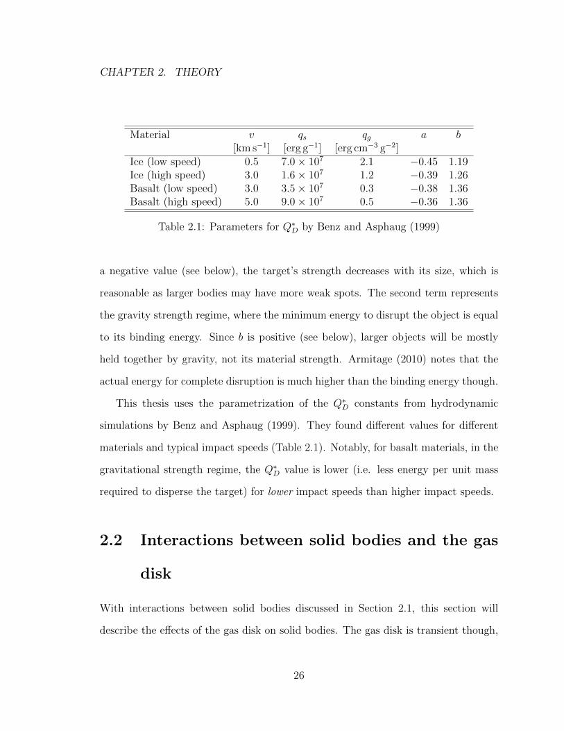
Material v qs qg a b[km s−1] [erg g−1] [erg cm−3 g−2]
Ice (low speed) 0.5 7.0× 10⁷ 2.1 −0.45 1.19Ice (high speed) 3.0 1.6× 10⁷ 1.2 −0.39 1.26Basalt (low speed) 3.0 3.5× 10⁷ 0.3 −0.38 1.36Basalt (high speed) 5.0 9.0× 10⁷ 0.5 −0.36 1.36
Table 2.1: Parameters for Q∗D by Benz and Asphaug (1999)
a negative value (see below), the target’s strength decreases with its size, which is
reasonable as larger bodies may have more weak spots. The second term represents
the gravity strength regime, where the minimum energy to disrupt the object is equal
to its binding energy. Since b is positive (see below), larger objects will be mostly
held together by gravity, not its material strength. Armitage (2010) notes that the
actual energy for complete disruption is much higher than the binding energy though.
This thesis uses the parametrization of the Q∗D constants from hydrodynamic
simulations by Benz and Asphaug (1999). They found different values for different
materials and typical impact speeds (Table 2.1). Notably, for basalt materials, in the
gravitational strength regime, the Q∗D value is lower (i.e. less energy per unit mass
required to disperse the target) for lower impact speeds than higher impact speeds.
2.2 Interactions between solid bodies and the gas
disk
With interactions between solid bodies discussed in Section 2.1, this section will
describe the effects of the gas disk on solid bodies. The gas disk is transient though,
26

CHAPTER 2. THEORY
so these effects will be diminished over time. Following Kominami and Ida (2002),
this thesis assumes the gas decay can be treated as a simple exponential decay:
ρgas(t) = ρgas,0 e−t/τgas , (2.23)
where ρgas,0 is the initial gas density (which would depend on location in the disk as
well) and τgas is the decay timescale (i.e. one e-folding time).
2.2.1 Aerodynamic drag
The strongest effect on solid bodies due to the gas disk is aerodynamic drag. This
is computed as an extra force acting on the solid bodies in addition to gravity. The
drag force, Fgd depends on the relative velocity between the solid bodies and the gas
particles, vrel = v − vgas, and many constants related to the characteristics of both
the gas disk and the solid body. Adachi et al. (1976) show that the gas drag force
per unit mass (i.e. acceleration) can be written as
agd =Fgd
m= −CDπr
2sρgas
2mvrelvrel = −3
8
CDrs
ρgasρs
vrelvrel , (2.24)
where CD is the drag coefficient governed by the size and shape of the particle and rs
and m are the radius and mass, respectively, of the solid body. The equality on the
right comes from replacing the mass with the density of the solid body, ρs times its
volume (assuming uniform density). The aerodynamic drag force can be split into two
regimes based on λgas, the mean free path of gas molecules in the gas disk (Armitage,
2010). When rs < λgas, the regime is known as Epstein drag, and CD contains terms
that depend on the thermal properties of the gas. For the rs & λgas regime, known as
Stokes drag, the shape of the solid body and the molecular viscosity of the gas are the
important parameters incorporated in the CD term. Note that CD is not necessarily
27

CHAPTER 2. THEORY
a constant, as it may depend on v as well. Further details on the CD term can be
found in Armitage (2010) and Adachi et al. (1976), for example. In this work, both
regimes are important as the gas density is much lower in the outer Solar System.
For both regimes, the inverse dependence on rs means that smaller bodies will feel a
bigger aerodynamic drag force.
2.2.2 Type I migration
As a massive solid body moves through the gas disk, it will create wakes (i.e. regions
of gas particle overdensity) both interior and exterior to its orbit. These wakes are
caused by Lindblad resonances, which occur when the orbital frequency of the gas
particles in the disk5, Ωgas(r), are an integer (i.e. positive or negative) multiple of the
difference between the orbital frequencies of the solid body, Ωs, and Ωgas(r). These
resonances are important because they allow exchange of angular momentum between
the gas disk and the solid body. The locations of the Lindblad resonance, rL for a
solid body in a circular orbit with semimajor axis as is (Armitage, 2010)
rL =
(1± 1
m
)2/3
as , (2.25)
where m is a positive integer and the minus sign correspond to inner Lindblad res-
onances (rL < as) while the plus sign corresponds to outer Lindblad resonances
(rL > as). Thus, there is a range of rL values that are closely spaced near as but will
also extend both outwards and inwards from the planet. The orbital speeds depend
on distance from the star, so the gas particles at the Lindblad resonances rL will orbit
at different speeds and it will create a spiral pattern with the solid body at the centre
5To be precise, a Lindblad resonance actually occurs when the frequency of the radial oscillations,κ(r), in the gas particles’ orbits matches a multiple of Ωs − Ωgas(r). However for a system with alarge central mass so that gas particles follow nearly Keplerian orbits, κ(r) = Ωgas(r).
28

CHAPTER 2. THEORY
(see Figure 2.4), which forms the wake (Armitage, 2010). These wakes will exert
torques on the solid body, where the outer wake’s torque is negative and would cause
a loss of angular momentum from the solid body to the gas disk, while the opposite
is true for the inner wake (Goldreich and Tremaine, 1980; Ward, 1986).
For typical gas disk parameters (e.g. density, temperatures, etc.), Ward (1997)
found that the outer wake is dominant, which causes a net inwards migration due
to the angular momentum loss. However, Kley and Crida (2008) demonstrated that
both the rate and direction of Type I migration depends on the equation of state of
the gas (i.e. whether the gas disk is modeled to be isothermal or fully radiative) and
on the ratio M/M∗. In particular, they showed that for protoplanets up to 40 M⊕,
the migration could go in either direction.
In addition to the radial migration, the eccentricity and inclination of the solid
body are quickly damped by the tidal wakes. This may also be referred to as random
velocity damping. Combining both radial migration and random velocity damping
effects, Papaloizou and Larwood (2000) writes acceleration on a particle with velocity
v due to the Type I mechanism as a sum of the radial , eccentricity, and inclination
damping and finds that
aTI = − v
ta− 2(v · r)r
r2te− 2(v · k)k
ti, (2.26)
where k is a unit vector in the vertical direction and ta, ti, and te are timescales
for damping of a, e, and i, respectively. In this definition, Papaloizou and Larwood
(2000) expected inward radial migration and defines ta to be positive when angular
momentum is lost.
Finally, it’s important to note that Type I effects happen when the solid body is
of sufficient mass to cause only small perturbations (i.e. the wakes) in the gas disk.
29

CHAPTER 2. THEORY
-1.5
-1
-0.5
0
0.5
1
1.5
-1.5 -1 -0.5 0 0.5 1 1.5
Y [
AU
]
X [AU]
Figure 2.4: This plot shows the spiral pattern caused by Lindblad resonances arounda planet (black dot on the x-axis) on a circular orbit at a = 1 AU. The dashed linesmark circular orbits with a corresponding to the locations of the inner (red) and outer(blue) Lindblad resonances (Equation 2.25 for m up to 60). Since particles orbit atdifferent speeds (Ω ∝ a−3/2), the coloured circles are placed where a resonant particlewould be after one orbit of the planet if it had started on the positive x-axis as well.
30

CHAPTER 2. THEORY
As the protoplanet grows more massive, they become strong enough to significantly
alter the local gas disk density. Namely, the protoplanet is found to open up a gap
in the gas disk by clearing most of the gas in an annulus around the protoplanet’s
orbit. When this happens, protoplanet prevents any gas flow across the gap and its
migration becomes locked to that of the gas disk itself (Ward, 1997). This type of
migration is called Type II. In contrast, a protoplanet under Type I migration moves
through the gas disk.
2.3 Other dynamical processes
Although the gravitational interactions between solid bodies described in Section 2.1
and the gas disk interactions of Section 2.2 dominate the dynamical evolution of
particles in the Solar nebula, this thesis does consider one other effect that does not
fit in either category.
2.3.1 Poynting-Robertson drag
The Poynting-Robertson drag effect is caused by radiation from the central star.
Small bodies, such as dust grains, absorb energy from the central star as they orbit.
Robertson (1937) carefully considers the effects of general relativity to show that
when this excess energy is radiated away by the dust grain, this results in a loss of
momentum and thus the dust grain feels an effective drag force. Robertson (1937)
computes the acceleration of a dust grain due to this drag force to be
aPR =AL∗
md c 4πr2. (2.27)
31

CHAPTER 2. THEORY
This acceleration acts in the direction opposite to v. In Equation 2.27, A is effective
cross section of the dust grain (facing the star), L∗ is the power output from the
central star, md is the mass of the dust grain, c is the speed of light, and r is the
distance from the star. Thus, AL∗/4πr2 is the power incident onto the dust grain.
However, it’s more informative to write both A and md in terms of the size of the dust
grain, rd, to see the size dependence of this effect. When assuming uniform density,
ρd for the grain, and a spherical shape, it is shown that, like aerodynamic drag, the
Poynting-Robertson acceleration is inversely proportional to the dust grain radius:
aPR =π r2d
4/3πr3d c
L∗4π r2
=3L∗
16π c r21
rd. (2.28)
2.4 Planet formation by core accretion
The previous sections detailed the physics of specific interactions between solid parti-
cles and gas disks relevant to the planet forming process. The main phases of planet
formation, from dust to gas giants are outlined in this section.
2.4.1 Forming planetesimals from dust grains
The first stage of planet formation, growing kilometre-sized planetesimals from sub-
micrometre-sized dust grains, is not completely understood. Initially, dust grains
could be spread over the entire protoplanetary disk surrounding the central star.
Armitage (2010) shows that for dust grains up to 1µm, Brownian motion alone is
sufficient for dust particles to encounter each other often enough for efficient growth.
For small particles, collisions can be assumed to be mostly adhesive, since Q∗D is
inversely proportional to size (see Equation 2.22 and the corresponding section on
32

CHAPTER 2. THEORY
collisions). The dust grains will also settle towards the mid-plane of the disk and
this motion will help keep the encounter rate between dust grains high enough for
growth to millimetre or even centimetre sized objects (Armitage, 2010). Growth from
two-body accretional collisions is known as coagulation.
However, growth to metre-sized objects and beyond is still unclear. Again, Ar-
mitage (2010) showed that with the right particle-to-gas densities, coagulation could
happen fast enough for metre-sized dust particles to grow to km-sized planetesimals.
But the main problem is whether or not collisions between metre sized objects would
actually result in adhesion rather than fragmentation.
Another possibility is the ”Goldreich-Ward” mechanism, proposed by Goldreich
and Ward (1973). The settling of dust to the midplane could cause a gravitational
instability and allow rapid growth to occur in this region. That is, the dust will first
settle onto the midplane, where random fluctuations in surface density could cause
clumps of particles to form, which then fall onto each other and form planetesimals.
The biggest problem with this mechanism is the presence of turbulence in the gas
disk. Turbulence could stir up the settling dust disk and prevent clumps of particles
from ever forming (Weidenschilling, 1980). Thus, the simple version of this mecha-
nism (which does not account for turbulence) would likely fail to form planetesimals,
but with a fuller understanding and treatment of turbulence, the Goldreich-Ward
mechanism may still be feasible. For example, Johansen and Klahr (2010) were able
to form planetesimals as large as ∼1000 km from gravitational instabilities in their
hydrodynamical simulations.
Unfortunately, while experiments have been done to try to recreate adhesive col-
lisions between centimetre-sized dust grains (Wurm et al., 2005), it is much more
33

CHAPTER 2. THEORY
difficult to recreate collisions of metre sized objects in the laboratory. Thus, there is
a still a gap in understanding the formation of solids from metre to kilometre sizes.
However, structures such as the Asteroid Belt and the Kuiper Belt provide observa-
tional evidence that planets were indeed formed from kilometre sized planetesimals.
2.4.2 Runaway growth phase
Assuming that kilometre sized planetesimals are somehow formed, the next phase is
known as runaway growth. Wetherill and Stewart (1989) first discussed this process
analytically and Kokubo and Ida (1996) showed that N-body numerical simulations
agreed with the analytical relationships. The original work came to this result using
kinetic gas theory to model the dynamical evolution of the swarm of planetesimals.
They argue that runaway growth is a consequence of equipartition of energy in ki-
netic theory, where the kinetic energy of the larger masses is equal to that of the
small masses so that larger bodies have smaller velocities. This is an outcome of
dynamical friction. Runaway growth often considers the case of several larger bodies
(planetesimals) of mass Mi in a swarm of many smaller planetesimals of masses m.
One of the larger masses, say M1, would be growing in this phase if the rate of change
of the mass ratio compared to the other large bodies is always positive, that is:
d
dt
(M1
M2
)> 0 . (2.29)
It can be shown that runaway growth will happen if (1/M)dM/dt is proportional
to Mβ with β ≥ 0. Physically, Kokubo and Ida (1996) show that the condition for
runaway growth happens when the velocity dispersion of the small bodies is larger
than that of the growing larger bodies (i.e. dynamical friction is effective), and
when the relative encounter velocities are less than the escape velocities (i.e. when
34

CHAPTER 2. THEORY
gravitational focussing is effective). These dynamical processes were discussed in the
previous sections.
Because a growing protoplanet can only accrete within its Hill sphere, the height
of the planetesimal disk is important. When the entire Hill sphere can be embedded
in the disk, the protoplanet can accrete in all 3 dimensions and Kokubo and Ida
(1996) show that this results in a growth rate of
1
M
dM
dt∝M1/3 . (2.30)
This will satisfy the condition for runaway growth (Equation 2.29). However, if the
disk is too thin (disk height is smaller than the planet’s Hill sphere), Kokubo and Ida
(1996) show that the growth rate is only
1
M
dM
dt∝M−1/3 , (2.31)
so runaway growth will not happen. Instead, the protoplanets exhibit orderly growth,
where all of the protoplanets grow slowly and roughly equally. This is related to the
next stage of planet formation.
Since the planetesimals start small, there will be some runaway growth until the
runaway condition is no longer met. If the disk is very thin, this could happen because
the runaway protoplanet’s Hill radius grows bigger than the disk and encounters are
no longer efficient enough to sustain runaway growth. In addition, runaway growth
is only possible if the protoplanet is not yet massive enough to dynamically excite
the planetesimals (i.e. increase their eccentricity), which would increase the rela-
tive encounter velocity and thus decrease the effectiveness of gravitational focussing.
Consequently, runaway growth will eventually stop as the protoplanet grows to a
large enough mass. The end result is a small fraction of the total planetesimals have
quickly grown to be much bigger than the remaining planetesimal disk and they are
35

CHAPTER 2. THEORY
still growing, albeit at a more even rate.
2.4.3 Oligarchic growth phase
The largest protoplanets in a given region cannot dominate the growth in the entire
planetesimal disk. Instead, there are many large protoplanets that are the fastest
growing body locally (in their region of the disk). Thus, these protoplanets are often
called oligarchs as growth is dominated by the oligarchs as a group. Because the con-
dition of stopping runaway growth are similar, these oligarchs will also tend to grow
to the same size and at the same rate. During this phase, the oligarchs scatter and
accrete planetesimals in their region. Kokubo and Ida (1998) argue that the scatter-
ing of planetesimal and dynamical friction combine to result in a net repulsion effect
between nearby oligarchs. These oligarchs end up separated by at least 5-10 mutual
Hill radii, where the mutual Hill radii is defined similar to rH in Equation 2.10 but
with the mass of the planet Mp replaced by the combined mass of the two oligarchs.
In addition, the oligarchs will accrete all of the planetesimals within their gravi-
tational reach and stop growing at what is known as their isolation mass, Miso. This
is mostly limited by the effective repulsion from other oligarchs. Assuming that their
orbits have also now circularized, a good estimate for the isolation mass is the sum
of all solid masses in an annulus extending 5 mutual Hill radii (if oligarchs are sep-
arated by 10 mutual Hill radii) in either direction (Kokubo and Ida, 2000). Thus,
Miso a function of the separation between oligarchs, ∆a, the orbital semi-major axis,
a, and the surface density of solids at the oligarch’s position, Σs(a) and corresponds
to the area of the annulus times the surface density: Miso = 2πa∆aΣs(a). But since
36

CHAPTER 2. THEORY
∆a ∝ rH ∝ aM1/3iso , this is an implicit equation where the relevant relation is
Miso ∝ Σ3/2s (a)a3 . (2.32)
The oligarchic phase ends when the oligarchs have reached their isolation masses.
In the terrestrial planet zone, (a . 2 AU), simulations show that the oligarchs reach
their isolation masses of 0.01− 0.1M⊕within 0.01− 1.0 Myr and are plentiful – their
numbers can range from 100 to 1000 oligarchs (Armitage, 2010). During this time
the oligarchs were on circular orbits, with low eccentricity and inclination due to
damping from aerodynamic drag and other gas disk effects (see Section 2.2). However,
as the gas disk decays, the oligarchs are able to become excited and their increased
eccentricities allow them to interact with one another and undergo collisions. Over a
long period of time, 10 − 100 Myr, these collisions eventually grow into the current
terrestrial planets (Armitage, 2010).
2.4.4 Atmosphere accretion on giant planetary cores
However, the gas giants followed a slightly different formation route. Unlike the
terrestrial planets, the protoplanets at the end of the oligarchic phase are not massive
enough to become gas giants. In particular, they do not contain much gas. Instead,
the protoplanets will end up forming the solid core of the gas giant, upon which the
gaseous atmosphere will be accreted from the solar nebula. As these cores grow, they
do accrete small amounts of gas and will have an envelope, which would help them
accrete planetesimals, or other cores, more efficiently (see Section 2.1.6). However,
in order to accrete the massive amounts of gas fast enough (i.e. before the Solar
nebula dissipates; see Section 2.2), Mizuno et al. (1978) and Mizuno (1980) show
that once the core reaches some critical mass, the envelope can no longer be in
37

CHAPTER 2. THEORY
hydrostatic equilibrium and will collapse onto the core. That is, the gravity of the
core overwhelms any pressure forces in the gas and causes an instability that results
in gas flowing rapidly onto the core and creating the gas giants of today. These
researchers also provide an estimate for the critical mass: about 10M⊕ is required.
However, considering that the gas disk is expected to dissipate within 10 Myr at
most (Kokubo and Ida, 2002; Levison et al., 2010), and that the terrestrial planets
took at least 10 Myr to grow about 1M⊕ in the inner Solar System (see Section 2.4.3),
then growing cores to the critical mass so quickly would be a problem. Furthermore,
Σs decreases at larger a, so collision (and thus growth) rates are slower in the outer
Solar System. Finally, Type I migration (see Section 2.2.2) effects may cause these
cores to be pushed in towards the star as they grow quickly in mass.
There are some factors that help giant planet core formation, though. Firstly, in
the Solar System, the gas giants exist beyond the snow line6 (also known as the ice
line), which is at around 2.7 AU (Armitage, 2010). Beyond the snow line, water and
other gas vapours freezes into icy solids and enhances the amount of mass available. In
addition, it may be possible that the cores begin formation closer to the star (where Σs
would be higher) and then migrated outwards to the present locations. The purpose
of this thesis is to use numerical techniques to explore how effective these factors,
as well as other effects such as fragmentation of planetesimals, can affect the giant
planet core formation.
6This is not always true in extrasolar systems containing so-called “Hot Jupiters”, for instance.
38

CHAPTER 2. THEORY
2.5 Planet formation by gravitational instability
In order to be complete, this chapter will close with a brief overview of an alternate
way to form planets. If core accretion is a “bottom-up” approach, then planet forma-
tion by gravitational instability would be a “top-down” method. This theory has gas
giant planets forming quickly out of gravitational instabilities in a thin gaseous disk.
That is, small over-densities in the gas disk result in local gravitational collapse, which
could then accrete more nearby gas particles and develop into planets. Thus, it could
be considered qualitatively like the Goldreich-Ward mechanism (see Section 2.4.1),
except with a gas disk instead of a planetesimal disk, and the end result is large gas
giants instead of large planetesimals. Numerical work by Boss (1997) show that this
model can indeed form gas giant planets for some types of gas disks and would do so
faster than core accretion models.
Armitage (2010) notes that there are also some issues with this model as well.
Namely, for the disk to become unstable enough to form gas giant planets, the disk
must be very massive and also must radiate away energy at a sufficient rate. These
constraints likely rule out the formation of Jupiter and Saturn in the Solar System
with this method. Gravitational instability may play a role in forming some gas giants
in extrasolar systems, but higher surface densities may also help core accretion models
as well. Armitage (2010) does conclude that the current observations of extrasolar
planets are consistent with the core accretion model but some of the most massive
extrasolar gas giants could form via gravitational instability.
39

Chapter 3
Previous Work
A crucial aspect of the core accretion model of giant planet growth is the critical
mass required for the solid protoplanet to cause rapid gas accretion from the gas
disk (see Section 2.4.4). Hence, the work by Mizuno (1980) could be considered the
beginnings of work on giant planetary growth by core accretion. Shortly afterwards,
another important idea, the Minimum Mass Solar Nebula (MMSN) was introduced
by Hayashi (1981). The MMSN is a solar nebula that contains all the solids necessary
to eventually form the planets and asteroids of the current Solar System, which is
about ∼0.01M or ∼3300M⊕ in gas and dust. The surface density of solids has a
power law profile, with Σs ∝ r−3/2, in the original MMSN model. Hayashi (1981)
also developed a model for the density of the gas disk and a combined gas and solids
surface density model, assuming solar composition, as well. Subsequent studies often
compare their initial conditions (e.g. the mass of the protoplanetary disks) to that of
the MMSN.
After the 1980s, although there has been many giant planet formation studies
40

CHAPTER 3. PREVIOUS WORK
in the past few decades, many of them are semi-analytical rather than a full N-
body treatment (e.g. Chambers, 2006, 2008), or a study of a single phase of giant
planet formation (e.g. Kokubo and Ida, 1996, 1998, 2000, 2002). This chapter will
discuss these studies and why they are not sufficient for completely modeling giant
planet core growth. Recently, (Levison, Thommes, and Duncan, 2010, hereafter
LTD10) did a full N-body simulation which is a systematic test of dynamical processes
mentioned in Chapter 2 and their effects on giant planetary core growth. This thesis
could be considered an expansion of LTD10, with less idealized initial conditions
and integration technique (see Chapter 4). Thus, the last section will describe the
simulations of LTD10 as it is the most relevant full numerical study of giant planet
formation and the result of this thesis will be compared to this previous work.
3.1 Semi-analytical work
The semi-analytical studies (e.g. Chambers, 2006, 2008) do include many of the ef-
fects discussed in Chapter 2 and found that it was possible to grow to the critical core
mass before the gas disk dissipates starting from protoplanets that are equal mass
(10−4M⊕) and evenly spaced at 10 mutual Hill radii apart. However, some dynamical
effects are not possible to model analytically: for example, a protoplanet could open
up a gap in the planetesimal disk, thus changing the disk’s surface density drastically
from an analytical expression. Another effect that has been observed in numerical
studies is so-called “planetesimal-driven migration” where a large amount of small
planetesimals, especially when massed together, can scatter off the protoplanets and
change its orbit. LTD10 did some test experiments to show that in the outer Solar
System, planetesimal-driven migration can be a stronger force than Type I migration
41
CHAPTER 3. PREVIOUS WORK
and could actually cause a protoplanet to migrate outwards. This happens because
the gas disk is denser in the region interior to the protoplanet’s orbit, particles that
are scattered inwards migrate inwards due to aerodynamic drag and be removed from
orbits that might encounter the protoplanet again. However, planetesimals scattered
outward will also migrate inwards due to aerodynamic drag so they will still encounter
the planets again. The inward scattering planetesimal increases the protoplanet’s an-
gular momentum but unlike the outward scattering planetesimals (which decrease
the protoplanet’s angular momentum), they don’t encounter the protoplanet again,
so this asymmetry could cause a net increase in the protoplanet’s angular momen-
tum, and thus cause outward migration (see e.g. Capobianco et al., 2011, for further
details).
3.2 Single formation phase work
The important and relevant results of studies looking at only one phase of giant planet
formation (including, but not limited to, Kokubo and Ida, 1996, 1998, 2000, 2002)
have been summarized in Chapter 2 in the subsections of Section 2.4 corresponding
to each formation phase. However, a recent and potentially interesting study by
Lambrechts and Johansen (2012) will be discussed here. They found that forming
giant planet cores from centimetre-sized objects (which they called “pebbles”) instead
of the usual kilometre-sized planetesimals may allow cores to grow at a rate that is
several orders of magnitudes faster, which would help get the cores to the critical
mass (see Section 2.4.4) before the gas disk dissipates.
Lambrechts and Johansen (2012) started their hydrodynamical numerical simula-
tions with an initial “seed” protoplanet of different sizes (equivalent to objects with
42

CHAPTER 3. PREVIOUS WORK
masses between 10−4M⊕ to 1M⊕ if their density was 1 g cm−3 and placed at 5 AU)
embedded in a 3 dimensional box of centimetre-sized pebbles with a surface density
equal to the MMSN. The scale height of the solids was set to be 0.01 times that the
gas scale height. Overall, the box of solids was chosen to ensure that the seeds were
embedded in a region of solids larger than the seed protoplanet’s Hill spheres. Then
they ran the simulations and computed the accretion rate for different initial seed
masses and planetesimal size, taking into account that they saw multiple stages of
accretion. By extrapolating these accretion rates, they computed the estimated time
to grow to the critical 10M⊕ value. Equation 44 of their paper show that it would
take just 40 000 years to form a 10M⊕ core at 5 AU in a MMSN when starting with
a seed planetesimal of ∼1000 km. Furthermore, their equation show that this time
scales linearly with distance from the Sun, so that it would take well under 1 Myr
even at distances out to 50− 100 AU. They compare it to work done by other studies
using metre and kilometre sized planetesimals and found that their rates are 102 and
104 times faster, respectively.
However, their work is not a full N-body simulation that would involve interactions
of the protoplanets with each other and the full planetesimal disk. So, despite being
a fully numerical computation, many of the processes (e.g. gap opening) that are
missing from semi-analytical studies are missing here as well. They also do not
allow their protoplanet to migrate, and assume a constant supply of pebbles as well
as a very large initial planetesimal. So, as in many of the studies mention above,
while Lambrechts and Johansen (2012) is able to show that a single phase of giant
core formation is possible, only a full N-body integration can piece all the phases
together (specifically, taking into account how the protoplanets might redistribute
43

CHAPTER 3. PREVIOUS WORK
the planetesimal disk) and to get the complete story.
3.3 Key processes in giant core formation (LTD10)
The preliminary simulations done in this thesis are heavily based on the work by
LTD10. In fact, the same integrator code was used for both works. Therefore, the
full description of the LTD10 integrator, which will be called the SyMBA-LTD10
integrator, will be saved for Section 4.1 as part of this thesis’ next chapter. But, for
this section, it is sufficient to note that LTD10 includes all of the effects as described
in Chapter 2 except for Type I migration (but eccentricity damping from the Type I
mechanism is included, see Section 2.2.2). Chapter 5 will further discuss the choices
in integrator parameters made by LTD10 and in this thesis.
3.3.1 Initial conditions
LTD10 used a 200M⊕ planetesimal disk spanning an annulus between 4 − 16 AU.
The gas and solids density profiles were set to be higher than the standard MMSN.
In fact, 200M⊕ of planetesimal mass in this region corresponds to a planetesimal disk
that is 6 times more massive than the MMSN. The planetesimals start on orbits with
low eccentricity and inclination. The gas and solids surface density profiles used by
LTD10 are similar to the profiles of the runs performed in this thesis, so the details
are in Section 5.1. The runs were integrated for 3 Myr of simulated time.
The protoplanets (called embryos by LTD10) were embedded in the planetesimal
disk between 4.5− 6.5 AU. There were five 1M⊕ embryos placed at separations of 10
mutual Hill radii. Their orbital eccentricity and inclination were set to be 10 times
44

CHAPTER 3. PREVIOUS WORK
smaller than the planetesimals’ average eccentricity and inclination.
Two key parameters are the radius of the planetesimals, Rp, and the radius of
fragments, Rf . Following the scheme described in Section 2.1.6, planetesimals that
collide can potentially fragment (in these simulations, they cannot accrete each other,
however). If they do fragment, then the resulting planetesimals are now called frag-
ments, with size Rf . For a given run, Rp and Rf each take only one value, so all
planetesimals will have the same size and all fragments will have the same size. From
run to run, LTD10 varied Rp between 1 − 100 km with a spacing of 0.5 dex1. When
fragmentation was turned on, the Rf values varied between 1 − 100 m, also with a
spacing of 0.5 dex. In addition to these parameters and toggling fragmentation LTD10
also looked at the effects of having embryo atmospheres, smaller embyo masses, and
evaporation and condensation of icy planetesimals at the snow line. Their goal was
to characterize how these dynamical processes affect core formation.
3.3.2 Fragmentation off
With fragmentation off and initial conditions as described above, the majority (90%)
of their runs showed little growth in embryos. With large planetesimals (Rp =
100 km), they report final embryo masses of 1.7 − 2.6M⊕. The end state show that
the embryos do not migrate very far from the starting points. In addition, the region
surrounding the embryos (4−7 AU) were almost completely cleared of planetesimals,
except for a few that are in a co-orbital resonance. However, of the 49M⊕ of planetes-
imals that started in this region, only 3.3M⊕ of mass was accreted by the embryos.
10.5 dex corresponds to a multiplicative factor of about 3.16, so Rp = 1 km, 3.16 km, 10 km ...
45

CHAPTER 3. PREVIOUS WORK
They report similar reports for other Rp values as well. This suggests that the em-
bryos could be very effective at changing the distribution of planetesimals, which
would affect growth rates. As mentioned before, semi-analytical studies would not be
able to consider this redistribution.
However, redistribution could also improve growth rates. LTD10 reports embryos
growing greater than 10M⊕ for some runs where the planetesimals are redistributed
into dense rings just outside of the embryo regions. If, by chance, the embryos’
interaction with one another ends up pushing an embryo into one of these rings, the
embryo can grow very rapidly. In the dense rings, the planetesimals are damped
by aerodynamic drag so that their eccentricities are low (“dynamically cold”), which
means their encounter velocities are low, which enhances accretion. This happens
more often for lower values of Rp since aerodynamic drag would be more efficient.
But this may be an unphysical effect because in their code, planetesimal-planetesimal
interactions do not result in excitation or accretion, so they are artificially forced to be
remain cold and dense (i.e. perfect targets for accretion). This issue will be addressed
in the improved code used in this thesis (see Section 4.2).
In the remaining 10% of runs without fragmentation, LTD10 saw the substantial
embryo growth through planetesimal driven migration. This process regularly created
embyros with more than 10M⊕; for example, at Rp = 10 km, they found an embryo
grew from 2M⊕ to 20M⊕ in about 100 000 years and migrated from 7 AU to 12 AU.
They also found that smaller Rp values lead to larger embryo masses and hypothesize
that smaller planetesimal sizes lead to more damping which makes accretion more
efficient. This is potentially a viable mechanism for core formation.
46

CHAPTER 3. PREVIOUS WORK
3.3.3 Fragmentation on
Keeping everything else the same, LTD10 turned fragmentation on by allowing plan-
etesimals potentially to collide, and for sufficiently energetic collisions, to fragment
from a particle with size Rp to one with size Rf . The idea was that having even
smaller particles around might further improve accretion efficiency. However, they
found that for Rf ≥ 30 m, the fragments end up being locked in mean motion res-
onances with the embryos. A mean motion resonance (MMR) happens when two
objects are in orbitals such that their orbital periods are integer ratios of one an-
other2. This causes the two objects to have repeated small gravitational interactions
with one another that could cumulate to a larger effect over time. In this case, the
“resonance lock” between the fragments and the embryos causes the fragments’ an-
gular momentum loss (due to inward migration from aerodynamic drag) to be shared
with the embryos, which causes them to migrate inwards as well. The total mass of
locked fragments can be large, in one example, LTD10 reports a total mass of 1.3M⊕.
On the other hand, for Rf ≤ 10 m, they found that the fragments were small
enough so that aerodynamic drag migrated them past potential resonance locking
orbits faster than they could be trapped. The smallest fragments also migrated past
the embryos before they could be accreted, though. They were only able to see
substantial embryo growth for a Rf = 10 m, where they see linear growth up to
38M⊕. Although these cores are very massive, the growth is only seen for a specific
values of Rf and aerodynamic drag parameters, so it may not be very robust.
2For example, Pluto is in a 2:3 MMR with Neptune, so that Pluto orbits the Sun twice in thesame time that Neptune makes 3 orbits. Objects in 1:1 MMR are on orbits with the same a but arenot in phase with each other.
47

CHAPTER 3. PREVIOUS WORK
3.3.4 Effects of embryo atmospheres
LTD10 found the effect of atmosphere enhanced accretion to be vital for embryo
growth. The runs with fragmentation (previous subsection) that showed the most
growth were repeated without atmosphere enhanced accretion. The largest embryos
only grew to 3M⊕ instead of all five embryos growing bigger than 10M⊕. They also
tried varying the opacity of the embryo atmospheres, (κ in Equation 2.20) by 5 orders
of magnitude but found only a small difference in final embryo mass (less massive at
higher κ because the collision cross section is smaller for larger κ). So while the
atmospheres are necessary, the embryo’s growth rate doesn’t depend on its opacity.
3.3.5 Effects of adding smaller embryos
One limitation of this code is that planetesimals are all one single size and one impor-
tant aspect for embryo growth (planetesimal driven migration) requires planetesimals
of a specific size. Ideally, if there was a large range of sizes for planetesimals, then
a group of planetesimal with the right size could exist. To slightly improve this
problem, LTD10 added 10 additional embryos to their initial conditions for runs
without fragmentation. These 10 embryos have a mass of 0.1M⊕ (∼Mars-mass) and
were distributed in the same region as the larger 1M⊕ embryos. Planetesimal driven
migration effects were much more common than before and the small embryos tend
to migrate out past their initial region and beyond the large embryos. In addition,
their interactions with the planetesimals in the outer disk causes planetesimals to be
scattered towards the inner disk where the large embryos can accrete them and also
migrate outwards and sometimes pushing the small embryos even further outward.
Overall, planetesimal driven migration was the norm when these small embryos were
48

CHAPTER 3. PREVIOUS WORK
added and regularly resulted in the large embryos growing to 10M⊕ or greater. How-
ever, when LTD10 tried introducing these small embryos to runs with fragmentation,
in hopes that the outwards migrating embryos would disrupt the resonance locked
fragments, they found that it was unsuccessful.
3.3.6 Beyond LTD10
The aim of this thesis is to improve on the investigations of LTD10 with less idealized
initial conditions and improved integration code to overcome some of their limitations.
The work in this thesis consists of two main groups of simulations. The first group are
some preliminary simulations using the same code as LTD10 but with improvements
to the initial conditions. Specifically, two important changes include a spectrum of
embryo sizes, and initial conditions generated so that there is a consistent relationship
between the initial embryo masses and the planetesimal disk.
The second group of simulations make up the main work of this thesis and uses
a different integrator (written by the same authors as LTD10) that addresses some
of the major issues in the SyMBA-LTD10 integrator. This code, named LIPAD
for a Lagrangian Integrator for Planetary Accretion and Dynamics (Levison et al.,
2012), will be described in Section 4.2. A major change from LTD10 is the ability to
represent a spectrum of planetesimals sizes by redefining tracer particles to simulate
planetesimal accretion and also allowing them to be promoted to an embryo.
The remaining chapters will describe the integrators and initial conditions used
to go beyond the work of LTD10 and presents results obtained thus far.
49

Chapter 4
Integrators
This methods chapter will discuss the integrators used in this thesis. In Section 4.1,
the idea of symplectic integrators and the symplectic massive body algorithm (SyMBA;
Duncan et al., 1998), which forms the core for all integrator code in this thesis, will
be discussed. The same section will also discuss the modifications to SyMBA in order
to end up with the integrator used for this work’s preliminary simulations: SyMBA-
LTD10. The modifications involve the addition of a new type of particle, fragments,
which could be created from planetesimal collisions. This addition allows simulations
to contain two different particle sizes in addition to embryos.
Next, Section 4.2 discusses a new code by Levison et al. (2012), LIPAD (La-
grangian Integrator for Planetary Accretion and Dynamics), which is based on the
SyMBA-LTD10 code. The major innovation of this code is the ability for planetes-
imals to take on a whole range of sizes. Planetesimal collisions can now result both
larger (through accretion) or smaller (through fragmentation) planetesimals. In ad-
dition, particles are able to be promoted or demoted from one class to another. That
is, while SyMBA-LTD10 and similar code require initial seed embryos to be manually
50

CHAPTER 4. INTEGRATORS
added, LIPAD allows embryos to grow naturally from an initial disk of planetesimals
that interact with one other and eventually grow. Thus, it is possible to run simula-
tions that cover several stages of planet formation. The creators of LIPAD have been
doing tests on terrestrial planet formation and this thesis represents a first attempt
of using LIPAD in the outer Solar System. It is also the first attempt of tackling the
giant planetary core formation problem with this type of integrator.
4.1 SyMBA-LTD10
4.1.1 Symplectic integration
Integrating particles in the N-body problem involves solving the equations of motion
discussed in Section 2.1.4. The Hamiltonian approach was used to get two first order
equations of motion (Hamilton’s equations, Equation 2.16), one for ri in terms of the
kinetic energy term, T , and one for pi, in terms of the potential energy term, V . To
simplify the notation, for now, this section will consider a single particle in a central
potential V so that the subscripts i here indicate time, not particle number.
A simple approach would be to use the T term to solve for ri, apply this velocity
for a single timestep, τ , and update the position of every particle (i.e. ri+1 = ri+riτ =
ri + piτ). At the same time, the V term can be used to compute pi in order to get
pi+1 = pi + piτ . This can be repeated every timestep and is known as the Euler
method. Note that both ri+1 and pi+1 are computed and updated at the same time.
In a single timestep, the energy error grows as τ 2 (i.e. δE ∝ τ 2) and the total energy
error is proportional to the total integration time (Burns and Gladman, 2010).
A symplectic integrator improves on the Euler Method by simply first computing
51
CHAPTER 4. INTEGRATORS
and updating the p term to get pi+1, then updating r with this new value, so that
ri+1 = ri + pi+1τ . This small change results in a first order symplectic integrator
makes a big difference in the final energy error, with orders of magnitude improve-
ment for the same amount of computational work (Burns and Gladman, 2010). A
further improvement is known as a leapfrog algorithm, where the r coordinate is only
advanced by half a timestep, and this new position is used to advance p by a full
time step. Then, the new p is used to advance r by the remaining half timestep. This
results in the integrator starting with a half timestep update for r (also known as a
“drift” step because the particle is advanced in an unchanging potential during this
step), then followed by alternating full timestep updates of p (also known as a “kick”
step, as the new potential and thus acceleration is computed to change the particle’s
velocity without changing its position) followed by a full timestep update of r, with
each quantity using the most up to date value of the other in order to update them-
selves (i.e. “leapfrogging”) and ends with the final half timestep in r. This leapfrog
method is used in SyMBA (and thus SyMBA-LTD10) as well as LIPAD. In terms of
Hamilton’s equations and following Burns and Gladman (2010), it can be written as:
ri+1/2 = ri + τ2∂H∂p
∣∣pi
= ri + τ2∂T∂p
∣∣pi,
pi+1 = pi − τ ∂H∂r∣∣ri+1/2
= pi − τ ∂V∂r∣∣ri+1/2
,
ri+1 = ri+1/2 + τ2∂H∂p
∣∣pi+1
= ri+1/2 + τ2∂T∂p
∣∣pi+1
.
(4.1)
The energy error in the leapfrog method oscillates around zero, with an amplitude
proportional to τ 2, which is much better than the Euler method. The integrators
in this thesis use an additional method to further simplify computations for N-body
interactions in a Kepler potential. That is, in order to take advantage of the fact that
the orbits of particles can be thought of as mostly following conic sections with small
52

CHAPTER 4. INTEGRATORS
perturbations due to interactions with the other bodies in the system, a Wisdom Hol-
man Map (WHM) could be used (Wisdom and Holman, 1991). With this method,
instead of splitting the Hamiltonian into kinetic and potential energy terms, it is in-
stead split into terms representing the Keplerian interactions (the particle with the
central body) and the terms representing the interactions with the other bodies. It
turns out that both of these Hamiltonians are exactly solvable, so a WHM symplectic
integrator could use the appropriate analog of the leapfrog method above (Equa-
tion 4.1) where the evolution of the system due to the Keplerian terms is the “drift”
step while the interaction terms represent a “kick” step to perturb the Keplerian orbit
(to another Keplerian orbit).
4.1.2 SyMBA
WHM integrators must use the same timestep throughout the entire integration. If
a variable timestep is used, the energy error will no longer oscillate around zero;
instead, the average energy error would systematically grow over time. However, it
is desirable to use smaller timesteps when the perturbation is large, such as a close
encounter of two objects. With large timesteps, WHM tends to fail when integrating
close encounters but it would not be efficient to always integrate with a small timestep.
SyMBA is a WHM-based integrator that allows for a changing timestep during close
encounters. To achieve this, Duncan et al. (1998) uses heliocentric (i.e. the origin
is the central body) coordinates to apply the Keplerian drift and the kick from the
interactions. However, this requires an additional “drift” term to the Hamiltonian to
account for the motion of central body in the barycentric frame.
To handle the close encounters, SyMBA places shells of varying radii, Rk, around
53

CHAPTER 4. INTEGRATORS
a planet to represent regions where a smaller timestep is required. As a particle
crosses from the k-th shell to the (k+1)-th shell, the timestep is divided by an integer:
τk/τk+1 = M . It is important to note that in order to get around the energy problems
of dividing timesteps in a WHM-based integrators, SyMBA is actually operating at
a timestep that is very much smaller than τ . The gravitational force is decomposed
into terms Fk such that when a particle is outside of shell Rn+1, then Fk = 0 for all
k > n. Therefore, all of the higher order (k > n) “kick” terms are zero and all of the
tiny timesteps collapse into a bigger one. When n = 0, then the timesteps all collapse
to become τ . Thus, SyMBA does not actually change the timestep (and thus does
not suffer a growing energy error) but this process of handling close encounters can
be more simply expressed as a division of the timestep τ .
SyMBA is originally implemented with M = 3 and while SyMBA-LTD10 uses
M = 3, the LIPAD runs in this thesis use M = 4. During testing of LIPAD, on
rare occasions, very close encounters in LIPAD showed that M = 3 could not re-
solve the interactions properly. SyMBA is also normally implemented so that each
successive shells have radii that decrease by a factor of Rk/Rk+1 = 2.08. From ex-
perimentation with accuracy and computational cost, Duncan et al. (1998) starts to
recursively “decrease” the timestep (Rk=1) if a particle comes within 3 mutual Hill
radii of another.
The leapfrog method is easy to adapt for the recursively subdivided timestep as
the Keplerian drift term can be recursively divided into M sets of drift and kick terms,
with timestep τk/M . This recursive subdivision of timestep could theoretically go on
forever, but is practically limited by the eventual collision of the particles. If two
particles were to collide then SyMBA merges the two particles and conserves total
54

CHAPTER 4. INTEGRATORS
mass and momentum.
This SyMBA code handles the N-body evolution of particles in SyMBA-LTD10
and LIPAD. The following subsections will discuss the classes of particles found in
SyMBA-LTD10 as well as any additional analytical routines to model other dynamical
effects such as collisional damping.
4.1.3 Particle classes and tracer particles
As mentioned in Chapter 2, it would not be practical to treat all particles in the
same way because there may be up to 1029 planetesimals in a system (LTD10) so
two concessions are made. Firstly, particles are divided into different classes that are
subject to different analytical forces; they interact with each other and themselves
in different ways to simplify computations and save time. In SyMBA-LTD10, the
classes are embryos, planetesimals, and fragments. Secondly, for very small particles,
instead of including every single object as an individual particle in the integration, a
group of objects on similar orbits is represented by a “tracer” particle (idea developed
by Levison and Morbidelli, 2007). Thus, any interactions between objects within a
tracer are not computed numerically.
In SyMBA-LTD10, embryos are represented by individual particles but planetesi-
mals and fragments are represented by tracer particles. Interactions between embryos
are computed directly via the symplectic integrator algorithm mentioned above. In
addition, interactions between embryos and planetesimals, and between embryos and
fragments, are also handled directly. The total mass of a tracer is the sum of the
mass of all its constituent objects, so if an embryo merges with a planetesimal or
fragment, it is considered to have merged with all of the objects in the same tracer.
55

CHAPTER 4. INTEGRATORS
Since the embryos have atmospheres, their capture radius is enhanced as discussed in
Section 2.1.6.
4.1.4 Modeling dynamical effects
This subsection discusses other dynamical effects included in the integrator that are
not covered by the symplectic routines. Thus, these are analytical computations that
are computed along with the symplectic evolution. Each effect will be discussed on
its own. Figure 4.1 shows a schematic outlining the direct and analytical effects on
particles classes in SyMBA-LTD10. A summary of effects acting on each particle
class is provided in Section 4.1.5.
Self-gravity
Although planetesimals do not interact with each other through N-body routines,
the gravitational effect between planetesimals is modeled through a one dimensional
“particle mesh”. The planetesimals and fragments are binned based on their semi-
major axis into annuli that are logarithmically spaced. The mass in each annuli is used
to estimate the gravitational force that each planetesimal or fragment tracer should
feel from all the tracers in a given annulus. The particle mesh method is described
more fully in LTD10. This significantly reduces the number of computations required
to account for gravity between planetesimals. In order to save time, this gravitational
effect is only computed once every NT1 timesteps, which is a user-supplied integer
parameter. The acceleration is assumed to be constant throughout NT1 timesteps
as the planetesimals and fragments generally will not migrate very far in a short
time. In addition, the planetesimal and fragments are re-binned every NT2 timesteps,
56

CHAPTER 4. INTEGRATORS
Aerodynamic Drag
Embryos
Collisional dampingSelf-gravity
Aerodynamic drag
Fragments
Tracers can fragment
Type I damping
Planetesimal tracers
Figure 4.1: A schematic showing all of the particle classes included in SyMBA-LTD10.The colours correspond to the Figures in Chapter 5 showing simulation results. Blacktext near or under each class label lists the analytical routines affecting that class.Section 4.1.4 describes these routines. N-body interactions are not shown. The onlyN-body interactions are those involving the embryo class particles (among themselvesas well as with the other classes). The blue arrow and text show the only reclassi-fication possible: from planetesimal tracer to fragment tracer due to the collisionaldamping routines.
57

CHAPTER 4. INTEGRATORS
which is another user supplied parameter. This assumes the mass distribution of the
planetesimals and fragments do not change very much over NT2 timesteps. The values
for these parameters are found in Section 5.1.
Collisional damping
Collisional damping is a term used to describe the overall effects of physical inter-
actions between particles (see Sections 2.1.2 and 2.1.6). Inelastic scattering between
particles will damp random velocities and thus damp eccentricities and inclinations
and some inelastic collisions could result in the merger of two particles. Collisions
that are energetic enough can cause particles to break up into smaller components. In
SyMBA-LTD10, the collisional damping routines could lead to either random velocity
damping or fragmentation, but growth is not possible. These routines are not neces-
sary for embryos since these effects arise naturally out of the gravitational interactions.
However, as interactions between particles represented by tracers are not computed
numerically, analytical collisional damping routines are used to model planetesimal-
planetesimal interactions. Fragments are not collisionally damped in SyMBA-LTD10
because the code neither allows for further fragmentation nor accretion. With their
much smaller size, it is likely that aerodynamic drag would damp their motions much
faster than inelastic collisions. In addition, collisional interactions between embryos
and planetesimals (or fragments) are also not included in SyMBA-LTD10.
Since planetesimals are not individual particles in SyMBA-LTD10, a probabilis-
tic approach is used to model collisions. Following Levison and Morbidelli (2007),
SyMBA-LTD10 bins the planetesimal tracers into 1000 logarithmically spaced rings
from 2 AU to 60 AU. The code computes the mass in each bin and keeps track of
58

CHAPTER 4. INTEGRATORS
the velocity and position of every tracer that passes through each bin (known as
interlopers). These values and lists are updated every NT2 timesteps.
At every NT1 timesteps, each tracer has a probability pcol of colliding with another
planetesimal1,
pcol = nAringvrel∆t , (4.2)
where n is the three dimensional number density of the solids (i.e. planetesimals),
assuming all the solids are a certain size (this is simple in SyMBA-LTD10 since
all planetesimals have the same size, Rp), Aring is the area of the ring, vrel is the
relative velocity between the target tracer and the mean velocity of the solids disk,
and ∆t = NT1τ since this is only computed every NT1 timesteps. In addition, to
avoid double counting collisions, particles may only collide with a smaller particle.
The impactor’s velocity, vimp, is chosen to be the velocity of the tracer that passed
closest to the current position of the target tracer (from the list of interlopers). Note
that while the other tracers are used to estimate vimp, the collision is not actually
happening between these two tracers, so the target tracer is the only one affected.
vimp and Q∗D (see Section 2.1.6 and Equation 2.22) determines the size of the largest
remnant (mlr) of collision relative to the total mass involved in the collisions (mtot).
Benz and Asphaug (1999) found that for icy particles, (for the region investigated by
this thesis, the particles are considered icy as they are beyond the snow line), this
ratio is
mlr
mtot
≈ −0.6
(v2imp2Q∗D
− 1
)+ 0.5 . (4.3)
1Technically, it would be an encounter between two planetesimals. However, all planetesimalsrepresented by a single tracer must be the same size, and to avoid creating new tracer particles,whatever happens to one planetesimal will happen to all others in the same tracer. Therefore, forthe purposes of applying pcol, it could be possible to consider a tracer as a single planetesimal thatis representative of all the other planetesimals in the same tracer.
59

CHAPTER 4. INTEGRATORS
This ratio is used to determine the probability pfrag of a collision resulting in frag-
mentation,
pfrag = 1− mlr
mtot
. (4.4)
This simplification is necessary since a tracer can only represent planetesimals or
fragments of a single size, not a mixture. For a collision of a given vimp and Q∗D, one
would expect a fraction 1−mlr/mtot to be in fragments (by definition) so averaging
over a large number of collisions, this is equivalent to a fragmentation probability of
1−mlr/mtot.
After every collision, collisional damping sets the velocity of the target tracer
particle to be the average of its original velocity and vimp. If fragmentation occurs,
then the planetesimal tracer is demoted to the fragment tracer class. Everything
remains exactly the same except for the size of the bodies (changed from Rp to Rf ).
The total mass of the tracer is unchanged so it is equivalent to the same tracer
representing a larger number of smaller fragments.
Aerodynamic drag
Aerodynamic drag is computed as per the description in Section 2.2.1. Since this drag
is very weak for large particles, only planetesimal and fragments feel aerodynamic
drag. The drag is computed with the planetesimal or fragment size as the drag radius
and applied on the tracer particle. The code correctly determines the drag regime as
all the gas and particle parameters are known. The gas parameters, such as density,
are computed from the initial conditions and related parameters (see Section 5.1)
while the particle data comes from the numerical computations. In order to save
60

CHAPTER 4. INTEGRATORS
time, the gas drag is only computed once every NT1 timesteps, which the same user-
supplied integer parameter mentioned above. Again, this acceleration is assumed to be
constant throughout NT1 timesteps as the migration of planetesimals and fragments
generally would be small during this time.
Type I damping
Interactions between embryos and the gas disk are modeled by the Type I mechanism
(see Section 2.2.2). These drag effects on the embryos are computed at the same time
as the computations of aerodynamic drag on planetesimals and fragments. So, the
NT1 parameter affects this calculation as well. For SyMBA-LTD10, the semi-major
axis damping is turned off. As discussed in Section 2.2.2, it is unclear whether Type
I migration would be outwards or inwards. In order to explore the effects of other
parameters and dynamical processes on planetary core formation, it is desirable to
turn off this unknown effect. However, experimenting with both inwards and outwards
Type I migration parameters could be a future study. This work included inclination
and eccentricity damping from the Type I mechanism using equal damping timescales
for both e and i.
4.1.5 Summary of SyMBA-LTD10 effects
During one timestep, many analytical and numerical calculations are done to model
the various dynamical processes. The order, frequency, and duration of each process
is summarized in Table 4.1. The table also notes which particle classes are affected
by each process. It is worth noting that the analytical computations only happen
every NT1 timesteps. In addition, the analytical computations (with the exception
61

CHAPTER 4. INTEGRATORS
Process (in order applied) Classes affected Frequency DurationAerodynamic Drag P, F every NT1 timesteps NT1τ/2Type I damping E every NT1 timesteps NT1τ/2Self-gravity P, F every NT1 timesteps NT1τ/2SyMBA E, P, F every timestep τSelf-gravity P, F every NT1 timesteps NT1τ/2Aerodynamic Drag P, F every NT1 timesteps NT1τ/2Type I damping E every NT1 timesteps NT1τ/2Collisional damping P every NT1 timesteps NT1τReclassify tracers P to F every NT1 timesteps NT1τRebin tracers P, F every NT2 timesteps —
Table 4.1: This table summarizes all the analytical and numerical (i.e. SyMBA)computations completed in SyMBA-LTD10. The first column lists the processes inthe order they are applied (see Section 4.1.4 for a detailed description). The secondcolumn shows the particle classes affected by each process with the abbreviations:(E)mbryo, (P)lanetesimal tracer, and (F)ragment tracer. The analytical processes donot occur every timestep and some of them have effects that are split (see details inSection 4.1.5. This is summarized in the third and fourth columns.
of collisional damping) are split into two parts: the effect is applied for 12NT1τ time
before and after the numerical symplectic integrator step (SyMBA). This happens
every NT1 timesteps, so that the total duration of the effect is NT1τ time over NT1
timesteps. The collisional damping and subsequent reclassification only happen after
the SyMBA step and the only reclassification possible is from planetesimal tracer to
fragment tracer. Finally, the binning of tracers for the self-gravity and collisional
damping happens at the end of every NT2 timesteps.
Out of all the processes discussed in Sections 2.1 through 2.3, SyMBA-LTD10 did
not consider the following: dynamical friction, collisions leading to growth, Type I
radial migration, and Poynting-Robertson drag. Other than Type I migration, these
effects are implemented in LIPAD.
62

CHAPTER 4. INTEGRATORS
4.2 LIPAD
LIPAD is a new code that also uses SyMBA to numerically integrate orbits of particles
and tracers. However, there are many differences in the classification of particles,
the treatment of planetesimal tracer particles, and analytical routines (particularly
the collisional damping routines) that allow LIPAD to overcome some limitations of
SyMBA-LTD10. This section describes the differences between LIPAD and SyMBA-
LTD10.
4.2.1 LIPAD particle classes
In LIPAD, the planetesimal tracer class is modified to allow for the planetesimals
to change size. The mass of a tracer, mtr, is kept constant while the number of
planetesimals represented by the tracer, Np, varies according to the planetesimal size,
Np =Mtr
43πR3
pρp, (4.5)
where ρp is the planetesimal mass density, which is also a constant. Thus, while
all planetesimals represented by the same tracer must have the same size, unlike
SyMBA-LTD10, this size is no longer fixed. Instead, as planetesimals fragment, Rp
can decrease as necessary. Since the planetesimal tracer can now represent objects
that are created from collisions in SyMBA-LTD10, the fragment tracer class is no
longer necessary. Due to computing resource limitations, there is a lower limit on the
size of planetesimals represented by a tracer, Rp,min. For this thesis’ implementation
of LIPAD, Rp,min was set to 0.5 km, which is a little bit higher than the LTD10 Rf
size (0.001 km− 0.1 km).
63

CHAPTER 4. INTEGRATORS
Although the ability to vary Rp allows for representation of particles in the kilo-
metre sized range, a new particle class must be introduced to represents the smaller
objects. In LIPAD, when a collision creates planetesimals with size less than Rp,min,
the planetesimal tracer is reclassified as a dust tracer. Dust tracers no longer frag-
ment and in this implementation of LIPAD, they do not have any interactions with
the planetesimal tracers. However, they do interact with other classes through N-
body interactions (i.e. they can be accreted or scattered). The dust particles will be
affected by aerodynamic drag as if they had size Rp,min and they will also experience
Poynting-Robertson (PR) drag (see Section 2.3.1) as if they had size Rdust, which is
a variable parameter typically in the micrometre range. PR drag causes dust tracers
to spiral towards the central star unless they get accreted by an embryo.
In LIPAD, low velocity collisions can also cause planetesimals to grow in size.
When the planetesimals size, Rp is large enough so that the tracer represents just a
single particle (Np = 1), the particle is promoted to a new particle class known as
a sub-embryo. This class allows for a planetesimal tracer to grow into an embryo.
Sub-embryos are necessary because a newly formed sub-embryo has the same mass
as a tracer so N-body interactions between a sub-embryo and a tracer can result
in unrealistically large scatterings. Thus, the sub-embryos have N-body interactions
(allowing them to scatter and collide) with each other as well as the full-embryos (see
next paragraph). They also scatter planetesimal tracers and dust tracers. However,
they are only affected by planetesimal tracers through analytical routines that model
various dynamical processes, described below. That is, a close encounter between a
sub-embryo and any tracer particle will not change the sub-embryo’s orbit.
64

CHAPTER 4. INTEGRATORS
Through accretion of each other, planetesimal tracers, and dust tracers, sub-
embryos can grow in mass until they reach a threshold and are promoted to full-
embryos. This implementation of LIPAD sets the threshold to be 100 times the mass
of the tracer. A full-embryo has N-body interactions with every other particle type.
The term embryos will be used to collectively refer to both full- and sub- embryos.
Finally, like SyMBA-LTD10, all embryos have their collision cross-section en-
hanced by their atmospheres (see Section 2.1.6). But, unlike SyMBA-LTD10, the
LIPAD N-body routines do not assume every collision between embryos result in a
merger. Section 4.2.3 describe how LIPAD handles collisional damping of both em-
bryo classes. The following sections describe the analytical routines adapted from
SyMBA-LTD10 followed by those that are added or modified in LIPAD. Figure 4.2
shows the dynamical processes affecting the LIPAD particle classes.
4.2.2 Dynamical effects from SyMBA-LTD10
For completeness and easy referencing, this subsection discusses routines imported
from SyMBA-LTD10 with only minor changes. Refer to Section 4.1.4 for the descrip-
tion of their implementation in SyMBA-LTD10.
Self-gravity
The self-gravity routines from SyMBA-LTD10 were used with only a change in the an-
nuli binning of tracer particles. Since LIPAD is much more computationally involved,
fewer logarithmically spaced bins were used (see Section 5.1 for these parameters and
a comparison with SyMBA-LTD10). Only the planetesimal tracers are included in
the particle mesh self-gravity routines.
65

CHAPTER 4. INTEGRATORS
Planetesimal tracersDynamical frictionViscous stirring Collisional dampingSelf-gravityAerodynamic drag
Reclassify if Rp < Rp,min
PR dragAerodynamic drag
Sub-embryos
Promote if Rp > Rp,max
Full-embryos
Type Idamping
Promote if M > Mpromo
Dynamical frictionPlanetary migration
Dust tracers
Figure 4.2: A schematic showing all of the particle classes included in LIPAD. Thecolours correspond to the Figures in Chapter 5 showing simulation results. Blacktext near or under each class label lists the analytical routines affecting that class.Sections 4.2.2 and 4.2.3 describe these routines. Blue arrows and surrounding textshow conditions for promotion or reclassification of particle classes. Within the plan-etesimal tracer class, the collisional damping routines are responsible for changingRp (and thus the number of planetesimals represented by a tracer). N-body inter-actions are not shown. They are computed for all interactions involving any one ofthe two embryo classes with one exception: N-body interactions between tracers andsub-embryos do not change the sub-embryo’s orbit.
66

CHAPTER 4. INTEGRATORS
Aerodynamic drag
The aerodynamic drag routines from SyMBA-LTD10 were used. The dust tracer
particle class experiences aerodynamic drag acceleration as if they had a size Rp,min,
which is an overestimate of the size leading to an underestimate of the drag accel-
eration (however, the Poynting-Robertson drag, see below, could be calibrated to
account for the difference). Note also that as the gas disk decays (Section 2.2), this
drag force becomes less effective.
Type I damping
In LIPAD, the same Type I damping effects for sub- and full- embryos are computed
the same way as SyMBA-LTD10’s effects on embryos. That is, radial migration
damping (affecting a) is not considered due to uncertainty in the direction. However,
random velocity damping (affecting e and i) is in effect.
4.2.3 New and modified dynamical effects in LIPAD
Collisional damping in LIPAD
Collisional damping in LIPAD is handled in a similar way to SyMBA-LTD10. For
instance, only the planetesimal tracer class is collisionally damped through an analyt-
ical routine, which computes the probability of a collision, pcol (Equation 4.2), using a
number density computed by binning planetesimals. In SyMBA-LTD10, the particles
were binned 1-dimensionally, based on their value for a (i.e. rings). Since all plan-
etesimals have the same size in SyMBA-LTD10, this was enough to find the number
density and thus pcol. However, in LIPAD, planetesimals may have varying sizes, so
all planetesimal tracers are logarithmically binned in 2-dimensions, both in rings of
67

CHAPTER 4. INTEGRATORS
different a and bins of different planetesimal size (Rp). Thus, in each ring, and for
each size bin, n = n(Rp) can be computed (the number density of planetesimals, not
tracers) and this allows computation of pcol for impactors of a given size. To get the
total pcol from all sizes, the code integrates over the Rp bins smaller than the target
tracer’s Rp (to avoid double counting). In addition, as in SyMBA-LTD10, the veloc-
ity and position of all tracers that pass through a given (a,Rp) bin (i.e. interlopers)
are recorded. If a collision is determined to have happened for a given planetesimal
tracer (i.e. the target), the velocity of the interloper that passed closest to the target’s
position is used to determine the impactor’s velocity, vimp. This velocity is used to
determine Q, the kinetic energy of the impactor, per unit mass of the collision.
As in SyMBA-LTD10, the mass of the largest remnant was computed. However,
LIPAD uses the the work of Morbidelli et al. (2009) to determine the outcomes of a
collision. Benz and Asphaug (1999) and Morbidelli et al. (2009) expect to find one
large object (the largest remnant, which could be larger than either colliding object)
and a continuous distribution of fragments. The mass of the largest remnant, mLR,
as computed by Morbidelli et al. (2009) is:
mLR =
[−1
2
(QQ∗
D− 1)
+ 12
]mtot : Q < Q∗D[
−0.35(
QQ∗
D− 1)
+ 12
]mtot : Q ≥ Q∗D
, (4.6)
where Q∗D is defined in Section 2.1.6 (see Equation 2.22) and mtot is the total mass
in the collision, as before. If mLR is a negative number, LIPAD considers the collision
to have completely destroyed the planetesimal tracer, so the particle is demoted to
a dust tracer particle. Otherwise, as in SyMBA-LTD10, the collision could result
in fragmentation with probability pfrag = 1 −mLR/mtot. If fragmentation does not
happen, then the planetesimals of the target tracer will have a new size corresponding
68

CHAPTER 4. INTEGRATORS
to a planetesimal mass of mLR. This allows the planetesimals to potentially grow in
size. If fragmentation happens, then LIPAD must determine what size the fragments
are. Note that unlike SyMBA-LTD10, neither of these outcomes result in a change of
particle class – it just determines the Rp of planetesimals represented by the tracer.
Morbidelli et al. (2009) determined that the fragments have a continuous size
distribution n(Rf ) following a double power-law with exponent qfrag terminating
with the largest fragment having mass mLF , where
mLF = 8× 10⁻³Q
Q∗Dexp
[−(
Q
4Q∗D
)2]mtot , (4.7)
and, where the power law exponent depends on the size of produced fragment Rf :
qfrag =
−2.5 : Rf < R∗f
−10 + 7(
QQ∗
D
)0.4exp
[−(
Q7Q∗
D
)]: Rf ≥ R∗f
. (4.8)
The power law is split at R∗f to ensure the total mass of fragments is finite. The
value of R∗f is chosen such that the total mass of fragments is equal to mtot. The Rp
of the target planetesimal tracer is chosen from the cumulative distribution function
of the fragment size distribution, Ffrag(X). That is, a uniform random number U
is generated between 0 and 1 and Rp is set to the value that solves Ffrag(Rp) = U .
Thus, over a large number of collisions and fragmentations, the resulting sizes of
planetesimals would recreate the power law size distribution predicted by Morbidelli
et al. (2009).
However, Levison et al. (2012) notes that there is a problem with this algorithm
for modeling collisions. Consider a tracer, “A”, that is larger than (for example) 3
nearby tracers, “B”, “C”, “D”, so collisional damping is causing the planetesimals of
tracer A to grow. With the current algorithm, since tracers do not change their total
mass, the planetesimals in tracer A will have larger and larger Rp while their number,
69

CHAPTER 4. INTEGRATORS
NA decreases. In addition, since no actual tracer-tracer interactions are computed,
the planetesimals of tracers “B”–“D” remain present. This allows “A” to continue
to grow without running out of mass to accrete. This is a problem because in this
situation, one would like to see the planetesimals in “A” grow in mass and remain
constant in number, instead of decreasing, while the number of planetesimals in “B”–
“D” should decrease and slow down the growth of planetesimals in “A” (as it runs out
of mass to accrete). In addition, as “A” grows, one would expect to see more particles
(and mass) in the larger size bin instead of less. To address this problem, LIPAD
tracks the mass that should have been added to “A” as it grows. Once this mass is
large enough (equal to mtr), mass is “transferred” to one of “B”–“D” by changing
the Rp of one of these smaller tracers to be similar to the Rp of “A”. This does not
actually change the mass of any tracer but now there is a correct amount of mass
and number of particles in the larger size bin and an appropriate decrease in mass
and number of particles in the smaller size bin. LIPAD also keeps track of which size
bin is providing the collisions that causes “A” to grow and the mass is transferred to
a tracer randomly chosen with probability based on how much mass its size bin has
contributed to tracer “A”.
Physical collisions involving embryos
The above covered planetesimal collisional damping. In LIPAD, physical collisions
involving embryos (i.e. embryo-embryo or tracer-embryo collisions) are a result of
N-body integration, not analytical computations. In SyMBA-LTD10, all physical
collisions result in accretion, but LIPAD allows for more options. However, LIPAD
assumes two objects could be created: a large remnant with mass mLR computed
70

CHAPTER 4. INTEGRATORS
using Equation 4.6 and a piece of ejecta with mass mej = mtot−mLR. The following
paragraphs describe the possible outcomes (note that only one outcome is chosen):
If mLR ≤ mtr, then the largest object has less mass than a tracer, which is inter-
preted as a powerful collision resulting in both objects being completely destroyed.
The two objects are replaced with planetesimal tracers that represent planetesimal
of mass mLR and mass mLF (Equation 4.7). This is the only outcome that results in
mass being removed from the simulation. Levison et al. (2012) notes that this case
is rare and did not happen in their tests of LIPAD. In this thesis, this outcome also
never happened.
Otherwise, if mej < mtr/2, then the ejecta mass is very small; not enough to be
represented by a tracer. The objects are considered to have merged and they are
replaced with an embryo of mass mtot.
Otherwise, if mLR ≤ mtot/2, then there is more mass in fragments (i.e.. mej >
mLR). But to avoid creating more tracers to account for these fragments, both objects
are replaced with embryos of mass mtot/2.
Otherwise, if mej > mtr then both the ejecta and largest remnant are larger than
tracers so the collision results in an embryo with mass mLR and another with mass
mej.
Finally, if none of the above conditions apply, then an almost-perfect accretion is
assumed. One embryo will have mass mtot − mtr while the other becomes a tracer
that represents planetesimals with mass mLF (Equation 4.7).
This treatment requires a lot of simplifications that are necessary due to the
limitations of the code. For example, no partial accretion is allowed for tracer-embryo
collisions because perfect accretion happens if the ejected mass is less than mtr/2 and
71

CHAPTER 4. INTEGRATORS
no accretion happens (final case) otherwise. The authors of LIPAD argue that while
these simplifications are not ideal, they are preferable to the overly simplistic perfect
accretion models.
Viscous stirring
Viscous stirring is applied to planetesimal tracers to account for close encounters (but
not collisions, as these are part of the collisional damping routines) with larger ob-
jects. Again, since tracers are not individual particles, these encounters are computed
statistically. A probability of a close encounter, pgrav is computed with the encounter
cross section σ where σ is the cross section of the target planetesimal’s Hill sphere2,
in a similar manner to pcol. The 2-dimensional binning of tracers and record of in-
terlopers allow LIPAD to determine the velocity of the interloping particle. LIPAD
then computes a flyby (see Section 2.1.2) with impact parameter randomly chosen
up to the Hill radius. The target tracer’s velocity is then adjusted to account for the
acceleration caused by the simulated close encounter. LIPAD applies this effect to
planetesimal tracers every NT1 timesteps.
Dynamical friction
As discussed in Section 2.1.5, dynamical friction is the net effect of gravitational
interactions between an object moving through a swarm of smaller objects. LIPAD
computes this extra drag force following Equation 2.17. Due to the use of tracers,
gravitational interactions between planetesimals are not directly computed so this
extra acceleration is applied in an analytical routine every NT1 timesteps. In addition,
2If the scale height of the planetesimal disk, h, is smaller than the Hill sphere, then the σ is theunion of the Hill sphere’s cross section and a slab of height 2h.
72

CHAPTER 4. INTEGRATORS
sub-embryos do not have direct interactions with tracers either (see Section 4.2.1),
so this acceleration is also applied analytically every timestep. Full-embryos do not
have analytical dynamical friction effects applied because these arise naturally out of
the N-body gravitational interactions.
Planetary migration
Planetesimal driven migration has been observed to be important to embryos in previ-
ous works (e.g. LTD10 as described in Chapter 3). Again, these effects are an outcome
of gravitational interactions between an embryo and the planetesimal tracers, so an
analytical treatment is required only for the sub-embryo particles. LIPAD determines
close encounters between sub-embryos and tracers by computing the probability pgrav
in the same way pgrav was determined for the viscous stirring routines on tracers. The
interlopers are randomly chosen from tracers within 7 Hill radii, using the same a, e,
and i as the tracer but also forcing the other orbital elements so that the interloper
is in the encounter plane. Then, a small 3-body symplectic integration involving the
central star, the sub-embryo and the interloper is performed, first backwards for 10
synodic periods3, then forwards for 20 synodic periods. This integration is done as
an aside to the main integration and does not actually move any particles around in
the main simulation. The change in energy of the sub-embryo’s orbit is recorded and
the total energy change due to all the encounters in one timestep is converted to an
extra acceleration to be applied to the subembryo at the next timestep.
3i.e. the time for the interloper to return to the same position, relative to the central star,measured by an observer on the sub-embryo
73

CHAPTER 4. INTEGRATORS
Poynting-Robertson (PR) drag
Finally, LIPAD applies PR drag (see Section 2.3.1) only on the dust tracers using
Equation 2.27 to apply an acceleration on dust tracers every timestep. The size of
dust particles, Rdust is a user supplied parameter that is inversely proportional to the
PR drag acceleration.
4.2.4 Summary of LIPAD effects
LIPAD uses many more analytical calculations than SyMBA-LTD10 to model the var-
ious dynamical processes more accurately. The increased number of particle classes
and enhanced behaviour of the planetesimal tracer class also demand additional rou-
tines. Table 4.2 shows these procesess in the same manner as Table 4.1 did for
SyMBA-LTD10. As before, some analytical routines are split within a timestep (see
Section 4.1.5. Note that the new subembryo routines are not split and they occur
before the SyMBA step. LIPAD allows for particles to be reclassified during the
collisional damping routines as well as during the SyMBA step (due to N-body en-
counters). Both embryo types can be reclassified as any other LIPAD particle type
due to collisions and mergers. Planetesimal tracers can either turn into subembryo
particles or dust tracers. In this implementation of LIPAD, dust tracers can only be
accreted by one of the embryo classes or eventually be removed from the simulation
due to impact with the Sun.
74

CHAPTER 4. INTEGRATORS
Process (in order applied) Classes affected Frequency DurationAerodynamic Drag P, D every NT1 timesteps NT1τ/2Type I damping E every NT1 timesteps NT1τ/2Self-gravity P every NT1 timesteps NT1τ/2Dynamical Friction (S) S every timestep τPlanetary Migration S every timestep τPoynting-Robertson Drag D every timestep τSyMBA* E, S, P, D every timestep τSelf-gravity P every NT1 timesteps NT1τ/2Aerodynamic Drag P, D every NT1 timesteps NT1τ/2Type I damping E every NT1 timesteps NT1τ/2Collisional damping* P every NT1 timesteps NT1τDynamical Friction (P) P every NT1 timesteps NT1τViscous Stirring P every NT1 timesteps NT1τRebin tracers P, D every NT2 timesteps —
Table 4.2: This table has the same format as Table 4.1. It summarizes all the analyti-cal and numerical (i.e. SyMBA) computations completed in LIPAD. The first columnlists the processes in the order they are applied (see Sections 4.2.2 and 4.2.3 for adetailed description). The second column shows the particle classes affected by eachprocess with the abbreviations: Full-(E)mbryo, (S)ub-embryo, (P)lanetesimal tracer,and (D)ust tracer. The analytical processes do not occur every timestep and some ofthem have effects that are split (see details in Section 4.1.5. This is summarized inthe third and fourth columns. Note that dynamical friction is computed and appliedto different classes at different times. The starred lines indicate steps where particlescan be reclassified. Sub-embryos can be promoted to embryos due to accretion andmergers during the SyMBA step. In addition, collisions of embryos during this stepcan demote them to sub-embryo or tracer classes. Also, planetesimal tracers can bereclassified to sub-embryo particles or dust tracers during collisional damping.
75

Chapter 5
Results and Discussion
This chapter presents the results of simulations performed for this thesis. The
SyMBA-LTD10 integrator was first used for some preliminary simulations. The goal
of these simulations was to attempt to investigate the scenarios of LTD10 with less
idealized initial conditions. The LIPAD simulations are the main results of this thesis
and represents the first use of LIPAD in the outer Solar System. These results will
examine the effectiveness of dynamical processes that could lead to giant planetary
core formation from a cold disk of planetesimals. This chapter will first present and
compare the initial conditions for both sets of simulations as well as the simulations
of LTD10.
5.1 Initial conditions
The initial conditions and parameters are split into categories and justification for
their chosen values are discussed. The parameters for LTD10 , the preliminary simu-
lations, and the main simulations are compared. The first two simulations used the
76
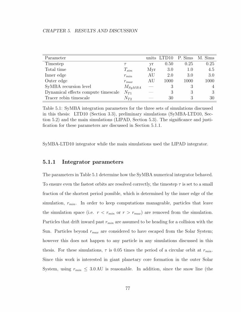
CHAPTER 5. RESULTS AND DISCUSSION
Parameter units LTD10 P. Sims M. SimsTimestep τ yr 0.50 0.25 0.25Total time Tsim Myr 3.0 1.0 4.5Inner edge rmin AU 2.0 3.0 3.0Outer edge rmax AU 1000 1000 1000SyMBA recursion level MSyMBA — 3 3 4Dynamical effects compute timescale NT1 — 3 3 3Tracer rebin timescale NT2 — 30 3 30
Table 5.1: SyMBA integration parameters for the three sets of simulations discussedin this thesis: LTD10 (Section 3.3), preliminary simulations (SyMBA-LTD10, Sec-tion 5.2) and the main simulations (LIPAD, Section 5.3). The significance and justi-fication for these parameters are discussed in Section 5.1.1.
SyMBA-LTD10 integrator while the main simulations used the LIPAD integrator.
5.1.1 Integrator parameters
The parameters in Table 5.1 determine how the SyMBA numerical integrator behaved.
To ensure even the fastest orbits are resolved correctly, the timestep τ is set to a small
fraction of the shortest period possible, which is determined by the inner edge of the
simulation, rmin. In order to keep computations manageable, particles that leave
the simulation space (i.e. r < rmin or r > rmax) are removed from the simulation.
Particles that drift inward past rmin are assumed to be heading for a collision with the
Sun. Particles beyond rmax are considered to have escaped from the Solar System;
however this does not happen to any particle in any simulations discussed in this
thesis. For these simulations, τ is 0.05 times the period of a circular orbit at rmin.
Since this work is interested in giant planetary core formation in the outer Solar
System, using rmin ≤ 3.0 AU is reasonable. In addition, since the snow line (the
77

CHAPTER 5. RESULTS AND DISCUSSION
distance from the Sun where water vapours condensate) is at ∼2.7 AU (Armitage,
2010), this ensures all solid bodies are icy.
The total integration time was Tsim = 3.0 Myr in LTD10 because that was their
estimated lower limit for the gas disk’s lifetime. However, LTD10 notes that most
of the characteristic features of each event was observed within the first 1 Myr, so
the preliminary runs only used Tsim = 1.0 Myr, which was sufficient to recreate the
results of LTD10 qualitatively. The main simulations used a longer Tsim to explore
both long and short gas disk lifetimes.
The SyMBA recursion level, MSyMBA was changed from default value of 3 to 4
for the main simulations (LIPAD) to ensure some rare close encounter events were
resolved correctly. The two timescales, NT1 and NT2 relate to the frequency that
certain analytical effects are applied and were further discussed in Section 4.2. These
parameters were chosen to increase computation speed without compromising accu-
racy. LIPAD is much more computationally expensive, which is reflected in some of
these parameters.
5.1.2 Gas disk parameters
Table 5.2 presents parameters of the gas disk and those related to dynamical in-
teractions between particles and the gas disk. All of these effects, most notably
aerodynamic drag, depend on the density of the gas disk, which takes the same form
as the one presented in Hayashi (1981):
ρgas(w, z, t) = ρgas,0
( w
1 AU
)−αgas
exp
[−z2
z2s(w)
]exp
[−tτgas
], (5.1)
where w and z are the cylindrical radius and height, respectively, and t is the time,
which is used to allow for gas disk decay. The ρgas,0 parameter is the mid-plane
78

CHAPTER 5. RESULTS AND DISCUSSION
Parameter units LTD10 P. Sims M. SimsGas diskGas density at 1 AU ρgas,0 g cm−3 3.4× 10⁻⁹ 3.4× 10⁻⁹ 3.4× 10⁻⁹
Gas power law exponent αgas — 2.25 2.25 2.25Scale height at 1 AU zgas,0 AU 0.05 0.05 0.05Gas disk inner edge agas,in AU 0.1 0.1 0.1Gas disk outer edge agas,out AU 1× 10³ 1× 10³ 1× 10³
Gas decay timescale τgas Myr 1× 1029 1× 1029
[1.55.0
]Type I MechanismRadial migration ca — 1× 10⁻²⁹ 1× 10⁻²⁹ 1× 10⁻²⁹
Eccentricity damping ce — 1.0 1.0 1.0Maximum mass MTI,max M⊕ 100 100 100Enhanced captureAtmosphere opacity κ κISM 0.02 0.02 0.02
Table 5.2: Gas disk parameters for the three sets of simulations discussed in thisthesis: LTD10 (Section 3.3), preliminary simulations (SyMBA-LTD10, Section 5.2)and the main simulations (LIPAD, Section 5.3). The square brackets indicate aparameter whose value varied between runs. The significance and justification forthese parameters are discussed in Section 5.1.2.
79

CHAPTER 5. RESULTS AND DISCUSSION
gas density at 1 AU and ρgas varies radially with a power law of exponent αgas. In
addition, its vertical profile decays as exp(−z2/z2s), and zs(w) is the scale height.
Adopting Hayashi (1981)’s temperature profile (where T ∝ w−1/2), the gas disk’s
scale height is
zs(w) = zgas,0
( w
1 AU
)5/4, (5.2)
where zgas,0 is the disk’s scale height at 1 AU. The parameters chosen in these simula-
tions represents a gas disk that is slightly shallower and more dense than the original
model of Hayashi (1981). Many gas effects also depend on the gas velocity, which
depends on w. The gas velocity, vgas is often related to the Kepler velocity (for a
circular orbit at a given distance from the Sun), vk through a parameter η, where
η ≡ 1
2
[1−
(vgasvk
)2]
= 6.0× 10⁻⁴(αgas + 0.5)( w
1 AU
)1/2. (5.3)
The gas effects are applied from agas,in to agas,out, which completely overlaps with the
simulation space. The gas disk decay timescale, τgas was set to a very large number
in LTD10 and the preliminary simulations which effectively turns off gas disk decay.
LTD10 cites studies showing the gas disk lifetime to be at least 3 Myr (with some
studies estimating it to be as high as 10 Myr) so they did not include τgas as a free
parameter and chose to explore other effects instead. However, as a result of LTD10
and the preliminary simulations, aerodynamic drag was found to be very effective at
indirectly causing embryo migration, so this effect was investigated by comparing the
effects of a short-lived versus long-lived gas disk.
Type I mechanism
The parameters ca and ce are used to determine the damping timescales for the Type
I mechanism, that is, ta and te in Equation 2.26. LTD10 argue that inclination
80

CHAPTER 5. RESULTS AND DISCUSSION
damping is less important than eccentricity damping, so ti was set to be equal to te.
The damping timescales also depend on the above gas disk parameters:
ta =1
ca
√a3
GM
(zs(w)
a
)2(Σgasπa
2
M
)−1(M
M
)−1(1 + ( ea1.3zs(w)
)5
1− ( ea1.1zs(w)
)4
), (5.4)
te =1
ce
√a3
GM
(zs(w)
a
)4(Σgasπa
2
M
)−1(M
M
)−1(1 +
1
4
(ea
zs(w)
)3), (5.5)
where local gas surface density is Σgas = π1/2ρgas(w, z, t)zs(w). As discussed pre-
viously, radial Type I damping was not included. ca was set such that ta would
effectively be infinite while ce = 1, following LTD10 and other similar works. Type
I damping is turned off for masses above MTI,max because very massive embryos will
redistribute the gas disk (open a gap). No embryos were observed to ever reach this
upper limit though.
Atmosphere enhanced collision cross section
To model the collision cross section enhancing effects of embryo atmosphere’s, one
additional parameter is required. κ is the opacity of the embryo’s atmosphere, in
terms of the interstellar medium’s (ISM) opacity. LTD10 found that the value of κ is
unimportant as long as κ > 0 and that a value of 0.02 is sufficient (see Section 3.3).
5.1.3 Parameters modeling other dynamical processes
Table 5.3 shows the number of radial and size (for LIPAD simulations only) bins for
planetesimal and fragment (in SyMBA-LTD10 only) tracers, which is used to compute
the dynamical processes not related to the gas disk (e.g. self-gravity). In LIPAD,
the minimum size bin is equal to Rp,min and the maximum size bin is equal to Rp,max
(see Section 5.1.4 and Table 5.4). Since LIPAD bins are 2-dimensional (size as well as
81
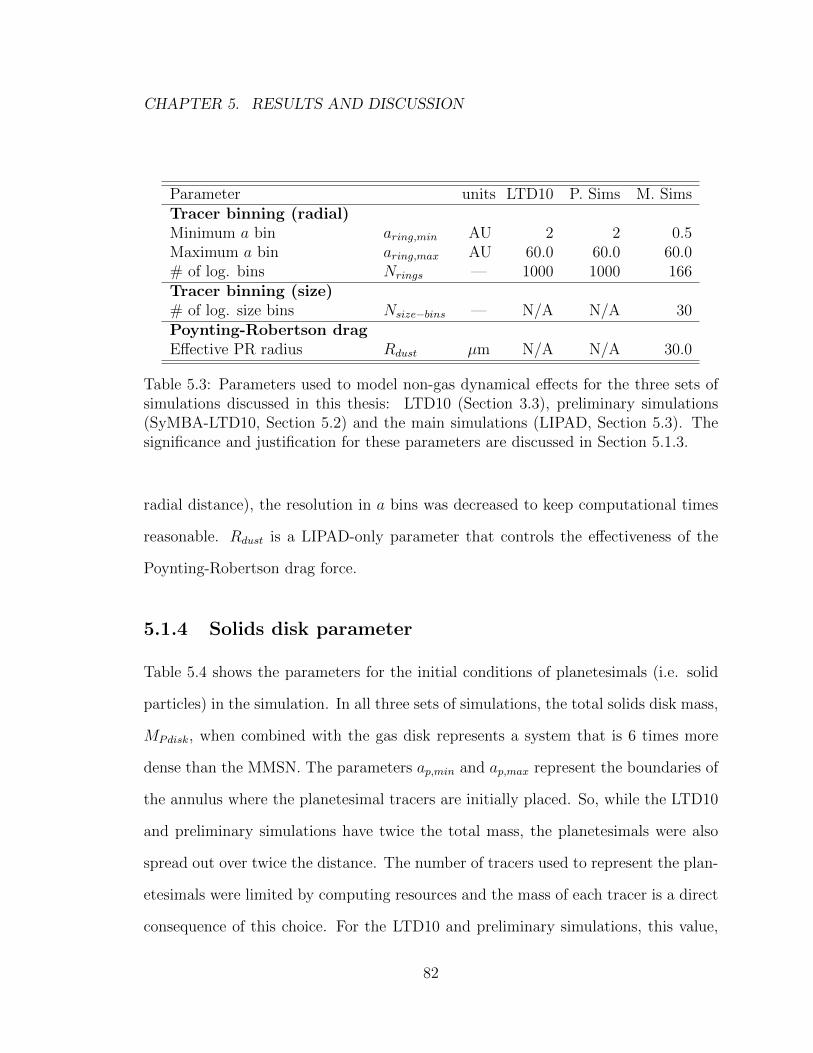
CHAPTER 5. RESULTS AND DISCUSSION
Parameter units LTD10 P. Sims M. SimsTracer binning (radial)Minimum a bin aring,min AU 2 2 0.5Maximum a bin aring,max AU 60.0 60.0 60.0# of log. bins Nrings — 1000 1000 166Tracer binning (size)# of log. size bins Nsize−bins — N/A N/A 30Poynting-Robertson dragEffective PR radius Rdust µm N/A N/A 30.0
Table 5.3: Parameters used to model non-gas dynamical effects for the three sets ofsimulations discussed in this thesis: LTD10 (Section 3.3), preliminary simulations(SyMBA-LTD10, Section 5.2) and the main simulations (LIPAD, Section 5.3). Thesignificance and justification for these parameters are discussed in Section 5.1.3.
radial distance), the resolution in a bins was decreased to keep computational times
reasonable. Rdust is a LIPAD-only parameter that controls the effectiveness of the
Poynting-Robertson drag force.
5.1.4 Solids disk parameter
Table 5.4 shows the parameters for the initial conditions of planetesimals (i.e. solid
particles) in the simulation. In all three sets of simulations, the total solids disk mass,
MPdisk, when combined with the gas disk represents a system that is 6 times more
dense than the MMSN. The parameters ap,min and ap,max represent the boundaries of
the annulus where the planetesimal tracers are initially placed. So, while the LTD10
and preliminary simulations have twice the total mass, the planetesimals were also
spread out over twice the distance. The number of tracers used to represent the plan-
etesimals were limited by computing resources and the mass of each tracer is a direct
consequence of this choice. For the LTD10 and preliminary simulations, this value,
82

CHAPTER 5. RESULTS AND DISCUSSION
Parameter units LTD10 P. Sims M. SimsPlanetesimal disk# of tracers Ntracers — 20 000 50 000 10 000Tracer mass mtr M⊕ 0.01 0.004 0.01Total disk mass MPdisk M⊕ 200 200 100Planetesimal bulk density ρp g cm−3 1.0 0.5 1.0Initial placementInner edge ap,min AU 4.0 4.0 4.0Outer edge ap,max AU 16.0 16.0 10.0Surface density at 1 AU Σs,0 g cm−2 16.7 16.7 16.7Σs power law exponent αsolid — 1.0 1.0 1.0Collisional evolution
Planetesimal size Rp km
1.003.1610.031.6100
1.00
10.0100
[5.0
30.0
]
Minimum Rp Rp,min km N/A N/A 0.5Maximum Rp Rp,max km N/A N/A 2 425
Fragment size Rf m
1.003.1610.031.6100
[
10.0100
]N/A
Full-embryo promotion Mpromo M⊕ N/A N/A 1.00
Table 5.4: Solids disk parameters and initial conditions for the three sets of simula-tions discussed in this thesis: LTD10 (Section 3.3), preliminary simulations (SyMBA-LTD10, Section 5.2) and the main simulations (LIPAD, Section 5.3). The squarebrackets indicate a parameter whose value varied between runs. The significance andjustification for these parameters are discussed in Section 5.1.4.
83

CHAPTER 5. RESULTS AND DISCUSSION
mtr is important because a large mass ratio between embryo and tracers is necessary
to have the embryos dominate the gravitational scattering of planetesimals. Thus,
with 2.5 times more particles, the preliminary simulations are a small improvement
over LTD10 in this aspect. However, in LIPAD, the additional of the sub-embryo
class and the analytical routines that go with the sub-embryos solves this issue. Also,
the minimum mass for promotion to full-embryo, Mpromo, sets a lower limit on the
full-embryo to tracer mass ratio, which is equal to 100 in the main simulations. Thus,
the number of tracers in LIPAD could be smaller, which is convenient as LIPAD is
more much computationally expensive.
The planetesimal bulk density, ρP , is the density of a single planetesimal in a
tracer, which determines the number of planetesimals represented by each tracer.
This should not be confused with the tracer’s spatial density, discussed next.
Initial placement
The planetesimal tracers were placed from ap,min to ap,max on orbits with a such that
the spatial density follows a power law:
Σs = Σs,0
( a
1 AU
)−αsolid
for ap,min < a < ap,max , (5.6)
where Σs,0 is the solids density at 1 AU. In the preliminary runs only, Σs is further
adjusted to compensate for the mass of the initial embryos. That is, at the locations
where the embryos are initially placed (see Section 5.1.5), the surface density here is
depleted by an amount consistent with the mass required to form the embryo. This
is another improvement in the initial conditions of LTD10. This is not an issue for
the main simulations since LIPAD starts with only planetesimal tracers.
84

CHAPTER 5. RESULTS AND DISCUSSION
LTD10 generated the initial e and i of the tracers by drawing from a Rayleigh distri-
bution with root-mean-squared (rms) values of erms = 0.01 and sin(i)rms = 0.005.
For the simulations performed in this thesis, initial conditions consistent with the
oligarchic phase of planet formation were used. In this stage, the planetesimal’s ec-
centricities are excited by interactions with the growing embryos and damped by
aerodynamic drag to reach an equilibrium value (Thommes et al., 2003)
etr,0 =1.7M
1/15P M
1/3em ρ
2/15P
b1/5C1/5D ρ
1/5gasM1/3a1/5
, (5.7)
where MP is the mass of a single planetesimal, Mem is the mass of an embryo that’s
exciting the planetesimal and b the spacing of the oligarchic embyros, in Hill radii.
For this approximation, CD was set to 1. In the preliminary simulations, Mem was the
closest embryo (out of the ones initially placed). In the main simulations, no initial
embryos were placed so the disk is very cold. To achieve this, Mem was replaced by
MP . The initial value was unimportant in LIPAD as the planetesimals quickly grew in
size and excited each other. Following LTD10 and Thommes et al. (2003), the initial
inclinations were set to etr,0/2. Thus, the planetesimal disk is very thin. All other
orbital elements (i.e. the angles) were randomly chosen from a uniform distribution.
Collisional evolution
Initially, all planetesimal tracers represent particles of the same size, Rp. Noting
that LTD10 had similar results at Rp ∼ 3 km as Rp ∼ 1 km, the spacing was much
coarser in the preliminary simulations. The main simulations only used two initial Rp
values due to time constraints. However, since LIPAD allows a tracer’s Rp to vary,
the initial values are not as important due to collisional damping quickly creating
smaller particles. In the SyMBA-LTD10 simulations only, the size for fragments is
85

CHAPTER 5. RESULTS AND DISCUSSION
also required. Again, the preliminary simulations had a coarser spacing than LTD10.
In addition, following LTD10, the preliminary simulations uses the Benz and Asphaug
(1999) parameters relating to high speed collisions between basalt (rocky) objects were
used to determine Q∗D (see Table 2.1).
In LIPAD only, it’s necessary to specify a minimum planetesimal size Rp,min due to
computational constraints. This was set to 0.5 km so the smallest initial Rp parameter
was 5.0 km instead of 1.0 km to allow for an order of magnitude between Rp and
Rp,min. The maximum size, Rp,max is the size such that the tracer only represents
one particle (i.e. promotion to sub-embryo). Promotion to full embryo is set to
100mtr = 1.0M⊕. These parameters are not used in the other simulations. Finally,
the LIPAD simulations used Benz and Asphaug (1999) parameters for low speed
collisions between icy objects to determine Q∗D instead as these parameters may model
particles in the outer Solar System more accurately.
5.1.5 Initial embryo placement
Table 5.5 shows the parameters used to determine the initial placement of embryos.
In LTD10, this was very straight forward. Five 1.0M⊕ embryos were placed between
4.5 AU and 6.5 AU, evenly spaced at about 10 rH apart. In some simulations, they
added ten 0.1M⊕ smaller embryos in the same a range. This results in a embryo to
tracer mass ratio of 100 for the big embryos but only 10 for the small embryos. The
embryo e and i values were about an order of magnitude smaller than those of the
planetesimals. In the main simulations, no initial embryos were placed.
However, as the preliminary simulations aimed to use oligarchic initial conditions
(as LTD10 used very idealized initial conditions), the embryo placement and masses
86

CHAPTER 5. RESULTS AND DISCUSSION
Parameter units LTD10 P. Sims M. SimsInner edge aem,min AU 4.5 4.5 N/AOuter edge aem,max AU 6.5 varies N/A
Embryo spacing b rH 10 10 10
# of embryos Nem —
[5
5 + 10
] [6
6 + 10
]N/A
Initial e eem,0 — 2× 10⁻³ 2× 10⁻⁶ N/AInitial i iem,0 rad 1× 10⁻³ 1× 10⁻⁶ N/A
Mass Mem M⊕
[1.0
1.0 + 0.1
] [2.0 . . . 0.2
2.0 . . . 0.2 + 0.1
]N/A
Bulk density ρem g cm−3 1.0 1.0 1.0
Table 5.5: The initial conditions for embryo placement in the three sets of simulationsdiscussed in this thesis: LTD10 (Section 3.3), preliminary simulations (SyMBA-LTD10, Section 5.2) and the main simulations (LIPAD, Section 5.3). The squarebrackets indicate a parameter whose value varied between runs. The significance andjustification for these parameters are discussed in Section 5.1.5. LIPAD does not haveany initial embryos but the b value is still used to compute the initial planetesimaleccentricities.
87

CHAPTER 5. RESULTS AND DISCUSSION
were more complex. There were three different sets of initial embryo placements used.
In all of them, there were 6 embryos spaced at b = 10 Hill radii apart. All embryos
had densities of 1.0 g cm−3. Their masses were computed using oligarchic growth rates
by Thommes et al. (2003), which depends on many factors such as the ρgas, ρP , and
so on. It is more useful to discuss the end result, which is a distribution of masses
approximated by the following power law
Mem,0(a) = M4.5
( a
4.5 AU
)−26/5, (5.8)
where M4.5 = 2.0M⊕ is the mass of the first embryo (at 4.5 AU). This value is
arbitrarily chosen. The other masses are 1.1M⊕, 0.7M⊕, 0.4M⊕, 0.3M⊕, and 0.2M⊕,
with the last embryo at 7.0 AU. Embryos less massive than 0.1M⊕ were omitted
since they interaction with the tracers would result in unphysically large gravitational
scatterings. The initial e and i were set to the same low value for all embryos. These
values are much lower than LTD10 because the tracers’ e and i were also much lower.
For the first set of simulations, these were the only embryos included. So, the embryo
to tracer mass ratio ranges from 500 to 50, which is an improvement over LTD10.
The other two sets of different embryo placements included 10 additional, smaller
embryos with mass 0.1M⊕. In the second set, the 10 smaller embryos were placed in
the same region as the large embryos, that is, starting at 4.5 AU and spaced b rH apart
(the last embryo was at 6.8 AU. In the third and last set, the power law (Equation 5.8)
was extended until an embryo with mass 0.1M⊕ was produced (8 embryos in total).
Then the remaining 8 embryos were forced to a mass of 0.1M⊕ and also spaced b rH
apart (the last embryo was at 11.2 AU). This effectively added a tail of smaller
embryos onto the original embryos. For these last two sets, the minimum embryo to
tracer mass ratio is only 25 but is still higher than LTD10.
88

CHAPTER 5. RESULTS AND DISCUSSION
5.2 Results of preliminary simulations (SyMBA-
LTD10)
The preliminary simulations were performed on the General Purpose Cluster super-
computer at the SciNet High Performance Computing Consortium (Loken et al.,
2010). The computations used Intel Xeon E5540 cores at 2.53 GHz and were paral-
lel (8 cores were used simultaneously). This section discusses the simulations using
3 different sets of initial embryo placement. Each set contained 9 simulations: 3
values of Rp with three fragmentation options (no fragmentation, Rf = 10 m, or
Rf = 100 m). Furthermore, 8 runs were performed for each simulation, for a total of
216 runs spanning 199 340 core-hours (22.7 core-years) of computational time. Only
a few representative runs will be discussed in this thesis. Simulation results are pre-
sented as snapshots of four different important time points and also as an animation
(MPEG format) as part of this thesis’ supplemental materials.
5.2.1 Set A: Large embryos only
The first set of preliminary simulations, called Set A here, started with only 6 embryos
from 2.0M⊕ to 0.2M⊕ from 4.5 AU to ∼7 AU.
In the case of no fragmentation, all the embryos survive to the end of the simula-
tion. Figure 5.1 shows an example run from this set where the largest embryo ends up
with a mass of 10.5M⊕. For Rp = 1 km, the embryos tended to accrete most of their
final mass within the first 0.15 Myr to 0.20 Myr (see Figure 5.2). They mostly grow to
masses between ∼5M⊕ to ∼10M⊕ and do not migrate very much from their original
positions, but there is a slight trend towards the Sun. However, two runs showed
89

CHAPTER 5. RESULTS AND DISCUSSION
the outermost embryo growing to ∼15M⊕ due to a sudden outward migration near
the beginning. In addition, the planetesimals that were not accreted were quickly
trapped in 1:1 MMR (i.e. co-orbital) with the embryos and gaps between embryos
rapidly form. This result shows slightly more growth than LTD10. The clearing of
planetesimals from the embryo’s region (other than those trapped in resonances) as
well as the lack of embryo migration are both behaviours also seen in LTD10 for the
same parameters.
At larger Rp values, the embryos tend to migrate outwards instead; the majority
of the embryos end up with 10 AU < a < 14 AU. This migration tends to excite
the entire planetesimal disk so that the planetesimals take awhile before they fall
into 1:1 resonances with the embryos. In addition, some embryos actually migrate
out as far as the outer edge of the planetesimal disk. Without additional material
further outwards, this migration is stopped and the embryos end up turning around
and migrating inwards again. At Rp = 10 km, the embryos grow quite large and the
mass of the largest embryo can be up to ∼60M⊕ (with a majority of them growing
larger than ∼30M⊕). This is the same effect seen in LTD10, namely planetesimal
driven migration. In the Rp = 10 km runs here, planetesimal driven migration was
the norm, but in LTD10, this only happened 10% of the time, unless the small 0.1M⊕
embryos were included. In this thesis, the embryos have a range of masses down to
0.2M⊕, so it is consistent that planetesimal driven migration is more common.
At Rp = 100 km, however, embryo growth is much smaller. The largest embryos
in each run range from ∼5M⊕ to ∼8M⊕, with a small number of cases reaching
∼12M⊕. Migration is still present though, and Figure 5.3 shows that unlike the
Rp = 1 km runs, the embryos will slowly accrete mass and migrate throughout the
90

CHAPTER 5. RESULTS AND DISCUSSION
Figure 5.1: Four snapshots (each snapshot consisting of a set of two panels) are plottedfor important time points (timestamp above the top panel). The panels plot particlemass (top) and eccentricity (bottom) against semi-major axis. In all preliminaryruns, embryo particles are plotted as blue circles, planetesimal tracer particles as redpoints and fragment tracer particles as black points. This figure represents a typicalrun from Set A with Rp = 1 km and fragmentation turned off. The embryos grow intheir original positions and migrate inwards slightly (Figure 5.2 shows the growth andmigration of the embryos over time). Planetesimals in the embryo region are eithercleared from it (most are gone by 0.3 Myr) or locked into 1:1 MMR with the embryos(a MMR exists at a specific a, so they appear as vertical stripes in the a vs. e panel).The outer planetesimals also migrate inwards due to aerodynamic drag but some aretrapped in higher order MMRs. By the end, only planetesimals locked in MMRs stillremain. This simulation is also available as an animation (MPEG format) as part ofthis thesis’ supplemental materials.
91

CHAPTER 5. RESULTS AND DISCUSSION
Figure 5.2: The mass (top panel) and semi-major axis (bottom panel) of all embryosare plotted against time for a run from Set A with Rp = 1 km and fragmentationturned off (the same run as Figure 5.1). The six initially large embryos are plottedwith blue lines while the ten smaller embryos (in Sets B and C) are plotted with redlines. This run shows typical behavior, where the majority of the accretion occursbefore 0.20 Myr. Some migration also happen before this time, followed by very slowbut steady inwards migration for the remainder of the simulation.
92

CHAPTER 5. RESULTS AND DISCUSSION
entire simulation. Bigger planetesimals result in more energetic collisions which mean
that fewer collisions result in accretion and bigger planetesimals are less affected by
gas drag, so that fewer outer planetesimals reach orbits that cross the embryos. This
could account for the decreased final masses in the Rp = 100 km runs compared to
the Rp = 10 km runs.
Therefore, the preliminary runs without fragmentation do show consistent results
with LTD10. With less idealistic initial conditions, specifically, the embryo initial
masses, planetesimal driven migration does appear more promising. However, there
appears to be a certain ideal range of planetesimal sizes (greater than ∼10 km but
less than 100 km) that are big enough to drive outward migration of planetesimals
yet are small enough to be efficiently accreted by the embryos. It is also promising
to see that the planetesimal driven migration is not just a result of the lower embryo
to tracer mass ratio used in LTD10.
When fragmentation is turned on for Set A, at Rf = 10 m, the embryos behave
in a similar manner as before for all values of Rp (that is, no embryo migration
for Rp = 1 km and outward migration for Rp ≥ 10 km). The planetesimals collide
with each other and generate fragments, which are much smaller and thus are more
strongly affected by gas drag. This causes the fragments to quickly flow past the
embryos, and they are small enough to result in rapid growth. The majority of the
fragments are created and migrate past the inner edge of the simulation space within
0.30 Myr. After this time, a small amount of fragments are still generated but the
prior collisions have excited the planetesimal disk to the point that collisions are no
longer frequent. Figure 5.4 shows embryo mass and semi-major axis plotted as a
function of time for a typical run with Rp = 1 km and Rf = 10 m and shows that the
93

CHAPTER 5. RESULTS AND DISCUSSION
Figure 5.3: Similar to Figure 5.2. This is a typical run from preliminary simulation setA with parameters Rp = 100 km and fragmentation turned off. Unlike the Rp = 1 kmrun, these embryos show steady growth and migration out to 10 AU to 14 AU overthe entire simulation. In addition, the innermost embryo (dashed line) experiencesthe most growth and become the only large embryo.
94

CHAPTER 5. RESULTS AND DISCUSSION
embryos reach their final mass by about 0.10 Myr. Their final masses are much larger
than cases without framgentation: at Rp = 1 km, 10 km, and 100 km, the largest
embryo in all runs is around ∼33M⊕, ∼33M⊕ and ∼18M⊕, respectively. This is also
consistent with LTD10, which found similar amount of growth for Rf ≤ 10 m and
rapid migration towards the Sun for Rf ≥ 30 m. The smaller fragments are migrating
fast enough to avoid resonance trapping and arrive in the embryo region and get
accreted. Figure 5.4 also shows that the innermost embryos are actually the one that
grows the most. This indicates that the fragments are moving too fast for the outer
(less massive) embryos to accrete them efficiently. This is supported by observations
of the low mass outer embryos migrating inwards (to become the innermost embryo)
early in some runs but the new low mass innermost embryo still does not accrete as
much as its more massive neighbours. So, while LTD10 saw the outermost embryo
growing the most (since they used equal mass embryos), a more realistic treatment
of embryo sizes suggest that for this fragment size, the larger embryos closer to the
Sun would grow faster.
However, when Rf = 100 m, the fragments end up trapped in resonances with
the embryos and the gas drag pushes the entire system towards the Sun. For Rp ≤
10 km, the last embryo is pushed past the inner edge of the simulation space within
0.15 Myr. Figure 5.5 shows the large groups of fragments moving inwards with the
set of embryos. This is also seen in LTD10. At Rp = 100 km, however, the embryos
migrate outwards early on. The outermost embryo ends up migrating outwards far
enough to not be trapped in the main group of fragments, so it survives while the other
embryos move towards the Sun. At this stage, it is able to accrete the planetesimal
and other newly formed fragments and grows to ∼13M⊕by the end of the simulation.
95

CHAPTER 5. RESULTS AND DISCUSSION
Figure 5.4: Similar to Figure 5.2. This run is a typical from preliminary simulationset A with parameters Rp = 1 km and fragmentation turned on (Rf = 10 m). Themajority of the growth and migration happens early in the simulation (≤ 0.1 Myr),similar to the result without fragmentation. However, with fragmentation, the em-bryos grow much larger. The inner 3 embryos (coloured solid lines) grow much largerthan the outer embryos (dashed lines).
96

CHAPTER 5. RESULTS AND DISCUSSION
In some cases, a large group of newly formed fragments exterior to the last embryo
end up causing the embryo to migrate inwards. However, in the majority of cases,
the last embryo ends up around at ∼12 AU by t = 1.0 Myr.
5.2.2 Set B: Large embryos with small embryos in between
Set B is a set of preliminary simulations where the ten additional 0.1M⊕ embryos
are added in the same region as the original six 1.0M⊕ embryos. As in LTD10 ,
these embryos were added to further enhance planetesimal-driven migration effects.
Since the small embryos are an order of magnitude less massive than some of the big
embryos, this could cause either small or large embryos to be scattered out past the
original embryo region, resulting in more growth.
Without fragmentation, the results with the added small embryos were very similar
to Set A. At Rp = 1 km, the planetesimals get trapped in 1:1 MMR and the embryos
clear planetesimals from their region, again. There is slightly more growth overall
and the final largest embryo masses are around ∼15M⊕ to ∼20M⊕. The initial small
embryos have about an equal chance of becoming the biggest embryo as the initial
large embryos. Figures 5.6 and 5.7 show a sample simulation where the largest embryo
reaches 17.4M⊕ and grew from one of the small embryos. Out of the original 6
embryos, the largest one grew to 12.4M⊕. In addition, although all the embryos
migrated outward slightly in the first 0.1 Myr, eventually all the embryos start moving
in towards the Sun. This does indicate that embryo migration is enhanced with the
addition of the 0.1M⊕ embryos.
At Rp = 10 km, the embryos migrate outwards a lot more and grow, and eventually
the planetesimals settle in 1:1 MMR with the embryos. This is the same behaviour as
97

CHAPTER 5. RESULTS AND DISCUSSION
Figure 5.5: Similar to Figure 5.1. This is a typical run from preliminary simulationset A with parameters Rp = 10 km and fragmentation turned on (Rf = 100 m). Thesnapshots show the embryos growing to ∼10M⊕ by 0.1 Myr. However, they are soonpushed towards the Sun by resonance trapped fragments (black). In the last frame,at only 0.28 Myr, all but one embryo has been removed from simulation space. Thissimulation is also available as an animation (MPEG format) as part of this thesis’supplemental materials.
98

CHAPTER 5. RESULTS AND DISCUSSION
Figure 5.6: Similar to Figure 5.1. This is a typical run from preliminary simulation setB with parametersRp = 1 km and fragmentation turned off. The inclusion of the smallembryos help them migrate outwards and grow for a very short time but then theyare pushed towards the Sun (see also Figure 5.7). Otherwise, the behaviour is similarto the Set A run with the same parameters, especially the clearing of planetesimalsand resonance trapping. This simulation is also available as an animation (MPEGformat) as part of this thesis’ supplemental materials.
99

CHAPTER 5. RESULTS AND DISCUSSION
Figure 5.7: Similar to Figure 5.2. This run is a typical run from preliminary simu-lation set B with parameters Rp = 1 km and fragmentation turned off (same run asFigure 5.6). These plots show that the added 0.1M⊕ embryos (red) end up migratingoutwards further than the large embryos (blue). In addition, the largest embryo wasoriginally one of the small ones.
100

CHAPTER 5. RESULTS AND DISCUSSION
Set A. The larger embryos appear to migrate outwards first and their migration may
be helped by scattering off the extra small embryos. Everything grows and the final
mass of the largest embryo is ∼33M⊕. Again, the largest embryo could come from
either the original six embryos or one of the additional 0.1M⊕ embryos. Although the
largest embryo in Set B at Rp = 10 km is smaller than Set A at Rp = 10 km, the total
masses of all the embryos is larger in Set B. Figure 5.8 shows the mass evolution of
a run from Set A and Set B with the exact same initial conditions other than the
additional 0.1M⊕ embryos.
At Rp = 100 km, Set B behaves shows the same result as Set A. The embryos
migrate outwards and grow slowly to produce one large embryo with a final mass of
6M⊕. However, it is only the original six large embryos that migrate out to ∼12 AU
and the largest embryo always comes from this set. Out of the initial 0.1M⊕ embryos,
the largest one tends to grow to only ∼1M⊕while many others embryos do not grow
at all. In addition, the initially smaller embryos do not migrate very much. At
Rp = 100 km, the gas drag is not very effective at moving planetesimals, so it makes
sense that the embryos which migrate would encounter more planetesimals and thus,
have more growth.
When fragmentation is turned on, the results are also very similar to that of
Set A. At Rf = 10 m, outward migration of the embryos is the norm, as in Set A.
The smaller embryos migrate out much further than the large embryos, especially at
Rp = 10 km. For this case, the initially large embryos only migrate out to the 6 AU to
8 AU range. As in Set A, the innermost (initially largest) embryos grow the most and
remain the largest at all Rp values. For Rp = 1 km, there are several large embryos
around ∼30M⊕ at the end. At Rp = 10 km, there are about 3 large embryos where
101

CHAPTER 5. RESULTS AND DISCUSSION
Figure 5.8: Similar to Figure 5.2. Two typical runs from Set A (left) and Set B(right) with Rp = 10 km and fragmentation turned off are compared. Other than theadditional 0.1M⊕ embryos (red) in Set B, the initial conditions are identical. Whilethe Set A run produces a single embryo that is larger than any embryo produced inthe Set B run, the latter run produces several embryos whose total mass is largerthan Set A’s total embryo mass.
102

CHAPTER 5. RESULTS AND DISCUSSION
the largest one is ∼35M⊕ and the next two are 2/3 and 1/3 of that mass, respectively.
At Rp = 100 km, there is only one large embryo at ∼20M⊕. These masses are all
consistent with Set A’s Rf = 10 m runs. At all Rp values, the smaller embryos do not
grow much at all: the largest ones usually reach ∼1M⊕while the remainder are only
a fraction of this mass, with many embryos not accreting anything at all.
When Rf = 100 m, the results are the same as Set A, again. For Rp = 1 km and
Rp = 10 km, the fragments are trapped in mean motion resonances with the embryos
and the entire system moves inwards towards the Sun. The only difference to Set A
is the timescale: it may take as long as 0.5 Myr for the embryos to be removed from
the simulation, which is about twice as long as the typical time seen in Set A. At
Rp = 100 km, the embryos tend to survive until the end of the simulation but by this
time, it is clear that they are on their way to the Sun. In one exceptional case out
of eight trials, shown in Figure 5.9, the entire set of large embryos actually expands
outwards slightly (to 9 AU) and then grows in place. Although the fragments do get
trapped in 1:1 resonances with the embryos, there is no massive cloud of fragments
forming exterior to the embryo system. Thus, the embryos survive without migration
and grow to produce 5 embryos between 12M⊕ and 17M⊕. The large embryos do not
migrate very much, but the small embryos do migrate outwards rapidly in the early
stages. This may have disrupted any potential fragment build-up in the outer Solar
System and prevented an inward migration of the embryos.
In summary, Set B adds small (0.1M⊕) embryos to the same region as the initial
oligarchic embryos to see what their effects may be on embryo growth and migration
rates. For runs without fragmentation, all of the embryos were observed to migrate
further which increases overall embryo growth. The Set B embryos may only grow
103

CHAPTER 5. RESULTS AND DISCUSSION
Figure 5.9: Similar to Figure 5.1. This is an exceptional run from preliminary simula-tion set B with parameters Rp = 100 km and fragmentation turned on (Rf = 100 m).Unlike all other runs with Rf = 100 m, the fragments do not get locked in a resonanceexterior to the massive embryos and cause inward migration of the entire system. In-stead, the larger embryos expand their region slightly and grow in place to form 5embryos with masses 12M⊕< Mem < 17M⊕. This simulation is also available as ananimation (MPEG format) as part of this thesis’ supplemental materials.
104
CHAPTER 5. RESULTS AND DISCUSSION
to ∼50% to ∼90% of the mass of Set A embryos; however, Set B produces a larger
number of embryos with a total mass that is greater than the total mass of Set
A embryos. For runs with fragmentation, the results are very similar to Set A,
especially showing one embryo that is much larger than the rest instead of several
nearly equal massed embryos. Set B includes one rare exception where the outward
migrating small embryos prevented a build-up of fragments in a resonance trap which
would have forced the embryos to migrate towards the Sun. The addition of small
embryos in Set B increased the rate of embryo migration due to two factors. Firstly,
planetesimal driven migration effects drive the 0.1M⊕ embryos more strongly than the
larger embryos. Secondly, the additional embryos are small enough to be scattered
by the original embryos. These interactions between embryos also cause all embryos
to have increased migration rates and ranges. This generally results in greater total
embryo growth in Set B runs.
5.2.3 Set C: Large embryos with small embyros added on as
a tail
Set C are preliminary simulations where the ten additional embryos are added as
an extension of the initial embryo region. This “tail” went as far as 11.2 AU. This
experiment was motivated by the observation that large rings of resonance trapped
particles, particularly fragments, that form exterior to the embryos tend to force the
entire system towards the Sun. Thus, the additional small embryos could prevent the
formation of these rings. In addition, they may also aid growth by scattering outer
planetesimals in towards the larger embryos or allow the larger embryos to migrate
outwards by scattering off the smaller embryos. With the oligarchic model of planet
105

CHAPTER 5. RESULTS AND DISCUSSION
formation, embryos would be expected to be present much further than the original
6.5 AU limit so this experiment is reasonable. However, a compromise is made in
using a minimum embryo mass of 0.1M⊕ in order to maintain at least a 25:1 embryo
to tracer mass ratio.
Without fragmentation, at Rp = 1 km, the embryos clear out their region except
for the planetesimal tracers trapped in 1:1 MMR with the embryo. This is the same
behaviour as Sets A and B. However, the tail embryos also migrate outwards early on.
This causes the entire system of embryos to actually migrate outwards for the entire
duration of the simulation. This is different from Set A (where everything migrated
inwards slowly) and Set B (where an initial outward migration turned into inward
migration). Figures 5.10 and 5.11 show a typical run with these characteristics. As
a result, the embryos reach large masses, even higher than Set B. The initially large
embryos tend to reach slightly higher masses (average largest mass ∼33M⊕) than the
tail embryos (average largest mass ∼21M⊕) and the largest mass tends to be about
50% to 75% larger than the next largest mass. There were two exceptions (out of
8 runs) to the outward migration, where a ring of resonance trapped planetesimals
formed exterior to all the embryos. It appears that when the tail embryos were
successful in disrupting the formation of resonance trapped planetesimal rings (most
of the time), planetesimal driven outward migration becomes the norm and results in
significant embryo growth. This type of initial embryo placement was not considered
in LTD10 but may lead to more opportunities for giant planetary core formation.
At Rp = 10 km, the results are similar to Sets A and B. The larger embryos
migrate outwards but the smaller tail embryos end up migrating inwards. In one
exceptional case (Figure 5.12), one of the small embryo migrates to the inner disk
106
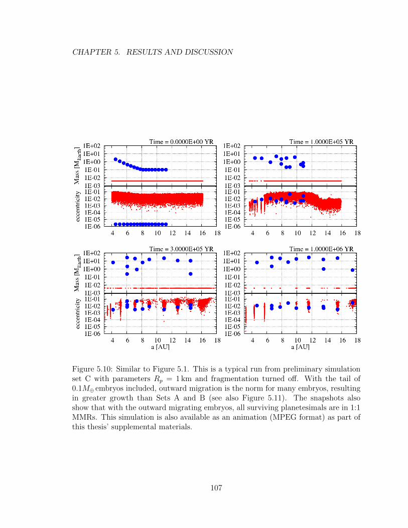
CHAPTER 5. RESULTS AND DISCUSSION
Figure 5.10: Similar to Figure 5.1. This is a typical run from preliminary simulationset C with parameters Rp = 1 km and fragmentation turned off. With the tail of0.1M⊕ embryos included, outward migration is the norm for many embryos, resultingin greater growth than Sets A and B (see also Figure 5.11). The snapshots alsoshow that with the outward migrating embryos, all surviving planetesimals are in 1:1MMRs. This simulation is also available as an animation (MPEG format) as part ofthis thesis’ supplemental materials.
107
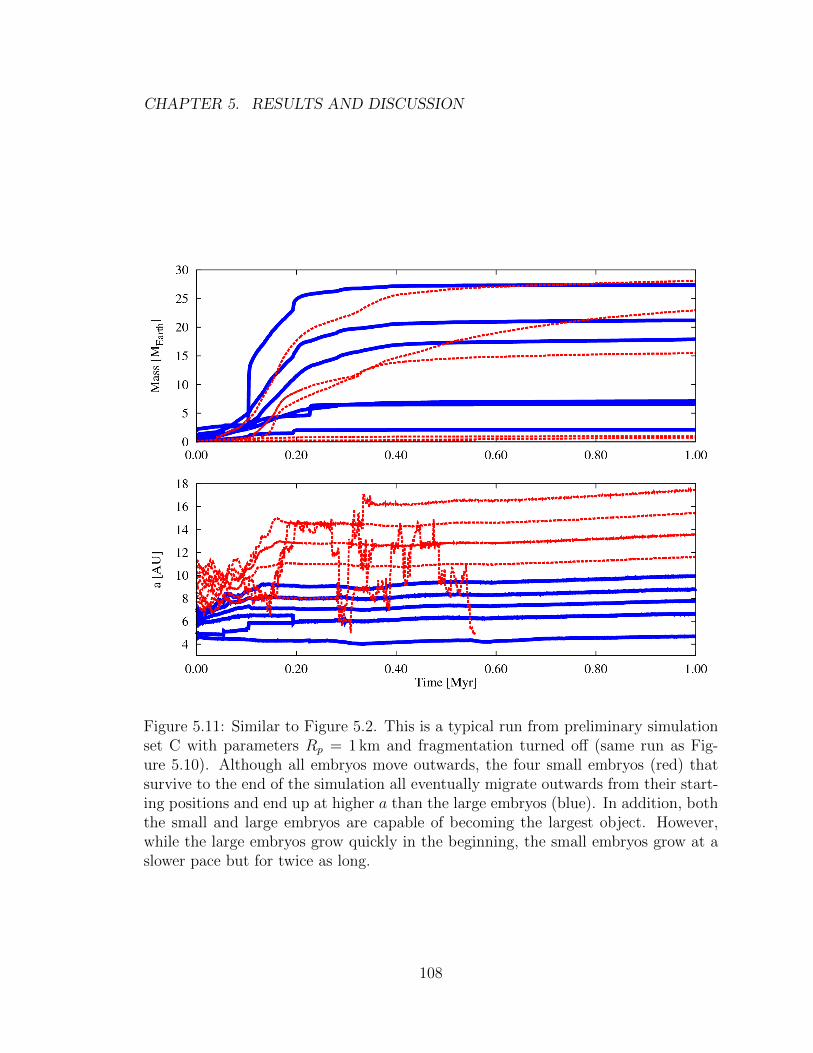
CHAPTER 5. RESULTS AND DISCUSSION
Figure 5.11: Similar to Figure 5.2. This is a typical run from preliminary simulationset C with parameters Rp = 1 km and fragmentation turned off (same run as Fig-ure 5.10). Although all embryos move outwards, the four small embryos (red) thatsurvive to the end of the simulation all eventually migrate outwards from their start-ing positions and end up at higher a than the large embryos (blue). In addition, boththe small and large embryos are capable of becoming the largest object. However,while the large embryos grow quickly in the beginning, the small embryos grow at aslower pace but for twice as long.
108

CHAPTER 5. RESULTS AND DISCUSSION
(∼4 AU) and quickly opens up a gap in the planetesimal disk (within 0.2 Myr), with a
ring of planetesimals trapped in a 1:1 MMR. This embryo enjoys substantial amounts
of growth as all inward flowing planetesimals are either accreted onto the embryo
or get trapped in the resonance. Near the end, another embryo gets trapped in
the same resonance and its interactions with the planetesimals there clear out the
resonance, leaving a wide (∼1.5 AU) gap surrounding a very large embryo with∼97M⊕
of material. In the other 7 runs, the largest embryos reach an average mass of about
∼30M⊕. Like Set B, each run results in a few embryos with these masses while the
remaining embryos end up at ∼5M⊕. In about half of the runs, one of the small tail
embryos end up being the largest embryo. Overall, the addition of tail embryos also
result in migration of embryos and growth and in one case, gap opening in the inner
disk is observed to dramatically increase accretion rates.
At Rp = 100 km, each run produces only one embryo with a mass of ∼6M⊕ and
another embryo with a mass of ∼2M⊕. The remaining embryos are under 1M⊕.
This is the same result as Sets A and B. The embryo migration is a little different
though. The larger embryos migrate outwards while the tail embryos migrate inwards,
resulting in embryos distributed between 5 AU to 15 AU. Although this placement
of embryos show that slow but steady outward migration does not happen when the
embryo disk is extended, the behaviour of the largest embryo appears to be the same
as before.
When fragmentation is turned on and Rf = 10 m, as in Sets A and B, the embryo
grows to larger masses than without fragmentation. As in Set B though, it is the
initial six large embryos that grow the most. The ∼0.1M⊕ tail embryos only grow
to ∼4M⊕ at Rp = 1 km and do not even get bigger than 1M⊕ for Rp ≥ 10 km. The
109
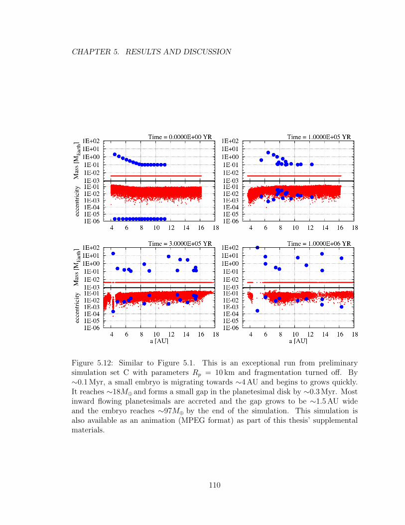
CHAPTER 5. RESULTS AND DISCUSSION
Figure 5.12: Similar to Figure 5.1. This is an exceptional run from preliminarysimulation set C with parameters Rp = 10 km and fragmentation turned off. By∼0.1 Myr, a small embryo is migrating towards ∼4 AU and begins to grows quickly.It reaches ∼18M⊕ and forms a small gap in the planetesimal disk by ∼0.3 Myr. Mostinward flowing planetesimals are accreted and the gap grows to be ∼1.5 AU wideand the embryo reaches ∼97M⊕ by the end of the simulation. This simulation isalso available as an animation (MPEG format) as part of this thesis’ supplementalmaterials.
110

CHAPTER 5. RESULTS AND DISCUSSION
innermost embryos show the most growth, and the largest embryo tend to reach
average masses of ∼32M⊕, ∼35M⊕, and ∼28M⊕ for Rp = 1 km, 10 km, and 100 km,
respectively. These numbers are similar to the results of Sets A and B. Figure 5.13
show a sample run with Rp = 100 km which has a large embryo growing to 26.6M⊕
while migrating outwards. The initial large embryos migrate outwards steadily and
grow at a roughly constant pace throughout the entire simulation (see Figure 5.13).
At Rp = 1 km, migration is not very strong (the large embryos migrate out to a
region between 5 AU and 10 AU. At larger Rp values, the innermost embryo migrates
between 2 AU and 4 AU (Figure 5.13 shows this for a typical Rp = 100 km run) and
results in the largest embryos spanning a region between ∼7 AU and ∼14 AU. In
these runs, the small tail embryos do not have a coherent migration pattern; their
encounters with the larger embryos tend to scatter them inwards while helping the
embryos migrate outwards.
When Rf = 100 m, the fragments are trapped in resonances that push the entire
system towards the Sun, as seen in Sets A and B. The tail embryos are usually not
enough to disrupt rings of resonance trapped fragments and prevent inward embryo
migration. However, the presence of these embryos does slow down the inward mi-
gration. It takes at least 0.5 Myr for the embryos to migrate past the inner edge
of simulation space. In several runs, many embryos still remain in the simulation
by 1.0 Myr but they are clearly migrating inwards towards the Sun. In a few cases,
one or more of the tail embryos might migrate past the outermost ring of resonance
trapped fragments and survive in the outer region of the planetesimal disk. However,
without much material to accrete at these distances, these embryos do not tend to
grow bigger than several Earth masses. These simulations show that expanding the
111
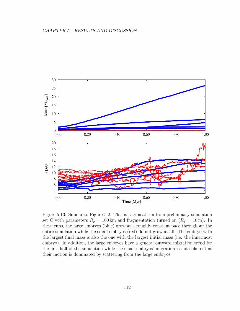
CHAPTER 5. RESULTS AND DISCUSSION
Figure 5.13: Similar to Figure 5.2. This is a typical run from preliminary simulationset C with parameters Rp = 100 km and fragmentation turned on (Rf = 10 m). Inthese runs, the large embryos (blue) grow at a roughly constant pace throughout theentire simulation while the small embryos (red) do not grow at all. The embryo withthe largest final mass is also the one with the largest initial mass (i.e. the innermostembryo). In addition, the large embryos have a general outward migration trend forthe first half of the simulation while the small embryos’ migration is not coherent astheir motion is dominated by scattering from the large embryos.
112

CHAPTER 5. RESULTS AND DISCUSSION
embryo region further out in the disk does not result in the tail embryos growing
large enough to disrupt resonance trapped fragments completely. But their presence
does appear to excite the fragments enough to slow down the larger embryo’s inner
migration. This may make a difference if the gas disk is allowed to decay. Under some
circumstances, the embryos may survive long enough to outlive the gas disk (and thus
the aerodynamic drag forces on the fragments pushing everything inwards).
Set C results show that adding additional small embryos as a tail or in the same
region as the large embryos (as in Set B) do not make a large difference in the
masses of planetary cores produced. Placement of small embryos as a tail appears
to affect embryo migration, however. The large embryos tends to migrate outwards
while scattering the small embryos inwards. The tail embryos can also cause inward
migration due to resonance trapped fragments to be slowed compared to Sets A and
B, but they do not grow large enough to completely prevent the trapping of fragments.
5.2.4 Summary of preliminary simulations results
Table 5.6 shows a summary of all the different simulation parameters and initial
embryo placement options. An Rf value of 10 m appears to be the option result-
ing in largest number of embryos above 10M⊕ while Rf = 100 m runs consistently
result in inwards embryo migration. Rp ≥ 10 km runs also seem to produce more
massive embryos. For these parameters, embryo placement options do not seem to
greatly influence the final masses but adding ∼0.1M⊕ embryos does slightly increase
the embryo masses and greatly increases outward migration. As discussed in previ-
ous chapters though, the SyMBA-LTD10 integrator has many limitations that are
partially resolved by the main simulations, which uses the LIPAD integrator instead.
113

CHAPTER 5. RESULTS AND DISCUSSION
Rp SetRf = 10 m Rf = 100 m No fragmentation
[km] ML [M⊕] a ML [M⊕] a ML [M⊕] a
1
A 33 (35) 0 21 (30) − 9.6 (15) 0
B (large embryos) 36 (51) 0 33 (54) − 17 (25) 0B (small embryos) 2.4 (4.1) s 28 (43) − 14 (20) +
C (large embryos) 32 (37) + 12 (18) − 32 (41) +C (small embryos) 3.4 (4.4) + 23 (29) − 21 (29) +
10
A 33 (37) + 26 (31) − 41 (62) +
B (large embryos) 36 (43) + 26 (35) − 33 (36) +B (small embryos) 2.0 (2.9) + 25 (31) − 31 (48) +
C (large embryos) 35 (39) + 24 (33) − 28 (49) +C (small embryos) 0.4 (1.0) s 24 (28) − 35 (97) −
100
A 19 (20) 0 14 (17) − 7.6 (13) +
B (large embryos) 23 (31) + 19 (26) − 6.2 (6.5) +B (small embryos) 1.2 (1.9) s 1.7 (7.7) − 1.1 (1.7) 0
C (large embryos) 28 (47) + 20 (27) − 6.3 (6.9) +C (small embryos) 0.4 (1.3) − 2.7 (8.5) s 0.7 (1.4) −
Table 5.6: Summary of preliminary simulation results. In Sets B and C, there weretwo groups of embryos: those with initially larger masses (> 0.2M⊕) and those withinitially smaller masses (≤ 0.2M⊕). In Set B, the small embryos start in the sameregion as the large embryos, but in Set C, the small embryos are exterior to thelarge embyos. ML shows both the average and maximum (in parentheses) mass ofthe largest surviving embryo in each run. a shows the overall direction of embryomigration: (+) outwards, (−) inwards, (0) no migration, or (s) for scattered. Smallembryos may not show coherent migration direction if their motion is dominated byscattering off the large embryos.
114

CHAPTER 5. RESULTS AND DISCUSSION
5.3 Results of main simulations (LIPAD)
The main simulations were performed on the same machines as the preliminary sim-
ulations. These integrations were also parallel and used 8 cores simultaneously. The
simulations all start with just a planetesimal disk; the user is not required to place any
initial embryos as they can be formed from planetesimal interactions. This section
discusses three sets of simulations that correspond to three different LIPAD fragmen-
tation behaviours. Each set contained 4 simulations: the planetesimals either had a
small (Rp,0 = 5 km) or large (Rp,0 = 30 km) initial size and the gas disk had either
a short (τgas = 1.5 Myr) or long (τgas = 5.0 Myr) decay time. There were between 5
and 8 runs performed for each simulation, for a total of 73 runs spanning ∼115 000
core-hours (∼13.1 core-years) of computational time. The choice of parameters to
explore was discussed in Section 5.1. Again, only a few representative runs will be
discussed in detail here. For these simulations, animations (MPEG format) are also
available as a part of this thesis’ supplemental materials.
5.3.1 Set X: No fragmentation
The first set of main simulations, Set X, are simulations with fragmentation turned
off. So, Rp,min is set to Rp,0 and Q∗D is infinitely large, so that every collision results
in accretion. Although these conditions are not realistic, this set provides a baseline
for evaluating the effects of fragmentation. 5 runs were performed for each set of Rp,0
and τgas values, except for Rp,0 = 30 km and τgas = 5.0 Myr, where 6 runs completed
within the available computing time.
For runs with Rp,0 = 5 km and τgas = 1.5 Myr, ∼3 embryos form in a region
between 4 AU to 6 AU in most runs while one run had 3 additional embryos and they
115

CHAPTER 5. RESULTS AND DISCUSSION
formed out to 8 AU as well. The first sub-embryo tends to form within ∼0.084 Myr
near the inner edge of the disk. Tracers at greater distances are promoted to sub-
embryos soon after, so a wave of sub-embryo promotion spreads outwards through
the planetesimal disk. This feature is common in all LIPAD runs performed in this
thesis. The first full embryo promotion tends to take place closer to ∼2 Myr. This
timescale does vary a bit between runs, showing values as low as 1.34 Myr or as high as
3.49 Myr. The embryos end up with roughly equal masses, between 1.0M⊕and 1.8M⊕,
although one exceptional embryo reaches 2.8M⊕ by 4.5 Myr. The largest embryo in
each run has an average mass of 1.79M⊕. In addition, on average, 84 tracers are
promoted to sub-embryo status but only 30% embryos survive to the end (the others
are removed from the simulation by migration inwards past 3 AU or merging with
another embryo). About 1000 merger events are recorded per run, which is a useful
proxy for measurement of total accretion in a run. This number includes both mergers
between a tracer and an embryo (which is an accretion of mtr = 0.01M⊕) as well as
mergers between embryos (where no new mass is accreted). Since the former events
outnumber the latter, 1000 merger events approximately represents 10M⊕ worth of
accretion, although this number is a slight overestimate.
Increasing the τgas to 5.0 Myr results in both a greater number of embryos and
higher masses. The runs end up with about 5 embryos evenly spaced in a region
roughly between 5 AU and 10 AU in most runs. The embryos form a bit faster: the
first sub-embryo appears at ∼0.077 Myr and the first full embryo at ∼1.45 Myr. The
sub-embryos appear the same way as before. Typically, a couple of full embryos are
promoted first near the 4 AU region and they migrate outwards to their final positions
beyond 5 AU. Each run produces several embryos with masses between 2M⊕and 4M⊕
116
CHAPTER 5. RESULTS AND DISCUSSION
and the average mass of the largest embryo of each run is ∼3.9M⊕. However, fewer
embryos are promoted (74) while approximately the same fraction survive as before
(∼30%). There is a great increase in the number of mergers: ∼1600 events per run are
recorded, on average. The long gas disk lifetime appears to help accretion and growth
of embryos in this case. The gas drag force helps bring outer planetesimals into range
of the embryos but perhaps more importantly, damps the velocities of planetesimals
so that collisions resulting in growth happens more often. This results in embryos
forming faster and at higher masses. Figure 5.14 shows a run from this parameter set
where the embryos form near the inner planetesimal disk but then migrates outwards
by a significant amount. The four embryos end up with masses of 4.3M⊕, 2.3M⊕,
1.2M⊕, and 1.2M⊕. In addition, this run shows the first embryo starting to clear a
gap in the planetesimal disk.
At Rp,0 = 30 km and τgas = 1.5 km, the increased planetesimal size does not affect
the time for the first sub-embryo promotion very much (0.088 Myr) but the first full
embryo promotion is delayed compared to Rp,0 = 5 km. The average time is 3.1 Myr,
not including the one run that did not form any full embryos. Up to three embryos are
formed in each run with masses around ∼1M⊕. On average, 77 tracers are promoted
per run and ∼40% of embryos survive until the end. An average of 728 merger events
are recorded. Overall, these numbers show a decrease in both number and masses
of embryos. As in previous runs, this is a consequence of the increased difficulty of
accreting larger planetesimals since their eccentricities are less damped by gas drag
than those of smaller planetesimals. When the τgas is increased to 5.0 km, the numbers
follow the same trend as increasing τgas for the Rp,0 = 5 km runs. The time for first
sub-embryo and full-embryo promotion drops to 0.069 Myr and 2.21 Myr, respectively.
117

CHAPTER 5. RESULTS AND DISCUSSION
Figure 5.14: Four snapshots (each snapshot is a set of two panels) are plotted forimportant time points. The top panel plot the radius of an individual particle againstsemi-major axis. For tracers, this is Rp: the radius of a single dust or planetesimalrepresented by that tracer. On the secondary y-axis, the equivalent mass in M⊕ isshown. Again, for tracers, this is the mass of an individual planetesimal or dustparticle, not mtr (which is a constant). The bottom panel plots e against a. Inall main runs, full-embryos are plotted as large blue circles, sub-embryos as smallerblack circles, and both dust and planetesimal tracers appear as red points. Thedust particles have Rp = Rp,min so in Sets Y and Z, they are the red points withthe smallest radius. This run from preliminary simulation Set X with parametersRp,0 = 5 km and τgas = 5.0 Myr shows typical behaviour for LIPAD runs. Sub-embryos form throughout the whole planetesimal disk while full-embryos are firstpromoted near 4 AU. These embryos tend to migrate outwards and grow further,reaching masses of ∼2M⊕. In this run, the innermost full embryo starts to cleara gap in the planetesimal disk. This simulation is also available as an animation(MPEG format) as part of this thesis’ supplemental materials.
118

CHAPTER 5. RESULTS AND DISCUSSION
In addition, more full embryos are formed; each run results in at least ∼2 embryos
with masses between ∼1.2M⊕ and ∼3.0M⊕ and an average largest embryo mass of
2.4M⊕. On average, 76 tracers are promoted in each run and again, there is a 40%
survival rate. The number of merger events also increased to an average of 928 events
per run. Thus, increasing the τgas parameter has the same effect for both Rp,0 values,
although the difference is stronger the smaller Rp,0 value. However, all combinations
of parameters do not show much promise of forming a suitable planetary core in
4.5 Myr with two possible exceptions. The first is the run portrayed in Figure 5.14
above. The other is a run with Rp,0 = 30 km and τgas = 5.0 Myr, discussed next.
Figure 5.15 shows an exceptional run for Set X. The run’s first and only embryo
forms at ∼1.2 Myr, which is well below the average for this parameter set. Over the
course of the next∼1 Myr, the embryo migrates between 4 AU to∼9 AU several times.
These boundaries are close to the edge of the planetesimal disk, which artificially
prevents the embryo from migrating further. With a larger planetesimal disk, the
embryo could keep migrating outwards and encounter cold planetesimals, which are
easier to accrete. Instead, the embryo turned around and migrated through the
existing planetesimal disk again, but this disk was excited from the embryo’s original
passage. This decreases the accretion rate of the embryo. Thus, this embryo ends the
simulation at only 3.3M⊕but it is still one of the largest embryos produced by this set
of parameters. However, this run suggests that an even larger planetesimal disk may
allow the embryo to not only migrate outwards and grow bigger, but it could allow
the existing planetesimals to cool down enough (from aerodynamic drag) to allow a
second or third embryo to form, migrate outwards, and grow as well. This scenario
could be an interesting future test when more computational resources are available.
119

CHAPTER 5. RESULTS AND DISCUSSION
Figure 5.15: Similar to Figure 5.14. This is an exceptional run from main simulationSet X (no fragmentation) with parameters Rp,0 = 30 km and τgas = 5.0 Myr. Inthis run, a full embryo forms near 4 AU and quickly migrates outward. However, itsmigration is halted by the boundary of the planetesimal disk and the embryo is forcedto change direction. This is an artifact of the limited planetesimal disk size. Witha larger disk, the embryo might keep migrating outwards and grow while leavingthe original disk cool enough for another embryo to migrate through and accreteplanetesimals. However, in this run, due to the limited disk size, the embryo migratesback and forth through the disk several times. This simulation is also available as ananimation (MPEG format) as part of this thesis’ supplemental materials.
120

CHAPTER 5. RESULTS AND DISCUSSION
5.3.2 Set Y: Tracer fragmentation only
In the next set of main simulations, LIPAD was used with fragmentation turned on
for planetesimal tracer particles but turned off for all embryo classes. 8 runs of each
parameter set were completed in the available computational time. In these runs,
the sub-embryos are found to be promoted first in the ∼4 AU region and the wave
of promotion spreads outwards as before. However, the sub-embryos accrete a lot of
material quickly due to the planetesimals fragmenting into smaller planetesimals that
are easier to accrete. This causes the full embryos to form rather quickly and these
embryos excite the remaining planetesimal tracers. This reduces the collision rate
and usually stops further sub-embryo promotion for tracers past ∼6 AU. However, in
cases where the embryos do not migrate out past this distance (because they migrate
towards the Sun instead), then the sub-embryos continue to be promoted beyond
6 AU. This is rare though, so overall, sub-embryo promotion is reduced compared to
Set X but a greater fraction of sub-embryos are promoted to full embryos. In addition,
unlike Set X, where the runs all showed the same behaviour, with rare exceptions, the
Set Y runs are divided into two main outcomes. About half of the runs show embryos
pushed towards the Sun by resonance trapped dust tracers while the other half show
embryos migrating outwards and surviving the entire length of the simulation. This
fraction is consistent over all Rp,0 and τgas parameter pairs. The embryos that survive
generally do so by either experiencing significant outward migration (past ∼10 AU)
at an early stage in the simulation or by forming in the outer region (past ∼8 AU) in
the later stages (∼3 Myr or later) of the simulation. The full embryos in the former
case have more time and material to accrete so they tend to grow much larger than
the late forming embryos.
121

CHAPTER 5. RESULTS AND DISCUSSION
Unlike Set X, the time for the first sub-embryo to form is roughly 0.1 Myr for allRp,0
and τgas choices. Fragmentation generates a large number of smaller Rp tracers fairly
quickly and these particles are more likely to led to tracer growth through collisional
routines. So, the Rp,0 is less important to sub-embryo promotion. In addition, 0.1 Myr
is much less than either τgas values so that parameter is also unimportant.
At Rp,0 = 5 km and τgas = 1.5 Myr, the first full-embryo promotion happens, on
average, at 0.4 Myr and each run produces ∼6 full embryos. For the 3 out of 8 runs
with surviving embryos, the masses are ∼2M⊕ to ∼3M⊕. An average of ∼1500 merger
events occur in each of the 8 runs. There does not appear to be any correlation
between the number of merger events in each run and whether that run produces
embryos which survive. When τgas is increased to 5.0 Myr, the average time for the
first full embryo promotion drops to 0.3 Myr and each run produces ∼8 full embryos
on average. The average number of merger events also increase to ∼1900 per run.
These differences are all consistent with those seen in Set X and are reasonable as
accretion is helped by a stronger aerodynamic drag force at later times. At the longer
τgas value, 4 out of 8 runs have surviving embryos and these embryos have masses
around 2M⊕with one as high as 4.7M⊕. Although the average surviving embryo mass
is slightly smaller at higher τgas, there are a greater number of surviving embryos at
τgas = 5.0 Myr. In addition, some ∼7M⊕ embryos are also formed and survive to the
end of the simulation but they are migrating towards the Sun.
At τgas = 1.5 Myr, when comparing the Rp,0 = 30 km runs with Rp,0 = 5 km, one
finds that the average time of the first full-embryo promotion is delayed to 0.8 Myr
while each run still produces ∼6 full embryos. 5 out of 8 runs have surviving embryos
and their masses are larger: between ∼4M⊕ and ∼5M⊕. The average number of
122

CHAPTER 5. RESULTS AND DISCUSSION
merger events is also larger (∼1900 events per run). In the Set X runs, both the final
masses and number of mergers (i.e. the amount of accretion by embryos) is reduced
at larger Rp,0. However, as mentioned above, fragmentation in Set Y means that Rp,0
is less important since particles can have sizes all the way down to Rp,min. When
τgas is increased to 5.0 Myr at Rp,0 = 30 km, the average time of the first full-embryo
promotion is reduced to 0.6 Myr and each run produces ∼8 embryos. 4 out of 8 runs
have surviving embryos with masses ∼4M⊕, including one run with a 8.1M⊕ embryo.
Each run has an average of ∼2100 merger events. Like in Set X, increasing τgas at
Rp,0 = 30 km results in differences that follow the same trend as Rp,0 = 5 km but the
size of the effect is smaller.
Figure 5.16 shows a sample run where the embryos end up migrating towards the
Sun due to resonance trapped dust tracers. In this run, Rp,0 = 5 km and τgas =
1.5 Myr. 7 full embryos form but the first 6 are removed from the simulation by
∼1.5 Myr while the last embryo does not form until∼2 Myr and is removed by∼3 Myr.
The tracers responsible for the inward migration show up as a group of particles with
a range in e and i at the same a value. The Rp vs. a plot shows that these tracers
have Rp = Rp,min so that they are dust tracers. In other runs like this, a newly
formed embryo tends to be pushed off the inner edge of the simulation space within
∼0.5 Myr to ∼1 Myr of formation. As seen in the sample, most of the embryos that
do not survive form in the 4 AU to 6 AU region. However, some embryos that form or
migrate outside of this region will still not be able to escape the dust tracer induced
inward migration (as seen by the last embryo in the sample).
Figure 5.17 shows a sample run typical of the other half of Set Y runs, where one
or more full embryos survive the entire simulation and shows no sign of migrating
123

CHAPTER 5. RESULTS AND DISCUSSION
Figure 5.16: Similar to Figure 5.14. This run from preliminary simulation Set Y (onlytracer fragmentation) with parameters Rp,0 = 5 km and τgas = 1.5 Myr demonstratesbehaviour seen in roughly half of Set Y runs. Although fragmentation helps full sizeembryos form quickly, fragmentation also creates the dust tracers that get lockedinto resonances with the embryos. This results in a quick inward migration of theembryo, usually resulting in removal from simulation within 1 Myr of promotion tofull-embryo. This simulation is also available as an animation (MPEG format) aspart of this thesis’ supplemental materials.
124

CHAPTER 5. RESULTS AND DISCUSSION
inwards. In this sample run, Rp,0 = 30 km and τgas = 1.5 Myr. 8 full embryos are
formed and all of them survive. At around ∼1.5 Myr, the outer embryos begin to
migrate outwards and this process is an important part of the embryos’ eventual
survival because this prevents the dust tracers from building up in the resonances.
In the end, the 8 embryos span a region between 4 AU and 13 AU with the three
largest embryos having masses all around ∼6M⊕. Outwards migration is typical in
runs where embryos survive, but generally at least one embryo is still lost, which is
not seen in this sample run. In addition, outwards migration is not the only way
embryos survive in Set Y. Sometimes an embryo can also form in the outer region
after most of the dust tracers have already migrated inwards towards the Sun so that
embryo survives. However, these embryos are much smaller in mass and are not viable
planetary cores.
Overall, Set Y does show some cases where embryos can migrate outwards and
grow to average masses of ∼4M⊕ but can reach as high as ∼8M⊕. At best, these
masses are barely the minimum size required for giant planetary cores, require a
fairly dense solar nebula, and some of them take ∼4 Myr to form so the timescale is
a bit long. But these results show that perhaps under some ideal conditions, the Set
Y simulations could describe a potential pathway to giant planetary cores.
5.3.3 Set Z: Full fragmentation
The last set of main simulations, Set Z, uses LIPAD with both planetesimal tracer
and embryo fragmentation enabled. In previous simulations, any physical collision
involving an embryo class object results in a merger of the two objects. Although
collisions between embryos are not common, it would be more realistic to allow for
125

CHAPTER 5. RESULTS AND DISCUSSION
Figure 5.17: Similar to Figure 5.14. This run from main simulation Set Y (onlytracer fragmentation) with parameters Rp,0 = 30 km and τgas = 1.5 Myr demonstratesbehaviour seen in the other half of Set Y runs. At t ∼ 1.5 Myr, the outer full-embryosmigrate outwards in the planetesimal disk. This action disrupts the dust tracersenough to prevent a large mass of dust tracers becoming locked in resonance withthe embryos and pushing the entire system towards the Sun. Instead, the embryosmigrate outwards and grow substantially. In this run, the embryo reaches ∼6M⊕, butembryos tend to grow to an average mass of ∼4M⊕. This simulation is also availableas an animation (MPEG format) as part of this thesis’ supplemental materials.
126

CHAPTER 5. RESULTS AND DISCUSSION
fragmentation outcomes as well. However, when determining the outcome of a physi-
cal collision, this initial implementation of embryo fragmentation routines also treats
collisions between tracers and embryos in the same manner as collisions between two
embryos. These routines are also newly developed so this set of runs is a preliminary
test of including embryo fragmentation in the study of giant planet formation.
5 runs were completed for each set of Rp,0 and τgas parameters and the outcomes
were not only very consistent within one parameter set but across all parameter sets
as well. Except for some runs with Rp,0 = 5 km and τgas = 5.0 Myr, no full embryos
are formed at all. Instead, a large number of low-mass sub-embryos are formed,
starting at ∼4 AU and eventually extending to ∼10 AU (the edge of the planetesimal
disk). The tracers on the outermost edge of the disk require the entire duration of
the simulation to grow large enough for promotion to sub-embryos. There are ∼40
sub-embryos present in the simulation when Rp,0 = 5 km and ∼60 sub-embryos when
Rp,0 = 30 km for both values of τgas. The majority of the sub-embryos remain at the
mass of a tracer, 0.01M⊕.
This suggests that collisions involving sub-embryos do not result in accretion.
Without much accretion, full embryos do not form, which also leaves more planetes-
imal tracers that would have been accreted by embryos available to grow into sub-
embryos themselves. This results in a very large number of low mass sub-embryos.
The number of recorded merger events also support the idea that very few collisions
result in accretion. For τgas = 1.5 Myr, the average number of merger events is 81 and
90 events per run, for Rp,0 values of 5 km and 30 km, respectively. For τgas = 5.0 Myr,
there are, on average, 200 and 150 merger events per run at Rp,0 = 5 km and 30 km,
respectively. These values represent ∼5% to ∼10% of the total number of recorded
127

CHAPTER 5. RESULTS AND DISCUSSION
physical collisions involving embryos.
For runs with Rp,0 = 5 km and τgas = 1.5 Myr, 3 out of 5 runs produce at least
one full embryo. The embryos form between ∼4 AU and ∼6 AU but quickly migrate
towards the Sun and out of the simulation. This happens within 0.3 Myr of full
embryo formation. Figure 5.18 shows a sample run that produces a full embryo.
Other than the brief appearance and removal of the full embryo at ∼2 Myr, the rest
of this sample run is typical of any other run in Set Z. The formation of the full
embryo in the sample run is also representative of full embryo formation in Set Z.
Namely, the sub-embryo about to be promoted to full-embryo first clears a small gap
in the planetesimal disk around it.
Although it would not be reasonable to expect every collision between embryos to
result in a merger, the Set Z runs show practically no growth at all past the initial
promotion to sub-embryo. However, as discussed in Section 4.2.3, LIPAD embryo
collision algorithm require some simplifications, particularly for considering mergers
between tracers and sub-embryos. Alternatively, this outcome might be the conse-
quence of choice of fragmentation parameters used. Future work would include explo-
ration of different fragmentation parameters and perhaps different implementations
of the embryo fragmentation algorithms.
5.3.4 Summary of main simulation results
A summary of the results from the main simulations is presented in Table 5.7. These
simulations show that enabling planetesimal tracers to fragment, but not embryos,
could lead to larger embryo masses (i.e. Set Y). However, the same parameters might
also cause the embryos to be pushed into the Sun due to resonance trapped dust
128

CHAPTER 5. RESULTS AND DISCUSSION
Figure 5.18: Similar to Figure 5.14. This is a run from main simulation Set Z (bothtracer and embryo fragmentation) with parameters Rp,0 = 5 km and τgas = 5.0 Myr.This run demonstrates behaviour seen in all Set Z runs. Other than the full embryopromotion at t ∼ 1.94 Myr and its subsequent inward migration until t ∼ 2.12 Myr,the promotion of a large number of tracers to low mass sub-embryos is typical ofalmost all Set Z runs. For the 2 other runs that show full embryo promotion, thissample run also demonstrates typical behaviour. Specifically, the embryo finds itselfin a gap where there are not many sub-embryos immediately neighbouring it andquickly grows into a full embryo. However, the embryo ends up migrating inwardstowards the Sun and out of simulation space within ∼0.3 Myr. This simulation isalso available as an animation (MPEG format) as part of this thesis’ supplementalmaterials.
129
CHAPTER 5. RESULTS AND DISCUSSION
tracers. The survival of large cores may be stochastic and dependent on overall
embryo migration due to chance encounters with planetesimal tracers. These results
also show that the Rp,0 is more important when planetesimal tracers cannot fragment,
as Rp,0 is the lower limit of planetesimal size. Finally, although a longer gas lifetime
could hurt core formation by extending the lifetime of the inward force on embryos
through resonance-locked dust tracers, these results show that the gas disk provides
an overall net positive effect to embryo growth rates. The gas allows for accretion
to be more efficient by damping encounter velocities and increasing the number of
objects an embryo may encounter.
LIPAD treats planetesimal tracers more realistically than its predecessors. As
Set Z simulations are a test of improved treatment of embryo collisions, the Set Y
simulations are the most realistic computations of giant planetary core formation
in this thesis. The biggest of these cores reach ∼8M⊕, but the average mass of a
surviving core is ∼4M⊕. Although this doesn’t consider the mass of any atmosphere
already accreted by the cores in the first 4.5 Myr, the results show that it is still
problematic to simulate giant planetary core formation in the outer Solar System.
130

CHAPTER 5. RESULTS AND DISCUSSION
Rp,0 τgas = 1.5 Myr τgas = 5.0 Myr[km] Nf Ne ML [M⊕] a Nf Ne ML [M⊕] a
5
X 3.2 26.0 1.8 (2.8) 0 5.4 21.8 3.1 (4.3) +
Y1 0.0 4.0 0.1 (0.2) − 2.0 2.8 3.9 (7.6) −Y2 1.6 8.3 2.8 (3.3) + 2.0 4.5 2.3 (4.7) +
Z 0.0 39.0 0.1 (0.4) − 0.4 44.0 0.5 (1.1) −
30
X 1.4 30.2 1.3 (1.7) 0 2.3 30.2 2.4 (3.3) +
Y1 0.7 4.7 2.8 (5.2) − 1.0 3.0 1.4 (4.6) −Y2 3.6 9.0 4.2 (6.2) + 3.8 5.3 5.1 (8.1) +
Z 0.0 61.4 0.1 (0.2) − 0.0 58.0 0.4 (0.7) −
Table 5.7: A summary of main simulation results. Set Y is split into two sets thatshowed different behaviour. In Y1 runs, tracers get locked into MMRs with theembryos and push the system inwards while in Y2 runs, embryos migrate outwardand survive to the end of the run. Nf and Ne are the average number of full-embryosand total embryos, respectively, at the end of each run. ML shows both the averageand maximum (in parentheses) mass of the largest surviving embryo in each run. ashows the overall direction of full-embryo migration: (+) outwards, (−) inwards, (0)no migration.
131
Chapter 6
Summary and Conclusions
6.1 Summary
This thesis investigates the formation of giant planetary cores through the core ac-
cretion model. Two types of numerical integrators (SyMBA-LTD10 and LIPAD)
are used to simulate this process. The simulations include N-body computations to
account for gravitational interactions as well as analytic routines to emulate other
dynamical effects. Prior studies have shown that the combination of numerical and
analytical computations are required to accurately simulate the dynamics of an ac-
creting nebula. Specifically, semi-analytical studies cannot account for some processes
such as the redistribution of planetesimals by protoplanets and planetesimal-driven
migration. Previous works such as LTD10 as well as this thesis show that the latter
process can significantly increase a protoplanet’s accretion rate.
The main challenge of forming giant planetary core is the timescale of this process.
A critical mass of ∼10M⊕ is necessary to cause an instability, resulting in rapid gas
accretion from the nebula. This step is required to form the atmospheres of gas giant
132

CHAPTER 6. SUMMARY AND CONCLUSIONS
planets and must happen before the gas disk dissipates. The goal of this thesis is to use
the integrators to explore the effects of several important dynamical processes (such
as fragmentation) on protoplanet migration and growth rates. SyMBA-LTD10 has
been used in the last few years but is limited by a fixed planetesimal size. LIPAD has
been recently developed in 2012 and overcomes many of SyMBA-LTD10’s limitations
by allowing planetesimals to grow or fragment. LIPAD also allows planetesimals to
grow into embryos so that simulations can start from a disk of just planetesimals.
6.2 Main conclusions
The simulations are set up to consider the effects of important processes rather than
to directly recreate the formation of the Solar System’s giant planet cores. Therefore,
while the initial conditions are physically consistent with current theories of planet
formation, there are some idealizations and simplifications. For example, the initial
nebula is six times denser than the MMSN and planetesimals start with radii of
several kilometres. The main outcomes are summarized in Tables 5.6 and 5.7. These
results (from both integrators) support the following conclusions:
Firstly, planetesimal driven migration is very important for protoplanet growth. In
simulations where the protoplanets were stationary, the planetesimals are eventually
cleared from the protoplanet region, or get locked in 1:1 MMR with the protoplan-
ets. In addition, the protoplanets dynamically excite the nearby planetesimals which
increases encounter velocities and make accretion more difficult. This limits proto-
planetary growth. However, when a protoplanet migrates through a dynamically cold
disk of planetesimals, which are easily accreted, a large amount of growth happens.
In addition, outward migration may allow a protoplanet to escape inward migration
133

CHAPTER 6. SUMMARY AND CONCLUSIONS
forced by smaller fragments or dust particles trapped in resonances.
Secondly, planetesimal fragmentation allows for much higher rates of accretion
and thus protoplanetary growth. However, this effect is dependent on the strength
of the aerodynamic drag force on the fragments and dust particles, which depends
on their size. If the force is too strong, the fragments and dust could migrate past
the protoplanets before accretion could happen. On the other hand, if the force
is too weak, the fragments and dust get trapped in mean motion resonances with
the protoplanets. The trapped particles can have a total mass comparable to the
protoplanets and as the gas drag force forces them to migrate inwards, they share the
angular momentum loss with the protoplanets due to resonance locking. This forces
the entire system to migrate inwards quickly. So, while production of smaller particles
generally increases accretion rates, the migration (and thus survival) of potential
planetary cores depends on the drag forces acting on these particles.
Thirdly, aerodynamic drag is both beneficial and harmful to the formation and
survival of planetary cores. The drag force damps the velocities of these small particles
and increase accretion rates. Simulations with a longer gas disk lifetime produced
more accretion and larger protoplanetary masses. On the other hand, as mentioned
above, the gas drag force on resonance-trapped particles also causes inward migration
and loss of potential planetary cores. Simulations with a shorter gas disk lifetimes were
performed to assess the protoplanets’ ability to survive longer than the inward force
of resonance-trapped particles. Even with τgas = 1.5 Myr, the drag force is still strong
enough to force the entire system inwards. A protoplanet that migrates outwards to
escape the resonance trapped particles can enjoy significant growth, especially in a
long lived gas disk.
134

CHAPTER 6. SUMMARY AND CONCLUSIONS
Finally, this thesis shows the first result of LIPAD in the outer Solar System and
the first use of this kind of integrator in the study of giant planetary core formation.
This work demonstrates that with LIPAD, simulations can regularly grow embryos of
several Earth masses from a disk of just planetesimals. Previous simulations required
a fixed amount of initial protoplanets at predetermined locations and masses. LIPAD
allows the simulations to start at an earlier stage where the initial protoplanets are
formed as a consequence of simulated physical processes. In addition, LIPAD allows
for a range of particle sizes which is a better model of physical protoplanetary disks.
The LIPAD results show that while protoplanets with mass less than 5M⊕ (with a few
cases reaching ∼8M⊕) can form in the 4−10 AU region, it takes several million years
under certain conditions to generate just enough mass for a giant planetary core. One
new feature of LIPAD, the embryo fragmentation routine, is newly developed and this
thesis presents the first results. With this feature, the sub-embryos are observed to be
very limited in size because collisions between sub-embryos and planetesimal tracers
are too energetic for accretion.
Although this work is not intended to recreate giant planetary core formation in
the Solar System, these results suggest the conclusion that it is still a problem to
form giant planetary cores in situ in the outer Solar System (4− 10 AU).
6.3 Future work
The results from this first use of LIPAD for giant planetary core formation demon-
strates the potential to use LIPAD in future studies of planetary core formation.
These future studies can be divided into those that expand the parameter space of
the simulations and those that address the physical limitations of the code by varying
135

CHAPTER 6. SUMMARY AND CONCLUSIONS
key parameters. In the former case, it would be useful to repeat these simulations
with planetesimal disks of varying surface densities. The current value of six times
the MMSN was chosen based on typical values from previous works. However, some
of the processes observed may not depend on density in an obvious way.
Secondly, only one set of fragmentation parameters was used to model collisions.
In the LIPAD runs testing full fragmentation (Set Z), sub-embryo and tracer col-
lisions resulted in far fewer accretion events than Sets X and Y. The probability
of a collision resulting in a merger, and thus growth rates, may be dependent on
fragmentation parameters so this would be something for future studies to consider.
Alternatively, other embryo fragmentation algorithms (for example, one recently de-
veloped by Stewart and Leinhardt, 2012) may be a better way to model embryo-tracer
collisions.
Thirdly, the Type I migration mechanism was not included in these LIPAD runs.
As demonstrated by Kley and Crida (2008), the Type I migration effects (especially
direction) depend on the equation of state of the gas disk. These simulations can
also be repeated with different gas disk models (isothermal or fully radiative disks)
to explore Type I migration possibilities. This might be especially interesting since
cores up to 40M⊕ can migrate outwards in a fully radiative disk and this thesis’
results show that outward migration is important to both the growth and survival of
protoplanetary cores.
In addition to exploring different parameters, future work with LIPAD could also
address some of the physical limitations. However, these studies would require more
computational resources per simulation. On average, using SciNet’s 2.53 GHz cores,
136

CHAPTER 6. SUMMARY AND CONCLUSIONS
each LIPAD run used 0.18 core-years of computational time while each SyMBA-
LTD10 run only required 0.11 core-years. There were also ∼5 times as many particles
in the SyMBA-LTD10 runs as the LIPAD runs. Generally, LIPAD runs cost ∼8 times
more computational resources than SyMBA-LTD10 runs. If parallelization on 8 cores
is completely efficient, the LIPAD runs would take about 8 days to finish, on average.
Some of the following suggestions would greatly increase the required computational
time. Thus, in order to keep total computational time reasonable, future studies
with LIPAD may also benefit from use of faster processors or even modifications for
simulations to be performed on graphics processing units.
With greater computational resources, there are some parameter changes that
would help address some limitations of the main results presented. For example,
the Rp,min value could be greatly decreased from its current value of 0.5 km. In the
preliminary simulations, fragments smaller than 10 m did not end up in resonance
traps and push the system inwards. The current Rp,min value may be too high to see
this behaviour. In testing runs leading up to the main simulations, it was found that
lowering the Rp,min to 0.3 km already increased the computational time too much.
The size of the planetesimal disk could also be extended. In some runs, proto-
planets are observed to migrate outwards until they reach the edge of the disk. With
no further material available, the outward migration stops and sometimes the proto-
planet migrates inwards. It would be interesting to see the outcome if the protoplanet
was allowed to continue its migration. However, in order to keep both the tracer den-
sity and mtr constant, this requires an increase in the number of particles, which
would also quickly increase computational time. It may not be too computationally
expensive to consider a protoplanet’s outward migration in a lower density disk.
137

Bibliography
Adachi, I., Hayashi, C., and Nakazawa, K.: 1976, Progress of Theoretical Physics 56,
1756
Armitage, P. J.: 2010, Astrophysics of Planet Formation, Cambridge University
Press, Cambridge
Benz, W. and Asphaug, E.: 1999, Icarus 142, 5
Binney, J. and Tremaine, S.: 2008, Galactic Dynamics, Princeton University Press,
Princeton, 2nd edition
Boss, A. P.: 1997, Science 276, 1836
Burns, J. A. and Gladman, B.: 2010, Preliminary version of textbook on Solar System
dynamics, in prep.
Capobianco, C. C., Duncan, M. J., and Levison, H. F.: 2011, Icarus 211, 819
Chambers, J.: 2006, Icarus 180, 496
Chambers, J.: 2008, Icarus 198, 256
Chandrasekhar, S.: 1943, The Astrophysical Journal 97, 255
138
BIBLIOGRAPHY
Duncan, M. J., Levison, H. F., and Lee, M. H.: 1998, The Astronomical Journal 116,
2067
Goldreich, P. and Tremaine, S.: 1980, The Astrophysical Journal 241, 425
Goldreich, P. and Ward, W.: 1973, The Astrophysical Journal 183, 1051
Haisch, K., Lada, E., and Lada, C.: 2001, The Astronomical Journal 553, L153
Hayashi, C.: 1981, Progress of Theoretical Physics Supplement 70, 35
Hill, G. W.: 1878, American Journal of Mathematics 1, 5
Inaba, S. and Ikoma, M.: 2003, Astronomy & Astrophysics 410, 711
Johansen, A. and Klahr, H.: 2010, Earth, Moon, and Planets 108, 39
Kley, W. and Crida, A.: 2008, Astronomy & Astrophysics 487, L9
Kokubo, E. and Ida, S.: 1996, Icarus 123, 180
Kokubo, E. and Ida, S.: 1998, Icarus 131, 171
Kokubo, E. and Ida, S.: 2000, Icarus 143, 15
Kokubo, E. and Ida, S.: 2002, The Astrophysical Journal 581, 666
Kominami, J. and Ida, S.: 2002, Icarus 157, 43
Lambrechts, M. and Johansen, A.: 2012, Astronomy & Astrophysics 544, A32
Levison, H. F., Duncan, M. J., and Thommes, E.: 2012, A Lagrangian Integrator for
Planetary Accretion and Dynamics (LIPAD), The Astronomical Journal, in press.
Pre-print available at: arXiv:1207.0754v1
139

BIBLIOGRAPHY
Levison, H. F. and Morbidelli, A.: 2007, Icarus 189, 196
Levison, H. F., Thommes, E., and Duncan, M. J.: 2010, The Astronomical Journal
139, 1297
Loken, C., Gruner, D., Groer, L., Peltier, R., Bunn, N., Craig, M., Henriques, T.,
Dempsey, J., Yu, C.-H., Chen, J., Dursi, L. J., Chong, J., Northrup, S., Pinto, J.,
Knecht, N., and Zon, R. V.: 2010, Journal of Physics: Conference Series 256,
012026
Mizuno, H.: 1980, Progress of Theoretical Physics 64, 544
Mizuno, H., Nakazawa, K., and Hayashi, C.: 1978, Progress of Theoretical Physics
60, 699
Morbidelli, A., Bottke, W. F., Nesvorny, D., and Levison, H. F.: 2009, Icarus 204,
558
Murray, C. D. and Dermott, S. F.: 1999, Solar System Dynamics, Cambridge
University Press, Cambridge
Papaloizou, J. C. B. and Larwood, J. D.: 2000, Monthly Notices of the Royal Astro-
nomical Society 315(4), 823
Robertson, H. P.: 1937, Monthly Notices of the Royal Astronomical Society 97, 423
Stewart, S. T. and Leinhardt, Z. M.: 2012, The Astrophysical Journal 751, 32
Thommes, E., Duncan, M., and Levison, H.: 2003, Icarus 161, 431
Wang, Q.-D.: 1991, Celestial Mechanics and Dynamical Astronomy 26, 73
140

BIBLIOGRAPHY
Ward, W.: 1986, Icarus 67, 164
Ward, W.: 1997, The Astrophysical Journal 482, L211
Weidenschilling, S. J.: 1980, Icarus 44, 172
Wetherill, G. W. and Stewart, G. R.: 1989, Icarus 77, 330
Wisdom, J. and Holman, M.: 1991, The Astronomical Journal 102, 1528
Wurm, G., Paraskov, G., and Krauss, O.: 2005, Icarus 178, 253
141