numerical solution of euler equation

8/8/2019 numerical solution of euler equation

http://slidepdf.com/reader/full/numerical-solution-of-euler-equation 1/19

Numerical Solution of the Euler Equations by Finite Volume Methods

Using Runge-Kutta Time-Stepping Schemes

Antony Jameson, Princeton University, Princeton, NJ

W. Schmidt, Dornier GmbH

Friedrichshafen, FRG

E. Turkel, University of Tel Aviv, Israel

Abstract

A new combination of a finite volume discretization in conjunction with carefully designed dissipative

terms of third order, and a Runge Kutta time stepping scheme, is shown to yield an effective method for

solving the Euler equations in arbitrary geometric domains. The method has b een used to determine the

steady transonic flow past an airfoil using an O mesh. Convergence to a steady state is accelerated by theuse of a variable time step determined by the local Courant member, and the introduction of a forcing term

proportional to the difference between the local total enthalpy and its free stream value.

1 Introduction

While potential flow solutions have proved extremely useful for predicting transonic flows with shock waves of moderate strength , typical of cruising flight of long range transport aircraft. the approximation of ignoringentropy changes and vorticity production cannot be expected to give acceptable accuracy when the flight speedis increased into the upper transonic range. There also appears to be some disturbing discrepancies betweenconservative potential flow solutions and solutions of the Euler equations at quite moderate Mach numbers,such as the NACA 0012 airfoil at Mach .8 and an angle of attack of 1.25[2] (possibly related to the existenceof non-unique solutions of the transonic potential flow equation[3]).

The purpose of the present work is to develop economical methods of solving the Euler equations, particularlyfor steady flows, with the aim of reducing the computational cost to the point where they might be used asan alternative to potential flow calculations for design work. Since it is desired that the methods should beapplicable to complex geometric configurations, the finite volume formulation has been used to develop thespace discretization, allowing the use of an arbitrary grid. This has the additional advantage that calculationscan be performed on the same grids as have been used for potential flow calculations, so that errors due to thepotential flow assumption can be assessed.

The research stems from a visit by the first author to the Dornier company in August 1980. At that timehe substituted an alternative difference scheme into a code for solving the Euler equations which had beenpreviously developed by Rizzi and Schmidt[4]. The new method retained the finite volume formulation of the

earlier method, but replaced the MacCormack scheme by a three state iterated central difference scheme foradvancing the solution at each time step, comparable to the schemes of Gary[5] and Stetter[6]. A key featurewas the introduction of dissipative terms in a separate filter stage at the end of each time step. The magnitudeof the dissipative terms was adapted to the local properties of the flow by means of a sensor based on the localpressure gradient.

1



The revised method was found to offer significant advantages over the MacCormack scheme. In particularthe results of a linear stability analysis indicates that the scheme is stable for Courant numbers up to 2 inone dimensional problems, and that stability is maintained in multidimensional problems with an appropriatelyreduced time step, without any need for splitting. These properties have been confirmed in practice, and thescheme has been found in fact to be stable enough to allow a variable time step at the limit set by the localCourant number to be used throughout computational domains with very large variations in cell size. This

permits steady states to be reached in a few hundred time steps even on 0 meshes, where the largest cells aremany million times the size of the smallest cells clustered at the trailing edge. The scheme also has the advantagethat by using central differences it treats the flow on the upper and lower sides of the airfoil symmetrically on0 and C meshes, whereas the MacCormack scheme requires logic to preserve the same sequence of upwind anddownwind differencing on the two sides of the airfoil.

The implementation of the three stage central difference scheme for three dimensional flows has been carriedout by Rizzi and is described in a separate paper[7]. In a concurrent effort the present authors have continuedan investigation of alternative two dimensional schemes with the objective of finding answers to some of thefollowing questions:

1. What is the most efficient time stepping scheme?

2. What is the optimal form of the dissipative terms?

3. What is the best way to treat the boundary conditions at the body and in the far field?

4. How can convergence to a steady state be accelerated?

It is concluded :

1. that a fourth order Runge Kutta time stepping scheme is preferable to the three stage scheme.

2. that the dissipative terms should be constructed from an adaptive blend of second and fourth differences.

3. that the treatment of the boundary conditions in the far field should be based on the appropriate charac-teristic combinations of variables.

4. that convergence to a steady state is significantly accelerated

(a) by using a variable time step at the maximum limit set by the local Courant number

(b) by adding a forcing term based on the difference between the local total enthalpy and its free streamvalue (this implies that the energy equation must be integrated in time, and not eliminated in favor of the steady state condition that the total enthalpy is constant, as has been the practice, in a numberof recent applications [4,7,8].

Some numerical results supporting these conclusions are presented in the last section. Applications of themethod to practical aerodynamic problems are discussed in a companion paper, which addresses questionssuch as the inclusion of boundary layer corrections, treatment of the Kutta condition, and differences betweenpotential flow and Euler solutions[9].

2 Finite Volume Scheme

Let p, ρ, u, v, E and H denote the pressure, density, Cartesian velocity components, total energy and totalenthalpy. For a perfect gas

E =p

(γ − 1)ρ+

1

2(u2 + v2), H = E +

p

ρ(2.1)

2



where γ is the ratio of specific heats. The Euler equations for two dimensional inviscid flow can be written inintegral form for a region Ω with boundary ∂ Ω as

∂

∂t

Ω

wdxdy +

∂ Ω

(f dy − gdx) = 0(2.2)

where x and y are Cartesian coordinates and

w =

ρρuρvρE

, f =

ρρu2 + p

ρuvρuH

, g =

ρvρuv

ρv2 + pρvH

(2.3)

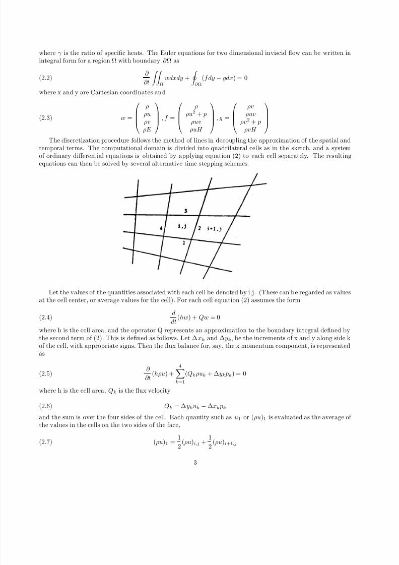
The discretization procedure follows the method of lines in decoupling the approximation of the spatial andtemporal terms. The computational domain is divided into quadrilateral cells as in the sketch, and a systemof ordinary differential equations is obtained by applying equation (2) to each cell separately. The resultingequations can then be solved by several alternative time stepping schemes.

Let the values of the quantities associated with each cell be denoted by i,j. (These can be regarded as valuesat the cell center, or average values for the cell). For each cell equation (2) assumes the form

d

dt(hw) + Qw = 0(2.4)

where h is the cell area, and the operator Q represents an approximation to the boundary integral defined bythe second term of (2). This is defined as follows. Let ∆xk and ∆yk, be the increments of x and y along side kof the cell, with appropriate signs. Then the flux balance for, say, the x momentum component, is representedas

∂

∂t(hρu) +

4k=1

(Qkρuk + ∆yk pk) = 0(2.5)

where h is the cell area, Qk is the flux velocity

Qk = ∆ykuk −∆xk pk(2.6)

and the sum is over the four sides of the cell. Each quantity such as u1 or (ρu)1 is evaluated as the average of the values in the cells on the two sides of the face,

(ρu)1 =1

2(ρu)i,j +

1

2(ρu)i+1,j(2.7)

3



for example. The scheme reduces to a central difference scheme on a Cartesian grid, and is second order accurateprovided that the grid is smooth enough.

3 Dissipative Terms

To suppress the tendency for odd and even point decoupling, and to prevent the appearance of wiggles in regionscontaining severe pressure gradients in the neighborhood of shock waves or stagnation points, it proves necessaryto augment the finite volume scheme by the addition of artificial dissipative terms, Therefore equation(4) isreplaced by the equation.

d

dt(hw) + Qw −Dw = 0(3.8)

where Q is the spatial discretization operator defined by equations(5-7), and D is a dissipative operator. Ex-tensive numerical experiments have established that an effective form for Dw is a blend of second and fourthdifferences with coefficients which depend on the local pressure gradient.

The construction of the dissipative terms for each of the four dependent variables is similar. For the densityequation

Dρ = Dxρ + Dyρ(3.9)

where Dxρ and Dyρ are corresponding contributions for the two coordinate directions, written in conservationform

Dxρ = di+ 1

2,j − di− 1

2,j

Dyρ = di,j+ 1

2

− di,j− 1

2

(3.10)

The terms on the right all have a similar form:

di+ 1

2,j =

hi+ 1

2,j

∆t

ε(2)

i+ 1

2,j

(ρi+1,j − ρi,j)− ε(4)

i+ 1

2,j

(ρi+2,j − 3ρi+1,j + 3ρi,j − ρi−1,j )

(3.11)

where h is the cell volume, and the coefficients ε(2) and ε(4) are adapted to the flow. Define

ν i,j =| pi+1,j − 2 pi,j + pi−1,j || pi+1,j | + 2 | pi,j |+ | pi−1,j |(3.12)

Then

(2)

i+ 1

2,j

= κ(2) max(ν i+1,j , ν i,j)(3.13)

and

(4)

i+ 1

2,j

= max

0, (κ(4) − ε(2)

i+ 1

2,j

)

(3.14)

where typical values of the constants κ(2) and κ(4) are

κ(2) = 14

, κ(4) = 1256

The dissipative terms for the remaining equations are obtained by substituting ρu, ρv and either ρE or ρH forρ in these formulas.

4



The scaling h/∆t in equation (11) conforms to the inclusion of the cell area h in the dependent variables of equation (8). Since equation (11) contains undivided differences, it follows that if ε(2) = O(∆x2) and ε(4) = O(1),then the added terms are of order ∆x3. This will be the case in a region where the flow is smooth. Near a shockwave ε(2) = O(1), and the scheme behaves locally like a first order accurate scheme.

It has been found that in smooth regions of the flow, the scheme is not sufficiently dissipative unless the fourth

differences are included, with the result that calculations will generally not converge to a completely steadystate. Instead, after they have reached an almost steady state, oscillations of very low amplitude continue indefinitely (with ∂ρ

∂t∼ 103, for example). These appear to be induced by reflections from the boundaries of

the computational domain. Near shock waves it has been found that the fourth differences tend to induceovershoots, and therefore they are switched off by subtracting ε(2) from κ(4) in equation (14).

4 Time Stepping Schemes

Stable time stepping methods for equation (6) can be patterned on standard schemes for ordinary differentialequations. Multistage two level schemes of the Runge Kutta type have the advantage that they do not requireany special starting procedure, in contrast to leap frog and Adams Bashforth methods, for example. The extrastages can be used either

1. to improve accuracy, or

2. to extend the stability region.

An advantage of this approach is that the properties of these schemes have been widely investigated, and arereadily available in textbooks on ordinary differential equations.

Consider a linear system of equations

dw

dt+ Aw = 0

Suppose that A can be expressed as A = T ΛT −1 where T is the matrix of the eigenvectors of A, and Λ is

diagonal. Then setting v = V −1

w yields separate equationsd

dtvk + λkvk = 0

for each dependent variable vk. The stability region is that region of the complex plane containing values of λ∆t for which the scheme is stable. Consider now the model problem

∂u

∂t+ a

∂u

∂x+ ε∆x

∂ 2u

∂x2= 0(4.15)

on a uniform mesh with interval ∆x, with a dissipative term of order ∆x. This can be reduced to a system of

ordinary differential equations by introducing central-difference approximations for ∂ ∂x

and ∂ 2

∂x2:

duj

dt +

a

∆x (ui+1 − ui−

1) +

ε

∆x (ui+1 − 2ui + ui−

1) = 0

Taking the Fourier transform in space

u =1

2π

∞

−∞

ueiωxdx

this becomes

5



du

dt+ λu = 0

where

λ =

1

∆x

ia sin(ω∆x)− 4ε sin2ω∆x

2

It can be seen that the maximum allowable value of the imaginary part of λ∆t determines the maximum valueof the Courant number a ∆t

∆xfor which the calculation will be stable, while the addition of the dissipative term

shifts the region of interest to the left of the imaginary axis.

In the present case, if the grid is held fixed in time so that the cell area h is constant, the system of equations(8) has the form

dw

dt+ P w = 0(4.16)

where if Q is the discretization operator defined in Section 2, and D is the dissipative operator defined in Section3, the nonlinear operator P is defined as

P w ≡ 1

h(Qw −Dw)(4.17)

The investigation has concentrated on two time stepping schemes. The first is a three stage scheme whichis defined as follows. Let a superscript n denote the time level, and let ∆t be the time step. Then at time leveln set

w(0) = wn

w(1) = w(0) −∆tP w(0)

w(2) = w(0) − ∆t2 (P w(0) + P w(1))

w(3) = w(0) − ∆t2 (P w(0) + P w(2))

wn+1 = w(3)

(4.18)

Variations of this scheme have been proposed by Gary[5], Stetter[6], and Graves and Johnson[10]. It canbe regarded as a Crank Nicolson scheme with a fixed point iteration to determine the solution at time leveln+1, and the iterations terminated after the third iteration. It is second order accurate in time, and for themodel problem [15] with ε = 0, it is stable when the Courant number schemes, this scheme gives up third orderaccuracy in time for a larger bound on the Courant number.a∆t

∆x

≤ 2

This bound is not increased by additional iterations. Compared with standard third order Runge-Kutta schemes,this scheme gives up third order accuracy in time for a larger bound on Courant number.

The other scheme which has been extensively investigated is the classical fourth order Runge-Kutta scheme,defined as follows. At time level n set

w(0) = wn

w(1) = w(0) − ∆t2

P w(0)

w(2) = w(0) − ∆t2 P w(1)

w(3) = w(0) −∆tP w(2)

w(4) = w(0) − ∆t6

P w(0) + 2P w(1) + 2P w(2) + P w(3)

wn+1 = w(4)

(4.19)

6





5 Boundary Conditions

Improper treatment of the boundary conditions can lead to serious errors and perhaps instability. In order totreat the flow exterior to a profile one must introduce an artificial outer boundary to produce a bounded domain.If the flow is subsonic at infinity there will be three incoming characteristics where there is inflow across theboundary, and one outgoing characteristic, corresponding to the possibility of escaping acoustic waves. Where

there is outflow, on the other hand, there will be three outgoing characteristics and one incoming characteristic.According to the theory of Kreiss[12], three conditions may therefore be specified at inflow, and one at outflow,while the remaining conditions are determined by the solution of the differential equation. It is not correct tospecify free stream conditions at the outer boundary.

For the formulation of the boundary conditions it is convenient to assume a local transformation to coordinatesX and Y such that the boundary coincides with a line Y constant. Using subscripts X and Y to denotederivatives, the Jacobian

h = xX

yY − x

Y yX

(5.21)

corresponds to the cell area of the finite volume scheme. Introduce the transformed flux vectors.

F = yY f − xY g, G = xXg − yXf (5.22)where f and g are defined by equation (3). In differential form equation(2) then becomes

∂

∂t(hw) +

∂F

∂X +

∂G

∂Y = 0(5.23)

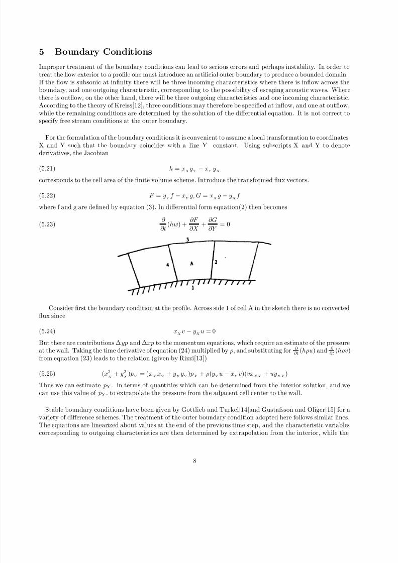
Consider first the boundary condition at the profile. Across side 1 of cell A in the sketch there is no convectedflux since

xX

v − yX

u = 0(5.24)

But there are contributions ∆yp and ∆xp to the momentum equations, which require an estimate of the pressureat the wall. Taking the time derivative of equation (24) multiplied by ρ, and substituting for ∂

∂t(hρu) and ∂

∂t(hρv)

from equation (23) leads to the relation (given by Rizzi[13])

(x2X

+ y2X

) pY

= (xX

xY

+ yX

yY

) pX

+ ρ(yY

u− xY

v)(vxXX

+ uyXX

)(5.25)

Thus we can estimate pY . in terms of quantities which can be determined from the interior solution, and we

can use this value of pY . to extrapolate the pressure from the adjacent cell center to the wall.

Stable boundary conditions have been given by Gottlieb and Turkel[14]and Gustafsson and Oliger[15] for avariety of difference schemes. The treatment of the outer boundary condition adopted here follows similar lines.The equations are linearized about values at the end of the previous time step, and the characteristic variablescorresponding to outgoing characteristics are then determined by extrapolation from the interior, while the

8



remaining boundary conditions are specified in a manner consistent with the conditions imposed by the freestream. Let

A =∂F

∂w, B =

∂G

∂w

Since the boundary is a line Y=constant, the eigenvalues of B determine the incoming and outgoing charac-

teristics. If qt and qn are the velocity components normal and tangential to the boundary, and c is the speed of sound, these eigenvalues are qn, qt, qn− c, andqn + c. Let values at the end of the previous time step be denotedby the subscript o, and let T o be the eigenvector matrix of B . Then Bo is reduced to diagonal form by thetransformation Λo = T −1o BoT o, and setting v = T −1o w, the linearized equation assumes the form

∂

∂t(hv) + T −1o AoT o

∂v

∂X + Λo

∂v

∂Y = 0

The characteristic variables are the components of v. These are p− c2oρ, qt, p− ρocoqn and po + ρocoqn

Let values extrapolated from the interior and free stream values be denoted by the subscripts e and ∞. Thenat the inflow boundary we set

p− c2oρ = p∞ − c

2oρqt = q∞

p− ρocoqn = p∞ − ρocoqn∞ p + ρocoqn = pe + ρocoqne

(5.26)

yielding

q =1

2( pe + p∞ + ρoco(qne − qn∞))

qn = qn∞ +p− p∞

ρ0c0

The density can be determined from (26a). For steady state calculations it can alternatively be determined byspecifying that the total enthalpy H has its free stream value.

At the outflow boundary one condition should be specified. If the flow is a parallel stream then ∂p∂y

= 0, sofor an open domain

p = p∞(5.27)

A non reflecting boundary condition which would eliminate incoming waves is

∂

∂t( p− ρocoqn) = 0(5.28)

This does not assure (27). Following Rudy and Strikwerda(16), (27) and (28) are therefore combined as

∂

∂t

( p

−ρocoqn) + α( p

− p∞) = 0(5.29)

where a typical value of the parameter α is 1/8. The velocity components and energy are extrapolated from theinterior.

Various other boundary conditions designed to reduce reflections from the outer boundary have been proposedby several authors (17, 18), and it seems that it would be worth while to test some of these alternatives.

9



6 Convergence Acceleration

Two devices have been used to accelerate the convergence of the solutions to a steady state. The first is to usethe largest possible time step permitted by the local stability bound everywhere In the computational domain.This has the effect of assuring that disturbances are propagated the whole way across the domain in a numberof time steps of the same order as the number of mesh intervals. It can be regarded as scaling the wave speed

to give equations of the form

∂w

∂t+ λ

∂f

∂x+

∂g

∂y

= 0

where λ is proportional to the local mesh interval. Assuming that a stretched grid is used to extend thecomputational domain away from the profile, λ will be very large near the outer edge of the domain.

As a model for this procedure consider the wave equation in polar coordinates r and θ.

φtt = c2

1

r

∂

∂r(rφr) +

1

r2φθθ

Suppose that the wave speed c is proportional to the radius, say c = αr. Then

φtt = α2

r

∂

∂r(rφr) + φθθ

This has solutions of the form

φ =1

rne−αnt

suggesting the possibility of exponential decay.

A more sophisticated modification of the equations, which is presently being investigated, is to set

∂w

∂t + M ∂f

∂x +

∂g

∂y

= 0

where the matrix M couples the equations for ρ,ρu,ρv, andρE , and modifies the eigenvalues of the system.

The second device for convergence acceleration is to introduce a forcing term proportional to the differencebetween the total enthalpy H and its free stream value H ∞. In a steady flow with a uniform free streamH = H ∞throughout the domain. The density and energy equations

∂

∂x(ρu) +

∂

∂y(ρv) = 0

and

∂

∂x (ρuH ) +∂

∂y (ρvH ) = 0

are then consistent. This property is not preserved by various predictor corrector difference schemes, such asthe MacCormack scheme. It is preserved by the schemes defined in sections 2-4, however, provided that thedissipative operator is applied to ρH and not ρE in the energy equation. Thus a forcing term proportional toH −H ∞ does not alter the steady state.

10



The reason for introducing such a term is to provide additional damping. The term is intended to have aneffect similar to that of the term containing φt in the telegraph equation:

φtt + αφt = φxx + φyy

Multiplying this equation by φt, and integrating by parts over all space leads to the relation

∂P

∂t+ α

∞

−∞

∞

−∞

φ2t dxdy = 0

where

P =1

2

∞

−∞

∞

−∞

(φ2t + φ2x + φ2y)dxdy

Since P is non negative, it must decay if α > 0 until φt = 0. When relaxation methods are regarded as simulatingtime dependent equations, it is similarly found that the term containing φt plays a critical role in determiningthe rate of convergence[19].

In subsonic flow the Euler equations are equivalent to the unsteady potential flow equation

φtt + 2uφxt + 2vφyt = (c2 − u2)φxx − 2uvφxy + (c2 − v2)φyy(6.30)

which can be reduced to the wave equation by introducing moving coordinates x = x − ut,y = y − vt. Alsothe unsteady Bernoulli equation is

φt + H = H ∞

It can be verified that if the Euler equations are written in primitive form, and the density equation is modifiedby the addition of a term proportional to H −H ∞, so that it becomes

∂ρ

∂t+ u

∂ρ

∂x+ v

∂ρ

∂v+ ρ

∂u

∂x+

∂v

∂y

+ αρ(H −H ∞) = 0

then the flow remains irrotational in the absence of shock waves, and equation (30) is modified by a termproportional to φt. When the density equation is combined with the momentum equations to yield a system of equations in conservation form, the modified equations become

∂ρ∂t

+ ∂ ∂x

(ρu) + ∂ ∂y

(ρv) + αρ(H −H ∞) = 0∂ ∂t

(ρu) + ∂ ∂x

(ρu2 + p) + ∂ ∂y

(ρvu) + αρu(H −H ∞) = 0∂ ∂t

(ρu) + ∂ ∂y

(ρuv) + ∂ ∂x

(ρv2 + p) + αρv(H −H ∞) = 0∂ ∂t

(ρE ) + ∂ ∂y

(ρuH ) + ∂ ∂x

(ρvH ) + αρH (H −H ∞) = 0

The energy equation now has a quadric term in H, like a Riccati equation. This can be destabilizing, and analternative which has been found effective in practice is to modify the energy equation to the form

∂

∂t (ρE ) +∂

∂x (ρuH ) +∂

∂y (ρvH ) + α(H −H ∞) = 0

which tends to drive H towards H ∞. The additional terms can conveniently be introduced in a separate fractionalstep at the end of each time step.

11



7 Results

Some typical results of numerical calculations are presented in this section. Since the purpose is primarily toshow the accuracy and convergence of the basic numerical algorithm, the examples are restricted to nonliftingflow past a cylinder and a NACA 0012 airfoil. Only the flow in the upper half plane was calculated, and an 0mesh was used with 64 intervals in the chord wise direction and 32 intervals in the normal direction. The mesh

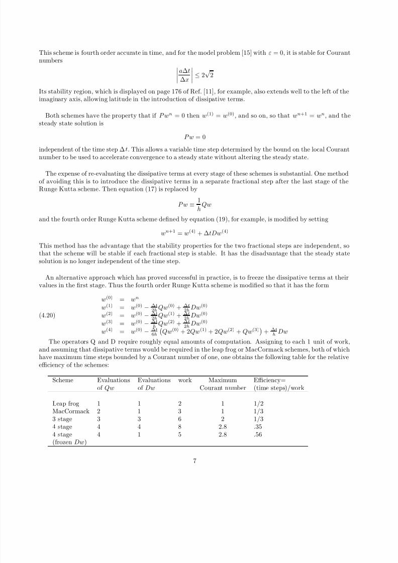
extended to a distance of about 25 chords from the profile, and the mesh interval near the outer boundary was of the order of a chord. In the case of the NACA 0012 airfoil, the cells adjacent to the outer boundary had an area2.5 million times greater than the area of the smallest cell, located at the trailing edge. Extensive numericalexperiments confirmed the superior efficiency of the modified fourth order Runge Kutta scheme defined byequation (20), and this scheme was used to produce all the results displayed in this section.

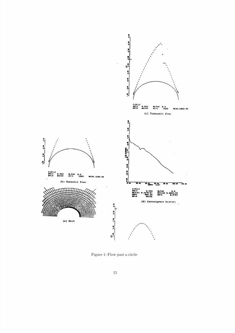
Figure 1 shows results for flow past a circular cylinder. The grid is displayed in Figure 1(a). Figures 1(b)and 1(c) show the computed pressure distributions for Mach numbers of .35 and .45. The flow is fully subsonicin the first case, and there should be no departure from fore and aft symmetry in an exact calculation. Theflow should also be isentropic. The calculations are normalized with p=1 and ρ=l at infinity, so the quantityS = p/ργ − 1 can be used as a measure of entropy generation. The largest computed value of S was .0003, ata point along the surface. At Mach .45 there is a moderately strong shock wave, as can be seen. The entropywas computed to be .0120 behind the shock wave. Figure 1(d) shows the convergence history for the flow at

Mach .45. The measure of convergence is the residual for the density, defined as the root mean square valueof ∂ρ

∂t(calculated at as ∆ρ/∆t for the complete time step). This was reduced from 1.67 to .486 10−9 in 1000

cycles. The mean rate of convergence was .978 per cycle. Another measure of convergence (not plotted) is theroot mean square deviation of the total enthalpy from its free strum value. This was reduced from .0828 to .50010−9. Enthalpy damping was used in this calculation to accelerate convergence. The calculation was startedimpulsively by suddenly introducing the cylindrical obstacle into a uniform flow, and immediately enforcing thesolid wall boundary condition at its surface. This creates very large disturbances, but the pattern of the flowfield is still quite rapidly established. One measure of this is the size of the supersonic zone. In this case thenumber of supersonic points was frozen after 450 cycles.

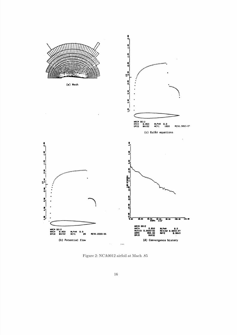
Figure 2 shows a comparison between the results of potential flow and Euler calculations for a NACA 0012airfoil at zero degrees angle of attack and Mach .850. The mesh is shown in Figure 2(a), the potential flow

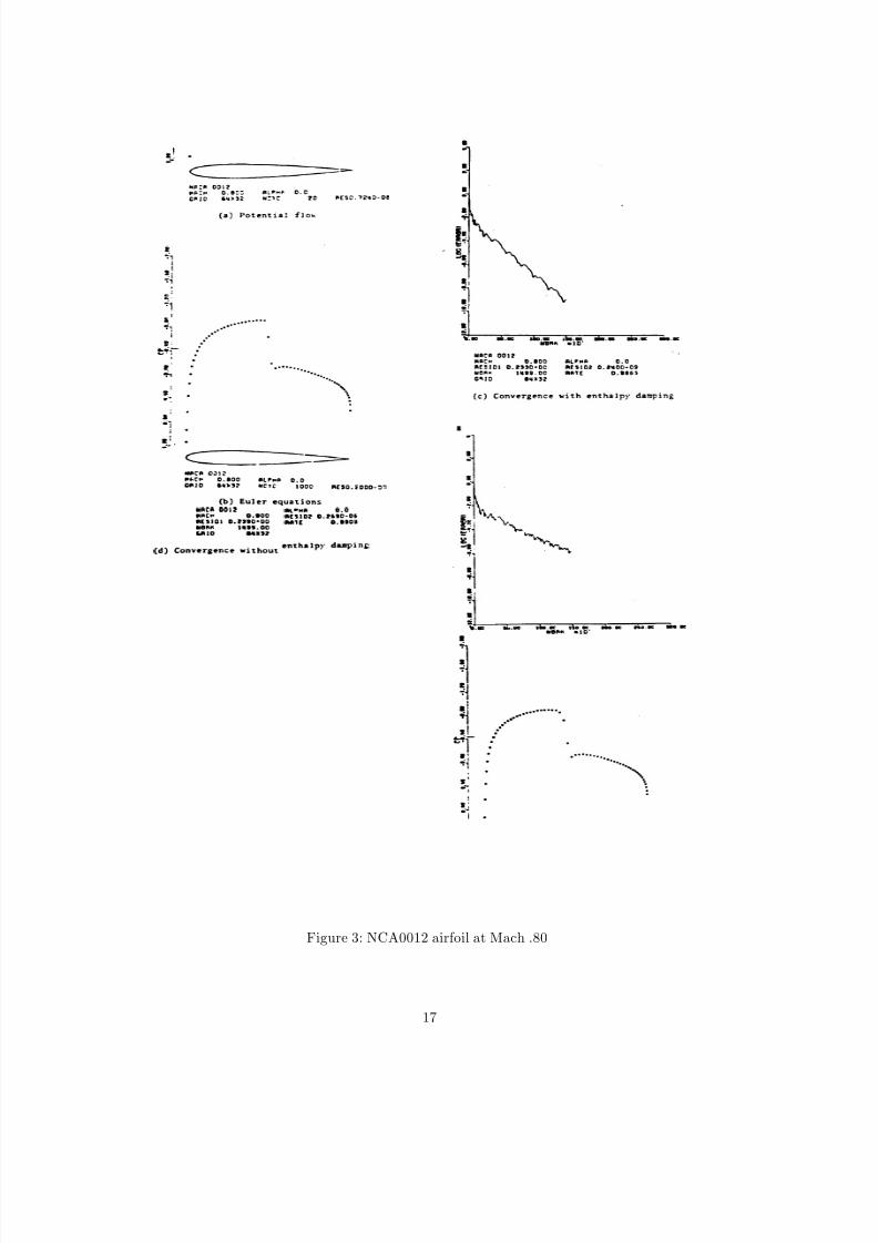
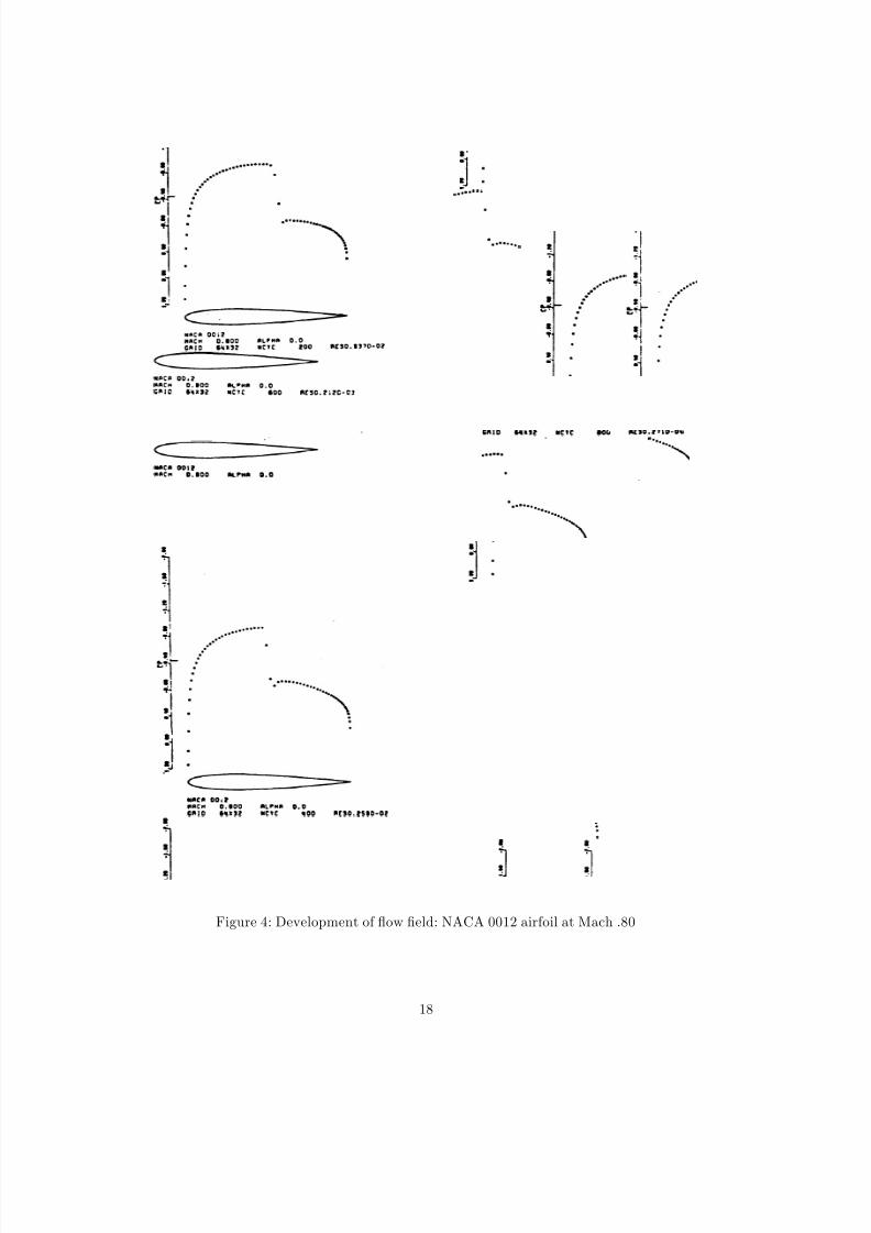
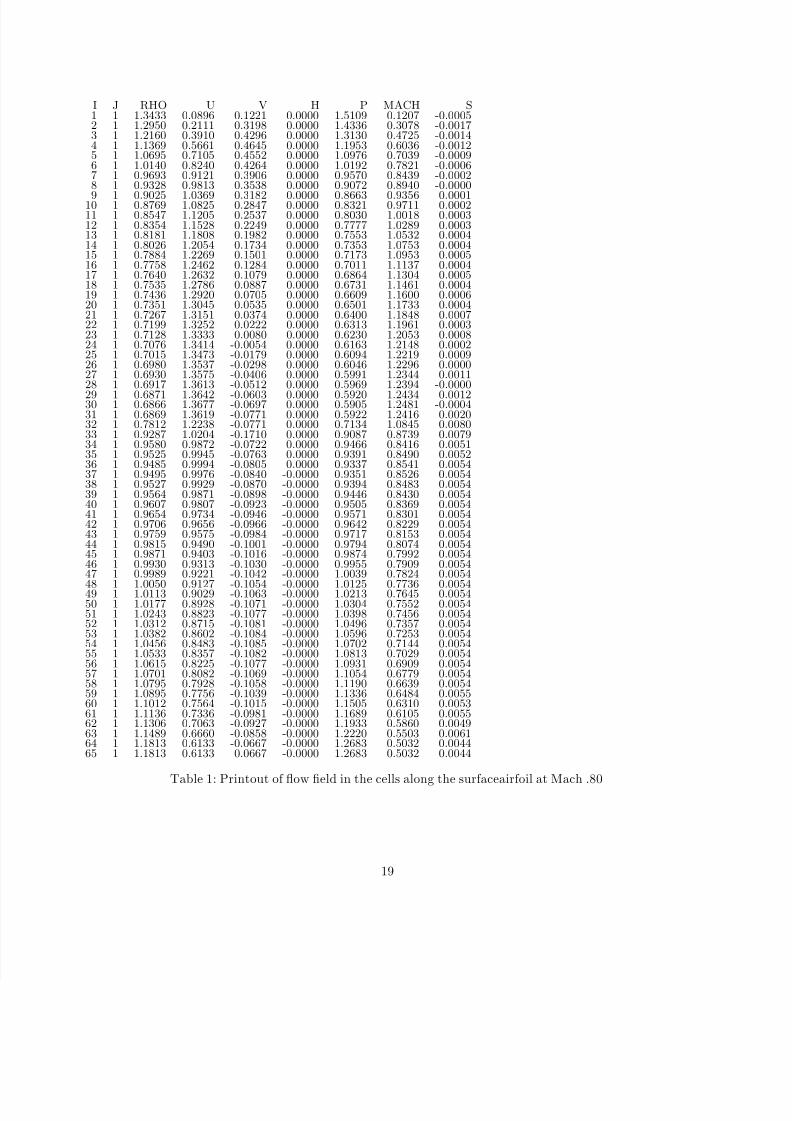
result is shown in Figure 2(b), and the Euler result is shown in Figure 2(c). It can be seen that the shockwave is further aft in the potential flow calculation, which was performed by the fully conservative finite volumemethod of Jameson and Caughey[20]. using a first order accurate formulation in the supersonic zone. Theconvergence history of the Euler calculation is shown in Figure 2(d). Figures 3(a) and 3(b) show a similarcomparison between the potential flow and Euler results for the NACA 0012 airfoil at Mach .900. In this casethe shock locations are identical. Figures 3(c) and 3(d) show the convergence history over 1500 cycles with andwithout enthalpy damping. Without enthalpy damping the final residual is .269 10−6. With enthalpy dampingit is .240 10−9. These runs used the potential flow result as the starting condition for the Euler calculation.Thus the flow pattern was already essentially established at the start of the Euler calculation, with the resultthat the number of points in the supersonic zone was frozen after 180 cycles when enthalpy damping was used.To illustrate the development of the flow field without the assistance of the potential flow calculation, Figure 4shows the result for the same flow after 200, 400, 600 and 800 cycles with an impulsive start. Finally a print outof the computed density, velocity components, total enthalpy, pressure, Mach number, and entropy (measured

as S = p/ργ

− 1) is displayed in Table 1. In an exact calculation S would be zero upstream of the shock wave.Actually it has a value of -.0017 near the leading edge. Then it settles to values in the range of .0002 to .0009ahead of the shock wave, and rises to .0054 behind the shock wave.

These results support the conclusions stated in the introduction. It also appears that shock waves can besatisfactorily captured without resorting to vector splitting and one sided differencing[21-24], at least for steady

12



state calculations, and that fairly rapid convergence to a steady state can be obtained without the use of animplicit scheme.

Attractive features of the scheme are its comparative simplicity, and its susceptibility to the extensive use of vector operations on a vector computer. The present implementation of the fourth order Runge Kutta schemerequires 426 floating point operations at each interior cell. On a mesh with 64x32 = 2048 cells a single cycle

therefore requires about .9 megaflops (million floating point operations). In tests on a Cray 1 computer it hasbeen found that the program operates at 44 cycles per second (corresponding to a computing speed of about40 megaflops per second). The code is written in standard FORTRAN, and this rate was achieved simply byrelying on the capability of the Cray FORTRAN computer to vectorize the code automatically. A still higherrate could be realized by writing certain critical segments of the program in assembly language. In practicea typical run is more than sufficiently converged for engineering applications within S00 cycles. At 44 cyclesa second such a calculation would be completed in 12 seconds, (or 24 seconds for a lifting case with twice asmany mesh cells to represent the flow in both the upper or lower half planes, provided that the same rate of convergence could be realized).

8 Acknowledgements

This work was supported by the Offic of Naval Research under Contract N00014-81-K-0379 and by NASA underContract NAG2-96.

References

[1] Jameson, A. ”Numerical Calculation of Transonic Flow with Shock Waves”, Symposium Transsonicum II,Gottingen. 1975, Springer-Verlag, 1976.

[2] Rizzi, A., and Viviand, H. (editors), ”Numerical Methods for the Computation of Inviscid Transonic Flow

with Shocks”, Proceedings of GA*’ Workshop, Stockholm, 1979, Viewveg Verlag, 1981.

[3] Steinhoff, J. and Jameson, A. ”Multiple Solutions of the Transonic Potential Flow Equation”, Fifth AIMComputational Fluid Dynamics Conference, Palo Alto, 1981.

[4] Rizzi, A. ”Computation of Rotational Transonic Flow, in Numerical Methods for the Computation of In-

viscid Transonic Flow with Shocks”, Proceedings of GAMM Workshop, Stockholm, 1979, Viewveg Verlag,1981.

[5] Gary, J. ”On Certain Finite Difference Schemes for Hyperbolic Systems”, Math. Comp.. Vol. 18, pp. 1-18,1964.

[6] Stetter, H.J. ”Improved Absolute Stability of Predictor-Corrector Schemes”, Computing, Vol. 3, pp. 286-296,1968.

[7] Rizzi, A. and Eriksson, L.E. ”Transfinite Mesh Generation and Damped Euler Equation Algorithr for Tran-

sonic Flow Around Wing-body Configurations”, Fifth AIAA Computational Fluid Dynamics Conference,Palo Alto, 1981.

[8] Viviand, H. ”Pseudo Unsteady Methods for Transonic Flow Computations”, Proceedings of Seventh Inter-national Conference on Numerical Methods in Fluid Dynamics, Stanford, 1960, Springer-Verlag, 1981.

[9] Jameson, A., Rizzi, A., Schmidt, W., and Whitfield. D. ”Finite Volume Solution for the Euler Equation

for Transonic Flow over Airfoils and Wings Including Viscous Effects”, AIAA Paper 81-1265, 1981.

13



[10] Graves, R. and Johnson, N. ”Navier Stokes Solutions Using Stetter’s Method”, AIAA Journal, Vol. 16, pp.1013-1015, 1978.

[11] Stetter, H.J. ”Analysis of Discretization Methods for Ordinary Differential Equations”, Springer-Verlag,1973.

[12] Kreiss, H.O. ”Initial Boundary Value Problems for Hyperbolic Systems”, Comm. Pure Appl. Math., Vol.23, pp. 277-298, 1970.

[13] Rizzi, A. ”Numerical Implementation of Solid Body Boundary Conditions for the Euler Equations”, ZAMMVol. S8, pp. 301-304, 1978.

[14] Gottlieb. D. and Turkel. E. ”Boundary Conditions for Multistep Finite Difference Methods for Time De-

pendent Equations”, J. Computational Physics, Vol. 26, pp. 181-196, 1978.

[15] Gustafsson, B. and Oliger, J. ”Stable Boundary Approximations for a Class of Time Discretizations of

ut = ADou”, Upsala University, Dept. of Computer Sciencgs, Report 87, 1990.

[16] Rudy, D. and Strikwerda, J. ”A Non-reflecting Outflow boundary Condition for Subsonic Navier Stokes

Calculations”, J. Computational Physics. Vol. 36, pp. SS-70, 1980.

[17] Engquist, B. and Majda, A. ”Absorbing Boundary Conditions for the Numerical Simulation of Waves”,Math. Comp. Vol. 31, pp. 629-651, 1977.

[18] Bayliss, A. and Turkel, E. ”Outflow boundary Conditions for Fluid Dynamics” ICASE Report 80-21, 1980.

[19] Garabedian, P.R. ”Estimation of the Relaxation Factor for Small Mesh Size” , Math Tables Aids Comp.,Vol. 10, pp. 183-185, 1956.

[20] Caughey, D. and Jameson, A. ”Basic Advances in the Finite Volume Method for Transonic Potential Flow

Calculations”, Symposium on Numerical and Physical Aspects of Aerodynamic Flows, Long Beach, 1981.

[21] Steger, J. and Warming, R. ”Flux Vector Splitting for the Inviscid Gas Dynamic Equations with Application

to Finite Difference Methods”, NASA TM 78605, 1979.

[22] Roe, P.L. ”The Use of the Riemann Problem in Finite Difference Schemes”, Proceedings of Seventh Inter-national Conference on Numerical Methods. in Fluid Dynamics, Stanford, 1980, Springer-Verlag, 1981.

[23] Roe, P.L. ”Numerical Algorithms for the Linear Wave Equation”, Royal Aircraft Establishment Memoran-dum, 1980.

[24] Van Leer, B. ”Towards the Ultimate Conservative Differencing Scheme, V, A Second Order Sequel to

Godunov’s Method”, J. Computational Physics, Vol. 32, pp. 101-126, 1979.

14



Figure 1: Flow past a circle

15



Figure 2: NCA0012 airfoil at Mach .85

16



Figure 3: NCA0012 airfoil at Mach .80

17



Figure 4: Development of flow field: NACA 0012 airfoil at Mach .80

18



I J RHO U V H P MACH S1 1 1.3433 0.0896 0.1221 0.0000 1.5109 0.1207 -0.00052 1 1.2950 0.2111 0.3198 0.0000 1.4336 0.3078 -0.00173 1 1.2160 0.3910 0.4296 0.0000 1.3130 0.4725 -0.00144 1 1.1369 0.5661 0.4645 0.0000 1.1953 0.6036 -0.00125 1 1.0695 0.7105 0.4552 0.0000 1.0976 0.7039 -0.00096 1 1.0140 0.8240 0.4264 0.0000 1.0192 0.7821 -0.00067 1 0.9693 0.9121 0.3906 0.0000 0.9570 0.8439 -0.00028 1 0.9328 0.9813 0.3538 0.0000 0.9072 0.8940 -0.0000

9 1 0.9025 1.0369 0.3182 0.0000 0.8663 0.9356 0.000110 1 0.8769 1.0825 0.2847 0.0000 0.8321 0.9711 0.000211 1 0.8547 1.1205 0.2537 0.0000 0.8030 1.0018 0.000312 1 0.8354 1.1528 0.2249 0.0000 0.7777 1.0289 0.000313 1 0.8181 1.1808 0.1982 0.0000 0.7553 1.0532 0.000414 1 0.8026 1.2054 0.1734 0.0000 0.7353 1.0753 0.000415 1 0.7884 1.2269 0.1501 0.0000 0.7173 1.0953 0.000516 1 0.7758 1.2462 0.1284 0.0000 0.7011 1.1137 0.000417 1 0.7640 1.2632 0.1079 0.0000 0.6864 1.1304 0.000518 1 0.7535 1.2786 0.0887 0.0000 0.6731 1.1461 0.000419 1 0.7436 1.2920 0.0705 0.0000 0.6609 1.1600 0.000620 1 0.7351 1.3045 0.0535 0.0000 0.6501 1.1733 0.000421 1 0.7267 1.3151 0.0374 0.0000 0.6400 1.1848 0.000722 1 0.7199 1.3252 0.0222 0.0000 0.6313 1.1961 0.000323 1 0.7128 1.3333 0.0080 0.0000 0.6230 1.2053 0.000824 1 0.7076 1.3414 -0.0054 0.0000 0.6163 1.2148 0.000225 1 0.7015 1.3473 -0.0179 0.0000 0.6094 1.2219 0.000926 1 0.6980 1.3537 -0.0298 0.0000 0.6046 1.2296 0.000027 1 0.6930 1.3575 -0.0406 0.0000 0.5991 1.2344 0.001128 1 0.6917 1.3613 -0.0512 0.0000 0.5969 1.2394 -0.000029 1 0.6871 1.3642 -0.0603 0.0000 0.5920 1.2434 0.001230 1 0.6866 1.3677 -0.0697 0.0000 0.5905 1.2481 -0.000431 1 0.6869 1.3619 -0.0771 0.0000 0.5922 1.2416 0.002032 1 0.7812 1.2238 -0.0771 0.0000 0.7134 1.0845 0.008033 1 0.9287 1.0204 -0.1710 0.0000 0.9087 0.8739 0.007934 1 0.9580 0.9872 -0.0722 0.0000 0.9466 0.8416 0.005135 1 0.9525 0.9945 -0.0763 0.0000 0.9391 0.8490 0.005236 1 0.9485 0.9994 -0.0805 0.0000 0.9337 0.8541 0.005437 1 0.9495 0.9976 -0.0840 -0.0000 0.9351 0.8526 0.005438 1 0.9527 0.9929 -0.0870 -0.0000 0.9394 0.8483 0.005439 1 0.9564 0.9871 -0.0898 -0.0000 0.9446 0.8430 0.005440 1 0.9607 0.9807 -0.0923 -0.0000 0.9505 0.8369 0.005441 1 0.9654 0.9734 -0.0946 -0.0000 0.9571 0.8301 0.005442 1 0.9706 0.9656 -0.0966 -0.0000 0.9642 0.8229 0.005443 1 0.9759 0.9575 -0.0984 -0.0000 0.9717 0.8153 0.005444 1 0.9815 0.9490 -0.1001 -0.0000 0.9794 0.8074 0.005445 1 0.9871 0.9403 -0.1016 -0.0000 0.9874 0.7992 0.005446 1 0.9930 0.9313 -0.1030 -0.0000 0.9955 0.7909 0.005447 1 0.9989 0.9221 -0.1042 -0.0000 1.0039 0.7824 0.0054

48 1 1.0050 0.9127 -0.1054 -0.0000 1.0125 0.7736 0.005449 1 1.0113 0.9029 -0.1063 -0.0000 1.0213 0.7645 0.005450 1 1.0177 0.8928 -0.1071 -0.0000 1.0304 0.7552 0.005451 1 1.0243 0.8823 -0.1077 -0.0000 1.0398 0.7456 0.005452 1 1.0312 0.8715 -0.1081 -0.0000 1.0496 0.7357 0.005453 1 1.0382 0.8602 -0.1084 -0.0000 1.0596 0.7253 0.005454 1 1.0456 0.8483 -0.1085 -0.0000 1.0702 0.7144 0.005455 1 1.0533 0.8357 -0.1082 -0.0000 1.0813 0.7029 0.005456 1 1.0615 0.8225 -0.1077 -0.0000 1.0931 0.6909 0.005457 1 1.0701 0.8082 -0.1069 -0.0000 1.1054 0.6779 0.005458 1 1.0795 0.7928 -0.1058 -0.0000 1.1190 0.6639 0.005459 1 1.0895 0.7756 -0.1039 -0.0000 1.1336 0.6484 0.005560 1 1.1012 0.7564 -0.1015 -0.0000 1.1505 0.6310 0.005361 1 1.1136 0.7336 -0.0981 -0.0000 1.1689 0.6105 0.005562 1 1.1306 0.7063 -0.0927 -0.0000 1.1933 0.5860 0.004963 1 1.1489 0.6660 -0.0858 -0.0000 1.2220 0.5503 0.006164 1 1.1813 0.6133 -0.0667 -0.0000 1.2683 0.5032 0.004465 1 1.1813 0.6133 0.0667 -0.0000 1.2683 0.5032 0.0044

Table 1: Printout of flow field in the cells along the surfaceairfoil at Mach .80

19

Documents

numerical solution of euler equation