Embed Size (px)
Citation preview

Page | 1
Chapter 5
Numerical Solutions of Algebraic and Transcendental Equations
5.1 Introduction
An expression of the form 𝑓 𝑥 = 𝑎0𝑥𝑛+𝑎1𝑥
𝑛−1 + ⋯ + 𝑎𝑛−1𝑥 + 𝑎𝑛 , 𝑎0 ≠ 0 is
called a polynomial of degree ‘𝑛’and the polynomial 𝑓 𝑥 = 0 is called an algebraic
equation of 𝑛𝑡ℎ degree.If 𝑓 𝑥 contains trigonometric, logarithmic or exponential
functions, then 𝑓 𝑥 = 0 is called a transcendental equation. For example 𝑥2 +2 sin 𝑥 + 𝑒𝑥 = 0 is a transcendental equation.
If 𝑓 𝑥 is an algebraic polynomial of degree less than or equal to 4, direct methods for
finding the roots of such equation are available. But if 𝑓 𝑥 is of higher degree or it
involves transcendental functions, direct methods do not exist and we need to apply
numerical methods to find the roots of the equation 𝑓 𝑥 = 0.
Some useful results
If 𝛼 is root of the equation 𝑓 𝑥 = 0, then 𝑓 𝛼 = 0 Every equation of 𝑛𝑡ℎdegree has exactly 𝑛 roots (real or imaginary)
Intermediate Value Theorem: If 𝑓 𝑥 is a continuous function in a closed
interval 𝑎, 𝑏 and 𝑓 𝑎 &𝑓 𝑏 are having opposite signs, then the equation
𝑓 𝑥 = 0 has atleast one real root or odd number of roots between 𝑎and 𝑏.
If 𝑓 𝑥 is a continuous function in the closed interval 𝑎, 𝑏 and 𝑓 𝑎 & 𝑓 𝑏
are of same signs, then the equation 𝑓 𝑥 = 0 has no root or even number of
roots between 𝑎and 𝑏.
5.2Numerical methods to find roots of algebraic and transcendental equations
Most numerical methods use iterative procedures to find an approximate root of an
equation 𝑓 𝑥 = 0. They require an initial guess of the root as starting value and each
subsequent iteration leads closer to the actual root.
Order of convergence: For any iterative numerical method, each successive iteration
gives an approximation that moves progressively closer to actual solution. This is known
as convergence. Any numerical method is said have order of convergence 𝜌, if 𝜌 is the
largest positive number such that 𝜖𝑛+1 ≤ 𝑘 𝜖𝑛 𝜌 , where 𝜖𝑛 and 𝜖𝑛+1 are errors in
𝑛𝑡ℎand (𝑛 + 1)𝑡ℎ iterations, 𝑘 is a finite positive constant.

Page | 2
5.2.1 Bisection Method (or Bolzano Method) Bisection method is used to find an
approximate root in an interval by repeatedly
bisecting into subintervals. It is a very simple
and robust method but it is also relatively
slow. Because of this it is often used to obtain
a rough approximation to a solution which is
then used as a starting point for more rapidly
converging methods. This method is based on
the intermediate value theorem for continuous
functions.
Algorithm:
Let 𝑓 𝑥 be a continuous function in the interval 𝑎, 𝑏 , such that 𝑓 𝑎 and 𝑓 𝑏 are of
opposite signs, i.e. 𝑓 𝑎 . 𝑓 𝑏 < 0.
Step1. Take the initial approximation given by 𝑥0 =𝑎+𝑏
2, one of the three conditions
arises for finding the 1st approximation 𝑥1
i. 𝑓(𝑥0) = 0, we have a root at 𝑥0.
ii. If 𝑓 𝑎 . 𝑓 𝑥0 < 0, the root lies between 𝑎 and 𝑥0 ∴ 𝑥1 =𝑎+ 𝑥0
2 and repeat the
procedure by halving the interval again.
iii. I𝑓 𝑓 𝑏 . 𝑓 𝑥0 < 0, the root lies between 𝑥0 and 𝑏 ∴ 𝑥1 = 𝑥0+𝑏
2 and repeat the
procedure by halving the interval again.
iv. Continue the process until root is found to be of desired accuracy.
Remarks:
Convergence is not unidirectional as none of the end points is fixed. As a result
convergence of Bisection method is very slow.
Repeating the procedure 𝑛 times, the new interval will be exactly half the length of
the previous one, until the root is found of desired accuracy (error less than ∈). ∴
and at the end of𝑛𝑡ℎ iteration, the interval containing the root will be of length 𝑏−𝑎
2𝑛, such that
𝑏−𝑎
2𝑛<∈
⇒ log 𝑏−𝑎
2𝑛< log ∈
⇒ log 𝑏 − 𝑎 − log 2𝑛 < log ∈
⇒ log 𝑏 − 𝑎 − log ∈ < 𝑛 log 2
⇒ 𝑛 >log 𝑏−𝑎 −log ∈
log 2
Page | 3
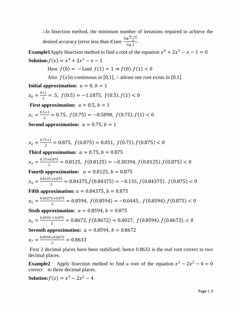
∴In bisection method, the minimum number of iterations required to achieve the
desired accuracy (error less than ∈)are log
𝑏−𝑎
∈
log 2.
Example1Apply bisection method to find a root of the equation 𝑥4 + 2𝑥3 − 𝑥 − 1 = 0
Solution:𝑓 𝑥 = 𝑥4 + 2𝑥3 − 𝑥 − 1
Here 𝑓 0 = −1and 𝑓 1 = 1 ⇒ 𝑓 0 . 𝑓 1 < 0
Also 𝑓 𝑥 is continuous in 0,1 , ∴ atleast one root exists in 0,1
Initial approximation: 𝑎 = 0, 𝑏 = 1
𝑥0 =0+1
2= .5, 𝑓 0.5 = −1.1875, 𝑓 0.5 . 𝑓 1 < 0
First approximation: 𝑎 = 0.5, 𝑏 = 1
𝑥1 =0.5+1
2= 0.75, 𝑓 0.75 = −0.5898, 𝑓 0.75 . 𝑓 1 < 0
Second approximation: 𝑎 = 0.75, 𝑏 = 1
𝑥2 =0.75+1
2= 0.875, 𝑓 0.875 = 0.051, 𝑓 0.75 . 𝑓 0.875 < 0
Third approximation: 𝑎 = 0.75, 𝑏 = 0.875
𝑥3 =0.75+0.875
2= 0.8125, 𝑓 0.8125 = −0.30394, 𝑓 0.8125 . 𝑓 0.875 < 0
Fourth approximation: 𝑎 = 0.8125, 𝑏 = 0.875
𝑥4 =0.8125+0.875
2= 0.84375,𝑓 0.84375 = −0.135, 𝑓 0.84375 . 𝑓 0.875 < 0
Fifth approximation: 𝑎 = 0.84375, 𝑏 = 0.875
𝑥5 =0.84375+0.875
2= 0.8594, 𝑓 0.8594 = −0.0445, . 𝑓 0.8594 . 𝑓 0.875 < 0
Sixth approximation: 𝑎 = 0.8594, 𝑏 = 0.875
𝑥6 =0.8594 + 0.875
2= 0.8672, 𝑓 0.8672 = 0.0027, 𝑓 0.8594 . 𝑓 0.8672 . < 0
Seventh approximation: 𝑎 = 0.8594, 𝑏 = 0.8672
𝑥7 =0.8594+0.8672
2= 0.8633
First 2 decimal places have been stabilized; hence 0.8633 is the real root correct to two
decimal places.
Example2 Apply bisection method to find a root of the equation 𝑥3 − 2𝑥2 − 4 = 0
correct to three decimal places.
Solution:𝑓 𝑥 = 𝑥3 − 2𝑥2 − 4

Page | 4
Here 𝑓 2 = −4 and 𝑓 3 = 5 ⇒ 𝑓 2 . 𝑓 3 < 0
Also 𝑓 𝑥 is continuous in 2,3 , ∴ atleast one root exists in 2,3
Initial approximation: 𝑎 = 2, 𝑏 = 3
𝑥0 =2+3
2= 2.5, 𝑓 2.5 = −1.8750, 𝑓 2.5 . 𝑓 3 < 0
First approximation: 𝑎 = 2.5, 𝑏 = 3
𝑥1 =2.5+3
2= 2.75, 𝑓 2.75 = 1.6719, 𝑓 2.5 . 𝑓 2.75 < 0
Second approximation: 𝑎 = 2.5, 𝑏 = 2.75
𝑥2 =2.5+2.75
2= 2.625, 𝑓 2.625 = 0.3066, 𝑓 2.5 . 𝑓 2.625 < 0
Third approximation: 𝑎 = 2.5, 𝑏 = 2.625
𝑥3 =2.5+2.625
2= 2.5625, 𝑓 2.5625 = −.3640, 𝑓 2.5625 . 𝑓 2.625 < 0
Fourth approximation: 𝑎 = 2.5625, 𝑏 = 2.625
𝑥4 =2.5625+2.625
2= 2.59375, 𝑓 2.59375 = −.0055, 𝑓 2.59375 . 𝑓 2.625 < 0
Fifth approximation: 𝑎 = 2.59375, 𝑏 = 2.625
𝑥5 =2.59375+2.625
2= 2.60938, 𝑓 2.60938 = .1488, 𝑓 2.59375 . 𝑓 2.60938 < 0
Sixth approximation: 𝑎 = 2.59375, 𝑏 = 2.60938
𝑥6 =2.59375+2.60938
2= 2.60157,𝑓 2.60157 = .0719, 𝑓 2.59375 . 𝑓 2.60157 < 0
Seventh approximation: 𝑎 = 2.59375, 𝑏 = 2.60157
𝑥7 =2.59375+2.60157
2= 2.59765, 𝑓 2.59765 = .0329, 𝑓 2.59375 . 𝑓 2.59765 < 0
Eighth approximation: 𝑎 = 2.59375, 𝑏 = 2.59765
𝑥8 =2.59375+2.59765
2= 2.5957, 𝑓 2.5957 = .0136, 𝑓 2.59375 . 𝑓 2.5957 < 0
Ninth approximation: 𝑎 = 2.59375, 𝑏 = 2.5957
𝑥9 =2.59375+2.5957
2= 2.5947, 𝑓 2.5947 = −.004, 𝑓 2.5947 . 𝑓 2.5957 < 0
Tenth approximation: 𝑎 = 2.5947, 𝑏 = 2.5957
𝑥10 =2.5947+2.5957
2= 2.5952
Hence 2.5952 is the real root correct to three decimal places.
Example3 Apply bisection method to find a root of the equation 𝑥𝑒𝑥 = 1 correct to
three decimal places.

Page | 5
Solution:𝑓 𝑥 = 𝑥𝑒𝑥 − 1
Here 𝑓 0 = −1 and 𝑓 1 = 𝑒 − 1 = 1.718 ⇒ 𝑓 0 . 𝑓 1 < 0
Also 𝑓 𝑥 is continuous in 0,1 , ∴ atleast one root exists in 0,1
Initial approximation: 𝑎 = 0, 𝑏 = 1
𝑥0 =0+1
2= 0.5, 𝑓 0.5 = −0.1756, 𝑓 0.5 . 𝑓 1 < 0
First approximation: 𝑎 = 0.5, 𝑏 = 1
𝑥1 =0.5+1
2= 0.75, 𝑓 0.75 = 0.5877, 𝑓 0.5 . 𝑓 0.75 < 0
Second approximation: 𝑎 = 0.5, 𝑏 = 0.625
𝑥2 =0.5+0.75
2= 0.625, 𝑓 0.625 = 0.8682, 𝑓 0.5 . 𝑓 0.625 < 0
Third approximation: 𝑎 = 0.5, 𝑏 = 0.625
𝑥3 =0.5+0.625
2= 0.5625, 𝑓 0.5625 = −0.0128, 𝑓 0.5625 . 𝑓 0.625 < 0
Fourth approximation: 𝑎 = 0.5625, 𝑏 = 0.625
𝑥4 =0.5625+0.625
2= 0.59375, 𝑓 0.59375 = 0.0751, 𝑓 0.5625 . 𝑓 0.59375 < 0
Fifth approximation: 𝑎 = 0.5625, 𝑏 = 0.59375
𝑥5 =0.5625+0.59375
2= 0.5781, 𝑓 0.5781 = 0.0305, 𝑓 0.5625 . 𝑓 0.5781 < 0
Sixth approximation: 𝑎 = 0.5625, 𝑏 = 0.5781
𝑥6 =0.5625+0.5781
2= 0.5703,𝑓 0.5703 = .0087, 𝑓 0.5625 . 𝑓 0.5703 < 0
Seventh approximation: 𝑎 = 0.5625, 𝑏 = 0.5703
𝑥7 =0.5625+0.5703
2= 0.5664, 𝑓 0.5664 = −.002, 𝑓 0.5664 . 𝑓 0.5703 < 0
Eighth approximation: 𝑎 = 0.5664, 𝑏 = 0.5703
𝑥8 =0.5664+0.5703
2= 0.5684, 𝑓 0.5684 = 0.0035, 𝑓 0.5664 . 𝑓 0.5684 < 0
Ninth approximation: 𝑎 = 0.5664, 𝑏 = 0.5684
𝑥9 =0.5664+0.5684
2= 0.5674, 𝑓 0.5674 = .0007, 𝑓 0.5664 . 𝑓 0.5674 < 0
Tenth approximation: 𝑎 = 0.5664, 𝑏 = 0.5674
𝑥10 =0.5664+0.5674
2= 0.5669, 𝑓 0.5669 = −.0007, 𝑓 0.5669 . 𝑓 0.5674 < 0
Eleventh approximation: 𝑎 = 0.5669, 𝑏 = 0.5674
𝑥11 =0.5669+0.5674
2= 0.56715, 𝑓 0.56715 = .00001~0

Page | 6
Hence 0.56715 is the real root correct to three decimal places.
Example4 Using bisection method find an approximate root of the equation sin 𝑥 =1
𝑥
correct to two decimal places.
Solution:𝑓 𝑥 = 𝑥sin 𝑥 − 1
Here 𝑓 1 = sin 1 − 1 = −0.1585 and 𝑓 2 = 2sin 2 − 1 = 0.8186
Also 𝑓 𝑥 is continuous in 1,2 , ∴ atleast one root exists in 1,2
Initial approximation: 𝑎 = 1, 𝑏 = 2
𝑥0 =1+2
2= 1.5, 𝑓 1.5 = 0.4963, 𝑓 1 . 𝑓 1.5 < 0
First approximation: 𝑎 = 1, 𝑏 = 1.5
𝑥1 =1+1.5
2= 1.25, 𝑓 1.25 = 0.1862, 𝑓 1 . 𝑓 1.25 < 0
Second approximation: 𝑎 = 1, 𝑏 = 1.25
𝑥2 =1+1.25
2= 1.125, 𝑓 1.125 = 0.0151, 𝑓 1 . 𝑓 1.125 < 0
Third approximation: 𝑎 = 1, 𝑏 = 1.125
𝑥3 =1+1.125
2= 1.0625, 𝑓 1.0625 = −0.0718, 𝑓 1.0625 . 𝑓 1.125 < 0
Fourth approximation: 𝑎 = 1.0625, 𝑏 = 1.125
𝑥4 =1.0625+1.125
2= 1.09375, 𝑓 1.09375 = −0.0284, 𝑓 1.09375 . 𝑓 1.125 < 0
Fifth approximation: 𝑎 = 1.09375, 𝑏 = 1.125
𝑥5 =1.09375+1.125
2= 1.10937, 𝑓 1.10937 = −0.0066, 𝑓 1.10937 . 𝑓 1.125 < 0
Sixth approximation: 𝑎 = 1.10937, 𝑏 = 1.125
𝑥6 =1.10937+1.125
2= 1.11719,𝑓 1.11719 = .0042, 𝑓 1.10937 . 𝑓 1.11719 < 0
Seventh approximation: 𝑎 = 1.10937, 𝑏 = 1.11719
𝑥7 =1.10937+1.11719
2= 1.11328, 𝑓 1.11328 = −.0012~0
Hence 1.11328 is the real root correct to two decimal places.
5.2.2 Regula- Falsi Method (Geometrical Interpretation) Regula-Falsi method is also known as method of false position as false position of curve
is taken as initial approximation. Let 𝑦 = 𝑓(𝑥) be represented by the curve 𝐴𝐵.The real
root of equation 𝑓 𝑥 = 0 is 𝛼 as shown in adjoining figure. The false position of curve
𝐴𝐵 is taken as chord 𝐴𝐵 and initial approximation 𝑥0 is the point of intersection of chord

Page | 7
𝐴𝐵 with 𝑥-axis. Successive approximations 𝑥1, 𝑥2 , …are given by point of intersection of
chord 𝐴′𝐵, 𝐴′′ 𝐵, …with 𝑥 − axis, until the root is found to be of desired accuracy.
Now equation of chord AB in two-point form is given by:
𝑦 − 𝑓 𝑎 =𝑓 𝑏 −𝑓 𝑎
𝑏−𝑎(𝑥 − 𝑎)
To find 𝑥0 (point of intersection of chord AB with 𝑥 -
axis), put 𝑦 = 0
⇒ −𝑓 𝑎 =𝑓 𝑏 −𝑓 𝑎
𝑏−𝑎 𝑥0 − 𝑎
⇒ (𝑥0 − 𝑎) = − 𝑏−𝑎 𝑓 𝑎
𝑓(𝑏)−𝑓(𝑎)
⇒ 𝑥0 = 𝑎 − 𝑏−𝑎
𝑓 𝑏 −𝑓 𝑎 𝑓(𝑎)
Repeat the procedure until the root is found to the desired
accuracy.
Remarks:
Rate of convergence is much faster than that of bisection method.
Unlike bisection method, one end point will converge to the actual root 𝑎 , whereas the other end point always remains fixed. As a result Regula- Falsi
method has linear convergence.
Example5 Apply Regula-Falsi method to find a root of the equation 𝑥3 + 𝑥 − 1 =0 correct to two decimal places.
Solution:𝑓 𝑥 = 𝑥3 + 𝑥 − 1
Here 𝑓 0 = −1 and 𝑓 1 = 1 ⇒ 𝑓 0 . 𝑓 1 < 0
Also 𝑓 𝑥 is continuous in 0,1 , ∴ atleast one root exists in 0,1
Initial approximation:𝑥0 = 𝑎 − 𝑏−𝑎
𝑓 𝑏 −𝑓 𝑎 𝑓(𝑎) ; 𝑎 = 0, 𝑏 = 1
⇒ 𝑥0 = 0 − 1−0
𝑓 1 −𝑓 0 𝑓 0 = 0 −
1
1− −1 (−1) = 0.5
𝑓 0.5 = −0.375, 𝑓 0.5 . 𝑓 1 < 0
First approximation: 𝑎 = 0.5, 𝑏 = 1
𝑥1 = 0.5 − 1−0.5
𝑓 1 −𝑓 0.5 𝑓 0.5 = 0 −
0.5
1− −0.375 (−0.375) = 0.636
𝑓 0.636 = −0.107, 𝑓 0.636 . 𝑓 1 < 0
Second approximation: 𝑎 = 0.636, 𝑏 = 1
𝑥2 = 0.636 − 1−0.636
𝑓 1 −𝑓 0.636 𝑓 0.636 = 0.636 −
0.364
1− −0.107 −0.107 = 0.6711
Page | 8
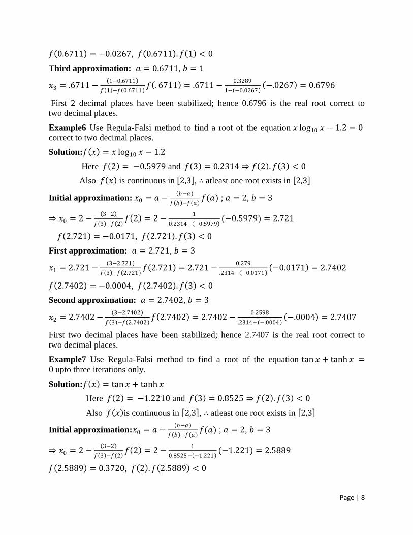
𝑓 0.6711 = −0.0267, 𝑓 0.6711 . 𝑓 1 < 0
Third approximation: 𝑎 = 0.6711, 𝑏 = 1
𝑥3 = .6711 − 1−0.6711
𝑓 1 −𝑓 0.6711 𝑓 . 6711 = .6711 −
0.3289
1− −0.0267 −.0267 = 0.6796
First 2 decimal places have been stabilized; hence 0.6796 is the real root correct to
two decimal places.
Example6 Use Regula-Falsi method to find a root of the equation 𝑥 log10 𝑥 − 1.2 = 0 correct to two decimal places.
Solution:𝑓 𝑥 = 𝑥 log10 𝑥 − 1.2
Here 𝑓 2 = −0.5979 and 𝑓 3 = 0.2314 ⇒ 𝑓 2 . 𝑓 3 < 0
Also 𝑓 𝑥 is continuous in 2,3 , ∴ atleast one root exists in 2,3
Initial approximation: 𝑥0 = 𝑎 − 𝑏−𝑎
𝑓 𝑏 −𝑓 𝑎 𝑓(𝑎) ; 𝑎 = 2, 𝑏 = 3
⇒ 𝑥0 = 2 − 3−2
𝑓 3 −𝑓 2 𝑓 2 = 2 −
1
0.2314− −0.5979 (−0.5979) = 2.721
𝑓 2.721 = −0.0171, 𝑓 2.721 . 𝑓 3 < 0
First approximation: 𝑎 = 2.721, 𝑏 = 3
𝑥1 = 2.721 − 3−2.721
𝑓 3 −𝑓 2.721 𝑓 2.721 = 2.721 −
0.279
.2314− −0.0171 −0.0171 = 2.7402
𝑓 2.7402 = −0.0004, 𝑓 2.7402 . 𝑓 3 < 0
Second approximation: 𝑎 = 2.7402, 𝑏 = 3
𝑥2 = 2.7402 − 3−2.7402
𝑓 3 −𝑓 2.7402 𝑓 2.7402 = 2.7402 −
0.2598
.2314− −.0004 −.0004 = 2.7407
First two decimal places have been stabilized; hence 2.7407 is the real root correct to
two decimal places.
Example7 Use Regula-Falsi method to find a root of the equation tan 𝑥 + tanh 𝑥 =0 upto three iterations only.
Solution:𝑓 𝑥 = tan 𝑥 + tanh 𝑥
Here 𝑓 2 = −1.2210 and 𝑓 3 = 0.8525 ⇒ 𝑓 2 . 𝑓 3 < 0
Also 𝑓 𝑥 is continuous in 2,3 , ∴ atleast one root exists in 2,3
Initial approximation:𝑥0 = 𝑎 − 𝑏−𝑎
𝑓 𝑏 −𝑓 𝑎 𝑓(𝑎) ; 𝑎 = 2, 𝑏 = 3
⇒ 𝑥0 = 2 − 3−2
𝑓 3 −𝑓 2 𝑓 2 = 2 −
1
0.8525− −1.221 (−1.221) = 2.5889
𝑓 2.5889 = 0.3720, 𝑓 2 . 𝑓 2.5889 < 0

Page | 9
First approximation: 𝑎 = 2, 𝑏 = 2.5889
𝑥1 = 2 − 2.5889−2
𝑓 2.5889 −𝑓 2 𝑓 2 = 2 −
0.5889
0.3720− −1.2210 (−1.2210) = 2.4514
𝑓 2.4514 = 0.1596, 𝑓 2 . 𝑓 2.4514 < 0
Second approximation: 𝑎 = 2, 𝑏 = 2.4514
𝑥2 = 2 − 2.4514−2
𝑓 2.4514 −𝑓 2 𝑓 2 = 2 −
0.4514
0.1596− −1.2210 (−1.2210) = 2.3992
𝑓 2.3992 = 0.0662, 𝑓 2 . 𝑓 2.3992 < 0
Third approximation: 𝑎 = 2, 𝑏 = 2.3992
𝑥2 = 2 − 2.3992−2
𝑓 2.3992 −𝑓 2 𝑓 2 = 2 −
0.3992
0.0662− −1.2210 (−1.2210) = 2.3787
∴Real root of the equationtan 𝑥 + tanh 𝑥 = 0 after three iterations is 2.3787
Example8 Use Regula-Falsi method to find a root of the equation 𝑥𝑒𝑥 − 2 = 0 correct to
three decimal places.
Solution: 𝑓 𝑥 = 𝑥𝑒𝑥 − 2
Here 𝑓 0 = −2 and 𝑓 1 = 0.7183 ⇒ 𝑓 0 . 𝑓 1 < 0
Also 𝑓 𝑥 is continuous in 0,1 , ∴ atleast one root exists in 0,1
Initial approximation: 𝑥0 = 𝑎 − 𝑏−𝑎
𝑓 𝑏 −𝑓 𝑎 𝑓(𝑎) ; 𝑎 = 0, 𝑏 = 1
⇒ 𝑥0 = 0 − 1−0
𝑓 1 −𝑓 0 𝑓 0 = 0 −
1
0.7183− −2 (−2) = 0.7358
𝑓 0.7358 = −0.4643, 𝑓 0.7358 . 𝑓 1 < 0
First approximation: 𝑎 = 0.7358, 𝑏 = 1
𝑥1 = 0.7358 − 1−0.7358
𝑓 1 −𝑓 0.7358 𝑓 0.7358 = 0.7358 −
0.2642
0.7183− −0.4643 (−0.4643) =
0.8395
𝑓 0.8395 = −0.0564, 𝑓 0.8395 . 𝑓 1 < 0
Second approximation: 𝑎 = 0.8395, 𝑏 = 1
𝑥2 = 0.8395 − 1−0.8395
𝑓 1 −𝑓 0.8395 𝑓 0.8395 = 0.8395 −
0.1605
0.7183− −0.0564 (−0.0564) =
0.8512
𝑓 0.8512 = −0.006, 𝑓 0.8512 . 𝑓 1 < 0
Third approximation: 𝑎 = 0.8512, 𝑏 = 1
𝑥2 = 0.8512 − 1−0.8512
𝑓 1 −𝑓 0.8512 𝑓 0.8512 = 0.8512 −
0.1488
0.7183− −0.006 (−0.006) = 0.8524
𝑓 0.8524 = −0.009, 𝑓 0.8524 . 𝑓 1 < 0

Page | 10
Fourth approximation: 𝑎 = 0.8474 𝑏 = 1
𝑥4 = 0.8524 − 1−0.8524
𝑓 1 −𝑓 0.8524 𝑓 0.8524 = 0.8524 −
0.1476
0.7183− −0.0009 (−0.0009) =
0.8526
𝑓 0.8526 = −0.00002~0,
∴ Real root of the equation 𝑥𝑒𝑥 − 2 = 0 correct to three decimal places is 0.8526
5.2.3 Newton-Raphson Method (Geometrical Interpretation) Newton-Raphson method named after Isaac Newton and Joseph Raphson is a powerful
technique for solving equations numerically. The Newton-Raphson method in one
variable is implemented as follows:
Let 𝛼 be an exact root and 𝑥0 be the initial approximate
root of the equation 𝑓 𝑥 = 0. First approximation 𝑥1 is
taken by drawing a tangent to curve 𝑦 = 𝑓 𝑥 at the
point 𝑥0, 𝑓 𝑥0 . If 𝜃 is the angle which tangent
through the point 𝑥0, 𝑓 𝑥0 makes with 𝑥- axis, then
slope of the tangent is given by:
tan 𝜃 = 𝑓 𝑥0
𝑥0−𝑥1= 𝑓′ 𝑥0
⇒ 𝑥1 = 𝑥0 −𝑓 𝑥0
𝑓′ 𝑥0
Similarly 𝑥2 = 𝑥1 −𝑓 𝑥1
𝑓′ 𝑥1
⋮ The required root to desired accuracy is obtained by drawing tangents to the curve
at points 𝑥𝑛 , 𝑓 𝑥𝑛 successively.
∴ 𝑥𝑛+1 = 𝑥𝑛 −𝑓 𝑥𝑛
𝑓′ 𝑥𝑛
Newton-Raphson method works very fast but sometimes it fails to converge as shown
below:
Case I:
If any of the approximations encounters a zero
derivative (extreme point), then the tangent at that
point goes parallel to 𝑥-axis, resulting in no further
approximations as shown in given figure where third
approximation tends to infinity.
Case II:
Sometimes Newton-Raphson method may run into an
infinite cycle or loop as shown in adjoining figure.
Change in initial approximation may untangle the
problem.
𝜽
𝒙𝟎,𝒇 𝒙𝟎

Page | 11
Case III:
In case of a point of discontinuity, as shown in given
figure, subsequent roots may diverge instead of
converging.
Remarks:
Newton-Raphson method can be used for solving both algebraic and
transcendental equations and it can also be used when roots are complex.
Initial approximation 𝑥0 can be taken randomly in the interval 𝑎, 𝑏 , such
that 𝑓 𝑎 . 𝑓 𝑏 < 0
Newton-Raphson method has quadratic convergence, but in case of bad choice
of 𝑥0 (the initial guess), Newton- Raphson method may fail to converge
This method is useful in case of large value of 𝑓′ 𝑥𝑛 i.e. when graph of 𝑓 𝑥
while crossing 𝑥 -axis is nearly vertical
Example 9 Use Newton-Raphson method to find a root of the equation 𝑥3 − 5𝑥 + 3 = 0 correct to three decimal places.
Solution: 𝑓 𝑥 = 𝑥3 − 5𝑥 + 3
⇒ 𝑓′ 𝑥 = 3𝑥2 − 5
Here 𝑓 0 = 3 and 𝑓 1 = −1 ⇒ 𝑓 0 . 𝑓 1 < 0
Also 𝑓 𝑥 is continuous in 0,1 , ∴ atleast one root exists in 0,1
Initial approximation: Let initial approximation 𝑥0 in the interval 0,1 be 0.8
By Newton-Raphson method 𝑥𝑛+1 = 𝑥𝑛 −𝑓 𝑥𝑛
𝑓′ 𝑥𝑛
First approximation:
𝑥1 = 𝑥0 −𝑓 𝑥0
𝑓′ 𝑥0 , where 𝑥0 = 0.8, 𝑓 0.8 = −0.488, 𝑓′ 0.8 = −3.08
⇒ 𝑥1 = 0.8 −−0.488
−3.08= 0.6416
Second approximation:
𝑥2 = 𝑥1 −𝑓 𝑥1
𝑓′ 𝑥1 , where 𝑥1 = 0.6415 , 𝑓 0.6416 = 0.0561 , 𝑓′ 0.6416 = −3.7650
⇒ 𝑥2 = 0.6416 −0.05611
−3.7650= 0.6565
Third approximation:
𝑥3 = 𝑥2 −𝑓 𝑥2
𝑓′ 𝑥2 , where 𝑥2 = 0.6565 , 𝑓 0.6565 = 0.0004 , 𝑓′ 0.6565 = −3.7070
⇒ 𝑥3 = 0.6565 −0.0004
−3.7070= 0.6566
Hence a root of the equation 𝑥3 − 5𝑥 + 3 = 0 correct to three decimal places is 0.6566
Page | 12
Example 10 Find the approximate value of 28 correct to 3 decimal places using
Newton Raphson method.
Solution: 𝑥 = 28 ⇒ 𝑥2 − 28 = 0
∴ 𝑓 𝑥 = 𝑥2 − 28
⇒ 𝑓′ 𝑥 = 2𝑥
Here 𝑓 5 = −3 and 𝑓 6 = 8 ⇒ 𝑓 5 . 𝑓 6 < 0
Also 𝑓 𝑥 is continuous in 5,6 , ∴ atleast one root exists in 5,6
Initial approximation: Let initial approximation 𝑥0 in the interval 5,6 be 5.5
By Newton-Raphson method 𝑥𝑛+1 = 𝑥𝑛 −𝑓 𝑥𝑛
𝑓′ 𝑥𝑛
First approximation:
𝑥1 = 𝑥0 −𝑓 𝑥0
𝑓′ 𝑥0 , where 𝑥0 = 5.5, 𝑓 5.5 = 2.25, 𝑓′ 5.5 = 11
⇒ 𝑥1 = 5.5 −𝟐.𝟐𝟓
11= 5.2955
Second approximation:
𝑥2 = 𝑥1 −𝑓 𝑥1
𝑓′ 𝑥1 , where 𝑥1 = 5.2955, 𝑓 5.2955 = 0.0423, 𝑓′ 5.2955 = 10.591
⇒ 𝑥2 = 5.2955 −0.0423
10.591= 5.2915
Third approximation:
𝑥3 = 𝑥2 −𝑓 𝑥2
𝑓′ 𝑥2 , where 𝑥2 = 5.2915, 𝑓 5.2915 = −0.00003, 𝑓′ 5.2915 = 10.583
⇒ 𝑥3 = 5.2915 −−0.00003
10.583= 5.2915
Hence value of 28 correct to three decimal places is 5.2915
Example 11 Use Newton-Raphson method to find a root of the equation 𝑥 sin 𝑥 +cos 𝑥 = 0 correct to three decimal places.
Solution: 𝑓 𝑥 = 𝑥 sin 𝑥 + cos 𝑥
⇒ 𝑓′ 𝑥 = 𝑥 cos 𝑥 + sin 𝑥 − sin 𝑥 = 𝑥 cos 𝑥
Here 𝑓 𝜋
2 = 1.5708 and 𝑓 𝜋 = −1 ⇒ 𝑓
𝜋
2 . 𝑓 𝜋 < 0
Also 𝑓 𝑥 is continuous in 𝜋
2, 𝜋 ∴ atleast one root exists in
𝜋
2, 𝜋
Initial approximation: Let initial approximation 𝑥0 in the interval 𝜋
2, 𝜋 be 𝜋

Page | 13
By Newton-Raphson method 𝑥𝑛+1 = 𝑥𝑛 −𝑓 𝑥𝑛
𝑓′ 𝑥𝑛
First approximation:
𝑥1 = 𝑥0 −𝑓 𝑥0
𝑓′ 𝑥0 , where 𝑥0 = 𝜋, 𝑓 𝜋 = −1, 𝑓′ 𝜋 = −3.1416
⇒ 𝑥1 = 3.1416 −−1
−3.1416= 2.8233
Second approximation:
𝑥2 = 𝑥1 −𝑓 𝑥1
𝑓′ 𝑥1 , where 𝑥1 = 2.8233, 𝑓 2.8233 = −0.0662, 𝑓′ 2.8233 = −2.6815
⇒ 𝑥2 = 2.8233 −−0.0662
−2.6815= 2.7986
Third approximation:
𝑥3 = 𝑥2 −𝑓 𝑥2
𝑓′ 𝑥2 , where 𝑥2 = 2.798, 𝑓 2.7986 = −0.0006, 𝑓′ 2.7986 = −2.6356
⇒ 𝑥3 = 2.7986 −−0.0006
−2.6356= 2.7984
Hence a root of the equation 𝑥 sin 𝑥 + cos 𝑥 = 0 correct to three decimal places is
2.7984
Example 12 Use Newton Raphson method to derive a formula to find 𝑁5
, 𝑁𝜖𝑅.
Hence evaluate 435
correct to 3 decimal places.
Solution: 𝑥 = 𝑁5
⇒ 𝑥5 − 𝑁 = 0
𝑓 𝑥 = 𝑥5 − 𝑁
⇒ 𝑓′ 𝑥 = 5𝑥4
By Newton-Raphson method 𝑥𝑛+1 = 𝑥𝑛 −𝑓 𝑥𝑛
𝑓′ 𝑥𝑛
⇒ 𝑥𝑛+1 = 𝑥𝑛 −𝑥𝑛
5−𝑁
5𝑥𝑛4 =
4
5𝑥𝑛 +
𝑁
5𝑥𝑛4
To evaluate 435
, putting 𝑁 = 43 , ∴Newton-Raphson formula is given by
𝑥𝑛+1 =4
5𝑥𝑛 +
43
5𝑥𝑛4
Let initial approximation 𝑥0 be 2
First approximation:
𝑥1 =4
5𝑥0 +
43
5𝑥04 , where 𝑥0 = 2
⇒ 𝑥1 =8
5+
43
80= 2.1375

Page | 14
Second approximation:
𝑥2 =4
5𝑥1 +
43
5𝑥14 , where 𝑥1 = 2.1375
⇒ 𝑥2 =4(2.1375)
5+
43
5(2.1375)4= 2.1220
Third approximation:
𝑥3 =4
5𝑥2 +
43
5𝑥24 , where 𝑥2 = 2.1220
⇒ 𝑥3 =4(2.1220)
5+
43
5(2.1220)4= 2.1217
Fourth approximation:
𝑥4 =4
5𝑥3 +
43
5𝑥34 , where 𝑥3 = 2.1217
⇒ 𝑥4 =4(2.1217)
5+
43
5(2.1217)4= 2.1217
Hence value of 435
correct to four decimal places is 2.1217
5.2.3.1 Generalized Newton’s Method for Multiple Roots
Result: If 𝛼 is a root of equation 𝑓 𝑥 = 0 with multiplicity 𝑚, then it is also a root of
equation 𝑓′ 𝑥 = 0 with multiplicity (𝑚 − 1) and also of the equation 𝑓′′ 𝑥 = 0 with
multiplicity (𝑚 − 1) and so on.
For example (𝑥 − 1)3 = 0 has ‘1’ as a root with multiplicity 3
3(𝑥 − 1)2 = 0 has ‘1’ as the root with multiplicity 2
6(𝑥 − 1) = 0 has ‘1’ as the root with multiplicity 1
∴ The expressions 𝑥𝑛 − 𝑚𝑓 𝑥𝑛
𝑓′ 𝑥𝑛 , 𝑥𝑛 − (𝑚 − 1)
𝑓′ 𝑥𝑛
𝑓′′ 𝑥𝑛 , 𝑥𝑛 − (𝑚 − 2)
𝑓′′ 𝑥𝑛
𝑓′′′ 𝑥𝑛 are
equivalent
Generalized Newton’s method is used to find repeated roots of an equation as is given as:
If 𝛼 be a root of equation 𝑓 𝑥 = 0 which is repeated 𝑚 times,
Then 𝑥𝑛+1 = 𝑥𝑛 − 𝑚𝑓 𝑥𝑛
𝑓′ 𝑥𝑛 ~ 𝑥𝑛 − (𝑚 − 1)
𝑓′ 𝑥𝑛
𝑓′′ 𝑥𝑛
Example 13 Use Newton-Raphson method to find a double root of the equation
𝑥3 − 𝑥2 − 𝑥 + 1 = 0 upto three iterations.
Solution: 𝑓 𝑥 = 𝑥3 − 𝑥2 − 𝑥 + 1
𝑓′ 𝑥 = 3𝑥2 − 2𝑥 − 1
𝑓 ′′ (𝑥) = 6𝑥 − 2

Page | 15
Let the initial approximation 𝑥0 = 0.7
First approximation:
𝑥1 = 𝑥0 −2𝑓 𝑥0
𝑓′ 𝑥0 Also 𝑥1 = 𝑥0 −
𝑓′ 𝑥0
𝑓′′ 𝑥0
⇒ 𝑥1 = 0.7 −0.306
−0.93= 1.0290 And 𝑥1 = 0.7 −
−0.93
2.2= 1.1227
∴ 𝑥1 =1.029+1.1227
2= 1.0759, 𝑓(𝑥1) = .012
Second approximation:
𝑥2 = 𝑥1 −2𝑓 𝑥1
𝑓′ 𝑥1 Also 𝑥2 = 𝑥1 −
𝑓′ 𝑥1
𝑓′′ 𝑥1
⇒ 𝑥2 = 1.0759 −0.0239
0.3209= 1.001 And 𝑥2 = 1.0759 −
0.3209
4.4554= 1.004
∴ 𝑥2 =1.001+1.004
2= 1.0025 , 𝑓(𝑥2) = .00001
Third approximation:
𝑥3 = 𝑥2 −2𝑓 𝑥2
𝑓′ 𝑥2 Also 𝑥3 = 𝑥2 −
𝑓′ 𝑥2
𝑓′′ 𝑥2
⇒ 𝑥3 = 1.0025 −0.00003
0.0100= 0.995 And 𝑥3 = 1.0025 −
0.0100
4.015= 1.0000
∴ 𝑥3 =0.995+1.000
2= 0.9975 , 𝑓(𝑥3) = .00001
The double root of the equation 𝑥3 − 𝑥2 − 𝑥 + 1 = 0 after three iterations is
0.9975.
5.2.3.1 Convergence of Newton Raphson Method
Let 𝛼 be an exact root of the equation 𝑓 𝑥 = 0
⇒ 𝑓 𝛼 = 0
Also let 𝑥𝑛 and 𝑥𝑛+1 be two successive approximations to the root 𝛼.
If ∈𝑛 and ∈𝑛+1 are the corresponding errors in the approximations 𝑥𝑛 and 𝑥𝑛+1
Then 𝑥𝑛 = 𝛼 +∈𝑛 … ①
and 𝑥𝑛+1 = 𝛼 +∈𝑛+1 … ②
Now by Newton Raphson method
𝑥𝑛+1 = 𝑥𝑛 −𝑓 𝑥𝑛
𝑓′ 𝑥𝑛 … ③
Using ① and ② in ③
⇒ 𝛼 +∈𝑛+1= 𝛼 +∈𝑛−𝑓 𝛼+∈𝑛
𝑓′ 𝛼+∈𝑛

Page | 16
⇒∈𝑛+1=∈𝑛𝑓 ′ 𝛼+∈𝑛 −𝑓(𝛼+∈𝑛 )
𝑓 ′ (𝛼+∈𝑛 )
⇒∈𝑛+1=∈𝑛 𝑓 ′ 𝛼 +∈𝑛𝑓 ′′ 𝛼 + … − 𝑓 𝛼 +∈𝑛𝑓 ′ 𝛼 +
∈𝑛2
2!𝑓 ′′ 𝛼 +⋯
𝑓 ′ 𝛼 +∈𝑛𝑓 ′′ 𝛼 + … By Taylor’s expansion
⇒∈𝑛+1=∈𝑛
2𝑓 ′′ 𝛼 − ∈𝑛
2
2!𝑓 ′′ 𝛼 +⋯
𝑓 ′ 𝛼 1+∈𝑛𝑓′′ 𝛼
𝑓′ 𝛼 +⋯
∵ 𝑓 𝛼 = 0
⇒∈𝑛+1= ∈𝑛
2
2
𝑓 ′′ (𝛼)
𝑓 ′ (𝛼)+ ⋯ 1 +
∈𝑛𝑓 ′′ 𝛼
𝑓 ′ 𝛼 + ⋯
−1
⇒∈𝑛+1= ∈𝑛
2
2
𝑓 ′′ (𝛼)
𝑓 ′ (𝛼)+ ⋯ 1 −
∈𝑛𝑓 ′′ 𝛼
𝑓 ′ 𝛼 + ⋯
⇒∈𝑛+1=∈𝑛
2
2
𝑓 ′′ (𝛼)
𝑓 ′ (𝛼) Neglecting higher order terms
⇒∈𝑛+1= 𝐾 ∈𝑛2 Where 𝑘 =
1
2
𝑓 ′′ (𝛼)
𝑓 ′ (𝛼)
∴ Newton Raphson method has convergence of order 2 or quadratic convergence.
5.3 Iterative Methods for Solving Simultaneous Linear Equations
Consider a system of linear equations:
𝑎1𝑥 + 𝑏1𝑦 + 𝑐1𝑧 = 𝑑1
𝑎2𝑥 + 𝑏2𝑦 + 𝑐2𝑧 = 𝑑2
𝑎3𝑥 + 𝑏3𝑦 + 𝑐3𝑧 = 𝑑3
…①
We have been using direct methods for solving a system of linear equations. Direct
methods produce exact solution after a finite number of steps whereas iterative
methods give a sequence of approximate solutions until solution is obtained up to
desired accuracy. Common iterative methods for solving a system of linear
equations are:
1. Gauss-Jacobi’s iteration method
2. Gauss-Seidal’s iteration method
These methods require partial pivoting before application.
Partial pivoting: It is about changing rows of a system of linear equations given by
① such that 𝑎1 ≥ 𝑎2 , 𝑎3 ; 𝑏2 ≥ 𝑏3.
Complete pivoting: It is the process of selecting the largest element in the magnitude
as the pivot element by interchanging row as well as columns of the system. Order
of variables is also changed in the procedure. In particular for the system given by ①,
complete pivoting would require 𝑎1 ≥ 𝑎2, 𝑎3 ; 𝑏2 ≥ 𝑏1, 𝑏3 , if 𝑎1 and 𝑏2 are to be
taken as pivots.

Page | 17
5.3.1 Gauss-Jacobi’s Iteration Method
The concept of the Gauss- Jacobi’s iteration scheme is extremely simple with the
assumptions that the system has unique solution and diagonal elements are non-zeros.
Algorithm: Gauss-Jacobi’s iteration method
1. Take the system of linear equations given by ① after partial pivoting and solve
each equation in the system for the diagonal value of variables such that
𝑥 =1
𝑎1(𝑑1 − 𝑏1𝑦 − 𝑐1𝑧)
𝑦 =1
𝑏2(𝑑2 − 𝑎2𝑥 − 𝑐2𝑧)
𝑧 =1
𝑐3(𝑑3 − 𝑎3𝑥 − 𝑏3𝑦)
…②
2. Rewrite ② in generalized form given by:
𝑥𝑛+1 =1
𝑎1(𝑑1 − 𝑏1𝑦𝑛 − 𝑐1𝑧𝑛)
𝑦𝑛+1 =1
𝑏2(𝑑2 − 𝑎2𝑥𝑛 − 𝑐2𝑧𝑛)
𝑧𝑛+1 =1
𝑐3(𝑑3 − 𝑎3𝑥𝑛 − 𝑏3𝑦𝑛 )
…③
3. Take 𝑥0 = 𝑦0 = 𝑧0 = 0 as initial approximation (in general if a better
approximation can not be judged) and substitute in the system given by ③
∴ 𝑥1 =𝑑1
𝑎1 , 𝑦1 =
𝑑2
𝑏2 , 𝑧1 =
𝑑3
𝑐3
4. Putting 𝑛 = 1 , substitute the values of 𝑥1 , 𝑦1 and 𝑧1 in ③ to get next
approximations of 𝑥2, 𝑦2 and 𝑧2. Continue the procedure until the difference
between two consecutive approximations is negligible.
Example 14 Solve the following system of equations using Gauss Jacobi's method
5𝑥 − 2𝑦 + 3𝑧 = −1
−3𝑥 + 9𝑦 + 𝑧 = 2
2𝑥 − 𝑦 − 7𝑧 = 3
Solution: The given system of equations is satisfying rules of partial pivoting.
Rewriting in general form as given in ③
𝑥𝑛+1 =1
5(−1 + 2𝑦𝑛 − 3𝑧𝑛)
𝑦𝑛+1 =1
9 2 + 3𝑥𝑛 − 𝑧𝑛
𝑧𝑛+1 =1
7 −3 + 2𝑥𝑛 − 𝑦𝑛
Taking 𝑥0 = 𝑦0 = 𝑧0 = 0 as initial approximation
First Approximation:
𝑥1 = −1
5= −0.2 𝑦1 =
2
9= 0.222 , 𝑧1 = −
3
7= −0.429

Page | 18
Second Approximation:
𝑥2 =1
5 −1 + 2𝑦1 − 3𝑧1 , 𝑦2 =
1
9 2 + 3𝑥1 − 𝑧1 , 𝑧2 =
1
7(−3 + 2𝑥1 − 𝑦1)
⇒ 𝑥2 =1
5 −1 + 2 0.222 − 3(−0.429 ) = 0.146
𝑦2 =1
9 2 + 3(−0.2 + 0.429) = 0.203
𝑧2 =1
7 −3 + 2 −0.2 − 0.222 = −0.517
Third Approximation:
𝑥3 =1
5 −1 + 2𝑦2 − 3𝑧2 , 𝑦3 =
1
9 2 + 3𝑥2 − 𝑧2 , 𝑧3 =
1
7(−3 + 2𝑥2 − 𝑦2)
⇒ 𝑥3 =1
5 −1 + 2 0.203 − 3(−0.517 ) = 0.191
𝑦3 =1
9 2 + 3(0.146 + 0.517) = 0.328
𝑧3 =1
7 −3 + 2 0.146 − 0.203 = −0.416
Fourth Approximation:
𝑥4 =1
5 −1 + 2𝑦3 − 3𝑧3 , 𝑦4 =
1
9 2 + 3𝑥3 − 𝑧3 , 𝑧4 =
1
7(−3 + 2𝑥3 − 𝑦3)
⇒ 𝑥4 =1
5 −1 + 2 0.328 − 3(−0.416 ) = 0.181
𝑦4 =1
9 2 + 3(0.191 + 0.416) = 0.332
𝑧4 =1
7 −3 + 2 0.191 − 0.328 = −0.421
Fifth Approximation:
𝑥5 =1
5 −1 + 2𝑦4 − 3𝑧4 , 𝑦5 =
1
9 2 + 3𝑥4 − 𝑧4 , 𝑧5 =
1
7(−3 + 2𝑥4 − 𝑦4)
⇒ 𝑥5 =1
5 −1 + 2 0.332 − 3(−0.421 ) = 0.185
𝑦5 =1
9 2 + 3(0.181 + 0.421) = 0.329
𝑧5 =1
7 −3 + 2 0.181 − 0.332 = −0.424
Sixth Approximation:
𝑥6 =1
5 −1 + 2𝑦5 − 3𝑧5 , 𝑦6 =
1
9 2 + 3𝑥5 − 𝑧5 , 𝑧6 =
1
7(−3 + 2𝑥5 − 𝑦5)
⇒ 𝑥6 =1
5 −1 + 2 0.329 − 3(−0.424 ) = 0.186
𝑦6 =1
9 2 + 3(0.185 + 0.424) = 0.331
𝑧6 =1
7 −3 + 2 0.185 − 0.329 = −0.423

Page | 19
Values of variables have been stabilized, ∴ approximate solution is given by
𝑥 = 0.186, 𝑦 = 0.331and 𝑧 = −0.423
Example 15 Compute 4 iterations to find an approximate solution of the given system of
equations using Gauss Jacobi's method.
𝑥 + 𝑦 + 5𝑧 = −1
5𝑥 − 𝑦 + 𝑧 = 10
2𝑥 + 4𝑦 = 12
Solution: Rearranging the given equations by partial pivoting
5𝑥 − 𝑦 + 𝑧 = 10
2𝑥 + 4𝑦 = 12
𝑥 + 𝑦 + 5𝑧 = −1
Rewriting in general form as given in ③
𝑥𝑛+1 =1
5(10 + 𝑦𝑛 − 𝑧𝑛 )
𝑦𝑛+1 =1
4 12 − 2𝑥𝑛
𝑧𝑛+1 =1
5(−1 − 𝑥𝑛 − 𝑦𝑛)
Taking 𝑥0 = 𝑦0 = 𝑧0 = 0 as initial approximation
First Approximation:
𝑥1 =10
5= 2 , 𝑦1 =
12
4= 3 , 𝑧1 = −
1
5
Second Approximation:
𝑥2 =1
5 10 + 𝑦1 − 𝑧1 , 𝑦2 =
1
4 12 − 2𝑥1 , 𝑧2 =
1
5(−1 − 𝑥1 − 𝑦1)
⇒ 𝑥2 =1
5 10 + 3 +
1
5 , 𝑦2 =
1
4 12 − 4 , 𝑧2 =
1
5(−1 − 2 − 3)
∴ 𝑥2 = 2.64 , 𝑦2 = 2 , 𝑧2 = −1.2
Third Approximation:
𝑥3 =1
5 10 + 𝑦2 − 𝑧2 , 𝑦3 =
1
4 12 − 2𝑥2 , 𝑧3 =
1
5(−1 − 𝑥2 − 𝑦2)
⇒ 𝑥3 =1
5 10 + 2 + 1.2 , 𝑦3 =
1
4 12 − 2(2.64) , 𝑧3 =
1
5(−1 − 2.64 − 2)
∴ 𝑥3 = 2.64 , 𝑦3 = 1.68 , 𝑧3 = −0.928
Fourth Approximation:
𝑥4 =1
5 10 + 𝑦3 − 𝑧3 , 𝑦3 =
1
4 12 − 2𝑥3 , 𝑧3 =
1
5(−1 − 𝑥3 − 𝑦3)
⇒ 𝑥4 =1
5 10 + 1.68 + 0.928 , 𝑦4 =
1
4 12 − 2(2.64) , 𝑧4 =
1
5(−1 − 2.64 − 1.68)

Page | 20
∴ 𝑥4 = 2.52 , 𝑦4 = 1.68 , 𝑧4 = −1.064
Approximate solution after 4 iterations is given by 𝑥 = 2.52, 𝑦 = 1.68, 𝑧 = −1.064
5.3.2Gauss-Seidal’s Iteration Method
Gauss-Seidel method is an improvement of the basic Gauss-Jordan method. Here the
improved values of variables are utilized as soon as they are obtained.
∴ System of equations given in ③ is improved by taking latest values of the variables
as
𝑥𝑛+1 =1
𝑎1 𝑑1 − 𝑏1𝑦𝑛 − 𝑐1𝑧𝑛
𝑦𝑛+1 =1
𝑏2 𝑑2 − 𝑎2𝑥𝑛+1 − 𝑐2𝑧𝑛
𝑧𝑛+1 =1
𝑐3 𝑑3 − 𝑎3𝑥𝑛+1 − 𝑏3𝑦𝑛+1
Gauss-Seidel scheme usually converges faster than Jacobi’s iteration method.
Example 16 Solve the system of equations given in Example 14 using Gauss Seidal's
method
5𝑥 − 2𝑦 + 3𝑧 = −1
−3𝑥 + 9𝑦 + 𝑧 = 2
2𝑥 − 𝑦 − 7𝑧 = 3
Also compare the results obtained in two methods.
Solution: The given system of equations is satisfying rules of partial pivoting.
Using Gauss Seidal's approximations, system can be rewritten as
𝑥𝑛+1 =1
5 −1 + 2𝑦𝑛 − 3𝑧𝑛
𝑦𝑛+1 =1
9 2 + 3𝑥𝑛+1 − 𝑧𝑛
𝑧𝑛+1 =1
7 −3 + 2𝑥𝑛+1 − 𝑦𝑛+1
Taking 𝑥0 = 𝑦0 = 𝑧0 = 0 as initial approximation
First Approximation:
𝑥1 = −1
5= −0.2 𝑦1 =
2
9= 0.222 , 𝑧1 = −
3
7= −0.429
Second Approximation:
𝑥2 =1
5 −1 + 2𝑦1 − 3𝑧1 , 𝑦2 =
1
9 2 + 3𝑥2 − 𝑧1 , 𝑧2 =
1
7(−3 + 2𝑥2 − 𝑦2)
⇒ 𝑥2 =1
5 −1 + 2 0.222 − 3(−0.429 ) = 0.146
𝑦2 =1
9 2 + 3(0.146 + 0.429) = 0.319

Page | 21
𝑧2 =1
7 −3 + 2 0.146 − 0.319 = −0.432
Third Approximation:
𝑥3 =1
5 −1 + 2𝑦2 − 3𝑧2 , 𝑦3 =
1
9 2 + 3𝑥3 − 𝑧2 , 𝑧3 =
1
7(−3 + 2𝑥3 − 𝑦3)
⇒ 𝑥3 =1
5 −1 + 2 0.319 − 3(−0.432 ) = 0.187
𝑦3 =1
9 2 + 3(0.187 + 0.432) = 0.333
𝑧3 =1
7 −3 + 2 0.187 − 0.333 = −0.423
Fourth Approximation:
𝑥4 =1
5 −1 + 2𝑦3 − 3𝑧3 , 𝑦4 =
1
9 2 + 3𝑥4 − 𝑧3 , 𝑧4 =
1
7(−3 + 2𝑥4 − 𝑦4)
⇒ 𝑥4 =1
5 −1 + 2 0.333 − 3(−0.423 ) = 0.187
𝑦4 =1
9 2 + 3(0.187 + 0.423) = 0.332
𝑧4 =1
7 −3 + 2 0.187 − 0.332 = −0.423
Values of variables have been stabilized, ∴ approximate solution is given by
𝑥 = 0.187, 𝑦 = 0.332 and 𝑧 = −0.423
Clearly numbers of iterations for the solution to converge in Gauss Seidal’s
method are much less than Gauss Jacobi’s method.
Exercise 5A
1. Find the real root of the equation 𝑥3 − 2𝑥 − 5 = 0 correct to three decimal
places using Bisection method.
2. Perform three iterations to find root of the equation 𝑥𝑒𝑥 − cos 𝑥 = 0 using
Regula-Falsi method.
3. Find the real root of the equation 𝑥3 − 3𝑥 − 5 = 0 correct to three decimal
places using Newton- Raphson method.
4. Solve the system of equations:
10𝑥1 − 2𝑥2 − 𝑥3 − 𝑥4 = 3
2𝑥1 − 10𝑥2 + 𝑥3 + 𝑥4 = −15
𝑥1 + 𝑥2 − 10𝑥3 + 2𝑥4 = −27
𝑥1 + 𝑥2 + 2𝑥3 − 10𝑥4 = 9 using Gauss- Jacobi method. Compute results for 2 iterations.
5. Solve the system of equations given in Q4 upto 2 iterations, using Gauss-
Seidal method.

Page | 22
Answers
1. 2.0944
2. 0.494015
3. 2.279
4. 𝑥1 = 0.78, 𝑥2 = 1.74, 𝑥3 = 2.7, 𝑥4 = −0.18 taking initial
approximations as zero.
5. 𝑥1 = 0.8869, 𝑥2 = 1.9523, 𝑥3 = 2.9566, 𝑥4 = −0.0248 taking
initial approximations as zero.