Embed Size (px)
Citation preview
NUMERICAL STUDY OF ABUTMENT SCOUR IN COHESIVE SOILS
A Dissertation
by
XINGNIAN CHEN
Submitted to the Office of Graduate Studies of Texas A&M University
in partial fulfillment of the requirements for the degree of
DOCTOR OF PHILOSOPHY
December 2008
Major Subject: Civil Engineering

NUMERICAL STUDY OF ABUTMENT SCOUR IN COHESIVE SOILS
A Dissertation
by
XINGNIAN CHEN
Submitted to the Office of Graduate Studies of Texas A&M University
in partial fulfillment of the requirements for the degree of
DOCTOR OF PHILOSOPHY
Approved by:
Co-Chairs of Committee, Jean-Louis Briaud Hamn-Ching Chen Committee Members, Kuang-An Chang William R. Bryant Head of Department, David V. Rosowsky
December 2008
Major Subject: Civil Engineering

iii
ABSTRACT
Numerical Study of Abutment Scour in Cohesive Soils.
(December 2008)
Xingnian Chen, B.En., Tongji University, China;
M.En., Tongji University, China
Co-Chairs of Advisory Committee: Dr. Jean-Louis Briaud Dr. Hamn-Ching Chen
This research is part of the extension of the SRICOS-EFA method for predicting
the maximum scour depth history around the bridge abutment. The basic objective is to
establish the equation for predicting the maximum bed shear stress around the abutment
at the initial condition of scouring. CHEN3D (Computerized Hydraulic ENgineering
program for 3D flow) program is utilized to perform numerical simulations and predict
bed shear stress before scouring. The Chimera technique incorporated in CHEN3D
makes the program capable of simulating all kinds of complex geometry and moving
boundary. CHEN3D program has been proven to be an accurate method to predict flow
field and boundary shear stress in many fields and used in bridge scour study in cohesive
soils for more than ten years.
The maximum bed shear stress around abutment in open rectangular channel is
studied numerically and the equation is proposed. Reynolds number is the dominant
parameter, and the parametric studies have been performed based on the dimensional
analysis. The influence of channel contraction ratio, abutment aspect ratio, water depth,
abutment shape, and skew angle has been investigated, and the corresponding correction

iv
factors have been proposed. The study of the compound channel configuration is
conducted further to extend the application of the proposed equation.
Numerical simulations of overtopping flow in straight rectangular channel, straight
compound channel and channel bend have been conducted. The bridge deck is found to
be able to change the flow distribution and the bed shear stress will increase significantly
once overtopping. The influence of the channel bend curvature, abutment location in the
channel bend, and the abutment shape is also investigated. The corresponding variation
of the bed shear stress has been concluded.
The scour models, including the erosion rate function, roughness effect, and the
turbulence kinetic energy, have been proposed and incorporated into the CHEN3D
program. One flume test case in NCHRP 24-15(2) has been simulated to determine the
parameters for the roughness and the turbulence kinetic energy. The prediction of the
maximum scour depth history with the proposed model is in good agreement with the
measurement for most cases. The influence of overtopping flow on the abutment scour
development is also studied and the corresponding correction factor is proposed.

v
ACKNOWLEDGMENTS
I would like to express my heartfelt gratitude to my co-chair, Dr. Jean-Louis
Briaud, for giving me the opportunity to study at Texas A&M University. Dr. Briaud can
always look deep into the situation to lead the best direction of the research. He is
always ready to help and encourage me.
I would like to express my special gratitude to my co-chair, Dr. Hamn-Ching
Chen for his time, effort and guidance. Dr. Chen took me into the world of
computational fluid dynamics. It is my honor to have the opportunity to work with him.
I also would like to thank Dr. Kuang-An Zhang for his valuable discussion and
guidance during the entire period of study at Texas A&M University. I wish to thank Dr.
William R. Bryant for his constant support during my Ph.D. program.
I wish to express my particular appreciation to my fellow students Sueng Jae Oh,
Po-Hung Yeh, Chao-Ming Chi, Wei Wang, and Jun Wang for their friendship and help
during different phases of this research. I would like to especially thank Sueng Jae Oh
for providing valuable experimental data.
This work is supported by NCHRP-Project 24-15(2) where Mr. David Reynaud
is the contact person.
Finally, my appreciation goes to my wife, Yufen Shao, and my parents, for their
encouragement and support during my study at Texas A&M University.
.

vi
TABLE OF CONTENTS
Page
ABSTRACT ..................................................................................................................... iii
ACKNOWLEDGMENTS .................................................................................................. v
TABLE OF CONTENTS ..................................................................................................vi
LIST OF FIGURES ........................................................................................................ viii
LIST OF TABLES ..........................................................................................................xiv
CHAPTER
I INTRODUCTION ........................................................................................................ 1
1.1 Background ........................................................................................................... 1 1.2 Objectives ............................................................................................................. 2 1.3 Methodology ......................................................................................................... 3 1.4 Dissertation Outline .............................................................................................. 6
II LITERATURE REVIEW OF BRIDGE SCOUR ........................................................ 9
2.1 Fundamentals of Bridge Scour ............................................................................. 9 2.2 Bed Shear Stress at the Bridge Crossing ............................................................ 11 2.3 Issues in the Numerical Simulation of Bridge Scour on Cohesive Soils ............ 21
III GOVERNING EQUATIONS FOR CHEN3D PROGRAM ...................................... 30
3.1 Governing Equations for Hydrodynamics .......................................................... 30 3.2 Boundary Conditions .......................................................................................... 39 3.3 Clear Water Scour ............................................................................................... 41 3.4 Overall Solution Algorithm ................................................................................ 42
IV MAXIMUM BED SHEAR STRESS AROUND ABUTMENT IN OPEN CHANNEL FLOW .................................................................................................... 44
4.1 Methodology ....................................................................................................... 44 4.2 Reference Case ................................................................................................... 48 4.3 Parametric Studies .............................................................................................. 56

vii
CHAPTER Page
4.4 Maximum Bed Shear Stress Equation in Rectangular Channel ......................... 81 4.5 Influence of the Compound Channel Congfiguration......................................... 82 4.6 Maximum Bed Shear Stress Equation in Compound Channel ........................... 91 4.7 Verification of the Maximum Bed Shear Stress Equation .................................. 92 4.8 Real Maximum Bed Shear Stress around Abutment in SRICOS Method .......... 96
V MAXIMUM BED SHEAR STRESS AROUND ABUTMENT IN OVERTOPP ING FLOW ......................................................................................... 102
5.1 Verification of the Overtopping Flow Simulation ............................................ 102 5.2 Overtopping in Rectangular Channel ............................................................... 105 5.3 Overtopping in Compound Channel ................................................................. 112 5.4 Open Channel Flow on Channel Bend ............................................................. 121 5.5 Overtopping Flow on Channel Bend ................................................................ 136 5.6 Confluence of Tributary Upstream of a Bridge ................................................ 147
VI ABUTMENT SCOUR IN COHESIVE SOILS ....................................................... 150
6.1 Soils Properties ................................................................................................. 150 6.2 Scour Model in Cohesive Soils ......................................................................... 152 6.3 Scour Prediction of the Flume Tests in NCHRP 24-15(2) ............................... 155 6.4 Scour Prediciton with Overtopping .................................................................. 179
VII CONCLUSIONS AND RECOMMENDATIONS .................................................. 187
7.1 Conclusions ....................................................................................................... 187 7.2 Recommendations ............................................................................................. 190
REFERENCES ............................................................................................................... 192
VITA .............................................................................................................................. 199
viii
LIST OF FIGURES
FIGURE Page
3-1 Finite analytic local element. .................................................................................. 37
4-1 Definition of the parameters in abutment scour problem ........................................ 45
4-2 Diagram of the reference case ................................................................................. 49
4-3 Numerical grid for the reference case ..................................................................... 51
4-4 Velocity vectors on water surface (reference case) ................................................. 52
4-5 Normalized pressure contour around vertical wall abutment .................................. 54
4-6 Bed friction coefficient (×10-2) contour for Reynolds number 105 ......................... 54
4-7 Projected velocity vectors on the cross sections around abutment ......................... 55
4-8 Normalized maximum bed shear stress versus Reynolds number .......................... 58
4-9 Bed friction coefficient (×10-2) contour for Reynolds number 104 ......................... 59
4-10 Bed friction coefficient (×10-2) contour for Reynolds number 106 ......................... 59
4-11 Bed friction coefficient (×10-2) contour for Reynolds number 107 ......................... 60
4-12 Correction factor for water depth ............................................................................ 61
4-13 Bed friction coefficient (×10-2) contour for y/Wa=0.25 ........................................... 62
4-14 Bed friction coefficient (×10-2) contour for y/Wa=0.5 ............................................. 62
4-15 Bed friction coefficient (×10-2) contour for y/Wa=1.0 ............................................. 63
4-16 Geometries for channel contraction ratio study ...................................................... 64
4-17 Correction factor for channel contraction ratio ....................................................... 65
4-18 Bed friction coefficient (×10-2) contour for rC =0.4 ............................................... 65
ix
FIGURE Page
4-19 Bed friction coefficient (×10-2) contour for rC =0.6 ............................................... 66
4-20 Bed friction coefficient (×10-2) contour for rC =0.8 ............................................... 66
4-21 Geometries for the study of abutment aspect ratio .................................................. 68
4-22 Correction factor for abutment aspect ratio ............................................................. 69
4-23 Bed friction coefficient (×10-2) contour for aL =1.2ft ............................................. 69
4-24 Bed friction coefficient (×10-2) contour for aL =2.4ft ............................................. 70
4-25 Bed friction coefficient (×10-2) contour for aL =3.33ft ........................................... 70
4-26 Bed friction coefficient (×10-2) contour for aL =4.33ft ........................................... 71
4-27 Bed friction coefficient (×10-2) contour for aL =3.33ft (WW abutment) ................ 72
4-28 Bed friction coefficient (×10-2) contour for aL =4.33ft (WW abutment) ................ 73
4-29 Bed friction coefficient (×10-2) contour for aL =5.33ft (WW abutment) ................ 73
4-30 Bed friction coefficient (×10-2) contour for aL =7.33ft (WW abutment) ................ 74
4-31 Bed friction coefficient (×10-2) contour for aL =3.33ft (ST abutment) ................... 75
4-32 Bed friction coefficient (×10-2) contour for aL =4.33ft (ST abutment) ................... 76
4-33 Bed friction coefficient (×10-2) contour for aL =5.33ft (ST abutment) ................... 76
4-34 Bed friction coefficient (×10-2) contour for aL =7.33ft (ST abutment) ................... 77
4-35 Correction factor for the skew angle of vertical wall abutment .............................. 78
4-36 Bed friction coefficient (×10-2) contour for 60 degree ............................................ 79
4-37 Bed friction coefficient (×10-2) contour for 75 degree ............................................ 79

x
FIGURE Page
4-38 Bed friction coefficient (×10-2) contour for 105 degree .......................................... 80
4-39 Bed friction coefficient (×10-2) contour for 120 degree .......................................... 80
4-40 Correction factor of abutment location in compound channel ................................ 87
4-41 Bed friction coefficient (×10-2) contour for mL = 6ft .............................................. 87
4-42 Bed friction coefficient (×10-2) contour for mL = 5ft .............................................. 88
4-43 Bed friction coefficient (×10-2) contour for mL = 4ft .............................................. 88
4-44 Bed friction coefficient (×10-2) contour for mL = 9ft .............................................. 89
4-45 Bed friction coefficient (×10-2) contour for mL = 3ft .............................................. 89
4-46 Bed friction coefficient (×10-2) contour for mL = 2ft .............................................. 90
4-47 Bed friction coefficient (×10-2) contour for mL = 10ft ............................................ 90
4-48 Bed friction coefficient (×10-2) contour for mL = 8ft .............................................. 91
4-49 Comparison of simulated and predicted cases in rectangular channel study .......... 93
4-50 Comparison of the simulated and predicted cases in NCHRP 24-15(2) ................. 96
4-51 EFA testing results of the porcelain clay used in the flume tests (Oh, 2008) ......... 99
4-52 Comparison of the τmax_EFA and τmax_real ................................................................ 101
5-1 Bridge model for shear stress experiments (after Kerenyi, 2007) ......................... 103
5-2 Explanation of notations (after Kerenyi, 2007) ..................................................... 103
5-3 Bed shear stress distribution of hb = 13cm ............................................................ 104
5-4 Bed shear stress distribution of hb = 16cm ............................................................ 105
5-5 Cross sections at the middle of the abutment for rectangular channels ................ 106

xi
FIGURE Page
5-6 Numerical grid for overtopping case ..................................................................... 107
5-7 Bed friction coefficient (×10-2) contours for Case (a) ........................................... 109
5-8 Bed friction coefficient (×10-2) contours for Case (b) ........................................... 110
5-9 Bed friction coefficient (×10-2) contours for Case (c) ........................................... 110
5-10 Bed friction coefficient (×10-2) contours for Case (d) ........................................... 111
5-11 Comparison of the predicted and simulated Cf_max in overtopping cases .............. 112
5-12 Cross sections at the midlle of the abutment for compound channels .................. 113
5-13 Bed friction coefficient (×10-2) contours, T1WW ................................................. 114
5-14 Bed friction coefficient (×10-2) contours, Case 09 ................................................ 115
5-15 Bed friction coefficient (×10-2) contours, T1ST .................................................... 115
5-16 Bed friction coefficient (×10-2) contours, Case 01 ................................................ 116
5-17 Comparison of the predicted and simulated Cf_max in overtopping cases .............. 117
5-18 Cross sections for non-symmetric compound channels ........................................ 118
5-19 Bed friction coefficient (×10-2) contours, T2WW ................................................. 118
5-20 Bed friction coefficient (×10-2) contours, T2ST .................................................... 119
5-21 Comparison of the predicted and simulated Cf_max in overtopping cases .............. 121
5-22 Numerical cases for channel bend study in open channel flow ............................ 122
5-23 Cross section of the wing-wall abutment cases in channel bend study ................. 122
5-24 Simulation results of Case T3WW_Mid 1:1 ......................................................... 128
5-25 Simulation results of Case T3WW_Mid 2:1 ......................................................... 129
5-26 Simulation results of Case T3WW_End 1:1 ......................................................... 130
xii
FIGURE Page
5-27 Simulation results of Case T3WW_End 2:1 ......................................................... 131
5-28 Simulation results of Case T3ST_Mid 1:1 ............................................................ 132
5-29 Simulation results of Case T3ST_Mid 2:1 ............................................................ 133
5-30 Simulation results of Case T3ST_End 1:1 ............................................................ 134
5-31 Simulation results of Case T3ST_End 2:1 ............................................................ 135
5-32 Numerical cases for channel bend study in overtopping flow .............................. 136
5-33 Cross section of the wing-wall abutment cases in channel bend study ................. 136
5-34 Simulation results of Case T4WW_Mid 1:1 ......................................................... 142
5-35 Simulation results of Case T4WW_Mid 2:1 ......................................................... 143
5-36 Simulation results of Case T4WW_End 1:1 ......................................................... 144
5-37 Simulation results of Case T4WW_End 2:1 ......................................................... 145
5-38 Normalized bed shear stress contours of the spill-through abutment cases .......... 146
5-39 Veloctiy magnitude contours on the water surface ............................................... 148
5-40 Normalized bed shear stress contours ................................................................... 148
6-1 Relation between shear stress and erosion rates (After Oh, 2008) ........................ 151
6-2 Comparison of erosion functions of porcelain clay .............................................. 152
6-3 Geometries of the flume test cases for scour prediction with CHEN3D .............. 156
6-4 Scour patterns for the cases on compound channel (After Oh, 2008) ................... 157
6-5 Scour depths after 10 days for different scour models (Case 9) ........................... 160
6-6 Scour profiles for Case 9 after 10 days at different cross sections ....................... 161
6-7 Maximum scour depths history for Case 9 ............................................................ 163
xiii
FIGURE Page
6-8 Scour profiles for Case 1 after 10 days at different cross sections ....................... 166
6-9 Scour depths for Case 1 after 10 days for different scour models ........................ 167
6-10 Maximum scour depths history for Case 1 ............................................................ 167
6-11 Scour profiles for Case 4 after 9 days at different cross sections ......................... 169
6-12 Scour depths for Case 4 after 9 days for different scour models .......................... 170
6-13 Maximum scour depths history for Case 4 ............................................................ 170
6-14 Scour patterns for the cases on rectangular channel (After Oh, 2008).................. 171
6-15 Scour profiles for Case 14 after 10 days at different cross sections ..................... 174
6-16 Scour depths for Case 14 after 10 days for different scour models ...................... 175
6-17 Maximum scour depths history for Case 14 .......................................................... 175
6-18 Scour profiles for Case 13 after 10 days at different cross sections ..................... 177
6-19 Scour depths pattern for Case 13 after 10 days. .................................................... 178
6-20 Maximum scour depths history for Case 13 .......................................................... 178
6-21 Cross sections and the velocity magnitude contours ............................................. 181
6-22 Scour depth contours for overtopping cases ......................................................... 181
6-23 Scour histories of the simulations with overtopping flow ..................................... 183
6-24 Shear stress correction factor for overtopping flow .............................................. 186
xiv
LIST OF TABLES
TABLE Page
4-1 Physical parameters and the correction factors in aspect ratio study ...................... 68
4-2 Shape correction factors of wing-wall abutment ..................................................... 72
4-3 Shape correction factors of spill-through abutment (w/o correction) ..................... 75
4-4 Shape correction factors of spill-through abutment (with correction) .................... 75
4-5 Correction factors of compound channel effect ...................................................... 85
4-6 Cases used to derive the maximum bed shear stress equation around abutment .... 93
4-7 Numerical simulations proposed in NCHRP 24-15(2) ........................................... 94
4-8 Prediction of the numerical cases proposed in NCHRP 24-15(2) ........................... 95
4-9 Flume test cases in NCHRP 24-15(2) ..................................................................... 97
4-10 Maximum bed shear stresses based on EFA results ................................................ 98
5-1 Simulation results of overtopping in rectangular channel cases ........................... 107
5-2 Prediction of Cf_max in rectangular channel cases with overtopping...................... 111
5-3 Simulation results of overtopping in sysmmetric compound channel cases ......... 116
5-4 Prediction of Cf_max in compound channel cases with overtopping ....................... 116
5-5 Simulation results of overtopping in non-symmetric compound channel cases ... 120
5-6 Prediction of Cf_max in non-symmetric compound channel cases (overtopping) ... 120
5-7 Influence of abutment shape on channel bend ...................................................... 127
5-8 Results under overtopping and open channel conditions ...................................... 137
5-9 Results of Wing-Wall abutment and Spill-Through abutment .............................. 141

xv
TABLE Page
6-1 Soil properties of the clay used in NCHRP 24-15(2) (After Oh, 2008) ................ 151
6-2 Dimensional parameters for the cases selected for scour prediciton..................... 155
6-3 Simulation results of overtopping cases ................................................................ 185

1
This dissertation follows the style and format of the Journal of Fluid Mechanics.
CHAPTER I
INTRODUCTION
1.1 Background
Scour is the result of the erosive action of flowing water, excavating and carrying
away materials from the bed and banks of streams and from around hydraulic structures,
such as the piers and abutments of bridges. Based on the statistical data in HEC-18
(Richardson and Davis, 2001), scour is the most common cause of river bridge failures
and responsible for 60% of 1000 bridge failures investigated from 1961 to 1991 (Shirole
and Holt 1991).
Laboratory studies have been conducted extensively to evaluate the bridge scour
on cohesionless soils, which have been well summarized in HEC-18 (Richardson and
Davis, 2001). These methods are also valid for the bridge scour problem on cohesive
soils since the ultimate scour depth in cohesive soils can be as deep as scour in
cohesionless soils. However, the erosion rates are quite different for cohesionless and
cohesive soils. Under constant flow rate, scour will reach maximum depth in
cohesionless soils in hours, while it will take days for cohesive soils. Hence, to design
the bridge cost-effectively, the time factor must be considered for the prediction of
bridge scour in cohesive soils. In addition, flume tests used to derive the equations in
HEC-18 (Richardson and Davis, 2001) were performed on simple channel geometry and
flow conditions. Those complicated situations, such as bridge scour on channel bend, on

2
compound channel and under pressure flow, are still not investigated.
The recent NCHRP 24-15 project (Briaud, 2003) of bridge scour on cohesive soils
has taken the time factor into the consideration, which solved the bridge scour prediction
for complex pier and contracted channel, leaving the abutment scour on cohesive soils
unsolved.
This research is part of the research project NCHRP 24-15(2) “Abutment Scour in
Cohesive Soils”. The objective of NCHRP 24-15(2) is to develop a method for the
prediction of abutment scour in cohesive soils consistent with the method developed for
pier and contraction scour prediction in NCHRP Project 24-15. Briaud et al. (1999) have
proposed a method called SRICOS to predict the scour depth versus time around a
cylindrical bridge pier founded in cohesive soils. In NCHRP 24-15, SRICOS method has
been extended to include the prediction of the maximum scour depth around complex
piers and in the contracted river section. There are two important parameters in SRICOS
method. One is the maximum scour depth around the bridge foundation and at the
contracted section. The other one is the maximum bed shear stress at the location of the
deepest scour hole.
1.2 Objectives
This research is concerned with the numerical study of the abutment scour in
cohesive soils. The specific objectives of this study are:
1. To develop equation of the maximum bed shear stress around abutment on
rectangular channel, taking into account the effect of water depth, the effect of
channel contraction ratio, the effect of aspect ratio of the abutment and the
3
approach embankment, the effect of the abutment shape and the effect of attack
angle of flow.
2. To further extend the equation of maximum bed shear stress equation around
abutment on rectangular channel for compound channel situations, taking into
account the effect of the compound channel configuration.
3. To study maximum bed shear stress around the abutment under complicated flow
and geometry situations, such as pressure flow, bend channel and the confluence
of the channel.
4. To verify the shear-stress model in the scour simulation on compound channel
and further improve the prediction by including the roughness and the influence
of flow turbulence.
1.3 Methodology
1.3.1 SRICOS-EFA method
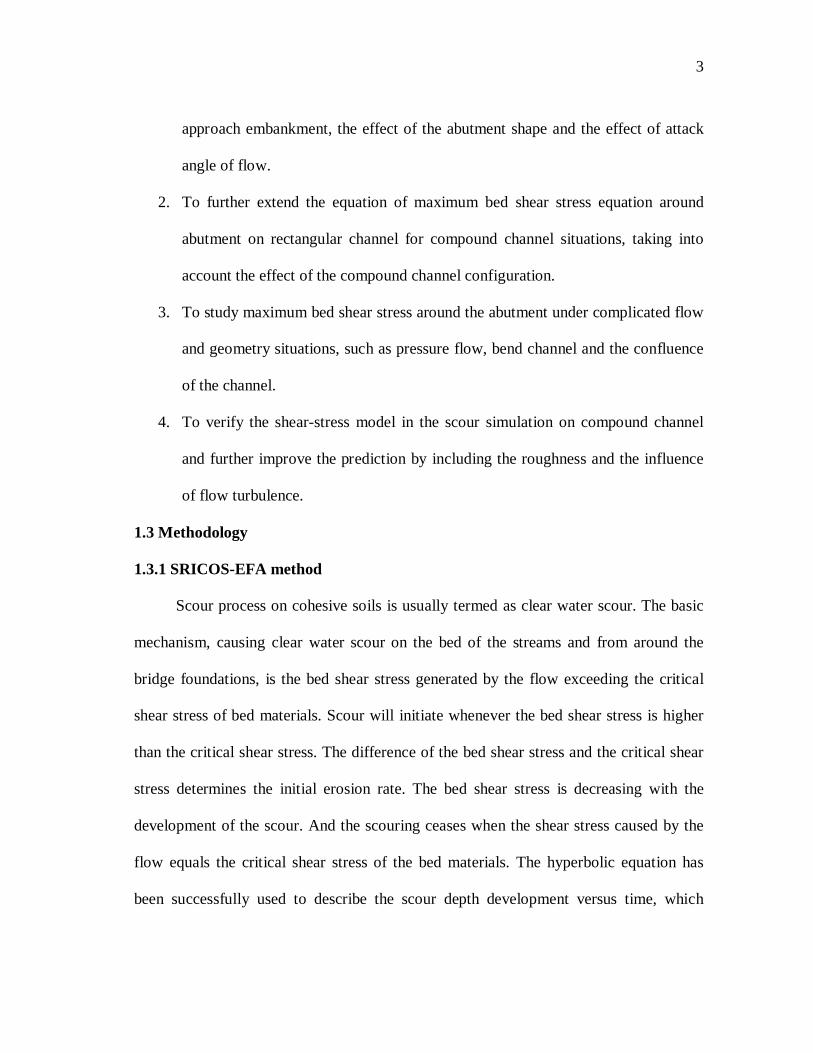
Scour process on cohesive soils is usually termed as clear water scour. The basic
mechanism, causing clear water scour on the bed of the streams and from around the
bridge foundations, is the bed shear stress generated by the flow exceeding the critical
shear stress of bed materials. Scour will initiate whenever the bed shear stress is higher
than the critical shear stress. The difference of the bed shear stress and the critical shear
stress determines the initial erosion rate. The bed shear stress is decreasing with the
development of the scour. And the scouring ceases when the shear stress caused by the
flow equals the critical shear stress of the bed materials. The hyperbolic equation has
been successfully used to describe the scour depth development versus time, which
4
implies that the scour process depends on the initial scour rate and the ultimate scour
depth (Briaud et al. 1999, 2001).
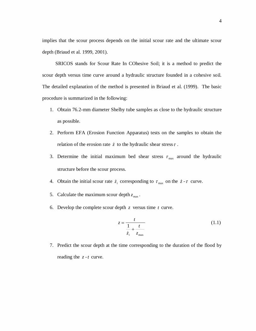
SRICOS stands for Scour Rate In COhesive Soil; it is a method to predict the
scour depth versus time curve around a hydraulic structure founded in a cohesive soil.
The detailed explanation of the method is presented in Briaud et al. (1999). The basic
procedure is summarized in the following:
1. Obtain 76.2-mm diameter Shelby tube samples as close to the hydraulic structure
as possible.
2. Perform EFA (Erosion Function Apparatus) tests on the samples to obtain the
relation of the erosion rate z to the hydraulic shear stressτ .
3. Determine the initial maximum bed shear stress maxτ around the hydraulic
structure before the scour process.
4. Obtain the initial scour rate iz corresponding to maxτ on the z -τ curve.
5. Calculate the maximum scour depth maxz .
6. Develop the complete scour depth z versus time t curve.
max
1z
tz
tz
i
+=
(1.1)
7. Predict the scour depth at the time corresponding to the duration of the flood by
reading the z - t curve.

5
This method has the advantages of being simple, site specific and suitable for
complicated conditions of multi-floods, multilayer soils and has been well verified in the
completed NCHRP 24-15 (Briaud et al., 2003).
1.3.2 CHEN3D program
The CHEN3D (Computerized Hydraulic ENgineering program for 3D flow)
computer program (Chen & Patel 1988, Chen et al. 1990, Chen 2002) is utilized in
current research to perform the numerical simulations. Chimera domain decomposition
approach has been incorporated into CHEN3D for time-domain simulation of the flow
around complex hydraulic configurations. The turbulent flow is performed using the
Reynolds-Averaged form of the Navier-Stokes equations. The entire computational
domain can be divided into two regions in order to facilitate the implementation of two-
layer turbulent model approach. One is the thin layer region around the solid boundary,
applying one-equation turbulence model to account for the wall-damping effects. And
the other one is the fully turbulent region away from the wall, employing the standard
ε−k two equation model to resolve the fully turbulent flow.
1.3.3 Maximum bed shear stress
The primary objective of this research is to determine the maximum bed shear
stress around the abutment in river channel. It is very difficult to measure the bed shear
stress accurately in the flume test. Hence, numerical simulation is utilized to provide τmax
in SRICOS-EFA method. The approach of reference case and correction factors in HEC-
18 is adopted to establish the equation of maximum bed shear stress around abutment.
Dimensional analysis is performed to determine the important parameters to be studied.

6
Flume tests can provide the velocity measurements and the initial erosion rate of the
river bed, which can be used to verify the numerical simulation indirectly.
1.3.4 Scour model
In the present scour prediction method, the scour rate equation is experimentally
obtained from EFA tests. In the numerical simulations, the incremental scour depth is
computed according to the local bed shear stress and the scour rate equation. After the
new scour depth distribution is obtained, the boundary fitted grid is updated
automatically for the next time flow field and bed shear stress calculation. Stream bed
roughness and turbulence properties have also been incorporated into the scour model to
improve the scour development prediction.
1.4 Dissertation Outline
This dissertation consists of a number of numerical studies of the abutment scour
in cohesive soils. The work is divided into three major parts: maximum bed shear stress
around abutment in open channel flow, bed shear stress distribution in complex channel
and pressure flow, and prediction of clear water scour.
An overview of existing knowledge is given in Chapter II. This chapter presents
the literature review of current knowledge in mechanism of scour, bed shear stress study
of pier scour, contraction scour and abutment scour and the advance of the numerical
simulation on clear water scour prediction.
Mathematical formulation is presented in Chapter III. The CHEN3D program
with its boundary conditions is mathematically explained. To close the equation, this
chapter also covers two-layer turbulence model employed in the code. Also, this chapter
7
shows the numerical method, which consists of transformed plane, finite analytic
method, and velocity/pressure coupling. An overall procedure is provided to describe the
algorithm of a computational technique.
Chapter IV presents the numerical studies of maximum bed shear stress around
abutment in open channel flow. The systematic numerical matrix is designed and
conducted. An equation for maximum bed shear stress around a bridge abutment is
proposed, taking into account the effect of water depth, the effect of channel contraction
ratio, the effect of abutment aspect ratio, the effect of abutment shape, the effect of
attack angle and the effect of the compound channel configuration. The proposed
equation of maximum bed shear stress around abutment is verified indirectly according
to the initial erosion rates from the flume tests.
Chapter V presents the numerical studies of bed shear stress distribution on
complex channel geometries and under pressure flow conditions. The studies of the
complex channels include the flow in straight compound channel with different flood
plain elevations on both sides, channel bends of different R/W and abutment location,
and the confluence of upstream channel. The studies of overtopping flow include the
overtopping flow in straight symmetric channel, straight asymmetric channel, and in
channel bends. The influence of the bridge deck and the channel geometry has been
discussed according to the simulation results.
Chapter VI presents the numerical studies on clear water scour prediction. Shear
stress model has been applied in the simulation of flume test cases and modified to
include the influence of roughness and the turbulence effect. The scour development
8
under overtopping conditions is also conducted with the variation of water depth and the
recommendation is proposed.
Chapter VII addresses the conclusions of the dissertation and recommendations
for future research.

9
CHAPTER II
LITERATURE REVIEW OF BRIDGE SCOUR
2.1 Fundamentals of Bridge Scour
Bridge scour is the erosive action of flowing water, excavating and carrying away
material from the bridge contracted streambeds and from around the bridge foundations.
Scour at the bridge contracted zone is one type of contraction scour, which belongs to
general scour; while scour around the bridge foundations is termed as local scour,
including pier scour and abutment scour.
Contraction scour at bridge crossing is due to the reduction of flow area by the
existence of the bridge foundation on river channel. From the continuity law, a decrease
in flow area results in an increase in average velocity and bed shear stress across the
entire contracted channel. Contraction scour initiates when the bed shear stress exceeds
the critical bed shear stress of the bed material. As the bed elevation is lowered, the flow
area increases and the velocity and bed shear stress decrease until the relative
equilibrium is reached again. Contraction scour usually involves removal of material
from the bed across all or most of the channel width.
Local scour at pier or abutment results from the formation of vortices at their
base, which are usually called horseshoe vortex. Water can only pile up to increase
pressure or go down to dig the riverbed when hitting the obstruction like pier or
abutment. Downflow forms the horse shoe vortex, which is the major reason for the
local scour. Increasing of the pressure will accelerate the flow around the bridge

10
foundation and take away the eroded material. In addition to the horseshoe vortex
around bridge foundation, there are vertical vortices at downstream called the wake
vortex. Wake vortices also contribute to the removal of bed material around bridge
foundation. However, the wake vortices behind the bridge foundation will diminish
rapidly as the downstream distance increases.
Factors affecting local scour at bridge foundation include the approaching flow,
the bridge foundation configuration and channel geometry. Extensive researches have
been done to study these influence. The observations are summarized as follows.
The influence of approaching flow comes from approaching velocity and
approaching water depth. The higher the velocity, the deeper the local scour. However,
the scour depth will increase with the water depth only when the water depth is relatively
shallower than the size of the bridge foundation. For bridge pier, the water depth will
have no influence when the water depth is larger than two times of the bridge diameter.
For abutment, the influence will also depend on the size of the abutment.
The influence of bridge foundation configuration usually includes the projected
foundation length normal to the flow, the shape of the nose of a pier or abutment, the
attack angle of flow to the pier or abutment. For pier, the scour depth will increase with
the increase of the projected length. But, the increment is smaller and smaller when the
project length is larger and larger. The projected length of the abutment is not always a
good measure for the local scour depth around abutment, especially when the abutment
is very long and setting on the floodplain. The shape of the bridge foundation can have
up to a 20 percent influence on the scour depth. And the attacking angle of the flow to

11
the bridge foundation also has a significant effect on the scour depth, which can be up to
20 percent.
Channel geometry here is classified as rectangular channel or compound channel
and straight channel or bend channel. The study of channel geometry on the local scour
is not as extensive as the flow condition and the bridge foundation configuration. Most
of the testing is conducted on straight rectangular channel. The flow field in the straight
rectangular channel is usually very uniform; while the bend channel and the compound
channel can redistribute the flow and further change the channel conveyance capacity at
the different section of the channel.
Scour can be identified as live-bed scour and clear-water scour according to the
sediment transport characteristics. Live bed scour occurs when there is import of the bed
material from upstream reach into the crossing. Live scour is cyclic in nature; the scour
hole that develops during the rising stage of a flood refills during the falling stage. Clear-
water scour occurs when there is no refill or deposition at the crossing. In such a case,
the scour hole will not be refilled once the materials removed. This dissertation is the
study of abutment scour on cohesive soils. So, all the contents about scour simulation
will focus on clear water scour.
The scour problem has been systematically documented in HEC-18 (Richardson
& Davis, 2001). Only the fundamental of bridge scour is summarized here.
2.2 Bed Shear Stress at the Bridge Crossing
Open channel flow may be laminar, transitional or turbulent. What type of flow
occurs depends on the Reynolds number, ν/Re hVR= , where V is the average velocity
12
, hR is the hydraulic radius of the channel and ν is the kinematic viscosity of water. The
general rule is that open channel flow is laminar if 500Re< , turbulent if 500,12Re > ,
and transitional otherwise. In fact, typical Reynolds numbers are quite large, well above
the transitional value and into the wholly turbulent regime. The channel resistant force is
independent of Reynolds number, dependent only on the relative roughness.
The resistant force in the constant depth channel flow has been studied many
years ago. Under the assumption of steady uniform flow, the bed shear stress can be
determined by the unit weight of waterγ , hydraulic radius hR and the energy slope S as
following (Munson et al., 1998)
SRhγτ = (2.1)
Manning’s equation (in SI unit) provides the dependence of average channel
velocity V on the hydraulic radius hR and the energy slope S ,
nSR
V h2/13/2
= (2.2)
The parameter n is the Manning’s resistance coefficient. Its value is dependent on
the surface material of the channels’ wetted perimeter and is obtained from experiments,
having the unit of 3/1/ms .
Hence, the popular used bed shear stress equation in open channel flow can be
derived by substituting equation (2.2) into equation (2.1),
3/122 −= hRVnγτ (2.3)

13
Contraction scour means the uniform bed elevation change across the entire
contracted channel. The scour depth at the center of the channel is usually chosen to be
the representative value. The bed shear stress at the constricted channel center will still
follow the same rule of the open channel flow and the influence of viscous force can be
ignored. All the influence of the bridge foundation can be involved by the correction of
the average velocity in equation (2.3).
Nurtjahyo (2003) numerically studied the maximum bed shear stress at the center
of the channel under long contraction. The equation is generated by correcting the open
channel flow equation (2.3), including the effect of the contraction ratio Rck − , the effect
of contraction transition angle θ−ck , the effect of the contraction length Lck − .
31
22max_
−
−−−= hLccRccontr RVnkkk γτ θ (2.4)
75.1
2
138.062.0
+=− B
Bk Rc
5.1
909.01
+=−θ
θck
<
−
−
−
+
≥
=−
−
− 35.0,98.136.177.0
35.0,12
2121Lc
Lc
Lc kforBB
LBB
L
kfor
k
where, γ is the unit weight of water, n is the Manning’s coefficient, hR is hydraulic
radius, V is the upstream averaged velocity, 1B is the upstream channel width, 2B is the

14
channel width at the contracted zone, L is the length of the contracted zone, θ is the
contraction transition angle.
For local bridge scour, like pier scour and abutment scour, the location of scour
hole is right around the hydraulic structures. The bed shear stress features will be quite
different from the preceding open channel bed shear stress. Bridge foundation will come
in and affect the magnitude and the distribution of the bed shear stress. Besides those
affecting factors in the open channel flow, the geometry and the setting of the bridge
foundations will also strongly affect the local bed shear stress. In the analysis of the open
channel flow, the viscous force (represented by Reynolds number) is ignored. Here, on
local scour analysis, it is going to be the dominant factor.
Many researchers have studied the flow structure at bridge foundations and found
out the similarity of the flow in and around the scour hole at pier and abutment,
especially when the abutment is relatively short compared with the water depth
(Melville, 1997). This implies that the bed shear stress should also have the similar trend
around bridge pier and abutment.
Hjorth (1975) investigated the bed shear stress around circular pier. Two circular
piers of 0.05m and 0.075m diameter were used in the flume test, combined with two
different velocities of 0.15m/s and 0.30m/s and two different approach depths of 0.1m
and 0.2 m. A hot-film probe was used to measure bed shear stress on the rigid flume bed.
Hjorth tried to correlate the local maximum bed shear stress around pier with the
approach bed shear stress and found the amplification factor of approachττ /max ranging
from 5 to 11 for a circular pier.
15
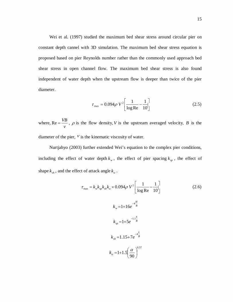
Wei et al. (1997) studied the maximum bed shear stress around circular pier on
constant depth cannel with 3D simulation. The maximum bed shear stress equation is
proposed based on pier Reynolds number rather than the commonly used approach bed
shear stress in open channel flow. The maximum bed shear stress is also found
independent of water depth when the upstream flow is deeper than twice of the pier
diameter.
−=
101
Relog1094.0 2
max Vρτ (2.5)
where,v
VB=Re , ρ is the flow density, V is the upstream averaged velocity, B is the
diameter of the pier, ν is the kinematic viscosity of water.
Nurtjahyo (2003) further extended Wei’s equation to the complex pier conditions,
including the effect of water depth wk , the effect of pier spacing spk , the effect of
shape shk , and the effect of attack angle αk .
2max
1 10.094log Re 10w sp shk k k k Vατ ρ
= × −
(2.6)
BH
w ek4
161−
+=
BS
sp ek1.1
51−
+=
BL
sh ek4
715.1−
+=
57.0
905.11
+=α
αk

16
where, v
VB=Re , ρ is the flow density, V is the upstream averaged velocity, H is
upstream water depth, B is the pier diameter, S is the pier spacing, L is the length of
the pier in the flow direction, α is the flow attach angle.
Awazu (1967) proposed an equation for estimating maximum bed shear stress
around a thin rectangular plate from 12 flume tests. Froude number was varied from
0.488, 0.508 to 0.526 and the opening ratio of channel was changed between 0.1 and 0.4.
Awazu found that the blockage ratio affects the bed shear stress around spur dikes
significantly, while the effect of the Froude number is negligible. The maximum
amplification of approachττ max is about 3.8 in his experiments. The maximum bed shear
stress amplification around spur dikes is,
021.014.1log max10 −
−=
Bb
approachττ (2.7)
where maxτ is maximum bed shear stress around spur dike, appraochτ is approach bed
shear stress, b is spur dike protrusion length, B is the channel width.
Zaghloul (1974) related bed shear stress around spur dike to the average velocity,
and local vorticity. He proposed an empirical equation as
++= 212 1 KKV
C noseωωγτ (2.8)
where τ is bed shear stress, γ is the unit weight of water, V is the average velocity, ω
is the vorticity at the point, noseω is the vorticity at the spur dike nose, C is the Chezy’s
17
coefficient, 1K and 2K are the empirical constants. 1K = 0.5 and 2K is from 0 to 0.2
depending on the distance from the dike.
Rajaratman & Nwachuku (1983) reported 13 measurements of bed shear stress
around groin-like structures. The amplification factor approachττ /max increases
significantly from 3.0 to 4.5 when the blockage ratio varies from 0.08 to 0.16, whereas
the influence of Froude number is negligible. The cylindrical pier was found to have
slightly smaller amplification factor than that of the thin plate. However, the disturbed
area is much smaller from cylindrical pier than from thin plate.
Tingsanchali & Maheswaran (1990) proposed an equation to calculate the bed
shear stress around the groin according to the depth averaged velocity. A 2-D numerical
simulation of depth-averaged ε−k turbulence model was used to study the effect of
streamline curvature and establish the correction factor near the groin.
( )[ ] 5.00
23/122 2tan1 αγτ += −yVn (2.9)
where τ is the bed shear stress, γ is the unit weight of water, n is Manning’s
coefficient V is the depth averaged velocity , y is the flow depth , 0α is the turning
angle between the surface streamline direction and the upstream approaching direction.
Molinas et al. (1998) proposed a maximum bed shear stress equation around
abutment based on 15 experiments with vertical wall abutment on rectangular channel.
The maximum bed shear stress around abutment maxτ is taken as the summation of the
shear stress at the contraction zone contτ and the shear stress increment due to abutment
alone *maxτ . From the testing, the contribution from channel contraction is negligible
18
when the length of the abutment is relatively short compared with the channel width.
The equation is given below:
*maxmax τττ += cont (2.10)
+
=
5
432
1 1c
acapp
c
app
cont
yL
FRcRc
ττ
1tan1 220
*max −+= ωατ
τRm
app
=
3
21
mam
app yL
Fmωα
where 1c , 2c , 3c , 4c , 5c , 0m , 1m , 2m , 3m are experimentally determined coefficients,
LLR a−=1 is the opening ratio, aL is the length of the abutment, L is the half width of
the channel, appF is the approached Froude number, y is the upstream water depth.
Nurtjahyo (2003) proposed the equation for the prediction of the maximum bed
shear stress around abutment based on the correction of the open channel flow equation.
The effect of the contraction and the effect of the contraction transaction angle are
considered. He stated that the effect of the water depth has been included in the open
channel flow equation; and the contraction length of the channel has little influence on
the maximum bed shear stress around abutment.
1
2 2 3max_ abut a R a a y a L hk k k k n V Rθτ γ
−
− − − −= (2.11)
5.05.12
1 −=− BBk Ra
19
2
90909.11
−
+=−
θθθak
1≈−Lak
1≈−Hck
where, γ is the unit weight of the flow, V is the upstream averaged velocity, n is
Manning’s coefficient, hR is hydraulic radius, 1B is the upstream channel width, 2B is the
channel width at the contracted zone, L is the length of the contracted zone, θ is the
contraction transition angle.
When flooding, the bridge deck may become partially or entirely submerged.
Pressure flow occurs when the water surface exceeds the low chord of the bridge deck.
And the floodwater is forced through under the bridge deck. Blockage ratio of the
channel keeps increasing until the water surface begins to overtop the bridge deck. When
the bridge deck totally submerged, the deck behaves like a broad crested weir. The flow
changes from exclusively pressure flow to a combined weir and pressure flow. Pressure
flow causes the increase of velocity under the bridge deck and further increase the bed
shear stress and bridge scour. Studies of scour in pressure flow are still in the early stage.
Abed (1991) first studied the clear water pier scour in pressure flow and found the scour
depth 2.3-10 times greater than free surface pier scour; Jones et al (1993) extended
Abed’s study to isolate the deck scour from pier scour. One important finding is the
magnitude of pier scour component under pressure flow as same as under free surface
flow conditions. Jones suggested the components of pressure flow vertical deck
contraction scour and the pressure flow pier scour be additive. Umbrell et al (1998)
20
analyzed the data in Jones’ study and further improved the vertical deck contraction
equation in pressure flow. Arneson (1997) proposed an equation for vertical deck
contraction scour based on the similar flume tests study to Jones. ABSCOUR USERS
MANUAL (2007) suggests 10% increase of the abutment scour depth when the
approach water depth is equal to or greater than 1.2 of the distance of the height of the
low chord above the riverbed. The limited literatures are all about the scour depth
studies. As for the variation of the bed shear stress around bridge foundation under
pressure flow is still unknown.
Laboratory studies of bridge scour have been extensively conducted on constant
depth channel for simplicity while this is rare in the real world. Typical cross sections in
rivers consist of a deep main channel and one or both sides of relatively shallow
floodplain. Flood plain is often rougher than main channel. Consequently, velocities tend
to be significantly greater in main channel than on floodplain. The velocity discrepancy
between the main channel and flood plain causes the lateral momentum transfer and
secondary circulation. The flood plain and main channel flow interaction have been
studies by lots of researchers, Rajaratnam & Ahmadi (1979), Knight & Demetriou
(1983), Myers & Brennan (1990), Wormleaton & Merrett (1990) and Naot et al. (1993).
However, the velocity in flume test is generally uniformly distributed even for
compound channel configuration. Hence, the geometric blockage of the abutment in the
flume test will be very close to the discharge blockage; while in real rivers the geometric
blockage is significantly different from the actual discharge blockage caused by the
21
abutment. The equations proposed based on the geometric blockage in the flume tests
tend to overestimate the scour depth if the geometric blockage is used in the real cases.
2.3 Issues in the Numerical Simulation of Bridge Scour on Cohesive Soils
3D numerical simulation of bridge scour is a very young topic in the history of
bridge scour study. It is a promising tool for the study of the interaction between flow
field and soil erosion process. Its development depends on both the computational fluid
dynamics and the soil erosion model. When talking about bridge scour on cohesive soils,
it usually means clear water scour. The sediment transport equation will not be solved
together with the fluid calculation. As for the erosion rate function of the cohesive soils,
the current model is only limited to the simple shear stress model. The parameters appear
in the model are the bed shear stress and the critical shear stress of the soils. Both of the
CFD technique and the soil erosion model are under quick development now.
Wei et al. (1997) numerically studied pier scour process in cohesive soils. The
scour rate was assumed to be a linear function of the streambed shear stress. The
important flow features, such as horseshoe vortex in front of the pier and the wake
vortices behind the pier, were observed in the simulation. Simulations showed the
reasonable prediction of the time history of scour depth with the tuned erosion rate
function.
Chen (2002) conducted the bridge scour simulations for the model scale complex
rectangular pier configuration and the prototype complex circular pier configuration. The
erosion rate is assumed linear with bed shear stress. Both of the global and local pier

22
scour have been observed in the simulations. This shows the applicability of the
tridimensional numerical simulation in the real complicated engineering problems.
Jiang et al. (2004) applied the shear stress model in the estimation of contraction
scour of firm clay riverbed. The erosion function of the cohesive soils is determined
through a rotating cylinder device called SERF (Simulator of Erosion Rate Function).
The linear shear stress model combined with the 3D shallow water hydrodynamic code
was applied for the 5km river channel and yielded good agreement of scour depth
prediction with the measurement.
2.3.1 Critical shear stress of the cohesive soils
Critical shear stress for cohesionless soils has been studies extensively by
researchers and many equations have been proposed and applied in practice. It depends
mainly on the size of the soil particles. While the critical shear stress for cohesive soils
relates more to the cohesive force existing between the fine particles. The initiation of
cohesive soils is more complex than cohesionless soils. Research indicates that the
critical shear stress is influenced by the following parameters: Cation Exchange Capacity
(CEC), Salinity, Sodium Adsorption Ratio (SAR), PH-level of pore water, temperature,
w%, r, PI, Su, e, swell, D50, %200, clay mineral, dispersion ratio, turbulence, water
chemical component, etc. (Winterwerp 1989, Cao 2001,).
Mirtskhoulava (1988) stated the two steps of the erosion of clay: (1) Initially,
loosened particles and aggregates with weakened bonds to the other parts are removed in
a short period. This process is very similar to the erosion of cohesionless soils and leads
to a rougher surface. (2) The bonds between aggregates are destroyed gradually by the

23
pulsating drag and lift forces caused by the turbulent flow. And the aggregate will be
carried away simultaneously when the holding cohesion force disappears.
Dunn (1959) studied the correlation of critical shear stress of soils to the vane
shear strength experimentally. He concluded that the critical shear stress increases with
the increase of the clay content and proposed the critical shear stress equation as
following,
θθ
τ tan18.01000
tan02.0 ++= v
cS (2.12)
where vS is the vane shear strength, and θ is the slope of the linear relation between
critical shear stress and vane shear strength.
Smerdon and Beasley (1959) investigated the influence of plasticity index,
dispersion ratio, and mean particle size of clay on the critical shear stress by conducting
flume tests. The relation between the critical shear stress, cτ , and the plasticity index,
PI , and Middleton’s dispersion ratio, rD , were given by
( ) 84.00034.0 PIc =τ (2.13)
( ) 63.0213.0 −= rc Dτ (2.14)
Ivarson (1998) proposed the relation between critical shear stress cτ , unconfined
compressive strength of clay soils uS , and mean average velocityV , based on the stream
stability criteria for cohesive soils by Flaxman as:
12.11log 28.67uc
SV
τ −= (2.15)
where, all terms are in English units;
24
Briaud et al (1999) argued the critical shear stress does not theoretically exist.
However, he believed that the concept of critical shear stress is practically useful and
future suggested that cτ should be defined in the way based on a standardized small
scour rate. This threshold scour rate is proposed as 1 mm/hr in the application of EFA
(erosion function apparatus). The research also showed that large variance in the
predicted cτ among different researchers, from 0.02 to 100 Pa. Hence, they
recommended to measure cτ directly from EFA test.
2.3.2 Erosion rate of soils
The scour around bridge foundation can reach the equilibrium scour depth in
cohesionless soils for just one flood since gravity is the mainly dominant factor. While it
may take several floods to reach the final scour depth in cohesive soils and last about
tens or hundreds of years. All those factors mentioned above affecting the critical shear
stress in cohesive soils will continue to control the erosion rate of the cohesive soils.
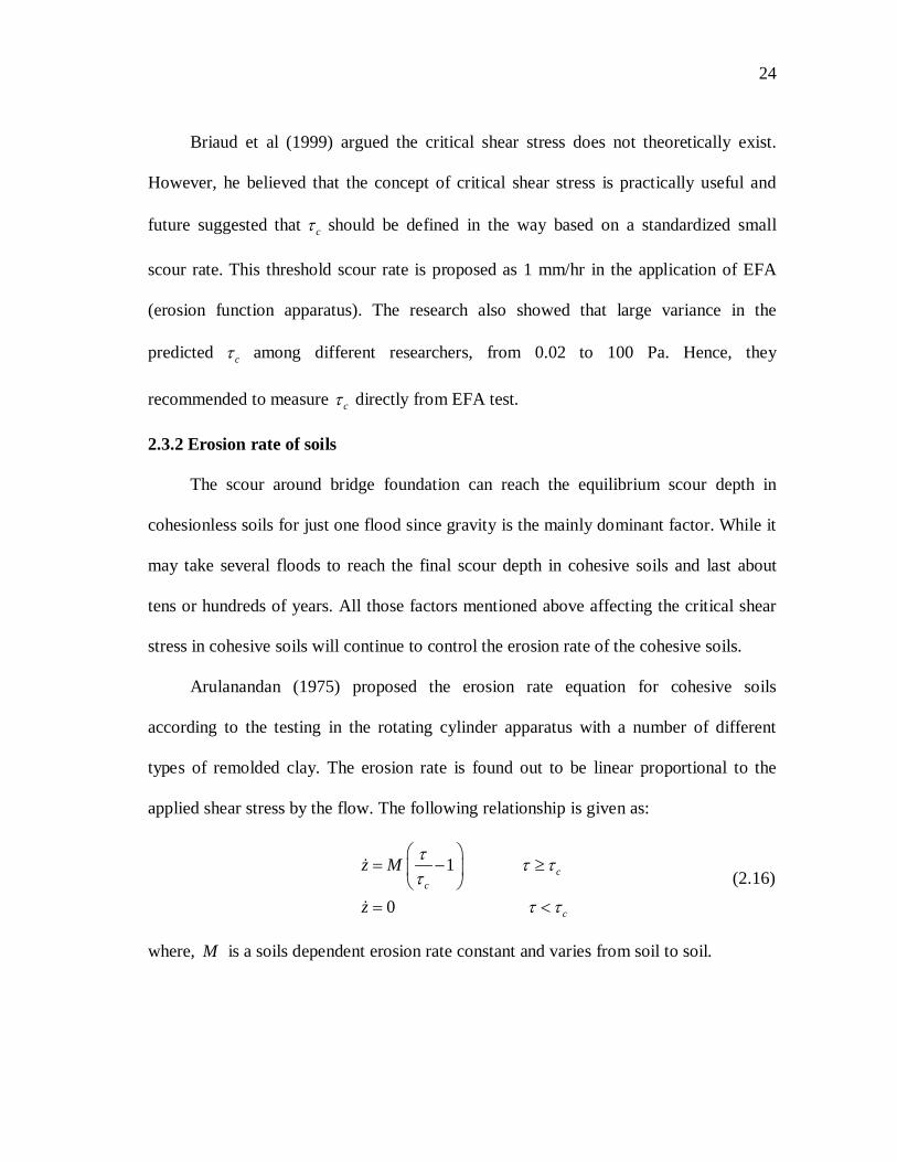
Arulanandan (1975) proposed the erosion rate equation for cohesive soils
according to the testing in the rotating cylinder apparatus with a number of different
types of remolded clay. The erosion rate is found out to be linear proportional to the
applied shear stress by the flow. The following relationship is given as:
1
0
= − ≥
= <
cc
c
z M
z
τ τ ττ
τ τ
(2.16)
where, M is a soils dependent erosion rate constant and varies from soil to soil.
25
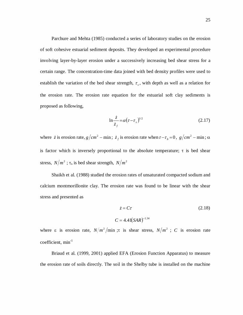
Parchure and Mehta (1985) conducted a series of laboratory studies on the erosion
of soft cohesive estuarial sediment deposits. They developed an experimental procedure
involving layer-by-layer erosion under a successively increasing bed shear stress for a
certain range. The concentration-time data joined with bed density profiles were used to
establish the variation of the bed shear strength, sτ , with depth as well as a relation for
the erosion rate. The erosion rate equation for the estuarial soft clay sediments is
proposed as following,
( ) 2/1ln sfz
z ττα −=
(2.17)
where z is erosion rate, min2 −cmg ; fz is erosion rate when 0=− bττ , min2 −cmg ; α
is factor which is inversely proportional to the absolute temperature; τ is bed shear
stress, 2mN ; τs is bed shear strength, 2mN
Shaikh et al. (1988) studied the erosion rates of unsaturated compacted sodium and
calcium montmorillonite clay. The erosion rate was found to be linear with the shear
stress and presented as
z Cτ= (2.18)
( ) 34.141.4 −= SARC
where ε is erosion rate, min2mN ;τ is shear stress, 2mN ; C is erosion rate
coefficient, min-1
Briaud et al. (1999, 2001) applied EFA (Erosion Function Apparatus) to measure
the erosion rate of soils directly. The soil in the Shelby tube is installed on the machine

26
and pushed out 1mm into the conduit by the piston as fast as it takes to erode the soil by
water flowing over it. Erosion rate is recorded through the vertical shortness of the soil
column per unit time with the corresponding flow velocity. And the shear stress could be
evaluated from Moody Chart.
2.3.3 Effect of roughness
The influence of river bed roughness on the flow field can be separated into (1)
particle resistance accounting for the interaction between the flow and the individual
particles and (2) form resistance due to bedform configurations. The study of the particle
roughness has been studies decades ago. And the most well known result was done by
Nikuradse (1933) (see, Cebeci and Bradshaw, 1977) in pipe flows with sand-roughened
surface. The principal result from the data of Nikuradse is the velocity distribution near a
rough wall has the same slope (giving the same Karman constant,κ ) as on smooth wall,
but different intercepts, B∆ :
BByu ∆−+= ++ ln1κ
(2.19)
where τuUu =+ , ντ yuy =+ , y is the distance from the wall, κ =0.418, B is the
additive constant (for pipe, 45.5=B and for open channel, 2.5=B ), B∆ is a function of
( )ντukk ss =+ , sk is the surface roughness.
Ioselevich and Pilipenko (1974) (see, Cebeci and Bradshaw, 1977) gave the
analytic fit to the data of Nikuradse:
27
( )[ ]
>+−
<≤−
+−
<
=∆
++
+++
+
90,ln15.8
9025.2,811.0ln4258.0sinln15.8
25.2,0
ss
sss
s
kkB
kkkB
k
B
κ
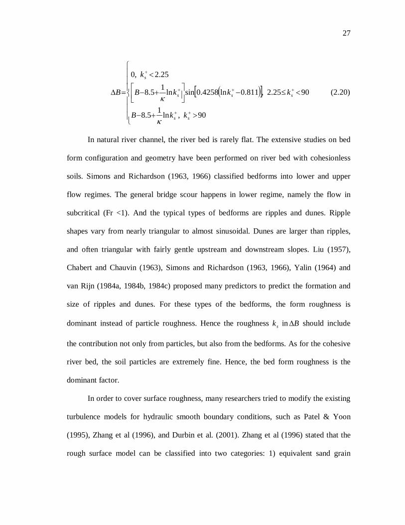
κ (2.20)
In natural river channel, the river bed is rarely flat. The extensive studies on bed
form configuration and geometry have been performed on river bed with cohesionless
soils. Simons and Richardson (1963, 1966) classified bedforms into lower and upper
flow regimes. The general bridge scour happens in lower regime, namely the flow in
subcritical (Fr <1). And the typical types of bedforms are ripples and dunes. Ripple
shapes vary from nearly triangular to almost sinusoidal. Dunes are larger than ripples,
and often triangular with fairly gentle upstream and downstream slopes. Liu (1957),
Chabert and Chauvin (1963), Simons and Richardson (1963, 1966), Yalin (1964) and
van Rijn (1984a, 1984b, 1984c) proposed many predictors to predict the formation and
size of ripples and dunes. For these types of the bedforms, the form roughness is
dominant instead of particle roughness. Hence the roughness sk in B∆ should include
the contribution not only from particles, but also from the bedforms. As for the cohesive
river bed, the soil particles are extremely fine. Hence, the bed form roughness is the
dominant factor.
In order to cover surface roughness, many researchers tried to modify the existing
turbulence models for hydraulic smooth boundary conditions, such as Patel & Yoon
(1995), Zhang et al (1996), and Durbin et al. (2001). Zhang et al (1996) stated that the
rough surface model can be classified into two categories: 1) equivalent sand grain
28
roughness models;2) topographic form-drag models. Patel (1998) pointed out that the
turbulence model for roughness surface should consider two factors: (a) the model has
the capability to classify three roughness regions, i.e. hydraulic smooth, transitional, and
fully-rough surfaces, and (b) the model has the capability to describe separated flow.
Patel & Yoon (1995) proposed the roughness turbulence model based on the
modifying of mixing length in two layer ε−k model. The roughness effect could be
included easily by changing the boundary conditions in ω−k model. By comparing these
two models, they concluded that the ω−k model of Wilcox is better than the modified
ε−k model. And the modified ε−k model needed further tune of the constants and
dumping functions in the length-scale equations.
Zhang et al. (1996) built a new-low-Reynolds-number ε−k model to simulate
turbulence flow over smooth and rough surfaces. He continued to adopt the equivalent
sand grain roughness concept and modified reduction factors in the low Reynolds
number models. They showed the model is capable of predicting the log-law velocity
profile, friction factors, turbulent kinetic energy and dissipation rate by comparing it
with experiments.
Durbin et al. (2001) presented a modified two-layer ε−k model. The new model
modified the mixing length formula by adding a hydrodynamic roughness length into the
wall distance and also modified the boundary condition for turbulence kinetic energy.
2.3.4 Effect of turbulence intensity
Nurtjahyo (2003) stated that the bridge scour simulation with shear stress model
could not predict the scour pattern correctly, even if the scour depth was reasonable

29
compared with the flume tests. Li (2002) observed the deep scour at lee side of the
circular pier. The bed shear stress at downstream of pier is pretty small; while the
turbulent intensity is significant. This implies that the flow turbulence can contribute to
the increase of the erosion ratio as well as bed shear stress. Nurtjahyo (2003) added the
turbulence kinetic energy term into the erosion rate equation and improved the scour
pattern prediction in the clear water pier scour simulations.
Dufresne et al (2007) investigated the influence of both the bed shear stress (BSS)
and bed turbulent kinetic energy (BTKE) on the sedimentation and mass separation in
storm-water tank pilot. The authors found out that BSS can only be used for no overflow
cases; while BTKE should be chosen for overflow cases. Neither of them can predict the
measurement well for both conditions.
The study of the effect of turbulence on the scour is still in the early stage. Only
few literatures can be found very recently. It is believed that the turbulence affects the
whole scour process and contributes to both the final scour depth and scour pattern.
30
CHAPTER III
GOVERNING EQUATIONS FOR CHEN3D PROGRAM
CHEN3D (Computerized Hydraulic ENgineering program for 3D flow) has been
employed in conjunction with chimera domain decomposition approach for time-domain
simulation of flow around complex hydraulic configurations. The turbulent flow is
performed using the Reynolds-Averaged form of the Navier-Stokes equations. The entire
computational domain can be divided into two regions in order to facilitate the
implementation of two-layer turbulent model approach. One is the thin layer region
around the solid boundary, applying one-equation turbulence model to account for the
wall-damping effects. And the other one is the fully turbulent region away from the wall,
employing the standard ε−k two equation model to resolve the fully turbulent flow. The
formulation has been described in detail in Chen and Patel (1988) and Chen and Korpus
(1993). The CHEN3D program has been further developed to include the roughness and
scour model in current research to simulate the clear water scour. The approach by Patel
and Yoon (1995) is used to capture the effect of roughness. And the method proposed by
Nurtjahyo (2003) is implemented to perform the scour development. A summary of the
approach is given below.
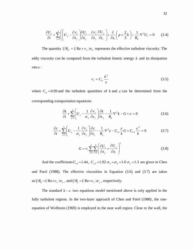
3.1 Governing Equations for Hydrodynamics
The non-dimensional Reynolds-Averaged Navier-Stokes equations for
incompressible, viscous flow in Cartesian coordinates ( )tzyxtxi ,,,),( = are as follows:
31
03
1=
∂∂∑
=i i
i
xU
(3.1)
0Re1 2
3
1=∇−
∂∂
+
∂
∂+
∂∂
+∂∂ ∑
=i
ij j
ji
j
ij
i Uxp
xuu
xU
Ut
U (3.2)
Equation (3.1) represents the continuity equation and equation (3.2) represents the
momentum equations. ),,( WVUUi = and ),,( wvuui = represent Cartesian components of
the mean and the fluctuating velocities, t is time, p is pressure, ν/Re 0 BU= is the
Reynolds number based on the characteristic length B , the reference velocity 0U , and the
kinematics viscosityν . All quantities in the above equations, and those follows, are
made dimensionless by 0U , B and fluid density ρ . Body force is ignored here. For open
channel flow, the influence of gravity can be considered on the free surface boundary
conditions.
In equation (3.2), the six additional Reynolds stresses terms jiuu− make the
equations unsolvable without additional equations. Based on the assumption of
Boussinesq, the Reynolds stresses can be expressed in terms of an isotropic eddy
viscosity tv and the mean rate of strain, which is analogous to the molecular viscosity.
The Reynolds stresses can then be written as:
kxU
xU
uu ijij
ji
tji δν32
−
∂
∂+
∂∂
=− (3.3)
where ( ) 2/wwvvuuk ++= is the turbulent kinetic energy and ijδ is the Kronecker delta.
Substituting into (3.2) yields:
32
∑=
=∇−
+
∂∂
+
∂
∂
∂∂
−∂∂
∂∂
−+∂∂ 3
1
2 0132
ji
Uii
j
j
t
j
i
j
tj
i UR
kpxx
Uxx
Ux
Ut
U νν (3.4)
The quantity UtUR σν+= Re11 represents the effective turbulent viscosity. The
eddy viscosity can be computed from the turbulent kinetic energy k and its dissipation
rateε :
ε
ν µ
2kCt = (3.5)
where 09.0=µC and the turbulent quantities of k and ε can be determined from the
corresponding transportation equations:
011 23
1=+−∇−
∂∂
∂∂
−+∂∂ ∑
=
εν
σGk
Rxk
xU
tk
kjj j
t
kj (3.6)
011 2
212
3
1=+−∇−
∂∂
∂∂
−+∂∂ ∑
= kCG
kC
RxxU
t jj j
tj
εεεενσ
εεε
εε
(3.7)
∑∑= =
∂
∂+
∂∂
=3
1
3
1
2
j i i
j
j
it x
UxU
G ν (3.8)
And the coefficients 44.11 =εC , 92.12 =εC 0.1== ku σσ 3.1=εσ are given in Chen
and Patel (1988). The effective viscosities in Equation (3.6) and (3.7) are taken
as ktkR σν+= Re11 , and εε σν tR += Re11 , respectively.
The standard ε−k two equations model mentioned above is only applied in the
fully turbulent regions. In the two-layer approach of Chen and Patel (1988), the one-
equation of Wolfstein (1969) is employed in the near wall region. Close to the wall, the
33
dissipation rate is determined from the turbulent production and the dissipation length
scale, rather than being solved from equation (3.7):
ε
εl
k 2/3
= (3.9)
( )[ ]εε ARyCl yl /exp1 −−= ; ykRy Re= (3.10)
The inner layer was specified when the parameter 1000300 −≤=+ ντ yUy ,
where y is the dimensionless normal distance from the wall and ρττ /wU = is the
friction or shear velocity. Using this relationship, the turbulent production can be
determined from equation (3.6). The eddy viscosity is then found from:
µµ lkCvt = (3.11)
( )[ ]µµ ARyCl yl /exp1 −−= (3.12)
The constants 75.0−= µκCCl , 70=µA , lCA 2=ε and 418.0=κ are given in Chen
and Patel (1988) and chosen to yield a smooth transition of eddy viscosity between the
two regions.
The above one equation model for the inner layer is based on the assumption of a
hydrodynamic smooth wall. Patel and Yoon (1995) extended the model to a rough wall
by modifying the two length scales:
( )
∆+−−∆+=
µµ A
RRyyCl yy
l exp1)( (3.13)
( )
∆+−−∆+=
εε A
RRyyCl yy
l exp1)( (3.14)
34
ykRy ∆=∆ Re (3.15)
The y∆ is normalized by shear velocity τU and kinematics viscosity ν to yield
ντ /yUy ∆=∆ + , and +∆y is related to the roughness of the wall and expressed by:
−−=∆
++++
6exp9.0 s
ssk
kky (3.16)
where τUkk ss Re=+ , and sk is the dimensionless height of the sand grain. In case of
non-uniform sand, sk is usually taken as the median diameter 50D .
To facilitate the coding of the program, the transportation equations for iU , k and
ε are rewritten in the general form:
φφ
φφφν
σφ s
txxUR
jj
tj +
∂∂
+∂∂
∂∂
−=∇12 (3.17)
where φ represents any of the transport quantities iU k and ε . The source functions φs
are:
∂
∂
∂∂
−
+
∂∂
= ∑=
3
132
j i
j
j
t
iUU x
Ux
kpx
Rsi
ν (3.18)
( )ε−−= GRs kk (3.19)
( )εεεεε 21 CGC
kRs e −−= (3.20)
To accurately solve the flow around the boundary of complex geometries, the
boundary fitted coordinate system is used in CHEN3D. Hence, the Cartesian coordinate
( )tzyxtxi ,,,),( = employed in the physical space, has to be transformed to a general

35
curvilinear coordinate system ( ) ( )τζηξτξξξ ,,,,,, 321 = . The vector operations in the
transformed coordinates are:
∑= ∂
∂=
∂∂
=∇3
1
1)(j
jj
ii
i bJx ξ
φφφ (3.21)
∑∑ ∑∑∑ ∑= = == = = ∂
∂+
∂∂
=∂∂
Γ+∂∂
=∇3
1
3
1
3
1
23
1
3
1
3
1
22 )(
i j jj
jji
ij
i j ll
lijji
ij fggξφ
ξξφ
ξφ
ξξφφ (3.22)
∑∑= = ∂
∂∂∂
−∂∂
=∂∂ 3
1
3
1
1i j
jij
ix
bJt ξ
φττ
φφ (3.23)
∂
∂
∂∂
−∂∂
∂
∂=
∂∂
= nj
mk
nk
mj
i
lli
xxxxx
Jbξξξξ
ξ (3.24)
( )∑=
−==3
12
1p
njmknkmjip
lp
li ggggJ
bbg (3.25)
( )∑∑∑== = ∂
∂=Γ−=∇=
3
1
3
1
3
1
2 1j
ijj
m n
imn
mnii JgJ
gfξ
ξ (3.26)
∑= ∂
∂∂∂
=3
1mj
mi
mij
xxg
ξξ (3.27)
21233
21322
22311231312332211
2 )()()(2)det( gggggggggggggJ ij −−−+== (3.28)
where lib , lig , and if are the geometric coefficients. Using these relationships, equations
(3.1) and (3.17) are transformed into:
∑∑∑ ∑∑= == = =
=∂∂
=∂∂
∂∂
=∂∂ 3
1
3
1
3
1
3
1
3
10)(1
i ji
jij
i i jji
i
j
i
i UbJ
Uxx
Uξξ
ξ (3.29)
∑=
+∂∂
=
∂∂
−∂∂
∂3
1j
2
2j
jj
jjj SRag φφφ τ
φξφ
ξξφ
(3.30)
where
36
∑ ∑= =
−
∂∂
−∂∂
−=3
1
3
1
12n
j
m m
tmj
nn
jn
j fbJ
xUb
JR
aξν
στ φ
φφ (3.31)
∂∂
∂+
∂∂∂
+∂∂
∂−= 32
223
31
213
21
2122
ξξφ
ξξφ
ξξφ
φφ gggsS (3.32)
∑∑ ∑= = =
∂
∂+
∂∂
=3
1
3
1
23
1
121
j i lljl
ilil
jt
Ub
Ub
JG
ξξν (3.33)
∑ ∑ ∑∑= = ==
∂
∂
∂∂
−
+
∂∂
=3
1
3
1
3
1
3
1
1132
l j lljl
il
ltl
jUlli
UU
Ub
Jb
JRkpb
JR
si ξξ
νξ
(3.34)
( )ε−−= GRs kk (3.35)
( )εεεεε 21 CGC
kRs e −−= (3.36)
3.1.1 Finite analytic method
In CHEN3D program, the governing equation is locally linearized in each
rectangular numerical element, 2=∆=∆=∆ ζηξ , by calculating the coefficients at the
interior node (P) of each local element. The second order accuracy time domain
discretization scheme was proposed by Liu (2002). Based on Chen et al. (1990), the
following is the final 13-point FAM formula for the equation as described in figure 3-1.
[ ]
( ) ( )
−
−
∆+++
∆+++=
∑ −−8
1
21 5.02
/5.111
ppnp
npDDUUpnbnb
DUp
np
SCR
CCCC
RCCC
φφ
φ
φφτ
φφφ
τφ
(3.37)
The subscript nb denotes neighboring nodes (NE: northeast, NW: northwest, etc).
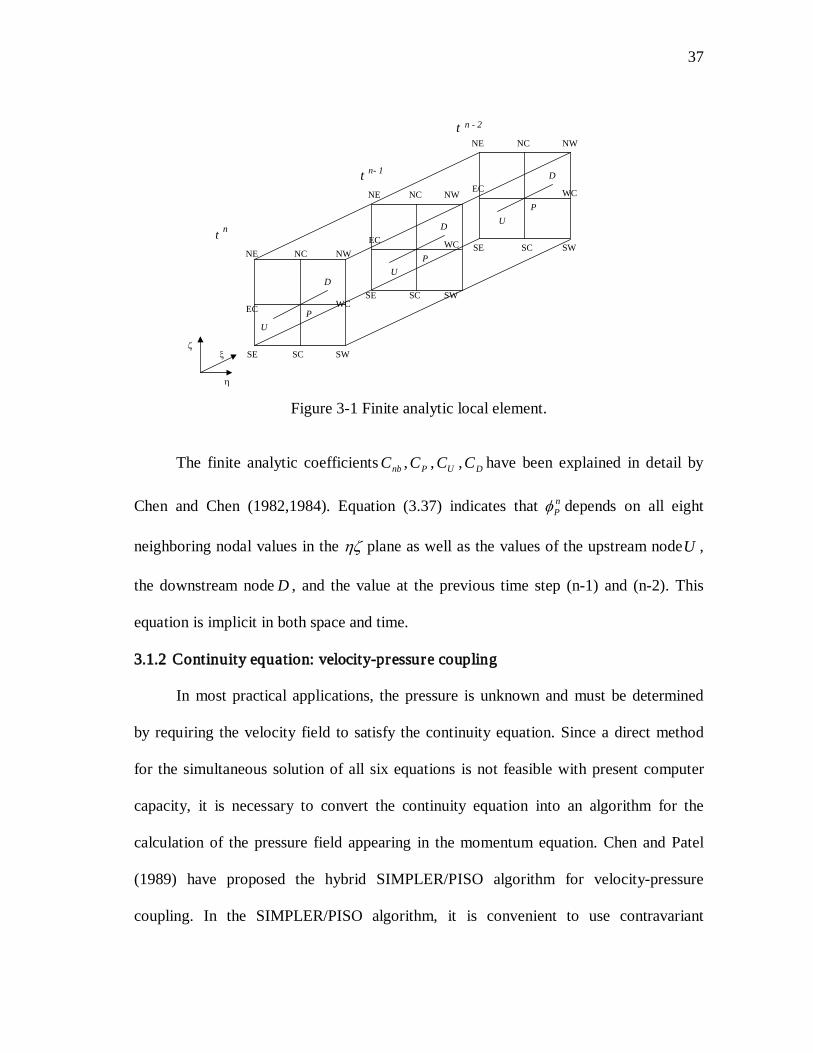
37
NE NC NW
WC
SW SC SE
EC P
D
NE NC NW
EC WC
SW SE SC
P
D
U
U
t n- 1
t
η
ζ ξ
t n - 2
NE NC NW
EC WC
SW SE SC
P
D
U
n
Figure 3-1 Finite analytic local element.
The finite analytic coefficients nbC , PC , UC , DC have been explained in detail by
Chen and Chen (1982,1984). Equation (3.37) indicates that nPφ depends on all eight
neighboring nodal values in the ηζ plane as well as the values of the upstream nodeU ,
the downstream node D , and the value at the previous time step (n-1) and (n-2). This
equation is implicit in both space and time.
3.1.2 Continuity equation: velocity-pressure coupling
In most practical applications, the pressure is unknown and must be determined
by requiring the velocity field to satisfy the continuity equation. Since a direct method
for the simultaneous solution of all six equations is not feasible with present computer
capacity, it is necessary to convert the continuity equation into an algorithm for the
calculation of the pressure field appearing in the momentum equation. Chen and Patel
(1989) have proposed the hybrid SIMPLER/PISO algorithm for velocity-pressure
coupling. In the SIMPLER/PISO algorithm, it is convenient to use contravariant

38
components ( )321 ,, UUU of the velocity vector in the body-fitted
coordinates ( )τξξξ ,,, 321 . Hence, the continuity equation can be expressed as:
∑=
=∂∂3
10
ii
iUξ
(3.38)
Furthermore, the contravariant components of the velocity vector can be specified
into a pressure dependent term and a pseudo-velocity term as below:
iiiii pEUU
ξ∂∂
−= ˆ (3.39)
where
∑=
∂−
∂∂
−=3
1
ˆˆn
kik
jijni
ni pEpEUbU
ξξ (3.40)
( )[ ]∑=∆+++=
3
1/5.11 m
jm
im
DUp
pij bbRCCCJ
CRE
τφ
φ (3.41)
A relationship for pressure can now be derived by requiring the contravariant
velocity field, iU , to satisfy the equation of continuity. An approximating equation
(3.38) with central differences and substituting equation (3.39) for each point in the
stencil gives:
( )
DPEPEPEPEPEPE
PEEEEEE
WCwECeSCsNCnUuDd
pwesnud
ˆ333322221111
333322221111
−+++++=
+++++ (3.42)
where
( )332211
332211
ˆˆˆˆˆˆ21
ˆˆˆˆˆˆˆ
WCECSCNCUD
wesnud
UUUUUU
UUUUUUD
−+−+−=
−+−+−= (3.43)
39
3.2 Boundary Conditions
Boundary conditions described the interface between surroundings and the system
that is modeled. The boundary conditions for the system can be classified into no-slip
boundary, inlet boundary, outlet boundary and free surface boundary conditions.
3.2.1 No slip boundary condition
At the abutment surface or riverbed surface apply the no slip boundary for all
directions, i.e.:
0=iU (3.44)
Extrapolation points near the solid boundary are used to determine the pressure at
the solid boundary surface.
0=∂∂np
(3.45)
3.2.2 Outlet boundary condition
In the viscous flow, a zero gradient boundary condition is used at the far field,
which can be expressed as:
0=∂∂
=∂∂
np
nU i (3.46)
3.2.3 Inlet boundary condition
On the inlet, the velocity and the pressure are prescribed. It is assumed:
0,1 321 ==== pUUU (3.47)

40
3.2.4 Free surface boundary condition
The free surface elevation δ is a function of two other space directions and time,
i.e., ( )tyxzz surf ,,δδ =−= , surfz is the initial water surface elevation taken as the
datum for the hydrostatic force. Based on the chain rule, the kinematics boundary
conditions on the free surface are expressed as:
y
Ux
Utdt
dU∂∂
+∂∂
+∂∂
==δδδδ
213 (3.48)
Equation (3.48) ensures the fluid particles on the free surface remain on the free
surface and it can be solved by simply extrapolating the velocities from the inner fluid
domain. For open channel problem, gravity plays the important role, which has not been
included in the momentum equation (3.2). By ignoring the surface tension and free
surface turbulent boundary layer, the effect of the gravity could be considered in the
pressure term. Conservation of momentum of a viscous fluid flow with a gravitational
acceleration in the vertical direction can be written as:
0Re1
232
3
1=+∇−
∂∂
+
∂
∂+
∂∂
+∂∂ ∑
= FrU
xp
xuu
xU
Ut
U ii
ij j
ji
j
ij
i δ (3.49)
Fr is the Froude number,gB
UFr 0= , where g is the gravitational acceleration.
By introducing a new variable for the pressure, which includes both of the
hydrostatic and static component of the pressure 23
Frx
p +=ψ , the equation of the
momentum can be rewritten as:

41
0Re1 2
3
1=∇−
∂∂
+
∂
∂+
∂∂
+∂∂ ∑
=i
ij j
ji
j
ij
i Uxx
uuxU
Ut
U ψ (3.50)
The Froude number will now enter explicitly in the boundary condition instead of
the governing equation. The procedure mentioned in the previous section can still be
used to solve the open channel flow with the suitable boundary condition applied.
A dynamic condition has also to be fulfilled at the surface. If the surface tension is
neglected and the flow is considered non viscous on the surface, the dynamic boundary
conditions can be simplified to be atmpp = , atmp is the atmospheric pressure. The
corresponding boundary condition for ψ becomes
2Frpatm
δψ += (3.51)
If we say 0=atmp , then
2Frδψ = (3.52)
3.3 Clear Water Scour
Clear water scour means the effect of the deposition can be ignored. Once the soil
eroded, it is eroded. Basically, clear water scour appears on the cohesive riverbed. For
cohesive soil, it is known that the scour rate, defined as the change of scour depth per
unit time, mainly depends on the shear stress at the streambed surface. The initiation of
the scour process is determined by the critical shear stress, the smallest streambed shear
stress to start the erosion process. Based on this understanding, the scour rate can be

42
expressed as a function of the streambed shear stress and the critical shear stress. The
scour rate equation can be written in the following dimensional form:
( )cbzz ττ , = (3.53)
where z is the scour rate, bτ is the streambed shear stress, and cτ is the critical shear
stress. The bτ is evaluated using the Newtonian stress-strain law:
*n
b zq
∂∂
= ρντ (3.54)
where q is the magnitude of flow velocity, *nz is the normal distance from the streambed.
In numerical computation, after the flow field is computed at each time step, the scour
rate at each point is determined by the scour rate equation. The increase of scour depth is
then evaluated by multiplying the scour rate by the time increment.
3.4 Overall Solution Algorithm
For the scour problem involving the grid movement on the river bed and free
surface variation, the solution procedure can be summarized as follows:
1. Construct the grid for each component of the configuration.
2. Construct a boundary condition table specifying appropriate boundary
conditions for each face.
3. Specify the initial condition for velocity, pressure, and turbulence fields.
4. Determine interpolation information to link the grids together using the
PEGSUS program.
5. Calculate the geometric coefficients.
6. Calculate the finite analytic coefficients and source functions.

43
7. Solve the momentum equations ( )iU and turbulence equations ( )ε,k using the
iterative ADI scheme.
8. Calculate the pseudo velocities ( )iV and calculate pressure ( )p using the
iterative ADI scheme.
9. Repeat step 7 and 8.
10. Calculate the new free surface elevation using kinematics free surface
boundary conditions.
11. For clear water scour, calculate the new bed surface elevation using the
scour rate equation.
12. Adjust the volume grid to conform to free surface and riverbed elevations in
z-direction.
13. Return to step 4 for next time step.

44
CHAPTER IV
MAXIMUM BED SHEAR STRESS
AROUND ABUTMENT IN OPEN CHANNEL FLOW
The maximum bed shear stress around abutment, one of the two basic parameters
in SRICOS method, is studied in this chapter. All the simulation results given in this
chapter are with open channel flow. The maximum bed shear stress around abutment is
studied first on the simple rectangular channel. After the establishment of the maximum
bed shear stress equation on rectangular channel, compound channel correction factor is
further proposed so that the equation can be extended to include compound channel
situations. CHEN3D program introduced in chapter III is utilized to achieve all the
numerical simulations. The flume test cases of NCHRP 24-15(2) are simulated
numerically and used to verify the proposed equation. Finally, the apparent maximum
bed shear stress around abutment is recommended based on the results of flume tests and
the erosion function of the soils from EFA testing.
4.1 Methodology
The typical river channel including abutment and approach embankment is
presented in figure 4-1. In the real world, the elevation of river bed may change
gradually from the center of main channel to flood plain and have no clear main channel
slope as shown in the diagram. Main channel slope mβ may vary in a large range,
depending on the soil type, from a small number in sands to even vertical in cohesive
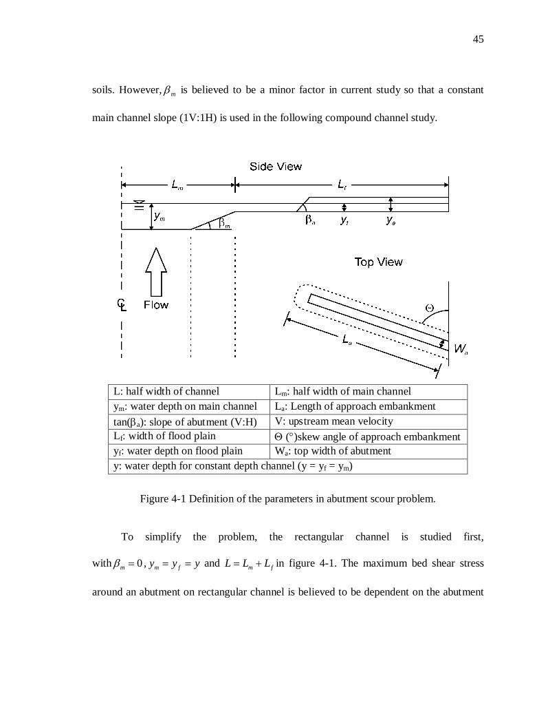
45
soils. However, mβ is believed to be a minor factor in current study so that a constant
main channel slope (1V:1H) is used in the following compound channel study.
Figure 4-1 Definition of the parameters in abutment scour problem.
To simplify the problem, the rectangular channel is studied first,
with 0mβ = , m fy y y= = and m fL L L= + in figure 4-1. The maximum bed shear stress
around an abutment on rectangular channel is believed to be dependent on the abutment
L: half width of channel Lm: half width of main channel ym: water depth on main channel La: Length of approach embankment tan(βa): slope of abutment (V:H) V: upstream mean velocity Lf: width of flood plain Θ (°)skew angle of approach embankment yf: water depth on flood plain Wa: top width of abutment y: water depth for constant depth channel (y = yf = ym)
46
geometry, channel width, water depth, approach velocity, water density, fluid viscosity
and gravitational acceleration. The relationship can be sought in the form:
[ ]max , , , , , , , , ,a a af V y g L L Wτ ρ ν β= Θ (4-1)
Where maxτ = maximum bed shear stress around abutment, ρ = water density,
V = upstream mean velocity, ν = kinematic viscosity of the fluid , y = upstream water
depth, g = gravitational acceleration, aL = length of abutment and the approach
embankment(to the toe of the abutment), L = half width of the channel, aW = top width
of the abutment, aβ = slope of the abutment, and Θ = skew angle of approach
embankment. For convenience, aL is defined as the projected length normal to the flow
in the flowing study.
Dimensional analysis of the equation (4-1) results in:
max2 , , , , , ,a a a
aa a
VW L LV yfV W L Wgy
τ βρ ν
= Θ
(4-2)
It is desirable to use the top width of the abutment aW as the characteristic length
because aW is typically fixed for a given bridge (same to the width of bridge deck).
Re aVWν
= is the abutment size based Reynolds number; Vgy
is the upstream Froude
number; a
a
LW
is the aspect ratio of the abutment and approach embankment; aLL
is the
blockage ratio; a
yW
is the relative flow depth. For rectangular channel, the upstream

47
mean velocity could be assumed to be uniform across the entire channel. So the channel
contraction ratio rC defined by flow rate at upstream total
total blocked
QQ Q−
is identical to the
area ratio total
total blocked
AA A−
. It is also worthwhile to note that rC is equal to a
LL L−
for the
vertical wall and wing-wall abutments. For convenience, rC based on the area ratio
total
total blocked
AA A−
will be used to replace the blockage ratio in the dimensional analysis in the
following study.
The methodology includes the determination of reference case and the parametric
studies of the dimensionless parameters given in dimensional analysis. According to the
previous study (Briaud et al. 1999, 2003), it is believed that Reynolds number is the
determinant factor on maximum bed shear stress around abutment when the relative
water depth is greater than two. Hence, the reference case is designed for the
convenience of Reynolds study while other correction factors are taken as one. In
parametric studies, only one dimensionless parameter is varied and all the others are kept
identical to the reference case. The relationship between the varied dimensionless
parameter and the maximum bed shear stress can then be determined through data
regression. By assuming that these dimensionless parameters are independent, the
equation of maximum bed shear stress around abutment on rectangular channel can be
derived by timing them together. The influence of compound channel geometry will be
investigated by comparing the results of a series cases simulated with different
compound channel configuration.
48
4.2 Reference Case
The flow pattern at an abutment is considered to be similar to that around a pier of
shape equivalent to the abutment and its mirror image with respect to the channel wall.
The maximum bed shear stress at the abutment, however, should be less than that around
the equivalent pier due to the retarding effects of channel wall on the flow (Melville,
1997). Based on previous research (NCHRP 24-15, Briaud et al., 2003), the influence of
water depth on maximum bed shear stress around bridge pier can be ignored when water
depth is deeper than two times of pier diameter, which is called deep water condition.
Actually, this indicates the influence of Froude number is negligible as long as the
relative flow depth is large enough. Therefore, it is convenient to define the reference
case as a vertical wall abutment in a rectangular channel as shown in Figure 4-2. The
abutment length is chosen to be one-half of the abutment width such that the abutment
together with its mirror image forms a square pier. The orientation of the abutment is
perpendicular to the flow direction and the water depth is twice of the abutment width to
ensure that the influence of Froude number is negligible. Hence, the detailed dimensions
of the reference case can be determined according to the flume tests in NCHRP 24-15(2).
The width of the flume employed is 12ft, which is equal to the half width of the channel
L since only half of the river is simulated in flume tests. And the top width of the
abutment aW is 1.5 ft. So the water depth is 3ft. As seen in Figure 4-2, the half width of
the channel L is 8 times of the abutment width aW , which gives a rather small
contraction ratio of 1.07 (blockage ratio of 6.25%).
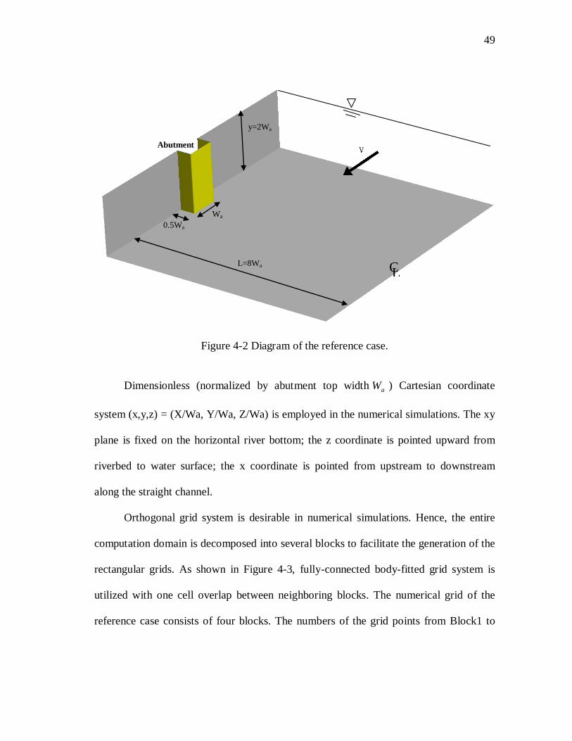
49
Figure 4-2 Diagram of the reference case.
Dimensionless (normalized by abutment top width aW ) Cartesian coordinate
system (x,y,z) = (X/Wa, Y/Wa, Z/Wa) is employed in the numerical simulations. The xy
plane is fixed on the horizontal river bottom; the z coordinate is pointed upward from
riverbed to water surface; the x coordinate is pointed from upstream to downstream
along the straight channel.
Orthogonal grid system is desirable in numerical simulations. Hence, the entire
computation domain is decomposed into several blocks to facilitate the generation of the
rectangular grids. As shown in Figure 4-3, fully-connected body-fitted grid system is
utilized with one cell overlap between neighboring blocks. The numerical grid of the
reference case consists of four blocks. The numbers of the grid points from Block1 to
Wa 0.5Wa
y=2Wa
L=8Wa
Abutment
C L
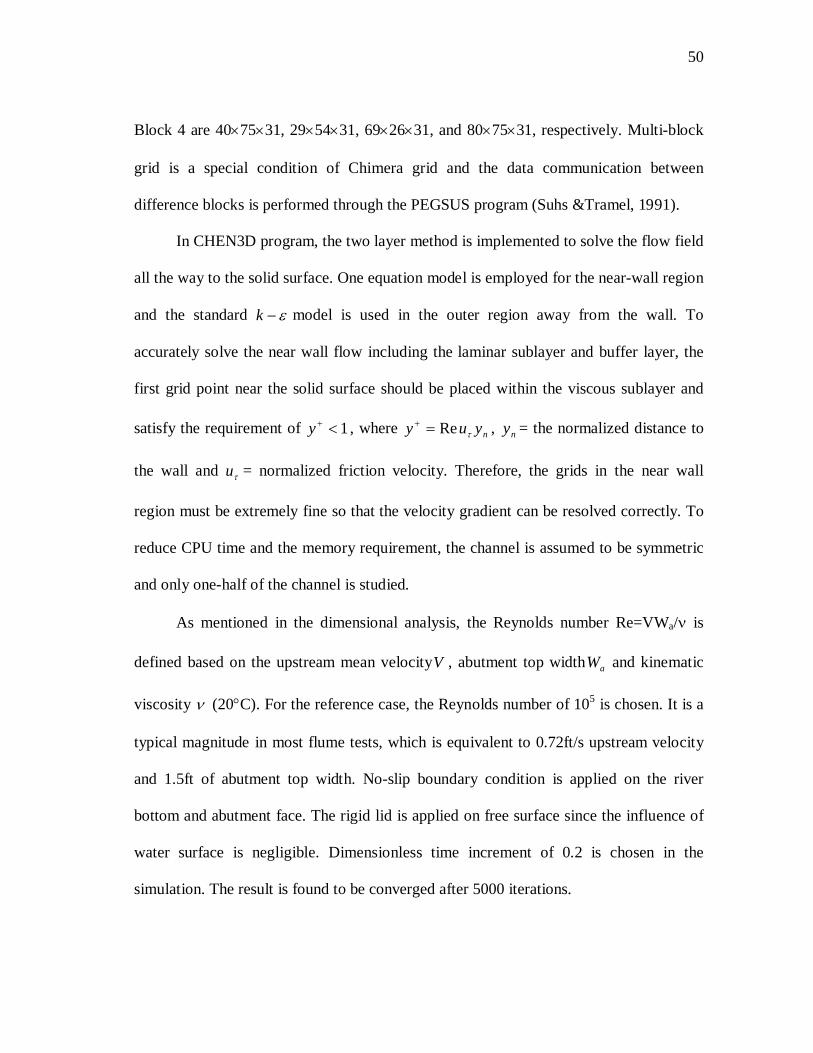
50
Block 4 are 40×75×31, 29×54×31, 69×26×31, and 80×75×31, respectively. Multi-block
grid is a special condition of Chimera grid and the data communication between
difference blocks is performed through the PEGSUS program (Suhs &Tramel, 1991).
In CHEN3D program, the two layer method is implemented to solve the flow field
all the way to the solid surface. One equation model is employed for the near-wall region
and the standard ε−k model is used in the outer region away from the wall. To
accurately solve the near wall flow including the laminar sublayer and buffer layer, the
first grid point near the solid surface should be placed within the viscous sublayer and
satisfy the requirement of 1<+y , where nyuy τRe=+ , ny = the normalized distance to
the wall and τu = normalized friction velocity. Therefore, the grids in the near wall
region must be extremely fine so that the velocity gradient can be resolved correctly. To
reduce CPU time and the memory requirement, the channel is assumed to be symmetric
and only one-half of the channel is studied.
As mentioned in the dimensional analysis, the Reynolds number Re=VWa/ν is
defined based on the upstream mean velocityV , abutment top width aW and kinematic
viscosity ν (20°C). For the reference case, the Reynolds number of 105 is chosen. It is a
typical magnitude in most flume tests, which is equivalent to 0.72ft/s upstream velocity
and 1.5ft of abutment top width. No-slip boundary condition is applied on the river
bottom and abutment face. The rigid lid is applied on free surface since the influence of
water surface is negligible. Dimensionless time increment of 0.2 is chosen in the
simulation. The result is found to be converged after 5000 iterations.

51
X/Wa
Y/W
a
-1 -0.5 0 0.5 1
0.5
1
1.5
Abutment
Block1 Block2 Block3 Block4
Figure 4-3 Numerical grid for the reference case.
52
X/Wa
Y/W
a
-1 -0.5 0 0.5 1
0.5
1
1.5
1
Figure 4-4 Velocity vectors on water surface (reference case).
Figure 4-4 shows the flow pattern around abutment on the free surface. The
abutment causes complicated flow features, including vortex shedding, wake vortices
and large recirculation behind the abutment. At upstream of the abutment, the affected
area is very small, about one time of abutment length. At the downstream of the
abutment, the affected area is very large. The area of the recirculation can be as large as
several times of abutment length. This large recirculation continues to congest the flow
and force the flow moving toward channel center. This is why the velocity magnitude is
higher at the downstream instead of middle of the abutment along the channel center. At
the upstream corner of the abutment, the flow is mostly accelerated and forced around
53
the abutment. The maximum velocity appears around the upstream corner. However,
only in the region very adjacent to the abutment, the velocity increased significantly. In
the transverse direction, the flow is disturbed seriously only in a narrow range in front of
the abutment face. Outside of that range, the velocity vectors remain uniform. The
influence can only be reflected from the flow direction and the velocity magnitude. The
flow separation appears right on the abutment face.
Figure 4-5 shows the normalized pressure contours around abutment. At the
upstream side, the higher pressure occurs due to the obstacle of the abutment. Pressure
drops sharply at the upstream corner; this is consistent with the local velocity
acceleration. The pressure recovers the uniform distribution very quickly away from the
abutment.
Figure 4-6 presents the bed shear stress distribution. The maximum bed shear
stress is about 0.5 Pa at the upstream corner of the abutment. This is the initial bed shear
stress contour before scouring. The shear stress will continue to decrease with the
development of the scour hole. The scour process stops when the bed shear stress
reaches the critical shear stress of the bed soils.
To study the influence of the water surface boundary condition, the same cases
with rigid lid and free surface boundary conditions have been simulated. The results
show little influence of surface boundary to the maximum bed shear stress around
abutment. The difference is within 2%. And for most of cases in actual engineering
application, the blockage of the river will not be very large. Hence this assumption
should be reasonable.

54
Figure 4-5 Normalized pressure contours around vertical wall abutment.
0.200.40
0.60
1.00
0.34 0.28
0.10
X/Wa
Y/W
a
-0.5 0 0.50
0.5
1 Flow
Abutment
Figure 4-6 Bed friction coefficient (×10-2) contour for Reynolds number 105.
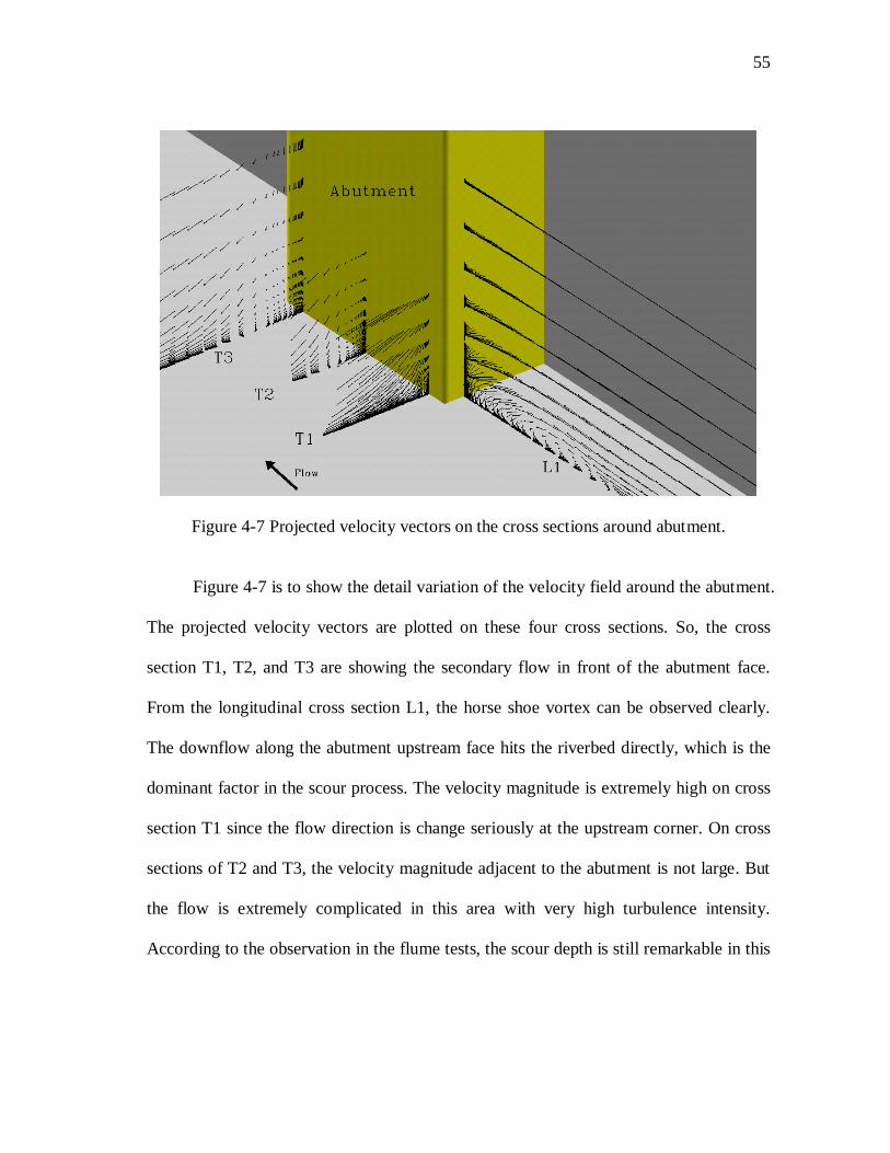
55
Figure 4-7 Projected velocity vectors on the cross sections around abutment.
Figure 4-7 is to show the detail variation of the velocity field around the abutment.
The projected velocity vectors are plotted on these four cross sections. So, the cross
section T1, T2, and T3 are showing the secondary flow in front of the abutment face.
From the longitudinal cross section L1, the horse shoe vortex can be observed clearly.
The downflow along the abutment upstream face hits the riverbed directly, which is the
dominant factor in the scour process. The velocity magnitude is extremely high on cross
section T1 since the flow direction is change seriously at the upstream corner. On cross
sections of T2 and T3, the velocity magnitude adjacent to the abutment is not large. But
the flow is extremely complicated in this area with very high turbulence intensity.
According to the observation in the flume tests, the scour depth is still remarkable in this
56
area. This implies that both the velocity magnitude and the turbulence intensity can
contribute to the scour development.
4.3 Parametric Studies
4.3.1 Influence of Reynolds number
For the pier study in NCHRP 24-15 (Briaud et al., 2003), half of the domain was
computed with the symmetric line passing the center of circular pier. The symmetric
boundary condition was applied on both the symmetric line and the other side away from
the pier. In current study, symmetric assumption is also adopted and the symmetric line
is along the center of the channel. No-slip boundary is applied on the side wall with
abutment. So, the only difference between the previous pier study and the current
abutment study is the boundary condition along with the hydraulic structures. To
investigate the influence of the boundary conditions, the same grid has been tested for
these two settings of pier and abutment (half of the circular pier). And the maximum bed
shear stress around the abutment is about 2/3 of that around pier. This indicates that the
influence of Reynolds number on the maximum bed shear stress around abutment is not
identical to the proposed pier equation in previous report of NCHRP 24-15. Hence, there
is a need to study the influence of Reynolds number on the maximum bed shear stress
around the abutment. Another reason is that the typical abutment shape is vertical wall
instead of circular cylinder. The influence of shape could be significant.
As discussed before, the maximum bed shear stress is believed to be the function
of Reynolds number. The influence of Froude number is negligible as long as the
relative flow depth is large enough. Further assuming the correction factors from all the
57
other dimensionless parameters are one for the reference case. The equation (4-2) can be
further simplified as,
=νρ
τ aVWf
V 2max (4-3)
Numerical simulations were conducted for eight different Reynolds numbers
(Re=VWa/ν) of 1×10⁴, 2×10⁴, 5×10⁴, 1×10⁵, 5×10⁵, 1×10⁶, 5×10⁶ and 1×10⁷ based on the
same geometry as the reference case. Figure 4-8 shows the variation of the computed
maximum bed friction coefficient (Cf_vw) around vertical wall abutment with Reynolds
number. For completeness, the maximum bed friction coefficient Cf_cp equation for
circular pier by Briaud et al. (1999) is also shown in the same figure. Both curves show
that the normalized maximum bed shear stress decreases with the increase of Reynolds
number. It should be noted that this does not mean that the dimensional bed shear stress
also decreases with Reynolds number because it depends on not only Reynolds number
but also the upstream velocity. The discrepancy, shown in figure 4-8, between the
previous pier study and current abutment study is from both the hydraulic structure
shape and the side boundary conditions. Generally, the bed shear stress is higher around
vertical wall abutment than around circular pier. The separation point around vertical
abutment is always at the sharp upstream corner in spite of the magnitude of the
Reynolds number. While the separation point around circular pier is changing with
Reynolds number. In figure 4-8, the curve for circular pier is much flatter than the one
for vertical wall. Cf_vw is higher than Cf_cp when Reynolds number is smaller than 3×10⁵.
When the Reynolds number is higher than 3×10⁵, the curve for vertical wall also tends to

58
be flat and the magnitude is lower than that for circular pier. There is one possibility that
the influence from the boundary may also vary with the Reynolds number. According to
the simulation results, the equation for circular pier is not suitable for the abutment
analysis. Another interesting observation is that the difference between these two curves
tends to be small when Reynolds number is very high. As show in Fig 4-8, these two
curves are almost parallel in the high Reynolds region. Figures 4-9, 4-10, and 4-11
present the simulated bed friction coefficient contours for different Reynolds numbers.
Figure 4-8 Normalized maximum bed shear stresses versus Reynolds number.

59
1.50
3.003.00
1.00
0.70
0.50
0.19
0.03
X/Wa
Y/W
a
-0.5 0 0.50
0.5
1 Flow
Abutment
Figure 4-9 Bed friction coefficient (×10-2) contour for Reynolds number 104.
0.10
0.20
0.30
0.40
0.02
0.26
X/Wa
Y/W
a
-0.5 0 0.50
0.5
1 Flow
Abutment
Figure 4-10 Bed friction coefficient (×10-2) contour for Reynolds number 106.
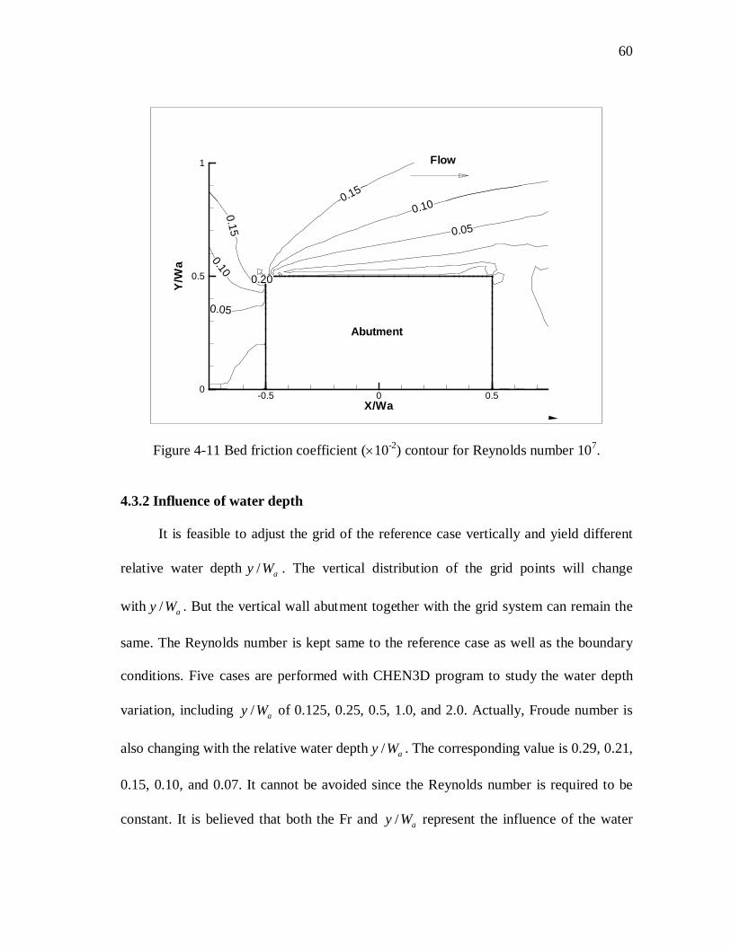
60
0.05
0.100.15
0.20
0.150.10
0.05
X/Wa
Y/W
a
-0.5 0 0.50
0.5
1 Flow
Abutment
Figure 4-11 Bed friction coefficient (×10-2) contour for Reynolds number 107.
4.3.2 Influence of water depth
It is feasible to adjust the grid of the reference case vertically and yield different
relative water depth / ay W . The vertical distribution of the grid points will change
with / ay W . But the vertical wall abutment together with the grid system can remain the
same. The Reynolds number is kept same to the reference case as well as the boundary
conditions. Five cases are performed with CHEN3D program to study the water depth
variation, including / ay W of 0.125, 0.25, 0.5, 1.0, and 2.0. Actually, Froude number is
also changing with the relative water depth / ay W . The corresponding value is 0.29, 0.21,
0.15, 0.10, and 0.07. It cannot be avoided since the Reynolds number is required to be
constant. It is believed that both the Fr and / ay W represent the influence of the water

61
depth on maxτ around the abutment. So Froude number is used to in the data regression.
One way to present the result is to plot max max_/ referenceτ τ as a function of Fr. The shallow
water correction factor, wK , is the ratio of max max_/ referenceτ τ . Figure 4-12 presents the
results of the five simulations. When the Froude number is smaller than 0.10, the
influence of the water depth is negligible. Figures 4-13, 4-14, and 4-15 show the results
of friction coefficient contours of different water depth. Water depth variation has little
influence on the bed shear stresses away from the abutment.
0.0
0.5
1.0
1.5
2.0
0.0 0.1 0.2 0.3 0.4
F r=V *(gy) -̂0.5
KF
r
K F r = 2.07F r+0.8
Figure 4-12 Correction factor for water depth.
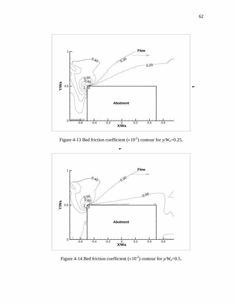
62
1.40
0.60
0.200.300.40
0.50
X/Wa
Y/W
a
-0.6 -0.4 -0.2 0 0.2 0.4 0.60
0.5
1 Flow
Abutment
Figure 4-13 Bed friction coefficient (×10-2) contour for y/Wa=0.25.
1.20
0.600.06
0.300.40
0.50
X/Wa
Y/W
a
-0.6 -0.4 -0.2 0 0.2 0.4 0.60
0.5
1 Flow
Abutment
Figure 4-14 Bed friction coefficient (×10-2) contour for y/Wa=0.5.

63
1.10
0.600.06
0.300.40
0.50
X/Wa
Y/W
a
-0.6 -0.4 -0.2 0 0.2 0.4 0.60
0.5
1 Flow
Abutment
Figure 4-15 Bed friction coefficient (×10-2) contour for y/Wa=1.0.
4.3.3 Influence of channel contraction ratio
The objective of this parametric study is to obtain the relationship between the
maximum bed shear stress maxτ and the channel contraction ratio rC . The grid of
reference case is modified to have L equal to 0.83 aW , 1.25 aW , and 2.5 aW . All other
parameters remain same as the reference case. Figure 4-16 presents the variation of the
channel width. Figures 4-18, 4-19, and 4-20 show the contours of the normalized bed
shear stress contours for different contraction ratios. The velocity and the bed shear
stress increase with the increase of contraction ratio. The maximum bed shear stress maxτ
is the maximum shear stress that exists on the river bed just before the scour hole to
develop. One way to present the data is to plot max max_/ referenceτ τ as a function of

64
contraction ratio rC shown in figure 4-17. The contraction ratio correction factor, CrK ,
is the ratio of max max_/ referenceτ τ . The data points on figure 4-17 correspond to the results
of the three simulations and the reference case. By data regression, the correction factor
CrK is found to be linear proportional with the contraction ratio rC . Higher contraction
ratio means that the channel is highly blocked. It should be noted that the contraction
ratio rC for the reference case is 1.07 and the corresponding correction factor CrK is
equal to 1.0. For the limiting case of a very wide channel with rC → 1, it is anticipated
that the maximum shear stress around the abutment will be approximately 20% lower
(i.e., CrK = 0.8) than the corresponding value for the reference case.
Figure 4-16 Geometries for channel contraction ratio study.
Wa La=0.5Wa
y=2Wa
L=8Wa
Abutment
L=2.5Wa
L=1.25Wa L=0.83Wa

65
0.0
2.0
4.0
6.0
8.0
1.0 1.5 2.0 2.5 3.0
C ontraction R atio, C r
KC
r
Figure 4-17 Correction factor for channel contraction ratio.
7.201.00
2.00
3.00
3.002.
00
1.00
3.50
0.50
0.50
X/Wa
Y/W
a
-0.2 0 0.2 0.4 0.6 0.8 1 1.20
0.5
1 Flow
Abutment
Figure 4-18 Bed friction coefficient (×10-2) contour for rC =0.4.
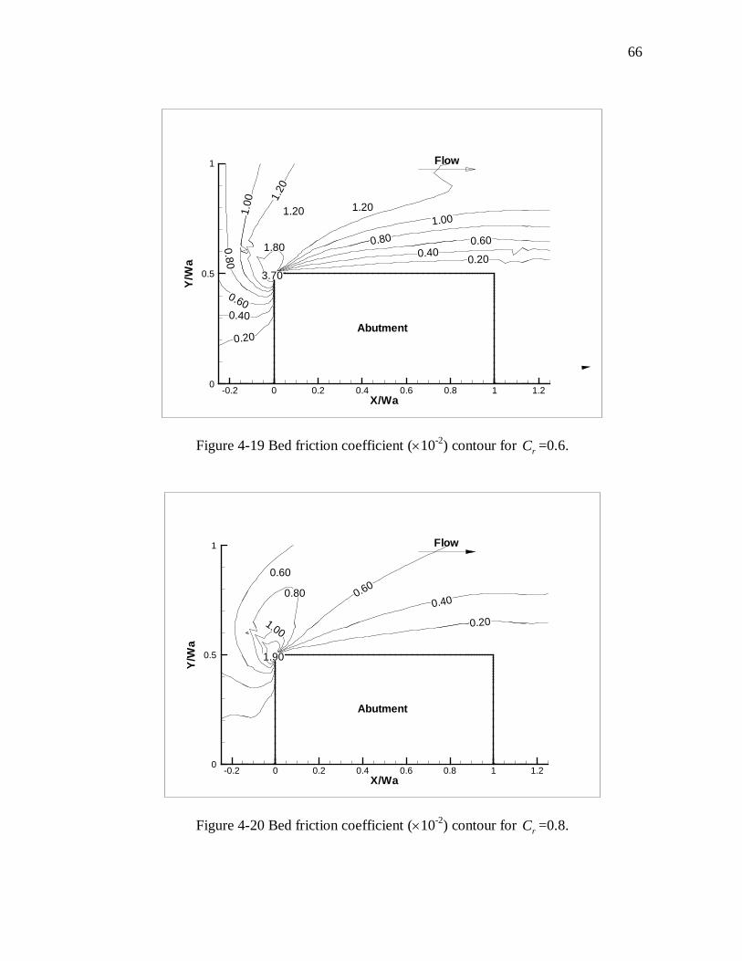
66
1.20
1.20
0.60
1.001.20
1.80
3.700.200.40
0.801.
00
0.80
0.600.40
0.20
X/Wa
Y/W
a
-0.2 0 0.2 0.4 0.6 0.8 1 1.20
0.5
1 Flow
Abutment
Figure 4-19 Bed friction coefficient (×10-2) contour for rC =0.6.
0.600.60
0.20
0.400.80
1.00
1.90
X/Wa
Y/W
a
-0.2 0 0.2 0.4 0.6 0.8 1 1.20
0.5
1 Flow
Abutment
Figure 4-20 Bed friction coefficient (×10-2) contour for rC =0.8.
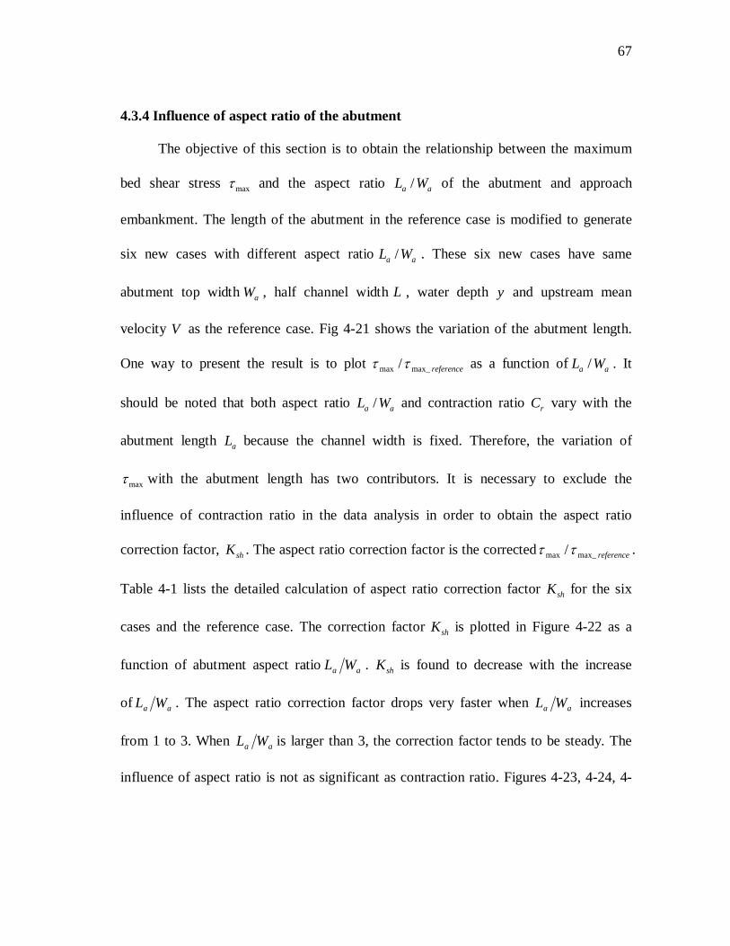
67
4.3.4 Influence of aspect ratio of the abutment
The objective of this section is to obtain the relationship between the maximum
bed shear stress maxτ and the aspect ratio /a aL W of the abutment and approach
embankment. The length of the abutment in the reference case is modified to generate
six new cases with different aspect ratio /a aL W . These six new cases have same
abutment top width aW , half channel width L , water depth y and upstream mean
velocity V as the reference case. Fig 4-21 shows the variation of the abutment length.
One way to present the result is to plot referencemax_max /ττ as a function of /a aL W . It
should be noted that both aspect ratio /a aL W and contraction ratio rC vary with the
abutment length aL because the channel width is fixed. Therefore, the variation of
maxτ with the abutment length has two contributors. It is necessary to exclude the
influence of contraction ratio in the data analysis in order to obtain the aspect ratio
correction factor, shK . The aspect ratio correction factor is the corrected referencemax_max /ττ .
Table 4-1 lists the detailed calculation of aspect ratio correction factor shK for the six
cases and the reference case. The correction factor shK is plotted in Figure 4-22 as a
function of abutment aspect ratio aa WL . shK is found to decrease with the increase
of aa WL . The aspect ratio correction factor drops very faster when aa WL increases
from 1 to 3. When aa WL is larger than 3, the correction factor tends to be steady. The
influence of aspect ratio is not as significant as contraction ratio. Figures 4-23, 4-24, 4-
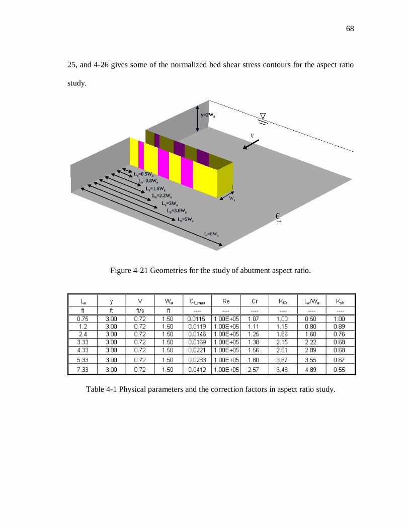
68
25, and 4-26 gives some of the normalized bed shear stress contours for the aspect ratio
study.
Wa
La=5Wa
La=3.6Wa
La=3Wa
La=2.2Wa
La=1.6Wa
La=0.8Wa
La=0.5Wa
y=2Wa
L=8Wa
Wa
La=5Wa
La=3.6Wa
La=3Wa
La=2.2Wa
La=1.6Wa
La=0.8Wa
La=0.5Wa
La=5Wa
La=3.6Wa
La=3Wa
La=2.2Wa
La=1.6Wa
La=0.8Wa
La=0.5Wa
y=2Way=2Wa
L=8Wa
Figure 4-21 Geometries for the study of abutment aspect ratio.
Table 4-1 Physical parameters and the correction factors in aspect ratio study.
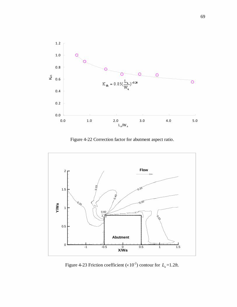
69
0.0
0.2
0.4
0.6
0.8
1.0
1.2
0.0 1.0 2.0 3.0 4.0 5.0L a/W a
K sh
Figure 4-22 Correction factor for abutment aspect ratio.
1.15
0.20
0.40
0.60
0.33
0.20
0.33
0.02
X/Wa
Y/W
a
-1 -0.5 0 0.5 1 1.50
0.5
1
1.5
2 Flow
Abutment
Figure 4-23 Friction coefficient (×10-2) contour for aL =1.2ft.
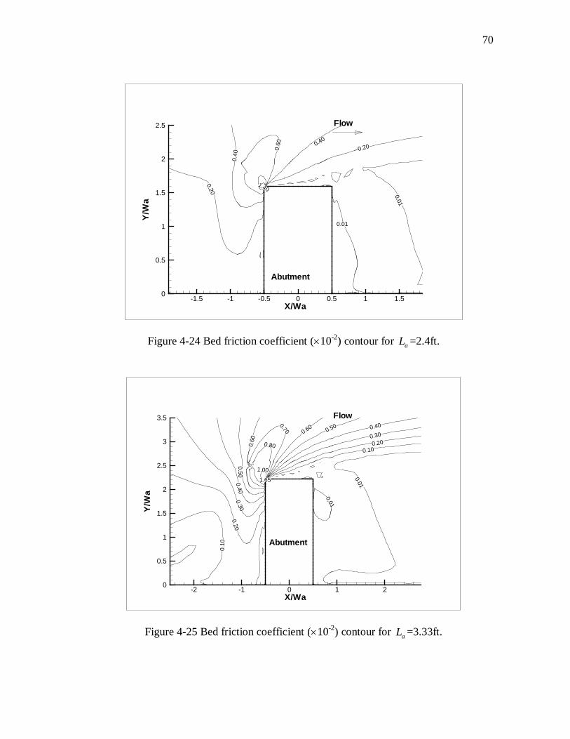
70
0.200.40
0.60
1.40
0.40
0.20 0.01
0.01
X/Wa
Y/W
a
-1.5 -1 -0.5 0 0.5 1 1.50
0.5
1
1.5
2
2.5 Flow
Abutment
Figure 4-24 Bed friction coefficient (×10-2) contour for aL =2.4ft.
1.65 0.01
0.100.20
0.300.40
0.500.600.70
0.80
1.00
0.10
0.200.30
0.400.50
0.60
0.01
X/Wa
Y/W
a
-2 -1 0 1 20
0.5
1
1.5
2
2.5
3
3.5 Flow
Abutment
Figure 4-25 Bed friction coefficient (×10-2) contour for aL =3.33ft.
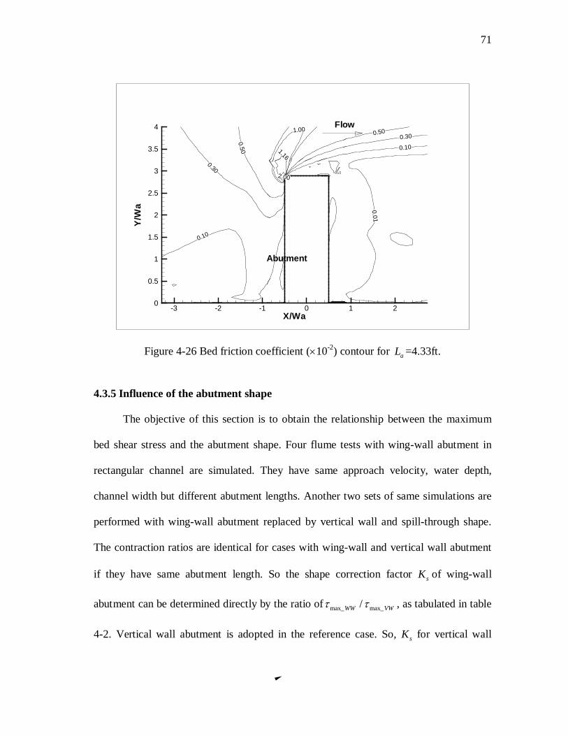
71
2.00
0.01
0.100.300.501.00
1.16
0.50
0.30
0.10
X/Wa
Y/W
a
-3 -2 -1 0 1 20
0.5
1
1.5
2
2.5
3
3.5
4 Flow
Abutment
Figure 4-26 Bed friction coefficient (×10-2) contour for aL =4.33ft.
4.3.5 Influence of the abutment shape
The objective of this section is to obtain the relationship between the maximum
bed shear stress and the abutment shape. Four flume tests with wing-wall abutment in
rectangular channel are simulated. They have same approach velocity, water depth,
channel width but different abutment lengths. Another two sets of same simulations are
performed with wing-wall abutment replaced by vertical wall and spill-through shape.
The contraction ratios are identical for cases with wing-wall and vertical wall abutment
if they have same abutment length. So the shape correction factor sK of wing-wall
abutment can be determined directly by the ratio of max_ max_/WW VWτ τ , as tabulated in table
4-2. Vertical wall abutment is adopted in the reference case. So, sK for vertical wall
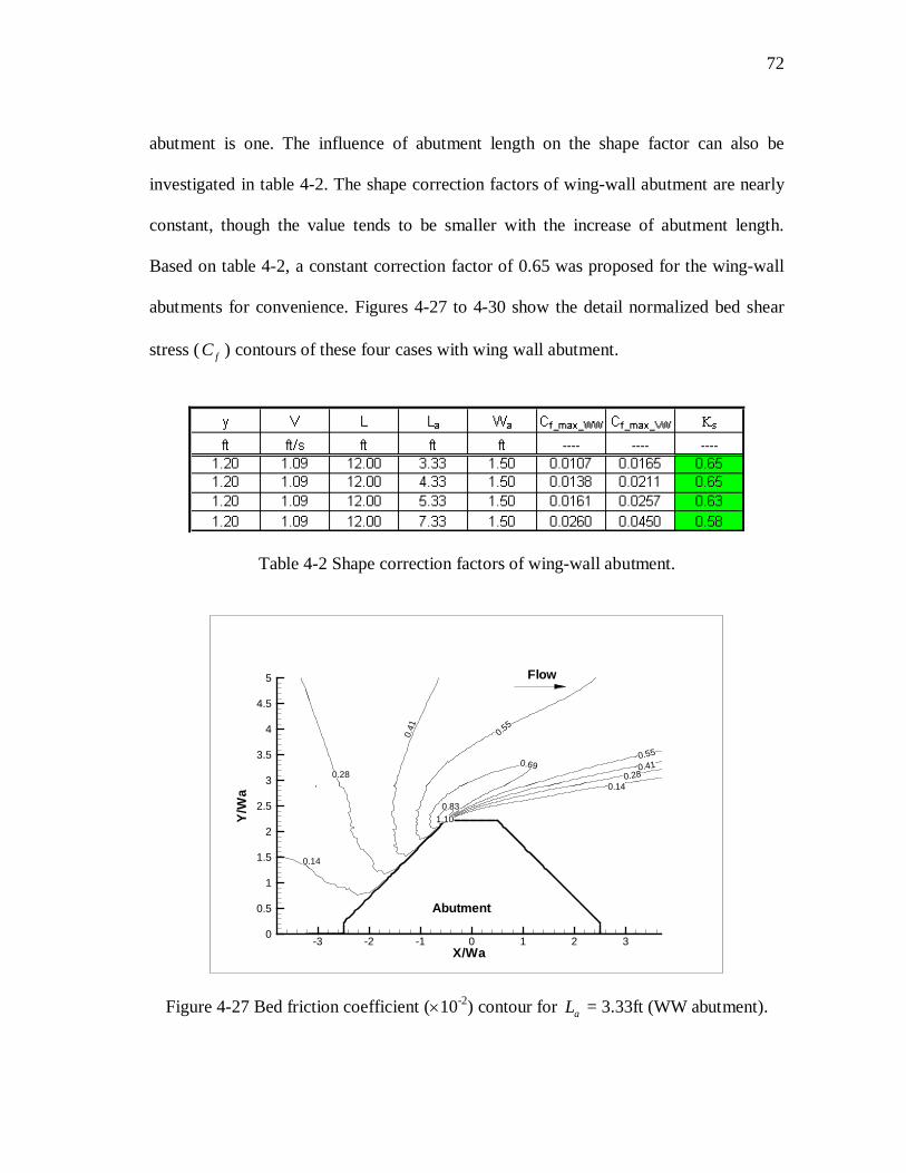
72
abutment is one. The influence of abutment length on the shape factor can also be
investigated in table 4-2. The shape correction factors of wing-wall abutment are nearly
constant, though the value tends to be smaller with the increase of abutment length.
Based on table 4-2, a constant correction factor of 0.65 was proposed for the wing-wall
abutments for convenience. Figures 4-27 to 4-30 show the detail normalized bed shear
stress ( fC ) contours of these four cases with wing wall abutment.
Table 4-2 Shape correction factors of wing-wall abutment.
0.140.28
0.410.55
0.69
0.55
0.41
0.28
0.14
0.831.10
X/Wa
Y/W
a
-3 -2 -1 0 1 2 30
0.5
1
1.5
2
2.5
3
3.5
4
4.5
5 Flow
Abutment
Figure 4-27 Bed friction coefficient (×10-2) contour for aL = 3.33ft (WW abutment).

73
0.80
0.20
0.40
0.60
0.60
1.38
1.00
X/Wa
Y/W
a
-3 -2 -1 0 1 2 30
0.5
1
1.5
2
2.5
3
3.5
4
4.5
5 Flow
Abutment
Figure 4-28 Bed friction coefficient (×10-2) contour for aL = 4.33ft (WW abutment).
1.60
0.40
1.200.60
0.20
X/Wa
Y/W
a
-3 -2 -1 0 1 2 30
0.5
1
1.5
2
2.5
3
3.5
4
4.5
5 Flow
Abutment
Figure 4-29 Bed friction coefficient (×10-2) contour for aL = 5.33 ft (WW abutment).
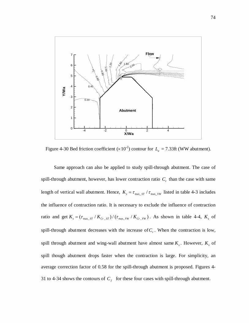
74
2.60
0.20
0.40
0.600.80
1.00
1.20 1.60 1.80
2.00
X/Wa
Y/W
a
-4 -2 0 2 40
1
2
3
4
5
6
7 Flow
Abutment
Figure 4-30 Bed friction coefficient (×10-2) contour for aL = 7.33ft (WW abutment).
Same approach can also be applied to study spill-through abutment. The case of
spill-through abutment, however, has lower contraction ratio rC than the case with same
length of vertical wall abutment. Hence, max_ max_/s ST VWK τ τ= listed in table 4-3 includes
the influence of contraction ratio. It is necessary to exclude the influence of contraction
ratio and get max_ _ max_ _( / ) / ( / )s ST Cr ST VW Cr VWK K Kτ τ= . As shown in table 4-4, sK of
spill-through abutment decreases with the increase of rC . When the contraction is low,
spill through abutment and wing-wall abutment have almost same sK . However, sK of
spill though abutment drops faster when the contraction is large. For simplicity, an
average correction factor of 0.58 for the spill-through abutment is proposed. Figures 4-
31 to 4-34 shows the contours of fC for these four cases with spill-through abutment.
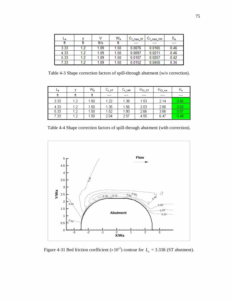
75
Table 4-3 Shape correction factors of spill-through abutment (w/o correction).
Table 4-4 Shape correction factors of spill-through abutment (with correction).
0.100.20
0.30
0.400.500.60
0.30
0.20
0.10
0.700.76
X/Wa
Y/W
a
-3 -2 -1 0 1 2 30
0.5
1
1.5
2
2.5
3
3.5
4
4.5
5 Flow
Abutment
Figure 4-31 Bed friction coefficient (×10-2) contour for aL = 3.33ft (ST abutment).

76
0.97
0.100.200.30
0.400.500.
60
0.50
0.40
0.300.20
0.10
0.700.800.90
X/Wa
Y/W
a
-3 -2 -1 0 1 2 30
0.5
1
1.5
2
2.5
3
3.5
4
4.5
5 Flow
Abutment
Figure 4-32 Bed friction coefficient (×10-2) contour for aL = 4.33ft (ST abutment).
1.07
0.20
0.30
0.40
0.50
0.60
0.800.900.60
0.50
0.400.30 0.20
X/Wa
Y/W
a
-2 0 20
0.5
1
1.5
2
2.5
3
3.5
4
4.5
5 Flow
Abutment
Figure 4-33 Bed friction coefficient (×10-2) contour for aL = 5.33ft (ST abutment).
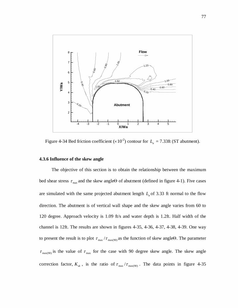
77
1.00
1.52
0.20
0.40
0.60
0.80 1.
00
1.000.80
0.600.40
0.20
1.23
X/Wa
Y/W
a
-4 -3 -2 -1 0 1 2 3 4 5
2
3
4
5
6
7
8 Flow
Abutment
Figure 4-34 Bed friction coefficient (×10-2) contour for aL = 7.33ft (ST abutment).
4.3.6 Influence of the skew angle
The objective of this section is to obtain the relationship between the maximum
bed shear stress maxτ and the skew angleΘ of abutment (defined in figure 4-1). Five cases
are simulated with the same projected abutment length aL of 3.33 ft normal to the flow
direction. The abutment is of vertical wall shape and the skew angle varies from 60 to
120 degree. Approach velocity is 1.09 ft/s and water depth is 1.2ft. Half width of the
channel is 12ft. The results are shown in figures 4-35, 4-36, 4-37, 4-38, 4-39. One way
to present the result is to plot )90max(max /ττ as the function of skew angleΘ. The parameter
)90max(τ is the value of maxτ for the case with 90 degree skew angle. The skew angle
correction factor, skK , is the ratio of )90max(max /ττ . The data points in figure 4-35
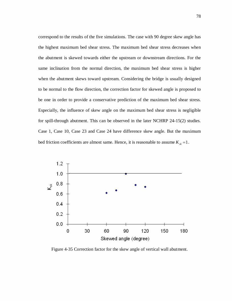
78
correspond to the results of the five simulations. The case with 90 degree skew angle has
the highest maximum bed shear stress. The maximum bed shear stress decreases when
the abutment is skewed towards either the upstream or downstream directions. For the
same inclination from the normal direction, the maximum bed shear stress is higher
when the abutment skews toward upstream. Considering the bridge is usually designed
to be normal to the flow direction, the correction factor for skewed angle is proposed to
be one in order to provide a conservative prediction of the maximum bed shear stress.
Especially, the influence of skew angle on the maximum bed shear stress is negligible
for spill-through abutment. This can be observed in the later NCHRP 24-15(2) studies.
Case 1, Case 10, Case 23 and Case 24 have difference skew angle. But the maximum
bed friction coefficients are almost same. Hence, it is reasonable to assume 1=skK .
Figure 4-35 Correction factor for the skew angle of vertical wall abutment.

79
0.10
0.200.30
0.400.500.6
0
1.02
0.70
0.80
X/Wa
Y/W
a
-2 0 20
1
2
3
4
5 Flow
Abutment
Figure 4-36 Bed friction coefficient (×10-2) contour for 60 degree.
0.100.20
0.300.40
0.500.600.60
0.70
1.10
0.800.
500.40
0.30
0.20
0.10
X/Wa
Y/W
a
-2 0 20
1
2
3
4
5 Flow
Abutment
Figure 4-37 Bed friction coefficient (×10-2) contour for 75 degree.

80
1.28
0.100.20
0.400.40
0.20
0.10
0.60
0.50
0.30
0.50
0.70
X/Wa
Y/W
a
-2 -1 0 1 2 3 40
1
2
3
4
5 Flow
Abutment
Figure 4-38 Bed friction coefficient (×10-2) contour for 105 degree.
1.22
0.100.20
0.400.40
0.20
0.10
0.30
0.50
0.50
X/Wa
Y/W
a
-2 -1 0 1 2 3 40
1
2
3
4
5 Flow
Abutment
Figure 4-39 Bed friction coefficient (×10-2) contour for 120 degree.

81
4.4 Maximum Bed Shear Stress Equation in Rectangular Channel
The basic formula of the equation is giving maxτ for the half square pier in deep
water condition (defined in figure 4-2). After the correction factors for channel
contraction ratio, abutment aspect ratio, skew angle, water depth and abutment shape are
determined, the maximum bed shear stress equation around abutment in rectangular
channel can be generated as follows:
max_2 = ⋅ ⋅ ⋅ ⋅ ⋅f vw Cr sh Fr s skC K K K K K
Vτρ
where maxτ = the maximum bed shear stress at the interface between the water and the
river bottom near the abutment toe.
ρ = mass density of water
V = upstream mean depth velocity
y = upstream water depth
aW = top width of the abutment
aL = projected abutment length normal to the flow direction
rC = contraction ratio; defined as / ( )r total total blockedC Q Q Q= −
Re = Reynolds number, defined as Re /aVW ν=
ν = kinematic viscosity
_f VWC = maximum bed friction coefficient near the toe of vertical wall abutment
under deep water conditions
CrK = correction factor for channel contraction ratio
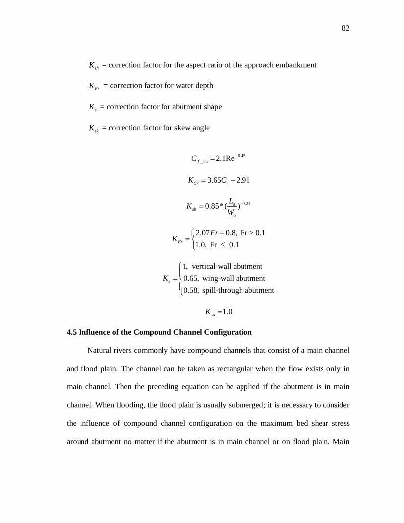
82
shK = correction factor for the aspect ratio of the approach embankment
FrK = correction factor for water depth
sK = correction factor for abutment shape
skK = correction factor for skew angle
45.0
_ Re1.2 −=vwfC
3.65 2.91Cr rK C= −
0.240.85*( )ash
a
LKW
−=
2.07 0.8, Fr > 0.11.0, Fr 0.1
+= ≤
Fr
FrK
1, vertical-wall abutment0.65, wing-wall abutment0.58, spill-through abutment
sK=
0.1=skK
4.5 Influence of the Compound Channel Configuration
Natural rivers commonly have compound channels that consist of a main channel
and flood plain. The channel can be taken as rectangular when the flow exists only in
main channel. Then the preceding equation can be applied if the abutment is in main
channel. When flooding, the flood plain is usually submerged; it is necessary to consider
the influence of compound channel configuration on the maximum bed shear stress
around abutment no matter if the abutment is in main channel or on flood plain. Main
83
channel usually conveys more flow and the unit discharge is generally higher in main
channel than in flood plain. Especially, the flow pattern around the main channel slope
could be quite complex because of the lateral momentum exchange between the main
channel and flood plain. This may have a significant influence on the bed shear stress
around the abutment when the abutment is close to the edge of the main channel.
Contraction ratio is still a good way to describe the blockage effect of the
abutment and the approach embankment in compound channel. As defined in the
methodology section, the contraction ratio is equal to total
total blocked
QQ Q−
at upstream section.
Only discharge is included in the definition, which means it can be applied in any type of
river channel. However, the contraction ratio can only be used to reflect the averaged
blockage effect. The location of the abutment on the compound channel could not be
considered in this way. As mentioned above, the flow field could be very complex when
the abutment toe is very close to the main channel slope. Hence, it may be necessary to
include another correction for the abutment location in compound channel. Obviously,
this is not necessary in the rectangular channel. And this correction is believed to be
negligible when the abutment toe is far away from the main channel slope.
According to the flume tests in NCHRP 24-15(2), the clay surface is very smooth
before scouring. And the difference of water depth is not large for main channel and
flood plain. The velocity measurement shows that transverse depth averaged velocity is
very uniform in the compound channel at upstream section. Hence, the uniform
upstream velocity field is applied at the inlet in the numerical studies of compound
84
channel cases. And, the hydraulic smooth boundary is applied through the entire river
bottom. This makes it reasonable to replace the discharge based contraction ratio by the
area ratio of total
total blocked
AA A−
in the data analysis. And this can make it possible to apply
the maximum bed shear stress equation for rectangular channel in the compound channel
conditions with suitable correction.
The objective of this section is to study the relation between the abutment location
on compound channel and the maximum bed shear stress. One flume test case in
NCHRP 24-15(2) is selected to perform the numerical simulation and the spill-through
abutment in the flume test is replaced by vertical wall abutment to avoid the influence of
abutment shape. The channel is assumed to be symmetric and only half is simulated. The
6ft long vertical wall abutment is sitting in the 12 ft wide flume with main channel water
depth ym of 1.63ft and flood plain water depth yf of 0.96ft. Approach velocity is 1.41ft/s.
Eight cases with different flood plain width Lf are simulated with CHEN3D program.
The width of flood plain Lf varies from 2 ft to 10ft. Table 4-5 lists the parameters and the
simulation results of the eight compound channel cases. The contours of friction
coefficient are given in figure 4-41 to figure 4-48. The location of the maximum bed
shear stress usually appears at the upstream corner of the abutment no matter if the
abutment is in flood plain or in main channel. If the abutment is on flood plain, the main
channel slope in front of the abutment will suffer higher bed shear stress. But the bed
shear stress on main channel slope will be very low if the abutment protrudes into main
channel.

85
Table 4-5 Correction factors of compound channel effect.
As shown in table 4-5, the contraction ratios rC of these eight cases are not same.
The smallest contraction ratio appears when the toe of the abutment lies at the edge of
the main channel slope. As mentioned above, the abutment length, water depth and the
flume width are all kept constant. Then the contraction ratio will always increase no
matter the flood plain width increases or decreases. Hence, rC reaches the lower limit
when =a fL L . And the upper limit of the contraction ratio is achieved when the flood
plain width goes to the limit, either zero or the width of the flume. Meanwhile, the
compound channel becomes rectangular one. But the water depth will be different under
these two limiting conditions. Based on the study of contraction ratio in rectangular
channel, the maximum bed friction coefficient _ maxfC is linear proportional with the
contraction ratio rC . Then the case with the smallest contraction ratio (when f aL L= )
should have the lowest _ maxfC . To investigate the influence of the abutment location, the
influence of the contraction ratio must be excluded by correcting _ maxfC with the
86
correction factor CrK derived from rectangular channel study. When the abutment toe is
far away from the main channel slope, the influence of lateral momentum exchange
between main channel and flood plain should vanish. Actually, this can be observed
clearly after the correction of _ max /f CrC K . It should be noted that the influence of water
depth is not constant for these eight cases. It can fall into two categories, abutment on
flood plain and abutment on main channel. The one with abutment toe right at the edge
of main channel slope should be put in the category of flood plain because the main
channel slope is 1to1 and the water depth at the toe is same to water depth on flood
plain. The results of _ max /f CrC K indicate that the big difference among _ maxfC for these
eight cases results mainly from the difference of contraction ratio. To eliminate the
contribution from water depth and other parameters, it is desirable to normalize the
values of _ max /f CrC K with the one far away from the main channel
slope _ max _ _/f reference Cr referenceC K . The case of 10fL ft= is chosen to normalize the cases
with abutment on flood plain. And the case of 2fL ft= is chosen to normalize the cases
with abutment on main channel. Value of _ max _ max_ _( / ) / ( / )f Cr f reference Cr referenceC K C K is
called abutment location correction factor LK . f a
f
L Ly−
is preferred to represent the
abutment location because it show the relative distance of abutment toe to the main
channel slope. Figure 4-40 shows the relationship between LK and f a
f
L Ly−
. The bed

87
shear stress is about 20% higher when the abutment toe is right at the edge of the main
channel slope. And this influence will exist only in a small range.
Figure 4-40 Correction factor of abutment location in compound channel.
1.99
0.10
0.20
0.40
0.20
0.40 0.60 0.60
0.60
0.801.00
0.60 0.80
1.00
X/Wa
Y/W
a
-4 -3 -2 -1 0 1 2 3 40
1
2
3
4
5
6 Flow
Abutment
Figure 4-41 Bed friction coefficient (×10-2) contour for Lm = 6ft.
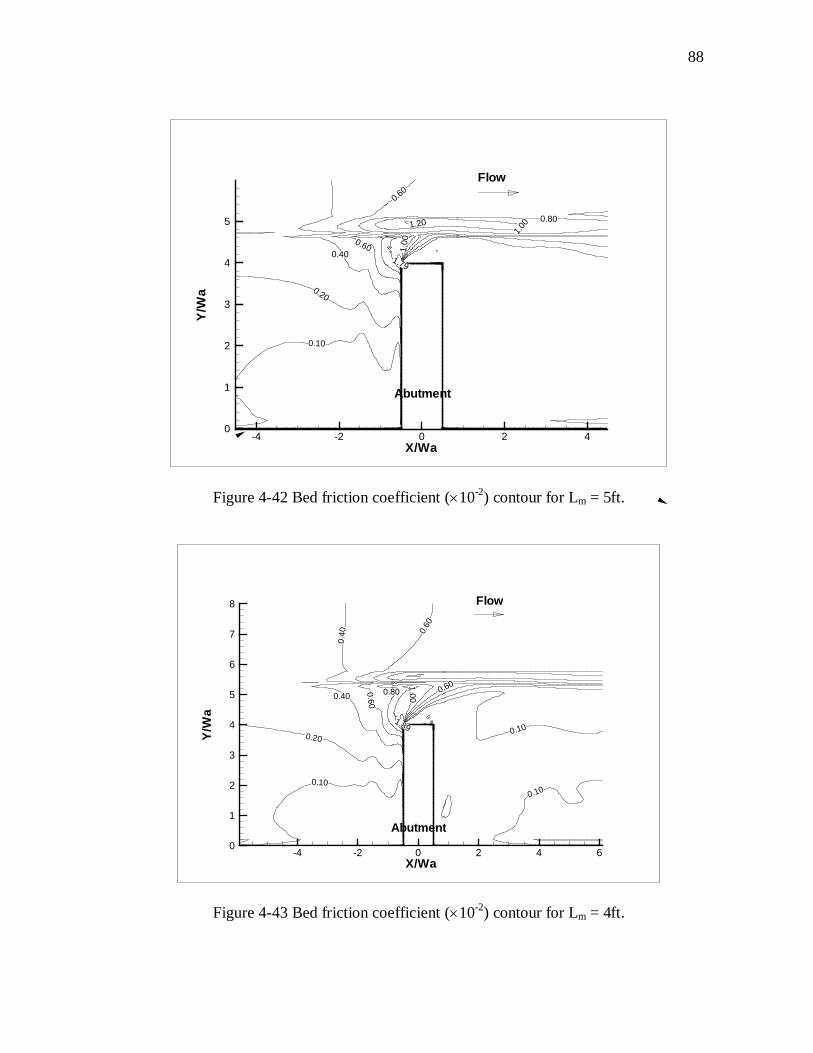
88
1.79
0.10
0.20
0.40
0.60
1.00 0.80
1.20
1.000.60
X/Wa
Y/W
a
-4 -2 0 2 40
1
2
3
4
5
Flow
Abutment
Figure 4-42 Bed friction coefficient (×10-2) contour for Lm = 5ft.
1.89
0.10
0.20
0.40
0.40 0.
60
0.10
0.10
0.60
0.80
1.00 0.60
X/Wa
Y/W
a
-4 -2 0 2 4 60
1
2
3
4
5
6
7
8 Flow
Abutment
Figure 4-43 Bed friction coefficient (×10-2) contour for Lm = 4ft.
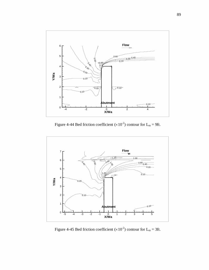
89
2.22
0.10
0.20
0.10
0.20
0.30
0.40
0.60
0.80
0.60 0.400.30
0.10
0.10
0.10
X/Wa
Y/W
a
-4 -2 0 2 40
1
2
3
4
5
6 Flow
Abutment
Figure 4-44 Bed friction coefficient (×10-2) contour for Lm = 9ft.
2.11
0.10
0.20
0.40
0.60
0.10
0.10
0.200.400.60
1.001.20
0.801.00
1.20
X/Wa
Y/W
a
-5 -4 -3 -2 -1 0 1 2 3 4 50
1
2
3
4
5
6
7 Flow
Abutment
Figure 4-45 Bed friction coefficient (×10-2) contour for Lm = 3ft.
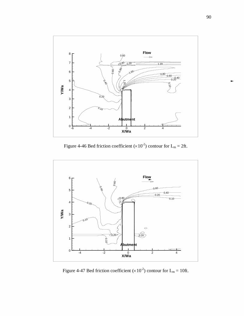
90
2.15
0.10
0.20
0.40
0.60 0.80
1.000.10
0.200.40
0.600.80
1.20
1.201.000.80
0.60
X/Wa
Y/W
a
-6 -4 -2 0 2 40
1
2
3
4
5
6
7
8 Flow
Abutment
Figure 4-46 Bed friction coefficient (×10-2) contour for Lm = 2ft.
2.35
0.10
0.20
0.40
0.60
0.60
0.400.20
0.10
0.20
0.10
0.20
0.80
X/Wa
Y/W
a
-4 -2 0 2 40
1
2
3
4
5
6 Flow
Abutment
Figure 4-47 Bed friction coefficient (×10-2) contour for Lm = 10ft.
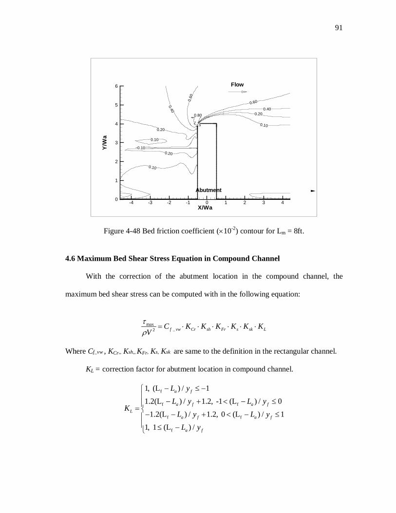
91
1.75
0.10
0.20
0.10
0.20
0.40
0.60
0.60
0.400.20
0.10
0.80
0.10
X/Wa
Y/W
a
-4 -3 -2 -1 0 1 2 3 40
1
2
3
4
5
6 Flow
Abutment
Figure 4-48 Bed friction coefficient (×10-2) contour for Lm = 8ft.
4.6 Maximum Bed Shear Stress Equation in Compound Channel
With the correction of the abutment location in the compound channel, the
maximum bed shear stress can be computed with in the following equation:
max
_2 = ⋅ ⋅ ⋅ ⋅ ⋅ ⋅f vw Cr sh Fr s sk LC K K K K K KV
τρ
Where Cf_vw , KCr,, Ksh,, KFr, Ks, Ksk are same to the definition in the rectangular channel.
KL = correction factor for abutment location in compound channel.
f
f f
f f
f
1, (L ) / 1
1.2(L ) / 1.2, -1 (L ) / 0
1.2(L ) / 1.2, 0 (L ) / 1
1, 1 (L ) /
a f
a f a fL
a f a f
a f
L yL y L y
KL y L y
L y
− ≤ − − + < − ≤= − − + < − ≤ ≤ −

92
It should be noted that the proposed equations in this chapter are based on the
channel contraction ratio defined by the channel cross section area ratio. The reason is
that the water is relatively deep in these simulations and the bed surface roughness is
same for flood plain and main channel. The upstream velocity is found to be uniformly
distributed from the numerical simulations. And this is also true in the flume tests.
Hence the channel conveyance ratio is same to the area ratio. In the engineering practice,
the area ratio may not represent the conveyance ratio very well. So the contraction ratio
should be determined based on the actual conveyance ratio to get better prediction.
4.7 Verification of the Maximum Bed Shear Stress Equation
The proposed equation consists of several correction factors. The assumption is
that these dimensionless parameters are independent and they can be superposed simply.
The verification needs to be conducted to check the performance of this method. And the
data regression of each parameter may not reflect the trend perfectly and have
discrepancy. The simple product of these parameters could accumulate these errors. This
is going to be studied in this section.
One way to check the performance of the equation is to predict the database used
in the equation development. All the cases have been tabulated in table 4-6. Those six
dimensionless parameters have been marked. In the parametric studies, only one
parameter will be changed one time in theory. And the predicted maximum bed friction
coefficients are also listed in the table. The overall performance of the equation is shown
in figure 4-49. The good agreement can be observed for most of the cases. It proves that
the method has been well conducted during the data regressions.
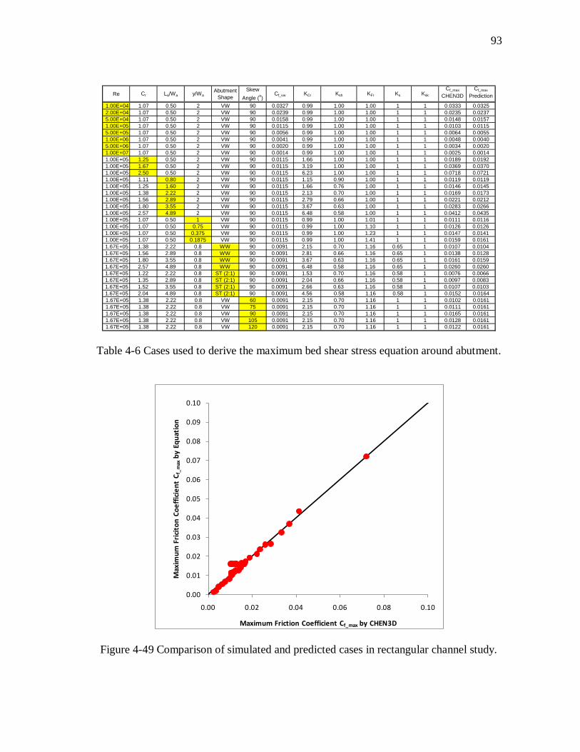
93
Re Cr La/Wa y/WaAbutment
ShapeSkew
Angle (o)Cf_vw KCr Ksh KFr Ks Ksk
Cf_max
CHEN3DCf_max
Prediction
1.00E+04 1.07 0.50 2 VW 90 0.0327 0.99 1.00 1.00 1 1 0.0333 0.03252.00E+04 1.07 0.50 2 VW 90 0.0239 0.99 1.00 1.00 1 1 0.0235 0.02375.00E+04 1.07 0.50 2 VW 90 0.0158 0.99 1.00 1.00 1 1 0.0148 0.01571.00E+05 1.07 0.50 2 VW 90 0.0115 0.99 1.00 1.00 1 1 0.0103 0.01155.00E+05 1.07 0.50 2 VW 90 0.0056 0.99 1.00 1.00 1 1 0.0064 0.00551.00E+06 1.07 0.50 2 VW 90 0.0041 0.99 1.00 1.00 1 1 0.0048 0.00405.00E+06 1.07 0.50 2 VW 90 0.0020 0.99 1.00 1.00 1 1 0.0034 0.00201.00E+07 1.07 0.50 2 VW 90 0.0014 0.99 1.00 1.00 1 1 0.0025 0.00141.00E+05 1.25 0.50 2 VW 90 0.0115 1.66 1.00 1.00 1 1 0.0189 0.01921.00E+05 1.67 0.50 2 VW 90 0.0115 3.19 1.00 1.00 1 1 0.0369 0.03701.00E+05 2.50 0.50 2 VW 90 0.0115 6.23 1.00 1.00 1 1 0.0718 0.07211.00E+05 1.11 0.80 2 VW 90 0.0115 1.15 0.90 1.00 1 1 0.0119 0.01191.00E+05 1.25 1.60 2 VW 90 0.0115 1.66 0.76 1.00 1 1 0.0146 0.01451.00E+05 1.38 2.22 2 VW 90 0.0115 2.13 0.70 1.00 1 1 0.0169 0.01731.00E+05 1.56 2.89 2 VW 90 0.0115 2.79 0.66 1.00 1 1 0.0221 0.02121.00E+05 1.80 3.55 2 VW 90 0.0115 3.67 0.63 1.00 1 1 0.0283 0.02661.00E+05 2.57 4.89 2 VW 90 0.0115 6.48 0.58 1.00 1 1 0.0412 0.04351.00E+05 1.07 0.50 1 VW 90 0.0115 0.99 1.00 1.01 1 1 0.0111 0.01161.00E+05 1.07 0.50 0.75 VW 90 0.0115 0.99 1.00 1.10 1 1 0.0126 0.01261.00E+05 1.07 0.50 0.375 VW 90 0.0115 0.99 1.00 1.23 1 1 0.0147 0.01411.00E+05 1.07 0.50 0.1875 VW 90 0.0115 0.99 1.00 1.41 1 1 0.0159 0.01611.67E+05 1.38 2.22 0.8 WW 90 0.0091 2.15 0.70 1.16 0.65 1 0.0107 0.01041.67E+05 1.56 2.89 0.8 WW 90 0.0091 2.81 0.66 1.16 0.65 1 0.0138 0.01281.67E+05 1.80 3.55 0.8 WW 90 0.0091 3.67 0.63 1.16 0.65 1 0.0161 0.01591.67E+05 2.57 4.89 0.8 WW 90 0.0091 6.48 0.58 1.16 0.65 1 0.0260 0.02601.67E+05 1.22 2.22 0.8 ST (2:1) 90 0.0091 1.53 0.70 1.16 0.58 1 0.0076 0.00661.67E+05 1.35 2.89 0.8 ST (2:1) 90 0.0091 2.04 0.66 1.16 0.58 1 0.0097 0.00831.67E+05 1.52 3.55 0.8 ST (2:1) 90 0.0091 2.66 0.63 1.16 0.58 1 0.0107 0.01031.67E+05 2.04 4.89 0.8 ST (2:1) 90 0.0091 4.56 0.58 1.16 0.58 1 0.0152 0.01641.67E+05 1.38 2.22 0.8 VW 60 0.0091 2.15 0.70 1.16 1 1 0.0102 0.01611.67E+05 1.38 2.22 0.8 VW 75 0.0091 2.15 0.70 1.16 1 1 0.0111 0.01611.67E+05 1.38 2.22 0.8 VW 90 0.0091 2.15 0.70 1.16 1 1 0.0165 0.01611.67E+05 1.38 2.22 0.8 VW 105 0.0091 2.15 0.70 1.16 1 1 0.0128 0.01611.67E+05 1.38 2.22 0.8 VW 120 0.0091 2.15 0.70 1.16 1 1 0.0122 0.0161
Table 4-6 Cases used to derive the maximum bed shear stress equation around abutment.
0.00
0.01
0.02
0.03
0.04
0.05
0.06
0.07
0.08
0.09
0.10
0.00 0.02 0.04 0.06 0.08 0.10
Max
imum
Fri
cito
n Co
effic
ient
Cf_
max
by E
quat
ion
Maximum Friction Coefficient Cf_max by CHEN3D
Figure 4-49 Comparison of simulated and predicted cases in rectangular channel study.
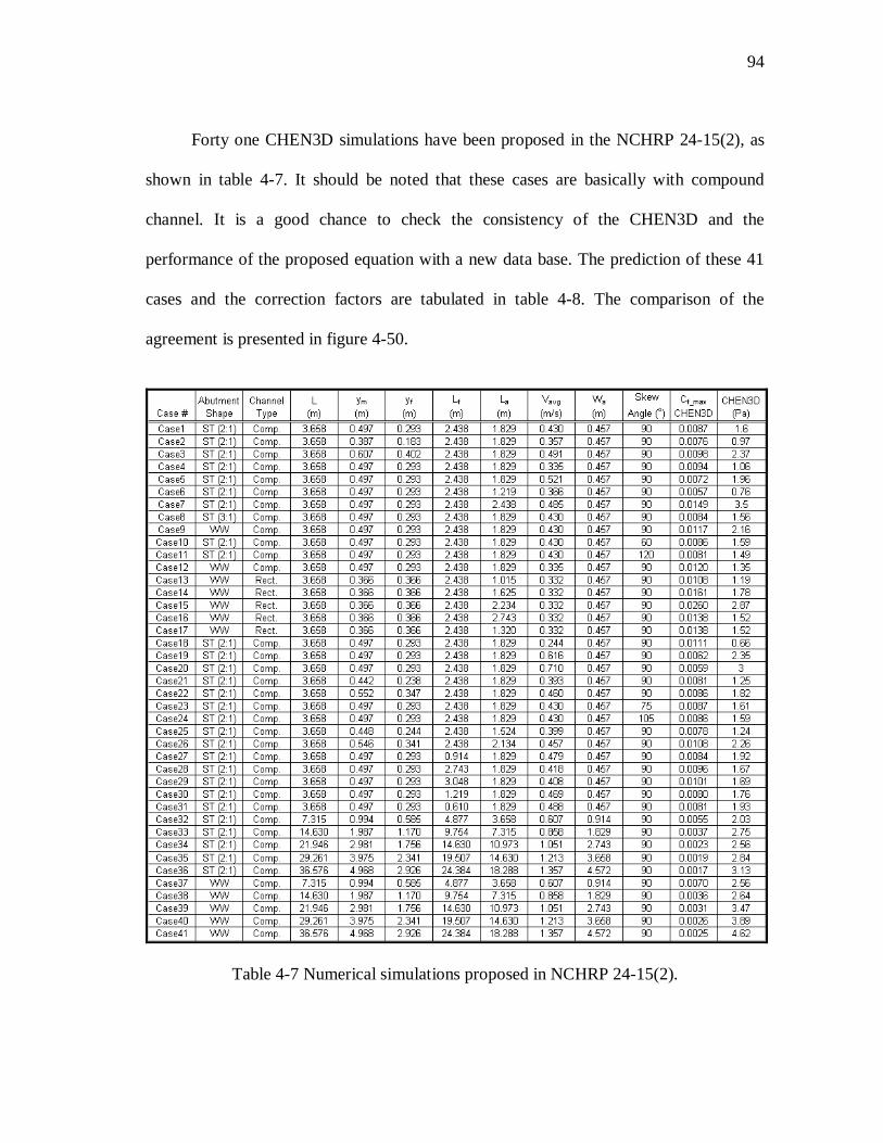
94
Forty one CHEN3D simulations have been proposed in the NCHRP 24-15(2), as
shown in table 4-7. It should be noted that these cases are basically with compound
channel. It is a good chance to check the consistency of the CHEN3D and the
performance of the proposed equation with a new data base. The prediction of these 41
cases and the correction factors are tabulated in table 4-8. The comparison of the
agreement is presented in figure 4-50.
Table 4-7 Numerical simulations proposed in NCHRP 24-15(2).
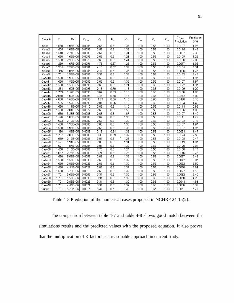
95
Table 4-8 Prediction of the numerical cases proposed in NCHRP 24-15(2).
The comparison between table 4-7 and table 4-8 shows good match between the
simulations results and the predicted values with the proposed equation. It also proves
that the multiplication of K factors is a reasonable approach in current study.

96
0.00
0.01
0.02
0.03
0.04
0.00 0.01 0.02 0.03 0.04
Max
imum
Fri
cito
n Co
effic
ient
Cf_
max
by E
quat
ion
Maximum Friction Coefficient Cf_max by CHEN3D
20%
10%30%
Figure 4-50 Comparison of the simulated and predicted cases in NCHRP 24-15(2).
As shown in figure 4-50, the prediction by equation can match the CHEN3D
simulation reasonably. For some cases, the predicted values can be about 20% to 30%
higher than the simulated values. One possible reason for this discrepancy is that the
influence of the compound channel configuration on the flow redistribution is not
evaluated very well with the channel geometric contraction ratio.
4.8 Real Maximum Bed Shear Stress around Abutment in SRICOS Method
Eighteen flume test cases (Oh, 2008) have been conducted in NCHRP 24-15(2) as
shown in table 4-9. In the original design, these cases are identical to the corresponding
cases in numerical study. During the testing, the flow conditions were changed in several

97
cases for convenience. The detail parameters of these 17 cases are provided in table 4-9
together with the predicted maximum bed shear stresses. The values of maxτ are
calculated according to the actual parameters and the proposed equation. And the
proposed maximum bed shear stresses are independent of the bed materials and based on
hydraulic smooth boundary condition (roughness is not included in the prediction).
Table 4-9 Flume test cases in NCHRP 24-15(2).
Hyperbolic model is found to be able to describe the development of the
maximum scour depth over time in the bridge scour problems (Briaud et al., 1999).
Based on measurements in the flume tests, the initial erosion rate and the maximum
scour depth can be estimated through data regression of the maximum scour depth
history with hyperbola function. Table 4-10 lists all the initial erosion rates iniZ and the
ultimate scour depths maxZ .

98
Case # iniZ (mm/hr)
maxZ(mm)
max _ maxτ(Pa)
max _ minτ(Pa)
maxτ (Pa)EFA
maxτ (Pa) Prediction
max_ max_/EFA predictionτ τ
Case1 5.37 439 22 8 13.59 2.09 6.50 Case1 II 6.16 490 22 8 14.79 2.00 7.40 Case2 0.74 282 9 1.5 6.54 1.46 4.48 Case3 1.05 589 10 2 7.01 2.22 3.16 Case4 1.14 300 10 2 7.15 1.27 5.63 Case5 1.66 808 10 2 7.94 2.72 2.92 Case6 1.25 351 10 2 7.32 1.35 5.42 Case7 4.55 1190 20 5 12.34 3.30 3.74 Case8 2.20 413 11 3 8.76 1.80 4.87 Case9 1.80 667 10 2 8.15 2.61 3.12 Case10 Case11 Case12 0.24 155 4 0.7 5.78 1.64 3.52
Case12B 1.47 1429 10 2 7.65 4.95 1.55 Case13 0.54 66 7 1.1 6.24 1.13 5.52 Case14 2.37 304 11 3 9.02 1.70 5.31 Case15 1.73 334 10 2 8.05 2.51 3.21 Case16 3.21 448 20 3 10.3 2.20 4.68 Case17 1.96 262 11 3 8.40 1.75 4.80
Table 4-10 Maximum bed shear stresses based on EFA results.
Porcelain clay has been chosen in the flume tests. Eleven samples of the clay have
been tested during the entire flume test period from 2005 to 2008 to monitor the change
of erosion property. Some of the samples are quite different from the fresh clay after
long time of storage. The EFA results are shown in figure 4-51 and found to scatter in a
wide range. This shows the difficulty in the erosion problem. Even for a well controlled
lab testing, the erosion property of the same type of soil from the same company could
have such a big difference. The regression curve is given in figure 4-51. Based on the
linear regression, the critical shear stress of the porcelain clay is 5.43 Pa, which is the
shear stress when erosion rate is zero. However, the initiation of the scour is defined as
0.1mm/hr in experimental evaluation of soil erosion property.
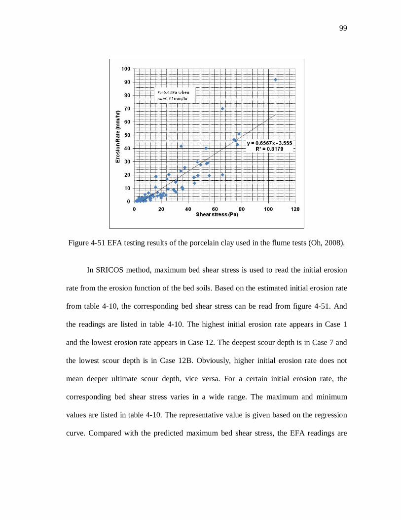
99
Figure 4-51 EFA testing results of the porcelain clay used in the flume tests (Oh, 2008).
In SRICOS method, maximum bed shear stress is used to read the initial erosion
rate from the erosion function of the bed soils. Based on the estimated initial erosion rate
from table 4-10, the corresponding bed shear stress can be read from figure 4-51. And
the readings are listed in table 4-10. The highest initial erosion rate appears in Case 1
and the lowest erosion rate appears in Case 12. The deepest scour depth is in Case 7 and
the lowest scour depth is in Case 12B. Obviously, higher initial erosion rate does not
mean deeper ultimate scour depth, vice versa. For a certain initial erosion rate, the
corresponding bed shear stress varies in a wide range. The maximum and minimum
values are listed in table 4-10. The representative value is given based on the regression
curve. Compared with the predicted maximum bed shear stress, the EFA readings are
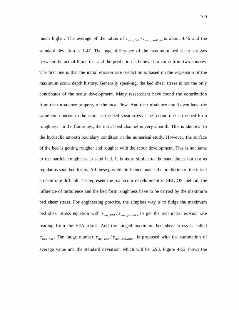
100
much higher. The average of the ratios of max_ max_/EFA predictionτ τ is about 4.46 and the
standard deviation is 1.47. The huge difference of the maximum bed shear stresses
between the actual flume test and the prediction is believed to come from two sources.
The first one is that the initial erosion rate prediction is based on the regression of the
maximum scour depth history. Generally speaking, the bed shear stress is not the only
contributor of the scour development. Many researchers have found the contribution
from the turbulence property of the local flow. And the turbulence could even have the
same contribution to the scour as the bed shear stress. The second one is the bed form
roughness. In the flume test, the initial bed channel is very smooth. This is identical to
the hydraulic smooth boundary condition in the numerical study. However, the surface
of the bed is getting rougher and rougher with the scour development. This is not same
to the particle roughness in sand bed. It is more similar to the sand dunes but not as
regular as sand bed forms. All these possible influence makes the prediction of the initial
erosion rate difficult. To represent the real scour development in SRICOS method, the
influence of turbulence and the bed form roughness have to be carried by the maximum
bed shear stress. For engineering practice, the simplest way is to fudge the maximum
bed shear stress equation with max_ max_/EFA predictionτ τ to get the real initial erosion rate
reading from the EFA result. And the fudged maximum bed shear stress is called
max_ realτ . The fudge number, max_ max_/EFA predictionτ τ , is proposed with the summation of
average value and the standard deviation, which will be 5.93. Figure 4-52 shows the
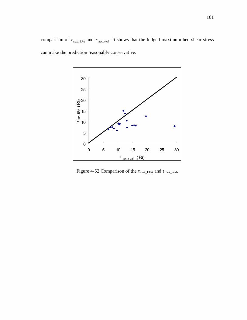
101
comparison of max_ EFAτ and max_ realτ . It shows that the fudged maximum bed shear stress
can make the prediction reasonably conservative.
0
5
10
15
20
25
30
0 5 10 15 20 25 30τmax_r eal ( Pa)
τ max
_EFA
(Pa
)
Figure 4-52 Comparison of the τmax_EFA and τmax_real.
102
CHAPTER V
MAXIMUM BED SHEAR STRESS
AROUND ABUTMENT IN OVERTOPPING FLOW
The bed shear stress around abutment in overtopping flow is studied in this
section. Overtopping is usually defined as the situations when the flow of water is over a
dam or embankment. In current research, overtopping means only the situation when the
bridge deck becomes inundated during the flood; and what concerned is the changing of
bed shear stress around abutment when overtopping occurs. Typical understanding of the
influence of overtopping is that flow is slightly pressurized and higher bed shear stress is
created to aggravate scour conditions. To look into the overtopping problems, different
channel configurations are studied, including overtopping in constant channel,
overtopping in compound channel, overtopping in nonsymetric channel, overtopping in
channel bend. At last the flow at the confluence of the river channel is also studied.
5.1 Verification of the Overtopping Flow Simulation
Kerenyi (personal communication, December, 2007) investigated bed shear stress
distribution under inundated bridge deck with shear stress sensor. The experiment was
conducted in FHWA lab in washington. Bridge model is shown in figure 5-1 and the
notations are explained in figure 5-2. Bed surface was roughened by sands with d50 equal
to 1mm. Approach velocity is 1.44 ft/s; water depth hu is 0.83ft; Froude number is 0.28.
The bridge deck could be adjusted vertically during the testing. The experiments focused
on the influence of the bridge deck elevation on the bed shear stress distribution. Kerenyi
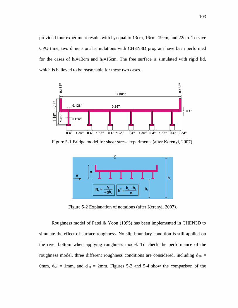
103
provided four experiment results with hb equal to 13cm, 16cm, 19cm, and 22cm. To save
CPU time, two dimensional simulations with CHEN3D program have been performed
for the cases of hb=13cm and hb=16cm. The free surface is simulated with rigid lid,
which is believed to be reasonable for these two cases.
Figure 5-1 Bridge model for shear stress experiments (after Kerenyi, 2007).
Figure 5-2 Explanation of notations (after Kerenyi, 2007).
Roughness model of Patel & Yoon (1995) has been implemented in CHEN3D to
simulate the effect of surface roughness. No slip boundary condition is still applied on
the river bottom when applying roughness model. To check the performance of the
roughness model, three different roughness conditions are considered, including d50 =
0mm, d50 = 1mm, and d50 = 2mm. Figures 5-3 and 5-4 show the comparison of the

104
simulated results with the measurements. All the simulation results can provide the
correct trend. The shear stress will increase significantly under the bridge deck and
decrease at downstream sides. X position of 0cm is the upstream edge of the deck. And
the width of the deck is 26cm. The maxτ occurs under the deck at the upstream half.
Obviously, the smooth boudary condition seriously underestimates the maximum bed
shear stress under the bridge deck. When the ks in the roughness model is taken as d50 =
1mm, the bed shear stress is still underestimated even if there is a big improvement. It
turns out that the prediciton will be in good agreement with measurement when taking
d50 = 2mm. These two simulations of overtopping cases show the significant influence of
bed roughness on the bed shear stress. And this influence is closely related to the deck
location. Also, the current roughness model needs further refinement because the
roughness has to be exaggerated to yield the real roughness effects.
Figure 5-3 Bed shear stress distribution of hb = 13cm.
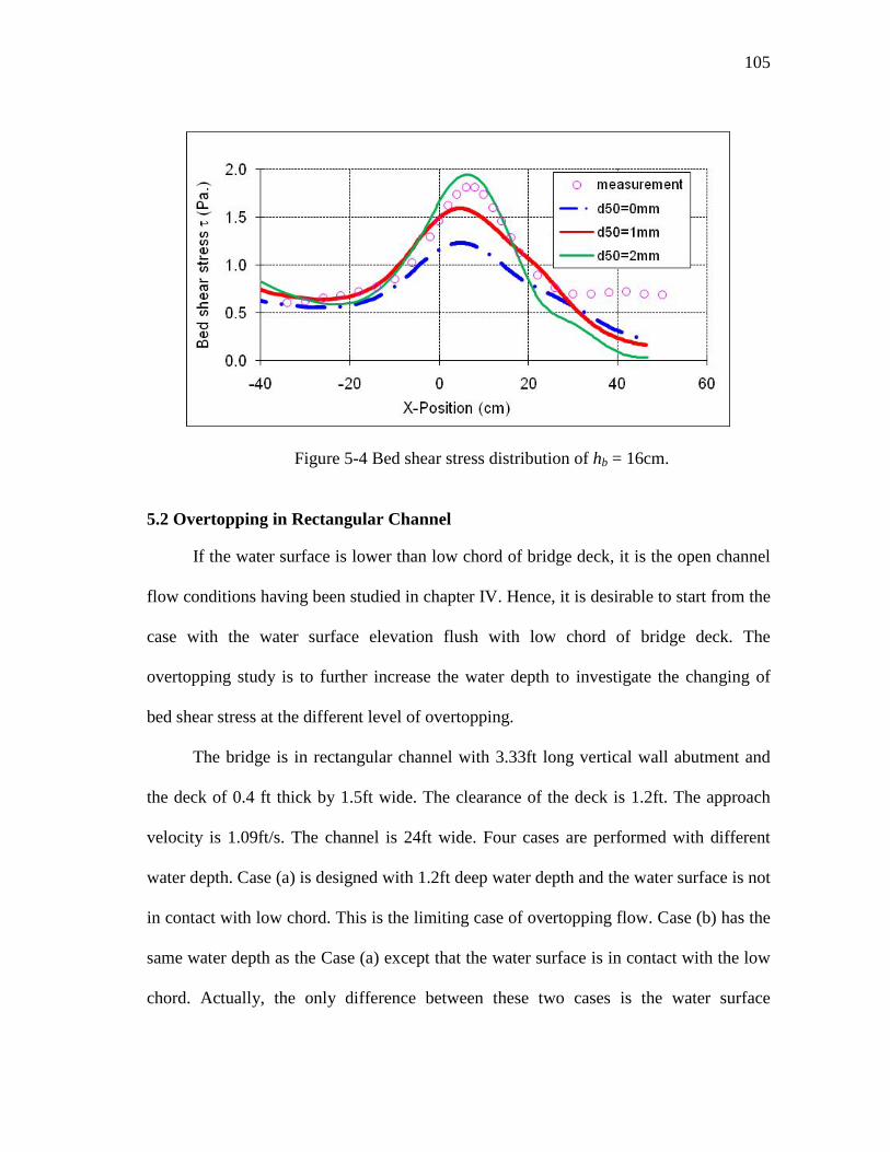
105
Figure 5-4 Bed shear stress distribution of hb = 16cm.
5.2 Overtopping in Rectangular Channel
If the water surface is lower than low chord of bridge deck, it is the open channel
flow conditions having been studied in chapter IV. Hence, it is desirable to start from the
case with the water surface elevation flush with low chord of bridge deck. The
overtopping study is to further increase the water depth to investigate the changing of
bed shear stress at the different level of overtopping.
The bridge is in rectangular channel with 3.33ft long vertical wall abutment and
the deck of 0.4 ft thick by 1.5ft wide. The clearance of the deck is 1.2ft. The approach
velocity is 1.09ft/s. The channel is 24ft wide. Four cases are performed with different
water depth. Case (a) is designed with 1.2ft deep water depth and the water surface is not
in contact with low chord. This is the limiting case of overtopping flow. Case (b) has the
same water depth as the Case (a) except that the water surface is in contact with the low
chord. Actually, the only difference between these two cases is the water surface

106
boundary condition under the deck. Case (c) has water depth of 1.6 ft and water surface
flush with deck surface. In this case, the flow is not overtopping the deck. Case (d) has
water depth of 2.0ft. The water surface is 0.4 ft higher than the deck surface. All the
parameters in these four cases have been given in figure 5-5. The diagrams are the
transvert cross sections at the middle of abutment. The channel is in symmetry and only
half is shown.
Figure 5-5 Cross sections at the middle of the abutment for rectangular channels.
0.4ft
0.4ft
0.4ft
0.4ft
(a)
(b)
(c)
(d)
1.2ft
1.2ft
1.2ft
1.2ft
V=1.09ft/s, Wa=1.5ft, VW Abutment La=3.33ft
La=3.33ft
La=3.33ft
La=3.33ft
V=1.09ft/s, Wa=1.5ft, VW Abutment
V=1.09ft/s, Wa=1.5ft, VW Abutment
V=1.09ft/s, Wa=1.5ft, VW Abutment
L=12ft
L=12ft
L=12ft
L=12ft
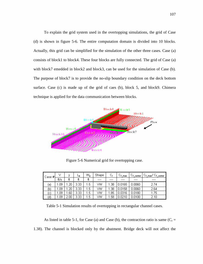
107
To explain the grid system used in the overtopping simulations, the grid of Case
(d) is shown in figure 5-6. The entire computation domain is divided into 10 blocks.
Actually, this grid can be simplified for the simulation of the other three cases. Case (a)
consists of block1 to block4. These four blocks are fully connected. The grid of Case (a)
with block7 emedded in block2 and block3, can be used for the simulation of Case (b).
The purpose of block7 is to provide the no-slip boundary condition on the deck bottom
surface. Case (c) is made up of the grid of caes (b), block 5, and block9. Chimera
technique is applied for the data communication between blocks.
Figure 5-6 Numerical grid for overtopping case.
Table 5-1 Simulation results of overtopping in rectangular channel cases.
As listed in table 5-1, for Case (a) and Case (b), the contraction ratio is same (Cr =
1.38). The channel is blocked only by the abutment. Bridge deck will not affect the
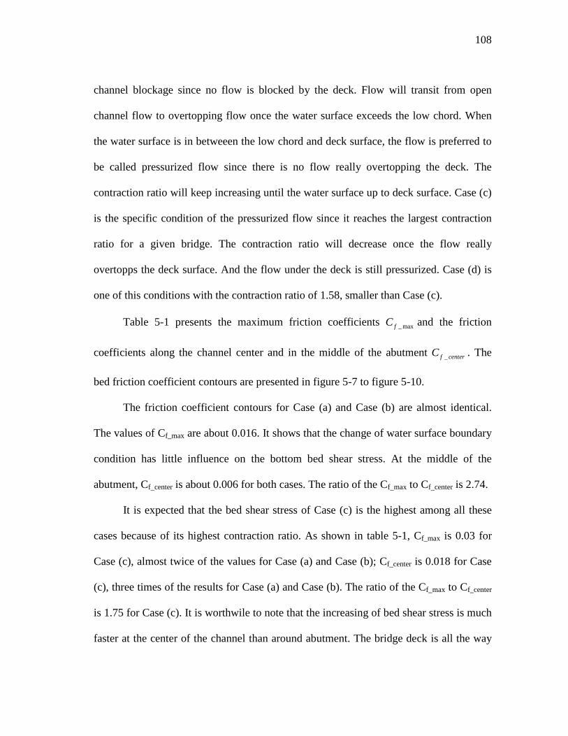
108
channel blockage since no flow is blocked by the deck. Flow will transit from open
channel flow to overtopping flow once the water surface exceeds the low chord. When
the water surface is in betweeen the low chord and deck surface, the flow is preferred to
be called pressurized flow since there is no flow really overtopping the deck. The
contraction ratio will keep increasing until the water surface up to deck surface. Case (c)
is the specific condition of the pressurized flow since it reaches the largest contraction
ratio for a given bridge. The contraction ratio will decrease once the flow really
overtopps the deck surface. And the flow under the deck is still pressurized. Case (d) is
one of this conditions with the contraction ratio of 1.58, smaller than Case (c).
Table 5-1 presents the maximum friction coefficients _ maxfC and the friction
coefficients along the channel center and in the middle of the abutment _f centerC . The
bed friction coefficient contours are presented in figure 5-7 to figure 5-10.
The friction coefficient contours for Case (a) and Case (b) are almost identical.
The values of Cf_max are about 0.016. It shows that the change of water surface boundary
condition has little influence on the bottom bed shear stress. At the middle of the
abutment, Cf_center is about 0.006 for both cases. The ratio of the Cf_max to Cf_center is 2.74.
It is expected that the bed shear stress of Case (c) is the highest among all these
cases because of its highest contraction ratio. As shown in table 5-1, Cf_max is 0.03 for
Case (c), almost twice of the values for Case (a) and Case (b); Cf_center is 0.018 for Case
(c), three times of the results for Case (a) and Case (b). The ratio of the Cf_max to Cf_center
is 1.75 for Case (c). It is worthwile to note that the increasing of bed shear stress is much
faster at the center of the channel than around abutment. The bridge deck is all the way
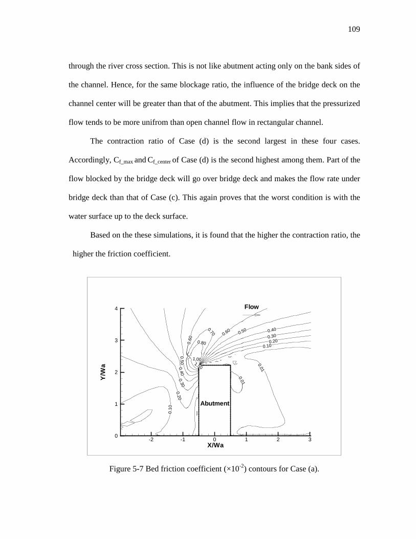
109
through the river cross section. This is not like abutment acting only on the bank sides of
the channel. Hence, for the same blockage ratio, the influence of the bridge deck on the
channel center will be greater than that of the abutment. This implies that the pressurized
flow tends to be more unifrom than open channel flow in rectangular channel.
The contraction ratio of Case (d) is the second largest in these four cases.
Accordingly, Cf_max and Cf_center of Case (d) is the second highest among them. Part of the
flow blocked by the bridge deck will go over bridge deck and makes the flow rate under
bridge deck than that of Case (c). This again proves that the worst condition is with the
water surface up to the deck surface.
Based on the these simulations, it is found that the higher the contraction ratio, the
higher the friction coefficient.
1.50
0.01
0.100.20
0.300.40
0.500.600.70
0.80
1.00
0.10
0.200.30
0.400.50
0.60
0.01
X/Wa
Y/W
a
-2 -1 0 1 2 30
1
2
3
4 Flow
Abutment
Figure 5-7 Bed friction coefficient (×10-2) contours for Case (a).
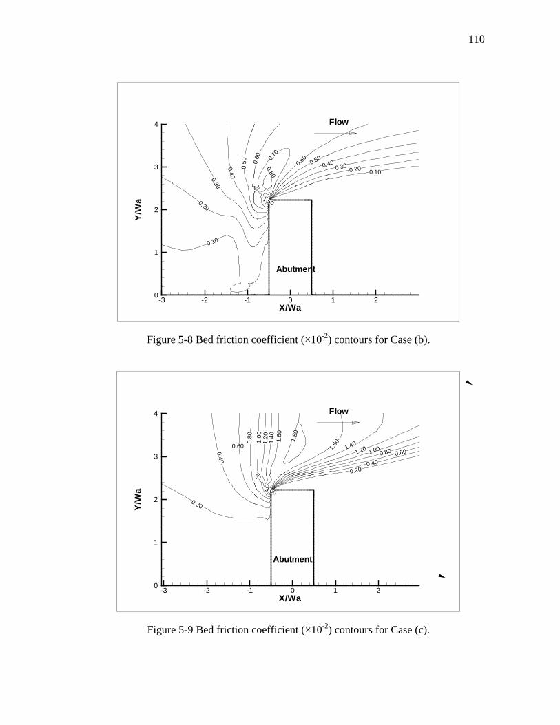
110
0.10
0.20
0.30
0.40
0.50 0.
60 0.70
0.60
0.500.40
0.300.20 0.10
0.80
1.50
X/Wa
Y/W
a
-3 -2 -1 0 1 20
1
2
3
4 Flow
Abutment
Figure 5-8 Bed friction coefficient (×10-2) contours for Case (b).
0.20
0.40
0.60
0.80
1.00
1.20
1.40 1.60
1.80
1.60
1.401.20 1.00
0.80 0.60
0.400.20
3.00
X/Wa
Y/W
a
-3 -2 -1 0 1 20
1
2
3
4 Flow
Abutment
Figure 5-9 Bed friction coefficient (×10-2) contours for Case (c).

111
2.100.
10
0.20
0.40 0.60
0.80 1.00
1.00
0.800.60
0.40 0.20 0.10
0.10
X/Wa
Y/W
a
-3 -2 -1 0 1 2
1
2
3
4 Flow
Abutment
Figure 5-10 Bed friction coefficient (×10-2) contours for Case (d).
Table 5-2 Prediction of Cf_max in rectangluar channel cases with overtoppping.
To predict the maximum bed shear stress around abutment under overtopping
conditions, the equation proposed in Chapter IV is applied. The basic ideal is to assume
that the overtopping condition is equivalent to open channel flow condition with same
contraction ratio. The detailed calculation is presented in table 5-2. The predicted
maximum friction coefficients are close to the simulated results. The comparison is
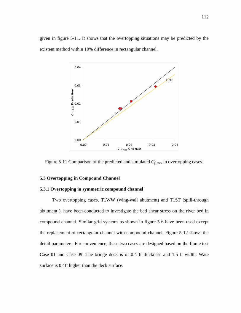
112
given in figure 5-11. It shows that the overtopping situations may be predicted by the
existent method within 10% difference in rectangular channel.
0.00
0.01
0.02
0.03
0.04
0.00 0.01 0.02 0.03 0.04C f_max C HE N3D
C f_
max
Pre
dic
tio
n
10%
Figure 5-11 Comparison of the predicted and simulated Cf_max in overtopping cases.
5.3 Overtopping in Compound Channel
5.3.1 Overtopping in symmetric compound channel
Two overtopping cases, T1WW (wing-wall abutment) and T1ST (spill-through
abutment ), have been conducted to investigate the bed shear stress on the river bed in
compound channel. Similar grid systems as shown in figure 5-6 have been used except
the replacement of rectangular channel with compound channel. Figure 5-12 shows the
detail parameters. For convenience, these two cases are designed based on the flume test
Case 01 and Case 09. The bridge deck is of 0.4 ft thickness and 1.5 ft width. Wate
surface is 0.4ft higher than the deck surface.

113
Figure 5-12 Cross sections at the middle of the abutment for compound channels.
Figures 5-13 to 5-16 present the bed shear stress contours for T1WW, Case 09,
T1ST, and Case 01. The bed shear stresses around abutment increase significantly from
open channel flow to the designed overtopping flow. For wing-wall abutment, Cf_max
increases from Case 09 of 0.0117 to T1WW of 0.018; for spill-through abutment, Cf_max
increases from Case 01 of 0.0097 to T1ST of 0.016. At channel center, however, the
change of the bed shear stress on the main channel is not as remarkable as on the
rectangular channel. Cf_center increases from about 0.004 to 0.005 for Case 09 and Case
01 to around 0.006 for T1WW and T1ST.
Regarding the bed shear stresses on the main channel slope, higher values can still
be found in overtopping flow same as the observation on open channel flow. This
indicates that the erosion of main channel slope will still be faster under overtopping
flow conditions.
V=1.41ft/s, Wa=1.5ft, WW Abutment
V=1.41ft/s, Wa=1.5ft, ST(2H:1V) Abutment
La=6ft
L=12ft
L=12ft
La=6ft
0.96ft
0.96ft
1.63ft
0.4ft
0.4ft
1.63ft
0.4ft 0.4ft
T1WW
T1ST
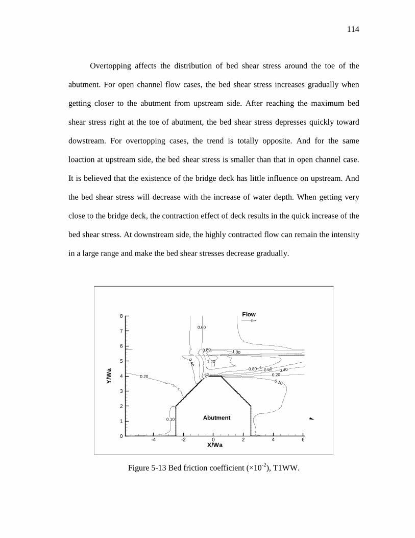
114
Overtopping affects the distribution of bed shear stress around the toe of the
abutment. For open channel flow cases, the bed shear stress increases gradually when
getting closer to the abutment from upstream side. After reaching the maximum bed
shear stress right at the toe of abutment, the bed shear stress depresses quickly toward
dowstream. For overtopping cases, the trend is totally opposite. And for the same
loaction at upstream side, the bed shear stress is smaller than that in open channel case.
It is believed that the existence of the bridge deck has little influence on upstream. And
the bed shear stress will decrease with the increase of water depth. When getting very
close to the bridge deck, the contraction effect of deck results in the quick increase of the
bed shear stress. At downstream side, the highly contracted flow can remain the intensity
in a large range and make the bed shear stresses decrease gradually.
0.10
0.20
0.40
0.60
0.80 1.00
1.20
1.800.80 0.60 0.40
0.200.10
X/Wa
Y/W
a
-4 -2 0 2 4 60
1
2
3
4
5
6
7
8 Flow
Abutment
Figure 5-13 Bed friction coefficient (×10-2), T1WW.
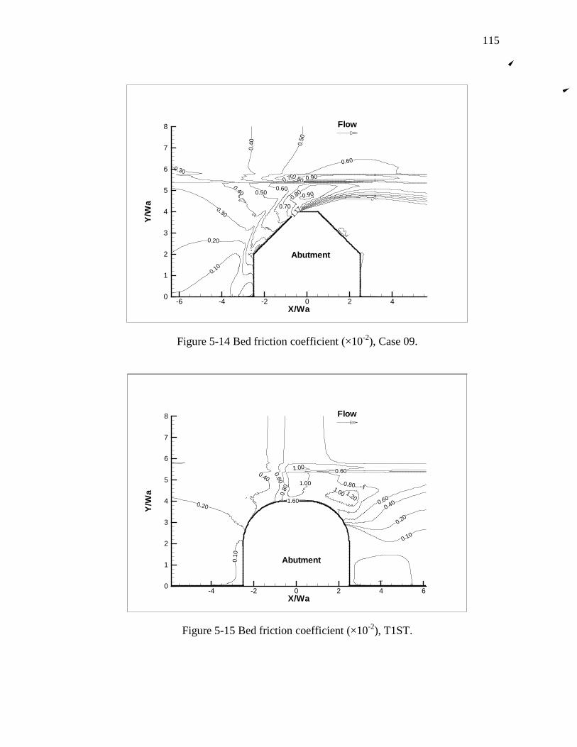
115
0.10
0.20
0.30
0.40 0.500.60
0.700.80 0.90
0.30
0.40 0.
50
0.60
0.700.80 0.90
1.17
X/Wa
Y/W
a
-6 -4 -2 0 2 40
1
2
3
4
5
6
7
8 Flow
Abutment
Figure 5-14 Bed friction coefficient (×10-2), Case 09.
0.10
0.20
0.40
0.60
0.80
1.001.00
1.00
1.601.20
0.80
0.60
0.600.40
0.20
0.10
X/Wa
Y/W
a
-4 -2 0 2 4 60
1
2
3
4
5
6
7
8 Flow
Abutment
Figure 5-15 Bed friction coefficient (×10-2), T1ST.
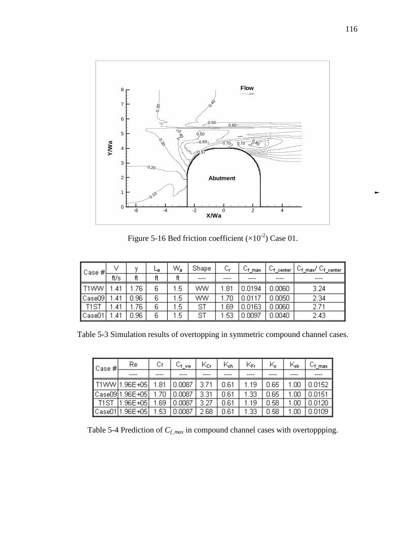
116
0.10
0.20
0.30
0.40 0.50
0.60
0.30 0.4
0
0.50 0.60
0.700.800.70
0.97
X/Wa
Y/W
a
-6 -4 -2 0 2 40
1
2
3
4
5
6
7
8 Flow
Abutment
Figure 5-16 Bed friction coefficient (×10-2) Case 01.
Table 5-3 Simulation results of overtopping in symmetric compound channel cases.
Table 5-4 Prediction of Cf_max in compound channel cases with overtoppping.
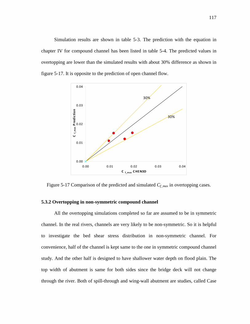
117
Simulation results are shown in table 5-3. The prediction with the equation in
chapter IV for compound channel has been listed in table 5-4. The predicted values in
overtopping are lower than the simulated results with about 30% difference as shown in
figure 5-17. It is opposite to the prediction of open channel flow.
0.00
0.01
0.02
0.03
0.04
0.00 0.01 0.02 0.03 0.04
C f_max C HE N3D
C f_
max
Pre
dic
tio
n
30%
30%
Figure 5-17 Comparison of the predicted and simulated Cf_max in overtopping cases.
5.3.2 Overtopping in non-symmetric compound channel
All the overtopping simulations completed so far are assumed to be in symmetric
channel. In the real rivers, channels are very likely to be non-symmetric. So it is helpful
to investigate the bed shear stress distribution in non-symmetric channel. For
convenience, half of the channel is kept same to the one in symmetric compound channel
study. And the other half is designed to have shallower water depth on flood plain. The
top width of abutment is same for both sides since the bridge deck will not change
through the river. Both of spill-through and wing-wall abutment are studies, called Case

118
T2ST and Case T2WW respectively. The parameters are given on figure 5-18, showing
the cross sections in the middle of the abutment. And figure 5-18 is looking
upstreamward. The grid system is similar to the one for rectangular channel shown in
figure 5-6 except that the full channel is simulated. Rigid lid is still applied on the water
surface. No slip boundary condition is applied on the solid surface.
C L
V=1.41ft/s, Wa=1.5ft, WW Abutment
La=6ft La=6ft 1.63ft
0.96ft 0.64ft
0.4ft 0.4ft
Lf=7.68ft Lf=8ft 3.33ft 3.33ft 0.99ft 0.67ft
Lf=7.68ft Lf=8ft 3.33ft 3.33ft 0.99ft 0.67ft
0.4ft 0.4ft V=1.41ft/s, Wa=1.5ft, ST (2H:1V) Abutment
0.96ft 1.63ft
0.64ft La=5.36ft La=6ft
FL
Figure 5-18 Cross sections for non-symmetric compound channels.
0.20
0.20
0.20
0.40
0.20
0.10
0.400.60 0.40
0.600.801.
001.20
0.100.20
0.400.60
0.600.80
1.30
0.80
X/Wa
Y/W
a
-10 -5 0 5 100
2
4
6
8
10
12
14
16
Flow
Abutment
Abutment
Figure 5-19 Bed friction coefficient (×10-2) contours, T2WW.
Left
Right
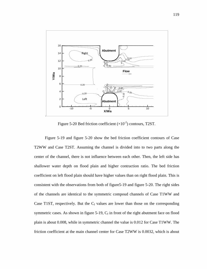
119
.
0.20
0.20
0.20
0.20
0.400.
601.1
0
1.00 0.80 0.60
0.40 0.20
0.10
0.40
0.60
0.80
0.400.200.10
X/Wa
Y/W
a
-10 -5 0 5 100
2
4
6
8
10
12
14
16
Flow
Abutment
Abutment
Figure 5-20 Bed friction coefficient (×10-2) contours, T2ST.
Figure 5-19 and figure 5-20 show the bed friction coefficient contours of Case
T2WW and Case T2ST. Assuming the channel is divided into to two parts along the
center of the channel, there is not influence between each other. Then, the left side has
shallower water depth on flood plain and higher contraction ratio. The bed friction
coefficient on left flood plain should have higher values than on right flood plain. This is
consistent with the observations from both of figure5-19 and figure 5-20. The right sides
of the channels are identical to the symmetric compoud channels of Case T1WW and
Case T1ST, respectively. But the Cf values are lower than those on the corresponding
symmetric cases. As shown in figure 5-19, Cf in front of the right abutment face on flood
plain is about 0.008, while in symmetric channel the value is 0.012 for Case T1WW. The
friction coefficient at the main channel center for Case T2WW is 0.0032, which is about
Left
Right
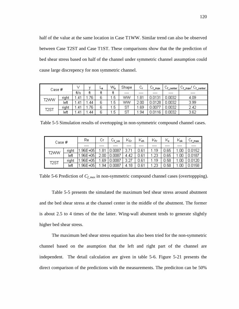
120
half of the value at the same location in Case T1WW. Similar trend can also be observed
between Case T2ST and Case T1ST. These comparisons show that the the prediction of
bed shear stress based on half of the channel under symmetric channel assumption could
cause large discrepency for non symmetric channel.
Table 5-5 Simulation results of overtopping in non-symmetric compound channel cases.
Table 5-6 Prediction of Cf_max in non-symmetric compound channel cases (overtoppping).
Table 5-5 presents the simulated the maximum bed shear stress around abutment
and the bed shear stress at the channel center in the middle of the abutment. The former
is about 2.5 to 4 times of the the latter. Wing-wall abument tends to generate slightly
higher bed shear stress.
The maximum bed shear stress equation has also been tried for the non-symmetric
channel based on the asumption that the left and right part of the channel are
independent. The detail calculation are given in table 5-6. Figure 5-21 presents the
direct comparison of the predictions with the measurements. The prediciton can be 50%

121
higher than the simulated results. This is contrary to the findings in the previous study of
ovetopping in rectangular channel and in symmetric compound channel.
0.00
0.01
0.02
0.03
0.04
0.00 0.01 0.02 0.03 0.04
C f_max C HE N3D
C f_
max
Pre
dic
tio
n
50%
Figure 5-21 Comparison of the predicted and simulated Cf_max in overtopping cases.
5.4 Open Channel Flow on Channel Bend
Channel bend can redistribute the flow along the cross section and further change
the bed shear stress distribution. In the abutment scour analysis, it is interesting to look
into the influence of channel bend on the bed shear stress around abutment. The
geometry of the channel bend is usually characterized by the ratio of R/W. R is the
radius of the bend and W is the width of the channel. Two types of bend are studies in
current research with the R/W equal to 1:1 and 2:1. The bend is fixed with the angle of
90 degree from the inlet to the outlet. The location of the abutment on the channel bend
will also be studied. Two representive locations, middle of the bend and downstream end
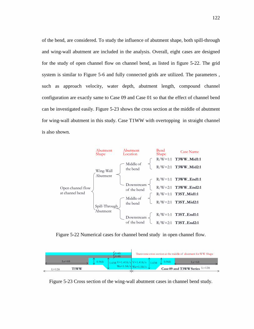
122
of the bend, are considered. To study the influence of abutment shape, both spill-through
and wing-wall abutment are included in the analysis. Overall, eight cases are designed
for the study of open channel flow on channel bend, as listed in figure 5-22. The grid
system is similar to Figure 5-6 and fully connected grids are utilized. The parameters ,
such as approach velocity, water depth, abutment length, compound channel
configuration are exactly same to Case 09 and Case 01 so that the effect of channel bend
can be investigated easily. Figure 5-23 shows the cross section at the middle of abutment
for wing-wall abutment in this study. Case T1WW with overtopping in straight channel
is also shown.
Open channel flow at channel bend
AbutmentShape
Spill-Through Abutment
Middle of the bend
Downstream of the bend
Middle of the bend
Downstream of the bend
R/W=1:1 T3WW_Mid1:1
R/W=2:1 T3WW_Mid2:1
R/W=1:1 T3ST_Mid1:1
R/W=2:1 T3ST_Mid2:1
R/W=1:1 T3WW_End1:1
R/W=2:1 T3WW_End2:1
R/W=1:1 T3ST_End1:1
R/W=2:1 T3ST_End2:1
AbutmentLocation
BendShape
Wing-Wall Abutment
Case Name
Figure 5-22 Numerical cases for channel bend study in open channel flow.
0.96ftV=1.41ft/sV=1.41ft/sWa=1.5ft/s Wa=1.5ft/s
0.4ft0.4ft
L=12ft L=12ft
La=6ft
Case 09 and T3WW Series
0.96ftLa=6ft 1.63ft1.63ft
Transverse cross section at the middle of abutment for WW Shape
T1WW
Figure 5-23 Cross section of the wing-wall abutment cases in channel bend study.
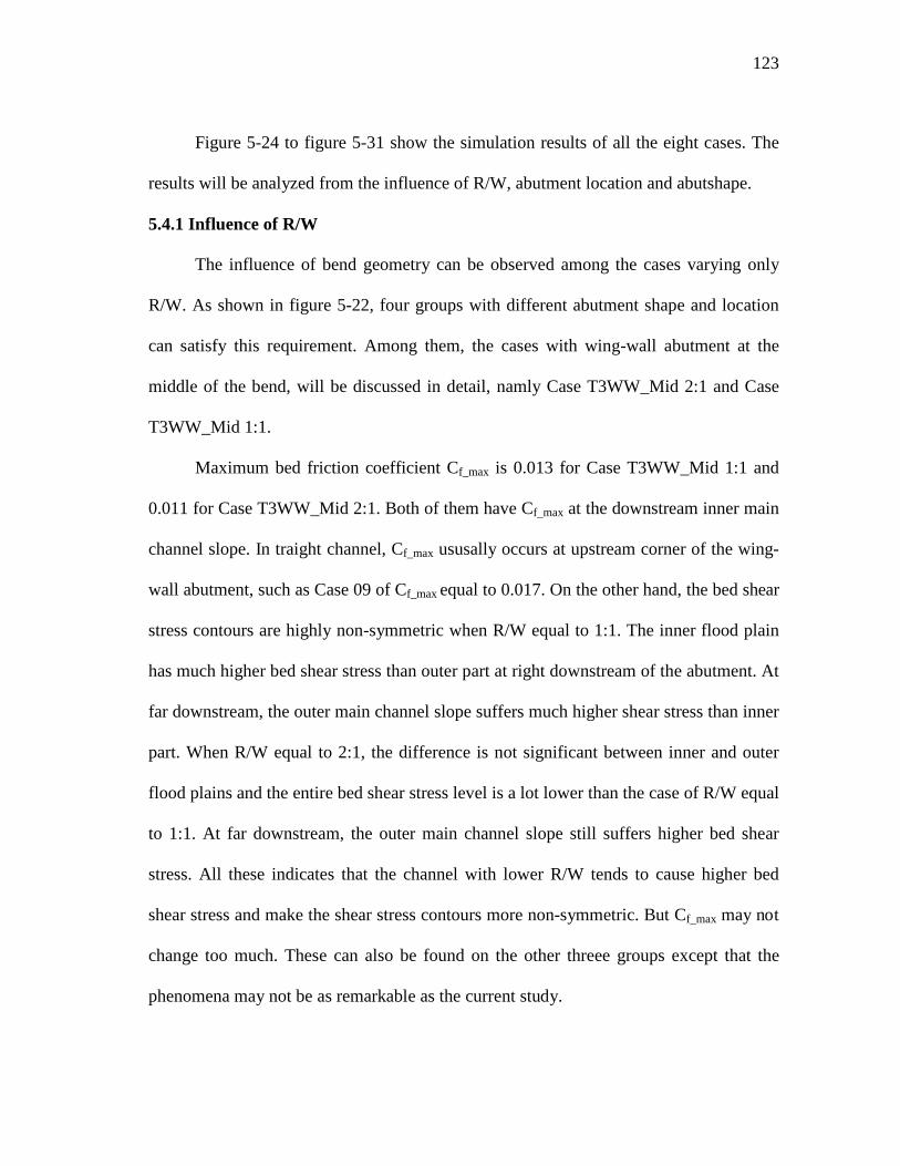
123
Figure 5-24 to figure 5-31 show the simulation results of all the eight cases. The
results will be analyzed from the influence of R/W, abutment location and abutshape.
5.4.1 Influence of R/W
The influence of bend geometry can be observed among the cases varying only
R/W. As shown in figure 5-22, four groups with different abutment shape and location
can satisfy this requirement. Among them, the cases with wing-wall abutment at the
middle of the bend, will be discussed in detail, namly Case T3WW_Mid 2:1 and Case
T3WW_Mid 1:1.
Maximum bed friction coefficient Cf_max is 0.013 for Case T3WW_Mid 1:1 and
0.011 for Case T3WW_Mid 2:1. Both of them have Cf_max at the downstream inner main
channel slope. In traight channel, Cf_max ususally occurs at upstream corner of the wing-
wall abutment, such as Case 09 of Cf_max equal to 0.017. On the other hand, the bed shear
stress contours are highly non-symmetric when R/W equal to 1:1. The inner flood plain
has much higher bed shear stress than outer part at right downstream of the abutment. At
far downstream, the outer main channel slope suffers much higher shear stress than inner
part. When R/W equal to 2:1, the difference is not significant between inner and outer
flood plains and the entire bed shear stress level is a lot lower than the case of R/W equal
to 1:1. At far downstream, the outer main channel slope still suffers higher bed shear
stress. All these indicates that the channel with lower R/W tends to cause higher bed
shear stress and make the shear stress contours more non-symmetric. But Cf_max may not
change too much. These can also be found on the other threee groups except that the
phenomena may not be as remarkable as the current study.
124
The influence of the bend geometry can also be observed from the flow field
either on the plan view of water suface or on the cross section plots. For the straight
channel, the ratio of R/W is equal to infinity. The flow distribution in the transverse
direction will be symmetric as long as the channel and abutment is in symmetry.
However, the symmetric flow will be disturbed when passing the channel bend. At the
beginning of the bend, the inner part of the channel will have higher velocity. Then the
higher velocity region will move to the outer side along with the bend. This can be
observed from approach section of Case T3WW_Mid 1:1. The unit flow rate at the inner
half of the channel is higher than the outer half. However, for Case T3WW_Mid 2:1, the
flow distribution is still in symmetry even if approaching the abutment. This indicates
the sharp bend can cause higher asymmetric flow, which is consistant with the finding in
bed shear stress distribution.
Velocity plan view of Case T3WW_Mid 1:1 shows highly non-symmetric pattern
at the downstream. The highest velocity appears at the inner side of the main channel
and close to the main channel slope. The higher velocity region is very strong and
extending from main channel to the outside flood plain. This indicates that the change of
flow could not follow change of the channel geometry if the R/W is small.
For Case T3WW_Mid 2:1, the flow at the downstream is close to symmetric.The
highest velocity appears in the middle of the main channel with the contours skewed
slightly to the inner abutment. And the higher velocity region bascically remains in the
main channel at the downstream side. All these show that the influence of bend with
R/W equal to 2:1 is not as significant as the bend of R/W equal to 1:1.
125
5.4.2 Influence of abutment location
When the bridge is located at the middle of the bend, the bend turns 45 degree
from the inlet to the location of abutment. The main flow direction may not change as
large as 45 degree because of the delay of the bend effect. The bed shear stress
distribution around the inner and outer abutment will be different since the flow field is
not going to be as symmetric as in straight channel. The magnitude of the bed shear
stress could be affected by lots of other factors, such as R/W ratio , and abutment shape.
But the bed shear stresses around the inner abutment always tend to be higher than the
values around the outer abutment. This can be observed from all the four simulations
with the abutment in the middle of the channel bend. In straight channel, the maximum
bed shear stress usually appears at the upstream corner of the abutment, especially for
the abutments with sharp corner, such as vertical wall and wing-wall abutments. For the
abutment in the middle of the channel bend, however, the maximum bed shear stress
appears at downstream inner main channel slope. This is closly related to the flow field
of bend channel. When approaching the middle of the channel bend, the inner side of the
main channel already has higher velocity than outer side. The high velocity region will
continue to move gradually from inner to outer part along the bend. The existing of the
inner abutment further forces the flow going toward outer bank. However, the local
accelaration at the upstream corner of the inner abutment is not as intensive as in the
straight channel. Obviously, the deflected higher velcoity region does not reach the outer
over bank when passing the middle of the bend since the local flow is not highly
accelerated yet. So, the outer abutment will have little influence on the deflected flow.
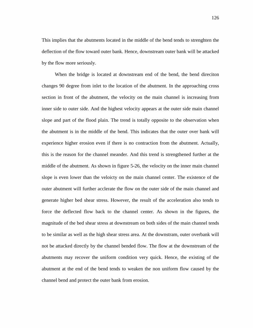
126
This implies that the abutments located in the middle of the bend tends to strenghten the
deflection of the flow toward outer bank. Hence, downstream outer bank will be attacked
by the flow more seriously.
When the bridge is located at downstream end of the bend, the bend direciton
changes 90 degree from inlet to the location of the abutment. In the approaching cross
section in front of the abutment, the velocity on the main channel is increasing from
inner side to outer side. And the highest velocity appears at the outer side main channel
slope and part of the flood plain. The trend is totally opposite to the observation when
the abutment is in the middle of the bend. This indicates that the outer over bank will
experience higher erosion even if there is no contraction from the abutment. Actually,
this is the reason for the channel meander. And this trend is strengthened further at the
middle of the abutment. As shown in figure 5-26, the velocity on the inner main channel
slope is even lower than the veloicty on the main channel center. The existence of the
outer abutment will further acclerate the flow on the outer side of the main channel and
generate higher bed shear stress. However, the result of the acceleration also tends to
force the deflected flow back to the channel center. As shown in the figures, the
magnitude of the bed shear stress at downstream on both sides of the main channel tends
to be similar as well as the high shear stress area. At the downstram, outer overbank will
not be attacked directly by the channel bended flow. The flow at the downstream of the
abutments may recover the uniform condition very quick. Hence, the existing of the
abutment at the end of the bend tends to weaken the non uniform flow caused by the
channel bend and protect the outer bank from erosion.

127
5.4.3 Influence of abutment shape
In chapter IV, the correction factor for abutment shape has been proposed to
correct the result based on vertical wall abutment. The constant number of 0.65 is
recommended for wing-wall abutment; and the constant number of 0.59 is recommended
for spill-through abutment. To study the influence of abutment shape on channel bend,
two sets of simulations are compared directly. Ratio of R/W and abutment location are
same for each pair. It should be noted that the contraction ratio is not same for each pair
because of the abutment shape. The results are tabulated in table 5-7. All these results
are the maximum values at the toe of the abutment. Overall, the spill-through abutment
tends to cause lower bed shear stress. This is consistant with the previous study. So the
shape effect is still observable in the channel bend. There is no simulation with vertical
wall abutment. The comparison can only be conducted based on results of spill-through
and wing-wall abutment. It should be noted that the bed shear stress ratio between these
two shapes is lower than 0.59/0.65 for all four pairs. The contracton ratio difference
between spill-through abutment and wing-wall abutment can decrease the ratio.
Considering this reason, the shape effect may be similar for the abutment on channel
bend to the proposed one.
Case # Cf_max_WW Case # Cf_max_ST Cf_max_ST/Cf_max_WW
T3WW_Mid 1:1 0.0130 T3ST_Mid 1:1 0.0098 0.75 T3WW_Mid 2:1 0.0109 T3ST_Mid 2:1 0.0087 0.80 T3WW_End 1:1 0.0108 T3ST_End 1:1 0.0095 0.88 T3WW_End 2:1 0.0092 T3ST_End 2:1 0.0070 0.76
Table 5-7 Influence of abutment shape on channel bend.

128
Figure 5-24 Simulation results of Case T3WW_Mid 1:1.

129
Figure 5-25 Simulation results of Case T3WW_Mid 2:1.
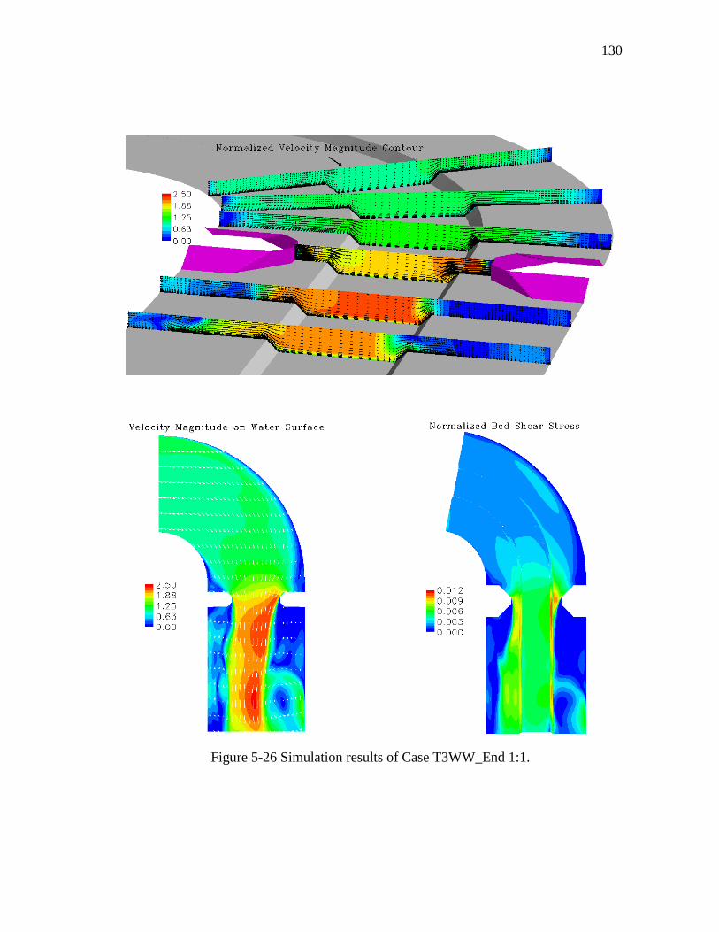
130
Figure 5-26 Simulation results of Case T3WW_End 1:1.
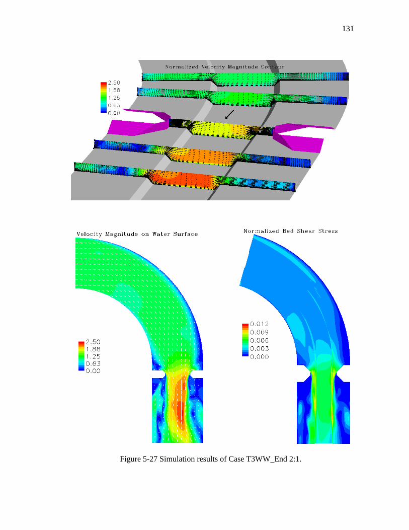
131
Figure 5-27 Simulation results of Case T3WW_End 2:1.
132
Figure 5-28 Simulation results of Case T3ST_Mid 1:1.
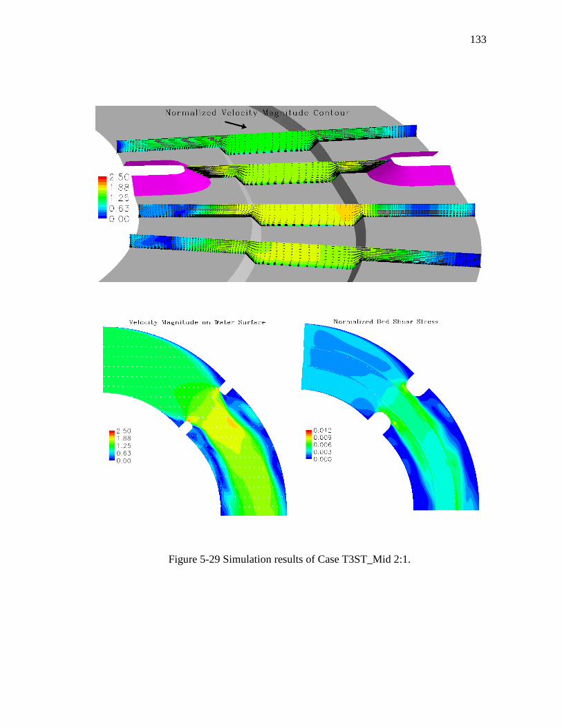
133
Figure 5-29 Simulation results of Case T3ST_Mid 2:1.
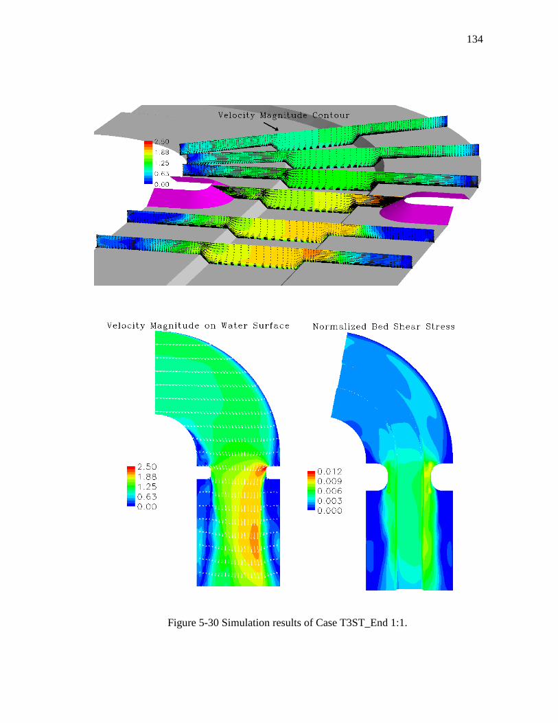
134
Figure 5-30 Simulation results of Case T3ST_End 1:1.

135
Figure 5-31 Simulation results of Case T3ST_End 2:1.
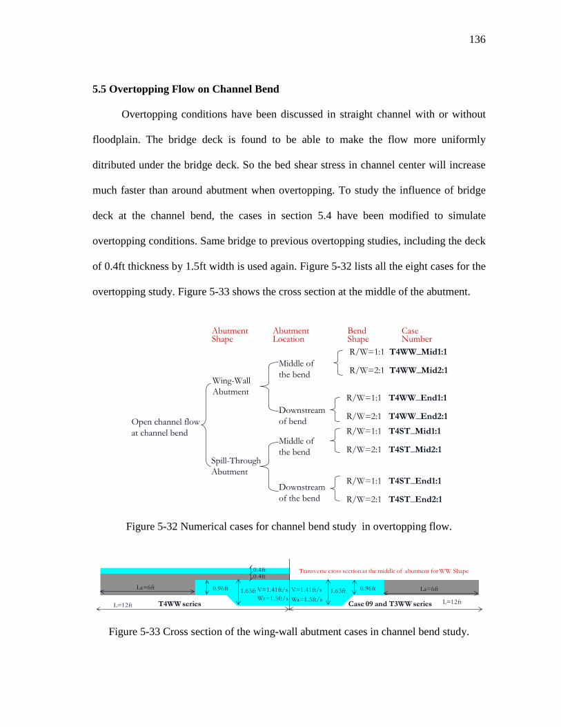
136
5.5 Overtopping Flow on Channel Bend
Overtopping conditions have been discussed in straight channel with or without
floodplain. The bridge deck is found to be able to make the flow more uniformly
ditributed under the bridge deck. So the bed shear stress in channel center will increase
much faster than around abutment when overtopping. To study the influence of bridge
deck at the channel bend, the cases in section 5.4 have been modified to simulate
overtopping conditions. Same bridge to previous overtopping studies, including the deck
of 0.4ft thickness by 1.5ft width is used again. Figure 5-32 lists all the eight cases for the
overtopping study. Figure 5-33 shows the cross section at the middle of the abutment.
Open channel flow at channel bend
Wing-Wall Abutment
Spill-Through Abutment
Middle of the bend
Downstream of the bend
Middle of the bend
Downstream of bend
R/W=1:1 T4WW_Mid1:1
R/W=2:1 T4WW_Mid2:1
R/W=1:1 T4ST_Mid1:1
R/W=2:1 T4ST_Mid2:1
R/W=1:1 T4WW_End1:1
R/W=2:1 T4WW_End2:1
R/W=1:1 T4ST_End1:1
R/W=2:1 T4ST_End2:1
AbutmentShape
AbutmentLocation
BendShape
CaseNumber
Figure 5-32 Numerical cases for channel bend study in overtopping flow.
0.96ftV=1.41ft/sV=1.41ft/sWa=1.5ft/s Wa=1.5ft/s
0.4ft0.4ft
L=12ft L=12ft
La=6ft
Case 09 and T3WW series
0.96ftLa=6ft 1.63ft1.63ft
Transverse cross section at the middle of abutment for WW Shape
T4WW series
Figure 5-33 Cross section of the wing-wall abutment cases in channel bend study.

137
5.5.1 Comparison of open channel flow to overtopping flow on channel bend
Comparing two sets of simulations on channel bends for open channel flow and
overtopping flow, the bed shear stress is found to have significant increase under
overtopping conditions. The overtopping cases has a higher channel contraction ratio
than the corresponding open channel cases. The increment of the contraction ratio is
about 6.5% and 10.5% for wing-wall and spill-through abutment respectively. Table 5-8
shows the comparison of the maximum bed shear stresses. The increment is from 32% to
90%.
open channel flow Cf_max_open Overtopping flow Cf_max_over Cf_max_over/ Cf_max_open
T3WW_Mid 1:1 0.0130 T4WW_Mid 1:1 0.0187 1.44 T3WW_Mid 2:1 0.0109 T4WW_Mid 2:1 0.0167 1.53 T3WW_End 1:1 0.0108 T4WW_End 1:1 0.0178 1.65 T3WW_End 2:1 0.0092 T4WW_End 2:1 0.0175 1.90 T3ST_Mid 1:1 0.0098 T4ST_Mid 1:1 0.0129 1.32 T3ST_Mid 2:1 0.0087 T4ST_Mid 2:1 0.0134 1.54 T3ST_End 1:1 0.0095 T4ST_End 1:1 0.0132 1.39 T3ST_End 2:1 0.0070 T4ST_End 2:1 0.0130 1.86
Table 5-8 Results under overtopping and open channel conditions.
At the upstream of the bridge, the overtopping cases have lower bed shear stresses
than the corresponding open channel flow cases in section 5.4. This is consistant to the
influence of the water depth. Generally, the bed shear stress will decrease with the
increase of the water depth. While at downstream side of the bridge, the influnce of the
bridge deck can last for a long distance. This has been observed in strainght channel
study.

138
5.5.2 Influence of R/W
The comparison will still be conducted between the two cases with wing-wall
abutment at the middle of channel bend. Comparing with the open channel flow cases,
these two overtopping cases have a significant increase on the maximum bed shear stress.
For R/W equal to 1:1, with the increase of water depth, Cf_max increases from 0.010 to
0.019. At the same time, the location of Cf_max changes from downstream main channel
slope back to upstream corner of the abutment. For R/W equal to 2:1, with the increase
of water depth, Cf_max increases from 0.011 to 0.017. The location of maximum bed shear
stress also changes back from downstream main channel slope to the upstream corner of
the abutment. The interesting finding is that the bed shear stress on the both overbank
areas under the bridge deck has a remarkable increase. And the bed shear stress in this
area is uniformly high. This is quite different from the open channel flow conditions. At
the middle of the abutment, the difference between inner and outer abutment are not big
even for R/W equal to 1:1. For the case with R/W equal to 2:1, the shear stress
distribution is almost in symmetry. The high bed shear stress at down stream inner
overbank in Case T3WW_Mid 1:1 is not observable in overtopping conditions. Overall,
the effect of bridge deck tends to decrease the effect of channel bend and make the flow
more uniform. However, the influence of the channel bend can still be found at the far
downstream outer main channel slope. Both Case T3WW_Mid 1:1 and Case
T4WW_Mid 1:1 have this feature. It is believed that the channel bend after the abutment
is responsible for the highly asymmetric result.
139
For overtopping flow, the most concerned is the flow under bridge deck since it is
highly related with the bed shear stress distribution. So the plan view of 0.5ft above the
flood plain surface is presented in the figures. For Case T4WW_Mid 1:1, the flow has
became asymmetric when approaching the abutment. The inner half channel has higher
velocity magnitude. However, at the middle of the abutment, the velocity contours are
almost symmetric. Even at the downstream side of the abutment, the velocity contour
can still keep in symmetry for some distance. The asymmetric velocity contour begins
from the end of the channel bend. This is consistent to the observation in the bed shear
stress distribution. For Case T4WW_Mid 2:1, the flow basically remains symmetric
when approaching the abutment. And this symmetric flow extends to the end of the
channel bend. At the far downstream side, the asymmetric trend begins to show up. But
it is not as serious as T4WW_Mid 1:1.
The cross section plots are also presented in figure 5-34 and figure 5-35. Same to
the straight channel, higher velocity appears on the bridge surface. And under the bridge
deck, the velocity is stratified and remains constant in the horizontal direction. The
higher velocity appears in the bottom half channel. At downstream of the bridge deck,
the surface velocity drops very quick. The higher velocity region extends far from the
bridge toward downstream.
5.5.3 Influence of abutment location
For open channel flow, the higher bed shear stress is found to be around inner
abutment when the bridge is located at the middle of the channel bend. And the inner
abutment tends to force the flow further toward outer bank. The influence of the outer

140
abutment is not obvious. However, the trend is opposite when the bridge is located at the
end of the channel bend. Higher bed shear stress is observed around the outer abutment.
And the outer abutmet tends to force the skewed flow back to the main channel and
decrease the impact of the flow on the outer overbank. The effect of inner abutment is
not obvious.
For over topping cases, the space under the deck is closed by the abutments and
the bridge deck. The flow passing through this closed sapce will be pressurized and
redistributed. At upstream side, there is no-slip boudnary only on the river bottom. The
velocity is higher at the free surface. Under the bridge deck, there is no-slip boundary for
both the top and bottom. So the flow will be squeezed to the center. The adjustment of
the flow will take place at both vertical and horizontal direction. This adjustment will
make the flow more uniformly distributed. This can be refected by the bed shear stress
contours. For all the eight simulation results shown in Figures 5-34 to 5-38, the
difference on the both sides of overbank under the bridge deck is not as large as open
channel flow cases. The influence of abutment location on the bed shear stress
distribution under bridge deck can not be observed under overtopping conditions.
At far downstream, the influence of the bridge deck is not strong. And the bend
effect retakes the domination of the flow. For the cases with abutment in the middle of
the channel bend, the asymmetric bed shear stress contours appear again. This is very
close to the distribution observed in open channel flow cases. It is believed that the
second half the channel bend after bridge causes the asymmetry of the flow. However,
this asymmetry is not found for the results with abutment at the end of the channel bend.
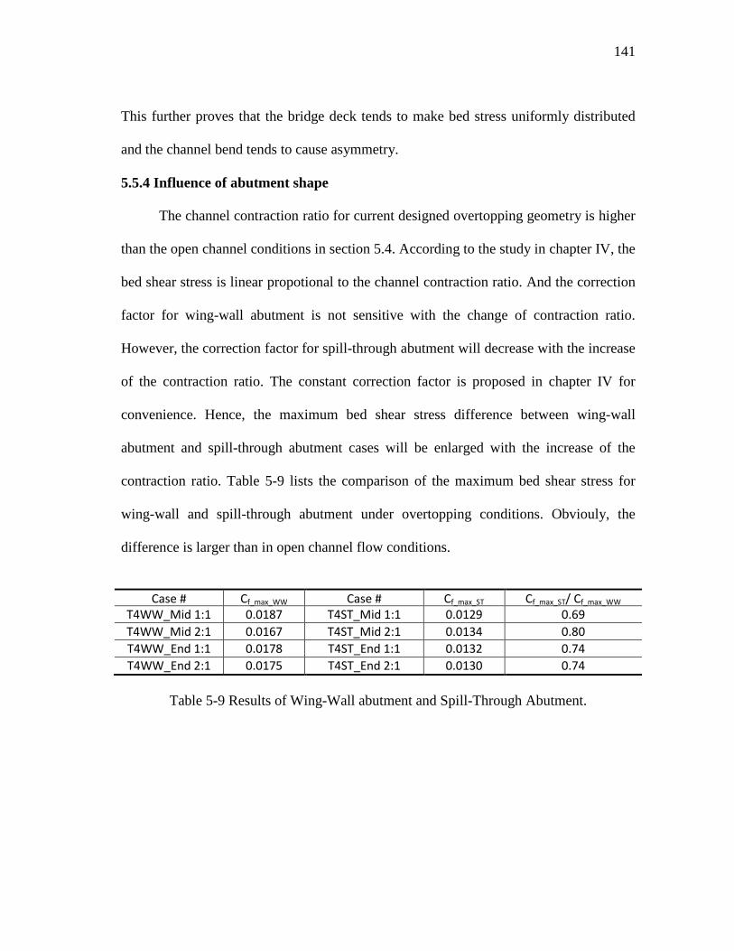
141
This further proves that the bridge deck tends to make bed stress uniformly distributed
and the channel bend tends to cause asymmetry.
5.5.4 Influence of abutment shape
The channel contraction ratio for current designed overtopping geometry is higher
than the open channel conditions in section 5.4. According to the study in chapter IV, the
bed shear stress is linear propotional to the channel contraction ratio. And the correction
factor for wing-wall abutment is not sensitive with the change of contraction ratio.
However, the correction factor for spill-through abutment will decrease with the increase
of the contraction ratio. The constant correction factor is proposed in chapter IV for
convenience. Hence, the maximum bed shear stress difference between wing-wall
abutment and spill-through abutment cases will be enlarged with the increase of the
contraction ratio. Table 5-9 lists the comparison of the maximum bed shear stress for
wing-wall and spill-through abutment under overtopping conditions. Obviouly, the
difference is larger than in open channel flow conditions.
Case # Cf_max_WW Case # Cf_max_ST Cf_max_ST/ Cf_max_WW
T4WW_Mid 1:1 0.0187 T4ST_Mid 1:1 0.0129 0.69 T4WW_Mid 2:1 0.0167 T4ST_Mid 2:1 0.0134 0.80 T4WW_End 1:1 0.0178 T4ST_End 1:1 0.0132 0.74 T4WW_End 2:1 0.0175 T4ST_End 2:1 0.0130 0.74
Table 5-9 Results of Wing-Wall abutment and Spill-Through Abutment.
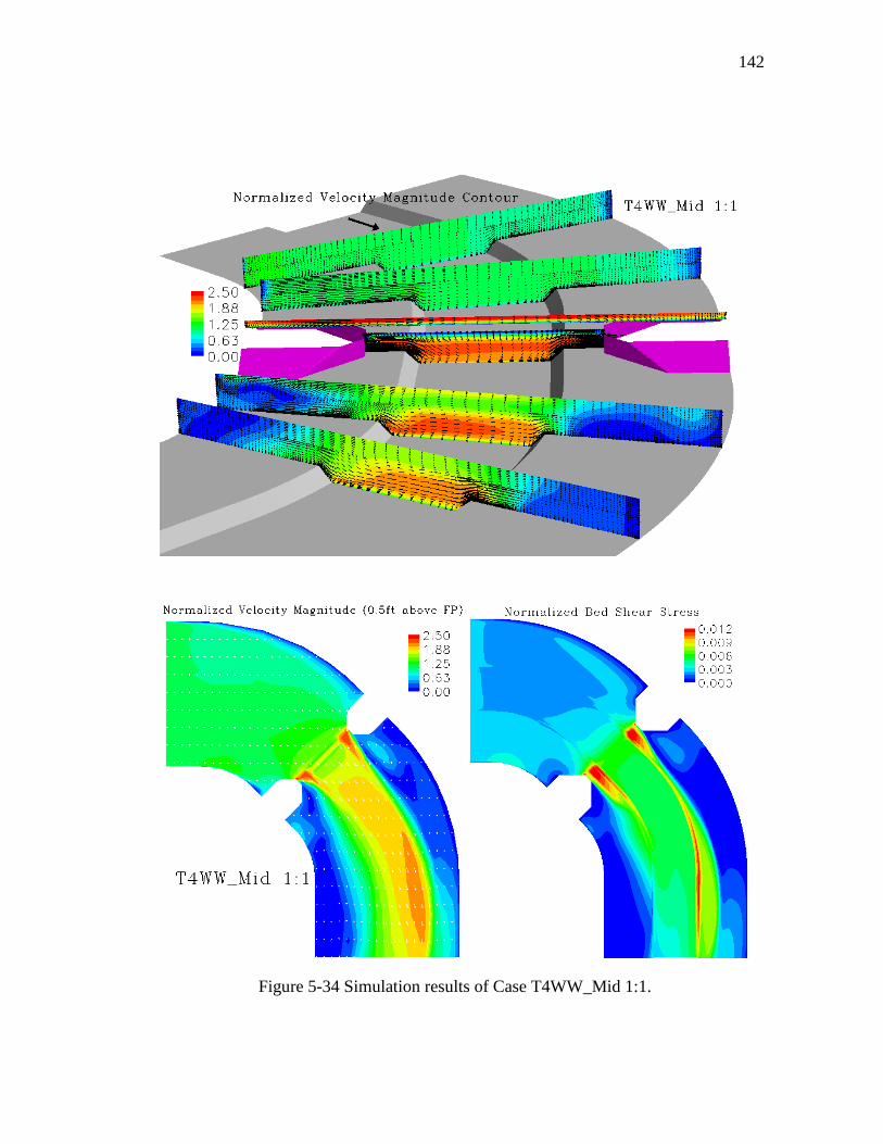
142
Figure 5-34 Simulation results of Case T4WW_Mid 1:1.

143
Figure 5-35 Simulation results of Case T4WW_Mid 2:1.
144
Figure 5-36 Simulation results of Case T4WW_End 1:1.

145
Figure 5-37 Simulation results of Case T4WW_End 2:1.

146
Figure 5-38 Normalized bed shear stress contours of the spill-through abutment cases.

147
5.6 Confluence of Tributary Upstream of a Bridge
Many situations can cause the asymmetric flow in channel. The confluence of
tributary upstream is one of those. It is simulated by modifing the flume test Case 14 to
include a tributary at upstream. The Case 14 is a symmetric channel. To simplify the
study, overtopping is not considered. In techniqe, CHEN3D program is capable to
handle the overtopping and confluence at the same time. In Case 14, the channel is
rectangular of 24ft wide; abutment is 4.33 ft long of wing-wall shape; water depth is
1.2ft; approach velocity is 1.09 ft/s. To study the non-symmetric flow, the full channel is
simulated instead of half channel as before. A tributary is added to the straight channel
24ft ahead of the abutment. The width of the tributary is 12ft. Water depth and velocity
are all same to Case 14. The tributary channel is at an angle of 30 degree from the
straight channel. Constant velocity is applied at the inlets of straight channel and the
tributary channel. The free surface is assumed to be rigid lid.
Figure 5-39 shows the velocity magnitude contours on the free surface. It is
expected to see the asymmetric contours. The shape of the contours depicts clearly the
confluence of the flow from two inlets. The flow rate from the tributary is only half of
the contribution from the straight channel. Obviously, the high flow rate component will
dominate the direction of the confluence. The asymmetric flow starts from the
confluence location and the high unit flow rate region gradually moves toward the
channel center. When passing around the abutment, the highest unit flow rate is still on
the tributary side. And the shape of the contours are quite different for two sides. The
contours are in smooth transition around the lower abutment. This indicate that the lower

148
abutment has smaller influence on the flow. On the other side, there is sharp transition
from the upstream corner of the abutment to the channel center. This shows that the
upper abutemnt impacts the skewed the flow significantly. The higherst velocity appears
at the downstream of the abutment, and the direction is relatively steady. The entire flow
field at downstream is not in symmetry. The half straight chanel with tributatry has the
higher flow rate. It is believed that the influence of upstream confluence will decrease
with the increase of the distance between tributary to abutment.
Figure 5-39 Velocity magnitude contours on the water surface.
2L=24ft
2L
V=1.09ft/s
V=1.09ft/s 2L30 °
La=3.33ft
La=3.33ftWa=1.5ft; WW abutment
2L=24ft2L=24ft
2L2L
V=1.09ft/s
V=1.09ft/s 2L30 °
La=3.33ftLa=3.33ft
La=3.33ftLa=3.33ftWa=1.5ft; WW abutment
Figure 5-40 Normalized bed shear stress contours.
Figure 5-40 shows the bed shear stress contours. The pattern at upstream is very
similar to the velocity magnitude contours on water surface. The bed shear stress is also
149
asymmetric. At upstream side, the high bed shear stress region start from the confluence
location and skewed to the opposite abutment. The maximum bed shear stress appears at
the abutment opposite to the tributary channel. At the downstream side, the bed shear
stress contour skews back to the side of the tributary channel.

150
CHAPTER VI
ABUTMENT SCOUR IN COHESIVE SOILS
The main purpose of this section is to study scour model in cohesive soils and
simulate the flume test cases in NCHRP 24-15(2). The numerical method described in
chapter III has been applied to perform the simulations. There are two steps in scour
prediction; first step is to establish the initial flow field without scour development; the
second step is to simulate the scour process based on the scour model embedded in
CHEN3D code. The second purpose of this section is to study the influence of
overtopping flow on scour process in cohesive soils. Correction factors for overtopping
flow have been proposed based on the numerical studies.
6.1 Soil Properties
Porcelain clay was used in the flume tests of NCHRP 24-15(2). Geotechnical tests
were performed according to ASTM standards. The results of two testing have been
tabulated in table 6-1. Erosion properties of the porcelain clay were tested through EFA
(Erosion Function Apparatus). Eleven EFA testing were performed using tap water.
These samples were from different testing conditions. The first testing was conducted
with the fresh sample which should represent most of the clay used in the flume tests.
The regression curve in figure 6-1 is based on the first EFA testing, which is used as the
erosion function of the soils in all the numerical simulations of scour prediction. There
were several samples taken from the clay stored for a long time or the leftover after the
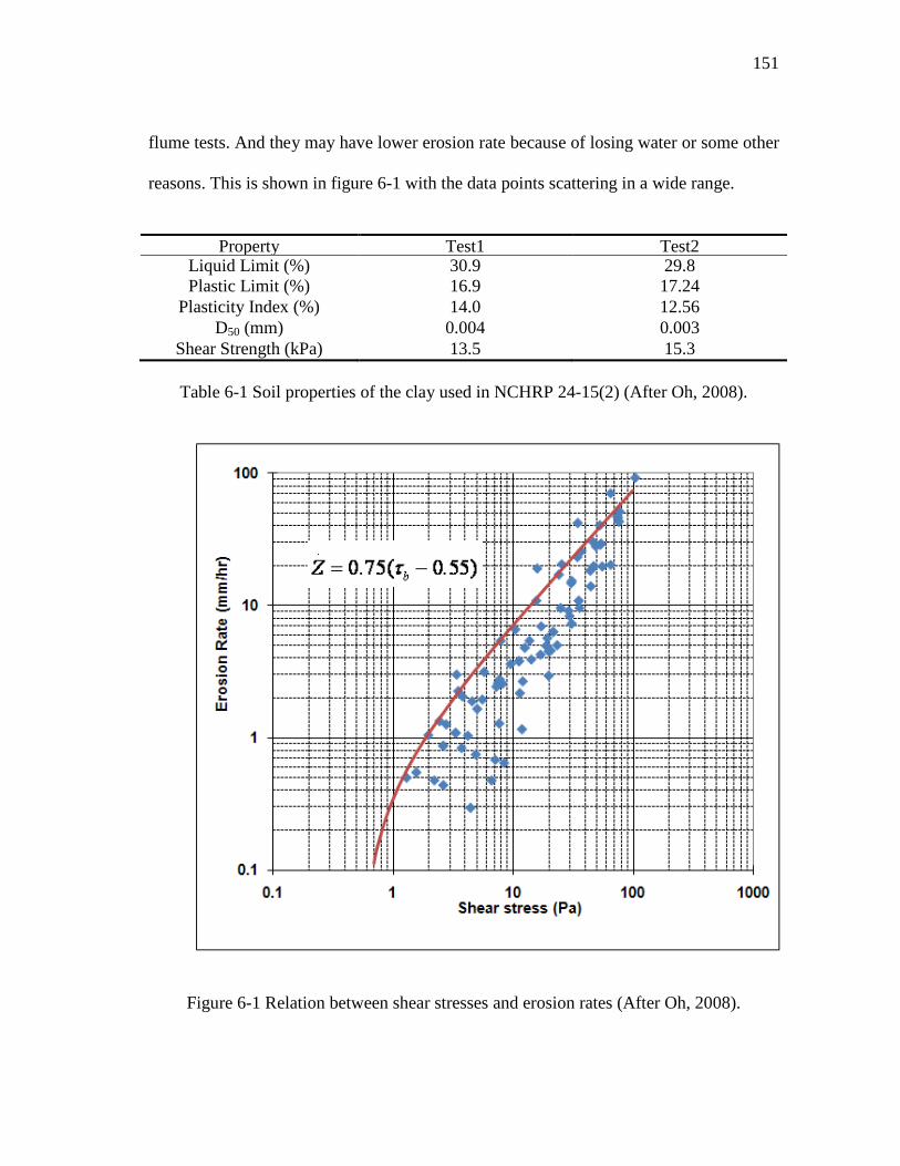
151
flume tests. And they may have lower erosion rate because of losing water or some other
reasons. This is shown in figure 6-1 with the data points scattering in a wide range.
Property Test1 Test2
Liquid Limit (%) 30.9 29.8 Plastic Limit (%) 16.9 17.24
Plasticity Index (%) 14.0 12.56 D50 (mm) 0.004 0.003
Shear Strength (kPa) 13.5 15.3
Table 6-1 Soil properties of the clay used in NCHRP 24-15(2) (After Oh, 2008).
Figure 6-1 Relation between shear stresses and erosion rates (After Oh, 2008).
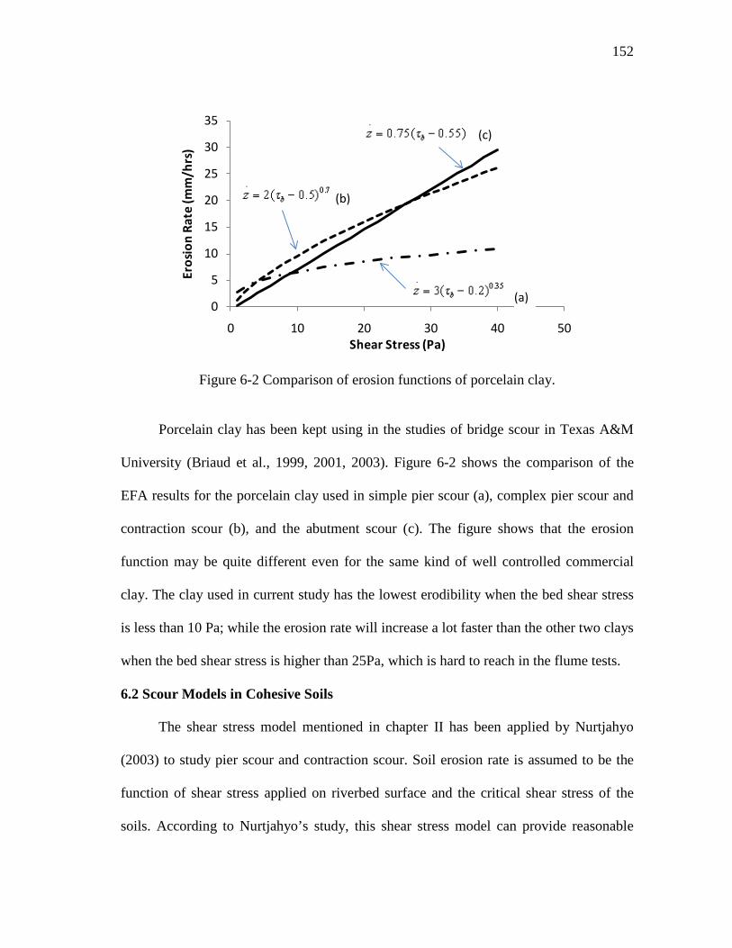
152
0
5
10
15
20
25
30
35
0 10 20 30 40 50
Eros
ion
Rate
(mm
/hrs
)
Shear Stress (Pa)
Figure 6-2 Comparison of erosion functions of porcelain clay.
Porcelain clay has been kept using in the studies of bridge scour in Texas A&M
University (Briaud et al., 1999, 2001, 2003). Figure 6-2 shows the comparison of the
EFA results for the porcelain clay used in simple pier scour (a), complex pier scour and
contraction scour (b), and the abutment scour (c). The figure shows that the erosion
function may be quite different even for the same kind of well controlled commercial
clay. The clay used in current study has the lowest erodibility when the bed shear stress
is less than 10 Pa; while the erosion rate will increase a lot faster than the other two clays
when the bed shear stress is higher than 25Pa, which is hard to reach in the flume tests.
6.2 Scour Models in Cohesive Soils
The shear stress model mentioned in chapter II has been applied by Nurtjahyo
(2003) to study pier scour and contraction scour. Soil erosion rate is assumed to be the
function of shear stress applied on riverbed surface and the critical shear stress of the
soils. According to Nurtjahyo’s study, this shear stress model can provide reasonable
(a)
(b)
(c)
153
prediction for the deepest scour depth. However, the scour pattern is not in good
agreement with the measurement. For example, in pier scour study, the maximum bed
shear stress appears only in front of pier facing the flow where the flow is mostly
accelerated. While in the wake region behind the pier, the bed shear stress is very low.
Hence, the deepest scour hole can only be generated in front of the pier based on shear
stress model. Actually, deep scour occurs at both upstream and downstream sides of the
pier, where the magnitudes of the scour depths are similar in most cases. This indicates
that bed shear stress is not the only contributor to the development of scour hole around
hydraulic structure. A promising assumption has been proposed in Nurtjahyo’s
dissertation, which says that the turbulence could affect the scour development and its
contribution might be as same as bed shear stress. Nurtjahyo further proposed a scour
model including the shear stress and turbulent kinetic energy and performed the
numerical studies with the new scour model. The maximum value of turbulent kinetic
energy in the vertical direction above the bed at about 10% of water depth was used in
the simulations. According to his study, the new model could generate deep scour hole at
both upstream and downstream sides of pier, which is consistent to the finding in
experiments. The scour model proposed by Nurtjahyo (2003) is as follows:
. .
( , , ) ( )= = − + ⋅b c b cz z k c b kτ τ τ τ (6.1)
Where, .z is the erosion rate (mm/hour); bτ is the bed shear stress (Pa); cτ is the
critical shear stress of the soils (Pa); c is the slope of erosion rate versus shear stress
curve (m3/(N·hr); k is turbulent kinetic energy (m/s)2 and b is the constant (s/m).

154
In Nurtjahyo’s study, the hydraulic smooth boundary condition has been applied
throughout all the simulations. The influence of the surface roughness has been
discussed in chapter V. In the verification case of overtopping, there is no scour during
the testing and the roughness of the river bottom is constant. The bed shear stress in the
roughened channel is amplified significantly compared to the result in the hydraulic
smooth channel. As for clay, the soil particles are extremely fine, and the flat surface
without scouring can definitely be taken as smooth. However, this is only suitable for the
initial conditions of flume test. When scour developing, the surface of the channel
bottom is no longer flat. This non smooth surface observed in cohesive soil channel is
somehow similar to the bed form configuration on sand beds. And this is not believed to
be able to predict with the roughness model used in chapter V since it is hard to
determine the equivalent roughness of the bed form. To compensate the bed form effect,
the correct factor β is used to augment the directly calculated bed shear stress from
CHEN3D (with hydraulic smooth surface boundary conditions). Then, the shear stress
model will be modified to be:
. .
( , , ) ( )= = − + ⋅b c num cz z k c b kτ τ βτ τ (6.2)
To determine the unknown parameters of β and b, the trial and error method has
been used. As mentioned above, the shear stress is believed to be the dominant
parameters in scour processing. Hence, the erosion function from EFA testing was
trialed first with original shear stress model of 0.75 /c mm hour= , 0.55 Pacτ = , 1.0β = ,
and 0.0=b ( called Model I ). According to the trials, the predicted scour depth is
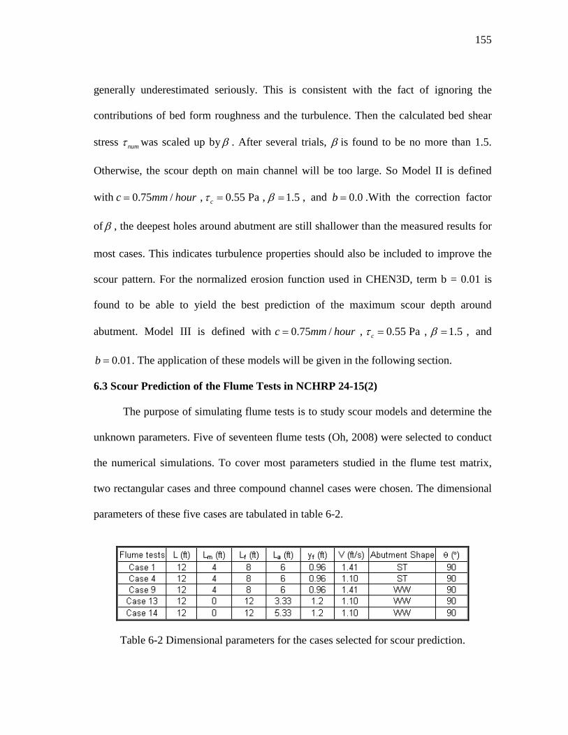
155
generally underestimated seriously. This is consistent with the fact of ignoring the
contributions of bed form roughness and the turbulence. Then the calculated bed shear
stress numτ was scaled up byβ . After several trials, β is found to be no more than 1.5.
Otherwise, the scour depth on main channel will be too large. So Model II is defined
with 0.75 /c mm hour= , 0.55 Pacτ = , 1.5=β , and 0.0=b .With the correction factor
of β , the deepest holes around abutment are still shallower than the measured results for
most cases. This indicates turbulence properties should also be included to improve the
scour pattern. For the normalized erosion function used in CHEN3D, term b = 0.01 is
found to be able to yield the best prediction of the maximum scour depth around
abutment. Model III is defined with 0.75 /c mm hour= , 0.55 Pacτ = , 1.5=β , and
0.01=b . The application of these models will be given in the following section.
6.3 Scour Prediction of the Flume Tests in NCHRP 24-15(2)
The purpose of simulating flume tests is to study scour models and determine the
unknown parameters. Five of seventeen flume tests (Oh, 2008) were selected to conduct
the numerical simulations. To cover most parameters studied in the flume test matrix,
two rectangular cases and three compound channel cases were chosen. The dimensional
parameters of these five cases are tabulated in table 6-2.
Table 6-2 Dimensional parameters for the cases selected for scour prediction.
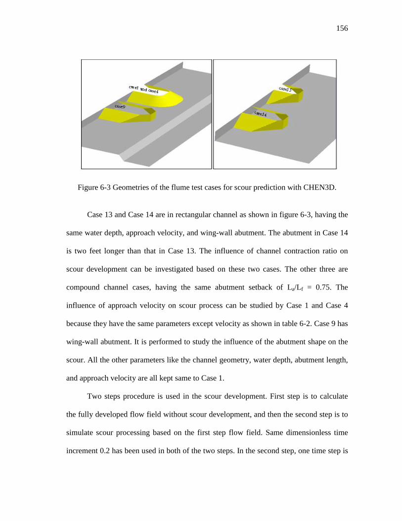
156
Figure 6-3 Geometries of the flume test cases for scour prediction with CHEN3D.
Case 13 and Case 14 are in rectangular channel as shown in figure 6-3, having the
same water depth, approach velocity, and wing-wall abutment. The abutment in Case 14
is two feet longer than that in Case 13. The influence of channel contraction ratio on
scour development can be investigated based on these two cases. The other three are
compound channel cases, having the same abutment setback of La/Lf = 0.75. The
influence of approach velocity on scour process can be studied by Case 1 and Case 4
because they have the same parameters except velocity as shown in table 6-2. Case 9 has
wing-wall abutment. It is performed to study the influence of the abutment shape on the
scour. All the other parameters like the channel geometry, water depth, abutment length,
and approach velocity are all kept same to Case 1.
Two steps procedure is used in the scour development. First step is to calculate
the fully developed flow field without scour development, and then the second step is to
simulate scour processing based on the first step flow field. Same dimensionless time
increment 0.2 has been used in both of the two steps. In the second step, one time step is
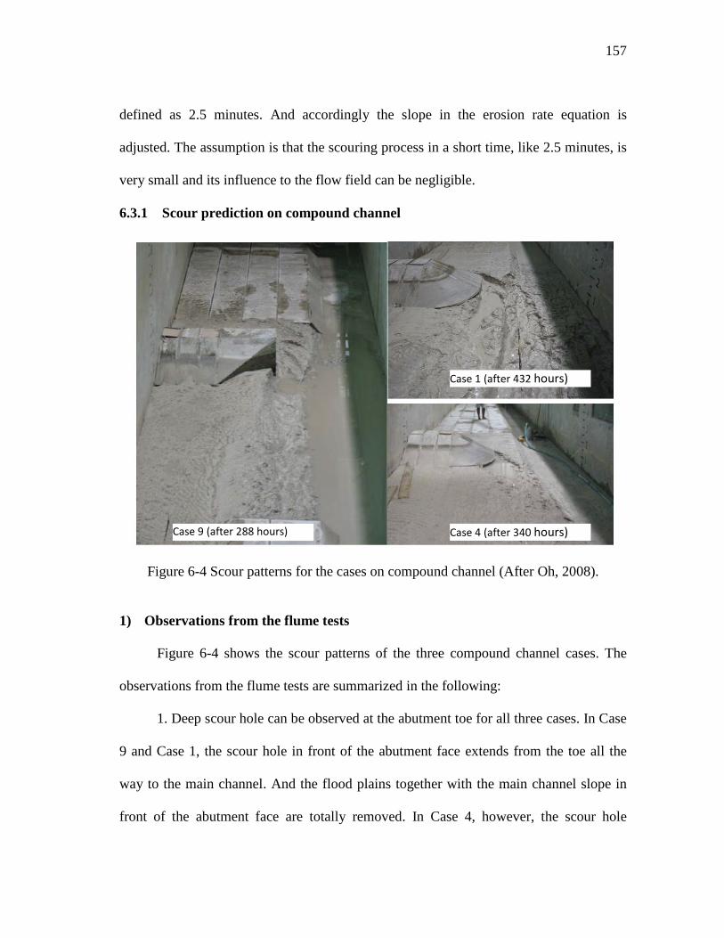
157
defined as 2.5 minutes. And accordingly the slope in the erosion rate equation is
adjusted. The assumption is that the scouring process in a short time, like 2.5 minutes, is
very small and its influence to the flow field can be negligible.
6.3.1 Scour prediction on compound channel
Figure 6-4 Scour patterns for the cases on compound channel (After Oh, 2008).
1) Observations from the flume tests
Figure 6-4 shows the scour patterns of the three compound channel cases. The
observations from the flume tests are summarized in the following:
1. Deep scour hole can be observed at the abutment toe for all three cases. In Case
9 and Case 1, the scour hole in front of the abutment face extends from the toe all the
way to the main channel. And the flood plains together with the main channel slope in
front of the abutment face are totally removed. In Case 4, however, the scour hole
Case 1 (after 432 hours)
Case 9 (after 288 hours) Case 4 (after 340 hours)
158
around that abutment toe is limited on the flood plain and the main channel slope
including part of the flood plain is still remained after two weeks’ scouring.
2. At the downstream side, the original main channel slope was completely
washed away for Case 1 and Case 9 after the testing. And the bottom was eroded to the
same level as the main channel or even lower for Case 1. The main channel slope
regresses toward the over bank to the location in line with the abutment toe. As for Case
4, the erosion of the original main channel slope was not very serious. The scour hole
started from the upstream corner of the abutment and extended toward downstream main
channel slope, which shows the skewed flow stream lines forced by the abutment.
However, this trend is not observed in Case 1 and Case 9 when the approach velocity is
higher.
3. The surface of the channel bottom after scouring is not as smooth as the initial
conditions. In the region without obvious erosion, like the upstream part far from the
abutment and the flood plain behind the abutment at downstream, the surface is still flat.
As for the region with serious erosion, the bed surface is highly uneven.
4. Main channel has much smaller scour depth than main channel slope and flood
plain. The scour hole on the main channel slope can be as deep as the hole at the
abutment toe.
2) Simulation result and analysis of Case 9
Figure 6-5 shows the plan view of the measured and simulated scour patterns of
Case 9 after 240 hours. The comparison of three scour models will be conducted one by
one in the following:

159
Compare to the measurement, Model I generated smaller eroded area, which
indicates the calculated bed shear stress is less than the real bed shear stress applied by
the flow. As mentioned before, this difference might result from the effect of bed form
roughness. Turbulence should not relate with this issue since it contributes only the
specific area and will not affect the main channel much. The deepest scour hole with
model I is on the main channel slope with the depth of 0.4ft, which is about half of the
measured deepest scour depth. However, the deepest scour hole observed in the flume
test is at the downstream corner of the abutment, which could not be observed from this
simulation.
Model II shows similar eroded area to the measurement. In most area, the
simulated scour depth is in good agreement with the measurement, especially for the
contraction scour in main channel. This proves that the bed form roughness should be
considered in scour model. However, the deepest scour depth, mostly concerned in
bridge design, could not be matched by scaling up the calculated bed shear stress
uniformly.
For model III, the plan view shows that the scour pattern can be improved
compared with model 1 and model 2. The deep scour holes can be found in front of
abutment face and on main channel slope. And the magnitude of the maximum abutment
scour depth is very close to the measurement. However, the kinetic energy model
contributes to not only the scour around abutment but also the scour in the main channel.
It makes the scour prediction on the main channel higher than the measurement. Hence,
the turbulence term in the model still needs to be further studied.

160
X (ft)
Y(ft
)
-5 0 5 10 150
6
12
0.80.70.60.50.40.30.20.1
Scour depth contour (ft); Flume test Case9
X (ft)
Y(ft
)
-5 0 5 10 15 200
6
12
0.80.70.60.50.40.30.20.1
Scour depth contour (ft); Simulation Case 9 (Model III)
X (ft)
Y(ft
)
-5 0 5 10 15 200
6
12
0.80.70.60.50.40.30.20.1
Scour depth contour (ft); Simulation Case 9 (Model II)
X (ft)
Y(ft
)
-5 0 5 10 15 200
6
12
0.80.70.60.50.40.30.20.1
Scour depth contour (ft); Simulation Case 9 (Model I)
Figure 6-5 Scour depths after 10 days for different scour models (Case 9).

161
-10
-8
-6
-4
-2
0
2
0 2 4 6 8 10 12
Scou
r D
epth
(inc
h)
T Station (ft)
Scour Depth Profile at Middle of Abutment
Measurement
Model I
Model II
Model III
-10
-8
-6
-4
-2
0
2
0 2 4 6 8 10 12
Scou
r D
epth
(inc
h)
T Station (ft)
Scour Depth Profile at upstream of Abutment
Measurement
Model I
Model II
Model III
-10
-8
-6
-4
-2
0
2
0 2 4 6 8 10 12
Scou
r D
epth
(inc
h)
T Station (ft)
Scour Depth Profile at downstream of Abutment
Measurement
Model I
Model II
Model III
Figure 6-6 Scour profiles for Case 9 after 10 days at different cross sections.
162
Figure 6-6 shows the comparison of the predicted scour depth profile to the
measurement at different cross sections. These three cross sections were selected around
the abutment at upstream side, in the middle, and at downstream side of the abutment.
The deepest scour may occur at other locations. However, the scour pattern around
abutment is most concerned in the engineering practice.
At upstream side of the abutment, the flow starts to accelerate at the opening part
of the channel and slow down at the region blocked by the abutment. The measured
scour depth in the opening part from T station 6ft to 12 ft is about 2inches. Actually, the
erosion begins from 4.5 ft where the flow begins to be squeezed into the unblocked area.
Model I underestimates the scour depth along the entire cross section. Prediction of
model II is very close to the measurement. And Model III predicts higher scour depth in
most area. But both model II and model III can reflect the trend correctly at upstream.
In the middle of the abutment, the measured scour depth is about 8 inches at the
abutment toe and about 3 inches on the main channel. It should be noted that the scour is
deep on location of main channel slope from T station 8ft to 8.67 ft, which is consistent
with the bed shear stress trend. Model I still underestimates the scour depth. Model II
yields good prediction in most part except at abutment toe. For model III, the predicted
scour depth increases entirely across the channel. The advantage is that the kinetic
energy term can generate the deep scour hole at the abutment toe.
At downstream side of the abutment, the measured scour depth behind the
abutment from 0ft to 6ft is negligible. The deepest hole appears on the main channel
slope of 8 inches. The contracted scour depth on the main channel is about 4 inches. All

163
three models can predict trend correctly. And the best agreement is given by scour model
II.
0
50
100
150
200
250
300
0 40 80 120 160 200 240
T ime (hours)
Max
. S
cou
r D
epth
(mm
) Meas urementModel IModel IIModel III
Figure 6-7 Maximum scour depths history for Case 9.
Usually, the most concerned is the deepest scour depth, which is needed in the
bridge design and analysis. All the abutment scour equations listed in HEC-18 intend to
predict only the value of Zmax and have nothing to do with the scour pattern. Hence it is
necessary to study Zmax as well as studying the scour pattern. Figure 6-7 presents the
comparison of the simulated Zmax over time based on different scour models. The Zmax in
figure 6-7 is the deepest scour depth at each time instant; the location of Zmax is not
constant over time. For Case 9, the deepest hole is always in front of the abutment face
according to the flume test, although the scour on the main channel slope is also very
deep. As expected, the model with the correction of bed form roughness and kinetic
energy could match the measurement very well in the point of Zmax.

164
3) Simulation result and analysis of Case 1
Figure 6-8 shows the scour profiles at same three cross sections. The trends of the
simulation results are basically similar to the measurements. Model I underestimates the
scour depth at all three cross sections. Model II could generate closer prediction to the
measurements at upstream and in the middle of the abutment. This time, the deep scour
depth at the abutment toe can be observed from the simulation. However, the scour hole
on the main channel slope could not be captured clearly. At downstream side, model II
yields similar trend to the measurement. But the magnitude is a lot lower. Model III, in
this case, increases the scour depth in the entire opening part and has little improvement
on the scour pattern. This can only provides better prediction on the flood plain at the
downstream cross section. But, the prediction on the main channel is much larger than
the measurement. Overall, the simulated scour depths for Case 1 are smaller than the
predicted in Case 9. This is consistent with the widely accepted conclusion that wing-
wall abutment can generate deeper scour depth than spill-through abutment. CHEN3D
simulation could reflect this trend very well.
It should be noted that the profile at the downstream part for Case 1 is very
strange. The scour hole on the main channel slope is as deep as 13 inches. While the
deepest hole at abutment toe is only about 5 inches. The deep hole may come from the
non uniform of the soil properties and the testing setup. The porcelain clay used in the
flume test may not be in the same batch. So the erosion properties may not be consistent
like discussed in the soil properties section. And during the experiment setup, the
compaction may also cause problem. There is the possibility that the downstream main
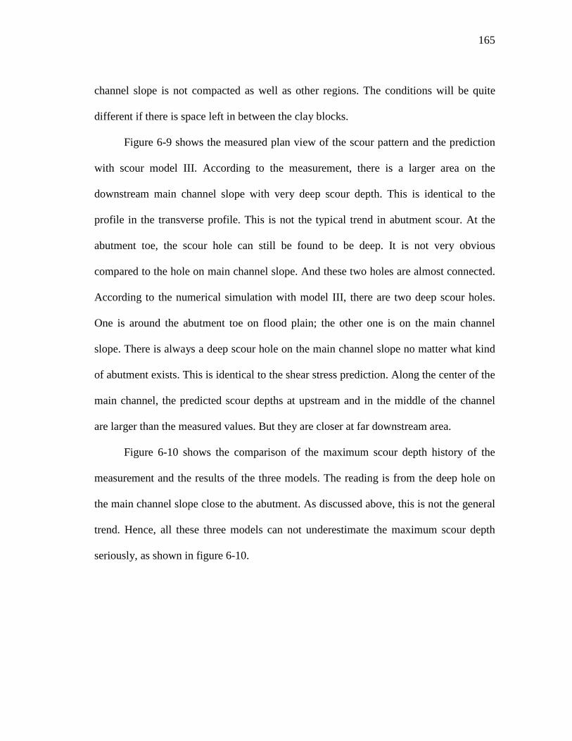
165
channel slope is not compacted as well as other regions. The conditions will be quite
different if there is space left in between the clay blocks.
Figure 6-9 shows the measured plan view of the scour pattern and the prediction
with scour model III. According to the measurement, there is a larger area on the
downstream main channel slope with very deep scour depth. This is identical to the
profile in the transverse profile. This is not the typical trend in abutment scour. At the
abutment toe, the scour hole can still be found to be deep. It is not very obvious
compared to the hole on main channel slope. And these two holes are almost connected.
According to the numerical simulation with model III, there are two deep scour holes.
One is around the abutment toe on flood plain; the other one is on the main channel
slope. There is always a deep scour hole on the main channel slope no matter what kind
of abutment exists. This is identical to the shear stress prediction. Along the center of the
main channel, the predicted scour depths at upstream and in the middle of the channel
are larger than the measured values. But they are closer at far downstream area.
Figure 6-10 shows the comparison of the maximum scour depth history of the
measurement and the results of the three models. The reading is from the deep hole on
the main channel slope close to the abutment. As discussed above, this is not the general
trend. Hence, all these three models can not underestimate the maximum scour depth
seriously, as shown in figure 6-10.

166
S c our D epth P rofile at Middle of Abutment
-14
-12
-10
-8
-6
-4
-2
0
2
0 2 4 6 8 10 12
T S ta tion (ft)
Sco
ur
Dep
th (
inch
)
Meas urem ent
Model I
Model II
Model III
S c our D epth P rofile at ups tream of Abutment
-14
-12
-10
-8
-6
-4
-2
0
2
0 2 4 6 8 10 12
T S ta tion (ft)
Sco
ur
Dep
th (
inch
)
Meas urem ent
Model I
Model II
Model III
S c our D epth P rofile at downs tream of Abutment
-14
-12
-10
-8
-6
-4
-2
0
2
0 2 4 6 8 10 12
T S ta tion (ft)
Sco
ur
Dep
th (
inch
)
Meas urem ent
Model I
Model II
Model III
Figure 6-8 Scour profiles for Case 1 after 10 days at different cross sections.
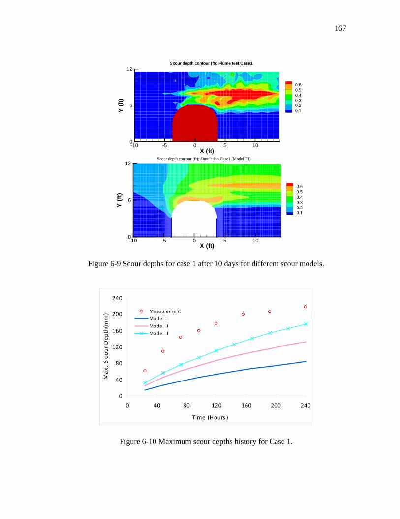
167
X (ft)
Y(ft
)
-10 -5 0 5 100
6
12
0.60.50.40.30.20.1
Scour depth contour (ft); Flume test Case1
X (ft)
Y(ft
)
-10 -5 0 5 100
6
12
0.60.50.40.30.20.1
Scour depth contour (ft); Simulation Case1 (Model III)
Figure 6-9 Scour depths for case 1 after 10 days for different scour models.
0
40
80
120
160
200
240
0 40 80 120 160 200 240
Time (Hours )
Max
. S
cour
Dep
th(m
m) Mea surement
Model I
Model II
Model III
Figure 6-10 Maximum scour depths history for Case 1.

168
4) Simulation result and analysis of Case 4
Figure 6-11 shows the scour profiles of Case 4. Case 4 has lower approach
velocity than Case 1 and Case 9. According to figure 6-11, scour depths for both the
numerical simulations and the measurements are smaller than the corresponding
conditions in Case 1. This is consistent with the influence of the velocity. At the
upstream side, all three scour models underestimates scour depth. This is opposite to the
finding in Case 9 and Case 1. In the middle of the abutment, all these three scour models
can predict the deep scour hole at abutment toe. But the predicted scour depths on main
channel are quite different from each other. Actually, the measured scour depths on main
channel for upstream and middle of the abutment are very close. It indicates the
abutment on flood plain has little influence on main channel. At downstream, both scour
model I and II can predict close result to the flume test. Scour model II can be closer on
the main channel. Scour III can match the deepest scour hole very well. But the
prediction on the main channel is too large.
Figure 6-12 shows the comparison of the plan views of the measured and
simulated scour pattern. The scour model predicted two scour holes at the abutment toe
and on the downstream main channel slope. In the flume tests, there are deep scour holes
observed at the same locations. However, the eroded area from the prediction is much
larger than the measurement.
Figure 6-13 presents the comparison of the maximum scour depth history. The
Zmax can be predicted very well with scour model III.

169
S c our Depth P rofile at Middle of Abutment
-5
-4
-3
-2
-1
0
1
0 2 4 6 8 10 12
T S ta tion (ft)
Sco
ur
Dep
th (
inch
)
Meas urem entModel IModel IIModel III
S c our Depth P rofile at ups tream of Abutment
-5
-4
-3
-2
-1
0
1
0 2 4 6 8 10 12
T S ta tion (ft)
Sco
ur
Dep
th (
inch
)
Meas urem entModel IModel IIModel III
S c our Depth P rofile at downs tream of Abutment
-5
-4
-3
-2
-1
0
1
0 2 4 6 8 10 12
T S T a tion (ft)
Sco
ur
Dep
th (
inch
)
Meas urem entModel IModel IIModel III
Figure 6-11 Scour profiles for Case 4 after 9 days at different cross sections.
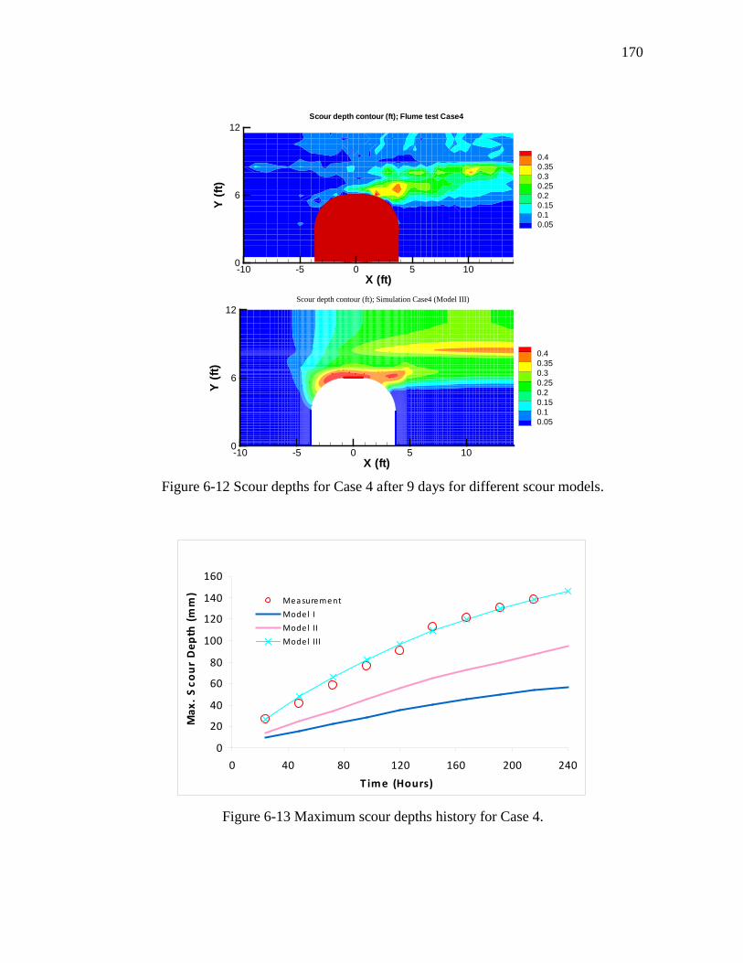
170
X (ft)
Y(ft
)
-10 -5 0 5 100
6
12
0.40.350.30.250.20.150.10.05
Scour depth contour (ft); Flume test Case4
X (ft)
Y(ft
)
-10 -5 0 5 100
6
12
0.40.350.30.250.20.150.10.05
Scour depth contour (ft); Simulation Case4 (Model III)
Figure 6-12 Scour depths for Case 4 after 9 days for different scour models.
0
20
40
60
80
100
120
140
160
0 40 80 120 160 200 240
T ime (Hours)
Max
. S
cou
r D
epth
(m
m)
Mea surement
Model I
Model II
Model III
Figure 6-13 Maximum scour depths history for Case 4.
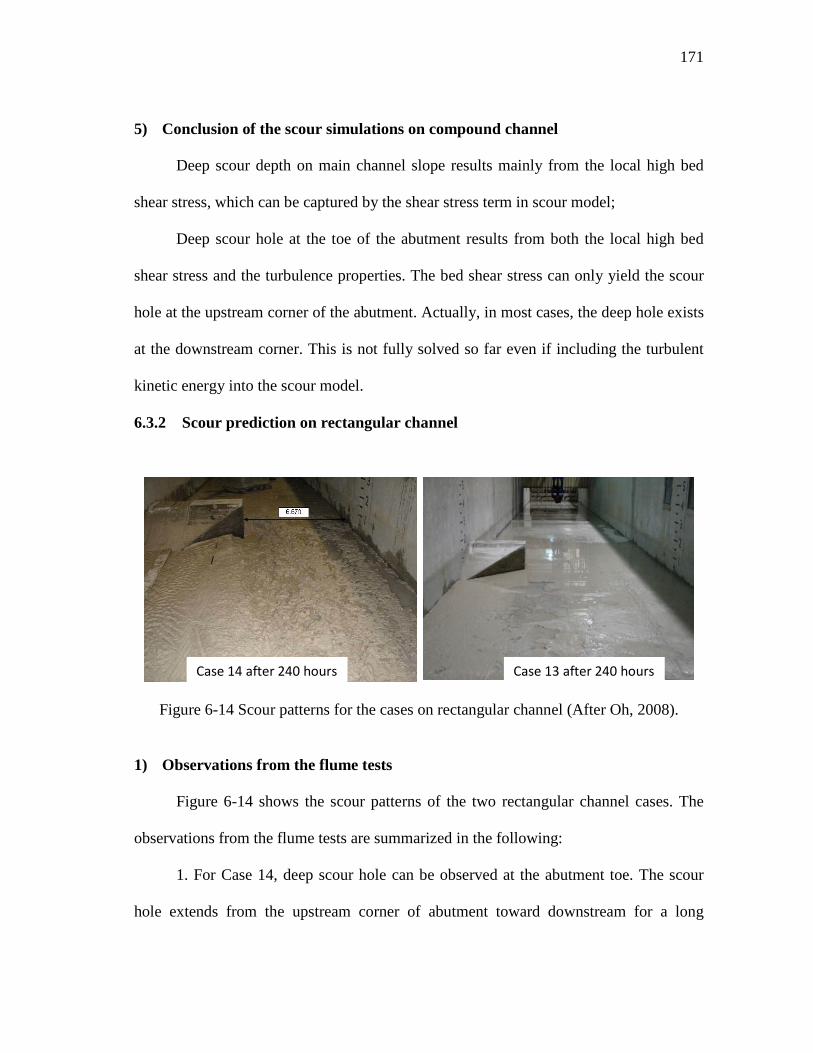
171
5) Conclusion of the scour simulations on compound channel
Deep scour depth on main channel slope results mainly from the local high bed
shear stress, which can be captured by the shear stress term in scour model;
Deep scour hole at the toe of the abutment results from both the local high bed
shear stress and the turbulence properties. The bed shear stress can only yield the scour
hole at the upstream corner of the abutment. Actually, in most cases, the deep hole exists
at the downstream corner. This is not fully solved so far even if including the turbulent
kinetic energy into the scour model.
6.3.2 Scour prediction on rectangular channel
Figure 6-14 Scour patterns for the cases on rectangular channel (After Oh, 2008).
1) Observations from the flume tests
Figure 6-14 shows the scour patterns of the two rectangular channel cases. The
observations from the flume tests are summarized in the following:
1. For Case 14, deep scour hole can be observed at the abutment toe. The scour
hole extends from the upstream corner of abutment toward downstream for a long
Case 14 after 240 hours Case 13 after 240 hours

172
distance. The scour depth along the channel center is smaller than the scour hole around
the abutment. The bed surface after scouring is uneven as shown in the picture.
2. For Case 13, the scour hole is shallower at the toe of the abutment than at
downstream. However, this is not believed to be normal and repeatable. Many reasons
can cause this problem, like bad compaction and non uniform clay. Contrary to the other
cases, the bed surface of Case 13 is still very smooth after the testing.
2) Simulation result and analysis of Case 14
Figure 6-15 shows the scour depth profiles. At upstream side, the scour depth is
very uniform, about 0.7 inches in the open area. In the middle of the abutment, the scour
depth at the channel center is about 2 inches. The scour hole is as deep as 7.5 inches
around the toe of abutment. At downstream, the scour depth at channel center is about
2.5 inches. And the deep hole extends downstream in line with abutment toe. The
blockage effect of abutment on the contraction scour is clearly observed according to the
scour depth variation along the channel center. The deepest contraction scour depth
occurs at the downstream instead of the middle of the abutment. This shows the delay of
the flow contraction against the channel contraction. The contracted scour depth is
predicted well by scour model I in the profiles. However, around the abutment toe and at
the wake region, the model has to be modified so that the prediction can match the
measurement. Scour model II and III can get closer scour depth to the measurement
around the abutment. But they overestimate the contraction seriously. The corrections of
roughness and turbulent properties are required in theory. However, further research
need to be conducted to study how the scour model should be constructed to represent
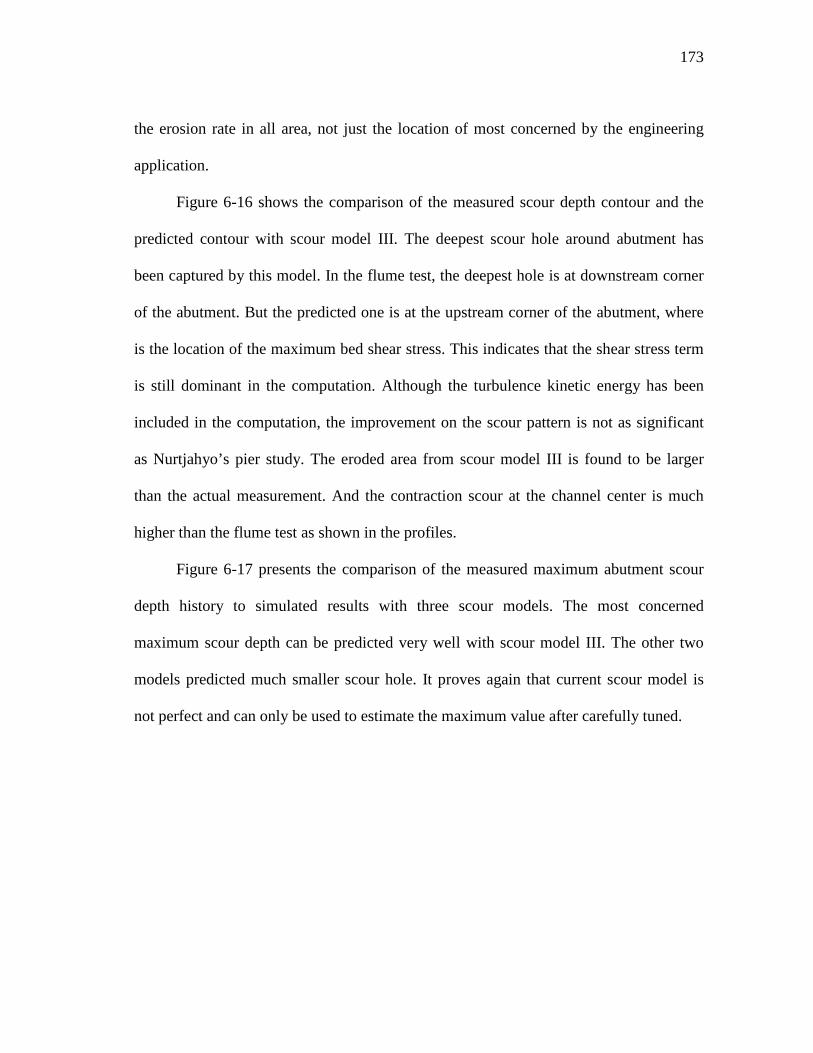
173
the erosion rate in all area, not just the location of most concerned by the engineering
application.
Figure 6-16 shows the comparison of the measured scour depth contour and the
predicted contour with scour model III. The deepest scour hole around abutment has
been captured by this model. In the flume test, the deepest hole is at downstream corner
of the abutment. But the predicted one is at the upstream corner of the abutment, where
is the location of the maximum bed shear stress. This indicates that the shear stress term
is still dominant in the computation. Although the turbulence kinetic energy has been
included in the computation, the improvement on the scour pattern is not as significant
as Nurtjahyo’s pier study. The eroded area from scour model III is found to be larger
than the actual measurement. And the contraction scour at the channel center is much
higher than the flume test as shown in the profiles.
Figure 6-17 presents the comparison of the measured maximum abutment scour
depth history to simulated results with three scour models. The most concerned
maximum scour depth can be predicted very well with scour model III. The other two
models predicted much smaller scour hole. It proves again that current scour model is
not perfect and can only be used to estimate the maximum value after carefully tuned.
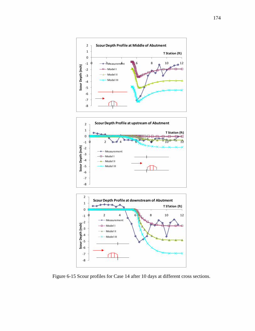
174
-8
-7
-6
-5
-4
-3
-2
-1
0
1
2
0 2 4 6 8 10 12
Scou
r D
epth
(inc
h)
T Station (ft)
Scour Depth Profile at Middle of Abutment
Measurement
Model I
Model II
Model III
-8
-7
-6
-5
-4
-3
-2
-1
0
1
2
0 2 4 6 8 10 12
Scou
r D
epth
(inc
h)
T Station (ft)
Scour Depth Profile at upstream of Abutment
Measurement
Model I
Model II
Model III
-8
-7
-6
-5
-4
-3
-2
-1
0
1
2
0 2 4 6 8 10 12
Scou
r D
epth
(inc
h)
T STation (ft)
Scour Depth Profile at downstream of Abutment
Measurement
Model I
Model II
Model III
Figure 6-15 Scour profiles for Case 14 after 10 days at different cross sections.
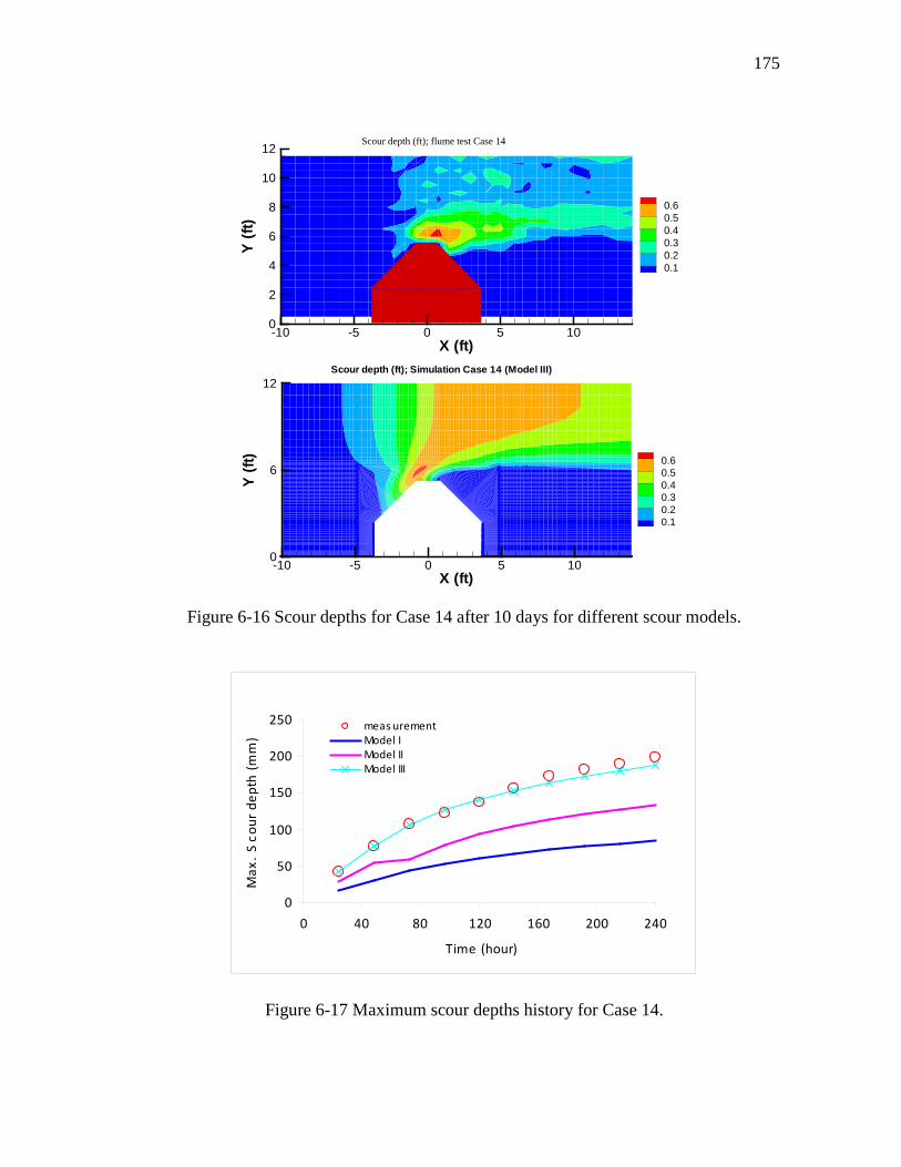
175
X (ft)
Y(ft
)
-10 -5 0 5 100
2
4
6
8
10
12
0.60.50.40.30.20.1
Scour depth (ft); flume test Case 14
X (ft)
Y(ft
)
-10 -5 0 5 100
6
12
0.60.50.40.30.20.1
Scour depth (ft); Simulation Case 14 (Model III)
Figure 6-16 Scour depths for Case 14 after 10 days for different scour models.
0
50
100
150
200
250
0 40 80 120 160 200 240
Time (hour)
Max
. S
cour
dep
th (
mm
)
meas urementModel IModel IIModel III
Figure 6-17 Maximum scour depths history for Case 14.
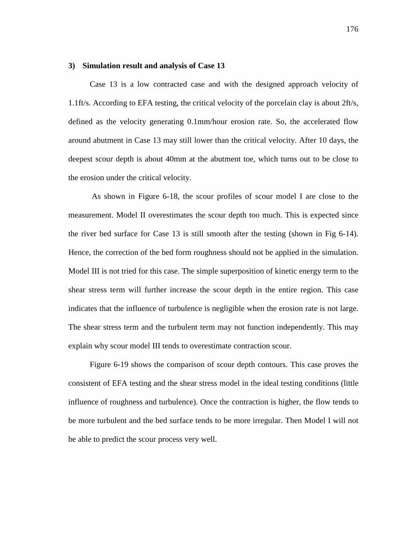
176
3) Simulation result and analysis of Case 13
Case 13 is a low contracted case and with the designed approach velocity of
1.1ft/s. According to EFA testing, the critical velocity of the porcelain clay is about 2ft/s,
defined as the velocity generating 0.1mm/hour erosion rate. So, the accelerated flow
around abutment in Case 13 may still lower than the critical velocity. After 10 days, the
deepest scour depth is about 40mm at the abutment toe, which turns out to be close to
the erosion under the critical velocity.
As shown in Figure 6-18, the scour profiles of scour model I are close to the
measurement. Model II overestimates the scour depth too much. This is expected since
the river bed surface for Case 13 is still smooth after the testing (shown in Fig 6-14).
Hence, the correction of the bed form roughness should not be applied in the simulation.
Model III is not tried for this case. The simple superposition of kinetic energy term to the
shear stress term will further increase the scour depth in the entire region. This case
indicates that the influence of turbulence is negligible when the erosion rate is not large.
The shear stress term and the turbulent term may not function independently. This may
explain why scour model III tends to overestimate contraction scour.
Figure 6-19 shows the comparison of scour depth contours. This case proves the
consistent of EFA testing and the shear stress model in the ideal testing conditions (little
influence of roughness and turbulence). Once the contraction is higher, the flow tends to
be more turbulent and the bed surface tends to be more irregular. Then Model I will not
be able to predict the scour process very well.

177
-4
-3
-2
-1
0
1
0 2 4 6 8 10 12
Scou
r D
epth
(inc
h)
T Station (ft)
Scour Depth Profile at Middle of Abutment
Measurement
Model I
Model II
-4
-3
-2
-1
0
1
0 2 4 6 8 10 12
Scou
r D
epth
(inc
h)
T Station (ft)
Scour Depth Profile at upstream of Abutment
Measurement
Model I
Model II
-4
-3
-2
-1
0
1
0 2 4 6 8 10 12
Scou
r D
epth
(inc
h)
T STation (ft)
Scour Depth Profile at Downstream of Abutment
Measurement
Model I
Model II
Figure 6-18 Scour profiles for Case 13 after 10 days at different cross sections.

178
X (ft)
Y(ft
)
-10 -5 0 5 100
6
12
0.250.20.150.10.05
Scour Depth (ft); Flume test Case13
X (ft)
Y(ft
)
-5 0 5 100
5
10
0.250.20.150.10.05
Scour depth (ft); Simulation Case 13 (Model I)
Figure 6-19 Scour depths pattern for Case 13 after 10 days.
0
20
40
60
80
100
-10 40 90 140 190 240T ime (Hour)
Max
. S
cou
r D
epth
(m
m)
Meas urement
Model I
Model II
Figure 6-20 Maximum scour depths history for Case 13.

179
Figure 6-20 shows the variation of the maximum scour depth at the toe of the
abutment over time. The shear stress model without correction can predict the
measurement very well.
4) Conclusion of the scour simulations on rectangular channel
1. The corrections of roughness and turbulence are required when the contraction
effect of abutment on the rectangular channel is large enough. And scour model III is
still applicable in rectangular channel.
2. Scour model I is applicable to predict the maximum abutment scour depth only
when the bed surface is very smooth and the turbulence is not strong.
6.4 Scour Prediction with Overtopping
Abutment scour under overtopping flow conditions is studied numerically. The
purpose is to get the basic knowledge about the scour development when the flow is
pressurized under the bridge deck. In the numerical study, the bridge is designed with
0.4ft thick deck and 1.2ft clearance. Vertical wall abutment is chosen in the overtopping
flow study. The approach velocity is 1.09 ft/s; the abutment is 3.33ft long; the half width
of the channel is 12ft. For the same designed bridge and above mentioned parameters,
seven cases have been conducted with the upstream water depth varying from 1.2 ft to
2.8 ft. Figure 6-21 shows the cross sections and the velocity magnitude contours of four
representative cases. Case (a) has open channel flow and water surface is almost
touching low chord; Case (b) is the case with water surface just touching low chord.
Case (c) has water surface in flush with deck surface; Case (d) has water surface
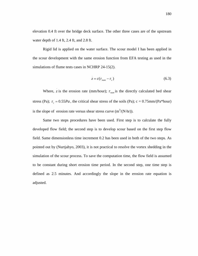
180
elevation 0.4 ft over the bridge deck surface. The other three cases are of the upstream
water depth of 1.4 ft, 2.4 ft, and 2.8 ft.
Rigid lid is applied on the water surface. The scour model I has been applied in
the scour development with the same erosion function from EFA testing as used in the
simulations of flume tests cases in NCHRP 24-15(2).
.
( )num cz c τ τ= − (6.3)
Where, .z is the erosion rate (mm/hour); numτ is the directly calculated bed shear
stress (Pa); 0.55c Paτ = , the critical shear stress of the soils (Pa); c = 0.75mm/(Pa*hour)
is the slope of erosion rate versus shear stress curve (m3/(N·hr)).
Same two steps procedures have been used. First step is to calculate the fully
developed flow field; the second step is to develop scour based on the first step flow
field. Same dimensionless time increment 0.2 has been used in both of the two steps. As
pointed out by (Nurtjahyo, 2003), it is not practical to resolve the vortex shedding in the
simulation of the scour process. To save the computation time, the flow field is assumed
to be constant during short erosion time period. In the second step, one time step is
defined as 2.5 minutes. And accordingly the slope in the erosion rate equation is
adjusted.
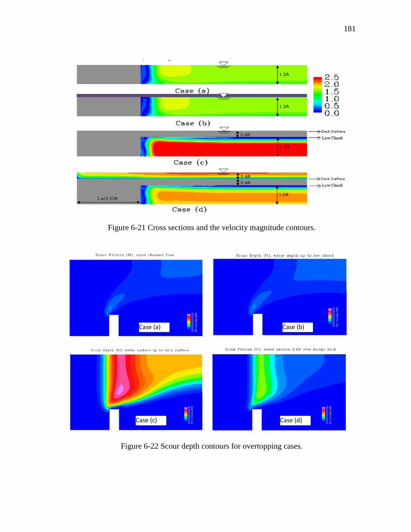
181
Figure 6-21 Cross sections and the velocity magnitude contours.
Figure 6-22 Scour depth contours for overtopping cases.
Case (b) Case (a)
Case (c) Case (d)
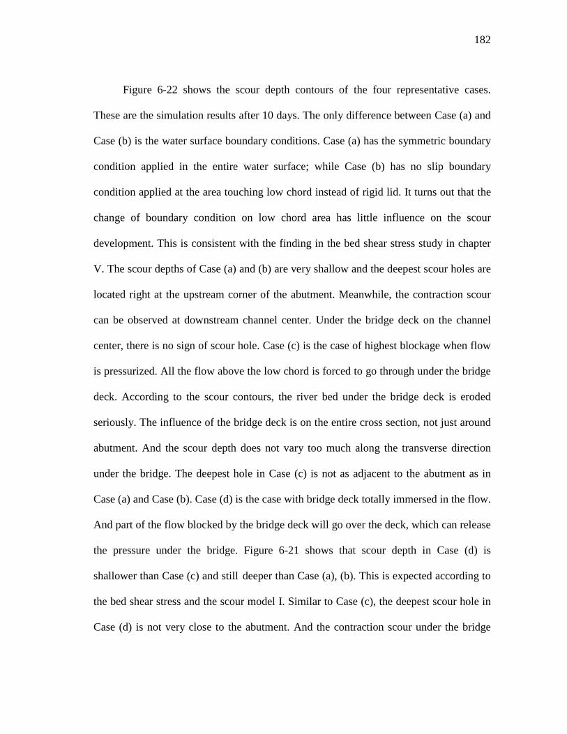
182
Figure 6-22 shows the scour depth contours of the four representative cases.
These are the simulation results after 10 days. The only difference between Case (a) and
Case (b) is the water surface boundary conditions. Case (a) has the symmetric boundary
condition applied in the entire water surface; while Case (b) has no slip boundary
condition applied at the area touching low chord instead of rigid lid. It turns out that the
change of boundary condition on low chord area has little influence on the scour
development. This is consistent with the finding in the bed shear stress study in chapter
V. The scour depths of Case (a) and (b) are very shallow and the deepest scour holes are
located right at the upstream corner of the abutment. Meanwhile, the contraction scour
can be observed at downstream channel center. Under the bridge deck on the channel
center, there is no sign of scour hole. Case (c) is the case of highest blockage when flow
is pressurized. All the flow above the low chord is forced to go through under the bridge
deck. According to the scour contours, the river bed under the bridge deck is eroded
seriously. The influence of the bridge deck is on the entire cross section, not just around
abutment. And the scour depth does not vary too much along the transverse direction
under the bridge. The deepest hole in Case (c) is not as adjacent to the abutment as in
Case (a) and Case (b). Case (d) is the case with bridge deck totally immersed in the flow.
And part of the flow blocked by the bridge deck will go over the deck, which can release
the pressure under the bridge. Figure 6-21 shows that scour depth in Case (d) is
shallower than Case (c) and still deeper than Case (a), (b). This is expected according to
the bed shear stress and the scour model I. Similar to Case (c), the deepest scour hole in
Case (d) is not very close to the abutment. And the contraction scour under the bridge
183
deck is also well developed. However, the affected area at downstream is quite smaller
compared with Case (c). When overtopping, the influence of the bridge deck is also on
the entire cross section.
0.00
0.10
0.20
0.30
0.40
0.50
0.60
0 24 48 72 96 120 144 168 192 216 240
Time (hour)
Max
. Sco
ur d
epth
(ft) d1=0 ft
d1=0.2 ft
d1=0.4 ft
d1=0.8 ft
d1=1.2 ft
d1=1.6 ft
h
d1
y
s=0.4 ft
Figure 6-23 Scour histories of the simulations with overtopping flow.
Figure 6-23 presents the scour histories of the six cases with different water depth.
These six cases can be divided into two groups, pressurized flow and overtopping flow.
If the water surface is between low chord and deck surface, the flow is called pressurized
flow. Actually, the flow with water surface just touching low chord (like Case (b)) is
hardly pressurized. If the water surface is higher than the bridge deck surface, the flow is
called overtopping flow. It should be noted that the flow under the bridge deck is still
pressurized when overtopping occurs. For the three pressurized cases, water surface
elevation varies from low chord to the high chord. The channel contraction ratio
184
increases with the increase of water depth. And the scour depth will also increase. This
can be observed in figure 6-23. For the three overtopping cases, the channel contraction
ratio decreases with the increase of water depth. This explains why the scour depth
decreases with the increase of the water depth when overtopping. Hence, the deepest
scour depth can be reached when water surface is in flush with deck surface. This is the
limiting condition that a flow can generates for a certain bridge. However, the influence
of the water depth on scour development is not large for overtopping conditions when
the water deep enough. This is supported by the difference of the curves of 0.8 ft
overtopping and 1.2 ft of overtopping.
The correction factor of overtopping flow for maximum abutment scour depth
equation will be proposed based on these numerical studies. The influence is evaluated
based on the condition of open channel flow with water surface elevation flush with the
low chord of bridge. Scour is the interaction between flow and soils. All those
parameters affecting shear stress in chapter IV and soil erosion property will impact the
scour development in overtopping situations. The primary actions of flow on soils are
the fluctuating stresses applied on the soil particles. Shear stress component is believed
to be dominant. The maximum bed shear stress is commonly used to represent the
erosion capacity of the flow. The critical shear stress of the soil is used to represent the
erosion resistance of the soil. Hence, the correction is proposed based on the difference
between the maximum bed shear stress and the critical shear stress of soils. However,
the location of the initial maximum bed shear stress may not be same to the final deepest
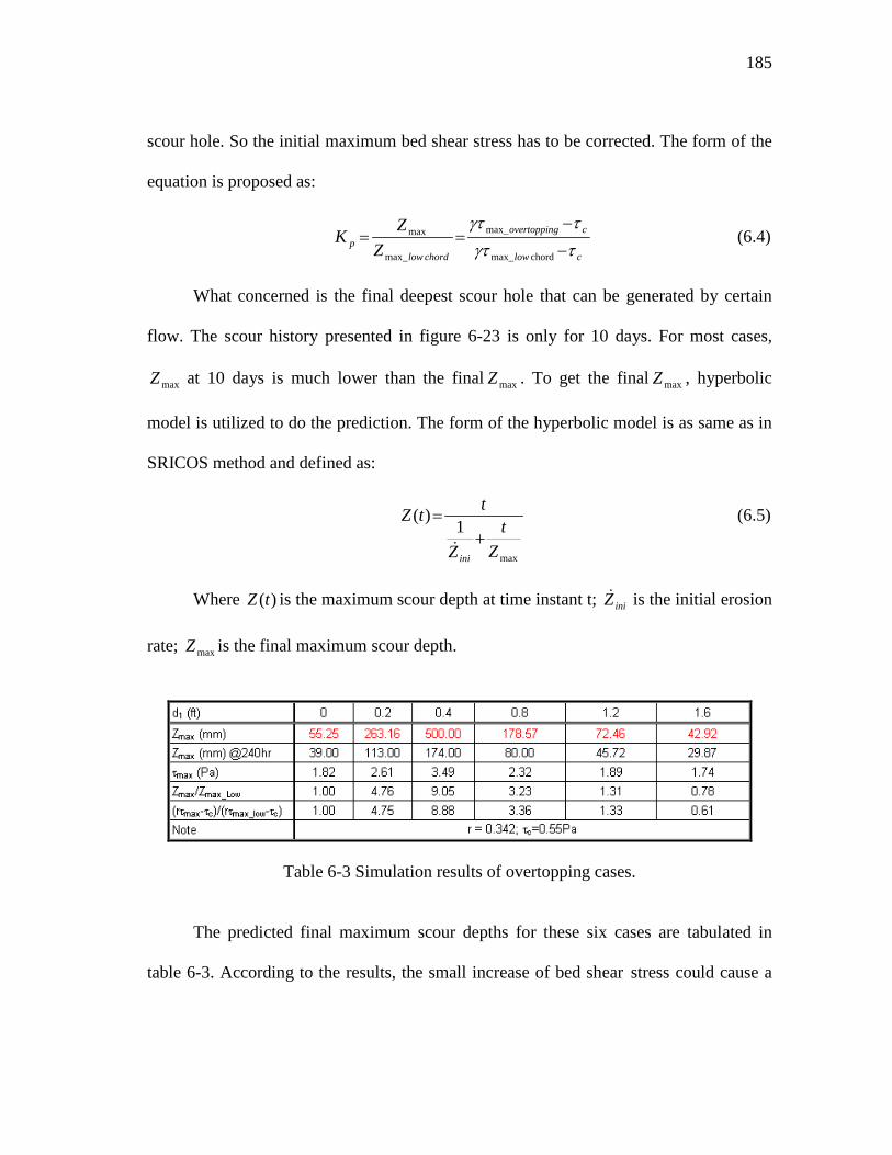
185
scour hole. So the initial maximum bed shear stress has to be corrected. The form of the
equation is proposed as:
clow
cgovertoppin
chordlowp Z
ZK
τγττγτ
−
−==
chord max_
max_
max_
max (6.4)
What concerned is the final deepest scour hole that can be generated by certain
flow. The scour history presented in figure 6-23 is only for 10 days. For most cases,
maxZ at 10 days is much lower than the final maxZ . To get the final maxZ , hyperbolic
model is utilized to do the prediction. The form of the hyperbolic model is as same as in
SRICOS method and defined as:
max
1)(
Zt
Z
ttZ
ini
+=
(6.5)
Where )(tZ is the maximum scour depth at time instant t; iniZ is the initial erosion
rate; maxZ is the final maximum scour depth.
Table 6-3 Simulation results of overtopping cases.
The predicted final maximum scour depths for these six cases are tabulated in
table 6-3. According to the results, the small increase of bed shear stress could cause a
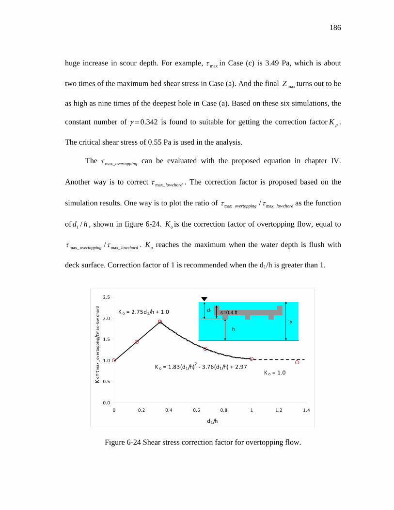
186
huge increase in scour depth. For example, maxτ in Case (c) is 3.49 Pa, which is about
two times of the maximum bed shear stress in Case (a). And the final maxZ turns out to be
as high as nine times of the deepest hole in Case (a). Based on these six simulations, the
constant number of 342.0=γ is found to suitable for getting the correction factor pK .
The critical shear stress of 0.55 Pa is used in the analysis.
The govertoppinmax_τ can be evaluated with the proposed equation in chapter IV.
Another way is to correct lowchordmax_τ . The correction factor is proposed based on the
simulation results. One way is to plot the ratio of max_ max_/overtopping lowchordτ τ as the function
of 1 /d h , shown in figure 6-24. oK is the correction factor of overtopping flow, equal to
max_ max_/overtopping lowchordτ τ . oK reaches the maximum when the water depth is flush with
deck surface. Correction factor of 1 is recommended when the d1/h is greater than 1.
K o = 2.75d1/h + 1.0
K o = 1.83(d1/h)2 - 3.76(d1/h) + 2.97
0.0
0.5
1.0
1.5
2.0
2.5
0 0.2 0.4 0.6 0.8 1 1.2 1.4
d1/h
Ko =τ m
ax_o
vert
oppi
ng/τ
max
-low
cho
rd
K o = 1.0
h
d1
y
s=0.4 ft
Figure 6-24 Shear stress correction factor for overtopping flow.

187
CHAPTER VII
CONCLUSIONS AND RECOMMENDATIONS
7.1 Conclusions
The CHEN3D program has been applied to study the bed shear stress around
abutment in river channel. Based on the systematic parametric studies, the equation has
been proposed to estimate the maximum bed shear stress at the initial conditions of the
scouring. The chimera technique incorporated in the program makes it possible to
simulate the complex channel geometries, such as the channel overtopping, confluence
of the channel. Scour models for clear water scour have been studied. The influence of
bed form roughness and the flow turbulence has been considered in the scour prediction
of the flume tests. The scour under overtopping condition has also been studied
numerically. The followings are the main conclusions obtained in this research:
1. Reynolds number is dominant for the maximum bed shear stress around
abutment. The relationship is not identical to the pier equation because of the
retarding effect of the lateral bank wall and the abutment shape.
2. The shallow water effect is observed in the maximum bed shear stress study
when the relative water depth is small. Froude number is chosen to present the
result.
3. The maximum bed shear stress around abutment is found to be linear
proportional with the channel contraction ratio. The channel contraction ratio

188
should be calculated based on the flow conveyance ratio. The area ratio can be
used only when the upstream flow is uniformly distributed.
4. The maximum bed shear stress decreases with the increase of the aspect ratio of
the approach embankment. When the aspect ratio is large, the influence tends to
be constant.
5. Among the studied abutment shapes, vertical wall abutment can cause the highest
bed shear stress and the spill-through abutment can cause the lowest one. The
shape factor of wing-wall abutment is slightly higher than that for spill-through
abutment.
6. For the abutments with same projected length normal to the flow, the skew angle
of 90 degree can cause the highest bed shear stress. The influence of the skew
angle will decrease when the abutment inclines to either upstream or
downstream.
7. In compound channel, the maximum bed shear stress will increase when the
abutment is very close to the main channel slope.
8. The maximum bed shear stress equation is limited to the hydraulic smooth
boundary. In the actual scouring process, both of the turbulence and the bed
roughness contribute the initial erosion rate. The apparent maximum bed shear
stress has been recommended to compensate the underestimation of the proposed
equation.
9. When channel is overtopping, the maximum bed shear stress around abutment is
found to be the highest when the water surface is in flush with the deck surface.
189
If the water depth continues to increase, the bed shear stress will begin to
decrease.
10. Assuming the blockage effect of the deck is same to the abutment, the proposed
maximum bed shear stress equation is found to be able to predict the maximum
bed shear stress in rectangular channel under overtopping condition with 10% of
difference.
11. Bridge deck tends to make flow more uniform when overtopping occurs. For
rectangular channel, the bed shear stresses increase much faster at channel center
than around abutment. In compound channel, the change of the bed shear stress
at the channel center is not as significant as the rectangular channel because of
the water depth difference between the main channel and the flood plain.
12. For the abutment exists in channel bend suffering open channel flow, the bed
shear stress around the abutment is affected by the channel geometry
significantly when the R/W is small. High curvature can cause the highly non-
symmetric bed shear stress distribution. If the abutment is located in the middle
of the bend, the inner flood plain will have higher bed shear stress. If the
abutment is located at the end of the bend, the outer flood plain will have higher
bed shear stress. The influence of the abutment shape is similar to the straight
channel condition.
13. When overtopping in channel bend, the deck tends to diminish the non-
symmetric feature of flow caused by the bend. The bed shear stress distribution
observed under the deck is basically in symmetry. The abutment location on the
190
bend has little influence to the bed shear stress under the deck. But it will affect
the downstream bed shear stress pattern. If the abutment is in the middle of the
bend, the downstream bed shear stress can recover the non-symmetric pattern.
The influence of the abutment shape still exists under overtopping condition.
14. The tributary upstream can cause the non-symmetric flow and bed shear stress
pattern when the confluence is close to the bridge. The abutment opposite the
tributary may have higher bed shear stress than the other side.
15. Bed shear stress, roughness and flow turbulence all contribute to the scour
development. The contribution of roughness and turbulence may be as same as
the bed shear stress around the abutment. But the turbulence effect is negligible
in the scour development away from the hydraulic structures.
16. The correction factor of the scour under overtopping conditions is found to
depend on both the maximum bed shear stress and critical shear stress of the
soils. The variation of the scour depth with water depth is similar to the trend for
shear stress since the simple shear stress model is applied. But the increase of the
scour depth is much faster than the increase of the bed shear stress when
exceeding the critical shear stress of the bed soils.
7.2 Recommendations
The current research is mainly simulating small scale channels of the flume size
with CHEN3D program (two layer turbulence model). The model scale, the turbulence
model, and the boundary condition might all constrain the universal application of the
major conclusions. The followings are recommended for the future investigations:
191
1. Large eddy simulation should be performed to check the influence of the
turbulence model in the shear stress simulation and the scour prediction.
2. Roughness model should be further developed to reflect the bed roughness effect,
especially the bed form roughness.
3. Based on the flume tests, the velocity fluctuation is found to be related with the
scour development at the downstream side of abutment. The study of the scour
model in clear water scour can be performed toward that direction.

192
REFERENCES
Abed, L. M. 1991 Local scour around bridge piers in pressure flow. Ph.D. Dissertation,
C.E. Dept., Colorado State Univ., Fort Collins, CO.
ABSCOUR USERS MANUAL 2007 Maryland State Highway Administration, Baltimore,
MD.
Arneson, L.A. 1997 The effects of pressure flow on local scour in bridge openings.
Ph.D. Disseration, C.E. Dept., Colorado State Univ., Fort Collins, CO.
Arulanandan, K. 1975 Fundamental aspects of erosion in cohesive soils. J. of Hydraulic
Division, ASCE, 101, 635-639.
Arulanandan, K., Loganathan, P. & Krone, R.B. 1975 Pore and eroding fluid influences
on surface erosion of soil. J. of Geotechnical Engineering, 101, 51-66.
Awazu, S. 1967 On scour around spur dikes. In Proc. of 12th Congr. of the Intl. Assn. for
Hydraulic Research, 3, C12, Delft, The Netherlands.
Briaud, J.-L., Ting, F., Chen, H.C., Gudavalli, S.R., Kwak, K., Philogene B., Han S.-W,
Perugu, S., Wei, G., Nurtjahyo, P., Cao Y.W. & Li, Y. 1999 SRICOS: prediction of
scour rate in cohesive soils at bridge piers, TTI Report No. 2937-1, Department of
Civil Engineering, Texas A&M University, College Station, Texas.
Briaud, J.-L., Ting, F., Chen, H.C., Cao, Y., Han, S.-W., Kwak, K. 2001 Erosion
function apparatus for scour rate predictions. J. of Geotechnical and
Geoenvironmental Engineering, ASCE, 127, 105-113
193
Briaud J.-L., Chen H.-C., Li Y., Nurtjahyo P., Wang J. 2003 Complex pier scour and
contraction scour in cohesive soils, NCHRP Report 24-15, Transportation Research
Board, National Research Council, Washington, DC.
Cao, Y. 2001 The influence of certain factors on the erosion functions of cohesive soil.
M.S. Thesis, Texas A&M University, College Station, TX.
Cebeci, T. & Bradshaw, P. 1977 Momentum transfer in boundary layers. Hemisphere
Publishing Corporation, Washington, DC.
Chabert, J., & Chauvin, J.L. 1963 Formation de dunes et de rides dans les modeles
fluviaux. Bull. Cen. Rech. Ess. Chatou, 4, 345-376.
Chen, C.J & Chen, H.C. 1982 The finite analytic method. IIHR Report No. 232-IV, Iowa
Institute of Hydraulic Research, University of Iowa, Iowa City.
Chen, C.J & Chen, H.C. 1984 Finite analytic numerical method for unsteady two-
dimensional Navier-Stokes equation. J. of Computational Physics, 53, 210-226.
Chen, H.C. & Patel, V.C. 1988 Near-wall turbulence models for complex flows
including separation. AIAA Journal, 26, 641-648.
Chen, H.C. & Patel, V.C. 1989 The flow around wing-body junctions. In Proc. 4th
Symposium on Numerical and Physical Aspects of Aerodynamic Flows, 1-15, Long
Beach, CA.
Chen, H.C., Patel, V.C., & Ju, S. 1990 Solutions of Reynolds-averaged Navier-Stokes
equations for three-dimensional incompressible flows. J. of Computational Physics,
88, 305-336.
194
Chen, H.C. & Korpus, R.A. 1993 A multi-block finite-analytic Reynolds-averaged
Navier-Stokes method for 3D incompressible flow. Individual Papers in Fluids
Engineering, ASME, 150, 113-121.
Chen, H.C. 2002 Numerical simulation of scour around complex piers in cohesive soil.
In Proc. of First International Conference on Scour of Foundation, 14-33, Texas
A&M University, College Station.
Dufresne, M., Vazquez, J., Terfous, A., Ghenaim, A., Poulet, J.-B. 2007 Prediction of
sedimentation in a storm-water tank pilot using computational fluid dynamics. Ninth
International Symposium on Fluid Control, Measurement and Visualization, ID 27
Tallahassee, FL.
Dunn, I. S. 1959 Tractive resistance of cohesive channels. J. of Soil Mechanics and
Foundation Division, ASCE, 85, 1-24.
Durbin, P.A., Medic, G., Seo, J.M., Eaton, J.K. and Song, S. 2001 Rough wall
modification of two-layer ε−k . J. of Fluids Engineering. 123, 16-21.
Hjorth, P. 1975 Studies on nature of local scour. Bulletin Series A. No. 46, Department
of Water Resources Engineering, Lund Institute of Technology/University of Lund,
Sweden.
Ivarson, W.R. 1998 Scour and erosion in clay soils. ASCE Compendium of Conference
Scour Papers (1991 to 1998), 104-119.
Jiang, J., Ganju, N.K. & Menta, A.J. 2004 Estimation of contraction scour in riverbed
using SERF. J. of Waterway, Port, Coastal, and Ocean Engineering, 130, 215-218
195
Jones, J.S., Bertoldi, David, A. & Umbrell, E.R. 1993 Preliminary studies of pressure
flow scour, In Proceedings of the ASCE Hydraulic Engineering Conference, San
Francisco, CA.
Knight, D.W. & Demetriou, J.D. 1983 Flood plain and main channel flow interaction. J.
of Hydraulic Engineering, 109, 1073-1092.
Li, Y. 2002 Bridge pier scour and contraction scour in cohesive soils on the basis of
flume test. Ph.D. Dissertation, Department of Civil Engineering, Texas A&M
University, College Station.
Liu, H.K. 1957 Mechanics of sediment-ripple formation. J. Hyd. Div. ASCE, 183 (HY2),
1-23
Liu, T.J. 2002 Time-domain simulation of large-amplitude ship motions including
capsizing. Ph.D. Dissertation, Department of Civil Engineering, Texas A&M
University, College Station.
Melville, B. W. 1997 Pier and abutment scour: integrated approach. J. of Hydraulic
Engineering, ASCE, 123, 125-136.
Mirtskhoulava, 1988 Basic physics and mechanics of channel erosion. Gidometeoizdat,
Leningrad.
Molinas, A., Kheireldin, K. & Wu, B. 1998 Shear stress around vertical wall abutments.
J. of Hydraulic Engineering, 124, 822-830
Munson, B.R., Young, D.F. & Okiishi, T.H. 1998 Fundamentals of fluid mechanics,
Wiley, New York

196
Myers, W.R.C. & Brennan, E.K. 1990 Flow resistance in compound channels. J. of
Hydraulic Research, 28 (2), 141-155
Naot, D., Nezu, I. & Nakagawa, H. 1993 Hydrodynamic behavior of compound
rectangular open channels. J. of Hydraulic Engineering, 119, 390-408
Nurtjahyo, P. 2003 Chimera RNAS simulations of pier scour and contraction scour in
cohesive soils. Ph.D. Dissertation, Texas A&M University, College Station.
Oh, S.J., 2008 Experimental study of bridge scour in cohesive soils. Ph.D. Dissertation,
Department of Civil Engineering, Texas A&M University, College Station.
Parchure, T.M. & Mehta, A.J. 1985 Erosion of soft cohesive sediment eeposit. J. of
Hydraulic Division, ASCE, 111, 1309-1326
Patel, V.C. & Yoon, J.Y. 1995 Application of turbulence models to separated flow over
rough surfaces. J. of Fluid Engineering, 117, 234-241.
Rajaratnam, N. & Ahmadi, M. 1979 Interaction between main channel and flood-plain
flows. J. of Hydraulic Division, 105 (HY5), 573-588.
Rajaratnam, N. & Nwachukwu, B. 1983 Flow near groin-like structure. J. of Hydraulic
Engineering, 109, 463-480.
Richardson, E. V. & Davis, S. M. 2001 Evaluating scour at bridges, FWHA-IP-90-017,
HEC No.18, US Department of Transportation, Washington, D. C.
Shaikh, A., Ruff, J. F., & Abt, S. R. 1988 Erosion rate of compacted Na-Montmorillonite
soils. J. of Geotechnical Engineering, ASCE, 114, 296–305.
197
Shirole, A.M., and Holt, R.C. (1991), “Planning for comprehensive bridge safety
assurance program.” Transp. Res. Rec. 1290, Transportation Research Board,
Washington, D.C., 137-142.
Simons, D.B.& Richardson, E.V. 1963 Form of bed roughness in alluvial channels.
Trans. ASCE, 128, 284-323
Simons, D.B.& Richardson, E.V. 1966 Resistance to flow in alluvial channels.
Professional Paper 422-J. Washington, D.C., U.S. Geological Survey,
Smerdon, D.B. & Beasley, M.L. 1959 Tractive force theory applied to stability of opens
channels in cohesive soils. Research Bulletin No. 715, Agricultural Experiment
Station, The University of Missouri, Columbia.
Suhs, N. E. & Tramel, R. W. 1991 PEGSUS 4.0 Users Manual. Arnold Engineering
Development Center Report, AEDC-TR-91-8, Arnold Air Force Station, TN.
Tingsanchali, T. & Maheswaran, S. 1990 2-D Depth averaged flow computation near
groyne. J. of Hydraulic Engineering, 116, 71-86.
Umbrell, E.R., Kenneth, Y.G., Stein, S.M. & Jones, J.S. 1998 Clearwater contraction
scour under bridges in pressure flow. J. of Hydraulic Engineering, ASCE, 124, 236-
240
van Rijn, L. C. 1984a Sediment transport: Part I: bed load transport J. of Hydraulic
Engineering, 110, 1431-1456.
van Rijn, L. C. 1984b Sediment transport: Part II: suspended load transport. J. of
Hydraulic Engineering, 110, 1613-1641.

198
van Rijn, L. C. 1984c Sediment transport: Part III: bed form and alluvial roughness. J. of
Hydraulic Engineering, 110, 1733-1754.
Wei, G., Chen, H.C., Ting, F, Briaud, J.-L, Gudavalli, S.R. & Perugu, S. 1997 Numerical
simulation to study scour rate in cohesive soils. Research Report prepared for the
Texas Department of Transportation, Department of Civil Engineering, Texas A&M
University, College Station.
Winterwerp, J.C. 1989 Cohesive sediments, flow included erosion of cohesive beds.
Rijkswaterstaat / Delft Hydraulics, Delft.
Wolfstein, M. 1969 The velocity and temperature distribution in one-dimensional flow
with turbulence augmentation and pressure gradient. Intl. J. of Heat and Mass
Transfer, 12, 301-318.
Wormleaton, P.R. & Merrett, D.J. 1990 An improved method of calculation for steady
uniform flow in prismatic main channel/flood plain sections. J. of Hydraulic
Research, 28, 157-174
Yalin, M.S. 1964. Geometrical properties of sand waves. J. Hyd. Div. ASCE, 90 (HY5),
105-119.
Zaghloul, N.A. 1974 Analytical and experimental investigation of flow around spur
dikes. Ph.D. Dissertation, Department of Civil Engineering, University of Windsor,
Ontario, Canada.
Zhang, H., Faghri, M. & White, F.M. 1996 A New low-Reynolds-number ε−k model
for turbulent flow over smooth and rough surfaces. J. of Fluids Engineering, 118,
255-259.
199
VITA
Xingnian Chen was born in Liaoning, China. He earned his Bachelor of
Engineering in Civil Engineering in July 1997 and sequentially the Master of
Engineering in Geotechnical Engineering in June 2000 from Tongji University, China.
From March 2000 to July 2003, he was a researcher with Shanghai Seakon Engineering
Research and Consulting Center, China. In August 2003, he entered Texas A&M
University, where he served as a research assistant with the Texas Transportation
Institute. He completed his Ph.D. in Civil Engineering in December 2008. His research
was on numerical study of abutment scour. His research interests are fluid-structure-soil
interaction, and soil improvement.
Permanent Address
Xingnian Chen
c/o: Dr. Jean-Louis Briaud
Zachry Department of Civil Engineering
Texas A&M University
College Station, TX, 77840-3136