THE NUMERICAL STUDY OF THE FLOW AND

HEAT TRANSFER BETWEEN TWO HORIZONTAL

CYLINDERS

HUO YUNLONG (B. Eng.)

DEPARTMENT OF MECHANICAL ENGINEERING

A THESIS SUBMITTED

FOR THE DEGREE OF MASTER OF ENGINEERING

NATIONAL UNIVERSITY OF SINGAPORE

2004

I

ACKNOWLEDGEMENT

The author wishes to record here his indebtedness and gratitude to many who

have contributed their time, knowledge and effort towards the fulfillment of this work.

Particularly, he would like to express his heartfelt gratitude and thanks to Dr. T. S. Lee

and Dr H. T. Low for their invaluable guidance, supervision, encouragement and

patience throughout the course of the investigation.

The technical staffs of the Fluid Mechanics Laboratory are also to be thanked

for their assistance during the phase of the investigation. Special thanks are also due to

my classmates in the Fluid Mechanics Laboratory who give me great help in plotting

the figures and using the Tecplots.

The author also wants to express his appreciation to his last grandfather whose

spirit encourages him, supports him and assists him throughout this period.

Finally, the author wished to express his gratitude to those who have directly or

indirectly contributed to this investigation.

II

SUMMERY

The flow and convective heat transfer in concentric and eccentric horizontal

annuli with isothermal wall conditions are studied numerically using two-dimensional

finite-difference and finite-element models. The Stream-Function Vorticity and

primitive variable formulations are applied to the finite different and finite element

methods respectively. The structure mesh is obtained to simulate the buoyancy driven

flow. Since the complex geometry configuration of the studied cases, the cylindrical

and bipolar coordinates are introduced to solve problems of the finite difference

method. The model is also designed by the Galerkin finite element method with Penalty

Function Approach. The effects of various parameters such as the radius ratio of the

annulus, the eccentricity of the annulus, the Rayleigh number and Reynolds number of

the rotation of the inner cylinder are investigated at the Prandtl number of 0.701.

Overall heat transfer results are obtained. For the case of concentric cylinders, the

numerical results obtained are in good agreement with the similar results of other

investigators. In the extension of the numerical work done here, rotating the inner

cylinder and outer cylinder individually and both are also considered. For the eccentric

cases, comparison with available experimental results with the present two-dimensional

numerical model is good at relatively low Reynolds numbers in the range of 0-800. The

effects of Prandtl number on the flow and heat transfer are also briefly studied in the

present investigations. All of the kidney cells, the stagnant zone and the thermal plume

are changed with different directions and velocities of the rotation, Rayleigh number,

eccentric ratio and Prandtl number.

III

TABLE OF CONTENTS

Page

ACKNOWLEDGEMENT I

ABSTRACT II

NOMENCLATURE V

LIST OF FIGURES VIII

CHAPTER 1 INTRODUCTION

1.1 Background 1

1.2 Literature survey 2

1.3 Flow description 9

1.4 Objectives and scope 12

CHAPTER 2 PROBLEM FORMULATION

2.1 Derivations of the governing equations 14

2.2 Coordinate system for finite difference method 18

2.3 The governing equation and boundary condition in finite element method 19

2.4 Investigated geometric and physical parameters 22

2.5 Boundary conditions in the finite difference method 24

CHAPTER 3 NUMERICAL METHODS

3.1 The finite-difference and finite-element approaches 27

3.2 The solution procedure 28

3.3 Finite difference methods for solving the equations 30 3.4 Finite element methods for solving the equations 37

IV

CHAPTER 4 ANALYSIS OF RESULTS FOR THE FINITE ELEMENT

METHOD

4.1 The effect of Rayleigh numbers 41

4.2 The effect of the radius ratio 42

4.3 The effect of eccentricity 43

4.4 The effect of rotating the inner and/or outer cylinders between concentric cases 45

4.5 The effect of rotating the inner and/or outer cylinders between eccentric

cylinders 47

CHAPTER 5 ANALYSIS OF RESULTS FOR THE FINITE DIFFERENCE

METHOD

5.1 The effects of Rayleigh numbers 51

5.2 The effects of radius ratio 52

5.3 The effect of the inner cylinder rotating 53

5.4 The effects of eccentricity 55

5.5 The effects of rotating inner cylinder in the eccentric annulus 57

CHAPTER 6 CONCLUSIONS AND RECOMMENDATIONS 60

REFERENCES 62

FIGURES 68

V

NOMENCLATURE

A Area

C Constant in the transformation equations from Bipolar coordinate systems to

Cartesian Coordinate System

D Diameter

E Magnitude of the eccentricity vector, −e , e = |

−e |

−e Eccentricity Vector,

−e = ( vh ee , )

re Magnitude of the eccentricity ratio vector r

e−

, re = | r

e−

|

re−

Eccentricity ratio vector, r

e−

=−e /L

g Gravity acceleration, g=| −g |

−g Gravity vector

ηξ hh , Metric or scale factors in the Bipolar coordinate system

gi Unit vector in the direction of the gravity vector, gi =−g /g

k Thermal conductivity

eeqk Overall equivalent thermal conductivity

eqlk Local equivalent thermal conductivity

L ‘mean’ clearance between the two cylinders, L= io rr −

DNu Nusselt number based on the diameter of the heated cylinder, kDhNuD /−

=

p, P Pressure

Pr Prandtl number, Pr = αυ /

r radius

VI

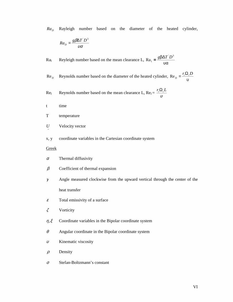
DRa Rayleigh number based on the diameter of the heated cylinder,

υαβ 3'DTgRaD∆=

Ral Reyleigh number based on the mean clearance L, υα∆β 3DTg '

====lRa

DRe Reynolds number based on the diameter of the heated cylinder, υ

Ω=

Dr iiDRe

Rel Reynolds number based on the mean clearance L, Rel = υ

Lr iiΩ

t time

T temperature

−U Velocity vector

x, y coordinate variables in the Cartesian coordinate system

Greek

α Thermal diffusivity

β Coefficient of thermal expansion

γ Angle measured clockwise from the upward vertical through the center of the

heat transfer

ε Total emissivity of a surface

ζ Vorticity

ξη , Coordinate variables in the Bipolar coordinate system

θ Angular coordinate in the Bipolar coordinate system

υ Kinematic viscosity

ρ Density

σ Stefan-Boltzmann’s constant

VII

φ Angular position of the gravity vector relative to the negative y-axis measured

in the clockwise direction

ψ Stream function

Ω Angular speed

Subscripts

i stands for inner cylinder; also used as an indexing integer variable for the mesh

points

o stands for outer cylinder

r stands for reference quantity; also used as an indexing integer variable for the

mesh points

w stands for wall

Superscripts

k number of the inner iteration

n number of the time step or global iteration

‘ the ‘prime’ symbol emphasizes the dimensional form of a variable as distinct from its

non-dimensional usage

VIII

LIST OF FIGURES

Table 3.1 Shape Functions of Quadrilateral Elements (4-9) 70 Table 4.1 Parameters used in calculations 70 Fig. 1.1.1 Geometry of annular region and the gravity direction 68 Fig. 2.1.1 Mesh used for the numerical computation 68 Fig. 3.1.1 2-D view of three kinds of shape function 69

Fig. 4.1.1 – 4.5.5 Figures for finite element method Fig. 4.1.1 – 4.1.5 Flow and temperature fields for various Rayleigh numbers of air (71-73) Fig. 4.2.1 – 4.2.2 Flow and temperature fields for various Radius ratio of air (74-75) Fig. 4.3.1 – 4.3.4 Flow and temperature fields for various eccentric ratio of air (76-78) Fig. 4.4.1 – 4.4.4 Flow and temperature fields for various rotations in concentric

annulus (79-82) Fig. 4.5.5 – 4.5.5 Flow and temperature fields for various rotations in eccentric

annulus (83-87)

Fig. 5.0.1 – 5.5.6 Figures for finite difference method Fig. 5.0.1 Overall heat transfer coefficient versus Rayleigh number at the

radius ratio of 2.6, 0=re . (88-88) Fig. 5.1.1 – 5.1.2 Flow and temperature fields for various Rayleigh numbers of air (89-90) Fig. 5.2.1 – 5.2.3 Flow and temperature fields for various Radius ratio of air (91-93) Fig. 5.3.1 – 5.3.2 Flow and temperature fields for various rotations in concentric

annulus (94-95) Fig. 5.4.1 – 5.4.3 Flow and temperature fields for various eccentric ratio of air (96-98) Fig. 5.5.1 – 5.5.6 Flow and temperature fields for various rotations in eccentric

annulus (99-104)

1

CHAPTER 1 INTRODUCTION

1.1 Background

The flow and thermal fields in enclosed space have received much attention

because of theoretical and wide engineering applications, such as thermal energy

storage systems, cooling of electronic components, and transmission cables. Fig. 1.1.1

shows the Geometry of annular region and the gravity direction. Given the problem

illustrated in Fig. 1.1.1, the inner circular is set to high temperature and the outer part

lower temperature under the terrestrial conditions. Due to its simple geometry and well-

defined boundary conditions, the system has been studied extensively by researchers

such as Bishop et al (1968), Kuehn and Goldstein (1976), Farouk and Guceri (1981),

Vafai and Desai (1993), and large number of literatures were published in the past few

decades. For concentric and eccentric cases in a horizontal annulus between two

circular cylinders, the basic and fundamental configuration, the flow and thermal fields

have been well studied. Kuehn and Goldstein (1976) comprehensively studied the

concentric case. The experimental and numerical studies of the eccentric case have also

been conducted by Kuehn and Goldstein (1978), and Guj and Stella (1995). However,

on the whole, little is known about effects of rotation of inner and/or outer cylinders on

the flow and the heat transfer in eccentric annuli. There is much scope for further

investigation in this aspect of the problem. The numerical method of both of finite

element and finite partial difference methods are useful. In present work the author

focuses on two parts. In the first part, based on the previous work, the primary aim is to

extend knowledge into areas that have not been conducted and examined. The main

methods are the finite element method and the finite difference approach. For the finite

element method, original governing equations are used to produce the velocity field and

2

temperature distribution. For the finite difference method, the streamline plot is created

through using Stream-Function Vorticity formulation. Compared with each other, both

of the two methods are capable of solving the flow and the convective heat transfer in

concentric and eccentric horizontal annuli with isothermal wall conditions. Compared

with the results of Kuehn and Goldstein (1976), the computed results of the thesis also

show that the study may be pushed further to enter the second part. The second part is

the knowledge extension that has a little study by other investigators. The primary

objectives of this part focus on natural convection in the eccentric horizontal annuli

where both inner and outer cylinders are rotated. Both rotated inner and outer cylinders

are seldom investigated by other researchers. Different kinds of rotation such as the

same direction of the inner and outer cylinders, and the opposite direction of the inner

and outer cylinders associated with the eccentric ratio will be discussed in the thesis.

Particularly, when the Reynolds number is large, the unstable situation is produced.

1.2 Literature review

Natural convection between horizontal concentric cylinders has been widely

studied experimentally and numerically over the past three decades because of the

importance of this subject in industries, such as transmission cable cooling systems,

latent energy storage systems, nuclear reactor designs, etc. The problem was first

investigated experimentally by Beckmann (1931) with air, hydrogen and carbon

dioxide as the test fluids to obtain overall heat transfer coefficients. A large part of the

experimental work was devoted to finding the overall heat transfer between the

cylinders using the non-dimensional parameter defining the temperature difference

between the cylinders. Particularly Kuehn and Goldstein (1976) investigated the

problem experimentally and numerically. A Mach-Zehnder interferometer was used to

3

determine the temperature distribution and the local heat transfer coefficients in air and

water. With water, they demonstrated that the flow remained steady even though the

Rayleigh number was well over the critical value obtained experimentally with air,

which suggests that the Prandtl number affected the transition characteristics.

Unlike the case of natural convection in concentric annulus, similar

experimental studies for eccentric annulus are few. The effect of vertical and horizontal

eccentricities on the overall heat transfer coefficient was first experimentally

investigated by Zagromov and Lyalikov (1966) using air as the working fluid. Using

optical interferometry, Kuehn and Goldstein (1978) studied the local and overall heat

transfer coefficients for both horizontal and vertical eccentricities of magnitude re up

to about 2/3. They found that although the distribution of the local heat transfer

coefficient was substantially altered by eccentricity, the overall heat transfer coefficient

did not change by more than 10% from the concentric value at the same Rayleigh

number. The effect of moving the inner cylinder downwards is to cause the overall heat

transfer to increase while moving the inner cylinder upwards has the opposite effect.

Yeo (1984) use the same method as Kuehn and Goldstein (1976, 1978) to verify the

overall heat transfer coefficients predicted by the numerical model. His experimental

results are in good agreement with the experimental results of Kuehn and Goldstein

(1978) obtained using nitrogen as test fluid and fit the present numerical curve very

well with deviations typically less than 5%. Lee (1991) performed the numerical

experiments to study rotational effects on the mixed convection of low-Prandtl-number

fluids enclosed between the annuli of concentric and eccentric horizontal cylinders. For

the range of Prandtl numbers considered here, numerical experiments showed the mean

Nusselt number increases with increasing Rayleigh number for both concentric and

eccentric stationary inner cylinders. At a Prandtl number of order 1.0 with a fixed

4

Rayleigh number, when the inner cylinder is rotated, the mean Nusselt number

decreases throughout the flow. Dennis and Sayavur (1998) analytically and

experimentally investigated the flow in eccentric annuli of drilling fluids commonly

used in oil industry. The expression for azimuthal velocity as a function of eccentricity

ratio and rheological parameters of the fluid has been obtained based on the linear

fluidity model. Velocity profiles were measured for a Newtonian glycerol/water

mixture and a non-Newtonian oil field spacer fluid in eccentric annuli using the

stroboscoptic flow visualization method.

Because of the limitations of the analytical approach and encouraged by the

availability of large computing machines, numerical methods were applied to solve the

equations which govern the flow and heat transfer in the annulus.

The first numerical solution was obtained by Crawford and Lemlich (1962)

using a Gauss-Seidel iterative method. Abbot (1962) used a matrix inversion technique

to obtain solutions for the case of narrow annuli. Powe et al. (1971) applied numerical

method to determine the Rayleigh number for the onset instability in the flow at

relatively low radius ratios and obtained reasonably good qualitative agreement with

the earlier experimental results of Powe et al. (1969) on the delineation of the flow

regimes. Their numerical results seem to indicate that the onset of multicellular flow at

low radius ratios does not affect the overall heat transfer significantly. Charrier-Mojtabi

et al. (1980) gave numerical solutions using the alternating direction implicit (ADI)

method for three cases: a wide annulus (R=2.26) for Pr=0.7, a narrow annulus (R=1.2)

for Pr=0.7 and a wide annulus (R=2.5) for Pr=0.02. On treating the problem

numerically at high Rayleigh numbers, Jischke and Farshch (1980) divided the flow

field of an annulus into five regions which include an inner boundary layer near the

inner cylinder, an outer boundary layer near the outer cylinder, a vertical plume region

5

above the inner cylinder, a stagnant region below the inner cylinder and a core region

surrounded by these four regions; they applied the boundary layer approximation to

obtain the temperature distribution and heat transfer rates. A numerical parametric

study was carried out by Kuehn and Goldstein (1980), in which the effects of the

Prandtl number and the radius ratio on heat transfer coefficient were investigated.

Tsui and Tremblay (1984) presented the results of mean Nusselt numbers for

both transient and the steady natural convection. San Andres (1984) found the size of

the separation eddy and the position of the points of separation and reattachment to be

Reynolds number dependent in the numerical study of flow between eccentric

cylinders. The separation point moves in the direction of rotation upon increasing the

Reynolds number, in contradiction of the first-order inertial perturbation theory of

Ballal and Rivlin (1976). The numerical methods employed in their study include

Galerkin’s procedure with B-spline test function. Galpin and Raithby (1986) assessed

the impact of the ‘standard’ treatment of the T-V coupling and proposed an improved

method. Newton-Raphson linearization was investigated as a means of accelerating the

convergence rate of control volume-based predictions of natural convection flow. It is

found that repeated solutions of the Newton-Raphson linear set converge monotonically

for a much wider range of relaxation, and the maximum convergence rate can be

significantly higher than that corresponding to the standard linear set.

Lee and Yeo (1985) developed a numerical model to study the effects of

rotation on the fluid motion and heat-transfer processes in the annular space between

eccentric cylinders when the inner cylinder is heated and rotating. The overall

equivalent thermal conductivity ( eqK ) is obtained for Rayleigh numbers Ra up to 610

with rotational Reynolds number Re variations of 0-1120. Investigation shows that, for

Re up to the order of 102, the numerical model shows promising results when Ra is

6

increased. Numerical solutions for laminar, fully developed, forced convective heat

transfer in eccentric annuli were presented by Manglik and Fang (1995). With an

insulated outer surface, two types of thermal boundary conditions had been considered:

constant wall temperature (T), and uniform axial heat flux with constant peripheral

temperature (H1) on the inner surface of the annulus. Velocity and temperature profiles,

and isothermal Re, Nui,j and Nui,H values for different eccentric annuli ( 6.00 * ≤≤ ε )

with varying aspect ratios ( 75.025.0 * ≤≤ r ) are presented in their paper. The

eccentricity is found to have strong influence on the flow and temperature fields. The

flow trends to stagnate in the narrow section and has higher peak velocities in the wide

section. The flow maldistribution is found to produce greater nonuniformity in the

temperature field and degradation in the average heat transfer. Yoo (1998) numerically

investigated dual steady solution in natural convection in an annulus between two

horizontal concentric cylinders for a fluid of Prandtl number 0.7. It is found that when

the Rayleigh number based on the gap width exceeds a certain critical value, dual

steady two-dimensional (2-D) flows can be realized: one being the crescent-shaped

eddy flow commonly observed and the other the flow consisting of two counter-

rotating eddies and their mirror images. The critical Rayleigh number decreases as the

inverse relative gap width increases.

Mohamed etc. (1998) numerically studied the effect of radiation on unsteady

natural convection in a two-dimensional participating medium between two horizontal

concentric and vertically eccentric cylinders by using a bicylindrical coordinates

system, the stream function, and vorticity. Original results are obtained for three

eccentricities, Rayleigh number equal to 104, 105 and a wide range of radiation-

conduction parameter. Shu and Yeo (2000) applied the global method of polynomial-

based differential quadrature (PDQ) and Fourier expansion-based differential

7

quadrature (FDQ) to simulate the natural convection in an annulus between two

arbitrarily eccentric cylinders. Their approach combined the high efficiency and

accuracy of the differential quadrature (DQ) method with simple implementation of

pressure single value condition. The result confirmed the finding by Guj and Stella

(1995). Escudier et al. (2000) concerned a computational and experimental study of

fully developed laminar flow of a Newtonian liquid through an eccentric annulus with

combined bulk axial flow and inner cylinder rotation. Their results were reported for

calculation of the flow field, wall shear stress distribution and friction factor for a range

of values of eccentricity ε , radius ratio κ and Taylor number Ta. More recently, Lee et

al. (2002) used GDQ method due to the eccentricity of the inner and outer cylinders

studied the nett fluid circulation around the inner cylinder and the effects of rotation of

the inner cylinder with a radius ratio of 2.6.

Discrepancies among the results reported in the literature for narrow annuli are

found by Rao et al. (1985), Fant et al. (1989), Cheddadi et al. (1992), Kim and Ro.

(1994). Large differences are shown not only for the Ra values at which bifurcation

occur but also in regard to a possible existence of hysteresis phenomena. For example,

Kim and Ro (1994) and Fant et al. (1989) found a hysteresis numerically, whereas Rao

et al. (1985) show only one type of multicellular flow. Cheddadi et al. (1992) presented

two numerical solutions at the same Ra that depends on the initial conditions: the

crescent base flow and a multicellular one. However, they failed to obtain multicellular

flows experimentally. Rao et al. (1985) and Kim and Ro (1994) supported numerically

the general trends presented by Powe et al. (1969); that is, the appearance of

multicellular flow patterns in the upper part of narrow annuli. Furthermore, Rao et al.

(1985) reported a transition of the steady upper cells to oscillatory motion at moderate

Rayleigh numbers. Using a linear stability analysis of steady two-dimensional natural

8

convection of a fluid layer confined between differentially heated vertical plane walls,

Korpela et al. (1973) reported that the flow is primarily unstable against purely

hydrodynamic steady waves in the limit of zero Prandtl number. These secondary

shear-driven instabilities are crossing cells called “cat’s eyes.” Increases in Prandtl

number lead to the appearance of buoyancy-driven oscillatory instabilities. The critical

value of Pr determining which type of instabilities appears has been numerically

determined which type of instabilities appears has been numerically determined to be

around Pr=12.7 by many authors. In slots of finite ratio of height over width the vertical

temperature gradient is an additional results and linear stability analysis, Roux et al.

(1980) have demonstrated the existence of a zone of limited extent in the (Ra, A)-plane

inside which steady cat’s eyes can develop. This zone is only for aspect ratios larger

than about A=11 for air-filled cavities. This result was confirmed by the numerical

studies of Lauriat (1980), Lauriat and Desrayaud (1985), and more recently by Le

Quere (1990) and Wakitani (1997). As Ra is further increased, a reverse transition from

multicellular flow to unicellular flow occurs and this has been numerically and

experimentally demonstrated by Roux et al. (1980), Lauriat (1980), Desrayaud (1987),

and Chikhaoui et al. (1988). Cadiou et al (1998, 2000) studied numerically the flow

structure which develops both in horizontal and vertical regions of narrow air-filled

annuli and devoted some part of their paper to the thermal instabilities observed in the

top of the annulus and clarify, found in the literature.

Yoo (1998) numerically investigated natural convection in a narrow horizontal

cylindrical annulus for fluids for 3.0Pr ≤ . For 2.0Pr ≤ , hydrodynamic instability

induces steady or oscillatory flows consisting of multiple like-rotating cells. For

Pr=0.3, thermal instability creates a counter-rotating cell on the top of annulus.

9

Until very recently, most numerical studies have been limited to flows in the

steady laminar regime. Farouk and Guceri (1982) applied the ε−k turbulence model

to study the turbulent natural convection for high Rayleigh numbers ranging from

76 10 to10 with a radius ratio of 2.6. A comparison of Nusselt numbers between the

results obtained numerically and those obtained experimentally by other investigators

showed a good agreement. Kenjeres and Hanjalic (1995) studied natural convection in

horizontal concentric and eccentric annuli with heated inner cylinder using several

variants of single-point closure models at the eddy-diffusivity and algebraic-flux level.

Their results showed that the application of the algebraic model for the turbulent heat

flux derived from the differential transport equation and closed with the low-Reynolds

number form of transport equations for the kinetic energy κ , its dissipation rate ε , and

temperature variance 2θ , reproduced well a range of Rayleigh numbers, for different

overheatings and inner-to-outer diameter ratios.

1.3 Flow description

From a theoretical point of view, natural convection in horizontal annuli has

been one of the focuses of research heat transfer on account of the large variety of flow

structures encountered in this configuration according to the value of the radius ratio. A

comprehensive review of steady two-dimensional (2-D) convection was presented in

the work of Kuehn and Goldstein (1976), in which experimental and numerical studies

were performed to determine velocity and temperature distribution and local heat

transfer coefficients for convective flows of air )7.0(Pr ≈ and water )6(Pr ≈ within a

horizontal concentric annulus. In 1978 Kuehn and Goldstein investigated natural

convection heat transfer in concentric and eccentric horizontal cylinders through

experiments. And then parametric study of Prandtl number and diameter ratio effects

10

were done in horizontal cylindrical annuli. Powe et al. (1971) and Rao et al. (1985)

investigated flow patterns for air. They found that free convective flow of air could be

categorized into four basic types: a steady two-dimensional oscillatory flow, a three-

dimensional oscillatory flow, and a two-dimensional multicellular flow. Recently, Yoo

(1998) investigated the existence of dual steady states for a fluid of Pr=0.7.

The basic two-dimensional steady flow that is observed at low Rayleigh

numbers is characterized either by two crescent-shaped or by two kidney-shaped cells

according to the value of the radius ratio R. The first pattern is observed for narrow

annuli whereas the latter is found only for large radius ratios (Bishop and Carley,

1966). These two patterns present symmetry with respect to the vertical centerline. The

main difference between these two basic flow fields is in the shape of the central flow

regions that become istorted into a kidney shape for the second flow structure. From

their experimental work, Powe et al. (1971) depicted flow regime transitions for air-

filled annuli and were the first to present a chart for the prediction of the nature of the

flow according to the Rayleigh number and radius ratio. This chart shows the limit

between the base flow and the two- or three-dimensional flow patterns, stationary or

oscillatory, which follow the named pseudo-conduction regime. The effect of heating

the inner cylinder is the fluid follows an upward stream along the hot inner cylinder and

finally reaches the top of the annular space. The fluid goes then downwards along the

cold cylinder and reaches the almost quiescent bottom portion of the annulus. At low

Rayleigh number, conduction is the major mode of heat transfer between the hot and

cold cylinders. As the Rayleigh number is increased, the center of rotation of the cells

moves upwards and a thermal plume starts to form at the upper part of the annulus with

an impingement region at the outer cylinder. The shape of isotherms shows that the

11

largest part of the heat convected within the annulus is extracted from the lower part of

the inner cylinder.

The buoyancy force is proportional to the temperature difference between

surfaces. Therefore, at a higher temperature difference between the two cylinders, the

‘strength’ or circulation of the convection cells is greater. The rate at which heat is

being transferred or convected by faster moving fluid is therefore increased. The flow

and temperature fields around the inner cylinder greatly resemble that of a heated

cylinder convecting to still ambient air. The position of the inner cylinder relative to the

outer cylinder is an important geometric parameter that deserves studies because it may

either enhance or suppress the development of these flow cells and thus affects the rate

of heat transfer. Such situations where the annular region becomes eccentric are

encountered in actual practice; as in the ‘snaking’ of high voltage underground power

cable caused by thermal expansion of the cable. If eccentricity does affect the heat

transfer in a significant manner, it could be employed as a design factor to either

enhance or reduce the amount of heat transfer between the cylinders as the application

may require. This aspect thus requires detailed investigation. The rotation of inner

and/or outer cylinders will affect the flow in the annular region and thus the heat

transfer.

The flow generated in an annulus due to rotation of the inner cylinder in the

absence of bulk axial flow is one of the most widely investigated topics in the fluid

mechanics. Of the hundreds of papers published to date, the majority have been

concerned with the Taylor vortices which arise above a critical Taylor number cTa .

Lockett (1992) showed that the occurrence of Taylor vortices is inhibited by

eccentricity of the inner cylinder, his numerical calculations being confirmed by the

recent experimental work of Escudier and Gouldson (1997) as well as by earlier

12

experiments reported by Kamal (1966), Cole (1968), Vohr (1968) and Castle and

Mobbs (1968). The flow separation and the recirculating eddy or vortex which occurs

above a critical eccentricity for a given radius has also received widespread attention

(Kamal, 1966; Ballal and Rivlin, 1976; San Andres and Szeri, 1984; Siginer and

Bakhtiyarov, 1998).

In the present study, the effects of various system parameters such as the

temperature difference between the surfaces of the two cylinders, the geometry of the

annulus, the properties of the fluid and the rotation rate of the inner cylinder on the

flow and the heat transfer in the annular spaces are investigated. Because of its

common occurrence in practice, the inner cylinder is considered to be the hotter

cylinder. As a useful idealization, it is further assumed that the two cylinders are kept

isothermal. The author has also restricted his study mainly to flow in the laminar

regime. However, the unstable and turbulence is introduced when the Rayleigh and

Reynolds number is increased. Some cases are analyzed by using analytical method.

Fig. 1.1.1 shows schematically a typical annular region being studied and the physical

quantities involved.

1.4 Objectives and scope

The natural convection phenomena in concentric and eccentric annuli are

numerically studied. The physical behavior of the buoyancy driven flow is investigated

through using the two-dimensional numerical model of the finite element and finite

difference methods. The computational results can provide the important parameters for

the industrial and engineering applications. In present study, both of the methods have

advantage and disadvantage. It is difficult for the finite difference method to solve the

vorticity-stream function formation with the moving boundary condition. Some special

13

approaches such as the single value condition are proposed to deal with the problem.

Corresponding to the finite difference method, the finite element method enables to

combine the boundary condition to the matrix and solve complex geometry more easily

and produces more accurate results. However, the large sparse matrix created by the

finite element method need more compute storage and executed time. Different kinds

of the rotation associated with eccentric ratios and radius ratios are discussed, such as

the same direction of the inner and outer cylinders’ rotation, the opposite direction of

the inner and outer cylinders’ rotation. The overall heat transfer coefficients are

investigated.

14

CHAPTER 2 PROBLEM FORMULATION

The flow and the heat transfer in the annular space between two horizontal

circular cylinders with parallel axes is the main problem that is being studied. The

cylinders are assumed to be isothermal with the inner cylinder being held at a higher

temperature. The annular space may either be concentric and eccentric. Fig. 1.1.1 and

2.1.1 show the geometrical and mesh configuration of a typical problem. In the finite

difference method, effects of such parameters such as radius ratio, eccentricity of the

annular, the Rayleigh number, the Prandtl number and the rotation of the inner cylinder

expressed in the form of a Reynolds number are of interest to the present investigation.

In the finite element method, such primate parameters as the temperature, the radius of

the cylinders, the pressure gradient, the density, the thermal diffusivity and the

coefficients of thermal expansion are investigated by the author. The primate

parameters in the finite element method are compared with the system parameters in

the finite difference method.

In this chapter, the governing equations are put in a form suitable for subsequent

numerical studies. The underlying assumptions of the formulation are stated. The non-

dimensionalization of the governing equations helps to identify the forms of the

relevant parameters in the finite difference method.

2.1 Derivations of the governing equations

The fluid flow and the heat transfer in the annular region are governed by the

equations of momentum, mass and energy conservation. These equations may be found

in standard texts such as Eckert and Drake (1981) and Parker, Boggs and Blick (1969).

15

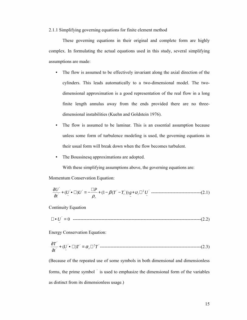
2.1.1 Simplifying governing equations for finite element method

These governing equations in their original and complete form are highly

complex. In formulating the actual equations used in this study, several simplifying

assumptions are made:

• The flow is assumed to be effectively invariant along the axial direction of the

cylinders. This leads automatically to a two-dimensional model. The two-

dimensional approximation is a good representation of the real flow in a long

finite length annulus away from the ends provided there are no three-

dimensional instabilities (Kuehn and Goldstein 1976).

• The flow is assumed to be laminar. This is an essential assumption because

unless some form of turbulence modeling is used, the governing equations in

their usual form will break down when the flow becomes turbulent.

• The Boussinesq approximations are adopted.

With these simplifying assumptions above, the governing equations are:

Momentum Conservation Equation:

'2'''''

'

))(1()(−−−

∇+−−+∇−=∇•+∂

∂ UgTTPUUt

Urr

r

υβρ

---------------------------------(2.1)

Continuity Equation

0' =•∇−

U -------------------------------------------------------------------------------------(2.2)

Energy Conservation Equation:

'2'''

'

)( TTUtT

r ∇=∇•+∂∂

−α -------------------------------------------------------------------(2.3)

(Because of the repeated use of some symbols in both dimensional and dimensionless

forms, the prime symbol ' is used to emphasize the dimensional form of the variables

as distinct from its dimensionless usage.)

16

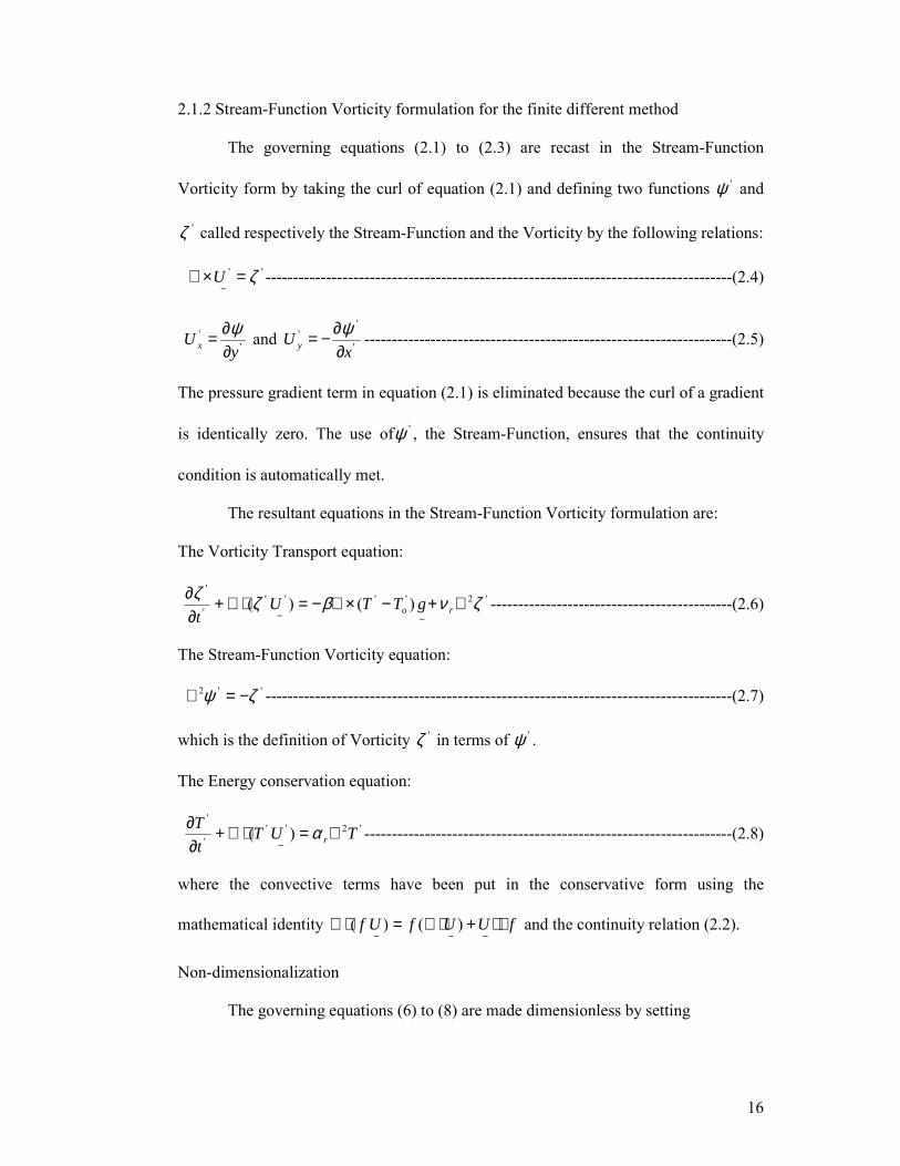
2.1.2 Stream-Function Vorticity formulation for the finite different method

The governing equations (2.1) to (2.3) are recast in the Stream-Function

Vorticity form by taking the curl of equation (2.1) and defining two functions 'ψ and

'ζ called respectively the Stream-Function and the Vorticity by the following relations:

'' ζ=×∇−

U -------------------------------------------------------------------------------------(2.4)

'

''

'' and

xU

yU yx ∂

∂−=∂∂= ψψ -------------------------------------------------------------------(2.5)

The pressure gradient term in equation (2.1) is eliminated because the curl of a gradient

is identically zero. The use of 'ψ , the Stream-Function, ensures that the continuity

condition is automatically met.

The resultant equations in the Stream-Function Vorticity formulation are:

The Vorticity Transport equation:

'2'''''

'

)()( ζνβζζ ∇+−×∇−=⋅∇+∂∂

−− ro gTTUt

--------------------------------------------(2.6)

The Stream-Function Vorticity equation:

''2 ζψ −=∇ -------------------------------------------------------------------------------------(2.7)

which is the definition of Vorticity 'ζ in terms of 'ψ .

The Energy conservation equation:

'2'''

'

)( TUTtT

r ∇=⋅∇+∂∂

−α -------------------------------------------------------------------(2.8)

where the convective terms have been put in the conservative form using the

mathematical identity fUUfUf ∇⋅+⋅∇=⋅∇−−−

)()( and the continuity relation (2.2).

Non-dimensionalization

The governing equations (6) to (8) are made dimensionless by setting

17

rrroi

or LLUU

TTTTT

Ltt

Lxx

αζζ

αψψ

αα 2''

'

''

''

2

''

,,,,, ===−−

=== −

−

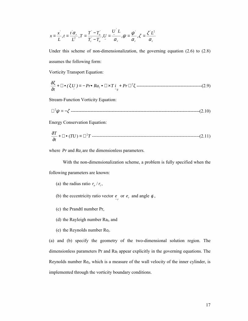
Under this scheme of non-dimensionalization, the governing equation (2.6) to (2.8)

assumes the following form:

Vorticity Transport Equation:

ζ∇+×∇••−=ζ•∇+∂ζ∂

−−

2PriTRaPr)U(t g

l -------------------------------------------(2.9)

Stream-Function Vorticity Equation:

ζψ −=∇ 2 -------------------------------------------------------------------------------------(2.10)

Energy Conservation Equation:

TTUtT 2)( ∇=•∇+

∂∂ -----------------------------------------------------------------------(2.11)

where lRaPr and are the dimensionless parameters.

With the non-dimensionalization scheme, a problem is fully specified when the

following parameters are known:

(a) the radius ratio io rr / ,

(b) the eccentricity ratio vector r

e−

or re and angle φ ,

(c) the Prandtl number Pr,

(d) the Rayleigh number Ral, and

(e) the Reynolds number Rel.

(a) and (b) specify the geometry of the two-dimensional solution region. The

dimensionless parameters Pr and Ral appear explicitly in the governing equations. The

Reynolds number Rel, which is a measure of the wall velocity of the inner cylinder, is

implemented through the vorticity boundary conditions.

18

2.2 Coordinate system for finite difference method

For the eccentric cases in the finite difference method, the bipolar coordinate

system, which is a more convenient coordinate system, is adopted. The Bipolar

coordinate system gives a fine mesh around the inner cylinder. The proved to be

essential for the accurate evaluation of temperature gradient in the heat flux calculation.

However, the Bipolar coordinate system can’t be used for the concentric cases owing to

singularity at 0=re . A Polar coordinate system is therefore employed for the

concentric cases.

2.2.1 Concentric geometry

The transformation between the Cartesian x-y coordinate system and the r-θ

Polar coordinate system is given by the following relations:

θθ sin,cos ryrx == )20(),0( πθ ≤≤∞<≤ r ---------------------------------------(2.12)

The governing equations in the θ−r coordinate system are:

)cos(sinPrPr)(1)( 2

θθθζζζ

θζζ

θ ∂∂+

∂∂⋅+∇=+

∂∂+

∂∂+

∂∂ T

rrTRal

rUU

rU

rtr

r -----(2.13)

ζϕ −=∇ 2 -----------------------------------------------------------------------------------(2.14)

TrTUTU

rTU

rtT r

r2)(1)( ∇=+

∂∂+

∂∂+

∂∂

θθ---------------------------------------------(2.15)

where r

Ur

U r ∂∂−=

∂∂= ψ

θψ

θ,1 and ).11( 2

2

22

22

rrrr ∂∂+

∂∂+

∂∂≡∇

θ

2.2.2 Eccentric geometry

The transformation between the Cartesian x-y coordinate system and the

Bipolar ηξ − coordinate system is given by the following relations:

)cos/(coshsincy)cos/(coshsinhcx

ξ−ηξ=ξ−ηη=

)( ∞<<−∞ η )20( πξ ≤≤ ------------------------------(2.16)

19

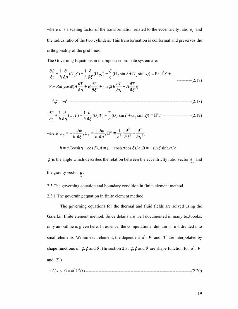
where c is a scaling factor of the transformation related to the eccentricity ratio re and

the radius ratio of the two cylinders. This transformation is conformal and preserves the

orthogonality of the grid lines.

The Governing Equations in the bipolar coordinate system are:

)](sin)([cosPr

Pr)sinhsin()(1)(1 2

ξηφ

ξηφ

ζηξζζξ

ζη

ζηξξη

∂∂−

∂∂+

∂∂+

∂∂•

+∇=+−∂∂+

∂∂+

∂∂

TATBTBTARal

UUc

Uh

Uht

----------(2.17)

ζψ −=∇ 2 ------------------------------------------------------------------------------------(2.18)

TUUcTTU

hTU

htT 2)sinhsin()(1)(1 ∇=+−

∂∂+

∂∂+

∂∂ ηξ

ξη ηξξη --------------------(2.19)

where )(1,1,12

2

2

2

22

ηξηψ

ξψ

ξη ∂∂+

∂∂≡∇

∂∂=

∂∂−=

hhU

hU

cBcAch /sinhsin,/)coscosh1(),cos/(cosh ηξξηξη −=−=−=

φ is the angle which describes the relation between the eccentricity ratio vector r

e−

and

the gravity vector −g .

2.3 The governing equation and boundary condition in finite element method

2.3.1 The governing equation in finite element method

The governing equations for the thermal and fluid fields are solved using the

Galerkin finite element method. Since details are well documented in many textbooks,

only an outline is given here. In essence, the computational domain is first divided into

small elements. Within each element, the dependent 'u , 'P and 'T are interpolated by

shape functions of θϕφ and , . (In section 2.3, θϕφ and , are shape function for 'u , 'P

and 'T )

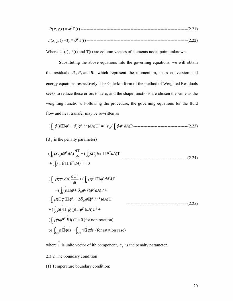
)(U),,(u i ttyx Ti φ= -------------------------------------------------------------------------(2.20)

20

)(P),,( ttyxP Tϕ= ---------------------------------------------------------------------------(2.21)

)(T),,( tTtyxT Tr θ=− -----------------------------------------------------------------------(2.22)

Where )(Ui t , P(t) and T(t) are column vectors of elements nodal point unknowns.

Substituting the above equations into the governing equations, we will obtain

the residuals 321 and , RRR which represent the momentum, mass conversion and

energy equations respectively. The Galerkin form of the method of Weighted Residuals

seeks to reduce these errors to zero, and the shape functions are chosen the same as the

weighting functions. Following the procedure, the governing equations for the fluid

flow and heat transfer may be rewritten as

P)(U))/((1

2

^

∫∫ ΩΩ−=+∇⋅ dAdAri T

piT

iT ϕϕεφδφϕ --------------------------------------(2.23)

( pε is the penalty parameter)

0T)(

T)u(T)( T

=∇⋅∇+

∇⋅+

∫

∫∫

Ω

ΩΩ

dAk

dACdtddAC

T

pT

p

θθ

θθρθθρ-----------------------------------------------(2.24)

case)ratation (for or

rotation)non (for 0T)(

U)))(((

U))/2((

P))/((

U)u(U)(

2

^

1

^

^

j^^

i22

2

^

iTi

1

∫∫

∫

∫

∫

∫

∫∫

Ω∂Ω∂

Ω

Ω

Ω

Ω

ΩΩ

⋅+⋅

=⋅

+∇⋅∇⋅+

⋅+∇⋅∇

++∇⋅−

∇⋅+

dsindsin

gi

dAji

dAr

dAri

dAdt

ddA

Y

T

Ti

T

Ti

T

φφ

ρβφθ

φφµ

φφδφφµ

ϕφδφ

φρφρφφ

-------------------------------------------(2.25)

where ^i is unite vector of ith component, pε is the penalty parameter.

2.3.2 The boundary condition

(1) Temperature boundary condition:

21

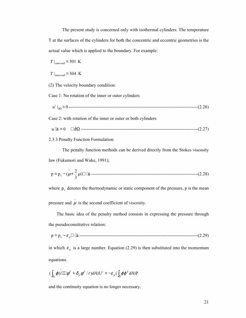
The present study is concerned only with isothermal cylinders. The temperature

T at the surfaces of the cylinders for both the concentric and eccentric geometries is the

actual value which is applied to the boundary. For example:

301| =outerwallT K

304| =innerwallT K

(2) The velocity boundary condition:

Case 1: No rotation of the inner or outer cylinders

0|u i =Ω∂ --------------------------------------------------------------------------------------(2.26)

Case 2: with rotation of the inner or outer or both cylinders

Ω∂∈=⋅ 0nu ------------------------------------------------------------------------------(2.27)

2.3.3 Penalty Function Formulation

The penalty function methods can be derived directly from the Stokes viscosity

law (Fukumori and Wake, 1991);

u)32(pp s ⋅∇+−=

−µµ -----------------------------------------------------------------------(2.28)

where sp denotes the thermodynamic or static component of the pressure, p is the mean

pressure and −µ is the second coefficient of viscosity.

The basic idea of the penalty method consists in expressing the pressure through

the pseudoconstitutive relation:

upp s ⋅∇−= pε -------------------------------------------------------------------------------(2.29)

in which pε is a large number. Equation (2.29) is then substituted into the momentum

equations.

P)(U))/((1

2

^

∫∫ ΩΩ−=+∇⋅ dAdAri T

piT

iT ϕϕεφδφϕ

and the continuity equation is no longer necessary.

22

2.4 Investigated geometric and physical parameters

2.4.1. Various parameters for the finite element method

In the present study, finite element method is applied to solve the primitive

variable form of the incompressible Navier-Stokes equations with Boussinesq

approximation. Therefore, the basic parameters:

1) rρ Reference density

2) β Coefficient of thermal expansion

3) 'rT Reference temperature

4) rυ Kinematic viscosity

5) rα Thermal diffusivity

2.4.2. Various parameters for the finite difference method

The vorticity-stream function formulation in the curvilinear coordinate system

is taken as the governing equation. Therefore, the system parameters:

1) The radius ratio irr /0 . ,5/0 =irr 2.6,/0 =irr 1.25/0 =irr are studied so that the

effects of the radius changes can reflect the correct results.

2) The eccentricity ratio vector−re .

−re =

L

e− =(

Le

Le vh , )

−re = 1/3, 2/3 is considered.

For the eccentricity ratio vector−re , L= irr −0 is the ‘mean’ clearance of the

annulus.

3) The Rayleigh parameterνα∆β=

3LTgRa'

l .

For the Rayleigh number, the strength of the buoyancy force relative to the viscous

force is disposed. From the formula it is seen that the Rayleigh number is

proportional to 'T∆ .

23

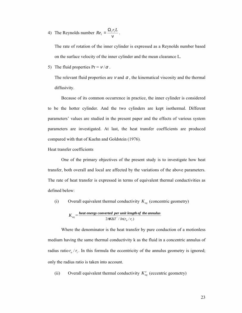
4) The Reynolds number ν

Ω=

LrRe iil .

The rate of rotation of the inner cylinder is expressed as a Reynolds number based

on the surface velocity of the inner cylinder and the mean clearance L.

5) The fluid properties Pr = αν / .

The relevant fluid properties are ν and α , the kinematical viscosity and the thermal

diffusivity.

Because of its common occurrence in practice, the inner cylinder is considered

to be the hotter cylinder. And the two cylinders are kept isothermal. Different

parameters’ values are studied in the present paper and the effects of various system

parameters are investigated. At last, the heat transfer coefficients are produced

compared with that of Kuehn and Goldstein (1976).

Heat transfer coefficients

One of the primary objectives of the present study is to investigate how heat

transfer, both overall and local are affected by the variations of the above parameters.

The rate of heat transfer is expressed in terms of equivalent thermal conductivities as

defined below:

(i) Overall equivalent thermal conductivity eqK (concentric geometry)

eqK =)/(/2 '

io rrInTK∆πannulusthe of length unit per convertedenergy heat

Where the denominator is the heat transfer by pure conduction of a motionless

medium having the same thermal conductivity k as the fluid in a concentric annulus of

radius ratio io rr / . In this formula the eccentricity of the annulus geometry is ignored;

only the radius ratio is taken into account.

(ii) Overall equivalent thermal conductivity eeqK (eccentric geometry)

24

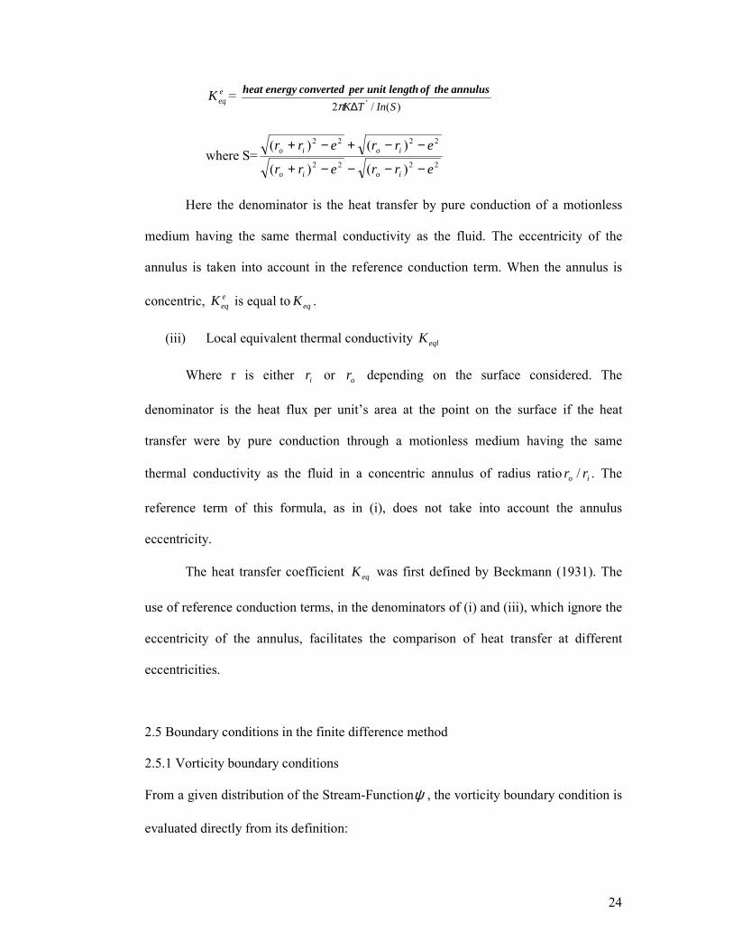
eeqK =

)(/2 ' SInTK∆πannulusthe of length unit per convertedenergy heat

where S=2222

2222

)()(

)()(

errerr

errerr

ioio

ioio

−−−−+

−−+−+

Here the denominator is the heat transfer by pure conduction of a motionless

medium having the same thermal conductivity as the fluid. The eccentricity of the

annulus is taken into account in the reference conduction term. When the annulus is

concentric, eeqK is equal to eqK .

(iii) Local equivalent thermal conductivity eqlK

Where r is either ir or or depending on the surface considered. The

denominator is the heat flux per unit’s area at the point on the surface if the heat

transfer were by pure conduction through a motionless medium having the same

thermal conductivity as the fluid in a concentric annulus of radius ratio io rr / . The

reference term of this formula, as in (i), does not take into account the annulus

eccentricity.

The heat transfer coefficient eqK was first defined by Beckmann (1931). The

use of reference conduction terms, in the denominators of (i) and (iii), which ignore the

eccentricity of the annulus, facilitates the comparison of heat transfer at different

eccentricities.

2.5 Boundary conditions in the finite difference method

2.5.1 Vorticity boundary conditions

From a given distribution of the Stream-Functionψ , the vorticity boundary condition is

evaluated directly from its definition:

25

wallwall |2ψζ −∇= ----------------------------------------------------------------------------(2.30)

Expression (2.30) in generalized orthogonal curvilinear coordinates and using the non-

slip flow condition at the wall of the cylinders, equation (2.30) becomes

)(112

2

2η

ξ

ηξη ηηψ

ηψζ

hh

hhhwall ∂∂

∂∂+

∂∂−= ----------------------------------------------------(2.31)

where η is constant along the wall and grid lines of constant ξ are perpendicular to the

wall. ξη hh and are the scale factors of the transformation.

(1) Concentric cylinders

For the concentric case, r and θ may be taken as ξη and respectively so that

1== rhhη and .rhh == θξ Equation (2.31) then becomes

wallwall rU

r|)( 2

2θψζ +

∂∂−= ------------------------------------------------------------------(2.32)

(2) Eccentric cylinders

For the eccentric case, from Appendix A, hchh =−== )cos/(cosh ζηηξ in the

Bipolar coordinate system. Equation (2.31) reduces to

wallwall h|1

2

2

2 ηψζ

∂∂−= ------------------------------------------------------------------------(2.33)

2.5.2 Stream-function boundary conditions

The Stream Function value oψ on the outer cylinder may be arbitrarily set to

zero. In the present study iψ is determined using the criterion that the pressure

distribution in the solution region is a single-valued function. Similar criteria were used

by Launder and Ying (1972) and Lewis (1979) for the numerical studies of isothermal

flows in non-simply connected geometries. Mathematically, this criterion implies that

the line integral of the pressure gradient sP

∂∂ along any closed loop circumscribing the

26

inner cylinder is zero i.e. ∫ =∂∂ .0ds

sP

sP

∂∂ can be evaluated from the momentum

conservation equations. The numerical implementation of this criterion is described in

the next chapter. The Stream-Function boundary conditions for both the concentric and

eccentric geometries are of the Dirichlet type as follows:

0| =outerwallψ ----------------------------------------------------------------------------------(2.34)

iinnerwall ψψ =| --------------------------------------------------------------------------------(2.35)

2.5.3 Temperature boundary conditions

The present study is concerned only with isothermal cylinders. The

dimensionless temperature T at the surfaces of the cylinders for both the concentric and

eccentric geometries is as follows:

0| =outerwallT

1| =innerwallT

27

CHAPTER 3 NUMERICAL SOLUTIONS

The finite difference method and finite element method were adopted to solve

the governing equations.

The finite difference method is a well-known method for solving the partial

differential equations. A good introduction to this method may be found in Ames

(1978). The practical applications of the method to problems in incompressible and

compressible fluid dynamics are described in great details in the very important work

of Roache (1972).

It is difficult for the finite difference method to solve the vorticity-stream

function formation with the moving boundary condition. Some special approaches such

as the single value condition are proposed to deal with the problem. Therefore, in the

present study finite element method is applied to solve the primitive variable form of

the incompressible Navier-Stokes equations with Boussinesq approximation.

The finite element method (FEM) is a numerical technique to obtain

approximate solutions to a wide variety of engineering problems. Although originally

developed to study the stresses in frame structures, it has since been extended and

applied to the broad field of engineering. The basic idea about the finite element

method can be found in Heinrich and Pepper (1999).

3.1 The finite-difference and finite-element approaches

3.1.1 The finite-difference method

Separate computer programs were written for the concentric and the eccentric

geometries. The system of mesh used in each case is the one natural to the particular

coordinate system.

28

Second-order accurate finite difference approximations were used for the

discretization of the governing equations whenever possible. The finite difference form

of equations (2.13) to (2.15) for the concentric and equations (2.17) to (2.19) for the

eccentric case were solved in a time-marching manner until satisfactory convergence

was attained. At each time the Stream-Function Vorticity equations must be solved to

convergence. Instead of second-order central differencing, upwind differencing was

used for the convective terms to obtain good stability.

3.1.2 The finite-element method

The basic idea of FEM is that a solution can be analytically modeled or

approximated by replacing it with an assemblage of discrete elements. Since these

elements can be put together in a variety of ways, they can be used to represent

exceedingly complex shapes. The FE discretization procedures reduce continuum

problems to one of a finite number of unknowns by dividing the solution region into

elements and expressing the unknown field variable in terms of assumed approximating

functions (or interpolation functions) within each element. The interpolation functions

(or shape functions) are defined in terms of the values of the field variables at specified

points called nodes (nodal points). The nodal values of the field variable and the

interpolation functions for the elements completely define the behavior of the field

variable within the elements. Once the nodal values are found, the interpolation

functions define the field variable throughout the assemblage of elements.

3.2 The solution procedure

3.2.1 The finite difference method

The solution process begins with the establishment of the necessary initial

values for ψζ , and T at time t=0. Other necessary parameters or constants that are

29

repeatly used in the program are also computed. The governing equations are solved in

a cyclic manner.

At the beginning of any particular cycle the time is increased by t∆ and the

distribution of ζ at the new time t=t+ t∆ is found by solving the Vorticity Transport

equation with boundary conditions obtained from the last known distribution of ψ .

With ζ known at all the interior points, the Stream-Function Vorticity equation is

solved in an iterative manner. The boundary value of ψ on the outer cylinder is always

zero. On the inner cylinder, iψ is found through an iterative procedure. From the latest

distribution of ψ , the velocity terms required in the convective terms of the Energy and

the Vorticity Transport equations are calculated. The next step in the cycle is to solve

the Energy equation for the temperature distribution T. Local and overall heat fluxes

may be calculated from the temperature distribution. The last step is to check if the

distributions ψ and T have converged and the energy balance is satisfactory. The

above cycle is repeated with increment in time t until the convergence criteria are met.

3.2.2 The finite element method

There are in general four different routes leading to a FE formulation: direct

approach, variational principle approach, weighted residual approach, and energy

balance approach. The advantage of the direct approach is that an understanding of the

techniques and essential concepts is gained without much mathematical manipulation.

But it can be used only for relatively simple problems. The variational principle relies

on the calculus of variations and involves extremizing a functional. Weighted residuals

approach has an advantage because it becomes possible to extend FEM to the problems

where no functional is available. The most applicable weighted residual approach is

Galerkin’s method. Regardless of the approach used to find the element properties, the

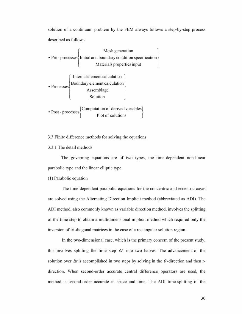
30

solution of a continuum problem by the FEM always follows a step-by-step process

described as follows.

•input properties Materials

ionspecificatcondition boundary and InitialgenerationMesh

processes-Pre

•

SolutionAssemblage

ncalculatioelement Boundary ncalculatioelement Internal

Processes

•solutions ofPlot

variablesderived ofn Computatioprocesses-Post

3.3 Finite difference methods for solving the equations

3.3.1 The detail methods

The governing equations are of two types, the time-dependent non-linear

parabolic type and the linear elliptic type.

(1) Parabolic equation

The time-dependent parabolic equations for the concentric and eccentric cases

are solved using the Alternating Direction Implicit method (abbreviated as ADI). The

ADI method, also commonly known as variable direction method, involves the splitting

of the time step to obtain a multidimensional implicit method which required only the

inversion of tri-diagonal matrices in the case of a rectangular solution region.

In the two-dimensional case, which is the primary concern of the present study,

this involves splitting the time step t∆ into two halves. The advancement of the

solution over t∆ is accomplished in two steps by solving in the θ -direction and then r-

direction. When second-order accurate central difference operators are used, the

method is second-order accurate in space and time. The ADI time-splitting of the

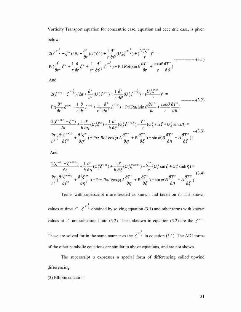
31

Vorticity Transport equation for concentric case, equation and eccentric case, is given

below:

)cos(sinPr)11Pr(

)()(1)(/)(2

21

2

2

22

2

21

21

θθθζ

θζζ

ζζθ

ζζζ θ

∂∂+

∂∂⋅+

∂∂+

∂∂+

∂∂

=+∂∂+

∂∂+∆−

+

++

nnnnn

unn

rnnu

nnr

unn

Trr

TRalrrrr

rUU

rU

rt

---------------(3.1)

And

)cos(sinPr)11Pr(

)()(1)(/)(2

21

2

2

211

2

2

121

121

1

θθθζ

θζζ

ζζθ

ζζζ θ

∂∂+

∂∂⋅+

∂∂+

∂∂+

∂∂

=+∂∂+

∂∂+∆−

+++

+++++

nnnnn

unn

rnnu

nnr

unn

Trr

TRalrrrr

rUU

rU

rt

----------(3.2)

)](sin)([cosPr)(Pr

)sinhsin()(1)(1)(2

2

2

2

5.02

2

5.05.0

ξηφ

ξηφ

ηζ

ξζ

ηξζζξ

ζη

ζζηξξη

∂∂−

∂∂+

∂∂+

∂∂•+

∂∂+

∂∂

=+−∂∂+

∂∂+

∆−

+

++

nnnnnn

nnn

nnu

nnunn

TATBTBTARalh

UUc

Uh

Uht

--(3.3)

And

)](sin)([cosPr)(Pr

)sinhsin()(1)(1)(2

2

12

2

5.02

2

5.015.01

ξηφ

ξηφ

ηζ

ξζ

ηξζζξ

ζη

ζζηξξη

∂∂−

∂∂+

∂∂+

∂∂•+

∂∂+

∂∂

=+−∂∂+

∂∂+

∆−

++

++++

nnnnnn

nnn

nnu

nnunn

TATBTBTARalh

UUc

Uh

Uht

(3.4)

Terms with superscript n are treated as known and taken on its last known

values at time nt . 21

+nζ obtained by solving equation (3.1) and other terms with known

values at nt are substituted into (3.2). The unknown in equation (3.2) are the 1+nζ .

These are solved for in the same manner as the 21

+nζ in equation (3.1). The ADI forms

of the other parabolic equations are similar to above equations, and are not shown.

The superscript u expresses a special form of differencing called upwind

differencing.

(2) Elliptic equations

32

Equation of the concentric case is solved with the Strongly Implicit Procedure

of Stone (abbreviated to SIP) introduced by H.L.Stone (1968). A series of ten

acceleration parameters generated by the method given in was used. The number ten

was arbitrarily selected.

One of the important merits of the SIP is that the rate of convergence is not so

sensitive to the choice of acceleration parameters. This means that suitable parameters

can be more easily and reliably estimated from the coefficient matrix than say in the

corresponding ADI method which requires accurate knowledge of the minimum

eigenvalues of a certain coefficient matrix to obtain good convergence rate.

For the eccentric configuration, the ADI method was favored because the

eigenvalues are allowed to be computed theoretically. See Birkhoff et al (1962) section

9 on the Helmholtz Equation in a rectangle. The Wachspress parameters, which are the

sequence of acceleration parameters used, can hence be obtained with great accuracy.

3.3.2 Boundary conditions

This section describes the numerical implementation of the boundary conditions

stated before. The boundary conditions are all of the Dirichlet type.

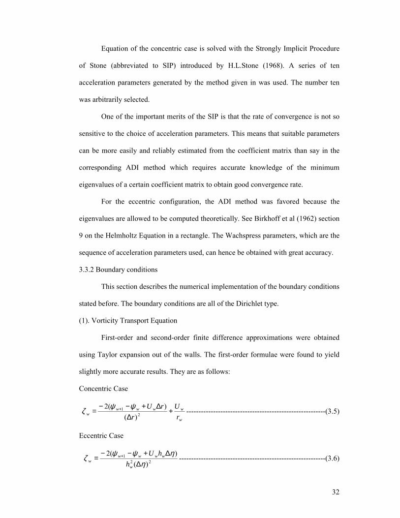
(1). Vorticity Transport Equation

First-order and second-order finite difference approximations were obtained

using Taylor expansion out of the walls. The first-order formulae were found to yield

slightly more accurate results. They are as follows:

Concentric Case

w

wwwww r

Ur

rU+

∆∆+−−

= +2

1

)()(2 ψψζ ---------------------------------------------------------(3.5)

Eccentric Case

221

)()(2

ηηψψζ

∆∆+−−

= +

w

wwwww h

hU------------------------------------------------------------(3.6)

33

where subscript w and w+1 refer to the values of the variables at the wall and one mesh

point away from the wall (in the fluid) respectively. wU is the tangential velocity of the

wall, which in the case of the outer cylinder wall is zero. The wU is determined from

the Reynolds number Rey1.

(2). Stream-Function Vorticity Equaiton

0=oψ

fi S=ψ

Assuming that a projected or guessed value of iψ called S is given, the

following steps are used to find a maxP∆ (maximum pressure difference term)

associated with S. This is done by first solving the equation ζψ −=∇ 2 with Si =ψ

and .0=oψ From the solution ψ , the pressure gradient terms θ∂

∂P (concentric case) or

ξ∂∂P are computed at all the interior points using the Momentum Balance equation (2.1)

in the respective coordinate systems. By integrating θ∂

∂P or ξ∂

∂P along all the closed

circumferential loops of constant r or η respectively (from πξθξθ 20 ==== to ), the

pressure difference terms of sP '∆ at all the loops are determined. A P∆ , among the

sP '∆ , which has maximum absolute value is selected as maxP∆ i.e. maxP∆ = P∆ such

that ≥∆ || P the absolute value of any sP '∆ .

A series of such S called ⋅⋅⋅⋅,,, 321 SSS etc. are projected at each time step and

their associated maxP∆ called ⋅⋅⋅∆∆∆ ,,, 3max

2max

1max PPP are computed. The first value 1S in

each time step is projected from Stream Function values 21 −− ni

ni andψψ at the previous

two time-steps. Depending on whether 1S is considered too high or too low a projection

34

(this can be seen from the sign of 1maxP∆ ), 2S is projected linearly from the relation

.||21|| 1

112−−=− n

iSSS ψ Subsequent values say lS are obtained by linear

interpolation between one pS and one qS (p,q<l) whereby pS has negative pPmax∆ and

qS has positive qPmax∆ ; both being of minimum absolute values in their respective sign

categories. In this manner a fS with almost minimum absolute || maxP∆ is obtained

after a sufficient number of projections are made and a convergence criterion applying

to consecutive value of the projection is satisfied. fS is then the value of iψ at time

step nt .

It would be very time-consuming if the Poisson equation ζψ −=∇ 2 is solved

for every projected value of iψ at each time step. Fortunately, by the linearity of the

equation, we need to solve ζψ −=∇ 2 only once at each time step. Using linear

superposition, if 'ψ is the solution to ζψ −=∇ 2 with 1Si =ψ , the solution to

ζψ −=∇ 2 with 2Si =ψ can be obtained by adding "12 )( ψSS − to 'ψ where "ψ is the

solution to the Laplace equation 02 =∇ ψ with 0.1=iψ . Solution to the last equation

are trivial in both coordinate system.

(3). Energy Equation

The two cylinders are maintained at isothermal condition, that is

0.1=iT and 0.0=oT

(4). Progressive built-up of boundary conditions

Solution can become unstable if the full value of a boundary condition is

suddenly imposed. To give a more gradual and stable start, temperature and velocity

boundary conditions are imposed over a number of time steps. The number of steps is

35

roughly proportional to the value of the boundary condition. The final solution is

independent of the number of steps used to introduce the boundary condition.

3.3.3 Convergence criteria

(1). Convergence of the inner iterations

Concentric case

For the concentric case where the SIP is used, a ‘Residue’ term ijsRe is defined

at each interior point as follows:

kijD

nij

kijs ψζ 2Re ∇+= ------------------------------------------------------------------------(3.7)

where ijD ∇ stands for the second-order finite difference operator of the Laplacian, n is

the global iteration number or time step and k is the inner iteration number. kijsRe is a

direct measure of the lack of convergence of kψ . The Stream Function distribution kψ

is considered to have converged sufficiently when

Nsrs

nrs

kij /]||[0005.0Re ∑< ζ ----------------------------------------------------------------(3.8)

for all interior points (i,j). N is the total number of interior points. In words, this means

that the residue at each interior point must be less than 0.0005 times the average

absolute vorticity value.

Eccentricity Case

Because the Stream Function frequently attains values close to zero, the

criterion that

δψψψ ≤≤≤≤−−−−++++ ||/|| kij

kij

kij

1 ------------------------------------------------------------------------(3.9)

(where δ is a small real number) holds at all interior points (i,j) is not practical. An

alternative criterion is used which involves first finding kpq∆ , the maximum absolute

36

difference between successive iterates kψ and 1+kψ , and the grid point (p,q) where is

occurs:

||max 1

),(

kij

kijji

kpq ψψ −=∆ + --------------------------------------------------------------------(3.10)

The criterion for the convergence of the inner iterations is that

0001.0)/|]|/([ <∆ ∑rs

krs

kpq Nψ --------------------------------------------------------------(3.11)

i.e. the maximum deviation between successive iterates is less than 0.0001 times the

average absolute Stream Function value. This criterion is satisfactory as long as ψ is a

reasonably well-behaved function which does not have highly localized peak values.

(2). Overall convergence

A run is deemed to have converged sufficiently when the following three

criteria are met:

a) 001.0)/|]|/([ <∆ ∑rs

nrs

npq Nψ

b) 001.0/|| 1 <−+ nij

nij

nij TTT

at all interior points (i,j).

c) 985.0/ ≥io QQ

where Q stands for heat flux through the cylinders.

The convergence of the Vorticity distribution is not included as a convergence

criterion because it is directly related to the Stream Function through its definition. The

convergence of the Stream Function ψ implies the convergence of the vorticity

distribution through the criterion may be different.

The degree of heat balance is included as a convergence criterion because it is a

fairly good barometer of the accuracy of the solution and the sufficiency of the mesh

size. It was found that the temperature solution usually converged more slowly than the

37

Stream Function. The exceptions were runs at high Reyleigh numbers where the lack of

convergence of the Stream Function indicated the presence or onset of flow instability.

It is not always possible to satisfy the heat balance criterion though qualitatively

it is clear the solution has already converged to a far greater extent than required by

both criteria (a) and (b). This happens predominantly in cases where the inner cylinder

is moved eccentrically downwards. In these cases, the mesh at the top of the annulus is

very coarse, while at the same time the temperature gradient at the top of the outer

cylinder is very high because of the impinging thermal plume. For such cases, even

interpolation is not sufficient to resolve the extremely high gradient encountered.

3.4 Finite element methods for solving the equations

3.4.1 The details solving procedures

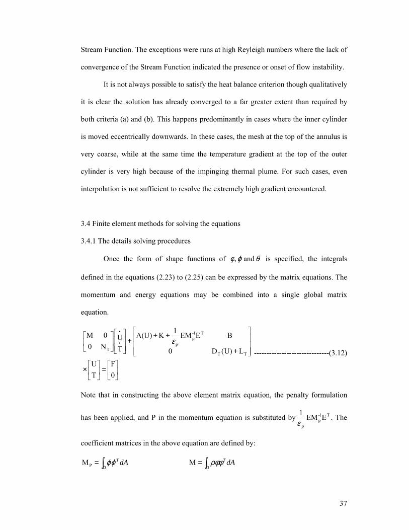
Once the form of shape functions of θϕφ and , is specified, the integrals

defined in the equations (2.23) to (2.25) can be expressed by the matrix equations. The

momentum and energy equations may be combined into a single global matrix

equation.

=

×

+

+++

•

•

0F

TU

LU)(D0

BEEM1KA(U)

TU

N00M

TT

T1-p

pT

ε ------------------------------(3.12)

Note that in constructing the above element matrix equation, the penalty formulation

has been applied, and P in the momentum equation is substituted by T1-p EEM1

pε. The

coefficient matrices in the above equation are defined by:

∫Ω= dATϕϕPM ∫Ω= dATρφφM

38

∫Ω ∇⋅∇= dAk TθθTL ∫Ω ∇⋅= dAC pT

T uU)(D θθρ

∫∫ ΩΩ∇⋅∇⋅+⋅+∇⋅∇= dAjidAr T

ijT

iT ))(())/2((K

^^2

2ij φφµδφφδφφµ

∫Ω= dAC TpθθρTN ∫Ω +∇⋅= dAri T

i ϕφδφ )/(E 2

^

i

∫Ω ∇⋅= dATuA(U) φρφ ∫Ω ⋅= giT^

B ρβφθ

∫ Ω∂⋅= dsn F φτ

where U is a global vector containing all nodal values of u and v. The assembled global

matrix equations are stored in the skyline form and solved using the Gaussian

elimination method. The successive substitution method is applied for nonlinear

iteration and the time derivatives are approximated using the implicit finite difference

scheme.

3.4.2 The shape function

The element can be chosen from any of the four node, eight node and nine node

elements (fig. 3.1.1). The shape function of quadrilateral elements (4-9) nodes may be

described in Table 3.1.

39

CHAPTER 4

ANALYSIS OF RESULTS FOR THE FINITE ELEMENT METHOD

The numerical results from the finite element method will be analyzed and

discussed in this chapter. The numerical model from the finite element method

produces the computational results of the velocity and temperature fields, which show

the detailed flow fields and temperature distributions.

The computational algorithm developed above is capable of predicting the

temperature distribution, the streamline distribution and internal convection in the

horizontal annular between two circular concentric or eccentric cylinders. A set of

computed results is shown for air, whose physical properties are given in Table 4.1.

The mesh independence testing procedure for the computation is considered here and

the final mesh used for the computation is determined so that any further refinement of

the mesh produces an error smaller than 0.1%. Finally, 221 nine-node elements are

adopted to calculate the thermal and fluid flow for half mode, which is used to simulate

the natural convection without both inner and outer cylinders’ rotation, and 578 nine-

node elements for whole mode with the cylinders rotating. The penalty formulation is

used for the pressure field computation. A convergence criterion of 1×10-3 is set for

relative error associated with unknowns for temperature and velocity fields.

The effects of Rayleigh number, radius ratio and eccentric ratio on the flow and

heat transfer are separately discussed in sections 4.1, 4.2 and 4.3. Section 4.4 and 4.5

emphasized the effect of the rotation. Section 4.4 focuses on the effect of rotating the

inner, outer and both cylinders between the concentric cases and section 4.5 is set for

the eccentric cases. The air is selected as the working fluid, which is used for the

numerical studies of the present investigation. The present finite element method is

40

validated by comparing its numerical results with the available data in the literature and

very good agreement has been achieved.

41

4.1 The effect of Rayleigh numbers

The effect of different Rayleigh number is shown in Fig 4.1.1 – 4.1.5. Half

model is adopted given the symmetry of the concentric annuli. In Fig. 4.1.1, a

symmetric pair of counter-rotating kidney is set in the annuli. However, the temperature

distribution (see Fig. 4.1.1(a)) seems like that of the natural convection from a heated

circular cylinder. The temperature contour suggests that thermal transport in the annuli

is primarily due to conduction. Temperature inversion appears to occur when the

Rayleigh number is above 104. Fig. 4.1.2-4.1.5 show that the inversion is gradually

becoming greater with increasing Rayleigh number.

There are two approaches to increase Rayleigh number, enlarging the radius of

cylinders or temperature difference between inner and outer cylinders. Fig. 4.1.2 and

4.1.3 separately depict the temperature, streamline and velocity at the Rayleigh number

of 9×104. Compared with each other, little difference is found so that Rayleigh number

is the major parameter in the low Rayleigh number.

The section also discussed when the unstable flow set in as a form of two-

dimensional oscillatory flow about the longitudinal axis. The numerical solution is

reasonable in Rayleigh number of 3.09×105. However, the streamline plots and the

temperature contours yield oscillation, therefore, there is some hint that the unstable

flow appears. When the Rayleigh number is 3.85×105, one zero streamline is yielded in

the old stagnant area. It may be deduced that for Rayleigh numbers about 1.1×105, the

time-averaged flow behavior and heat transfer of the actual physical flow between the

two cylinders are not very different from those of a hypothetical two-dimensional flow

without the oscillatory motion, and this lends credence to the possibility that the

numerical method may yet yield a reasonable solution. From Fig. 4.1.4 and Fig. 4.1.5,

42

the highly distorted form of the isotherms and streamlines manifests the unstable nature

of the flow at so high Rayleigh numbers.

The experimental investigation of Powe et al. (1969) described that for radius

ratios greater than about 1.8, instability at high Rayleigh number initially sets in as a

form of two-dimensional oscillatory flow about the longitudinal axis. The flow in a

plane perpendicular to the longitudinal axis exhibits the same kidney-shaped pattern

and the patterns in adjacent planes oscillates out of phase with each other resulting in

an apparent wave motion along the axis of the annulus. At the Rayleigh number of

5103× , these oscillations were still only intermittent and presumably of small

amplitude. Above the Rayleigh number of about 6105.1 × there was no definite

frequency in the oscillation and the plume became turbulent at the Rayleigh number of

about 7102 × .

In present the numerical results show that unstable phenomena began to be

yielded between Rayleigh number 3.09×105 and 3.85×105. One circular flow at the

stagnation area of the low Rayleigh number is shown from Fig. 4.1.5 (c). The present

numerical results agree well with experimental results obtained by Powe et al.

4.2 The effect of the radius ratio

This section focuses on the effect of the radius ratio. This part only emphasizes

the effect of the radius ratio of 2.6 and 5.0 from the finite element method in the high

Rayleigh number. The computed results for radius ratio of 2.6 and 5.0 are shown in Fig.

4.2.1 – 4.2.2.

The radius ratio has a significant effect on the flow and temperature distribution

between horizontal cylinders. Fig. 4.2.1 depicted temperature and flow fields of radius

ratio 2.6 and 5.0 cases at the Rayleigh number of 1.5×105. From Fig. 4.2.1 (b) and (e),

43

the center of kidney cell moved down and the stagnant zone becomes larger when the

radius ratio is enlarged from 2.6 to 5.0 at the same Rayleigh number.

It is easy for the higher radius ratios to yield temperature inversion. In

comparison of computed results between Figure 4.2.1 (a) and (d) it is apparent that the

higher radius ratio has a relatively greater temperature inversion. The stagnant

temperature zone is increased further for the larger radius ratios of 5.0. The major

reason is the boundary layer flow at high radius ratios has a higher momentum which

enables it easily to distort the isotherms to create the effect of temperature inversion.

The main conclusion is that the convective heat transfer is favored at higher radius

ratio. The convective flow around the inner cylinder increases rapidly as the radius ratio

is increased.

The instability of the two-dimensional oscillatory type sets in at higher Rayleigh

number for higher radius ratio. From Figure 4.2.2 (b), the strong oscillation appears

between the two horizontal cylinders, however, the temperature distribution has no

great change. Therefore, it may be deduced that for Rayleigh numbers between 5×105

and 1×106, the heat transfer of the actual convective flow between the two cylinders are

not different from those of a hypothetical two-dimensional flow without the oscillatory

motion, and this lends credence to the possibility that the finite element method may

yet yield a reasonable solution for the radius ratio 5.0.

4.3 The effect of eccentricity

The effects of eccentricity between the two horizontal cylinders were

numerically studied for eccentric ratio 0.75 and 0.5. In this case of a natural convection

in annulus between eccentric cylinders, the cylinder’s intracenter line is defined as the

line to connect the centers of the outer cylinder and the inner cylinder as shown in Fig.

44

1.1.1. For the case of eccentric ratio 0.75, Fig. 4.3.1 and 4.3.2 show that the

temperature and fluid flow between eccentric cylinders, which intracenter line is

parallel to the gravity vector. This case is very similar to the concentric case in such a

way that the flow is symmetric with respect to the intracentral line, and only half of the

field can be considered as the computational domain. The computational study of the

problem when the intracentral line is inclined with respect to the gravity vector is

relatively complicated so that Fig. 4.3.3 depicted two kinds of situation whose

intracentral line has degree 45o and –450 against the horizontal line.

The immediate effect of moving the inner cylinder upwards (Fig. 4.3.2) is to

enlarge the size of the stagnant zone and reduce the size of the of the kidney flow cell.

At high eccentric ratio 0.75, Fig. 4.3.2(b) depicted that one circular flow cell appeared

to occur at the bottom of the annuli and the kidney cell is squashed and connected to

the circular flow. In Fig. 4.3.2(a), the thermal plume is squashed to create a pair of

symmetrical humps. This indicates that the thermal boundary layer on the inner

cylinder has begun to separate from the cylinder before reaching the top of the annulus.

There is no district thermal plume as in other cases. A reduction of convective activities

can be expected. Moving the inner cylinder downwards (Figure 4.3.1) has the quite

opposite effect. The stagnant zone is reduced and convection is increased.

In Fig. 4.3.3, the Rayleigh number is about 4.95×104 and the eccentricity ratio is

0.5 with 6 k temperature difference between inner and outer cylinders. Figure 4.3.3 (a-

c) shows temperature, streamline and velocity plots for moving the inner cylinder to

angular 450 against the horizontal line, which has characteristics like that of moving the

inner cylinders both right and up. Fig. 4.3.4 (1) and (3) depict the temperature

distribution along the shortest and longest lines between the inner and outer cylinders

for the case moving the inner cylinder to angular 450 in the anti-clockwise direction.

45

Compared with the concentric case, the thermal plume is a little shifted to the left side

and reduced; the kidney shaped flow cell on the left side is enlarged and that on the left

side is squeezed to very small size; A large area where the temperature gradient is very

small appears in the left down side, which can be viewed in Fig. 4.3.3 (a) and found in

Fig. 4.3.4 (3). Corresponding to the small temperature gradient close to the center of

the left kidney cell, a small fluid flow is shown in the velocity plot in Fig. 4.3.3 (c).

Fig. 4.3.4 (1) describes the temperature distribution in the shortest distance line

between inner and outer cylinders, along which a sharp temperature gradient exists.

On the other hand, moving the inner cylinder to angular –450 produced a larger

thermal plume and smaller stagnation zone compared to that to angular 450. Fig. 4.3.4

(4) and (2) also shows separately a flat temperature distribution and a large

temperature gradient along the longest distance line and the shortest distance line

between inner and outer cylinders.

4.4 The effect of rotating the inner and/or outer cylinders between concentric cases

This section focuses on investigation of the effects of the rotation between

horizontal concentric cylinders, which include inner cylinder rotating, outer cylinder

rotating and both of them rotating in the same and opposite direction. The Rayleigh

number is kept 4.95×104 and the eccentricity ratio is 0.5 with the inner and outer

cylinders’ temperature being separately 307 K and 301 K. The tangential velocity is set

to 0.1 m/s for only one cylinder rotating and 0.05 m/s for both of them rotating. In this

section, the numerical results and the physics of the flow as revealed by the numerically

obtained streamline and isothermal plots and temperature distribution along the selected

lines are discussed.

46

The numerical results in Fig. 4.4.1, show pictorially the flow and temperature

fields when the inner cylinder is rotated (a-b) and the outer cylinder is rotated (c-d).

The rotation considered is both in the clockwise direction. The immediate effect of

rotating the inner cylinder is to cause the fluid adjacent to the surface of the rotating

cylinder to move with it by the virtue of viscous drag as clearly illustrated in Fig. 4.4.1

(b) and (d). For the non-rotating concentric case, the hot fluid adjacent to the inner

cylinder rise upwards because of its reduced density and then it is cooled at the top of

the annulus so that the cooled fluid falls sideways along the outer cylinder wall. When

the inner cylinder is rotated in the clockwise direction, the left-hand hot-fluid flow’s

velocity has the same velocity direction as the rotating cylinder. Therefore, the left-

hand cell is elongated in size while the right-hand cell is reduced for the inner rotating.

The circulation, defined as the integral ∫ ⋅ dsu , of the right-hand is thus reduced while

that in the left-hand is increased. On the other hand, rotating the outer cylinder in the

clockwise induces the right-hand cooled fluid with the same velocity direction

increasing so that it has a large right-hand cell and small left-hand cell. The isotherm

plots Fig. 4.4.1 (a) and (c) show that the thermal plume and the stagnant zone are

shifted in the direction of the rotating. Corresponding to the non-rotation case, the

thermal plume with the inner rotating is driven to an angular position of Φ = 800

(clockwise) from the highest point of the inner cylinder while the lower temperature

stagnant zone is only changed a little; the outer cylinder rotating caused the stagnant

zone approaching to Φ = 900 (clockwise) from the lowest point of the outer cylinder

with slightly shifted thermal plume, which is clearly depicted in Fig. 4.4.1 (a) and (c).

The temperature distribution along the line with different angle against the horizontal

line from the inner cylinder to the outer cylinder is shown in Figure 4.4.2. The higher

temperature along line 1 (Φ = 00) compared with the lower line 2 (Φ = 900) and the

47

nearly same temperature of line 3 and 4 numerically reveals the large thermal plume

shifting and small lower temperature stagnant zone shifting for inner cylinder rotating.

On the other hand, line 5, 6, 7 and 8 described the outer cylinder rotating case.

The effects of rotating both the inner and outer cylinders with the same and

opposite directions on the flow and heat transfer for the concentric configuration is

pictorially and numerically shown in Fig. 4.4.3 and 4.4.4. Fig. 4.4.3 (a-c) illustrate the

temperature, the streamline and the velocity with the same rotating direction, which

temperature distribution seems like that of only inner cylinder rotating except that the

low temperature stagnant zone move further away from the bottom part. The hot fluid

flow on the left-hand cell impinge into the right side with the help of the rotating inner

cylinder; the cooled fluid flow on the right-hand cell spreads around most area of the

outer cylinder (see Fig. 4.4.3 (b)). Lines 1-4 in Fig. 4.4.4 show the temperature

distribution along lines shooting from the inner to the outer cylinder with angular

position Φ = 00, 900, 1800 and 2700 against the horizontal line. Various parameters’ plot

for the inner and outer cylinder rotating in the opposite direction is shown in Fig. 4.4.3

(d-f). The root of the thermal plume dives into the right-hand part because of the drag

force from the rotating inner cylinder while the top of the thermal plume driven by the

viscosity of the rotating outer cylinder is shifted to the left-hand side. The low

temperature stagnant zone is moved slightly up to the right-hand. Fig. 4.4.3 (e) shows

that the left-hand cell is largely elongated that it will engulf the right cell because the

viscosity of both the inner and outer cylinders enlarges the left-hand cell.

4.5 The effect of rotating the inner and/or outer cylinders between eccentric cylinders

This section numerically simulates the natural convection in the annulus

between the vertically eccentric cylinders (the cylinder’s intracenter line is parallel to

48

the gravity vector) with both inner and outer cylinders rotating. The Rayleigh number is

kept at 4.95×104 and the inner and outer cylinders’ temperature is respectively at 307 K

and 301 K. The tangential velocity is set to 0.05 m/s for both of them rotating. Several

cases with different eccentric ratios (0.5 and 0.7) are discussed in the section. The close

proximity of the outer cylinder at the narrow throat exerts a great influence on the fluid

flow and temperature distribution in the annulus.

In the case of moving the inner cylinder up at the eccentric ratio of 0.5, the

narrowness of the throat region makes it difficult for the thermal plume to go through it.

Fig. 4.5.1 (a) and (d) respectively show the temperature of both cylinders rotating with

the same and opposite directions. Since the narrowness of the throat region reduces the

thermal plume, only the low temperature stagnant zone is moved left or right with the

outer cylinder rotating. Fig. 4.5.2 shows that the temperature along the shortest line and

longest shooting from the inner and outer cylinder with the same cylinders’ rotation

direction is similar to that with opposite direction. Therefore, the right-hand cell evaded

and occupied the stagnant zone when both cylinders rotate in the same direction and

shrank and left the stagnant zone when both cylinders rotate in the opposite direction. It

is interesting to note that the flow in the right-hand cell (see Fig. 4.5.1 (b)) is cut off

from the outer cylinder when the inner cylinder has different velocity as the outer

cylinder and the left-hand cell (see Fig. 4.5.1 (e)) is cut off from the inner cylinder

when both cylinders rotate in the same direction.

Similar temperature and fluid flow fields at the eccentricity ratio of 0.75 are

given in Fig. 4.5.3. The velocity of both inner and outer cylinder is 0.1 m/s. The narrow

throat plays a further important role on both the flow and temperature in the annulus.

From Fig. 4.5.3, the rotation of the outer cylinder exerts a great influence. Compared

with the results at the eccentricity ratio of 0.5, the faster rotated outer cylinder (0.1m/s)

49

associated with the further narrow throat decided the flow pattern. The inner cylinder is

set to rotate in the clockwise direction. If the outer cylinder rotates in the clockwise, the

right kidney cell will occupy the whole computed space except the small area close the

narrow throat. On the other hand, the anti-clockwise rotation of the outer cylinder

produces the opposite activities. Corresponding to the flow pattern, the low temperature

stagnant zone follows the rotation direction of the outer cylinder, which is shown in

Fig. 4.5.3 (a) and (d).

In the case of rotating the inner cylinder down at the eccentric ratio of 0.5,

moving the inner cylinder vertically down without rotation produces an increase in the

size of the rotating cells accompanied by a reduction in the size of stagnation zone. The

thermal boundary layer on the outer cylinder is increased in length from that of the

concentric case. When the rotation is applied to both cylinders, the out layer of the

thermal plume is moved with the outer cylinder and the root of the thermal plume is

shifted by the inner cylinder. The narrow throat is moved downwards, which reduces

the effect of the outer cylinder’s rotation and increases the influence of the inner

cylinder’s rotation because it is difficult for the particles of the cooled fluid driven by

the outer cylinder to pass the smaller stagnant part. The temperature and fluid flow

fields of both cylinders rotating in the same and opposite direction are respectively

presented in Figure 4.5.4 (a-c) and (e-f). Corresponding to Fig. 4.5.2, Fig. 4.5.5

numerically shows the temperature distribution along the shortest line and longest line

shooting from the inner cylinder to the outer cylinder.

50

CHAPTER 5

ANALYSIS OF RESULTS FOR THE FINITE DIFFERENCE METHOD

The chapter solves the numerical model through using finite difference method.

The numerical model from the finite difference method yields details of the flow and

the temperature fields through the streamline and isotherm plots and then computes the

local heat transfer values to predict the overall heat transfer coefficients. These plots

help to show the physics of the flow and the heat transfer behavior. All the isotherm

and streamline plots in this chapter are drawn by the software Tecplot 8.0, so that one

grid line can not be deleted because of the mesh divisions.

The overall heat transfer coefficients yielded by the numerical model at the

radius ratio of 2.6 are compared with similar results of other investigators. The good

agreement is a confirmation of the validity of the numerical model (see Fig. 5.0.1).

The effects of Rayleigh number, radius ratio and Reynolds number on the flow

and heat transfer between concentric cylinders are discussed in Sections 5.1, 5.2 and

5.3 respectively. Section 5.4 focuses on the heat transfer and fluid flow between

eccentric cylinders without inner cylinder rotating and Section 5.5 for eccentric

cylinders with inner cylinder rotating. In these sections, the discussions of the heat

transfer results are preceded by an analysis of the physics of flow as revealed by the

streamline and the isotherm plots. The working fluid with a Prandtl number of 0.701

(air) is assumed for the numerical studies of the present investigation.

51

5.1 The effects of Rayleigh numbers

At low Rayleigh numbers, the rate of convection of heat energy from the inner

cylinder to the outer cylinder is low because the buoyancy force proportional to the

temperature difference is very small and the induced flow velocity is low. At

2102×=lRa (Fig. 5.1.1 (a)), the isotherm plots are almost concentric circles like those

of pure conduction since the convective flow velocity is small. However, the counter-

rotating pair of kidney-shaped vortices (Fig. 5.1.2 (a)) is already clear. The overall heat

transfer coefficient for Rayleigh numbers up to just a few thousands is close to 1.0,

indicating that the heat transfer is predominantly conductive. Though the convective

flow exits at low Rayleigh numbers, the overall heat transfer is dominated by the

conduction. The temperature in the annuli falls monotonically, shooting outwards.

With the Rayleigh number increasing, the increased flow velocity on the

surfaces of both cylinders caused by the increased buoyancy results in the distortion of

the hitherto circle-like isotherms. At 410=lRa (Fig. 5.1.1 (c)), the isotherm plots have

lost its circular forms. As the Rayleigh number is increased to be strong enough, a

situation of temperature inversion occurs in which cooler fluid is separated from the

cooling surface by a layer of warmer fluid. The ‘extent’ of inversion is greater at higher

Rayleigh numbers. True boundary layer flow occurs for Rayleigh numbers above

4103× . As temperature inversion develops with increasing Rayleigh number, the shape

of a thermal plume begins to form at the top of the inner cylinder. By 4105× , a well-

defined thermal plume can be seen clearly (Fig. 5.1.1 (d)). The thermal plume becomes

narrower as the Rayleigh number is increased. The streamline plots of Fig. 5.1.2 reveals

that the kidney-shaped cells become progressively elongated and the center of rotation

move higher up though further increase in the Rayleigh number merely further

distorting the isotherms. At the Rayleigh number of 510 , the centers are about 030±

52

from the upward vertical. The thermal plume becomes narrower as the Rayleigh

number is increased. A pair of very weak counter-rotating cells is formed at the

stagnation zone of the bottom of the annulus. The effect is manifested by two additional

zero-valued streamlines. These cells are formed as more fluid is being drawn from the

sides of the annulus at high Rayleigh numbers.

The experimental investigation of Powe et al. (1969) manifested that for radius

ratios greater than about 1.8, instability at high Rayleigh number initially sets in as a

form of two-dimensional oscillatory flow about the longitudinal axis. The flow in a

plane perpendicular to the longitudinal axis exhibits the same kidney-shaped pattern

and the patterns in adjacent planes oscillates out of phase with each other resulting in

an apparent wave motion along the axis of the annulus. At the Rayleigh number of

5103× , these oscillations were still only intermittent and presumably of small

amplitude. Above the Rayleigh number of about 6105.1 × there was no definite

frequency in the oscillation and the plume became turbulent at the Rayleigh number of

about 7102 × . It may be deduced that for Rayleigh numbers between 510 and 610 , the

time-averaged flow behavior and heat transfer of the actual physical flow between the

two cylinders are not very different from those of a hypothetical two-dimensional flow

without the oscillatory motion, and this lends credence to the possibility that the

numerical method may yet yield a reasonable solution. From Fig. (5.1.1(f)) and Fig.

(5.1.2(f)), the highly distorted form of the isotherms and streamlines manifests the

unstable nature of the flow at so high Rayleigh numbers.

5.2 The effects of Radius ratio

This section focuses on the effects of radius ratio on the flow and the heat

transfer in concentric annulus for radius ratios up to 5.0. The higher radius ratios make

53

the effects of the outer cylinder so small that the flow and the heat transfer around the

inner cylinder would be almost close to those of a free convecting cylinder. The three

radius ratios of 1.25, 2.6 and 5.0 were investigated for the flow and temperature

distribution.

The radius ratio is one of the important parameters for measuring the heat

transfer and the flow between the horizontal annuli. When the radius is low, free

movement of the fluid is more difficult and the conductive mode of heat transfer

becomes dominant, whereas at the large radius ratios, the heat transfer from the inner

cylinder approaches that of natural convection from a heated horizontal cylinder.

The isotherm and streamlines for radius ratio of 1.25, 2.6 and 5.0 at various

Rayleigh numbers are described in Figs. 5.2.1-5.2.3 and in Figs. 5.1.1-5.1.2. For the

larger radius ratios and the smaller radius ratios, the convection and conduction

dominate the flow differently. Convective heat transfer which is dependent on the

velocity of the flow over the surface is suppressed at the small radius ratios (1.25)

because the proximity of the walls forces the opposite-direction flows on the two

cylinders to interact strongly with each other (through viscosity) and slow each other

down. Therefore, the isotherms remain more nearly circular up to a higher Rayleigh

number. At high radius ratios, the flows on the cylinders are separated by greater

distances and do not affect each other that the convection have a great effect. The

boundary layer flow at high radius ratios thus has a higher momentum which enables it

easily to distort the isotherms to create the effect of temperature inversion. It is thus

easy for the higher radius ratios to yield temperature inversion.

5.3 The effect of the inner cylinder rotating

54

The effects of the rotation of the inner cylinder on the flow and the heat transfer

in concentric annular spaces are the subjects of this section. The computed results are

for the radius ratios of 2.6, and as in the previous section, a Prandtl number Pr of about

0.7 is assumed. The actual numerical results and the physics of the flow as revealed by

the numerically obtained streamline and isotherm plots are discussed.

Figs. 5.3.1-5.3.2 show the streamline plots and the isotherm plots when the

inner cylinder is rotated with increasing speed at a fixed Rayleigh number of 4105.5 × .

The fluid adjacent to the surface of the inner cylinder moves with the inner cylinder for

the virtue of viscous drag yielded by the rotating inner cylinder. Rotating the inner

cylinder has the effect on rising the hot fluid on the ascending side of the cylinder while

on the descending side, the rising hot fluid is slowed down. Near the surface of the

inner cylinder on the descending side is a small region of very low flow velocity. The

effect of rotation on the flow field at the Reynolds number (Reyl=140) is depicted in

Fig. 5.3.1(a). The right-hand cell is elongated while the left-hand cell is reduced. The

circulation, defined as the integral ∫ −−⋅ dsU , of the left-hand is reduced while that in the

right-hand cell is increased. Since the zero-value streamline has lifted off the surface of

the inner cylinder, the thermal plume is shifted in the direction of the rotation which is

depicted in the isotherm plot Fig. 5.3.2 (a). The point of impingement on the outer

cylinder is correspondingly moved. The right-hand cell grows further in size while the

left-hand cell becomes smaller and weaker with increasing the angular speed to the

Reynolds number of 280. The left-hand cell is now separated from the inner cylinder.

Fig. 5.3.1 (b) showed that there is a zone of Couette-like flow around the inner

cylinder. Fig. 5.3.2 (b) depicted that the thermal plume has shifted even further in the

direction of rotation and its origin or ‘root’, the region near to the surface of the inner

cylinder where the thermal plume rises from, is lightly below the horizontal level of the

55

center of the inner cylinder. On the outer cylinder, the point of plume impinge has

shifted further down and temperature gradient has dropped.

With increasing Reynolds number, the right-hand cell elongates further as the

left-hand cell continues to shrink in size. When the Reynolds number rises to 416, the

right-hand cell is nearly close to its maximum length. Therefore, the growing ‘Couette-

flow’ region around inner cylinder encroached the cells. At the Reynolds number of

800 and 1120, the kidney-shaped eddy has been changed into a layer of very weak flow

pressed against the left-hand surface of the outer cylinder. At the Reynolds number of

1120, the ‘Couette-flow’ zone has stretched to a third of the clearance. This can been

seen in Fig. 5.3.1 (f).

The gradual disappearance of the thermal plume can be seen from the Fig. 5.3.2

(c) to 5.3.2 (f). The plume becomes less distinct and the ‘root’ of the plume, a region of

relatively low temperature gradient is extended when the Reynolds number is

increased. Therefore, this results in a rapid reduction of the temperature gradient around

the inner cylinder. From the Reynolds number of 560 to 800, increased numbers of

nearly circular rings of isotherms are formed around the inner cylinder. At the Reynolds

number of 1120, the isotherms away from the inner cylinder almost become circular,

and the temperature they represent is approaching that of pure conduction. However,

this situation is unlike in real flow because it is known that the two-dimensional

circular Couette flows at high Reynolds numbers are unstable.

5.4 The effects of eccentricity

Eccentricity has a great effect on the flow and heat transfer behavior in the

horizontal annulus. The flow field is in fact strongly influenced by the geometry of the

annulus as well as its orientation. The effects of eccentricity on the heat transfer were

56

studied at the radius ratios of 2.6 using the numerical model of the finite difference

method. The present study focuses on the eccentricities in the angular ±450 against the

horizontal direction.

The streamline and isotherm lines at the eccentricity ratios re of 1/3 and 2/3

and the radius ratio of 2.6 are depicted in Figs. 5.4.1-5.4.3. The Streamline plots

depicted that the immediate effect of moving the inner cylinder upwards is to yield a

reduction in the size of the two counter-rotating flow cells and to increase the size of

the stagnation region at the bottom of the annulus. The thermal boundary layer on the

outer cylinder is reduced in length from that of the concentric case. The increase of

conduction can be predicted. Moving the inner cylinder downwards has quite the

opposite effect. However, For eccentricity ratio 31≤re , the inner cylinder seem to be

unaffected by its own position. At the upward eccentricity )32,0(=

−re , the isotherm plots

depict that the isotherms around the inner cylinder yield a pair of symmetrical humps.

These indicate the inner thermal boundary layer has begun to separate from the cylinder

before reaching the top of the annulus. There is no distinct thermal plume as in the

other cases. At the downward eccentricity )32,0( −=

−re the outer cylinder has a thermal

boundary layer almost except near the bottom of the annulus. When the Rayleigh

number is increased to 510 , there are two smaller humps instead of the usual one big

hump, and the rising warm fluid in the two plumes yields a pair of relatively weak

counter-rotating vortices at the top of the annulus. A pair of very weak cells is formed

by viewing the zero-streamline in the stagnation zone. Moving the inner cylinder seems

only to cause one of the kidney-shape cells to be squashed in size and the other to grow

in size. The size of the stagnation zone is relatively unaffected. The thermal plume is

inclined towards the wider side of the annulus, which can be found in the isotherm

57

plots. However, as the increase of the Rayleigh number, the thermal plume tilts towards

the side of the narrow throat.

The effect of moving the inner cylinder to angular 450 against the horizontal

line (x axis see Fig. 1.1.1) at the eccentricity )32( =re has the characteristics like moving

the inner cylinder both upward and right. The size of the stagnation region at the

bottom of the annulus is increased when the size of the top region is reduced. However,

there is still a distinct thermal plume inclined towards the wider side of the annulus.

From the streamline plots, one cell appears in the kidney-shaped cells near the narrower

throat of the annulus. This is one weak cell. The effect of moving the inner cylinder to

the angular -450 at the eccentricity )32( =re has the characteristics like moving the inner

cylinder both downward and right. The size of the stagnation region at the top region is

increased when the size of the stagnation region at the bottom of the annulus is reduced.

The outer cylinder has a thermal boundary layer that occupied great space except the

narrower throat of the annulus. (Fig. 5.4.3)

5.5 The effects of rotating inner cylinder in the eccentric annulus

Fig. 5.5.1 and Fig. 5.5.2 displayed the streamline and isotherm plots

respectively at various eccentric positions with the eccentricity ratio re of 1/3. The

adopted Reyleigh number and Reynolds number are 5×104 and 140 respectively.

Compared with the effects of the rotation for the concentric case, it is found that the

heat transfer between the two cylinders is strongly determined by what happens in a

small region around the inner cylinder, the ‘Couette-flow’ region. From the streamline

and isotherm plots at the eccentricity ratio re of 1/3, the flow and the temperature

distribution adjacent to the inner cylinder surface are close to those at the concentric

58

position. The amount of circulating flow through the annulus, as measured by the

Stream Function value on the inner cylinder, has fallen from its corresponding

concentric value at the same Reynolds number. This is maybe due to the narrower

throat in the annular region that present an obstruction to a free flow. Compared with

the flow in the concentric annulus, the thermal plumes are shifted to a slightly lesser

extent. The ‘root’ of the thermal plumes at all the eight eccentric positions appears at

about the same location on the inner cylinder.

For the eccentricity ratio of 2/3 (Fig. 5.5.3-5.5.4), the effect of rotating the inner

cylinder is more significant than the eccentricity ratio of 1/3. The narrow throat

between the inner and outer cylinders exerts a great influence on both the flow and

temperature distribution around the inner cylinder. The amounts by which the ‘root’ of

the thermal plume has moved are different at all the eight eccentric positions, whereas

they were about the same at the eccentricity ratio of 1/3. At the eccentricity ratios

)0,32(−=

−re , the right cell is enlarged significantly so that it reaches most of the annulus

and the left cell is reduced to only a small region near the narrow throat. The

narrowness of the throat region makes it difficult for the thermal plume to go through

the narrow throat. At the eccentricity ratios )32,0( −=

−re , compared with rotating inner

cylinder in the concentric case, the thermal plume that is shifted by the rotating is close

to that of the concentric case. The reason for the phenomena is perhaps that the narrow

throat delays the flow velocity to rise. Compared with the stationary eccentric case, the

thermal plume is shifted further. At the eccentricity ratios )32,0(=

−re , the symmetry is

destroyed by the rotation. There is one larger thermal plume on the left side and one

small thermal plume on the right. The Figure depicts the left plume and its ‘root’ are

moved a great distance while the right plume has difficulty passing through the throat.

59

At the eccentricity ratios )0,32(−=

−re the right cell has been squeezed to the left. The

thermal plume and its ‘root’ are shifted more than at )0,32(−=

−re , possibly the joint

effect of the rotation and the eccentricity.

At the eccentricity ratio 3/2=ee and the inner positions has an angle ±450

against the horizontal line, both the narrowness of the throat region and the rotation of

the inner cylinder have the effect on the flow and the heat transfer on the annulus. Fig.

5.5.5-5.5.6 separately show the streamline and temperature fields.

60

CHAPTER 6 CONCLUSIONS AND RECOMMENDATIONS

The flow and the heat transfer in horizontal concentric and eccentric annuli have

been investigated. The two-dimensional model is used to obtain the numerical results

from two methods. The results from the finite element method are compared with those

from the finite difference method. The finite difference method is easily implemented

in computer codes. However, the finite element can provide more accurate results than

the finite difference method though the sparse matrix is created, which need more

memory and executed time. For the 2-D steady state cases, the author prefers the finite

element method. The numerical results are in good agreement with the experimental

and numerical results of other investigators such as Kuehn & Goldstein (1976) and

Projahn et al. (1981). This is a confirmation of the validity of the numerical model

which can be applied with reasonable confidence to obtain useful results in cases where

practical experiment could be difficult or time consuming. The effects of parameters

such as radius ratio, eccentricity, Rayleigh number, Reynolds number and Prandtl

number on the flow and the heat transfer were investigated numerically. The effects of

rotating inner cylinder on the flow and the heat transfer in eccentric annuli of the

moderate radius ratios were investigated numerically as the important part of the study.

Finally, the effects of the rotating the inner cylinder and outer cylinder and both were

studied. It is found that the moving boundary condition can increase the internal

convection. The rotation can also change the fluid flow distribution such as

elongating/reducing the stagnant zone. Particularly, for the concentric and eccentric

cases with both cylinders rotating, the outer cylinder rotating can cause the increase of

one side of the cooled fluid flow and restrict another side of the cooled fluid flow. It

has a great influence on the low temperature stagnant zone.

61

In the future, the turbulence and instability situation is the objective which

researchers need to search for. When the radius of the inner and outer cylinders is

increased, or the temperature difference between the two cylinders is higher, or the

Reynolds number for the inner or outer cylinder rotation is larger, the instability

appears and further the turbulence appears to occur. In the situation, the numerical

model is not good to calculate the flow and heat transfer between the two horizontal

cylinders. Therefore, new turbulence model needs to be developed to solve the

problem.

62

REFERENCES

ABBOT M.R. 1964, “A numerical method for solving the equations of natural convection in a narrow concentric cylindrical annulus with a horizontal axis”, Quart. J. Mech. Appl. Math., 17, pp 471-481. AMES W.F. 1978, “Nonlinear partial differential equations in engineering”, Academic Press. BALLAL B.Y. & RIVLIN R.S. 1976, “Flow of a Newtonian fluid between eccentric rotating cylinders: Inertial effects”, Arch. Rational Mech. Anal. 62, pp 237-294. BISHOP E.H. & CARLEY C.T. & POWE R.E. 1968, “Natural convection flow patterns in cylindrical annuli”, Int. J. of Heat Mass Transfer, 11, pp 1741-1752. BECKMANN W. 1931, “Die Warmeubertragung in zylindrischen Gasschichten bei naturlicher Konvektion”, Forsch. Geb. D. Ingenieurwesen, 2(5), pp165-178. BIRKHOFF G., VARGA R.S. & YOUNG D. 1962, “Alternating direct implicit methods”, Advances in Computers, 3, pp 189-273. CASTLE P. & MOBBS F.R. 1968, “Hydrodynamic stability of the flow between eccentric rotating cylinders: Visual observations and torque measurements”, In: Proc. ImechE, vol.182, Part 3N. Tribology Convention. CHARRIER-MOJTABI M.C., MOJTABI A. & CALTAGIRONE J.P. 1979, “Numerical solution of a flow due to natural convection in horizontal cylindrical annulus”, J. Heat Transfer, 101, pp 171-173. CHEDDADI A., CALTAGIRONE J.P., MOJTABI A. & VAFAI K. 1992, “Free two-dimensional convective bifurcation in a horizontal annulus”, ASME Journal of Heat Transfer, Vol. 114, pp. 99-106. CHIKHAOUI A., MARCILLAT J.F. & SANI R.L. 1988, “Successive transitions in thermal convection within a vertical enclosure”, Natural Convection in Enclosures, ASME HTD-Vol. 99, pp 29-35. COLE J.A. 1968, “Taylor vortices with eccentric rotating cylinders”, Trans. ASME J. Lub. Technol., pp 285-296. CRAWFORD L. & LEMLICH R. 1962, “Natural convection in horizontal concentric cylindrical annuli”, Industrial Eng. Chemistry Fundamentals, 1(4), pp 260-264. DENNIS A. SIGINER & SAYAVUR I. BAKHTIYAROV 1998, “Flow of drilling fluids in eccentric annuli”, J. Non-Newtonian Fluid Mech., Vol. 78, pp 119-132. DESRAYAUD G. 1987, “Analyse de stailite lineaire dans un milieu semi-transparent”, these de doctorat es sciences physiques.

63

ECKERT E.R.G. & SOEHNGEN E.E. 1948, “Studies on heat transfer in laminar free convection with the Zehnder-Mach interferometer”, Wright-Patterson AFB Tech. Rep. No. 5747, ATI-44580. ECKERT E.R.G. & DRAKE R.M. 1981, “Analysis of Heat and Mass Transfer”, McGraw-Hill. ESCUDIER M. P. OLIVEIRA & PINHO 2002, “Fully developed laminar flow of purely viscous non-Newtonian liquids through annuli, including the effects of eccentricity and inner-cylinder rotation”, Int. J. Heat and Fluid Flow, 23, pp52-73 ESCUDIER M.P. & GOULDSON I.W. 1997, “Effects of centrebody rotation on laminar flow through an eccentric annulus”, In: Adrian, R.J., Durao, D.F.G., Durst, F., Heitor, ESCUDIER M.P. GOULDSON I. W. OLIVEIRA & PINHO 2000, “Effects of inner cylinder rotation on laminar flow of a Newtonian fluid through an eccentric annulus”, International Journal of Heat and Fluid Flow, 21, pp 92-103. FAROUK B. & GUCERI S. I. 1981, “Natural Convection from Horizontal Cylinder-Laminar Regime”, ASME Journal of Heat Transfer, Vol. 103, pp 522-527. FAROUK B. & GUCERI S. I. 1982 “Laminar and turbulent natural convection in the annulus between horizontal concentric cylinders”, J. Heat Transfer 104, pp 631-636. FANT D.B., ROTHMAYER A. & PRUSA J., 1989, “Natural convective flow instability between horizontal concentric cylinders”, Numerical Methods in Laminar and Turbulent Flow, Vol. 6 Part 2, Pineridge Press, Swansea, UK, pp. 1047-1065. FUKUMORI, E. and WAKE, A. 1991, "The linkage between penalty function method and second viscosity applied to navier-stokes equations," Computational Mechanics, Vol. 2, pp. 1385-1389 GALPIN, P. F. AND RAITHBY, G. D. 1986, “Treatment of non-linearities in the numerical solution of the incompressible Navier-Stokes equations”, International Journal for Numerical Methods in Fluids, 6, pp 409-426 GRIGULL, U. & HARF, W. 1966 “Natural convection in horizontal cylindrical annuli”, 3rd Int. Heat Transfer Conference, Chicago, pp 182-195. GRAY, D.D. & GIORGINI, A. 1976, “The validity of the Boussinesq Approximation for liquids and gases”, Int. J. Heat Mass Transfer, 19, pp 545-551. GUI G. & STELLA F. 1995, “Natural convection in horizontal eccentric annuli: Numerical study”, Numerical Heat Transfer, Part A, 27:89-105. HEINRICH, I. C. & PEPPER, D. W. 1999, “The Intermediate Finite Element Method: Fluid Flow & Heat Transfer Applications”, Taylor & Francis.

64

HOCKNEY, R.W. 1965, “A fast direct solution of Poisson’s equation using Fourier analysis”, J. Assn. Computing Mach., 12(1), pp 95-113. KAMAL, M.M. 1966, “Separation in the flow between eccentric cylinders”, ASME J. Basic Eng., pp 717-724. KENJERES S. & HANJALIC K. 1995, “Prediction of turbulent thermal convection in concentric and eccentric horizontal annuli”, Int. J. Heat and Fluid Flow 16:429-439. KIM C.J. & RO S.T. 1994, “Numerical investigation on bifurcative natural convection in an air-filled horizontal annulus”, 10th Int. Heat Transfer Conference, Vol. 7, pp. 85-90. KORPELA S.A., GOZUM D. & BAXI C.B., 1973, “On the stability of the conduction regime of natural convection in vertical slot”, Int. J. Heat Mass Transfer, Vol. 16, pp. 1683-1690. KUEHN, T.H. & GOLDSTEIN, R.J. 1976, “An experimental and theoretical study of natural convection in the annulus between horizontal concentric cylinders”, J. of Fluid Mech., 74(4), pp 695-719. KUEHN, T.H. & GOLDSTEIN, R.J. 1978, “An experimental study of natural convection heat transfer in concentric and eccentric horizontal cylinders”, ASME J. of Heat Transfer, 100, pp 635-640. KUEHN, T.H. & GOLDSTEIN, R.J. 1980, “A parametric study of Prandtl number and diameter ratio effects on natural convection heat transfer in horizontal cylindrical annuli”, J. of Heat Transfer, Trans, ASME, 102, pp 768-770. LAURIAT G. 1980, “Numerical study of natural convection in a narrow cavity: an examination of high order accurate schemes”, ASME Paper No. 80-HT-90. LAUNDER, B.E. & YING, W.M. 1972, “Numerical solutions of flow between rotating cylinders”, J. of Mech. Eng. Sci., 14(6), pp 400-403 LAURIAT G. & DESTRAYAUD G. 1985, “Natural convection in air-filled cavities of high aspect ratios: discrepancies between experimental and theoretical results”, ASME Paper No. 85-HT-37. LEE T. S. 1992, “Laminar fluid convection between concentric and eccentric heated horizontal rotating cylinders for low-Prandtl-number fluids”, Int. J. For Num. Methods in Fluids, Vol. 14, pp 1037-1062. LEE T. S., WIJEYSUNDERA N. E. & YEO K. S. 1985, “Convection in Eccentric Annuli with Inner Cylinder Rotation”, AIAA Journal, Vol.24, pp170-171. LEE T. S., HU G. S. & SHU C. 2002, “Application of GDQ Method for the Study of Natural Convection in Horizontal Eccentric Annuli”, Numerical Heat Transfer, Part A, Vol. 41, pp. 803 - 815.

65

LEE T. S. HU G. S. & SHU C. 2002, “Application of GDQ Method for the Study of Mixed Convection in Horizontal Eccentric Annuli”, International Journal of Computational Fluid Dynamics (Accepted for Publication: 13 August 2002). LE QUERE P., 1990 “A note on multiple and unsteady solutions in two-dimensional convection in tall cavity”, ASME Journal of Heat Transfer, Vol. 112, pp. 965-974. LEONARDI, E. & REIZES, J.A. 1981, “Convective flows in closed cavity with variable fluid properties”, Numerical Methods in Heat Transfer, Edited by Lewis, Morgan and Zienkiewicz, pp 387-412. LEWIS, E. 1979, “Steady flow between a rotating circular cylinder and fixed square cylinder”, J. Fluid Mech., 95(3), pp 497-513. LIU, C.Y., MUELLER, W.K. & LANDIS, F. 1961 “Natural convection heat transfer in long horizontal annuli”, International developments in hear transfer ASME, pp 976-984 LOCKETT, T.J. 1992, “Numerical simulation of inelastic non-Newtonian fluid flows in annuli.” Ph.D. Thesis. Imperial College of Science, Technology and Medicine. MANGLIK, R. M. & FANG, P. P. 1995, “Effects of eccentricity and thermal boundary conditions on laminar and fully developed flow in annular ducts”. Int. J. Heat Fluid Flow, 16 (4), pp 298-306. MING-I CHAR & GUEY-CHUEN LEE 1998, “Maximum density effects on natural convection of micropolar fluids between horizontal eccentric cylinders”, Int. J. Engng. Sci. Vol. 36, No.2 pp 157-169. MOHAMED NACEUR BORJINI, CHEIKH MBOW & MICHEL DAGUENET 1999, “ Numerical analysis of combined radiation and unsteady natural convection within a horizontal annular space”, International Journal of Numerical Methods for Heat & Fluid Flow, Vol.9 No.7, pp 742-763. MOJTABI A. CHARRIER-MOJTABI M. C. 1992, “Analytical solution of steady natural convection in an annular porous medium evaluated with a symbolic algebra code. J. Heat Transfer 114, pp.1065-1067. OBERBECK, A. 1879, “Uber die Warmeleitung der Flussigkeiten bei Berucksichtigung der Stromungen infolge von Temperatur Differenzen”, Annalen der Physik and Chemie, 7, pp 271-292. PARJER, J.D., BOGGS, J.H. & BLICK, E.F. 1969 “Introduction to Fluid Mechanics and Heat Transfer”, Addison-Wesley. PEACEMAN, D.W. & RACHFORD, H.H. 1955, “The numerical solution of parabolic and elliptic differential equations”, J.Soc. Indust. Appl. Math., 3(1), pp 28-41. POWE, R.E., CARLEY, C.T. & BISHOP, E.H. 1969, “Free convection flow patterns in cylindrical annuli”, J. of Heat Transfer Trans. ASME, 91, pp 310-314.

66

POW, R.E., CARLEY, C.T. & CARRUTH, S.L. 1971, “A numerical solution for natural convection in cylindrical annuli”, J. of Heat Transfer, Trans. ASME, 93(12), pp 210-220. PROJAHN, U., RIEGER, H. & BEER, H. 1981, “Numerical analysis of Laminar natural convection between concentric and eccentric cylinders”, Numerical Heat Transfer, 4, pp 131-146. PRUSA, J. & YAO, L.S. 1981, “Natural convection heat transfer between eccentric horizontal cylinders”, ASME paper #82-HT-43. RAO Y. F. & FUKUDA K. 1985, “Study of Natural Convection in Horizontal Cylindrical Annuli”, Int. J. Heat Transfer, Vol. 28, No.3, pp 705-714. ROACHE P.J. 1972, “Computational Fluid Dynamics, Hermosa Publisher”. ROUX B., GRONDIN J., BONTOUX P. & DE VAHL DAVIS G. 1980, “Heat transition from multicellular to monocellular motion in vertical annulus”, Phys. Chen. Hydro., Vol. 3F, pp. 292-297. SAN A. A. & SZERI, A.Z. 1984, “Flow between eccentric rotating cylinders”, ASME J. Appl. Mech. 51, pp 869-878. SHU C. & YEO K. S. 2000, “An efficient approach to simulate natural convection in arbitrarily eccentric annuli by vorticity-stream function formulation”, Numerical Heat Transfer, Part A, 38: 739-756. SHU C., XUE H. & ZHU Y. Z. 2001, “Numerical study of natural convection in an eccentric annulus between a square outer cylinder and a circular inner cylinder using DQ method”, Int. Journal of Heat and Mass transfer 44, 3321-3333. STONE H.L. 1968, “Iterative solution of implicit approximations of multidimensional partial differential equations”, SIAM J. Num. Anal., 5(3), pp 108-113. SIGINER, D.A. & BAKHTIYAROV, S.I. 1998, “Flow of drilling fluids in eccentric annuli”, J. Non-Newt. Fluid Mech. 78, pp 119-132. TSUI, Y. T. & TREMBLAY, B. 1984 “On transient natural convection heat transfer in the annulus between concentric horizontal cylinders with isothermal surfaces”, Int. J. Heat Mass Transfer 27, pp 103-111. VAFAI, K., & DESAI, C.P. 1993 “Comparative Analysis of the Finite-Element and Finite-Difference Methods for Simulation of Buoyancy-Induced Flow and Heat Transfer in Closed and Open Ended Annular Cavities”, Numerical Heat Transfer, Part A, Vol. 23, pp 35-59. VOHR, J.H. 1968 “An experimental study of Taylor vortices and turbulence in flow between eccentric rotating cylinders”, Trans. ASME J. Lub. Technol., pp 185-296.

67

WAKITANI S. 1997, “Development of Multicellular solutions in heat convection in air-filled vertical cavity”, ASME Journal of Heat Transfer Vol. 119, pp 97-101. YEO K. S. 1984, “A study of thermally-influenced fluid flows between concentric and eccentric horizontal cylinders”, Master Thesis. National University of Singapore. YOO J. S. 1998, “Natural convection in a narrow horizontal cylindrical annulus: 3.0Pr ≤ ”, International J. Heat Transfer, 41, pp 3055-3073.

68

Figure 1.1.1 Geometry of annular region and the gravity direction

Mesh for finite element method for 2-D

computations

Mesh for finite difference method for 2-D

computations

Figure 2.1.1 Mesh used for the numerical computation

Co

Ci

g

ϕ0

Ri

R0

Vi er

V0

xΦ

Ω

y

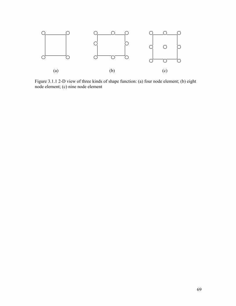
69

(a) (b) (c)

Figure 3.1.1 2-D view of three kinds of shape function: (a) four node element; (b) eight node element; (c) nine node element

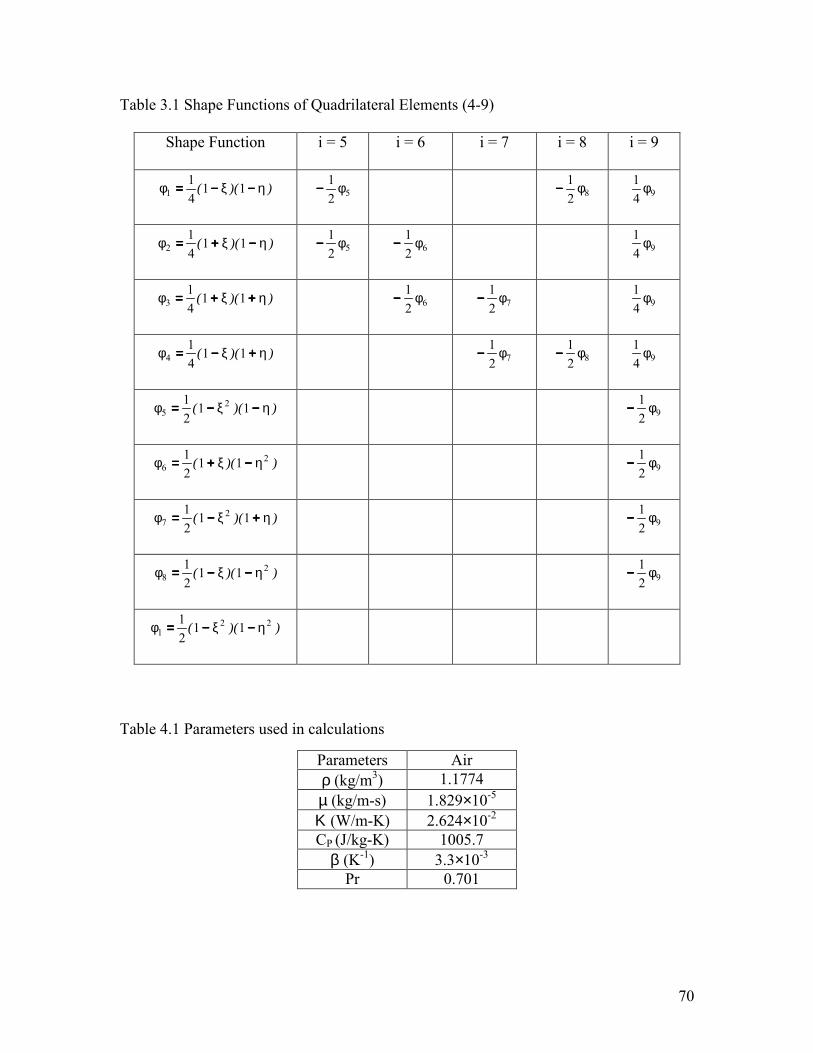
70

Table 3.1 Shape Functions of Quadrilateral Elements (4-9)

Shape Function i = 5 i = 6 i = 7 i = 8 i = 9

))(( ηξφ −−−−−−−−==== 1141

1 521 φ−−−− 82

1 φ−−−− 941 φ

))(( ηξφ −−−−++++==== 1141

2 521 φ−−−− 62

1 φ−−−− 941 φ

))(( ηξφ ++++++++==== 1141

3 621 φ−−−− 72

1 φ−−−− 941 φ

))(( ηξφ ++++−−−−==== 1141

4 721 φ−−−− 82

1 φ−−−− 941 φ

))(( ηξφ −−−−−−−−==== 1121 2

5 921 φ−−−−

))(( 26 11

21 ηξφ −−−−++++==== 92

1 φ−−−−

))(( ηξφ ++++−−−−==== 1121 2

7 921 φ−−−−

))(( 28 11

21 ηξφ −−−−−−−−==== 92

1 φ−−−−

))(( 221 11

21 ηξφ −−−−−−−−====

Table 4.1 Parameters used in calculations

Parameters Air ρ (kg/m3) 1.1774 µ (kg/m-s) 1.829×10-5

Κ (W/m-K) 2.624×10-2

CP (J/kg-K) 1005.7 β (K-1) 3.3×10-3

Pr 0.701

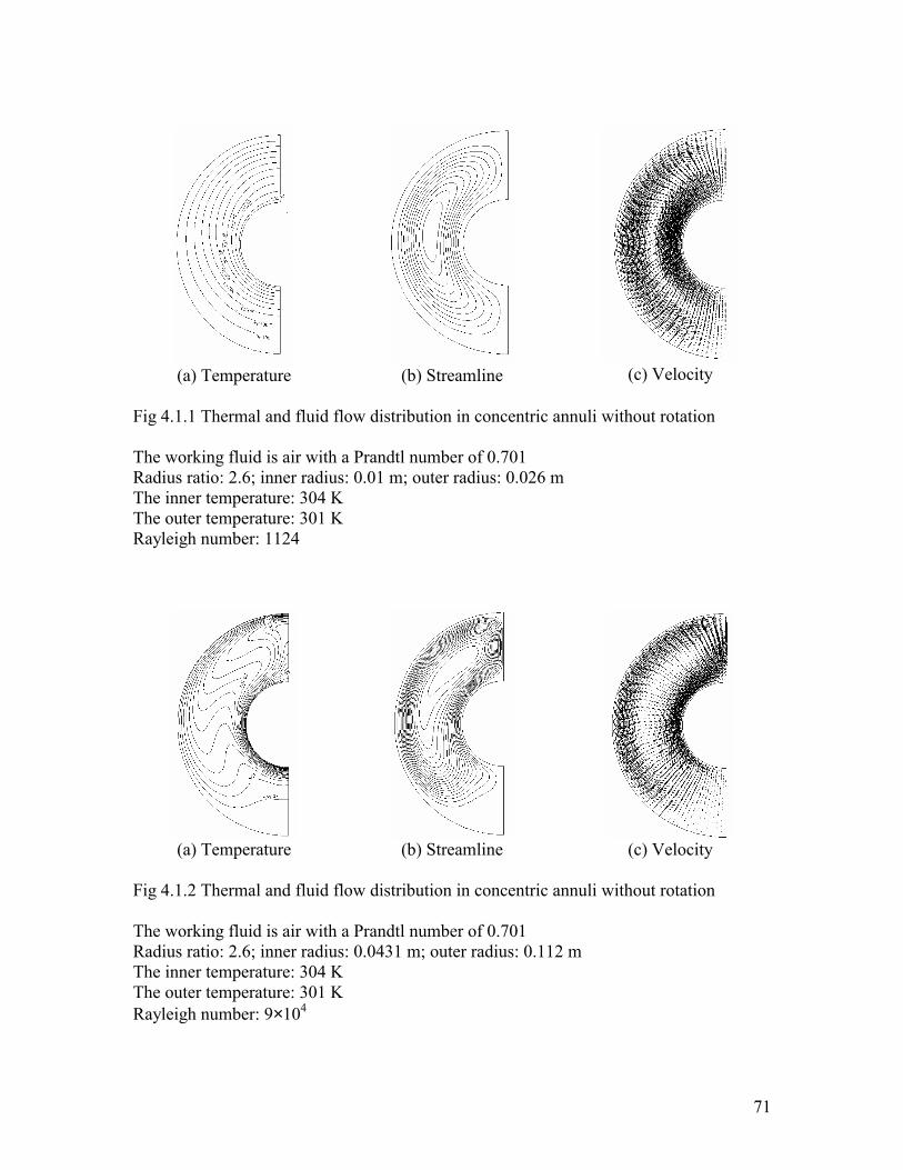
71

(a) Temperature

(b) Streamline

(c) Velocity

Fig 4.1.1 Thermal and fluid flow distribution in concentric annuli without rotation The working fluid is air with a Prandtl number of 0.701 Radius ratio: 2.6; inner radius: 0.01 m; outer radius: 0.026 m The inner temperature: 304 K The outer temperature: 301 K Rayleigh number: 1124

(a) Temperature

(b) Streamline

(c) Velocity

Fig 4.1.2 Thermal and fluid flow distribution in concentric annuli without rotation The working fluid is air with a Prandtl number of 0.701 Radius ratio: 2.6; inner radius: 0.0431 m; outer radius: 0.112 m The inner temperature: 304 K The outer temperature: 301 K Rayleigh number: 9×104

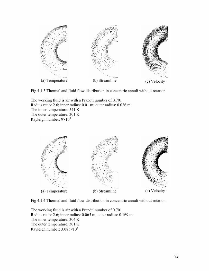
72

(a) Temperature

(b) Streamline

(c) Velocity

Fig 4.1.3 Thermal and fluid flow distribution in concentric annuli without rotation The working fluid is air with a Prandtl number of 0.701 Radius ratio: 2.6; inner radius: 0.01 m; outer radius: 0.026 m The inner temperature: 541 K The outer temperature: 301 K Rayleigh number: 9×104

(a) Temperature

(b) Streamline

(c) Velocity

Fig 4.1.4 Thermal and fluid flow distribution in concentric annuli without rotation The working fluid is air with a Prandtl number of 0.701 Radius ratio: 2.6; inner radius: 0.065 m; outer radius: 0.169 m The inner temperature: 304 K The outer temperature: 301 K Rayleigh number: 3.085×105

73

(a) Temperature

(b) Streamline

(c) Velocity

Fig 4.1.5 Thermal and fluid flow distribution in concentric annuli without rotation The working fluid is air with a Prandtl number of 0.701 Radius ratio: 2.6; inner radius: 0.07 m; outer radius: 0.182 m The inner temperature: 304 K The outer temperature: 301 K Rayleigh number: 3.85×105

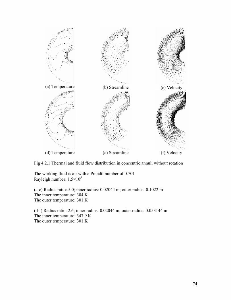
74

(a) Temperature

(b) Streamline

(c) Velocity

(d) Temperature

(e) Streamline

(f) Velocity

Fig 4.2.1 Thermal and fluid flow distribution in concentric annuli without rotation The working fluid is air with a Prandtl number of 0.701 Rayleigh number: 1.5×105

(a-c) Radius ratio: 5.0; inner radius: 0.02044 m; outer radius: 0.1022 m The inner temperature: 304 K The outer temperature: 301 K (d-f) Radius ratio: 2.6; inner radius: 0.02044 m; outer radius: 0.053144 m The inner temperature: 347.9 K The outer temperature: 301 K

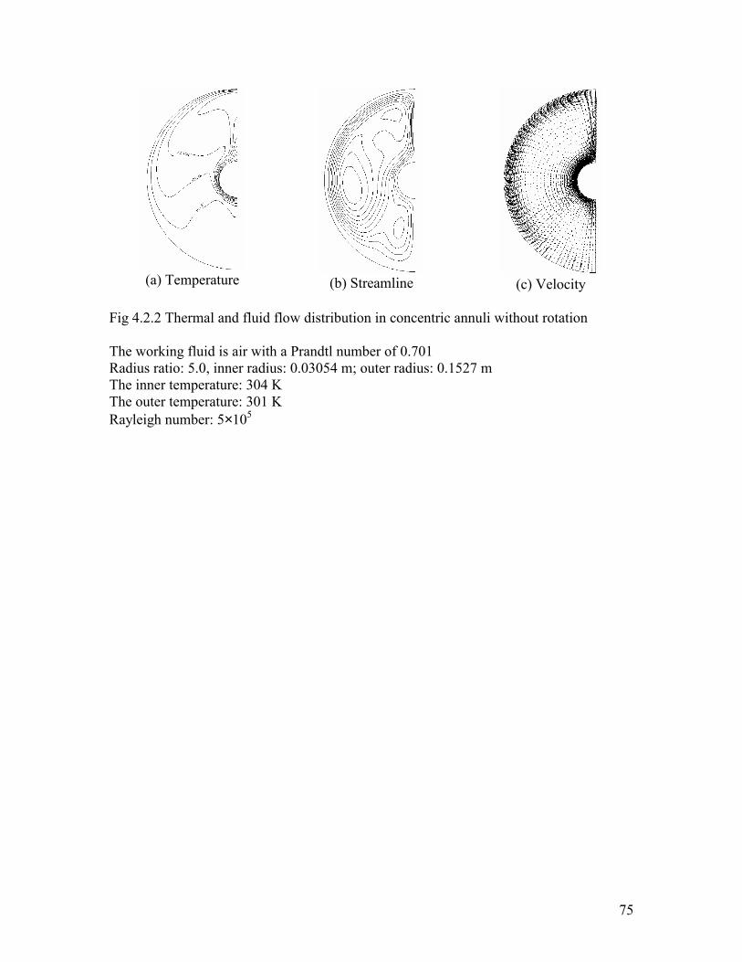
75

(a) Temperature

(b) Streamline

(c) Velocity

Fig 4.2.2 Thermal and fluid flow distribution in concentric annuli without rotation The working fluid is air with a Prandtl number of 0.701 Radius ratio: 5.0, inner radius: 0.03054 m; outer radius: 0.1527 m The inner temperature: 304 K The outer temperature: 301 K Rayleigh number: 5×105

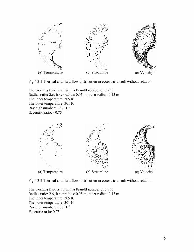
76

(a) Temperature

(b) Streamline

(c) Velocity

Fig 4.3.1 Thermal and fluid flow distribution in eccentric annuli without rotation The working fluid is air with a Prandtl number of 0.701 Radius ratio: 2.6, inner radius: 0.05 m; outer radius: 0.13 m The inner temperature: 305 K The outer temperature: 301 K Rayleigh number: 1.87×105

Eccentric ratio: - 0.75

(a) Temperature

(b) Streamline

(c) Velocity

Fig 4.3.2 Thermal and fluid flow distribution in eccentric annuli without rotation The working fluid is air with a Prandtl number of 0.701 Radius ratio: 2.6, inner radius: 0.05 m; outer radius: 0.13 m The inner temperature: 305 K The outer temperature: 301 K Rayleigh number: 1.87×105 Eccentric ratio: 0.75

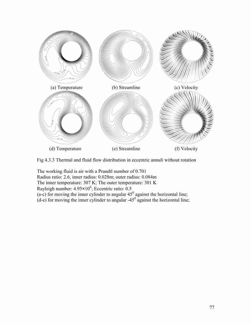
77

(a) Temperature (b) Streamline (c) Velocity

(d) Temperature (e) Streamline (f) Velocity

Fig 4.3.3 Thermal and fluid flow distribution in eccentric annuli without rotation The working fluid is air with a Prandtl number of 0.701 Radius ratio: 2.6, inner radius: 0.028m; outer radius: 0.084m The inner temperature: 307 K; The outer temperature: 301 K Rayleigh number: 4.95×104; Eccentric ratio: 0.5 (a-c) for moving the inner cylinder to angular 450 against the horizontal line; (d-e) for moving the inner cylinder to angular -450 against the horizontal line;

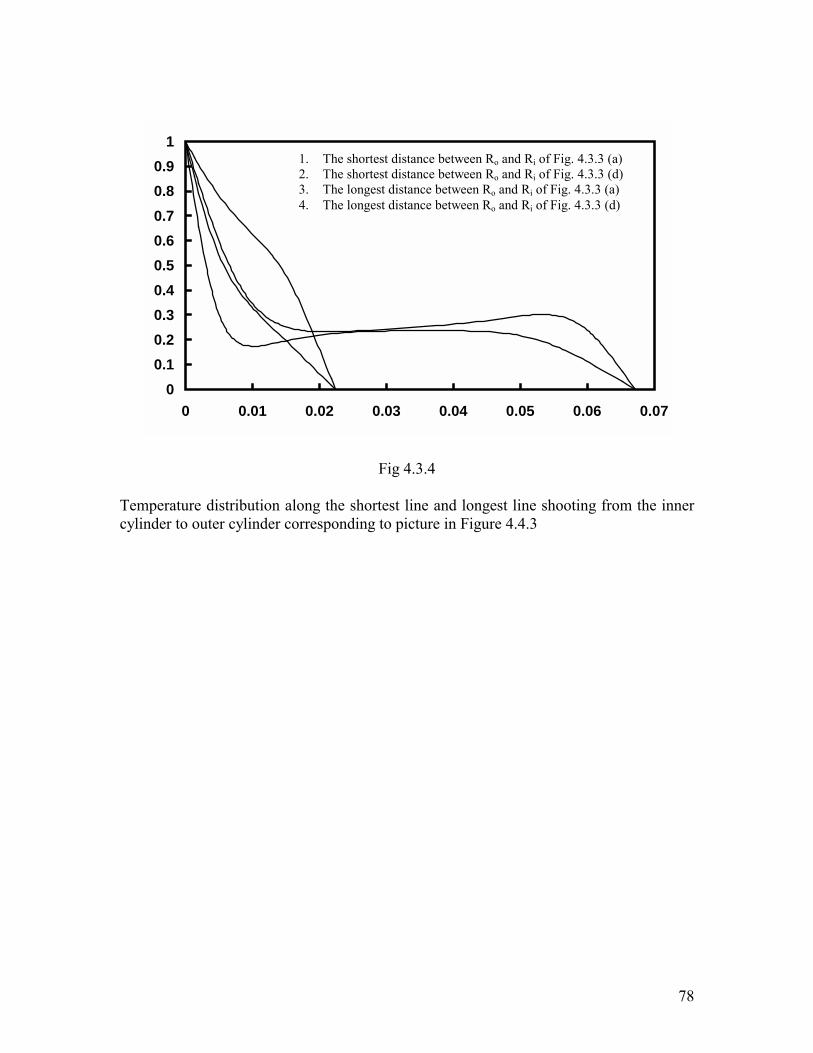
78

00.10.20.30.40.50.60.70.80.9

1

0 0.01 0.02 0.03 0.04 0.05 0.06 0.07

Fig 4.3.4

Temperature distribution along the shortest line and longest line shooting from the inner cylinder to outer cylinder corresponding to picture in Figure 4.4.3

1. The shortest distance between Ro and Ri of Fig. 4.3.3 (a) 2. The shortest distance between Ro and Ri of Fig. 4.3.3 (d) 3. The longest distance between Ro and Ri of Fig. 4.3.3 (a) 4. The longest distance between Ro and Ri of Fig. 4.3.3 (d)

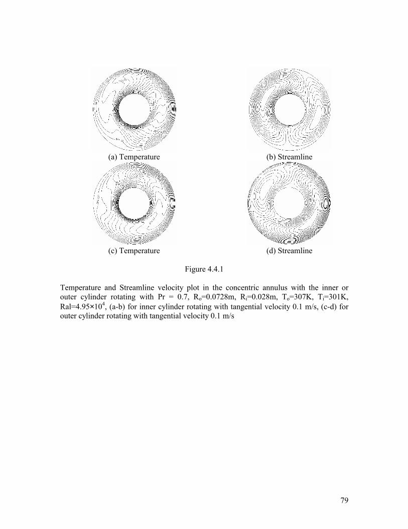
79

(a) Temperature (b) Streamline

(c) Temperature (d) Streamline

Figure 4.4.1

Temperature and Streamline velocity plot in the concentric annulus with the inner or outer cylinder rotating with Pr = 0.7, Ro=0.0728m, Ri=0.028m, To=307K, Ti=301K, Ral=4.95×104, (a-b) for inner cylinder rotating with tangential velocity 0.1 m/s, (c-d) for outer cylinder rotating with tangential velocity 0.1 m/s

80

0

0.1

0.2

0.3

0.4

0.5

0.6

0.7

0.8

0.9

1

0 0.01 0.02 0.03 0.04 0.05

Figure 4.4.2

Temperature distribution along different angular line shooting from the inner cylinder to outer cylinder corresponding to picture in Figure 4.4.1.

1

2

3

4

56

7

8

1. 00 (Vo= 0.1) 2. 900 (Vo= 0.1) 3. 1800 (Vo= 0.1) 4. 2700 (Vo= 0.1) 5. 00 (Vi = 0.1) 6. 900 (Vi= 0.1) 7. 1800 (Vi= 0.1) 8. 2700 (Vi= 0.1)

Distance from Ro to Ri (m)

(T-T

o)/(T

i-To)

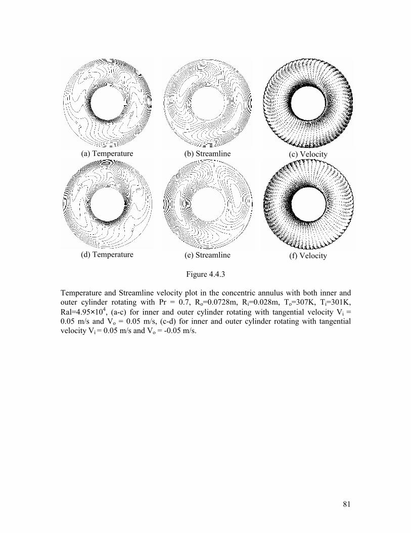
81

(a) Temperature

(b) Streamline

(c) Velocity

(d) Temperature (e) Streamline (f) Velocity

Figure 4.4.3

Temperature and Streamline velocity plot in the concentric annulus with both inner and outer cylinder rotating with Pr = 0.7, Ro=0.0728m, Ri=0.028m, To=307K, Ti=301K, Ral=4.95×104, (a-c) for inner and outer cylinder rotating with tangential velocity Vi = 0.05 m/s and Vo = 0.05 m/s, (c-d) for inner and outer cylinder rotating with tangential velocity Vi = 0.05 m/s and Vo = -0.05 m/s.

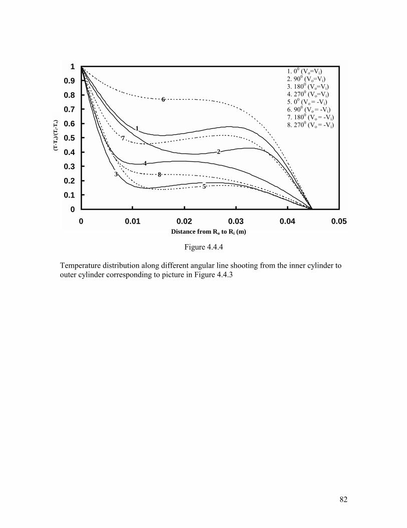
82

0

0.1

0.2

0.3

0.4

0.5

0.6

0.7

0.8

0.9

1

0 0.01 0.02 0.03 0.04 0.05

Figure 4.4.4

Temperature distribution along different angular line shooting from the inner cylinder to outer cylinder corresponding to picture in Figure 4.4.3

1

2

34

5

6

7

8

Distance from Ro to Ri (m)

(T-T

o)/(T

i-To)

1. 00 (Vo=Vi) 2. 900 (Vo=Vi) 3. 1800 (Vo=Vi) 4. 2700 (Vo=Vi) 5. 00 (Vo = -Vi) 6. 900 (Vo = -Vi) 7. 1800 (Vo = -Vi) 8. 2700 (Vo = -Vi)

83

(a) Temperature

(b) Streamline

(c) Velocity

(d) Temperature

(e) Streamline

(f) Velocity

Figure 4.5.1

Temperature and Streamline velocity plot in the eccentric annulus of inner cylinder moving up with both inner and outer cylinder rotating with Pr = 0.7, Ro=0.0728m, Ri=0.028m, To=307K, Ti=301K, Ral=4.95×104 and er=0.5, (a-c) for inner and outer cylinder rotating with tangential velocity Vi = 0.05 m/s and Vo = 0.05 m/s, (c-d) for inner and outer cylinder rotating with tangential velocity Vi = 0.05 m/s and Vo = -0.05 m/s.

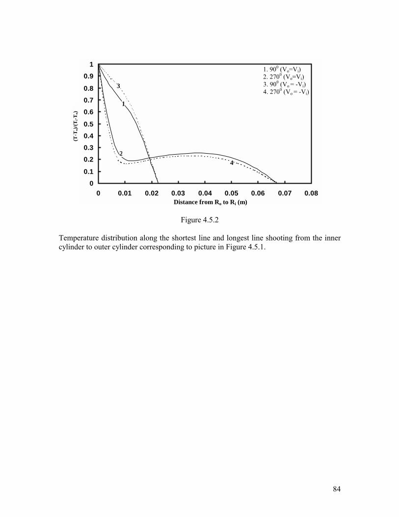
84

00.1

0.20.30.40.5

0.60.70.8

0.91

0 0.01 0.02 0.03 0.04 0.05 0.06 0.07 0.08

Figure 4.5.2

Temperature distribution along the shortest line and longest line shooting from the inner cylinder to outer cylinder corresponding to picture in Figure 4.5.1.

1

2

3

4

Distance from Ro to Ri (m)

(T-T

o)/(T

i-To)

1. 900 (Vo=Vi) 2. 2700 (Vo=Vi) 3. 900 (Vo = -Vi) 4. 2700 (Vo = -Vi)

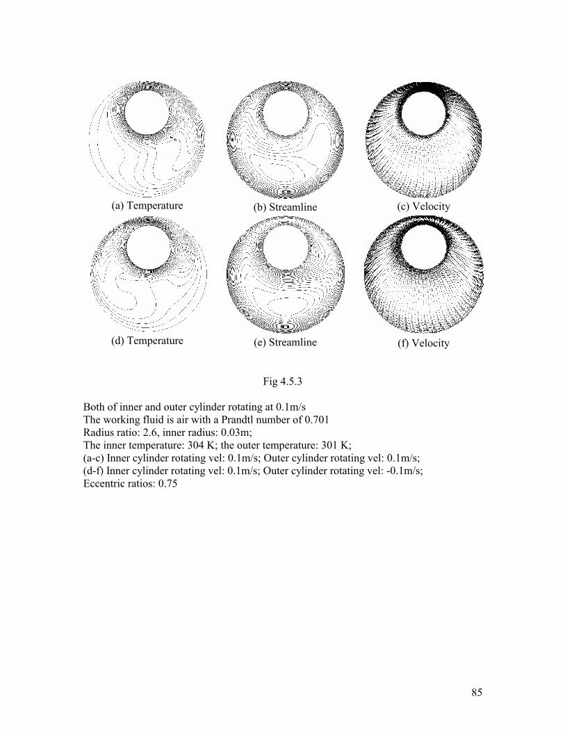
85

(a) Temperature

(b) Streamline

(c) Velocity

(d) Temperature

(e) Streamline

(f) Velocity

Fig 4.5.3

Both of inner and outer cylinder rotating at 0.1m/s The working fluid is air with a Prandtl number of 0.701 Radius ratio: 2.6, inner radius: 0.03m; The inner temperature: 304 K; the outer temperature: 301 K; (a-c) Inner cylinder rotating vel: 0.1m/s; Outer cylinder rotating vel: 0.1m/s; (d-f) Inner cylinder rotating vel: 0.1m/s; Outer cylinder rotating vel: -0.1m/s; Eccentric ratios: 0.75

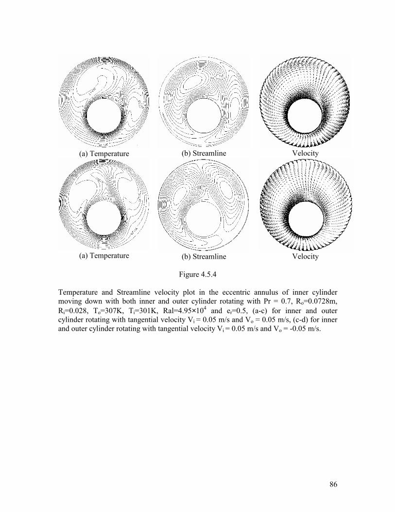
86

(a) Temperature (b) Streamline

Velocity

(a) Temperature

(b) Streamline Velocity

Figure 4.5.4

Temperature and Streamline velocity plot in the eccentric annulus of inner cylinder moving down with both inner and outer cylinder rotating with Pr = 0.7, Ro=0.0728m, Ri=0.028, To=307K, Ti=301K, Ral=4.95×104 and er=0.5, (a-c) for inner and outer cylinder rotating with tangential velocity Vi = 0.05 m/s and Vo = 0.05 m/s, (c-d) for inner and outer cylinder rotating with tangential velocity Vi = 0.05 m/s and Vo = -0.05 m/s.

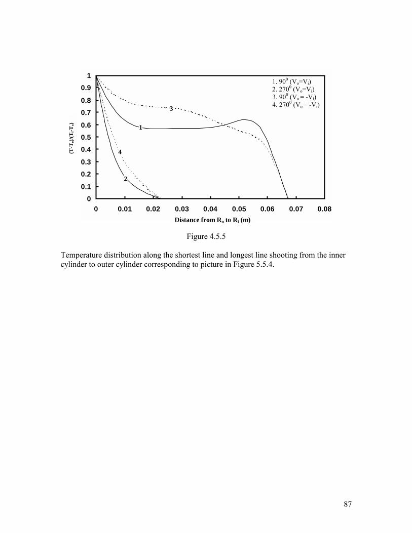
87

00.1

0.20.3

0.40.50.6

0.70.8

0.91

0 0.01 0.02 0.03 0.04 0.05 0.06 0.07 0.08

Figure 4.5.5

Temperature distribution along the shortest line and longest line shooting from the inner cylinder to outer cylinder corresponding to picture in Figure 5.5.4.

1

2

3

4

1. 900 (Vo=Vi) 2. 2700 (Vo=Vi) 3. 900 (Vo = -Vi) 4. 2700 (Vo = -Vi)

Distance from Ro to Ri (m)

(T-T

o)/(T

i-To)

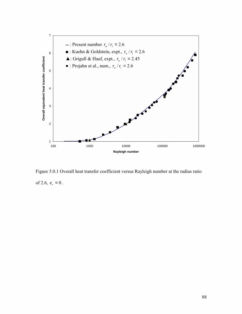
88

1

2

3

4

5

6

7

100 1000 10000 100000 1000000

Rayleigh number

Ove

rall

equi

vale

nt h

eat t

rans

fer c

oeffi

cien

t

Figure 5.0.1 Overall heat transfer coefficient versus Rayleigh number at the radius ratio

of 2.6, 0=re .

: Present number 6.2/ =io rr : Kuehn & Goldstein, expt., 6.2/ =io rr : Grigull & Hauf, expt., 45.2/ =io rr : Projahn et al., num., 6.2/ =io rr

89

(a) 2102×=Ral (b) 310=Ral

(c) 410=Ral (d) 4105×=Ral

(e) 510=Ral (f) 610=Ral

Fig. 5.1.1 Isotherm plots at various Rayleigh number, ,6.2/ =io rr .0=re

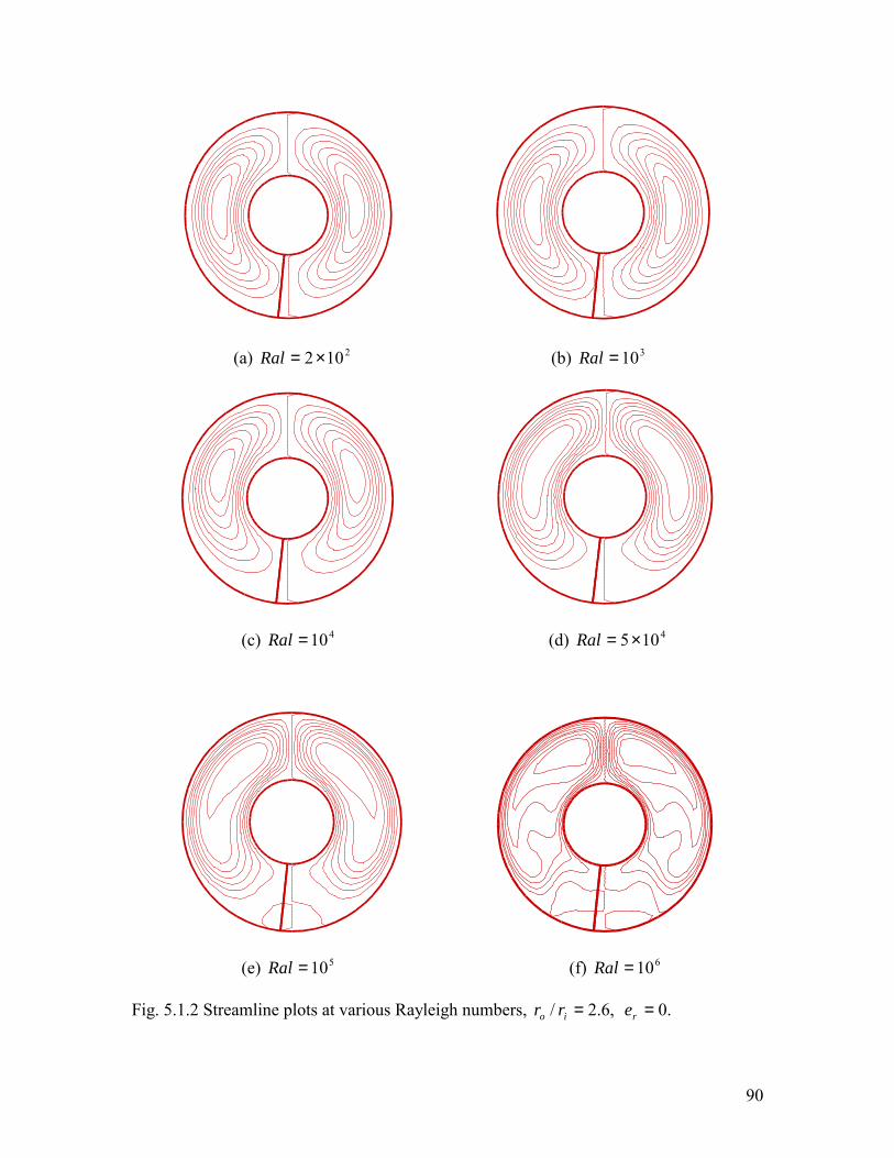
90

(a) 2102×=Ral (b) 310=Ral

(c) 410=Ral (d) 4105×=Ral

(e) 510=Ral (f) 610=Ral

Fig. 5.1.2 Streamline plots at various Rayleigh numbers, ,6.2/ =io rr .0=re

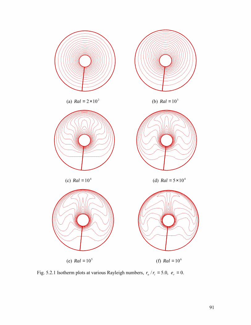
91

(a) 2102×=Ral (b) 310=Ral

(c) 410=Ral (d) 4105×=Ral

(e) 510=Ral (f) 610=Ral

Fig. 5.2.1 Isotherm plots at various Rayleigh numbers, ,0.5/ =io rr .0=re

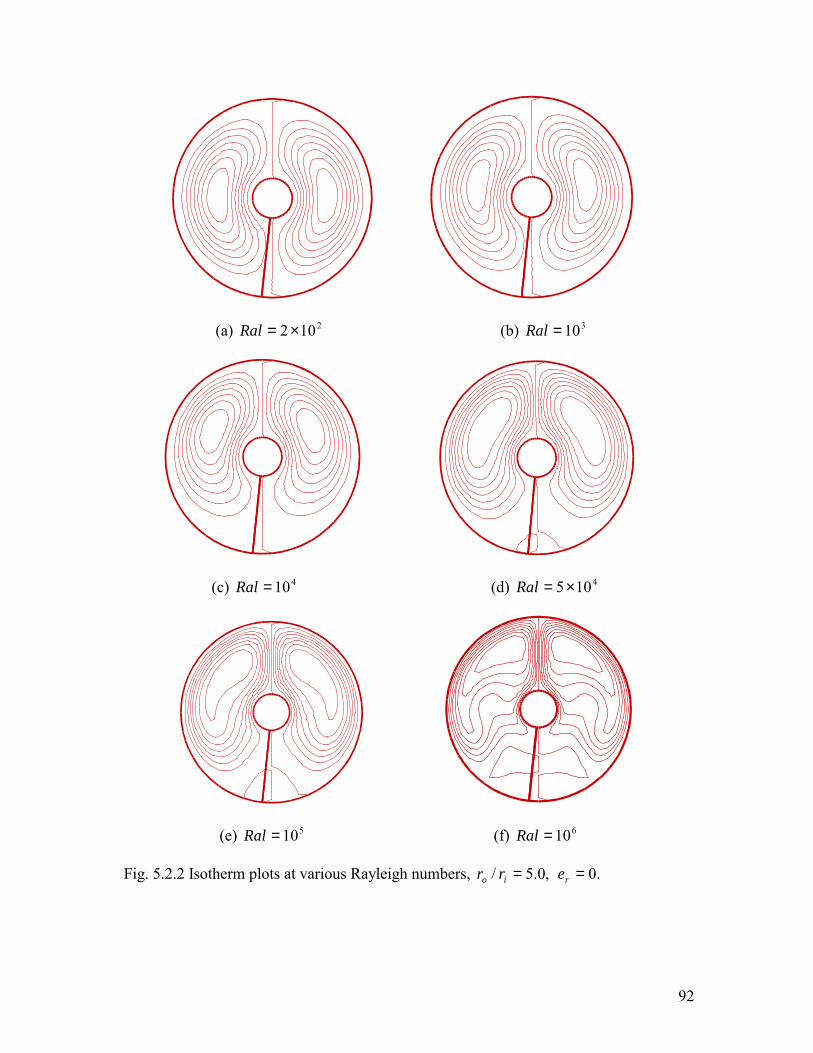
92

(a) 2102×=Ral (b) 310=Ral

(c) 410=Ral (d) 4105×=Ral

(e) 510=Ral (f) 610=Ral

Fig. 5.2.2 Isotherm plots at various Rayleigh numbers, ,0.5/ =io rr .0=re

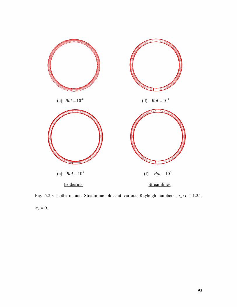
93

(c) 410=Ral (d) 410=Ral

(e) 510=Ral (f) 510=Ral

Isotherms Streamlines

Fig. 5.2.3 Isotherm and Streamline plots at various Rayleigh numbers, ,25.1/ =io rr

.0=re

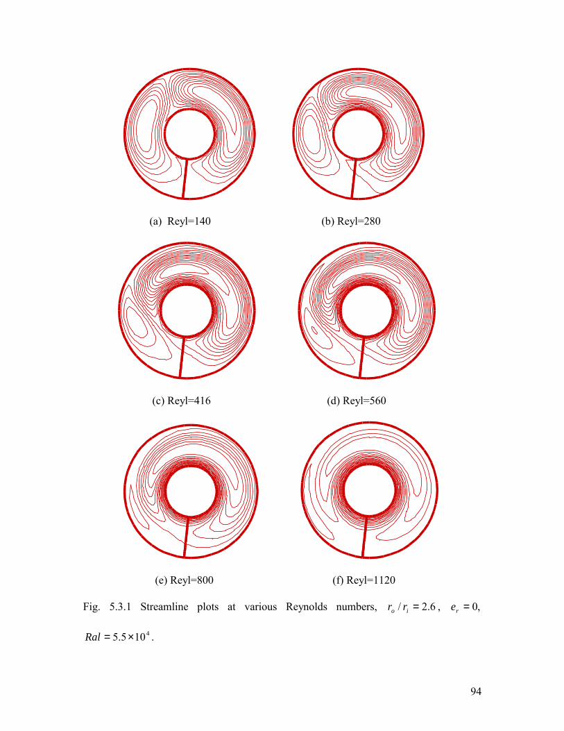
94

(a) Reyl=140 (b) Reyl=280

(c) Reyl=416 (d) Reyl=560

(e) Reyl=800 (f) Reyl=1120

Fig. 5.3.1 Streamline plots at various Reynolds numbers, 6.2/ =io rr , ,0=re

4105.5 ×=Ral .

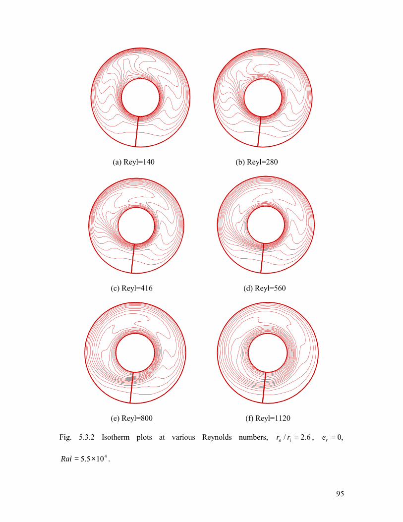
95

(a) Reyl=140 (b) Reyl=280

(c) Reyl=416 (d) Reyl=560

(e) Reyl=800 (f) Reyl=1120

Fig. 5.3.2 Isotherm plots at various Reynolds numbers, 6.2/ =io rr , ,0=re

4105.5 ×=Ral .

96

(a) )31,0(=

− re (b) )

31,0(=

− re

(c) )31,0( −=

− re (d) )

31,0( −=

− re

(e) )0,31(−=

− re (f) )0,

31(−=

− re

Fig. 5.4.1 Isotherm and streamline plots at various eccentric positions, ,6.2/0 =irr

,31=e 4105×=Ral .

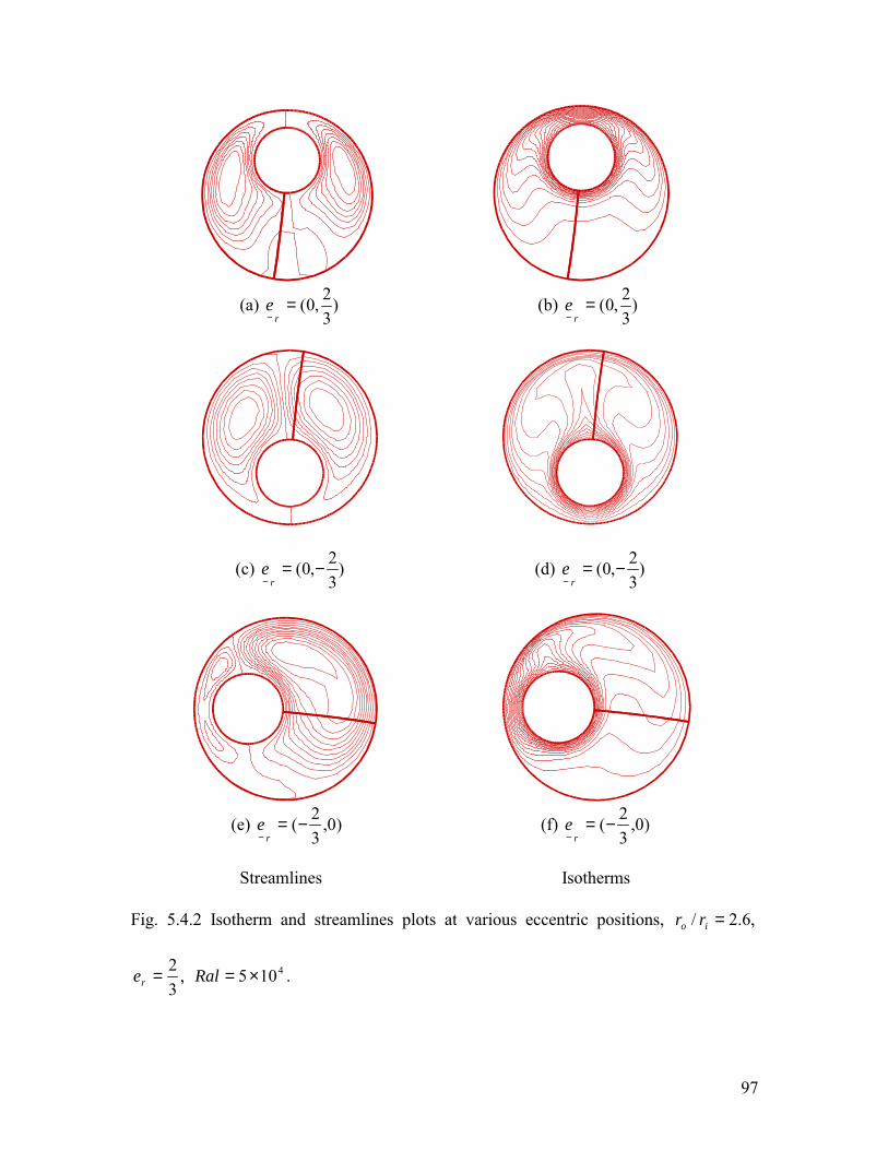
97

(a) )

32,0(=

− re (b) )

32,0(=

− re

(c) )32,0( −=

− re (d) )

32,0( −=

− re

(e) )0,

32(−=

− re (f) )0,

32(−=

− re

Streamlines Isotherms

Fig. 5.4.2 Isotherm and streamlines plots at various eccentric positions, ,6.2/ =io rr

,32=re 4105×=Ral .

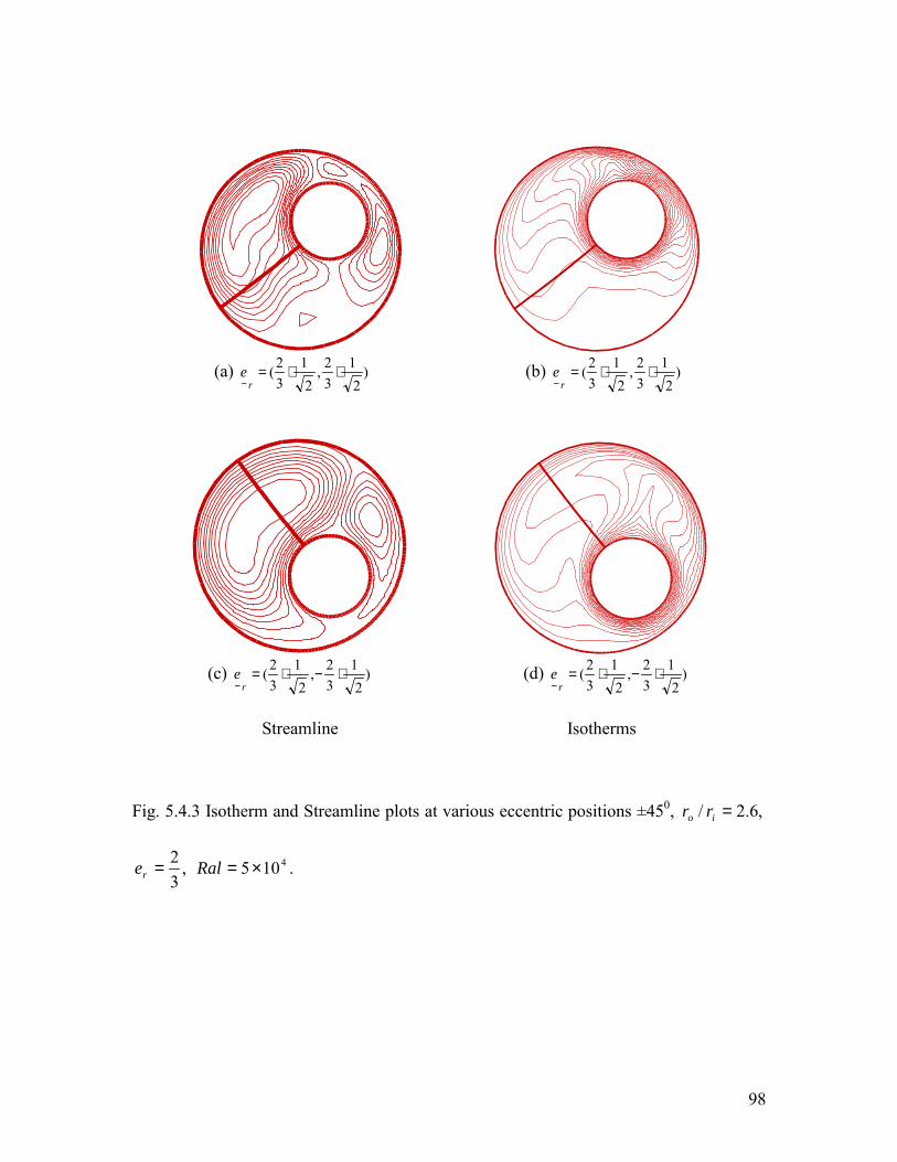
98

(a) )

21

32,

21

32( ⋅⋅=

− re (b) )

21

32,

21

32( ⋅⋅=

− re

(c) )

21

32,

21

32( ⋅−⋅=

− re (d) )

21

32,

21

32( ⋅−⋅=

− re

Streamline Isotherms

Fig. 5.4.3 Isotherm and Streamline plots at various eccentric positions ±450, ,6.2/ =io rr

,32=re 4105×=Ral .

99

(a) )31,0(=

− re (b) )

31,0( −=

− re

(c) )0,31(−=

− re (d) )0,

31(=

− re

Fig. 5.5.1 Streamline plots at eccentric positions, ,6.2/ =io rr ,31=re ,105.5 4×=Ral

Rey1=280.

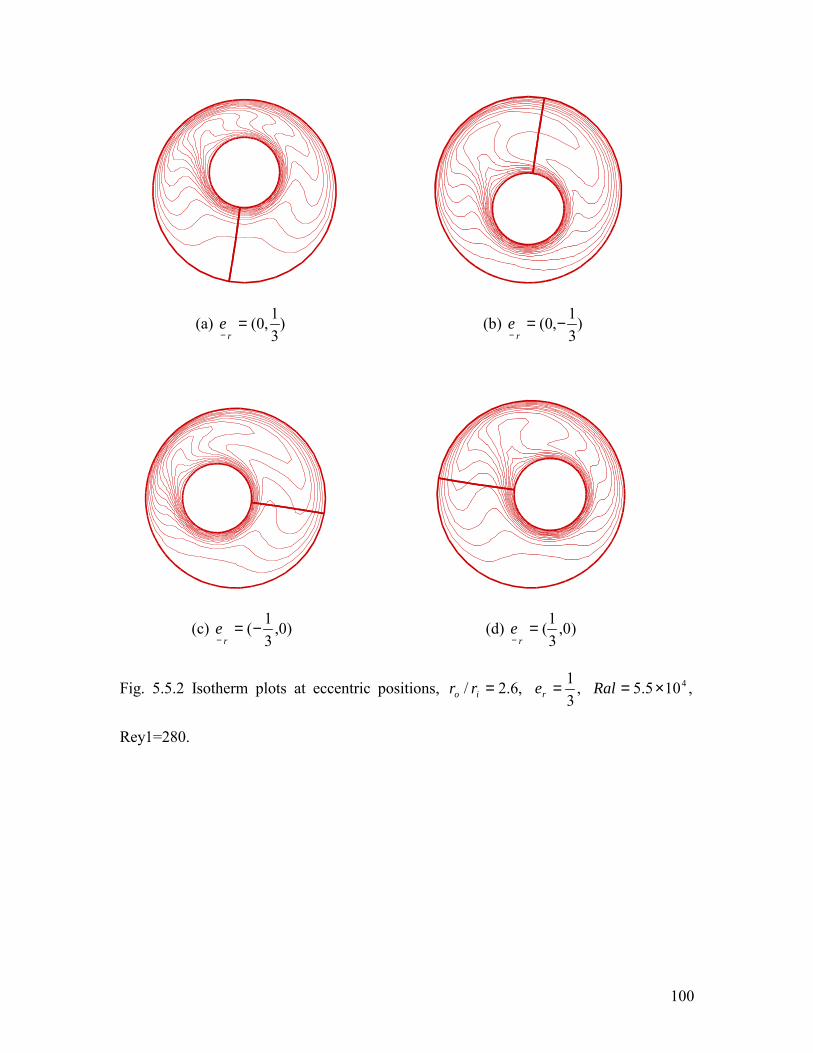
100

(a) )31,0(=

− re (b) )

31,0( −=

− re

(c) )0,31(−=

− re (d) )0,

31(=

− re

Fig. 5.5.2 Isotherm plots at eccentric positions, ,6.2/ =io rr ,31=re ,105.5 4×=Ral

Rey1=280.

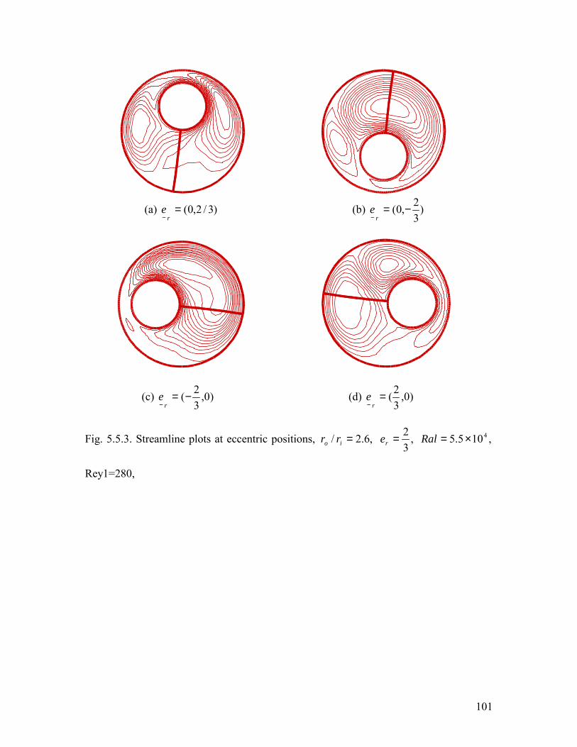
101

(a) )3/2,0(=

− re (b) )

32,0( −=

− re

(c) )0,32(−=

− re (d) )0,

32(=

− re

Fig. 5.5.3. Streamline plots at eccentric positions, ,6.2/ =io rr ,32=re ,105.5 4×=Ral

Rey1=280,

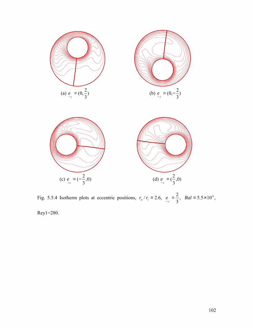
102

(a) )

32,0(=

− re (b) )

32,0( −=

− re

(c) )0,

32(−=

− re (d) )0,

32(=

− re

Fig. 5.5.4 Isotherm plots at eccentric positions, ,6.2/ =io rr ,32=

− re ,105.5 4×=Ral

Rey1=280.

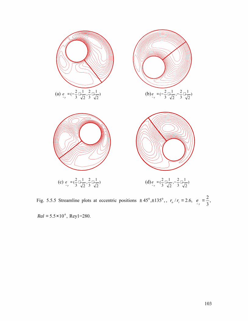
103

(a) )

21

32,

21

32( ⋅⋅−=

− re (b) )

21

32,

21

32( ⋅−⋅−=

− re

(c) )2

132,

21

32( ⋅⋅=

− re (d) )

21

32,

21

32( ⋅−⋅=

− re

Fig. 5.5.5 Streamline plots at eccentric positions ,135,45 00 ±± , ,6.2/ =io rr ,32=

− re

,105.5 4×=Ral Rey1=280.

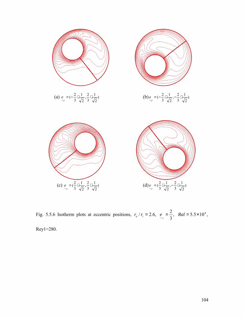
104

(a) )2

132,

21

32( ⋅⋅−=

− re (b) )

21

32,

21

32( ⋅−⋅−=

− re

(c) )

21

32,

21

32( ⋅⋅=

− re (d) )

21

32,

21

32( ⋅−⋅=

− re

Fig. 5.5.6 Isotherm plots at eccentric positions, ,6.2/ =io rr ,32=

− re ,105.5 4×=Ral

Rey1=280.