applied sciences

Article

Numerical Study on the Asphalt Concrete Structurefor Blast and Impact Load Using the Karagozian andCase Concrete Model

Jun Wu 1,2, Liang Li 1,*, Xiuli Du 1 and Xuemei Liu 3

1 The Key Laboratory of Urban Security and Disaster Engineering, Ministry of Education,Beijing University of Technology, Beijing 100124, China; cvewujun@sues.edu.cn (J.W.);duxiuli@bjut.edu.cn (X.D.)

2 School of Urban Railway Transportation, Shanghai University of Engineering Science,Shanghai 201620, China

3 School of Civil Engineering and Built Environment, Queensland University of Technology,Brisbane 4001, Australia; x51.liu@qut.edu.au

* Correspondence: liliang@bjut.edu.cn; Tel.: +86-10-6739-2430

Academic Editor: Zhanping YouReceived: 23 November 2016; Accepted: 14 February 2017; Published: 17 February 2017

Abstract: The behaviour of an asphalt concrete structure subjected to severe loading, such as blastand impact loadings, is becoming critical for safety and anti-terrorist reasons. With the developmentof high-speed computational capabilities, it is possible to carry out the numerical simulation ofan asphalt concrete structure subjected to blast or impact loading. In the simulation, the constitutivemodel plays a key role as the model defines the essential physical mechanisms of the material underdifferent stress and loading conditions. In this paper, the key features of the Karagozian and Caseconcrete model (KCC) adopted in LSDYNA are evaluated and discussed. The formulations of thestrength surfaces and the damage factor in the KCC model are verified. Both static and dynamictests are used to determine the parameters of asphalt concrete in the KCC model. The modifieddamage factor is proposed to represent the higher failure strain that can improve the simulation ofthe behaviour of AC material. Furthermore, a series test of the asphalt concrete structure subjectedto blast and impact loadings is conducted and simulated by using the KCC model. The simulationresults are then compared with those from both field and laboratory tests. The results show that theuse of the KCC model to simulate asphalt concrete structures can reproduce similar results as thefield and laboratory test.

Keywords: asphalt concrete; constitutive model; impact loading; blast loading; numerical simulation

1. Introduction

The behaviour of structures or infrastructures under extreme loadings has become a hot topicin the area of civil, mechanical and material engineering. Critical infrastructures, such as runwaypavement designed for normal aircraft landing and taking off, are expected to have adequate resistancewhen subjected to extreme loadings, such as impact or blast loadings (e.g., heavy airplane landingor taking off, air plane crash or terrorist attack). Asphalt concrete (AC) is made of bitumen binderand coarse aggregate. It is usually used as the surface course for both highway and runway flexiblepavement [1]. The dynamic load in the daily application for AC pavement normally correspondsto a strain rate less than 10−1 s−1. Tashman et al. [2] conducted experiments of AC under triaxialcompressive loading at the strain rate from 10−6 s−1 to 10−3 s−1. The results showed that the failurestress increased with the increase of the applied strain rate. Seibi et al. [3] studied AC subjected touniaxial compressive loading with strain rate from 0.064 s−1 to 0.28 s−1. It was found that the yield

Appl. Sci. 2017, 7, 202; doi:10.3390/app7020202 www.mdpi.com/journal/applsci

Appl. Sci. 2017, 7, 202 2 of 22

stress was significantly dependent on the strain rate. Park et al. [4] carried out tests on AC underuniaxial and triaxial compression with the strain rate changing from 10−4 s−1 to 0.07 s−1. The resultsshowed that with the increase of the applied strain rates, the yield stress and failure stress increased,and the strain rate dependency was clearly showing up at the higher strains. It was also found that theviscous behaviour of AC decreased with the increase of the strain rate. However, when the pavementstructure is subjected to the impact loading from further heavy traffic loading or aircraft loading, thecorresponding strain rate exceeds 10−1 s−1, especially for heavy aircraft loading, the related strain ratereaches around 100 s−1. Based on previous research [5,6], the compressive strength of AC material canbe enhanced with the increase of strain rate, and AC material exhibits high plastic behaviour at thehigh strain rate. However, it is very expensive to conduct field test to investigate the actual behaviourof AC under severe dynamic loading, the numerical simulation is an effective alternative solution.

There are many factors that influence the reliability of numerical simulation. Among these factors,the material model plays a key role because it should reproduce the essential physical mechanisms ofthe material under various loading conditions. Seibi et al. [3] and Park et al. [4] used the Drucker–Prageryield function to simulate the compressive behaviour of AC under dynamic strain loading (strainrate from 0.0001 s−1 to 0.0701 s−1). Tashman et al. [2] developed a microstructure-based viscoplasticcontinuum model to take into account the effect of temperature in AC material with the strain rateranging from 10−6 s−1 to 10−3 s−1. Since the late 1990s, microstructural-based discrete element models(DEM) have been used for better understanding of asphalt pavement concrete (e.g., [7–10]). In DEMmodels, the assumption of elastic or viscoelastic behaviour was employed for the simulation of thestatic or creep behaviour of AC under normal traffic loading. However, it was found that when thepavement structure was under blast or high impact load, plastic deformation and severe damage wouldoccur. Thus, a robust material model should be developed to consider the strain rate effect, strainhardening, strain softening and damage of the AC material under the severe dynamic loading. Recently,several concrete-like material models subjected to dynamic loadings have been developed, such as theRiedel-Hiermaier-Thoma (RHT) model [11], the Advanced Fundamental Concrete (AFC) model [12,13],the Karagozian and Case concrete model (KCC) [14] and the Holmquist-Johnson-Cook (HJC) concretemodel [15,16]. These robust material models are capable of capturing varying concrete-like materials’behaviour under different loading conditions. When subjected to dynamic loading, such as blastloading or high impact loading, concrete-like materials show a highly non-linear response. Besides,due to the general complexity of the constitutive models, the determination of the parameters (i.e.,residual strength, failure strain and failure criteria in model) also plays an important role in achievingthe actual performance of the concrete-like materials. This requires sufficient understanding of themodelling formulation and the associated considerations. In the current study, the KCC model [14] isused to simulate the AC material. This model is capable of capturing the varied concrete-like materialbehaviours under different loading conditions. However, it should be noticed that this model cannotconsider the temperature effect. In this study, the dynamic behaviour of AC under a high strain rate isinvestigated, and the temperature effect is not considered. Hence, the KCC can be used; otherwise, thetemperature issue should come up.

In this paper, several key features of the KCC model are firstly discussed, and then, thedetermination of the parameters in the KCC model for AC is provided. An application exampleon the AC structure under blast and impact loading is also illustrated and validated based on a fieldblast test and a laboratory drop weight impact test.

2. Review on KCC Model

When subjected to blast loading or high impact loading, concrete or other concrete-like materialsshows a highly non-linear response. They usually exhibit pressure hardening and strain hardeningunder static loading and strain rate hardening in tension and compression under dynamic loading.A number of material models has been developed to model concrete-like materials recently [11–16].Among them, the KCC model is widely used to analyse concrete-like materials’ response to blast

Appl. Sci. 2017, 7, 202 3 of 22

and impact loading due to its simple implementation. In addition, the KCC model can capture thenon-linear behaviour of the material under dynamic loading [14]. The key features of the model arediscussed briefly in the following section.

2.1. Strength Surface in KCC Model

The KCC model decouples stress into the hydrostatic pressure and deviatoric stress as shown inEquation (1):

σij = sij +13

σiiδij (1)

where σij is the stress tensor, sij is the deviatoric stress tensor and σii is the hydrostatic pressuretensor. It should be noted that stress is positive in tension, and pressure is positive in compression.The hydrostatic pressure is related to the volumetric change of material, while the deviatoric stressis related to shear resistance of the material and is usually expressed by the second invariant of thedeviatoric stress tensor, J2:

J2 =12

sijsji =s2

1 + s22 + s2

32

(2)

The KCC model has three independent strength surfaces: maximum strength surface, yieldsurface and residual strength surface, which are shown in Figure 1. The general formation of strengthsurfaces can be written as:

∆σ =√

3J2 = f (p, J2) (3)

in which ∆σ is the principal stress difference and p is the hydrostatic pressure. Usually, the aboveEquation (3) refers to the compressive meridian. The whole failure curve can be obtained throughrotation of the compressive meridian around the hydrostatic pressure axis by multiplying r3(θL),which has the formation:

∆σ = r3(θL) ·√

3J2 = f (p, J2, J3) (4)

r3(θL) =rrc

=2(1− ψ2) cos θL + (2ψ− 1)

√4(1− ψ2) cos2 θL + 5ψ2 − 4ψ

4(1− ψ2) cos2 θL + (1− 2ψ)2 (5)

where ψ = rt/rc and rt and rc are the radius of tensile and compressive meridian, respectively.According to Equation (5), it can be found that the r3(θL) depended on ψ and θL. The parameterψ in turn relies on the hydrostatic pressure. For the concrete-like material, the value of ψ varies from 1

2at negative (tensile) pressures to unity at high compressive pressures [14]. The value of Lode angle θLcan be obtained from:

cos θL =

√3

2s1√

J2or cos 3θL =

3√

32

J3

J3/22

(6)

During the initial increase of hydrostatic pressure p, the deviatoric stresses ∆σ remains in theelastic region until the yield surface is reached. Deviatoric stress can be further developed until themaximum strength surface is reached, and the material will subsequently start to fail. After failure isinitiated, the material will gradually lose its load-carrying capacity and reaches its residual strengthsurface. The formations of these three surfaces are also given in Equations (7)–(9).

Yield surface ∆σy = a0y +p

a1y + a2y p(7)

Maximum strength surface ∆σm = a0 +p

a1 + a2 p(8)

Residual strength surface ∆σr =p

a1 f + a2 f p(9)

Appl. Sci. 2017, 7, 202 4 of 22

where the eight parameters, namely, a0, a1, a2, a1 f , a2 f , a0y, a1y and a2y, for three surfaces can be obtainedfrom the experimental data (e.g., triaxial compression test, biaxial compression test or uniaxialtension/compression test) [14].

Appl. Sci. 2017, 7, 202 4 of 23

Residual strength surface 1 2

rf f

pa a p

σ∆ =+

(9)

where the eight parameters, namely, 0 1 2 1 2 0 1, , , , , ,f f y ya a a a a a a and 2 ya , for three surfaces can be obtained from the experimental data (e.g., triaxial compression test, biaxial compression test or uniaxial tension/compression test) [14].

Figure 1. Strength surfaces for the Karagozian and Case concrete model (KCC) material model [14].

2.2. Damage Factor in the KCC Model

After reaching the initial yield surface, but before reaching the maximum strength surface, the current surface can be obtained as a linear interpolation between yield surface ∆σy and maximum strength surface ∆σm:

( )m y yσ η σ σ σ∆ = ∆ −∆ + ∆ (10)

After reaching the maximum strength surface, the current failure is interpolated between the maximum strength surface ∆σm and the residual strength surface ∆σr, which is similar to the above computation:

( )m r rσ η σ σ σ∆ = ∆ −∆ + ∆ (11)

where η varies from zero to one depending on the accumulated effective plastic strain parameter λ. The value of η normally starts at zero and increases to unity at λ = λm, then decreases back to zero at some larger value of λ. λm is the plastic strain at maximum strength surface. The accumulated effective plastic strain λ can be expressed as follows:

10 [1 / ( )]

p p

bf f t

dr p r f

ε ελ =+∫ for 0p ≥ (12)

20 [1 / ( )]

p p

bf f t

dr p r f

ε ελ =+∫ for 0p < (13)

where ft is the quasi-static tensile strength, pdε is effective plastic strain increment and rf is the dynamic increase factor (DIF) of the material under dynamic loading. The damage factors b1 and b2 define the softening behaviour due to compression ( 0P ≥ ) and tension ( 0P < ), respectively. Parameter b1 can be determined by considering compressive energy Gc (area under the compressive stress-strain curve) obtained from the uniaxial compression test in single element simulation. It is obtained iteratively until the area under the stress-stain curve from single element simulation

Figure 1. Strength surfaces for the Karagozian and Case concrete model (KCC) material model [14].

2.2. Damage Factor in the KCC Model

After reaching the initial yield surface, but before reaching the maximum strength surface, thecurrent surface can be obtained as a linear interpolation between yield surface ∆σy and maximumstrength surface ∆σm:

∆σ = η(∆σm − ∆σy) + ∆σy (10)

After reaching the maximum strength surface, the current failure is interpolated between themaximum strength surface ∆σm and the residual strength surface ∆σr, which is similar to theabove computation:

∆σ = η(∆σm − ∆σr) + ∆σr (11)

where η varies from zero to one depending on the accumulated effective plastic strain parameter λ.The value of η normally starts at zero and increases to unity at λ = λm, then decreases back to zeroat some larger value of λ. λm is the plastic strain at maximum strength surface. The accumulatedeffective plastic strain λ can be expressed as follows:

λ =∫ εp

0

dεp

r f [1 + p/(r f ft)]b1

for p ≥ 0 (12)

λ =∫ εp

0

dεp

r f [1 + p/(r f ft)]b2

for p < 0 (13)

where ft is the quasi-static tensile strength, dεp is effective plastic strain increment and rf is the dynamicincrease factor (DIF) of the material under dynamic loading. The damage factors b1 and b2 define thesoftening behaviour due to compression (P ≥ 0) and tension (P < 0), respectively. Parameter b1 can bedetermined by considering compressive energy Gc (area under the compressive stress-strain curve)obtained from the uniaxial compression test in single element simulation. It is obtained iterativelyuntil the area under the stress-stain curve from single element simulation coincides with Gc/h, where his the element size. The damage factor b2 in Equation (13) is related to tensile softening of the materialand determined from experimental data. The fracture energy Gf can be obtained from the uniaxial

Appl. Sci. 2017, 7, 202 5 of 22

tensile test or three-point notched beam test. Then, the single element simulation of uniaxial tensiletest is employed to obtain the stress-strain curve from the numerical analysis. Hence, the value of b2

can be obtained until the area under the tensile stress-stain curve from a single element coincides withGf/wc, where wc is the localization width, and typically, wc is normally taken as one- to six-times themaximum aggregate size [14].

Based on Equations (10) and (11), the stress softening factors η and λ are governed by theaccumulation of effective plastic strain. However, when the stress path is very close to the negativehydrostatic pressure axis, i.e., isotropic tension, wherein the hydrostatic pressure would decrease fromzero to −ft , where no deviatoric stress occurred, no damage accumulation would occur based onthese equations. However, in such concrete-like materials, damage cannot be avoided even at thisstate. Therefore, the above condition has to be modified by including pressure-softening effects near orafter tensile failures. In this case, a volumetric damage increment is calculated and added to the totaldamage factor λ whenever the stress path is close to the triaxial tensile path.

2.3. Strain Rate Effect

The material model KCC also includes a radial rate enhancement on the material failure surface.This is because experimental data for concrete-like materials are typically obtained along radial pathsfrom the origin in deviatoric stresses versus hydrostatic pressure via unconfined compressive andtensile tests. It is well known that the strain rate effect is important for concrete-like materials undersevere dynamic loading. A typical DIF-strain rate curve for concrete-like materials can be obtainedfrom the servo hydraulic fast loading tests and the split Hopkinson pressure bar (SHPB) test.

2.4. Equation of State

In addition to the strength surface model, an equation of state (EOS) is needed to describe therelationship between hydrostatic pressure and volume change of the material subject to dynamic load.EOS is usually determined using a fly impact (i.e., for steel) test or triaxial compressive test (i.e., forconcrete or geomaterials). The isotropic compression portion of the KCC material model consists ofpairs of hydrostatic pressure P and corresponding volume strain µ. It is implemented as a piece-wisecurve in this model.

3. Determination of Parameters for Asphalt Concrete Material

The KCC model is employed to simulate AC material to capture dynamic response under impactand blast loading. This section describes the determination of the model parameter for the asphaltconcrete with the compressive strength of 4.6 MPa, which is used in the following application example.For the asphalt concrete with a different compressive strength, this method can be used as a reference.

3.1. Strength Surface

As mentioned in Section 2.1, the KCC material model has three strength surfaces: strength,residual strength and yield surfaces. These three surfaces can be obtained through curve fittingof suitable experimental data. In this study, due to the few data for triaxial compressive tests ofasphalt concrete, available data are extracted from Park et al. [4] with the compressive strengthfc = 0.311 MPa for AC. Figure 2 presents the determination of the three surfaces by curve fitting forAC with fc = 0.311 MPa. The intersection point of maximum strength surface and residual strengthsurface is the so-called brittle-to-ductile point. This point can be determined by experimental dataunder high confining pressure. However, it is difficult to determine this point in the strength surface asno experimental data are available for AC materials. Based on the experimental data for concrete [17],this point was usually taken as p/fc = 3.878. Considering that the size and strength of aggregates usedin AC and concrete material are almost the same, the brittle-to-ductile point for AC is taken to be thesame as that for concrete. This value might be conservative for AC due to the higher content of coarseaggregate in AC. However, for simulation purpose, this value is acceptable.

Appl. Sci. 2017, 7, 202 6 of 22

Appl. Sci. 2017, 7, 202 6 of 23

aggregates used in AC and concrete material are almost the same, the brittle-to-ductile point for AC is taken to be the same as that for concrete. This value might be conservative for AC due to the higher content of coarse aggregate in AC. However, for simulation purpose, this value is acceptable.

Figure 2. Determination of parameters in KCC from experimental data.

If new asphalt concrete with known unconfined compression strength ,'c newf is to be modelled, but its strength surfaces are otherwise unknown, then one way of scaling data from a known material is proposed as follows [14]:

,

,

''c new

c old

fr

f= (14)

where ',c oldf is the unconfined compressive strength for a previously modelled AC. Then, the new

material strength surface can be taken as:

01 2

n nn n

paa a p

σ∆ = ++

(15)

in which 0 0 1 1 2 2, , /n n na a r a a a a r= = = . The new asphalt concrete with unconfined compressive strength fc = 0.8 MPa [2] is used to

validate the parameters obtained from the scaling method. Figure 3 shows the maximum strength surface determined by the scaling method. It can be seen that the maximum strength surface fit very well with the experimental data, and thus, it can be concluded that the parameters for AC with different compressive strengths can be obtained by the scaling method.

In this study, the unconfined compressive strength for AC material is 4.6 MPa, and the tensile strength is 0.7 MPa at 35 °C. By scaling the data from the established curves given in Figure 2 [11], the appropriate strength surface of the current materials can be determined; the strength parameters are given in Table 1.

Pressure (MPa)

Dev

iato

ric S

tress

(MP

a)

0 0.1 0.2 0.3 0.4 0.5 0.6 0.7 0.8 0.9 1 1.1 1.20

0.2

0.4

0.6

0.8

1

1.2

1.4

1.6

D.W.Park et al. (2005) with fc=0.311 MPaD.W.Park et al. (2005) yield pontMax strength surfaceResidual strength surfaceYield surface

Figure 2. Determination of parameters in KCC from experimental data.

If new asphalt concrete with known unconfined compression strength f ′c,new is to be modelled,but its strength surfaces are otherwise unknown, then one way of scaling data from a known materialis proposed as follows [14]:

r =f ′c,new

f ′c,old(14)

where f ′c,old is the unconfined compressive strength for a previously modelled AC. Then, the newmaterial strength surface can be taken as:

∆σn = a0n +p

a1n + a2n p(15)

in which a0n = a0r, a1n = a1, a2n = a2/r.The new asphalt concrete with unconfined compressive strength fc = 0.8 MPa [2] is used to validate

the parameters obtained from the scaling method. Figure 3 shows the maximum strength surfacedetermined by the scaling method. It can be seen that the maximum strength surface fit very wellwith the experimental data, and thus, it can be concluded that the parameters for AC with differentcompressive strengths can be obtained by the scaling method.Appl. Sci. 2017, 7, 202 7 of 23

Figure 3. Validation of the failure surface from the scaling law.

Table 1. Parameters for asphalt concrete (AC) material with fc = 4.6 MPa.

Parameter Value a0 2.071 a1 0.6 a2 0.0135 a0y 1.183 a1y 2.00 a2y 0.0473 a1f 0.70 a2f 0.0037

3.2. Damage Factor

The strain hardening and softening pairs (η, λ) in Equations (10) and (11) describe the material behaviour transmitted from the yield surface to the maximum strength surface and from the maximum strength surface to the residual strength surface, respectively. During the transmission, parameter η varies from zero to one, depending on the accumulated effective plastic strain parameter λ. However, it is found that the original damage factor pairs (η, λ) in the KCC model are only suitable for concrete and not for the AC material due to AC having higher plastic failure strain. Thus, the input for accumulated effective plastic strain λ should be modified. Based on the uniaxial compressive test for AC, it was found that at peak stress, the corresponding strain was approximately 0.018, and the final failure strain was about 0.1; while for normal concrete, the corresponding strain at peak stress was around 0.0022. Hence, the λ is modified to give the high failure strain for AC in the current study. Additionally, it is found that when λ is adjusted to 10-times the original λ value, the numerical results seemed to show good agreement with the experimental results from the unconfined compressive test for AC. Figure 4 shows the modified and original series of (η, λ) pairs. It can be seen that the modified damage factor provided smoother descending than the original damage factor and had a higher failure strain that matched the behaviour of AC very well.

Pressure (MPa)

Dev

iato

ric S

tress

(MP

a)

0 0.2 0.4 0.6 0.8 1 1.2 1.4 1.6 1.8 20

0.5

1

1.5

2

2.5

3

L.Tashman et al. (2005) with fc=0.8 MPaMaximum strength surface by scaling method

Figure 3. Validation of the failure surface from the scaling law.

In this study, the unconfined compressive strength for AC material is 4.6 MPa, and the tensilestrength is 0.7 MPa at 35 ◦C. By scaling the data from the established curves given in Figure 2 [11], the

Appl. Sci. 2017, 7, 202 7 of 22

appropriate strength surface of the current materials can be determined; the strength parameters aregiven in Table 1.

Table 1. Parameters for asphalt concrete (AC) material with fc = 4.6 MPa.

Parameter Value

a0 2.071a1 0.6a2 0.0135a0y 1.183a1y 2.00a2y 0.0473a1f 0.70a2f 0.0037

3.2. Damage Factor

The strain hardening and softening pairs (η, λ) in Equations (10) and (11) describe the materialbehaviour transmitted from the yield surface to the maximum strength surface and from the maximumstrength surface to the residual strength surface, respectively. During the transmission, parameter η

varies from zero to one, depending on the accumulated effective plastic strain parameter λ. However, itis found that the original damage factor pairs (η, λ) in the KCC model are only suitable for concrete andnot for the AC material due to AC having higher plastic failure strain. Thus, the input for accumulatedeffective plastic strain λ should be modified. Based on the uniaxial compressive test for AC, it wasfound that at peak stress, the corresponding strain was approximately 0.018, and the final failure strainwas about 0.1; while for normal concrete, the corresponding strain at peak stress was around 0.0022.Hence, the λ is modified to give the high failure strain for AC in the current study. Additionally, it isfound that when λ is adjusted to 10-times the original λ value, the numerical results seemed to showgood agreement with the experimental results from the unconfined compressive test for AC. Figure 4shows the modified and original series of (η, λ) pairs. It can be seen that the modified damage factorprovided smoother descending than the original damage factor and had a higher failure strain thatmatched the behaviour of AC very well.Appl. Sci. 2017, 7, 202 8 of 23

Figure 4. Damage factor used for AC material.

3.3. Equation of State

There are limited EOS data for AC material. The available EOS data are for AC with compressive strength of fc = 3.8 MPa [5]. In this study, the compressive strength for AC is fc = 4.6 MPa. Thus, the pressure-volume pairs can be calculated using the volumetric scaling method [18]. In this method, assuming that new data are obtained at the same volumetric strains, thus, the new corresponding pressure (pcnew) can be:

new oldpc pc r= (16)

and the new corresponding unloading bulk modulus (kμnew) is:

new oldku ku r= (17)

where r is the scaling factor, which is the ratio of compression strength for new material to the compression strength of the previous material modelled. Hence, the EOS data for fc = 4.6 MPa are calculated based on Equations (16) and (17), and the EOS inputted in the numerical model is shown in Figure 5.

Figure 5. Equation of state (EOS) for AC with fc = 4.6 MPa.

Accumulated effective plastic strain parameter λ

η(λ)

0 0.001 0.002 0.003 0.004 0.005 0.006 0.007 0.008 0.009 0.010

0.1

0.2

0.3

0.4

0.5

0.6

0.7

0.8

0.9

1

1.1

1.2

Original damage factorModified damage factor

Volumetric strain

Pres

sure

(MPa

)

0 0.01 0.02 0.03 0.04 0.05 0.06 0.07 0.08 0.09 0.10

40

80

120

160

200

Figure 4. Damage factor used for AC material.

Appl. Sci. 2017, 7, 202 8 of 22

3.3. Equation of State

There are limited EOS data for AC material. The available EOS data are for AC with compressivestrength of fc = 3.8 MPa [5]. In this study, the compressive strength for AC is fc = 4.6 MPa. Thus, thepressure-volume pairs can be calculated using the volumetric scaling method [18]. In this method,assuming that new data are obtained at the same volumetric strains, thus, the new correspondingpressure (pcnew) can be:

pcnew = pcold√

r (16)

and the new corresponding unloading bulk modulus (kµnew) is:

kunew = kuold√

r (17)

where r is the scaling factor, which is the ratio of compression strength for new material to thecompression strength of the previous material modelled. Hence, the EOS data for fc = 4.6 MPa arecalculated based on Equations (16) and (17), and the EOS inputted in the numerical model is shown inFigure 5.

Appl. Sci. 2017, 7, 202 8 of 23

Figure 4. Damage factor used for AC material.

3.3. Equation of State

There are limited EOS data for AC material. The available EOS data are for AC with compressive strength of fc = 3.8 MPa [5]. In this study, the compressive strength for AC is fc = 4.6 MPa. Thus, the pressure-volume pairs can be calculated using the volumetric scaling method [18]. In this method, assuming that new data are obtained at the same volumetric strains, thus, the new corresponding pressure (pcnew) can be:

new oldpc pc r= (16)

and the new corresponding unloading bulk modulus (kμnew) is:

new oldku ku r= (17)

where r is the scaling factor, which is the ratio of compression strength for new material to the compression strength of the previous material modelled. Hence, the EOS data for fc = 4.6 MPa are calculated based on Equations (16) and (17), and the EOS inputted in the numerical model is shown in Figure 5.

Figure 5. Equation of state (EOS) for AC with fc = 4.6 MPa.

Accumulated effective plastic strain parameter λ

η(λ)

0 0.001 0.002 0.003 0.004 0.005 0.006 0.007 0.008 0.009 0.010

0.1

0.2

0.3

0.4

0.5

0.6

0.7

0.8

0.9

1

1.1

1.2

Original damage factorModified damage factor

Volumetric strain

Pres

sure

(MPa

)

0 0.01 0.02 0.03 0.04 0.05 0.06 0.07 0.08 0.09 0.10

40

80

120

160

200

Figure 5. Equation of state (EOS) for AC with fc = 4.6 MPa.

3.4. Softening Parameters b1, b2

The softening parameters (b1, b2) shown in Equations (12) and (13) control the material softeningbehaviour after peak stress. These parameters are obtained from experiments, as detailed below.

• Value of b1 from the uniaxial compressive test:

The uniaxial compressive test was conducted for AC according to ASTM 1074. The detailed testresults and setup can be further referred to [11]. Based on the test results, it is found that thecorresponding strain at peak stress (fc = 4.6 MPa) was about 0.018, and the final failure strain wasabout 0.1, which was higher than that of concrete. The Young’s modulus obtained from staingauges attached at the middle height of the sample was 598 MPa. Based on experimental results,the compressive energy Gc was calculated at 15.1 MPa·mm. Hence, for example, the b1 value fora 10-mm mesh size was calculated as 3.45 using the method stated in Section 2.1.

• Value of b2 from the fractural test:

The value of b2 is determined by fracture energy Gf, which can be obtained from the uniaxialtensile test or the three-point single-edge notched beam test (SNB). In the current study, the SNBtest was carried out to evaluate fracture energy Gf for the AC material. The detailed theory aboutthe SNB test can be found in the established literature [19]. Therefore, only the test result ispresented here. In the SNB test, the compacted AC beam was fabricated with a dimension of

Appl. Sci. 2017, 7, 202 9 of 22

400 × 100 × 100 mm3 depth. A mechanical notch was sawn with a depth of 20 mm, which gave aratio of notch to beam depth of 0.2. The simply supported sample with a span length of 340 mmwas tested under a 35 ◦C temperature. From the test, fracture toughness KIC can be obtainedaccording to the formula suggested by Karihaloo and Nallathambi [19]. Then, the fracture energyGf is calculated using:

G f =

(1− v2)K2

ICE

(18)

in which E is the elastic modulus and ν is Poisson’s ratio.

The parameter b2 is further determined by assigning fracture energy Gf in the use of singleelement simulation of the uniaxial tensile test. The b2 is then obtained via an iterative procedure untilthe area under the stress-stain curve from the single element simulation coincides with the value ofGf/wc. The parameters obtained from SNB and single element simulation for AC (fc = 4.6 MPa) aresummarized in Table 2.

Table 2. Parameters from the single-edge notched beam test (SNB) and single element simulation.

Parameters Unit Value

KIC MPa·mm 1/2 12.2ν - 0.35E MPa 598Gf MPa·mm 0.221wc mm 40

Gf/wc - 0.00554ft MPa 0.7b2 - 0.2

3.5. Strain Rate Effect

The DIF curve for AC under different strain rates was obtained using servo hydraulic fast loadingtests and the split Hopkinson pressure bar (SHPB) test in the current study. The strain rate producedby the servo hydraulic machine was approximately 10−5 to 1 s−1, and the higher strain rate loadingwas obtained through SHPB testing. The detailed setup and procedure for SHPB and the hydraulictest for AC can be referred to Wu [20]. The DIF value for compressive (DIFc) and tensile (DIFt) strengthobtained from the test are given as:

DIFc =fdcfsc

= 3.18 + 1.098 log10(•ε) + 0.1397log10

2(•ε) for

•ε ≤ 100s−1

DIFc =fdcfsc

= 21.39 log10(•ε)− 36.76 for 100s−1 <

•ε ≤ 200s−1 (19)

DIFt =fdtfst

= 1.86 + 0.1432 log10(•ε) for

•ε ≤ 15s−1

DIFt =fdtfst

= 6.06 log10(•ε)− 5.024 for 15s−1 ≤ •ε ≤ 100s−1 (20)

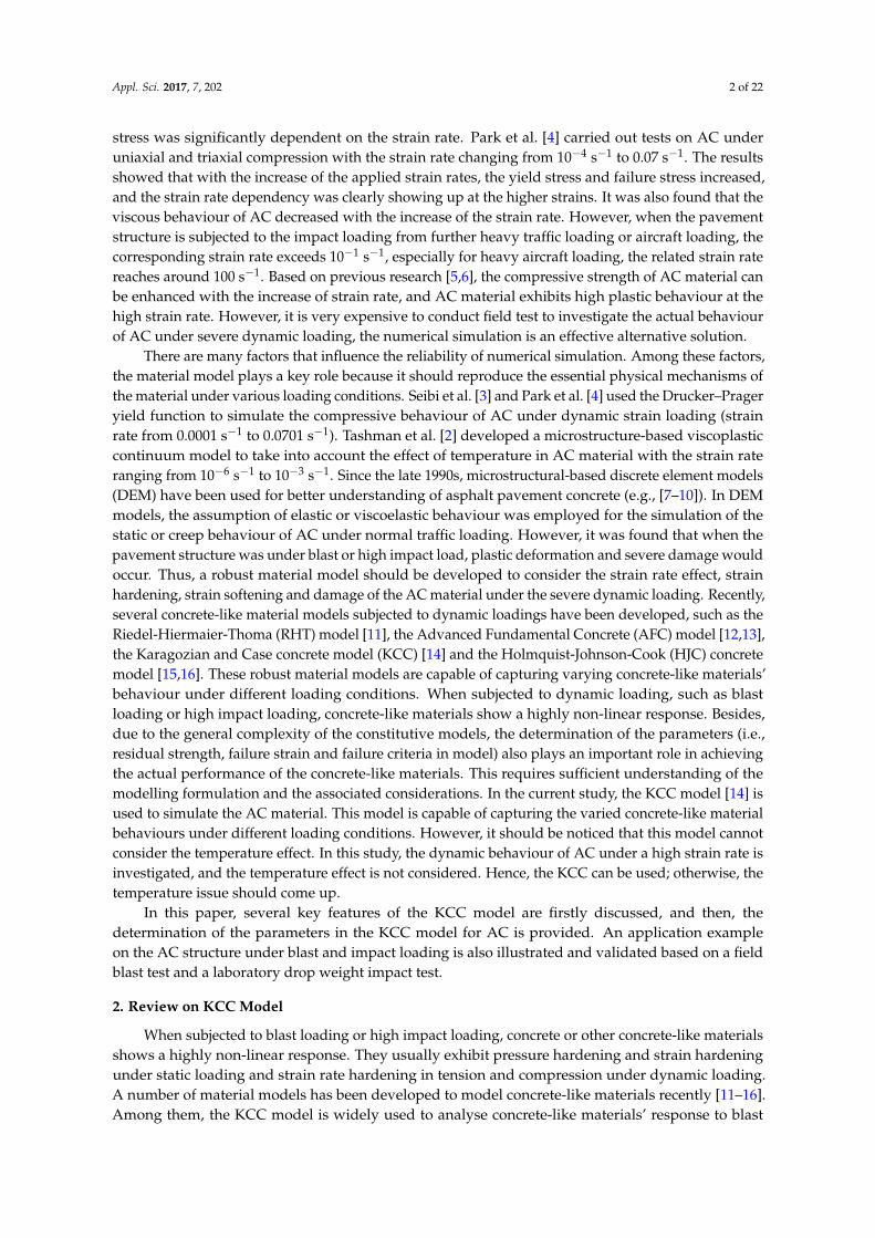
However, for the compressive DIF curve, a numerical modelling of the SHPB test adopting thisDIF curve found that the initial segment of this curve matched the experimental results very well,while the numerical model results for strain rate larger than 100 s−1 seemed to overestimate the stress.This can be due to the “double counting” of the inertia effect in the numerical modelling when thestrain rate exceeded 100 s−1. Hence, in the current model, the second segment in compressive DIF(Equation (19)) is ignored when the strain rate exceeds 100 s−1. Beyond this, the DIF is assumedto remain a constant value. For the tensile DIF curves, in the macro-level numerical model, the

Appl. Sci. 2017, 7, 202 10 of 22

KCC material model cannot capture the aggregate interlocking that propagates the micro-crackingand energy dissipation beyond the localization zone [20–22]. Therefore, the above tensile DIF curve(Equation (20)) with two branches is used in the numerical model. The tensile and compressive DIFcurves of asphalt concrete used in numerical model are summarized in Figure 6.

Appl. Sci. 2017, 7, 202 10 of 23

hydraulic test for AC can be referred to Wu [20]. The DIF value for compressive (DIFc) and tensile (DIFt) strength obtained from the test are given as:

210 103.18 1.098log ( ) 0.1397log ( )dc

csc

fDIFf

ε ε• •

= = + + for 1100sε•

−≤

1021.39log ( ) 36.76dcc

sc

fDIFf

ε•

= = − for 1 1100 200s sε•

− −< ≤ (19)

101.86 0.1432log ( )dtt

st

fDIFf

ε•

= = + for 115sε•

−≤

106.06log ( ) 5.024dtt

st

fDIFf

ε•

= = − for 1 115 100s sε•

− −≤ ≤ (10)

However, for the compressive DIF curve, a numerical modelling of the SHPB test adopting this DIF curve found that the initial segment of this curve matched the experimental results very well, while the numerical model results for strain rate larger than 100 s−1 seemed to overestimate the stress. This can be due to the “double counting” of the inertia effect in the numerical modelling when the strain rate exceeded 100 s−1. Hence, in the current model, the second segment in compressive DIF (Equation (19)) is ignored when the strain rate exceeds 100 s−1. Beyond this, the DIF is assumed to remain a constant value. For the tensile DIF curves, in the macro-level numerical model, the KCC material model cannot capture the aggregate interlocking that propagates the micro-cracking and energy dissipation beyond the localization zone [20–22]. Therefore, the above tensile DIF curve (Equation (20)) with two branches is used in the numerical model. The tensile and compressive DIF curves of asphalt concrete used in numerical model are summarized in Figure 6.

Figure 6. Tensile and compressive dynamic increase factor (DIF) curve used in the numerical model for asphalt concrete.

4. Application Example

4.1. Case for Blast Loading

4.1.1. Field Blast Test

In this section, the AC material is used in the multi-layer pavement. Figure 7 shows the cross-sectional view of the multi-layer pavement slab including 100 mm-thick engineering cementitious composite (ECC) at the bottom, 100 mm-thick high strength concrete (HSC) in the middle and 75 mm-thick AC at the top. The geogrid (GST) was placed at the middle of the AC layer

Strain rate (1/s)

DIF

10-6 10-5 10-4 10-3 10-2 10-1 100 101 102 1030

1

2

3

4

5

6

7

8

Tensile DIFCompressive DIF

Figure 6. Tensile and compressive dynamic increase factor (DIF) curve used in the numerical modelfor asphalt concrete.

4. Application Example

4.1. Case for Blast Loading

4.1.1. Field Blast Test

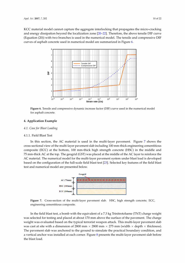
In this section, the AC material is used in the multi-layer pavement. Figure 7 shows thecross-sectional view of the multi-layer pavement slab including 100 mm-thick engineering cementitiouscomposite (ECC) at the bottom, 100 mm-thick high strength concrete (HSC) in the middle and75 mm-thick AC at the top. The geogrid (GST) was placed at the middle of the AC layer to reinforce theAC material. The numerical model for the multi-layer pavement system under blast load is developedbased on the configuration of the full-scale field blast test [23]. Selected key features of the field blasttest and numerical model are presented below.

Appl. Sci. 2017, 7, 202 11 of 23

to reinforce the AC material. The numerical model for the multi-layer pavement system under blast load is developed based on the configuration of the full-scale field blast test [23]. Selected key features of the field blast test and numerical model are presented below.

Figure 7. Cross-section of the multi-layer pavement slab. HSC, high strength concrete; ECC, engineering cementitious composite.

In the field blast test, a bomb with the equivalent of a 7.3 kg Trinitrotoluene (TNT) charge weight was selected for testing and placed at about 170 mm above the surface of the pavement. The charge weight was evaluated based on the typical terrorist weapon attack. This multi-layer pavement slab was cast at site with a dimension of 2800 mm × 2800 mm × 275 mm (width × depth × thickness). The pavement slab was anchored to the ground to simulate the practical boundary condition, and a vertical anchor was installed at each corner. Figure 8 presents the multi-layer pavement slab before the blast load.

Various instruments were installed onto the slab to measure its responses during blast loading. Figure 9 shows the instrumentation installed on the pavement slab. Four accelerometers were installed at the middle of the side of the slab to measure both vertical (V1 and V2 in Figure 9) and horizontal accelerations (H1 and H2 in Figure 9). The accelerometers were mounted onto steel frames that were cast together with the slab. Three total pressure cells (TPC) (TPC1, TPC 2 and TPC3 in Figure 9) were buried in the soil just below the slab to measure the pressure transferred from the pavement slab.

Figure 8. Plan view of the multi-layer pavement slab before the blast event.

A numerical model is established using LSDYNA package [24]. In this model, the slab and foundation soil are discretised in space with one point Gauss integration eight-node hexahedron Lagrange element. Only a quarter of the slab is modelled with symmetric boundary conditions (as shown in Figure 10). The geogrid is spatially discretised with the shell element, and it is assumed that the geogrid is fully bonded within the AC layer. The anchors on the pavement slab are simulated as the fixed points (fixed in vertical direction) in the corresponding position in the numerical model. The non-reflection boundary is applied on the side and bottom of the foundation soil to model semi-infinite space. Based on the mesh study on the numerical model, the 10-mm element size is adopted for the pavement slab, geogrid and soil mass. The blast pressure is extracted from AUTODYN and used for numerical model analysis. The detailed process of applying pressure to the pavement surface can be referred to elsewhere [20,25].

Figure 7. Cross-section of the multi-layer pavement slab. HSC, high strength concrete; ECC,engineering cementitious composite.

In the field blast test, a bomb with the equivalent of a 7.3 kg Trinitrotoluene (TNT) charge weightwas selected for testing and placed at about 170 mm above the surface of the pavement. The chargeweight was evaluated based on the typical terrorist weapon attack. This multi-layer pavement slabwas cast at site with a dimension of 2800 mm × 2800 mm × 275 mm (width × depth × thickness).The pavement slab was anchored to the ground to simulate the practical boundary condition, anda vertical anchor was installed at each corner. Figure 8 presents the multi-layer pavement slab beforethe blast load.

Appl. Sci. 2017, 7, 202 11 of 22

Appl. Sci. 2017, 7, 202 11 of 23

to reinforce the AC material. The numerical model for the multi-layer pavement system under blast load is developed based on the configuration of the full-scale field blast test [23]. Selected key features of the field blast test and numerical model are presented below.

Figure 7. Cross-section of the multi-layer pavement slab. HSC, high strength concrete; ECC, engineering cementitious composite.

In the field blast test, a bomb with the equivalent of a 7.3 kg Trinitrotoluene (TNT) charge weight was selected for testing and placed at about 170 mm above the surface of the pavement. The charge weight was evaluated based on the typical terrorist weapon attack. This multi-layer pavement slab was cast at site with a dimension of 2800 mm × 2800 mm × 275 mm (width × depth × thickness). The pavement slab was anchored to the ground to simulate the practical boundary condition, and a vertical anchor was installed at each corner. Figure 8 presents the multi-layer pavement slab before the blast load.

Various instruments were installed onto the slab to measure its responses during blast loading. Figure 9 shows the instrumentation installed on the pavement slab. Four accelerometers were installed at the middle of the side of the slab to measure both vertical (V1 and V2 in Figure 9) and horizontal accelerations (H1 and H2 in Figure 9). The accelerometers were mounted onto steel frames that were cast together with the slab. Three total pressure cells (TPC) (TPC1, TPC 2 and TPC3 in Figure 9) were buried in the soil just below the slab to measure the pressure transferred from the pavement slab.

Figure 8. Plan view of the multi-layer pavement slab before the blast event.

A numerical model is established using LSDYNA package [24]. In this model, the slab and foundation soil are discretised in space with one point Gauss integration eight-node hexahedron Lagrange element. Only a quarter of the slab is modelled with symmetric boundary conditions (as shown in Figure 10). The geogrid is spatially discretised with the shell element, and it is assumed that the geogrid is fully bonded within the AC layer. The anchors on the pavement slab are simulated as the fixed points (fixed in vertical direction) in the corresponding position in the numerical model. The non-reflection boundary is applied on the side and bottom of the foundation soil to model semi-infinite space. Based on the mesh study on the numerical model, the 10-mm element size is adopted for the pavement slab, geogrid and soil mass. The blast pressure is extracted from AUTODYN and used for numerical model analysis. The detailed process of applying pressure to the pavement surface can be referred to elsewhere [20,25].

Figure 8. Plan view of the multi-layer pavement slab before the blast event.

Various instruments were installed onto the slab to measure its responses during blast loading.Figure 9 shows the instrumentation installed on the pavement slab. Four accelerometers were installedat the middle of the side of the slab to measure both vertical (V1 and V2 in Figure 9) and horizontalaccelerations (H1 and H2 in Figure 9). The accelerometers were mounted onto steel frames that werecast together with the slab. Three total pressure cells (TPC) (TPC1, TPC 2 and TPC3 in Figure 9) wereburied in the soil just below the slab to measure the pressure transferred from the pavement slab.Appl. Sci. 2017, 7, 202 12 of 23

Figure 9. Layout of instrumentation for field blast test. TPC, total pressure cell.

Figure 10. Finite element model of the multi-layer pavement slab.

In the numerical model, AC, ECC and HSC are all grouped as concrete-like materials and modelled by the KCC model [20,23]. The basic parameters for these three materials are listed in Table 3. The parameters for AC material in the KCC model can be found in Section 3. While the process of the determination of HSC and ECC parameters for KCC model is the same as that mentioned in Section 3, the detailed parameters can be referred to Wu [20]. The Drucker–Prager model and plastic-kinematic model [17] are employed to model the foundation soil and geogrid,

Figure 9. Layout of instrumentation for field blast test. TPC, total pressure cell.

A numerical model is established using LSDYNA package [24]. In this model, the slab andfoundation soil are discretised in space with one point Gauss integration eight-node hexahedronLagrange element. Only a quarter of the slab is modelled with symmetric boundary conditions(as shown in Figure 10). The geogrid is spatially discretised with the shell element, and it is assumedthat the geogrid is fully bonded within the AC layer. The anchors on the pavement slab are simulatedas the fixed points (fixed in vertical direction) in the corresponding position in the numerical model.The non-reflection boundary is applied on the side and bottom of the foundation soil to modelsemi-infinite space. Based on the mesh study on the numerical model, the 10-mm element size isadopted for the pavement slab, geogrid and soil mass. The blast pressure is extracted from AUTODYNand used for numerical model analysis. The detailed process of applying pressure to the pavementsurface can be referred to elsewhere [20,25].

Appl. Sci. 2017, 7, 202 12 of 22

Appl. Sci. 2017, 7, 202 12 of 23

Figure 9. Layout of instrumentation for field blast test. TPC, total pressure cell.

Figure 10. Finite element model of the multi-layer pavement slab.

In the numerical model, AC, ECC and HSC are all grouped as concrete-like materials and modelled by the KCC model [20,23]. The basic parameters for these three materials are listed in Table 3. The parameters for AC material in the KCC model can be found in Section 3. While the process of the determination of HSC and ECC parameters for KCC model is the same as that mentioned in Section 3, the detailed parameters can be referred to Wu [20]. The Drucker–Prager model and plastic-kinematic model [17] are employed to model the foundation soil and geogrid,

Figure 10. Finite element model of the multi-layer pavement slab.

In the numerical model, AC, ECC and HSC are all grouped as concrete-like materials andmodelled by the KCC model [20,23]. The basic parameters for these three materials are listed in Table 3.The parameters for AC material in the KCC model can be found in Section 3. While the processof the determination of HSC and ECC parameters for KCC model is the same as that mentionedin Section 3, the detailed parameters can be referred to Wu [20]. The Drucker–Prager model andplastic-kinematic model [17] are employed to model the foundation soil and geogrid, respectively.The AUTOMATIC_SURFACE_TO_SURFACE contact algorithm is employed to model the interactionbetween pavement slab and soil. The TIEBREAK contact algorithm in LSDYNA is used to simulate theinterface behaviour between HSC and AC layers. The parameters for the foundation soil, geogrid andinterface property are in Tables 4–6, respectively.

Table 3. Basic properties of materials in the multi-layer pavement for the blast load.

Parameters AC HSC ECC

Young’s modulus E (MPa) 598 33,000 18,000Compressive strength fc (MPa) 4.6 55 64

Tensile strength ft (MPa) 0.7 4.35 5Poisson ratio ν 0.35 0.2 0.22

Table 4. Parameters for Geogrid MG-100 using the plastic-kinematic model.

Parameters Symbol Units Value

Density ρ kg/m3 1030Young’s modulus E MPa 500

Poisson’s ratio ν - 0.3Yield stress σy MPa 7.5

Tangent modulus Et MPa 333Thickness t mm 2.4

Erosion strain εs - 0.038

Appl. Sci. 2017, 7, 202 13 of 22

Table 5. Material properties of the soil mass.

Parameters Symbol Units Value

Density ρ kg/m3 2100Shear modulus G MPa 13.8Poisson’s ratio ν - 0.3

Cohesion c kPa 62Friction angle φ ◦ 26

Table 6. Parameters for the interface simulation.

Parameters Value

Contact type TIEBREAKFriction for static 0.71

Friction for dynamic 0.56

4.1.2. Numerical Result

The results of the numerical modelling of the multi-layer pavement under blast loading, with theincorporation of the above-mentioned material models, are summarized and compared with the blasttest results. In the numerical results, the fringe level in the damage contour is the value for the scaleddamage indicator δ, which is defined to describe the damage level of the material [14,20,23]. A scaleddamage indicator δ is related to the effective plastic strain λ in the material: (i) at the yield surface,λ = 0, leading to δ = 0; (ii) at the maximum strength surface, λ = λm, leading to δ = 1; and (iii) at theresidual strength surface, λ = λr >> λm, leading to δ = 1.99 ≈ 2. Thus, the δ value moving from 0 to 1 to2 indicates that the failure surface migrates from the yield surface to the maximum strength surfaceand to the residual strength surface, respectively, as the material being stressed. In this study, when theresidual strength of material reduces to 20% of its peak strength, the material seems to suffer severefailure. The plastic strain corresponded to that residual strength used to calculate the delta value. Boththe laboratory and field test for AC material indicated that when δ was greater than 1.8, the materialwould be severely damaged.

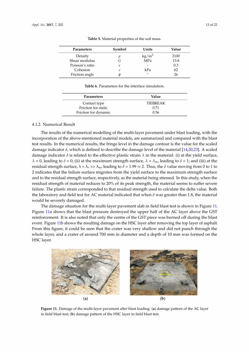
The damage situation for the multi-layer pavement slab in field blast test is shown in Figure 11.Figure 11a shows that the blast pressure destroyed the upper half of the AC layer above the GSTreinforcement. It is also noted that only the centre of the GST piece was burned off during the blastevent. Figure 11b shows the resulting damage on the HSC layer after removing the top layer of asphalt.From this figure, it could be seen that the crater was very shallow and did not punch through thewhole layer, and a crater of around 700 mm in diameter and a depth of 10 mm was formed on theHSC layer.

Appl. Sci. 2017, 7, 202 14 of 23

The damage situation for the multi-layer pavement slab in field blast test is shown in Figure 11. Figure 11a shows that the blast pressure destroyed the upper half of the AC layer above the GST reinforcement. It is also noted that only the centre of the GST piece was burned off during the blast event. Figure 11b shows the resulting damage on the HSC layer after removing the top layer of asphalt. From this figure, it could be seen that the crater was very shallow and did not punch through the whole layer, and a crater of around 700 mm in diameter and a depth of 10 mm was formed on the HSC layer.

(a) (b)

Figure 11. Damage of the multi-layer pavement after blast loading: (a) damage pattern of the AC layer in field blast test; (b) damage pattern of the HSC layer in field blast test.

The damage contour for the AC layer in numerical model is shown in Figure 12a. Comparing Figures 12a and Figure 11a, it is observed that the damage pattern in the numerical model is symmetrical, while that in the field measurement was skewed. This is because the bomb in the field was not placed at the centre of the slab, and one side of the AC layer was more severely damaged than the other. Shear cracking near the anchor point was observed in the numerical model, which was similar to the experimental observations in the field test. It could be concluded that the basic failure pattern given by the numerical model agrees well with the results obtained from the field-testing. Figure 12b shows the damage pattern for the HSC layer. Comparing Figure 12b with Figure 11b, the damage pattern for HSC is very consistent between field measurement and numerical results. The diameter of the crater was about 750 mm in the numerical model, which is very close to that of the blast test result. As shown in Figure 12b, shear cracks are also observed near the anchor points. Based on the damage pattern in the field blast test, the crater on the top face of the HSC is shown to be shallow and with a thickness of less than 10 mm. However, after cracking occurred at the bottom of the HSC layer, the numerical model shows that the bottom of the HSC layer has experienced severe cracking. This might be due to the combination of the bending of the HSC layer under the blast load and the reflection of the stress wave at the bottom interface. In the numerical model, the interface between HSC and ECC is assumed to be fully bonded. However, ECC is more flexible than HSC, and thus, it would cause tensile stress at the bottom of the HSC layer when deformed together. The compression stress wave from the top face would also travel within the HSC layer and reflect as a tension stress at the interface, which could cause spalling. Based on the damage pattern in the numerical model, the HSC layer might be considered having failed, while the field observation suggests that HSC may have partially failed.

In the field blast test, the four accelerometers were installed at the mid-side of pavement slab (as shown in Figure 9). These accelerometers were used to measure the vertical and horizontal acceleration of the pavement slab subjected to blast loading. For the horizontal acceleration, due to the centre of the charge being closer to one side of the pavement slab; there were two different horizontal acceleration readings; while in the numerical model, it was assumed that the explosive occurred in the centre of the pavement slab. Thus, in this section, only the vertical acceleration from the field blast test was compared with that of the numerical model. In the numerical model, the raw nodal acceleration contained considerable numerical noise. The ELEMENT_SEATBELT_ACCELEROMETER could be used to eliminate numerical noise and obtain more accurate node acceleration. The vertical acceleration from the blast testing is compared with that of the numerical model as shown in Table 7.

Figure 11. Damage of the multi-layer pavement after blast loading: (a) damage pattern of the AC layerin field blast test; (b) damage pattern of the HSC layer in field blast test.

Appl. Sci. 2017, 7, 202 14 of 22

The damage contour for the AC layer in numerical model is shown in Figure 12a. ComparingFigures 11a and 12a, it is observed that the damage pattern in the numerical model is symmetrical,while that in the field measurement was skewed. This is because the bomb in the field was not placedat the centre of the slab, and one side of the AC layer was more severely damaged than the other.Shear cracking near the anchor point was observed in the numerical model, which was similar to theexperimental observations in the field test. It could be concluded that the basic failure pattern given bythe numerical model agrees well with the results obtained from the field-testing. Figure 12b showsthe damage pattern for the HSC layer. Comparing Figure 11b with Figure 12b, the damage patternfor HSC is very consistent between field measurement and numerical results. The diameter of thecrater was about 750 mm in the numerical model, which is very close to that of the blast test result.As shown in Figure 12b, shear cracks are also observed near the anchor points. Based on the damagepattern in the field blast test, the crater on the top face of the HSC is shown to be shallow and with athickness of less than 10 mm. However, after cracking occurred at the bottom of the HSC layer, thenumerical model shows that the bottom of the HSC layer has experienced severe cracking. This mightbe due to the combination of the bending of the HSC layer under the blast load and the reflection ofthe stress wave at the bottom interface. In the numerical model, the interface between HSC and ECC isassumed to be fully bonded. However, ECC is more flexible than HSC, and thus, it would cause tensilestress at the bottom of the HSC layer when deformed together. The compression stress wave from thetop face would also travel within the HSC layer and reflect as a tension stress at the interface, whichcould cause spalling. Based on the damage pattern in the numerical model, the HSC layer might beconsidered having failed, while the field observation suggests that HSC may have partially failed.

Appl. Sci. 2017, 7, 202 15 of 23

The results from both the blast testing and the numerical simulation are comparable. The maximum difference of vertical acceleration between the blast testing and the numerical model is about 10%, and the numerical model predicted slightly higher in the vertical acceleration than that of the blast test.

(a) (b)

Figure 12. Damage contour for the AC and HSC layer in the multi-layers pavement: (a) damage contour of the AC layer in the numerical simulation; (b) damage contour of the HSC layer in the numerical simulation.

Table 7. Vertical acceleration of the multi-layer pavement slab.

Item Field Trial Test Numerical Result Deviation from Field Trial Test Max. vertical

acceleration (m/s2) 35,400 38,870 10%

The pressure values in the corresponding points in the numerical model are compared with pressures obtained from the blast test, as summarized in Table 8. The layout of the total pressure cell in the blast could be referred to Figure 9. The pressure values from the numerical simulation are shown to be close to that from the blast test for TPC2; while for TPC3, it has a 20% discrepancy with the numerical simulation considering the inherent variation in the blast test. TPC1 was damaged during the blast test, and hence, no pressure reading was recorded from it. The numerical model predicts that the pressure might be as high as 13 MPa at that point, which is far beyond the maximum measurement capacity of the pressure cell installed. That can explain why TPC1 was destroyed due to the overwhelming blast loading.

Table 8. Peak reading for the total pressure cell.

Item Field Blast Test (kPa) Numerical Result (kPa) Deviation from Field Trial Test

TPC1 Destroyed 13,393 Sensor destroyed as pressure >> range

TPC2 273 267 2% TPC3 200 241 20%

Figure 12. Damage contour for the AC and HSC layer in the multi-layers pavement: (a) damagecontour of the AC layer in the numerical simulation; (b) damage contour of the HSC layer in thenumerical simulation.

In the field blast test, the four accelerometers were installed at the mid-side of pavement slab(as shown in Figure 9). These accelerometers were used to measure the vertical and horizontalacceleration of the pavement slab subjected to blast loading. For the horizontal acceleration, due to thecentre of the charge being closer to one side of the pavement slab; there were two different horizontalacceleration readings; while in the numerical model, it was assumed that the explosive occurred inthe centre of the pavement slab. Thus, in this section, only the vertical acceleration from the field

Appl. Sci. 2017, 7, 202 15 of 22

blast test was compared with that of the numerical model. In the numerical model, the raw nodalacceleration contained considerable numerical noise. The ELEMENT_SEATBELT_ACCELEROMETERcould be used to eliminate numerical noise and obtain more accurate node acceleration. The verticalacceleration from the blast testing is compared with that of the numerical model as shown in Table 7.The results from both the blast testing and the numerical simulation are comparable. The maximumdifference of vertical acceleration between the blast testing and the numerical model is about 10%, andthe numerical model predicted slightly higher in the vertical acceleration than that of the blast test.

Table 7. Vertical acceleration of the multi-layer pavement slab.

Item Field Trial Test Numerical Result Deviation from Field Trial Test

Max. verticalacceleration (m/s2) 35,400 38,870 10%

The pressure values in the corresponding points in the numerical model are compared withpressures obtained from the blast test, as summarized in Table 8. The layout of the total pressurecell in the blast could be referred to Figure 9. The pressure values from the numerical simulation areshown to be close to that from the blast test for TPC2; while for TPC3, it has a 20% discrepancy withthe numerical simulation considering the inherent variation in the blast test. TPC1 was damagedduring the blast test, and hence, no pressure reading was recorded from it. The numerical modelpredicts that the pressure might be as high as 13 MPa at that point, which is far beyond the maximummeasurement capacity of the pressure cell installed. That can explain why TPC1 was destroyed due tothe overwhelming blast loading.

Table 8. Peak reading for the total pressure cell.

Item Field Blast Test (kPa) Numerical Result (kPa) Deviation from Field Trial Test

TPC1 Destroyed 13,393 Sensor destroyed as pressure >> rangeTPC2 273 267 2%TPC3 200 241 20%

4.2. Case for Impact Loading

4.2.1. Laboratory Drop Weight Impact

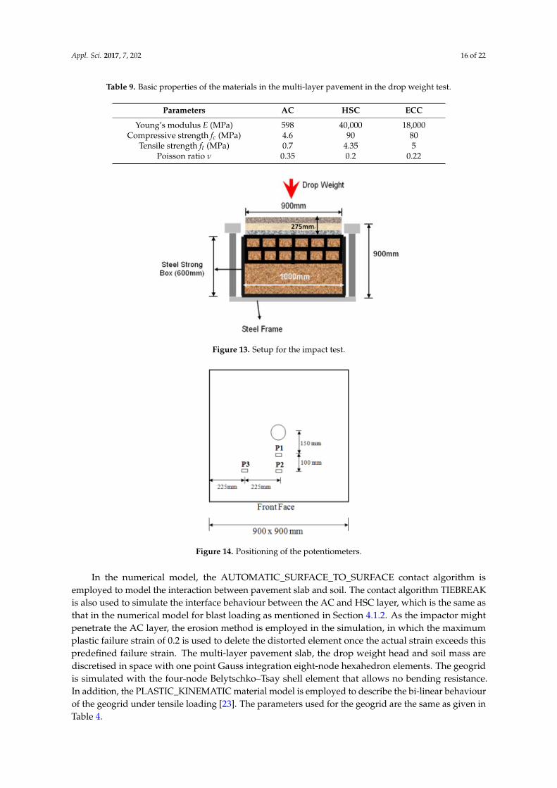
The multi-layer pavement slab was subjected to an 1181-kg drop weight impact. The cross-sectionof the multi-layer pavement is the same as that given in Figure 7. The basic mechanical properties ofthe, HSC, ECC and AC are determined according to ASTM standards, and the results are summarizedin Table 9. The drop weight was a cylindrical projectile with a hemispheric head (100 mm in diameterand made with high strength steel), and the pavement slab was subjected to two times of impact fromthe same drop height of 1.5 m. During the test, the multi-layer pavement slab was placed on the top ofcompacted soil/sand in a steel strong box. Directly below the slab was the geocell (MiraCell MC-100)which was filled with compacted soil/sand. This was to enhance the strength of the soil/sand layerand to provide a solid sub-base as to simulate the practical condition. The setup for the multi-layerpavement slab is given in Figure 13. Various instruments were also installed to monitor the responseof the pavement during the drop weight test. Figure 14 shows the positioning of the potentiometers.A photodiode system was used to trigger the data acquisition system during the test. It consists oftwo photodiodes and two laser sources placed 100 mm vertically apart. The data acquisition systemwould be triggered when the falling projectile crosses the top laser emitter. Impact velocity could bedetermined using the time interval that the projectile took to cross the second laser emitter.

Appl. Sci. 2017, 7, 202 16 of 22

Table 9. Basic properties of the materials in the multi-layer pavement in the drop weight test.

Parameters AC HSC ECC

Young’s modulus E (MPa) 598 40,000 18,000Compressive strength fc (MPa) 4.6 90 80

Tensile strength ft (MPa) 0.7 4.35 5Poisson ratio ν 0.35 0.2 0.22

Appl. Sci. 2017, 7, 202 16 of 23

4.2. Case for Impact Loading

4.2.1. Laboratory Drop Weight Impact

The multi-layer pavement slab was subjected to an 1181-kg drop weight impact. The cross-section of the multi-layer pavement is the same as that given in Figure 7. The basic mechanical properties of the, HSC, ECC and AC are determined according to ASTM standards, and the results are summarized in Table 9. The drop weight was a cylindrical projectile with a hemispheric head (100 mm in diameter and made with high strength steel), and the pavement slab was subjected to two times of impact from the same drop height of 1.5 m. During the test, the multi-layer pavement slab was placed on the top of compacted soil/sand in a steel strong box. Directly below the slab was the geocell (MiraCell MC-100) which was filled with compacted soil/sand. This was to enhance the strength of the soil/sand layer and to provide a solid sub-base as to simulate the practical condition. The setup for the multi-layer pavement slab is given in Figure 13. Various instruments were also installed to monitor the response of the pavement during the drop weight test. Figure 14 shows the positioning of the potentiometers. A photodiode system was used to trigger the data acquisition system during the test. It consists of two photodiodes and two laser sources placed 100 mm vertically apart. The data acquisition system would be triggered when the falling projectile crosses the top laser emitter. Impact velocity could be determined using the time interval that the projectile took to cross the second laser emitter.

Table 9. Basic properties of the materials in the multi-layer pavement in the drop weight test.

Parameters AC HSC ECC Young’s modulus E (MPa) 598 40,000 18,000

Compressive strength fc (MPa) 4.6 90 80 Tensile strength ft (MPa) 0.7 4.35 5

Poisson ratio ν 0.35 0.2 0.22

Figure 13. Setup for the impact test.

In the numerical model, the AUTOMATIC_SURFACE_TO_SURFACE contact algorithm is employed to model the interaction between pavement slab and soil. The contact algorithm TIEBREAK is also used to simulate the interface behaviour between the AC and HSC layer, which is the same as that in the numerical model for blast loading as mentioned in Section 4.1.2. As the impactor might penetrate the AC layer, the erosion method is employed in the simulation, in which the maximum plastic failure strain of 0.2 is used to delete the distorted element once the actual strain exceeds this predefined failure strain. The multi-layer pavement slab, the drop weight head and soil mass are discretised in space with one point Gauss integration eight-node hexahedron elements. The geogrid is simulated with the four-node Belytschko–Tsay shell element that allows

Figure 13. Setup for the impact test.

Appl. Sci. 2017, 7, 202 17 of 23

no bending resistance. In addition, the PLASTIC_KINEMATIC material model is employed to describe the bi-linear behaviour of the geogrid under tensile loading [23]. The parameters used for the geogrid are the same as given in Table 4.

Figure 14. Positioning of the potentiometers.

The Drucker–Prager model is used to simulate soil mass. In the laboratory drop weight test, the upper soil layers were compacted and reinforced with geocell material, which would enhance the strength of the soil, and the lower layer has no reinforcement. Hence, in the numerical model, it is necessary to consider the function of the geocell material. From the laboratory test on the geocell-encased sand [26], it is observed that the geocell confinement did not change the friction angle of soil while significant cohesion occurred in the granular soil, which indicated that for the geocell-reinforced sand layer, the strength and stiffness behaviour of the soil would be enhanced. However, in the numerical model, it is difficult to model and mesh the geocell material due to its complex geometry. Hence, it would be preferable to use the composite model to consider the enhancement of the shear strength and stiffness of the geocell-reinforced sand layer. Madhavi et al. [27] purposed an empirical equation to calculate Young’s modulus of the geocell-reinforced sand using the secant tensile modulus of the geocell material and Young’s modulus parameter of the unreinforced sand, which could be expressed as:

( ) ( )0.7 0.1634 200r uE K Mσ= + (21)

in which 𝐸𝐸𝑟𝑟 is the Young’s modulus of the geocell-reinforced sand, M is the secant modulus of the geocell material at axial strain 2.5% in kN/m and 𝜎𝜎3 is the confining pressure from the geocell in kPa. 𝑘𝑘𝑢𝑢 is the dimensionless modulus parameter of the unreinforced sand, which is a modulus number in the hyperbolic model developed by Duncan and Chang [28]. The confining pressure 𝜎𝜎3 could be calculated as:

30

1 121

a

a

MD

εσ

ε

− −= −

(22)

where 𝐷𝐷0 is the initial diameter of the geocell and 𝜀𝜀𝑎𝑎 is the axial strain of the geocell at failure; the induced cohesion in the geocell-reinforced sand is then related to the increase in the confining pressure 𝜎𝜎3:

3

2r Pc Kσ

= (23)

in which 𝑐𝑐𝑟𝑟 is the enhanced cohesion and 𝑘𝑘𝑝𝑝 is the coefficient of passive earth pressure.

Figure 14. Positioning of the potentiometers.

In the numerical model, the AUTOMATIC_SURFACE_TO_SURFACE contact algorithm isemployed to model the interaction between pavement slab and soil. The contact algorithm TIEBREAKis also used to simulate the interface behaviour between the AC and HSC layer, which is the same asthat in the numerical model for blast loading as mentioned in Section 4.1.2. As the impactor mightpenetrate the AC layer, the erosion method is employed in the simulation, in which the maximumplastic failure strain of 0.2 is used to delete the distorted element once the actual strain exceeds thispredefined failure strain. The multi-layer pavement slab, the drop weight head and soil mass arediscretised in space with one point Gauss integration eight-node hexahedron elements. The geogridis simulated with the four-node Belytschko–Tsay shell element that allows no bending resistance.In addition, the PLASTIC_KINEMATIC material model is employed to describe the bi-linear behaviourof the geogrid under tensile loading [23]. The parameters used for the geogrid are the same as given inTable 4.

Appl. Sci. 2017, 7, 202 17 of 22

The Drucker–Prager model is used to simulate soil mass. In the laboratory drop weight test,the upper soil layers were compacted and reinforced with geocell material, which would enhancethe strength of the soil, and the lower layer has no reinforcement. Hence, in the numerical model,it is necessary to consider the function of the geocell material. From the laboratory test on thegeocell-encased sand [26], it is observed that the geocell confinement did not change the frictionangle of soil while significant cohesion occurred in the granular soil, which indicated that for thegeocell-reinforced sand layer, the strength and stiffness behaviour of the soil would be enhanced.However, in the numerical model, it is difficult to model and mesh the geocell material due toits complex geometry. Hence, it would be preferable to use the composite model to consider theenhancement of the shear strength and stiffness of the geocell-reinforced sand layer. Madhavi et al. [27]purposed an empirical equation to calculate Young’s modulus of the geocell-reinforced sand using thesecant tensile modulus of the geocell material and Young’s modulus parameter of the unreinforcedsand, which could be expressed as:

Er = 4(σ3)0.7(

Ku + 200M0.16)

(21)

in which Er is the Young’s modulus of the geocell-reinforced sand, M is the secant modulus of thegeocell material at axial strain 2.5% in kN/m and σ3 is the confining pressure from the geocell in kPa.ku is the dimensionless modulus parameter of the unreinforced sand, which is a modulus numberin the hyperbolic model developed by Duncan and Chang [28]. The confining pressure σ3 could becalculated as:

σ3 =2MD0

(1−√

1− εa

1− εa

)(22)

where D0 is the initial diameter of the geocell and εa is the axial strain of the geocell at failure;the induced cohesion in the geocell-reinforced sand is then related to the increase in the confiningpressure σ3:

cr =σ3

2

√KP (23)

in which cr is the enhanced cohesion and kp is the coefficient of passive earth pressure.In the current study, the geocell MC-100 from Polyfelt is used. The geocell dimension is a rhombus

with two diagonal lengths of 203 mm and 244 mm. Thus, the equivalent diameter is calculated as about177.5 mm. The secant modulus M for the geocell is obtained as 278 kN/m from the tensile test [20].Additionally, the value of εa is taken as 4.8%. The modulus parameter ku for unreinforced sand inthe current study is taken as 727 MPa according to the curve fitting from the triaxial test, and hence,the confining pressure, enhanced cohesion and Young’s modulus for geocell-reinforced sand couldbe calculated based on Equations (21)–(23). The parameters for the unreinforced sand and geocellreinforced sand are summarized in Table 10.

Table 10. Material properties of the foundation soil.

Parameters Reinforced Sand Layer Unreinforced Sand Layer

Density, ρ (kg/m3) 1600 1600Young’s modulus E (MPa) 103.5 40Shear modulus, G (MPa) 39.8 15.4

Poisson’s ratio, ν 0.3 0.3Cohesion, c (MPa) 0.089 0.001

Friction angle, φ (◦) 40 40

During the impact test, the deformation of the drop weight head was negligible compared to thedeformation of the pavement slab. Hence, the drop weight head is modelled with a rigid body in thecurrent study. For the configuration of the drop weight head, the simple cylindrical shape is modelledinstead of modelling the head with weight mass (as shown in Figure 15). The simple cylindrical head

Appl. Sci. 2017, 7, 202 18 of 22

has a diameter of 100 mm with a length of 1292 mm. The total mass for the simple cylindrical head isabout 1181 kg, from which the density of the drop head would be obtained. The properties for the drophead are listed in Table 11. The convergence study is conducted, and it was found that a 5-mm elementsize gave a stable response, which is therefore applied for the simulation. The numerical model of themulti-layer pavement slab under drop weight impact load is given in Figure 16.

Appl. Sci. 2017, 7, 202 18 of 23

In the current study, the geocell MC-100 from Polyfelt is used. The geocell dimension is a rhombus with two diagonal lengths of 203 mm and 244 mm. Thus, the equivalent diameter is calculated as about 177.5 mm. The secant modulus M for the geocell is obtained as 278 kN/m from the tensile test [20]. Additionally, the value of 𝜀𝜀𝑎𝑎 is taken as 4.8%. The modulus parameter 𝑘𝑘𝑢𝑢 for unreinforced sand in the current study is taken as 727 MPa according to the curve fitting from the triaxial test, and hence, the confining pressure, enhanced cohesion and Young’s modulus for geocell-reinforced sand could be calculated based on Equations (21)–(23). The parameters for the unreinforced sand and geocell reinforced sand are summarized in Table 10.

Table 10. Material properties of the foundation soil.

Parameters Reinforced Sand Layer Unreinforced Sand Layer Density, ρ (kg/m3) 1600 1600

Young’s modulus E (MPa) 103.5 40 Shear modulus, G (MPa) 39.8 15.4

Poisson’s ratio, ν 0.3 0.3 Cohesion, c (MPa) 0.089 0.001

Friction angle, φ (°) 40 40

During the impact test, the deformation of the drop weight head was negligible compared to the deformation of the pavement slab. Hence, the drop weight head is modelled with a rigid body in the current study. For the configuration of the drop weight head, the simple cylindrical shape is modelled instead of modelling the head with weight mass (as shown in Figure 15). The simple cylindrical head has a diameter of 100 mm with a length of 1292 mm. The total mass for the simple cylindrical head is about 1181 kg, from which the density of the drop head would be obtained. The properties for the drop head are listed in Table 11. The convergence study is conducted, and it was found that a 5-mm element size gave a stable response, which is therefore applied for the simulation. The numerical model of the multi-layer pavement slab under drop weight impact load is given in Figure 16.

(a) (b)

Figure 15. Configuration of the drop weight head (quarter model): (a) standard configuration; (b) simple configuration.

Table 11. Properties of the drop weight head.

Parameters Drop-Weight Head Young’s modulus, E (GPa) 207

Yield stress, fy (MPa) 500 Poisson ratio, ν 0.3

Density, ρ (kg/m3) 118,000

Figure 15. Configuration of the drop weight head (quarter model): (a) standard configuration;(b) simple configuration.

Appl. Sci. 2017, 7, 202 19 of 23

Figure 16. Numerical model for a multi-layer pavement slab under drop weight impact (quarter model).

For the 1.5-m drop weight impact, the drop weight head is assigned with 5.02 m/s for the first impact. For the second impact, due to the penetration of the AC layer in the first impact, the distance between the laser diode system and the face of the pavement slab is increased, while in the numerical model, the impact head is just placed at the position right before reaching the surface. Hence, the initial velocity in numerical model for the second impact is determined as the sum of the experimental recorded velocity and velocity caused by gravity acceleration. Thus, the velocity is calculated as 5.06 m/s for the second impact with the gravity acceleration of 9.8 m/s2.

After the first impact, the fully restarted method in LSDYNA is used to conduct the second impact simulation. At the beginning of the second impact, the stress and residual velocity within the pavement slab and the velocity from the first impact are set to be zero. The damage factor and plastic strain is retained in order to check the accumulated damaged behaviour after the second impact. The simulation of the second impact is carried out when the downward velocity of impactor reached zero, as it is very time consuming to continue to simulate the vibration of pavement slab after impact. It should be noticed that the pavement slab stopped rebounding, which might bring numerical errors (i.e., energy unbalance).

4.2.2. Numerical Result

The damaged situations for the multi-layer slab under the first drop weight impact for the experiment and numerical model are presented in Figure 17. It is found from the numerical simulation that the AC layer is penetrated through, and the drop weight head is impeded by the HSC layer due to the high compressive strength. Such findings from the numerical model are consistent with the observation in the physical test. It is observed that no severe and moderate damage happened in the ECC layer. Additionally, the integrity of both HSC and ECC layers is kept after the first impact.

Figure 16. Numerical model for a multi-layer pavement slab under drop weight impact (quarter model).

Table 11. Properties of the drop weight head.

Parameters Drop-Weight Head

Young’s modulus, E (GPa) 207Yield stress, fy (MPa) 500

Poisson ratio, ν 0.3Density, ρ (kg/m3) 118,000

Appl. Sci. 2017, 7, 202 19 of 22

For the 1.5-m drop weight impact, the drop weight head is assigned with 5.02 m/s for the firstimpact. For the second impact, due to the penetration of the AC layer in the first impact, the distancebetween the laser diode system and the face of the pavement slab is increased, while in the numericalmodel, the impact head is just placed at the position right before reaching the surface. Hence, the initialvelocity in numerical model for the second impact is determined as the sum of the experimentalrecorded velocity and velocity caused by gravity acceleration. Thus, the velocity is calculated as5.06 m/s for the second impact with the gravity acceleration of 9.8 m/s2.

After the first impact, the fully restarted method in LSDYNA is used to conduct the secondimpact simulation. At the beginning of the second impact, the stress and residual velocity withinthe pavement slab and the velocity from the first impact are set to be zero. The damage factor andplastic strain is retained in order to check the accumulated damaged behaviour after the second impact.The simulation of the second impact is carried out when the downward velocity of impactor reachedzero, as it is very time consuming to continue to simulate the vibration of pavement slab after impact.It should be noticed that the pavement slab stopped rebounding, which might bring numerical errors(i.e., energy unbalance).

4.2.2. Numerical Result

The damaged situations for the multi-layer slab under the first drop weight impact for theexperiment and numerical model are presented in Figure 17. It is found from the numerical simulationthat the AC layer is penetrated through, and the drop weight head is impeded by the HSC layer dueto the high compressive strength. Such findings from the numerical model are consistent with theobservation in the physical test. It is observed that no severe and moderate damage happened in theECC layer. Additionally, the integrity of both HSC and ECC layers is kept after the first impact.Appl. Sci. 2017, 7, 202  20 of 23 

(a)  (b)

Figure 17. Damage of  the multi‐layer slab after  the  first  impact:  (a) damage pattern of slab  in  the 

laboratory test; (b) damage pattern of slab in the numerical simulation. 

The damage situations for the multi‐layer pavement slab under the second drop weight impact 

and the numerical model are given in Figure 18. The simulation results indicate that the HSC layer 

stopped the impactor; however, severe damage happens at the top surface and in the middle at the 

side of the HSC layer. Severe damage occurs at the rear surface of the HSC layer, as well. For the 

ECC layer, it is shown that the cracking occurs and propagates from the centre at the top surface. 

However, the damage area is smaller than that of the HSC layer. The cracks are also found in the 

middle at  the side of  the ECC  layer, and similar  to  the experiment,  the crack does not propagate 

through the thickness of the layer. Figure 19 compares the numerical results with the experimental 

results about  the  rear  surface of ECC  layer after  the  second  impact  for  the multi‐layer  slab.  It  is 

found that the damaged contour and cracking pattern were similar. Such results further indicate the 

reasonable close agreement between the numerical analysis and the experimental results using the 

KCC model for AC material. 

(a)  (b)

Figure 18. Damage of multi‐layer  slab after  the  second  impact:  (a) damage pattern of  slab  in  the 

laboratory test; (b) damage pattern of slab in the numerical simulation. 

Table 12  compares  the numerical  results with  the experimental data  for  the multi‐layer  slab 

under  two  times  of  the  drop  weight  impact.  After  the  first  impact,  the  settlement  from  the 

numerical results  is close  to  that obtained  from  the experiment at P2. A big deviation  is  found  in 

between  the  numerical  results  and  experiment  results  on  the  settlement  at  P3.  This might  be 

attributed  to  the  dislocation  of  the  potentiometer  at  P3  upon  impact,  which  could  lead  to  a 

misreporting of  the  settlement  at P3.  In  addition,  the  settlement  at P1  is  lower  in  the numerical 

results compared with the experimental results. This could be attributed to the erosion process  in 

the numerical model or, more specifically, the energy released phenomena. At the second impact, 

since  no  erosion  technology  is  employed  for  the  HSC  layer,  the  numerical  results  are  more 

reasonable.  In  the  impact  simulation,  the  HSC  layer  suffered  deformation  instead  of  being 

penetrated, and hence, no erosion technique was adopted to trigger the energy released phenomena. 

Asphalt Layer Intact

Small Crater

Cracks radiating out from Crater

Figure 17. Damage of the multi-layer slab after the first impact: (a) damage pattern of slab in thelaboratory test; (b) damage pattern of slab in the numerical simulation.

The damage situations for the multi-layer pavement slab under the second drop weight impactand the numerical model are given in Figure 18. The simulation results indicate that the HSC layerstopped the impactor; however, severe damage happens at the top surface and in the middle at the sideof the HSC layer. Severe damage occurs at the rear surface of the HSC layer, as well. For the ECC layer,it is shown that the cracking occurs and propagates from the centre at the top surface. However, thedamage area is smaller than that of the HSC layer. The cracks are also found in the middle at the sideof the ECC layer, and similar to the experiment, the crack does not propagate through the thickness ofthe layer. Figure 19 compares the numerical results with the experimental results about the rear surfaceof ECC layer after the second impact for the multi-layer slab. It is found that the damaged contour andcracking pattern were similar. Such results further indicate the reasonable close agreement betweenthe numerical analysis and the experimental results using the KCC model for AC material.

Appl. Sci. 2017, 7, 202 20 of 22

Appl. Sci. 2017, 7, 202  20 of 23 

(a)  (b)

Figure 17. Damage of  the multi‐layer slab after  the  first  impact:  (a) damage pattern of slab  in  the 

laboratory test; (b) damage pattern of slab in the numerical simulation. 

The damage situations for the multi‐layer pavement slab under the second drop weight impact 

and the numerical model are given in Figure 18. The simulation results indicate that the HSC layer 

stopped the impactor; however, severe damage happens at the top surface and in the middle at the 

side of the HSC layer. Severe damage occurs at the rear surface of the HSC layer, as well. For the 

ECC layer, it is shown that the cracking occurs and propagates from the centre at the top surface. 

However, the damage area is smaller than that of the HSC layer. The cracks are also found in the 

middle at  the side of  the ECC  layer, and similar  to  the experiment,  the crack does not propagate 

through the thickness of the layer. Figure 19 compares the numerical results with the experimental 

results about  the  rear  surface of ECC  layer after  the  second  impact  for  the multi‐layer  slab.  It  is 

found that the damaged contour and cracking pattern were similar. Such results further indicate the 

reasonable close agreement between the numerical analysis and the experimental results using the 

KCC model for AC material. 

(a)  (b)

Figure 18. Damage of multi‐layer  slab after  the  second  impact:  (a) damage pattern of  slab  in  the 

laboratory test; (b) damage pattern of slab in the numerical simulation. 

Table 12  compares  the numerical  results with  the experimental data  for  the multi‐layer  slab 

under  two  times  of  the  drop  weight  impact.  After  the  first  impact,  the  settlement  from  the 

numerical results  is close  to  that obtained  from  the experiment at P2. A big deviation  is  found  in 

between  the  numerical  results  and  experiment  results  on  the  settlement  at  P3.  This might  be 

attributed  to  the  dislocation  of  the  potentiometer  at  P3  upon  impact,  which  could  lead  to  a 

misreporting of  the  settlement  at P3.  In  addition,  the  settlement  at P1  is  lower  in  the numerical 

results compared with the experimental results. This could be attributed to the erosion process  in 

the numerical model or, more specifically, the energy released phenomena. At the second impact, 

since  no  erosion  technology  is  employed  for  the  HSC  layer,  the  numerical  results  are  more 

reasonable.  In  the  impact  simulation,  the  HSC  layer  suffered  deformation  instead  of  being 

penetrated, and hence, no erosion technique was adopted to trigger the energy released phenomena. 

Asphalt Layer Intact

Small Crater

Cracks radiating out from Crater

Figure 18. Damage of multi-layer slab after the second impact: (a) damage pattern of slab in thelaboratory test; (b) damage pattern of slab in the numerical simulation.

Appl. Sci. 2017, 7, 202  21 of 23 

Thus, the settlement profile of the pavement slab decreased with the increase of the radial distance 

from the centre, which indicated that the whole pavement slab bent during the impact. In general, 

the  numerical models  provide  reasonable  estimations  on  the  settlements  of  the multi‐layer  slab 

under  impacts,  in  particular  under  the  second  impact  load,  though  discrepancies  exist  at   

certain regions. 

 (a)  (b)

Figure 19. ECC bottom after the second  impact: (a) damage pattern of the bottom of ECC  layer  in 

the laboratory test; (b) damage pattern of the bottom of ECC layer in the numerical simulation. 

Table  12.  Summary  of  the  settlements  of  the  multi‐layer  slab  from  both  numerical  and   

experiment results. 

Potentiometer 

1st Impact 2nd Impact 

Test 

Result 

FE 

Results FE/Test 

Test 

Result 

FE 

Results FE/Test 

P1 (mm)  ‐‐‐  −1.54  ‐‐‐  −3.62  −7.62  2.10 

P2 (mm)  −1.81  −1.70  0.94  −7.60  −6.63  0.87 

P3 (mm)  −5.27  −1.86  0.35  −5.58  −4.83  0.87 

−ve → downwards 

5. Conclusions 

In this paper, the formulations of strength surfaces and damage  factor  in  the KCC model are 

discussed and evaluated.  It  is  found  that  the KCC model would  reproduce  the  real behaviour of 

concrete‐like  material  under  severe  loadings,  such  as  blast  and  impact  loadings.  Then,  the  key 

parameters controlling the behaviour of AC material under dynamic loadings are discussed, and the 

parameters of AC materials using the KCC model are determined by laboratory static and dynamic 

tests. The proposed damage  factor  in  this paper results  in smoother descending  than  the original 

damage factor and also a higher failure strain that could improve the simulation of the behaviour of 

AC material.  Furthermore,  the  numerical modelling  of multi‐layer  pavement,  in  which  the AC 

material  served as  the  surface  layer, under blast and  impact  loading  is conducted using the KCC 

model. These results are compared with that of the field blast test and the laboratory drop weight 

impact tests, and it is found that the KCC model for the AC material can reproduce the real material 

behaviour under blast and impact loading. 

Acknowledgments:  Part  of  this  research was  sponsored by  the National Basic Research Program  of China   

(No. 2015CB058003),  the Beijing Municipal Natural Science Foundation (No. 8172010) and the Youth Teacher 

Training Scheme from the Shanghai Education Committee (No. ZZGCD15053). Thanks are given here. 

 

Figure 19. ECC bottom after the second impact: (a) damage pattern of the bottom of ECC layer in thelaboratory test; (b) damage pattern of the bottom of ECC layer in the numerical simulation.

Table 12 compares the numerical results with the experimental data for the multi-layer slab undertwo times of the drop weight impact. After the first impact, the settlement from the numerical resultsis close to that obtained from the experiment at P2. A big deviation is found in between the numericalresults and experiment results on the settlement at P3. This might be attributed to the dislocationof the potentiometer at P3 upon impact, which could lead to a misreporting of the settlement at P3.In addition, the settlement at P1 is lower in the numerical results compared with the experimentalresults. This could be attributed to the erosion process in the numerical model or, more specifically,the energy released phenomena. At the second impact, since no erosion technology is employed forthe HSC layer, the numerical results are more reasonable. In the impact simulation, the HSC layersuffered deformation instead of being penetrated, and hence, no erosion technique was adopted totrigger the energy released phenomena. Thus, the settlement profile of the pavement slab decreasedwith the increase of the radial distance from the centre, which indicated that the whole pavementslab bent during the impact. In general, the numerical models provide reasonable estimations on thesettlements of the multi-layer slab under impacts, in particular under the second impact load, thoughdiscrepancies exist at certain regions.

Appl. Sci. 2017, 7, 202 21 of 22

Table 12. Summary of the settlements of the multi-layer slab from both numerical and experiment results.

Potentiometer1st Impact 2nd Impact

Test Result FE Results FE/Test Test Result FE Results FE/Test

P1 (mm) — −1.54 — −3.62 −7.62 2.10P2 (mm) −1.81 −1.70 0.94 −7.60 −6.63 0.87P3 (mm) −5.27 −1.86 0.35 −5.58 −4.83 0.87

−ve→ downwards

5. Conclusions

In this paper, the formulations of strength surfaces and damage factor in the KCC model arediscussed and evaluated. It is found that the KCC model would reproduce the real behaviour ofconcrete-like material under severe loadings, such as blast and impact loadings. Then, the keyparameters controlling the behaviour of AC material under dynamic loadings are discussed, and theparameters of AC materials using the KCC model are determined by laboratory static and dynamictests. The proposed damage factor in this paper results in smoother descending than the originaldamage factor and also a higher failure strain that could improve the simulation of the behaviourof AC material. Furthermore, the numerical modelling of multi-layer pavement, in which the ACmaterial served as the surface layer, under blast and impact loading is conducted using the KCC model.These results are compared with that of the field blast test and the laboratory drop weight impact tests,and it is found that the KCC model for the AC material can reproduce the real material behaviourunder blast and impact loading.

Acknowledgments: Part of this research was sponsored by the National Basic Research Program of China(No. 2015CB058003), the Beijing Municipal Natural Science Foundation (No. 8172010) and the Youth TeacherTraining Scheme from the Shanghai Education Committee (No. ZZGCD15053). Thanks are given here.

Author Contributions: Jun Wu conceived of and designed the experiments. Jun Wu performed the experimentsand analysed the data. Liang Li developed the numerical model and prepared the paper. Xiuli Du discussed thenumerical results and provided a suggestion on the overall organization of the paper. Xuemei Liu conducted thenumerical model of the SHPB test for concrete-like materials and revised the manuscript.

Conflicts of Interest: The authors declare no conflict of interest.

References

1. Huang, Y.H. Pavement Analysis and Design; Pearson Education, Inc.: Upper Saddle River, NJ, USA, 2004.2. Tashman, L.; Masad, E.; Little, D.; Zbib, H. A Microstructure-Based Viscoplastic Model for Asphalt Concrete.

Int. J. Plast. 2005, 21, 1659–1685. [CrossRef]3. Seibi, A.C.; Sharma, M.; Ali, G.; Kenis, W.J. Constitutive Relations for Asphalt Concrete under High Rates

of Loading. Transp. Res. Rec. 2001, 1767, 111–119. [CrossRef]4. Park, D.W.; Martin, A.E.; Lee, H.S.; Masad, E. Characterization of Permanent Deformation of an Asphalt

Mixture Using a Mechanistic Approach. KSCE J. Civ. Eng. 2005, 9, 213–218. [CrossRef]5. Tang, W.; Ding, Y.; Yuan, X. The HJC Model Parameters of an Asphalt Mixture. In Proceedings of the 9th

International Conference on the Mechanical and Physical Behaviour of Materials under Dynamic Loading(DYMAT 2009), Brussels, Belgium, 7–11 September 2009; pp. 1419–1423.

6. Tekalur, S.A.; Shukla, A.; Sadd, M.; Lee, K.W. Mechanical Characterization of a Bituminous Mix underQuasi-Static and High-Strain Rate Loading. Constr. Build. Mater. 2009, 23, 1795–1802. [CrossRef]

7. Chang, G.K.; Meegoda, J.N. Micromechanical Simulation of Hot Mixture Asphalt. J. Eng. Mech. 1997, 123,495–503. [CrossRef]

8. Collop, A.C.; McDowell, G.R.; Lee, Y. Use of the Distinct Element Method to Model the Deformation Behaviorof an Idealized Asphalt Mixture. Int. J. Pavement Eng. 2004, 5, 1–7. [CrossRef]

9. Liu, Y.; Dai, Q.; You, Z. Viscoelastic Model for Discrete Element Simulation of Asphalt Mixtures. J. Eng. Mech.2009, 135, 324–333. [CrossRef]

Appl. Sci. 2017, 7, 202 22 of 22

10. You, Z.; Liu, Y.; Dai, Q. Three-Dimensional Microstructural-Based Discrete Element Visoelastic Modeling ofCreep Compliance Tests for Asphalt Mixtures. J. Mater. Civ. Eng. 2010, 23, 79–87. [CrossRef]

11. Riedel, W.; Hiermaier, K.T.S. Penetration of reinforced concrete by BETA-B-500-numerical analysis usinga new macroscopic concrete model for hydrocodes. In Proceedings of the 9th International Symposium onInteraction of the Effect of Munitions with Structures, Berlin, Germany, 3–7 May 1999; pp. 315–322.

12. Adley, M.D.; Frank, A.Q.; Danielson, K.T.; Akers, S.A.; O’Daniel, J.L.; United States Army Corps ofEngineers; Engineer Research and Development Center (U.S.); Geotechnical and Structures Laboratory (U.S.).The Advanced Fundamental Concrete (AFC) Model; Technical Report ERDC/GSL TR-10-51; Army EngineerResearch and Development Center: Vicksburg, MS, USA, 2010.

13. Sherburn, J.A.; Hammons, M.I.; Roth, M.J. Modeling Finite Thickness Slab Perforation Using a CoupledEulerian–Lagrangian Approach. Int. J. Solids Struct. 2014, 51, 4406–4413. [CrossRef]

14. Malvar, L.J.; Crawford, J.E.; Wesevich, J.W.; Simons, D. A plasticity concrete material model for DYNA3D.Int. J. Impact Eng. 1997, 19, 847–873. [CrossRef]

15. Polanco-Loria, M.; Hopperstad, O.S.; Borvik, T.; Berstad, T. Numercial Predictions of Ballistic Limit forConcrete Slabs Using a Modified Version of the HJC Concrete Model. Int. J. Impact Eng. 2008, 35, 290–303.[CrossRef]

16. Holmquist, T.J.; Johnson, G.R.; Cook, W.H. A computational constitutive model for concrete subjected tolarge strains, high strain rates, and high pressures. In Proceedings of the 14th International Symposium onBallistics, Quebec, QC, Canada, 26–29 Sepetember 1993; pp. 591–600.

17. Chen, W.F. Constitutive Equations for Engineering Materials; John Wiley & Sons: Hoboken, NJ, USA, 1982.18. Malvar, L.J.; Crawford, J.E.; Wesevich, J.W. A New Concrete Material Model for DYNA3D Release II: Shear

Dilation and Directional Rate Enhancements; Defense Nuclear Agency: Alexandria, VA, USA, 1996.19. Karihaloo, B.L.; Nallathambi, P. Effective Crack Model for the Determination of Fracture Toughness (Kice)

of Concrete. Eng. Fract. Mech. 1990, 35, 637–645. [CrossRef]20. Wu, J. Development of Advanced Pavement Materials System for Blast Load. Ph.D. Thesis, National University

of Singapore, Singapore, 2012.21. Li, Q.M.; Meng, H. About the dynamic strength enhancement of concrete-like materials in a split Hopkinson

pressure bar test. Int. J. Solids Struct. 2003, 40, 343–360. [CrossRef]22. Lu, Y.B.; Li, Q.M. About the dynamic uniaxial tensile strength of concrete-like materials. Int. J. Impact Eng.

2011, 38, 171–180. [CrossRef]23. Wu, J.; Chew, S.H. Field Performance and Numerical Modelling of Multi-Layer Pavement System Subject to

Blast Load. Constr. Build. Mater. 2014, 52, 177–188. [CrossRef]24. Livermore Software Technology Corporation (LSTC). LS-DYNA Keyword User’s Manual; Livermore Software

Technology Corporation (LSTC): Livermore, CA, USA, 2007.25. ANSYS Inc. AUTODYN Theory Manual; Century Dynamics; ANSYS Inc.: Canonsburg, PA, USA, 2005.26. Rajagopal, K.; Krishnaswamy, N.R. Behavior of Sand Confined with Single and Multiple Geocells. Geotext. Geomembr.

1999, 17, 171–181. [CrossRef]27. Madhavi, L.G.; Rajagopal, K. Parametric Finite Element Analyses of Geocell-Support Embankments.

Can. Geotech. J. 2007, 44, 917–927. [CrossRef]28. Duncan, J.M.; Chang, C. Nonlinear Analysis of Stress and Strain in Soils. J. Soil Mech. Found. Div. 1970, 96,

1629–1653.

© 2017 by the authors; licensee MDPI, Basel, Switzerland. This article is an open accessarticle distributed under the terms and conditions of the Creative Commons Attribution(CC BY) license (http://creativecommons.org/licenses/by/4.0/).