Numerically E cient Fatigue Life Prediction of Rocket

8TH EUROPEAN CONFERENCE FOR AERONAUTICS AND AEROSPACE SCIENCES (EUCASS)

DOI: 264

Numerically Efficient Fatigue Life Prediction of RocketCombustion Chambers using Artificial Neural Networks

Kai Dresia†, Günther Waxenegger-Wilfing, Jörg Riccius, Jan Deeken and Michael OschwaldGerman Aerospace Center (DLR), Germany

Im Langen Grund, 74239 Hardthausen am Kocher, [email protected] · [email protected]

†Corresponding author

AbstractFatigue life prediction is an essential part of multidisciplinary design studies and optimization loops, butstate of the art finite element based methods are numerically inefficient. We overcome this challengeby training an artificial neural network to predict the number of cycles to failure, based on combustionchamber geometry and operational point. To accomplish this, a 2-d finite element analysis generates250 000 training data samples. The trained network then predicts previously unseen data with a meanabsolute percentage error of 6.8 % in less than 0.1 ms per sample compared to up to 5 min with finiteelement based methods. To the best of our knowledge, this publication is the first to successfully applymachine learning to fatigue life prediction.

1. Introduction

Future launch systems will most likely be reusable, thus saving costs and conserving resources by not building newflight hardware for every launch. Reusing the first stage engine is particularly effective as it is responsible for a largefraction of total launch costs.11 However, reusability poses new challenges and requirements to the engine: it has towithstand a large number of start-ups (up to 100), resist additional forces during re-entry, and be constructed fromlight-weight structures.7, 9 For liquid rocket engines, the main combustion chamber and the turbopumps are the mostcritical subsystems of the engine limiting its operational time.20

During cyclic operation, extreme thermal and mechanical loads stress the inner wall of a regeneratively cooled combus-tion chamber. This common cooling technique induces large temperature gradients across the chamber wall, yieldingthermal stresses that are usually beyond the elastic limit of the copper alloy used for the inner wall. Additionally,the pressure difference between combustion chamber and cooling channel induces further mechanical loads. Theseimmense thermal and mechanical loads cause inelastic strain, accumulating with each operational cycle until failure ofthe combustion chamber. As a result, fatigue life estimations are a primary concern for reusable engines. Thus, a con-siderable amount of literature has focused on a precise understanding of the failure mechanisms and the developmentof methods estimating the number of cycles until failure.13, 17, 19, 21, 23

Precise state of the art fatigue life methods, however, require a numerically expensive finite element analysis of allcycles until failure. Especially for reusable engines with high fatigue life, this leads to prohibitively large computationaltime requirements, which prevent more sophisticated, multidisciplinary design studies. One step to reduce this effort isto calculate only the very first loading cycle and estimate the fatigue life in a post processing step.19 This approach canbe utilized to study implications of engine cycle variants, propellant combinations, and operating regimes on fatigue lifeexpectancies,25 or to optimize an initial engine design.12 However, these finite element based methods still require toomuch numerical effort to be integrated in a system analysis tool, e.g. EcosimPro/ESPSS or to perform multidisciplinarydesign studies.

Modern machine learning methods, e.g. artificial neural networks, offer a potent possibility to further reduce the nu-merical effort. These methods, which can be interpreted as statistical analyses, learn fundamental relationships andpatterns from data. By constructing surrogate models using samples of the computationally expensive calculation, itis possible to achieve high precision and a computationally cheap prediction. However, it is crucial that the surrogatemodel imitates the behavior of the simulation model as closely as possible and generalizes well to previously unseen

Copyright© 2019 by Dresia, Waxenegger-Wilfing, Riccius, Deeken and Oschwald. Published by the EUCASS association withpermission.

DOI: 10.13009/EUCASS2019-264

FATIGUE LIFE PREDICTION WITH ARTIFICIAL NEURAL NETWORKS

data. Neural networks are known to be effective function approximators and have been successfully applied as sur-rogate models even for high dimensional problems.4, 14, 24 Besides their computational benefits, the process of datafusion and transfer learning additionally allows to integrate multiple data sources, e.g. simulation and experimentaldata, into the training process in a systematic way. Finally, an optimization loop or a system analysis tool, can utilizesuch machine learning methods for multidisciplinary design studies.

In this paper, we train a neural network to tackle the challenge of numerically efficient fatigue life prediction. Thenetwork is trained with data generated by a finite element method for the first loading cycle followed by a fatigue lifeestimation during post processing that includes Coffin-Manson theory and ductile failure. The paper discusses the fea-sibility of this approach, describes the applied model architecture and training process, and compares the performancewith the Coffin-Manson/ductile failure method. Our methodology of applying modern data-based machine learningalgorithms for numerically efficient fatigue life analysis is the main focus of this work.

Methodology

The following part describes the necessary steps for a successful application of a neural network for fatigue life pre-dictions of liquid rocket engine combustion chambers. First, we have to choose the right set of input parameters for thenetwork. These inputs must contain all necessary information that are relevant for the underlying physical problem.Second, we select the number of cycles to failure as the output to be predicted by the model. Third and potentially mostimportant is to generate a sufficient large and unbiased training data set. Hence, we rigorously analyze the generatedfatigue life data. The number of cycles to failure should predominately be in the range that is most relevant for realapplications. Furthermore, input variables should cover the entire domain of interest, as neural networks have bestperformance withing their training data range. Finally, the model’s performance is rigorously evaluated and comparedwith the finite element based method. By splitting the data into a training and validation set, we ensure that the NNhas generalized to previously unseen data and thus learned the fundamental physical relations of combustion chamberfatigue. Different regularization techniques and network architectures are tested to counter overfitting, which often is achallenging problem in machine learning tasks.

2. Fatigue Life Analysis

As pointed out in the introduction, just the very first loading cycle of the engine is modeled with a finite elementanalysis and the fatigue life is calculated in a post processing step. This section shortly describes the characteristics ofone such engine loading cycle, which consists of four different phases:

• During pre-chilling, the combustion chamber material contracts while it is cooled. The contraction of the innerliner is constraint by the still warmer outer shell, due to different coefficients of thermal expansion of the innercopper alloy and the nickel material of the outer shell. This constraint contraction imposes tensile stresses in theinner liner.

• During the second phase, the hot-run phase, the reverse takes place. The hot inner wall tries to expand but isconstrained by the cooler nickel shell, which imposes its contraction to the inner copper liner as it is thicker andhas a higher yield strength compared with the copper alloy. As a result, large compressive strains are induced inthe inner wall causing the material to plastically deform.

• In the third and fourth phases, i.e. the post cooling and rest phase, tensile stresses reappear in the inner wall.

As soon as one loading cycle is calculated, the maximum strain difference and the remaining plastic straining of thiscycle are used to calculate the fatigue life in a post processing step (see section 2.2).

2.1 Thermal and Structural Analysis with ANSYS

This section shortly describes the 2-dimensional finite element analysis with ANSYS Mechanical 18.2 and the appliedboundary conditions. The fatigue life is calculated for a single chamber wall section: this section might be the nozzlethroat, but the simulation is not limited to this specific section. It can be used for the entire combustion chamberlength. Due to symmetry, it is sufficient to model only one half of the channel in the simulation, which lowers thecomputational effort. Based on the conventional manufacturing process of combustion chambers, cooling channels aremachined into the inner liner. Then, the channels are galvanically closed out with a copper layer and an additionalstiffer nickel jacket, which contains the pressure and transmits thrust loads.

2

DOI: 10.13009/EUCASS2019-264


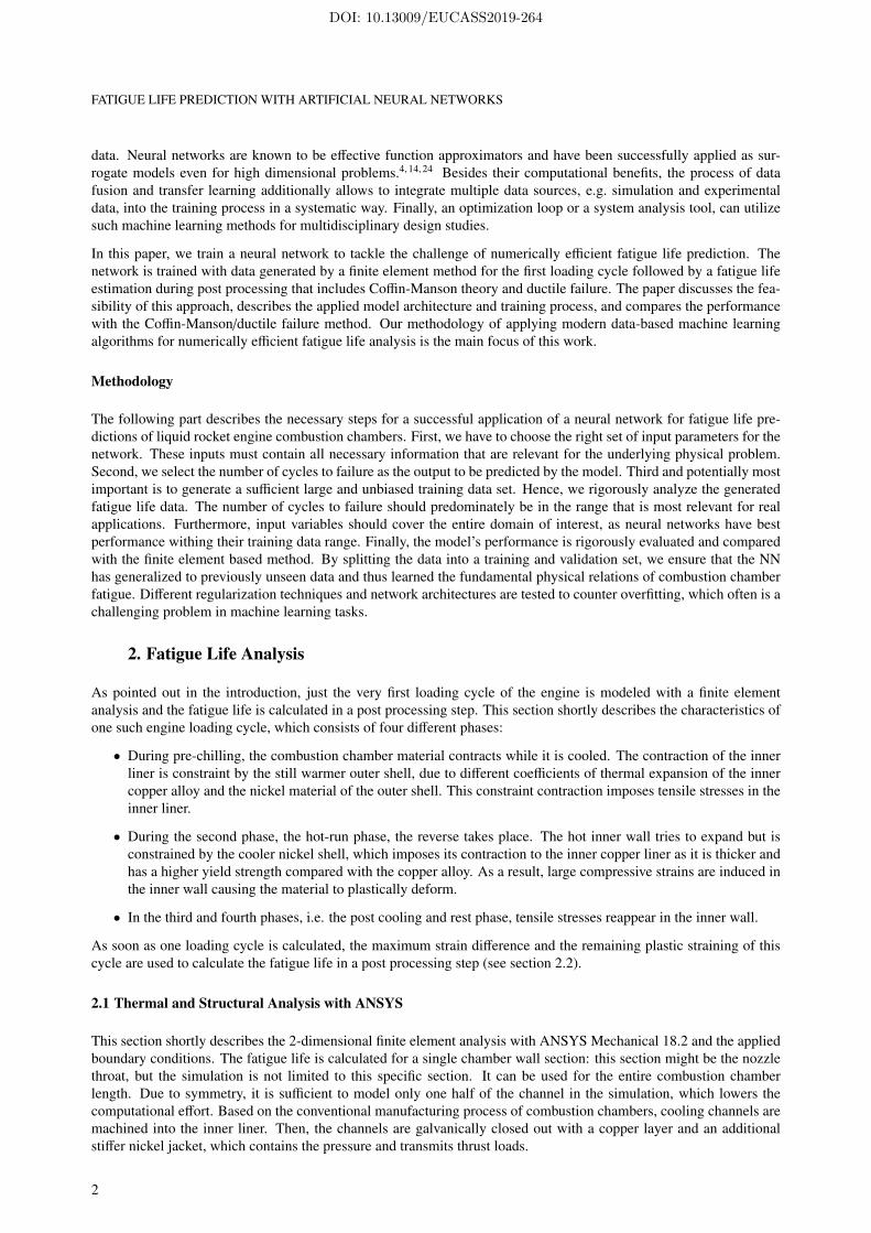
(a) Boundary conditions (b) Temperature profile during operation

Figure 1: Boundary conditions and results of the thermal analysis

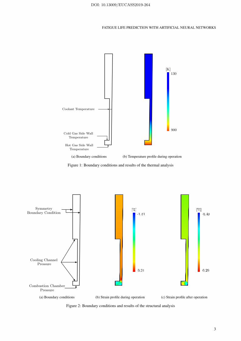
(a) Boundary conditions (b) Strain profile during operation (c) Strain profile after operation

Figure 2: Boundary conditions and results of the structural analysis

3

DOI: 10.13009/EUCASS2019-264


For thermal analysis, the outer shell temperature and the hot-gas- and cold-gas-side wall temperatures are used todetermine the temperature distribution during each of the four different engine operation phases (see figure 1b). Forsimplicity, a linear temperature decrease from the hot-gas side wall to the outer shell is assumed. Figure 1a shows thetemperature boundary conditions used for thermal analysis.

For structural analysis, the wall temperature distribution in each loading phase is applied as boundary condition. Furtherboundaries are given by the pressure difference between combustion chamber and cooling channel. The materialparameters for the inner wall, which is made from a high strengths copper alloy, were obtained from low-cycle fatigueexperiments with a strain amplitude of 2 %.3, 19 The elasto-plasticity of the wall material is modeled according to therate independent version of the Chaboche model with kinematic hardening and isotropic softening for T = 900 K andadditional isotropic hardening for T = 300 K, T = 500 K and T = 700 K. Figure 2 provides an overview of thestructural analysis. As the strain profile after operation (figure 2c) shows, plastic straining remains in the wall materialafter one loading cycle. In summary, the 2-d structural finite element analysis calculates the maximum strain differenceand the remaining plastic straining in the inner liner, which is then used in the post processing step.

2.2 Fatigue Life Prediction

The fatigue life estimation in this paper is based on the temperature depended Coffin-Manson law for low cycle fatiguewith ductile failure. The 2-d structural finite element analysis provides the minimum strain εmin, the maximum strainεmax, and the remaining strain at the end of the first cycle εend. Based on these strains, the temperature dependent numberof cycles to failure NLCF, CoffMans(∆ε,T ) is determined with the Coffin-Manson law. The fatigue usage factor u = 1/N

represents the maximum fatigue life of the material and must not exceed 1. The temperature dependent ratchetingusage factor uratch(εend, εult(T )) caused by ductile failure is defined by

uratch(εend, εult(T )) =max(0,εend)εult(T ) , (1)

with the temperature dependent ultimate strain of the chamber wall material εult(T ). In order to determine the cumula-tive usage factor utotal(T ), both partial usage factors are summed up:

utotal(T ) = 1NLCF, CoffMans(∆ε,T ) +

max(0,εend)εult(T ) . (2)

uratch considers the accumulation of tensile plastic strains during cycling loading. Finally, the total number of cycles tofailure is defined by:

NLCF, total(T ) =1

utotal(T ). (3)

By including ratcheting effects, the combustion chamber failure occurs at the symmetry line of the cooling channel.This failure mode, the so-called doghouse effect, is common in regeneratively cooled combustion chambers and hasbeen observed experimentally.18 In this phenomenon, the inner hot-gas side wall becomes thinner and finally fails bybulging out towards the interior of the combustion chamber.

3. Artificial Neural Networks

In recent years, a considerable amount of literature has been published on neural networks. The well known publicationby Goodfellow et al.6 provides an in-depth analysis of machine learning, covering both theory and practical application.It serves as basis for this chapter and is recommended for deeper insights into machine learning. This section gives ashort introduction, summarizes the theory and explains the application of neural networks to fatigue life prediction.

In general, machine learning is the capability of a system to acquire its own knowledge by extracting information andpatterns from raw data. Providing the right data to a machine learning algorithm can enable it to solve various problemssuch as image recognition or predictive analytics. Because the algorithm extracts its knowledge from the given data,it improves with more data and experience. Deep learning is a special approach to machine learning that tries to learncomplicated relationships by building them out of simpler, less complex pieces of information. A nested hierarchyof this concept brakes down complicated problems in different simpler, more abstract representations of the originalproblem. Because this concept usually results in many sequential computational layers, it is called deep learning.

4

DOI: 10.13009/EUCASS2019-264


3.1 Theory of Artificial Neural Networks

Inspired by the biological brain, deep learning methods are often referred to as artificial neural networks because ofa similar information processing.6 In general, such network consists of an input layer, multiple hidden layers and anoutput layer, which are all built out of simple elements called neurons. Each neuron receives inputs from the previouslayer, calculates the weighted sum of theses inputs according to some model parameters, and applies a nonlineartransformation to this sum to generate its output. Connections between two layers transfer the output of previousneurons to the input of the next layer. Each connection between two neurons is assigned a weight w. The strategy ofdeep learning is to learn these weights – the model parameters – so that the network can approximate some function f ∗

that represents the underlying physical problem. Among other things, neural networks can be used for regression andclassification problems.

In classification, a network separates the data into multiple categories k depending on the input vector, which meansthe algorithm is asked to output a discrete function f : Rn → {1, ...k}. Well-known examples of classification areobject recognition in images, speech recognition, or data clustering. In regression problems, the network estimates anumerical value for a given input vector with dimension n as output of the function f : Rn → R. Regression algorithmsowe their name due to their continuous output space.

3.1.1 Neuron Operation

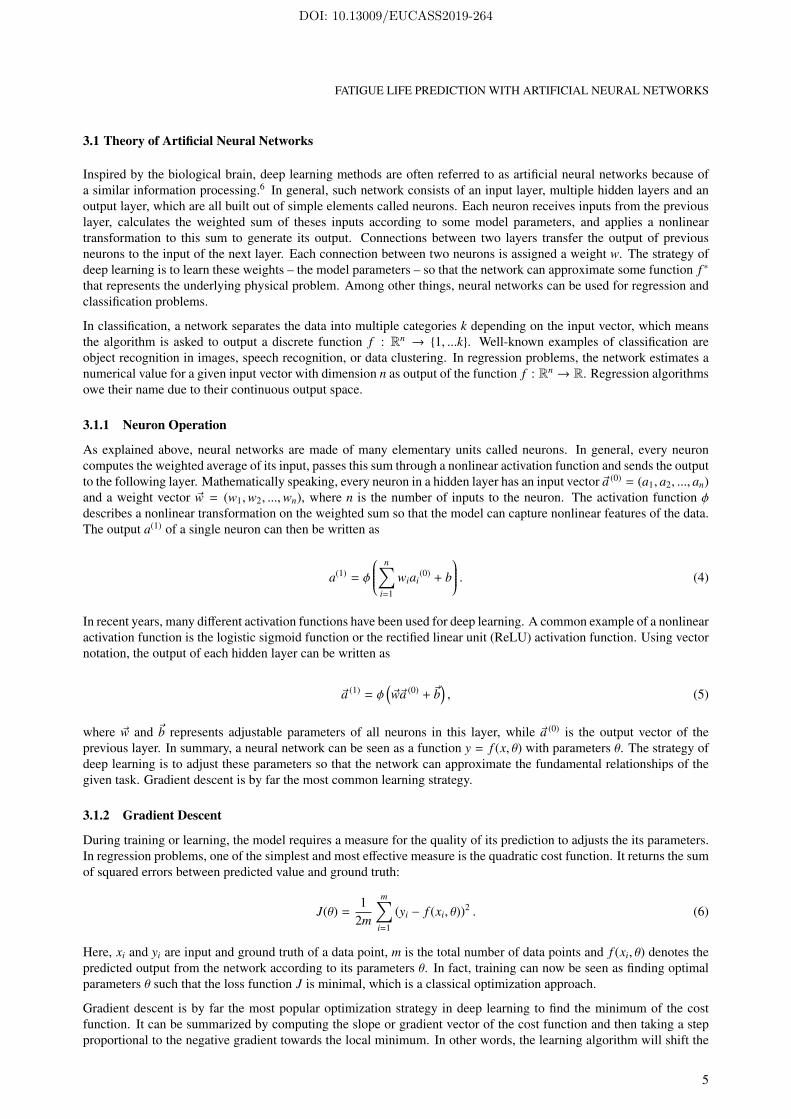
As explained above, neural networks are made of many elementary units called neurons. In general, every neuroncomputes the weighted average of its input, passes this sum through a nonlinear activation function and sends the outputto the following layer. Mathematically speaking, every neuron in a hidden layer has an input vector ~a (0) = (a1, a2, ..., an)and a weight vector ~w = (w1,w2, ...,wn), where n is the number of inputs to the neuron. The activation function φdescribes a nonlinear transformation on the weighted sum so that the model can capture nonlinear features of the data.The output a(1) of a single neuron can then be written as

a(1) = φ

n∑i=1

wiai(0) + b

. (4)

In recent years, many different activation functions have been used for deep learning. A common example of a nonlinearactivation function is the logistic sigmoid function or the rectified linear unit (ReLU) activation function. Using vectornotation, the output of each hidden layer can be written as

~a (1) = φ(~w~a (0) + ~b

), (5)

where ~w and ~b represents adjustable parameters of all neurons in this layer, while ~a (0) is the output vector of theprevious layer. In summary, a neural network can be seen as a function y = f (x, θ) with parameters θ. The strategy ofdeep learning is to adjust these parameters so that the network can approximate the fundamental relationships of thegiven task. Gradient descent is by far the most common learning strategy.

3.1.2 Gradient Descent

During training or learning, the model requires a measure for the quality of its prediction to adjusts the its parameters.In regression problems, one of the simplest and most effective measure is the quadratic cost function. It returns the sumof squared errors between predicted value and ground truth:

J(θ) =1

2m

m∑i=1

(yi − f (xi, θ))2 . (6)

Here, xi and yi are input and ground truth of a data point, m is the total number of data points and f (xi, θ) denotes thepredicted output from the network according to its parameters θ. In fact, training can now be seen as finding optimalparameters θ such that the loss function J is minimal, which is a classical optimization approach.

Gradient descent is by far the most popular optimization strategy in deep learning to find the minimum of the costfunction. It can be summarized by computing the slope or gradient vector of the cost function and then taking a stepproportional to the negative gradient towards the local minimum. In other words, the learning algorithm will shift the

5

DOI: 10.13009/EUCASS2019-264


trainable parameter of the network by a small fraction (the learning rate ε) of the computed gradient, according to thegradient vector. Mathematically speaking, gradient descent calculates a new parameter vector

~θ′ = ~θ − ε∇θJ(~θ), (7)

where ∇θJ(~θ) is the gradient of the cost function with respect to model parameters θ. However, the gradient calculationcan become computational expensive for larger data sets and a substantial network size. Thus, the gradient vector iscalculated in a more efficient way called mini-batch gradient descent. It is an variation of the classical gradient descentalgorithm that estimates the gradient on a small batch of a few hundred randomly chosen data points. This process isrepeated until the entire data have been used, which is called one epoch. Further information on gradient descent andadvanced enhancements are given in the literature.6

3.2 Generalization and Overfitting

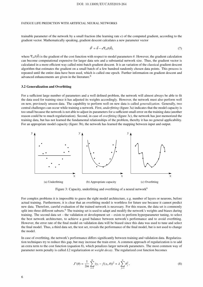
For a sufficient large number of parameters and a well defined problem, the network will almost always be able to fitthe data used for training since it has adjusted its weights accordingly. However, the network must also perform wellon new, previously unseen data. The capability to perform well on new data is called generalization. Generally, twocentral challenges can occur while training a network. First, underfitting (figure 3a) indicates that the model capacity istoo small because the network is not able to adjust its parameters for a sufficient small error on the training data (anotherreason could be to much regularization). Second, in case of overfitting (figure 3c), the network has just memorized thetraining data, but has not learned the fundamental relationships of the problem, thereby it has no general applicability.For an appropriate model capacity (figure 3b), the network has learned the mapping between input and output.

(a) Underfitting (b) Appropriate capacity (c) Overfitting

Figure 3: Capacity, underfitting and overfitting of a neural network6

For complex problems it is impossible to guess the right model architecture, e.g. number of layers or neurons, beforeactual training. Furthermore, it is clear that an overfitting model is worthless for future use because it cannot predictnew data. Therefore, careful evaluation of the trained network is necessary. For this reason, the data set is commonlysplit into three different subsets.6 The training set is used to adapt and modify the network’s weights and biases duringtraining. The second data set – the validation or development set – exists to perform hyperparameter tuning, to selectthe best network architecture, to achieve a good balance between network’s performance and to avoid overfitting.However, the error rate of the final model on validation data will be biased since this data was used to tune and selectthe final model. Thus, a third data set, the test set, reveals the performance of the final model, but is not used to changethe model.

In case of overfitting, the network’s performance differs significantly between training and validation data. Regulariza-tion techniques try to reduce this gap, but may increase the train error. A common approach of regularization is to addan extra term to the cost function (equation 8), which penalizes larger network parameters. The most common way ofparameter norm penalty is called L2 regularization or weight decay. The regularized cost function becomes

J∗(θ) =1

2m

m∑i=1

(yi − f (xi, θ))2 + λ

n∑j=1

θ2j , (8)

6

DOI: 10.13009/EUCASS2019-264


where λ is an additional hyperparameter that controls the amount of regularization and n gives the total number ofnetwork parameters. When talking about neural networks as an optimization problem, the model now tries to minimizeboth its parameters and the training error. In general, smaller model parameters prevent overfitting, thus improving gen-eralization. Additional regularization techniques, such as dropout,1, 22 early stopping16 or adding noise to models26 canfurther increase the generalization ability. Only weight decay was used for the network presented in this publication,but other techniques can be interesting for deeper networks or cases with less data.

4. Neural Network for Fatigue Life Prediction

This section presents the neural network for fatigue life prediction, describes how to find the optimal network architec-ture, discusses the training process, and analyzes the data used for training.

4.1 Data Generation

In general, a balanced and evenly distributed data set boosts the chance of successfully applying neural networks tocomplex problems. Therefore, we carefully create and analyze two separate data sets for methane and liquid hydrogen.We focus on methane, because it is the promising propellant in terms of fatigue life expectancy. Nevertheless, wesimilarly train and evaluate a second neural network for liquid hydrogen.

4.1.1 Methane Data Set

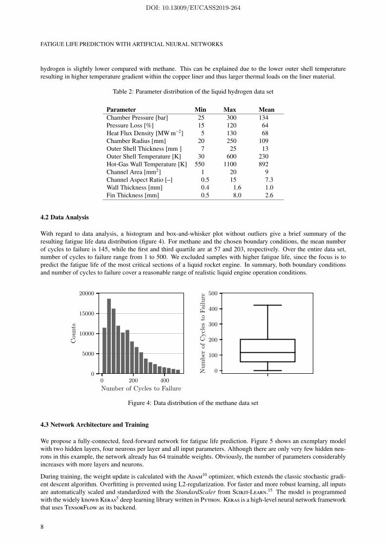
The methane data set consists of 130 000 fatigue life samples. Table 1 gives an overview of the inputs for thermaland structural analysis, and shows the minimum, maximum and mean value of each variable in the generated dataset. These lower and upper limits cover the geometrical dimensions and operation conditions of both first and upperstage liquid rocket engines and are representative for the entire combustion chamber length including the nozzle throat,which experiences the highest thermal stresses. During data generation, parameter combinations are randomly sampledwithin the given limits.

Table 1: Parameter distribution of the methane data set

Parameter Min Max MeanChamber Pressure [bar] 25 300 129Pressure Loss [%] 10 120 55Heat Flux Density [MW m−2] 5 125 64Chamber Radius [mm] 20 300 97Outer Shell Thickness [mm] 7 25 13Outer Shell Temperature [K] 110 600 286Hot-Gas Wall Temperature [K] 600 1100 900Channel Area [mm2] 1 20 9Channel Aspect Ratio [–] 0.3 15 6.2Wall Thickness [mm] 0.4 1.6 1.0Fin Thickness [mm] 0.5 8.0 2.3

Note that further variables can be easily derived. For example, heat flux density and hot-gas wall temperature determinethe cooling channel wall temperature when assuming linear one-dimensional heat conductivity in the wall material.Coolant pressure in the channel cross section is given by the combustion chamber pressure and the pressure loss:pcooling channel = (1+pressure loss) · pcombustion chamber. The fin thickness is determined by the number of cooling channelsfor a given chamber radius and channel width. The outer shell is at coolant bulk temperature, which is suitable for mostrealistic operation conditions.

4.1.2 Hydrogen Data Set

The hydrogen data set is comparable in size and variable distribution to the methane set. It consist of approximately120 000 data points, sampled from the distribution in table 2. Using liquid hydrogen at lower temperatures thanmethane, the minimal outer shell temperature is consequently lower. The resulting mean number of cycles to failureis 131, while the first and third quartile are at 46 and 191, respectively. Note that the resulting fatigue life for liquid

7

DOI: 10.13009/EUCASS2019-264


hydrogen is slightly lower compared with methane. This can be explained due to the lower outer shell temperatureresulting in higher temperature gradient within the copper liner and thus larger thermal loads on the liner material.

Table 2: Parameter distribution of the liquid hydrogen data set

Parameter Min Max MeanChamber Pressure [bar] 25 300 134Pressure Loss [%] 15 120 64Heat Flux Density [MW m−2] 5 130 68Chamber Radius [mm] 20 250 109Outer Shell Thickness [mm ] 7 25 13Outer Shell Temperature [K] 30 600 230Hot-Gas Wall Temperature [K] 550 1100 892Channel Area [mm2] 1 20 9Channel Aspect Ratio [–] 0.5 15 7.3Wall Thickness [mm] 0.4 1.6 1.0Fin Thickness [mm] 0.5 8.0 2.6

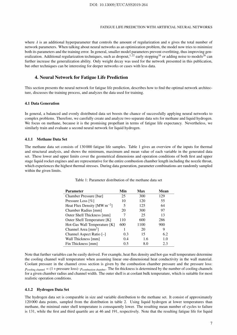
4.2 Data Analysis

With regard to data analysis, a histogram and box-and-whisker plot without outliers give a brief summary of theresulting fatigue life data distribution (figure 4). For methane and the chosen boundary conditions, the mean numberof cycles to failure is 145, while the first and third quartile are at 57 and 203, respectively. Over the entire data set,number of cycles to failure range from 1 to 500. We excluded samples with higher fatigue life, since the focus is topredict the fatigue life of the most critical sections of a liquid rocket engine. In summary, both boundary conditionsand number of cycles to failure cover a reasonable range of realistic liquid engine operation conditions.

0 200 400

Number of Cycles to Failure

0

5000

10000

15000

20000

Cou

nts

T

Number of Cycles to Failure

0

100

200

300

400

500

Nu

mb

erof

Cycl

esto

Fai

lure

Figure 4: Data distribution of the methane data set

4.3 Network Architecture and Training

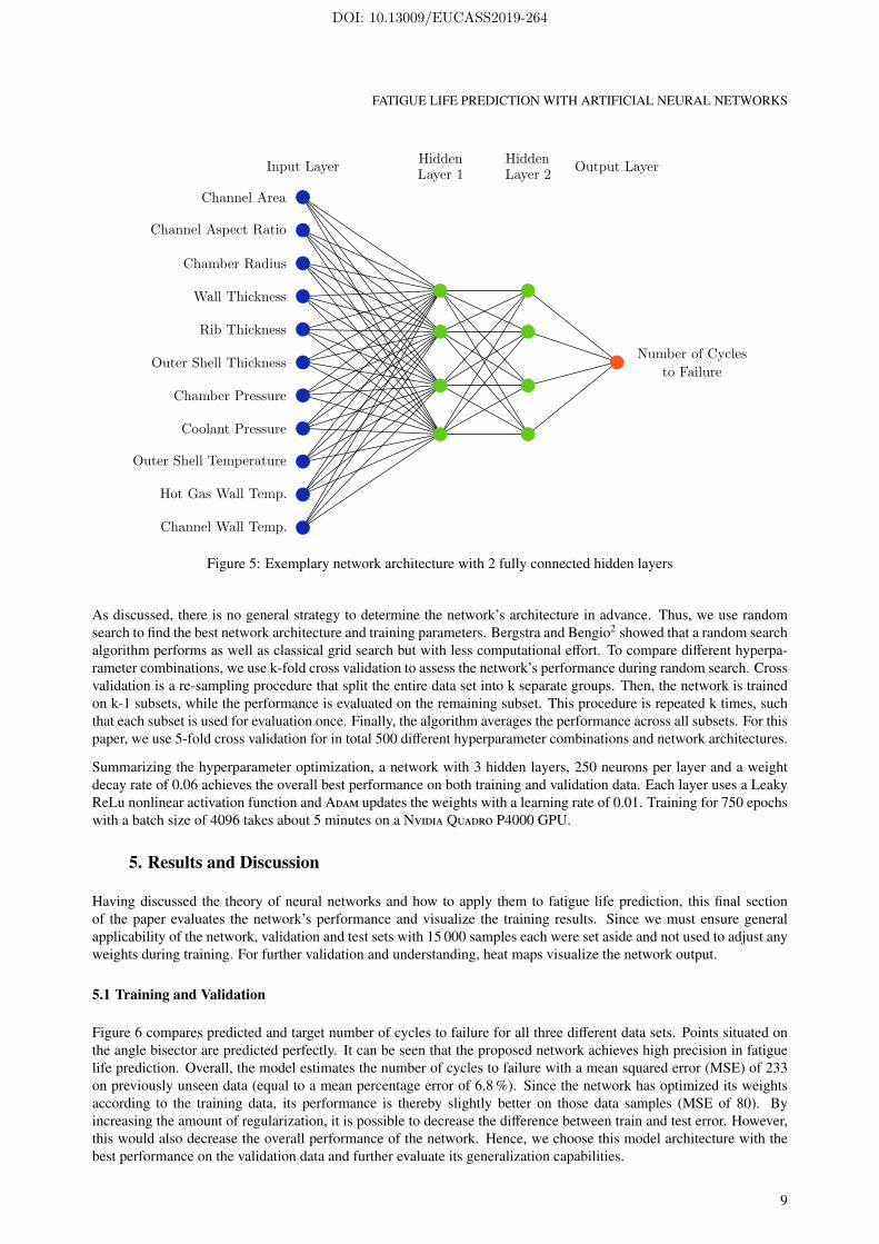
We propose a fully-connected, feed-forward network for fatigue life prediction. Figure 5 shows an exemplary modelwith two hidden layers, four neurons per layer and all input parameters. Although there are only very few hidden neu-rons in this example, the network already has 64 trainable weights. Obviously, the number of parameters considerablyincreases with more layers and neurons.

During training, the weight update is calculated with the Adam10 optimizer, which extends the classic stochastic gradi-ent descent algorithm. Overfitting is prevented using L2-regularization. For faster and more robust learning, all inputsare automatically scaled and standardized with the StandardScaler from Scikit-Learn.15 The model is programmedwith the widely known Keras5 deep learning library written in Python. Keras is a high-level neural network frameworkthat uses TensorFlow as its backend.

8

DOI: 10.13009/EUCASS2019-264


Figure 5: Exemplary network architecture with 2 fully connected hidden layers

As discussed, there is no general strategy to determine the network’s architecture in advance. Thus, we use randomsearch to find the best network architecture and training parameters. Bergstra and Bengio2 showed that a random searchalgorithm performs as well as classical grid search but with less computational effort. To compare different hyperpa-rameter combinations, we use k-fold cross validation to assess the network’s performance during random search. Crossvalidation is a re-sampling procedure that split the entire data set into k separate groups. Then, the network is trainedon k-1 subsets, while the performance is evaluated on the remaining subset. This procedure is repeated k times, suchthat each subset is used for evaluation once. Finally, the algorithm averages the performance across all subsets. For thispaper, we use 5-fold cross validation for in total 500 different hyperparameter combinations and network architectures.

Summarizing the hyperparameter optimization, a network with 3 hidden layers, 250 neurons per layer and a weightdecay rate of 0.06 achieves the overall best performance on both training and validation data. Each layer uses a LeakyReLu nonlinear activation function and Adam updates the weights with a learning rate of 0.01. Training for 750 epochswith a batch size of 4096 takes about 5 minutes on a Nvidia Quadro P4000 GPU.

5. Results and Discussion

Having discussed the theory of neural networks and how to apply them to fatigue life prediction, this final sectionof the paper evaluates the network’s performance and visualize the training results. Since we must ensure generalapplicability of the network, validation and test sets with 15 000 samples each were set aside and not used to adjust anyweights during training. For further validation and understanding, heat maps visualize the network output.

5.1 Training and Validation

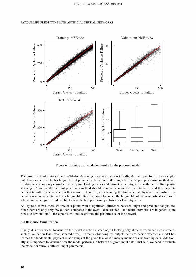
Figure 6 compares predicted and target number of cycles to failure for all three different data sets. Points situated onthe angle bisector are predicted perfectly. It can be seen that the proposed network achieves high precision in fatiguelife prediction. Overall, the model estimates the number of cycles to failure with a mean squared error (MSE) of 233on previously unseen data (equal to a mean percentage error of 6.8 %). Since the network has optimized its weightsaccording to the training data, its performance is thereby slightly better on those data samples (MSE of 80). Byincreasing the amount of regularization, it is possible to decrease the difference between train and test error. However,this would also decrease the overall performance of the network. Hence, we choose this model architecture with thebest performance on the validation data and further evaluate its generalization capabilities.

9

DOI: 10.13009/EUCASS2019-264


0 250 500

Target Cycles to Failure

0

250

500

Pre

dic

ted

Cycl

esto

Failu

reTraining: MSE=80

0 250 500


0

250

500

Pre

dic

ted

Cycl

esto

Failu

re

Validation: MSE=233

0 250 500


0

250

500

Pre

dic

ted

Cycl

esto

Fai

lure

Test: MSE=239

Train Validation Test

Delta Cycles to Failure

0

5

10

15

Del

taC

ycl

esto

Fai

lure

Figure 6: Training and validation results for the proposed model

The error distribution for test and validation data suggests that the network is slightly more precise for data sampleswith lower rather than higher fatigue life. A possible explanation for this might be that the post processing method usedfor data generation only considers the very first loading cycles and estimates the fatigue life with the resulting plasticstraining. Consequently, the post processing method should be more accurate for low fatigue life and thus generatebetter data with lower variance in this region. Therefore, after learning the fundamental physical relationships, thenetwork is more accurate for lower fatigue life. Since we want to predict the fatigue life of the most critical sections ofa liquid rocket engine, it is desirable to have the best performing network for low fatigue life.

As Figure 6 shows, there are few data points with a significant difference between target and predicted fatigue life.Since there are only very few outliers compared to the overall data set size – and neural networks are in general quiterobust to few outliers8 – these points will not deteriorate the performance of the network.

5.2 Response Visualization

Finally, it is often useful to visualize the model in action instead of just looking only at the performance measurementssuch as validation loss (mean-squared-error). Directly observing the outputs helps to decide whether a model haslearned the fundamental physical relationships of the given task or if it merely memorizes the training data. Addition-ally, it is important to visualize how the model performs in between of given input data. That said, we need to evaluatethe model for various different input parameters.

10

DOI: 10.13009/EUCASS2019-264


Heat Map

A heat map is a visualization technique that shows the model’s answer to given inputs. In other words, it can bedescribed as a parametric study in which two inputs change while all other parameters are kept the same. The output,i.e. the number of cycles to failure, is then plotted in a two-dimensional scatter plot, where both free inputs are usedas x- and y-axis. The analysis of this heat map can identify possible problems in terms of overfitting. For example,further investigations would be necessary for regions with strong discontinuities or peaks in fatigue life where we donot expect such peaks from our physical understanding.

700 800 900 1000 1100

Hot-Gas Wall Temperature [K]

25

50

75

100

125

150

175

200

∆T

[K]

700 800 900 1000 1100


0.4

0.6

0.8

1.0

Pre

ssure

Loss

[−]

50

100

150

200

250

300

350

Num

ber

of

Cycl

esto

Failure

(a) Hot-gas wall temperature and ∆T (b) Hot-gas wall temperature and pressure loss

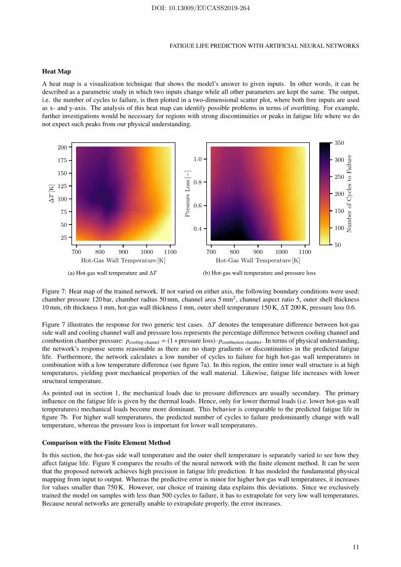
Figure 7: Heat map of the trained network. If not varied on either axis, the following boundary conditions were used:chamber pressure 120 bar, chamber radius 50 mm, channel area 5 mm2, channel aspect ratio 5, outer shell thickness10 mm, rib thickness 1 mm, hot-gas wall thickness 1 mm, outer shell temperature 150 K, ∆T 200 K, pressure loss 0.6.

Figure 7 illustrates the response for two generic test cases. ∆T denotes the temperature difference between hot-gasside wall and cooling channel wall and pressure loss represents the percentage difference between cooling channel andcombustion chamber pressure: pcooling channel = (1+pressure loss) · pcombustion chamber. In terms of physical understanding,the network’s response seems reasonable as there are no sharp gradients or discontinuities in the predicted fatiguelife. Furthermore, the network calculates a low number of cycles to failure for high hot-gas wall temperatures incombination with a low temperature difference (see figure 7a). In this region, the entire inner wall structure is at hightemperatures, yielding poor mechanical properties of the wall material. Likewise, fatigue life increases with lowerstructural temperature.

As pointed out in section 1, the mechanical loads due to pressure differences are usually secondary. The primaryinfluence on the fatigue life is given by the thermal loads. Hence, only for lower thermal loads (i.e. lower hot-gas walltemperatures) mechanical loads become more dominant. This behavior is comparable to the predicted fatigue life infigure 7b. For higher wall temperatures, the predicted number of cycles to failure predominantly change with walltemperature, whereas the pressure loss is important for lower wall temperatures.

Comparison with the Finite Element Method

In this section, the hot-gas side wall temperature and the outer shell temperature is separately varied to see how theyaffect fatigue life. Figure 8 compares the results of the neural network with the finite element method. It can be seenthat the proposed network achieves high precision in fatigue life prediction. It has modeled the fundamental physicalmapping from input to output. Whereas the predictive error is minor for higher hot-gas wall temperatures, it increasesfor values smaller than 750 K. However, our choice of training data explains this deviations. Since we exclusivelytrained the model on samples with less than 500 cycles to failure, it has to extrapolate for very low wall temperatures.Because neural networks are generally unable to extrapolate properly, the error increases.

11

DOI: 10.13009/EUCASS2019-264


700 800 900 1000 1100


0

200

400

600

800N

um

ber

of

Cycl

esto

Fail

ure Ansys

NN

100 200 300 400 500

Outer Shell Temperature [K]

100

150

200

250

300

Nu

mb

erof

Cycl

esto

Fail

ure Ansys

NN

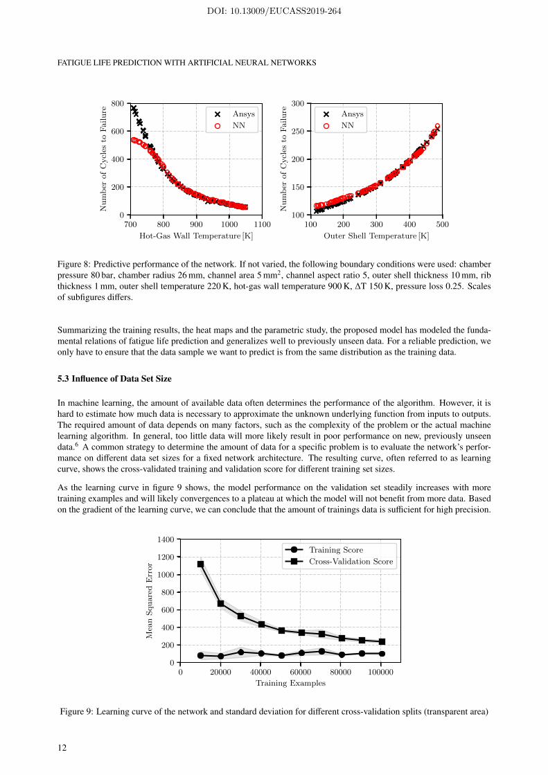
Figure 8: Predictive performance of the network. If not varied, the following boundary conditions were used: chamberpressure 80 bar, chamber radius 26 mm, channel area 5 mm2, channel aspect ratio 5, outer shell thickness 10 mm, ribthickness 1 mm, outer shell temperature 220 K, hot-gas wall temperature 900 K, ∆T 150 K, pressure loss 0.25. Scalesof subfigures differs.

Summarizing the training results, the heat maps and the parametric study, the proposed model has modeled the funda-mental relations of fatigue life prediction and generalizes well to previously unseen data. For a reliable prediction, weonly have to ensure that the data sample we want to predict is from the same distribution as the training data.

5.3 Influence of Data Set Size

In machine learning, the amount of available data often determines the performance of the algorithm. However, it ishard to estimate how much data is necessary to approximate the unknown underlying function from inputs to outputs.The required amount of data depends on many factors, such as the complexity of the problem or the actual machinelearning algorithm. In general, too little data will more likely result in poor performance on new, previously unseendata.6 A common strategy to determine the amount of data for a specific problem is to evaluate the network’s perfor-mance on different data set sizes for a fixed network architecture. The resulting curve, often referred to as learningcurve, shows the cross-validated training and validation score for different training set sizes.

As the learning curve in figure 9 shows, the model performance on the validation set steadily increases with moretraining examples and will likely convergences to a plateau at which the model will not benefit from more data. Basedon the gradient of the learning curve, we can conclude that the amount of trainings data is sufficient for high precision.

0 20000 40000 60000 80000 100000

Training Examples

0

200

400

600

800

1000

1200

1400

Mea

nSquare

dE

rror

Training Score

Cross-Validation Score

Figure 9: Learning curve of the network and standard deviation for different cross-validation splits (transparent area)

12

DOI: 10.13009/EUCASS2019-264


5.4 Hydrogen Data Set

Using the same architecture and validation process (section 2.2 and chapter 5), we trained a second model for liquidhydrogen. The model fits the data with a mean squared error of 93, 264 and 290 on validation, training and testdata, respectively. These results correspond to a mean absolute percentage error of 7.2 % on previously unseen data.Summarizing the validation, we can conclude that a neural network performs equally as well for liquid hydrogen as itdoes for methane.

5.5 Performance measurement

The overall goal of this research was to develop a numerically efficient method for fatigue life prediction of liquidrocket engine combustion chambers. Although neural networks require a time-intensive learning phase and a largeamount of training data, their predictive speed is high because the network only has to multiply the input vector withits weight matrices to generate the output. Additionally, the numerical effort does not depended on the actual valueof the inputs (e.g. size of the combustion chamber), whereas finite element based methods do need increasingly moretime with larger model sizes and thus higher number of mesh elements.

On a computer with an Intel XeonW-2123 CPU, fatigue life analysis with AnsysMechanical takes approximately 2to 5 minutes depending on the model size. In contrast, the neural network computes 1 000 000 data samples in 12 son the same CPU, which is an average of 12 µs per calculation. This comparison shows the great potential of suchdata-driven methods for multidisciplinary design studies or optimization loops.

6. Summary and Outlook

In this paper, an artificial neural network was successfully trained to predict the fatigue life of liquid rocket enginecombustion chambers. The network was trained on data generated by a finite element method for the first loadingcycles combined with a post processing approach to estimate the number of cycles to failure. This approach combinesthe Coffin-Manson method for low cycle fatigue with ductile failure caused by ratcheting effects during post processing.After training, the proposed neural network predicts previously unseen data with a mean absolute percentage error of6.8 % and 7.2 % for methane and liquid hydrogen, respectively. Hence, we can conclude that it has closely modeledthe underlying relations of fatigue in rocket engine combustion chambers.

In summary, the results have proven the feasibility of applying modern data-based machine learning algorithms fornumerically efficient fatigue life estimation. By splitting the data into different subsets for training, validation andtesting, we demonstrated the general applicability of the network. Moreover, the proposed network predicts the num-ber of cycles to failure in under 0.1 ms, which is up to 107 times faster than classical finite element based methods.Due to this enormous time benefit, a data-based algorithm is well suited to be embedded in a system analysis tool,e.g. EcosimPro/ESPSS. Thus, this numerically efficient method facilitates more sophisticated, multidisciplinary designstudies that could optimize an entire engine cycle for maximum fatigue life. Furthermore, the neural network could beused in the design phase of a new engine to optimize the cooling channel geometry or the operating conditions of theengine.

However, modern data-based algorithms (like neural networks) also have natural drawbacks. Due to the high numberof parameters, these algorithms often lack a deeper understanding of the fundamental physics. Furthermore, neuralnetworks cannot extrapolate, but only provide reliable and robust predictions within the training subspace. In summary,domain knowledge and the understanding of physical processes will always be crucially important to evaluate andjustify the prediction of data-driven algorithms.

Further research could investigate the process of data fusion and transfer learning that allows to integrate multipledata sources into the training, e.g. experimental data. This approach could further improve the network’s performance.Using the proposed network, future investigations can analyze fatigue life expectancies for different propellant com-binations, operating conditions, or various combustion chamber geometries in the context of reusability. This work isthe first time an artificial neural network was trained for fatigue life predictions (to the best of our knowledge). It willhopefully serve as a base for future studies on optimizing an entire engine design for maximum fatigue life.

7. Acknowledgments

It is a pleasure to thank R. Dos Santos Hahn and C. Schorn for comments that greatly improved this paper.

13

DOI: 10.13009/EUCASS2019-264


References

[1] P. Baldi and P. Sadowski. Understanding dropout. In Advances in Neural Information Processing Systems 26.Curran Associates, Inc., 2013.

[2] J. Bergstra and Y. Bengio. Random search for hyper-parameter optimization. Journal of Machine LearningResearch, 2012.

[3] W. Bouajila and J. Riccius. Identification of the unified chaboche constitutive model’s parameters for a costefficient copper-based alloy. Space Propulsion. Cologne, Germany, 2014.

[4] W. Chang, X. Chu, A. Fareed, S. Pandey, J. Luo, B. Weigand, and E. Laurien. Heat transfer prediction ofsupercritical water with artificial neural networks. Applied Thermal Engineering, 2018.

[5] F. Chollet et al. Keras, 2015.

[6] I. Goodfellow, Y. Bengio, and A. Courville. Deep Learning. The MIT Press, 2017.

[7] A. Iannetti. Prometheus, a lox/lch4 reusable rocket engine. Proceedings of the 7th European Conference forAeronautics and Space Sciences. Milano, Italy, 2017.

[8] A. Khamis. The effects of outliers data on neural network performance. Journal of Applied Sciences, 2001.

[9] T. Kimura, T. Hashimoto, M. Sato, S. Takada, S. Moriya, T. Yagishita, Y. Naruo, H. Ogawa, T. Ito, K. Obase,and H. Ohmura. Reusable rocket engine: Firing tests and lifetime analysis of combustion chamber. Journal ofPropulsion and Power, 2016.

[10] D. Kingma and J. Ba. Adam: A method for stochastic optimization. International Conference on LearningRepresentations. Banff, Canada, 2014.

[11] D.E. Koelle. Handbook of Cost Engineering and Design of Space Transportation Systems. TCS - TransCostSys-tems, 2013.

[12] D. Kuhl, J. Riccius, and O. Haidn. Thermomechanical analysis and optimization of cryogenic liquid rocketengines. Journal of Propulsion and Power, 2002.

[13] T. Masuoka and J. Riccius. Life evaluation of a combustion chamber by thermomechanical fatigue panel testsbased on a creep fatigue and ductile damage model. International Journal of Damage Mechanics, 2019.

[14] O. Ogunmolu, X. Gu, S. B. Jiang, and N. R. Gans. Nonlinear systems identification using deep dynamic neuralnetworks. CoRR, 2016.

[15] F. Pedregosa, G. Varoquaux, A. Gramfort, V. Michel, B. Thirion, O. Grisel, M. Blondel, P. Prettenhofer, R. Weiss,V. Dubourg, J. Vanderplas, A. Passos, D. Cournapeau, M. Brucher, M. Perrot, and E. Duchesnay. Scikit-learn:Machine learning in Python. Journal of Machine Learning Research, 2011.

[16] L. Prechelt. Neural Networks: Tricks of the Trade: Second Edition, chapter Early Stopping — But When?Springer, 2012.

[17] R Quentmeyer. Experimental fatigue life investigation of cylindrical thrust chambers. 13th Propulsion Confer-ence. Orlando, FL, 1977.

[18] J. Riccius and E. Zametaev. Stationary and dynamic thermal analyses of cryogenic liquid rocket combustionchamber walls. AIAA/ASME/SAE/ASEE Joint Propulsion Conference and Exhibit, Indianapolis, IN, 2002.

[19] J. Riccius, E. Zametaev, W. Bouajila, and Q. Wargnier. Inner liner temperature variation caused deformation lo-calization effects in a multichannel model of a generic lre wall structure. AIAA Propulsion and Energy, Cleveland,OH, 2014.

[20] M. Rudis and J. Riccius. Liquid rocket engine component failure probability and residual life prediction atthermal and mechanical cyclic loading. 4th European Congress on Computational Methods in Applied Sciencesand Engineering, ECCOMAS, Jyväskylä, Finland, 2004.

[21] W. Schwarz, S. Schwub, K. Quering, D. Wiedmann, H. W. Höppel, and M. Göken. Life prediction of thermallyhighly loaded components: modelling the damage process of a rocket combustion chamber hot wall. CEAS SpaceJournal, 2011.

14

DOI: 10.13009/EUCASS2019-264


[22] N. Srivastava, G. Hinton, A. Krizhevsky, I. Sutskever, and R. Salakhutdinov. Dropout: A simple way to preventneural networks from overfitting. Journal of Machine Learning Research, 2014.

[23] G. Thiede, E. Zametaev, J. Riccius, and S. Reese. Comparison of damage parameter based finite element fatiguelife analysis results to combustion chamber type TMF panel test results. 51st AIAA/SAE/ASEE Joint PropulsionConference, Orlando, FL, 2015.

[24] G. Waxenegger-Wilfing, K. Dresia, J. Deeken, and M. Oschwald. Heat transfer prediction for supercriticalmethane flowing in rocket engine cooling channels with artificial neural networks. In Preperation.

[25] G. Waxenegger-Wilfing, J. Riccius, E. Zametaev, J. Deeken, and J. Sand. Implications of cycle variants, pro-pellant combinations and operating regimes on fatigue life expectancies of liquid rocket engines. 7th EuropeanConference for Aero-Space Sciences, Milan, Italy, 2017.

[26] R. Zur, Y. Jiang, L. L. Pesce, and K. Drukker. Noise injection for training artificial neural networks: A comparisonwith weight decay and early stopping. Medical Physics, 2009.

15

DOI: 10.13009/EUCASS2019-264

Documents

Numerically E cient Fatigue Life Prediction of Rocket