Numericalmethodsforporousmetalswith deformation … · · 2005-09-29deformation. The numerical implementation of the anisotropic elastic–plastic model in a ﬁnite element programandanalgorithmforthenumericalintegrationoftheelastoplasticequationsarepresented.The

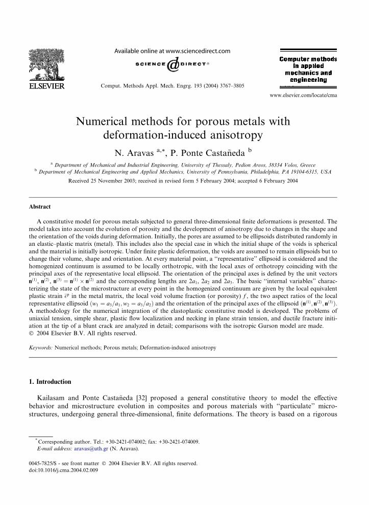
Comput. Methods Appl. Mech. Engrg. 193 (2004) 3767–3805

www.elsevier.com/locate/cma

Numerical methods for porous metals withdeformation-induced anisotropy

N. Aravas a,*, P. Ponte Casta~neda b

a Department of Mechanical and Industrial Engineering, University of Thessaly, Pedion Areos, 38334 Volos, Greeceb Department of Mechanical Engineering and Applied Mechanics, University of Pennsylvania, Philadelphia, PA 19104-6315, USA

Received 25 November 2003; received in revised form 5 February 2004; accepted 6 February 2004

Abstract

A constitutive model for porous metals subjected to general three-dimensional finite deformations is presented. The

model takes into account the evolution of porosity and the development of anisotropy due to changes in the shape and

the orientation of the voids during deformation. Initially, the pores are assumed to be ellipsoids distributed randomly in

an elastic–plastic matrix (metal). This includes also the special case in which the initial shape of the voids is spherical

and the material is initially isotropic. Under finite plastic deformation, the voids are assumed to remain ellipsoids but to

change their volume, shape and orientation. At every material point, a ‘‘representative’’ ellipsoid is considered and the

homogenized continuum is assumed to be locally orthotropic, with the local axes of orthotropy coinciding with the

principal axes of the representative local ellipsoid. The orientation of the principal axes is defined by the unit vectors

nð1Þ, nð2Þ, nð3Þ ¼ nð1Þ � nð2Þ and the corresponding lengths are 2a1, 2a2 and 2a3. The basic ‘‘internal variables’’ charac-

terizing the state of the microstructure at every point in the homogenized continuum are given by the local equivalent

plastic strain ��p in the metal matrix, the local void volume fraction (or porosity) f , the two aspect ratios of the local

representative ellipsoid ðw1 ¼ a3=a1;w2 ¼ a3=a2Þ and the orientation of the principal axes of the ellipsoid ðnð1Þ; nð2Þ; nð3ÞÞ.A methodology for the numerical integration of the elastoplastic constitutive model is developed. The problems of

uniaxial tension, simple shear, plastic flow localization and necking in plane strain tension, and ductile fracture initi-

ation at the tip of a blunt crack are analyzed in detail; comparisons with the isotropic Gurson model are made.

� 2004 Elsevier B.V. All rights reserved.

Keywords: Numerical methods; Porous metals; Deformation-induced anisotropy

1. Introduction

Kailasam and Ponte Casta~neda [32] proposed a general constitutive theory to model the effective

behavior and microstructure evolution in composites and porous materials with ‘‘particulate’’ micro-structures, undergoing general three-dimensional, finite deformations. The theory is based on a rigorous

* Corresponding author. Tel.: +30-2421-074002; fax: +30-2421-074009.

E-mail address: [email protected] (N. Aravas).

0045-7825/$ - see front matter � 2004 Elsevier B.V. All rights reserved.

doi:10.1016/j.cma.2004.02.009

mail to: [email protected]

3768 N. Aravas, P. Ponte Casta~neda / Comput. Methods Appl. Mech. Engrg. 193 (2004) 3767–3805

homogenization technique [46] and builds on earlier work [31,33,34,48,49]. It is applicable to heterogeneousmaterials consisting of randomly oriented and distributed ellipsoidal inclusions (or pores), which, in the

most general case, can change their size, shape and orientation, as a consequence of the applied defor-

mation. In addition, the ‘‘shape’’ and ‘‘orientation’’ of the center-to-center statistical distribution functions

of the inclusions [47] can also evolve with the deformation. The special case of porous metals was con-

sidered in some detail by Kailasam and Ponte Casta~neda [31] and Kailasam et al. [34,35]. For these

materials, it was found [34] that the ‘‘distribution’’ effects were small, and it was observed that the

approximation of fixing the evolution of the shape and orientation of the distribution function equal to that

of the voids themselves had a small overall effect in the predictions, while greatly simplifying the calcula-tions involved (especially for situations where the distribution ellipsoid and inclusions are not aligned). In

this work, use will be made of this simplifying assumption––keeping in mind that it could easily be relaxed

at the expense of slightly heavier computation times. In addition, all the voids will be taken here to have

initially the same shape and orientation, even if the general theory [32] can be used to treat the more general

case of several families of aligned pores (with different shape and orientation for each family). In particular,

the general theory would allow treatment of the case of randomly oriented voids, but this would result in

considerable increase in the number of internal variables required, somewhat analogous to the situtation for

polycrystals, for which a version of the theory has also been developed recently [16].Thus, the pores will be assumed in this work to be initially ellipsoidal (all with identical shapes and

orientations) and distributed randomly (with the same shape and orientation for the distribution as for the

voids themselves) in an elastic–plastic matrix (metal). Under finite plastic deformation, the voids remain

ellipsoidal but change their volume, shape and orientation with the ‘‘local’’ macroscopic deformation. In

this connection, it is emphasized that the size of the voids is assumed to be much smaller than the scale of

variation of the macroscopic fields, in such a way that any ‘‘representative volume element’’ of the porous

metal deforms uniformly with the local fields. It then makes sense to introduce, at each point in the

homogenized continuum, a ‘‘representative’’ ellipsoid with principal axes defined by the unit vectors nð1Þ,nð2Þ, nð3Þ ¼ nð1Þ � nð2Þ and corresponding principal lengths a1, a2, and a3. The homogenized continuum is

locally orthotropic, with the local axes of orthotropy coinciding with the principal axes of the representative

ellipsoid. The basic ‘‘internal variables’’ characterizing the state of the microstructure at every point in the

homogenized continuum are the equivalent plastic strain in the matrix ð��pÞ, the local void volume fraction

or porosity ðf Þ, the two aspect ratios of the local representative ellipsoid (w1 ¼ a3=a1 and w2 ¼ a3=a2), andthe orientation of the principal axes of the ellipsoid ðnð1Þ; nð2Þ; nð3ÞÞ. The yield function of the homogenized

continuum depends on the stress tensor and the aforementioned state variables; the ‘‘associated’’ plastic

flow rule is derived from the yield function by using the ‘‘normality’’ rule. The plastic model is completed bythe evolution equations of the state variables. A distinguishing feature of the model is that the rotation of

the local axes of orthotropy during plastic flow is properly accounted for.

Several aspects of the aforementioned homogenization problem have been considered also by Gologanu

et al. [17,18] and G�ar�ajeu et al. [12,13]. In particular, constitutive equations for axisymmetric loading of

porous metals with a perfectly-plastic matrix containing axisymmetric ellipsoidal cavities have been

developed by Gologanu et al. [17,18], who carried out ‘‘upper bound’’ calculations by using kinematically

admissible velocity fields. The same problem for a viscoplastic matrix has been considered by G�ar�ajeu et al.

[12,13], who derived expressions for the effective ‘‘dissipation potential’’ by using kinematically admissiblevelocity fields. It should be emphasized that a limitation of these models is that the voids were loaded

axisymmetrically, so that their orientation was assumed to remain fixed.

In the present paper we focus on the computational issues associated with the use of the constitutive

model of Kailasam and Ponte Casta~neda [31,32] for porous metals in problems involving finite plastic

deformation. The numerical implementation of the anisotropic elastic–plastic model in a finite element

program and an algorithm for the numerical integration of the elastoplastic equations are presented. The

problems of uniaxial tension, simple shear, plastic flow localization and necking in plane strain tension, and

N. Aravas, P. Ponte Casta~neda / Comput. Methods Appl. Mech. Engrg. 193 (2004) 3767–3805 3769

ductile fracture initiation at the tip of a blunt crack are analyzed in detail. Comparisons with the isotropicGurson model in which the voids are assumed to remain spherical during plastic flow are made.

Standard notation is used throughout. Boldface symbols denote tensors the orders of which are indi-

cated by the context. All tensor components are written with respect to a fixed Cartesian coordinate system

with base vectors ei, ði ¼ 1; 2; 3Þ, and the summation convention is used for repeated Latin indices, unless

otherwise indicated. The prefixes tr and det indicate the trace and the determinant, respectively, a super-

script ‘T’ the transpose, a superposed dot the material time derivative, and the subscripts ‘s’ and ‘a’ the

symmetric and anti-symmetric parts of a second-order tensor. Let a, b, c, d be vectors, A, B second-order

tensors, and C, D fourth-order tensors; the following products are used in the text a � b ¼ aibi, ðabÞij ¼ aibj,ðabcdÞijkl ¼ aibjckdl, ðA � aÞi ¼ Aikak, ða � AÞi ¼ akAki, A : B ¼ AijBij, ðA � BÞij ¼ AikBkj, ðABÞijkl ¼ AijBkl,a � A � b ¼ aiAijbj ¼ ðabÞ : A, ðC : AÞij ¼ CijklAkl, ðA : CÞij ¼ AklCklij, A : C : B ¼ AijCijklBkl and ðC : DÞijkl ¼CijpqDpqkl. The inverse C

�1 of a fourth-order tensor C that has the ‘‘minor’’ symmetries Cijkl ¼ Cjikl ¼ Cijlk isdefined so that C : C�1 ¼ C�1 : C ¼ I, where I is the symmetric fourth-order identity tensor with Cartesian

components Iijkl ¼ ðdikdjl þ dildjkÞ=2, dij being the Kronecker delta.

2. Description of the constitutive model

In this section, the anisotropic elastic–plastic constitutive model for porous metals is described. The voids

are assumed to be initially ellipsoidal and uniformly distributed in the isotropic metal matrix; as a con-sequence the porous metal is initially locally orthotropic. When the porous material is subjected to finite

plastic deformations, the voids are assumed to remain ellipsoidal, but to change their volume and shape.

This includes also the special case in which the initial shape of the voids is spherical and the material is

initially isotropic. At every point in the homogenized porous metal a ‘‘representative local ellipsoid’’ is

defined. Let ðnð1Þ; nð2Þ; nð3Þ ¼ nð1Þ � nð2ÞÞ be unit vectors in the directions of the principal axes of the local

ellipsoid and ð2a1; 2a2; 2a3Þ the corresponding lengths of the principal axes. The aspect ratios of the local

ellipsoid are defined as ðw1 ¼ a3=a1;w2 ¼ a3=a2Þ. For simplicity and because spatial distributions effects are

not expected to be significant for porous materials, the assumption is made, within the context the estimatesof Ponte Casta~neda and Willis [47], that the ‘‘shape’’ and ‘‘orientation’’ of the two-point correlation

function characterizing the distribution of the voids in space has the same shape and orientation as the

voids themselves. Then, it can be assumed that, as the material deforms, both the voids and their distri-

bution evolve with identical shapes and orientations. This allows the use of the simplified linear-elastic

estimates of Willis [53,54], as was done by Ponte Casta~neda and Zaidman [48] in their original treatment of

microstructure evolution in porous metals. In particular, this means that the porous material develops and

maintains locally orthotropic symmetry; the local axes of orthotropy are aligned with the axes of the local

representative ellipsoid. The ‘‘internal variables’’ that characterize the local state of the homogenizedporous metal are s ¼ f��p; f ;w1;w2; n

ð1Þ; nð2Þ; nð3Þg, where ��p is the local equivalent plastic strain in the metal

matrix, and f the local void-volume-fraction or porosity.

The elastic and plastic response of the porous materials are treated independently, and combined later to

obtain the full elastic–plastic response. The rate-of-deformation tensor D at every point in the homogenized

porous material is written as

D ¼ De þDp; ð1Þ

where De and Dp are the elastic and plastic parts.

The constitutive model is presented next in three parts. The first part 2.1 deals with the elastic response of

the porous metal. The yield condition and the plastic flow rule are presented in the second part 2.2. The

third part 2.3 is concerned with evolution laws for the internal variables. Finally, in part 2.4 the elastic and


plastic constitutive equations are combined in order to derive the rate form of the elastoplastic equations,which relate the rate of deformation D to the Jaumman derivative r

rof the Cauchy (true) stress tensor r.

2.1. Elastic constitutive relations

A hypoelastic form is assumed for the elastic part of the rate-of-deformation tensor:

De ¼ M e : r�; ð2Þ

where M e is the effective elastic compliance tensor and r�is a rate of the Cauchy stress which is corotational

with the spin of the voids, i.e.,

r� ¼ _r � x � r þ r � x ð3Þ

x being the spin of the voids relative to a fixed laboratory frame, i.e., _nðiÞ ¼ x � nðiÞ, i ¼ 1; 2; 3. The anti-

symmetric tensor x, which corresponds to what is normally called the ‘‘microstructural spin’’, is calculated

in Section 2.3 on microstructure evolution (Eq. (20)).

Making use of the simplifying assumption discussed earlier about the shape and orientation of the void

distribution, the effective compliance tensor may be written as [53]

M e ¼ M þ f1� f Q

�1: ð4Þ

In this expression, M is the elastic compliance tensor of the matrix material, which is the inverse of its

elastic modulus tensor L:

L ¼ 2lKþ 3jJ; M ¼ L�1 ¼ 1

2lKþ 1

3jJ ¼ 1

2lK

�þ 1� 2m

1þ mJ

�;

J ¼ 1

3dd; K ¼ I� J; Q ¼ L : ðI� SÞ;

ð5Þ

where l and j denote the elastic shear and bulk moduli of the matrix, m is the Poisson’s ratio of the matrix, d

and I the second- and symmetric fourth-order identity tensors, with Cartesian components dij (the Kro-

necker delta) and Iijkl ¼ ðdikdjl þ dildjkÞ=2, f is the porosity, and S is the well-known fourth-order Eshelby

[10,11] tensor. The Eshelby tensor S has the minor symmetries (i.e., Sijkl ¼ Sjikl ¼ Sijlk), whereas the

microstructural fourth-order tensor Q [53] has both the major (‘‘diagonal’’ Qijkl ¼ Qklij) and minor sym-

metries of the elasticity tensor. It should be noted that S depends on the Poisson’s ratio m of the matrix, the

aspect ratios ðw1;w2Þ and the orientation vectors ðnð1Þ; nð2Þ; nð3ÞÞ; also, Q is proportional to the shearmodulus l of the matrix and depends also on m, ðw1;w2Þ and ðnð1Þ; nð2Þ; nð3ÞÞ. Expressions for the tensors S

and Q are given in Appendix A.

It is important to emphasize that the components of M e in expression (4) are not constants; they depend

on the porosity, and the shape and orientation of the voids, which evolve in time. It is also recalled that the

hypoelastic form (2) is consistent, to leading order, with hyperelastic behavior, because the elastic strains in

porous metals are small relative to the plastic strains ([1,40]).

2.2. Yield condition and plastic flow rule

The main ingredient in the derivation of the constitutive relations is the variational procedure of Ponte

Casta~neda [46] which is used to estimate the effective properties of the nonlinear porous material in terms of

an appropriate ‘‘linear comparison composite.’’ The properties of the relevant linear comparison composite

are obtained from Hashin–Shtrikman estimates of [47] for composites with ‘‘particulate’’ microstructures.


In the original derivation [30,32], the elastic strains were neglected and ideal plasticity was considered as theappropriate limit of a nonlinearly viscous solid. The effective yield function can be written in the form

[30,48]:

Uðr; sÞ ¼ 1

1� f r : m : r � r2yð��pÞ; ð6Þ

where ry is the yield strength in tension of the matrix material. It should be noted that in the original

derivation perfect plasticity (i.e., ry ¼ const:) was assumed; here the metal matrix is assumed to harden

isotropically and ry is taken to be a function of the equivalent plastic strain ��p in the matrix material. In the

above expression for the yield function, the fourth-order tensor m corresponds to an appropriately nor-

malized effective viscous compliance tensor m for the fictitious linear comparison porous material and is

defined as

m ¼ mðf ;w1;w2; nð1Þ; nð2Þ; nð3ÞÞ ¼ 3lM ejm¼1=2 ¼

3

2Kþ 3

1� f lQ�1jm¼1=2; ð7Þ

where the expression for M e is precisely the same as in (4). However, because of the assumed plastic

incompressibility of the matrix phase, the limit as m ! 1=2 must be taken in the expression (4) for M e. Thislimiting process, which is complicated by the fact that the hydrostatic component of L blows up in the

definition (5) of the microstructural tensor Q ¼ L : ðI� SÞ, can be evaluated more conveniently by con-

sidering the explicit expressions for Q given in Appendix A. It follows that lQ�1jm¼1=2 depends on

ðw1;w2; nð1Þ; nð2Þ; nð3ÞÞ. In the most general case, U exhibits orthotropic symmetry with symmetry axes

aligned with the axes of the voids, i.e., aligned with the vectors nðiÞ ði ¼ 1; 2; 3Þ. It is emphasized that the

plastic behavior described by the macroscopic potential U is fully compressible [48], in agreement with

experimental observations.

The plastic rate-of-deformation tensor Dp is obtained in terms of U from the ‘‘normality’’ relation

Dp ¼ _KN; N ¼ oUor

¼ 2

1� f m : r; ð8Þ

where _K P 0 is the plastic multiplier, which is determined from the ‘‘consistency condition’’ as discussed in

Section 2.4.

In the special case where the voids are spherical (i.e., w1 ¼ w2 ¼ 1), the porous metal is macroscopically

isotropic and the yield function takes the form

Uðr;��p; f Þ ¼ 1

�þ 2

3f�

re

1� f

� �2

þ 9

4f

p1� f

� �2

� r2yð��pÞ ¼ 0; ð9Þ

where re ¼ffiffiffiffiffiffiffiffiffiffiffiffiffiffiffiffiffiffiffiffiffi3rd : rd=2

pis the von Mises equivalent stress, rd ¼ r � pd is the stress deviator, and p ¼ rkk=3

is the hydrostatic stress. The form of the constitutive model for the special case w1 ¼ w2 ¼ 1 is discussed in

detail in Appendix B.

2.3. Evolution of the microstructure

When the porous material deforms plastically, the state variables evolve and, in turn, influence the re-

sponse of the material. In the current application to porous metals, it is assumed that all the changes in themicrostructure occur only due to the plastic deformation of the matrix, which changes the volume, the

shape and the orientation of the voids. This is expected to be reasonable, because the elastic strains here are

relatively small compared to the plastic strains. The evolution equations for these variables are then

determined from the kinematics of the deformation by assuming that the evolution of the relevant internal

variables is characterized by the average plastic deformation rate and spin fields in the void phase, which


are estimated consistently by making use of the homogenization procedure of Ponte Casta~neda andZaidman [48] and Kailasam and Ponte Casta~neda [32].

2.3.1. Evolution of the equivalent plastic strain ��p and porosity fThe evolution of ��p is determined from the condition that the local ‘‘macroscopic’’ plastic work

r : Dp ¼ _Kr : N equals the corresponding ‘‘microscopic’’ work ð1� f Þry_��p, i.e.

_��p ¼ _Kr : N

ð1� f Þryð��pÞ� _Kg1ðr; sÞ: ð10Þ

Since the presence of porosity in a metal can be viewed as some kind of ‘‘damage’’ in the material and

any changes in porosity due to elastic deformations are small and fully recoverable, it is assumed thatchanges in f are due to volumetric plastic deformation rates Dp

kk only (as opposed to the total Dkk). In view

of the plastic incompressibility of the matrix phase, the evolution equation for the porosity f follows easily

from the continuity equation and is given by

_f ¼ ð1� f ÞDpkk ¼ _Kð1� f ÞNkk � _Kg2ðr; sÞ: ð11Þ

2.3.2. Evolution of the local aspect ratios and the local axes of orthotropy

The aforementioned variational procedure of Ponte Casta~neda [46] has been used to determine the

average deformation rate and the average spin of the local ellipsoid in terms of the macroscopic plastic

deformation rate Dp and the macroscopic continuum spinW. In particular, Ponte Casta~neda and Zaidman

[48] and Kailasam and Ponte Casta~neda [32] have shown that the average deformation rate Dv and the

average spin Wv in the local representative ellipsoidal void are

Dv ¼ A : Dp and Wv ¼W� C : Dp; ð12Þwhere A and C are the relevant fourth-order ‘‘concentration tensors’’ defined as

A ¼ ½I� ð1� f ÞSjm¼1=2��1

and C ¼ �ð1� f ÞP : A: ð13Þ

Here P is the fourth-order Eshelby [10,11] rotation tensor that determines the spin of an isolated void in an

infinite linear viscous matrix and depends on the aspect ratios ðw1;w2Þ and the orientation vectors

ðnð1Þ; nð2Þ; nð3ÞÞ. The tensor P is symmetric with respect to the first two indices and antisymmetric with

respect to the last two, i.e., Pijkl ¼ �Pjikl ¼ Pijlk. An expression for the evaluation of P is given in

Appendix A.

It should be noted that the ‘‘concentration tensors’’ A and C have the same symmetries and antisym-metries as S and P respectively, and both depend on ðf ;w1;w2; n

ð1Þ; nð2Þ; nð3ÞÞ. In the limit as f ! 0 the

expressions for A and C reduce to the corresponding formulae of Eshelby [10,11] for the case of an isolated

void in an infinite incompressible matrix.

The evolution of the aspect ratios ðw1;w2Þ is determined as follows. Starting with the definition

w1 ¼ a3=a1, one finds

_w1 ¼ w1

_a3a3

� _a1a1

!¼ w1ðnð3Þ �Dv � nð3Þ � nð1Þ �Dv � nð1ÞÞ ¼ w1ðnð3Þnð3Þ � nð1Þnð1ÞÞ : Dv; ð14Þ

where 2ai is the length of the ith principal axis of the local representative ellipsoid. Taking into account that

Dv ¼ A : Dp and Dp ¼ _KN, we can write the last equation as

_w1 ¼ _Kw1ðnð3Þnð3Þ � nð1Þnð1ÞÞ : A : N � _Kg3ðr; sÞ: ð15Þ


Similarly,

_w2 ¼ _Kw2ðnð3Þnð3Þ � nð2Þnð2ÞÞ : A : N � _Kg4ðr; sÞ: ð16Þ

We define next the evolution equations for the orientation vectors nðiÞ. Since the nðiÞ’s are unit vectors,their time derivative can be written in the form

_nðiÞ ¼ x � nðiÞ; ð17Þ

where x is an antisymmetric tensor.

The local representative ellipsoid can be thought of as developing during plastic flow from a ‘‘reference

spherical void’’ of radius a0. The deformation gradient of the ellipsoidal void FvðtÞ relative to the reference

spherical void can be written as

FvðtÞ ¼ �FvðtÞ � Fv0; ð18Þ

where Fv0 is the deformation gradient of the initial representative void relative to the reference spherical

void, and �FvðtÞ the deformation gradient of the evolving ellipsoidal void relative to its initial shape. The

special case where the voids are initially spherical corresponds to Fv0 ¼ d. The results that follow are valid

for both the general case of initially ellipsoidal voids ðFv0 6¼ dÞ and the special case of initially spherical voids

ðFv0 ¼ dÞ.Using Eq. (18), we can show easily that the corresponding average velocity gradient of the void

Lv ¼ Dv þWv can be written as

Lv ¼ Dv þWv ¼ _Fv � Fv�1 ¼ _�Fv � �Fv�1: ð19Þ

The orientation of the unit vectors nðiÞ along the principal axes of the local representative ellipsoid coincide

with the Eulerian axes of Fv. Therefore, the spin x in (17) is determined by the well-known kinematical

relationship (e.g. [5,24,44])

x0ij ¼ W v0

ij �k2i þ k2

j

k2i � k2

j

Dv0ij ; i 6¼ j; ki 6¼ kj; ðno sum over iÞ; ð20Þ

where ki are the stretch ratios of Fv, i.e.,

ki ¼aia0

¼ a3=a0a3=ai

¼ k3

wi; i ¼ 1; 2; 3 with w3 ¼ 1: ð21Þ

Therefore, Eq. (20) can be written as

x0ij ¼ W v0

ij þw2i þ w2

j

w2i � w2

jDv0ij ; i 6¼ j; wi 6¼ wj; ðno sum over iÞ: ð22Þ

In relations (20) and (22), and for the rest of this section, primed quantities indicate components in a

coordinate frame that coincides instantaneously with the principal axes of the local representative ellipsoid,

as determined by the vectors nðiÞ (e.g. Dp ¼ Dp0ij n

ðiÞnðjÞ, etc.).

It is emphasized that Eq. (22) is valid for both initially spherical and initially ellipsoidal voids, and thatwhile the evolution of the void will naturally depend on its initial shape and orientation (through the initial

dependence of Dv and Wv on the instantaneous initial shape and orientation), the spin x in (22) depends

only on the current shape and orientation of the voids and is independent of the corresponding initial

values.

The special case in which at least two of the aspect ratios are equal is discussed in detail later in this

section.


Remark 1. Taking into account (12), we can write Eq. (19) as

_Fv � Fv�1 ¼ _KðA� CÞ : NþW; ð23Þwhich is the differential equation that together with the initial condition Fvð0Þ ¼ Fv0 defines the deformation

gradient of the local representative ellipsoid FvðtÞ.

In finite element computations it is convenient to refer all tensor components with respect to a fixed

Cartesian coordinate system. Therefore, it is useful to state Eq. (22) in ‘‘direct notation’’ (for i 6¼ j, wi 6¼ wj)

nðiÞ � x � nðjÞ ¼ nðiÞ �Wv � nðjÞ þw2i þ w2

j

w2i � w2

jnðiÞ �Dv � nðiÞ ðno sum over iÞ: ð24Þ

Also, since Dv is symmetric, we can write that

nðiÞ �Dv � nðiÞ ¼ ðnðiÞnðjÞÞ : Dv ¼ 12ðnðiÞnðjÞ þ nðjÞnðiÞÞ : Dv: ð25Þ

Therefore, we can write the microstructural spin x ¼ ðnðiÞ � x � nðjÞÞnðiÞnðjÞ in direct notation as

x ¼Wv þ 1

2

X3i;j¼1i6¼jwi 6¼wj

w2i þ w2

j

w2i � w2

j½ðnðiÞnðjÞ þ nðjÞnðiÞÞ : Dv�nðiÞnðjÞ ðw3 ¼ 1Þ; ð26Þ

where the expression W ¼ ðnðiÞ �W � nðjÞÞnðiÞnðjÞ as well as Eqs. (24) and (25) have been taken into account.

Taking into account that Dv ¼ A : Dp,Wv ¼W� C : Dp, and Dp ¼ _KN we can write the last equation as

(with w3 ¼ 1)

x ¼W� _KC : N� 1

2


w2i þ w2

j

w2i � w2

j½ðnðiÞnðjÞ þ nðjÞnðiÞÞ : A : N�nðiÞnðjÞ

2666664

3777775: ð27Þ

Finally, it is convenient to introduce the so-called ‘‘plastic spin’’ Wp, which is defined as the spin of the

continuum relative to the substructure, i.e., Wp ¼W� x. Using the last equation, we conclude that the

plastic spin can be written as

Wp ¼ _KXp; ð28Þwhere

Xp ¼ C : N� 1

2


w2i þ w2

j

w2i � w2

j½ðnðiÞnðjÞ þ nðjÞnðiÞÞ : A : N�nðiÞnðjÞ; ðw3 ¼ 1Þ: ð29Þ

In the case where the coordinate frame is aligned with the principal axes of the local representative ellipsoid,

the components of last equation reduces to

Xp0ij ¼ C0

ijkl

�w2i þ w2

j

w2i � w2

jA0ijkl

!N 0kl; i 6¼ j; wi 6¼ wi; w3 ¼ 1 ðno sum over i; jÞ: ð30Þ


It should be noted that, when two of the aspect ratios are equal, say w1 ¼ w2, the material becomeslocally transversely isotropic about the nð3Þ-direction, the components C0

12kl vanish, and Eq. (29) leaves W p12

indeterminate; since the value of W p12 is inconsequential in this case, it can be set equal to zero (see [1]). Also,

when all three aspect ratios are equal ðw1 ¼ w2 ¼ w3 ¼ 1Þ, the material is locally isotropic, the spin con-

centration tensor C vanishes, and Eqs. (28) and (29) imply that Wp ¼ 0 [9].

Remark 2. For the special case of a two-dimensional problem in which the deformation is taking place in

the x1 � x2 plane, Xp is of the form

Xp ¼ xpð�e1e2 þ e2e1Þ ¼ xpð�nð1Þnð2Þ þ nð2Þnð1ÞÞ; ð31Þ

where ðe1; e2Þ are unit vectors along the x1 and x2 axes, and the quantity xp ¼ �e1 � Xp � e2 ¼ �nð1Þ � Xp � nð2Þaccording to (29) takes the value

xp ¼ �e1 � ðC : NÞ � e2 þ1

2

w21 þ w2

2

w21 � w2

2

ðnð1Þnð2Þ þ nð2Þnð1ÞÞ : A : N when w1 6¼ w2 ð32Þ

and

xp ¼ 0 when w1 ¼ w2: ð33Þ

It should be noted that the constitutive functions U, N, g1, g2, g3, g4, and Xp are isotropic functions of their

arguments, i.e., they are such that

UðR � r � RT; f ;w1;w2;R � nðiÞÞ ¼ Uðr; f ;w1;w2; nðiÞÞ; ð34Þ

NðR � r � RT; f ;w1;w2;R �NðiÞÞ ¼ R � nðr; f ;w1;w2; nðiÞÞ � RT ð35Þ

for all proper orthogonal tensors R. The mathematical isotropy of the aforementioned functions guarantees

the invariance of the constitutive equations under superposed rigid body rotations. It should be empha-

sized, however, that the material is anisotropic, due to the tensorial character of the nðiÞ’s.

It should be mentioned that Eq. (17) can be written also in the form

n� ðiÞ ¼ 0; ð36Þ

where n�ðiÞ is the rate of nðiÞ corotational with the spin of the voids, i.e., n

�ðiÞ ¼ _nðiÞ � x � nðiÞ.Taking into account thatW ¼ x þWp, we conclude that the Jaumann derivative n

r ðiÞ ¼ _nðiÞ �W � nðiÞ canbe written as n

r ðiÞ ¼ n�ðiÞ �Wp � nðiÞ. Therefore, in view of (36),

nr ðiÞ ¼ �Wp � nðiÞ ¼ � _KXp � nðiÞ: ð37Þ

It follows that the evolution equations for all the microstructural variables s, as given by relations (10), (11),

(15), (16) and (37), can be written compactly in the form

sr ¼ _KGðr; sÞ; ð38Þ

where sr ¼ f_��p; _f ; _w1; _w2; n

r ð1Þ; nr ð2Þ; n

r ð3Þg and G is a collection of suitable isotropic functions. The plastic

multiplier _K can be computed from the so-called ‘‘consistency condition’’ as described in the following

section.

In summary, constitutive laws have now been developed to describe the behavior of the elastic–plastic

porous material. In the elastic regime the behavior is characterized by Eqs. (2)–(5) and in the plastic regime

by Eqs. (6)–(8). The evolution of the microstructural variables s is characterized by Eqs. (10), (11), (15), (16)and (37).


2.4. Rate form of the elastoplastic equations

The developed constitutive equations are now manipulated in order to derive an equation relating the

Jaumann derivative of the stress tensor rrto the total deformation rate D. The derivation is as follows.

Assuming plastic loading ( _K > 0), substitution of De ¼ D�Dp ¼ D� _KN into (2) yields

r� ¼ Le : D� _KLe : N; ð39Þ

where Le ¼ M e�1. Since U is an isotropic function, the ‘‘consistency condition’’ _U ¼ 0 can be written in the

form [9] (see also Appendix C)

_U ¼ oUor

: r� þ oU

os� s� ¼ 0; ð40Þ

where s� ¼ ð_��p; _f ; _w1; _w2; n

� ð1Þ; n�ð2Þ; n

� ð3ÞÞ. In view of the fact that n� ðiÞ ¼ 0 (Eq. (36)), the last relation can be

written as

N : r� þ oU

o��p_��p þ oU

of_f þ oU

ow1

_w1 þoUow2

_w2 ¼ 0: ð41Þ

Substitution of _��p, _f , _w1 and _w2 from (10), (11), (15) and (16) into the last equation yields

N : r� � _KH ¼ 0 or _K ¼ 1

HN : r

� ðfor H 6¼ 0Þ; ð42Þ

where

H ¼ � oUo��p

g1

�þ oU

ofg2 þ

oUow1

g3 þoUow2

g4

�: ð43Þ

It should be noted that the sign of the ‘‘hardening modulus’’ H determines whether the material is hard-ening or softening. In particular, H > 0 implies that the material is instantaneously hardening (yield surface

expands in stress space), whereas H < 0 implies that the material is instantaneously softening (yield surface

contracts in stress space); the limiting case H ¼ 0 corresponds to instantaneous ‘‘perfect plasticity’’ (neither

hardening nor softening) (e.g., Lubliner [36]). Note that in the present model the dimensions of H are

‘‘stress’’ raised to the third power.

An alternative expression for _K is obtained if one substitutes r�from (39) in (42):

N : Le : D� _KðN : Le : Nþ HÞ ¼ 0 or _K ¼ 1

LN : Le : D; ð44Þ

where L ¼ H þN : Le : N.

Remark 3. Note that H is of order (flow stress)3 and can be positive or negative; on the other hand, the

term N : Le : N is positive, since Le is positive definite, and of order (elastic modulus) · (flow stress)2. In

metals, the elastic modulus is several orders of magnitude larger than the flow stress; therefore, the term

N : Le : N dominates and L ¼ H þN : Le : N is always positive.

For a stress state on the yield surface (i.e., such that Uðr; sÞ ¼ 0), the requirement _K > 0 defines the

‘‘plastic loading condition’’

N : Le : D > 0; ð45Þwhereas N : Le : D ¼ 0 corresponds to ‘‘neutral loading’’ ð _K ¼ 0Þ, and N : Le : D < 0 to ‘‘elastic

unloading’’ ( _K ¼ 0 as well).


Substitution of _K from (44) into (39) yields

r� ¼ Le

�� 1

LLe : NN : Le

�: D: ð46Þ

The Jaumann derivative rris related to r

�by the following expression

rr ¼ r

� þ r �Wp �Wp � r ¼ r� þ _Kðr � Xp � Xp � rÞ ¼ r

� þ 1

Lðr � Xp � Xp � rÞðN : Le : DÞ: ð47Þ

Finally, substitution of r�from (46) into (47) yields the desired equation

rr ¼ Lep : D ; Lep ¼ Le � 1

LðLe : NÞðLe : NÞ þ 1

Lðr � Xp � Xp � rÞðLe : NÞ ; ð48Þ

provided that N : Le : D > 0 (plastic loading). It should be noted that Lep does not have the major

(‘‘diagonal’’) symmetry (i.e.,Lepijkl 6¼ Lep

klij in general) because of the last term in the above expression, which

is the contribution of the ‘‘plastic spin’’ to the tangent modulus.

When N : Le : D6 0 (neutral loading or elastic unloading), the corresponding equation is

rr ¼ Le : D: ð49Þ

3. Numerical implementation of the constitutive model

In this section, the numerical integration of the constitutive equations is described (see also Kailasam

et al. [35]). In a finite element environment, the solution is developed incrementally and the constitutive

equations are integrated at the element Gauss integration points. Let F denote the deformation gradient

tensor. At a given Gauss point, the solution ðFn; rn; snÞ at time tn as well as the deformation gradient Fnþ1 at

time tnþ1 are known, and the problem is to determine ðrnþ1; snþ1Þ.The time variation of the deformation gradient F during the time increment ½tn; tnþ1� can be written

as

FðtÞ ¼ DFðtÞ � Fn ¼ RðtÞ �UðtÞ � Fn; tn6 t6 tnþ1; ð50Þwhere RðtÞ and UðtÞ are the rotation and right stretch tensors associated with DFðtÞ. The corresponding

deformation rate DðtÞ and spin WðtÞ tensors are given by

DðtÞ � ½ _FðtÞ � F�1ðtÞ�s ¼ ½D _FðtÞ � DF�1ðtÞ�s; ð51Þand

WðtÞ � ½ _FðtÞ � F�1ðtÞ�a ¼ ½D _FðtÞ � DF�1ðtÞ�a; ð52Þwhere the subscripts ‘s’ and ‘a’ denote the symmetric and anti-symmetric parts, respectively, of a tensor.

If it is assumed that the Lagrangian triad associated with DFðtÞ (i.e., the eigenvectors of UðtÞ) remains

fixed in the time interval ½tn; tnþ1�, it can be shown readily that

DðtÞ ¼ RðtÞ � _EðtÞ � RTðtÞ; WðtÞ ¼ _RðtÞ � RTðtÞ ð53Þand

rrðtÞ ¼ RðtÞ � _rðtÞ � RTðtÞ; n

r ðiÞðtÞ ¼ RðtÞ � _nðiÞðtÞ; ð54Þwhere EðtÞ ¼ lnUðtÞ is the logarithmic strain relative to the configuration at tn, rðtÞ ¼ RTðtÞ � rðtÞ � RðtÞ, andnðiÞðtÞ ¼ RTðtÞ � nðiÞðtÞ.


It is noted that at the start of the increment ðt ¼ tnÞ

Fn ¼ Rn ¼ Un ¼ d; rn ¼ rn; nðiÞn ¼ nðiÞn ; and En ¼ 0; ð55Þwhereas at the end of the increment ðt ¼ tnþ1Þ

DFnþ1 ¼ Fnþ1 � F�1n ¼ Rnþ1 �Unþ1 ¼ known; and Enþ1 ¼ lnUnþ1 ¼ known: ð56Þ

Taking into account that U, N, g1, g2, g3, g4 and Xp are isotropic functions of their arguments, the

elastoplastic equations can be written in the form

_E ¼ _Ee þ _Ep; ð57Þ

_r ¼ Le : _Ee þ _K½r � Xpðr; sÞ � Xpðr; sÞ � r�; ð58Þ

Uðr; sÞ ¼ 0; ð59Þ

_Ep ¼ _KNðr; sÞ; ð60Þ

_��p ¼ _Kg1ðr; sÞ ¼r : _Ep

ð1� f Þryð��pÞ; ð61Þ

_f ¼ _Kg2ðr; sÞ ¼ ð1� f Þ _Epkk; ð62Þ

_w1 ¼ _Kg3ðr; sÞ ¼ ðnð3Þnð3Þ � nð1Þnð1ÞÞ : A : _Ep; ð63Þ

_w2 ¼ _Kg4ðr; sÞ ¼ ðnð3Þnð3Þ � nð2Þnð2ÞÞ : A : _Ep; ð64Þ

_nðiÞ ¼ � _KXpðr; sÞ � nðiÞ; ð65Þwhere Le

ijkl ¼ RmiRnjRpkRqlLemnpq, s ¼ ð��p; f ;w1;w2; n

ð1Þ; nð2Þ; nð3ÞÞ and A ¼ Að��p; f ;w1;w2; nð1Þ; nð2Þ; nð3ÞÞ.

Remark 4. The corotational rates rrand n

r ðiÞ in the original equations rr ¼ Le : De þ _Kðr � Xp � Xp � rÞ and

nr ðiÞ ¼ � _KXp � nðiÞ are now replaced in (58) and (65) by the usual material time derivatives _r and _nðiÞ. This isa consequence of the assumption that the Lagrangian triad associated with DFðtÞ remains fixed in the time

interval ½tn; tnþ1� so thatW ¼ _R � RT, which implies in turn that rr ¼ R � _r � RT and n

r ðiÞ ¼ R � _nðiÞ. It should be

noted though that the aforementioned assumption on the Lagrangian triad is less ‘‘severe’’ than the usual

assumption of ‘‘constant strain rate’’ over the time increment.

In a recent publication Kailasam et al. [35] used a forward Euler scheme in order to integrate numericallythe above set of equations. This limits the magnitude of the strain increment that can be used to that of the

yield strain, especially in problems where the principal directions of stress rotate substantially over an

increment. As a consequence, extremely small increments had to be used in problems such as metal

forming. In order to overcome this difficulty, an alternative approach is proposed in the following.

Eq. (57) and the evolution equation of porosity (62) can be integrated exactly:

DE ¼ DEe þ DEp; or DEe ¼ DE� DEp; ð66Þand

fnþ1 ¼ 1� ð1� fnÞ expð�DEpkkÞ; ð67Þ

where the notation DA ¼ Anþ1 � An is used, and DE ¼ Enþ1 ¼ known.


A backward Euler scheme is used for the numerical integration of the flow rule (60):

DEp ¼ DKNnþ1; Nnþ1 ¼ Nðrnþ1; fnþ1;wajnþ1; nðiÞnþ1Þ: ð68Þ

The evolution equation for nðiÞ (65) is approximated by

_nðiÞ ¼ � _KXpn � nðiÞ or

dnðiÞ

dK¼ �Xp

n � nðiÞ; ð69Þ

which, in turn, can be integrated exactly to give

nðiÞnþ1ðDKÞ ¼ expð�DKXp

nÞ � nðiÞn : ð70Þ

Remark 5. Note that direct application of a forward Euler scheme in (65) would result in an expression of

the form nðiÞnþ1 ¼ ðd � DKXp

nÞ � nðiÞn . The factor d � DKXpn is a two-term approximation of the orthogonal

tensor expð�DKXpnÞ in (70). Use of this approach would not keep the nðiÞ’s unit vectors.

Remark 6. Eq. (70) requires the evaluation of the exponential of the antisymmetric second order tensor

�DKXpn . The exponential of an antisymmetric second-order tensor A ðAT ¼ �AÞ is an orthogonal tensor

that can be determined from the following formula, attributed to Gibbs [7]

expðAÞ ¼ d þ sin aaAþ 1� cos a

a2A2; ð71Þ

where a ¼ffiffiffiffiffiffiffiffiffiffiffiffiffiffiffiffiA : A=2

pis the magnitude of the axial vector of A.

Remark 7. In the special case of a two-dimensional problem in which the motion is taking place in the

x1 � x2 plane, the nðiÞ’s can be written as

nð1Þ ¼ cos he1 þ sin he2; nð2Þ ¼ � sin h e1 þ cos he2; nð3Þ ¼ nð1Þ � nð2Þ; ð72Þ

where ðe1; e2Þ are unit vectors along the x1- and x2-axes. In this case, Eq. (70) is equivalent to

hnþ1 ¼ hn þ Dh; DhðDKÞ ¼ �DKxpn ; ð73Þ

where xpn is defined according to Eqs. (32) and (33).

Finally, a forward Euler method is used for the numerical integration of the elasticity equation (58) and

the evolution equations of the equivalent plastic strain in the matrix ��p (60) and the aspect ratios wa:

rnþ1ðDK;DEpÞ ¼ re � Len : DEp þ DKðrn � Xp

n � Xpn � rnÞ; ð74Þ

��pnþ1ðDEpÞ ¼ ��pn þrn : DEp

ð1� fnÞryð��pnÞ; ð75Þ

w1jnþ1ðDEpÞ ¼ w1jn þ w1jnðnð3Þn nð3Þn � nð1Þn nð1Þn Þ : An : DEp; ð76Þ


where re ¼ rn þ Len : DE ¼ known is the ‘‘elastic predictor’’, and use has been made of the fact that

rn ¼ rn, nðiÞn ¼ nðiÞn and Le

n ¼ Len.

The integration algorithm can be summarized as follows. The quantities DK and DEp are chosen as the

primary unknowns and the yield condition and the plastic flow rule


Uðrnþ1ðDK;DEpÞ; snþ1ðDK;DEpÞÞ ¼ 0; ð78Þ

DEp ¼ DKNnþ1ðDK;DEpÞ; ð79Þare treated as the basic equations in which rnþ1, ��

pnþ1, w1jnþ1, w2jnþ1, fnþ1 and n

ðiÞnþ1 are defined by Eqs. (74)–

(77) (67) and (70). Eqs. (78) and (79) are solved for DK and DEp by using Newton’s method. Once DK andDEp are found, Eqs. (74)–(77), (67) and (70) define rnþ1, ��

pnþ1, w1jnþ1, w2jnþ1, fnþ1 and n

ðiÞnþ1. Finally, rnþ1 and

nðiÞnþ1 are computed from

rnþ1 ¼ Rnþ1 � rnþ1 � RTnþ1; and n

ðiÞnþ1 ¼ Rnþ1 � nðiÞnþ1; ð80Þ

which completes the integration process.

The matrix mapping of tensorial expressions such as those used in the paper are discussed in detail by

Nadeau and Ferrari [38].

We conclude this section with a comparison of the present algorithm to the earlier approach of Kailasam

et al. [35]. Eq. (74) above can be written as

rnþ1 ¼ re � DKLen : Nnþ1 þ DKðrn � Xp

n � Xpn � rnÞ: ð81Þ

The corresponding equation in the approach of Kailasam et al. [35] is

rnþ1 ¼ re � DKLen : Nn þ DKðrn � Xp

n � Xpn � rnÞ: ð82Þ

In (81) and (82), the first term on the right hand side is the elastic predictor re and the last term is due to the

rotation of the axes of orthotropy relative to the continuum; the second term DKLe : N is the ‘‘return’’

onto the yield surface. When there is little or no hardening and the principal directions of stress rotate

substantially over an increment, it is possible that no DK can be found in the forward Euler scheme (82), sothat the yield condition Uðrnþ1; snþ1Þ ¼ 0 is satisfied, if the magnitude of DE exceeds the yield strain (Ortiz

and Popov [45]). In other words, a ‘‘return’’ in the direction of Nn is not possible, because the ‘‘hyper-line’’

in the direction of Nn that goes through re in stress space never meets the yield surface. In the backward

Euler scheme, however, a ‘‘return’’ onto the yield surface in the direction of Nnþ1 is always possible, thus

allowing for larger strain increments DE.

3.1. Geometrically nonlinear thin shell problems

The implementation of the proposed algorithm to problems of geometrically nonlinear thin shells is

discussed in this section. Let n be the local unit vector normal to the shell laminae. The deformation

gradient Fnþ1 is still kinematically defined at the end of a given time increment, and the quantities Rnþ1, Unþ1

and DE ¼ lnUnþ1 are determined as before. The orientation of the laminae at the end of the increment nnþ1

is known as well. In order to simplify the notation, we drop the subscript nþ 1 from nnþ1, with the

understanding the n � nnþ1 for the rest of this section. The zero normal stress condition rnorjnþ1 �n � rnþ1 � n ¼ 0 can be written also as

rnorjnþ1 ¼ n � rnþ1 � n ¼ 0; ð83Þ

where n ¼ RTnþ1 � n ¼ n � Rnþ1 ¼ known. The normal component DEnor � n � DE � n is now ignored, treated

as an unknown, and determined in such a way that the zero normal stress condition (83) is satisfied. The

strain increment DE can be written as

DE ¼ DEþ DEnor nn; ð84Þwhere DE ¼ lnUnþ1 � ðn � lnUnþ1 � nÞnn is treated as the known part of DE, and DEnor is the unknown

normal strain component.


The corresponding form of Eq. (74) is

rnþ1 ¼ �re � Len : DEp þ DKðrn � Xp

n � Xpn � rnÞ þ DEnorL

en : ðnnÞ; ð85Þ

where �re ¼ rn þ Len : D�E ¼ known is the ‘‘elastic predictor’’.

The zero normal stress condition (83) requires that

0 ¼ �renor � n � ðLe

n : DEpÞ � nþ DKn � ðrn � Xpn � Xp

n � rnÞ � nþ DEnorLenor; ð86Þ

which implies that

DEnorðDK;DEpÞ ¼ � 1

Lenor

½�renor � n � ðLe

n : DEpÞ � nþ DKn � ðrn � Xpn � Xp

n � rnÞ � n�; ð87Þ

where �renor ¼ n � �re � n and Le

nor ¼ ðnnÞ : Len : ðnnÞ are known quantities. Taking into account the last

equation, we conclude that (85) defines rnþ1 in terms of DK and DEp:

rnþ1ðDK;DEpÞ ¼ �re � Len : DEp þ DKðrn � Xp

n � Xpn � rnÞ þ DEnorðDK;DEpÞLe

n : ðnnÞ: ð88ÞThe evolution equations of the state variables are written as before

��pnþ1ðDEpÞ ¼ ��pn þrn : DEp

ð1� fnÞryð��pnÞ; ð89Þ

fnþ1 ¼ 1� ð1� fnÞ expð�DEpkkÞ; ð90Þ



nðiÞnþ1ðDKÞ ¼ expð�DKXp

nÞ � nðiÞn : ð93Þ

The integration is completed as before by treating the yield condition and the plastic flow rule as the

basic equations for the determination of DK and DEp.

4. Applications

The constitutive model presented in the previous sections is implemented in the ABAQUS general

purpose finite element program [20]. This code provides a general interface so that a particular constitutive

model can be introduced as a ‘‘user subroutine’’ (UMAT). 1 The integration of the elastoplastic equations is

carried out using the algorithm presented in Section 3. The finite element formulation is based on the weak

form of the momentum balance, the solution is carried out incrementally, and the discretized nonlinear

equations are solved using Newton’s method. In the calculations, the Jacobian of the global Newton

scheme is approximated by the tangent stiffness matrix derived using the moduli Lep given by Eq. (48).Such an approximation of the Jacobian is first-order accurate as the size of the increment Dt! 0; it should

be emphasized, however, that the aforementioned approximation influences only the rate of convergence of

the Newton loop and not the accuracy of the results.

1 Copies of the computer code (UMAT) will be supplied upon request. Please address inquiries to Prof. Aravas at the e-mail address

[email protected].

mail to: mailto:[email protected]


The matrix material, with Young’s modulus E and Poisson’s ratio m, exhibits isotropic hardeningwith

ryð��pÞ ¼ r0 1

þ ��p

�0

!1=n

; ð94Þ

where r0 is the yield stress in tension, nP 1 is the hardening exponent, and �0 ¼ r0=E. The values E ¼ 300r0

and m ¼ 0:3 are used in the calculations. The voids are assumed to be initially spherical and uniformly

distributed in the isotropic metal matrix with an initial porosity of f0 ¼ 0:04.In this case the material is initially isotropic and the aspect ratios take the values w1 ¼ w2 ¼ 1 initially. In

order to avoid numerical singularities at the beginning of the calculations, the following technique is used:

when a material point deforms plastically for the first time, the average strain increment DEv in the rep-

resentative ellipsoid is determined by using the deformation-rate–concentration tensor A as DEv ¼ An : DE,the unit vectors n

ðiÞnþ1 are then identified with the eigenvectors of DEv, and the aspect ratios are determined

from the relations

wajnþ1 ¼ wajn þ wajnðnð3Þnþ1n

ð3Þnþ1 � n

ðaÞnþ1n

ðaÞnþ1Þ : DEv; a ¼ 1; 2 ðno sum over aÞ: ð95Þ

During the calculations, if two aspect ratios are not equal but their difference is such thatjwi � wjj=wi6 10�2, the corresponding term in Eq. (29) is omitted in order to avoid numerical difficulties,

i.e., the material is assumed to be locally transversely isotropic about the axis normal to the i and j principalaxes of the representative ellipsoid.

For comparison purposes, in some cases calculations are carried out also for the well-known Gurson

model [19], in which the yield function is of the form

Uðr;��p; f Þ ¼ reryð��pÞ

" #2þ 2f cosh

3p2ryð��pÞ

" #� ð1þ f 2Þ ¼ 0; ð96Þ



is the hydrostatic stress. The corresponding ‘‘normality rule’’ is also used. This model assumes that voids

remain spherical throughout the deformation process and the porous material is isotropic. The internal

variables are now ��p and f , and their evolution equations are given as before by Eqs. (10) and (11). The

corresponding hardening modulus is defined as

H ¼ � oUo��p

g1

�þ oU

ofg2

�ð97Þ

and has dimensions of stress. The elastic part of the constitutive equations used together with the Gurson

model is the same as that described in Section 2.1 with w1 ¼ w2 ¼ 1.

4.1. Uniaxial tension

We consider the problem of uniaxial tension of a bar made of a porous metal. In order to asses the new

features of the constitutive model, the matrix material is assumed to be perfectly-plastic, i.e., the hardening

exponent in (94) takes the value n ¼ 1; since the orientation of the nðiÞ’s does not change in this problem,

any hardening or softening of the bar depends on the evolution of ðf ;w1;w2Þ, i.e., on the changes of the

volume fraction and shape of the initially spherical voids. For comparison purposes, calculations are also

carried out for Gurson’s model with a perfectly-plastic matrix; in the Gurson model the voids are assumedto remain spherical as the material deforms, so that the material remains isotropic, and the response de-

pends on the evolution of porosity f only.


The bar is stretched in direction 1, and the corresponding form of the deformation gradient and thestress tensor are

F ¼ kae1e2 þ ktðe2e2 þ e3e3Þ; and r ¼ re1e1; ð98Þwhere ðe1; e2; e3Þ are unit vectors along the x1-, x2- and x3-axes of a fixed Cartesian frame. The value of the

axial stretch ratio ka is increased gradually and the corresponding value of the transverse stretch ration kt is

determined by iteration from the condition of zero transverse stress. In the process of iteration, for every

value of ka and kt, the corresponding stress tensor r is determined numerically by using the method outlinedin Section 3.

In this problem, there is no rotation of the principal Lagrangian (and Eulerian) axes and the initially

spherical voids become axisymmetric ellipsoids with the longer principal axis in the direction of loading, so

that

W ¼Wp ¼ x ¼ 0; rr ¼ r

� ¼ _r and D ¼ _E; ð99Þwhere E is the logarithmic strain tensor.

Fig. 1 shows the calculated variation of the axial stress r and the hardening modulus H with the axial

strain � ¼ E11 ¼ ln ka for both the anisotropic and Gurson models. Fig. 2 shows the corresponding evo-

lution of the porosity f and the aspect ratio of the voids in the loading direction w1 (w2 ¼ 1 due to axial

symmetry).

It should be noted that the hardening modulus H is proportional to and controls the sign of the slope

dr=d�p, where �p ¼ Ep11 is the axial plastic strain. In fact, using the flow rule _Ep ¼ Dp ¼ _KN together with

Eq. (42) for _K, we conclude that

_Ep ¼ 1

HðN : _rÞN ¼ N11 _r

HN ð100Þ

from which follows that

drd�p

¼ HN 2

11

: ð101Þ

Fig. 1. Variation of (a) the axial stress r, and (b) the plastic modulus H , for the anisotropic and Gurson models.

0.00

0.01

0.02

0.03

0.04

0.05

0.06

0.00 0.10 0.20 0.30 0.40

ε

anisotropic

Gurson

f

0.0

0.2

0.4

0.6

0.8

1.0

1.2

0.00 0.10 0.20 0.30 0.40

ε

1w

(a) (b)

Fig. 2. Variation of (a) porosity f , and (b) the aspect ratio w1.


Fig. 1a shows that, for the level of strains shown, there is very little variation of the axial stress with the

axial strain � for both models. However, the slopes of these almost identical stress–strain curves are very

different, i.e., there is substantial difference in the hardening/softening behavior of the two. Fig. 1b shows

that the hardening modulus H is small but always positive in the anisotropic model, whereas H < 0 in the

Gurson model. The difference in the sign of H can have significant effects in problems of plastic flowlocalization (see Section 4.3 below). A qualitative explanation of the different prediction for H in the two

models is given in the following.

Fig. 2a shows that both models predict an increase in porosity, with the Gurson prediction significantly

higher. In the isotropic Gurson model, an increase in f means that the initially spherical voids remain

spherical and increase their diameter as the material is stretched. If one considers now a typical cross section

perpendicular to the axis of loading, it is clear that the net load carrying area decreases for two reasons: (i)

the lateral contraction of the specimen, and (ii) the increase in size of the voids intersecting the cross section.

The situation is different in the anisotropic model. Fig. 2 shows that the porosity f increases by only a smallamount and that the voids become axisymmetric ellipsoids with the longer axis in the loading direction

ðw1 < 1Þ. Therefore, the ‘‘void area’’ on the cross-section is smaller in this case, and the void growth does

not contribute much to the decrease of the load carrying area of the cross section; as a consequence,

macroscopic hardening ðH > 0Þ is predicted. It should be noted, however, that this particular mode of

deformation of the voids in the anisotropic case weakens the material in the transverse direction more than

the ‘‘isotropic’’ (spherical) void growth does.

4.2. The problem of simple shear

The problem analyzed in the previous section was such that there was no rotation of the principal axes of

stress and strain, and the directions of orthotropy were fixed and coincident with the coordinate axes. In

this section we consider the problem of simple shear and study the evolution of the axes of orthotropy. The

deformation gradient is now of the form

F ¼ d þ ce1e2; ð102Þwhere c is the amount of shearing, and ðe1; e2Þ the base vectors of a fixed Cartesian frame. The value of c isincreased gradually and the constitutive equations are integrated numerically by using the method outlined

Fig. 3. Variation of shear stress s and porosity f with c.


in Section 3. Calculations are carried out for both the anisotropic and the Gurson model. A perfectly plastic

matrix is assumed ðn ¼ 1Þ.The unit vectors that define the orientation of the axes of orthotropy can be written as

nð1Þ ¼ cos he1 þ sin he2; nð2Þ ¼ � sin he1 þ cos he2; nð3Þ ¼ nð1Þ � nð2Þ: ð103ÞThe numbering of the unit vectors nðiÞ is done in such a way that nð1Þ and nð2Þ are on the plane of defor-mation along the longer and shorter principal axis respectively of the local representative ellipsoid (i.e.,

w1 6w2). Therefore, the angle h in (103) defines the direction of the longer principal axes of the local

representative ellipsoid on the plane of deformation relative to the x1 coordinate axis.

Fig. 3 shows the variation of the shear stress s ¼ r12 and the porosity f with c for both models. In the

isotropic case (Gurson) there is no increase in porosity and the material responds as ‘‘perfectly plastic’’ with

a constant shear flow stress that is controled by the initial porosity f0 ¼ 0:04. In the anisotropic case, both sand f decrease slightly with c.

The variation of the angle h and the aspect ratios w1 and w2 are shown in Fig. 4. The voids are elongatedinitially at 45�, i.e., in the direction of maximum stretching, and rotate clockwise as c increases. It should be

noted also that the shearing direction x1 is not parallel to the evolving axes of orthotropy. Therefore,

nonzero normal stresses r11 and r22 develop as c increases; no such stresses exist in the isotropic Gurson

model.

4.3. Plastic flow localization

A problem is formulated for a rectangular block of a porous metal which is constrained to planedeformations and is subjected to tension in one direction. A detailed study of this problem for incom-

pressible materials has been given by Hill and Hutchinson [25] and Needleman [41]. The material deforms

homogeneously and the initially spherical voids become ellipsoidal with the longer principal axis in the

direction of stretching; at every stage of the homogeneous deformation, we examine whether a bifurcation

within a localized band is possible [25,42,50]. The problem of plastic flow localization in porous media has

been addressed recently also by Armero and Callari [4,6], who used finite element techniques that allow for

the development of discontinuous displacement fields.

Fig. 4. Variation of aspect ratios w1;w2 and h (in degrees) with c.


Let x1–x2 be the plane of deformation and x1 the direction of stretching. The material is initially isotropic

and, as it deforms plastically, becomes orthotropic with respect to the geometric x1–x2–x3 axes. The cor-

responding form of the deformation gradient and the stress tensor are

F ¼ k1e1e2 þ k2e2e2 þ e3e3 and r ¼ r1e1e1 þ r3e3e3; ð104Þwhere ðe1; e2; e3Þ are unit base vectors. The condition for plastic flow localization in a shear band is that

there exists a unit vector n on the x1–x2 plane such that [50,42].

det½nkLepkijlnl þ Aij� ¼ 0; where A ¼ �1

2½r � r � nn� ðn � r � nÞd þ nn � r�: ð105Þ

If such an n exists, then the direction of the shear band is perpendicular to n.

Since there is no rotation of the principal Lagrangian (and Eulerian) axes, the following equations hold

W ¼Wp ¼ x ¼ 0; rO ¼ r

� ¼ _r and D ¼ _E; ð106Þwhere E is the logarithmic strain tensor. Eq. (48) can be written now as _r ¼ Lep : _E where the fourth-order

tensor of elastoplastic moduli has the form

Lep ¼ Le � 1

LðLe : NÞðLe : NÞ ð107Þ

and has all major and minor symmetries.

Taking into account the orthotropic symmetry of the elasticity tensor Le (recall that Le depends on the

pores and their shape evolution), one can write Le in the following compact matrix form:

½Le� ¼

Le1111 Le

1122 Le1133 0 0 0

Le1122 Le

2222 Le2233 0 0 0

Le1133 Le

2233 Le3333 0 0 0

0 0 0 G12 0 0

0 0 0 0 G13 0

0 0 0 0 0 G23

0BBBBBBB@

1CCCCCCCA; ð108Þ

where G12 � Le1212, G13 � Le

1313 and G23 � Le2323 are the elastic shear moduli.


Taking into account that the homogeneous solution does not involve shearing relative to the coordinateaxes, so that N ¼ N11e1e1 þ N22e2e2 þ N33e3e3, we conclude that the tensor of the elastoplastic moduli can be

written compactly as

½Lep� ¼

Lep1111 Lep

1122 Lep1133 0 0 0

Lep1122 Lep

2222 Lep2233 0 0 0

Lep1133 Lep

2233 Lep3333 0 0 0

0 0 0 G12 0 0

0 0 0 0 G13 0

0 0 0 0 0 G23

0BBBBBBBBBBB@

1CCCCCCCCCCCA: ð109Þ

Finally, carrying out the algebraic manipulations in (105), we find that the localization condition can be

written as

det½Bij� ¼ 0; ð110Þ

where

B11 ¼ Lep1111n

21 þ G12

�� r2

2

�n22; B12 ¼ Lep

1122

�þ G12 þ

r1

2

�n1n2;

B21 ¼ Lep1122

�þ G12 �

r1

2

�n1n2; B22 ¼ Lep

2222n1n2 þ G12

�� r1

2

�n21;

B33 ¼ G13

�þ r1

2

�n21 þ G23n22 �

r3

2

ð111Þ

and B13 ¼ B23 ¼ B31 ¼ B32 ¼ 0. Since the stress components r1 and r3 are of order r0, which is severalorders of magnitude smaller than the elastic moduli Gij, the component B33 is always positive and the

localization condition (110) can be written as

B11B22 � B21B12 ¼ 0: ð112ÞThe calculation of the stage at which localization of plastic flow is possible is carried out numerically as

described in the following. The homogeneous solution is determined numerically by increasing gradually

the axial stretch ratio k1 and determining the corresponding value of the transverse stretch ration k2 byiteration from the condition of zero transverse stress, i.e., e2 � r � e2 ¼ 0. In the process of iteration, for every

value of k1 and k2, the corresponding stress tensor r is determined numerically by using the method out-

lined in Section 3. Once the homogeneous solution has been determined, we set n ¼ coswe1 þ sinwe2 andthe localization condition (112) is examined by scanning the range 0�6w < 90�; if a change of sign of the

quantity B11B22 � B21B12 is detected, the corresponding root that defines the localization angle w is deter-

mined.

Calculations are carried out for values of the hardening exponent n ¼ 1 and n ¼ 10. For comparison

purposes, calculations are also carried out for Gurson’s model and the results are summarized in Tables 1and 2.

Table 1

Localization conditions for n ¼ 1� ¼ ln k1 r=r0 f w1 w2 H w

Anisotropic 0.0109 1.091 0.0404 0.988 1.009 )0.20r30 44.25�

Gurson 0.00995 1.091 0.0404 1.0 1.0 )0.27r0 44.0�

Table 2

Localization conditions for n ¼ 10

� ¼ ln k1 r=r0 f w1 w2 H w

Anisotropic – – – – – – –

Gurson 0.5593 1.717 0.0895 1.0 1.0 0.003r0 43.0�


In the case of the perfectly plastic matrix ðn ¼ 1Þ localization is predicted at about the same strain forboth models. Note that in plane-strain tension (as opposed to uniaxial tension) and for n ¼ 1, both the

anisotropic and the Gurson models develop a negative plastic modulus H once the material deforms

plastically. The situation is entirely different for the case of the hardening matrix with n ¼ 10. In the

anisotropic model the localization condition is never met for values of the axial strain up to

� ¼ ln k1 ¼ 2:3979 (i.e., k1 ¼ 11), where the calculations are terminated; the value of H is positive and

decreases with �, but never becomes small enough to cause localization in this range of strains. In the

Gurson model, the H values decrease faster with � and localization is predicted at a strain level

� ¼ ln k1 ¼ 0:5593 (i.e., k1 ¼ 1:749Þ.

4.4. Necking bifurcation in plane-strain tension

We analyze again the problem of plane-strain tension described in Section 4.3 and look for possible

bifurcations. We consider a rectangular block with aspect ratio L0=B0 ¼ 3, where 2L0 is the length of the

specimen and 2B0 its width. We introduce the Cartesian system shown in Fig. 5 and identify each material

Fig. 5. Finite element mesh.


particle in the specimen by its position vector X ¼ ðX1;X2Þ in the undeformed configuration. We areinterested in symmetric solutions and consider one quarter of the full block as shown in Fig. 5. The

deformation is driven by the uniform prescribed end displacement u in the X2-direction on the shear-free

end X2 ¼ L0; the lateral surface on X1 ¼ B0 is kept traction free.

A ‘‘perfect’’ specimen is analyzed first and bifurcation analysis is carried out as described in the fol-

lowing. In a separate set of calculations, a geometric imperfection is introduced in the specimen and the

development of the‘‘neck’’ is studied. The analyses are carried out by using the finite element method. Four-

node isoparametric plane-strain elements with 2 · 2 Gauss integration stations and the so-called B-bar

method (Hughes [26,27]) are used in the computation.

Remark 8. Since the porous material is compressible, use of the B-bar method is not a requirement.

However, mesh-size convergence studies of the bifurcation point show that convergence is substantially

faster when B-bar elements are used.

Needleman [41] and Tvergaard [51,52] used the ideas introduced by Hill [21–23] and developed a method

for the calculation of an upper bound to the bifurcation load by using the so-called ‘‘linear comparison

solid’’ (referred to as ‘‘LCS’’ in the following), which is characterized by a constitutive equation of the form

rO ¼ Llcs : D; ð113Þ

where Llcs is equal to the plastic branch Lep of the elastic–plastic moduli for every material point currently

on the yield surface, and the elastic branch Le elsewhere; i.e., the relationship rO

-D of the LCS is linear and

independent of the ‘‘loading–unloading’’ criterion. The calculated bifurcation point for the LCS is also a

possible bifurcation for the actual elastic–plastic material; however, earlier bifurcations for the actual solid

cannot be ruled out and, in that sense, the bifurcation point of the LCS provides an upper bound for the

real material [41,51,52]. At some critical extension, say uc, a bifurcation from the fundamental homoge-neous solution first becomes possible. Then, a nontrivial solution v exists for the following variational

problem (see also [37]:RV ½D

� : Llcs : Dþ Dkkr : D� � r : ð2D �D� � LT � L�Þ�dV ¼ 08v� 2 Av 2 A

�; ð114Þ

where A � fvjv2 ¼ 0 on X2 ¼ 0 and X2 ¼ L0; v1 ¼ 0 on X1 ¼ 0g, L ¼ vr(

is the velocity gradient in the

deformed configuration and D its symmetric part; similarly, L� ¼ v�r(

and D� ¼ ðL� þ L�TÞ=2.The bifurcation calculations for the LCS are carried out in a way similar to that used by Needleman [39].

The finite element solution for the homogeneous problem (fundamental solution) is determined incremen-

tally by increasing gradually the imposed displacement u; at every step of the calculation it is examined

whether the discrete problem resulting from (114)

½KðuÞ�fvNg ¼ f0g; ð115Þhas a nontrivial solution for fvNg. In the above equation ½KðuÞ� is the ‘‘stiffness matrix’’ resulting from (114)

and fvNg is the corresponding ‘‘vector of nodal velocities’’.

Let vC be the normalized eigenmode corresponding (114) (or (115) in discrete form) at the critical value

uc; then the complete solution to the incremental boundary value problem is

v ¼ vF þ fvC; ð116Þwhere vF is the fundamental solution, and the amplitude f is chosen so that plastic loading occurs every-

where in the current plastic zone, except at one point where neutral load takes place [28,29].

A value of the hardening exponent n ¼ 10 is used in the calculations. For the anisotropic model

bifurcation in the LCS becomes first possible at a strain level


�c ¼ ln 1

þ ucL0

!¼ 0:1484: ð117Þ

The corresponding value for the LCS in the Gurson material is smaller: �c ¼ 0:1249. The state of thehomogeneous solution at the bifurcation point is summarized in Table 3 for both materials.

The corresponding normalized eigenmode vC for the anisotropic model calculated by using a 15�45

finite element mesh is shown in Fig. 6. Clearly, vC corresponds to a necking mode in the specimen.

In order to simplify the calculation of the neck development, a geometric imperfection was introduced in

the undeformed configuration, and the ‘‘imperfect’’ specimen was analyzed for the anisotropic and Gurson

models by using the finite element method. In particular, the undeformed configuration of the specimen was

perturbed in a way resembling the necking mode, i.e., the initial width of the specimen was assumed to vary

in the X2 direction according to the formulabB0ðX2Þ ¼ B0 � nB0 cosp2

X2

L0

� �; ð118Þ

where the value n ¼ 0:005 was used. In this case, the neck develops gradually and the first elastic unloading

appears at the upper-left corner of the mesh shown in Fig. 7 at a strain level � ¼ lnð1þ u=L0Þ ¼ 0:1178 for

the anisotropic model. The corresponding value for the Gurson model is � ¼ 0:1118.

Table 3

Bifurcation conditions for n ¼ 10

�c rc=r0 fc w1c w2c Hc

Anisotropic 0.1484 1.586 0.0473 0.812 1.240 7.93r30

Gurson 0.1249 1.568 0.0480 1.0 1.0 1.49r0

Fig. 6. Normalized bifurcation eigenmode.

Fig. 7. Plastic zones (yellow regions) at strain level � ¼ 0:1823.

Fig. 8. Contours of porosity at a strain level � ¼ 0:1823.


Fig. 7 shows the plastic zones for both models, after the neck has been formed, at a strain level� ¼ 0:1823. The corresponding contours of porosity are shown in Fig. 8.

4.5. Ductile fracture

We consider the problem of a plane-strain mode-I blunt crack in a homogeneous porous elastoplastic

material under small scale yielding conditions. A boundary layer formulation is used in order to study the


near-tip stress and deformation fields. Traction free boundary conditions are used on the crack face anddisplacement boundary conditions remote from the tip are applied incrementally to impose an asymptotic

dependence on the mode-I elastic solution, i.e.,

u1u2

� �¼ KI

2l

ffiffiffiffiffiffir2p

rð3� 4m � cos hÞ cosðh=2Þ

sinðh=2Þ

� �þ c

0

� �; ð119Þ

where ui are the displacement components, KI is the mode-I stress intensity factor, x1 and x2 are crack-tip

Cartesian coordinates with the x1 being the axis of symmetry and x2 the direction of mode-I loading, and

ðr; hÞ are crack-tip polar coordinates. The constant c in the above equation represents a rigid body

translation in the x1-direction, and is determined so that the u1 component of the displacement at theoutermost point on the x1-axis vanishes.

Four-node elements similar to those discussed in Section 4.4 are used in the calculations. The outermost

radius of the finite element mesh, where the elastic asymptotic displacement field (119) is imposed, is

R ffi 1:2� 103b0, where b0 is the initial radius of the semicircular notch at the tip of the blunt crack. Because

of symmetry, only half of the region (i.e., 06 h6 p) is analyzed. The finite element mesh in the region near

the crack tip is shown in Fig. 9. A total of 1658 elements are used in the computations.

The value n ¼ 10 for the hardening exponent of the matrix is used in the calculations, which are carried

out for both the anisotropic and the Gurson models.In this set of calculations we take into account the nucleation of new voids in the material by cracking or

interfacial decohesion of inclusion or precipitate particles. The evolution equation of porosity (initially set

to f0 ¼ 0:04) is now written as

_f ¼ ð1� f ÞDpkk þA_��p; ð120Þ

where the A-term accounts for the aforementioned void nucleation. The parameter A is chosen so that the

nucleation strain follows a normal distribution with mean value �N and standard deviation sN [8]:

Að��pÞ ¼ fNsN

ffiffiffiffiffiffi2p

p exp

24� 1

2

��p � �NsN

!235; ð121Þ

where fN is the volume fraction of void nucleating particles. The values fN ¼ 0:04, �N ¼ 0:4 and sN ¼ 0:1 areused in the computations. Eq. (67) is replaced now by

Fig. 9. The finite element mesh in the region near the blunt crack tip.


fnþ1ðDEpÞ ¼ fn þ ð1� fnÞDEpkk þAð��pnÞD��pðDEpÞ; ð122Þ

where D��pðDEpÞ ¼ rn : DEp=½ð1� fnÞryð��pnÞ�.Fig. 10 shows the deformed finite element mesh superposed on the undeformed (dash lines) at a load

level K1 � KI=ðr0

ffiffiffiffiffib0

pÞ ¼ 30 for the case of the anisotropic model.

Figs. 11–14 show the variation of the opening stress r22, the hydrostatic stress p ¼ rkk=3, the porosity f ,and the equivalent plastic strain of ��p, ahead of the crack tip at different load levels for both the anisotropic

and Gurson models. In these figures, ‘‘x’’ is the distance of a material point in the undeformed configuration

from the root of the semicircular notch.For the case of the Gurson model, the computations cannot be continued for values of K1 � KI=ðr0

ffiffiffiffiffib0

pÞ

beyond 36.11, because the porosity f takes very high values ahead of the crack tip, the local load carrying

Fig. 10. Deformed finite element mesh superposed on the undeformed mesh (dash lines) in the region near the blunt crack tip for the

anisotropic model at a load level K1 � KI=ðr0

ffiffiffiffiffib0

pÞ ¼ 30.

Fig. 11. Normal stress distribution ahead of the crack tip at different load levels.

Fig. 12. Distribution of hydrostatic stress ahead of the crack tip at different load levels.

Fig. 13. Porosity distribution ahead of the crack tip at different load levels.


capacity of the material decreases substantially, and the overall equilibrium Newton scheme does notconvergence.

The prediction of the development of ‘‘damage’’ ahead of the crack is substantially different for the

anisotropic and Gurson models. Starting with the anisotropic material, we notice that the opening stress r22

at all material points ahead of the crack increases monotonically with load (Fig. 11a). Since the blunt crack

tip is traction-free, the maximum of p and r22 appear at some distance ahead of the crack tip. Figs. 13a and

14a show that the porosity f and the equivalent plastic strain ��p in the anisotropic material take a maximum

Fig. 14. Distribution of the equivalent plastic strain ahead of the crack tip at different load levels.


value at the root of the blunt crack and become progressively smaller ahead of the crack. Therefore, the

anisotropic material models would suggest that the crack extension would initiate at the root of the blunt

crack tip.The situation is entirely different for the isotropic Gurson model. The opening stress r22 ahead of the

crack tip increases initially, but, after a while, an ‘‘island’’ of reduced load-carrying capacity is formed

ahead of the crack tip and r22 drops locally (Fig. 11b). This is due to the rapid porosity increase in that

region as explained in the following. The evolution of porosity is given by _f ¼ ð1� f ÞDpkk þA_��p, so that

_f ¼ 2 _Kd : mðsÞ : r þA_��p for the anisotropic; and ð123Þ

_f ¼ 3 _Kry

f ð1� f Þ sinh 3p2ry

� �þA_��p for the Gurson model: ð124Þ

The last two equations show that _f depends linearly on r in the anisotropic model and exponentially on p inthe Gurson model. As mentioned before, the hydrostatic stress in the crack tip region reaches its maximum

value at some distance ahead of the crack root. Therefore, the rate of porosity growth at the point of

maximum p ahead of the crack predicted by the Gurson model is much faster than that predicted by the

anisotropic model, as shown in Fig. 13 (note the different porosity scales in Fig. 13a and b). The exponential

pressure term in (124) dominates, and a region of high porosity is created ahead of the crack in the Gurson

material. As a consequence, the value of r22 drops locally with a simultaneous local increase of theequivalent plastic strain ��p at the ‘‘weak’’ region of high porosity (Figs. 11b and 14b for K1¼ 36.11).

Therefore, the predicted mechanism of crack extension in the Gurson material is the formation of a new

crack at some distance ahead of the blunt tip of the original crack; this new crack eventually grows towards

the major crack, leading to macroscopic crack extension.

Figs. 15 and 16 show contours of the equivalent plastic strain ��p in the region near the blunt crack tip for

the anisotropic and Gurson models for a load level of K1 ¼ 36:11. The qualitative difference of the dis-

tribution of ��p ahead of the crack in the two materials reflects the aforementioned different prediction of

crack extension mechanism.Figs. 17 and 18 show contours of the aspect ratios w1 and w2 in the region near the blunt crack tip for the

anisotropic model. In the anisotropic material, the initially spherical voids become elongated ellipsoids in

the crack tip region with their longer axis in the direction of macroscopic loading x2.

Fig. 15. Contours of the equivalent plastic strain in the region near the crack tip for the anisotropic model at a load level K1 � KI=ðr0

ffiffiffiffiffib0

pÞ ¼ 36:11.

Fig. 16. Contours of the equivalent plastic strain in the region near the crack tip for the Gurson model at a load level K1 � KI=ðr0

ffiffiffiffiffib0

pÞ ¼ 36:11.


It should be noted that the behavior of the spherical voids ahead of the crack tip is substantially different

from the behavior of isolated long cylindrical voids parallel to the crack front (long cylindrical voids

perpendicular to the x1–x2 plane). Aravas and McMeeking [2,3] carried out detailed calculations for the

behavior of such isolated cylindrical holes ahead of a mode-I crack under conditions of plane strain using

Fig. 17. Contours of the aspect ratio w1 in the region near the crack tip for the anisotropic model at a load level K1 � KI=ðr0

ffiffiffiffiffib0

pÞ ¼ 36:11.

Fig. 18. Contours of the aspect ratio w2 in the region near the crack tip for the anisotropic model at a load level K1 � KI=ðr0

ffiffiffiffiffib0

pÞ ¼ 36:11.


either the von Mises or the Gurson model to describe the constitutive behavior of the ‘‘matrix’’ material;

their results show that such holes are pulled towards the crack tip and change their shape to approximately


elliptical with the major axis radial to the crack. Aravas and McMeeking used the results of the afore-mentioned calculations together with several crack–hole coalescence criteria and obtained estimates for the

value of the crack-tip-opening-displacement (COD) for fracture initiation; these estimates underestimate

the critical COD obtained from fracture toughness test [2,3,43]. The present calculations with the aniso-

tropic model provide a possible explanation for this underestimation. The results presented earlier make it

clear that the crack–void interaction is not as strong for the case of spherical voids and that the use of

isotropic models, such as the Gurson model, may overestimate the rate of porosity growth, thus under-

estimating the fracture initiation load. It appears that more realistic estimates for the conditions of ductile

fracture initiation can be obtained when the anisotropic model is combined with a local failure criterion inthe near-tip region; such calculations are now underway.

Finally, it should be emphasized that further work needs to be carried out before definitive conclusions

can be drawn concerning the validity of the various predictions of the anisotropic model relative to those of

the earlier Gurson model. While, as we have seen, the additional degrees of freedom allowed by the

anisotropic model––in terms of allowing void shape and orientation changes––are generally expected to

lead to improved predictions over any isotropic model ignoring such effects, it should be kept in mind that

the anisotropic model also has limitations of its own, including most critically for this particular appli-

cation, the fact that it tends to give overly high estimates for the instantaneous yield stress under high-triaxiality conditions, where the Gurson model is known to be very accurate [48]. It is conceivable that the

significant differences between the overall predictions of the two models for the blunting crack problem

could be due to the differences between the yield predictions of the two models for large triaxiality con-

ditions (which are known to hold in the neighborhood of the blunted crack tip). However, our experience

with other (admittedly simpler) problems [48,35] would tend to suggest that the qualitative differences

observed in the context of the blunting crack problem could not be explained by the relatively small (i.e.,

quantitative) differences in the effective yield predictions of the two models for high-triaxiality conditions.

Instead, these qualitative differences should be a consequence of the richer physics described by theanisotropic model, which can account for the developing anisotropy in the damage evolution process taking

place near the tip of the blunting crack.

Acknowledgements

The authors would like to thank Mr. Kostas Danas for help with the computations.

Availability of computer program: Copies of the computer code (UMAT) will be supplied upon request.Please address inquiries to Prof. Aravas at the e-mail address [email protected].

Appendix A. The Eshelby tensors

The Eshelby tensors S and P are evaluated as follows. Let M be the compliance tensor of the elastic

matrix. Willis [53,55] has shown that the tensors P ¼ S : M and R ¼ P : M can be written in the form

P ¼ 1

4pw1w2

Zjnj¼1

HðnÞ dSðnÞjZ�1 � nj3

; R ¼ 1

4pw1w2

Zjnj¼1

HðnÞ dSðnÞjZ�1 � nj3

; ðA:1Þ

where

HijklðnÞ ¼ ½L�12 ðnÞ�iknjnljðijÞðklÞ; HijklðnÞ ¼ ½L�1

2 ðnÞ�iknjnlj½ij�ðklÞ; ðA:2Þ

½L2ðnÞ�ik ¼ Lijklnjnl; Z ¼ w1nð1Þnð1Þ þ w2n

ð2Þnð2Þ þ nð3Þnð3Þ; ðA:3Þ


and the notation

AðijÞðklÞ ¼ 14ðAijkl þ Aijlk þ Ajikl þ AjilkÞ; ðA:4Þ

and

A½ij�ðklÞ ¼ 14ðAijkl þ Aijlk � Ajikl � AjilkÞ ðA:5Þ

is used. Eqs. (A.1) imply that

S ¼ 1

4pw1w2

Zjnj¼1

HðnÞ : LdSðnÞ

jZ�1 � nj3; P ¼ 1

4pw1w2

Zjnj¼1

HðnÞ : LdSðnÞ

jZ�1 � nj3: ðA:6Þ

For isotropic materials L ¼ 2lKþ 3jJ, so that

L2ðnÞ ¼ l jnj2d�

þ 1

1� 2mnn

�and L�1

2 ðnÞ ¼ 1

ljnj4jnj2d�

� 1

2ð1� mÞ nn

�: ðA:7Þ

Using Eqs. (A.2) and (A.7), we find after some algebra that

ðHðnÞ : LÞijklðn; mÞ ¼1

2jnj2ðdiknjnl þ djkninl þ dilnjnk þ djlninkÞ

� 1

jnj41

1� mninjnknl þ

1

jnj2m

1� mninjdkl ðA:8Þ

and

ðHðnÞ : LÞijklðnÞ ¼1

2jnj2ðdiknjnl � djkninl þ dilnjnk � djlninkÞ: ðA:9Þ

Kailasam et al. [35] have shown that Q can be written in the form

1

lQ ¼ 1

4pw1w2

Zjnj¼1

EðnÞ dSðnÞjZ�1 � nj3

; ðA:10Þ

where

Eijklðn; mÞ ¼ dikdjl þ dildjk �1

jnj2ðdiknjnl þ dilnjnk þ djkninl þ djlninkÞ

þ 2m1� m

dijdkl

"� 1

jnj2ðdijnknl þ dklninjÞ

#þ 2

jnj41

1� mninjnknl: ðA:11Þ

Initially, the integral definitions (A.6) and (A.10) were used for the numerical evaluation of S, P and Q. In

all three cases, one needs to evaluate numerically integrals of the form

I ¼Zjnj¼1

AðnÞdSðnÞ ¼Z p

/¼0

Z 2p

h¼0

Aðnðh;/ÞÞ sin/dhd/; ðA:12Þ

where n ¼ ðsin/ cos h; sin/ sin h; cos/Þ. After the transformations hðrÞ ¼ ðr þ 1Þp and /ðsÞ ¼ ðsþ 1Þp=2,the above integral becomes

I ¼ p2

2

Z 1

�1

Z 1

�1

AðnðhðrÞ;/ðsÞÞÞ sin/ðsÞdrds; ðA:13Þ


and can be evaluated numerically by using Gauss integration of the form

I ffi p2

2

XNGi¼1

XNGj¼1

WiWjAðnðhi;/jÞÞ sin/j; ðA:14Þ

where hi ¼ hðriÞ and /j ¼ /ðsjÞ, ri and sj are the integration stations, Wi and Wj the corresponding weights,

and NG the number of Gauss integration stations. A similar method for the evaluation of S has been

proposed by Ghahremani [15].

It was soon realized though that, when at least one of the aspect ratios w1 and w2 was substantiallydifferent from unity, a large number of Gauss points are required for accurate evaluation of S, P and Q.

For example, for the case of w1 ¼ 0:2 and w2 ¼ 5, a number of NG ¼ 257 Gauss points is required in each

direction for a less that 1% error in the components of S (similar findings are reported also by Gavazzi and

Lagoudas [14]); since the evaluation of these tensors is carried out repeatedly at each Gauss integration

point in the finite element mesh, the finite element calculations become extremely time consuming. In order

to accelerate the calculations, the original expressions for the components of S and P relative to a coor-

dinate system aligned with the axes of the ellipsoid as given by Eshelby [10,11] were used. These calculations

require only the numerical evaluation of elliptic integrals, are much faster, and provide the components S0ijkland P0

ijkl with respect to axes aligned with the nðiÞ’s; the corresponding components Sijkl and Pijkl relative to

the fixed coordinate axes used in the finite element calculations are obtained by using standard tensor

transformation formulae.

In the following, we use Eqs. (A.10) and (A.11) and derive analytic expressions for the corresponding

components Q0ijkl of Q. Let a1 ¼ a3=w1, a2 ¼ a3=w2 with a3 ¼ 1, and arrange the numbering so that

a1 P a2 P a3. Using (A.11), we can show that the nonzero components Q0ijkl of Q relative to the local

coordinate system defined by the nðiÞ’s, and for a � a1 > b � a2 > c � a3 are

Q01111 ¼

l4pð1� mÞ ð8p � Ia � 3a2IaaÞ; ðA:15Þ

Q01122 ¼

l8pð1� mÞ ½16pm þ ð1� 4mÞðIa þ IbÞ � 3ða2 þ b2ÞIab�; ðA:16Þ

Q01212 ¼

l8pð1� mÞ ½8pð1� mÞ � ð1� 2mÞðIa þ IbÞ � 3ða2 þ b2ÞIab�; ðA:17Þ

where

Ia ¼4pabc

ða2 � b2Þffiffiffiffiffiffiffiffiffiffiffiffiffiffia2 � c2

p ½F ðh; kÞ � Eðh; kÞ�; ðA:18Þ

Ic ¼4pabc

ðb2 � c2Þffiffiffiffiffiffiffiffiffiffiffiffiffiffia2 � c2

p bffiffiffiffiffiffiffiffiffiffiffiffiffiffia2 � c2

p

ac

"� Eðh; kÞ

#; ðA:19Þ

Ib ¼ 4p � Ia � Ic; ðA:20Þ

Iab ¼Ib � Ia

3ða2 � b2Þ ; Iac ¼Ic � Ia

3ða2 � c2Þ ; Iaa ¼4p3a2

� Iab � Iac; ðA:21Þ

h ¼ sin�1

ffiffiffiffiffiffiffiffiffiffiffiffiffi1� a

2

c2

r; k ¼

ffiffiffiffiffiffiffiffiffiffiffiffiffiffiffia2 � b2a2 � c2

rðA:22Þ


and

F ðh; kÞ ¼Z h

0

d/ffiffiffiffiffiffiffiffiffiffiffiffiffiffiffiffiffiffiffiffiffiffiffiffiffi1� k2 sin2 /

q ; Eðh; kÞ ¼Z h

0

ffiffiffiffiffiffiffiffiffiffiffiffiffiffiffiffiffiffiffiffiffiffiffiffiffi1� k2 sin2 /

qd/ ðA:23Þ

are the elliptic integrals of the first and second kinds. All other nonzero components Q0ijkl are found by

simultaneous cyclic interchange of ð1; 2; 3Þ and ða; b; cÞ. In the special cases where a ¼ b > c or a > b ¼ c,the quantities Ia, Ib, Ic, Iab, Iac, and Iaa take the values given on page 385 of Eshelby’s original article [10]. The

special case of isotropy a ¼ b ¼ c is discussed in Appendix B that follows.

Appendix B. The isotropic case

For the special case of spherical voids ðw1 ¼ w2 ¼ 1Þ the tensors S, P and Q take the form

SðmÞ ¼ 2

15

4� 5m1� m

Kþ 1

3

1þ m1� m

J; P ¼ 0; ðB:1Þ

Qðl; mÞ ¼ 2l1

15

7� 5m1� m

K

�þ 2

3

1þ m1� m

J

�; ðB:2Þ

so that

Q�1ðl; mÞ ¼ 1

2l15

1� m7� 5m

K

�þ 3

2

1� m1þ m

J

�: ðB:3Þ

In that case, the effective compliance tensor M e ¼ M þ f1�f Q

�1 takes the form

M e � 1

2~lKþ 1

3~jJ; ~l ¼ l

1� f1þ 2f 24� 5m

7� 5m

; ~j ¼ j1� f

1þ f 1þ m2ð1� 2mÞ

; ðB:4Þ

where j ¼ 2lð1þ mÞ=½3ð1� 2mÞ� is the bulk modulus of the matrix. The corresponding effective Young’s

modulus is ~E ¼ 9~j~l=ð3~j þ ~lÞ, i.e.,

~E ¼ E1� f

1þ f ð1þ mÞð13� 15mÞ2ð7� 5mÞ

; ðB:5Þ

where E ¼ 2lð1þ mÞ is the Young modulus of the matrix.

Also, the tensors A�1 ¼ I� ð1� f ÞSjm¼1=2 and C ¼ ð1� f ÞP : A take the form

A�1ðf Þ ¼ 3þ 2f5Kþ fJ; Aðf Þ ¼ 5

3þ 2fKþ 1

fJ; and C ¼ 0: ðB:6Þ

The tensor mðf Þ ¼ 3lM ejm¼1=2 that enters the yield function also takes the form

mðf Þ ¼ 1

2

3þ 2f1� f Kþ 3

4

f1� f J; ðB:7Þ

so that the yield condition becomes

Uðr;��p; f Þ ¼ 1

�þ 2

3f�

re1� f

� �2

þ 9

4f

p1� f

� �2

� r2yð��pÞ ¼ 0 ; ðB:8Þ



is the hydrostatic stress.


Using the above yield criterion for a state of uniaxial tension r (re ¼ r, p ¼ r=3), we conclude that thepredicted flow stress of the porous metal ~r0 is

~r0 ¼1� fffiffiffiffiffiffiffiffiffiffiffiffiffiffiffi1þ 11

12f

q r0; ðB:9Þ

where r0 is the flow stress of the matrix.

The corresponding flow stress in shear ~s0 is

~s0 ¼1� fffiffiffiffiffiffiffiffiffiffiffiffiffiffi1þ 2

3f

q r0ffiffiffi3

p : ðB:10Þ

Appendix C. The consistency condition

The yield function is of the form

Uðr; sÞ ¼ 1

1� f r : mðsÞ : r � r2yð��pÞ ¼ 0; ðC:1Þ

where

mðsÞ ¼ 3

2Kþ 3f

1� f lQ�1jm¼1=2: ðC:2Þ

Since the yield function is an isotropic function of its arguments, the consistency condition can be written as

[9]

_U ¼ oUor

: _r þ oUo��p

_��p þ oUof

_f þX2a¼1

oUowa

_wa þX3i¼1

oUonðiÞ

� _nðiÞ

¼ oUor

: rr þ oU


of_f þ

X2a¼1

oUowa

_wa þX3i¼1

oUonðiÞ

� nr ðiÞ

¼ oUor

: r� þ oU


of_f þ

X2a¼1

oUowa

_wa ¼ 0; ðC:3Þ

where it was taken into account that n�ðiÞ ¼ 0.

In the following we discuss the evaluation of oU=of , oU=owa and oU=onðiÞ. Using the expression for m

given in Eq. (C.2) we conclude readily that

oUof

¼ 3

ð1� f Þ2r :

1

2K

�þ 1þ f1� f lQ�1jm¼1=2

�: r: ðC:4Þ

Starting with the identity Q : Q�1 ¼ I we conclude that

oðQ�1Þowa

¼ �Q�1 :oQ

owa: Q�1; a ¼ 1; 2: ðC:5Þ

Therefore

oUowa

¼ � 3fl

ð1� f Þ2r : Q�1 :

oQ

owa: Q�1

� �m¼1=2

: r; a ¼ 1; 2 : ðC:6Þ


Taking into account the definition of Q given in Eq. (A.10) and the fact that

ojZ�1 � njowa

¼ �n � nðaÞ! "2w3

ajZ�1 � nj; a ¼ 1; 2; ðC:7Þ

we reach after some algebra the following formula:

oQ

owa¼ � Q

waþ 3cw3

a

Zjnj¼1

EðnÞ ðn � nðaÞÞ2

jZ�1 � nj5dSðnÞ ; a ¼ 1; 2; ðC:8Þ

where c ¼ 1=ð4pw1w2Þ. Summarizing, we mention that oU=owa is determined from Eq. (C.6) together with

(C.8).

Similarly, it can be shown readily that the derivatives oU=onðiÞ are determined form the relations

oU

onðiÞj¼ � 3fl

ð1� f Þ2r : Q�1 :

oQ

onðiÞj: Q�1

!m¼1=2

: r ; i; j ¼ 1; 2; 3 ðC:9Þ

and

oQ

onðiÞj¼ 3cw2i

Zjnj¼1

EðnÞnj n � nðiÞ! "

jZ�1 � nj5dSðnÞ ðno sum over iÞ; i; j ¼ 1; 2; 3; ðC:10Þ

where c ¼ 1=ð4pw1w2Þ and w3 ¼ 1.

The matrix mapping of tensorial expressions such as those used above are discussed in detail by Nadeau

and Ferrari [38].

References

[1] N. Aravas, Finite elastoplastic transformations of transversely isotropic metals, Int. J. Solids Struct. 29 (1992) 2137–2157.

[2] N. Aravas, R.M. McMeeking, Finite element analysis of void growth near a blunting crack, J. Mech. Phys. Solids 33 (1985) 25–49.

[3] N. Aravas, R.M. McMeeking, Microvoid growth and failure in the ligament between a hole and a blunt crack tip, Int. J. Fract. 29

(1985) 21–38.

[4] F. Armero, C. Callari, An analysis for strong discontinuities in a saturated poro-plastic solid, Int. J. Numer. Methods Engrg. 46

(1999) 1673–1698.

[5] M.A. Biot, Mechanics of Incremental Deformations, Wiley, New York, 1965.

[6] C. Callari, F. Armero, Finite element methods for the analysis of strong discontinuities in coupled poro-plastic media, Comput.

Methods Appl. Mech. Engrg. 191 (2002) 4371–4400.

[7] H. Cheng, K.C. Gupta, An historical note on finite rotations, J. Appl. Mech. 56 (1989) 139–145.

[8] C.C. Chu, A. Needleman, Void nucleation effects in biaxially stretched sheets, J. Eng. Matl. Tech. 102 (1980) 249–256.

[9] Y.F. Dafalias, The plastic spin, J. Appl. Mech. 52 (1985) 865–871.

[10] J.D. Eshelby, The determination of the elastic field of an ellipsoidal inclusion and related problems, Proc. R. Soc. London A 241

(1957) 376–396.

[11] J.D. Eshelby, Elastic inclusions and inhomogeneities, in: I.N. Sneddon, R. Hill (Eds.) Progress in Solid Mechanics, vol. II, 1961,

87–140.

[12] M. G�ar�ajeu, Effective behavior of porous viscoplastic materials containing axisymmetric prolate ellipsoidal cavities, C.R. Acad.

Sci. Paris, S�erie II b 323 (1996) 307–314.

[13] M. G�ar�ajeu, J. Michel, P. Suquet, A micromechanical approach of damage in viscoplastic materials by evolution in size, shape and

distribution of voids, Comput. Methods Appl. Mech. Engrg. 183 (2000) 223–246.

[14] A.C. Gavazzi, D.C. Lagoudas, On the numerical evaluation of Eshelby’s tensor and its application to elastoplastic fibrous

composites, Comput. Mech. 4 (1990) 13–19.

[15] F. Ghahremani, Numerical evaluation of the stresses and strains in ellipsoidal inclusions in an anisotropic elastic material, Mech.

Res. Commun. 4 (1977) 89–91.


[16] P. Gilormini, Y. Liu, P. Ponte Casta~neda, Variational self-consistent estimates for texture evolution in viscoplastic polycrystals––

Application to titanium, Acta Mater. 51 (2003) 5245–5437.

[17] M. Gologanu, J.B. Leblond, J. Devaux, Approximate models for ductile metals containing nonspherical voids––Case of

axisymmetrical prolate ellipsoidal cavities, J. Mech. Phys. Solids 41 (1993) 1723–1754.

[18] M. Gologanu, J.B. Leblond, J. Devaux, Approximate models for ductile metals containing nonspherical voids––case of

axisymmetrical oblate ellipsoidal cavities, J. Engrg. Mater. Tech. 116 (1994) 290–297.

[19] A.L. Gurson, Continuum theory of ductile rupture by void nucleation and growth: part I––Yield criteria and flow rules for porous

ductile media, J. Engrg. Mater. Tech. 99 (1977) 2–15.

[20] H.D. Hibbitt, ABAQUS/EPGEN––a general purpose finite element code with emphasis in nonlinear applications, Nucl. Engrg.

Des. 7 (1977) 271–297.

[21] R. Hill, A general theory of uniqueness and stability in elastic–plastic solids, J. Mech. Phys. Solids 6 (1958) 236–249.

[22] R. Hill, Some basic principles in the mechanics of solids, J. Mech. Phys. Solids 7 (1959) 209–225.

[23] R. Hill, Bifurcation and uniqueness in non-linear mechanics of continua, in: J.R.M. Radok (Ed.), Problems in Continuum

Mechanics, SIAM, 1961, pp. 155–164.

[24] R. Hill, Aspects of invariance in solid mechanics, in: C.-S. Yih (Ed.), Advances in Applied Mechanics, vol. 18, Academic Press,

New York, 1978, pp. 1–75.

[25] R. Hill, J.W. Hutchinson, Bifurcation phenomena in the plane tension test, J. Mech. Phys. Solids 23 (1975) 239–264.

[26] T.J.R. Hughes, Generalization of selective integration procedures to anisotropic and nonlinear media, Int. J. Numer. Methods

Engrg. 15 (1980) 1413–1418.

[27] T.J.R. Hughes, The finite element method, Prentice-Hall, Englewood Cliffs, NJ, 1987.

[28] J.W. Hutchinson, Postbifurcation behavior in the plastic range, J. Mech. Phys. Solids 21 (1973) 163–190.

[29] J.W. Hutchinson, Plastic buckling, in: C.-S. Yih (Ed.), Advances in Applied Mechanics, vol. 14, Academic Press, New York, 1974,

pp. 67–144.

[30] M. Kailasam, A general constitutive theory for particulate composites and porous materials with evolving microstructures, Ph.D.

thesis, University of Pennsylvania, 1998.

[31] M. Kailasam, P. Ponte Casta~neda, The evolution of anisotropy in porous materials and its implications for shear localization, in:

N.A. Fleck, A.C.F. Cocks (Eds.), Mechanics of Granular and Porous Materials (IUTAM Symposium), Kluwer, Dordrecht, The

Netherlands, 1997, pp. 365–376.

[32] M. Kailasam, P. Ponte Casta~neda, A general constitutive theory for linear and nonlinear particulate media with microstructure

evolution, J. Mech. Phys. Solids 46 (1998) 427–465.

[33] M. Kailasam, P. Ponte Casta~neda, J.R. Willis, The effect of particle size, shape, distribution and their evolution on the constitutive

response of nonlinearly viscous composites––I. Theory, Philos. Trans. R. Soc. London A 355 (1997) 1835–1852.

[34] M. Kailasam, P. Ponte Casta~neda, J.R. Willis, The effect of particle size, shape, distribution and their evolution on the constitutive

response of nonlinearly viscous composites––II. Examples, Philos. Trans. R. Soc. London A 355 (1997) 1853–1872.

[35] M. Kailasam, N. Aravas, P. Ponte Casta~neda, Porous metals with developing anisotropy: constitutive models, computational

issues and applications to deformation processing, Comput. Model. Engrg. Sci. 1 (2000) 105–118.

[36] J. Lubliner, Plasticity Theory, Macmillan Publishing Company, New York, 1990.

[37] R.M. McMeeking, J.R. Rice, Finite-element formulations for problems of large elastic–plastic deformation, Int. J. Solids Struct.

11 (1975) 601–616.

[38] J.C. Nadeau, M. Ferrari, Invariant tensor-to-matrix mappings for evaluation of tensorial expressions, J. Elast. 52 (1998) 43–61.

[39] A. Needleman, A numerical study of necking in circular cylindrical bars, J. Mech. Phys. Solids 20 (1972) 111–127.

[40] A. Needleman, On finite element formulations for large elastic–plastic deformations, Comput. Struct. 20 (1985) 247–257.

[41] A. Needleman, Non-normality and bifurcation in plane strain tension and compression, J. Mech. Phys. Solids 27 (1979) 231–254.

[42] A. Needleman, J.R. Rice, Limits to ductility set by plastic flow localization, in: D.P. Koistinen, N.-M. Wang (Eds.), Mechanics of

Sheet Metal Forming, Plenum Press, New York, London, 1978, pp. 237–267.

[43] A. Needleman, V. Tvergaard, An analysis of ductile rupture modes at a crack tip, J. Mech. Phys. Solids 35 (1987) 151–183.

[44] R.W. Ogden, Non-linear elastic deformations, in: Ellis Horwood Series in Mathematics and its Applications, Halsted Press, New

York, 1984.

[45] M. Ortiz, E.P. Popov, Accuracy and stability of integration algorithms for elastoplastic constitutive relations, Int. J. Numer.

Methods Engrg. 21 (1985) 1561–1576.

[46] P. Ponte Casta~neda, The effective mechanical properties of nonlinear isotropic solids, J. Mech. Phys. Solids 39 (1991) 45–71.

[47] P. Ponte Casta~neda, J.R. Willis, The effect of spatial distribution on the effective behavior of composite materials and cracked

media, J. Mech. Phys. Solids 43 (1995) 1919–1951.

[48] P. Ponte Casta~neda, M. Zaidman, Constitutive models for porous materials with evolving microstructure, J. Mech. Phys. Solids 42

(1994) 1459–1497.

[49] P. Ponte Casta~neda, M. Zaidman, On the finite deformation of nonlinear composite materials. Part I- Instantaneous constitutive

relations, Int. J. Solids Struct. 33 (1996) 1271–1286.


[50] J.R. Rice, The localization of plastic deformation, in: W.T. Koiter (Ed.), Proceedings of the 14th International Congress on

Theoretical and Applied Mechanics, North-Holland Publishing Corporation, Amsterdam, 1976, pp. 207–220.

[51] V. Tvergaard, Influence of void nucleation on ductile shear fracture at a free surface, J. Mech. Phys. Solids 30 (1982) 399–425.

[52] V. Tvergaard, On bifurcation and stability under elastic–plastic deformation, in: A. Sawczuk, G. Bianchi (Eds.), Plasticity Today:

Modelling, Methods and Applications, Elsevier, London, 1985, pp. 377–398.

[53] J.R. Willis, Bounds and self-consistent estimates for the overall moduli of anisotropic composites, J. Mech. Phys. Solids 25 (1977)

185–202.

[54] J.R. Willis, Variational principles and bounds for the overall properties of composites, in: J.W. Prowan (Ed.), Continuum Models

for Discrete Systems, University of Waterloo Press, 1978, pp. 185–215.

[55] J.R. Willis, Variational and related methods for the overall properties of composites, in: C.-S. Yih (Ed.), Advances in Applied

Mechanics, vol. 21, Academic Press Inc., London, 1981, pp. 2–74.

Documents

Numericalmethodsforporousmetalswith deformation … · · 2005-09-29deformation. The numerical implementation of the anisotropic elastic–plastic model in a ﬁnite element programandanalgorithmforthenumericalintegrationoftheelastoplasticequationsarepresented.The