Embed Size (px)
Citation preview
NUNO MIGUEL MATIAS CARVALHAIS
IBERIAN PENINSULA ECOSYSTEM CARBON FLUXES:
A MODEL-DATA INTEGRATION STUDY
Dissertação apresentada para obtenção do Grau de Doutor em Engenharia do Ambiente pela Universidade Nova de Lisboa, Faculdade de Ciências e Tecnologia.
LISBOA 2010
UNIÃO EUROPEIA
Fundo Social Europeu


i
to Carlota


iii
Acknowledgments
At this point, many names come up to my mind for a multitude of reasons; almost constantly
these mix between professional and personal motives, which are hardly distinguishable.
Júlia Seixas, my supervisor, for the initial challenge to do research and later a PhD in her
group, and for the freedom to go my own way.
A bit out of the track of my PhD, but strongly influential, I would like to mention: Ricardo
Ribeiro, for the always motivating discussions; Pete Loucks, for inviting and wonderfully
receiving a group of us for a stay at Cornell University; and Wilhelmina Clavano, for the
discussions around a froggie.
Jim Tucker, for the invitation to visit the GIMMS group, in the Goddard Space Flight Center,
giving me the opportunity to work and learn about remote sensing with his fantastic team.
Ana Pinheiro and Jeff Privette were great hosts that easily juggled between scientific and
house-hunting advises. Jorge Pinzon and Dan Slayback, that strongly support the production
of the GIMMS NDVI dataset and were also available for whatever questions would come up.
Ed Pak, that patiently dealt – and still does sometimes – with my doubts on technical aspects
of the datasets. Assaf Anyamba, for keeping the ELI up and running. And Chris Neigh, a
companion in science, always with an open door. Guido van der Werf provided me with the
very first CASA version I used. Also, Chris Field and George Merchant, which made
available their version of the CASA model as well. Jim Collatz, whom I met while in my first
stay in Goddard, that became a crucial contributor and critic of my work, always keeping me
on my toes.
Ranga Myneni, for giving me the opportunity to learn remote sensing with him and Yuri
Knyazikhin at his group in Boston University, and for amicably receiving me. In Boston, the
coffee and cigarette breaks, lunches and dinners with Wenze Yang, Sangram Ganguly and
Miina Rautiainen surely made research at BU – and the life around Commonwealth Avenue –
a much more eclectic experience.
Rita Teodoro and Miguel Remondes, for having the door always open.

Acknowledgments
iv
I am especially grateful to Markus Reichstein, for the support and motivation, for the
inevitably endless and chaotic discussions, for the hard questions, for crunching code and
beers. Unquestionably, a crucial influence in my pathway during my PhD. I am deeply
thankful for the opportunity to work with him and with the Model-Data Integration group, at
the Max Planck Institute for Biogeochemistry, in Jena, and for opening me the door to the
scientific community.
At the BGC-MDI group I found an extraordinary cooperative and working environment. I
have to mention in particular: Miguel Mahecha, for the openness and the constant
confrontational ideas; Gitta Lasslop, for her almost constant availability for fruitful discussion
and the sharp supportive and critical views; Enrico Tomelleri, for being collaborative and
always ready for a spontaneous frenzy of questions; and Martin Jung, that helped clearing out
ideas in the midst of the smoke of many cigarettes. Andreas Kramer, Peer Koch and Birgitta
Wiehl, whose dedication grants a warm hospitality and fantastic working conditions, from
computing to secretariat support, during my frequent stays at the MPI.
Philippe Ciais, for his interest and for his questions in general, and for asking “what about the
wood?” in particular.
Conceição Capelo and Carina Gomes, for the secretariat support at FCT UNL and the positive
attitude whenever bureaucracy issues or short-notice requests would pop up.
Nuno Pacheco, for always finding a solution for most of the software and hardware issues that
arbitrarily decide to show up; and Akli Benali, that helped with data gathering and handling,
processing and discussing land cover maps.
For being active collaborators in the development of particular aspects of this research that
ended up published or submitted: Akli Benali, Paul Berbigier, Arnaud Carrara, Jim Collatz,
Philippe Ciais, André Granier, Miguel Mahecha, Mirco Migliavacca, Leonardo Montagnani,
Chris Neigh, Dario Papale, Serge Rambal, Markus Reichstein, João Santos Pereira, María
José Sanz, Júlia Seixas, Enrico Tomelleri and Riccardo Valentini.
For reading and/or discussing parts or the full extent of the introductory component of the
dissertation: Ana Cristina Carvalho, Anna Görner, Augusta Costa Sousa, Carlota Lavinas,
Chris Neigh, Gitta Lasslop, João Pedro Nunes, Júlia Seixas, Markus Reichstein, Mirco
Migliavacca and Nuno Grosso.
v
Nuno Grosso, Pedro Lourenço and João Pedro Nunes are my comrades. Through these years,
many discussions about details of my work – but mostly not only – have passed through, or
just blasted on, them. They have replied to and with enough amounts of entropy.
The wisdom and the truly unconditional support from my father, my mother and my sister,
Domingos, Marília and Sara, have been, and will always be, fundamental.
To Carlota Lavinas I could try, but would never be able, to express myself with words.
This work was supported by the Portuguese Foundation for Science and Technology (FCT),
the European Union under Operational Program “Science and Innovation” (POCI 2010), PhD
grant ref. SFRH/BD/6517/2001, co-sponsored by the European Social Fund. Further support,
concerning the final months of the PhD, was provided by a Max Planck Society research
fellowship.

vii
Abstract
Terrestrial ecosystems play a key role within the context of the global carbon cycle.
Characterizing and understanding ecosystem level responses and feedbacks to climate drivers
is essential for diagnostic purposes as well as climate modelling projections. Consequently,
numerous modelling and data driven approaches emerge, aiming the appraisal of biosphere-
atmosphere carbon fluxes. The combination of biogeochemical models with observations of
ecosystem carbon fluxes in a model-data integration framework enables the recognition of
potential limitations of modelling approaches. In this regard, the steady-state assumption
represents a general approach in the initialization routines of biogeochemical models that
entails limitations in the ability to simulate net ecosystem fluxes and in model development
exercises.
The present research addresses the generalized assumption of initial steady-state conditions in
ecosystem carbon pools for modelling carbon fluxes of terrestrial ecosystems, from local to
regional scales. At local scale, this study aims to evaluate the implications of equilibrium
assumptions on modelling performance and on optimized parameters and uncertainty
estimates based on a model-data integration approach. These results further aim to support the
estimates of regional net ecosystem fluxes, following a bottom-up approach, by focusing on
parameters governing net primary production (NPP) and heterotrophic respiration (RH)
processes, which determine the simulation of the net ecosystem production fluxes in the
CASA model. An underlying goal of the current research is addressed by focusing on
Mediterranean ecosystem types, or ecosystems potentially present in Iberia, and evaluate the
general ability of terrestrial biogeochemical models in estimating net ecosystem fluxes for the
Iberian Peninsula region. At regional scales, and given the limited information available, the
main objective is to minimize the implications of the initial conditions in the evaluation of the
temporal dynamics of net ecosystem fluxes.
Inverse model parameter optimizations at site level are constrained by eddy-covariance
measurements of net ecosystem fluxes and driven by local observations of meteorological
variables and vegetation biophysical variables from remote sensing products. Optimizations
under steady-state conditions show significantly poorer model performance and higher
Abstract
viii
parameter uncertainties when compared to optimizations under relaxed initial conditions. In
addition, assuming initial steady-state conditions tend to bias parameter retrievals – reducing
NPP sensitivity to water availability and RH responses to temperature – in order to prescribe
sink conditions. But nonequilibrium conditions can be experienced in soil and/or vegetation
carbon pools under alternative underlying dynamics, which are solely discernible through the
integration of additional information sources, circumventing equifinality issues. Overall,
model performance yields significant results throughout site level optimizations, supporting
the regional estimates ecosystem fluxes for the Iberian Peninsula, despite a lower
representativeness is observed in the North-western region. Although a sensitivity analysis
shows significant impacts of initial conditions in the time series of net ecosystem fluxes, a
method is proposed to estimate inter-annual variability and temporal trends quasi-
independently from the initial conditions. A deeper evaluation of net ecosystem production
trends reveals the significant role of primary production in driving positive trends in northern
and western regions; and the role of trends allocation strategies (driven by water availability)
in explaining negative trends in the southern central regions. The link between assimilatory
fluxes and net ecosystem fluxes is established in both positive and negative trends regions.
These results emphasizes that the underlying mechanisms of trends in net ecosystem fluxes
are strongly associated with primary production and allocation processes.
In general, challenging the model components is informative on the mechanisms and
parameters behind the variability in net ecosystem fluxes that are amenable for
regionalization. The initial conditions are a fundamental component throughout model
development and application activities, since equilibrium assumptions limit model
optimization and performance on local scales, as well as temporal trends assessment on
regional domains. Hence, the robustness of a bottom-up modelling exercise also stems from
the ability to infer simulated dynamics disassociated from initial equilibrium assumptions.
Ultimately, the present work emphasizes the relevance of addressing general assumptions of
model structures using model-data integration approaches.
ix
Resumo
Os ecossistemas terrestres desempenham um papel fundamental no contexto do ciclo global
do carbono. A caracterização e compreensão de respostas e feedbacks dos fluxos de carbono
terrestres a variáveis climáticas são essenciais para exercícios de modelação. Em
consequência, observa-se o aparecimento de várias abordagens baseadas em modelação e/ou
em dados medidos localmente, que visam a avaliação de fluxos de carbono entre a biosfera e a
atmosfera. A comparação de modelos biogeoquímicos com medições de fluxos de carbono em
ecossistemas terrestres, numa estrutura de integração de modelos e dados, permite o
reconhecimento de potenciais limitações da modelação. Nesta perspectiva, a consideração de
condições iniciais de equilíbrio ao nível dos reservatórios de carbono do ecossistema constitui
um procedimento comum, com potenciais implicações na estimativa de fluxos líquidos de
carbono e no desenvolvimento de modelos em geral.
O presente trabalho aborda as implicações da assumpção de condições iniciais de equilíbrio
nos reservatórios de carbono de ecossistemas terrestres num contexto de modelação de fluxos
de carbono entre o ecossistema e a atmosfera, com ênfase à escala local e regional. À escala
local, este estudo visa a análise das implicações da consideração de equilíbrio, tanto a nível do
desempenho da modelação, como na estimativa de parâmetros e respectiva incerteza,
baseando-se no modelo Carnegie-Ames-Stanford Approach (CASA).
Esta parametrização visa suportar a posterior simulação dos fluxos de carbono à escala
regional, seguindo uma abordagem bottom-up, visto focar a optimização de parâmetros
reguladores da produtividade primária líquida e da respiração heterotrófica – processos
determinantes da produtividade líquida do ecossistema simulados pelo modelo CASA. Um
objectivo subjacente ao trabalho apresentado centra-se na capacidade dos modelos
biogeoquímicos terrestres para simular os fluxos de carbono em ecossistemas Mediterrânicos,
ou ecossistemas potencialmente presentes na Península Ibérica. À escala regional, e dadas as
limitações de informação disponível, o principal objectivo é minimizar os efeitos das
condições iniciais na avaliação da dinâmica temporal dos fluxos de carbono do ecossistema.
As medições de fluxos de carbono entre o ecossistema e a atmosfera, através do método de
covariância turbulenta, constituem as observações de restrição (variável independente) nos
Resumo
x
exercícios de optimização. Em paralelo, observações das condições meteorológicas locais e
das propriedades biofísicas da vegetação por detecção remota constituem as variáveis
condutoras do modelo. Os resultados da optimização revelam um desempenho superior do
modelo, assim como uma menor incerteza nos parâmetros estimados, quando é permitido o
relaxamento das condições iniciais de equilíbrio, em comparação com condições iniciais de
equilíbrio forçadas. Sob condições de equilíbrio inicial os parâmetros apresentam
enviezamentos compensatórios, a fim de simular as condições de sumidouro observadas a
nível local. Por um lado, a redução da sensibilidade da actividade fotossintética à
disponibilidade hídrica leva ao aumento da taxa assimilatória em períodos stress hídrico. Por
outro lado, a redução da resposta da respiração heterotrófica à temperatura, leva à redução das
emissões resultantes do aumento da actividade respiratória com o aumento da temperatura.
Contudo, condições de (não) equilíbrio podem ser observadas nos diferentes reservatórios de
carbono do ecossistema. No entanto, estas apenas são discerníveis através da integração de
fontes de informação adicionais sobre os reservatórios, contornando questões de
equifinalidade. Em geral, a confiança nas estimativas de fluxos de carbono do ecossistema é
significativa. Desta forma, a simulação de fluxos de carbono para a região da Peninsula
Ibérica assenta no modelo CASA, apesar de uma baixa representatividade para a região
Noroeste. Embora as condições iniciais impliquem impactes significativos nas séries
temporais dos fluxos de carbono, propõe-se um método de correcção que minimiza
consideravelmente o seu efeito na variabilidade inter-anual e nas tendências temporais. A
posterior avaliação detalhada dos fluxos de assimilação e emissão de carbono revela a
dinâmica subjacente às tendências na produtividade líquida do ecossistema. A produtividade
primária líquida, associada à fenologia, é o principal factor responsável pelas tendências
positivas nos fluxos de carbono nas regiões norte e oeste da Península Ibérica. As tendências
negativas nas regiões centro-sul da Península reflectem tendências nas estratégias de alocação
de carbono pela vegetação, e pelo ecossistema, dominadas pela disponibilidade hídrica. A
ligação entre os fluxos assimilatórios é estabelecida em zonas de tendências tanto positivas
como negativas. Estes resultados salientam a importância da produtividade primária e dos
mecanismos de alocação de carbono na avaliação dos fluxos de carbono entre os ecossistemas
terrestres e a atmosfera.
Em geral, a avaliação das diversas componentes dos modelos fornece informação sobre os
mecanismos e parâmetros que controlam a variabilidade dos fluxos de carbono do ecossistema
que são passíveis de regionalização. As condições iniciais representam uma componente
fundamental em todo o percurso de desenvolvimento e aplicação de um modelo, visto

xi
limitarem tanto a optimização e o desempenho do modelo a escala local, como a estimativa de
tendências temporais a escalas regionais. Neste contexto, a robustez de um exercício de
modelação bottom-up também provém da possibilidade para inferir resultados de simulações
livres de condições iniciais de equilíbrio. Em última análise, o trabalho apresentado ilustra a
relevância da abordagem de pressupostos gerais de modelação em exercícios de integração de
modelos e dados.


xiii
Abbreviations
AGB Above-Ground Biomass
AIC Akaike Information Criterion
AICmin Minimum AIC
CASA Carnegie-Ames-Stanford Approach
CASAG Modified CASA model
CFT Cost Function Type
CFM Cost Function with Multiple constraints
CFS Cost Function with a Single constraint
CCSSA Carbon Cycle Steady-State Approach
CCSSAf Fixed Carbon Cycle Steady-State Approach
CCSSAr Relaxed Carbon Cycle Steady-State Approach
CPd Climate-Phenology distance
CW Wood Biomass
DBF Deciduous Broadleaf Forest
EBF Evergreen Broadleaf Forest
ENF Evergreen Needleleaf Forest
EBG Evergreen Broadleaf with Grasses
fAPAR fraction of Absorbed Photosynthetically Active Radiation
fAPART Trend in fAPAR
FST Flux Site
GIMMS Global Inventory Modelling and Mapping Studies
GPP Gross Primary Production
IAV Inter-Annual Variability
IP Iberian Peninsula
LAI Leaf Area Index
LAT Latitude
LON Longitude
MAT Mean Annual Temperature
MEF Model Efficiency
Abbreviations
xiv
MF Mixed Forest
MODIS Moderate Resolution Imaging Spectroradiometer
NBP Net Biome Production
NDVI Normalized Difference Vegetation Index
NAE Normalized Average Error
NMAE Normalized Mean Absolute Error
NEP Net Ecosystem Production
NEPD NEP timeseries decoupled from initial conditions
NEPeq NEP timeseries under initial equilibrium conditions
NEPT Trend in NEP
NPP Net Primary Production
NPPD NPP timeseries decoupled from initial conditions
NPPT Trend in NPP
NPPW Wood NPP
PFT Plant Functional Type
PRM Parameter vector
RA Autotrophic Respiration
RECO Ecosystem Respiration
Rg Solar radiation
RG Growth Respiration
RH Heterotrophic Respiration
DHR RH timeseries decoupled from initial conditions
RHT Trend in RH
RHeq RH timeseries under initial equilibrium conditions
RM Maintenance Respiration
SA Substrate availability
SAT Trend in SA
SE Standard Error
SHR Shrubland
TAP Total Annual Precipitation
TMR Temporal Resolution
VR Variance Ratio
xv
Symbols
CASA model
Aws Sensitivity of soil turnover rates to water storage
Bwε Sensitivity of ε to water stress
ε Light use efficiency for NPP calculations
ε* Maximum light use efficiency for NPP calculations
εg Light use efficiency for GPP calculations
*g Maximum light use efficiency for GPP calculations
k Soil pools turnover rates
kWR Wood and coarse root turnover rates
Q10 Multiplicative increase in soil biological activity for a 10ºC increase in
temperature
η Steady-state relaxing parameter for soil level pools
η' Steady-state relaxing parameter for soil microbial, slow and old pools
ηWL Steady-state relaxing parameter for wood, root and slow litter pools
ηWD Steady-state relaxing parameter for wood under the prescription of a dynamic recovery of the system
ηW Steady-state relaxing parameter for wood and coarse root pools
Ta Temperature sensitivity of ε below Topt
Tb Temperature sensitivity of ε above Topt
Tε Response function of ε to temperature
Topt Optimum temperature for ε
Tref Reference temperature in Q10 function
Ts Response function of soil turnover rates to temperature
Wε Response function of ε to water availability
Symbols
xvi
Parameter vectors
0 Relaxed parameter vector: [ε*, Topt, Bwε, Q10, Aws, η]
k Replacing η by k in 0
Ta Replacing η by Ta in 0
Tb Replacing η by Tb in 0
Tb Replacing η by Tref in 0
* Removing ε* from 0
Topt Removing Topt from 0
Bw Removing Bwε from 0
10Q Removing Q10 from 0
Aws Removing Aws from 0
Removing η from 0
empS Empirical relaxation of steady state on decomposition pools (equivalent to 0 )
empSV Empirical relaxation of vegetation and some soil pools
mixSV Dynamic recovery of vegetation and empirical relaxation some soil pools
dynV Dynamic recovery of vegetation.
dynVk Dynamic recovery of vegetation adjusting turnover rates (kWR)
empV Empirical relaxation of vegetation pools
xvii
Authorship declaration for published work
Part of the work presented in this dissertation is published, in press and submitted in
international peer-reviewed journals:
Carvalhais, N., Reichstein, M., Seixas, J., Collatz, G.J., Pereira, J.S., Berbigier, P.,
Carrara, A., Granier, A., Montagnani, L., Papale, D., Rambal, S., Sanz, M.J., and
Valentini, R. (2008), Implications of the Carbon Cycle Steady State Assumption for
Biogeochemical Modelling Performance and Inverse Parameter Retrieval, Global
Biogeochemical Cycles, 22, GB2007, doi:10.1029/2007GB003033.
Carvalhais, N., Reichstein, M., Ciais, P., Collatz, G. J., Mahecha, M. D., Montagnani,
L., Papale, D., Rambal, S., and J. Seixas (2010, in press), Identification of Vegetation
and Soil Carbon Pools out of Equilibrium in a Process Model Via Eddy Covariance
and Biometric Constraints, Global Change Biology.
Carvalhais, N., Reichstein, M., Collatz, G. J., Mahecha, M. D., Migliavacca, M.,
Neigh, C., Tomelleri, E., Benali, A. A., Papale, D., and J. Seixas (submitted),
Deciphering the Components of Regional Net Ecosystem Fluxes Following a Bottom-
up Approach for the Iberian Peninsula, Biogeosciences.
I hereby declare that, as the first author of the above mentioned manuscripts, I provided the
major contribution to the research and technical work developed, to the interpretation of the
results and to the preparation of the manuscripts.

1
Table of Contents
ACKNOWLEDGMENTS...................................................................................................................................III
ABSTRACT ....................................................................................................................................................... VII
RESUMO ............................................................................................................................................................. IX
ABBREVIATIONS ..........................................................................................................................................XIII
SYMBOLS ..........................................................................................................................................................XV
AUTHORSHIP DECLARATION FOR PUBLISHED WORK ................................................................. XVII
TABLE OF CONTENTS...................................................................................................................................... 1
LIST OF FIGURES............................................................................................................................................... 7
LIST OF TABLES............................................................................................................................................... 11
CHAPTER 1 – INTRODUCTION..................................................................................................................... 13
1.1. THE GLOBAL CARBON CYCLE .................................................................................................................... 14
1.2. THE TERRESTRIAL ECOSYSTEM COMPONENT OF THE CARBON CYCLE....................................................... 16
1.2.1. Fundamental concepts ....................................................................................................................... 17
1.2.2. Climatic drivers: responses and interactions..................................................................................... 18
1.2.3. Effects of nitrogen on ecosystem processes........................................................................................ 19
1.2.4. Increasing atmospheric CO2 concentrations ..................................................................................... 20
1.2.5. Land cover change and management regimes ................................................................................... 21
1.2.6. Ecosystem disturbances ..................................................................................................................... 23
1.3. METHODS FOR OBSERVING ECOSYSTEM CARBON STATES AND FLUXES .................................................... 24
1.3.1. Measuring ecosystem carbon pools ................................................................................................... 24
1.3.2. Observing net ecosystem carbon fluxes with eddy-covariance data .................................................. 26
1.3.3. Remote sensing: an extensive information tool.................................................................................. 29
1.4. STRATEGIES FOR TERRESTRIAL ECOSYSTEM MODELLING.......................................................................... 33
1.4.1. Modelling vegetation in ecosystem models ........................................................................................ 33
1.4.2. The treatment of soil level processes ................................................................................................. 36
1.4.3. Plant functional types......................................................................................................................... 38

Table of Contents
2
1.4.4. Model complexity and parsimony.......................................................................................................39
1.4.5. Projections of the terrestrial biosphere C cycle .................................................................................40
1.4.6. Emerging diagnostic fields .................................................................................................................41
1.5. THE ECOSYSTEM STEADY-STATE ASSUMPTION IN BIOGEOCHEMICAL MODELLING ...................................42
1.6. LEARNING WITH MODEL-DATA INTEGRATION APPROACHES......................................................................45
1.6.1. A panoply of optimization methods ....................................................................................................45
1.6.2. Improving model-data integration components..................................................................................46
1.6.3. Acknowledging equifinality ................................................................................................................47
1.7. PARTICULARITIES OF THE IBERIAN PENINSULA REGION..............................................................................48
1.7.1. Climatic characteristics......................................................................................................................48
1.7.2. Bioclimatic patterns ...........................................................................................................................51
1.7.3. Mediterranean ecosystems .................................................................................................................52
1.7.4. Vulnerabilities within the context future climate scenarios................................................................54
1.8. RESEARCH SCOPE AND OBJECTIVES............................................................................................................55
1.9. STRUCTURE OF THE DISSERTATION.............................................................................................................57
REFERENCES ......................................................................................................................................................58
CHAPTER 2 – IMPLICATIONS OF THE CARBON CYCLE STEADY-STATE ASSUMPTION FOR
BIOGEOCHEMICAL MODELLING PERFORMANCE AND INVERSE PARAMETER RETRIEVAL83
2.1. SUMMARY...................................................................................................................................................83
2.2. INTRODUCTION ...........................................................................................................................................84
2.3. MATERIALS AND METHODS ........................................................................................................................85
2.3.1. Eddy-covariance data and sites..........................................................................................................85
2.3.2. Model description...............................................................................................................................87
2.3.3. Remote sensing data ...........................................................................................................................89
2.3.4. Optimized parameters description......................................................................................................89
2.3.5. Parameter optimization method .........................................................................................................91
2.3.6. Statistical analysis ..............................................................................................................................92
2.4. RESULTS AND DISCUSSION..........................................................................................................................93
2.4.1. General model performance...............................................................................................................93
2.4.2. Parameter set selection ......................................................................................................................95
2.4.3. CCSSA impacts on model performance..............................................................................................95

3
2.4.4. Factors controlling parameters and their constraints ....................................................................... 99
2.4.5. Relaxation of the carbon cycle steady state ..................................................................................... 105
2.4.6. Site history effects on η and soil C pools ......................................................................................... 106
2.4.7. Potential applications of the CCSSAr in biogeochemical modelling................................................ 107
2.5. OVERALL DISCUSSION.............................................................................................................................. 108
2.6. CONCLUSIONS........................................................................................................................................... 109
ACKNOWLEDGEMENTS .................................................................................................................................... 110
REFERENCES.................................................................................................................................................... 110
CHAPTER 3 – IDENTIFICATION OF VEGETATION AND SOIL CARBON POOLS OUT OF
EQUILIBRIUM IN A PROCESS MODEL VIA EDDY-COVARIANCE AND BIOMETRIC
CONSTRAINTS ................................................................................................................................................ 117
3.1. SUMMARY ................................................................................................................................................ 117
3.2. INTRODUCTION ......................................................................................................................................... 117
3.3. MATERIALS AND METHODS...................................................................................................................... 120
3.3.1. Eddy-covariance sites data .............................................................................................................. 120
3.3.2. Changes in the CASA model ............................................................................................................ 121
3.3.3. Experimental design......................................................................................................................... 121
3.3.4. Integration of vegetation pools in the model optimization............................................................... 127
3.3.5. Statistical analysis ........................................................................................................................... 127
3.4. RESULTS AND DISCUSSION ....................................................................................................................... 128
3.4.1. Structural changes in the CASA model ............................................................................................ 128
3.4.2. Model optimization under steady-state conditions........................................................................... 129
3.4.3. Impacts of solely prescribing wood in nonequilibrium conditions................................................... 130
3.4.4. Considering both soil and wood pools in nonequilibrium conditions.............................................. 133
3.4.5. Integrating biometric constraints in the optimization...................................................................... 135
3.4.6. Identifying and interpreting equifinality .......................................................................................... 138
3.5. OVERALL DISCUSSION.............................................................................................................................. 143
3.6. CONCLUSIONS........................................................................................................................................... 145
ACKNOWLEDGEMENTS .................................................................................................................................... 146
REFERENCES.................................................................................................................................................... 146
CHAPTER 4 – DECIPHERING THE COMPONENTS OF REGIONAL NET ECOSYSTEM FLUXES
FOLLOWING A BOTTOM-UP APPROACH FOR THE IBERIAN PENINSULA .................................. 153
Table of Contents
4
4.1. SUMMARY.................................................................................................................................................153
4.2. INTRODUCTION .........................................................................................................................................154
4.3. MATERIALS AND METHODS ......................................................................................................................156
4.3.1. Eddy-flux sites and data ...................................................................................................................156
4.3.2. The CASA model...............................................................................................................................158
4.3.3. Inverse model parameter optimization .............................................................................................159
4.3.4. Upscaling of model parameters........................................................................................................160
4.3.5. Data for spatial runs ........................................................................................................................161
4.3.6. Regional model runs for a range of initial conditions......................................................................161
4.3.7. Decoupling the drivers effects on ecosystem fluxes from the initial conditions ...............................162
4.3.8. Sensitivity analysis of net ecosystem fluxes to equilibrium assumptions ..........................................163
4.3.9. Decomposition of ecosystem fluxes ..................................................................................................163
4.4. RESULTS ...................................................................................................................................................165
4.4.1. Model optimization at site level........................................................................................................165
4.4.2. Upscaling parameter vectors for the IP ...........................................................................................166
4.4.3. Changes in Inter-Annual Variability (IAV) ......................................................................................168
4.4.4. Temporal trends for the IP ...............................................................................................................170
4.4.5. Determinants of temporal trends in the IP .......................................................................................172
4.5. DISCUSSION ..............................................................................................................................................176
4.5.1. CASA model optimization.................................................................................................................176
4.5.2. Upscaling parameter vectors for the IP ...........................................................................................177
4.5.3. Dynamics of ecosystem fluxes induced by climate and phenology ...................................................177
4.5.4. Decomposition of ecosystem fluxes ..................................................................................................179
4.6. CONCLUSIONS ...........................................................................................................................................180
ACKNOWLEDGEMENTS ....................................................................................................................................181
REFERENCES ....................................................................................................................................................182
CHAPTER 5 – OVERALL CONCLUSIONS AND FURTHER DIRECTIONS .........................................191
5.1. LEARNING ABOUT THE IMPLICATIONS OF STEADY STATE ..........................................................................191
5.2. EXPLORING DYNAMICS UNDERLYING NONEQUILIBRIUM CONDITIONS .......................................................192
5.3. DECOUPLING INITIAL CONDITIONS FROM MODELED ECOSYSTEM CARBON FLUXES....................................192
5.4. ECOSYSTEM CARBON FLUXES IN THE IBERIAN PENINSULA........................................................................193

5
REFERENCES.................................................................................................................................................... 194
ANNEX I. REMOTE SENSING TREATMENT METHODS ...................................................................... 199
I.1. FOURIER WAVE ADJUSTMENT (FWA) .............................................................................................. 200
I.2. BEST INDEX SLOPE EXTRACTION (BISE) .......................................................................................... 201
I.3. SELECTION OF THE REMOTE SENSING TIME SERIES .......................................................................... 202
REFERENCES.................................................................................................................................................... 202
ANNEX II. OPTIMIZED PARAMETERS DESCRIPTION ........................................................................ 205
II.1. PARAMETERS INFLUENCING VEGETATION NET CARBON ASSIMILATION .......................................... 205
II.2. PARAMETERS INFLUENCING CARBON EFFLUX FROM THE SOIL ......................................................... 207
REFERENCES.................................................................................................................................................... 210
ANNEX III. MODEL PERFORMANCE EVALUATION MEASURES..................................................... 211
REFERENCES.................................................................................................................................................... 213
ANNEX IV. APPLICATION THE CCSSAR TO FIRST ORDER SOIL C DYNAMICS MODELS ........ 215
REFERENCES.................................................................................................................................................... 216
ANNEX V. ADJUSTING THE CASA MODEL FOR EXPLICITLY ESTIMATING RA ......................... 217
V.1. EXPLICITLY CALCULATING RA.......................................................................................................... 217
V.2. COMPARING THE SENSITIVITY OF CASA AND CASAG FLUXES TO VEGETATION POOLS .................. 219
V.3. STRUCTURAL CHANGES IN THE CASA MODEL................................................................................. 220
REFERENCES.................................................................................................................................................... 223
ANNEX VI. SUMMARY OF THE OPTIMIZATION APPROACH ........................................................... 225
VI.1. THE LEVENBERG MARQUARDT ALGORITHM..................................................................................... 225
VI.2. INTEGRATING MULTIPLE CONSTRAINTS IN THE COST FUNCTION...................................................... 225
REFERENCES.................................................................................................................................................... 226

7
List of Figures
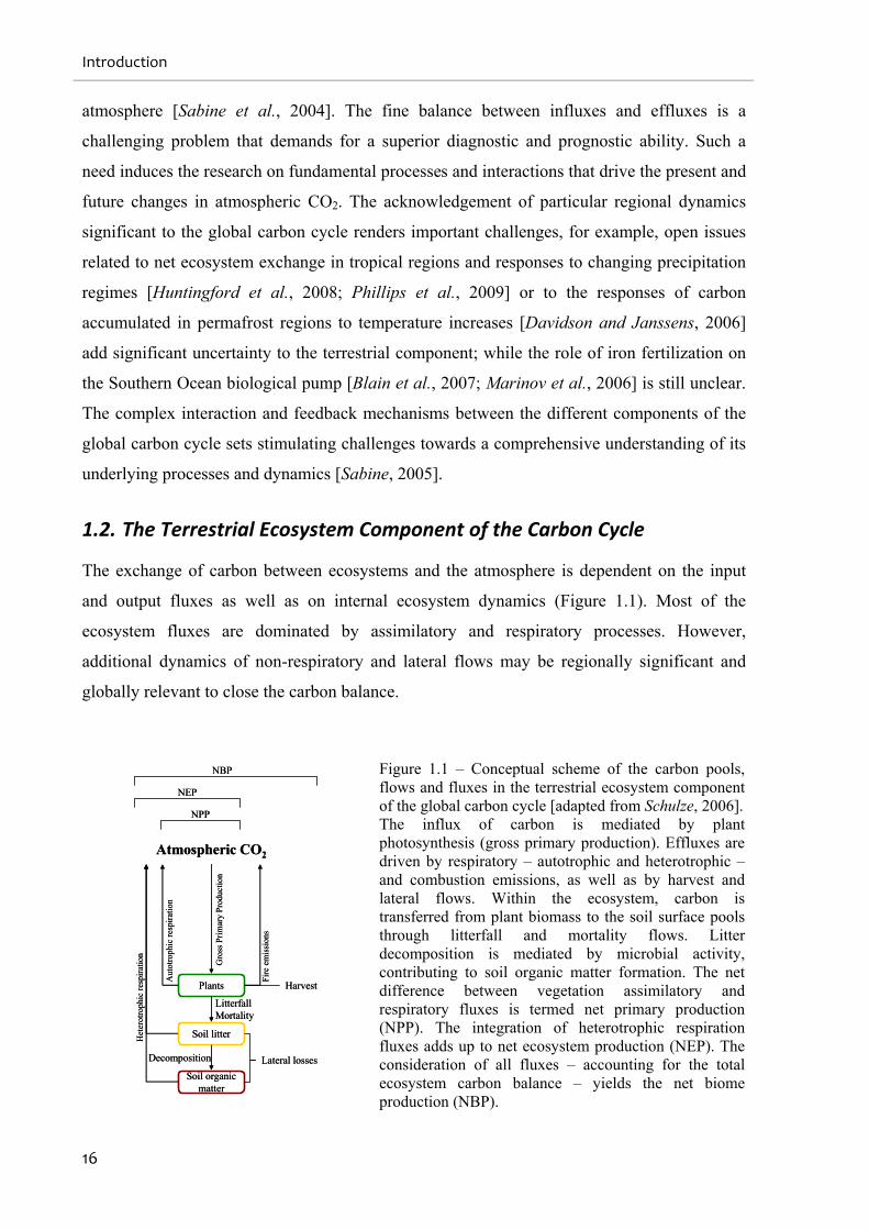
Figure 1.1 – Conceptual scheme of the carbon pools, flows and fluxes in the terrestrial
ecosystem component of the global carbon cycle [adapted from Schulze, 2006]. ................... 16
Figure 1.2 – Conceptual workflow of a model data integration approach [adapted from
Mahecha, 2009; Williams et al., 2009]..................................................................................... 45
Figure 1.3 – Location and characterization of the Iberian Peninsula in its two most significant
bioclimatic regions: Temperate and Mediterranean [source: EEA, 2008]................................ 51
Figure 2.1 – ANOVA test results on the four model performance indicators yielded by the
CASA model optimization throughout sites (FST) and temporal resolutions (TMR) for all
parameter sets considered (PRM)............................................................................................. 94
Figure 2.2 – MEF distribution for simulations where η is considered in the parameter set
(CCSSAr). ................................................................................................................................. 94
Figure 2.3 – CASA model NEP estimates for IT-Non at different temporal scales................. 96
Figure 2.4 – Observations versus simulations results between different parameter sets and 0
(IT-PT1).................................................................................................................................... 97
Figure 2.5 – Comparison between model performances of the different parameter sets
considered in the optimization exercise: left – MEF; right – absolute NAE............................ 98
Figure 2.6 – Relationship between mean annual NEP observations and η optimization results
throughout parameter sets for daily calculations. ..................................................................... 99
Figure 2.7 – Results of the ANOVA on the optimized parameters variance explained by single
factors and interactions. .......................................................................................................... 100
Figure 2.8 – CCSSAr impact on ε* estimates......................................................................... 101
Figure 2.9 – Effects of η in optimized parameter constraints................................................. 102
Figure 2.10 – Results of the ANOVA on the optimized parameters uncertainties variance
explained by single factors and interactions........................................................................... 104
Figure 2.11 – Mean annual net ecosystem production (NEP) versus mean annual gross
List of Figures
8
primary production (GPP, r2 = 0.96, α < 0.0001) and ecosystem respiration (RECO, r2 = 0.002,
α < 0.91), estimated from flux partitioning.............................................................................105
Figure 2.12 – Comparison between total soil C pools field measurements (black), estimated by
the CASA model under relaxed (grey) and fix (white) steady-state conditions, considering
different temporal resolutions mean (filled bars) and standard deviation (error bars)............106
Figure 3.1 – The CASA and CASAG scheme of vegetation and soil level carbon pools:
overall, carbon flows from top to bottom................................................................................122
Figure 3.2 – Schematic representation of the “mechanistic” experiment principle used in
dynamic recovery setups: dynV , dyn
Vk and mixSV ; illustrating the evolution of C pools in time
after the prescribed disturbances in vegetation pools..............................................................124
Figure 3.3 – ANOVA results for the different model performance indicators used...............129
Figure 3.4 – Distribution across sites of model efficiency (MEF) and absolute normalized
average error (|NAE|) ratios between parameter vectors on xx-axis and empS ........................130
Figure 3.5 – Distribution across sites of parameter ratios between parameter vectors on xx-axis
and empS . .................................................................................................................................131
Figure 3.6 – Distribution of parameter uncertainties ratios between parameter vectors on xx-
axis and empS . ..........................................................................................................................134
Figure 3.7 – Contour plots for single constraint cost functions (NEP) and for the multiple
constraints cost function (NEP, AGB): integrating net ecosystem production fluxes (NEP) and
above ground biomass pools (AGB). ......................................................................................136
Figure 3.8 – Comparison of NEP MEF between multiple constraint cost functions (CFM –
considering pools and fluxes) and single constraint cost function (CFS – considering fluxes).
.................................................................................................................................................137
Figure 3.9 – The integration of pools in the cost function allows the differentiation between
different model structures by comparison of model efficiency (MEF, left); and allows
identifying model structures that enable the correct simulation of vegetation C pools as well
(right).......................................................................................................................................138
Figure 3.10 – Comparisons of the model efficiency (MEF) between empS and ηwood parameter
vectors ( empSV , mix
SV , dynVk and dyn
V ) for optimizations considering solely fluxes in the cost
function (single constraint cost function: CFS; 7a) and integrating vegetation C pools as well
9
(multiple constraint cost function: CFM; 7b). ......................................................................... 139
Figure 3.11 – Comparison between CASAG model simulations and site observations at FR-
Hes for different experimental setups..................................................................................... 142
Figure 3.12 – Development of vegetation and soil C pools in FR-Pue for three experimental
setups. ..................................................................................................................................... 144
Figure 4.1 – Abacus of NEPT decomposition into NPP and RH trends: NPPT and RHT,
respectively............................................................................................................................. 164
Figure 4.2 – Spatial patterns of the representativeness of the eddy-covariance sites for pixels
of the Iberian Peninsula. ......................................................................................................... 167
Figure 4.3 – The classification of the Iberian Peninsula according to the optimized eddy-
covariance sites per PFT (left column) is based on the selection of the closest site to each
pixel. ....................................................................................................................................... 168
Figure 4.4 – Influence of distance to equilibrium (η) in the inter-annual variability (IAV) in
net ecosystem fluxes (a) and in the IAV in the de-trended NEP fluxes (removing the sole
recovery from the C pools) (b). .............................................................................................. 169
Figure 4.5 – Influence of distance to equilibrium (η) in the IAV in heterotrophic respiration
(RH) fluxes (a) and in the IAV in the de-trended RH fluxes ( DHR , removing the sole recovery
from the C pools) (b). ............................................................................................................. 170
Figure 4.6 – The distribution of the NEP trends (Sen slopes, gC.m-2.yr-2) is strongly dependent
on η values (a) while for NEPD its distribution appears invariant with η (b). ........................ 171
Figure 4.7 – Mean significant trends in NEPD, NPPD and DHR (gC.m-2.yr-2)......................... 172
Figure 4.8 – Decomposition of NEPD trends into DHR and NPPD trends ( D
TNEP , DTRH and
DTNPP , respectively – gC.m-2.yr-2) (a).................................................................................... 173
Figure 4.9 – Decomposition of NPPD trends (gC.m-2.yr-2) into Tε and fAPAR trends, TεT and
fAPART, respectively (fractional units per square meter per year) (a)................................... 174
Figure 4.10 – Decomposition of NPPD trends (gC.m-2.yr-2) into Wε and fAPAR trends, WεT
and fAPART, respectively (fractional units per square meter per year) (a)............................ 175
Figure 4.11 – Decomposition of DHR trends (gC.m-2.yr-2) into Ts and substrate availability
trends, TsT and SAT, respectively (a)...................................................................................... 175
List of Figures
10
Figure 4.12 – Decomposition of DHR trends (gC.m-2.yr-2) into Ws and substrate availability
(SA) trends, WsT and SAT, respectively (fractional units per square meter per year) (a).......176
Figure I.1 – MODIS fAPAR time series resulting from different treatment methods. ...........202
Figure II.1 – Effect of optimum temperature (Topt) on light use efficiency estimates. ...........206
Figure II.2 – Impact of the Q10 parameter on the effect of temperature on soil biological
activity (Ts)..............................................................................................................................208
Figure II.3 – Sensitivity of the below ground soil moisture effect (Ws) to the water storage to
monthly PET ratio (Bgr) for different Aws estimates (Ts)......................................................209
Figure V.1 – Changes between empV and
model efficiency (MEF; left) and normalized
average error (NAE; right) by integrating a parameter that only affects the slow turnover
vegetation pools after equilibrium (ηW in empV )......................................................................220
Figure V.2 – Comparison of model performance statistics between CASAG and CASA: a)
normalized average error (NAE); and 2) modelling efficiency (MEF). .................................221
Figure V.3 – Relationship between CASA and CASAG maximum light use efficiency
estimates – ε* and *g , respectively – (a), and CUE for CASAG (b). .....................................222
Figure V.4 – Global relationship between NPP and GPP for site level optimization.............223

11
List of Tables
Table 2.1 – Identification of the different sites included in the parameter optimization
analysis. .................................................................................................................................... 86
Table 2.2 – Parameters used in the different model optimizations. ......................................... 90
Table 2.3 – Identification of the different parameters included in each parameter set. ........... 91
Table 2.4 – Model performance results for different temporal resolutions (mean ± standard
deviation). ................................................................................................................................. 93
Table 2.5 – Frequency of correlation degrees at different temporal resolutions of correlation
matrix results from parameter optimization. ............................................................................ 95
Table 2.6 – Parameter optimizations results for 0 at daily temporal scale per site (parameters
standard errors in parentheses). .............................................................................................. 101
Table 2.7 – Results for the parameters’ standard errors (SE) mean and standard deviation
considering both a fix CCSSA (CCSSAf) and a relaxed CCSSA (CCSSAr). ........................ 104
Table 3.1 – Results for the parameters’ standard errors (SE) mean and standard deviation
considering both a fix CCSSA (CCSSAf) and a relaxed CCSSA (CCSSAr). ........................ 121
Table 3.2 – Identification of the different η-type scalars introduced in each parameter vector
(θ)............................................................................................................................................ 123
Table 3.3 –Model performance differences between CASA and CASAG across sites and
parameter vectors.................................................................................................................... 129
Table 3.4 – Mean normalized differences (%) of both optimized parameter estimates and
parameters uncertainties (values in parenthesis) between empS and the other parameter vectors
(having empS as the reference). ............................................................................................... 132
Table 3.5 – Differences between the Akaike information criterion (AIC) and the minimum
AIC (AICmin) for each experiment for each site. .................................................................... 133
Table 3.6 – Parameter optimization results for multiple constraints approaches. .................. 140

List of Tables
12
Table 4.1 – Identification of the different sites included in the parameter optimization. .......157
Table 4.2 – Acronyms used to identify the different ecosystem flux components and temporal
signals......................................................................................................................................163
Table 4.3 – Results of the site level parameter optimization organized by plant functional type
(PFT). ......................................................................................................................................165
Table 4.4 – N-way ANOVA results (%) for each optimized parameter for each factor.........166
Table 4.5 – Percentage of positive, negative and non significant trends in NEPeq and NEPD for
the Iberian Peninsula. ..............................................................................................................172
Table 4.6 – Results for the decomposition of NEP trends into NPP and RH trends for NEPD
and NEPeq. ...............................................................................................................................173
Table 4.7 – Partial correlations between the trends in NPPD ( DTNPP ) and D
HR ( DTRH ) and
trends in its drivers. .................................................................................................................174
Table III.1 – Correspondence between correlation ranges and text referred. .........................213
13
Chapter 1 – Introduction
The global carbon cycle is of significant interest in the context of climate dynamics. For long
the effects of increasing atmospheric carbon dioxide in the Earth’s climate have been a subject
of interest [Arrhenius, 1896]. The radiative forcing capacity of massive and continuous
emissions of carbon dioxide from fossil fuel combustion to the atmosphere since the early
Industrial Era was then linked to the climate system and significant increases in atmospheric
temperatures were foreseen. Today these effects are still corroborated by diverse approaches
involving global climate modelling and paleoclimatic methods [Field et al., 2004; Solomon et
al., 2007], although significant debate still surrounds these issues. Knowledge on the internal
mechanisms and feedbacks between the different components of the carbon cycle has evolved
significantly since then [Field and Raupach, 2004]. However, the diagnostic and prognostic
needs and uncertainties emphasize the current limitations and drive the active research on the
Earth system science, which ultimately lead to advances in process understanding.
The recognition of the tight association between living organisms and the Earth’s physical
components by geologist Vladimir Vernadsky in 1922 was instrumental to explain the
distribution of the different elements [Ollinger et al., 2003]. By introducing Biogeochemistry
as a discipline [Vernadsky, 1998], Vernadsky’s vision triggered research that revealed the
Biosphere as a relevant Earth system component [Ollinger et al., 2003]. Key posterior works
developed conceptual models for the cycling of elements through biological systems [e.g.
Redfield, 1958] and suggested continuous feedbacks between the atmosphere and terrestrial
ecosystems [Deevey, 1970; Rastetter et al., 1997]. The underlying – and many times implicit
– concepts of ecological stoichiometry set a common framework for the research of
interactions and feedback mechanisms [Melillo et al., 2003a]. The terrestrial biosphere is an
active component of the global biogeochemical cycles and its relevance is further emphasized
in the context of global climate dynamics by its role in the carbon and water cycles [Melillo et
al., 2003b; Schlesinger, 1997].
A strong research effort that aims to improve understanding in the terrestrial biosphere
component of biogeochemical cycles is in progress. Currently, active research involves
observational improvements, analysis and synthesis approaches, as well as modelling efforts
Introduction
14
that range from the sub-cellular level to regional and global scales. Optimally, process-level
observations should complement the prior knowledge on the focused systems and enhance the
predictability power. However, the complexity of biological and ecological open systems and
the difficulties in isolating factors often undermines understanding [Oreskes et al., 1994]. The
consequent deductive process is limited and involves significant simplification or implies
some assumptions at best. The increasing availability of observational datasets and numerical
analysis tools encourage the challenge of existing theories on terrestrial ecosystems in the
context of the carbon cycle.
1.1. The Global Carbon Cycle
Accounting for the carbon storage and fluxes between the major Earth components –
Cryosphere, Lithosphere, Hydrosphere, Biosphere and Atmosphere – is essential for
monitoring the global carbon cycle. Most of the Earth’s carbon is kept in the Lithosphere,
stored in sedimentary rocks, and only a small portion is in active pools – with turnover times
shorter than decades or centuries – near the Earth’s surface [Schlesinger, 1997]. The oceanic
carbon pool is by far superior to the land (vegetation, soils and detritus) and atmospheric
reservoirs [Denman et al., 2007]. Despite the differences between the magnitudes of these
reservoirs, their relative sink capacity for emissions from fossil fuel combustion and land use
change is comparable [Canadell et al., 2007b]. Accordingly, understanding the internal
dynamics and interaction of each reservoir is equally relevant within the context of the global
carbon cycle.
In the last four decades the atmosphere has been the carbon sink for ≈43% of the annual
emissions from fossil fuel and land use change – carrying the associated radiative forcing –
and the remainder 57% are distributed between oceans (≈27%) and land (≈30%) [Canadell et
al., 2007b; Le Quéré et al., 2009]. The absorption of carbon dioxide by the ocean and land
pools scales with its atmospheric concentration causing the current atmospheric levels to be
lower than if all CO2 emissions had remained in the atmosphere. However, increases in the
airborne fraction of CO2 emissions since 2000 may stem from slower responses or saturation
of land and ocean reservoirs to increasing CO2 emissions [Le Quéré et al., 2009], which yield
a “stronger-than-expected and sooner-than-expected climate forcing” [Canadell et al., 2007b],
although this is still under debate [Knorr, 2009]. The removal of CO2 from the atmosphere to
the other active pools is mediated by chemical and biogeochemical reactions that entail
particular interactions and feedbacks. Understanding the processes responsible for the
The Global Carbon Cycle
15
exchanges between and within active carbon pools is fundamental for estimating current – and
to anticipate future – impacts of human activities in the Earth’s climate system.
In the ocean, following Henry’s Law, the influence of wind speed [e.g. Wanninkhof and
McGillis, 1999] and water “skin” temperature [e.g. Archer, 1995] on CO2 solubility in water
controls most the atmosphere-ocean flux [Schlesinger, 1997]. Based on Henry’s Law we
would expect an increased CO2 dissolution in the ocean resulting from the rising atmospheric
CO2 concentrations [Tans et al., 1990]. The process is limited by the available contact surface
between the atmosphere and the ocean and the speed of vertical water exchange [Schlesinger,
1997]. Hence, the ocean absorption rate of CO2 from the atmosphere is limited by mixing of
surface and deep waters, which mainly occurs in Polar regions with the formation of bottom
waters [Schlesinger, 1997]. Further, biotic processes associated to photosynthesis at the
surface [e.g. Tans et al., 1990] and to the downward transport of living and dead organisms
[e.g. Taylor et al., 1992] are an active supply of organic carbon to deeper ocean bacterial
communities [Schlesinger, 1997]; which is then mostly oxidized by heterotrophic activity
[Sabine, 2005], returning to the atmosphere in upwelling zones. Current results on the effects
biological activity on contemporary ocean-atmosphere carbon fluxes emphasize the relevance
of biotic processes, in addition to physical processes [e.g. Le Quéré et al., 2005; Le Quéré et
al., 2007].
The carbon fluxes between the terrestrial biosphere and the atmosphere are mostly controlled
by photosynthetic and autotrophic and heterotrophic respiration processes. The atmospheric
CO2 observations from Mauna Loa reflect the influence of the Northern Hemisphere’s
biosphere activity on the seasonality of CO2 concentrations [Keeling et al., 1996]. But the
responses of vegetation to climatic patterns occurring at inter-annual time scales, like El Niño
– La Niña cycles, are also identified in the CO2 record [e.g. Keeling et al., 1996; Myneni et al.,
1997]. The exchanges of energy, water and carbon between terrestrial biosphere-atmosphere
interactions are tightly coupled, highly nonlinear and occur at multiple time scales, rendering
significant uncertainties in terms of mechanisms and feedbacks [Heimann and Reichstein,
2008]. Changes in climate and/or environmental conditions generate responses from the
terrestrial biosphere that can either dampen or amplify changes in these climate forcing,
yielding negative or positive feedbacks, respectively [Bonan, 2008]. The terrestrial biosphere
embodies processes and dynamics of significant relevance and special scientific interest in the
context of the global carbon cycle.
On a global scale, the strength of the terrestrial photosynthetic uptake is close to the
respiratory fluxes. Analogously, the ocean influxes are nearly balanced by effluxes to the
Introduction
16
atmosphere [Sabine et al., 2004]. The fine balance between influxes and effluxes is a
challenging problem that demands for a superior diagnostic and prognostic ability. Such a
need induces the research on fundamental processes and interactions that drive the present and
future changes in atmospheric CO2. The acknowledgement of particular regional dynamics
significant to the global carbon cycle renders important challenges, for example, open issues
related to net ecosystem exchange in tropical regions and responses to changing precipitation
regimes [Huntingford et al., 2008; Phillips et al., 2009] or to the responses of carbon
accumulated in permafrost regions to temperature increases [Davidson and Janssens, 2006]
add significant uncertainty to the terrestrial component; while the role of iron fertilization on
the Southern Ocean biological pump [Blain et al., 2007; Marinov et al., 2006] is still unclear.
The complex interaction and feedback mechanisms between the different components of the
global carbon cycle sets stimulating challenges towards a comprehensive understanding of its
underlying processes and dynamics [Sabine, 2005].
1.2. The Terrestrial Ecosystem Component of the Carbon Cycle
The exchange of carbon between ecosystems and the atmosphere is dependent on the input
and output fluxes as well as on internal ecosystem dynamics (Figure 1.1). Most of the
ecosystem fluxes are dominated by assimilatory and respiratory processes. However,
additional dynamics of non-respiratory and lateral flows may be regionally significant and
globally relevant to close the carbon balance.
Gro
ss P
rim
ary
Pro
duct
ion
NPP
Aut
otro
phic
res
pira
tion
Plants
Soil litter
Soil organic matter
Atmospheric CO2
Het
erot
roph
ic r
espi
rati
on
Fire
em
issi
ons
Harvest
Lateral losses
NEP
NBP
LitterfallMortality
Decomposition
Gro
ss P
rim
ary
Pro
duct
ion
NPP
Aut
otro
phic
res
pira
tion
Plants
Soil litter
Soil organic matter
Atmospheric CO2
Het
erot
roph
ic r
espi
rati
on
Fire
em
issi
ons
Harvest
Lateral losses
NEP
NBP
LitterfallMortality
Decomposition
Figure 1.1 – Conceptual scheme of the carbon pools, flows and fluxes in the terrestrial ecosystem component of the global carbon cycle [adapted from Schulze, 2006]. The influx of carbon is mediated by plant photosynthesis (gross primary production). Effluxes are driven by respiratory – autotrophic and heterotrophic – and combustion emissions, as well as by harvest and lateral flows. Within the ecosystem, carbon is transferred from plant biomass to the soil surface pools through litterfall and mortality flows. Litter decomposition is mediated by microbial activity, contributing to soil organic matter formation. The net difference between vegetation assimilatory and respiratory fluxes is termed net primary production (NPP). The integration of heterotrophic respiration fluxes adds up to net ecosystem production (NEP). The consideration of all fluxes – accounting for the total ecosystem carbon balance – yields the net biome production (NBP).
The Terrestrial Ecosystem Component of the Carbon Cycle
17
1.2.1. Fundamental concepts
Terrestrial ecosystems remove carbon dioxide from the atmosphere through photosynthesis,
where sunlight mediates the production of carbohydrates and molecular oxygen from CO2 and
water [Schlesinger, 1997]. These exchanges are observed at the leaf level, where the influx of
CO2 and the efflux of O2 and water occur through the stomata [Jones, 1992]. This carbon gain
is denominated gross primary production (GPP). The efflux of CO2 from plants results from
metabolic respiration which supports growth and maintenance processes. This flux is named
autotrophic respiration (RA) and it is often partitioned in growth (RG) and maintenance (RM)
respiratory fluxes, according to the associated process [Amthor, 2000]. The net balance of
carbon in vegetation is:
ARGPPNPP , (1.1)
where NPP is the net primary production (NPP). Through photosynthesis, vegetation is the
main source of organic carbon essential to the metabolism of ecosystems. The release of CO2
resulting from the microbial decomposition of organic carbon is defined as heterotrophic
respiration (RH). At the ecosystem level, the net balance of these fluxes is net ecosystem
production (NEP, Figure 1.1) [Schulze and Heimann, 1998; Schulze, 2006] and can be simply
defined as:
HHA RNPPRRGPPNEP . (1.2)
The processes and pools underlying these fluxes are strongly associated between them: RA is a
function of GPP and plant biomass [Amthor, 2000]; and the substrate availability for RH is
strongly determined by the magnitude and quality of vegetation pools and the transfer rates
from living vegetation to dead soil level pools [Trumbore and Czimczik, 2008]. Additionally,
at the landscape scale, non respiratory ecosystem losses of carbon are usually attributed to fire
(F), harvest of agricultural and wood products (H) [Körner, 2003] as well as lateral transport
(L), yielding net biome production (NBP, Figure 1.1) [Schulze and Heimann, 1998]:
LHFNEPNBP . (1.3)
Fire and harvest fluxes can be significant at ecosystem and regional scales, and are essential in
closing carbon budgets at global scales [Körner, 2003]. In general, the balance of the lateral
transport of carbon through erosion and runoff is assumed minimal at local scales but the
spatial variability may be high. NBP represents a full accounting of the terrestrial carbon
balance, which is beyond the scope of the current research objectives.
Introduction
18
1.2.2. Climatic drivers: responses and interactions
Terrestrial photosynthesis is strongly driven by the sunlight spectrum ranging from 400nm to
700nm, known as photosynthetically active radiation (PAR). But photosynthesis also:
responds nonlinearly to temperature changes [e.g. Berry and Bjorkman, 1980]; decreases with
increasing atmospheric water evaporative demand [e.g. Stockle and Kiniry, 1990]; and with
low water supply through reductions in stomatal conductance [e.g. Medlyn et al., 2001].
Changes in atmospheric concentrations of CO2 correlate positively with photosynthesis by
changing the difference between the atmospheric and leaf internal CO2 partial pressures
[Collatz et al., 1991; Norby et al., 2003]. Additionally, photosynthesis is mediated by
nitrogen-rich enzymes, which render the dependence of GPP to the nitrogen content of the
leaf tissue [McGuire et al., 1995].
The temperature controls on RA are associated to its influence on the rates of enzymatic
activity in cellular maintenance processes [e.g. Amthor, 2000], hence associated to RM. The
need for investment in maintenance processes increases with plant biomass and nitrogen
content [Ryan, 1991] and raises RM. Further, the leaf nitrogen content is expected to influence
RG indirectly by increasing GPP. Similarly, the influence of higher atmospheric CO2
concentrations on RG yields from increases photosynthesis and growth. Additionally,
increasing whole plant size would also raise maintenance and RM [Amthor, 2000]. The water
stress effects on RA are mainly explained by reductions in GPP (reducing RG) [Hanson and
Hitz, 1982] but slowly exposing plants to water stress can also yield reductions in
maintenance activities and consequently on RM [Ryan, 1991].
Like in RM, the response of microbial decomposition to temperature is based on the principles
of enzymatic kinetics, rendering the RH fluxes strongly dependent on temperature [Kätterer et
al., 1998; Kirschbaum and Farquhar, 1984; Lloyd and Taylor, 1994]. The response of RH to
soil water availability is highly nonlinear, significantly reducing RH under very dry (limiting
substrate diffusion in water films and/or desiccation) or very wet conditions (impeding O2
diffusion through the spoil pores) [Linn and Doran, 1984; Skopp et al., 1990]. Substrate
availability and quality are determining factors controlling decomposition rates, e.g.: labile
carbon originated from leaf fall or root exudates promote the faster decomposition rates
[Grayston et al., 1997; Lynch and Whipps, 1990]; oppositely to chemically recalcitrant carbon
pools. In this regard, adjustments in the structure of microbial communities responding to
changes in the quality of available substrate may change the decomposition patterns [e.g.
Curiel Yuste et al., 2007].
The Terrestrial Ecosystem Component of the Carbon Cycle
19
The different ecosystem fluxes are inherently coupled to surface climate variables and
between themselves. The unattainable observation of individual and interacting processes in a
full factorial way hampers the disclosure of “pure” mechanisms and interacting effects. It is
common to find varying response functions to analogous variables, including the responses of
photosynthesis to temperature [June et al., 2004; Medlyn et al., 2002]; the function of
stomatal conductance to vapour pressure deficit [Collatz et al., 1991; Leuning, 1995]; or the
response of RH to temperature [Kätterer et al., 1998; Kirschbaum and Farquhar, 1984; Lloyd
and Taylor, 1994]. Differences can originate from intrinsic differences between the observed
systems, from equally fit response functions for the observational datasets or from factors that
confound the “pure” driver-response functions (like covarying drivers, for example).
Ecosystem level approaches often assimilate different response mechanisms observed at
“individual” component scales. The difficult distinction between the varying functional
responses and sensitivities for a given process is often impeditive of generalization and
hampers prognostic abilities. For example, ecosystem influx (GPP) and efflux (RA and RH)
processes are positively correlated to temperature, which hinders the net effect of increasing
temperature on the ecosystem’s CO2 balance without an accurate estimate of individual flux
sensitivity. Studies at the ecosystem level focusing the response of net fluxes to interacting
mechanisms often emphasize the need of further process clarification. Additionally, Luo
[2007] highlights that the complexity of different mechanisms associated to warming trends is
beyond the kinetic sensitivities of fluxes, and include: phenological changes causing the
extension of the growing season [e.g. Myneni et al., 1997]; changes in species composition
favouring the adjustment to new water regimes [e.g. De Valpine and Harte, 2001] or nutrient
availability conditions [e.g. Chapin et al., 1995]; enhanced nitrogen mineralization [e.g.
Melillo et al., 2002]; and changes in ecosystem-water dynamics through changes in the
hydrological cycle [e.g. Huntington, 2006].
1.2.3. Effects of nitrogen on ecosystem processes
Another example of complex interaction mechanisms is the effect of nitrogen deposition on
the net ecosystem fluxes. Increasing deposition of nitrogen from the atmosphere may lead to
the accumulation of carbon in vegetation and soils [Nadelhoffer et al., 1999; Schlesinger and
Andrews, 2000] but the interactions with other elements and processes impede the detection of
a direct causal effect [Luo et al., 2004]. The effects of nitrogen deposition on NPP depend on
the form of nitrogen deposited and on the existent nitrogen loads. In low-nitrogen systems the
fertilization effect of nitrogen as NH3 on NPP appears to be positive. But in high-nitrogen
(saturated) systems, nitrified nitrogen leaches from the ecosystem carrying cations from soil
Introduction
20
surface and humic complexes [Austin et al., 2003]. The negative effects of such material
export from the system may exceed the effect of nitrogen fertilization on NPP, yielding NPP
decrements [Aber et al., 1998; Austin et al., 2003]. The spatial association of NOx and O3
yields a dual and contrary effect on NPP: fertilization by NOx that deposits in vegetation and
in soils as dry and wet deposition (NO + NO2) [Galloway and Cowling, 2002]; and reduction
of CO2 uptake caused by tissue damage upon exposition to tropospheric O3 [Aber et al., 1998;
Canadell et al., 2007a]. The effects of nitrogen on RH are dependent on the responses of NPP
and vary with the temporal scale of analysis. Increases in the litter quality can enhance fast
decomposition and build up a large fraction of recalcitrant soil organic matter [Berg et al.,
2001]. Oppositely, low nitrogen litter decomposes slower first but ends up loosing more
carbon [Berg et al., 1996]. Experimental evidence of positive, neutral and negative effects on
heterotrophic decomposition is presented by Austin et al. [2003]. Further, shifting soil
decomposition and mineralization rates may feedback on plant production by changing
nitrogen availability. Consequently, nitrogen driven changes in the global terrestrial
assimilatory and respiratory carbon fluxes are dependent on regional environmental
conditions as well as on changes in temperature and CO2 concentrations.
1.2.4. Increasing atmospheric CO2 concentrations
The changes in atmospheric concentration of CO2 were anticipated to impact positively
primary production – since CO2 is the substrate of photosynthesis – and consequently yield
positive effects on the ecosystems carbon storage capacity. Such effect was expected more
notorious in C3 plants for which the CO2 concentrations are still bellow the saturation levels
for photosynthesis [Jones, 1992]. But posterior differences in the CO2-induced growth
between C3 and C4 plants were not clearly different [Morgan et al., 2004a], since the increases
in atmospheric CO2 concentration reduce significantly stomatal conductance [e.g. Medlyn et
al., 2001; Morison, 1998]. The increases in CO2 assimilation of C4 plants are suggested to be
an indirect effect of reduced water losses through transpiration during water shortage periods
– consequently reducing the effects of drought stress on photosynthesis [Ainsworth and
Rogers, 2007]. However, the responses of photosynthetic activity and stomatal conductance to
increasing atmospheric CO2 change significantly between different plant functional groups
[Ainsworth and Rogers, 2007]. But frequently the observed stimulation of photosynthetic
activity by elevated CO2 concentration is not always paralleled by plant growth, since
increases in photosynthesis versus metabolic costs and different carbon allocation strategies
impede the direct assumption of growth upon photosynthetic stimulation [Körner et al., 2007].
The Terrestrial Ecosystem Component of the Carbon Cycle
21
The responses of microbial decomposition and heterotrophic respiration to increasing CO2
yield from the changes in vegetation dynamics that mainly translate changes in quantity and
quality of available substrate. But these responses can be divergent, for example: increases in
plant growth and in fine root production increase the substrate supply for decomposition
which can foment microbial respiration [in a forest, Heath et al., 2005] but can also reduce
nitrogen availability for microbial communities leading to reductions in decomposition [in a
grassland, Hu et al., 2001]. Further, the soil microbial communities can be affected by CO2-
induced changes in plant species composition and active tissue quality [Körner, 2000] and
quantity [Lesaulnier et al., 2008]; and increases in soil water availability that result from
reductions in stomatal conductance [e.g. Morgan et al., 2004a] that can either augment or
decrement soil respiration depending on the reference or seasonal soil moisture status.
Although the functional characteristics of plants are central, whole ecosystem responses are
highly dependent – and feedback on – environmental factors, such as nutrient (mainly
nitrogen) and water availability [e.g. Luo et al., 2004; Morgan et al., 2004b]. And in general,
there is a wide range in the net effects of rising atmospheric CO2 levels at the ecosystem scale.
The range of results currently considered stem from the diversity of intrinsic ecosystem
properties, environmental factors and climatic regimes as well as depends on the different
temporal scales of analysis [as proposed by the progressive nitrogen limitation ideas of Luo et
al., 2004], suggesting a significant geographical variability of the CO2-induced effects in the
biosphere-atmosphere interactions. Further, the ecosystem responses to CO2 treatments based
on instantaneous CO2 increments may significantly differ from the expected gradual
increments [Luo and Reynolds, 1999], deterring the direct generalization of observed
functional responses.
Carbon cycling within the ecosystem is directly affected by climate regimes, substrate and
nutrient availability depending on the plant and microbial communities’ responses to different
stimulus. Consequently, regional and local characteristics are instrumental for a global
analysis of the effects of projected changes in climate regimes, increasing atmospheric CO2
concentrations and nitrogen availability on the carbon cycle. A comprehensive integration of
these processes in global modelling exercises usually yields similar overall responses between
models, despite strong regional differences [Zaehle et al., 2010].
1.2.5. Land cover change and management regimes
Changes in vegetation communities can yield contrary effects on the carbon balance
depending on the prior and posterior ecosystem functional properties and response
Introduction
22
mechanisms. These can originate from gradual succession dynamics or changes in
environmental conditions that favour species adapted to new circumstances, from natural
ecosystem disturbances (see “Ecosystem disturbances” below) or from land cover conversions
induced by human activities.
Human-induced changes in vegetation are intrinsically linked to changes in the use of land;
usually imply transitions from natural to agricultural or agroforestry systems, changes in land
exploration regimes or crop/forest types. These often represent an abrupt perturbation with a
multiplicity of impacts including significant regional to global biodiversity losses and changes
in the ecosystem carbon cycles [Houghton et al., 1983]. The immediate emissions of carbon to
the atmosphere depend if the conversion from natural forests to agricultural or agroforestry
systems is mediated by fire or entails an interest in wood products. The initial phase of the
exploration period usually entails removals of vegetation carbon pools from harvest ending up
in reductions in fresh litter inputs to the soil. Consequently, microbial decomposition of more
recalcitrant pools occurs, leading to significant depletion of soil organic matter pools [e.g.
Mosier, 1998]. Currently, soil carbon losses due to native vegetation conversion to
agricultural systems are particularly problematic in tropical regions, where the majority of the
soil C losses occur within the first few years [Mosier, 1998; Paustian et al., 1997]. Further,
intensification of ecosystem carbon losses can be associated to reductions in soil fertility, soil
water holding capacity and erosion events, for example [Lal et al., 2004]. However,
appropriate management practices can minimize such effects by adequate fertilization, crop
rotation or increasing fallow periods and reduced tillage [Reganold et al., 1987]. Other
management practices can contribute significantly to carbon accumulation in these systems,
such as fire suppression, pest management and genetic manipulation.
Reforestation dynamics intrinsically entail higher storage of carbon at the ecosystem level, by
accumulating carbon in wood pools and supplying fresh litter for microbial decomposition.
The general observation of current sink conditions in European forests is assumed
significantly associated to reforestation activities during the last century [Nabuurs, 2004].
Also, the abandonment of land entails the re-growth of secondary vegetation, increasing
carbon accumulation in biomass and soil pools and creating a net carbon sink. Land
abandonment dynamics can contribute significantly to regional carbon budget estimates
[Vuichard et al., 2008].
Overall, the extent and intensity of human-induced land cover changes through deforestation,
reforestation, afforestation, cultivation, and logging activities contribute significantly to the
global carbon budget [e.g. Canadell et al., 2007b; Houghton, 2007]. Depending on
The Terrestrial Ecosystem Component of the Carbon Cycle
23
management regimes, local historical and current characteristics, land cover changes can
originate sink or source conditions. But land use changes are also consequential for other
biogeochemical cycles (like the water and nutrient cycles) and ecosystem biophysical
properties (such as albedo) [e.g. Denman et al., 2007]. Knowledge on the different dynamics
of land cover changes at regional scales is instrumental in global carbon budget calculations.
1.2.6. Ecosystem disturbances
Disturbances include low frequency high impact phenomena in ecosystem structure and/or
functioning. Perturbation regimes can constitute a dominant factor in several ecosystems
depending on their frequency and intensity. The main ecosystem disturbance processes
include fire, insect outbreaks, hurricanes, floods and other extreme weather.
Fire events restructure ecological succession stages by changing and driving changes in
vegetation communities [Odum, 1969]. Fire prone regions tend to favour vegetation
communities showing strategies adapted to the particular fire regimes [Pausas and Lloret,
2007]. At the landscape scale fire recovery is strongly dependent on site conditions like litter
fall quality and quantity, solar exposition, slope [Pausas et al., 2004b]; and fire regimes can
exercise controls on posterior vegetation communities by improving soil fertility [Pausas et
al., 2003] or by post-fire erosion [Mayor et al., 2007]. The CO2 emissions associated to fire
events are strongly dependent on fuel availability, and temperature and moisture conditions
[e.g. van der Werf et al., 2003]. And fire frequency and extension significantly contribute to
the role of fires in the carbon cycle context at global scales [e.g. van der Werf et al., 2004; van
der Werf et al., 2006]. Fires feedback positively to warmer temperatures by CO2 emissions to
the atmosphere; but can also yield negative feedbacks by posterior increases in biomass
accumulation and albedo [Goetz et al., 2007].
Other ecosystem perturbations driven by extreme weather events usually entail total or partial
destruction of vegetation structure [e.g. hurricanes, Chambers et al., 2007]. Biotic
disturbances refer to pests or insect outbreak which may attack different vegetation types and
components (e.g. trunks, bark, or leaves) with differing implications to the ecosystem carbon
cycle. These may extent from partial reduction in ecosystem carbon storage to the elimination
of important vegetation communities [e.g. Hogg et al., 2002]. Additionally, the effect of
climate projections on herbivore and pathogen communities may add up to the direct effect of
climate on the vegetation and ecosystem dynamics [Ayres and Lombardero, 2000].
The processes underlying the dynamics of the terrestrial component of the carbon cycle entail
different levels of organization; operate on different temporal and spatial scales; exhibit
Introduction
24
regional characteristics; and present internal and external feedback mechanisms. The
progressive increase in atmospheric CO2 levels and the increasing pressure of human-driven
activities on the natural systems urge for a comprehensive understanding of the dynamics,
mechanisms and feedbacks inherent to the terrestrial carbon cycle. Ultimately, it seems
sensible that the current research that has been emerging from different disciplines focuses
different aspects of the carbon cycle and adopts a wide variety of observational and modelling
tools to assist theoretical and experimental activities.
1.3. Methods for Observing Ecosystem Carbon States and Fluxes
Acquiring information about ecosystem properties or quantities is essential for its
characterization and, consequentially, lays the basis for learning. Relevant observations for
the terrestrial component of the carbon cycle include measurements of pools and fluxes as
well as of variables that influence or translate variations in ecosystem states.
1.3.1. Measuring ecosystem carbon pools
The net ecosystem-atmosphere fluxes are dependent on extrinsic drivers as well as on internal
ecosystem properties and substrate availability. The quantification of carbon pools has a
functional relevance in determining the sensitivity of ecosystem fluxes to its driving forces.
Misestimates of carbon pools may lead to erroneous estimates of flux responses to
environmental drivers, for instance: high leaf area index estimates may overestimate gross
primary productivity, or overestimations of labile carbon pools may yield stronger carbon
emissions upon increasing temperature scenarios. The proper quantification of available
carbon pools is essential to avoid misrepresentation of ecosystem fluxes sensitiveness to
environmental drivers. Furthermore, the quantification of different pools is informative on the
ecosystem’s internal carbon dynamics and its frequent monitoring may clarify carbon
pathways.
Harvest methods are the most reliable estimator of vegetation carbon pools and consist on
collecting vegetation samples and measuring the weight of the different vegetation
components (root, stem, branches, twigs, leafs) of tree, shrub and grass forms present in the
plot [Ravindranath and Ostwald, 2008]. In shrub or grass forms, biomass estimates rely
generally on harvesting and weighting sampled plots, but these methods are disadvantageous
for tree form inventories. To avoid harvesting methods, the in situ estimates of tree above
ground carbon pools often rely on measurements of surrogate parameters that assertively
relate to vegetation carbon stocks, such as diameter at breast height to estimate biomass [e.g.
Methods for Observing Ecosystem Carbon States and Fluxes
25
Brown and Schroeder, 1999]. Based on allometric equations, these measurements can be
subsequently converted to above ground biomass or total biomass. Often, estimates of below
ground biomass rely on analogous approaches concerning species or vegetation type specific
root to shoot ratios previously developed based on destructive measurements [e.g. Cairns et
al., 1997]. Site level estimates of leaf pools can be supported by leaf area index (LAI)
measurements with handheld instruments (e.g. LAI-2000) or hemispherical photography,
which can also provide in situ estimates of fAPAR and fraction of vegetation cover [Bacour et
al., 2006]. Recent remote sensing developments lead to the construction of a ground based
lidar instrument designed to capture forest structural parameters in a full upper hemispherical
footprint [the ECHIDNA instrument, Jupp et al., 2009]. Estimation of plant debris or litter fall
is essential for understanding the carbon balance at the tree level and to quantify the transfers
of carbon from live vegetation to the soil carbon pools. Usually, in situ observations rely on
litter traps that store falling matter or on litter collection campaigns spread in time to quantify
these carbon fluxes [Ravindranath and Ostwald, 2008].
Traditional methods to measure soil carbon pools require sampling soil in the field followed
by analytical estimates of organic carbon in the laboratory (ex situ measurements). Recent
developments for in situ measurements rely mostly on remote sensing and spectroscopy
concepts [Chatterjee et al., 2009]. These methods provide total soil organic carbon estimates.
But soils embody multiple timescales of carbon accumulation and decomposition that control
the storage of carbon. Hence, methods informative about the degradability or age – turnover –
of soil organic carbon are instrumental for the understanding of soil carbon dynamics
[Motavalli et al., 1994]. Incubation studies are informative on faster decomposition pools and 14C-dating techniques comprise time scales that range from 200 to 40000 years [von Lutzow et
al., 2007]. The distinction of soil compartments with different carbon turnover rates can be
determined by isotopic analysis of 13C tracing [Shang and Tiessen, 2000] or ‘bomb’ 14C
[Trumbore, 1993] and by chemical and physical fractionation methods [von Lutzow et al.,
2007]. Understanding the vulnerability of the different carbon pools to disruption mechanisms
and carbon stabilization mechanisms at multiple temporal scales is a critical issue in the
terrestrial biosphere component of the carbon cycle. Further, the development of these
methods is expected to support the conceptualization of soil carbon models that embody
multiple pools with different turnover rates. And, although some methods may reveal a
limited equivalence to conceptual pools [Smith et al., 2002; von Lutzow et al., 2007], a
reliable representation of modelled and measured pools seems possible under a careful
experimental design [Zimmermann et al., 2007].
Introduction
26
Overall, the development and unification of robust methods that are relevant at the process
scale is essential for understanding the role of individual carbon pools in the ecosystem
carbon cycle. In parallel, two important challenges are invariantly present in all of the above
measurement techniques: the spatial representation and upscaling of the measurements; and
the attribution of observational error to the measurements. An uncertainty estimate spans from
the measurement to the plot or ecosystem scale. For instance, the estimation of above ground
biomass based on diameter breast height should consider the uncertainties in: the diameter
breast height measurement; the empirical model used to estimate biomass; and in the scaling
method from tree to plot scale.
1.3.2. Observing net ecosystem carbon fluxes with eddy-covariance data
The eddy-covariance technique, first implemented by Swinbank [in 1951, Aubinet et al.,
2005], stems from broad scientific and technological developments in the field of
micrometeorology [Aubinet et al., 2001]. But it was in the early ‘90s that the first continuous
ecosystem level measurements began [Wofsy et al., 1993]. It is the first method that allows for
high frequency measurements of ecosystem-atmosphere fluxes of carbon, water and energy
[Baldocchi, 2003]. Eddy-covariance measurements encompass temporal and spatial scales
relevant to ecosystem processes: ranging from hours to years, and flux footprints that span
from hectares to several squared kilometres. These measurements have revolutionized
biogeochemical studies at ecosystem level since they are direct, non-destructive and
continuous observations of fluxes on the ecosystem scale.
The principles of eddy-covariance measurements are based on the conservation equation of a
scalar (c) and assume that its transport is mediated by vertical turbulent fluxes while lateral
gradients and molecular diffusion are negligible [Aubinet et al., 2000a; Baldocchi et al.,
1988]. After the application of the Reynolds decomposition – where a quantity, c, can be
expressed as the sum between the temporal average, c , and fluctuation around that average,
c , ccc [Aubinet et al., 2003] –, and assuming a null mean vertical velocity, the mean
flux density of c over some time (Fc) can be expressed as the covariance between fluctuations
in the vertical wind velocity (w) and the concentration c:
cwFc . (1.4)
By sampling CO2 in the turbulent vertical fluxes at high frequencies (10 to 20 Hz) in the
canopy-atmosphere interface, and assuming no storage or advection fluxes, Fc corresponds to
the net ecosystem exchange flux (NEP in Figure 1.1), which is usually aggregated to half
hourly or hourly periods [Baldocchi, 2003].
Methods for Observing Ecosystem Carbon States and Fluxes
27
From its underlying assumptions, the eddy-covariance measurements are mostly valid over
flat homogeneous terrain and under well developed turbulence and steady concentration
conditions [Aubinet et al., 2000a]. Under less favourable conditions (horizontal heterogeneity
and/or low turbulence conditions) the occurrence of advective air flows or storage violates the
method’s assumptions and may yield unreliable measurements. Atmospheric stratification
leading to storage is also more frequent in low turbulence nocturnal periods, impeding the
vertical mixing of air and consequently overestimating the sink capacity [e.g. Baldocchi,
2003]. But the storage of CO2 within the canopy can be disrupted at sunrise, when convective
turbulence occurs, and lead to an instantaneous overestimation of efflux from the ecosystem
[e.g. Baldocchi, 2003]. Canopy storage is a significant problem when resolving the daily cycle
of fluxes, but is not a critical issue from daily to annual time scales [Baldocchi, 2003] or if
measurements of vertical profiles are available [Aubinet et al., 2002]. In general, advection
fluxes may lend biases to net ecosystem flux estimations, varying in the vertical and
horizontal components [e.g. Aubinet et al., 2005]. The occurrence of advection during
nocturnal periods of low turbulence obstructs the measurement of night-time respiratory
fluxes, which may lend significant underestimation biases to respiration and general
overestimations of carbon sink conditions [e.g. Aubinet et al., 2005; Marcolla et al., 2005].
Further, since the advective air flows transport air to and away from the control volume, the
horizontal heterogeneity strongly determines the effects of advective fluxes on the EC
measurements [Aubinet et al., 2005; Feigenwinter et al., 2004; Marcolla et al., 2005]. Overall,
the violation of assumptions in eddy-covariance measurements can be insignificant
[Feigenwinter et al., 2004] or yield significant differences in estimating net ecosystem carbon
fluxes [Marcolla et al., 2005]. Ongoing research is actively focusing on methods to quantify
the different terms of the conservation equation but such procedures are far from operational
[e.g. Feigenwinter et al., 2008; Montagnani et al., 2009].
To circumvent these issues, applications of heuristic approaches rely on measurements of
friction velocity (u*) to identify periods of unfavourable turbulence conditions and reject
observational records [Aubinet et al., 2000b; Goulden et al., 1996; Papale et al., 2006].
Alternative approaches rely on the early night-time periods to parameterize monthly
temperature response functions used for the remaining hours of the night [Van Gorsel et al.,
2007]. The rejection of measurements, as well as system malfunctioning periods, leads
automatically to gaps in the observational time series. Gaps in the time series typically range
from 20% to 60% of half hourly records, which is sufficient for representing the daily cycle
but not for seasonal or yearly time scales (depending on the distribution of gaps) [Moffat et
Introduction
28
al., 2007], corroborating the development of gap-filling techniques. The modest contribution
of most gap-filling methods to biases in the annual sums of net ecosystem exchange (<
25gC.m-2.yr-1) lend confidence to robust gap-filling methods [Moffat et al., 2007].
Aiming at a proper representation of the ecosystem fluxes from daily to annual fluxes, gap-
filling techniques expand the usefulness of data time series for ecosystem model-data
integration approaches. But additional information of the measurement error characteristics is
important in such exercises, e.g. the selection of a cost function depends on the observational
error [Hollinger and Richardson, 2005; Lasslop et al., 2008]. The biases caused by night-time
low turbulence fluxes have been designated as a selective systematic error by Moncrieff et al.
[1996], in addition to the potential random and systematic observation biases. The random
error stems from instrument operation, from the stochastic properties of turbulence or from
varying footprints; and systematic errors yield from instrument calibration or systematic
missing high or low frequency components of the cospectrum. In a recent extensive
observational error characterization, Lasslop et al. [2008] analyzed half hourly eddy-
covariance measurements of carbon and water fluxes. Random error was shown to have small
auto and cross correlation and its magnitude scales with the magnitude of the fluxes
(heteroscedasticity), showing a La Placian distribution [also shown before by Hollinger and
Richardson, 2005; Richardson et al., 2006b], although the distribution of the random error
after normalization (by dividing each observation by its expected standard deviation) becomes
more Gaussian [Lasslop et al., 2008]. The discussion on the main properties of the random
error and its consequent role in defining optimization approaches in model data integration
exercises is still open [Williams et al., 2009]. In this regard, the consideration of robust
methods against outliers or violations of the assumed distribution represents a sensible
approach [e.g. least trimmed squares regression; Stromberg, 1997]. However, the temporal
averaging of ecosystem fluxes to daily or any coarser temporal scale reduces the random error
to absolute magnitudes below 5% [Baldocchi, 2003] and approximates its distribution to
Gaussian [Richardson et al., 2008]. Additionally, a proper instrument functioning and
calibration should significantly avoid systematic – but not selective – errors.
The eddy-covariance measurements integrate both carbon assimilation and release processes
(1.2), namely through photosynthetic (GPP) and respiratory processes (RH and RA, which sum
up to ecosystem respiration, RECO). From an ecological perspective, NEP measurements may
not suffice for interpreting ecosystem dynamics or for model evaluation since, for example,
increases in NEP can be caused by increases in GPP or decreases in RECO or both. Flux
partitioning algorithms aim at empirically separating both assimilatory and respiratory fluxes
Methods for Observing Ecosystem Carbon States and Fluxes
29
from the NEP signal based on ancillary data (e.g. temperature). One set of methods relies on
the diurnal cycle dynamics making use of nocturnal observations of ecosystem fluxes –
representing respiratory processes – to establish empirical relationships between flux and
meteorological variables. Daytime estimates of GPP are then estimated as the residuals
between estimated daytime RECO and NEP, or make use of non linear regressions between
GPP and environmental variables [Desai et al., 2008]. For instance, Reichstein et al. [2005]
partitioned the NEP fluxes using night-time observations to derive short term responses of
RECO to temperature, estimating GPP as the residual between NEP and daytime RECO; while
others relied on the day time parameterization of hyperbolic light response curves to partition
the diurnal fluxes into GPP and RECO [Lasslop et al., 2010]. Other methods based on the
construction of look up tables, the inversion of ecophysiological models or training neural
networks have also been developed [Desai et al., 2008; Moffat et al., 2007]. Site level
partitioning results can vary significantly amongst methods, especially for Mediterranean
systems. However, the ranking of GPP and RECO between sites is consistent between different
methods, implying a coherent spatial distribution of partitioned fluxes between methods
[Desai et al., 2008]. A proper evaluation of partitioning methods would necessarily involve
individual measurements of other flux components, such as evolution of soil or vegetation
carbon stocks, soil respiration or sap flow measurements, among others. Nevertheless, none of
these observational approaches are as operationally or representatively performed as eddy-
covariance measurements. Until verification arrives, the use of flux partitioned fluxes should
be cautious, moreover when different approaches can lead to different conclusions on the
performance of night-time or daytime-based methods [Desai et al., 2008; Stoy et al., 2006].
Ultimately, the global distribution of eddy-covariance towers aims at a wider
representativeness of the world’s ecosystems. Although still limited and biased in its
distribution, the measurements network has significantly grown in these last ten years
[Baldocchi, 2008]. It represents a unique information source and many valuable efforts have
been done to standardize procedures and organize a global database [Papale et al., 2006]. The
identification of issues and thriving improvements contribute to the confidence in the
representation of carbon, water and energy fluxes at the ecosystem level.
1.3.3. Remote sensing: an extensive information tool
Remote sensing has for long been recognized as a powerful tool for monitoring ecosystem
states given that healthy green vegetation possesses a particular spectral signature, as it
strongly absorbs in the visible and reflects in the near infrared regions of the spectrum. Light
absorption by photosynthetic pigments occurs most effectively in the visible region of the
Introduction
30
spectrum (especially in the blue and red regions), corresponding to an optimum trade-off
between the energy available for electron transport, weak enough to minimize damages in
biological structures [Bonan, 2002; Jones, 1992].
The consequent development of proxy variables – or vegetation indexes (VIs) – was based on
the combination of spectral information from red and near infrared reflectance channels, like
the normalized difference vegetation index (NDVI):
redNIR
redNIRNDVI
,
(1.5)
where NIR and red are, respectively, the near infrared and red reflectance retrievals from the
measurement instrument [Rouse et al., 1973; Tucker, 1979]. NDVI shows a significant
explanatory power of spatial and temporal variations of vegetation status throughout a wide
range of vegetation dynamics: spatial distribution of the seasonality of phenology [Alcaraz-
Segura et al., 2006]; determination of changes in vegetation cover and recovery patterns after
fire and logging events [Neigh et al., 2008]; decadal trends in photosynthetic activity [Myneni
et al., 1997; Slayback et al., 2003]; drought detection [Song et al., 2004]; among others.
But the passive satellite remote sensing signal of the earth surface within optical ranges is
prone to atmospheric contamination. Here, Kaufman and Tanré [1992] introduced an
atmospheric resistant vegetation index (ARVI) making use of the blue band to correct for
atmospheric contaminations effects. Further development of analogous vegetation indexes
aimed at minimizing the effects of soil background in areas of scattered vegetation [Huete,
1988] as well as saturation and atmospheric effects [Huete et al., 2002], among others. In this
regard, the enhanced vegetation index shows a significant reduction in signal saturation over
denser canopy covers and improvements in signal to noise ratios [Huete et al., 2002],
representing a robust alternative to NDVI for shorter term or finer spatial resolution studies.
Additional vegetation indexes explore different spectral regions for more specific
applications: Gamon et al. [1992] associated the photochemical reflectance index (PRI) to
photosynthetic light use efficiency, extending the applications of vegetation indexes to the
detection of changes in physiological states decoupled from greenness [e.g. Goerner et al.,
2009; Rahman et al., 2004]; Peñuelas et al. [1993] developed the water balance index (WBI),
which is correlated with the water content of the canopy; also for analogous purposes, Gao
[1996] developed the normalized difference water index (NDWI), and Ceccato et al. [2001]
evaluate the usefulness of the equivalent water thickness (ETW); the vegetation condition
index (VCI) [Kogan, 1995], for detection of drought impacts on vegetation status; and Hansen
Methods for Observing Ecosystem Carbon States and Fluxes
31
and Schjoerring [2003] explored normalized difference indexes as proxies for leaf nitrogen
concentration; among other examples. Although vegetation indexes show technical (e.g. need
for hyperspectral or narrower bands measurements, rarely available from satellite sensors)
and/or structural (e.g. different vegetation structures and states can yield similar vegetation
indexes) limitations, they comprise significant surrogates for the absorption of light by
vegetation, consequently being informative on photosynthetic processes. These can be
condensed in empirical associations between vegetation indexes and primary production [e.g.
Paruelo et al., 1997] or structural associations between vegetation indexes and biophysical
variables of terrestrial biosphere models, such as fAPAR and LAI [e.g. Myneni and Williams,
1994; Potter et al., 1993; Sellers et al., 1996].
The leaf area index (LAI) and fraction of absorbed photosynthetically active radiation
(fAPAR) are two vegetation biophysical properties intrinsically linked to vegetation states and
assimilatory fluxes, respectively, of the terrestrial carbon cycle. LAI and fAPAR are
intrinsically associated to each other and to NDVI [e.g. Asrar et al., 1992]. Although
empirical relationships between NDVI and fAPAR and LAI can be established [e.g. Sellers et
al., 1996], significant improvements in satellite remote sensing of fAPAR and LAI stem from
physically-based approaches derived from radiative transfer principles [Baret et al., 2007;
Gobron et al., 2000; Myneni et al., 2002]. These aim at the best approximation to the radiative
transfer problem solving for fAPAR and/or LAI with more or less assumptions about
vegetation structure. For instance, Myneni et al. [2002] make use of a land cover classification
to constrain vegetation structure parameters to yield fAPAR and LAI; while Gobron et al.
[2000] approximate fAPAR exploring all the scenarios used in the algorithm calibration
process; as well as Baret et al. [2007] for the CYCLOPES LAI, fAPAR and fraction of
vegetation cover products. The emergence of satellite remote sensing datasets of fAPAR and
LAI from multiple sensors based on radiative transfer principles sets ground for improving
diagnostics of the terrestrial carbon cycle. Similarly to vegetation indexes, the sensitivity of
fAPAR and LAI to changes in vegetation states renders them useful applications in analysis of
spatial patterns of drought spells [Ciais et al., 2005; Reichstein et al., 2007]; in biomass
mapping [Saatchi et al., 2007]; evaluation of leaf dynamics in post fire recovery periods [Liu
et al., 2005]; infer vegetation structure on moisture gradients [Scholes et al., 2004] and spatial
biogeographic patterns [Buermann et al., 2008]; among others. Further, the integration of
remotely sensed fAPAR provides inputs from site level primary production modelling [e.g.
Xiao et al., 2005], to regional [e.g. Jung et al., 2008] and global estimates [Zhao et al., 2005].
However, systematic disagreement between satellite retrievals of analogous quantities –
Introduction
32
mostly fAPAR – is a significant source of uncertainty. The assimilation of an uncertainty
equivalent to a systematic bias between different datasets leads to a directly proportional
increase in the uncertainty of primary production estimates, if the models are not re-
parameterized. The nature of divergent estimates can be associated to algorithmic and sensor
characteristics. But understanding the spatial and/or temporal variability of differences
between datasets could be more informative on the impacts in posterior modelling exercises.
Atmospheric conditions more or less affect all of the above measurements. The presence of
clouds, ozone, and other aerosols increase the absorption in the near infrared region usually
yielding underestimation spikes in vegetation indexes or vegetation biophysical properties
[e.g. Goward et al., 1991; Holben, 1986]. Commonly these are addressed through heuristic
correction methods such as the best index slope extraction [Viovy et al., 1992]; Fourier
transformations [Sellers et al., 1996]; temporal composites [Holben, 1986; Pinty et al., 2002];
asymmetric Gaussian functions fitting [Jonsson and Eklundh, 2002]; Savitzky-Golay filter
[Chen et al., 2004]; among others. Regardless of the methods’ complexity level, the main goal
of any strategy is the noise reduction in the time series of vegetation indexes or biophysical
properties. A recent comparison emphasizes the performance of sophisticated filtering and
function-fitting methods, although results are highly dependent on the phenology metric of
interest [Hird and McDermid, 2009]. However, future evaluations of different correction
strategies should include ecosystems subject to different dynamics, since filtering methods
may dampen the signal from disturbed or managed systems.
Further applications of remote sensing focusing vegetation states aim at estimating above
ground carbon pools. Often these approaches have been based on optical remote sensing and
compared to measurements of wood biomass from forest inventories, although showing
saturation effects for high density canopies [above 50 to 80 Mg/ha, Dong et al., 2003]. The
development of active radar based methods presents two significant advantages over optical
remote sensing: by measuring the microwave region of the spectrum, radar sensors are highly
insensitive to illumination and atmospheric conditions; and increasing wavelengths increase
the degree of penetration of measurements into the canopy until the soil surface, retrieving
information of the above ground biomass [e.g. Foody and Curran, 1994; Mitchard et al.,
2009]. The establishment of confidence bounds is a general limitation common in remote
sensing approaches and should include uncertainties in inventory data and mismatch between
in situ measurements and remote sensing footprint [Dong et al., 2003].
Overall, remote sensing contributes with measurements of ecosystem states that support
research on ecological disturbance and response processes and supply information for
Methods for Observing Ecosystem Carbon States and Fluxes
33
diagnostic modelling approaches. Further, satellite sensors provide systematic and spatially
explicit fields of observations relevant at ecosystem scales. Current challenges in satellite
remote sensing include effects of atmospheric conditions and instrument calibration on
reflectance retrievals, scale mismatches between in situ measurements and satellite footprint
and algorithmic robustness. Addressing uncertainty or minimizing representation mismatches
is essential since these observations support the construction of mental and/or mathematical
models on ecosystem functioning. Ultimately, methodological developments are potentially
extensive to regional and/or global applications. Additionally, hyperspectral remote sensing
has emphasized the large information content of the spectrum that can significantly amplify
the characterization ability of ecosystem states, although regional systematic measurements
are still unavailable [DeFries, 2008]. The SpecNet initiative may be instrumental at
addressing some of these issues through a network of in situ spectral measurements at
FLUXNET locations [Gamon et al., 2006].
1.4. Strategies for Terrestrial Ecosystem Modelling
In general, according to Liu and Gupta [2007], an ecosystem model can be considered as the
representation of an observable system with defined boundaries, across which fluxes of mass
and/or energy enter (inputs) and exit (outputs) the system. The quantities of mass and/or
energy stored in the system (model states or state variables) vary in time (and in space)
according to the responses of states-to-inputs and outputs-to-states embedded in the model
(model structure). Model behaviour is governed by characteristic properties of the system
(parameters) – assumed invariant in time – and can be significantly influenced to states prior
to the simulation (initial states). More or less explicitly, models embody assumptions and
conceptual principles about these aspects of the simulated systems depending on the
knowledge of the system or aim of the simulations, but also historical and practical reasons.
1.4.1. Modelling vegetation in ecosystem models
Multiple conceptual strategies stemming from different scientific areas have been adopted to
simulate the terrestrial biosphere including models of biogeography, dynamic (global)
vegetation and terrestrial biogeochemistry. The first models to emerge on global terrestrial
ecosystems were biogeography models that aim at predicting the spatial distribution of the
worlds biomes based on climate [Prentice et al., 2007]. Following the works of Alexander van
Humboldt’s in the early 1800’s and the temperature-driven classification of plants by
Alphonse de Candolle, Vladimir Koeppen (in 1884) was the first to formalize a climate-
vegetation classification scheme [Bonan, 2002]. Later, Holdridge [1947] developed a diagram
Introduction
34
associating macroclimate patterns to global distribution of different types of vegetation
[Bonan, 2002]. The conceptual association between climate and vegetation as been
extensively used in biogeography models that range from numerical classifiers that map
global plant functional types [Box, 1981], to statistical approaches [e.g. Hilbert and Ostendorf,
2001; Huntley et al., 1995] and more process-based approaches [e.g. Morin et al., 2008]. The
embodied concepts lend these models application from regional to global scales at coarser and
longer temporal scales [save due exceptions integrating finer spatial resolution variables, like
topography in Brzeziecki et al., 1993].
The spatial distribution of vegetation patterns is dominated by different mechanisms occurring
at different temporal scales that are not explained solely by climate-vegetation relationships
[e.g. Neilson, 1995]. Dynamic vegetation (or landscape) models, implicitly or explicitly,
embody the principles of population dynamics – growth, mortality, reproduction, dispersal
and competition for resources – and succession, in order to estimate spatial and temporal
changes in vegetation communities and eventually also biomass, production and nutrient
cycling [Bonan, 2002]. The objective and ability of dynamic vegetation models to simulate
transitions between biomes is unique amongst the different types of vegetation models.
Specially resolving changes in vegetation communities driven by changes in disturbance
regimes or disturbance events that significantly modify ecosystem structure and function. The
underlying concepts in dynamic vegetation modelling build on the works of Botkin et al.
[1972] and Shugart and West [1977] that simulate forest dynamics based on the
establishment, growth and mortality of individual trees [Bugmann, 2001; Perry and Enright,
2006; Prentice et al., 2007]. These concepts are also applied for non-forest systems, like
grasslands [Goslee et al., 2001] or shrublands [Nakayama, 2008]. But the potentially high
complexity and level of detail of these models impede global scale simulations. In this regard,
replacing deterministic by stochastic approaches for simulations of different process
simulations – like seed dispersal or fire propagation – allows a wider applicability of dynamic
vegetation models [Perry and Enright, 2006].
Transfer and storage of carbon through ecosystems in the context of the global carbon cycles
render different perspectives on vegetation and ecosystem processes. Terrestrial
biogeochemical models (TBMs) yield initially from the need to quantify net primary
production [Prentice et al., 2007]. TBMs develop on the assumption that primary production
is mainly controlled by environmental conditions (e.g. climate and nutrient availability) and
intrinsic vegetation properties. These models rely on more empirical or mechanistic
calculations of NPP and heterotrophic decomposition to estimate net ecosystem production.
Strategies for Terrestrial Ecosystem Modelling
35
Depending on the conceptual assumptions for primary production calculations, terrestrial
biogeochemical models can be further partitioned into production efficiency models or canopy
photosynthesis models [Ruimy et al., 1999]. Production efficiency models (PEMs) usually
follow the Monteith [1972] approach where primary production results from the efficiency (ε)
with which plants convert the absorbed photosynthetically active radiation (APAR) into
biomass. Since ε is regulated by temperature, water availability or other environmental
conditions, one common approach for estimating ε relies on the prescription of a maximum
light use efficiency rate (ε*) downgraded according to environmental stressors [e.g.
Mahadevan et al., 2008; Potter et al., 1993; Prince, 1991]. The general simplicity and
scalability are significant advantages for PEMs in biogeochemical modelling approaches.
Additionally, the availability of climate and vegetation biophysical spatially explicit fields
renders a wide application of PEMs at different temporal and spatial scales. Recent efforts
have explored the potential of a direct estimation of ε through PRI measurements from remote
sensors [e.g. Garbulsky et al., 2008; Goerner et al., 2009; Hilker et al., 2008]. Although still
insipient, these approaches embody significant amenability for regional and global
applications. On the other hand, canopy photosynthesis models usually embody more process-
based approaches for gross primary production [e.g. Collatz et al., 1992; Farquhar et al.,
1980] and autotrophic respiration, and explicit phenology simulations, allowing for prognostic
exercises given model climate drivers [e.g. McGuire et al., 1997; Running and Hunt, 1993].
Commonly, terrestrial biogeochemical models ignore processes of vegetation dynamics or
rely on model inputs to prescribe changes in vegetation or ecosystem types. These regulate the
functional responses of ecosystem to environmental drivers. Despite the consequent
limitations in prognostic ability, the general straightforward implementation of hypothetical
response mechanisms to different driving forces of ecosystem processes is a significant
advantage of TBMs.
Contemporary dynamic global vegetation models (DGVMs) aim to embody the most relevant
characteristics of these families of models to represent the biosphere system – atmosphere’s
lower boundary – in global climate modelling [Prentice et al., 2007]; often relying on detailed
description of vegetation biophysical and biogeochemical processes. The biggest difference
between more sophisticated TBMs and DGVMs is the latter ability to model vegetation
dynamics [Prentice et al., 2007]. Conceptually, DGVMs consider ecosystems as interactive
plant communities and should embed principles of plant development strategies, interaction
and succession processes, simultaneously to descriptions of carbon, water and nutrient cycling
within the ecosystem and exchange fluxes with the atmosphere. DGVMs present the highest
Introduction
36
complexity of terrestrial biosphere models [e.g. ORCHIDEE, Krinner et al., 2005; and LPJ,
Sitch et al., 2003], although entailing simplifications from the other approaches, for instance:
reducing an explicit population distribution to average individuals or the discrete mortality
approaches of dynamic vegetation models to average turnover times of vegetation carbon
pools; or considering heterotrophic decomposition approaches entailing less soil carbon pools,
although this is not always the case. The ultimate application goal of DGVM development is
its coupling with global climate models for simulations of future emissions scenarios
[Friedlingstein et al., 2006]. Global applications of DGVMs have been compared to past long
term trajectories of atmospheric CO2 concentrations [Prentice et al., 2007]; as well as
provided contemporary simulations of NBP fluxes at regional scales supported by
independent observational datasets [Piao et al., 2009]. Evaluation of DGVMs performance at
ecosystem scales is also instrumental in inferring uncertainty of global estimates and several
exercises have highlighted its advantages and limitations [e.g. Cramer et al., 1999; Mahecha
et al., 2009; Morales et al., 2007].
Overall, the distinction between the different modelling strategies may be shrinking as the
development of new DGVMs gradually incorporates more ecological processes supported by
increasing computational power and scientific understanding. The integration of additional
processes to increase the representation power of models presents clear trade-offs between
complexity and tractability by demanding more input variables and parameters. Contrasting
complexities are independent from spatial or temporal domains, transversely observed from
plot level (e.g. differences between detailed ecophysiology [Dufrêne et al., 2005] and stand
growth [Landsberg and Waring, 1997] models) to regional and global terrestrial biosphere
models (e.g. differences between TBMs and DGVMs). Model intercomparison exercises
highlight limits and/or uncover output differences between modelling approaches [Cramer et
al., 1999; Jung et al., 2007; Mahecha et al., 2009; Morales et al., 2005]. These exercises
embody the concept that the meaningfulness of model complexity – or simplicity – depends
on the modelling goals.
1.4.2. The treatment of soil level processes
One commonly observed feature throughout the different modelling approaches is the inferior
modelling complexity in simulating soil processes comparatively to vegetation processes
[Heimann and Reichstein, 2008; Pitman, 2003]. The treatment of soil decomposition and
mineralization processes ranges through a wide complexity of models.
Strategies for Terrestrial Ecosystem Modelling
37
Simple models consist of empirical approaches on decomposition processes estimating whole
soil respiration fluxes based on regression analysis [Luo and Zhou, 2006; Richardson et al.,
2006a]. The early association between enzymatic activity and temperature supports commonly
considered positive responses of soil respiration to temperature [e.g. Arrhenius, 1898; Frank
et al., 2002; Jenkinson, 1990; Lloyd and Taylor, 1994; van't Hoff, 1898]. Functional links
between soil moisture and respiration are harder to establish due to confounding effects
between actual effects of water availability in microbial decomposition and transport
mechanisms that, for example, limit O2 diffusion in the soil or alter substrate availability [Luo
and Zhou, 2006]. However, different approaches have demonstrated the advantages in
integrating empirical responses of soil respiration to water availability conditions [e.g.
Davidson et al., 2000; Reichstein et al., 2003a]. Additional approaches express the effects of
substrate availability on soil respiration by integrating information on vegetation states [e.g.
LAI, Curiel Yuste et al., 2007; Reichstein et al., 2003a] or productivity [e.g. GPP, Janssens et
al., 2001] as modelling proxies. The inclusion of multiplicative factors translating a functional
link between soil respiration and different environmental driving factors are a common
approach towards empirical modelling improvement [e.g. Reichstein et al., 2003a].
Process-based modelling approaches embed explicit representations of carbon cycling in the
soil media. More complex models simulate decomposition as well as mineralization
processes, providing nitrogen is explicitly represented in addition to carbon cycling. Carbon
and nitrogen inputs to the soil originate from vegetation processes such as litter fall, root
decay and exudates, which can be more or less explicitly simulated. Soil carbon is organized
in pools that represent reservoirs with different decomposability and mineralization rates.
Transfers of carbon between different pools are mediated by microbial activity [Parton et al.,
1987]. On a recent analysis, Manzoni and Porporato [2009] performed an extensive
comparison between the structural and conceptual basis of numerous (~250) biogeochemical
models. Various classes of models, characterized according to application purposes, differ in
complexity depending on alternative description approaches on decomposition and
mineralization processes. Most models assume donor controlled decomposition rates, even
when holding microbial pools, implicitly assuming microbial activity is never a limiting factor
[Manzoni and Porporato, 2009]. Mineralization schemes differ in the general pathway of
organic nitrogen between microbial and mineral pools, shifting between approaches that
consider mineralization occurs prior to microbial assimilation and approaches that consider a
direct assimilation of organic N by microbes – following mineralization –, or different
combinations of both. Although C to N ratios exert important controls on microbial activity,
Introduction
38
hence on decomposition, most model structures overlook changes in C to N availability, save
due exceptions. Interestingly, although soil microbiology models clearly show the highest
theoretical consistence in terms of modelling decomposition structures, the difference between
mineralization and nitrogen limitation schemes is not so significant. And generally slight
differences in modelling approaches are observed between the plot, ecosystem and global
scale models.
However, regional and global models, such as TBMs and DGVMs, commonly rely on
simplified versions of other models (e.g.: RothC or the CENTURY models) that embody
fewer pools, rely on implicit or neglect nitrogen cycling, or ignore temporal variations of
nitrogen limitation on microbial communities. Simplification stems from practical options
considering modelling tractability and computational demands. Simple schemes may also be
corroborated by the insufficiency of available information to disentangle the controlling
factors of soil respiration [Reichstein and Beer, 2008], even in simple empirical models.
1.4.3. Plant functional types
The classification of vegetation communities according to function represents a clear
simplification of plant life complexity. Existing plant diversity holds a multiplicity of
structural and functional characteristics that is well beyond the extent of a classification
scheme. Classifying vegetation according to function – plant functional types, PFT –
ultimately aims at individualizing groups with similar behaviour regarding responses to
environmental conditions, effects on ecosystem structure and inherent processes [Lavorel et
al., 2007]. Selecting measurable plant structural characteristics and traits amenable with
functional characteristics is instrumental for synthesis exercises and mapping purposes. PFT
classes convey information about vegetation behaviour which is of significant interest in
modelling exercises [Neilson et al., 1992]. The functional individuality of each class supports
the generalization of given model parameters and/or the selection of particular model
structures [e.g. Potter et al., 1993], reflecting behavioural differences driven by PFT [Neilson
et al., 1992]. Limits in the association between vegetation structural characteristics and
functional differentiation drove proposals of different classification types. For instance,
Bondeau et al. [2007] suggested categorizing agriculture according to crop functional type
based on management practices, phenology and physiological parameters; while Pausas
[2004a] performs a hierarchical classification based on response strategies of vegetation to
fire disturbances; but these could also include the distinction of different physiological
responses as well as associations with root distribution patterns. Classifications for model
applications depend not only on the ability of the association between trait and function but
Strategies for Terrestrial Ecosystem Modelling
39
also on model structures and objectives of modelling exercises. The wide applicability of PFT
classification stems from the limitations in the available information and from the
generalization needs for regional and global biogeochemical modelling exercises.
The simplification of a PFT classification scheme is emphasized when recognizing the
significance of microbial soil activity in decomposition processes, hence in net ecosystem
fluxes. Further limitations in prescribing functional responses based on PFT classifications
stem from symbiotic associations between microbial and vegetation communities affect
functional responses of vegetation to abiotic conditions [e.g. Vargas et al., 2010]. Advancing
from vegetation to ecosystem models has been suggested by Shugart [1997] to stand on a
classification conversion from plant functional types to ecosystem functional types [Alcaraz-
Segura et al., 2006]. But the treatment of plant or ecosystem classification schemes is not
always explicit in modelling exercises, since model optimization at ecosystem scale can be
upscaled based on PFT classifications. However, grouping ecosystems according to their
functional behaviour may embody a significant amount of information of difficult acquisition,
or yield numerous classes [Alcaraz-Segura et al., 2006], impeding modelling exercises.
Further, an ecosystem functional type approach does not improve the concept of parameter
generalization based on a discrete classification scheme. Following the concepts of plant
biogeography, the exploration of associations between soil microbial communities and
vegetation and/or abiotic conditions may constitute a first step at understanding spatial
patterns of ecosystem function.
1.4.4. Model complexity and parsimony
Ecosystem models are mere simplifications of the complex organizational structures and
interaction and response processes observed in nature. The representation of basic modelling
components and/or processes can differ significantly, despite the fact that models can be
designed for similar purposes. The myriad of ecosystem modelling possibilities renders wide
ranges in model complexity by varying the amount of functions, parameters and independent
variables.
Often, simpler and parsimonious models are preferable to more complex modelling
approaches for a given level of accuracy (Occam’s razor). Parsimony is a useful concept for
reducing non-uniqueness, or equifinality, issues in modelling exercises [Reichert and Omlin,
1997], which occur when differing system representations yield similar results, hampering the
identification of stronger model structures. Also, the selection of statistical measures of model
results may be limited in assessing modelling differences [e.g. Medlyn et al., 2005]. Further,
Introduction
40
identifiability issues may also stem from limited observations of processes and/or forcing
conditions during model evaluation [e.g. Luo et al., 2009; Reichert and Omlin, 1997].
Although high model complexity is considered to hinder prognostics by generating divergence
in predictions or inadequately high uncertainty ranges through over-parameterization [Crout
et al., 2009; Fox et al., 2009], simple and identifiable models may tend to underestimate
prediction errors in forecasting exercises [Omlin and Reichert, 1999]. These observations
corroborate: Bayesian approaches that include prior information on model structure or
parameters [Omlin and Reichert, 1999]; the development of alternative model evaluation
statistics [Burnham and Anderson, 2004; Mahecha et al., 2009; Medlyn et al., 2005]; and the
comparison of models with ecosystem manipulation experiments that explore different
components of modelling structures.
Although parsimony is not a fundamental requirement in ecosystem model development
strategies, it becomes more important as model evaluation exercises grow [Bolker et al.,
1998]. Certainly, the shifts in the complexity of model structures follow particular objectives
of modelling exercises. The range of ecosystem modelling approaches is an example of
complexity trade-offs in modelling components of changing relevance according to modelling
goals. For instance, the prescription of ecosystem function according to a reduced PFT
classification is a simplification procedure acceptable in biogeochemical cycling models of
regional and global applications that does not apply to ecological descriptions of landscape
dynamics. Further, the trade-off between model tractability and process complexity also
depends on the scale of application and data availability. The information required for the
application of very detailed models at wider spatial and temporal scales lends models
additional structural simplifications.
1.4.5. Projections of the terrestrial biosphere C cycle
Projections on the carbon cycle are based in model simulations. The predicted sensitivity of
the global carbon cycle to the terrestrial biosphere is assessed through simulations that
evaluate the sensitivity of the biosphere to future scenarios of global demographical,
economical and technological developments. The evaluation of individual terrestrial biosphere
models for different future climate scenarios yields a generalized global reduction in carbon
uptake by the biosphere in the end of this century with a doubling of the CO2 atmospheric
concentration [Berthelot et al., 2005; Ito, 2005]. However, the magnitude of the responses
varies significantly according to the future scenarios, despite the general consensus on the
carbon uptake reduction by the terrestrial ecosystems. Accordingly, the global reduction in the
land ecosystems capacity to store carbon emissions under future climatic scenarios is in
Strategies for Terrestrial Ecosystem Modelling
41
general corroborated by simulations with multiple biosphere models [e.g.: IPCC IS92a in
Cramer et al., 2001; SRES A2 in Friedlingstein et al., 2006]. In this regard, Friedlinsgtein et
al. [2006] highlight the disagreements on the relative sensitivity of NPP versus RH to climatic
changes, enforcing the divergence in the magnitude of the responses. Further, the uncertainties
in the future carbon storage capacity of the biosphere exclusively driven by different climate
projections from different general circulation models are significant and the estimates on the
future role of terrestrial ecosystems oscillate between sources and sinks by the end of the 21st
century [Morales et al., 2007; Schaphoff et al., 2006].
The range in projections results stems from different climate projections as well as from
models’ inherent properties. These models can consider different structures for similar
processes (for instance the photosynthesis calculations or the number of soil carbon pools); or
can use different parameterizations for the same processes (for example the response of RH to
temperature). The consequent uncertainties in the responses of terrestrial biosphere to the
changing climatic conditions are significant and further yield significant uncertainties in
future estimates of atmospheric concentrations of CO2 [Sitch et al., 2008]. But these same
models suitably simulate the contemporary global carbon cycle [Sitch et al., 2008]. Such
results clearly express the concept of equifinality – when different model formulations or
parameterizations yield similar results – and demonstrate the ambiguity of choosing one of the
projections when all models are equally good for the observation period. The general
consensus on the decreasing role of the terrestrial biosphere in absorbing atmospheric CO2 is a
relevant result. Furthermore, Sokolov et al. [2008], Thornton et al. [2009] and Zaehle et al.
[2010] have recently emphasized the role of nitrogen in prognostic exercises. Despite
divergences in regional sensitivities to carbon-nitrogen-temperature feedbacks, the carbon-
nitrogen model simulations show globally converging results, all estimating lower carbon
storage capacity in terrestrial ecosystems than the estimates by “carbon-only” models. The
inclusion of nitrogen dynamics generally reduces the “CO2-fertilization” effect, which
globally implies a projected reduction in the carbon storage capacity of terrestrial ecosystems.
1.4.6. Emerging diagnostic fields
Ecologically relevant information at ecosystem level is simultaneously available at regional
and global scales, such as climatic datasets or remote sensing products. Often these are the
basic conditions for ecosystem model development aiming posterior applications at wider
spatial scales. One alternative approach aims at the construction of highly empirical models
that maximize the fit of ecosystem carbon fluxes regardless of model structure using machine
learning methods, e.g., neural networks [Papale and Valentini, 2003] and regression tree
Introduction
42
ensembles [Jung et al., 2009]. These approaches yield sophisticated mathematical/statistical
models with no explicit simulation of ecosystem dynamics but often with superior explanatory
power. Fitting highly flexible models with no predefined structure implies that the best
empirical fit should be close to the maximum possible fit that any ecosystem model could
achieve at site level with the same drivers [Abramowitz, 2005]. Primarily, these approaches
serve as site level benchmarks [Abramowitz et al., 2006]. However, upon a significant
representativeness of the training sets – here, the eddy-covariance measurements network –
the benchmark could be extended to spatially explicit diagnostic fields [Jung et al., 2009;
Papale and Valentini, 2003]. These diagnostic fields comprise an empirical reference against
which spatially distributed results from more mechanistic model can be benchmarked.
Missing ecosystem states and dynamics (e.g. carbon pools) may embed highly fitted
diagnostic fields, more vulnerable outside training and testing regions. Investigating
divergences in the spatial and temporal domains can highlight limitations and/or corroborate
different approaches.
The wide panoply of ecosystem observations spans from in situ to satellite measurements,
from the leaf to ecosystem or regional scales. Measurements of whole and compartmental
ecosystem states and fluxes are instrumental to learn about ecosystem structure and
functioning. Here, considering the influence of random and systematic biases from
observational datasets in the diagnostic fields is instrumental in inferring uncertainty and
determining confidence levels. Although always associated to limitations and uncertainties,
these observations provide unique information that drive different strategies to develop
process-based models of diagnostic and/or prognostic purposes.
1.5. The Ecosystem Steady‐State Assumption in Biogeochemical
Modelling
The steady-state assumption stems from the idea that the development of an ecosystem is
directional and culminates in a stable community that can be determined given the
environmental conditions and internal ecosystem properties [Odum, 1969]. During the
development period, a set of ecosystem attributes related to community structure and
composition, nutrient cycling and energy and mass fluxes evolve through continuous stages
towards equilibrium with the physical environment, ultimately balancing autotrophic and
heterotrophic processes [Odum, 1969]. Consequently, contrasting characteristics are observed
between young productive and growing ecosystems and mature protective and stable
ecosystems. The underlying concept stems from the holistic school that assumes an
The Ecosystem Steady‐State Assumption in Biogeochemical Modelling
43
“ecosystem is an integrated entity equivalent to a superorganism” [Bonan, 2002] that evolves
towards maximum support of complex biomass structures [Odum, 1969]. Alternatively views
consider an ecosystem community as a group of individuals competing for resources, yielding
the possibility for multiple steady states when competition, mortality and establishment are
governed by stochastic processes [Bonan, 2002]. Stemming from its simplicity, the conceptual
attractiveness of Odum’s theory found application in the structure of aquatic and terrestrial
ecosystem models but also in other disciplines, like in human and social sciences. But
equilibrium is a dynamic state, frequently disrupted by internal mechanisms or external
factors. From Odum’s concepts, nonequilibrium observations in ecosystem states – and
consequently carbon fluxes – can stem from abrupt perturbations on development states such
as fire, extreme weather events or human induced land cover changes or management
regimes; or continuous changes in environmental conditions that gradually impact ecosystem
assimilation and/or respiration, or that gradually change community composition and
consequently change ecosystem function. Further, equilibrium assumptions can be
additionally challenged by retrogressive processes that entail nutrient availability and biomass
declines under prolonged absence of succession or vegetation development [Wardle et al.,
2008].
In the context of terrestrial carbon cycle modelling, the steady-state assumption is a generally
accepted practical consideration that regulates the initialization procedures of simulation
exercises. These initialization routines, or spin-up runs, consist on long temporal runs (from
hundreds to thousands of years) of ecosystem dynamics driven by a temporally limited input
dataset, comprising usually an average year or set of years of climate drivers, cycling carbon
between the different model pools, until assimilatory and respiratory fluxes are balanced
(NEP≈0). Despite the multiplicity of factors that contribute to nonequilibrium conditions, at
regional and global scales, spin-up runs are instrumental in establishing the initial conditions
of modelled ecosystem states due to the lack of information concerning carbon pools. Also,
biogeochemical modelling studies at ecosystem level tend to consider steady-state
assumptions [e.g. Potter et al., 1998]. Although consistent with the models at hand, the
consideration of the steady-state assumption yields initial conditions of ecosystem carbon
pools that are not corroborated by observations. The dependence of estimated carbon fluxes to
ecosystem carbon pools renders a considerable relevance to the unknown uncertainty on the
initial carbon pools and limits the extent of model-based interpretations and conclusions.
At regional and global scales it is uncertain the extent at which results regarding net
ecosystem fluxes inter-annual variability and seasonality, or parameterization results [e.g.
Introduction
44
Barrett, 2002; Zhou et al., 2009] hold under non steady-state conditions. The spin-up datasets
can control the sign of a trend when the prescribed drivers deviate from the conditions
observed during the simulation period. Biases on GPP or NPP can stem from misestimates of
vegetation pools in models following mechanistic approaches that explicitly estimate fAPAR
from LAI, with potential impacts on the magnitude and seasonal amplitude of absorption
fluxes [e.g. Jung et al., 2007]. Since heterotrophic respiration in most models is limited by
substrate availability and environmental conditions, misestimates of soil carbon pools are
directly proportional to emission fluxes. Consequently, the sensitivity of respiratory fluxes to
temperature can be exacerbated upon overestimations of soil carbon pools, and vice versa.
Additionally, assuming equilibrium in global – as well as local – optimizations casts doubt on
the general validity of parameterizations due to potential misestimates of carbon pools, which
may lend biases to ecosystem response parameters or to other components of models during
development stages.
Several different approaches have been used aiming at more reliable alternatives to the
equilibrium conditions from common spin-up routines. For regional and global applications, a
common procedure assumes equilibrium in pre-industrial revolution conditions followed by
prescribed increasing atmospheric CO2 concentrations and global climatology reconstructions,
which can be paralleled by prescribed changes in land cover driven by human management
activities [e.g. Hurtt et al., 2002; McGuire et al., 2001; Zaehle et al., 2007]. The integration of
changing environmental and perturbation regimes increase the dynamic consistency of the
initialization routines although rarely carbon pools are subsequently compared to
observations. However, the assumption of steady-state conditions in the early Industrial Era is
also prone to biases, given prior human disturbance mechanisms [Pongratz et al., 2009].
Other approaches rely on top-down constraints of empirical parameters governing the
magnitude and sign of the imbalance based on atmospheric concentrations [Rayner et al.,
2005]. The prescription of global databases of ecosystem carbon pools are often avoided due
to carbon pools mismatches and unavailable information on inventory dates. Robust
ecosystem level approaches tend to prescribe the observed ecosystem carbon pools [e.g.
Braswell et al., 2005], manipulate the initial pools to meaningful values [e.g. Kirschbaum et
al., 2007] or include them in the parameter vectors of optimization exercises [e.g. Yeluripati et
al., 2009]. More mechanistic approaches rely on detailed knowledge about site history to
explicit prescribe perturbation events and model the temporal dynamics of ecosystem fluxes
[Thornton et al., 2002].
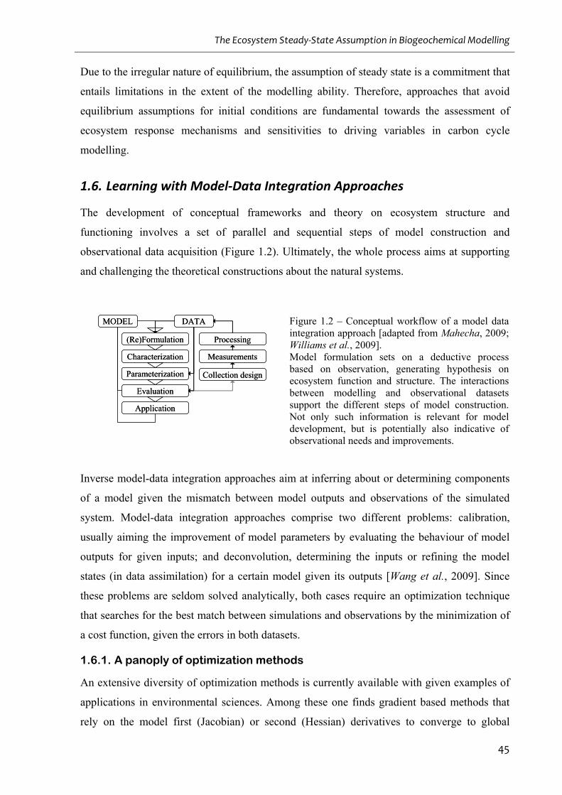
The Ecosystem Steady‐State Assumption in Biogeochemical Modelling
45
Due to the irregular nature of equilibrium, the assumption of steady state is a commitment that
entails limitations in the extent of the modelling ability. Therefore, approaches that avoid
equilibrium assumptions for initial conditions are fundamental towards the assessment of
ecosystem response mechanisms and sensitivities to driving variables in carbon cycle
modelling.
1.6. Learning with Model‐Data Integration Approaches
The development of conceptual frameworks and theory on ecosystem structure and
functioning involves a set of parallel and sequential steps of model construction and
observational data acquisition (Figure 1.2). Ultimately, the whole process aims at supporting
and challenging the theoretical constructions about the natural systems.
Collection design
MODEL DATA
(Re)Formulation
Characterization
Parameterization
Evaluation
Application
Measurements
Processing
Collection design
MODEL DATA
(Re)Formulation
Characterization
Parameterization
Evaluation
Application
Measurements
Processing
Figure 1.2 – Conceptual workflow of a model data integration approach [adapted from Mahecha, 2009; Williams et al., 2009]. Model formulation sets on a deductive process based on observation, generating hypothesis on ecosystem function and structure. The interactions between modelling and observational datasets support the different steps of model construction. Not only such information is relevant for model development, but is potentially also indicative of observational needs and improvements.
Inverse model-data integration approaches aim at inferring about or determining components
of a model given the mismatch between model outputs and observations of the simulated
system. Model-data integration approaches comprise two different problems: calibration,
usually aiming the improvement of model parameters by evaluating the behaviour of model
outputs for given inputs; and deconvolution, determining the inputs or refining the model
states (in data assimilation) for a certain model given its outputs [Wang et al., 2009]. Since
these problems are seldom solved analytically, both cases require an optimization technique
that searches for the best match between simulations and observations by the minimization of
a cost function, given the errors in both datasets.
1.6.1. A panoply of optimization methods
An extensive diversity of optimization methods is currently available with given examples of
applications in environmental sciences. Among these one finds gradient based methods that
rely on the model first (Jacobian) or second (Hessian) derivatives to converge to global
Introduction
46
optima [Byrd et al., 1995; Levenberg, 1944; Marquardt, 1963] and global search methods,
that explore the full spectrum of parameter space within the a priori given parameter ranges
and/or distributions, like Markov chain Monte Carlo approaches [Metropolis et al., 1953].
Inverse optimization is a current active area of research. In addition to the applications of
classic gradient based [e.g. Reichstein et al., 2003b; Santaren et al., 2007] or global search
methods [Wu et al., 2009] arises the development of new search strategies like genetic
algorithms [Barrett, 2002; Deb et al., 2002], multi-objective algorithms [Vrugt et al., 2003]
and adaptive nested algorithms [Vrugt and Robinson, 2007], among others. In general, global
search methods are more robust to ill-posed problems than gradient search methods, but these
are certainly dependent on the specific exercises characteristics (case study, model,
observational datasets and cost function). However, often the high number of model
evaluations required by global search methods becomes impeditive for more complex models
[Santaren et al., 2007].
The available optimization methods can be additionally classified as batch or sequential
approaches, “depending whether the data are processed all at once (batch) or in groups or
possibly even one at a time (sequential)” [Wang et al., 2009]. Usually, batch methods are
associated to calibration [e.g. Knorr and Kattge, 2005] while data assimilation explores
extensively the potential of sequential methods [e.g. Williams et al., 2005]. Despite the
collection of optimization methods, in an optimization inter-comparison study Trudinger et al.
[2007] emphasize the importance of the cost function itself and found no clear distinction in
the success of the optimization neither between gradient based or global search algorithms nor
between batch and sequential methods.
According to Williams et al. [2005], the first applications of data assimilation appear in the
context of filtering and control theory for missile guidance and interception by Maybeck
[1979]. Today, data assimilation is routinely applied to land surface and atmospheric schemes
in support of operational numerical weather prediction activities and model data integration
approaches are frequently used to assess model uncertainties and limitations. Within the scope
of model performance and/or uncertainty assessment, model-data integration approaches aim
at improving the different model components using observations (Figure 1.2).
1.6.2. Improving model-data integration components
In model-data integration approaches the main sources of uncertainty arise from: model
structure, parameters, initial conditions and observational data used in driving or constraining
the model [Liu and Gupta, 2007]. Previous exercises emphasized the role of MDI on the
Learning with Model‐Data Integration Approaches
47
improvements of different components in the framework of ecosystem carbon modelling, e.g.:
selecting superior model structures between ecosystem respiration models [Richardson et al.,
2006a]; selecting parameterizations based on improvements in model performance and
parameter uncertainties including ecophysiology [e.g. Knorr and Kattge, 2005; Santaren et
al., 2007], vegetation [Fox et al., 2009] and soil [Zobitz et al., 2008] turnover rates, soil
carbon transfer rates between pools [Xu et al., 2006] and soil hydraulic properties [Knorr and
Kattge, 2005], among other parameters; estimating the state variables [Williams et al., 2005]
and ecosystem initial conditions [e.g. Braswell et al., 2005; Yeluripati et al., 2009]. In general,
all model-data integration exercises entail the underlying principle of model limits. Models
are built and operated based on assumptions in all its components. And, independently of
model character or complexity, model conceptualization is invariantly based on the
observation of the system. Further assessment of the degree of confidence in the different
model components – individually or as a whole – through observations renders knowledge
about the model and the observed systems.
Additionally, characterizing the statistical distribution of the observational data error is
determinant for the selection of the cost function, e.g.: selecting the ordinary least squares
when the error distribution is normal or the mean absolute error for double exponential error
distributions [Hollinger and Richardson, 2005]. In net ecosystem production measurements,
no consensus arises among recent research since both ordinary least squares [Lasslop et al.,
2008] and mean absolute error [Richardson et al., 2006b] cost functions are equally defended.
More importantly, Lasslop et al. [2008] showed no significant differences in parameter
estimation between both cost functions although parameter uncertainties and root mean square
error of model outputs were higher using the mean absolute error.
1.6.3. Acknowledging equifinality
Equifinality occurs when model realizations with differing model components yield similar
results [Franks et al., 1997]. Within the calibration framework, equifinality seems almost
irrelevant concerning model performance but significantly hampers the distinction of working
hypotheses [Reichstein et al., 2003b]. The fact that varying parameterizations and/or different
model formulations yield similar results and explain equally well observational data does not
contribute to the selection of more appropriate model components and sets an identifiability
issue [Medlyn et al., 2005]. Factors contributing to identifiability include data availability,
model structures, optimization methods, initial values, boundary conditions and parameter
priors [Luo et al., 2009]. More or less explicitly, ecological models need to represent
mechanisms, which often may lead to model complexity and over-parameterization. In over-
Introduction
48
parameterized models, parameters may be correlated and compensate for each other or be
unimportant for model results, which boost parameter uncertainties and/or impede parameter
estimation [Wang et al., 2001]. Moreover, the set of observations used in model development
or evaluation may be limited to distinguish varying modelling representations either due to
data uncertainties [Sorooshian and Gupta, 1983] or to the temporal and/or spatial
characteristics of the dataset [Reichert and Omlin, 1997]. Here, Reichert and Omlin [1997]
make the point that identifiability is a criterion for a good model development and for which
model parsimony is essential but may be a limited approach in assuming model uncertainty
outside the bounds of training sets.
Overall, equifinality limits learning particular dynamics and controls about the systems under
consideration [Franks et al., 1997; Reichstein et al., 2003b]. Moreover, outside the spatial and
temporal domain of the calibration setup the differing model components may yield
significant divergence [Fox et al., 2009] and increase uncertainties in model outputs [Tang
and Zhuang, 2008]. The occurrence of equifinality corroborates the consideration of equally
valid model components in ensemble model runs for a proper quantification of uncertainty in
diagnostic [Beven and Freer, 2001] and prognostic simulations [Tang and Zhuang, 2008].
However, equifinality can be reduced (or avoided?) through the integration of prior
information of model components about the system at hand [Beven and Binley, 1992; Omlin
and Reichert, 1999], which, for example, limit parameters distribution [Van Oijen et al.,
2005]. Also, comparing additional model diagnostics (multiple constraints approaches) often
narrows the parameter spaces that can simultaneously describe several system processes [e.g.
Reichstein et al., 2003b; Williams et al., 2005], hence reducing uncertainties in model
estimates.
1.7. Particularities of the Iberian Peninsula Region
Due to its geographical conditions and historical background the Iberian Peninsula (IP)
presents distinct climate regimes, ecosystem characteristics and bioclimatic patterns.
Recognizing the projected climate variability changes in the IP region and the reduced
attention in evaluating biogeochemical models in Mediterranean ecosystem renders a special
interest in the IP region.
1.7.1. Climatic characteristics
The climatic regimes observed in the Iberian Peninsula are significantly influenced by the air
flows from the surrounding Atlantic Ocean and the Mediterranean Sea. Under the influence of
Particularities of the Iberian Peninsula Region
49
prevailing westerly winds throughout the year, Atlantic cyclones supply most of the rainfall
during the year; except in summer, when their influence is reduced and precipitation is mostly
convective, and rare [Linés Escardó, 1970]. The seasonal precipitation regimes throughout the
year are strongly controlled by synoptic patterns that originate in both water masses and by
the topography distribution [Serrano et al., 1999], showing a strong influence from the North
Atlantic Oscillation (NAO) pattern [Trigo and Palutikof, 2001; Trigo et al., 2004]. According
to Trigo and DaCamara [2000] and Tomás et al. [2004] the Iberian Peninsula is strongly
influenced by ten circulation regimes mostly dominated by the dynamics of the Azores high
pressure systems and inland low pressure systems. In general, the western and central regions
show maximum rainfall between the periods of November and March while the eastern region
shows the two highest precipitation periods in spring and autumn [Rodriguez-Puebla et al.,
1998]. Common throughout Iberia is the extremely low rainfall regime during the warm
summer months [Rodriguez-Puebla et al., 1998], when precipitation shows mostly a local
character [Serrano et al., 1999]. The exceptions are a weak summer precipitation pattern in
the northern Portugal and the Galicia region and the orographic precipitation patterns in the
Cantabrian region [Serrano et al., 1999]. Such patterns imply a strong spatial variability in the
precipitation regime of the Iberian Peninsula: from yearly values between 250 and 1900 mm
[Mitchell et al., 2004]. Between 1951 and 2002 it is observed a general reduction in daily
rainfall intensity; decreasing patterns in total precipitation were observed for northern and
southern regions during winter periods and in some southern regions in spring [Rodrigo and
Trigo, 2007]. A predominant decrease in seasonal and annual precipitation in the
Mediterranean Iberian Peninsula in second half of 20th century was also observed by De Luis
et al. [2009].
The temperature regime in the IP can be characterized by relatively mild temperatures in
winter and fairly hot in summer. The spatial distribution is mainly controlled by topography
and continentality [Linés Escardó, 1970] and shows significant latitudinal and altitudinal
gradients [e.g. Gallardo et al., 2001]. Relatively warm mean annual temperatures are
observed throughout the IP, between 9 and 18ºC [Mitchell et al., 2004], except in very high
altitudes [Linés Escardó, 1970]. The hottest months are July and August, in the interior and
coastal areas, respectively, while the lowest temperatures are usually observed January, under
the influence of the European continental high pressure system [Linés Escardó, 1970]. Spring
and autumn temperatures are usually warm, showing a seasonal average around 8 to 17ºC
[Mitchell et al., 2004]. Summer periods are characterized by the occurrence of thermal lows
over the IP, comprising a dominant weather regime that characterizes the hot and dry
Introduction
50
summers of Mediterranean Iberia [Linés Escardó, 1970; Martin et al., 2001]. Both minimum
and maximum (more marked) temperatures series show increases since the 1970’s [Esteban-
Parra et al., 2003]. Further, inter-annual variation of winter temperatures are significantly
associated to NAO patterns, based on the indirect effect of nebulosity on maximum and
minimum temperatures, through daytime changes in the incoming solar radiation and night-
time decreases in outgoing long wave radiation, respectively [Esteban-Parra et al., 2003;
Trigo et al., 2002]. The high temperature amplitudes observed in southern IP [Linés Escardó,
1970] place it amongst the regions of higher temperature amplitudes in the world [Aires and
Prigent, 2006].
In general, the air clarity over the IP is such that ground level solar radiation measurements
are usually very high. The maximum transparencies in the atmosphere are observed in the
spring, due to the advection of cold air masses over actively heated ground. Further, the IP is
one of the most highly insulated areas of Europe, with an average of 2500 hours of sunshine
per year, having south-western maximum and north-eastern minimum values [Linés Escardó,
1970]. The lowest precipitation season – hence lowest nebulosity – coincides with the longest
day length and higher sun angle periods of the year, hence highest solar radiation periods. The
spatial variability can be classified in four distinct sub-regions (north, south, west, east) that
exhibit different annual and seasonal trends between 1951 and 2004 [Sanchez-Lorenzo et al.,
2007]. For the IP region, from the 1950s until the 1980s, Sanchez-Lorenzo et al. [2007] found
a decreasing trend in sunshine duration, followed by an increase until the end of the 20th
century. The NAO patterns contribute significantly to the inter-annual variability in solar
radiation of the Iberian Peninsula [Jones et al., 1997], where a positive increment in monthly
sunshine duration (10% to 20%) can be expected during the positive phase of the NAO [Pozo-
Vazquez et al., 2004].
Overall, the climate regimes of the Iberian Peninsula are translated by dry hot summers and
wetter mild winters in most of the Mediterranean region. The limiting factors for vegetation
development change between the water limited periods of hot and sunny summers and the
temperature limited winters, when water availability is more abundant. Further, summer
droughts are frequent and originate from seasonal prolonged high temperature and low
precipitation periods. But the strong existing latitudinal and altitudinal gradients enable the
presence of northern and higher regions where summer water stresses are less prone to occur.
These spatial and seasonal patterns strongly shape the ecosystems’ function, diversity and
distribution patterns in the IP region.
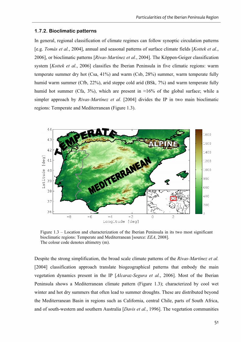
Particularities of the Iberian Peninsula Region
51
1.7.2. Bioclimatic patterns
In general, regional classification of climate regimes can follow synoptic circulation patterns
[e.g. Tomás et al., 2004], annual and seasonal patterns of surface climate fields [Kottek et al.,
2006], or bioclimatic patterns [Rivas-Martínez et al., 2004]. The Köppen-Geiger classification
system [Kottek et al., 2006] classifies the Iberian Peninsula in five climatic regions: warm
temperate summer dry hot (Csa, 41%) and warm (Csb, 28%) summer, warm temperate fully
humid warm summer (Cfb, 22%), arid steppe cold arid (BSk, 7%) and warm temperate fully
humid hot summer (Cfa, 3%), which are present in ≈16% of the global surface; while a
simpler approach by Rivas-Martínez et al. [2004] divides the IP in two main bioclimatic
regions: Temperate and Mediterranean (Figure 1.3).
Figure 1.3 – Location and characterization of the Iberian Peninsula in its two most significant bioclimatic regions: Temperate and Mediterranean [source: EEA, 2008]. The colour code denotes altimetry (m).
Despite the strong simplification, the broad scale climate patterns of the Rivas-Martínez et al.
[2004] classification approach translate biogeographical patterns that embody the main
vegetation dynamics present in the IP [Alcaraz-Segura et al., 2006]. Most of the Iberian
Peninsula shows a Mediterranean climate pattern (Figure 1.3); characterized by cool wet
winter and hot dry summers that often lead to summer droughts. These are distributed beyond
the Mediterranean Basin in regions such as California, central Chile, parts of South Africa,
and of south-western and southern Australia [Davis et al., 1996]. The vegetation communities
Introduction
52
of these regions share structural and functional characteristics that have to cope with scarce
and unpredictable water availability during the summer warmer periods and with cooler
temperatures during the wet winters, limiting the favourable growing season to short periods
in spring and autumn.
1.7.3. Mediterranean ecosystems
The panoply of different controls on photosynthesis and growth upon drought tends to shape
community composition in drought prone regions [Chaves et al., 2002]. In Mediterranean
areas, precipitation or water availability represents the general limiting factor to vegetation
development and is reflected in different structural and functional aspects of vegetation
behaviour, namely on: the superior predictive power of water balance derived indexes to
explain spatial vegetation distribution patterns [Gavilan, 2005]; the stronger dependence on
precipitation than on temperature of coastal shrub flowering [Prieto et al., 2008]; changes in
rooting depth [Canadell et al., 1996] and horizontal distribution patterns [Moreno et al.,
2005]; midday stomatal closure limiting water loss during maximum evaporative demands
[Tenhunen et al., 1987]; changes in leaf area index, reducing surface area in lower
precipitation regions [Joffre et al., 2007] or other morphological adaptations, such as
sclerophylly [Turner, 1994]; changes in carbon allocation strategies, investing in resource
storage in stems, increasing root lengths and reducing leaf area [Rodrigues et al., 1995]; as
well as other different water-use strategies to overcome the strong dry summer [Chaves et al.,
2002; David et al., 2007]; and on the inter-annual variability in phenological activity [Gouveia
et al., 2008; Vicente-Serrano and Heredia-Laclaustra, 2004]. In this regard, recent studies
have shown that the inter-annual variability in winter precipitation over the IP is strongly
influenced by the North Atlantic Oscillation (NAO), consequently impacting the vegetation
activity of the following year: positive (negative) winter NAO bring reduced (increased)
winter precipitation regimes inducing low (high) vegetation activity in the following spring
and summer seasons. Additionally, allocation strategies for primary shoot growth can be
strongly driven by the unpredictability of resource availability, which would partly explain
phenological diversity of Mediterranean woody vegetation [Castro-Diez et al., 2003]. Despite
particular climate characteristics of Mediterranean regions, Joffre et al. [2007] highlight the
limitations and the current discussions about plant adaptation and differentiation in terms of
morphology, ecophysiology or trait convergence in Mediterranean ecosystems. Overall, leaf
level observations of photosynthetic rates of Mediterranean species do not appear to
significantly differ from other biome species [Damesin et al., 1998; Joffre et al., 1999],
despite needing to manage the excessive interception of solar radiation through
Particularities of the Iberian Peninsula Region
53
photoprotection mechanisms when summer low water availability and high temperatures
occur [e.g. Demmig-Adams et al., 1989].
The diversity of Mediterranean ecosystems cannot be exclusively explained by climate
factors, despite its strong controls on vegetation spatial and temporal dynamics. The human
occupation of the Mediterranean Basin can be traced back to the early Holocene with
significant consequences to the ecosystems biodiversity, structural and functional levels
[Blondel, 2006]. For example, the role of human management is responsible for a high
resistance of the Mediterranean Basin to plant invasive species, but human induced changes
here have also contributed to increases in biodiversity through balanced grazing [Blondel,
2006]. An important result from the long term human influence in the Mediterranean Basin
landscape was the formation of savannah-like systems designated by montados (Portugal) or
dehesas (Spain) that are dominated by scattered evergreen oak woodlands with open and
heterogeneous canopies with shrub and annual herbaceous understories [Joffre et al., 1999].
These consist of mixed agroforestry systems of important socio-economic value at local and
national levels that rely mainly on the exploration of cork, wood and acorn, from cork and
holm oak trees, respectively, while herbaceous layer may consist of cereal crops (oats, barley,
wheat) or native annual species for grazing [Joffre and Rambal, 2006]. Nowadays, the
extensive animal production contributes significantly to the economic sustainability of these
agroforestry systems [Gaspar et al., 2007]. The human-induced changes in land-use and
resources management add a human dimension to the abiotic controls on the montado’s
spatial and temporal dynamics [Costa et al., 2009], which significantly shaped the three-
dimensional architecture of these ecosystems. In these water and nutrient availability limited
regions, the presence of scattered trees increases locally the water holding capacity and the
nutrient availability, which significantly influences the spatial distribution of species richness
at the landscape level [Joffre et al., 1999; Joffre and Rambal, 2006]. The extensive character
of human occupation provides a long term ecological sustainability to these Mediterranean
systems, which can be disrupted through intensification practices [Joffre et al., 1999] or land
abandonment. For instance, landscape patchiness found in southern Portugal following land
abandonment is a significant precursor of desertification [Seixas, 2000]. Modelling results
show that land degradation impacts the Iberian climate regimes locally and regionally,
including general increases in surface temperature (proportional to increases in bare ground
fraction) and reductions in summer precipitation in Mediterranean regions of the IP (mostly in
the north-eastern areas) [Arribas et al., 2003]. The recent association between late spring early
summer Mediterranean drought and summer temperature increases in temperate continental
Introduction
54
Europe emphasizes the role of Mediterranean ecosystem dynamics at wider regional spatial
scales [Zampieri et al., 2009].
Additionally, fire is a common perturbation mechanism in Mediterranean ecosystems that
shapes vegetation composition and ecosystem structure. At the landscape and local scale, the
fire frequency, extent and spatial distribution exerts controls on the abundance and richness
spatial distribution of different plant functional types depending on strategies to cope with
varying fire regimes, for instance: increases in fire frequency support the development of
seeders (instead of resprouters) in shrub communities, but not for very high frequencies; while
the abundance of tree seeders is reduced with higher fire frequencies since the time between
fire events becomes too short to allow the development of new cohorts [Pausas and Lloret,
2007]. Consequently, trends in fire frequency can yield significant changes in species richness
at local scales [Pausas and Lloret, 2007], for instance, increasing fire recurrence has driven
declines in Pinus halepensis populations and increasing shrub abundance [Eugenio and
Lloret, 2004] and is shown to inhibit the regenerative process of Q. suber populations [Acácio
et al., 2009]; but given favourable conditions in the early stages of regeneration, the combined
effects of increasing fire frequency and land abandonment processes may facilitate the
expansion of Q. suber populations [Pons and Pausas, 2006]. Additionally, Pausas et al.
[2003] also observed lower mortality and higher growth due to better soil fertility resulting
from post-fire higher SOM mineralization and hash deposition in higher severity burned areas.
However, fire severity can also be a precursor of increasing soil erosion and consequent
export of hash materials.
1.7.4. Vulnerabilities within the context future climate scenarios
The Mediterranean Basin is considered one of the significant hot-spots in the context of future
climate scenarios, where decreases in summer (~22%) and winter (~10%) precipitation are
expected, as well as increases in its inter-annual variability of 25% and 40%, respectively
[Giorgi, 2006]. The projected changes in Mediterranean region temperatures are also higher
than the global average temperature changes [Giorgi, 2006] especially in summer periods,
potentially exceeding 6ºC over the IP region [Christensen and Christensen, 2007]. These
trends suggest increases in the frequency of climate summer drought or extreme rainfall
episodes in Mediterranean regions. Additionally, the projected increases in summer
temperature (~15%, [Giorgi, 2006]) and precipitation inter-annual variability are prone to
strengthen the intensity of climate extremes, like summer droughts. The projected changes in
climate regimes entail implications for the distribution patterns of vegetation, e.g., individual
and community level impacts of drought on particular species [e.g. Pinus silvestris, Martinez-
Particularities of the Iberian Peninsula Region
55
Vilalta and Pinol, 2002] would tend to show a rapid population decrease in the more affected
central and southern regions of the IP [Garzon et al., 2008]; and future increases in Iberian
summer dry spells would tend to increase desertification and wildfire processes [Hoinka et al.,
2007]. According to the work of Zampieri et al. [2009] the implications of temperature
increases can span beyond the geographical domain of Mediterranean regions. Furthermore, if
not embedded in the climate projections already, these phenomena could emphasize future
effects on climate variability. The importance of regionally focused approaches stems from
limits in coherent projections of ecosystem behaviour [Friedlingstein et al., 2006] and from
acknowledging the spatial heterogeneity of climate variability and carbon cycle response to
environmental changes [Ito, 2005]. Hence, regional studies can yield significant results with
implications outside its domain as well as provide valuable information about the limits of
more general approaches.
1.8. Research Scope and Objectives
Biogeochemical models embed representations of the fundamental and general dynamics of
ecosystem functioning, which contributes to their wide application from local to global scales
in the context of the terrestrial carbon cycle research. Model development often aims at
comprehensiveness and builds on different conceptual and practical strategies, which depend
on its application framework. However, the limited information on ecosystem carbon pools
leads to standard assumptions of equilibrium conditions in model initialization routines,
entailing a structural limitation in modelling exercises. The present research aims to quantify
the impacts of the steady-state assumption in modelling the carbon fluxes of terrestrial
ecosystems, from local to regional scales; and proposes methods to minimize its effect in
modelled net ecosystem fluxes, following a bottom-up approach. The implications of initial
equilibrium conditions are investigated from inverse model parameter optimizations at site
level to regional forward model simulations.
The paradigm of model-data integration is adopted to support the overall research. The
existing modelling approaches stand on a more or less substantial set of observational data
streams. In this regard, production efficiency models, in addition to climate data, integrate
time series of remotely sensed vegetation biophysical properties, exchanging model
complexity by prescribed vegetation dynamics that increase model spatial representativeness.
Observational strategies aim at a better process understanding, as well as to improve the
ability of model structures to quantify terrestrial ecosystem carbon fluxes. Throughout the
Introduction
56
work presented here, different data streams are exploited in the context of production
efficiency model.
The input data dependencies of production efficiency models provide an ideal modelling
framework to integrate in situ observations of net ecosystem fluxes and meteorological
measurements with remotely sensing data of vegetation biophysical properties. Eddy-
covariance measurements and the emergence of the FLUXNET database provide unique
observations of ecosystem-atmosphere carbon fluxes. Here, confronting in situ observations
with simulations of net ecosystem production fluxes aims at addressing the issue of
confidence in the performance of particular modelling structures as well as to question the
impacts of the general steady-state assumption on parameter retrievals and modelling
uncertainty. But several historical dynamics can similarly lead to disequilibrium conditions.
Exploring the feasibility or likelihood of different scenarios and structural approaches –
empirical or more mechanistic – represents a useful modelling exercise. In this context, the
contribution of model-data integration approaches aims at distinguishing the ability of
different modelling structures in prescribing nonequilibrium conditions.
Most TBMs encompass a broad-spectrum of applications with a limited treatment of specific
ecosystem functions. Here, understanding the models’ ability to simulate carbon fluxes locally
for different ecosystem types is regionally relevant. In this regard, the extended set of eddy-
covariance sites optimized aims to improve its regional representativeness. The site level
optimizations encompass various plant functional types as well as different phenology and
climate regimes. Following a bottom-up work flow, such results contribute with knowledge
on the different modelling components to the regional simulation exercises. However, as
referred above, several issues hamper a proper description of initial conditions at regional
scales. Hence, an additional goal comprises the evaluation of the impacts of the steady-state
assumption on the inter-annual variability and temporal trends of modelled fluxes, as well as a
proposal of a methodology to minimize such effects.
The Iberian Peninsula constitutes an interesting region to evaluate TBMs for its
Mediterranean characteristics and for the prospective changes in climate conditions of the
Mediterranean basin. Further, modelling results show a high inter-annual variability in net
ecosystem production fluxes in the Iberian Peninsula [Potter et al., 2005], which encourage
selecting the Iberian Peninsula as a case study.
Ultimately, the main questions driving the current research can be stated as:
Research Scope and Objectives
57
1. What are the implications of initial equilibrium assumptions on inverse model
optimization approaches?
2. How can equilibrium assumptions – or the impact of equilibrium assumptions – be
avoided from local to regional scales?
3. Can Mediterranean – more particularly Iberian – ecosystems be represented by
terrestrial biogeochemical models? And, in this regard, which are the dynamics
underlying the inter-annual variability and temporal trends in net ecosystem
production estimates?
The current research approach stands on the concept that model-data integration approaches
are relevant towards a comprehensive understanding of the natural and modelling systems.
Modelling exercises embodying flexible structures are instrumental in recognizing conceptual
limitations or alternative hypothesis of ecosystem function.
1.9. Structure of the Dissertation
The present dissertation is divided in three main chapters, translating the strategy followed to
investigate the general implications of the ecosystem steady-state assumption in modelling
exercises. The ability of terrestrial biogeochemical models to simulate net ecosystem
production fluxes in the Iberian Peninsula emerges from the emphasis given to modelling
Mediterranean systems throughout the different chapters.
Following a model-data integration approach for inverse parameter optimization, the impacts
of the general steady-state assumption on parameter retrievals and modelling uncertainty are
investigated in Chapter 2. The production efficiency model CASA [Carnegie Ames Stanford
Approach, Potter et al., 1993] is introduced. An additional parameter, η, which relaxes the
initial steady-state assumption in the soil carbon pools, is incorporated in the optimized
parameter vector. The biases and higher uncertainties in model parameters that govern the
responses of NPP and RH to environmental drivers are addressed.
As can be rightly posed, the prior heuristic approach (η) is unable to address the hypothesis of
nonequilibrium conditions in vegetation carbon pools, mainly wood. In Chapter 3
nonequilibrium conditions are investigated in both vegetation and soil carbon pools, following
both empirical and more mechanistic modelling approaches. Equifinality issues are addressed
by constraining model outputs of carbon fluxes and pools in multiple constraints approach
framework.
Introduction
58
In Chapter 4, the set of eddy-covariance sites used for inverse model optimization is
significantly extended, mainly aiming at a better representation of ecosystems in the Iberian
Peninsula. A method to evaluate inter-annual variability and temporal trends in net ecosystem
fluxes solely driven by dynamic forcing, quasi independently from the initial conditions, is
proposed. The ecosystem processes underlying the NEP dynamics in the Iberian Peninsula
between 1982 and 2006 are investigated within the CASA modelling framework.
Concluding remarks on the steady-state-driven limitations in bottom-up biogeochemical
modelling approaches in the context of the terrestrial component of the carbon cycle are
synthesized in Chapter 5.
The materials of the three chapters corresponding to different modelling exercises are
published (Chapter 2), accepted for publication (Chapter 3) and submitted (Chapter 4) in peer
reviewed journals. The appendices reflect additional materials in the context of the
publications themselves.
References
Aber, J., W. McDowell, K. Nadelhoffer, A. Magill, G. Berntson, M. Kamakea, S. McNulty, W. Currie, L. Rustad, and I. Fernandez (1998), Nitrogen saturation in temperate forest ecosystems - Hypotheses revisited, Bioscience, 48(11), 921-934.
Abramowitz, G. (2005), Towards a benchmark for land surface models, Geophys Res Lett, 32(22), doi:10.1029/2005GL024419
Abramowitz, G., H. Gupta, A. Pitman, Y. P. Wang, R. Leuning, H. Cleugh, and K. L. Hsu (2006), Neural error regression diagnosis (NERD): A tool for model bias identification and prognostic data assimilation, J Hydrometeorol, 7(1), 160-177.
Acácio, V., M. Holmgren, F. Rego, F. Moreira, and G. M. J. Mohren (2009), Are drought and wildfires turning Mediterranean cork oak forests into persistent shrublands?, Agroforest Syst, 76(2), 389-400.
Ainsworth, E. A., and A. Rogers (2007), The response of photosynthesis and stomatal conductance to rising [CO2]: mechanisms and environmental interactions, Plant Cell Environ, 30(3), 258-270.
Aires, F., and C. Prigent (2006), Toward a new generation of satellite surface products?, J Geophys Res-Atmos, 111(D22), doi:10.1029/2006JD007362.
Alcaraz-Segura, D., J. Paruelo, and J. Cabello (2006), Identification of current ecosystem functional types in the Iberian Peninsula, Global Ecol Biogeogr, 15(2), 200-212.
Amthor, J. S. (2000), The McCree-de Wit-Penning de Vries-Thornley respiration paradigms: 30 years later, Ann Bot-London, 86(1), 1-20.
Archer, D. (1995), Upper Ocean Physics as Relevant to Ecosystem Dynamics - a Tutorial, Ecol Appl, 5(3), 724-739.
Arrhenius, S. (1896), On the Influence of Carbonic Acid in the Air upon the Temperature of the Ground, Philosophical Magazine and Journal of Science, 41, 237-276.
References
59
Arrhenius, S. (1898), The effect of constant influences upon physiological relationships, Scandinavian Archives of Physiology(8), 367-415.
Arribas, A., C. Gallardo, M. A. Gaertner, and M. Castro (2003), Sensitivity of the Iberian Peninsula climate to a land degradation, Clim Dynam, 20(5), 477-489.
Asrar, G., R. B. Myneni, and B. J. Choudhury (1992), Spatial Heterogeneity in Vegetation Canopies and Remote-Sensing of Absorbed Photosynthetically Active Radiation - a Modeling Study, Remote Sens Environ, 41(2-3), 85-103.
Aubinet, M., A. Grelle, A. Ibrom, U. Rannik, J. Moncrieff, T. Foken, A. S. Kowalski, P. H. Martin, P. Berbigier, C. Bernhofer, R. Clement, J. Elbers, A. Granier, T. Grunwald, K. Morgenstern, K. Pilegaard, C. Rebmann, W. Snijders, R. Valentini, and T. Vesala (2000a), Estimates of the annual net carbon and water exchange of forests: The EUROFLUX methodology, Adv Ecol Res, 30, 113-175.
Aubinet, M., A. Grelle, A. Ibrom, U. Rannik, J. Moncrieff, T. Foken, A. S. Kowalski, P. H. Martin, P. Berbigier, C. Bernhofer, R. Clement, J. Elbers, A. Granier, T. Grunwald, K. Morgenstern, K. Pilegaard, C. Rebmann, W. Snijders, R. Valentini, and T. Vesala (2000b), Estimates of the annual net carbon and water exchange of forests: The EUROFLUX methodology, Advances in Ecological Research, 30, 113-175.
Aubinet, M., B. Chermanne, M. Vandenhaute, B. Longdoz, M. Yernaux, and E. Laitat (2001), Long term carbon dioxide exchange above a mixed forest in the Belgian Ardennes, Agr Forest Meteorol, 108(4), 293-315.
Aubinet, M., B. Heinesch, and B. Longdoz (2002), Estimation of the carbon sequestration by a heterogeneous forest: night flux corrections, heterogeneity of the site and inter-annual variability, Global Change Biol, 8(11), 1053-1071.
Aubinet, M., R. Clement, J. A. Elbers, T. Foken, A. Grelle, A. Ibrom, J. Moncrieff, K. Pilegaard, Ü. Rannik, and C. Rebmann (2003), Methodology for data acquisition, storage and treatment, in Fluxes of carbon, water, and energy of European forests, edited by R. Valentini, Springer, Berlin ; New York.
Aubinet, M., P. Berbigier, C. H. Bernhofer, A. Cescatti, C. Feigenwinter, A. Granier, T. H. Grunwald, K. Havrankova, B. Heinesch, B. Longdoz, B. Marcolla, L. Montagnani, and P. Sedlak (2005), Comparing CO2 storage and advection conditions at night at different carboeuroflux sites, Bound-Lay Meteorol, 116(1), 63-94.
Austin, A. T., R. W. Howarth, J. S. Baron, F. S. C. III, T. R. Christensen, E. A. Holland, M. V. Ivanov, A. Y. Lein, L. A. Martinelli, J. M. Melillo, and C. Shang (2003), Human disruption of element interactions: drivers, consequences, and trends for the twenty-first century, in Interactions of the major biogeochemical cycles: global change and human impacts, edited by J. M. Melillo, et al., pp. xxi, 357 p., Island Press, Washington.
Ayres, M. P., and M. J. Lombardero (2000), Assessing the consequences of global change for forest disturbance from herbivores and pathogens, Sci Total Environ, 262(3), 263-286.
Bacour, C., F. Baret, D. Beal, M. Weiss, and K. Pavageau (2006), Neural network estimation of LAI, fAPAR, fCover and LAIxC(ab), from top of canopy MERIS reflectance data: Principles and validation, Remote Sens Environ, 105(4), 313-325.
Baldocchi, D. (2008), Breathing of the terrestrial biosphere: lessons learned from a global network of carbon dioxide flux measurement systems, Aust J Bot, 56(1), 1-26.
Baldocchi, D. D., B. B. Hicks, and T. P. Meyers (1988), Measuring Biosphere-Atmosphere Exchanges of Biologically Related Gases with Micrometeorological Methods, Ecology, 69(5), 1331-1340.
Introduction
60
Baldocchi, D. D. (2003), Assessing the eddy covariance technique for evaluating carbon dioxide exchange rates of ecosystems: past, present and future, Global Change Biol, 9(4), 479-492.
Baret, F., O. Hagolle, B. Geiger, P. Bicheron, B. Miras, M. Huc, B. Berthelot, F. Nino, M. Weiss, O. Samain, J. L. Roujean, and M. Leroy (2007), LAI, fAPAR and fCover CYCLOPES global products derived from VEGETATION - Part 1: Principles of the algorithm, Remote Sens Environ, 110(3), 275-286.
Barrett, D. J. (2002), Steady state turnover time of carbon in the Australian terrestrial biosphere, Global Biogeochem Cy, 16(4).
Berg, B., G. Ekbohm, M. B. Johansson, C. McClaugherty, F. Rutigliano, and A. V. DeSanto (1996), Maximum decomposition limits of forest litter types: A synthesis, Can J Bot, 74(5), 659-672.
Berg, B., C. McClaugherty, A. V. De Santo, and D. Johnson (2001), Humus buildup in boreal forests: effects of litter fall and its N concentration, Can J Forest Res, 31(6), 988-998.
Berry, J., and O. Bjorkman (1980), Photosynthetic Response and Adaptation to Temperature in Higher-Plants, Annu Rev Plant Phys, 31, 491-543.
Berthelot, M., P. Friedlingstein, P. Ciais, J. L. Dufresne, and P. Monfray (2005), How uncertainties in future climate change predictions translate into future terrestrial carbon fluxes, Global Change Biol, 11(6), 959-970.
Beven, K., and A. Binley (1992), The Future of Distributed Models - Model Calibration and Uncertainty Prediction, Hydrol Process, 6(3), 279-298.
Beven, K., and J. Freer (2001), Equifinality, data assimilation, and uncertainty estimation in mechanistic modelling of complex environmental systems using the GLUE methodology, J Hydrol, 249(1-4), 11-29.
Blain, S., B. Queguiner, L. Armand, S. Belviso, B. Bombled, L. Bopp, A. Bowie, C. Brunet, C. Brussaard, F. Carlotti, U. Christaki, A. Corbiere, I. Durand, F. Ebersbach, J. L. Fuda, N. Garcia, L. Gerringa, B. Griffiths, C. Guigue, C. Guillerm, S. Jacquet, C. Jeandel, P. Laan, D. Lefevre, C. Lo Monaco, A. Malits, J. Mosseri, I. Obernosterer, Y. H. Park, M. Picheral, P. Pondaven, T. Remenyi, V. Sandroni, G. Sarthou, N. Savoye, L. Scouarnec, M. Souhaut, D. Thuiller, K. Timmermans, T. Trull, J. Uitz, P. van Beek, M. Veldhuis, D. Vincent, E. Viollier, L. Vong, and T. Wagener (2007), Effect of natural iron fertilization on carbon sequestration in the Southern Ocean, Nature, 446(7139), 1070-U1071.
Blondel, J. (2006), The 'Design' of mediterranean landscapes: A millennial story of humans and ecological systems during the historic period, Human Ecology, 34(5), 713-729.
Bolker, B. M., S. W. Pacala, and W. J. Parton (1998), Linear analysis of soil decomposition: Insights from the century model, Ecol Appl, 8(2), 425-439.
Bonan, G. B. (2002), Ecological climatology : concepts and applications, xi, 678 p. pp., Cambridge University Press, New York.
Bonan, G. B. (2008), Forests and Climate Change: Forcings, Feedbacks, and the Climate Benefits of Forests, Science, 320(5882), 1444-1449.
Bondeau, A., P. C. Smith, S. Zaehle, S. Schaphoff, W. Lucht, W. Cramer, and D. Gerten (2007), Modelling the role of agriculture for the 20th century global terrestrial carbon balance, Global Change Biol, 13(3), 679-706.
Botkin, D. B., J. R. Wallis, and J. F. Janak (1972), Some Ecological Consequences of a Computer Model of Forest Growth, J Ecol, 60(3), 849-872.
References
61
Box, E. O. (1981), Predicting Physiognomic Vegetation Types with Climate Variables, Vegetatio, 45(2), 127-139.
Braswell, B. H., W. J. Sacks, E. Linder, and D. S. Schimel (2005), Estimating diurnal to annual ecosystem parameters by synthesis of a carbon flux model with eddy covariance net ecosystem exchange observations, Global Change Biol, 11(2), 335-355.
Brown, S. L., and P. E. Schroeder (1999), Spatial patterns of aboveground production and mortality of woody biomass for eastern US forests, Ecol Appl, 9(3), 968-980.
Brzeziecki, B., F. Kienast, and O. Wildi (1993), A Simulated Map of the Potential Natural Forest Vegetation of Switzerland, J Veg Sci, 4(4), 499-508.
Buermann, W., S. Saatchi, T. B. Smith, B. R. Zutta, J. A. Chaves, B. Mila, and C. H. Graham (2008), Predicting species distributions across the Amazonian and Andean regions using remote sensing data, J Biogeogr, 35(7), 1160-1176.
Bugmann, H. (2001), A review of forest gap models, Climatic Change, 51(3-4), 259-305.
Burnham, K. P., and D. R. Anderson (2004), Multimodel inference - understanding AIC and BIC in model selection, Sociological Methods & Research, 33(2), 261-304.
Byrd, R. H., P. H. Lu, J. Nocedal, and C. Y. Zhu (1995), A Limited Memory Algorithm for Bound Constrained Optimization, Siam J Sci Comput, 16(5), 1190-1208.
Cairns, M. A., S. Brown, E. H. Helmer, and G. A. Baumgardner (1997), Root biomass allocation in the world's upland forests, Oecologia, 111(1), 1-11.
Canadell, J., R. B. Jackson, J. R. Ehleringer, H. A. Mooney, O. E. Sala, and E. D. Schulze (1996), Maximum rooting depth of vegetation types at the global scale, Oecologia, 108(4), 583-595.
Canadell, J., D. Pataki, R. Gifford, R. Houghton, Y. Lou, M. Raupach, P. Smith, and W. Steffen (2007a), Saturation of the terrestrial carbon sink in Terrestrial ecosystems in a changing world, edited by J. G. Canadell, et al., Springer, Berlin ; New York.
Canadell, J. G., C. Le Quere, M. R. Raupach, C. B. Field, E. T. Buitenhuis, P. Ciais, T. J. Conway, N. P. Gillett, R. A. Houghton, and G. Marland (2007b), Contributions to accelerating atmospheric CO2 growth from economic activity, carbon intensity, and efficiency of natural sinks, P Natl Acad Sci USA, 104(47), 18866-18870.
Castro-Diez, P., G. Montserrat-Marti, and J. H. C. Cornelissen (2003), Trade-offs between phenology, relative growth rate, life form and seed mass among 22 Mediterranean woody species, Plant Ecol, 166(1), 117-129.
Ceccato, P., S. Flasse, S. Tarantola, S. Jacquemoud, and J. M. Gregoire (2001), Detecting vegetation leaf water content using reflectance in the optical domain, Remote Sens Environ, 77(1), 22-33.
Chambers, J. Q., J. I. Fisher, H. C. Zeng, E. L. Chapman, D. B. Baker, and G. C. Hurtt (2007), Hurricane Katrina's carbon footprint on U. S. Gulf Coast forests, Science, 318(5853), 1107-1107.
Chapin, F. S., G. R. Shaver, A. E. Giblin, K. J. Nadelhoffer, and J. A. Laundre (1995), Responses of Arctic Tundra to Experimental and Observed Changes in Climate, Ecology, 76(3), 694-711.
Chatterjee, A., R. Lal, L. Wielopolski, M. Z. Martin, and M. H. Ebinger (2009), Evaluation of Different Soil Carbon Determination Methods, Crit. Rev. Plant Sci., 28(3), 164-178.
Introduction
62
Chaves, M. M., J. S. Pereira, J. Maroco, M. L. Rodrigues, C. P. P. Ricardo, M. L. Osorio, I. Carvalho, T. Faria, and C. Pinheiro (2002), How Plants Cope with Water Stress in the Field? Photosynthesis and Growth, edited, pp. 907-916.
Chen, J., P. Jonsson, M. Tamura, Z. H. Gu, B. Matsushita, and L. Eklundh (2004), A simple method for reconstructing a high-quality NDVI time-series data set based on the Savitzky-Golay filter, Remote Sens Environ, 91(3-4), 332-344.
Christensen, J. H., and O. B. Christensen (2007), A summary of the PRUDENCE model projections of changes in European climate by the end of this century, Climatic Change, 81, 7-30.
Ciais, P., M. Reichstein, N. Viovy, A. Granier, J. Ogee, V. Allard, M. Aubinet, N. Buchmann, C. Bernhofer, A. Carrara, F. Chevallier, N. De Noblet, A. D. Friend, P. Friedlingstein, T. Grunwald, B. Heinesch, P. Keronen, A. Knohl, G. Krinner, D. Loustau, G. Manca, G. Matteucci, F. Miglietta, J. M. Ourcival, D. Papale, K. Pilegaard, S. Rambal, G. Seufert, J. F. Soussana, M. J. Sanz, E. D. Schulze, T. Vesala, and R. Valentini (2005), Europe-wide reduction in primary productivity caused by the heat and drought in 2003, Nature, 437(7058), 529-533.
Collatz, G. J., J. T. Ball, C. Grivet, and J. A. Berry (1991), Physiological and Environmental-Regulation of Stomatal Conductance, Photosynthesis and Transpiration - a Model That Includes a Laminar Boundary-Layer, Agr Forest Meteorol, 54(2-4), 107-136.
Collatz, G. J., M. Ribas-Carbo, and J. A. Berry (1992), Coupled Photosynthesis-Stomatal Conductance Model for Leaves of C4 Plants, Aust J Plant Physiol, 19(5), 519-538.
Costa, A., H. Pereira, and M. Madeira (2009), Landscape dynamics in endangered cork oak woodlands in Southwestern Portugal (1958-2005), Agroforest Syst, 77(2), 83-96.
Cramer, W., D. W. Kicklighter, A. Bondeau, B. Moore, C. Churkina, B. Nemry, A. Ruimy, A. L. Schloss, and P. P. N. M. Intercompariso (1999), Comparing global models of terrestrial net primary productivity (NPP): overview and key results, Global Change Biol, 5, 1-15.
Cramer, W., A. Bondeau, F. I. Woodward, I. C. Prentice, R. A. Betts, V. Brovkin, P. M. Cox, V. Fisher, J. A. Foley, A. D. Friend, C. Kucharik, M. R. Lomas, N. Ramankutty, S. Sitch, B. Smith, A. White, and C. Young-Molling (2001), Global response of terrestrial ecosystem structure and function to CO2 and climate change: results from six dynamic global vegetation models, Global Change Biol, 7(4), 357-373.
Crout, N. M. J., D. Tarsitano, and A. T. Wood (2009), Is my model too complex? Evaluating model formulation using model reduction, Environmental Modelling & Software, 24(1), 1-7.
Curiel Yuste, J., D. D. Baldocchi, A. Gershenson, A. Goldstein, L. Misson, and S. Wong (2007), Microbial soil respiration and its dependency on carbon inputs, soil temperature and moisture, Global Change Biol, 13(9), 2018-2035.
Damesin, C., S. Rambal, and R. Joffre (1998), Co-occurrence of trees with different leaf habit: a functional approach on Mediterranean oaks, Acta Oecol, 19(3), 195-204.
David, T. S., M. O. Henriques, C. Kurz-Besson, J. Nunes, F. Valente, M. Vaz, J. S. Pereira, R. Siegwolf, M. M. Chaves, L. C. Gazarini, and J. S. David (2007), Water-use strategies in two co-occurring Mediterranean evergreen oaks: surviving the summer drought, Tree Physiol, 27(6), 793-803.
Davidson, E. A., L. V. Verchot, J. H. Cattanio, I. L. Ackerman, and J. E. M. Carvalho (2000), Effects of soil water content on soil respiration in forests and cattle pastures of eastern Amazonia, Biogeochemistry, 48(1), 53-69.
References
63
Davidson, E. A., and I. A. Janssens (2006), Temperature sensitivity of soil carbon decomposition and feedbacks to climate change, Nature, 440(7081), 165-173.
Davis, G. W., D. M. Richardson, J. E. Keeley, and R. J. Hobbs (1996), Mediterranean-type ecosystems: the influence of biodiversity on their functioning, in Functional Roles of Biodiversity. A Global Perspective, edited by H. A. Mooney, et al., p. 493, Wiley, London,.
De Luis, M., J. C. Gonzalez-Hidalgo, L. A. Longares, and P. Stepanek (2009), Seasonal precipitation trends in the Mediterranean Iberian Peninsula in second half of 20th century, Int J Climatol, 29(9), 1312-1323.
De Valpine, P., and J. Harte (2001), Plant responses to experimental warming in a montane meadow, Ecology, 82(3), 637-648.
Deb, K., A. Pratap, S. Agarwal, and T. Meyarivan (2002), A fast and elitist multiobjective genetic algorithm: NSGA-II, Ieee T Evolut Comput, 6(2), 182-197.
Deevey, E. S. (1970), Mineral Cycles, Sci Am, 223(3), 148-158.
DeFries, R. (2008), Terrestrial Vegetation in the Coupled Human-Earth System: Contributions of Remote Sensing, Annual Review of Environment and Resources, 33, 369-390.
Demmig-Adams, B., W. W. Adams, K. Winter, A. Meyer, U. Schreiber, J. S. Pereira, A. Kruger, F. C. Czygan, and O. L. Lange (1989), Photochemical Efficiency of Photosystem-Ii, Photon Yield of O-2 Evolution, Photosynthetic Capacity, and Carotenoid Composition during the Midday Depression of Net Co2 Uptake in Arbutus-Unedo Growing in Portugal, Planta, 177(3), 377-387.
Denman, K. L., G. Brasseur, A. Chidthaisong, P. Ciais, P. M. Cox, R. E. Dickinson, D. Hauglustaine, C. Heinze, E. Holland, D. Jacob, U. Lohmann, S. Ramachandran, P. L. da Silva Dias, S. C. Wofsy, and X. Zhang (2007), Couplings Between Changes in the Climate System and Biogeochemistry, in Climate change 2007: the physical science basis : contribution of Working Group I to the Fourth Assessment Report of the Intergovernmental Panel on Climate Change, edited by S. Solomon, et al., pp. viii, 996 p., Cambridge University Press, Cambridge ; New York.
Desai, A. R., A. D. Richardson, A. M. Moffat, J. Kattge, D. Y. Hollinger, A. Barr, E. Falge, A. Noormets, D. Papale, M. Reichstein, and V. J. Stauch (2008), Cross-site evaluation of eddy covariance GPP and RE decomposition techniques, Agr Forest Meteorol, 148(6-7), 821-838.
Dong, J. R., R. K. Kaufmann, R. B. Myneni, C. J. Tucker, P. E. Kauppi, J. Liski, W. Buermann, V. Alexeyev, and M. K. Hughes (2003), Remote sensing estimates of boreal and temperate forest woody biomass: carbon pools, sources, and sinks, Remote Sens Environ, 84(3), 393-410.
Dufrêne, E., H. Davi, C. Francois, G. le Maire, V. Le Dantec, and A. Granier (2005), Modelling carbon and water cycles in a beech forest Part I: Model description and uncertainty analysis on modelled NEE, Ecol Model, 185(2-4), 407-436.
EEA (2008), Biogeographical regions, Europe 2008, European Environmental Agency.
Esteban-Parra, M. J., D. Pozo-Vázquez, Y. Castro-Díez, and R. M. Trigo (2003), NAO Influence on maximum and minimum temperature on the Iberian Peninsula, in 80th American Meterological Society Annual Meeting, edited by A. M. Society, Long Beach (CA), USA.
Eugenio, M., and F. Lloret (2004), Fire recurrence effects on the structure and composition of Mediterranean Pinus halepensis communities in Catalonia (northeast Iberian Peninsula), Ecoscience, 11(4), 446-454.
Introduction
64
Farquhar, G. D., S. von Caemmerer, and J. A. Berry (1980), A biochemical model of photosynthesis in leaves of C3 species, Planta(149), 78-90.
Feigenwinter, C., C. Bernhofer, and R. Vogt (2004), The influence of advection on the short term CO2-budget in and above a forest canopy, Bound-Lay Meteorol, 113(2), 201-224.
Feigenwinter, C., C. Bernhofer, U. Eichelmann, B. Heinesch, M. Hertel, D. Janous, O. Kolle, F. Lagergren, A. Lindroth, S. Minerbi, U. Moderow, M. Molder, L. Montagnani, R. Queck, C. Rebmann, P. Vestin, M. Yernaux, M. Zeri, W. Ziegler, and M. Aubinet (2008), Comparison of horizontal and vertical advective CO2 fluxes at three forest sites, Agr Forest Meteorol, 148(1), 12-24.
Field, C. B., and M. R. Raupach (2004), The global carbon cycle: integrating humans, climate, and the natural world, xxiv, 526 p. pp., Island Press, Washington.
Field, C. B., M. R. Raupach, and R. Victoria (2004), The global carbon cycle: integrating humans, climate, and the natural world, in The global carbon cycle: integrating humans, climate, and the natural world, edited by C. B. Field and M. R. Raupach, Island Press, Washington.
Foody, G. M., and P. J. Curran (1994), Estimation of Tropical Forest Extent and Regenerative Stage Using Remotely-Sensed Data, Journal of Biogeography, 21(3), 223-244.
Fox, A., M. Williams, A. D. Richardson, D. Cameron, J. H. Gove, T. Quaife, D. Ricciuto, M. Reichstein, E. Tomelleri, C. M. Trudinger, and M. T. Van Wijk (2009), The REFLEX project: Comparing different algorithms and implementations for the inversion of a terrestrial ecosystem model against eddy covariance data, Agr Forest Meteorol, 149(10), 1597-1615.
Frank, A. B., M. A. Liebig, and J. D. Hanson (2002), Soil carbon dioxide fluxes in northern semiarid grasslands, Soil Biol Biochem, 34(9), 1235-1241.
Franks, S. W., K. J. Beven, P. F. Quinn, and I. R. Wright (1997), On the sensitivity of soil-vegetation-atmosphere transfer (SVAT) schemes: Equifinality and the problem of robust calibration, Agr Forest Meteorol, 86(1-2), 63-75.
Friedlingstein, P., P. Cox, R. Betts, L. Bopp, W. Von Bloh, V. Brovkin, P. Cadule, S. Doney, M. Eby, I. Fung, G. Bala, J. John, C. Jones, F. Joos, T. Kato, M. Kawamiya, W. Knorr, K. Lindsay, H. D. Matthews, T. Raddatz, P. Rayner, C. Reick, E. Roeckner, K. G. Schnitzler, R. Schnur, K. Strassmann, A. J. Weaver, C. Yoshikawa, and N. Zeng (2006), Climate-carbon cycle feedback analysis: Results from the (CMIP)-M-4 model intercomparison, J Climate, 19(14), 3337-3353.
Gallardo, C., A. Arribas, J. A. Prego, M. A. Gaertner, and M. De Castro (2001), Multi-year simulations using a regional-climate model over the Iberian Peninsula: Current climate and doubled CO2 scenario, Q J Roy Meteor Soc, 127(575), 1659-1681.
Galloway, J. N., and E. B. Cowling (2002), Reactive nitrogen and the world: 200 years of change, Ambio, 31(2), 64-71.
Gamon, J. A., J. Penuelas, and C. B. Field (1992), A Narrow-Waveband Spectral Index That Tracks Diurnal Changes in Photosynthetic Efficiency, Remote Sens Environ, 41(1), 35-44.
Gamon, J. A., A. F. Rahman, J. L. Dungan, M. Schildhauer, and K. F. Huemmrich (2006), Spectral Network (SpecNet) - What is it and why do we need it?, Remote Sens Environ, 103(3), 227-235.
Gao, B. C. (1996), NDWI - A normalized difference water index for remote sensing of vegetation liquid water from space, Remote Sens Environ, 58(3), 257-266.
References
65
Garbulsky, M. F., J. Penuelas, D. Papale, and I. Filella (2008), Remote estimation of carbon dioxide uptake by a Mediterranean forest, Global Change Biol, 14(12), 2860-2867.
Garzon, M. B., R. S. de Dios, and H. S. Ollero (2008), The evolution of the Pinus sylvestris L. area in the Iberian Peninsula from the last glacial maximum to 2100 under climate change, Holocene, 18(5), 705-714.
Gaspar, P., F. J. Mesias, M. Escribano, A. R. de Ledesma, and F. Pulido (2007), Economic and management characterization of dehesa farms: implications for their sustainability, Agroforest Syst, 71(3), 151-162.
Gavilan, R. G. (2005), The use of climatic parameters and indices in vegetation distribution. A case study in the Spanish Sistema Central, Int J Biometeorol, 50(2), 111-120.
Giorgi, F. (2006), Climate change hot-spots, Geophys Res Lett, 33(8), doi:10.1029/2006GL025734.
Gobron, N., B. Pinty, M. M. Verstraete, and J. L. Widlowski (2000), Advanced vegetation indices optimized for up-coming sensors: Design, performance, and applications, Ieee T Geosci Remote, 38(6), 2489-2505.
Goerner, A., M. Reichstein, and S. Rambal (2009), Tracking seasonal drought effects on ecosystem light use efficiency with satellite-based PRI in a Mediterranean forest, Remote Sens Environ, 113(5), 1101-1111.
Goetz, S. J., M. C. Mack, K. R. Gurney, J. T. Randerson, and R. A. Houghton (2007), Ecosystem responses to recent climate change and fire disturbance at northern high latitudes: observations and model results contrasting northern Eurasia and North America, Environ Res Lett, 2(4), doi:10.1088/1748-9326/1082/1084/045031.
Goslee, S. C., D. P. C. Peters, and K. G. Beck (2001), Modeling invasive weeds in grasslands: the role of allelopathy in Acroptilon repens invasion, Ecol Model, 139(1), 31-45.
Goulden, M. L., J. W. Munger, S. M. Fan, B. C. Daube, and S. C. Wofsy (1996), Measurements of carbon sequestration by long-term eddy covariance: Methods and a critical evaluation of accuracy, Global Change Biol, 2(3), 169-182.
Gouveia, C., R. M. Trigo, C. C. DaCamara, R. Libonati, and J. M. C. Pereira (2008), The North Atlantic Oscillation and European vegetation dynamics, Int J Climatol, 28(14), 1835-1847.
Goward, S. N., B. Markham, D. G. Dye, W. Dulaney, and J. L. Yang (1991), Normalized Difference Vegetation Index Measurements from the Advanced Very High-Resolution Radiometer, Remote Sens Environ, 35(2-3), 257-277.
Grayston, S. J., D. Vaughan, and D. Jones (1997), Rhizosphere carbon flow in trees, in comparison with annual plants: The importance of root exudation and its impact on microbial activity and nutrient availability, Appl Soil Ecol, 5(1), 29-56.
Hansen, P. M., and J. K. Schjoerring (2003), Reflectance measurement of canopy biomass and nitrogen status in wheat crops using normalized difference vegetation indices and partial least squares regression, Remote Sens Environ, 86(4), 542-553.
Hanson, A. D., and W. D. Hitz (1982), Metabolic Responses of Mesophytes to Plant Water Deficits, Annu Rev Plant Phys, 33, 163-203.
Heath, J., E. Ayres, M. Possell, R. D. Bardgett, H. I. J. Black, H. Grant, P. Ineson, and G. Kerstiens (2005), Rising atmospheric CO2 reduces sequestration of root-derived soil carbon, Science, 309(5741), 1711-1713.
Introduction
66
Heimann, M., and M. Reichstein (2008), Terrestrial ecosystem carbon dynamics and climate feedbacks, Nature, 451(7176), 289-292.
Hilbert, D. W., and B. Ostendorf (2001), The utility of artificial neural networks for modelling the distribution of vegetation in past, present and future climates, Ecol Model, 146(1-3), 311-327.
Hilker, T., N. C. Coops, M. A. Wulder, T. A. Black, and R. D. Guy (2008), The use of remote sensing in light use efficiency based models of gross primary production: A review of current status and future requirements, Sci Total Environ, 404(2-3), 411-423.
Hird, J. N., and G. J. McDermid (2009), Noise reduction of NDVI time series: An empirical comparison of selected techniques, Remote Sens Environ, 113(1), 248-258.
Hogg, E. H., J. P. Brandt, and B. Kochtubajda (2002), Growth and dieback of Aspen forests in northwestern Alberta, Canada, in relation to climate and insects, Can J Forest Res, 32(5), 823-832.
Hoinka, K. P., M. Gaertner, and M. de Castro (2007), Iberian thermal lows in a changed climate, Q J Roy Meteor Soc, 133(626), 1113-1126.
Holben, B. N. (1986), Characteristics of Maximum-Value Composite Images from Temporal Avhrr Data, Int J Remote Sens, 7(11), 1417-1434.
Holdridge, L. R. (1947), Determination of World Plant Formations from Simple Climatic Data, Science, 105(2727), 367-368.
Hollinger, D. Y., and A. D. Richardson (2005), Uncertainty in eddy covariance measurements and its application to physiological models, Tree Physiol, 25(7), 873-885.
Houghton, R. A., J. E. Hobbie, J. M. Melillo, B. Moore, B. J. Peterson, G. R. Shaver, and G. M. Woodwell (1983), Changes in the Carbon Content of Terrestrial Biota and Soils between 1860 and 1980 - a Net Release of Co2 to the Atmosphere, Ecol Monogr, 53(3), 235-262.
Houghton, R. A. (2007), Balancing the global carbon budget, Annu Rev Earth Pl Sc, 35, 313-347.
Hu, S., F. S. Chapin, M. K. Firestone, C. B. Field, and N. R. Chiariello (2001), Nitrogen limitation of microbial decomposition in a grassland under elevated CO2, Nature, 409(6817), 188-191.
Huete, A., K. Didan, T. Miura, E. P. Rodriguez, X. Gao, and L. G. Ferreira (2002), Overview of the radiometric and biophysical performance of the MODIS vegetation indices, Remote Sens Environ, 83(1-2), 195-213.
Huete, A. R. (1988), A Soil-Adjusted Vegetation Index (Savi), Remote Sens Environ, 25(3), 295-309.
Huntingford, C., R. A. Fisher, L. Mercado, B. B. B. Booth, S. Sitch, P. P. Harris, P. M. Cox, C. D. Jones, R. A. Betts, Y. Malhi, G. R. Harris, M. Collins, and P. Moorcroft (2008), Towards quantifying uncertainty in predictions of Amazon 'dieback', Philos T R Soc B, 363(1498), 1857-1864.
Huntington, T. G. (2006), Evidence for intensification of the global water cycle: Review and synthesis, J Hydrol, 319(1-4), 83-95.
Huntley, B., P. M. Berry, W. Cramer, and A. P. McDonald (1995), Modelling present and potential future ranges of some European higher plants using climate response surfaces, J Biogeogr, 22(6), 967-1001.
References
67
Hurtt, G. C., S. W. Pacala, P. R. Moorcroft, J. Caspersen, E. Shevliakova, R. A. Houghton, and B. Moore (2002), Projecting the future of the US carbon sink, P Natl Acad Sci USA, 99(3), 1389-1394.
Ito, A. (2005), Climate-related uncertainties in projections of the twenty-first century terrestrial carbon budget: off-line model experiments using IPCC greenhouse-gas scenarios and AOGCM climate projections, Clim Dynam, 24(5), 435-448.
Janssens, I. A., H. Lankreijer, G. Matteucci, A. S. Kowalski, N. Buchmann, D. Epron, K. Pilegaard, W. Kutsch, B. Longdoz, T. Grunwald, L. Montagnani, S. Dore, C. Rebmann, E. J. Moors, A. Grelle, U. Rannik, K. Morgenstern, S. Oltchev, R. Clement, J. Gudmundsson, S. Minerbi, P. Berbigier, A. Ibrom, J. Moncrieff, M. Aubinet, C. Bernhofer, N. O. Jensen, T. Vesala, A. Granier, E. D. Schulze, A. Lindroth, A. J. Dolman, P. G. Jarvis, R. Ceulemans, and R. Valentini (2001), Productivity overshadows temperature in determining soil and ecosystem respiration across European forests, Global Change Biol, 7(3), 269-278.
Jenkinson, D. S. (1990), The Turnover of Organic-Carbon and Nitrogen in Soil, Philos T Roy Soc B, 329(1255), 361-368.
Joffre, R., S. Rambal, and J. P. Ratte (1999), The dehesa system of southern Spain and Portugal as a natural ecosystem mimic, Agroforest Syst, 45(1-3), 57-79.
Joffre, R., and S. Rambal (2006), Tree-grass interactions in the south-western Iberian Peninsula dehesas and montados, Secheresse (Montrouge), 17(1-2), 340-342.
Joffre, R., S. Rambal, and C. Damesin (2007), Functional Attributes in Mediterranean-Type, in Functional plant ecology, edited by F. I. Pugnaire and F. Valladares, CRC Press, Boca Raton, FL.
Jones, H. G. (1992), Plants and microclimate : a quantitative approach to environmental plant physiology, 2nd ed., xxiv, 428 p. pp., Cambridge University Press, Cambridge [England] ; New York, NY, USA.
Jones, P. D., T. Jonsson, and D. Wheeler (1997), Extension to the North Atlantic Oscillation using early instrumental pressure observations from Gibraltar and south-west Iceland, Int J Climatol, 17(13), 1433-1450.
Jonsson, P., and L. Eklundh (2002), Seasonality extraction by function fitting to time-series of satellite sensor data, Ieee T Geosci Remote, 40(8), 1824-1832.
June, T., J. R. Evans, and G. D. Farquhar (2004), A simple new equation for the reversible temperature dependence of photosynthetic electron transport: a study on soybean leaf, Funct Plant Biol, 31(3), 275-283.
Jung, M., G. Le Maire, S. Zaehle, S. Luyssaert, M. Vetter, G. Churkina, P. Ciais, N. Viovy, and M. Reichstein (2007), Assessing the ability of three land ecosystem models to simulate gross carbon uptake of forests from boreal to Mediterranean climate in Europe, Biogeosciences, 4(4), 647-656.
Jung, M., M. Verstraete, N. Gobron, M. Reichstein, D. Papale, A. Bondeau, M. Robustelli, and B. Pinty (2008), Diagnostic assessment of European gross primary production, Global Change Biol, 14(10), 2349-2364.
Jung, M., M. Reichstein, and A. Bondeau (2009), Towards global empirical upscaling of FLUXNET eddy covariance observations: validation of a model tree ensemble approach using a biosphere model, Biogeosciences, 6(10), 2001-2013.
Introduction
68
Jupp, D. L. B., D. S. Culvenor, J. L. Lovell, G. J. Newnham, A. H. Strahler, and C. E. Woodcock (2009), Estimating forest LAI profiles and structural parameters using a ground-based laser called 'Echidna (R)', Tree Physiol, 29(2), 171-181.
Kätterer, T., M. Reichstein, O. Andren, and A. Lomander (1998), Temperature dependence of organic matter decomposition: a critical review using literature data analyzed with different models, Biol Fert Soils, 27(3), 258-262.
Kaufman, Y. J., and D. Tanre (1992), Atmospherically Resistant Vegetation Index (Arvi) for Eos-Modis, Ieee T Geosci Remote, 30(2), 261-270.
Keeling, C. D., J. F. S. Chin, and T. P. Whorf (1996), Increased activity of northern vegetation inferred from atmospheric CO2 measurements, Nature, 382(6587), 146-149.
Kirschbaum, M. U. F., and G. D. Farquhar (1984), Temperature-Dependence of Whole-Leaf Photosynthesis in Eucalyptus-Pauciflora Sieb Ex Spreng, Aust J Plant Physiol, 11(6), 519-538.
Kirschbaum, M. U. F., H. Keith, R. Leuning, H. A. Cleugh, K. L. Jacobsen, E. van Gorsel, and R. J. Raison (2007), Modelling net ecosystem carbon and water exchange of a temperate Eucalyptus delegatensis forest using multiple constraints, Agr Forest Meteorol, 145(1-2), 48-68.
Knorr, W., and J. Kattge (2005), Inversion of terrestrial ecosystem model parameter values against eddy covariance measurements by Monte Carlo sampling, Global Change Biol, 11(8), 1333-1351.
Knorr, W. (2009), Is the airborne fraction of anthropogenic CO2 emissions increasing?, Geophys Res Lett, 36, doi:10.1029/2009GL040613.
Kogan, F. N. (1995), Droughts of the Late 1980s in the United-States as Derived from Noaa Polar-Orbiting Satellite Data, B Am Meteorol Soc, 76(5), 655-668.
Körner, C. (2000), Biosphere responses to CO2 enrichment, Ecol Appl, 10(6), 1590-1619.
Körner, C. (2003), Slow in, rapid out - Carbon flux studies and Kyoto targets, Science, 300(5623), 1242-1243.
Körner, C., J. Morgan, and R. Norby (2007), CO2 fertilization: when, where, how much?, in Terrestrial ecosystems in a changing world, edited by J. G. Canadell, et al., Springer, Berlin ; New York.
Kottek, M., J. Grieser, C. Beck, B. Rudolf, and F. Rubel (2006), World map of the Koppen-Geiger climate classification updated, Meteorol Z, 15(3), 259-263.
Krinner, G., N. Viovy, N. de Noblet-Ducoudre, J. Ogee, J. Polcher, P. Friedlingstein, P. Ciais, S. Sitch, and I. C. Prentice (2005), A dynamic global vegetation model for studies of the coupled atmosphere-biosphere system, Global Biogeochem Cy, 19(1), doi:10.1029/2003GB002199.
Lal, R., M. Griffin, J. Apt, L. Lave, and M. G. Morgan (2004), Ecology - Managing soil carbon, Science, 304(5669), 393-393.
Landsberg, J. J., and R. H. Waring (1997), A generalised model of forest productivity using simplified concepts of radiation-use efficiency, carbon balance and partitioning, Forest Ecol Manag, 95(3), 209-228.
Lasslop, G., M. Reichstein, J. Kattge, and D. Papale (2008), Influences of observation errors in eddy flux data on inverse model parameter estimation, Biogeosciences, 5(5), 1311-1324.
References
69
Lasslop, G., M. Reichstein, D. Papale, A. D. Richardson, A. Arneth, A. Barr, P. Stoy, and G. Wohlfahrt (2010), Separation of net ecosystem exchange into assimilation and respiration using a light response curve approach: critical issues and global evaluation, Global Change Biol, 16(1), 187-208.
Lavorel, S., S. Díaz, J. Hans, C. Cornelissen, E. Garnier, S. P. Harrison, S. McIntyre, J. G. Pausas, N. Pérez-Harguindeguy, C. Roumet, and C. Urcelay (2007), Plant Functional Types: Are We Getting Any Closer to the Holy Grail?, in Terrestrial ecosystems in a changing world, edited by J. G. Canadell, et al., Springer, Berlin ; New York.
Le Quéré, C., S. P. Harrison, I. C. Prentice, E. T. Buitenhuis, O. Aumont, L. Bopp, H. Claustre, L. C. Da Cunha, R. Geider, X. Giraud, C. Klaas, K. E. Kohfeld, L. Legendre, M. Manizza, T. Platt, R. B. Rivkin, S. Sathyendranath, J. Uitz, A. J. Watson, and D. Wolf-Gladrow (2005), Ecosystem dynamics based on plankton functional types for global ocean biogeochemistry models, Global Change Biol, 11(11), 2016-2040.
Le Quéré, C., C. Rodenbeck, E. T. Buitenhuis, T. J. Conway, R. Langenfelds, A. Gomez, C. Labuschagne, M. Ramonet, T. Nakazawa, N. Metzl, N. Gillett, and M. Heimann (2007), Saturation of the Southern Ocean CO2 sink due to recent climate change, Science, 316(5832), 1735-1738.
Le Quéré, C., M. R. Raupach, J. G. Canadell, G. Marland, L. Bopp, P. Ciais, T. J. Conway, S. C. Doney, R. A. Feely, P. Foster, P. Friedlingstein, K. Gurney, R. A. Houghton, J. I. House, C. Huntingford, P. E. Levy, M. R. Lomas, J. Majkut, N. Metzl, J. P. Ometto, G. P. Peters, I. C. Prentice, J. T. Randerson, S. W. Running, J. L. Sarmiento, U. Schuster, S. Sitch, T. Takahashi, N. Viovy, G. R. van der Werf, and F. I. Woodward (2009), Trends in the sources and sinks of carbon dioxide, Nat Geosci, 2(12), 831-836.
Lesaulnier, C., D. Papamichail, S. McCorkle, B. Ollivier, S. Skiena, S. Taghavi, D. Zak, and D. van der Lelie (2008), Elevated atmospheric CO2 affects soil microbial diversity associated with trembling aspen, Environ Microbiol, 10(4), 926-941.
Leuning, R. (1995), A Critical-Appraisal of a Combined Stomatal-Photosynthesis Model for C-3 Plants, Plant Cell Environ, 18(4), 339-355.
Levenberg, K. (1944), A method for the solution of certain non-linear problems in least squares, Q. Appl. Math., 2, 164-168.
Linés Escardó, A. (1970), The Climate of the Iberian Peninsula, in Climates of Northern and Western Europe, edited by C. Wallén, Elsevier, Amsterdam.
Linn, D. M., and J. W. Doran (1984), Effect of Water-Filled Pore-Space on Carbon-Dioxide and Nitrous-Oxide Production in Tilled and Nontilled Soils, Soil Sci Soc Am J, 48(6), 1267-1272.
Liu, H. P., J. T. Randerson, J. Lindfors, and F. S. Chapin (2005), Changes in the surface energy budget after fire in boreal ecosystems of interior Alaska: An annual perspective, J Geophys Res-Atmos, 110(D13), 10.1029/2004JD005158.
Liu, Y. Q., and H. V. Gupta (2007), Uncertainty in hydrologic modeling: Toward an integrated data assimilation framework, Water Resour Res, 43(7), doi:10.1029/2006WR005756.
Lloyd, J., and J. A. Taylor (1994), On the Temperature-Dependence of Soil Respiration, Funct Ecol, 8(3), 315-323.
Luo, Y., B. Su, W. S. Currie, J. S. Dukes, A. Finzi, U. Hartwig, B. Hungate, R. E. McMurtrie, R. Oren, W. J. Parton, D. E. Pataki, M. R. Shaw, D. R. Zak, and C. B. Field (2004),
Introduction
70
Progressive nitrogen limitation of ecosystem responses to rising atmospheric carbon dioxide, Bioscience, 54(8), 731-739.
Luo, Y., and X. Zhou (2006), Soil respiration and the environment, xi, 316 p. pp., Elsevier Academic Press, Amsterdam ; Boston.
Luo, Y. Q., and J. F. Reynolds (1999), Validity of extrapolating field CO2 experiments to predict carbon sequestration in natural ecosystems, Ecology, 80(5), 1568-1583.
Luo, Y. Q. (2007), Terrestrial carbon-cycle feedback to climate warming, Annual Review of Ecology Evolution and Systematics, 38, 683-712.
Luo, Y. Q., E. S. Weng, X. W. Wu, C. Gao, X. H. Zhou, and L. Zhang (2009), Parameter identifiability, constraint, and equifinality in data assimilation with ecosystem models, Ecol Appl, 19(3), 571-574.
Lynch, J. M., and J. M. Whipps (1990), Substrate Flow in the Rhizosphere, Plant Soil, 129(1), 1-10.
Mahadevan, P., S. C. Wofsy, D. M. Matross, X. M. Xiao, A. L. Dunn, J. C. Lin, C. Gerbig, J. W. Munger, V. Y. Chow, and E. W. Gottlieb (2008), A satellite-based biosphere parameterization for net ecosystem CO2 exchange: Vegetation Photosynthesis and Respiration Model (VPRM), Global Biogeochem Cy, 22(2), doi:10.1029/2006GB002735.
Mahecha, M. D. (2009), Ecosystem-atmosphere exchanges on multiple time scales, Ph.D. thesis, 226 pp, Swiss Federal Institute of Technology, Zurich.
Mahecha, M. D., M. Reichstein, M. Jung, S. I. Seneviratne, S. Zaehle, C. Beer, M. C. Brakhekke, N. Carvalhais, H. Lange, G. Le Maire, and E. Moors (2009), Comparing observations and process-based simulations of biosphere-atmosphere exchanges on multiple time scales, Journal of Geophysical Research.
Manzoni, S., and A. Porporato (2009), Soil carbon and nitrogen mineralization: Theory and models across scales, Soil Biol Biochem, 41(7), 1355-1379.
Marcolla, B., A. Cescatti, L. Montagnani, G. Manca, G. Kerschbaumer, and S. Minerbi (2005), Importance of advection in the atmospheric CO2 exchanges of an alpine forest, Agr Forest Meteorol, 130(3-4), 193-206.
Marinov, I., A. Gnanadesikan, J. R. Toggweiler, and J. L. Sarmiento (2006), The Southern Ocean biogeochemical divide, Nature, 441(7096), 964-967.
Marquardt, D. W. (1963), An Algorithm for Least-Squares Estimation of Nonlinear Parameters, J Soc Ind Appl Math, 11(2), 431-441.
Martin, F., S. N. Crespi, and M. Palacios (2001), Simulations of mesoscale circulations in the center of the Iberian Peninsula for thermal low pressure conditions. Part I: Evaluation of the topography vorticity-mode mesoscale model, J Appl Meteorol, 40(5), 880-904.
Martinez-Vilalta, J., and J. Pinol (2002), Drought-induced mortality and hydraulic architecture in pine populations of the NE Iberian Peninsula, Forest Ecol Manag, 161(1-3), 247-256.
Maybeck, P. S. (1979), Stochastic Models, Estimation and Control, Academic Press, New York.
Mayor, A. G., S. Bautista, J. Llovet, and J. Bellot (2007), Post-fire hydrological and erosional responses of a Mediterranean landscpe: Seven years of catchment-scale dynamics, Catena, 71(1), 68-75.
References
71
McGuire, A. D., J. M. Melillo, D. W. Kicklighter, and L. A. Joyce (1995), Equilibrium responses of soil carbon to climate change: Empirical and process-based estimates, J Biogeogr, 22(4-5), 785-796.
McGuire, A. D., J. M. Melillo, D. W. Kicklighter, Y. D. Pan, X. M. Xiao, J. Helfrich, B. Moore, C. J. Vorosmarty, and A. L. Schloss (1997), Equilibrium responses of global net primary production and carbon storage to doubled atmospheric carbon dioxide: Sensitivity to changes in vegetation nitrogen concentration, Global Biogeochem Cy, 11(2), 173-189.
McGuire, A. D., S. Sitch, J. S. Clein, R. Dargaville, G. Esser, J. Foley, M. Heimann, F. Joos, J. Kaplan, D. W. Kicklighter, R. A. Meier, J. M. Melillo, B. Moore, I. C. Prentice, N. Ramankutty, T. Reichenau, A. Schloss, H. Tian, L. J. Williams, and U. Wittenberg (2001), Carbon balance of the terrestrial biosphere in the twentieth century: Analyses of CO2, climate and land use effects with four process-based ecosystem models, Global Biogeochem Cy, 15(1), 183-206.
Medlyn, B. E., C. V. M. Barton, M. S. J. Broadmeadow, R. Ceulemans, P. De Angelis, M. Forstreuter, M. Freeman, S. B. Jackson, S. Kellomaki, E. Laitat, A. Rey, P. Roberntz, B. D. Sigurdsson, J. Strassemeyer, K. Wang, P. S. Curtis, and P. G. Jarvis (2001), Stomatal conductance of forest species after long-term exposure to elevated CO2 concentration: a synthesis, New Phytol, 149(2), 247-264.
Medlyn, B. E., E. Dreyer, D. Ellsworth, M. Forstreuter, P. C. Harley, M. U. F. Kirschbaum, X. Le Roux, P. Montpied, J. Strassemeyer, A. Walcroft, K. Wang, and D. Loustau (2002), Temperature response of parameters of a biochemically based model of photosynthesis. II. A review of experimental data, Plant Cell Environ, 25(9), 1167-1179.
Medlyn, B. E., A. P. Robinson, R. Clement, and R. E. McMurtrie (2005), On the validation of models of forest CO2 exchange using eddy covariance data: some perils and pitfalls, Tree Physiol, 25(7), 839-857.
Melillo, J. M., P. A. Steudler, J. D. Aber, K. Newkirk, H. Lux, F. P. Bowles, C. Catricala, A. Magill, T. Ahrens, and S. Morrisseau (2002), Soil warming and carbon-cycle feedbacks to the climate system, Science, 298(5601), 2173-2176.
Melillo, J. M., C. B. Field, and B. Moldan (2003a), Element Interactions and the Cycles of Life: An Overview, in Interactions of the major biogeochemical cycles: global change and human impacts, edited by J. M. Melillo, et al., pp. xxi, 357 p., Island Press, Washington.
Melillo, J. M., C. B. Field, and B. Moldan (2003b), Interactions of the major biogeochemical cycles: global change and human impacts, xxi, 357 p. pp., Island Press, Washington.
Metropolis, N., A. W. Rosenbluth, M. N. Rosenbluth, A. H. Teller, and E. Teller (1953), Equation of state calculations by fast computing machines, Journal of Chemical Physics, 21(6), 1087-1092.
Mitchard, E. T. A., S. S. Saatchi, I. H. Woodhouse, G. Nangendo, N. S. Ribeiro, M. Williams, C. M. Ryan, S. L. Lewis, T. R. Feldpausch, and P. Meir (2009), Using satellite radar backscatter to predict above-ground woody biomass: A consistent relationship across four different African landscapes, Geophys Res Lett, 36, 10.1029/2009GL040692
Mitchell, T., T. R. Carter, P. Jones, and M. Hulme (2004), A comprehensive set of high-resolution grids of monthly climate for Europe and the globe: the observed record (1901-2000) and 16 scenarios (2001-2100), University of East Anglia.
Moffat, A. M., D. Papale, M. Reichstein, D. Y. Hollinger, A. D. Richardson, A. G. Barr, C. Beckstein, B. H. Braswell, G. Churkina, A. R. Desai, E. Falge, J. H. Gove, M. Heimann, D. Hui, A. J. Jarvis, J. Kattge, A. Noormets, and V. J. Stauch (2007), Comprehensive comparison
Introduction
72
of gap-filling techniques for eddy covariance net carbon fluxes, Agr Forest Meteorol, 147(3-4), 209-232.
Moncrieff, J. B., Y. Malhi, and R. Leuning (1996), The propagation of errors in long-term measurements of land-atmosphere fluxes of carbon and water, Global Change Biol, 2(3), 231-240.
Montagnani, L., G. Manca, E. Canepa, E. Georgieva, M. Acosta, C. Feigenwinter, D. Janous, G. Kerschbaumer, A. Lindroth, L. Minach, S. Minerbi, M. Molder, M. Pavelka, G. Seufert, M. Zeri, and W. Ziegler (2009), A new mass conservation approach to the study of CO2 advection in an alpine forest, J. Geophys. Res.-Atmos., 114.
Monteith, J. L. (1972), Solar-Radiation and Productivity in Tropical Ecosystems, J Appl Ecol, 9(3), 747-766.
Morales, P., M. T. Sykes, I. C. Prentice, P. Smith, B. Smith, H. Bugmann, B. Zierl, P. Friedlingstein, N. Viovy, S. Sabate, A. Sanchez, E. Pla, C. A. Gracia, S. Sitch, A. Arneth, and J. Ogee (2005), Comparing and evaluating process-based ecosystem model predictions of carbon and water fluxes in major European forest biomes, Global Change Biol, 11(12), 2211-2233.
Morales, P., T. Hickler, D. P. Rowell, B. Smith, and M. T Sykes (2007), Changes in European ecosystem productivity and carbon balance driven by regional climate model output, Global Change Biol, 13(1), 108-122.
Moreno, G., J. J. Obrador, E. Cubera, and C. Dupraz (2005), Fine root distribution in Dehesas of Central-Western Spain, Plant Soil, 277(1-2), 153-162.
Morgan, J. A., A. R. Mosier, D. G. Milchunas, D. R. LeCain, J. A. Nelson, and W. J. Parton (2004a), CO2 enhances productivity, alters species composition, and reduces digestibility of shortgrass steppe vegetation, Ecol Appl, 14(1), 208-219.
Morgan, J. A., D. E. Pataki, C. Korner, H. Clark, S. J. Del Grosso, J. M. Grunzweig, A. K. Knapp, A. R. Mosier, P. C. D. Newton, P. A. Niklaus, J. B. Nippert, R. S. Nowak, W. J. Parton, H. W. Polley, and M. R. Shaw (2004b), Water relations in grassland and desert ecosystems exposed to elevated atmospheric CO2, Oecologia, 140(1), 11-25.
Morin, X., D. Viner, and I. Chuine (2008), Tree species range shifts at a continental scale: new predictive insights from a process-based model, J Ecol, 96(4), 784-794.
Morison, J. I. L. (1998), Stomatal response to increased CO2 concentration, J Exp Bot, 49, 443-452.
Mosier, A. R. (1998), Soil processes and global change, Biol Fert Soils, 27(3), 221-229.
Motavalli, P. P., C. A. Palm, W. J. Parton, E. T. Elliott, and S. D. Frey (1994), Comparison of Laboratory and Modeling Simulation Methods for Estimating Soil Carbon Pools in Tropical Forest Soils, Soil Biol Biochem, 26(8), 935-944.
Myneni, R. B., and D. L. Williams (1994), On the Relationship between Fapar and Ndvi, Remote Sens Environ, 49(3), 200-211.
Myneni, R. B., C. D. Keeling, C. J. Tucker, G. Asrar, and R. R. Nemani (1997), Increased plant growth in the northern high latitudes from 1981 to 1991, Nature, 386(6626), 698-702.
Myneni, R. B., S. Hoffman, Y. Knyazikhin, J. L. Privette, J. Glassy, Y. Tian, Y. Wang, X. Song, Y. Zhang, G. R. Smith, A. Lotsch, M. Friedl, J. T. Morisette, P. Votava, R. R. Nemani, and S. W. Running (2002), Global products of vegetation leaf area and fraction absorbed PAR from year one of MODIS data, Remote Sens Environ, 83(1-2), 214-231.
References
73
Nabuurs, G.-J. (2004), Current Consequences of Past Actions: How to Separate Direct from Indirect, in The Global Carbon Cycle, edited by C. B. Field and M. R. Raupach, pp. 317-326, Island Press, Washington.
Nadelhoffer, K. J., B. A. Emmett, P. Gundersen, O. J. Kjonaas, C. J. Koopmans, P. Schleppi, A. Tietema, and R. F. Wright (1999), Nitrogen deposition makes a minor contribution to carbon sequestration in temperate forests, Nature, 398(6723), 145-148.
Nakayama, T. (2008), Shrinkage of shrub forest and recovery of mire ecosystem by river restoration in northern Japan, For. Ecol. Manage., 256(11), 1927-1938.
Neigh, C. S. R., C. J. Tucker, and J. R. G. Townshend (2008), North American vegetation dynamics observed with multi-resolution satellite data, Remote Sens Environ, 112(4), 1749-1772.
Neilson, R. P., G. A. King, and G. Koerper (1992), Toward a Rule-Based Biome Model, Landscape Ecol, 7(1), 27-43.
Neilson, R. P. (1995), A model for predicting continental-scale vegetation distribution and water-balance, Ecol Appl, 5(2), 362-385.
Norby, R. J., J. D. Sholtis, C. A. Gunderson, and S. S. Jawdy (2003), Leaf dynamics of a deciduous forest canopy: no response to elevated CO2, Oecologia, 136(4), 574-584.
Odum, E. P. (1969), Strategy of Ecosystem Development, Science, 164(3877), 262-270.
Ollinger, S., O. Sala, G. I. Agren, B. Berg, E. Davidson, C. B. Field, M. T. Lerdau, J. Neff, M. Scholes, and R. Sterner (2003), New Frontiers in the Study of Element Interactions, in Interactions of the major biogeochemical cycles : global change and human impacts, edited by J. M. Melillo, et al., Island Press, Washington.
Omlin, M., and P. Reichert (1999), A comparison of techniques for the estimation of model prediction uncertainty, Ecol Model, 115(1), 45-59.
Oreskes, N., K. Shraderfrechette, and K. Belitz (1994), Verification, Validation, and Confirmation of Numerical-Models in the Earth-Sciences, Science, 263(5147), 641-646.
Papale, D., and A. Valentini (2003), A new assessment of European forests carbon exchanges by eddy fluxes and artificial neural network spatialization, Global Change Biol, 9(4), 525-535.
Papale, D., M. Reichstein, M. Aubinet, E. Canfora, C. Bernhofer, W. Kutsch, B. Longdoz, S. Rambal, R. Valentini, T. Vesala, and D. Yakir (2006), Towards a standardized processing of Net Ecosystem Exchange measured with eddy covariance technique: algorithms and uncertainty estimation, Biogeosciences, 3, 571-583.
Parton, W. J., D. S. Schimel, C. V. Cole, and D. S. Ojima (1987), Analysis of Factors Controlling Soil Organic-Matter Levels in Great-Plains Grasslands, Soil Sci Soc Am J, 51(5), 1173-1179.
Paruelo, J. M., H. E. Epstein, W. K. Lauenroth, and I. C. Burke (1997), ANPP estimates from NDVI for the Central Grassland Region of the United States, Ecology, 78(3), 953-958.
Pausas, J. G., N. Ouadah, A. Ferran, T. Gimeno, and R. Vallejo (2003), Fire severity and seedling establishment in Pinus halepensis woodlands, eastern Iberian Peninsula, Plant Ecol, 169(2), 205-213.
Pausas, J. G., R. A. Bradstock, D. A. Keith, J. E. Keeley, and G. F. Network (2004a), Plant functional traits in relation to fire in crown-fire ecosystems, Ecology, 85(4), 1085-1100.
Introduction
74
Pausas, J. G., E. Ribeiro, and R. Vallejo (2004b), Post-fire regeneration variability of Pinus halepensis in the eastern Iberian Peninsula, Forest Ecol Manag, 203(1-3), 251-259.
Pausas, J. G., and F. Lloret (2007), Spatial and temporal patterns of plant functional types under simulated fire regimes, Int J Wildland Fire, 16(4), 484-492.
Paustian, K., O. Andren, H. H. Janzen, R. Lal, P. Smith, G. Tian, H. Tiessen, M. Van Noordwijk, and P. L. Woomer (1997), Agricultural soils as a sink to mitigate CO2 emissions, Soil Use Manage, 13(4), 230-244.
Penuelas, J., I. Filella, C. Biel, L. Serrano, and R. Save (1993), The Reflectance at the 950-970 Nm Region as an Indicator of Plant Water Status, Int J Remote Sens, 14(10), 1887-1905.
Perry, G. L. W., and N. J. Enright (2006), Spatial modelling of vegetation change in dynamic landscapes: a review of methods and applications, Prog Phys Geog, 30(1), 47-72.
Phillips, O. L., L. E. O. C. Aragao, S. L. Lewis, J. B. Fisher, J. Lloyd, G. Lopez-Gonzalez, Y. Malhi, A. Monteagudo, J. Peacock, C. A. Quesada, G. van der Heijden, S. Almeida, I. Amaral, L. Arroyo, G. Aymard, T. R. Baker, O. Banki, L. Blanc, D. Bonal, P. Brando, J. Chave, A. C. A. de Oliveira, N. D. Cardozo, C. I. Czimczik, T. R. Feldpausch, M. A. Freitas, E. Gloor, N. Higuchi, E. Jimenez, G. Lloyd, P. Meir, C. Mendoza, A. Morel, D. A. Neill, D. Nepstad, S. Patino, M. C. Penuela, A. Prieto, F. Ramirez, M. Schwarz, J. Silva, M. Silveira, A. S. Thomas, H. ter Steege, J. Stropp, R. Vasquez, P. Zelazowski, E. A. Davila, S. Andelman, A. Andrade, K. J. Chao, T. Erwin, A. Di Fiore, E. Honorio, H. Keeling, T. J. Killeen, W. F. Laurance, A. P. Cruz, N. C. A. Pitman, P. N. Vargas, H. Ramirez-Angulo, A. Rudas, R. Salamao, N. Silva, J. Terborgh, and A. Torres-Lezama (2009), Drought Sensitivity of the Amazon Rainforest, Science, 323(5919), 1344-1347.
Piao, S. L., J. Y. Fang, P. Ciais, P. Peylin, Y. Huang, S. Sitch, and T. Wang (2009), The carbon balance of terrestrial ecosystems in China, Nature, 458(7241), 1009-U1082.
Pinty, B., N. Gobron, F. Mélin, and M. M. Verstraete (2002), A Time Composite Algorithm for FAPAR products - Theoretical Basis Document, Institute for Environment and Sustainability, Joint Research Centre, TP 440, I-21020, Ispra (VA), Italy.
Pitman, A. J. (2003), The evolution of, and revolution in, land surface schemes designed for climate models, Int. J. Climatol., 23(5), 479-510.
Pongratz, J., C. H. Reick, T. Raddatz, and M. Claussen (2009), Effects of anthropogenic land cover change on the carbon cycle of the last millennium, Global Biogeochemical Cycles, 23, doi:10.1029/2009GB003488.
Pons, J., and J. G. Pausas (2006), Oak regeneration in heterogeneous landscapes: The case of fragmented Quercus suber forests in the eastern Iberian Peninsula, Forest Ecol Manag, 231(1-3), 196-204.
Potter, C., S. Klooster, P. Tan, M. Steinbach, V. Kumar, and V. Genovese (2005), Variability in terrestrial carbon sinks over two decades: Part 2 - Eurasia, Global Planet Change, 49(3-4), 177-186.
Potter, C. S., J. T. Randerson, C. B. Field, P. A. Matson, P. M. Vitousek, H. A. Mooney, and S. A. Klooster (1993), Terrestrial Ecosystem Production - a Process Model-Based on Global Satellite and Surface Data, Global Biogeochem Cy, 7(4), 811-841.
Potter, C. S., E. A. Davidson, S. A. Klooster, D. C. Nepstad, G. H. De Negreiros, and V. Brooks (1998), Regional application of an ecosystem production model for studies of biogeochemistry in Brazilian Amazonia, Global Change Biol, 4(3), 315-333.
References
75
Pozo-Vazquez, D., J. Tovar-Pescador, S. R. Gamiz-Fortis, M. J. Esteban-Parra, and Y. Castro-Diez (2004), NAO and solar radiation variability in the European North Atlantic region, Geophys Res Lett, 31(5), 4.
Prentice, I. C., A. Bondeau, W. Cramer, S. P. Harrison, T. Hickler, W. Lucht, S. Sitch, B. Smith, and M. T. Sykes (2007), Dynamic global vegetation modelling: quantifying terrestrial ecosystem responses to large-scale environmental change, in Terrestrial ecosystems in a changing world, edited by J. G. Canadell, et al., Springer, Berlin ; New York.
Prieto, P., J. Penuelas, R. Ogaya, and M. Estiarte (2008), Precipitation-dependent flowering of Globularia alypum and Erica multiflora in Mediterranean shrubland under experimental drought and warming, and its inter-annual variability, Ann Bot-London, 102(2), 275-285.
Prince, S. D. (1991), A Model of Regional Primary Production for Use with Coarse Resolution Satellite Data, Int J Remote Sens, 12(6), 1313-1330.
Rahman, A. F., V. D. Cordova, J. A. Gamon, H. P. Schmid, and D. A. Sims (2004), Potential of MODIS ocean bands for estimating CO2 flux from terrestrial vegetation: A novel approach, Geophys Res Lett, 31(10), doi:10.1029/2004GL019778.
Rastetter, E. B., G. I. Agren, and G. R. Shaver (1997), Responses of N-limited ecosystems to increased CO2: A balanced-nutrition, coupled-element-cycles model, Ecol Appl, 7(2), 444-460.
Ravindranath, N. H., and M. Ostwald (2008), Carbon inventory methods : handbook for greenhouse gas inventory, carbon mitigation and roundwood production projects, xix, 304 p. pp., Springer.
Rayner, P. J., M. Scholze, W. Knorr, T. Kaminski, R. Giering, and H. Widmann (2005), Two decades of terrestrial carbon fluxes from a carbon cycle data assimilation system (CCDAS), Global Biogeochem Cy, 19(2), doi:10.1029/2004GB002254.
Redfield, A. C. (1958), The Biological Control of Chemical Factors in the Environment, Am Sci, 46(3), 205-221.
Reganold, J. P., L. F. Elliott, and Y. L. Unger (1987), Long-Term Effects of Organic and Conventional Farming on Soil-Erosion, Nature, 330(6146), 370-372.
Reichert, P., and M. Omlin (1997), On the usefulness of overparameterized ecological models, Ecol Model, 95(2-3), 289-299.
Reichstein, M., A. Rey, A. Freibauer, J. Tenhunen, R. Valentini, J. Banza, P. Casals, Y. F. Cheng, J. M. Grunzweig, J. Irvine, R. Joffre, B. E. Law, D. Loustau, F. Miglietta, W. Oechel, J. M. Ourcival, J. S. Pereira, A. Peressotti, F. Ponti, Y. Qi, S. Rambal, M. Rayment, J. Romanya, F. Rossi, V. Tedeschi, G. Tirone, M. Xu, and D. Yakir (2003a), Modeling temporal and large-scale spatial variability of soil respiration from soil water availability, temperature and vegetation productivity indices, Global Biogeochem Cy, 17(4), doi:10.1029/2003GB002035.
Reichstein, M., J. Tenhunen, O. Roupsard, J. M. Ourcival, S. Rambal, F. Miglietta, A. Peressotti, M. Pecchiari, G. Tirone, and R. Valentini (2003b), Inverse modeling of seasonal drought effects on canopy CO2/H2O exchange in three Mediterranean ecosystems, J. Geophys. Res.-Atmos., 108(D23), doi:10.1029/2003JD003430.
Reichstein, M., E. Falge, D. Baldocchi, D. Papale, M. Aubinet, P. Berbigier, C. Bernhofer, N. Buchmann, T. Gilmanov, A. Granier, T. Grunwald, K. Havrankova, H. Ilvesniemi, D. Janous, A. Knohl, T. Laurila, A. Lohila, D. Loustau, G. Matteucci, T. Meyers, F. Miglietta, J. M. Ourcival, J. Pumpanen, S. Rambal, E. Rotenberg, M. Sanz, J. Tenhunen, G. Seufert, F. Vaccari, T. Vesala, D. Yakir, and R. Valentini (2005), On the separation of net ecosystem
Introduction
76
exchange into assimilation and ecosystem respiration: review and improved algorithm, Global Change Biol, 11(9), 1424-1439.
Reichstein, M., P. Ciais, D. Papale, R. Valentini, S. Running, N. Viovy, W. Cramer, A. Granier, J. Ogee, V. Allard, M. Aubinet, C. Bernhofer, N. Buchmann, A. Carrara, T. Grunwald, M. Heimann, B. Heinesch, A. Knohl, W. Kutsch, D. Loustau, G. Manca, G. Matteucci, F. Miglietta, J. M. Ourcival, K. Pilegaard, J. Pumpanen, S. Rambal, S. Schaphoff, G. Seufert, J. F. Soussana, M. J. Sanz, T. Vesala, and M. Zhao (2007), Reduction of ecosystem productivity and respiration during the European summer 2003 climate anomaly: a joint flux tower, remote sensing and modelling analysis, Global Change Biol, 13(3), 634-651.
Reichstein, M., and C. Beer (2008), Soil respiration across scales: The importance of a model-data integration framework for data interpretation, J Plant Nutr Soil Sc, 171(3), 344-354.
Richardson, A. D., B. H. Braswell, D. Y. Hollinger, P. Burman, E. A. Davidson, R. S. Evans, L. B. Flanagan, J. W. Munger, K. Savage, S. P. Urbanski, and S. C. Wofsy (2006a), Comparing simple respiration models for eddy flux and dynamic chamber data, Agr Forest Meteorol, 141(2-4), 219-234.
Richardson, A. D., D. Y. Hollinger, G. G. Burba, K. J. Davis, L. B. Flanagan, G. G. Katul, J. W. Munger, D. M. Ricciuto, P. C. Stoy, A. E. Suyker, S. B. Verma, and S. C. Wofsy (2006b), A multi-site analysis of random error in tower-based measurements of carbon and energy fluxes, Agr Forest Meteorol, 136(1-2), 1-18.
Richardson, A. D., M. D. Mahecha, E. Falge, J. Kattge, A. M. Moffat, D. Papale, M. Reichstein, V. J. Stauch, B. H. Braswell, G. Churkina, B. Kruijt, and D. Y. Hollinger (2008), Statistical properties of random CO2 flux measurement uncertainty inferred from model residuals, Agr Forest Meteorol, 148(1), 38-50.
Rivas-Martínez, S., A. Penas, and T. E. Díaz (2004), Biogeographic Map of Europe, Cartographic Service, University of Leon, Spain, 2004, March, 4.
Rodrigo, F. S., and R. M. Trigo (2007), Trends in daily rainfall in the Iberian Peninsula from 1951 to 2002, Int J Climatol, 27(4), 513-529.
Rodrigues, M. L., C. M. A. Pacheco, and M. M. Chaves (1995), Soil-Plant Water Relations, Root Distribution and Biomass Partitioning in Lupinus-Albus L under Drought Conditions, J Exp Bot, 46(289), 947-956.
Rodriguez-Puebla, C., A. H. Encinas, S. Nieto, and J. Garmendia (1998), Spatial and temporal patterns of annual precipitation variability over the Iberian Peninsula, Int J Climatol, 18(3), 299-316.
Rouse, J. W., R. H. Haas, J. A. Schell, and D. W. Deering (1973), Monitoring vegetation systems in the great plains with ERTS, paper presented at Third ERTS Symposium, NASA SP-351.
Ruimy, A., L. Kergoat, A. Bondeau, and Participants Potsdam NPP Model Intercomparison (1999), Comparing global models of terrestrial net primary productivity (NPP): analysis of differences in light absorption and light-use efficiency, Global Change Biol, 5, 56-64.
Running, S. W., and E. R. Hunt (1993), Generalization of a forest ecosystem process model for other biomes, BIOME-BGC, and an application for global-scale models. Scaling processes between leaf and the landscape levels, in Scaling Physiological Processes, edited by J. R. Ehleringer and C. B. Field, pp. 141-158, Academic Press, San Diego.
Ryan, M. G. (1991), Effects of Climate Change on Plant Respiration, Ecol Appl, 1(2), 157-167.
References
77
Saatchi, S. S., R. A. Houghton, R. C. D. S. Alvala, J. V. Soares, and Y. Yu (2007), Distribution of aboveground live biomass in the Amazon basin, Global Change Biol, 13(4), 816-837.
Sabine, C. L., M. Heimann, P. Artaxo, D. Bakker, C.-T. A. Chen, C. B. Field, N. Gruber, C. LeQuéré, R. G. Prinn, J. E. Richey, P. R. Lankao, J. Sathaye, and R. Valentini (2004), Current status and past trends of the global carbon cycle, in The global carbon cycle: integrating humans, climate, and the natural world, edited by C. B. Field and M. R. Raupach, Island Press, Washington.
Sabine, C. L. (2005), Global Carbon Cycle, in Encyclopedia of Life Sciences, edited, John Wiley & Sons, Ltd.
Sanchez-Lorenzo, A., M. Brunetti, J. Calbo, and J. Martin-Vide (2007), Recent spatial and temporal variability and trends of sunshine duration over the Iberian Peninsula from a homogenized data set, J Geophys Res-Atmos, 112(D20), doi:10.1029/2007JD008677.
Santaren, D., P. Peylin, N. Viovy, and P. Ciais (2007), Optimizing a process-based ecosystem model with eddy-covariance flux measurements: A pine forest in southern France, Global Biogeochem Cy, 21(2), doi:10.1029/2006GB002834.
Schaphoff, S., W. Lucht, D. Gerten, S. Sitch, W. Cramer, and I. C. Prentice (2006), Terrestrial biosphere carbon storage under alternative climate projections, Climatic Change, 74(1-3), 97-122.
Schlesinger, W. H. (1997), Biogeochemistry : an analysis of global change, 2nd ed., xiii, 588 p. pp., Academic Press, San Diego, California.
Schlesinger, W. H., and J. A. Andrews (2000), Soil respiration and the global carbon cycle, Biogeochemistry, 48(1), 7-20.
Scholes, R. J., P. G. H. Frost, and Y. H. Tian (2004), Canopy structure in savannas along a moisture gradient on Kalahari sands, Global Change Biol, 10(3), 292-302.
Schulze, E. D., and M. Heimann (1998), Carbon and water exchange of terrestrial ecosystems, in Asian change in the context of global climate change, edited by J. Galloway and J. M. Melillo, pp. xiv, 363 p., Cambridge University Press, Cambridge, UK ; New York, NY, USA.
Schulze, E. D. (2006), Biological control of the terrestrial carbon sink, Biogeosciences, 3(2), 147-166.
Seixas, J. (2000), Assessing heterogeneity from remote sensing images: the case of desertification in southern Portugal, Int J Remote Sens, 21(13-14), 2645-2663.
Sellers, P. J., S. O. Los, C. J. Tucker, C. O. Justice, D. A. Dazlich, G. J. Collatz, and D. A. Randall (1996), A revised land surface parameterization (SiB2) for atmospheric GCMs .2. The generation of global fields of terrestrial biophysical parameters from satellite data, J Climate, 9(4), 706-737.
Serrano, A., J. A. Garcia, V. L. Mateos, M. L. Cancillo, and J. Garrido (1999), Monthly modes of variation of precipitation over the Iberian peninsula, J Climate, 12(9), 2894-2919.
Shang, C., and H. Tiessen (2000), Carbon turnover and carbon-13 natural abundance in organo-mineral fractions of a tropical dry forest soil under cultivation, Soil Sci Soc Am J, 64(6), 2149-2155.
Shugart, H. H., and D. C. West (1977), Development of an Appalachian Deciduous Forest Succession Model and Its Application to Assessment of Impact of Chestnut Blight, J Environ Manage, 5(2), 161-179.
Introduction
78
Shugart, H. H. (1997), Plant and ecosystem functional types, in Plant functional types: their relevance to ecosystem properties and global change, edited by T. M. Smith, et al., pp. 20-45, Cambridge University Press, Cambridge.
Sitch, S., B. Smith, I. C. Prentice, A. Arneth, A. Bondeau, W. Cramer, J. O. Kaplan, S. Levis, W. Lucht, M. T. Sykes, K. Thonicke, and S. Venevsky (2003), Evaluation of ecosystem dynamics, plant geography and terrestrial carbon cycling in the LPJ dynamic global vegetation model, Global Change Biol, 9(2), 161-185.
Sitch, S., C. Huntingford, N. Gedney, P. E. Levy, M. Lomas, S. L. Piao, R. Betts, P. Ciais, P. Cox, P. Friedlingstein, C. D. Jones, I. C. Prentice, and F. I. Woodward (2008), Evaluation of the terrestrial carbon cycle, future plant geography and climate-carbon cycle feedbacks using five Dynamic Global Vegetation Models (DGVMs), Global Change Biol, 14(9), 2015-2039.
Skopp, J., M. D. Jawson, and J. W. Doran (1990), Steady-State Aerobic Microbial Activity as a Function of Soil-Water Content, Soil Sci Soc Am J, 54(6), 1619-1625.
Slayback, D. A., J. E. Pinzon, S. O. Los, and C. J. Tucker (2003), Northern hemisphere photosynthetic trends 1982-99, Global Change Biol, 9(1), 1-15.
Smith, J. U., P. Smith, R. Monaghan, and J. MacDonald (2002), When is a measured soil organic matter fraction equivalent to a model pool?, Eur J Soil Sci, 53(3), 405-416.
Sokolov, A. P., D. W. Kicklighter, J. M. Melillo, B. S. Felzer, C. A. Schlosser, and T. W. Cronin (2008), Consequences of considering carbon-nitrogen interactions on the feedbacks between climate and the terrestrial carbon cycle, J Climate, 21(15), 3776-3796.
Solomon, S., D. Qin, M. Manning, Z. Chen, M. Marquis, K. B. Averyt, M. Tignor, and H. L. Miller (2007), Climate change 2007: the physical science basis : contribution of Working Group I to the Fourth Assessment Report of the Intergovernmental Panel on Climate Change, viii, 996 p. pp., Cambridge University Press, Cambridge ; New York.
Song, X., G. Saito, M. Kodama, and H. Sawada (2004), Early detection system of drought in East Asia using NDVI from NOAA/AVHRR data, Int J Remote Sens, 25(16), 3105-3111.
Sorooshian, S., and V. K. Gupta (1983), Automatic Calibration of Conceptual Rainfall-Runoff Models - the Question of Parameter Observability and Uniqueness, Water Resour Res, 19(1), 260-268.
Stockle, C. O., and J. R. Kiniry (1990), Variability in Crop Radiation-Use Efficiency Associated with Vapor-Pressure Deficit, Field Crop Res, 25(3-4), 171-181.
Stoy, P. C., G. G. Katul, M. B. S. Siqueira, J. Y. Juang, K. A. Novick, J. M. Uebelherr, and R. Oren (2006), An evaluation of models for partitioning eddy covariance-measured net ecosystem exchange into photosynthesis and respiration, Agr Forest Meteorol, 141(1), 2-18.
Stromberg, A. J. (1997), Some software for computing robust linear or nonlinear regression estimators, Commun Stat-Simul C, 26(3), 947-959.
Tang, J., and Q. Zhuang (2008), Equifinality in parameterization of process-based biogeochemistry models: A significant uncertainty source to the estimation of regional carbon dynamics, Journal of Geophysical Research, 113, doi:10.1029/2008JG000757.
Tans, P. P., I. Y. Fung, and T. Takahashi (1990), Observational Constraints on the Global Atmospheric Co2 Budget, Science, 247(4949), 1431-1438.
Taylor, A. H., A. J. Watson, and J. E. Robertson (1992), The Influence of the Spring Phytoplankton Bloom on Carbon-Dioxide and Oxygen Concentrations in the Surface Waters of the Northeast Atlantic during 1989, Deep-Sea Res, 39(2A), 137-152.
References
79
Tenhunen, J. D., W. Beyschlag, O. L. Lange, and P. C. Harley (1987), Changes during summer drought in leaf CO2 uptake rates of macchia shrubs growing in Portugal: Limitation due to photosynthetic capacity, carboxylation efficiency, and stomatal conductance, in Plant response to stress : functional analysis in Mediterranean ecosystems, edited by J. D. Tehnunen, et al., Published in cooperation with NATO Scientific Affairs Division [by] Springer-Verlag, Berlin ; New York.
Thornton, P. E., B. E. Law, H. L. Gholz, K. L. Clark, E. Falge, D. S. Ellsworth, A. H. Golstein, R. K. Monson, D. Hollinger, M. Falk, J. Chen, and J. P. Sparks (2002), Modeling and measuring the effects of disturbance history and climate on carbon and water budgets in evergreen needleleaf forests, Agr Forest Meteorol, 113(1-4), 185-222.
Thornton, P. E., S. C. Doney, K. Lindsay, J. K. Moore, N. Mahowald, J. T. Randerson, I. Fung, J. F. Lamarque, J. J. Feddema, and Y. H. Lee (2009), Carbon-nitrogen interactions regulate climate-carbon cycle feedbacks: results from an atmosphere-ocean general circulation model, Biogeosciences, 6(10), 2099-2120.
Tomás, C., F. De Pablo, and L. R. Soriano (2004), Circulation weather types and cloud-to-ground flash density over the Iberian Peninsula, Int J Climatol, 24(1), 109-123.
Trigo, R. M., and C. C. DaCamara (2000), Circulation weather types and their influence on the precipitation regime in Portugal, Int J Climatol, 20(13), 1559-1581.
Trigo, R. M., and J. P. Palutikof (2001), Precipitation scenarios over Iberia: A comparison between direct GCM output and different downscaling techniques, J Climate, 14(23), 4422-4446.
Trigo, R. M., T. J. Osborn, and J. M. Corte-Real (2002), The North Atlantic Oscillation influence on Europe: climate impacts and associated physical mechanisms, Climate Res, 20(1), 9-17.
Trigo, R. M., D. Pozo-Vazquez, T. J. Osborn, Y. Castro-Diez, S. Gamiz-Fortis, and M. J. Esteban-Parra (2004), North Atlantic oscillation influence on precipitation, river flow and water resources in the Iberian peninsula, Int J Climatol, 24(8), 925-944.
Trudinger, C. M., M. R. Raupach, P. J. Rayner, J. Kattge, Q. Liu, B. Pak, M. Reichstein, L. Renzullo, A. D. Richardson, S. H. Roxburgh, J. Styles, Y. P. Wang, P. Briggs, D. Barrett, and S. Nikolova (2007), OptIC project: An intercomparison of optimization techniques for parameter estimation in terrestrial biogeochemical models, J Geophys Res-Biogeo, 112(G2), doi:10.1029/2006JG000367.
Trumbore, S. E. (1993), Comparison of Carbon Dynamics in Tropical and Temperate Soils Using Radiocarbon Measurements, Global Biogeochemical Cycles, 7(2), 275-290.
Trumbore, S. E., and C. I. Czimczik (2008), An uncertain future for soil carbon, Science, 321(5895), 1455-1456.
Tucker, C. J. (1979), Red and Photographic Infrared Linear Combinations for Monitoring Vegetation, Remote Sensing of Environment, 8(2), 127-150.
Turner, I. M. (1994), Sclerophylly - Primarily Protective, Funct Ecol, 8(6), 669-675.
van't Hoff, J. H. (1898), Lectures on theoretical and physical chemistryChemistry. Part 1: Chemical Dynamics (translated by Lehfeldt, R. A.). 3 v. pp., E. Arnold, London.
van der Werf, G. R., J. T. Randerson, G. J. Collatz, and L. Giglio (2003), Carbon emissions from fires in tropical and subtropical ecosystems, Global Change Biol, 9(4), 547-562.
Introduction
80
van der Werf, G. R., J. T. Randerson, G. J. Collatz, L. Giglio, P. S. Kasibhatla, A. F. Arellano, S. C. Olsen, and E. S. Kasischke (2004), Continental-scale partitioning of fire emissions during the 1997 to 2001 El Nino/La Nina period, Science, 303(5654), 73-76.
van der Werf, G. R., J. T. Randerson, L. Giglio, G. J. Collatz, P. S. Kasibhatla, and A. F. Arellano (2006), Interannual variability in global biomass burning emissions from 1997 to 2004, Atmos Chem Phys, 6, 3423-3441.
Van Gorsel, E., R. Leuning, H. A. Cleugh, H. Keith, and T. Suni (2007), Nocturnal carbon efflux: reconciliation of eddy covariance and chamber measurements using an alternative to the u(*)-threshold filtering technique, Tellus B, 59(3), 397-403.
Van Oijen, M., J. Rougier, and R. Smith (2005), Bayesian calibration of process-based forest models: bridging the gap between models and data, Tree Physiol, 25(7), 915-927.
Vargas, R., D. D. Baldocchi, J. I. Querejeta, P. S. Curtis, N. J. Hasselquist, I. A. Janssens, M. F. Allen, and L. Montagnani (2010), Ecosystem CO2 fluxes of arbuscular and ectomycorrhizal dominated vegetation types are differentially influenced by precipitation and temperature, New Phytol, 185(1), 226-236.
Vernadsky, V. I. (1998), The Biosphere, Copernicus, New York.
Vicente-Serrano, S. M., and A. Heredia-Laclaustra (2004), NAO influence on NDVI trends in the Iberian peninsula (1982-2000), Int J Remote Sens, 25(14), 2871-2879.
Viovy, N., O. Arino, and A. S. Belward (1992), The Best Index Slope Extraction (Bise) - a Method for Reducing Noise in NDVI Time-Series, Int J Remote Sens, 13(8), 1585-1590.
von Lutzow, M., I. Kogel-Knabner, K. Ekschmittb, H. Flessa, G. Guggenberger, E. Matzner, and B. Marschner (2007), SOM fractionation methods: Relevance to functional pools and to stabilization mechanisms, Soil Biol Biochem, 39(9), 2183-2207.
Vrugt, J. A., H. V. Gupta, L. A. Bastidas, W. Bouten, and S. Sorooshian (2003), Effective and efficient algorithm for multiobjective optimization of hydrologic models, Water Resour Res, 39(8), doi:10.1029/2002WR001746.
Vrugt, J. A., and B. A. Robinson (2007), Improved evolutionary optimization from genetically adaptive multimethod search, P Natl Acad Sci USA, 104(3), 708-711.
Vuichard, N., P. Ciais, L. Belelli, P. Smith, and R. Valentini (2008), Carbon sequestration due to the abandonment of agriculture in the former USSR since 1990, Global Biogeochem Cy, 22(4), doi:10.1029/2008GB003212.
Wang, Y. P., R. Leuning, H. A. Cleugh, and P. A. Coppin (2001), Parameter estimation in surface exchange models using nonlinear inversion: how many parameters can we estimate and which measurements are most useful?, Global Change Biol, 7(5), 495-510.
Wang, Y. P., C. M. Trudinger, and I. G. Enting (2009), A review of applications of model-data fusion to studies of terrestrial carbon fluxes at different scales, Agr Forest Meteorol, 149(11), 1829-1842.
Wanninkhof, R., and W. R. McGillis (1999), A cubic relationship between air-sea CO2 exchange and wind speed, Geophys Res Lett, 26(13), 1889-1892.
Wardle, D. A., R. D. Bardgett, L. R. Walker, D. A. Peltzer, and A. Lagerstrom (2008), The response of plant diversity to ecosystem retrogression: evidence from contrasting long-term chronosequences, Oikos, 117(1), 93-103.
References
81
Williams, M., P. A. Schwarz, B. E. Law, J. Irvine, and M. R. Kurpius (2005), An improved analysis of forest carbon dynamics using data assimilation, Global Change Biol, 11(1), 89-105.
Williams, M., A. D. Richardson, M. Reichstein, P. C. Stoy, P. Peylin, H. Verbeeck, N. Carvalhais, M. Jung, D. Y. Hollinger, J. Kattge, R. Leuning, Y. Luo, E. Tomelleri, C. M. Trudinger, and Y. P. Wang (2009), Improving land surface models with FLUXNET data, Biogeosciences, 6(7), 1341-1359.
Wofsy, S. C., M. L. Goulden, J. W. Munger, S. M. Fan, P. S. Bakwin, B. C. Daube, S. L. Bassow, and F. A. Bazzaz (1993), Net Exchange of Co2 in a Midlatitude Forest, Science, 260(5112), 1314-1317.
Wu, X. W., Y. Q. Luo, E. S. Weng, L. White, Y. Ma, and X. H. Zhou (2009), Conditional inversion to estimate parameters from eddy-flux observations, J Plant Ecol-Uk, 2(2), 55-68.
Xiao, X. M., Q. Y. Zhang, S. Saleska, L. Hutyra, P. De Camargo, S. Wofsy, S. Frolking, S. Boles, M. Keller, and B. Moore (2005), Satellite-based modeling of gross primary production in a seasonally moist tropical evergreen forest, Remote Sens Environ, 94(1), 105-122.
Xu, T., L. White, D. F. Hui, and Y. Q. Luo (2006), Probabilistic inversion of a terrestrial ecosystem model: Analysis of uncertainty in parameter estimation and model prediction, Global Biogeochem Cy, 20(2).
Yeluripati, J. B., M. van Oijen, M. Wattenbach, A. Neftel, A. Ammann, W. J. Parton, and P. Smith (2009), Bayesian calibration as a tool for initialising the carbon pools of dynamic soil models, Soil Biol Biochem, 41(12), 2579-2583.
Zaehle, S., A. Bondeau, T. R. Carter, W. Cramer, M. Erhard, I. C. Prentice, I. Reginster, M. D. A. Rounsevell, S. Sitch, B. Smith, P. C. Smith, and M. Sykes (2007), Projected changes in terrestrial carbon storage in Europe under climate and land-use change, 1990-2100, Ecosystems, 10(3), 380-401.
Zaehle, S., P. Friedlingstein, and A. D. Friend (2010), Terrestrial nitrogen feedbacks may accelerate future climate change, Geophys Res Lett, 37, doi:10.1029/2009GL041345.
Zampieri, M., F. D'Andrea, R. Vautard, P. Ciais, N. de Noblet-Ducoudre, and P. Yiou (2009), Hot European Summers and the Role of Soil Moisture in the Propagation of Mediterranean Drought, J Climate, 22(18), 4747-4758.
Zhao, M. S., F. A. Heinsch, R. R. Nemani, and S. W. Running (2005), Improvements of the MODIS terrestrial gross and net primary production global data set, Remote Sens Environ, 95(2), 164-176.
Zhou, T., P. J. Shi, D. F. Hui, and Y. Q. Luo (2009), Global pattern of temperature sensitivity of soil heterotrophic respiration (Q(10)) and its implications for carbon-climate feedback, J Geophys Res-Biogeo, 114, doi:10.1029/2008JG000850
Zimmermann, M., J. Leifeld, M. W. I. Schmidt, P. Smith, and J. Fuhrer (2007), Measured soil organic matter fractions can be related to pools in the RothC model, Eur J Soil Sci, 58(3), 658-667.
Zobitz, J. M., D. J. P. Moore, W. J. Sacks, R. K. Monson, D. R. Bowling, and D. S. Schimel (2008), Integration of process-based soil respiration models with whole-ecosystem CO2 measurements, Ecosystems, 11(2), 250-269.

References
83
Chapter 2 – Implications of the Carbon Cycle Steady‐State
Assumption for Biogeochemical Modelling Performance and
Inverse Parameter Retrieval
2.1. Summary
We analyze the impacts of the steady-state assumption on inverse model parameter retrieval
from biogeochemical models. An inverse model parameterization study using eddy-
covariance CO2 flux data was performed with the Carnegie Ames Stanford Approach (CASA)
model under conditions of strict and relaxed carbon-cycle steady-state assumption (CCSSA),
in order to evaluate both the robustness of the model’s structure for the simulation of net
ecosystem carbon fluxes and the assessment of the CCSSA effects on simulations and
parameter estimation. Net ecosystem production (NEP) measurements from several eddy-
covariance sites were compared with NEP estimates from the CASA model driven by local
weather station climate inputs as well as by remotely sensed fraction of photosynthetically
active radiation absorbed by vegetation (fAPAR) and leaf area index (LAI). The parameters
considered for optimization are directly related to above and belowground modeled responses
to temperature and water availability, as well as a parameter (η) that relaxed the CCSSA in the
model, allowing for site level simulations to be initialized either as net sinks or sources. A
robust relationship was observed between NEP observations and predictions for most of the
sites through the range of temporal scales considered (daily, weekly, biweekly and monthly),
supporting the conclusion that the model structure is able to capture the main processes
explaining NEP variability. Overall, relaxing CCSSA increased model efficiency (+21%) and
decreased normalized average error (-92%). Inter-site variability was a major source of
variance in model performance differences between fix (CCSSAf) and relaxed (CCSSAr)
CCSSA conditions. These differences were correlated with mean annual NEP observations,
where an average increase in modelling efficiency (MEF) of 0.06 per 100 g C m-2 yr-1 of NEP
is observed (α < 0.003). The parameter η was found to be a key parameter in the optimization
exercise, generating significant model efficiency losses when removed from the relaxed
parameter set and parameter uncertainties were significantly lower under CCSSAr. Moreover,
Steady state effects on C flux modeling
84
modeled soil carbon stocks were generally closer to observations, once the steady-state
assumption was relaxed. Finally, we also show that estimates of individual parameters are
affected by the steady-state assumption. For example, estimates of radiation-use efficiency
were strongly affected by the CCSSAf indicating compensation effects for the inadequate
steady-state assumption, leading to effective and thus biased parameters. Overall, the
importance of model structural evaluation in data assimilation approaches is thus emphasized.
2.2. Introduction
The quantification and the understanding of the main processes controlling biosphere-
atmosphere fluxes are central to advancing understanding of terrestrial carbon cycle. The
stable implementation of independent monitoring infrastructures, such as the eddy-covariance
measurements of ecosystem gas exchange networks (e.g., AmeriFlux, Euroflux), contributes
new information needed for ecosystem modelling of vegetation dynamics and interactions
with the atmosphere [e.g. Baldocchi et al., 2000; Falge et al., 2002]. These measurements
provide crucial information needed for modelling ecosystem processes and interactions with
the atmosphere and up-scaling of flux processes for regional scale carbon balance estimates
[Papale and Valentini, 2003; Tenhunen et al., 1998].
In particular model-data synthesis approaches have become popular and have shown large
potential for improving and constraining biogeochemical models [e.g. Law et al., 2000;
Reichstein et al., 2003; Xu et al., 2006]. In principle all three elements of such a model-data
synthesis, the model itself, the data and the parameter estimation algorithm have to be
investigated with respect to errors and uncertainties introduced by them. Past research has
addressed the effect of observation errors [Rannik et al., 2006; Richardson et al., 2006b] and
analyzed the influence of different parameter estimation algorithms [Trudinger et al., 2007],
but largely neglected errors introduced by ‘false’ model structure [but see Richardson et al.,
2006a].
One common problematic feature of virtually all process-oriented biogeochemical models is
the requirement for initialization which is usually achieved by a spin-up run of the model, i.e.,
a run of the model to steady-state conditions for a specified vegetation type by repeating
climate conditions over several hundreds to thousands of years [Law et al., 2001; Pietsch and
Hasenauer, 2006]. Previous works challenged the inherent concepts behind carbon cycle
steady-state assumption (CCSSA) in modelling [e.g. Cannell and Thornley, 2003; Lugo and
Brown, 1986]. Nonetheless, CCSSA is commonly assumed in most studies over a
considerable range of temporal and spatial scales [Box, 1988; Law et al., 2001; Morales et al.,
Introduction
85
2005; Potter et al., 1998; Schimel et al., 1997]. Differences in research goals and specific case
studies entail different levels of exposure to CCSSA caveats and limitations, such as
overestimation of pools or of faster decay rates of recalcitrant pools [Pietsch and Hasenauer,
2006; Wutzler and Reichstein, 2007]. Examples of parameterization studies considering
CCSSA include: model inter-comparison studies supported by eddy-covariance measurements
[Amthor et al., 2001]; turnover times of vegetation and soil pools [Barrett, 2002]; model
parameter optimization [Dufrêne et al., 2005], based on results for 20 years spin-up runs
[Epron et al., 2001].
In this study we hypothesize that the CCSSA in biogeochemical modelling and parameter
optimization studies tends to reduce model performance, as well as to bias parameter
estimates and respective constraints in model-data-fusion approaches. We suspect that model
initialization until equilibrium may lead to compensation effects on optimized parameters
when observations show sink or source ecosystem behaviour.
In this context we used a model-data synthesis approach, combining observations from
multiple sites from the Carboeurope-IP (Integrated Project) Network
(http://www.carboeurope.org/) with a biosphere model. We used the Carnegie Ames Stanford
Approach (CASA) model to simulate biosphere-atmosphere carbon fluxes [Field et al., 1995;
Friedlingstein et al., 1999; Potter et al., 1993; Randerson et al., 1996] which integrates the
general CCSSA principles. The optimization focused on parameters associated with the
governing functions driving the main processes behind carbon fluxes variability. Inferences
about CCSSA significance in model performance and parameterization are supported by
inspection of the optimization results from a defined ensemble of parameter sets.
2.3. Materials and Methods
2.3.1. Eddy-covariance data and sites
Under the auspices of the Carboeurope-IP an extensive set of eddy-covariance flux
measurement towers has been established all over Europe, supporting ecosystem level
research on energy and mass transfer processes [Aubinet et al., 2000]. From this network a
limited set of sites was chosen for the current study (Table 2.1). The selection focused mainly
on Mediterranean climate classes or ecosystems present in the Iberian Peninsula [ORNL-
DAAC, 2006a] that met minimum data availability requirements for remotely sensed variables
and in situ measurements of climate variables and ecosystem C fluxes. The final selection of
sites includes deciduous broadleaf (DBF), evergreen needleleaf (ENF), mixed
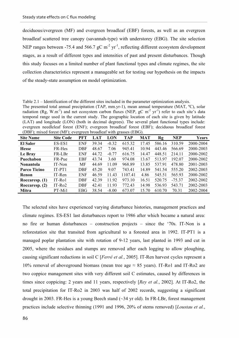
Steady state effects on C flux modeling
86
deciduous/evergreen (MF) and evergreen broadleaf (EBF) forests, as well as an evergreen
broadleaf scattered tree canopy (savannah-type) with understorey (EBG). The site selection
NEP ranges between -75.4 and 566.7 gC m-2 yr-1, reflecting different ecosystem development
stages, as a result of different types and intensities of past and present disturbances. Though
this study focuses on a limited number of plant functional types and climate regimes, the site
collection characteristics represent a manageable set for testing our hypothesis on the impacts
of the steady-state assumption on model optimization.
Table 2.1 – Identification of the different sites included in the parameter optimization analysis. The presented total annual precipitation (TAP, mm.yr-1), mean annual temperature (MAT, ºC), solar radiation (Rg, W.m-2) and net ecosystem carbon fluxes (NEP, gC m-2 yr-1) refer to each site’s data temporal range used in the current study. The geographic location of each site is given by latitude (LAT) and longitude (LON) (both in decimal degrees). The several plant functional types include: evergreen needleleaf forest (ENF); evergreen broadleaf forest (EBF); deciduous broadleaf forest (DBF); mixed forest (MF); evergreen broadleaf with grasses (EBG).
Site Name Site Code PFT LAT LON TAP MAT Rg NEP YearsEl Saler ES-ES1 ENF 39.34 -0.32 615.32 17.45 586.16 310.59 2000-2004Hesse FR-Hes DBF 48.67 7.06 945.41 10.94 443.46 566.69 2000-2003Le Bray FR-LBr ENF 44.72 -0.77 616.75 14.47 448.51 214.11 2000-2002Puechabon FR-Pue EBF 43.74 3.60 974.08 13.67 513.97 192.07 2000-2002Nonantola IT-Non MF 44.69 11.09 968.89 13.85 537.91 478.80 2001-2003Parco Ticino IT-PT1 DBF 45.20 9.07 743.41 14.89 541.54 555.20 2002-2003Renon IT-Ren ENF 46.59 11.43 1107.41 4.86 545.51 565.93 2000-2002Roccaresp. (1) IT-Ro1 DBF 42.39 11.92 973.10 16.51 520.75 -75.37 2002-2002Roccaresp. (2) IT-Ro2 DBF 42.41 11.93 772.43 14.98 536.93 543.71 2002-2003Mitra PT-Mi1 EBG 38.54 -8.00 673.07 15.70 610.70 70.31 2002-2004
The selected sites have experienced varying disturbance histories, management practices and
climate regimes. ES-ES1 last disturbances report to 1986 after which became a natural area:
no fire or human disturbances – construction projects – since the ‘70s. IT-Non is a
reforestation site that transited from agricultural to a forested area in 1992. IT-PT1 is a
managed poplar plantation site with rotation of 9-12 years, last planted in 1993 and cut in
2005, where the residues and stumps are removed after each logging to allow ploughing,
causing significant reductions in soil C [Ferré et al., 2005]. IT-Ren harvest cycles represent a
10% removal of aboveground biomass (mean tree age ≈ 85 years). IT-Ro1 and IT-Ro2 are
two coppice management sites with very different soil C estimates, caused by differences in
times since coppicing: 2 years and 11 years, respectively [Rey et al., 2002]. At IT-Ro2, the
total precipitation for IT-Ro2 in 2003 was half of 2002 records, suggesting a significant
drought in 2003. FR-Hes is a young Beech stand (~34 yr old). In FR-LBr, forest management
practices include selective thinning (1991 and 1996, 20% of stems removed) [Loustau et al.,
Materials and Methods
87
1999]. Two major disturbances were observed at this site: a wind storm in December 1999
(destroying 19.4% of the stems) and a summer drought in 2002, significantly reducing NEP.
The latest disturbances recorded in FR-Pue consist on a clear cut circa 60 years ago [Joffre et
al., 1996]. PT-Mi1 consists of a Q. suber and Q. ilex stand (≈ 90 years) strongly influenced by
drought regimes [Jarvis et al., 2007; Pereira et al., 2007].
These datasets were processed using a standardized methodology. The fluxes of CO2 were
first corrected for within-canopy CO2 storage , then controlled for insufficient turbulence (u*
filtered) and outliers (‘spikes’), and partitioned into gross primary productivity and ecosystem
respiration [Papale et al., 2006; Reichstein et al., 2005]. Uncertainties of the data processing
are discussed and quantified therein. Gap-filling was performed according to the marginal
distribution sampling method [Reichstein et al., 2005], for which uncertainties were quantified
in gap-filling in Moffat et al. [2007]. Systematic errors in eddy-covariance fluxes due to
nonideal observation conditions (e.g., advection and the imbalance in the energy budget) are
under intensive research and remain to be further quantified [Aubinet et al., 2005].
Fluxes were aggregated into daily, weekly and monthly integrals by summing up the half-
hourly gap-filled flux estimates. Flux integrals were only used for the analysis when more
than 80% of the half-hourly data were either original or gap-filled with high confidence
(Category A in Reichstein et al. [2005], also http://gaia.agraria.unitus.it/database/eddyproc/).
This is a heuristic compromise between avoiding the use of gap-filled data for model
parameterization and disregarding valuable data information.
2.3.2. Model description
The Carnegie-Ames Stanford Approach (CASA) model [Field et al., 1995; Friedlingstein et
al., 1999; Potter et al., 1993; Randerson et al., 1996] is a production efficiency model [Ruimy
et al., 1999], estimating net ecosystem production (NEP) as the difference between net
primary production (NPP) and soil heterotrophic respiration (RH). Model’s NPP estimates are
based on the concept of radiation use efficiency [Monteith, 1972; 1977] and calculated as the
product between absorbed photosynthetically active radiation (APAR) and light use efficiency
(ε):
APARNPP (2.1)
Where APAR is expressed by the product between fraction of photosynthetically active
radiation absorbed by vegetation (fAPAR) and the amount of photosynthetically active
radiation (PAR):
Steady state effects on C flux modeling
88
PARfAPARAPAR (2.2)
And ε is calculated by down-regulating maximum light use efficiency (ε*) via the effect of
temperature (Tε) and water (Wε) stress factors:
WT * (2.3)
On the other hand, RH, resulting from microbial mediated decomposition of plant and soil
organic residues, can be generically described as:
p
issiiH MTWkCR )1(
(2.4)
Where: (i) p is the number of pools; (ii) Ci is the carbon content of pool i; (iii) ki is the
maximum decay rate constant of pool i; (iv) Ws is the effect of soil moisture content on
decomposition; (v) Ts is the effect of temperature on decomposition; (vi) Mε is the carbon
assimilation efficiency of microbes. The carbon content of each pool results from the
integrated carbon transfers between litter, microbial and soil pools. In plant pools carbon is
gained through NPP and lost due to foliage, wood and root mortality and transferred to
microbial and soil organic pools. The CASA model has been widely used in studies ranging
from ecosystem to global scales [e.g. Potter et al., 2001; Randerson et al., 1996; Randerson et
al., 2002]; focusing on different ecological and biogeochemical processes [e.g. Potter et al.,
1998; Potter et al., 2001; Randerson et al., 2005]; evaluating disturbances impacts [e.g.
Masek and Collatz, 2006; van der Werf et al., 2003]; and integrated with ocean models for
global productivity studies [e.g. Behrenfeld et al., 2001; Field et al., 1998].
The CASA model is only a partial mechanistic representation of the main processes governing
carbon fluxes between the ecosystem and atmosphere. The level of complexity represents the
trade-off between biogeochemical detail and tractability for global scale studies integrating
extensive satellite observations and meteorological drivers. The parameterizations of
temperature and water stress scalars in CASA aim to reproduce mechanistic effects of both
factors on productivity and heterotrophic respiration [Field et al., 1995]. Carbon cycling
processes are based on the mechanistic compartment structure of the CENTURY model
[Parton et al., 1987] with multiple pools, each with its own turnover time, and is expected to
reproduce plausible dynamics allowing examination of the steady-state assumption on NEP
estimates. Accordingly, CASA is considered suitable to evaluate the steady-state impacts on
model performance and parameter optimization in inverse biogeochemical modelling and data
fusion exercises.
Materials and Methods
89
The CASA model inputs include climatologic drivers (mean daily, weekly, biweekly and
monthly temperature, total precipitation and solar radiation), vegetation state (plant functional
type and fractional tree cover) and biophysical properties (fAPAR and leaf area index), as well
as soil properties (texture and rooting depth).
2.3.3. Remote sensing data
In the initial CASA model implementation, seasonal vegetation biophysical properties,
fAPAR and leaf area index (LAI), were estimated through satellite remotely sensed
normalized difference vegetation index (NDVI) estimates [Potter et al., 1993]. The
emergence of robust methods for fAPAR and LAI estimations based on radiative transfer
principles [Gobron et al., 1997; Knyazikhin et al., 1998; Myneni et al., 1995] are providing
remote sensing products of significant usefulness in biophysical modelling. The current study
makes use of eight day composites of fAPAR and LAI products from the Moderate Resolution
Imaging Spectroradiometer (MODIS), on board the Terra platform [Myneni et al., 2002],
available from ORNL-DAAC [2006b]. The identification of poor quality records flagged by
ancillary datasets and the occurrence of not flagged sudden underestimation spikes (mainly
associated to atmospheric contamination) lead to the fAPAR and LAI time series treatment
based on two different methods: (i) the best index slope extraction (BISE) [Viovy et al., 1992];
and (ii) a Fourier Wave Adjustment (FWA) [Sellers et al., 1996]; both supported by robust
relationships with other variables and/or information contained from good quality
neighbouring pixels (Annex I). The rationale behind this approach is the minimization of poor
model performance in the optimization procedure resulting from low data quality issues in
input data.
2.3.4. Optimized parameters description
The first step in selecting parameter sets for optimization was the identification of scalars
governing both NPP and RH processes. Chosen parameters are mainly related to temperature
and water response curves, although maximum energy mass conversion rates (light use
efficiency) and soil carbon turn over rates were also evaluated (Table 2.2). Furthermore, a
parameter (η) was defined that scaled soil carbon pools (microbial and slow turnover rate’s
pools) at the end of the initialization process, allowing for the impact assessment of the
CCSSA in the model performance and parameter constraints. In this context, the simulation of
carbon source or sink ecosystems becomes possible by relaxing the CCSSA approach at the
end of the model spin-up, reducing the possibility of compensating effects biasing other
model parameters (Annex II).
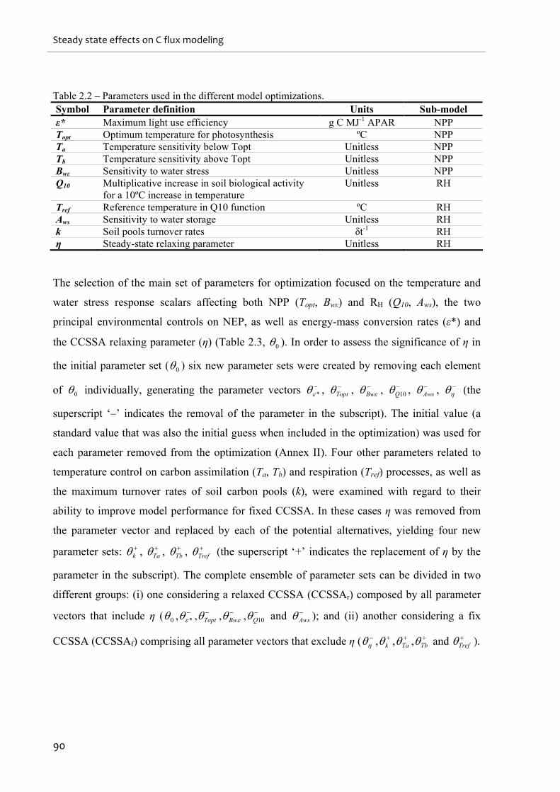
Steady state effects on C flux modeling
90
Table 2.2 – Parameters used in the different model optimizations. Symbol Parameter definition Units Sub-model ε* Maximum light use efficiency g C MJ-1 APAR NPP Topt Optimum temperature for photosynthesis ºC NPP Ta Temperature sensitivity below Topt Unitless NPP Tb Temperature sensitivity above Topt Unitless NPP Bwε Sensitivity to water stress Unitless NPP Q10 Multiplicative increase in soil biological activity
for a 10ºC increase in temperature Unitless RH
Tref Reference temperature in Q10 function ºC RH Aws Sensitivity to water storage Unitless RH k Soil pools turnover rates δt-1 RH η Steady-state relaxing parameter Unitless RH
The selection of the main set of parameters for optimization focused on the temperature and
water stress response scalars affecting both NPP (Topt, Bwε) and RH (Q10, Aws), the two
principal environmental controls on NEP, as well as energy-mass conversion rates (ε*) and
the CCSSA relaxing parameter (η) (Table 2.3, 0 ). In order to assess the significance of η in
the initial parameter set ( 0 ) six new parameter sets were created by removing each element
of 0 individually, generating the parameter vectors * ,
Topt , Bw ,
10Q , Aws ,
(the
superscript ‘–’ indicates the removal of the parameter in the subscript). The initial value (a
standard value that was also the initial guess when included in the optimization) was used for
each parameter removed from the optimization (Annex II). Four other parameters related to
temperature control on carbon assimilation (Ta, Tb) and respiration (Tref) processes, as well as
the maximum turnover rates of soil carbon pools (k), were examined with regard to their
ability to improve model performance for fixed CCSSA. In these cases η was removed from
the parameter vector and replaced by each of the potential alternatives, yielding four new
parameter sets: k ,
Ta , Tb ,
Tref (the superscript ‘+’ indicates the replacement of η by the
parameter in the subscript). The complete ensemble of parameter sets can be divided in two
different groups: (i) one considering a relaxed CCSSA (CCSSAr) composed by all parameter
vectors that include η ( 0 , * ,
Topt , Bw ,
10Q and Aws ); and (ii) another considering a fix
CCSSA (CCSSAf) comprising all parameter vectors that exclude η ( ,
k , Ta ,
Tb and Tref ).
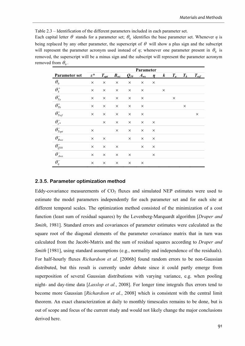
Materials and Methods
91
Table 2.3 – Identification of the different parameters included in each parameter set. Each capital letter stands for a parameter set; 0 identifies the base parameter set. Whenever η is
being replaced by any other parameter, the superscript of will show a plus sign and the subscript will represent the parameter acronym used instead of η; whenever one parameter present in 0 is
removed, the superscript will be a minus sign and the subscript will represent the parameter acronym removed from 0 .
Parameter Parameter set ε* Topt Bwε Q10 Aws η k Ta Tb Tref
0 k Ta Tb Tref *
Topt
Bw 10Q Aws
2.3.5. Parameter optimization method
Eddy-covariance measurements of CO2 fluxes and simulated NEP estimates were used to
estimate the model parameters independently for each parameter set and for each site at
different temporal scales. The optimization method consisted of the minimization of a cost
function (least sum of residual squares) by the Levenberg-Marquardt algorithm [Draper and
Smith, 1981]. Standard errors and covariances of parameter estimates were calculated as the
square root of the diagonal elements of the parameter covariance matrix that in turn was
calculated from the Jacobi-Matrix and the sum of residual squares according to Draper and
Smith [1981], using standard assumptions (e.g., normality and independence of the residuals).
For half-hourly fluxes Richardson et al. [2006b] found random errors to be non-Gaussian
distributed, but this result is currently under debate since it could partly emerge from
superposition of several Gaussian distributions with varying variance, e.g. when pooling
night- and day-time data [Lasslop et al., 2008]. For longer time integrals flux errors tend to
become more Gaussian [Richardson et al., 2008] which is consistent with the central limit
theorem. An exact characterization at daily to monthly timescales remains to be done, but is
out of scope and focus of the current study and would not likely change the major conclusions
derived here.
Steady state effects on C flux modeling
92
The parameter optimization was performed individually by site, parameter set, temporal
resolution and remote sensing correction, providing independent results in a full-factorial
design. We followed a strategy similar to Wang et al. [2006], where each optimized parameter
is normalized by its initial value, that is δ = P / P0, being P the optimized parameter and P0 the
initial parameter value. Consequently, the optimization lies on δ, rather than on P, where P
was calculated as P = δT P0, since all P0 are set the same for all simulations.
2.3.6. Statistical analysis
The CASA model performance is evaluated through different statistical indices by comparing
NEP simulations against measurements, for the different sites according to Janssen and
Heuberger [1995]. Four main indices were chosen to evaluate the model performance in
different perspectives: (i) the Normalized Average Error (NAE), expressing mean model
biases when compared to observations; (ii) the Variance Ratio (VR), aiming to analyze the
pattern of variability generated by simulations through the ratio between estimates’ and
observations’ variance; (iii) the modelling efficiency (MEF), measuring the variance of the
predictions from the one-to-one prediction line [Nash and Sutcliffe, 1970], and sensitive to
systematic deviations between model and observation [Smith et al., 1996]; as well as the
commonly used (iv) coefficient of determination, or correlation coefficient, (r2) (Annex III).
As a consequence of the current experimental design, the variance observed either in
optimized parameters or in model performance measures may be driven by different factors
(site, parameter set or temporal resolution) independently or as a result of interactions
between them. In order to identify the main determinants of variance of a given variable an n-
way analysis of variance (ANOVA) was performed for the three main factors considered, for
a 0.05 significance level [Hogg and Ledolter, 1987].
The evaluation of statistical differences between two distributions relied on one-sided
Kolmogorov-Smirnov (KS) difference tests [Janssen and Heuberger, 1995] for both higher
(F1(x) > F2(x)) and lower (F1(x) < F2(x)) alternative hypothesis. The KS tests supported the
evaluation of model performance differences between different parameter sets, as well as the
identification of differences between optimized parameters and parameters standard errors
distributions, at a significance level of 0.05, throughout sites and temporal scales.
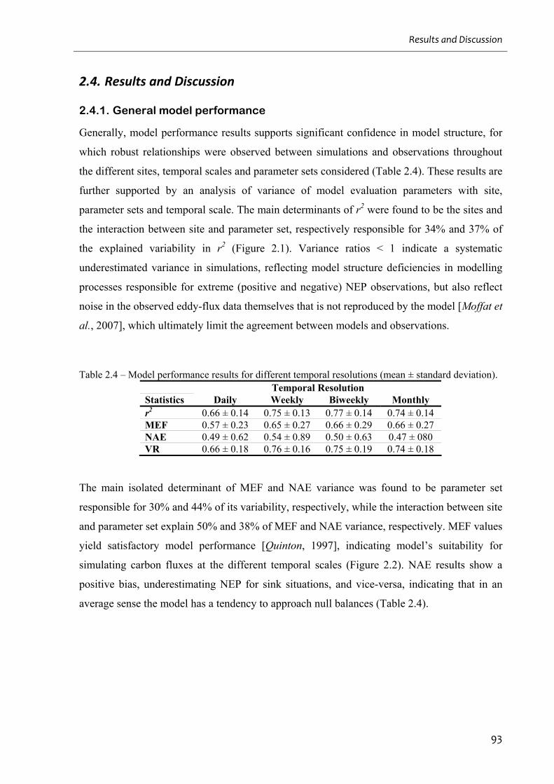
Results and Discussion
93
2.4. Results and Discussion
2.4.1. General model performance
Generally, model performance results supports significant confidence in model structure, for
which robust relationships were observed between simulations and observations throughout
the different sites, temporal scales and parameter sets considered (Table 2.4). These results are
further supported by an analysis of variance of model evaluation parameters with site,
parameter sets and temporal scale. The main determinants of r2 were found to be the sites and
the interaction between site and parameter set, respectively responsible for 34% and 37% of
the explained variability in r2 (Figure 2.1). Variance ratios < 1 indicate a systematic
underestimated variance in simulations, reflecting model structure deficiencies in modelling
processes responsible for extreme (positive and negative) NEP observations, but also reflect
noise in the observed eddy-flux data themselves that is not reproduced by the model [Moffat et
al., 2007], which ultimately limit the agreement between models and observations.
Table 2.4 – Model performance results for different temporal resolutions (mean ± standard deviation). Temporal Resolution Statistics Daily Weekly Biweekly Monthly r2 0.66 ± 0.14 0.75 ± 0.13 0.77 ± 0.14 0.74 ± 0.14 MEF 0.57 ± 0.23 0.65 ± 0.27 0.66 ± 0.29 0.66 ± 0.27 NAE 0.49 ± 0.62 0.54 ± 0.89 0.50 ± 0.63 0.47 ± 080 VR 0.66 ± 0.18 0.76 ± 0.16 0.75 ± 0.19 0.74 ± 0.18
The main isolated determinant of MEF and NAE variance was found to be parameter set
responsible for 30% and 44% of its variability, respectively, while the interaction between site
and parameter set explain 50% and 38% of MEF and NAE variance, respectively. MEF values
yield satisfactory model performance [Quinton, 1997], indicating model’s suitability for
simulating carbon fluxes at the different temporal scales (Figure 2.2). NAE results show a
positive bias, underestimating NEP for sink situations, and vice-versa, indicating that in an
average sense the model has a tendency to approach null balances (Table 2.4).
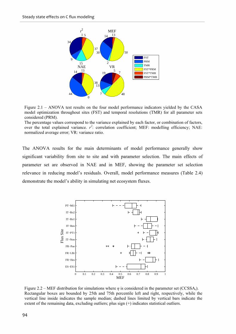
Steady state effects on C flux modeling
94
34
915
37
51r2
14
30
2
50
31MEF
14
440
38
31NAE
19
13
7 48
75
VR
FST
PRM
TMR
FST*PRM
FST*TMR
PRM*TMR
Figure 2.1 – ANOVA test results on the four model performance indicators yielded by the CASA model optimization throughout sites (FST) and temporal resolutions (TMR) for all parameter sets considered (PRM). The percentage values correspond to the variance explained by each factor, or combination of factors, over the total explained variance. r2: correlation coefficient; MEF: modelling efficiency; NAE: normalized average error; VR: variance ratio.
The ANOVA results for the main determinants of model performance generally show
significant variability from site to site and with parameter selection. The main effects of
parameter set are observed in NAE and in MEF, showing the parameter set selection
relevance in reducing model’s residuals. Overall, model performance measures (Table 2.4)
demonstrate the model’s ability in simulating net ecosystem fluxes.
0 0.1 0.2 0.3 0.4 0.5 0.6 0.7 0.8 0.9 1
ES−ES1
FR−Hes
FR−LBr
FR−Pue
IT−Non
IT−PT1
IT−Ren
IT−Ro1
IT−Ro2
PT−Mi1
MEF
Flux
Site
Figure 2.2 – MEF distribution for simulations where η is considered in the parameter set (CCSSAr). Rectangular boxes are bounded by 25th and 75th percentile left and right, respectively, while the vertical line inside indicates the sample median; dashed lines limited by vertical bars indicate the extent of the remaining data, excluding outliers; plus sign (+) indicates statistical outliers.
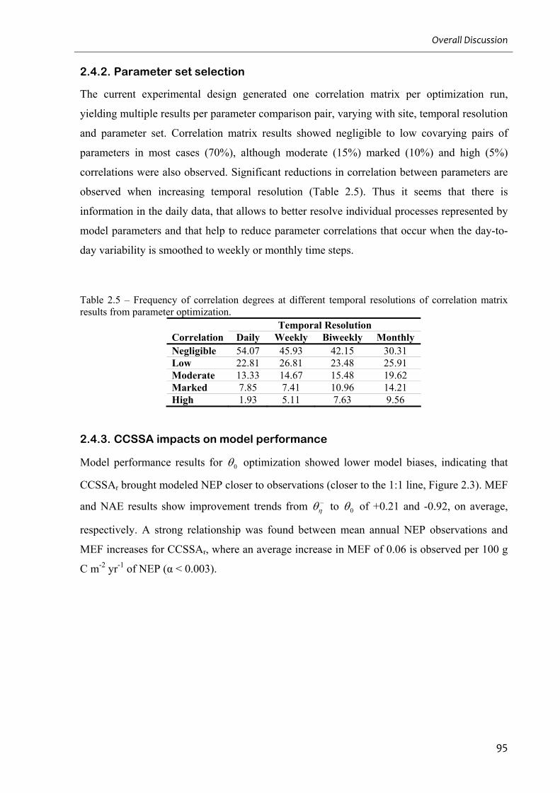
Overall Discussion
95
2.4.2. Parameter set selection
The current experimental design generated one correlation matrix per optimization run,
yielding multiple results per parameter comparison pair, varying with site, temporal resolution
and parameter set. Correlation matrix results showed negligible to low covarying pairs of
parameters in most cases (70%), although moderate (15%) marked (10%) and high (5%)
correlations were also observed. Significant reductions in correlation between parameters are
observed when increasing temporal resolution (Table 2.5). Thus it seems that there is
information in the daily data, that allows to better resolve individual processes represented by
model parameters and that help to reduce parameter correlations that occur when the day-to-
day variability is smoothed to weekly or monthly time steps.
Table 2.5 – Frequency of correlation degrees at different temporal resolutions of correlation matrix results from parameter optimization.
Temporal Resolution Correlation Daily Weekly Biweekly Monthly Negligible 54.07 45.93 42.15 30.31 Low 22.81 26.81 23.48 25.91 Moderate 13.33 14.67 15.48 19.62 Marked 7.85 7.41 10.96 14.21 High 1.93 5.11 7.63 9.56
2.4.3. CCSSA impacts on model performance
Model performance results for 0 optimization showed lower model biases, indicating that
CCSSAr brought modeled NEP closer to observations (closer to the 1:1 line, Figure 2.3). MEF
and NAE results show improvement trends from to 0 of +0.21 and -0.92, on average,
respectively. A strong relationship was found between mean annual NEP observations and
MEF increases for CCSSAr, where an average increase in MEF of 0.06 is observed per 100 g
C m-2 yr-1 of NEP (α < 0.003).
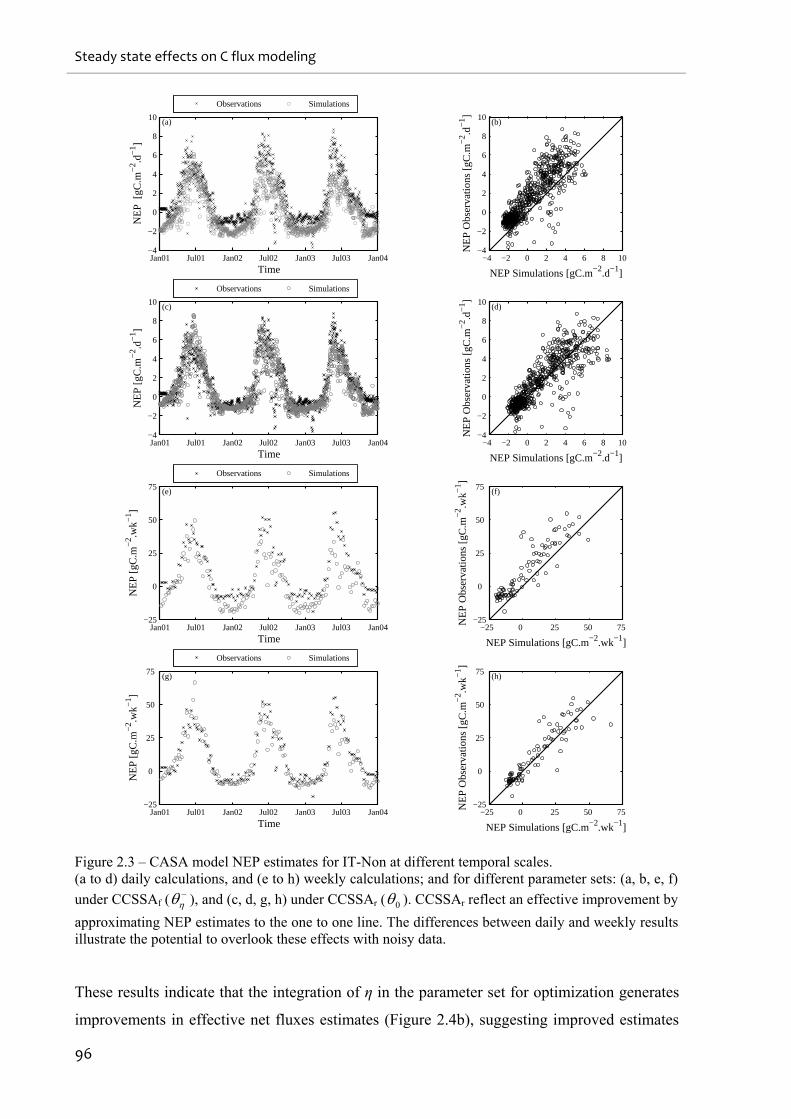
Steady state effects on C flux modeling
96
Jan01 Jul01 Jan02 Jul02 Jan03 Jul03 Jan04−4
−2
0
2
4
6
8
10
Time
NE
P [
gC.m
−2 .d
−1 ]
(a)
Observations Simulations
Jan01 Jul01 Jan02 Jul02 Jan03 Jul03 Jan04−4
−2
0
2
4
6
8
10
Time
NE
P [g
C.m
−2 .d
−1 ]
(c)
Observations Simulations
Jan01 Jul01 Jan02 Jul02 Jan03 Jul03 Jan04−25
0
25
50
75
Time
NE
P [g
C.m
−2 .w
k−1 ]
(e)
Observations Simulations
Jan01 Jul01 Jan02 Jul02 Jan03 Jul03 Jan04−25
0
25
50
75
Time
NE
P [g
C.m
−2 .w
k−1 ]
(g)
Observations Simulations
−4 −2 0 2 4 6 8 10−4
−2
0
2
4
6
8
10
NEP Simulations [gC.m−2.d−1]
NE
P O
bser
vatio
ns [
gC.m
−2 .d
−1 ]
(b)
−4 −2 0 2 4 6 8 10−4
−2
0
2
4
6
8
10
NEP Simulations [gC.m−2.d−1]N
EP
Obs
erva
tions
[gC
.m−
2 .d−
1 ]
(d)
−25 0 25 50 75 −25
0
25
50
75
NEP Simulations [gC.m−2.wk−1]
NE
P O
bser
vatio
ns [
gC.m
−2 .w
k−1 ]
(f)
−25 0 25 50 75 −25
0
25
50
75
NEP Simulations [gC.m−2.wk−1]
NE
P O
bser
vatio
ns [
gC.m
−2 .w
k−1 ]
(h)
Figure 2.3 – CASA model NEP estimates for IT-Non at different temporal scales. (a to d) daily calculations, and (e to h) weekly calculations; and for different parameter sets: (a, b, e, f)
under CCSSAf ( ), and (c, d, g, h) under CCSSAr ( 0 ). CCSSAr reflect an effective improvement by
approximating NEP estimates to the one to one line. The differences between daily and weekly results illustrate the potential to overlook these effects with noisy data.
These results indicate that the integration of η in the parameter set for optimization generates
improvements in effective net fluxes estimates (Figure 2.4b), suggesting improved estimates
Overall Discussion
97
of the other parameters and thus a better representation of environmental variability effects on
NEP. By relaxing the common steady-state assumption and hence allowing flexibility to soil
carbon pool sizes, η allows for regulation of carbon efflux from the soil as a function of
distance to an equilibrium stage, permitting higher process sensitivity to environmental
conditions. The only systematic exception to the previously referred improvements by
including η in the parameter set for optimization was PT-Mi1, which is a weak carbon sink,
generally yielding η values close to unity.
−2.5 0 2.5 5 7.5 10
(c)
θ−ε*
θ0
−2.5 0 2.5 5 7.5
NEP Simulations [gC.m−2.d−1]
(b)
θ−η
θ0
−5 −2.5 0 2.5 5 7.5−5
−2.5
0
2.5
5
7.5
10
NE
P O
bser
vatio
ns [
gC.m
−2 .d
−1 ]
(a)
θ+k
θ0
Figure 2.4 – Observations versus simulations results between different parameter sets and 0 (IT-
PT1).
Simulations without η ( ) or integrating turnover rates instead of η (
k ) in the optimization
parameter set show higher mismatch with observations (a and b). The removal of ε* ( * ) from the
initial parameter set ( 0 ) significantly affects the agreement between measured and modeled
ecosystem fluxes (c).
We further tested if the improving effect of η could also have been achieved instead by
optimizing other parameters. Replacing η with optimized soil pools maximum turn over rates
( k ) or temperature effects on NPP (
Ta and Tb ) or RH (
Tref ) produced poorer agreement
with observations than 0 optimizations. Both MEF and NAE statistics showed reductions
throughout sites and temporal scales compared to simulations where η was included to relax
the steady-state assumption (Figure 2.5). The differences between 0 versus CCSSAf
( k ,
Ta , Tb and
Tref ), evaluated independently per parameter set, show a mean increase of
0.20 to 0.36 in MEF and a mean decrease of 0.85 to 0.96 in NAE under CCSSAr conditions.
MEF differences reveal a significant relationship (α < 0.001) with mean annual NEP values
throughout temporal scales, showing an average increase in MEF of 0.04 per 100 g C m-2 yr-1
of NEP, which is consistent with the previous relationship found for 0 versus . These
results indicate that neither environment response curve related parameters ( Ta ,
Tb and
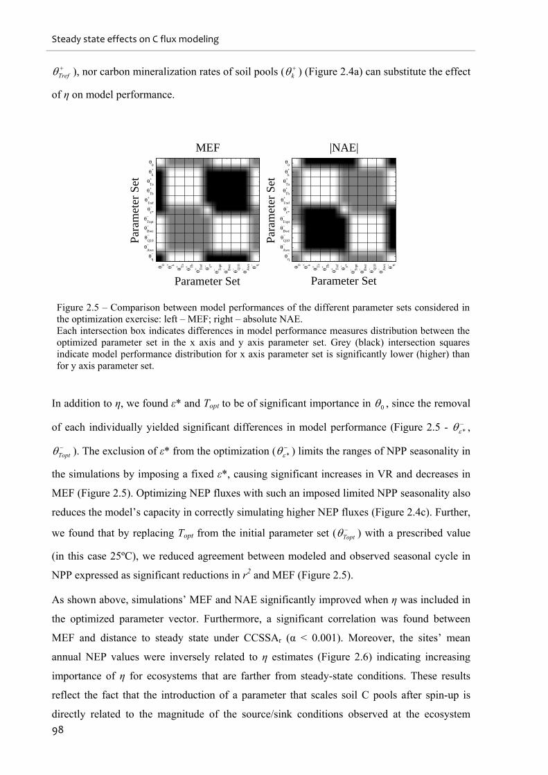
Steady state effects on C flux modeling
98
Tref ), nor carbon mineralization rates of soil pools (
k ) (Figure 2.4a) can substitute the effect
of η on model performance.
MEF
Parameter Set
Para
met
er S
et
θ 0 θ k+
θ Ta
+ θ Tb
+
θ Tre
f
+ θ ε*−
θ Top
t
− θ Bw
ε− θ Q
10
− θ Aw
s
− θ η−
θ0
θk
+
θTa
+
θTb
+
θTref
+
θε*
−
θTopt
−
θBwε−
θQ10
−
θAws
−
θη−
|NAE|
Parameter SetPa
ram
eter
Set
θ 0 θ k+
θ Ta
+ θ Tb
+
θ Tre
f
+ θ ε*−
θ Top
t
− θ Bw
ε− θ Q
10
− θ Aw
s
− θ η−
θ0
θk
+
θTa
+
θTb
+
θTref
+
θε*
−
θTopt
−
θBwε−
θQ10
−
θAws
−
θη−
Figure 2.5 – Comparison between model performances of the different parameter sets considered in the optimization exercise: left – MEF; right – absolute NAE. Each intersection box indicates differences in model performance measures distribution between the optimized parameter set in the x axis and y axis parameter set. Grey (black) intersection squares indicate model performance distribution for x axis parameter set is significantly lower (higher) than for y axis parameter set.
In addition to η, we found ε* and Topt to be of significant importance in 0 , since the removal
of each individually yielded significant differences in model performance (Figure 2.5 - * ,
Topt ). The exclusion of ε* from the optimization (
* ) limits the ranges of NPP seasonality in
the simulations by imposing a fixed ε*, causing significant increases in VR and decreases in
MEF (Figure 2.5). Optimizing NEP fluxes with such an imposed limited NPP seasonality also
reduces the model’s capacity in correctly simulating higher NEP fluxes (Figure 2.4c). Further,
we found that by replacing Topt from the initial parameter set ( Topt ) with a prescribed value
(in this case 25ºC), we reduced agreement between modeled and observed seasonal cycle in
NPP expressed as significant reductions in r2 and MEF (Figure 2.5).
As shown above, simulations’ MEF and NAE significantly improved when η was included in
the optimized parameter vector. Furthermore, a significant correlation was found between
MEF and distance to steady state under CCSSAr (α < 0.001). Moreover, the sites’ mean
annual NEP values were inversely related to η estimates (Figure 2.6) indicating increasing
importance of η for ecosystems that are farther from steady-state conditions. These results
reflect the fact that the introduction of a parameter that scales soil C pools after spin-up is
directly related to the magnitude of the source/sink conditions observed at the ecosystem
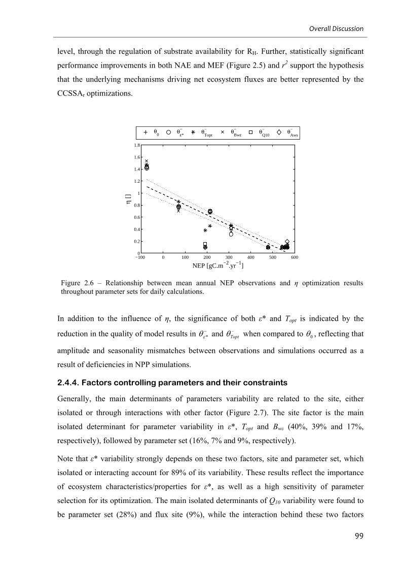
Overall Discussion
99
level, through the regulation of substrate availability for RH. Further, statistically significant
performance improvements in both NAE and MEF (Figure 2.5) and r2 support the hypothesis
that the underlying mechanisms driving net ecosystem fluxes are better represented by the
CCSSAr optimizations.
−100 0 100 200 300 400 500 6000
0.2
0.4
0.6
0.8
1
1.2
1.4
1.6
1.8
NEP [gC.m−2.yr−1]
η []
θ0
θε*− θ
Topt− θ
Bwε− θ
Q10− θ
Aws−
Figure 2.6 – Relationship between mean annual NEP observations and η optimization results throughout parameter sets for daily calculations.
In addition to the influence of η, the significance of both ε* and Topt is indicated by the
reduction in the quality of model results in * and
Topt when compared to 0 , reflecting that
amplitude and seasonality mismatches between observations and simulations occurred as a
result of deficiencies in NPP simulations.
2.4.4. Factors controlling parameters and their constraints
Generally, the main determinants of parameters variability are related to the site, either
isolated or through interactions with other factor (Figure 2.7). The site factor is the main
isolated determinant for parameter variability in ε*, Topt and Bwε (40%, 39% and 17%,
respectively), followed by parameter set (16%, 7% and 9%, respectively).
Note that ε* variability strongly depends on these two factors, site and parameter set, which
isolated or interacting account for 89% of its variability. These results reflect the importance
of ecosystem characteristics/properties for ε*, as well as a high sensitivity of parameter
selection for its optimization. The main isolated determinants of Q10 variability were found to
be parameter set (28%) and flux site (9%), while the interaction behind these two factors
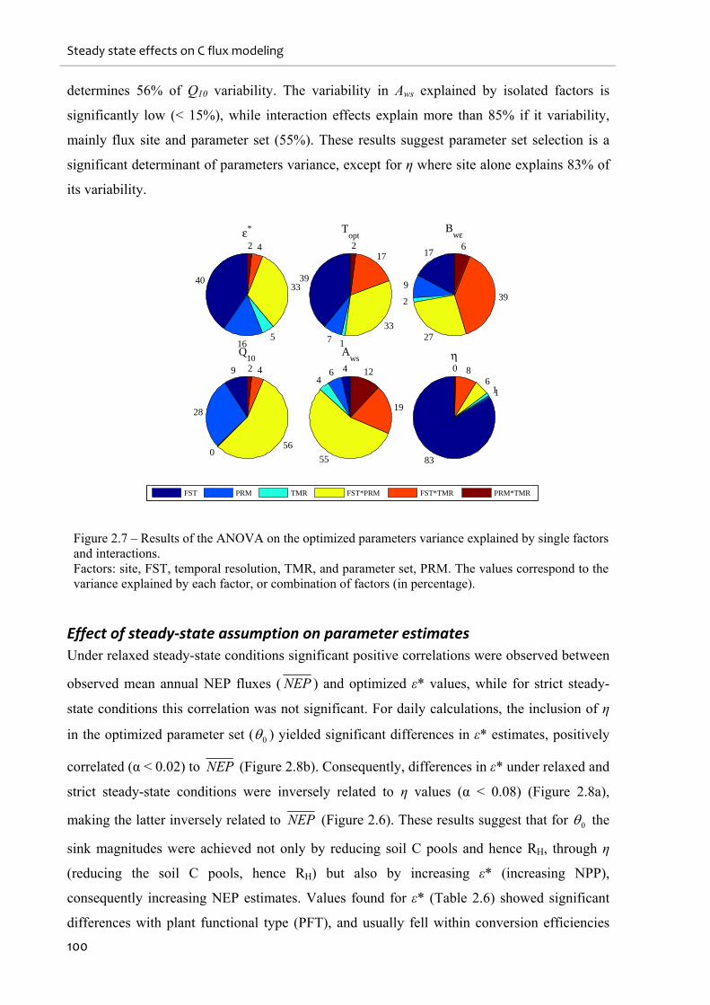
Steady state effects on C flux modeling
100
determines 56% of Q10 variability. The variability in Aws explained by isolated factors is
significantly low (< 15%), while interaction effects explain more than 85% if it variability,
mainly flux site and parameter set (55%). These results suggest parameter set selection is a
significant determinant of parameters variance, except for η where site alone explains 83% of
its variability.
40
165
33
42ε*
39
7 1
33
172
Topt
17
9
2
27
39
6
Bwε
9
28
056
42
Q10
464
55
19
12
Aws
83
116
80η
FST PRM TMR FST*PRM FST*TMR PRM*TMR
Figure 2.7 – Results of the ANOVA on the optimized parameters variance explained by single factors and interactions. Factors: site, FST, temporal resolution, TMR, and parameter set, PRM. The values correspond to the variance explained by each factor, or combination of factors (in percentage).
Effect of steady‐state assumption on parameter estimates
Under relaxed steady-state conditions significant positive correlations were observed between
observed mean annual NEP fluxes ( NEP ) and optimized ε* values, while for strict steady-
state conditions this correlation was not significant. For daily calculations, the inclusion of η
in the optimized parameter set ( 0 ) yielded significant differences in ε* estimates, positively
correlated (α < 0.02) to NEP (Figure 2.8b). Consequently, differences in ε* under relaxed and
strict steady-state conditions were inversely related to η values (α < 0.08) (Figure 2.8a),
making the latter inversely related to NEP (Figure 2.6). These results suggest that for 0 the
sink magnitudes were achieved not only by reducing soil C pools and hence RH, through η
(reducing the soil C pools, hence RH) but also by increasing ε* (increasing NPP),
consequently increasing NEP estimates. Values found for ε* (Table 2.6) showed significant
differences with plant functional type (PFT), and usually fell within conversion efficiencies
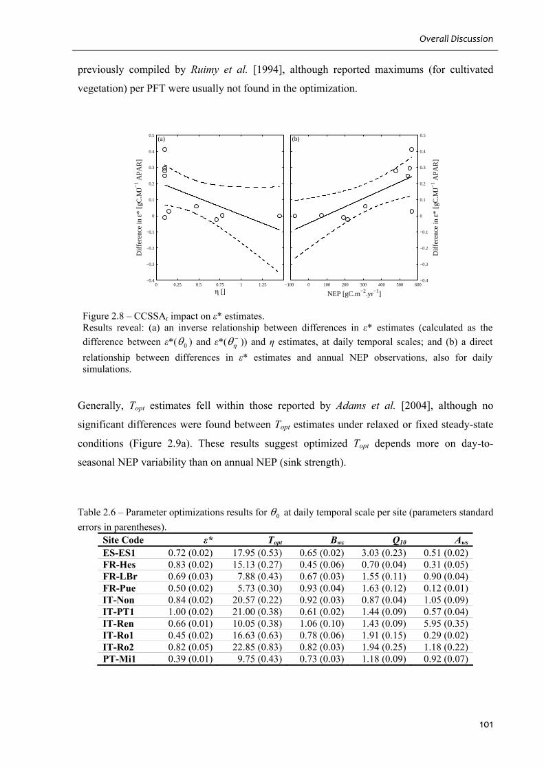
Overall Discussion
101
previously compiled by Ruimy et al. [1994], although reported maximums (for cultivated
vegetation) per PFT were usually not found in the optimization.
0 0.25 0.5 0.75 1 1.25−0.4
−0.3
−0.2
−0.1
0
0.1
0.2
0.3
0.4
0.5
η []
Dif
fere
nce
in ε*
[gC
.MJ−
1 APA
R]
(a)
−100 0 100 200 300 400 500 600−0.4
−0.3
−0.2
−0.1
0
0.1
0.2
0.3
0.4
0.5
NEP [gC.m−2.yr−1]
Dif
fere
nce
in ε*
[gC
.MJ−
1 APA
R]
(b)
Figure 2.8 – CCSSAr impact on ε* estimates. Results reveal: (a) an inverse relationship between differences in ε* estimates (calculated as the
difference between ε*( 0 ) and ε*( )) and η estimates, at daily temporal scales; and (b) a direct
relationship between differences in ε* estimates and annual NEP observations, also for daily simulations.
Generally, Topt estimates fell within those reported by Adams et al. [2004], although no
significant differences were found between Topt estimates under relaxed or fixed steady-state
conditions (Figure 2.9a). These results suggest optimized Topt depends more on day-to-
seasonal NEP variability than on annual NEP (sink strength).
Table 2.6 – Parameter optimizations results for 0 at daily temporal scale per site (parameters standard
errors in parentheses). Site Code ε* Topt Bwε Q10 Aws
ES-ES1 0.72 (0.02) 17.95 (0.53) 0.65 (0.02) 3.03 (0.23) 0.51 (0.02)FR-Hes 0.83 (0.02) 15.13 (0.27) 0.45 (0.06) 0.70 (0.04) 0.31 (0.05)FR-LBr 0.69 (0.03) 7.88 (0.43) 0.67 (0.03) 1.55 (0.11) 0.90 (0.04)FR-Pue 0.50 (0.02) 5.73 (0.30) 0.93 (0.04) 1.63 (0.12) 0.12 (0.01)IT-Non 0.84 (0.02) 20.57 (0.22) 0.92 (0.03) 0.87 (0.04) 1.05 (0.09)IT-PT1 1.00 (0.02) 21.00 (0.38) 0.61 (0.02) 1.44 (0.09) 0.57 (0.04)IT-Ren 0.66 (0.01) 10.05 (0.38) 1.06 (0.10) 1.43 (0.09) 5.95 (0.35)IT-Ro1 0.45 (0.02) 16.63 (0.63) 0.78 (0.06) 1.91 (0.15) 0.29 (0.02)IT-Ro2 0.82 (0.05) 22.85 (0.83) 0.82 (0.03) 1.94 (0.25) 1.18 (0.22)PT-Mi1 0.39 (0.01) 9.75 (0.43) 0.73 (0.03) 1.18 (0.09) 0.92 (0.07)
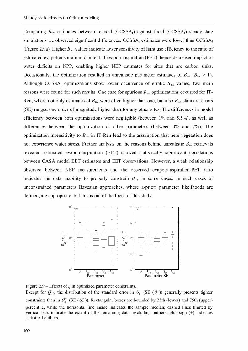
Steady state effects on C flux modeling
102
Comparing Bwε estimates between relaxed (CCSSAr) against fixed (CCSSAf) steady-state
simulations we observed significant differences: CCSSAr estimates were lower than CCSSAf
(Figure 2.9a). Higher Bwε values indicate lower sensitivity of light use efficiency to the ratio of
estimated evapotranspiration to potential evapotranspiration (PET), hence decreased impact of
water deficits on NPP, enabling higher NEP estimates for sites that are carbon sinks.
Occasionally, the optimization resulted in unrealistic parameter estimates of Bwε (Bwε > 1).
Although CCSSAr optimizations show lower occurrence of erratic Bwε values, two main
reasons were found for such results. One case for spurious Bwε optimizations occurred for IT-
Ren, where not only estimates of Bwε were often higher than one, but also Bwε standard errors
(SE) ranged one order of magnitude higher than for any other sites. The differences in model
efficiency between both optimizations were negligible (between 1% and 5.5%), as well as
differences between the optimization of other parameters (between 0% and 7%). The
optimization insensitivity to Bwε in IT-Ren lead to the assumption that here vegetation does
not experience water stress. Further analysis on the reasons behind unrealistic Bwε retrievals
revealed estimated evapotranspiration (EET) showed statistically significant correlations
between CASA model EET estimates and EET observations. However, a weak relationship
observed between NEP measurements and the observed evapotranspiration-PET ratio
indicates the data inability to properly constrain Bwε in some cases. In such cases of
unconstrained parameters Bayesian approaches, where a-priori parameter likelihoods are
defined, are appropriate, but this is out of the focus of this study.
10−1
100
101
θ 0 / θ η−
[]
Parameterε* T
optB
wε Q10
Aws
(a)
10−2
10−1
100
101
102
θ 0 / θ η−
[]
Parameter SEε* T
optB
wε Q10
Aws
(b)
Figure 2.9 – Effects of η in optimized parameter constraints. Except for Q10, the distribution of the standard error in 0 (SE ( 0 )) generally presents tighter
constraints than in (SE (
)). Rectangular boxes are bounded by 25th (lower) and 75th (upper)
percentile, while the horizontal line inside indicates the sample median; dashed lines limited by vertical bars indicate the extent of the remaining data, excluding outliers; plus sign (+) indicates statistical outliers.
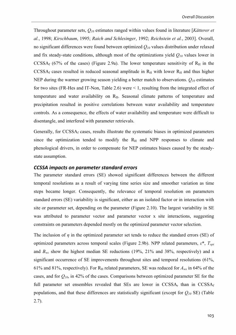
Overall Discussion
103
Throughout parameter sets, Q10 estimates ranged within values found in literature [Kätterer et
al., 1998; Kirschbaum, 1995; Raich and Schlesinger, 1992; Reichstein et al., 2003]. Overall,
no significant differences were found between optimized Q10 values distribution under relaxed
and fix steady-state conditions, although most of the optimizations yield Q10 values lower in
CCSSAf (67% of the cases) (Figure 2.9a). The lower temperature sensitivity of RH in the
CCSSAf cases resulted in reduced seasonal amplitude in RH with lower RH and thus higher
NEP during the warmer growing season yielding a better match to observations. Q10 estimates
for two sites (FR-Hes and IT-Non, Table 2.6) were < 1, resulting from the integrated effect of
temperature and water availability on RH. Seasonal climate patterns of temperature and
precipitation resulted in positive correlations between water availability and temperature
controls. As a consequence, the effects of water availability and temperature were difficult to
disentangle, and interfered with parameter retrievals.
Generally, for CCSSAf cases, results illustrate the systematic biases in optimized parameters
since the optimization tended to modify the RH and NPP responses to climate and
phenological drivers, in order to compensate for NEP estimates biases caused by the steady-
state assumption.
CCSSA impacts on parameter standard errors
The parameter standard errors (SE) showed significant differences between the different
temporal resolutions as a result of varying time series size and smoother variation as time
steps became longer. Consequently, the relevance of temporal resolution on parameters
standard errors (SE) variability is significant, either as an isolated factor or in interaction with
site or parameter set, depending on the parameter (Figure 2.10). The largest variability in SE
was attributed to parameter vector and parameter vector x site interactions, suggesting
constraints on parameters depended mostly on the optimized parameter vector selection.
The inclusion of η in the optimized parameter set tends to reduce the standard errors (SE) of
optimized parameters across temporal scales (Figure 2.9b). NPP related parameters, ε*, Topt
and Bwε show the highest median SE reductions (19%, 21% and 38%, respectively) and a
significant occurrence of SE improvements throughout sites and temporal resolutions (61%,
61% and 81%, respectively). For RH related parameters, SE was reduced for Aws in 64% of the
cases, and for Q10, in 42% of the cases. Comparisons between optimized parameter SE for the
full parameter set ensembles revealed that SEs are lower in CCSSAr than in CCSSAf
populations, and that these differences are statistically significant (except for Q10 SE) (Table
2.7).
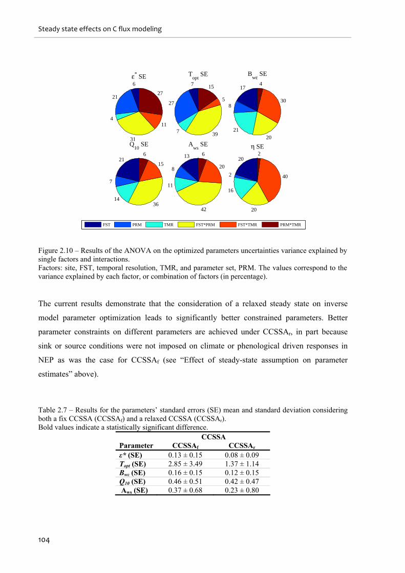
Steady state effects on C flux modeling
104
6
21
4
31
11
27
ε* SE7
27
7 39
5
15
Topt
SE
17
8
2120
30
4
Bwε
SE
21
7
1436
15
6
Q10
SE
13
8
11
42
20
6
Aws
SE
20
2
16
20
40
2η SE
FST PRM TMR FST*PRM FST*TMR PRM*TMR
Figure 2.10 – Results of the ANOVA on the optimized parameters uncertainties variance explained by single factors and interactions. Factors: site, FST, temporal resolution, TMR, and parameter set, PRM. The values correspond to the variance explained by each factor, or combination of factors (in percentage).
The current results demonstrate that the consideration of a relaxed steady state on inverse
model parameter optimization leads to significantly better constrained parameters. Better
parameter constraints on different parameters are achieved under CCSSAr, in part because
sink or source conditions were not imposed on climate or phenological driven responses in
NEP as was the case for CCSSAf (see “Effect of steady-state assumption on parameter
estimates” above).
Table 2.7 – Results for the parameters’ standard errors (SE) mean and standard deviation considering both a fix CCSSA (CCSSAf) and a relaxed CCSSA (CCSSAr). Bold values indicate a statistically significant difference.
CCSSA Parameter CCSSAf CCSSAr ε* (SE) 0.13 ± 0.15 0.08 ± 0.09 Topt (SE) 2.85 ± 3.49 1.37 ± 1.14 Bwε (SE) 0.16 ± 0.15 0.12 ± 0.15 Q10 (SE) 0.46 ± 0.51 0.42 ± 0.47 Aws (SE) 0.37 ± 0.68 0.23 ± 0.80
Overall Discussion
105
2.4.5. Relaxation of the carbon cycle steady state
As shown above, the variability in η was strongly determined by inter site variability and
much less so by temporal resolution or parameter set, corroborating the previous correlation
between η and magnitude of the source or sink behaviour of each site (Figure 2.6). The
CCSSAr approach forced the adjustments of C pools after spin-up routines, regulating each
site’s respiration potential hence modifying the differences between mean annual NPP and RH
fluxes. These results suggest ecosystem respiration (RECO) controls on net ecosystem carbon
exchange [Valentini et al., 2000]. The parameter η and measured ECORNEP (considered a
normalized distance measure from equilibrium) were significantly correlated (α < 0.05) for all
relaxed steady-state parameters sets. Yet, significant positive correlations found between
NEP (and also ECORNEP ) and ε* in relaxed steady-state optimizations suggest stronger
sinks are associated with marked NPP seasonality. These results imply a significant role of
mean annual gross primary productivity (GPP ) in determining net ecosystem carbon
exchange (Figure 2.11).
Figure 2.11 – Mean annual net ecosystem production (NEP) versus mean annual gross primary production (GPP, r2 = 0.96, α < 0.0001) and ecosystem respiration (RECO, r2 = 0.002, α < 0.91), estimated from flux partitioning.
In summary, we find that in the CCSSAr approach allows for the simulation of C sinks, by
decreasing the soil C pools, hence the RH potential. However, the observed correlations
between GPP and NEP (and GPP and ε*) suggest that sink magnitudes not only depend on
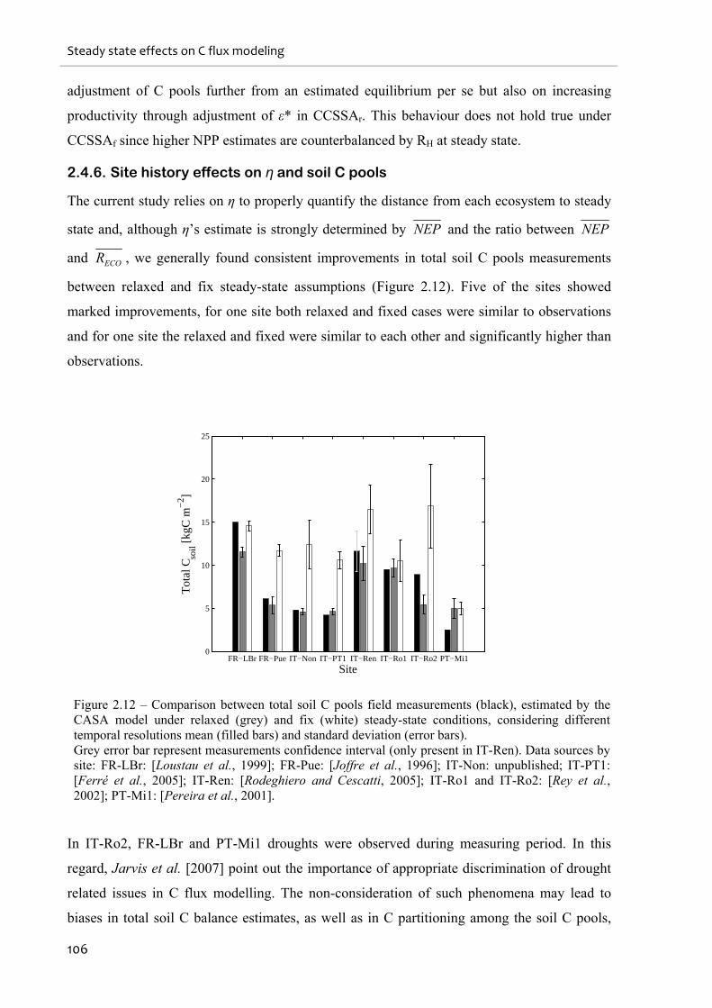
Steady state effects on C flux modeling
106
adjustment of C pools further from an estimated equilibrium per se but also on increasing
productivity through adjustment of ε* in CCSSAr. This behaviour does not hold true under
CCSSAf since higher NPP estimates are counterbalanced by RH at steady state.
2.4.6. Site history effects on η and soil C pools
The current study relies on η to properly quantify the distance from each ecosystem to steady
state and, although η’s estimate is strongly determined by NEP and the ratio between NEP
and ECOR , we generally found consistent improvements in total soil C pools measurements
between relaxed and fix steady-state assumptions (Figure 2.12). Five of the sites showed
marked improvements, for one site both relaxed and fixed cases were similar to observations
and for one site the relaxed and fixed were similar to each other and significantly higher than
observations.
FR−LBr FR−Pue IT−Non IT−PT1 IT−Ren IT−Ro1 IT−Ro2 PT−Mi10
5
10
15
20
25
Tot
al C
soil [
kgC
m−
2 ]
Site
Figure 2.12 – Comparison between total soil C pools field measurements (black), estimated by the CASA model under relaxed (grey) and fix (white) steady-state conditions, considering different temporal resolutions mean (filled bars) and standard deviation (error bars). Grey error bar represent measurements confidence interval (only present in IT-Ren). Data sources by site: FR-LBr: [Loustau et al., 1999]; FR-Pue: [Joffre et al., 1996]; IT-Non: unpublished; IT-PT1: [Ferré et al., 2005]; IT-Ren: [Rodeghiero and Cescatti, 2005]; IT-Ro1 and IT-Ro2: [Rey et al., 2002]; PT-Mi1: [Pereira et al., 2001].
In IT-Ro2, FR-LBr and PT-Mi1 droughts were observed during measuring period. In this
regard, Jarvis et al. [2007] point out the importance of appropriate discrimination of drought
related issues in C flux modelling. The non-consideration of such phenomena may lead to
biases in total soil C balance estimates, as well as in C partitioning among the soil C pools,
Overall Discussion
107
which is of significant importance in regions prone to systematic droughts, as is the case of
PT-Mi1 [Pereira et al., 2001; Pereira et al., 2007]. Furthermore, in these areas, spin-up
routines may also yield significant biases in soil C pools by prescribing transient climate
datasets based on averages or smoothed time series, where climate variability and extremes
are removed or reduced.
Although the current results demonstrate that relaxed steady-state assumptions through η
approximate modeled from measured total soil C pools, some important assumptions were
made regarding soil C pools, disturbances and inter-annual variability (IAV): i) although total
soil C pools estimates improved in CCSSAr optimizations, a correct partitioning between the
different soil C pools is not assumed, due to η’s undifferentiated nature; ii) being η strongly
related to NEP , and the ECORNEP ratio, the relationship between η and disturbances is only
possible if these cause variations in annual C balance; and iii) when uniquely analyzing
individual years, IAV can be a source of error in the quantification of the distance to steady
state.
2.4.7. Potential applications of the CCSSAr in biogeochemical modelling
The concept of capturing the disequilibrium in carbon fluxes through a parameter η has
potential implications and applications for generalizing carbon fluxes from site to regional
scales. Following the two-component modelling approach by Andrén and Kätterer [1997],
first order soil C dynamics equations can be analytically solved for both pools at steady state
(Annex IV). Assuming non steady-state conditions, η can be calculated as:
GPPf
NEP
h
11 ,
(2.5)
where h stands for the “humification coefficient”, expressing the fraction of annual C fluxes
entering a carbon pool with long turnover times, and GPPf describes the mean annual input
of C to the soil, which in steady state is assumed equivalent to observations of mean annual
NPP ( NPP ), considered a constant fraction of GPP [Waring et al., 1998]. Our results show
significant correlations (α < 0.002) between η and GPPNEP with an offset of 1.026 ± 0.027
and a slope of -3.043 ± 0.088, implying an h of 0.7 ± 0.02, considering an f of 0.47 [Waring et
al., 1998]. Estimates found for h are significantly above values reported by Andrén and
Kätterer [1997] (ranging from 0.13 to 0.34), possibly reflecting a carbon sequestration in
multiple pools including woody material, while Andrén and Kätterer [1997] considered
herbaceous ecosystems [Kätterer et al., 1998].
Steady state effects on C flux modeling
108
These results suggest an approach to integrate top-down and bottom-up approaches in C flux
modelling, as exemplified in Rayner et al. [2005]. The main goal would be to quantify
spatially the distance to steady-state conditions in terrestrial ecosystems by constraining the
soil C pools with NEP estimates from atmospheric inversions, and GPP (or NPP ) estimates
from the ecosystem biogeochemical model. Using equation 5 one could give an estimate of η
that could be compared to disturbance and land-use history.
2.5. Overall Discussion
The current model evaluation study quantifies the ability of the CASA model to simulate
carbon fluxes at the ecosystem scale, and indicates a significant robustness in estimating NEP
of ten eddy-covariance monitoring sites at different temporal scales. CASA is well suited to
evaluate the impact of the steady-state approach on model performance and parameterization
through one parameter, η, which relaxes this assumption. The consideration of a relaxed
versus a strict steady-state approach produces: (i) significant increases in model performance,
via increases in MEF and reductions in NAE; and (ii) improvements in parameter constraints.
The correlation between η and differences in model performance emphasizes the positive
impact of a CCSSAr the farther apart an ecosystem is from equilibrium. Overall, a clear
distinction can be made between CCSSAr and CCSSAf model performance results although a
significant inter-site variability is observed both in model performance as well as in the results
of the parameter optimization. Changes in the optimization results of environmental response
parameters associated with significant increases in model performance under CCSSAr suggest
parameterization biases under fixed steady-state assumption, mainly on NPP related
parameters.
The relevance of optimizing ε* is emphasized in this selection of sites, where GPP is driving
NEP observations, and not ECOR , as commonly found [Reichstein et al., 2007]. The current
study demonstrates modeled sink/source magnitudes can be improved by considering both a
parameter η quantifying the distance to an estimated steady-state situation, yielding
adjustments in total C pools closer to measurements; and adjustments to primary production
through ε* Furthermore, the significance of synchronizing NEP seasonal cycles through Topt is
emphasized by significant improvements in model performance. Potential biases in η can
occur due to strong NEP inter-annual variability, suggesting the consideration of time series
of multiple years for a robust analysis of η.
Overall Discussion
109
As a limitation we note however, that these calculations hinge on the accuracy of annual sums
of eddy-covariance flux data, which might even after state-of-the-art corrections
underestimate night-time fluxes and hence overestimate NEP. There are clear indications that
errors are site dependent and need further investigation [e.g. Aubinet et al., 2005; Belelli-
Marchesini et al., 2007; Marcolla et al., 2005].
From a more generalized modelling perspective the current study demonstrates the usefulness
of model-data synthesis approaches for testing conceptual principles used in biogeochemical
modelling. In this sense the importance of appropriate and flexible model structures is
emphasized, since we showed that inappropriate structure in one part of the model can
introduce biased parameter estimates in apparently unrelated other model parts via statistical
correlations.
2.6. Conclusions
While previous studies have shown the potential of model inversion against eddy-covariance
data and have emphasized the importance of data error characterization, our study shows the
implications of a typical biogeochemical model structure on model performance and
parameter retrieval for the first time in a systematic way. Furthermore, our results emphasize
the need for future studies on model structure, both in the context of diagnostic as well as
prognostic models.
While the overall ability of the CASA model to simulate ecosystem carbon fluxes has been
confirmed here, the limitations of the carbon cycle steady-state assumption (CCSSA)
embodied in almost all biogeochemical modelling approaches has been clearly disclosed. We
show that the CCSSA deteriorates not only model performance expressed as model errors or
modelling efficiency, but more importantly, leads to biased parameter retrieval in a model-
data fusion framework. Indicative of this, the relaxation of the CCSSA via one parameter η
that relates to imbalance of soil carbon pools yielded better model performance and more
constrained parameter estimates. Hence our study clearly demonstrates that implications of
model structure for inverse parameter retrieval deserve more attention. In particular the
common steady-state assumption may compromise model-data synthesis in biogeochemical
modelling and needs to be addressed thoroughly. In our study we used a semi-empirical
correction approach, but future solutions might include a more explicit simulation of reasons
for non-steady state in parameter optimization procedures.
Results and Discussion
110
Acknowledgements
We are grateful to Chris Neigh and Martin Jung for helpful comments on the manuscript and
for always fruitful discussions. We are also thankful to James Randerson, David Hollinger and
one anonymous reviewer for constructive comments that very much helped improving the
manuscript. This work was funded by the Portuguese Foundation for Science and Technology
(FCT) under the CARBERIAN project (contract no. PDCTE/CTA/49985/2003). NC
acknowledges the support given by the Portuguese Foundation for Science and Technology
(FCT), the European Union under Operational Program “Science and Innovation” (POCI
2010), PhD grant ref. SFRH/BD/6517/2001, co-sponsored by the European Social Fund, and
the Marie-Curie Reintegration Grant GLUES (MC MERG-CT-2005-031077) to MR.
Research leading to flux data and scientific insight was supported by the CARBOEUROPE-IP
project.
References
Adams, B., A. White, and T. M. Lenton (2004), An analysis of some diverse approaches to modelling terrestrial net primary productivity, Ecol Model, 177(3-4), 353-391.
Amthor, J. S., J. M. Chen, J. S. Clein, S. E. Frolking, M. L. Goulden, R. F. Grant, J. S. Kimball, A. W. King, A. D. McGuire, N. T. Nikolov, C. S. Potter, S. Wang, and S. C. Wofsy (2001), Boreal forest CO2 exchange and evapotranspiration predicted by nine ecosystem process models: Intermodel comparisons and relationships to field measurements, J Geophys Res-Atmos, 106(D24), 33623-33648.
Andrén, O., and T. Kätterer (1997), ICBM: The introductory carbon balance model for exploration of soil carbon balances, Ecol Appl, 7(4), 1226-1236.
Aubinet, M., A. Grelle, A. Ibrom, U. Rannik, J. Moncrieff, T. Foken, A. S. Kowalski, P. H. Martin, P. Berbigier, C. Bernhofer, R. Clement, J. Elbers, A. Granier, T. Grunwald, K. Morgenstern, K. Pilegaard, C. Rebmann, W. Snijders, R. Valentini, and T. Vesala (2000), Estimates of the annual net carbon and water exchange of forests: The EUROFLUX methodology, Advances in Ecological Research, 30, 113-175.
Aubinet, M., P. Berbigier, C. Bernhofer, A. Cescatti, C. Feigenwinter, A. Granier, T. Grunwald, K. Havrankova, B. Heinesch, B. Longdoz, B. Marcolla, L. Montagnani, and P. Sedlak (2005), Comparing CO2 storage and advection conditions at night at different carboeuroflux sites, Bound-Lay Meteorol, 116(1), 63-94.
Baldocchi, D., J. Finnigan, K. Wilson, K. T. Paw U, and E. Falge (2000), On measuring net ecosystem carbon exchange over tall vegetation on complex terrain, Bound-Lay Meteorol, 96(1-2), 257-291.
Barrett, D. J. (2002), Steady state turnover time of carbon in the Australian terrestrial biosphere, Global Biogeochem Cy, 16(4).
Behrenfeld, M. J., J. T. Randerson, C. R. McClain, G. C. Feldman, S. O. Los, C. J. Tucker, P. G. Falkowski, C. B. Field, R. Frouin, W. E. Esaias, D. D. Kolber, and N. H. Pollack (2001), Biospheric primary production during an ENSO transition, Science, 291(5513), 2594-2597.
References
111
Belelli-Marchesini, L., D. Papale, M. Reichstein, N. Vuichard, N. Tchebakova, and R. Valentini (2007), Carbon balance assessment of a natural steppe of southern Siberia by multiple constraint approach, Biogeosciences, 4(4), 581-595.
Box, E. O. (1988), Estimating the Seasonal Carbon Source-Sink Geography of a Natural, Steady-State Terrestrial Biosphere, J Appl Meteorol, 27(10), 1109-1124.
Cannell, M. G. R., and J. H. M. Thornley (2003), Ecosystem productivity is independent of some soil properties at equilibrium, Plant Soil, 257(1), 193-204.
Draper, N., and H. Smith (1981), Applied Regression Analysis, Wiley, New York.
Dufrêne, E., H. Davi, C. Francois, G. le Maire, V. Le Dantec, and A. Granier (2005), Modelling carbon and water cycles in a beech forest Part I: Model description and uncertainty analysis on modelled NEE, Ecol Model, 185(2-4), 407-436.
Epron, D., V. Le Dantec, E. Dufrêne, and A. Granier (2001), Seasonal dynamics of soil carbon dioxide efflux and simulated rhizosphere respiration in a beech forest, Tree Physiol, 21(2-3), 145-152.
Falge, E., D. Baldocchi, J. Tenhunen, M. Aubinet, P. Bakwin, P. Berbigier, C. Bernhofer, G. Burba, R. Clement, K. J. Davis, J. A. Elbers, A. H. Goldstein, A. Grelle, A. Granier, J. Guomundsson, D. Hollinger, A. S. Kowalski, G. Katul, B. E. Law, Y. Malhi, T. Meyers, R. K. Monson, J. W. Munger, W. Oechel, K. T. Paw, K. Pilegaard, U. Rannik, C. Rebmann, A. Suyker, R. Valentini, K. Wilson, and S. Wofsy (2002), Seasonality of ecosystem respiration and gross primary production as derived from FLUXNET measurements, Agr Forest Meteorol, 113(1-4), 53-74.
Ferré, C., A. Leip, G. Matteucci, F. Previtali, and G. Seufert (2005), Impact of 40 years poplar cultivation on soil carbon stocks and greenhouse gas fluxes, Biogeosciences Discuss., 2(4), 897-931.
Field, C. B., J. T. Randerson, and C. M. Malmstrom (1995), Global Net Primary Production - Combining Ecology and Remote-Sensing, Remote Sens Environ, 51(1), 74-88.
Field, C. B., M. J. Behrenfeld, J. T. Randerson, and P. Falkowski (1998), Primary production of the biosphere: Integrating terrestrial and oceanic components, Science, 281(5374), 237-240.
Friedlingstein, P., G. Joel, C. B. Field, and I. Y. Fung (1999), Toward an allocation scheme for global terrestrial carbon models, Global Change Biol, 5(7), 755-770.
Gobron, N., B. Pinty, M. M. Verstraete, and Y. Govaerts (1997), A semidiscrete model for the scattering of light by vegetation, J Geophys Res-Atmos, 102(D8), 9431-9446.
Hogg, R. V., and J. Ledolter (1987), Engineering Statistics, Macmillan, New York.
Janssen, P. H. M., and P. S. C. Heuberger (1995), Calibration of Process-Oriented Models, Ecol Model, 83(1-2), 55-66.
Jarvis, P., A. Rey, C. Petsikos, L. Wingate, M. Rayment, J. Pereira, J. Banza, J. David, F. Miglietta, M. Borghetti, G. Manca, and R. Valentini (2007), Drying and wetting of Mediterranean soils stimulates decomposition and carbon dioxide emission: the "Birch effect", Tree Physiol, 27(7), 929-940.
Joffre, R., S. Rambal, and F. Romane (1996), Local variations of ecosystem functions in Mediterranean evergreen oak woodland, Ann Sci Forest, 53(2-3), 561-570.
Kätterer, T., M. Reichstein, O. Andren, and A. Lomander (1998), Temperature dependence of organic matter decomposition: a critical review using literature data analyzed with different models, Biol Fert Soils, 27(3), 258-262.
Steady state effects on C flux modeling
112
Kirschbaum, M. U. F. (1995), The Temperature-Dependence of Soil Organic-Matter Decomposition, and the Effect of Global Warming on Soil Organic-C Storage, Soil Biol Biochem, 27(6), 753-760.
Knyazikhin, Y., J. V. Martonchik, R. B. Myneni, D. J. Diner, and S. W. Running (1998), Synergistic algorithm for estimating vegetation canopy leaf area index and fraction of absorbed photosynthetically active radiation from MODIS and MISR data, J Geophys Res-Atmos, 103(D24), 32257-32275.
Lasslop, G., M. Reichstein, J. Kattge, and D. Papale (2008), Influences of observation errors in eddy flux data on inverse model parameter estimation, Biogeosciences, 5(5), 1311-1324.
Law, B. E., R. H. Waring, P. M. Anthoni, and J. D. Aber (2000), Measurements of gross and net ecosystem productivity and water vapour exchange of a Pinus ponderosa ecosystem, and an evaluation of two generalized models, Global Change Biol, 6(2), 155-168.
Law, B. E., F. M. Kelliher, D. D. Baldocchi, P. M. Anthoni, J. Irvine, D. Moore, and S. Van Tuyl (2001), Spatial and temporal variation in respiration in a young ponderosa pine forests during a summer drought, Agr Forest Meteorol, 110(1), 27-43.
Loustau, D., P. Berbigier, A. Granier, Y. Brunet, T. Bariac, and R. Valentini (1999), Measuring the carbon balance of European forests: Case studies of the two French sites from the Euroflux Network: Short-term environmental controls on carbon dioxide flux in a boreal coniferous forest: Model computation compared with measurements by eddy, Comptes-rendus des Seances de l'Academie d'Agriculture de France, 85(6), 255–264.
Lugo, A. E., and S. Brown (1986), Steady-State Terrestrial Ecosystems and the Global Carbon-Cycle, Vegetatio, 68(2), 83-90.
Marcolla, B., A. Cescatti, L. Montagnani, G. Manca, G. Kerschbaumer, and S. Minerbi (2005), Importance of advection in the atmospheric CO2 exchanges of an alpine forest, Agr Forest Meteorol, 130(3-4), 193-206.
Masek, J. G., and G. J. Collatz (2006), Estimating forest carbon fluxes in a disturbed southeastern landscape: Integration of remote sensing, forest inventory, and biogeochemical modeling, J Geophys Res-Biogeo, 111(G1).
Moffat, A. M., D. Papale, M. Reichstein, D. Y. Hollinger, A. D. Richardson, A. G. Barr, C. Beckstein, B. H. Braswell, G. Churkina, A. R. Desai, E. Falge, J. H. Gove, M. Heimann, D. Hui, A. J. Jarvis, J. Kattge, A. Noormets, and V. J. Stauch (2007), Comprehensive comparison of gap-filling techniques for eddy covariance net carbon fluxes, Agr Forest Meteorol, 147(3-4), 209-232.
Monteith, J. L. (1972), Solar-Radiation and Productivity in Tropical Ecosystems, J Appl Ecol, 9(3), 747-766.
Monteith, J. L. (1977), Climate and Efficiency of Crop Production in Britain, Philos T Roy Soc B, 281(980), 277-294.
Morales, P., M. T. Sykes, I. C. Prentice, P. Smith, B. Smith, H. Bugmann, B. Zierl, P. Friedlingstein, N. Viovy, S. Sabate, A. Sanchez, E. Pla, C. A. Gracia, S. Sitch, A. Arneth, and J. Ogee (2005), Comparing and evaluating process-based ecosystem model predictions of carbon and water fluxes in major European forest biomes, Global Change Biol, 11(12), 2211-2233.
Myneni, R. B., S. Maggion, J. Iaquinto, J. L. Privette, N. Gobron, B. Pinty, D. S. Kimes, M. M. Verstraete, and D. L. Williams (1995), Optical Remote-Sensing of Vegetation - Modeling, Caveats, and Algorithms, Remote Sens Environ, 51(1), 169-188.
References
113
Myneni, R. B., S. Hoffman, Y. Knyazikhin, J. L. Privette, J. Glassy, Y. Tian, Y. Wang, X. Song, Y. Zhang, G. R. Smith, A. Lotsch, M. Friedl, J. T. Morisette, P. Votava, R. R. Nemani, and S. W. Running (2002), Global products of vegetation leaf area and fraction absorbed PAR from year one of MODIS data, Remote Sens Environ, 83(1-2), 214-231.
Nash, J. E., and J. V. Sutcliffe (1970), River flow forecasting through conceptual models part I -- A discussion of principles, Journal of Hydrology, 10(3), 282-290.
ORNL-DAAC (2006a), FLUXNET Integrating Worldwide CO2 Flux Measurements, edited, ORNL DAAC, Oak Ridge, Tennessee, U.S.A.
ORNL-DAAC (2006b), MODIS subsetted land products, Collection 4, edited, ORNL DAAC, Oak Ridge, Tennessee, U.S.A.
Papale, D., and A. Valentini (2003), A new assessment of European forests carbon exchanges by eddy fluxes and artificial neural network spatialization, Global Change Biol, 9(4), 525-535.
Papale, D., M. Reichstein, M. Aubinet, E. Canfora, C. Bernhofer, W. Kutsch, B. Longdoz, S. Rambal, R. Valentini, T. Vesala, and D. Yakir (2006), Towards a standardized processing of Net Ecosystem Exchange measured with eddy covariance technique: algorithms and uncertainty estimation, Biogeosciences, 3, 571-583.
Parton, W. J., D. S. Schimel, C. V. Cole, and D. S. Ojima (1987), Analysis of Factors Controlling Soil Organic-Matter Levels in Great-Plains Grasslands, Soil Sci Soc Am J, 51(5), 1173-1179.
Pereira, J. S., M. Chaves, J. S. David, T. S. David, M. Rayment, M. Vaz, and J. Banza (2001), The importance of drought in the control of water and carbon fluxes in an evergreen oak woodland in southwest Iberian Peninsula, Ecol. Soc. Am. Annu. Meet. Abstr., 86,176.
Pereira, J. S., J. A. Mateus, L. M. Aires, G. Pita, C. Pio, J. S. David, V. Andrade, J. Banza, T. S. David, T. A. Paco, and A. Rodrigues (2007), Net ecosystem carbon exchange in three contrasting Mediterranean ecosystems - the effect of drought, Biogeosciences, 4(5), 791-802.
Pietsch, S. A., and H. Hasenauer (2006), Evaluating the self-initialization procedure for large-scale ecosystem models, Global Change Biol, 12(9), 1658-1669.
Potter, C. S., J. T. Randerson, C. B. Field, P. A. Matson, P. M. Vitousek, H. A. Mooney, and S. A. Klooster (1993), Terrestrial Ecosystem Production - a Process Model-Based on Global Satellite and Surface Data, Global Biogeochem Cy, 7(4), 811-841.
Potter, C. S., E. A. Davidson, S. A. Klooster, D. C. Nepstad, G. H. De Negreiros, and V. Brooks (1998), Regional application of an ecosystem production model for studies of biogeochemistry in Brazilian Amazonia, Global Change Biol, 4(3), 315-333.
Potter, C. S., S. E. Alexander, J. C. Coughlan, and S. A. Klooster (2001), Modeling biogenic emissions of isoprene: exploration of model drivers, climate control algorithms, and use of global satellite observations, Atmos Environ, 35(35), 6151-6165.
Quinton, J. N. (1997), Reducing predictive uncertainty in model simulations: a comparison of two methods using the European Soil Erosion Model (EUROSEM), Catena, 30(2-3), 101-117.
Raich, J. W., and W. H. Schlesinger (1992), The Global Carbon-Dioxide Flux in Soil Respiration and Its Relationship to Vegetation and Climate, Tellus B, 44(2), 81-99.
Randerson, J. T., M. V. Thompson, C. M. Malmstrom, C. B. Field, and I. Y. Fung (1996), Substrate limitations for heterotrophs: Implications for models that estimate the seasonal cycle of atmospheric CO2, Global Biogeochem Cy, 10(4), 585-602.
Steady state effects on C flux modeling
114
Randerson, J. T., C. J. Still, J. J. Balle, I. Y. Fung, S. C. Doney, P. P. Tans, T. J. Conway, J. W. C. White, B. Vaughn, N. Suits, and A. S. Denning (2002), Carbon isotope discrimination of arctic and boreal biomes inferred from remote atmospheric measurements and a biosphere-atmosphere model, Global Biogeochem Cy, 16(3), doi:10.1029/2001GB001435
Randerson, J. T., G. R. van der Werf, G. J. Collatz, L. Giglio, C. J. Still, P. Kasibhatla, J. B. Miller, J. W. C. White, R. S. DeFries, and E. S. Kasischke (2005), Fire emissions from C-3 and C-4 vegetation and their influence on interannual variability of atmospheric CO2 and delta(CO2)-C-13, Global Biogeochem Cy, 19(2), -, DOI: 10.1029/2004GB002366.
Rannik, U., P. Kolari, T. Vesala, and P. Hari (2006), Uncertainties in measurement and modelling of net ecosystem exchange of a forest, Agr Forest Meteorol, 138(1-4), 244-257.
Rayner, P. J., M. Scholze, W. Knorr, T. Kaminski, R. Giering, and H. Widmann (2005), Two decades of terrestrial carbon fluxes from a carbon cycle data assimilation system (CCDAS), Global Biogeochem Cy, 19(2), doi:10.1029/2004GB002254.
Reichstein, M., J. Tenhunen, O. Roupsard, J. M. Ourcival, S. Rambal, F. Miglietta, A. Peressotti, M. Pecchiari, G. Tirone, and R. Valentini (2003), Inverse modeling of seasonal drought effects on canopy CO2/H2O exchange in three Mediterranean ecosystems, J Geophys Res-Atmos, 108(D23).
Reichstein, M., E. Falge, D. Baldocchi, D. Papale, M. Aubinet, P. Berbigier, C. Bernhofer, N. Buchmann, T. Gilmanov, A. Granier, T. Grunwald, K. Havrankova, H. Ilvesniemi, D. Janous, A. Knohl, T. Laurila, A. Lohila, D. Loustau, G. Matteucci, T. Meyers, F. Miglietta, J. M. Ourcival, J. Pumpanen, S. Rambal, E. Rotenberg, M. Sanz, J. Tenhunen, G. Seufert, F. Vaccari, T. Vesala, D. Yakir, and R. Valentini (2005), On the separation of net ecosystem exchange into assimilation and ecosystem respiration: review and improved algorithm, Global Change Biol, 11(9), 1424-1439.
Reichstein, M., D. Papale, R. Valentini, M. Aubinet, C. Bernhofer, A. Knohl, T. Laurila, A. Lindroth, E. Moors, K. Pilegaard, and G. Seufert (2007), Determinants of terrestrial ecosystem carbon balance inferred from European eddy covariance flux sites, Geophys Res Lett, 34(1), doi:10.1029/2006GL027880.
Rey, A., E. Pegoraro, V. Tedeschi, I. De Parri, P. G. Jarvis, and R. Valentini (2002), Annual variation in soil respiration and its components in a coppice oak forest in Central Italy, Global Change Biol, 8(9), 851-866.
Richardson, A. D., B. H. Braswell, D. Y. Hollinger, P. Burman, E. A. Davidson, R. S. Evans, L. B. Flanagan, J. W. Munger, K. Savage, S. P. Urbanski, and S. C. Wofsy (2006a), Comparing simple respiration models for eddy flux and dynamic chamber data, Agr Forest Meteorol, 141(2-4), 219-234.
Richardson, A. D., D. Y. Hollinger, G. G. Burba, K. J. Davis, L. B. Flanagan, G. G. Katul, J. W. Munger, D. M. Ricciuto, P. C. Stoy, A. E. Suyker, S. B. Verma, and S. C. Wofsy (2006b), A multi-site analysis of random error in tower-based measurements of carbon and energy fluxes, Agr Forest Meteorol, 136(1-2), 1-18.
Richardson, A. D., M. D. Mahecha, E. Falge, J. Kattge, A. M. Moffat, D. Papale, M. Reichstein, V. J. Stauch, B. H. Braswell, G. Churkina, B. Kruijt, and D. Y. Hollinger (2008), Statistical properties of random CO2 flux measurement uncertainty inferred from model residuals, Agr Forest Meteorol, 148(1), 38-50.
Rodeghiero, M., and A. Cescatti (2005), Main determinants of forest soil respiration along an elevation/temperature gradient in the Italian Alps, Global Change Biol, 11(7), 1024-1041.
References
115
Ruimy, A., B. Saugier, and G. Dedieu (1994), Methodology for the estimation of terrestrial net primary productivity production from remotely sensed data, Journal of Geophysical Research, 99(D20), 5263-5283.
Ruimy, A., L. Kergoat, A. Bondeau, and Participants Potsdam NPP Model Intercomparison (1999), Comparing global models of terrestrial net primary productivity (NPP): analysis of differences in light absorption and light-use efficiency, Global Change Biol, 5, 56-64.
Schimel, D. S., B. H. Braswell, and W. J. Parton (1997), Equilibration of the terrestrial water, nitrogen, and carbon cycles, P Natl Acad Sci USA, 94(16), 8280-8283.
Sellers, P. J., S. O. Los, C. J. Tucker, C. O. Justice, D. A. Dazlich, G. J. Collatz, and D. A. Randall (1996), A revised land surface parameterization (SiB2) for atmospheric GCMs .2. The generation of global fields of terrestrial biophysical parameters from satellite data, J Climate, 9(4), 706-737.
Smith, J. U., P. Smith, and T. M. Addiscott (1996), Quantitative methods to evaluate and compare soil organic matter (SOM) models, in Evaluation of soil organic matter models : using existing long-term datasets, edited by D. S. Powlson, et al., pp. 181 - 199, Springer-Verlag, New York.
Tenhunen, J. D., R. Valentini, B. Kostner, R. Zimmermann, and A. Granier (1998), Variation in forest gas exchange at landscape to continental scales, Ann Sci Forest, 55(1-2), 1-11.
Trudinger, C. M., M. R. Raupach, P. J. Rayner, J. Kattge, Q. Liu, B. Pak, M. Reichstein, L. Renzullo, A. D. Richardson, S. H. Roxburgh, J. Styles, Y. P. Wang, P. Briggs, D. Barrett, and S. Nikolova (2007), OptIC project: An intercomparison of optimization techniques for parameter estimation in terrestrial biogeochemical models, J Geophys Res-Biogeo, 112(G2), doi:10.1029/2006JG000367.
Valentini, R., G. Matteucci, A. J. Dolman, E. D. Schulze, C. Rebmann, E. J. Moors, A. Granier, P. Gross, N. O. Jensen, K. Pilegaard, A. Lindroth, A. Grelle, C. Bernhofer, T. Grunwald, M. Aubinet, R. Ceulemans, A. S. Kowalski, T. Vesala, U. Rannik, P. Berbigier, D. Loustau, J. Guomundsson, H. Thorgeirsson, A. Ibrom, K. Morgenstern, R. Clement, J. Moncrieff, L. Montagnani, S. Minerbi, and P. G. Jarvis (2000), Respiration as the main determinant of carbon balance in European forests, Nature, 404(6780), 861-865.
van der Werf, G. R., J. T. Randerson, G. J. Collatz, and L. Giglio (2003), Carbon emissions from fires in tropical and subtropical ecosystems, Global Change Biol, 9(4), 547-562.
Viovy, N., O. Arino, and A. S. Belward (1992), The Best Index Slope Extraction (Bise) - a Method for Reducing Noise in NDVI Time-Series, Int J Remote Sens, 13(8), 1585-1590.
Wang, Y. P., D. Baldocchi, R. A. Y. Leuning, E. V. A. Falge, and T. Vesala (2006), Estimating parameters in a land-surface model by applying nonlinear inversion to eddy covariance flux measurements from eight FLUXNET sites, Global Change Biol, 12, 1-12.
Waring, R. H., J. J. Landsberg, and M. Williams (1998), Net primary production of forests: a constant fraction of gross primary production?, Tree Physiol, 18(2), 129-134.
Wutzler, T., and M. Reichstein (2007), Soils apart from equilibrium – consequences for soil carbon balance modelling, Biogeosciences, 4(1), 125-136.
Xu, T., L. White, D. F. Hui, and Y. Q. Luo (2006), Probabilistic inversion of a terrestrial ecosystem model: Analysis of uncertainty in parameter estimation and model prediction, Global Biogeochem Cy, 20(2).

117
Chapter 3 – Identification of Vegetation and Soil Carbon Pools Out
of Equilibrium in a Process Model Via Eddy‐Covariance and
Biometric Constraints
3.1. Summary
Assumptions of steady-state conditions in biogeochemical modelling are often invoked
because knowledge on the development status of the modelling domain is generally
unavailable. Here, we investigate the role of vegetation pool sizes on nonequilibrium
conditions through model-data integration approaches for a set of sites using eddy-covariance
CO2 flux data. The study is based on the Carnegie Ames Stanford Approach (CASA) model,
modified (CASAG) in order to evaluate the sensitivity of simulated net ecosystem production
(NEP) fluxes to vegetation pool sizes. The experimental design is based on the inverse model
optimization of different parameter vectors performed at the measurement site level. Each
parameter vector prescribes different simulation dynamics that embody different model
structural assumptions concerning (non) steady-state conditions in vegetation and soil carbon
pools. We further explore the potential of assimilating biometric constraints through the cost
function for sites where in situ information on above ground biomass or wood pools is
available. The integration of biometric data yields marked improvements in the simulation of
vegetation C pools compared to single only-eddy-flux constraints. Overall, it is necessary to
relax both vegetation and soil carbon pools for consistency with the observed data streams.
Multiple constraints approaches also leads to variable model performance among the different
experimental setups and model structures. We identify and assess the limitations of various
model structures and the role of multiple constraints approaches for tackling issues of
equifinality. These studies emphasize the need for establishing consistent data sets of fluxes
and biometric data for successful model-data fusion.
3.2. Introduction
Recent advances in global carbon cycle research have emphasized the significance of
biosphere-atmosphere interactions. Understanding and quantification of carbon cycle-climate
Ecosystem C pools apart from equilibrium
118
system feedbacks are key for reducing uncertainty in prognostic modelling [e.g. Bonan, 2008;
Friedlingstein et al., 2006; Heimann and Reichstein, 2008]. Biogeochemical modelling
approaches are required to address these topics, and observational data should lay the
foundations for identifying modelling structures and constraining parameterizations [O'Neill
and Melnikov, 2008]. Model-data integration studies have contributed significantly to these
issues through inverse modelling approaches from local to global scales [e.g. Knorr and
Kattge, 2005; Lauvaux et al., 2008; Scholze et al., 2007].
In biogeochemical modelling, the lack of information on current states or past-history of the
ecosystem within the modelling domain often leads to a priori assumptions of equilibrium
states for estimating initial conditions of carbon (C) pools [Odum, 1969]. Initialization
routines consist of iterative model runs repeating climate conditions until equilibrium, or
steady state, when biosphere-atmosphere net C exchanges approach zero at the annual scale;
these can be followed by transient runs where climate transitions and management practices
are prescribed [Morales et al., 2005]. The steady-state assumption for the ecosystem carbon
cycle has been challenged [e.g. Cannell and Thornley, 2003; Lugo and Brown, 1986;
Luyssaert et al., 2008] and its limitations in modelling approaches emphasized [Pietsch and
Hasenauer, 2006; Wutzler and Reichstein, 2007].
Moreover, the implications of the steady-state assumption for inverse modelling approaches
applied to nonsteady-state ecosystems have been previously reported [Carvalhais et al.,
2008]. To reach steady state, the long term C pools are incremented until ecosystem C influx
and efflux is balanced and quasi-neutral net fluxes define the initial conditions of the model
optimization. Consequently, the optimization of parameters governing fluxes that depend on
the magnitude of C pools may lead to compensatory biases and limit the model ability to
mimic the observed fluxes. Following an empirical approach, the steady state was relaxed via
one specific parameter η that scaled the soil pools following the spin-up to equilibrium,
creating an imbalance in NEP fluxes by adjusting the soil carbon pools. This improved the
model’s ability to simulate the observations – the model performance – but also resolved
biases in estimates of parameters that control the responses of net primary production (NPP)
and heterotrophic respiration (RH) to temperature and water availability. The implications of
nonsteady-state conditions for model-data integration approaches were explicitly related to the
initial condition problem through soil C pools, although disequilibrium in live vegetation C
pools can also be a key factor [Luo et al., 2001; Santaren et al., 2007; Schaefer et al., 2008].
Vegetation C pools contribute to ecosystem carbon fluxes directly through autotrophic
Introduction
119
respiration (RA) and indirectly through C transfers to the soil and litter pools – supplying the
substrate for RH.
The accumulation of C in vegetation pools with slow turnover rates (woody pools) represents
a significant fraction of the total C in mature ecosystems. In contrast to C pools that turnover
more rapidly, woody C pools require longer periods to achieve new “equilibrium” conditions
after natural or human induced disturbances. The direct and indirect effects of management
regimes, historical land-use changes and/or natural disturbances have significant implications
on ecosystem C sink / source magnitudes at decadal time scales [Barford et al., 2001;
Nabuurs, 2004]. These perturbations impact the ecosystem C flow between vegetation, litter,
and soil pools. The prescription of such dynamics can significantly improve ecosystem
models [Thornton et al., 2002]. In this regard, the slow dynamics of woody C pools may be
expected to influence model performance and parameter estimation as has been shown for soil
C pools.
We aim to examine if ecosystem sink or source conditions could be partially or fully
explained by nonequilibrium states in slow turnover vegetation C pools (wood) and in soil C
pools. We hypothesize that errors in net ecosystem fluxes estimation induced by steady-state
conditions cannot be circumvented by solely relaxing woody pools because other pools (soil
and litter) with similar turnover rates are likely to significantly affect estimates of carbon
fluxes. The importance of wood and/or soil C pools magnitudes for NEP estimates emerges
from the model-data agreement of different model structures. We further ask whether the
assimilation of carbon fluxes from eddy-covariance and biometric measurements improves
our ability to identify limitations stemming from model structure.
Differing initial states, parameterizations or model structures can yield similar model
performance results: representing equifinality [e.g. Franks et al., 1997; Medlyn et al., 2005].
Model vulnerability to equifinality, among other factors, can be associated with the gap
between parameterized processes and observational constraints [e.g. Beven, 1989]; as well as
with limited variability in inputs and observations [e.g. Franks et al., 1997]. Thus, the
emergence of issues related to equifinality may compromise confidence in prognostic
simulations: process misrepresentation may be unimportant at short time scales albeit
significant at longer time scales [Crout et al., 2009; Fox et al., 2009]. Here we address these
issues by evaluating different model structures and integrating C flux data representative of
different temporal scales, in an attempt to identify and resolve equifinality issues.
Ecosystem C pools apart from equilibrium
120
For this study we modify the Carnegie Ames Stanford Approach (CASA) model [Potter et al.,
1993] to enable the prescription of direct and indirect effects of C wood pools on net
ecosystem production (NEP). We further implement a systematic experimental design to test
the significance of the vegetation woody C pools on nonsteady-state conditions in model
parameter optimization.
3.3. Materials and Methods
3.3.1. Eddy-covariance sites data
The current study focuses on a set of eddy-covariance sites in the Carboeurope-IP network of
eddy-covariance flux measurement towers (http://www.carboeurope.org). The sites were
selected as representative of Mediterranean climate classes or ecosystems present in the
Iberian Peninsula (Table 3.1). Further, the selected sites met minimum data availability
requirements for: 1) remotely sensed leaf area index and fraction of photosynthetically active
radiation absorbed by vegetation; and 2) in situ daily measurements of climate variables
(temperature, precipitation and solar radiation) and ecosystem C fluxes. The CO2 fluxes were
first corrected for within-canopy CO2 storage and then controlled for insufficient turbulence
(u* filtered) and outliers (‘spikes’) [Papale et al., 2006]. Daily flux integrals were only used
for the analysis when more than 80% of the half-hourly data were either original or gap-filled
with high confidence (Category A in Reichstein et al. [2005]).
The collection of selected sites (Table 3.1) represents a range of different disturbance
backgrounds, management practices and climate regimes. ES-ES1 became a natural area in
1986 and no fire events or human disturbances have been recorded since the 1970s. FR-Hes is
a young Beech stand (~34 yr old) [Granier et al., 2008]. In FR-LBr, forest management
practices include selective thinning (1991 and 1996, 20% of stems removed) [Loustau et al.,
1999]. The latest disturbances recorded in FR-Pue consist of a clear cut circa 60 years ago
[Joffre et al., 1996]. In 1992, IT-Non transited from an agricultural to a forested area. IT-PT1
is a managed poplar plantation site with rotation of 9-12 years, last planted in 1993 and
harvested in 2005; here, the residues and stumps are removed after each logging [Ferré et al.,
2005; Migliavacca et al., 2009]. IT-Ren is located on an unevenly aged coniferous forest
[Montagnani et al., 2009] with mean tree age of ~85 years and the harvest cycles represent a
10% removal of aboveground biomass. IT-Ro1 and IT-Ro2 are two coppice management sites
with very different times since coppicing: 2 years and 11 years, respectively [Rey et al., 2002].
PT-Mi1 consists of a Quercus suber L. and Quercus ilex L. stand (~90 years) strongly
influenced by drought regimes [Jarvis et al., 2007; Pereira et al., 2007].
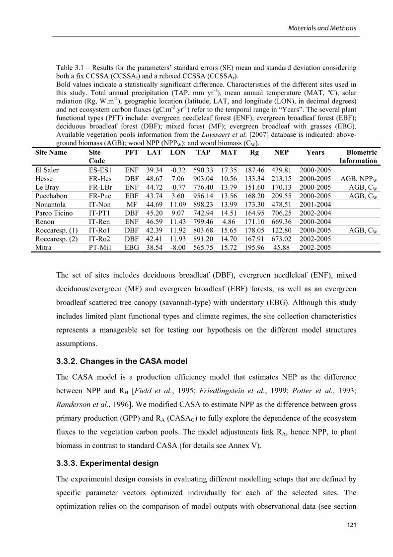
Materials and Methods
121
Table 3.1 – Results for the parameters’ standard errors (SE) mean and standard deviation considering both a fix CCSSA (CCSSAf) and a relaxed CCSSA (CCSSAr). Bold values indicate a statistically significant difference. Characteristics of the different sites used in this study. Total annual precipitation (TAP, mm yr-1), mean annual temperature (MAT, ºC), solar radiation (Rg, W.m-2), geographic location (latitude, LAT, and longitude (LON), in decimal degrees) and net ecosystem carbon fluxes (gC.m-2.yr-1) refer to the temporal range in “Years”. The several plant functional types (PFT) include: evergreen needleleaf forest (ENF); evergreen broadleaf forest (EBF); deciduous broadleaf forest (DBF); mixed forest (MF); evergreen broadleaf with grasses (EBG). Available vegetation pools information from the Luyssaert et al. [2007] database is indicated: above-ground biomass (AGB); wood NPP (NPPW); and wood biomass (CW).
Site Name Site Code
PFT LAT LON TAP MAT Rg NEP Years Biometric Information
El Saler ES-ES1 ENF 39.34 -0.32 590.33 17.35 187.46 439.81 2000-2005 Hesse FR-Hes DBF 48.67 7.06 903.04 10.56 133.34 213.15 2000-2005 AGB, NPPW
Le Bray FR-LBr ENF 44.72 -0.77 776.40 13.79 151.60 170.13 2000-2005 AGB, CW
Puechabon FR-Pue EBF 43.74 3.60 956.14 13.56 168.20 209.55 2000-2005 AGB, CW
Nonantola IT-Non MF 44.69 11.09 898.23 13.99 173.30 478.51 2001-2004 Parco Ticino IT-PT1 DBF 45.20 9.07 742.94 14.51 164.95 706.25 2002-2004 Renon IT-Ren ENF 46.59 11.43 799.46 4.86 171.10 669.36 2000-2004 Roccaresp. (1) IT-Ro1 DBF 42.39 11.92 803.68 15.65 178.05 122.80 2000-2005 AGB, CW
Roccaresp. (2) IT-Ro2 DBF 42.41 11.93 891.20 14.70 167.91 673.02 2002-2005 Mitra PT-Mi1 EBG 38.54 -8.00 565.75 15.72 195.96 45.88 2002-2005
The set of sites includes deciduous broadleaf (DBF), evergreen needleleaf (ENF), mixed
deciduous/evergreen (MF) and evergreen broadleaf (EBF) forests, as well as an evergreen
broadleaf scattered tree canopy (savannah-type) with understory (EBG). Although this study
includes limited plant functional types and climate regimes, the site collection characteristics
represents a manageable set for testing our hypothesis on the different model structures
assumptions.
3.3.2. Changes in the CASA model
The CASA model is a production efficiency model that estimates NEP as the difference
between NPP and RH [Field et al., 1995; Friedlingstein et al., 1999; Potter et al., 1993;
Randerson et al., 1996]. We modified CASA to estimate NPP as the difference between gross
primary production (GPP) and RA (CASAG) to fully explore the dependence of the ecosystem
fluxes to the vegetation carbon pools. The model adjustments link RA, hence NPP, to plant
biomass in contrast to standard CASA (for details see Annex V).
3.3.3. Experimental design
The experimental design consists in evaluating different modelling setups that are defined by
specific parameter vectors optimized individually for each of the selected sites. The
optimization relies on the comparison of model outputs with observational data (see section
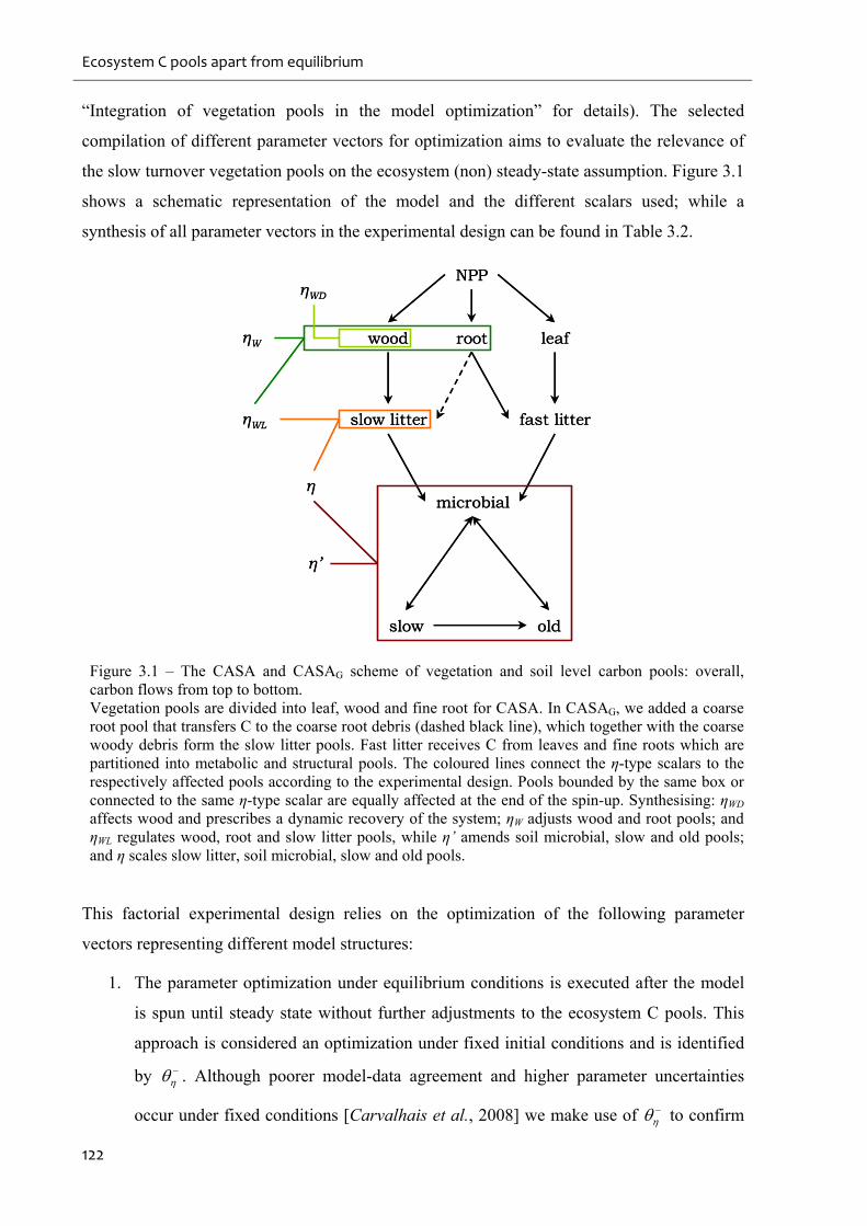
Ecosystem C pools apart from equilibrium
122
“Integration of vegetation pools in the model optimization” for details). The selected
compilation of different parameter vectors for optimization aims to evaluate the relevance of
the slow turnover vegetation pools on the ecosystem (non) steady-state assumption. Figure 3.1
shows a schematic representation of the model and the different scalars used; while a
synthesis of all parameter vectors in the experimental design can be found in Table 3.2.
fast litter
microbial
slow
slow litter
old
root leaf
NPP
ηWL
η’
η
ηWD
ηW wood
fast litter
microbial
slow
slow litter
old
root leaf
NPP
ηWL
η’
η
ηWD
ηW wood
Figure 3.1 – The CASA and CASAG scheme of vegetation and soil level carbon pools: overall, carbon flows from top to bottom. Vegetation pools are divided into leaf, wood and fine root for CASA. In CASAG, we added a coarse root pool that transfers C to the coarse root debris (dashed black line), which together with the coarse woody debris form the slow litter pools. Fast litter receives C from leaves and fine roots which are partitioned into metabolic and structural pools. The coloured lines connect the η-type scalars to the respectively affected pools according to the experimental design. Pools bounded by the same box or connected to the same η-type scalar are equally affected at the end of the spin-up. Synthesising: ηWD affects wood and prescribes a dynamic recovery of the system; ηW adjusts wood and root pools; and ηWL regulates wood, root and slow litter pools, while η’ amends soil microbial, slow and old pools; and η scales slow litter, soil microbial, slow and old pools.
This factorial experimental design relies on the optimization of the following parameter
vectors representing different model structures:
1. The parameter optimization under equilibrium conditions is executed after the model
is spun until steady state without further adjustments to the ecosystem C pools. This
approach is considered an optimization under fixed initial conditions and is identified
by . Although poorer model-data agreement and higher parameter uncertainties
occur under fixed conditions [Carvalhais et al., 2008] we make use of to confirm
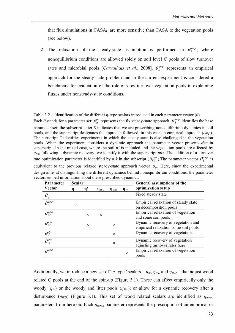
Materials and Methods
123
that flux simulations in CASAG are more sensitive than CASA to the vegetation pools
(see below).
2. The relaxation of the steady-state assumption is performed in empS , where
nonequilibrium conditions are allowed solely on soil level C pools of slow turnover
rates and microbial pools [Carvalhais et al., 2008]. empS represents an empirical
approach for the steady-state problem and in the current experiment is considered a
benchmark for evaluation of the role of slow turnover vegetation pools in explaining
fluxes under nonsteady-state conditions.
Table 3.2 – Identification of the different η-type scalars introduced in each parameter vector (θ).
Each θ stands for a parameter set; represents the fix steady-state approach. emp
S identifies the base
parameter set: the subscript letter S indicates that we are prescribing nonequilibrium dynamics in soil pools, and the superscript designates the approach followed, in this case an empirical approach (emp). The subscript V identifies experiments in which the steady state is also challenged in the vegetation pools. When the experiment considers a dynamic approach the parameter vector presents dyn in superscript. In the mixed case, where the soil η’ is included and the vegetation pools are affected by ηWD following a dynamic recovery, we identify it with the superscript mix. The addition of a turnover
rate optimization parameter is identified by a k in the subscript ( dynVk ).The parameter vector emp
S is
equivalent to the previous relaxed steady-state approach vector 0 . Here, since the experimental
design aims at distinguishing the different dynamics behind nonequilibrium conditions, the parameter vectors embed information about these prescribed dynamics.
Scalar Parameter Vector η η' ηWL ηWD ηW
General assumptions of the optimization setup
Fixed steady state
empS
Empirical relaxation of steady state on decomposition pools
empSV
Empirical relaxation of vegetation and some soil pools
mixSV
Dynamic recovery of vegetation and empirical relaxation some soil pools
dynV Dynamic recovery of vegetation.
dynVk
Dynamic recovery of vegetation adjusting turnover rates (kWR)
empV
Empirical relaxation of vegetation pools
Additionally, we introduce a new set of “η-type” scalars – ηW, ηWL and ηWD – that adjust wood
related C pools at the end of the spin-up (Figure 3.1). These can affect empirically only the
woody (ηW) or the woody and litter pools (ηWL); or allow for a dynamic recovery after a
disturbance (ηWD) (Figure 3.1). This set of wood related scalars are identified as ηwood
parameters from here on. Each ηwood parameter represents the prescription of an empirical or
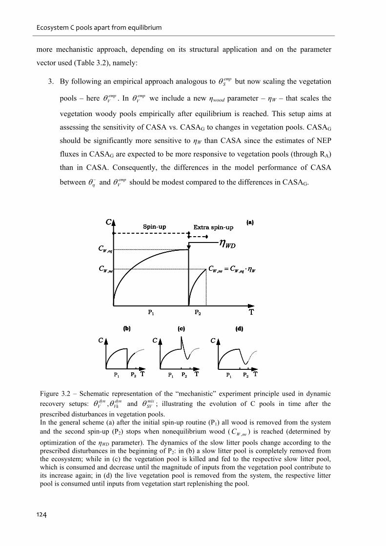
Ecosystem C pools apart from equilibrium
124
more mechanistic approach, depending on its structural application and on the parameter
vector used (Table 3.2), namely:
3. By following an empirical approach analogous to empS but now scaling the vegetation
pools – here empV . In emp
V we include a new ηwood parameter – ηW – that scales the
vegetation woody pools empirically after equilibrium is reached. This setup aims at
assessing the sensitivity of CASA vs. CASAG to changes in vegetation pools. CASAG
should be significantly more sensitive to ηW than CASA since the estimates of NEP
fluxes in CASAG are expected to be more responsive to vegetation pools (through RA)
than in CASA. Consequently, the differences in the model performance of CASA
between and emp
V should be modest compared to the differences in CASAG.
Spin-up Extra spin-up
TP1 P2
C
eqWC ,
neWC ,
WD
WeqWneW CC ,,
(a)
TP1 P2
C
(b)
TP1 P2
C
(c)
P1 P2
C
T
(d)
Spin-up Extra spin-up
TP1 P2
C
eqWC ,
neWC ,
WD
WeqWneW CC ,,
(a)Spin-up Extra spin-up
TP1 P2
C
eqWC ,
neWC ,
WD
WeqWneW CC ,,
Spin-up Extra spin-up
TP1 P2
C
eqWC ,
neWC ,
WD
WeqWneW CC ,,
(a)
TP1 P2
C
(b)
TP1 P2
C
(b)
TP1 P2
C
(c)
TP1 P2
C
(c)
P1 P2
C
T
(d)
P1 P2
C
T
(d)
Figure 3.2 – Schematic representation of the “mechanistic” experiment principle used in dynamic
recovery setups: dynV , dyn
Vk and mixSV ; illustrating the evolution of C pools in time after the
prescribed disturbances in vegetation pools. In the general scheme (a) after the initial spin-up routine (P1) all wood is removed from the system and the second spin-up (P2) stops when nonequilibrium wood ( neWC , ) is reached (determined by
optimization of the ηWD parameter). The dynamics of the slow litter pools change according to the prescribed disturbances in the beginning of P2: in (b) a slow litter pool is completely removed from the ecosystem; while in (c) the vegetation pool is killed and fed to the respective slow litter pool, which is consumed and decrease until the magnitude of inputs from the vegetation pool contribute to its increase again; in (d) the live vegetation pool is removed from the system, the respective litter pool is consumed until inputs from vegetation start replenishing the pool.
Materials and Methods
125
4. The first approach to relax both vegetation and soil pools from equilibrium is strictly
empirical. Here, in empSV , we optimize ηWL – this ηwood parameter scales the vegetation
woody and slow litter pools equally after the spin-up. This simultaneous and equal
scaling implies proportionality between woody and slow litter pools disequilibrium.
Additionally, nonequilibrium conditions in soil pools are prescribed by η’ that relaxes
the steady state in the microbial and slow soil pools (Figure 3.1). The role of empSV is
then to assess the impacts of nonsteady-state conditions in vegetation and litter pools
and in soil pools using a purely empirical approach.
5. Additionally, we implement a semi-mechanistic setup that allows the vegetation pools
to recover from prescribed disturbances – mixSV . In mix
SV , we introduce a new ηwood
parameter – ηWD – that prescribes a complete tree cut after spin-up completion (P1) and
allows a dynamic recovery during a second initialization routine (P2, Figure 3.2). At P1
the wood carbon pool (CW) which was in equilibrium ( eqWC , ) is removed (set to zero)
while leaves and roots are killed, but not removed from the system. This procedure is
not the same for all sites since the specific site history (see above) entails dynamics
that are mechanistically different from such general prescription. Hence: 1) in ES-ES1
we do not remove the killed trees from the system but we remove the surface pools,
due to its fire history; 2) in IT-PT1 we remove all the vegetation and surface litter
pools from the system, since the clear cut activities remove all surface litter; and 3)
since IT-Ro1 and IT-Ro2 are coppice sites the roots are not killed. The model is then
spun-up during a second spin-up phase (P2) which lasts until neWW CC , (Figure 3.2),
upon which nonequilibrium CW ( neWC , ) is estimated as:
WDeqWneW CC ,, , (3.1)
being ηWD parameterized during the optimization. During both spin-up phases – P1 and
P2 – the model simulations were performed with a mean year of drivers for the
observation years (Table 3.1). In the general dynamic prescription the coarse woody
debris is affected indirectly, through the complete reduction of C inputs from the wood
pool after P1 that dynamically increase during P2 (Figure 3.2d). The coarse root litter
pool experiences an immediate increase of C inputs after P1 and a decrease in early P2,
followed by a dynamic increase analogously to the coarse woody debris pool (Figure
3.2c). In the specific cases the dynamics are: 1) for ES-ES1 the slow litter pools
experience an immediate increase of C inputs after P1 and a decrease in early P2,
Ecosystem C pools apart from equilibrium
126
followed by dynamic increases as vegetation recovers and inputs carbon to the litter
pools (Figure 3.2c); 2) in IT-PT1 all surface litter pools re-start a spin-up from zero,
growing from vegetation inputs during P2 (Figure 3.2b); and 3) for IT-Ro1 and IT-Ro2
the only difference to the general case is that the coarse root litter dynamics are not
changed (the coarse woody debris follow Figure 3.2d). Further, η’ is also included in
the parameter vector, empirically relaxing the slow and microbial soil pools. Overall,
mixSV aims to reproduce the impacts of past vegetation disturbances following a semi-
mechanistic approach: through the dynamic prescription of ηWD and the heuristic
approach of η’.
6. In dynV , nonequilibrium conditions are solely prescribed through ηWD, which is
integrated in the parameter vector exactly as in the mixSV setup. Here, the occurrence of
nonsteady-state conditions in non-vegetation pools results only from changes in the
dynamics of C inputs from vegetation pools. It is the intent of dynV to test whether the
prescription of a dynamic disturbance recovery in a mechanistically consistent manner
is comparable to the model performance of semi-mechanistic and fully empirical
approaches.
7. The dynVk experiment builds on the dyn
V setup by adding a parameter that adjusts the
wood and coarse root turnover rates (kWR). The prescribed dynamics and implications
are identical to dynV . However, by adjusting the turnover rates of the slow vegetation
pools we seek to correct potential inconsistencies in model dynamics during the
second phase of the spin-up (P2, Figure 3.2). Despite the heuristic character of kWR, this
setup allows assessment as to whether the potential falsification of dynV might be due
to its fixed turnover rate.
Throughout the collection of parameter vectors we constantly include maximum energy to
mass conversion rates (ε* and *g ) and parameters that control the response curves of light use
efficiency and RH to climate and environmental drivers: optimum temperature for
photosynthesis (Topt); sensitivity of photosynthesis to water stress (Bwε); increase in soil
biological activity for a 10ºC increase in temperature (Q10); and RH sensitivity to water
availability (Aws) (for further details see Annex II).
Materials and Methods
127
3.3.4. Integration of vegetation pools in the model optimization
The model parameters in each setup are optimized through the minimization of the residual
sum of squares between modelled daily NEP estimates and daily integrals of eddy-covariance
measurements of CO2 fluxes (gC.m-2.d-1) [Aubinet et al., 2000]. The optimization is
performed individually for each parameter vector and for each ecosystem site (Table 3.1),
using the Levenberg-Marquardt algorithm [Levenberg, 1944; Marquardt, 1963]. The
integration of information related to wood biomass (CW, gC.m-2), above ground biomass
(AGB, gC.m-2) and wood NPP (NPPW – carbon accumulation in the wood pool – gC.m-2.yr-1)
in the cost function is performed where such data is available (Table 3.1 and Annex VI). The
observational data of vegetation pools was extracted from the Luyssaert et al. [2007] database
in sites where available, including observations of AGB, NPPW and CW for four sites used
(Table 3.1).
3.3.5. Statistical analysis
The model performance was evaluated independently per optimization by selected statistical
indicators according to Janssen and Heuberger [1995]: normalized average error (NAE);
variance ratio (VR); modelling efficiency (MEF); and correlation coefficient, (r2). The model
performance in estimating vegetation C pools was based on the normalized mean absolute
error (NMAE) (Annex III).
The comparisons between model performance statistics and optimized parameter values were
supported by the sign test [Sprent and Smeeton., 2001]. We tested the null hypothesis that the
median of the difference vector between two variables was zero, for a 5% significance level.
The sign test avoids: (i) the normal distribution assumption; and (ii) distribution symmetry; in
our case, relevant advantages over the t-test and the Wilcoxon signed rank test [Sprent and
Smeeton., 2001; Yang et al., 2004].
Further, the experimental design includes parameter vectors with different number of
parameters. In some cases, the improvements in model performance could also be originated
from the addition of extra free parameters to the parameter vector. To account for the
influences of the different sets of free parameters represented by the various model structures
we computed the Akaike information criterion (AIC) [Akaike, 1974] for each optimization:
PnAIC 2ˆlog 2 , (3.2)
where n is the number of observations, 2 is the mean sum of squares and P is the number of
free parameters in the model [Burnham and Anderson, 2004]. The computation of AIC relies
Ecosystem C pools apart from equilibrium
128
on arbitrary constants (Eq. 2) and its values can range from negative to positive through
several orders of magnitude. For easiness of interpretation we adopt the AIC scaling (Δθ)
suggested by [Burnham and Anderson, 2004]:
minAICAIC , (3.3)
where Δθ is the AIC scaling for a certain experiment θ for a given site, while AICθ is its
respective AIC value and AICmin is the minimum AIC of all the experiments for that site. The
parsimonious model is the one with the smaller AIC score and in this case is going to be the
model that yields a Δθ = 0.
Also, following the current experimental design, different factors (site, model version,
parameter vector and cost function type) could have contributed to the variability in both
model performance and optimized parameters. The identification of the main determinants of
variance of a variable was supported by n-way analysis of variance (ANOVA), 95%
confidence degree [Hogg and Ledolter, 1987].
3.4. Results and Discussion
3.4.1. Structural changes in the CASA model
The adjustments in the CASA model (CASAG, see Annex V) yield significant increases in the
sensitivity of ecosystem fluxes to vegetation pools as intended. Yet, the differences in model
performance for NEP between CASA and CASAG are not significant (Table 3.3), nor are the
differences in the optimized parameter – except between ε* and *g , as expected. The inter-
site variation in the carbon use efficiency (CUE=NPP/GPP) calculated by CASAG is well
within values reported by other studies [DeLucia et al., 2007; Litton et al., 2007] (see Annex
V). Further, the overall NPP GPP relationship follows a significant linear pattern, with a slope
closer to global values for optimizations considering multiple constraints approaches (for
details see Annex V). These results support the utilization of CASAG for the current
experiment; hence, further analyses refer to CASAG, except where indicated otherwise.
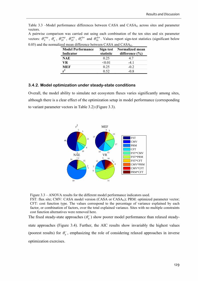
Results and Discussion
129
Table 3.3 –Model performance differences between CASA and CASAG across sites and parameter vectors. A pairwise comparison was carried out using each combination of the ten sites and six parameter
vectors: empS ,
, empSV , mix
SV , dynV and dyn
Vk . Values report sign-test statistics (significant below
0.05) and the normalized mean difference between CASA and CASAG. Model Performance Indicator
Sign test statistic
Normalized mean difference (%)
NAE 0.25 4.7 VR <0.01 -4.1 MEF 0.25 -0.2 r2 0.52 -0.8
3.4.2. Model optimization under steady-state conditions
Overall, the model ability to simulate net ecosystem fluxes varies significantly among sites,
although there is a clear effect of the optimization setup in model performance (corresponding
to variant parameter vectors in Table 3.2) (Figure 3.3).
48
610
4
21
55
r2
37
10 15
17
13
34MEF
16
59
52
1521
NAE5
13
5
6
51
43
210
VR
FSTCMVPRMCFTFST*CMVFST*PRMFST*CFTCMV*PRMCMV*CFTPRM*CFT
Figure 3.3 – ANOVA results for the different model performance indicators used. FST: flux site; CMV: CASA model version (CASA or CASAG); PRM: optimized parameter vector; CFT: cost function type. The values correspond to the percentage of variance explained by each factor, or combination of factors, over the total explained variance. Sites with no multiple constraints cost function alternatives were removed here.
The fixed steady-state approaches ( ) show poorer model performance than relaxed steady-
state approaches (Figure 3.4). Further, the AIC results show invariably the highest values
(poorest results) for , emphasizing the role of considering relaxed approaches in inverse
optimization exercises.
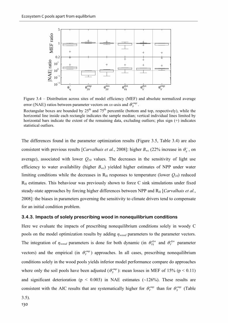
Ecosystem C pools apart from equilibrium
130
0.2
1
5
ME
F ra
tio
10−2
10−1
100
101
|NA
E| r
atio
θη − θ
SVemp θ
SVmix θ
Vkdyn θ
V dyn θ
V emp
Figure 3.4 – Distribution across sites of model efficiency (MEF) and absolute normalized average
error (|NAE|) ratios between parameter vectors on xx-axis and empS .
Rectangular boxes are bounded by 25th and 75th percentile (bottom and top, respectively), while the horizontal line inside each rectangle indicates the sample median; vertical individual lines limited by horizontal bars indicate the extent of the remaining data, excluding outliers; plus sign (+) indicates statistical outliers.
The differences found in the parameter optimization results (Figure 3.5, Table 3.4) are also
consistent with previous results [Carvalhais et al., 2008]: higher Bwε (22% increase in , on
average), associated with lower Q10 values. The decreases in the sensitivity of light use
efficiency to water availability (higher Bwε) yielded higher estimates of NPP under water
limiting conditions while the decreases in RH responses to temperature (lower Q10) reduced
RH estimates. This behaviour was previously shown to force C sink simulations under fixed
steady-state approaches by forcing higher differences between NPP and RH [Carvalhais et al.,
2008]: the biases in parameters governing the sensitivity to climate drivers tend to compensate
for an initial condition problem.
3.4.3. Impacts of solely prescribing wood in nonequilibrium conditions
Here we evaluate the impacts of prescribing nonequilibrium conditions solely in woody C
pools on the model optimization results by adding ηwood parameters to the parameter vectors.
The integration of ηwood parameters is done for both dynamic (in dynVk and dyn
V parameter
vectors) and the empirical (in empV ) approaches. In all cases, prescribing nonequilibrium
conditions solely in the wood pools yields inferior model performance compare do approaches
where only the soil pools have been adjusted ( empS ): mean losses in MEF of 15% (p < 0.11)
and significant deterioration (p < 0.003) in NAE estimates (~126%). These results are
consistent with the AIC results that are systematically higher for empV than for emp
S (Table
3.5).
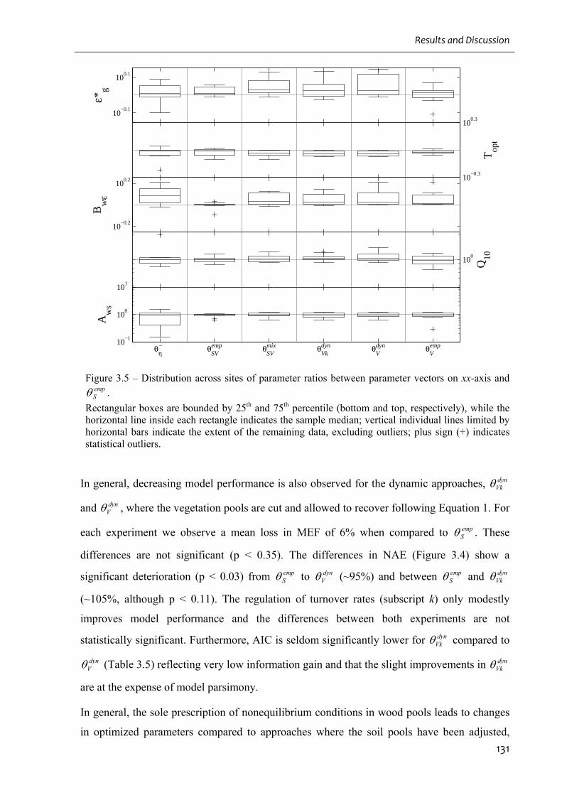
Results and Discussion
131
10−0.1
100.1
ε*g
10−0.3
100.3
Top
t
10−0.2
100.2
Bw
ε
100
Q10
10−1
100
101
Aw
s
θη − θ
SVemp θ
SVmix θ
Vkdyn θ
V dyn θ
V emp
Figure 3.5 – Distribution across sites of parameter ratios between parameter vectors on xx-axis and empS .
Rectangular boxes are bounded by 25th and 75th percentile (bottom and top, respectively), while the horizontal line inside each rectangle indicates the sample median; vertical individual lines limited by horizontal bars indicate the extent of the remaining data, excluding outliers; plus sign (+) indicates statistical outliers.
In general, decreasing model performance is also observed for the dynamic approaches, dynVk
and dynV , where the vegetation pools are cut and allowed to recover following Equation 1. For
each experiment we observe a mean loss in MEF of 6% when compared to empS . These
differences are not significant (p < 0.35). The differences in NAE (Figure 3.4) show a
significant deterioration (p < 0.03) from empS to dyn
V (~95%) and between empS and dyn
Vk
(~105%, although p < 0.11). The regulation of turnover rates (subscript k) only modestly
improves model performance and the differences between both experiments are not
statistically significant. Furthermore, AIC is seldom significantly lower for dynVk compared to
dynV (Table 3.5) reflecting very low information gain and that the slight improvements in dyn
Vk
are at the expense of model parsimony.
In general, the sole prescription of nonequilibrium conditions in wood pools leads to changes
in optimized parameters compared to approaches where the soil pools have been adjusted,
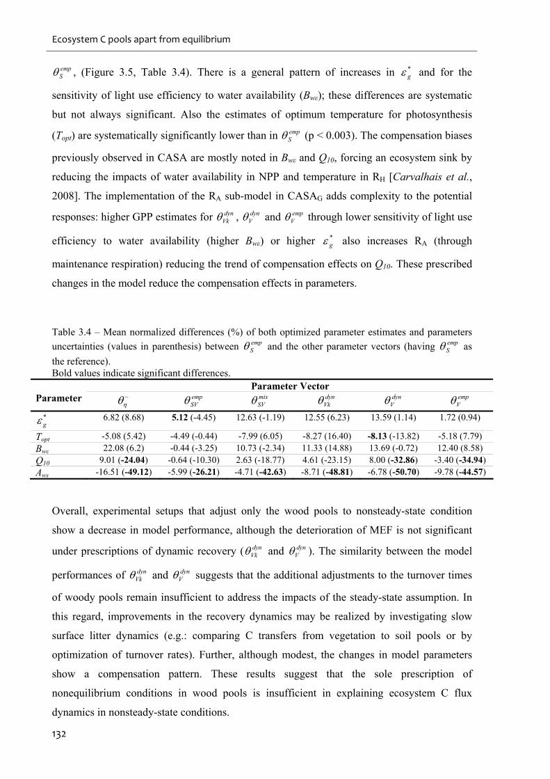
Ecosystem C pools apart from equilibrium
132
empS , (Figure 3.5, Table 3.4). There is a general pattern of increases in *
g and for the
sensitivity of light use efficiency to water availability (Bwε); these differences are systematic
but not always significant. Also the estimates of optimum temperature for photosynthesis
(Topt) are systematically significantly lower than in empS (p < 0.003). The compensation biases
previously observed in CASA are mostly noted in Bwε and Q10, forcing an ecosystem sink by
reducing the impacts of water availability in NPP and temperature in RH [Carvalhais et al.,
2008]. The implementation of the RA sub-model in CASAG adds complexity to the potential
responses: higher GPP estimates for dynVk , dyn
V and empV through lower sensitivity of light use
efficiency to water availability (higher Bwε) or higher *g also increases RA (through
maintenance respiration) reducing the trend of compensation effects on Q10. These prescribed
changes in the model reduce the compensation effects in parameters.
Table 3.4 – Mean normalized differences (%) of both optimized parameter estimates and parameters
uncertainties (values in parenthesis) between empS and the other parameter vectors (having emp
S as
the reference). Bold values indicate significant differences.
Parameter Vector Parameter
empSV mix
SV dynVk dyn
V empV
*g 6.82 (8.68) 5.12 (-4.45) 12.63 (-1.19) 12.55 (6.23) 13.59 (1.14) 1.72 (0.94)
Topt -5.08 (5.42) -4.49 (-0.44) -7.99 (6.05) -8.27 (16.40) -8.13 (-13.82) -5.18 (7.79)
Bwε 22.08 (6.2) -0.44 (-3.25) 10.73 (-2.34) 11.33 (14.88) 13.69 (-0.72) 12.40 (8.58)
Q10 9.01 (-24.04) -0.64 (-10.30) 2.63 (-18.77) 4.61 (-23.15) 8.00 (-32.86) -3.40 (-34.94)
Aws -16.51 (-49.12) -5.99 (-26.21) -4.71 (-42.63) -8.71 (-48.81) -6.78 (-50.70) -9.78 (-44.57)
Overall, experimental setups that adjust only the wood pools to nonsteady-state condition
show a decrease in model performance, although the deterioration of MEF is not significant
under prescriptions of dynamic recovery ( dynVk and dyn
V ). The similarity between the model
performances of dynVk and dyn
V suggests that the additional adjustments to the turnover times
of woody pools remain insufficient to address the impacts of the steady-state assumption. In
this regard, improvements in the recovery dynamics may be realized by investigating slow
surface litter dynamics (e.g.: comparing C transfers from vegetation to soil pools or by
optimization of turnover rates). Further, although modest, the changes in model parameters
show a compensation pattern. These results suggest that the sole prescription of
nonequilibrium conditions in wood pools is insufficient in explaining ecosystem C flux
dynamics in nonsteady-state conditions.
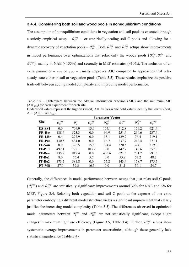
Results and Discussion
133
3.4.4. Considering both soil and wood pools in nonequilibrium conditions
The assumption of nonequilibrium conditions in vegetation and soil pools is executed through
a strictly empirical setup – empSV – or empirically scaling soil C pools and allowing for a
dynamic recovery of vegetation pools – mixSV . Both emp
SV and mixSV setups show improvements
in model performance over optimizations that relax only the woody pools ( dynVk , dyn
V and
empV ); mainly in NAE (~135%) and secondly in MEF estimates (~10%). The inclusion of an
extra parameter – ηWL or ηWD – usually improves AIC compared to approaches that relax
steady state either in soil or vegetation pools (Table 3.5). These results emphasize the positive
trade-off between adding model complexity and improving model performance.
Table 3.5 – Differences between the Akaike information criterion (AIC) and the minimum AIC (AICmin) for each experiment for each site. Underlined values represent the highest (worst) AIC values while bold values identify the lowest (best) AIC (AIC = AICmin).
Parameter Vector Site emp
S emp
SV mixSV dyn
V dynVk emp
V
ES-ES1 0.0 709.9 13.0 164.1 412.8 159.2 621.4 FR-Hes 188.6 523.3 0.0 94.9 251.6 260.6 237.6 FR-LBr 0.4 277.9 0.0 15.1 129.2 76.4 219.1 FR-Pue 130.5 434.0 0.0 16.7 237.7 242.4 271.1 IT-Non 0.0 376.5 55.6 174.4 320.5 324.1 319.0 IT-PT1 492.1 778.1 103.2 0.0 142.7 140.6 557.9 IT-Ren 235.9 919.4 0.0 405.6 621.5 731.2 891.5 IT-Ro1 8.0 76.4 5.7 0.0 55.8 53.2 48.2 IT-Ro2 173.2 581.8 0.0 55.2 143.4 158.7 175.7 PT-Mi1 27.0 39.3 16.5 0.0 31.1 30.1 24.7
Generally, the differences in model performance between setups that just relax soil C pools
( empS ) and emp
SV are statistically significant: improvements around 32% for NAE and 6% for
MEF, Figure 3.4. Relaxing both vegetation and soil C pools at the expense of one extra
parameter embodying a different model structure yields a significant improvement that clearly
justifies the increasing model complexity (Table 3.5). The differences observed in optimized
model parameters between empS and emp
SV are not statistically significant, except slight
changes in maximum light use efficiency (Figure 3.5, Table 3.4). Further, empSV setups show
systematic average improvements in parameter uncertainties, although these generally lack
statistical significance (Table 3.4).
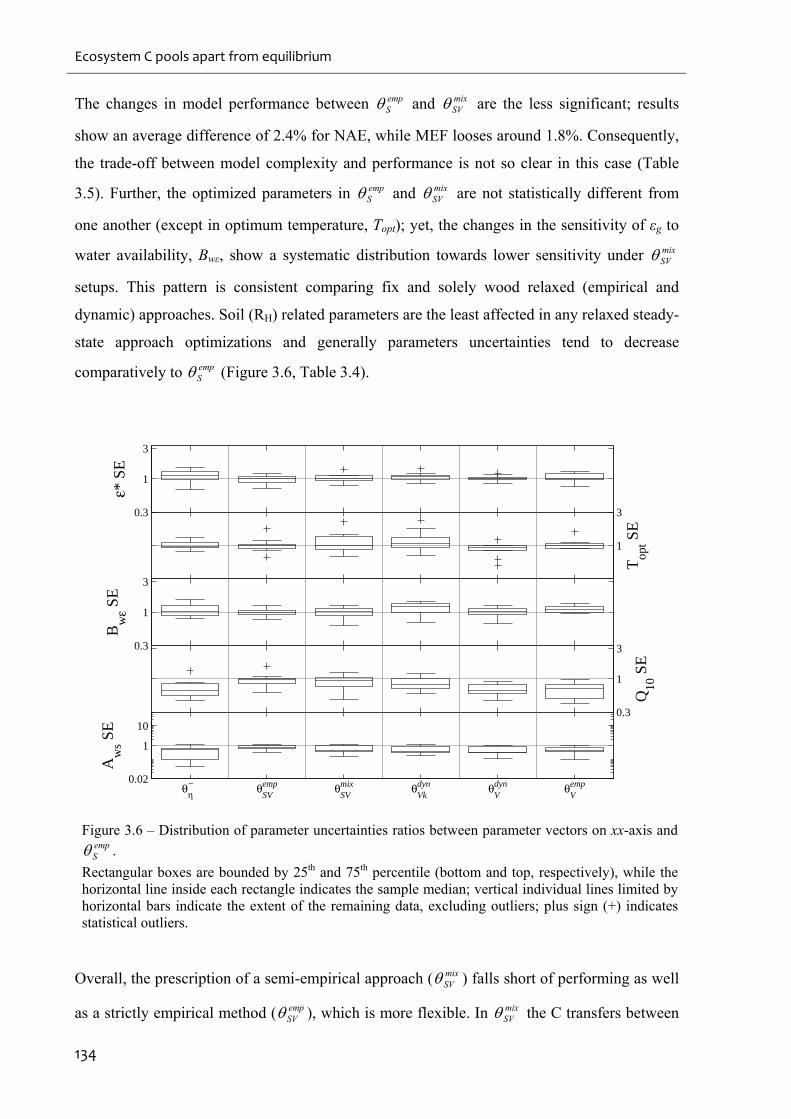
Ecosystem C pools apart from equilibrium
134
The changes in model performance between empS and mix
SV are the less significant; results
show an average difference of 2.4% for NAE, while MEF looses around 1.8%. Consequently,
the trade-off between model complexity and performance is not so clear in this case (Table
3.5). Further, the optimized parameters in empS and mix
SV are not statistically different from
one another (except in optimum temperature, Topt); yet, the changes in the sensitivity of εg to
water availability, Bwε, show a systematic distribution towards lower sensitivity under mixSV
setups. This pattern is consistent comparing fix and solely wood relaxed (empirical and
dynamic) approaches. Soil (RH) related parameters are the least affected in any relaxed steady-
state approach optimizations and generally parameters uncertainties tend to decrease
comparatively to empS (Figure 3.6, Table 3.4).
0.3
1
3
ε* S
E
1
3
Top
t SE
0.3
1
3
Bw
ε SE
0.3
1
3Q
10 S
E
0.02
1
10
Aw
s SE
θη − θ
SVemp θ
SVmix θ
Vkdyn θ
V dyn θ
V emp
Figure 3.6 – Distribution of parameter uncertainties ratios between parameter vectors on xx-axis and empS .
Rectangular boxes are bounded by 25th and 75th percentile (bottom and top, respectively), while the horizontal line inside each rectangle indicates the sample median; vertical individual lines limited by horizontal bars indicate the extent of the remaining data, excluding outliers; plus sign (+) indicates statistical outliers.
Overall, the prescription of a semi-empirical approach ( mixSV ) falls short of performing as well
as a strictly empirical method ( empSV ), which is more flexible. In mix
SV the C transfers between
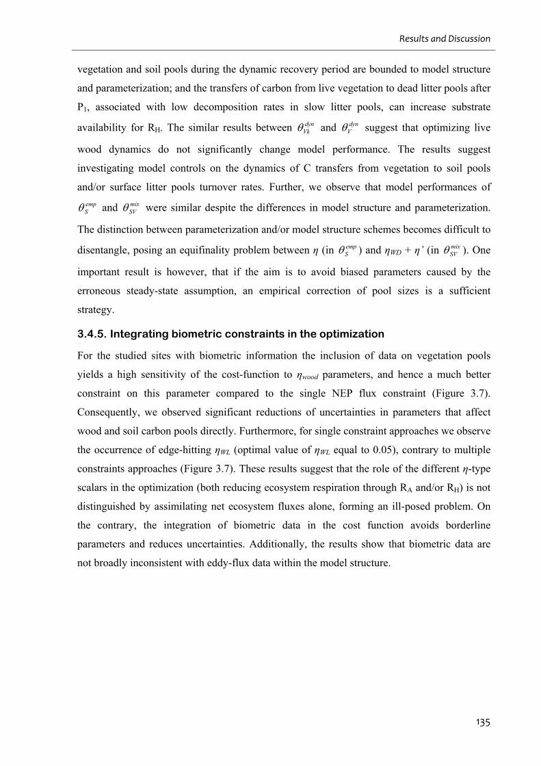
Results and Discussion
135
vegetation and soil pools during the dynamic recovery period are bounded to model structure
and parameterization; and the transfers of carbon from live vegetation to dead litter pools after
P1, associated with low decomposition rates in slow litter pools, can increase substrate
availability for RH. The similar results between dynVk and dyn
V suggest that optimizing live
wood dynamics do not significantly change model performance. The results suggest
investigating model controls on the dynamics of C transfers from vegetation to soil pools
and/or surface litter pools turnover rates. Further, we observe that model performances of
empS and mix
SV were similar despite the differences in model structure and parameterization.
The distinction between parameterization and/or model structure schemes becomes difficult to
disentangle, posing an equifinality problem between η (in empS ) and ηWD + η’ (in mix
SV ). One
important result is however, that if the aim is to avoid biased parameters caused by the
erroneous steady-state assumption, an empirical correction of pool sizes is a sufficient
strategy.
3.4.5. Integrating biometric constraints in the optimization
For the studied sites with biometric information the inclusion of data on vegetation pools
yields a high sensitivity of the cost-function to ηwood parameters, and hence a much better
constraint on this parameter compared to the single NEP flux constraint (Figure 3.7).
Consequently, we observed significant reductions of uncertainties in parameters that affect
wood and soil carbon pools directly. Furthermore, for single constraint approaches we observe
the occurrence of edge-hitting ηWL (optimal value of ηWL equal to 0.05), contrary to multiple
constraints approaches (Figure 3.7). These results suggest that the role of the different η-type
scalars in the optimization (both reducing ecosystem respiration through RA and/or RH) is not
distinguished by assimilating net ecosystem fluxes alone, forming an ill-posed problem. On
the contrary, the integration of biometric data in the cost function avoids borderline
parameters and reduces uncertainties. Additionally, the results show that biometric data are
not broadly inconsistent with eddy-flux data within the model structure.
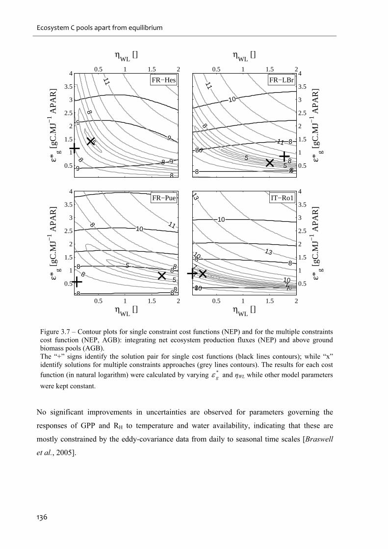
Ecosystem C pools apart from equilibrium
136
9
9
99
58
8
8
8
11
ηWL
[]ε*
g [gC
.MJ−
1 APA
R]
FR−Hes
0.5 1 1.5 2
0.5
1
1.5
2
2.5
3
3.5
4
88
8 8
10
55
8
8
8
8
11
11
ηWL
[]
ε*g [
gC.M
J−1 A
PAR
]
FR−LBr
0.5 1 1.5 2
0.5
1
1.5
2
2.5
3
3.5
4
8 8
8 8
10
5
5
8
88
8
11
ηWL
[]
ε*g [
gC.M
J−1 A
PAR
]
FR−Pue
0.5 1 1.5 2
0.5
1
1.5
2
2.5
3
3.5
4
8 8
8 8
10
7
7
7
7
10
1010
13
13
ηWL
[]ε*
g [gC
.MJ−
1 APA
R]
IT−Ro1
0.5 1 1.5 2
0.5
1
1.5
2
2.5
3
3.5
4
Figure 3.7 – Contour plots for single constraint cost functions (NEP) and for the multiple constraints cost function (NEP, AGB): integrating net ecosystem production fluxes (NEP) and above ground biomass pools (AGB). The “+” signs identify the solution pair for single cost functions (black lines contours); while “x” identify solutions for multiple constraints approaches (grey lines contours). The results for each cost
function (in natural logarithm) were calculated by varying *g and ηWL while other model parameters
were kept constant.
No significant improvements in uncertainties are observed for parameters governing the
responses of GPP and RH to temperature and water availability, indicating that these are
mostly constrained by the eddy-covariance data from daily to seasonal time scales [Braswell
et al., 2005].
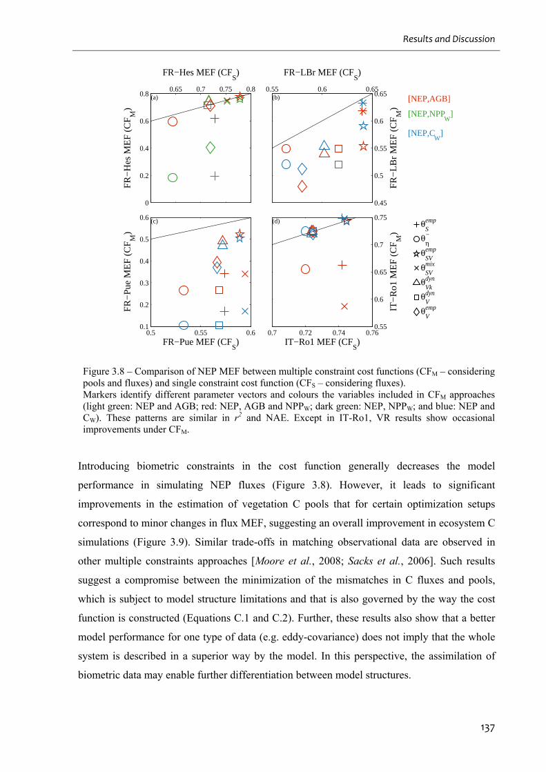
Results and Discussion
137
0.65 0.7 0.75 0.8
0
0.2
0.4
0.6
0.8
FR
−H
es M
EF
(C
FM
)
FR−Hes MEF (CFS)
(a)0.55 0.6 0.65
0.45
0.5
0.55
0.6
0.65
FR
−L
Br
ME
F (
CF
M)
FR−LBr MEF (CFS)
(b)
0.5 0.55 0.60.1
0.2
0.3
0.4
0.5
0.6
FR
−P
ue M
EF
(C
FM
)
FR−Pue MEF (CFS)
(c)
0.7 0.72 0.74 0.760.55
0.6
0.65
0.7
0.75
IT−
Ro1
ME
F (
CF
M)
IT−Ro1 MEF (CFS)
(d)
[NEP,AGB]
[NEP,NPPW
]
[NEP,CW
]
θV emp
θV dyn
θVkdyn
θSVmix
θSVemp
θS emp
θη −
Figure 3.8 – Comparison of NEP MEF between multiple constraint cost functions (CFM – considering pools and fluxes) and single constraint cost function (CFS – considering fluxes). Markers identify different parameter vectors and colours the variables included in CFM approaches (light green: NEP and AGB; red: NEP, AGB and NPPW; dark green: NEP, NPPW; and blue: NEP and CW). These patterns are similar in r2 and NAE. Except in IT-Ro1, VR results show occasional improvements under CFM.
Introducing biometric constraints in the cost function generally decreases the model
performance in simulating NEP fluxes (Figure 3.8). However, it leads to significant
improvements in the estimation of vegetation C pools that for certain optimization setups
correspond to minor changes in flux MEF, suggesting an overall improvement in ecosystem C
simulations (Figure 3.9). Similar trade-offs in matching observational data are observed in
other multiple constraints approaches [Moore et al., 2008; Sacks et al., 2006]. Such results
suggest a compromise between the minimization of the mismatches in C fluxes and pools,
which is subject to model structure limitations and that is also governed by the way the cost
function is constructed (Equations C.1 and C.2). Further, these results also show that a better
model performance for one type of data (e.g. eddy-covariance) does not imply that the whole
system is described in a superior way by the model. In this perspective, the assimilation of
biometric data may enable further differentiation between model structures.
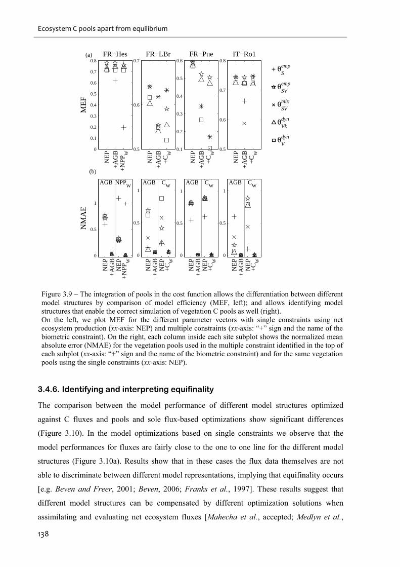
Ecosystem C pools apart from equilibrium
138
0
0.1
0.2
0.3
0.4
0.5
0.6
0.7
0.8
ME
F
FR−Hes
NE
P+
AG
B+
NPP
W
0.5
0.6
0.7FR−LBr
NE
P+
AG
B+
CW
0.1
0.2
0.3
0.4
0.5
0.6FR−Pue
NE
P+
AG
B+
CW
0.5
0.6
0.7
0.8IT−Ro1
NE
P+
AG
B+
CW
θV dyn
θVkdyn
θSVmix
θSVemp
θS emp
0
0.5
1
NM
AE
AGB NPPW
NE
P+
AG
BN
EP
+N
PPW
0
0.5
1
AGB CW
NE
P+
AG
BN
EP
+C
W
0
0.5
1
AGB CW
NE
P+
AG
BN
EP
+C
W
0
0.5
1
AGB CW
NE
P+
AG
BN
EP
+C
W
(a)
(b)
Figure 3.9 – The integration of pools in the cost function allows the differentiation between different model structures by comparison of model efficiency (MEF, left); and allows identifying model structures that enable the correct simulation of vegetation C pools as well (right). On the left, we plot MEF for the different parameter vectors with single constraints using net ecosystem production (xx-axis: NEP) and multiple constraints (xx-axis: “+” sign and the name of the biometric constraint). On the right, each column inside each site subplot shows the normalized mean absolute error (NMAE) for the vegetation pools used in the multiple constraint identified in the top of each subplot (xx-axis: “+” sign and the name of the biometric constraint) and for the same vegetation pools using the single constraints (xx-axis: NEP).
3.4.6. Identifying and interpreting equifinality
The comparison between the model performance of different model structures optimized
against C fluxes and pools and sole flux-based optimizations show significant differences
(Figure 3.10). In the model optimizations based on single constraints we observe that the
model performances for fluxes are fairly close to the one to one line for the different model
structures (Figure 3.10a). Results show that in these cases the flux data themselves are not
able to discriminate between different model representations, implying that equifinality occurs
[e.g. Beven and Freer, 2001; Beven, 2006; Franks et al., 1997]. These results suggest that
different model structures can be compensated by different optimization solutions when
assimilating and evaluating net ecosystem fluxes [Mahecha et al., accepted; Medlyn et al.,
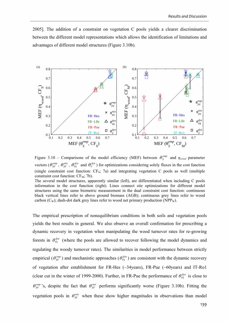
Results and Discussion
139
2005]. The addition of a constraint on vegetation C pools yields a clearer discrimination
between the different model representations which allows the identification of limitations and
advantages of different model structures (Figure 3.10b).
0.1 0.2 0.3 0.4 0.5 0.6 0.70.1
0.2
0.3
0.4
0.5
0.6
0.7
0.8
MEF (θS emp, CF
S)
ME
F (η
woo
d, CF S)
θV dyn
θVkdyn
θSVmix
θSVemp
IT−Ro1
FR−Pue
FR−LBr
FR−Hes
0.1 0.2 0.3 0.4 0.5 0.6 0.70.1
0.2
0.3
0.4
0.5
0.6
0.7
0.8
MEF (θS emp, CF
M)
ME
F (η
woo
d, CF M
)θ
V dyn
θVkdyn
θSVmix
θSVemp
IT−Ro1
FR−Pue
FR−LBr
FR−Hes
(a) (b)
Figure 3.10 – Comparisons of the model efficiency (MEF) between empS and ηwood parameter
vectors ( empSV , mix
SV , dynVk and dyn
V ) for optimizations considering solely fluxes in the cost function
(single constraint cost function: CFS; 7a) and integrating vegetation C pools as well (multiple constraint cost function: CFM; 7b). The several model structures, apparently similar (left), are differentiated when including C pools information in the cost function (right). Lines connect site optimizations for different model structures using the same biometric measurement in the dual constraint cost function: continuous black vertical lines refer to above ground biomass (AGB); continuous grey lines refer to wood carbon (CW); dash-dot dark grey lines refer to wood net primary production (NPPW).
The empirical prescription of nonequilibrium conditions in both soils and vegetation pools
yields the best results in general. We also observe an overall confirmation for prescribing a
dynamic recovery in vegetation when manipulating the wood turnover rates for re-growing
forests in dynVk (where the pools are allowed to recover following the model dynamics and
regulating the woody turnover rates). The similarities in model performance between strictly
empirical ( empSV ) and mechanistic approaches ( dyn
Vk ) are consistent with the dynamic recovery
of vegetation after establishment for FR-Hes (~34years), FR-Pue (~60years) and IT-Ro1
(clear cut in the winter of 1999-2000). Further, in FR-Pue the performance of dynVk is close to
empSV ’s, despite the fact that mix
SV performs significantly worse (Figure 3.10b). Fitting the
vegetation pools in mixSV when these show higher magnitudes in observations than model
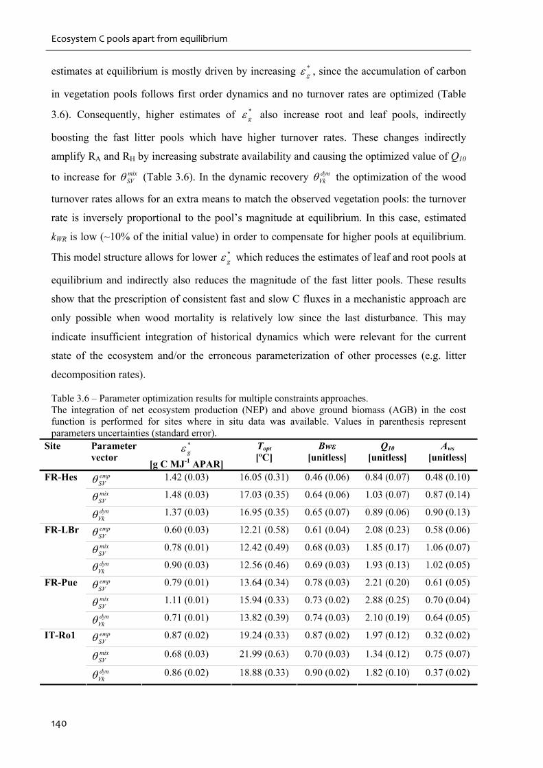
Ecosystem C pools apart from equilibrium
140
estimates at equilibrium is mostly driven by increasing *g , since the accumulation of carbon
in vegetation pools follows first order dynamics and no turnover rates are optimized (Table
3.6). Consequently, higher estimates of *g also increase root and leaf pools, indirectly
boosting the fast litter pools which have higher turnover rates. These changes indirectly
amplify RA and RH by increasing substrate availability and causing the optimized value of Q10
to increase for mixSV (Table 3.6). In the dynamic recovery dyn
Vk the optimization of the wood
turnover rates allows for an extra means to match the observed vegetation pools: the turnover
rate is inversely proportional to the pool’s magnitude at equilibrium. In this case, estimated
kWR is low (~10% of the initial value) in order to compensate for higher pools at equilibrium.
This model structure allows for lower *g which reduces the estimates of leaf and root pools at
equilibrium and indirectly also reduces the magnitude of the fast litter pools. These results
show that the prescription of consistent fast and slow C fluxes in a mechanistic approach are
only possible when wood mortality is relatively low since the last disturbance. This may
indicate insufficient integration of historical dynamics which were relevant for the current
state of the ecosystem and/or the erroneous parameterization of other processes (e.g. litter
decomposition rates).
Table 3.6 – Parameter optimization results for multiple constraints approaches. The integration of net ecosystem production (NEP) and above ground biomass (AGB) in the cost function is performed for sites where in situ data was available. Values in parenthesis represent parameters uncertainties (standard error).
Site Parameter vector
*g
[g C MJ-1 APAR]
Topt [ºC]
Bwε [unitless]
Q10 [unitless]
Aws [unitless]
empSV 1.42 (0.03) 16.05 (0.31) 0.46 (0.06) 0.84 (0.07) 0.48 (0.10)
mixSV 1.48 (0.03) 17.03 (0.35) 0.64 (0.06) 1.03 (0.07) 0.87 (0.14)
FR-Hes
dynVk 1.37 (0.03) 16.95 (0.35) 0.65 (0.07) 0.89 (0.06) 0.90 (0.13)
empSV 0.60 (0.03) 12.21 (0.58) 0.61 (0.04) 2.08 (0.23) 0.58 (0.06)
mixSV 0.78 (0.01) 12.42 (0.49) 0.68 (0.03) 1.85 (0.17) 1.06 (0.07)
FR-LBr
dynVk 0.90 (0.03) 12.56 (0.46) 0.69 (0.03) 1.93 (0.13) 1.02 (0.05)
empSV 0.79 (0.01) 13.64 (0.34) 0.78 (0.03) 2.21 (0.20) 0.61 (0.05)
mixSV 1.11 (0.01) 15.94 (0.33) 0.73 (0.02) 2.88 (0.25) 0.70 (0.04)
FR-Pue
dynVk 0.71 (0.01) 13.82 (0.39) 0.74 (0.03) 2.10 (0.19) 0.64 (0.05)
empSV 0.87 (0.02) 19.24 (0.33) 0.87 (0.02) 1.97 (0.12) 0.32 (0.02)
mixSV 0.68 (0.03) 21.99 (0.63) 0.70 (0.03) 1.34 (0.12) 0.75 (0.07)
IT-Ro1
dynVk 0.86 (0.02) 18.88 (0.33) 0.90 (0.02) 1.82 (0.10) 0.37 (0.02)
Results and Discussion
141
The inability of certain model structures to match both the observed carbon fluxes and pools is
significantly site dependent. In general the best results emerge from strictly empirical
approaches ( empSV ) although the prescription of site-specific recovery dynamics also yields
comparable modelling efficiencies (Figure 3.10). These results suggest the value of empirical
approaches as benchmarks against which more mechanistic approaches can be compared. The
consideration of multiple constraints highlights the limitations of forcing equilibrium solely
on soil (Figure 3.11a) or on vegetation (Figure 3.11b) pools. The prescription of a recovery
from a disturbance on vegetation (Figure 3.11c) show similar results to the empirical
relaxation on both types of pools (Figure 3.11d). These results highlight a multiple constraints
approach ability to exclude model representations such as empS and emp
V setups based on
significant reductions in MEF. The results also show a strong similarity in model efficiency
between the empirical relaxation of vegetation and soil pools ( empSV ) and the dyn
Vk setup. These
results emphasize the indirect role of the vegetation recovery mechanisms on nonsteady-state
conditions of ecosystems [Nabuurs, 2004]. In this case, the reduction of carbon inputs in the
ecosystem caused by the removal of the vegetation pool in the past is translated in
nonequilibrium conditions in both vegetation and soil level pools.
If inconsistencies between different types of observational data exist – in this case pools and
fluxes – these may hamper multiple constraints approaches. The presence of incompatible
measurements of fluxes and pools can bias parameters and/or can erroneously falsify or
corroborate model structures. In this regard, the consideration of basic rules for data
consistency checks is key [e.g. Luyssaert et al., 2007; Luyssaert et al., 2009]. In addition, we
recognize an increasing importance in addressing issues of data representation: 1) comparable
geographic coverage of flux and biometric data; and 2) correspondence between ecosystems
modelled and observed C pools. Further, information on uncertainty of different data sources
provides information about how constraining the measurements are, and can be indicative of
how mutually exclusive (or not) are different sets of observations.
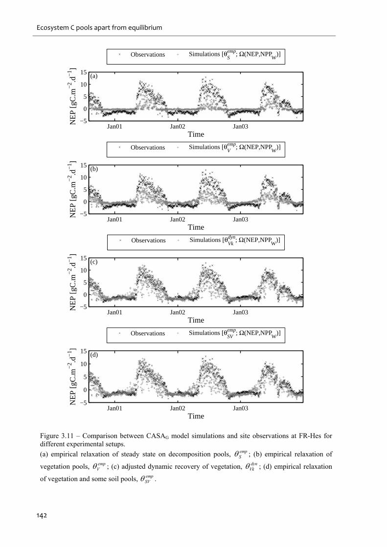
Ecosystem C pools apart from equilibrium
142
Jan01 Jan02 Jan03−5
0
5
10
15
Time
NE
P [g
C.m
−2 .d
−1 ]
(a)
Observations Simulations [θS emp; Ω(NEP,NPP
W)]
Jan01 Jan02 Jan03−5
0
5
10
15
Time
NE
P [g
C.m
−2 .d
−1 ]
(b)
Observations Simulations [θV emp; Ω(NEP,NPP
W)]
Jan01 Jan02 Jan03−5
0
5
10
15
Time
NE
P [g
C.m
−2 .d
−1 ]
(c)
Observations Simulations [θVkdyn; Ω(NEP,NPP
W)]
Jan01 Jan02 Jan03−5
0
5
10
15
Time
NE
P [g
C.m
−2 .d
−1 ]
(d)
Observations Simulations [θSVemp; Ω(NEP,NPP
W)]
Figure 3.11 – Comparison between CASAG model simulations and site observations at FR-Hes for different experimental setups.
(a) empirical relaxation of steady state on decomposition pools, empS ; (b) empirical relaxation of
vegetation pools, empV ; (c) adjusted dynamic recovery of vegetation, dyn
Vk ; (d) empirical relaxation
of vegetation and some soil pools, empSV .
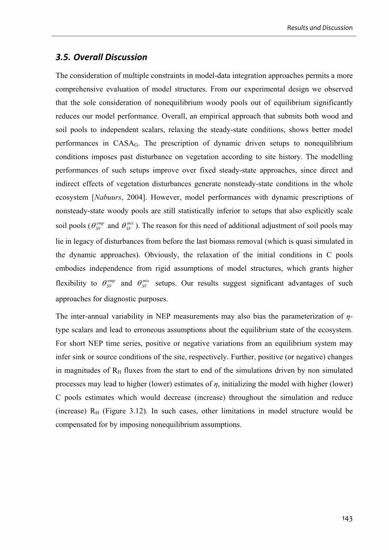
Results and Discussion
143
3.5. Overall Discussion
The consideration of multiple constraints in model-data integration approaches permits a more
comprehensive evaluation of model structures. From our experimental design we observed
that the sole consideration of nonequilibrium woody pools out of equilibrium significantly
reduces our model performance. Overall, an empirical approach that submits both wood and
soil pools to independent scalars, relaxing the steady-state conditions, shows better model
performances in CASAG. The prescription of dynamic driven setups to nonequilibrium
conditions imposes past disturbance on vegetation according to site history. The modelling
performances of such setups improve over fixed steady-state approaches, since direct and
indirect effects of vegetation disturbances generate nonsteady-state conditions in the whole
ecosystem [Nabuurs, 2004]. However, model performances with dynamic prescriptions of
nonsteady-state woody pools are still statistically inferior to setups that also explicitly scale
soil pools ( empSV and mix
SV ). The reason for this need of additional adjustment of soil pools may
lie in legacy of disturbances from before the last biomass removal (which is quasi simulated in
the dynamic approaches). Obviously, the relaxation of the initial conditions in C pools
embodies independence from rigid assumptions of model structures, which grants higher
flexibility to empSV and mix
SV setups. Our results suggest significant advantages of such
approaches for diagnostic purposes.
The inter-annual variability in NEP measurements may also bias the parameterization of η-
type scalars and lead to erroneous assumptions about the equilibrium state of the ecosystem.
For short NEP time series, positive or negative variations from an equilibrium system may
infer sink or source conditions of the site, respectively. Further, positive (or negative) changes
in magnitudes of RH fluxes from the start to end of the simulations driven by non simulated
processes may lead to higher (lower) estimates of η, initializing the model with higher (lower)
C pools estimates which would decrease (increase) throughout the simulation and reduce
(increase) RH (Figure 3.12). In such cases, other limitations in model structure would be
compensated for by imposing nonequilibrium assumptions.
Ecosystem C pools apart from equilibrium
144
1000 20000
1000
2000
3000
4000
5000
6000
Time (days)
Wood pool
1000 20000
500
1000
1500
Time (days)
Root pool
1000 20000
500
1000
1500
Time (days)
Leaf pool
1000 20000
500
1000
1500
2000
2500
3000
3500
Time (days)
Slow litter pool
1000 20000
500
1000
1500
2000
Time (days)Fast litter pool
1000 20000
50
100
150
200
250
300
350
Time (days)
Microbial pool
1000 20000
500
1000
1500
2000
2500
3000
3500
Time (days)
Slow pool
1000 20000
200
400
600
800
Time (days)
Old pool
FR−Pue
θSV
emp
θSV
mix
θVk
dyn
Figure 3.12 – Development of vegetation and soil C pools in FR-Pue for three experimental setups.
These consider: empirically relaxing pools ( empSV ); allowing for a dynamic recovery of vegetation
pools and prescribing and empirical distance to equilibrium in soil pools ( mixSV ); and simulating non
equilibrium conditions solely in vegetation pools, allowing recovery and regulating its turnover rates
( dynVk ).
The assimilation of both C fluxes and pools in the model-data integration approach may
degrade our ability to correctly simulate NEP fluxes [Williams et al., 2005] but allows the
identification of model structures unable to handle both sources of information. Multiple
constraints approaches allow the identification of model structures able to conciliate fast
fluxes (eddy-covariance) with long term integral of vegetation slow fluxes (biometric
measurements). The contribution to the equifinality problem may be undermined by
uncertainty in sporadic measurements of vegetation C pools; or by inconsistencies between
measurements and model representation of such pools; as well as by the lack of information
concerning site disturbance history. Further, we should acknowledge that in general errors
and/or biases in eddy-covariance measurements such as lack of energy balance closure
Overall Discussion
145
[Wilson et al., 2002] or errors in nocturnal measurements [e.g. Van Gorsel et al., 2007] can
influence parameter estimation. We suspect that some of the problems in simulating both
fluxes and pools for some sites may result from the simplified and uncalibrated RA model.
Integration of RA (or ecosystem respiration) data in future studies should help address these
problems. Other sources of data such as the integration of routine measurements of annual
wood increments at site level, by forest inventories or tree rings measurements, could also
contribute to efficient new constraints on annual integrals and inter-annual variability in
vegetation carbon assimilation.
Overall, model structures should be able to be confronted with multiple sources of data
relevant to the simulated dynamics. Although the consideration of a more complex model –
CASAG versus CASA – may violate the parsimony principle, it entails the possibility to
further assimilate new observational constraints. As expected, the model performances and
parameter optimization vary with model structure and cost function constraints at the site
level, although not all parameters are equally affected [Sacks et al., 2006]. Here, relating
different model structures with site history information may corroborate the different
simulation dynamics assumed and the mechanisms behind parameters change. Generally,
limitations in simulating dynamic approaches can be addressed with by more appropriate or
flexible model structures and better prescription of site specific disturbance dynamics. The
apparent limitations in our diagnostic ability may be further addressed by investigating long
term partitioning and transfers of C among the different ecosystem pools from
chronosequences.
3.6. Conclusions
We demonstrate that nonequilibrium assumptions of the vegetation pools alone are
insufficient for simulating NEP fluxes in nonsteady-state ecosystems. Consequently, the
relaxation of equilibrium conditions should be allowed on the full range of pools influencing
ecosystem C fluxes. The dynamics that follow the past disturbance of the vegetation pools
entail direct and indirect effects on whole ecosystem carbon balance. Yet, the ability of
representing these dynamics is significantly site dependent, supporting the empirical
relaxation of equilibrium conditions in ecosystem carbon pools.
We establish an assimilation scheme for information of vegetation carbon pool by including
biometric data in the optimization cost function. The trade-off between model performance in
ecosystem fluxes estimates and vegetation pools estimates highlights model structural
limitations. Further, demarked distinctions between different model structures are observed
Ecosystem C pools apart from equilibrium
146
when integrating both sources of information – fluxes and pools – in the cost function,
contrasting with similar performance results when constraining the assimilation scheme solely
with C fluxes. Our results suggest that multiple constraints in model-data integration
approaches provide a means for resolving or reducing equifinality issues. In this regard,
further model improvements could be gained from the consideration of separate ecosystem
flux components as well as of water and energy fluxes. Further, these results suggest that the
assimilation of biomass information from satellite remote sensing could support a more
comprehensive characterization of terrestrial ecosystems at larger spatial scales.
Acknowledgements
We are grateful to Marco Correia, Martin Jung, Gitta Lasslop, Mirco Migliavacca,
Christopher Neigh, Wouter Peters and Enrico Tomelleri for very helpful comments on the
manuscript. We are also very thankful to three anonymous reviewers for constructive
comments that significantly helped improving the manuscript. This work was supported by
the Portuguese Foundation for Science and Technology (FCT) under the MODNET project
(contract no. PTDC/AGR-CFL/69733/2006) and also by the CARBO-Extreme project (FP7-
ENV-2008-1-226701). NC acknowledges the support given by the Portuguese Foundation for
Science and Technology (FCT), the European Union under Operational Program “Science and
Innovation” (POCI 2010), PhD grant ref. SFRH/BD/6517/2001. MR is grateful to the Max-
Planck-Society for supporting the independent junior research group Biogeochemical Model-
Data Integration. Research leading to flux data and scientific insight was supported by the
CARBOEUROPE-IP project.
References
Akaike, H. (1974), New Look at Statistical-Model Identification, Ieee T Automat Contr, Ac19(6), 716-723.
Aubinet, M., A. Grelle, A. Ibrom, U. Rannik, J. Moncrieff, T. Foken, A. S. Kowalski, P. H. Martin, P. Berbigier, C. Bernhofer, R. Clement, J. Elbers, A. Granier, T. Grunwald, K. Morgenstern, K. Pilegaard, C. Rebmann, W. Snijders, R. Valentini, and T. Vesala (2000), Estimates of the annual net carbon and water exchange of forests: The EUROFLUX methodology, Advances in Ecological Research, 30, 113-175.
Barford, C. C., S. C. Wofsy, M. L. Goulden, J. W. Munger, E. H. Pyle, S. P. Urbanski, L. Hutyra, S. R. Saleska, D. Fitzjarrald, and K. Moore (2001), Factors controlling long- and short-term sequestration of atmospheric CO2 in a mid-latitude forest, Science, 294(5547), 1688-1691.
Beven, K. (1989), Changing Ideas in Hydrology - the Case of Physically-Based Models, J Hydrol, 105(1-2), 157-172.
References
147
Beven, K., and J. Freer (2001), Equifinality, data assimilation, and uncertainty estimation in mechanistic modelling of complex environmental systems using the GLUE methodology, J Hydrol, 249(1-4), 11-29.
Beven, K. (2006), A manifesto for the equifinality thesis, J Hydrol, 320(1-2), 18-36.
Bonan, G. B. (2008), Forests and Climate Change: Forcings, Feedbacks, and the Climate Benefits of Forests, Science, 320(5882), 1444-1449.
Braswell, B. H., W. J. Sacks, E. Linder, and D. S. Schimel (2005), Estimating diurnal to annual ecosystem parameters by synthesis of a carbon flux model with eddy covariance net ecosystem exchange observations, Global Change Biol, 11(2), 335-355.
Burnham, K. P., and D. R. Anderson (2004), Multimodel inference - understanding AIC and BIC in model selection, Sociological Methods & Research, 33(2), 261-304.
Cannell, M. G. R., and J. H. M. Thornley (2003), Ecosystem productivity is independent of some soil properties at equilibrium, Plant Soil, 257(1), 193-204.
Carvalhais, N., M. Reichstein, J. Seixas, G. J. Collatz, J. S. Pereira, P. Berbigier, A. Carrara, A. Granier, L. Montagnani, D. Papale, S. Rambal, M. J. Sanz, and R. Valentini (2008), Implications of the carbon cycle steady state assumption for biogeochemical modeling performance and inverse parameter retrieval, Global Biogeochem Cy, 22(2), doi:10.1029/2007GB003033.
Crout, N. M. J., D. Tarsitano, and A. T. Wood (2009), Is my model too complex? Evaluating model formulation using model reduction, Environmental Modelling & Software, 24(1), 1-7.
DeLucia, E. H., J. E. Drake, R. B. Thomas, and M. Gonzalez-Meler (2007), Forest carbon use efficiency: is respiration a constant fraction of gross primary production?, Global Change Biol, 13(6), 1157-1167.
Ferré, C., A. Leip, G. Matteucci, F. Previtali, and G. Seufert (2005), Impact of 40 years poplar cultivation on soil carbon stocks and greenhouse gas fluxes, Biogeosciences Discuss., 2(4), 897-931.
Field, C. B., J. T. Randerson, and C. M. Malmstrom (1995), Global Net Primary Production - Combining Ecology and Remote-Sensing, Remote Sens Environ, 51(1), 74-88.
Fox, A., M. Williams, A. D. Richardson, D. Cameron, J. H. Gove, T. Quaife, D. Ricciuto, M. Reichstein, E. Tomelleri, C. M. Trudinger, and M. T. Van Wijk (2009), The REFLEX project: Comparing different algorithms and implementations for the inversion of a terrestrial ecosystem model against eddy covariance data, Agr Forest Meteorol, 149(10), 1597-1615.
Franks, S. W., K. J. Beven, P. F. Quinn, and I. R. Wright (1997), On the sensitivity of soil-vegetation-atmosphere transfer (SVAT) schemes: Equifinality and the problem of robust calibration, Agr Forest Meteorol, 86(1-2), 63-75.
Friedlingstein, P., G. Joel, C. B. Field, and I. Y. Fung (1999), Toward an allocation scheme for global terrestrial carbon models, Global Change Biol, 5(7), 755-770.
Friedlingstein, P., P. Cox, R. Betts, L. Bopp, W. Von Bloh, V. Brovkin, P. Cadule, S. Doney, M. Eby, I. Fung, G. Bala, J. John, C. Jones, F. Joos, T. Kato, M. Kawamiya, W. Knorr, K. Lindsay, H. D. Matthews, T. Raddatz, P. Rayner, C. Reick, E. Roeckner, K. G. Schnitzler, R. Schnur, K. Strassmann, A. J. Weaver, C. Yoshikawa, and N. Zeng (2006), Climate-carbon cycle feedback analysis: Results from the (CMIP)-M-4 model intercomparison, J Climate, 19(14), 3337-3353.
Ecosystem C pools apart from equilibrium
148
Granier, A., N. Breda, B. Longdoz, P. Gross, and J. Ngao (2008), Ten years of fluxes and stand growth in a young beech forest at Hesse, North-eastern France, Ann for Sci, 65(7), doi:10.1051/forest:2008052
Heimann, M., and M. Reichstein (2008), Terrestrial ecosystem carbon dynamics and climate feedbacks, Nature, 451(7176), 289-292.
Hogg, R. V., and J. Ledolter (1987), Engineering Statistics, Macmillan, New York.
Janssen, P. H. M., and P. S. C. Heuberger (1995), Calibration of Process-Oriented Models, Ecol Model, 83(1-2), 55-66.
Jarvis, P., A. Rey, C. Petsikos, L. Wingate, M. Rayment, J. Pereira, J. Banza, J. David, F. Miglietta, M. Borghetti, G. Manca, and R. Valentini (2007), Drying and wetting of Mediterranean soils stimulates decomposition and carbon dioxide emission: the "Birch effect", Tree Physiol, 27(7), 929-940.
Joffre, R., S. Rambal, and F. Romane (1996), Local variations of ecosystem functions in Mediterranean evergreen oak woodland, Ann Sci Forest, 53(2-3), 561-570.
Knorr, W., and J. Kattge (2005), Inversion of terrestrial ecosystem model parameter values against eddy covariance measurements by Monte Carlo sampling, Global Change Biol, 11(8), 1333-1351.
Lauvaux, T., M. Uliasz, C. Sarrat, F. Chevallier, P. Bousquet, C. Lac, K. J. Davis, P. Ciais, A. S. Denning, and P. J. Rayner (2008), Mesoscale inversion: first results from the CERES campaign with synthetic data, Atmos Chem Phys, 8(13), 3459-3471.
Levenberg, K. (1944), A method for the solution of certain non-linear problems in least squares, Q. Appl. Math., 2, 164-168.
Litton, C. M., J. W. Raich, and M. G. Ryan (2007), Carbon allocation in forest ecosystems, Global Change Biol, 13(10), 2089-2109.
Loustau, D., P. Berbigier, A. Granier, Y. Brunet, T. Bariac, and R. Valentini (1999), Measuring the carbon balance of European forests: Case studies of the two French sites from the Euroflux Network: Short-term environmental controls on carbon dioxide flux in a boreal coniferous forest: Model computation compared with measurements by eddy, Comptes-rendus des Seances de l'Academie d'Agriculture de France, 85(6), 255–264.
Lugo, A. E., and S. Brown (1986), Steady-State Terrestrial Ecosystems and the Global Carbon-Cycle, Vegetatio, 68(2), 83-90.
Luo, Y. Q., L. H. Wu, J. A. Andrews, L. White, R. Matamala, K. V. R. Schafer, and W. H. Schlesinger (2001), Elevated CO2 differentiates ecosystem carbon processes: Deconvolution analysis of Duke Forest FACE data, Ecol Monogr, 71(3), 357-376.
Luyssaert, S., I. Inglima, M. Jung, A. D. Richardson, M. Reichsteins, D. Papale, S. L. Piao, E. D. Schulzes, L. Wingate, G. Matteucci, L. Aragao, M. Aubinet, C. Beers, C. Bernhoffer, K. G. Black, D. Bonal, J. M. Bonnefond, J. Chambers, P. Ciais, B. Cook, K. J. Davis, A. J. Dolman, B. Gielen, M. Goulden, J. Grace, A. Granier, A. Grelle, T. Griffis, T. Grunwald, G. Guidolotti, P. J. Hanson, R. Harding, D. Y. Hollinger, L. R. Hutyra, P. Kolar, B. Kruijt, W. Kutsch, F. Lagergren, T. Laurila, B. E. Law, G. Le Maire, A. Lindroth, D. Loustau, Y. Malhi, J. Mateus, M. Migliavacca, L. Misson, L. Montagnani, J. Moncrieff, E. Moors, J. W. Munger, E. Nikinmaa, S. V. Ollinger, G. Pita, C. Rebmann, O. Roupsard, N. Saigusa, M. J. Sanz, G. Seufert, C. Sierra, M. L. Smith, J. Tang, R. Valentini, T. Vesala, and I. A. Janssens (2007), CO2 balance of boreal, temperate, and tropical forests derived from a global database, Global Change Biol, 13(12), 2509-2537.
References
149
Luyssaert, S., E. D. Schulze, A. Borner, A. Knohl, D. Hessenmoller, B. E. Law, P. Ciais, and J. Grace (2008), Old-growth forests as global carbon sinks, Nature, 455(7210), 213-215.
Luyssaert, S., M. Reichstein, E. D. Schulze, I. A. Janssens, B. E. Law, D. Papale, D. Dragoni, M. L. Goulden, A. Granier, W. L. Kutsch, S. Linder, G. Matteucci, E. Moors, J. W. Munger, K. Pilegaard, M. Saunders, and E. M. Falge (2009), Toward a consistency cross-check of eddy covariance flux-based and biometric estimates of ecosystem carbon balance, Global Biogeochem Cy, 23, doi:10.1029/2008GB003377.
Mahecha, M. D., M. Reichstein, M. Jung, C. Beer, M. Brakhekke, N. Carvalhais, H. Lange, G. Le Maire, E. Moors, S. Zaehle, and S. I. Seneviratne (accepted), Comparing observations and process-based simulations of biosphere-atmosphere exchanges on multiple time scales, Journal of Geophysical Research - Biogeosciences.
Marquardt, D. W. (1963), An Algorithm for Least-Squares Estimation of Nonlinear Parameters, J Soc Ind Appl Math, 11(2), 431-441.
Medlyn, B. E., A. P. Robinson, R. Clement, and R. E. McMurtrie (2005), On the validation of models of forest CO2 exchange using eddy covariance data: some perils and pitfalls, Tree Physiol, 25(7), 839-857.
Migliavacca, M., M. Meroni, G. Manca, G. Matteucci, L. Montagnani, G. Grassi, T. Zenone, M. Teobaldelli, I. Goded, R. Colombo, and G. Seufert (2009), Seasonal and interannual patterns of carbon and water fluxes of a poplar plantation under peculiar eco-climatic conditions, Agr Forest Meteorol, 149(9), 1460-1476.
Montagnani, L., G. Manca, E. Canepa, E. Georgieva, M. Acosta, C. Feigenwinter, D. Janous, G. Kerschbaumer, A. Lindroth, L. Minach, S. Minerbi, M. Molder, M. Pavelka, G. Seufert, M. Zeri, and W. Ziegler (2009), A new mass conservation approach to the study of CO2 advection in an alpine forest, J. Geophys. Res.-Atmos., 114.
Moore, D. J. P., J. Hu, W. J. Sacks, D. S. Schimel, and R. K. Monson (2008), Estimating transpiration and the sensitivity of carbon uptake to water availability in a subalpine forest using a simple ecosystem process model informed by measured net CO2 and H2O fluxes, Agr Forest Meteorol, 148(10), 1467-1477.
Morales, P., M. T. Sykes, I. C. Prentice, P. Smith, B. Smith, H. Bugmann, B. Zierl, P. Friedlingstein, N. Viovy, S. Sabate, A. Sanchez, E. Pla, C. A. Gracia, S. Sitch, A. Arneth, and J. Ogee (2005), Comparing and evaluating process-based ecosystem model predictions of carbon and water fluxes in major European forest biomes, Global Change Biol, 11(12), 2211-2233.
Nabuurs, G.-J. (2004), Current Consequences of Past Actions: How to Separate Direct from Indirect, in The Global Carbon Cycle, edited by C. B. Field and M. R. Raupach, pp. 317-326, Island Press, Washington.
O'Neill, B. C., and N. B. Melnikov (2008), Learning about parameter and structural uncertainty in carbon cycle models, Climatic Change, 89(1-2), 23-44.
Odum, E. P. (1969), Strategy of Ecosystem Development, Science, 164(3877), 262-270.
Papale, D., M. Reichstein, M. Aubinet, E. Canfora, C. Bernhofer, W. Kutsch, B. Longdoz, S. Rambal, R. Valentini, T. Vesala, and D. Yakir (2006), Towards a standardized processing of Net Ecosystem Exchange measured with eddy covariance technique: algorithms and uncertainty estimation, Biogeosciences, 3, 571-583.
Pereira, J. S., J. A. Mateus, L. M. Aires, G. Pita, C. Pio, J. S. David, V. Andrade, J. Banza, T. S. David, T. A. Paco, and A. Rodrigues (2007), Net ecosystem carbon exchange in three contrasting Mediterranean ecosystems - the effect of drought, Biogeosciences, 4(5), 791-802.
Ecosystem C pools apart from equilibrium
150
Pietsch, S. A., and H. Hasenauer (2006), Evaluating the self-initialization procedure for large-scale ecosystem models, Global Change Biol, 12(9), 1658-1669.
Potter, C. S., J. T. Randerson, C. B. Field, P. A. Matson, P. M. Vitousek, H. A. Mooney, and S. A. Klooster (1993), Terrestrial Ecosystem Production - a Process Model-Based on Global Satellite and Surface Data, Global Biogeochem Cy, 7(4), 811-841.
Randerson, J. T., M. V. Thompson, C. M. Malmstrom, C. B. Field, and I. Y. Fung (1996), Substrate limitations for heterotrophs: Implications for models that estimate the seasonal cycle of atmospheric CO2, Global Biogeochem Cy, 10(4), 585-602.
Reichstein, M., E. Falge, D. Baldocchi, D. Papale, M. Aubinet, P. Berbigier, C. Bernhofer, N. Buchmann, T. Gilmanov, A. Granier, T. Grunwald, K. Havrankova, H. Ilvesniemi, D. Janous, A. Knohl, T. Laurila, A. Lohila, D. Loustau, G. Matteucci, T. Meyers, F. Miglietta, J. M. Ourcival, J. Pumpanen, S. Rambal, E. Rotenberg, M. Sanz, J. Tenhunen, G. Seufert, F. Vaccari, T. Vesala, D. Yakir, and R. Valentini (2005), On the separation of net ecosystem exchange into assimilation and ecosystem respiration: review and improved algorithm, Global Change Biol, 11(9), 1424-1439.
Rey, A., E. Pegoraro, V. Tedeschi, I. De Parri, P. G. Jarvis, and R. Valentini (2002), Annual variation in soil respiration and its components in a coppice oak forest in Central Italy, Global Change Biol, 8(9), 851-866.
Sacks, W. J., D. S. Schimel, R. K. Monson, and B. H. Braswell (2006), Model-data synthesis of diurnal and seasonal CO2 fluxes at Niwot Ridge, Colorado, Global Change Biol, 12(2), 240-259.
Santaren, D., P. Peylin, N. Viovy, and P. Ciais (2007), Optimizing a process-based ecosystem model with eddy-covariance flux measurements: A pine forest in southern France, Global Biogeochem Cy, 21(2), doi:10.1029/2006GB002834.
Schaefer, K., G. J. Collatz, P. Tans, A. S. Denning, I. Baker, J. Berry, L. Prihodko, N. Suits, and A. Philpott (2008), Combined Simple Biosphere/Carnegie-Ames-Stanford Approach terrestrial carbon cycle model, Journal of Geophysical Research, 113, doi:10.1029/2007JG000603.
Scholze, M., T. Kaminski, P. Rayner, W. Knorr, and R. Giering (2007), Propagating uncertainty through prognostic carbon cycle data assimilation system simulations, J. Geophys. Res.-Atmos., 112(D17), doi:10.1029/2007JD008642.
Sprent, P., and N. C. Smeeton. (2001), Applied Nonparametric Statistical Methods, Boca Raton.
Thornton, P. E., B. E. Law, H. L. Gholz, K. L. Clark, E. Falge, D. S. Ellsworth, A. H. Golstein, R. K. Monson, D. Hollinger, M. Falk, J. Chen, and J. P. Sparks (2002), Modeling and measuring the effects of disturbance history and climate on carbon and water budgets in evergreen needleleaf forests, Agr Forest Meteorol, 113(1-4), 185-222.
Van Gorsel, E., R. Leuning, H. A. Cleugh, H. Keith, and T. Suni (2007), Nocturnal carbon efflux: reconciliation of eddy covariance and chamber measurements using an alternative to the u(*)-threshold filtering technique, Tellus B, 59(3), 397-403.
Williams, M., P. A. Schwarz, B. E. Law, J. Irvine, and M. R. Kurpius (2005), An improved analysis of forest carbon dynamics using data assimilation, Global Change Biol, 11(1), 89-105.
Wilson, K., A. Goldstein, E. Falge, M. Aubinet, D. Baldocchi, P. Berbigier, C. Bernhofer, R. Ceulemans, H. Dolman, C. Field, A. Grelle, A. Ibrom, B. E. Law, A. Kowalski, T. Meyers, J.

References
151
Moncrieff, R. Monson, W. Oechel, J. Tenhunen, R. Valentini, and S. Verma (2002), Energy balance closure at FLUXNET sites, Agr Forest Meteorol, 113(1-4), 223-243.
Wutzler, T., and M. Reichstein (2007), Soils apart from equilibrium – consequences for soil carbon balance modelling, Biogeosciences, 4(1), 125-136.
Yang, Y. Q., R. A. Monserud, and S. M. Huang (2004), An evaluation of diagnostic tests and their roles in validating forest biometric models, Can J Forest Res, 34(3), 619-629.

153
Chapter 4 – Deciphering the Components of Regional Net
Ecosystem Fluxes Following a Bottom‐Up Approach for the
Iberian Peninsula
4.1. Summary
Quantification of ecosystem carbon pools is a fundamental requirement for estimating carbon
fluxes and for addressing the dynamics and responses of the terrestrial carbon cycle to
environmental drivers. The initial estimates of carbon pools in terrestrial carbon cycle models
often rely on the ecosystem steady-state assumption, leading to initial equilibrium conditions.
In this study, we investigate how trends and inter-annual variability in net ecosystem fluxes
are affected by initial nonsteady-state conditions. Further, we examine how modeled
ecosystem responses induced exclusively by the model drivers can be separated from the
initial conditions. For this, the Carnegie-Ames-Stanford Approach (CASA) model is
optimized at a set of European eddy-covariance sites, which support the parameterization of
regional simulations of ecosystem fluxes for the Iberian Peninsula, between 1982 and 2006.
The presented analysis stands on a credible model performance for a set of sites that well
represent the plant functional types and selected descriptors of climate and phenology present in
the Iberian region – except for a limited North-western area. The effects of initial conditions on
inter-annual variability and on trends, results mostly from the recovery of pools to equilibrium
conditions; which control most of the inter-annual variability (IAV) and both the magnitude
and sign of most of the trends. However, by removing the time series of pure model recovery
from the time series of the overall fluxes, we are able to retrieve estimates of inter-annual
variability and trends in net ecosystem fluxes that are quasi-independent from the initial
conditions. Such approach reduced the sensitivity of the net fluxes to initial conditions from
47% and 174% to -3% and 7%, for strong initial sink and source conditions, respectively.
With the aim to identify and improve understanding of the component fluxes that drive the
observed trends, the net ecosystem production (NEP) trends are decomposed into net primary
production (NPP) and heterotrophic respiration (RH) trends. The majority (~97%) of the
Upscaling ecosystem C fluxes for the Iberian Peninsula
154
positive trends in NEP is observed in regions where both NPP and RH fluxes show significant
increases, although the magnitude of NPP trends is higher. Analogously, ~83% of the
negative trends in NEP are also associated with negative trends in NPP. The spatial patterns of
NPP trends are mainly explained by the trends in fAPAR (r = 0.79) and are only marginally
explained by trends in temperature and water stress scalars (r = 0.10 and r = 0.25,
respectively). Further, we observe the significant role of substrate availability (r = 0.25) and
temperature (r = 0.23) in explaining the spatial patterns of trends in RH. These results
highlight the role of primary production in driving ecosystem fluxes.
Overall, our study illustrates an approach for removing the confounding effects of initial
conditions and emphasizes the need to decompose the ecosystem fluxes into its components
and drivers for more mechanistic interpretations of modelling results. We expect that our
results are not only specific for the CASA model since it incorporates concepts of ecosystem
functioning and modelling assumptions common to biogeochemical models. A direct
implication of these results is the ability of this approach to detect climate and phenology
induced trends regardless of the initial conditions.
4.2. Introduction
The quantification of terrestrial net ecosystem fluxes is of significant importance to the
understanding of the global carbon cycle [e.g. Heimann and Reichstein, 2008] and has been
the subject of active research [e.g. Ciais et al., 2000; Piao et al., 2009b]. In this regard,
model-data synthesis approaches have focused on the improvement of ecosystem fluxes
estimates through model structure development [e.g. Richardson et al., 2006], estimation of
parameters [e.g. Knorr and Kattge, 2005; Zaehle et al., 2005] and initial conditions [e.g.
Braswell et al., 2005; Carvalhais et al., 2008], adjustments in state variables [e.g. Jones et al.,
2004] and sensitivity to forcing variables [e.g. Abramowitz et al., 2008]. The wide assessment
of uncertainties in the different modelling components can further be integrated in bottom-up
approaches and should be a robust indicator of the overall methodological uncertainties
[Raupach et al., 2005]. The further integration of different models in ensemble approaches
establishes the boundaries of prognostic scenarios for future climate conditions [e.g. Sitch et
al., 2008].
In process-based biogeochemical modelling the estimation of carbon fluxes is dependent on
the magnitude of prior ecosystem carbon pools. The initial estimates of ecosystem pools are
usually prescribed by long initialization routines that drive models to equilibrium between C
uptake and efflux from the ecosystem [e.g. Morales et al., 2005; Thornton et al., 2002]. These
Introduction
155
routines, also called spin-up runs, rely on consecutive model iterations for periods variable
from hundreds to thousands of years of simulations with average climate datasets [Thornton
and Rosenbloom, 2005]. More sophisticated approaches include additional transient runs in
which model drivers embody the trajectories of land cover change, climate and atmospheric
CO2 concentrations since the beginning of the industrial revolution until present [Hurtt et al.,
2002; McGuire et al., 2001; Zaehle et al., 2007] or incorporate post disturbance recovery
dynamics [Masek and Collatz, 2006]. But, ecosystem carbon pools are rarely initialized at
nonsteady-state conditions for regional or larger scale simulations. In general, data availability
is sparse and there is reluctance in constraining models with datasets that are not harmonized
with the spatial resolution of models or in matching conceptual carbon pools of models with
in situ measurements [e.g. regarding soil carbon pools, Trumbore, 2006]. In bottom-up
approaches, we may develop confidence in model structure and model parameters from site
level evaluations. However, the dependence of ecosystem pools on site history of past climate,
management and disturbance regimes hampers our ability to regionalize the initial conditions
of carbon pools. Consequently there is a certain degree of arbitrariness in the initial estimates
of ecosystem carbon pools which disseminates additional uncertainties to net ecosystem
fluxes estimates.
The response of net ecosystem production (NEP) to climate variability is a result of the
separate responses of the component fluxes that produce NEP; photosynthesis and respiration.
Environmental drivers can stress or boost simultaneously individual processes that remove or
emit carbon into the atmosphere through photosynthesis or respiration, respectively. Hence,
changes in net primary production (NPP) can be directly associated with changes in
temperature or water availability conditions following mechanistic reasoning [e.g. Haxeltine
and Prentice, 1996]. Analogously, changes in temperature [Rey and Jarvis, 2006] and soil
moisture [Orchard and Cook, 1983] have been shown to drive changes in heterotrophic
respiration (RH) patterns. Understanding how these component fluxes respond to climate
conditions provides the mechanistic understanding of NEP variability.
Here, we follow a bottom-up approach to investigate the role of initial conditions on temporal
trends and inter-annual variability in net ecosystem fluxes during a time span of 25 years for
the Iberian Peninsula (IP). Ecosystem fluxes are estimated using the Carnegie Ames Stanford
Approach (CASA) biogeochemical model [Potter et al., 1993]. Here, NPP is estimated
independently from vegetation pools [Monteith, 1972] and the effect of initial conditions on
the ecosystem fluxes can be explored solely through the soil carbon pools [Carvalhais et al.,
2008]. The modeled time series of ecosystem fluxes are consequently a function of the
Upscaling ecosystem C fluxes for the Iberian Peninsula
156
assumptions on the initial conditions and of the climate and phenology drivers. Here, we
examine how modeled ecosystem responses exclusively induced by the model drivers can be
independent from the initial conditions. We follow a mechanistic approach to remove the
dynamics of recovery from nonequilibrium to explore the differences in driver induced trends
for different initial conditions. Further, we decompose NEP into NPP and RH fluxes to
evaluate the sensitivity of regional ecosystem fluxes to the model drivers. The optimized
modeled fluxes are then upscaled according to the plant functional type and phenology and
climate regimes to the entire Iberian Peninsula.
4.3. Materials and Methods
4.3.1. Eddy-flux sites and data
The European network of eddy-covariance measurements sites from the Carboeurope
Integrated Project extends from Mediterranean to boreal ecosystems
(http://www.carboeurope.org) and has been supporting broad research on processes of mass
and energy transfer at the ecosystem level [Aubinet et al., 2000] throughout different
vegetation types [Ciais et al., 2009; Luyssaert et al., 2009]. Here, we rely on a selection of 33
sites that includes a significant diversity of ecosystems representing a significant range of
climate regimes and net ecosystem flux magnitudes (Table 4.1). These sites were selected
based on: 1) the possibility to represent ecosystems present in the Iberian Peninsula, but that
are not necessarily located in this region; 2) a minimum data availability of bi-weekly flux
integrals with more than 80% of the half-hourly original data or after gap-filling with high
confidence (Category A in Reichstein et al. [2005]). In situ measurements of climate variables
and MODIS remotely sensed normalized difference vegetation index (NDVI) [Huete et al.,
2002] were used to drive site level simulations in the inverse model optimization.
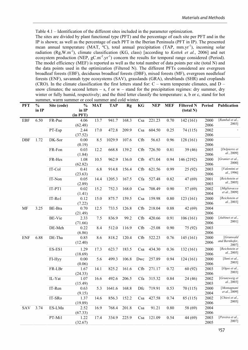
Materials and Methods
157
Table 4.1 – Identification of the different sites included in the parameter optimization. The sites are divided by plant functional type (PFT) and the percentage of each site per PFT and in the IP is shown; as well as the percentage of each PFT in the Iberian Peninsula (PFT in IP). The presented mean annual temperature (MAT, ºC), total annual precipitation (TAP, mm.yr-1), incoming solar radiation (Rg,W.m-2), climate classification (KG, class) [according to Kottek et al., 2006] and net ecosystem production (NEP, gC.m-2.yr-1) concern the results for temporal range considered (Period). The model efficiency (MEF) is reported as well as the total number of data points per site (total N) and the data points used in the optimization (Filtered N). The different PFTs considered are evergreen broadleaf forests (EBF), deciduous broadleaf forests (DBF), mixed forests (MF), evergreen needleleaf forests (ENF), savannah type ecosystems (SAV), grasslands (GRA), shrublands (SHR) and croplands (CRO). In the climate classification the first letters stand for: C – warm temperate climates, and D – snow climates; the second letters – s, f or w – stand for the precipitation regimes: dry summer, dry winter or fully humid, respectively; and the third letter classify the temperature: a, b or c, stand for hot summer, warm summer or cool summer and cold winter.
PFT % in IP
Site (code) % in IP
(in PFT)
MAT TAP Rg KG NEP MEF Filtered N (total N)
Period Publication
FR-Pue 4.06 (62.48)
13.7 941.7 168.3 Csa 221.23 0.70 142 (161) 20002006
[Rambal et al., 2003]
EBF 6.50
PT-Esp 2.44 (37.52)
17.0 472.8 209.9 Csa 604.50 0.25 74 (115) 20022006
-
DK-Sor 0.00 (0.19)
8.5 1029.9 107.6 Cfb 56.63 0.96 128 (161) 20002006
FR-Fon 0.03 (1.84)
12.2 668.8 139.2 Cfb 726.50 0.81 39 (46) 20052006
[Delpierre et al., 2009]
FR-Hes 1.08 (62.82)
10.5 962.9 136.0 Cfb 471.04 0.94 146 (2192) 20002006
[Granier et al., 2000]
IT-Col 0.41 (23.63)
6.8 914.8 156.4 Cfb 621.56 0.99 25 (92) 20032006
[Valentini et al., 1996]
IT-Non 0.05 (2.89)
14.4 1205.3 167.5 Cfa 527.48 0.82 47 (69) 20012003
[Reichstein et al., 2005]
IT-PT1 0.02 (1.41)
15.2 752.3 168.0 Csa 708.49 0.90 57 (69) 20022004
[Migliavacca et al., 2009]
DBF 1.72
IT-Ro1 0.12 (7.22)
15.0 875.7 159.5 Csa 159.98 0.80 123 (161) 20002006
[Reichstein et al., 2003]
BE-Bra 0.70 (21.49)
12.5 733.5 126.8 Cfb 218.04 0.88 42 (69) 20042006
BE-Vie 2.33 (71.66)
7.5 836.9 99.2 Cfb 420.66 0.91 106 (161) 20002006
[Aubinet et al., 2001]
MF 3.25
DE-Meh 0.22 (6.86)
8.4 512.0 116.9 Cfb -25.08 0.90 75 (92) 20032006
DE-Tha 0.85 (12.40)
8.6 818.2 120.4 Cfb 522.23 0.76 145 (161) 20002006
[Grunwald and Bernhofer,
2007]
ES-ES1 1.29 (18.69)
17.3 623.7 183.5 Csa 434.30 0.36 132 (161) 20002006
[Reichstein et al., 2005]
FI-Hyy 0.00 (0.06)
5.6 499.3 106.8 Dwc 257.89 0.94 124 (161) 20002006
[Suni et al., 2003]
FR-LBr 1.67 (24.33)
14.1 825.2 161.6 Cfb 271.17 0.72 60 (92) 20032006
[Ogee et al., 2003]
IL-Yat 1.07 (15.49)
16.6 492.6 206.5 Cfa 315.32 0.84 24 (46) 20022003
[Grunzweig et al., 2003]
IT-Ren 0.63 (9.15)
5.3 1641.6 168.8 Dfc 719.91 0.53 70 (115) 20002004
[Montagnani et al., 2009]
ENF 6.88
IT-SRo 1.37 (19.89)
14.6 856.3 152.2 Csa 427.58 0.74 85 (115) 20022006
[Chiesi et al., 2005]
ES-LMa 2.52 (67.33)
16.9 768.4 201.8 Csa 91.21 0.80 58 (69) 20042006
SAV 3.74
PT-Mi1 1.22 (32.67)
17.4 334.9 225.9 Csa 121.09 0.54 44 (69) 20032005
[Pereira et al., 2007]
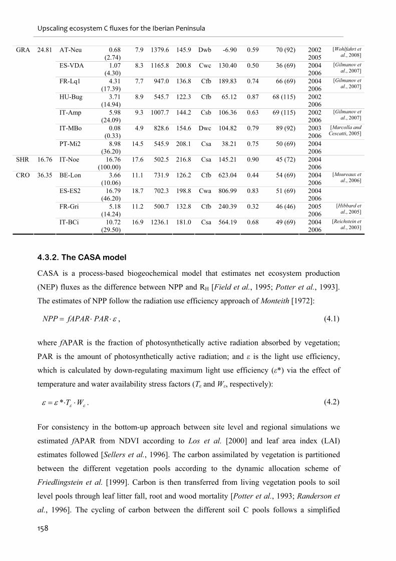
Upscaling ecosystem C fluxes for the Iberian Peninsula
158
AT-Neu 0.68(2.74)
7.9 1379.6 145.9 Dwb -6.90 0.59 70 (92) 2002 2005
[Wohlfahrt et al., 2008]
ES-VDA 1.07(4.30)
8.3 1165.8 200.8 Cwc 130.40 0.50 36 (69) 2004 2006
[Gilmanov et al., 2007]
FR-Lq1 4.31(17.39)
7.7 947.0 136.8 Cfb 189.83 0.74 66 (69) 2004 2006
[Gilmanov et al., 2007]
HU-Bug 3.71(14.94)
8.9 545.7 122.3 Cfb 65.12 0.87 68 (115) 2002 2006
IT-Amp 5.98(24.09)
9.3 1007.7 144.2 Csb 106.36 0.63 69 (115) 2002 2006
[Gilmanov et al., 2007]
IT-MBo 0.08(0.33)
4.9 828.6 154.6 Dwc 104.82 0.79 89 (92) 2003 2006
[Marcolla and Cescatti, 2005]
GRA 24.81
PT-Mi2 8.98(36.20)
14.5 545.9 208.1 Csa 38.21 0.75 50 (69) 2004 2006
SHR 16.76 IT-Noe 16.76(100.00)
17.6 502.5 216.8 Csa 145.21 0.90 45 (72) 2004 2006
BE-Lon 3.66(10.06)
11.1 731.9 126.2 Cfb 623.04 0.44 54 (69) 2004 2006
[Moureaux et al., 2006]
ES-ES2 16.79(46.20)
18.7 702.3 198.8 Cwa 806.99 0.83 51 (69) 2004 2006
FR-Gri 5.18(14.24)
11.2 500.7 132.8 Cfb 240.39 0.32 46 (46) 2005 2006
[Hibbard et al., 2005]
CRO 36.35
IT-BCi 10.72(29.50)
16.9 1236.1 181.0 Csa 564.19 0.68 49 (69) 2004 2006
[Reichstein et al., 2003]
4.3.2. The CASA model
CASA is a process-based biogeochemical model that estimates net ecosystem production
(NEP) fluxes as the difference between NPP and RH [Field et al., 1995; Potter et al., 1993].
The estimates of NPP follow the radiation use efficiency approach of Monteith [1972]:
PARfAPARNPP , (4.1)
where fAPAR is the fraction of photosynthetically active radiation absorbed by vegetation;
PAR is the amount of photosynthetically active radiation; and ε is the light use efficiency,
which is calculated by down-regulating maximum light use efficiency (ε*) via the effect of
temperature and water availability stress factors (Tε and Wε, respectively):
WT * . (4.2)
For consistency in the bottom-up approach between site level and regional simulations we
estimated fAPAR from NDVI according to Los et al. [2000] and leaf area index (LAI)
estimates followed [Sellers et al., 1996]. The carbon assimilated by vegetation is partitioned
between the different vegetation pools according to the dynamic allocation scheme of
Friedlingstein et al. [1999]. Carbon is then transferred from living vegetation pools to soil
level pools through leaf litter fall, root and wood mortality [Potter et al., 1993; Randerson et
al., 1996]. The cycling of carbon between the different soil C pools follows a simplified
Materials and Methods
159
version of the CENTURY model [Parton et al., 1987]. RH is estimated as the integral of
decomposition from the different soil C pools:
p
issiiH MTWkCR )1( ,
(4.3)
where each pool i is characterized by a different turnover rate ki that is regulated by the effect
of temperature (Ts) and water availability conditions (Ws) [Potter et al., 1993]. The carbon
content of each pool (Ci) results from the integrated transfers between the different pools,
which is further regulated by the carbon assimilation efficiency of microbes (Mε). In general,
the robustness of the CASA model has been corroborated by its wide application in studies
that range from ecosystem to global scales [e.g. Carvalhais et al., 2008; Randerson et al.,
2002] and focusing on different ecological and biogeochemical issues [e.g. Potter et al., 2001;
van der Werf et al., 2003].
4.3.3. Inverse model parameter optimization
The optimized parameters in the CASA model are responsible for governing the responses of
NPP and RH to environmental conditions (temperature and water availability) and maximum
energy mass conversion rates (maximum light use efficiency [Monteith, 1972]) [Potter et al.,
1993]. In addition, a parameter is introduced that adjusts the initial conditions of microbial
and more recalcitrant C pools after the spin-up routines – η – and regulates the ecosystem’s
initial distance to equilibrium [Carvalhais et al., 2008]. This relaxation of the steady-state
assumption gives a structural flexibility to the model that was shown to reduce parameter
uncertainties and biases from wrong structural model assumptions [Carvalhais et al., 2008].
Additional disequilibrium conditions can be observed in the vegetation pools which may
influence directly gross primary production and autotrophic respiration (RA) and indirectly
heterotrophic respiration fluxes (through transfer of carbon from vegetation to soil reservoirs)
[e.g. Nabuurs, 2004]. CASA relies on the implicit calculations of autotrophic respiration as a
fixed fraction of NPP, and estimates of NPP rely on inputs of fAPAR [Potter et al., 1993],
which minimizes the impacts of nonequilibrium conditions of vegetation on NPP. These
implicit considerations on RA do not decrement the CASA model’s ability to simulate net
ecosystem fluxes [Carvalhais et al., 2010, in press]. The model performance is also not
different between an exclusive consideration of nonequilibrium conditions in soil versus soil
and vegetation carbon pools, revealing η could compensate for the indirect effects of
nonequilibrium conditions in RH [Carvalhais et al., 2010, in press]. Given the amenability of
both representations and the straightforward treatment of η in the current exercise we opted by
Upscaling ecosystem C fluxes for the Iberian Peninsula
160
solely considering nonequilibrium in soil level carbon pools. The parameter optimization
method consisted of the minimization of the sum of residual squares between eddy-covariance
measurements and model estimates of biweekly NEP fluxes using the Levenberg-Marquardt
algorithm [Draper and Smith, 1981].
4.3.4. Upscaling of model parameters
The upscaling of model parameters aims at attributing parameter vectors optimized at site
level, on a per-pixel basis, to the whole Iberian Peninsula. The conceptual idea here is that,
within an ecosystem type or plant functional type (PFT), each pixel p in the map would be
treated according its similarity with eddy-covariance site j, and parameterized accordingly.
The assignment of a parameter vector to a given pixel p is supported by a nearest
neighbourhood classification of the climatic and phenological conditions: to a given pixel p,
the parameter vector S corresponding to site j (Sj) is attributed when the climate and
phenological characteristics of p are closer to j‘s than to any other site’s from the same PFT.
So, Sp=Sj when jpNjjp dd ,,...,1*
, minarg finds the minimum distances between climate and
phenological characteristics between a pixel p and an eddy-covariance site j calculated as
jpjp VVd ,NS1, . Here, Vp and Vj are vectors containing the normalized biweekly time
series of mean air temperature, precipitation and solar radiation for the period 1960 to1990;
and mean NDVI between 1982 and 2005. NS is the Nash-Sutcliffe coefficient:
N
ipip
N
iijip
jp
VV
VVVVNS
1
2
,
1
2,,
1, ,
(4.4)
which quantifies the relative association between two vectors over the association between the
reference vector and its mean (the nominal situation) [Janssen and Heuberger, 1995; Nash
and Sutcliffe, 1970], where N is the length of the vectors Vp and Vj (N = 96) and i the column
index of these vectors. In addition to providing a measure of association, the NS also
measures the agreement between two vectors (proximity to the 1:1 line). Consequently, the
climatic-phenological distance measure (from here on identified as CPd) reflects both the
proximity in the magnitude and seasonality of climate and phenology drivers between site
level observations and the regional datasets for the IP. The results associate one site of each
PFT per pixel which means that if a given PFT is present in that pixel the respective parameter
vector corresponds to the site where the climate and phenological characteristics are closer to
the pixel’s.
Materials and Methods
161
4.3.5. Data for spatial runs
Due to the diagnostic nature of CASA, the temporal extent of the model runs for the Iberian
Peninsula was bounded by the longest remotely sensed NDVI record available: the Global
Inventory Modelling and Mapping Studies (GIMMS) NDVI [Tucker et al., 2005]. The option
of using the biweekly MODIS NDVI products (2 by 2 window of 250m x 250m pixels) for
site level evaluation of the model and the GIMMS NDVI datasets (8km x 8km pixels) for the
regional runs was based on two assumptions: 1) the eddy-covariance footprint depends on the
local conditions [Gockede et al., 2008] and height of the tower [Barcza et al., 2009] but
generally is not larger than 1km2, making the 8km by 8km areas too large for representation of
the eddy-covariance data; and 2) the MODIS and GIMMS NDVI products are comparable
[Tucker et al., 2005].
Monthly climate datasets – air temperature, precipitation and solar radiation – at 10’ spatial
resolution since 1901 until 2000 are available from the Climate Research Unit of the
University of East Anglia [Mitchell et al., 2004]. The climate datasets were extended until
2006 using pixel level empirical relationships with coarser climate datasets. For temperature
and solar radiation we made use of 0.25 degrees datasets from the Global Land Data
Assimilation System [Rodell et al., 2004]. Precipitation was extended using 0.5 degrees
datasets from the University of Delaware [Matsuura and Willmott, 2007]. Every dataset was
spatially interpolated to the GIMMS NDVI 8km by 8km grid following Zhao et al. [2005].
We used linear interpolation to downscale from monthly to biweekly periods.
The soil properties – texture fractions and soil depth – were extracted from the Soil Map of
the European Communities [The Commission of the European Communities, 1985]. The
proportion of each PFT within every 8km by 8km pixel is defined by the CORINE land cover
map [Bossard et al., 2000] The fraction of forest PFTs is defined by the tree cover value of
the MODIS vegetation continuous fields at 1km [Hansen et al., 2003] bounded by the class
intervals defined in each CORINE class.
4.3.6. Regional model runs for a range of initial conditions
The CASA model estimates of ecosystem fluxes for the Iberian Peninsula are performed on a
PFT basis: the parameter vector used per pixel per PFT originates from the upscaling exercise
above. The ecosystem fluxes per pixel p (e.g. NEPp) are estimated by integrating all the
individual PFT estimates (e.g. NEPp,PFT) weighted by the fraction of each PFT inside that
pixel p (fPFTp):
Upscaling ecosystem C fluxes for the Iberian Peninsula
162
PFTp
n
PFTpp NEPfPFTNEP ,
1
, (4.5)
For each PFT the model is always spun-up with a mean yearly dataset until steady state after
which a range of nonequilibrium conditions is forced on the more recalcitrant and microbial
soil carbon pools. The prescription of different distances to equilibrium is obtained by
multiplying these pools by the scalar η after the spin-up and then running the model forward.
We create a range of initial conditions, from significant sinks (η << 1) to sources (η >> 1) by
changing the η values between 0.01 and 2 (in 0.1 increments). The ensemble of runs obtained
allows evaluating the impacts of different distances to equilibrium in the inter-annual
variability and temporal trends in net ecosystem fluxes.
4.3.7. Decoupling the drivers effects on ecosystem fluxes from the initial
conditions
It is recognized that the steady-state estimates of the soil carbon pools are a function of the
model parameterization and environmental drivers prescribed for the spin-up [Andrén and
Kätterer, 1997]. Hence, for the same model parameterization and drivers, any prescribed
distance of the soil C pools to equilibrium (η) yields a dynamic recovery response towards
equilibrium with the simulation drivers. The recovery from a prescribed η can yield conditions
different from the steady state as a response to the simulation’s climate and/or phenology time
series. It is essential to distinguish or isolate the effects of the drivers from the recovery
dynamics on the ecosystem fluxes. Here, we opted for removing the recovery dynamics by
performing parallel model runs with constant drivers. In these runs the climate and phenology
drivers were identical to the spin-up runs datasets: the mean year of the complete 25 year time
series. Further, we prescribed the exact same parameterization and η scalars used in the
regular forward model runs. To obtain a climate-phenology, not recovery, driven NEP time
series (NEPD, Table 4.2) we subtracted the fluxes estimated with the constant drivers (NEPK,
Table 4.2) from the NEP time series:
KD NEPNEPNEP . (4.6)
With this procedure we can remove the variance and trajectories of NEP resulting from the
soil C pools recovery and investigate the responses of fluxes to the climate and phenological
drivers.
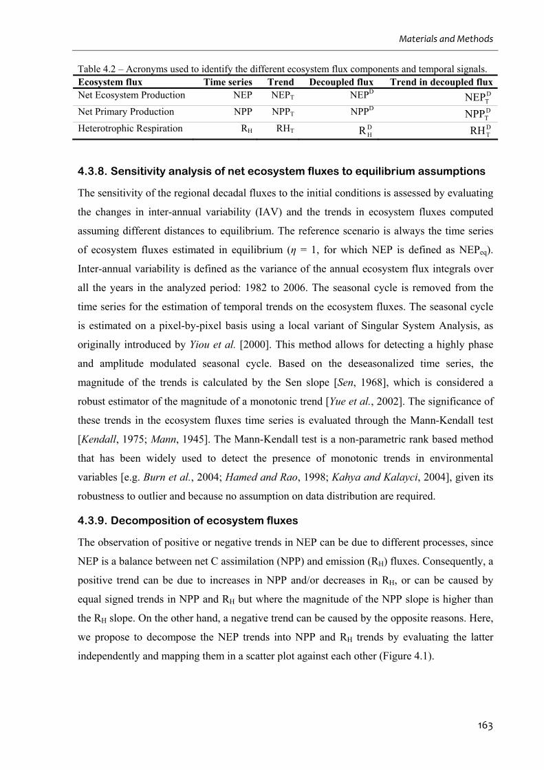
Materials and Methods
163
Table 4.2 – Acronyms used to identify the different ecosystem flux components and temporal signals. Ecosystem flux Time series Trend Decoupled flux Trend in decoupled fluxNet Ecosystem Production NEP NEPT NEPD D
TNEPNet Primary Production NPP NPPT NPPD D
TNPPHeterotrophic Respiration RH RHT
DHR D
TRH
4.3.8. Sensitivity analysis of net ecosystem fluxes to equilibrium assumptions
The sensitivity of the regional decadal fluxes to the initial conditions is assessed by evaluating
the changes in inter-annual variability (IAV) and the trends in ecosystem fluxes computed
assuming different distances to equilibrium. The reference scenario is always the time series
of ecosystem fluxes estimated in equilibrium (η = 1, for which NEP is defined as NEPeq).
Inter-annual variability is defined as the variance of the annual ecosystem flux integrals over
all the years in the analyzed period: 1982 to 2006. The seasonal cycle is removed from the
time series for the estimation of temporal trends on the ecosystem fluxes. The seasonal cycle
is estimated on a pixel-by-pixel basis using a local variant of Singular System Analysis, as
originally introduced by Yiou et al. [2000]. This method allows for detecting a highly phase
and amplitude modulated seasonal cycle. Based on the deseasonalized time series, the
magnitude of the trends is calculated by the Sen slope [Sen, 1968], which is considered a
robust estimator of the magnitude of a monotonic trend [Yue et al., 2002]. The significance of
these trends in the ecosystem fluxes time series is evaluated through the Mann-Kendall test
[Kendall, 1975; Mann, 1945]. The Mann-Kendall test is a non-parametric rank based method
that has been widely used to detect the presence of monotonic trends in environmental
variables [e.g. Burn et al., 2004; Hamed and Rao, 1998; Kahya and Kalayci, 2004], given its
robustness to outlier and because no assumption on data distribution are required.
4.3.9. Decomposition of ecosystem fluxes
The observation of positive or negative trends in NEP can be due to different processes, since
NEP is a balance between net C assimilation (NPP) and emission (RH) fluxes. Consequently, a
positive trend can be due to increases in NPP and/or decreases in RH, or can be caused by
equal signed trends in NPP and RH but where the magnitude of the NPP slope is higher than
the RH slope. On the other hand, a negative trend can be caused by the opposite reasons. Here,
we propose to decompose the NEP trends into NPP and RH trends by evaluating the latter
independently and mapping them in a scatter plot against each other (Figure 4.1).
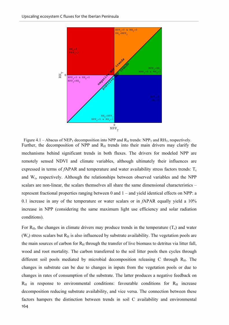
Upscaling ecosystem C fluxes for the Iberian Peninsula
164
0
0
NPPT
RHT
negative NEP trends
positive NEP trends
RHT>0
NPPT<0
NPPT>0
RHT<0
NPPT<0 & RH
T<0
NPPT<RH
T
RHT<NPP
TNPP
T<0 & RH
T<0
NPPT>0 & RH
T>0
RHT>NPP
T
NPPT>RH
TNPP
T>0 & RH
T>0
Figure 4.1 – Abacus of NEPT decomposition into NPP and RH trends: NPPT and RHT, respectively. Further, the decomposition of NPP and RH trends into their main drivers may clarify the
mechanisms behind significant trends in both fluxes. The drivers for modeled NPP are
remotely sensed NDVI and climate variables, although ultimately their influences are
expressed in terms of fAPAR and temperature and water availability stress factors trends: Tε
and Wε, respectively. Although the relationships between observed variables and the NPP
scalars are non-linear, the scalars themselves all share the same dimensional characteristics –
represent fractional properties ranging between 0 and 1 – and yield identical effects on NPP: a
0.1 increase in any of the temperature or water scalars or in fAPAR equally yield a 10%
increase in NPP (considering the same maximum light use efficiency and solar radiation
conditions).
For RH, the changes in climate drivers may produce trends in the temperature (Ts) and water
(Ws) stress scalars but RH is also influenced by substrate availability. The vegetation pools are
the main sources of carbon for RH through the transfer of live biomass to detritus via litter fall,
wood and root mortality. The carbon transferred to the soil litter pools then cycles through
different soil pools mediated by microbial decomposition releasing C through RH. The
changes in substrate can be due to changes in inputs from the vegetation pools or due to
changes in rates of consumption of the substrate. The latter produces a negative feedback on
RH in response to environmental conditions: favourable conditions for RH increase
decomposition reducing substrate availability, and vice versa. The connection between these
factors hampers the distinction between trends in soil C availability and environmental
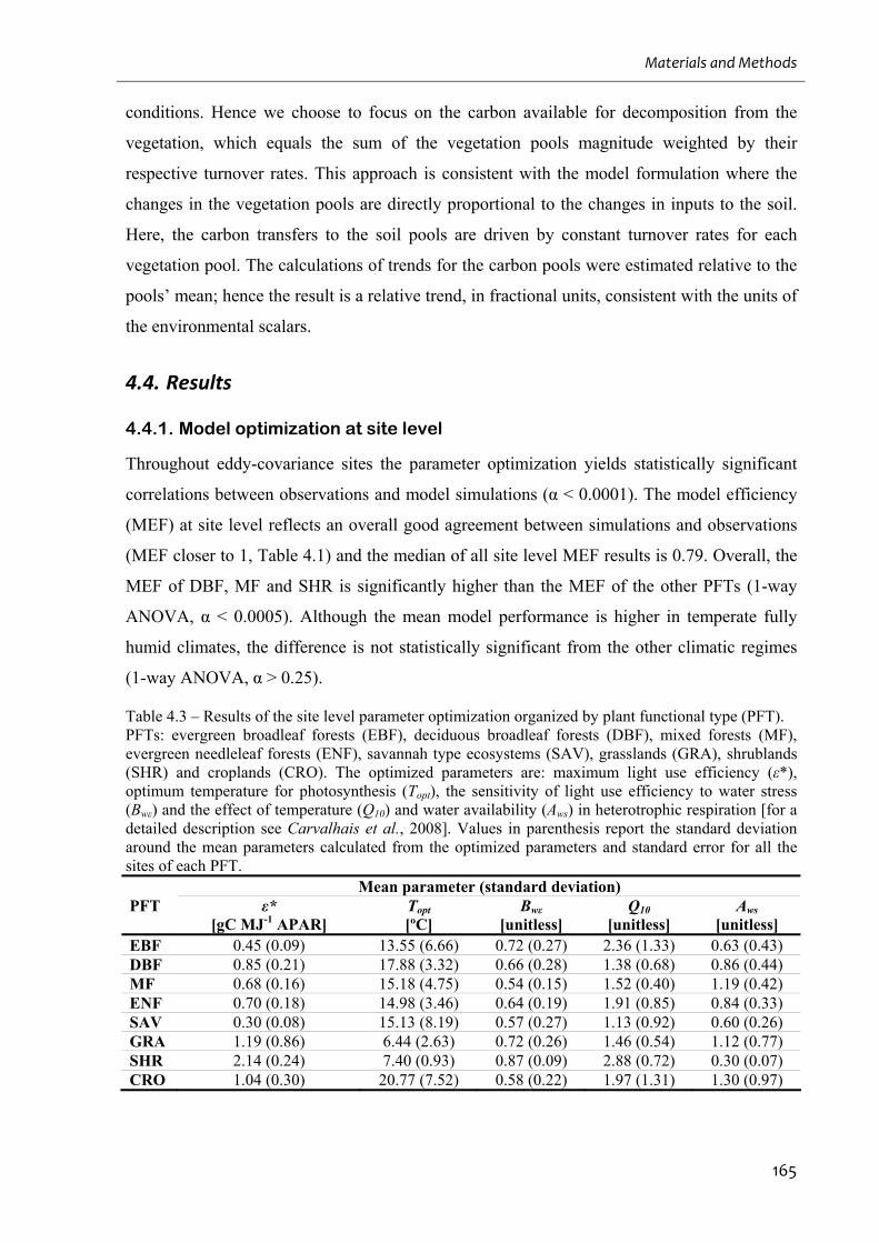
Materials and Methods
165
conditions. Hence we choose to focus on the carbon available for decomposition from the
vegetation, which equals the sum of the vegetation pools magnitude weighted by their
respective turnover rates. This approach is consistent with the model formulation where the
changes in the vegetation pools are directly proportional to the changes in inputs to the soil.
Here, the carbon transfers to the soil pools are driven by constant turnover rates for each
vegetation pool. The calculations of trends for the carbon pools were estimated relative to the
pools’ mean; hence the result is a relative trend, in fractional units, consistent with the units of
the environmental scalars.
4.4. Results
4.4.1. Model optimization at site level
Throughout eddy-covariance sites the parameter optimization yields statistically significant
correlations between observations and model simulations (α < 0.0001). The model efficiency
(MEF) at site level reflects an overall good agreement between simulations and observations
(MEF closer to 1, Table 4.1) and the median of all site level MEF results is 0.79. Overall, the
MEF of DBF, MF and SHR is significantly higher than the MEF of the other PFTs (1-way
ANOVA, α < 0.0005). Although the mean model performance is higher in temperate fully
humid climates, the difference is not statistically significant from the other climatic regimes
(1-way ANOVA, α > 0.25).
Table 4.3 – Results of the site level parameter optimization organized by plant functional type (PFT). PFTs: evergreen broadleaf forests (EBF), deciduous broadleaf forests (DBF), mixed forests (MF), evergreen needleleaf forests (ENF), savannah type ecosystems (SAV), grasslands (GRA), shrublands (SHR) and croplands (CRO). The optimized parameters are: maximum light use efficiency (ε*), optimum temperature for photosynthesis (Topt), the sensitivity of light use efficiency to water stress (Bwε) and the effect of temperature (Q10) and water availability (Aws) in heterotrophic respiration [for a detailed description see Carvalhais et al., 2008]. Values in parenthesis report the standard deviation around the mean parameters calculated from the optimized parameters and standard error for all the sites of each PFT. Mean parameter (standard deviation) PFT ε*
[gC MJ-1 APAR] Topt [ºC]
Bwε [unitless]
Q10 [unitless]
Aws [unitless]
EBF 0.45 (0.09) 13.55 (6.66) 0.72 (0.27) 2.36 (1.33) 0.63 (0.43) DBF 0.85 (0.21) 17.88 (3.32) 0.66 (0.28) 1.38 (0.68) 0.86 (0.44) MF 0.68 (0.16) 15.18 (4.75) 0.54 (0.15) 1.52 (0.40) 1.19 (0.42) ENF 0.70 (0.18) 14.98 (3.46) 0.64 (0.19) 1.91 (0.85) 0.84 (0.33) SAV 0.30 (0.08) 15.13 (8.19) 0.57 (0.27) 1.13 (0.92) 0.60 (0.26) GRA 1.19 (0.86) 6.44 (2.63) 0.72 (0.26) 1.46 (0.54) 1.12 (0.77) SHR 2.14 (0.24) 7.40 (0.93) 0.87 (0.09) 2.88 (0.72) 0.30 (0.07) CRO 1.04 (0.30) 20.77 (7.52) 0.58 (0.22) 1.97 (1.31) 1.30 (0.97)
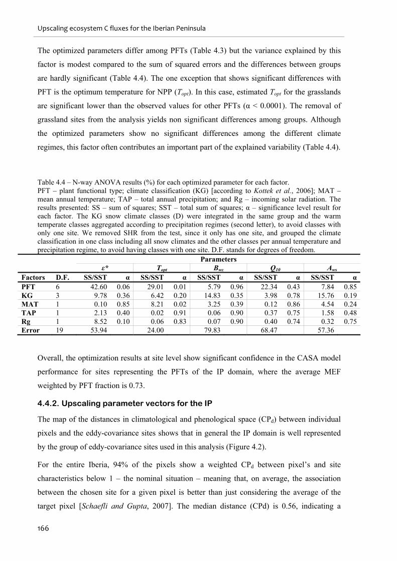
Upscaling ecosystem C fluxes for the Iberian Peninsula
166
The optimized parameters differ among PFTs (Table 4.3) but the variance explained by this
factor is modest compared to the sum of squared errors and the differences between groups
are hardly significant (Table 4.4). The one exception that shows significant differences with
PFT is the optimum temperature for NPP (Topt). In this case, estimated Topt for the grasslands
are significant lower than the observed values for other PFTs (α < 0.0001). The removal of
grassland sites from the analysis yields non significant differences among groups. Although
the optimized parameters show no significant differences among the different climate
regimes, this factor often contributes an important part of the explained variability (Table 4.4).
Table 4.4 – N-way ANOVA results (%) for each optimized parameter for each factor. PFT – plant functional type; climate classification (KG) [according to Kottek et al., 2006]; MAT – mean annual temperature; TAP – total annual precipitation; and Rg – incoming solar radiation. The results presented: SS – sum of squares; SST – total sum of squares; α – significance level result for each factor. The KG snow climate classes (D) were integrated in the same group and the warm temperate classes aggregated according to precipitation regimes (second letter), to avoid classes with only one site. We removed SHR from the test, since it only has one site, and grouped the climate classification in one class including all snow climates and the other classes per annual temperature and precipitation regime, to avoid having classes with one site. D.F. stands for degrees of freedom.
Parameters ε* Topt Bwε Q10 Aws Factors D.F. SS/SST α SS/SST α SS/SST α SS/SST α SS/SST αPFT 6 42.60 0.06 29.01 0.01 5.79 0.96 22.34 0.43 7.84 0.85KG 3 9.78 0.36 6.42 0.20 14.83 0.35 3.98 0.78 15.76 0.19MAT 1 0.10 0.85 8.21 0.02 3.25 0.39 0.12 0.86 4.54 0.24TAP 1 2.13 0.40 0.02 0.91 0.06 0.90 0.37 0.75 1.58 0.48Rg 1 8.52 0.10 0.06 0.83 0.07 0.90 0.40 0.74 0.32 0.75Error 19 53.94 24.00 79.83 68.47 57.36
Overall, the optimization results at site level show significant confidence in the CASA model
performance for sites representing the PFTs of the IP domain, where the average MEF
weighted by PFT fraction is 0.73.
4.4.2. Upscaling parameter vectors for the IP
The map of the distances in climatological and phenological space (CPd) between individual
pixels and the eddy-covariance sites shows that in general the IP domain is well represented
by the group of eddy-covariance sites used in this analysis (Figure 4.2).
For the entire Iberia, 94% of the pixels show a weighted CPd between pixel’s and site
characteristics below 1 – the nominal situation – meaning that, on average, the association
between the chosen site for a given pixel is better than just considering the average of the
target pixel [Schaefli and Gupta, 2007]. The median distance (CPd) is 0.56, indicating a
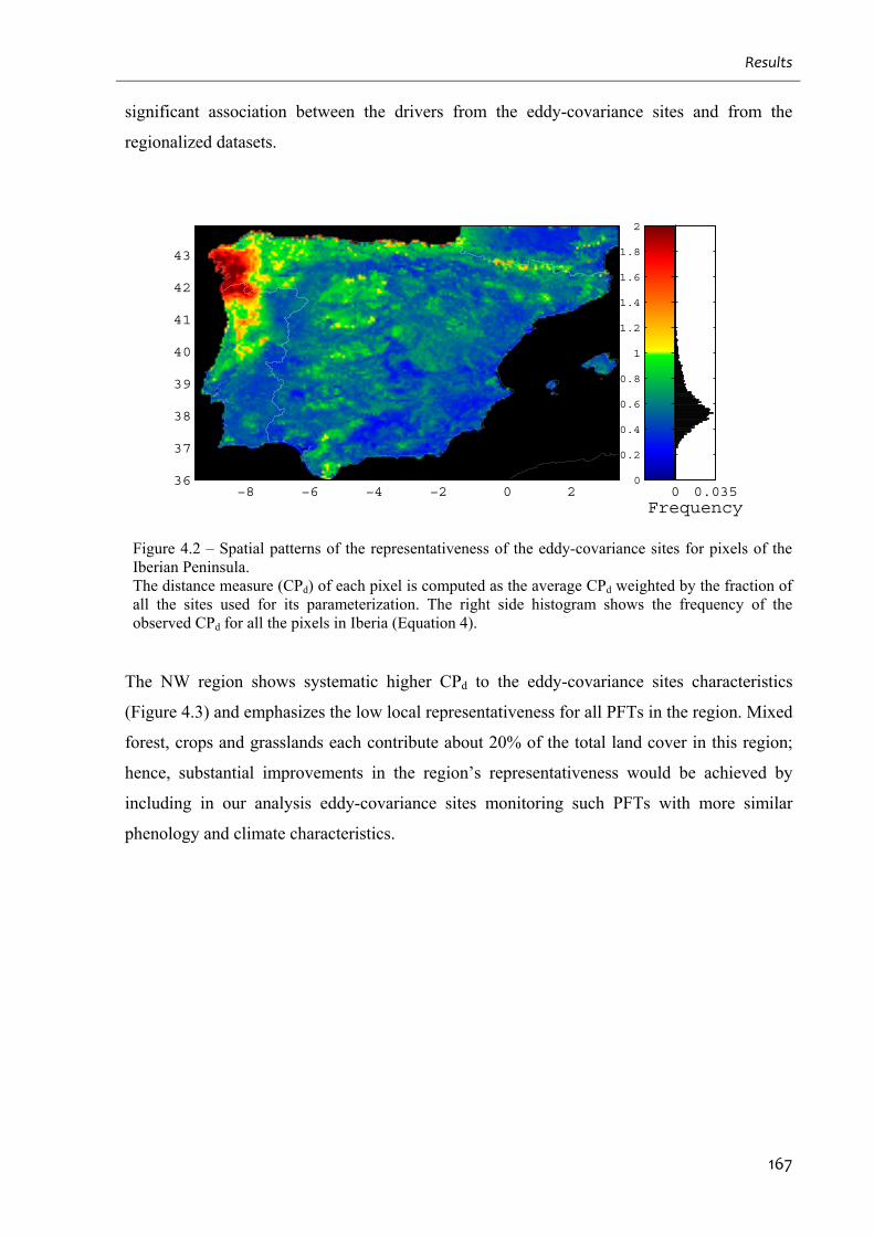
Results
167
significant association between the drivers from the eddy-covariance sites and from the
regionalized datasets.
−8 −6 −4 −2 0 236
37
38
39
40
41
42
43
0
0.2
0.4
0.6
0.8
1
1.2
1.4
1.6
1.8
2
0 0.035Frequency
Figure 4.2 – Spatial patterns of the representativeness of the eddy-covariance sites for pixels of the Iberian Peninsula. The distance measure (CPd) of each pixel is computed as the average CPd weighted by the fraction of all the sites used for its parameterization. The right side histogram shows the frequency of the observed CPd for all the pixels in Iberia (Equation 4).
The NW region shows systematic higher CPd to the eddy-covariance sites characteristics
(Figure 4.3) and emphasizes the low local representativeness for all PFTs in the region. Mixed
forest, crops and grasslands each contribute about 20% of the total land cover in this region;
hence, substantial improvements in the region’s representativeness would be achieved by
including in our analysis eddy-covariance sites monitoring such PFTs with more similar
phenology and climate characteristics.
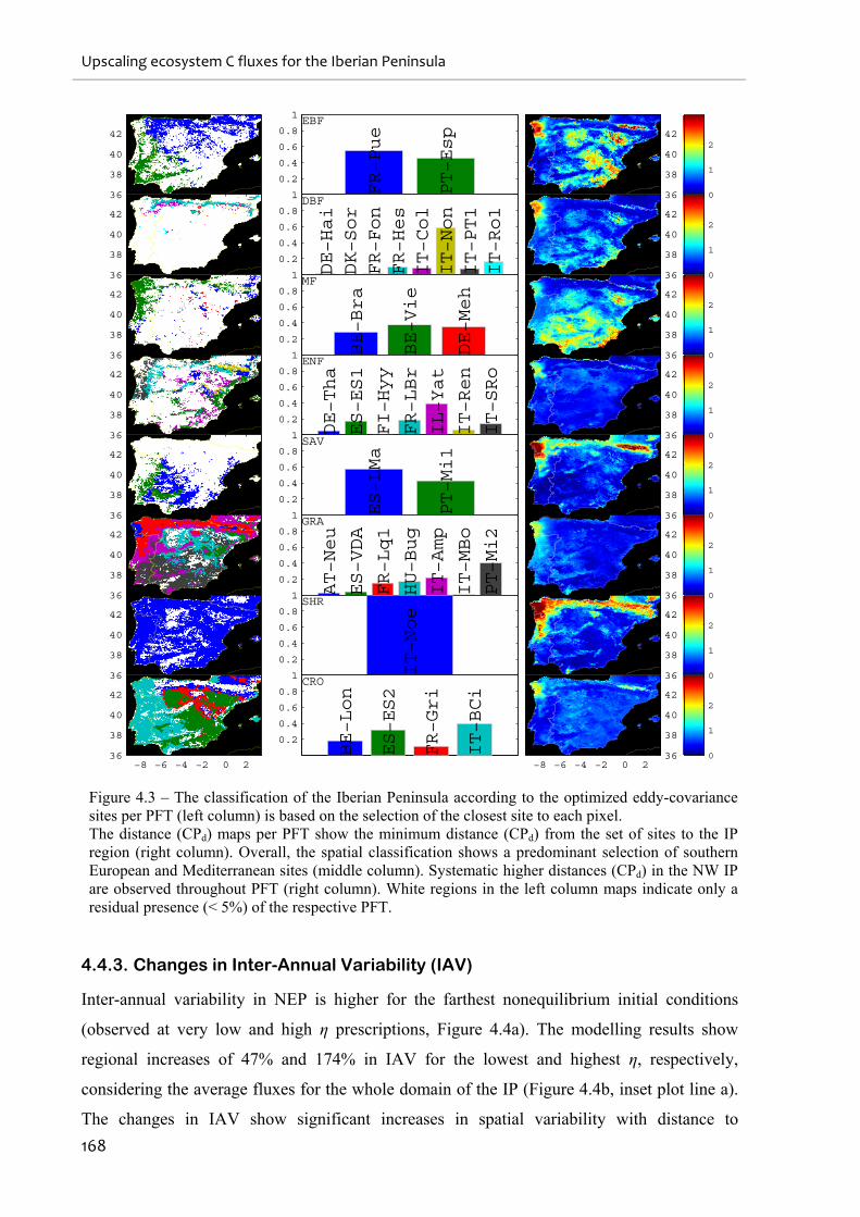
Upscaling ecosystem C fluxes for the Iberian Peninsula
168
−8 −6 −4 −2 0 236
38
40
42
0.2
0.4
0.6
0.8
1
FR−Pue
PT−Esp
EBF
−8 −6 −4 −2 0 236
38
40
42
0
1
2
−8 −6 −4 −2 0 236
38
40
42
0.2
0.4
0.6
0.8
1
DE−Hai
DK−Sor
FR−Fon
FR−Hes
IT−Col
IT−Non
IT−PT1
IT−Ro1
DBF
−8 −6 −4 −2 0 236
38
40
42
0
1
2
−8 −6 −4 −2 0 236
38
40
42
0.2
0.4
0.6
0.8
1
BE−Bra
BE−Vie
DE−Meh
MF
−8 −6 −4 −2 0 236
38
40
42
0
1
2
−8 −6 −4 −2 0 236
38
40
42
0.2
0.4
0.6
0.8
1
DE−Tha
ES−ES1
FI−Hyy
FR−LBr
IL−Yat
IT−Ren
IT−SRo
ENF
−8 −6 −4 −2 0 236
38
40
42
0
1
2
−8 −6 −4 −2 0 236
38
40
42
0.2
0.4
0.6
0.8
1
ES−LMa
PT−Mi1
SAV
−8 −6 −4 −2 0 236
38
40
42
0
1
2
−8 −6 −4 −2 0 236
38
40
42
0.2
0.4
0.6
0.8
1
AT−Neu
ES−VDA
FR−Lq1
HU−Bug
IT−Amp
IT−MBo
PT−Mi2
GRA
−8 −6 −4 −2 0 236
38
40
42
0
1
2
−8 −6 −4 −2 0 236
38
40
42
0.2
0.4
0.6
0.8
1
IT−Noe
SHR
−8 −6 −4 −2 0 236
38
40
42
0
1
2
−8 −6 −4 −2 0 236
38
40
42
0.2
0.4
0.6
0.8
1
BE−Lon
ES−ES2
FR−Gri
IT−BCi
CRO
−8 −6 −4 −2 0 236
38
40
42
0
1
2
Figure 4.3 – The classification of the Iberian Peninsula according to the optimized eddy-covariance sites per PFT (left column) is based on the selection of the closest site to each pixel. The distance (CPd) maps per PFT show the minimum distance (CPd) from the set of sites to the IP region (right column). Overall, the spatial classification shows a predominant selection of southern European and Mediterranean sites (middle column). Systematic higher distances (CPd) in the NW IP are observed throughout PFT (right column). White regions in the left column maps indicate only a residual presence (< 5%) of the respective PFT.
4.4.3. Changes in Inter-Annual Variability (IAV)
Inter-annual variability in NEP is higher for the farthest nonequilibrium initial conditions
(observed at very low and high η prescriptions, Figure 4.4a). The modelling results show
regional increases of 47% and 174% in IAV for the lowest and highest η, respectively,
considering the average fluxes for the whole domain of the IP (Figure 4.4b, inset plot line a).
The changes in IAV show significant increases in spatial variability with distance to
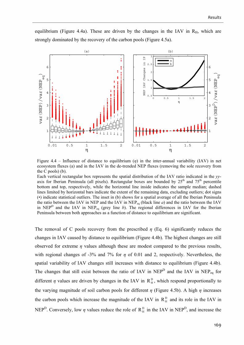
Results
169
equilibrium (Figure 4.4a). These are driven by the changes in the IAV in RH, which are
strongly dominated by the recovery of the carbon pools (Figure 4.5a).
0.01 0.5 1 1.5 2
1
2
3
4
5
6
var(NEP)/var(NEPeq)
η
(a)
0.01 0.5 1 1.5 2
1
2
3
4
5
6
var(NEPD)/var(NEPeq)
η
(b)
0 0.5 1 1.5 20.5
1
1.5
2
2.5
3
η
NEP IAV Changes in IP
ab
Figure 4.4 – Influence of distance to equilibrium (η) in the inter-annual variability (IAV) in net ecosystem fluxes (a) and in the IAV in the de-trended NEP fluxes (removing the sole recovery from the C pools) (b). Each vertical rectangular box represents the spatial distribution of the IAV ratio indicated in the yy-axis for Iberian Peninsula (all pixels). Rectangular boxes are bounded by 25th and 75th percentile bottom and top, respectively, while the horizontal line inside indicates the sample median; dashed lines limited by horizontal bars indicate the extent of the remaining data, excluding outliers; dot signs (•) indicate statistical outliers. The inset in (b) shows for a spatial average of all the Iberian Peninsula the ratio between the IAV in NEP and the IAV in NEPeq (black line a) and the ratio between the IAV in NEPD and the IAV in NEPeq (grey line b). The regional differences in IAV for the Iberian Peninsula between both approaches as a function of distance to equilibrium are significant.
The removal of C pools recovery from the prescribed η (Eq. 6) significantly reduces the
changes in IAV caused by distance to equilibrium (Figure 4.4b). The highest changes are still
observed for extreme η values although these are modest compared to the previous results,
with regional changes of -3% and 7% for η of 0.01 and 2, respectively. Nevertheless, the
spatial variability of IAV changes still increases with distance to equilibrium (Figure 4.4b).
The changes that still exist between the ratio of IAV in NEPD and the IAV in NEPeq for
different η values are driven by changes in the IAV in DHR , which respond proportionally to
the varying magnitude of soil carbon pools for different η (Figure 4.5b). A high η increases
the carbon pools which increase the magnitude of the IAV in DHR and its role in the IAV in
NEPD. Conversely, low η values reduce the role of DHR in the IAV in NEPD, and increase the
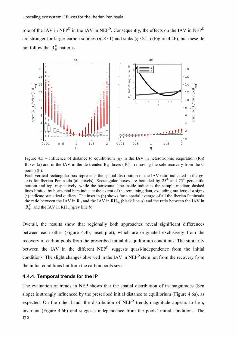
Upscaling ecosystem C fluxes for the Iberian Peninsula
170
role of the IAV in NPPD in the IAV in NEPD. Consequently, the effects on the IAV in NEPD
are stronger for larger carbon sources (η >> 1) and sinks (η << 1) (Figure 4.4b), but these do
not follow the DHR patterns.
0.01 0.5 1 1.5 2
0
2
4
6
8
10
12
14
16
18
var(RH)/var(RHeq)
η
(a)
0.01 0.5 1 1.5 2
0
2
4
6
8
10
12
14
16
18
var(RHD)/var(RHeq)
η
(b)
0 0.5 1 1.5 20
1
2
3
4
5
6
η
RH IAV Changes in IP
ab
Figure 4.5 – Influence of distance to equilibrium (η) in the IAV in heterotrophic respiration (RH)
fluxes (a) and in the IAV in the de-trended RH fluxes ( DHR , removing the sole recovery from the C
pools) (b). Each vertical rectangular box represents the spatial distribution of the IAV ratio indicated in the yy-axis for Iberian Peninsula (all pixels). Rectangular boxes are bounded by 25th and 75th percentile bottom and top, respectively, while the horizontal line inside indicates the sample median; dashed lines limited by horizontal bars indicate the extent of the remaining data, excluding outliers; dot signs (•) indicate statistical outliers. The inset in (b) shows for a spatial average of all the Iberian Peninsula the ratio between the IAV in RH and the IAV in RHeq (black line a) and the ratio between the IAV in
DHR and the IAV in RHeq (grey line b).
Overall, the results show that regionally both approaches reveal significant differences
between each other (Figure 4.4b, inset plot), which are originated exclusively from the
recovery of carbon pools from the prescribed initial disequilibrium conditions. The similarity
between the IAV in the different NEPD suggests quasi-independence from the initial
conditions. The slight changes observed in the IAV in NEPD stem not from the recovery from
the initial conditions but from the carbon pools sizes.
4.4.4. Temporal trends for the IP
The evaluation of trends in NEP shows that the spatial distribution of its magnitudes (Sen
slope) is strongly influenced by the prescribed initial distance to equilibrium (Figure 4.6a), as
expected. On the other hand, the distribution of NEPD trends magnitude appears to be η
invariant (Figure 4.6b) and suggests independence from the pools’ initial conditions. The
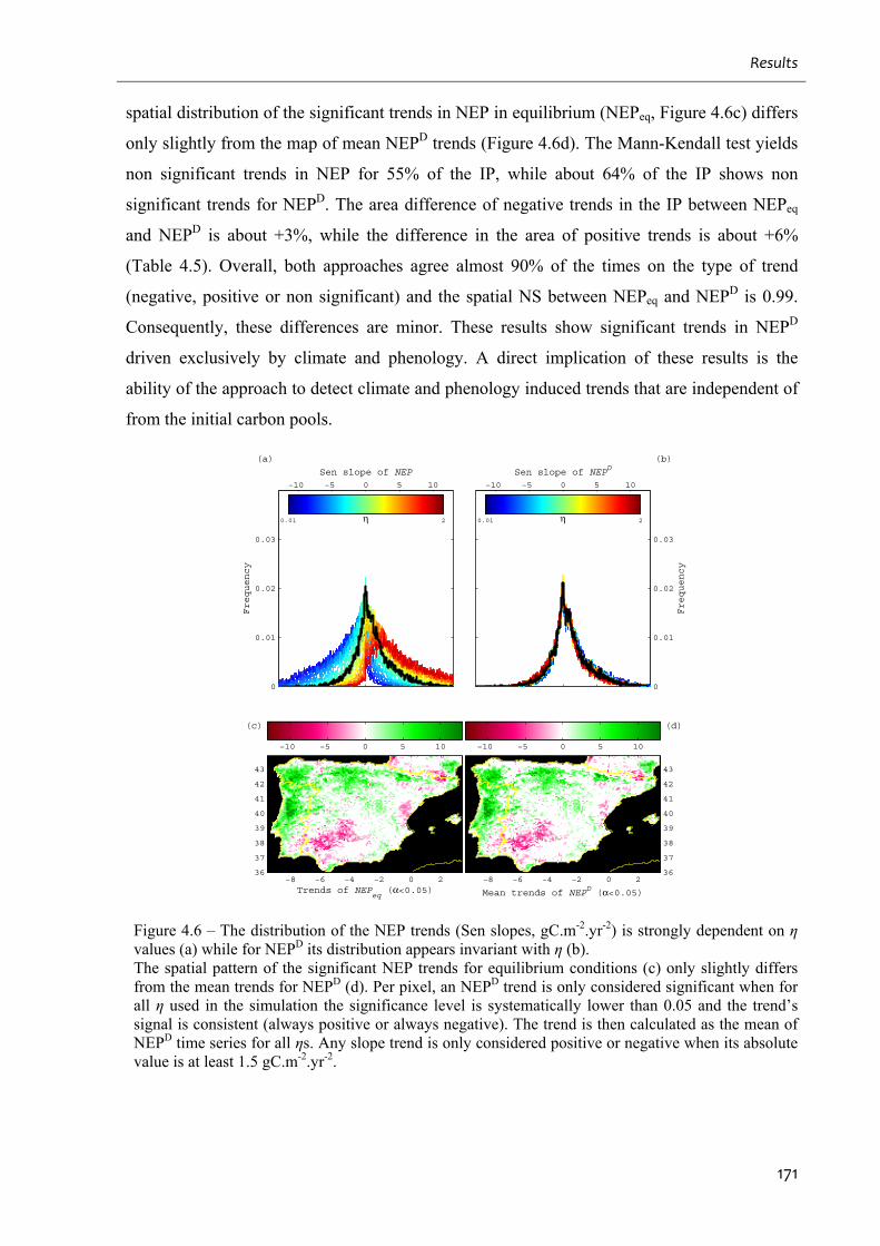
Results
171
spatial distribution of the significant trends in NEP in equilibrium (NEPeq, Figure 4.6c) differs
only slightly from the map of mean NEPD trends (Figure 4.6d). The Mann-Kendall test yields
non significant trends in NEP for 55% of the IP, while about 64% of the IP shows non
significant trends for NEPD. The area difference of negative trends in the IP between NEPeq
and NEPD is about +3%, while the difference in the area of positive trends is about +6%
(Table 4.5). Overall, both approaches agree almost 90% of the times on the type of trend
(negative, positive or non significant) and the spatial NS between NEPeq and NEPD is 0.99.
Consequently, these differences are minor. These results show significant trends in NEPD
driven exclusively by climate and phenology. A direct implication of these results is the
ability of the approach to detect climate and phenology induced trends that are independent of
from the initial carbon pools.
Trends of NEPeq (α<0.05)
−8 −6 −4 −2 0 236
37
38
39
40
41
42
43
−10 −5 0 5 10
−10 −5 0 5 10
0
0.01
0.02
0.03
Sen slope of NEP
Frequency
η0.01 2
Mean trends of NEPD (α<0.05)
−8 −6 −4 −2 0 236
37
38
39
40
41
42
43
−10 −5 0 5 10
−10 −5 0 5 10
0
0.01
0.02
0.03
Sen slope of NEPD
Frequency
η0.01 2
(c)
(a)
(d)
(b)
Figure 4.6 – The distribution of the NEP trends (Sen slopes, gC.m-2.yr-2) is strongly dependent on η values (a) while for NEPD its distribution appears invariant with η (b). The spatial pattern of the significant NEP trends for equilibrium conditions (c) only slightly differs from the mean trends for NEPD (d). Per pixel, an NEPD trend is only considered significant when for all η used in the simulation the significance level is systematically lower than 0.05 and the trend’s signal is consistent (always positive or always negative). The trend is then calculated as the mean of NEPD time series for all ηs. Any slope trend is only considered positive or negative when its absolute value is at least 1.5 gC.m-2.yr-2.
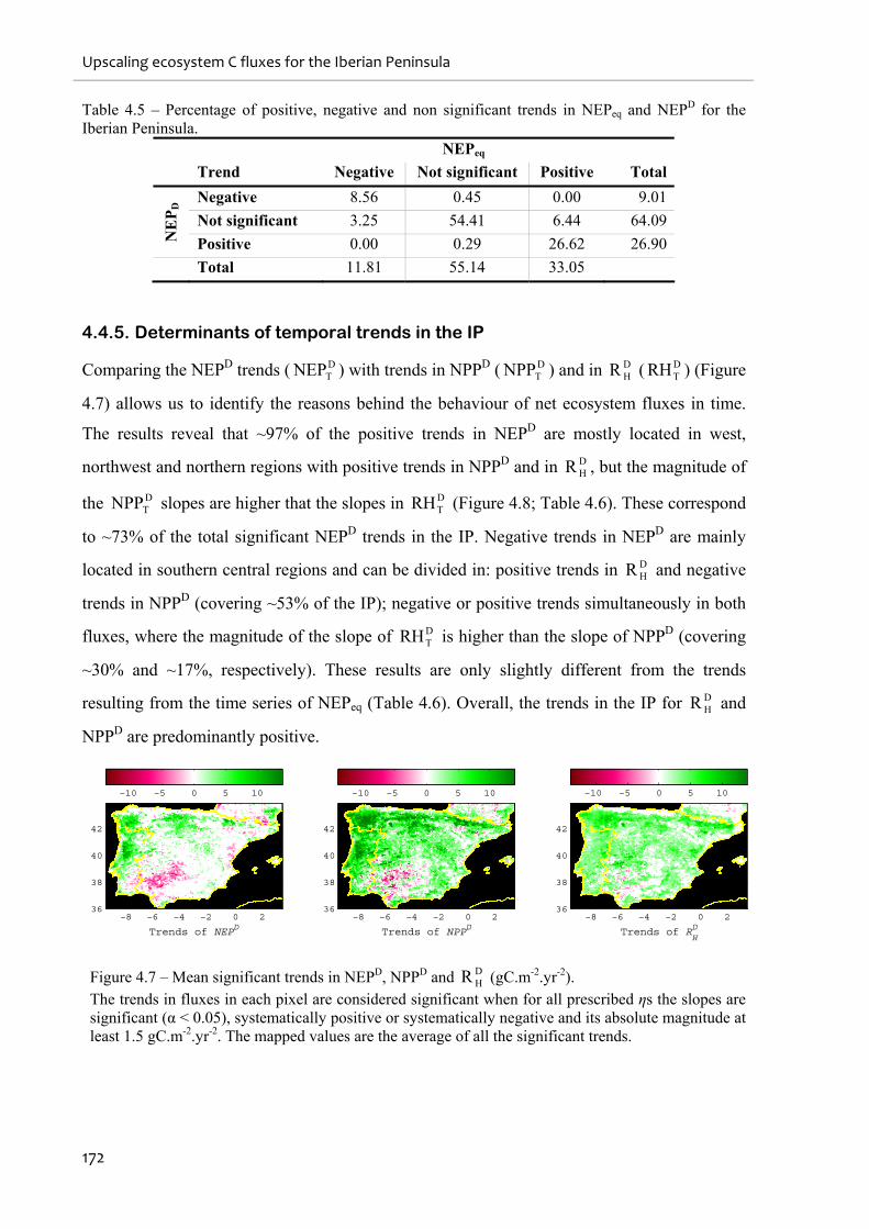
Upscaling ecosystem C fluxes for the Iberian Peninsula
172
Table 4.5 – Percentage of positive, negative and non significant trends in NEPeq and NEPD for the Iberian Peninsula.
NEPeq
Trend Negative Not significant Positive Total
Negative 8.56 0.45 0.00 9.01
Not significant 3.25 54.41 6.44 64.09
NE
PD
Positive 0.00 0.29 26.62 26.90
Total 11.81 55.14 33.05
4.4.5. Determinants of temporal trends in the IP
Comparing the NEPD trends ( DTNEP ) with trends in NPPD ( D
TNPP ) and in DHR ( D
TRH ) (Figure
4.7) allows us to identify the reasons behind the behaviour of net ecosystem fluxes in time.
The results reveal that ~97% of the positive trends in NEPD are mostly located in west,
northwest and northern regions with positive trends in NPPD and in DHR , but the magnitude of
the DTNPP slopes are higher that the slopes in D
TRH (Figure 4.8; Table 4.6). These correspond
to ~73% of the total significant NEPD trends in the IP. Negative trends in NEPD are mainly
located in southern central regions and can be divided in: positive trends in DHR and negative
trends in NPPD (covering ~53% of the IP); negative or positive trends simultaneously in both
fluxes, where the magnitude of the slope of DTRH is higher than the slope of NPPD (covering
~30% and ~17%, respectively). These results are only slightly different from the trends
resulting from the time series of NEPeq (Table 4.6). Overall, the trends in the IP for DHR and
NPPD are predominantly positive.
Trends of NEPD
−8 −6 −4 −2 0 236
38
40
42
−10 −5 0 5 10
Trends of NPPD
−8 −6 −4 −2 0 236
38
40
42
−10 −5 0 5 10
Trends of RHD
−8 −6 −4 −2 0 236
38
40
42
−10 −5 0 5 10
Figure 4.7 – Mean significant trends in NEPD, NPPD and DHR (gC.m-2.yr-2).
The trends in fluxes in each pixel are considered significant when for all prescribed ηs the slopes are significant (α < 0.05), systematically positive or systematically negative and its absolute magnitude at least 1.5 gC.m-2.yr-2. The mapped values are the average of all the significant trends.
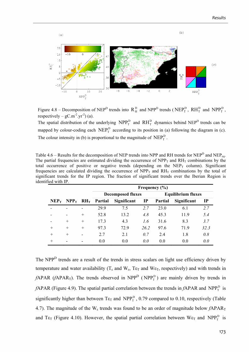
Results
173
Figure 4.8 – Decomposition of NEPD trends into DHR and NPPD trends ( D
TNEP , DTRH and D
TNPP , respectively – gC.m-2.yr-2) (a).
The spatial distribution of the underlying DTNPP and D
TRH dynamics behind NEPD trends can be
mapped by colour-coding each DTNEP according to its position in (a) following the diagram in (c).
The colour intensity in (b) is proportional to the magnitude of DTNEP .
Table 4.6 – Results for the decomposition of NEP trends into NPP and RH trends for NEPD and NEPeq. The partial frequencies are estimated dividing the occurrence of NPPT and RHT combinations by the total occurrence of positive or negative trends (depending on the NEPT column). Significant frequencies are calculated dividing the occurrence of NPPT and RHT combinations by the total of significant trends for the IP region. The fraction of significant trends over the Iberian Region is identified with IP.
Frequency (%) Decomposed fluxes Equilibrium fluxes
NEPT NPPT RHT Partial Significant IP Partial Significant IP
- - - 29.9 7.5 2.7 23.0 6.1 2.7
- - + 52.8 13.2 4.8 45.3 11.9 5.4
- + + 17.3 4.3 1.6 31.6 8.3 3.7
+ + + 97.3 72.9 26.2 97.6 71.9 32.3
+ + - 2.7 2.1 0.7 2.4 1.8 0.8
+ - - 0.0 0.0 0.0 0.0 0.0 0.0
The NPPD trends are a result of the trends in stress scalars on light use efficiency driven by
temperature and water availability (Tε and Wε, TεT and WεT, respectively) and with trends in
fAPAR (fAPART). The trends observed in NPPD ( DTNPP ) are mainly driven by trends in
fAPAR (Figure 4.9). The spatial partial correlation between the trends in fAPAR and DTNPP is
significantly higher than between TεT and DTNPP , 0.79 compared to 0.10, respectively (Table
4.7). The magnitude of the Wε trends was found to be an order of magnitude below fAPART
and TεT (Figure 4.10). However, the spatial partial correlation between WεT and DTNPP is
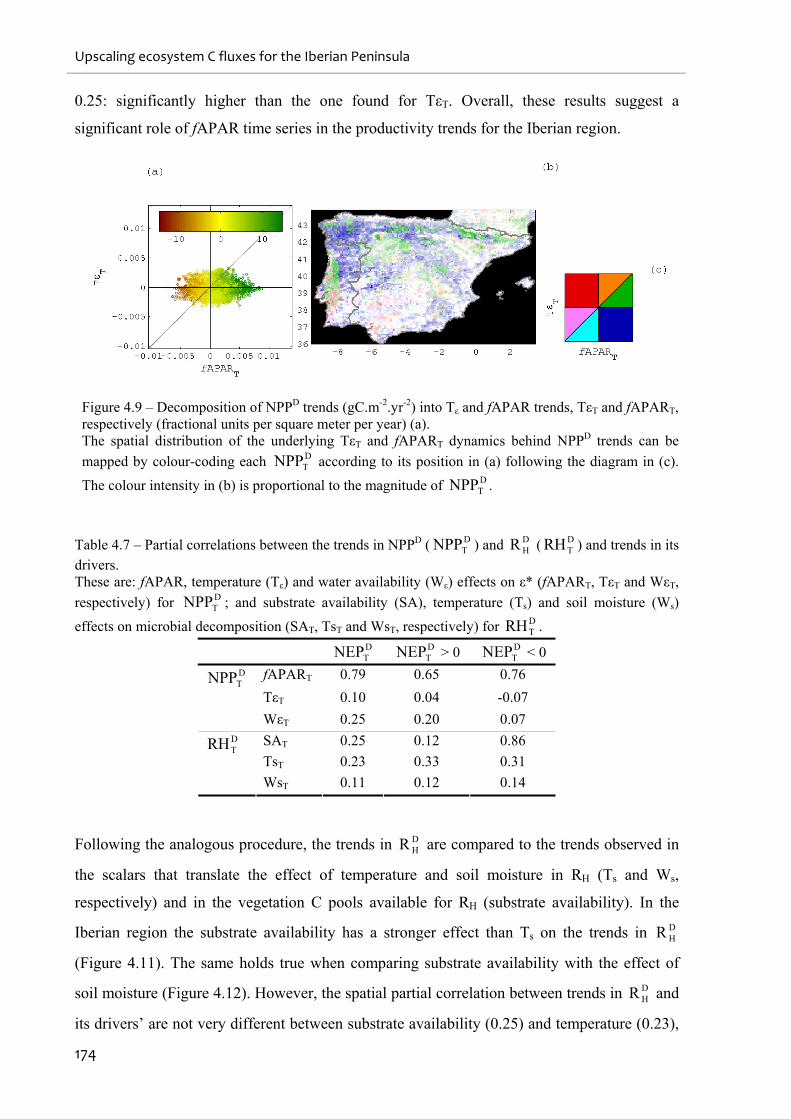
Upscaling ecosystem C fluxes for the Iberian Peninsula
174
0.25: significantly higher than the one found for TεT. Overall, these results suggest a
significant role of fAPAR time series in the productivity trends for the Iberian region.
Figure 4.9 – Decomposition of NPPD trends (gC.m-2.yr-2) into Tε and fAPAR trends, TεT and fAPART, respectively (fractional units per square meter per year) (a). The spatial distribution of the underlying TεT and fAPART dynamics behind NPPD trends can be
mapped by colour-coding each DTNPP according to its position in (a) following the diagram in (c).
The colour intensity in (b) is proportional to the magnitude of DTNPP .
Table 4.7 – Partial correlations between the trends in NPPD ( DTNPP ) and D
HR ( DTRH ) and trends in its
drivers. These are: fAPAR, temperature (Tε) and water availability (Wε) effects on ε* (fAPART, TεT and WεT,
respectively) for DTNPP ; and substrate availability (SA), temperature (Ts) and soil moisture (Ws)
effects on microbial decomposition (SAT, TsT and WsT, respectively) for DTRH .
DTNEP D
TNEP > 0 DTNEP < 0
fAPART 0.79 0.65 0.76
TεT 0.10 0.04 -0.07
DTNPP
WεT 0.25 0.20 0.07
SAT 0.25 0.12 0.86
TsT 0.23 0.33 0.31
DTRH
WsT 0.11 0.12 0.14
Following the analogous procedure, the trends in DHR are compared to the trends observed in
the scalars that translate the effect of temperature and soil moisture in RH (Ts and Ws,
respectively) and in the vegetation C pools available for RH (substrate availability). In the
Iberian region the substrate availability has a stronger effect than Ts on the trends in DHR
(Figure 4.11). The same holds true when comparing substrate availability with the effect of
soil moisture (Figure 4.12). However, the spatial partial correlation between trends in DHR and
its drivers’ are not very different between substrate availability (0.25) and temperature (0.23),
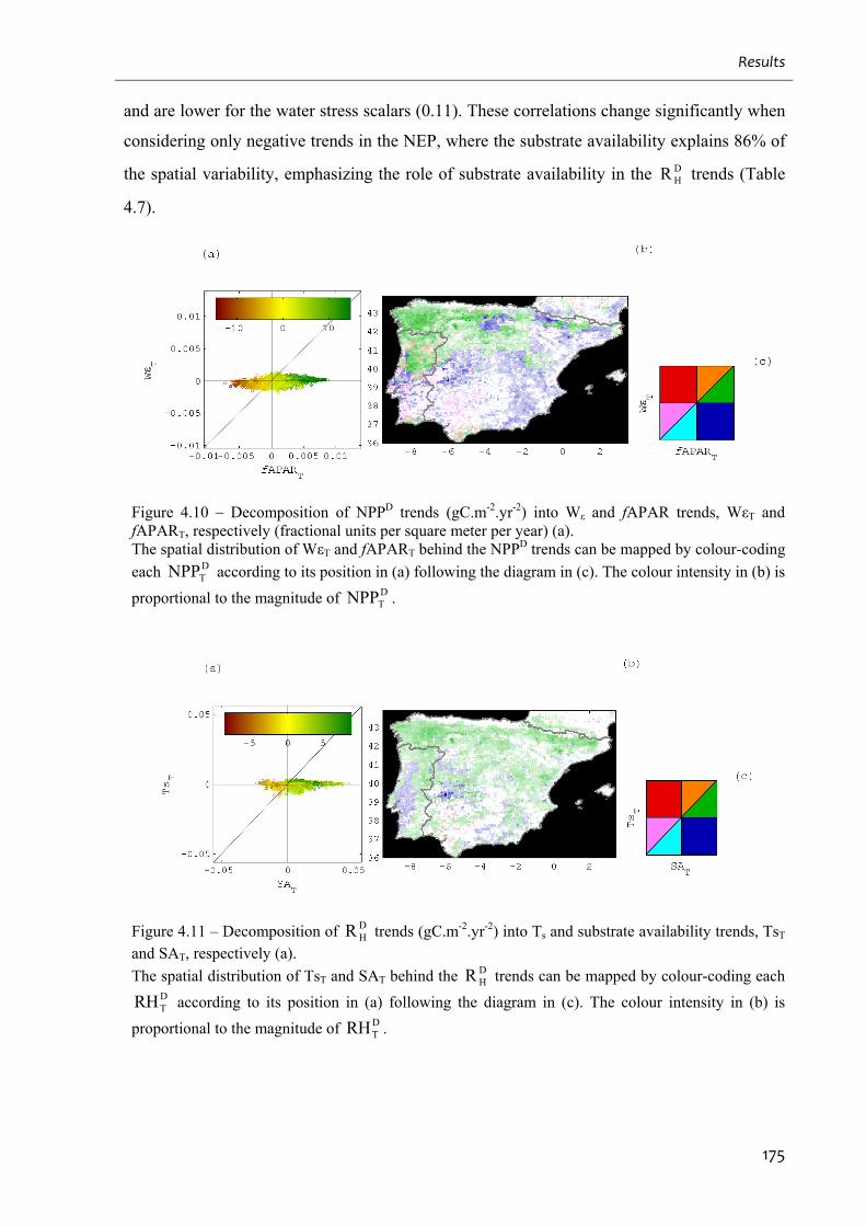
Results
175
and are lower for the water stress scalars (0.11). These correlations change significantly when
considering only negative trends in the NEP, where the substrate availability explains 86% of
the spatial variability, emphasizing the role of substrate availability in the DHR trends (Table
4.7).
Figure 4.10 – Decomposition of NPPD trends (gC.m-2.yr-2) into Wε and fAPAR trends, WεT and fAPART, respectively (fractional units per square meter per year) (a). The spatial distribution of WεT and fAPART behind the NPPD trends can be mapped by colour-coding
each DTNPP according to its position in (a) following the diagram in (c). The colour intensity in (b) is
proportional to the magnitude of DTNPP .
Figure 4.11 – Decomposition of DHR trends (gC.m-2.yr-2) into Ts and substrate availability trends, TsT
and SAT, respectively (a).
The spatial distribution of TsT and SAT behind the DHR trends can be mapped by colour-coding each
DTRH according to its position in (a) following the diagram in (c). The colour intensity in (b) is
proportional to the magnitude of DTRH .
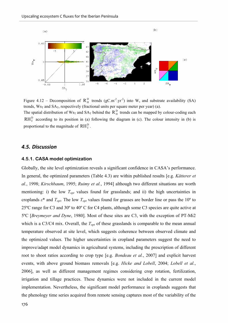
Upscaling ecosystem C fluxes for the Iberian Peninsula
176
Figure 4.12 – Decomposition of DHR trends (gC.m-2.yr-2) into Ws and substrate availability (SA)
trends, WsT and SAT, respectively (fractional units per square meter per year) (a).
The spatial distribution of WsT and SAT behind the DHR trends can be mapped by colour-coding each
DTRH according to its position in (a) following the diagram in (c). The colour intensity in (b) is
proportional to the magnitude of DTRH .
4.5. Discussion
4.5.1. CASA model optimization
Globally, the site level optimization reveals a significant confidence in CASA’s performance.
In general, the optimized parameters (Table 4.3) are within published results [e.g. Kätterer et
al., 1998; Kirschbaum, 1995; Ruimy et al., 1994] although two different situations are worth
mentioning: i) the low Topt values found for grasslands; and ii) the high uncertainties in
croplands ε* and Topt. The low Topt values found for grasses are border line or pass the 10º to
25ºC range for C3 and 30º to 40º C for C4 plants, although some C3 species are quite active at
5ºC [Breymeyer and Dyne, 1980]. Most of these sites are C3, with the exception of PT-Mi2
which is a C3/C4 mix. Overall, the Topt of these grasslands is comparable to the mean annual
temperature observed at site level, which suggests coherence between observed climate and
the optimized values. The higher uncertainties in cropland parameters suggest the need to
improve/adapt model dynamics in agricultural systems, including the prescription of different
root to shoot ratios according to crop type [e.g. Bondeau et al., 2007] and explicit harvest
events, with above ground biomass removals [e.g. Hicke and Lobell, 2004; Lobell et al.,
2006], as well as different management regimes considering crop rotation, fertilization,
irrigation and tillage practices. These dynamics were not included in the current model
implementation. Nevertheless, the significant model performance in croplands suggests that
the phenology time series acquired from remote sensing captures most of the variability of the
Discussion
177
NPP. Further, in site level optimizations, the lack of harvest removal of C from the leaf pools
that then feeds the soil pools can be approximated by reductions in η. For the purpose of this
study, the absence of such dynamics in model simulations is unlikely to change our results.
4.5.2. Upscaling parameter vectors for the IP
The results reveal systematic lower representativeness in the North-western IP region which is
generally identified as a high productivity area in regional and global studies [e.g. Jung et al.,
2008]. Representativeness in this region is low for all PFTs (Figure 4.3), which reveals that
the under-representation is related to the phenological and climate variables used in the
classification. Improved representativeness in this region will require more flux measurements
from mixed forests, crops or grassland sites with similar bioclimatic characteristics. Further,
only one observational site was available representing shrub lands for the entire IP.
The current approach identifies the limitations in the sample of eddy-covariance sites for
representing the regional ecosystems in the IP. Similar approaches would be useful in
assisting network design or for selection of possible site locations in future network updates.
Certainly these are dependent on the goals of the monitoring and modelling exercises. Here,
the main factors explaining the variability of parameters are often the plant function type and
the climate regime observed at site level (Table 4.4). These results lend support to the
conceptual approach taken here to upscale the CASA model parameters. However, there is
still a significant fraction of unexplained variability in the parameters and our bottom-up
approach does not address issues related to the variability of parameters within the same PFT
or climate regime. Increasing the number of sites and including other factors in the analysis –
such as disturbance or management regimes – are two important issues to consider towards
more comprehensive upscaling and modelling exercises. In this regard we recognize the
importance of prescribing management [e.g. Bondeau et al., 2007] or disturbance [e.g. van der
Werf et al., 2003] regimes, as well as the effects of nutrients dynamics [e.g. Zaehle et al.,
2010].
4.5.3. Dynamics of ecosystem fluxes induced by climate and phenology
The effects of different initial conditions on the IAV and temporal trends in NEP were higher
for the highest departures from equilibrium, as expected. Since the spin-up routines were
performed with an average climate and phenology dataset, the modeled recovery from the
initial perturbations (η) is expected to lead to similar ecosystem states (carbon pools). The
farthest positive departures from equilibrium (NEP >> 0 since η << 1) create an initial sink
condition that is then attenuated and consequently leads to the steepest negative slopes of NEP
Upscaling ecosystem C fluxes for the Iberian Peninsula
178
trends. In these cases, carbon is accumulated in the soil pools with time, enhancing RH
through increases in substrate availability, and therefore decrementing NEP in time.
Oppositely, the farthest negative departures from equilibrium (NEP << 0 since η >> 1) force
an initial carbon source by increasing the soil pools. The increase in substrate availability
boosts RH in the beginning of the simulation which is reduced in time, generating a positive
trend in NEP. Consequently, the highest changes in the IAV in NEP are observed when
extreme departures from steady state are prescribed.
The extraction of the carbon pools dynamics (NEPK) from the NEP time series allows
exploring the impact of non steady-state conditions in the purely climate and phenology
driven dynamics of NEP (NEPD). The significant reduction in IAV changes (Figure 4.4) and
the distribution of the NEP trends with η (Figure 4.6a) emphasize the role of the carbon pools
dynamics in the estimation of ecosystem fluxes. These results show that simulated net
ecosystem fluxes can strongly diverge depending on initial conditions assumptions.
Additionally, the trends in the NEPD time series show a strong insensitivity to η revealing
independence from the initial estimates of C pools (Figure 4.6b). The results exhibit the
potential of NEPD to isolate and diagnose climate and phenology driven trends in ecosystem
fluxes. By identifying significant and consistent trends in NEPD we’re able to map regions of
robust trends in the Iberian region.
The differences between the spatial distribution of trends in NEPD and NEPeq are minor and
reveal that here the climate and phenology driven dynamics are quasi-independent from the
initial steady-state conditions (Figure 4.6c, d). Using a mean yearly dataset of drivers during
the period 1982-2006 ensures the adjustment of carbon pools to the mean of the drivers of the
run. The adjustments follow first order dynamics that are intrinsic to the model structure
(CASA's and many other biogeochemical models). This means that we can isolate the effects
of unknown initial conditions by removing NEPK to the NEP results. The result is the retrieval
of a time series of NEPD that is quasi-independent from the initial conditions of carbon pools.
In the current experiments these independent trends are analogous to the trends in NEPeq
because the dataset that drives NEPK is equal to the spin-up dataset. Consequently, as an
alternative to spinning-up the models until equilibrium this approach advocates advantages to
explore the effects of drivers in net ecosystem fluxes independently of the initial conditions of
pools.
We should add that ultimately the overall absolute NEP trends are not independent from the
initial conditions. Although removing carbon pools dynamics from the ecosystem fluxes may
allow independence from equilibrium assumptions, such procedure does not solve the initial
Discussion
179
state problem and our ability to quantify temporal trends is still limited. Beside model
structure the estimated fluxes depend not only on the model drivers – climate and
phenological drivers – but also on the parameters estimated at site level. In this regard, the
exhaustive accounting of terrestrial C fluxes implies the explicit integration of disturbances
and management regimes that were not simulated – especially agriculture and fire – for the
estimation of net biome production [Chapin et al., 2006]. In addition, the extension of the
current exercise to living pools in nonequilibrium conditions can be aided by prospective
remotely sensed estimations of above ground biomass.
4.5.4. Decomposition of ecosystem fluxes
The comparison between NEPD trends and the trends in its component fluxes, NPPD and DHR ,
discloses the dynamics behind the positive and negative trends in NEPD. For most of the
Iberian region the positive trends in NEPD are associated with positive trends in NPPD and in
DHR , although the slopes magnitudes are higher for NPPD. These results are consistent with
recent modelling studies [Piao et al., 2009a] and with eddy-covariance based studies that
advocate the significant role of gross primary production in driving NEP [e.g. Baldocchi,
2008; Reichstein et al., 2007]. The positive trends in NPPD are more strongly linked to
positive trends in fAPAR than to the climate effects on light use efficiency. Since fAPAR
estimates are based on the NDVI datasets, the modeled positive NPP trends are mostly driven
by phenological data rather then climate data. The fAPAR time series are estimated from
NDVI [following Los et al., 2000], hence the trends results demonstrate the role of NDVI
time series in driving the trends in NPP [cf. Jung et al., 2008].
The close association between climate and vegetation implies that the NDVI signal itself
embodies effects of climate regimes and patterns in the phenological characteristics of the
vegetation [e.g. Myneni et al., 1997]. In the CASA model the temperature stress scalars are
conceptually associated to adjustments in autotrophic respiration costs while the water stress
on canopy productivity can be ascribed to reductions in stomatal conductance [Potter et al.,
1993]. However, the plants’ response mechanisms to environmental stress can yield impacts
in APAR, ε or both. In this regard, current studies have highlighted the limitations of using
NDVI or fAPAR to detect instantaneous light use efficiency changes as a function of water
and temperature stress [e.g. Goerner et al., 2009; Grace et al., 2007]. It is then implicit in the
model structure that the environmental effects on ε and on fAPAR are complimentary for the
estimation of NPP and act at different time scales. Hence, here, only the effects of temperature
Upscaling ecosystem C fluxes for the Iberian Peninsula
180
and water availability on light used efficiency can be decomposed from the primary
productivity signal.
The main mechanism behind positive trends in the net ecosystem fluxes originates from
increases in primary production (mostly driven by fAPAR) that consequently increase the
vegetation carbon pools and the substrate availability for heterotrophic respiration. Here, the
absolute role of substrate availability is in general significantly higher than the effects of
temperature or soil moisture on the trends in DHR .
In areas of negative NEPD trends the partial correlation between the spatial patterns of trends
in DHR and substrate availability is significantly higher (Table 4.7). In these cases ( D
TNEP <0)
the increments in substrate availability are not attributable to increases in NPP, since most of
the trends in fAPAR (89%) as well as in NPPD (83%) are negative. Here, when DTRH >0, the
positive trends in substrate availability (75%) are mainly associated to positive trends in the
root pools (88%). These positive trends in the root pools are contrary to the trends observed in
NPPD. This apparent contrary behaviour results from increases in the carbon allocated to the
below ground vegetation pools caused by negative trends in the water stress scalars of ε*
(88%), increasing water stress. The investment in the root pools is associated with the
increasing trends in water stresses and is consistent with the dynamic allocation scheme by
Friedlingstein et al. [1999]. Due to the higher turnover rates of the fine root pools – compared
to the wood pools – the changes in the allocation strategies increase the availability of carbon
for decomposition. These observations highlight that the contribution of climate for long term
changes in heterotrophic respiration cannot be dissociated from the availability of material for
decomposition [Trumbore and Czimczik, 2008].
4.6. Conclusions
Our bottom-up approach allowed us to investigate the influences of the initial conditions in
modelling regional net ecosystem fluxes. Overall, the site level optimization results showed
significant confidence in model performance. Additionally, the set of sites selected are, in
general, significant representative of the Iberian Peninsula. Our approach also highlights
locations of systematic poorer representation ability: the North-western region, suggesting a
strong need to expand monitoring in this area. Consequently, the CASA model reveals itself
as a robust diagnostic approach to estimate NEP fluxes and the methodology to upscale
parameter vectors allows the identification of less represented regions. The presented bottom-
Conclusions
181
up approach emphasizes the relevance of analogous methods for the design of ecosystem
monitoring networks.
The influence of the initial conditions on NEP trends and inter-annual variability is
significant, as expected. However, we present a method to distinguish between the model
intrinsic dynamics following initialization routines and the fluxes variability only induced by
the drivers. Consequently, we are able to investigate the inter-annual variability and trends in
fluxes quasi-independently from the initial conditions. The relevance of such approach
emerges from the fact that most of the time the initial conditions of regional or global
simulations are unknown.
The results for the Iberian Peninsula show that the trends in the net ecosystem fluxes are
strongly linked to trends in primary production. The positive trends in the net ecosystem
fluxes are observed in western and northern regions with positive trends in both primary
production and heterotrophic respiration fluxes. Here, the magnitudes of the trends are higher
for the primary production fluxes. These are generally driven by positive trends in fAPAR,
that drive positive trends in NPPD, vegetation pools and consequently in the substrate
availability for decomposition at the soil level. Further, in regions of negative trends in net
ecosystem fluxes located mainly in Southern IP, the positive trends in heterotrophic
respiration are associated to positive trends in temperature as well as in substrate availability.
The positive trends in substrate availability result from changes in carbon allocation strategies
that are driven by positive trends in water stress. Overall, these modelling results suggest a
strong link between the component processes of net ecosystem fluxes. Further, the significant
role of fAPAR in NPPD trends and of substrate availability in DHR trends emphasizes that the
underlying mechanisms of trends in net ecosystem fluxes are strongly – but not necessarily
linearly – associated with primary production and allocation.
Overall, our results show that isolating the time series of ecosystem fluxes from the initial
conditions allows the identification of the effects of drivers on fluxes’ trends, which suggest
significant advantages for the estimation of the sensitivity of ecosystem fluxes to climate
drivers. The alleviation of the initialization uncertainty is significantly relevant to long term
modelling studies of net ecosystem fluxes.
Acknowledgements
We would like to thank Nicolas Delpierre, Ivan Janssens and Leonardo Montagnani for useful
comments on the manuscript and Jim Tucker, Ed Pak and Jorge Pinzon for the GIMMS NDVI
Upscaling ecosystem C fluxes for the Iberian Peninsula
182
datasets, as well as to all the teams working at the eddy-covariance sites for setting available
the site level datasets. The temperature and solar radiation data from the Global Land Data
Assimilation System used in this study were acquired as part of the mission of NASA's Earth
Science Division and archived and distributed by the Goddard Earth Sciences (GES) Data and
Information Services Center (DISC). We thank the European Environmental Agency
(Copenhagen) for setting available online the CORINE land cover. Research leading to flux
data and scientific insight was supported by the CARBOEUROPE-IP project. This work was
supported by the Portuguese Foundation for Science and Technology (FCT) under the
MODNET project (contract no. PTDC/AGR-CFL/69733/2006) and by the CARBO-Extreme
project (FP7-ENV-2008-1-226701). NC acknowledges the support given by the Portuguese
Foundation for Science and Technology (FCT), the European Union under Operational
Program “Science and Innovation” (POCI 2010), PhD grant ref. SFRH/BD/6517/2001. MR is
grateful to the Max-Planck-Society for supporting the Max-Planck Research Group for
Biogeochemical Model-Data Integration.
References
Abramowitz, G., R. Leuning, M. Clark, and A. Pitman (2008), Evaluating the Performance of Land Surface Models, J Climate, 21(21), 5468-5481.
Andrén, O., and T. Kätterer (1997), ICBM: The introductory carbon balance model for exploration of soil carbon balances, Ecol Appl, 7(4), 1226-1236.
Aubinet, M., A. Grelle, A. Ibrom, U. Rannik, J. Moncrieff, T. Foken, A. S. Kowalski, P. H. Martin, P. Berbigier, C. Bernhofer, R. Clement, J. Elbers, A. Granier, T. Grunwald, K. Morgenstern, K. Pilegaard, C. Rebmann, W. Snijders, R. Valentini, and T. Vesala (2000), Estimates of the annual net carbon and water exchange of forests: The EUROFLUX methodology, Advances in Ecological Research, 30, 113-175.
Aubinet, M., B. Chermanne, M. Vandenhaute, B. Longdoz, M. Yernaux, and E. Laitat (2001), Long term carbon dioxide exchange above a mixed forest in the Belgian Ardennes, Agricultural and Forest Meteorology, 108(4), 293-315.
Baldocchi, D. (2008), Breathing of the terrestrial biosphere: lessons learned from a global network of carbon dioxide flux measurement systems, Aust J Bot, 56(1), 1-26.
Barcza, Z., A. Kern, L. Haszpra, and N. Kljun (2009), Spatial representativeness of tall tower eddy covariance measurements using remote sensing and footprint analysis, Agr Forest Meteorol, 149(5), 795-807.
Bondeau, A., P. C. Smith, S. Zaehle, S. Schaphoff, W. Lucht, W. Cramer, and D. Gerten (2007), Modelling the role of agriculture for the 20th century global terrestrial carbon balance, Global Change Biol, 13(3), 679-706.
Bossard, M., J. Feranec, and J. Otahel (2000), Corine Land Cover Technical Guide-Addendum 2000, Technical report no. 40, Copenhagen, Denmark.
References
183
Braswell, B. H., W. J. Sacks, E. Linder, and D. S. Schimel (2005), Estimating diurnal to annual ecosystem parameters by synthesis of a carbon flux model with eddy covariance net ecosystem exchange observations, Global Change Biol, 11(2), 335-355.
Breymeyer, A. I., and G. M. V. Dyne (1980), Grasslands, systems analysis, and man, Cambridge University Press.
Burn, D. H., J. M. Cunderlik, and A. Pietroniro (2004), Hydrological trends and variability in the Liard River basin, Hydrolog Sci J, 49(1), 53-67.
Carvalhais, N., M. Reichstein, J. Seixas, G. J. Collatz, J. S. Pereira, P. Berbigier, A. Carrara, A. Granier, L. Montagnani, D. Papale, S. Rambal, M. J. Sanz, and R. Valentini (2008), Implications of the carbon cycle steady state assumption for biogeochemical modeling performance and inverse parameter retrieval, Global Biogeochem Cy, 22(2), doi:10.1029/2007GB003033.
Carvalhais, N., M. Reichstein, P. Ciais, G. J. Collatz, M. D. Mahecha, L. Montagnani, D. Papale, S. Rambal, and J. Seixas (2010, in press), Identification of vegetation and soil carbon pools out of equilibrium in a process model via Eddy covariance and biometric constraints, Global Change Biol.
Chapin, F. S., G. M. Woodwell, J. T. Randerson, E. B. Rastetter, G. M. Lovett, D. D. Baldocchi, D. A. Clark, M. E. Harmon, D. S. Schimel, R. Valentini, C. Wirth, J. D. Aber, J. J. Cole, M. L. Goulden, J. W. Harden, M. Heimann, R. W. Howarth, P. A. Matson, A. D. McGuire, J. M. Melillo, H. A. Mooney, J. C. Neff, R. A. Houghton, M. L. Pace, M. G. Ryan, S. W. Running, O. E. Sala, W. H. Schlesinger, and E. D. Schulze (2006), Reconciling carbon-cycle concepts, terminology, and methods, Ecosystems, 9(7), 1041-1050.
Chiesi, M., F. Maselli, M. Bindi, L. Fibbi, P. Cherubini, E. Arlotta, G. Tirone, G. Matteucci, and G. Seufert (2005), Modelling carbon budget of Mediterranean forests using ground and remote sensing measurements, Agricultural and Forest Meteorology, 135(1-4), 22-34.
Ciais, P., P. Peylin, and P. Bousquet (2000), Regional biospheric carbon fluxes as inferred from atmospheric CO2 measurements, Ecol Appl, 10(6), 1574-1589.
Ciais, P., J. D. Paris, G. Marland, P. Peylin, S. Piao, I. Levin, T. Pregger, Y. Scholz, R. Friedrich, L. Rivier, S. Houwelling, and D. Schulze (2009), The European carbon balance revisited. Part 4: fossil fuel emissions, Global Change Biol.
Delpierre, N., K. Soudani, C. Francois, B. Kostner, J. Y. Pontailler, E. Nikinmaa, L. Misson, M. Aubinet, C. Bernhofer, A. Granier, T. Grunwald, B. Heinesch, B. Longdoz, J. M. Ourcival, S. Rambal, T. Vesala, and E. Dufrene (2009), Exceptional carbon uptake in European forests during the warm spring of 2007: a data-model analysis, Global Change Biol, 15(6), 1455-1474.
Draper, N., and H. Smith (1981), Applied Regression Analysis, Wiley, New York.
Field, C. B., J. T. Randerson, and C. M. Malmstrom (1995), Global Net Primary Production - Combining Ecology and Remote-Sensing, Remote Sens Environ, 51(1), 74-88.
Friedlingstein, P., G. Joel, C. B. Field, and I. Y. Fung (1999), Toward an allocation scheme for global terrestrial carbon models, Global Change Biol, 5(7), 755-770.
Gilmanov, T. G., J. E. Soussana, L. Aires, V. Allard, C. Ammann, M. Balzarolo, Z. Barcza, C. Bernhofer, C. L. Campbell, A. Cernusca, A. Cescatti, J. Clifton-Brown, B. O. M. Dirks, S. Dore, W. Eugster, J. Fuhrer, C. Gimeno, T. Gruenwald, L. Haszpra, A. Hensen, A. Ibrom, A. F. G. Jacobs, M. B. Jones, G. Lanigan, T. Laurila, A. Lohila, G. Manca, B. Marcolla, Z. Nagy, K. Pilegaard, K. Pinter, C. Pio, A. Raschi, N. Rogiers, M. J. Sanz, P. Stefani, M. Sutton, Z. Tuba, R. Valentini, M. L. Williams, and G. Wohlfahrt (2007), Partitioning European
Upscaling ecosystem C fluxes for the Iberian Peninsula
184
grassland net ecosystem CO2 exchange into gross primary productivity and ecosystem respiration using light response function analysis, Agriculture Ecosystems & Environment, 121(1-2), 93-120.
Gockede, M., T. Foken, M. Aubinet, M. Aurela, J. Banza, C. Bernhofer, J. M. Bonnefond, Y. Brunet, A. Carrara, R. Clement, E. Dellwik, J. Elbers, W. Eugster, J. Fuhrer, A. Granier, T. Grunwald, B. Heinesch, I. A. Janssens, A. Knohl, R. Koeble, T. Laurila, B. Longdoz, G. Manca, M. Marek, T. Markkanen, J. Mateus, G. Matteucci, M. Mauder, M. Migliavacca, S. Minerbi, J. Moncrieff, L. Montagnani, E. Moors, J. M. Ourcival, D. Papale, J. Pereira, K. Pilegaard, G. Pita, S. Rambal, C. Rebmann, A. Rodrigues, E. Rotenberg, M. J. Sanz, P. Sedlak, G. Seufert, L. Siebicke, J. F. Soussana, R. Valentini, T. Vesala, H. Verbeeck, and D. Yakir (2008), Quality control of CarboEurope flux data - Part 1: Coupling footprint analyses with flux data quality assessment to evaluate sites in forest ecosystems, Biogeosciences, 5(2), 433-450.
Goerner, A., M. Reichstein, and S. Rambal (2009), Tracking seasonal drought effects on ecosystem light use efficiency with satellite-based PRI in a Mediterranean forest, Remote Sens Environ, 113(5), 1101-1111.
Grace, J., C. J. Nichol, M. Disney, P. Lewis, T. Quaife, and P. Bowyer (2007), Can we measure terrestrial photosynthesis from space directly, using spectral reflectance and fluorescence?, Global Change Biology, 13(7), 1484-1497.
Granier, A., E. Ceschia, C. Damesin, E. Dufrene, D. Epron, P. Gross, S. Lebaube, V. Le Dantec, N. Le Goff, D. Lemoine, E. Lucot, J. M. Ottorini, J. Y. Pontailler, and B. Saugier (2000), The carbon balance of a young Beech forest, Funct. Ecol., 14(3), 312-325.
Grunwald, T., and C. Bernhofer (2007), A decade of carbon, water and energy flux measurements of an old spruce forest at the Anchor Station Tharandt, Tellus Series B-Chemical and Physical Meteorology, 59(3), 387-396.
Grunzweig, J. M., T. Lin, E. Rotenberg, A. Schwartz, and D. Yakir (2003), Carbon sequestration in arid-land forest, Global Change Biology, 9(5), 791-799.
Hamed, K. H., and A. R. Rao (1998), A modified Mann-Kendall trend test for autocorrelated data, J Hydrol, 204(1-4), 182-196.
Hansen, M. C., R. S. DeFries, J. R. G. Townshend, M. Carroll, C. Dimiceli, and R. A. Sohlberg (2003), Global Percent Tree Cover at a Spatial Resolution of 500 Meters: First Results of the MODIS Vegetation Continuous Fields Algorithm, Earth Interact, 7(10).
Haxeltine, A., and I. C. Prentice (1996), A general model for the light-use efficiency of primary production, Funct Ecol, 10(5), 551-561.
Heimann, M., and M. Reichstein (2008), Terrestrial ecosystem carbon dynamics and climate feedbacks, Nature, 451(7176), 289-292.
Hibbard, K. A., B. E. Law, M. Reichstein, and J. Sulzman (2005), An analysis of soil respiration across northern hemisphere temperate ecosystems, Biogeochemistry, 73(1), 29-70.
Hicke, J. A., and D. B. Lobell (2004), Spatiotemporal patterns of cropland area and net primary production in the central United States estimated from USDA agricultural information, Geophys Res Lett, 31(20), doi:10.1029/2004GL020927.
Huete, A., K. Didan, T. Miura, E. P. Rodriguez, X. Gao, and L. G. Ferreira (2002), Overview of the radiometric and biophysical performance of the MODIS vegetation indices, Remote Sens Environ, 83(1-2), 195-213.
References
185
Hurtt, G. C., S. W. Pacala, P. R. Moorcroft, J. Caspersen, E. Shevliakova, R. A. Houghton, and B. Moore (2002), Projecting the future of the US carbon sink, P Natl Acad Sci USA, 99(3), 1389-1394.
Janssen, P. H. M., and P. S. C. Heuberger (1995), Calibration of Process-Oriented Models, Ecol Model, 83(1-2), 55-66.
Jones, J. W., W. D. Graham, D. Wallach, W. M. Bostick, and J. Koo (2004), Estimating soil carbon levels using an Ensemble Kalman filter, T Asae, 47(1), 331-339.
Jung, M., M. Verstraete, N. Gobron, M. Reichstein, D. Papale, A. Bondeau, M. Robustelli, and B. Pinty (2008), Diagnostic assessment of European gross primary production, Global Change Biol, 14(10), 2349-2364.
Kahya, E., and S. Kalayci (2004), Trend analysis of streamflow in Turkey, J Hydrol, 289(1-4), 128-144.
Kätterer, T., M. Reichstein, O. Andren, and A. Lomander (1998), Temperature dependence of organic matter decomposition: a critical review using literature data analyzed with different models, Biol Fert Soils, 27(3), 258-262.
Kendall, M. (1975), Rank Correlation Methods, Charles Griffin, London.
Kirschbaum, M. U. F. (1995), The Temperature-Dependence of Soil Organic-Matter Decomposition, and the Effect of Global Warming on Soil Organic-C Storage, Soil Biol Biochem, 27(6), 753-760.
Knorr, W., and J. Kattge (2005), Inversion of terrestrial ecosystem model parameter values against eddy covariance measurements by Monte Carlo sampling, Global Change Biol, 11(8), 1333-1351.
Kottek, M., J. Grieser, C. Beck, B. Rudolf, and F. Rubel (2006), World map of the Koppen-Geiger climate classification updated, Meteorol Z, 15(3), 259-263.
Lobell, D. B., G. Bala, and P. B. Duffy (2006), Biogeophysical impacts of cropland management changes on climate, Geophys Res Lett, 33(6), doi:10.1029/2005GL025492.
Los, S. O., G. J. Collatz, P. J. Sellers, C. M. Malmstrom, N. H. Pollack, R. S. DeFries, L. Bounoua, M. T. Parris, C. J. Tucker, and D. A. Dazlich (2000), A global 9-yr biophysical land surface dataset from NOAA AVHRR data, J Hydrometeorol, 1(2), 183-199.
Luyssaert, S., P. Ciais, S. L. Piao, E.-D. Schulze, M. Jung, S. Zaehle, M. J. Schelhaas, M. Reichstein, G. Churkina, D. Papale, G. Abril, C. Beer, J. Grace, D. Loustau, G. Matteucci, F. Magnani, G. J. Nabuurs, H. Verbeeck, M. Sulkava, G. R. v. d. Werf, and I. A. Janssens (2009), The European carbon balance: part 3: Forests, Global Change Biol.
Mann, H. B. (1945), Nonparametric Tests against Trend, Econometrica, 13(3), 245-259.
Marcolla, B., and A. Cescatti (2005), Experimental analysis of flux footprint for varying stability conditions in an alpine meadow, Agricultural and Forest Meteorology, 135(1-4), 291-301.
Masek, J. G., and G. J. Collatz (2006), Estimating forest carbon fluxes in a disturbed southeastern landscape: Integration of remote sensing, forest inventory, and biogeochemical modeling, J Geophys Res-Biogeo, 111(G1).
Matsuura, K., and C. J. Willmott (2007), Terrestrial Precipitation: 1900-2008 Gridded Monthly Time Series (Version 1.01), edited, Center for Climatic Research Department of Geography University of Delaware.
Upscaling ecosystem C fluxes for the Iberian Peninsula
186
McGuire, A. D., S. Sitch, J. S. Clein, R. Dargaville, G. Esser, J. Foley, M. Heimann, F. Joos, J. Kaplan, D. W. Kicklighter, R. A. Meier, J. M. Melillo, B. Moore, I. C. Prentice, N. Ramankutty, T. Reichenau, A. Schloss, H. Tian, L. J. Williams, and U. Wittenberg (2001), Carbon balance of the terrestrial biosphere in the twentieth century: Analyses of CO2, climate and land use effects with four process-based ecosystem models, Global Biogeochem Cy, 15(1), 183-206.
Migliavacca, M., M. Meroni, G. Manca, G. Matteucci, L. Montagnani, G. Grassi, T. Zenone, M. Teobaldelli, I. Goded, R. Colombo, and G. Seufert (2009), Seasonal and interannual patterns of carbon and water fluxes of a poplar plantation under peculiar eco-climatic conditions, Agricultural and Forest Meteorology, 149(9), 1460-1476.
Mitchell, T., T. R. Carter, P. Jones, and M. Hulme (2004), A comprehensive set of high-resolution grids of monthly climate for Europe and the globe: the observed record (1901-2000) and 16 scenarios (2001-2100), University of East Anglia.
Montagnani, L., G. Manca, E. Canepa, E. Georgieva, M. Acosta, C. Feigenwinter, D. Janous, G. n. Kerschbaumer, A. Lindroth, L. Minach, S. Minerbi, M. Mölder, M. Pavelka, G. n. Seufert, M. Zeri, and W. Ziegler (2009), A new mass conservation approach to the study of CO2advection in an alpine forest, J. Geophys. Res., 114.
Monteith, J. L. (1972), Solar-Radiation and Productivity in Tropical Ecosystems, J Appl Ecol, 9(3), 747-766.
Morales, P., M. T. Sykes, I. C. Prentice, P. Smith, B. Smith, H. Bugmann, B. Zierl, P. Friedlingstein, N. Viovy, S. Sabate, A. Sanchez, E. Pla, C. A. Gracia, S. Sitch, A. Arneth, and J. Ogee (2005), Comparing and evaluating process-based ecosystem model predictions of carbon and water fluxes in major European forest biomes, Global Change Biol, 11(12), 2211-2233.
Moureaux, C., A. Debacq, B. Bodson, B. Heinesch, and M. Aubinet (2006), Annual net ecosystem carbon exchange by a sugar beet crop, Agricultural and Forest Meteorology, 139(1-2), 25-39.
Myneni, R. B., C. D. Keeling, C. J. Tucker, G. Asrar, and R. R. Nemani (1997), Increased plant growth in the northern high latitudes from 1981 to 1991, Nature, 386(6626), 698-702.
Nabuurs, G.-J. (2004), Current Consequences of Past Actions: How to Separate Direct from Indirect, in The Global Carbon Cycle, edited by C. B. Field and M. R. Raupach, pp. 317-326, Island Press, Washington.
Nash, J. E., and J. V. Sutcliffe (1970), River flow forecasting through conceptual models part I -- A discussion of principles, Journal of Hydrology, 10(3), 282-290.
Ogee, J., P. Peylin, P. Ciais, T. Bariac, Y. Brunet, P. Berbigier, C. Roche, P. Richard, G. Bardoux, and J. M. Bonnefond (2003), Partitioning net ecosystem carbon exchange into net assimilation and respiration using (CO2)-C-13 measurements: A cost-effective sampling strategy, Global Biogeochemical Cycles, 17(2).
Orchard, V., and F. Cook (1983), Relationship between soil respiration and soil moisture, Soil Biology and Biochemistry, 15, 447–454.
Parton, W. J., D. S. Schimel, C. V. Cole, and D. S. Ojima (1987), Analysis of Factors Controlling Soil Organic-Matter Levels in Great-Plains Grasslands, Soil Sci Soc Am J, 51(5), 1173-1179.
Pereira, J. S., J. A. Mateus, L. M. Aires, G. Pita, C. Pio, J. S. David, V. Andrade, J. Banza, T. S. David, T. A. Paço, and A. Rodrigues (2007), Net ecosystem carbon exchange in three contrasting Mediterranean ecosystems - the effect of drought, Biogeosciences, 4(5), 791-802.
References
187
Piao, S. L., P. Ciais, P. Friedlingstein, N. de Noblet-Ducoudre, P. Cadule, N. Viovy, and T. Wang (2009a), Spatiotemporal patterns of terrestrial carbon cycle during the 20th century, Global Biogeochem Cy, 23, doi:10.1029/2008GB003339
Piao, S. L., J. Y. Fang, P. Ciais, P. Peylin, Y. Huang, S. Sitch, and T. Wang (2009b), The carbon balance of terrestrial ecosystems in China, Nature, 458(7241), 1009-U1082.
Potter, C. S., J. T. Randerson, C. B. Field, P. A. Matson, P. M. Vitousek, H. A. Mooney, and S. A. Klooster (1993), Terrestrial Ecosystem Production - a Process Model-Based on Global Satellite and Surface Data, Global Biogeochem Cy, 7(4), 811-841.
Potter, C. S., S. E. Alexander, J. C. Coughlan, and S. A. Klooster (2001), Modeling biogenic emissions of isoprene: exploration of model drivers, climate control algorithms, and use of global satellite observations, Atmos Environ, 35(35), 6151-6165.
Rambal, S., J. M. Ourcival, R. Joffre, F. Mouillot, Y. Nouvellon, M. Reichstein, and A. Rocheteau (2003), Drought controls over conductance and assimilation of a Mediterranean evergreen ecosystem: scaling from leaf to canopy, Global Change Biology, 9(12), 1813-1824.
Randerson, J. T., M. V. Thompson, C. M. Malmstrom, C. B. Field, and I. Y. Fung (1996), Substrate limitations for heterotrophs: Implications for models that estimate the seasonal cycle of atmospheric CO2, Global Biogeochem Cy, 10(4), 585-602.
Randerson, J. T., C. J. Still, J. J. Balle, I. Y. Fung, S. C. Doney, P. P. Tans, T. J. Conway, J. W. C. White, B. Vaughn, N. Suits, and A. S. Denning (2002), Carbon isotope discrimination of arctic and boreal biomes inferred from remote atmospheric measurements and a biosphere-atmosphere model, Global Biogeochem Cy, 16(3), doi:10.1029/2001GB001435
Raupach, M. R., P. J. Rayner, D. J. Barrett, R. S. DeFries, M. Heimann, D. S. Ojima, S. Quegan, and C. C. Schmullius (2005), Model-data synthesis in terrestrial carbon observation: methods, data requirements and data uncertainty specifications, Global Change Biol, 11(3), 378-397.
Reichstein, M., J. Tenhunen, O. Roupsard, J. M. Ourcival, S. Rambal, F. Miglietta, A. Peressotti, M. Pecchiari, G. Tirone, and R. Valentini (2003), Inverse modeling of seasonal drought effects on canopy CO2/H2O exchange in three Mediterranean ecosystems, Journal of Geophysical Research-Atmospheres, 108(D23).
Reichstein, M., E. Falge, D. Baldocchi, D. Papale, M. Aubinet, P. Berbigier, C. Bernhofer, N. Buchmann, T. Gilmanov, A. Granier, T. Grunwald, K. Havrankova, H. Ilvesniemi, D. Janous, A. Knohl, T. Laurila, A. Lohila, D. Loustau, G. Matteucci, T. Meyers, F. Miglietta, J. M. Ourcival, J. Pumpanen, S. Rambal, E. Rotenberg, M. Sanz, J. Tenhunen, G. Seufert, F. Vaccari, T. Vesala, D. Yakir, and R. Valentini (2005), On the separation of net ecosystem exchange into assimilation and ecosystem respiration: review and improved algorithm, Global Change Biology, 11(9), 1424-1439.
Reichstein, M., D. Papale, R. Valentini, M. Aubinet, C. Bernhofer, A. Knohl, T. Laurila, A. Lindroth, E. Moors, K. Pilegaard, and G. Seufert (2007), Determinants of terrestrial ecosystem carbon balance inferred from European eddy covariance flux sites, Geophys Res Lett, 34(1), doi:10.1029/2006GL027880
Rey, A., and P. Jarvis (2006), Modelling the effect of temperature on carbon mineralization rates across a network of European forest sites (FORCAST), Global Change Biol, 12(10), 1894-1908.
Richardson, A. D., B. H. Braswell, D. Y. Hollinger, P. Burman, E. A. Davidson, R. S. Evans, L. B. Flanagan, J. W. Munger, K. Savage, S. P. Urbanski, and S. C. Wofsy (2006), Comparing
Upscaling ecosystem C fluxes for the Iberian Peninsula
188
simple respiration models for eddy flux and dynamic chamber data, Agr Forest Meteorol, 141(2-4), 219-234.
Rodell, M., P. R. Houser, U. Jambor, J. Gottschalck, K. Mitchell, C. J. Meng, K. Arsenault, B. Cosgrove, J. Radakovich, M. Bosilovich, J. K. Entin, J. P. Walker, D. Lohmann, and D. Toll (2004), The global land data assimilation system, B Am Meteorol Soc, 85(3), 381-394.
Ruimy, A., B. Saugier, and G. Dedieu (1994), Methodology for the estimation of terrestrial net primary productivity production from remotely sensed data, Journal of Geophysical Research, 99(D20), 5263-5283.
Schaefli, B., and H. V. Gupta (2007), Do Nash values have value?, Hydrol Process, 21(15), 2075-2080.
Sellers, P. J., S. O. Los, C. J. Tucker, C. O. Justice, D. A. Dazlich, G. J. Collatz, and D. A. Randall (1996), A revised land surface parameterization (SiB2) for atmospheric GCMs .2. The generation of global fields of terrestrial biophysical parameters from satellite data, J Climate, 9(4), 706-737.
Sen, P. K. (1968), Estimates of Regression Coefficient Based on Kendalls Tau, J Am Stat Assoc, 63(324), 1379-1389.
Sitch, S., C. Huntingford, N. Gedney, P. E. Levy, M. Lomas, S. L. Piao, R. Betts, P. Ciais, P. Cox, P. Friedlingstein, C. D. Jones, I. C. Prentice, and F. I. Woodward (2008), Evaluation of the terrestrial carbon cycle, future plant geography and climate-carbon cycle feedbacks using five Dynamic Global Vegetation Models (DGVMs), Global Change Biol, 14(9), 2015-2039.
Suni, T., J. Rinne, A. Reissell, N. Altimir, P. Keronen, U. Rannik, M. Dal Maso, M. Kulmala, and T. Vesala (2003), Long-term measurements of surface fluxes above a Scots pine forest in Hyytiala, southern Finland, 1996-2001, Boreal Environment Research, 8(4), 287-301.
The Commission of the European Communities, Directorate General for Agriculture, Coordination of Agricultural Research (1985), Soil Map of the European Communities at 1:1 000 000, edited, p. 124, The Office for Official Publications of the European Communities.
Thornton, P. E., B. E. Law, H. L. Gholz, K. L. Clark, E. Falge, D. S. Ellsworth, A. H. Golstein, R. K. Monson, D. Hollinger, M. Falk, J. Chen, and J. P. Sparks (2002), Modeling and measuring the effects of disturbance history and climate on carbon and water budgets in evergreen needleleaf forests, Agr Forest Meteorol, 113(1-4), 185-222.
Thornton, P. E., and N. A. Rosenbloom (2005), Ecosystem model spin-up: Estimating steady state conditions in a coupled terrestrial carbon and nitrogen cycle model, Ecol Model, 189(1-2), 25-48.
Trumbore, S. (2006), Carbon respired by terrestrial ecosystems - recent progress and challenges, Global Change Biol, 12(2), 141-153.
Trumbore, S. E., and C. I. Czimczik (2008), An uncertain future for soil carbon, Science, 321(5895), 1455-1456.
Tucker, C. J., J. E. Pinzon, M. E. Brown, D. A. Slayback, E. W. Pak, R. Mahoney, E. F. Vermote, and N. El Saleous (2005), An extended AVHRR 8-km NDVI dataset compatible with MODIS and SPOT vegetation NDVI data, Int J Remote Sens, 26(20), 4485-4498.
Valentini, R., P. DeAngelis, G. Matteucci, R. Monaco, S. Dore, and G. E. S. Mugnozza (1996), Seasonal net carbon dioxide exchange of a beech forest with the atmosphere, Global Change Biol, 2(3), 199-207.
van der Werf, G. R., J. T. Randerson, G. J. Collatz, and L. Giglio (2003), Carbon emissions from fires in tropical and subtropical ecosystems, Global Change Biol, 9(4), 547-562.
References
189
Wohlfahrt, G., M. Anderson-Dunn, M. Bahn, M. Balzarolo, F. Berninger, C. Campbell, A. Carrara, A. Cescatti, T. Christensen, S. Dore, W. Eugster, T. Friborg, M. Furger, D. Gianelle, C. Gimeno, K. Hargreaves, P. Hari, A. Haslwanter, T. Johansson, B. Marcolla, C. Milford, Z. Nagy, E. Nemitz, N. Rogiers, M. J. Sanz, R. T. W. Siegwolf, S. Susiluoto, M. Sutton, Z. Tuba, F. Ugolini, R. Valentini, R. Zorer, and A. Cernusca (2008), Biotic, Abiotic, and Management Controls on the Net Ecosystem CO2 Exchange of European Mountain Grassland Ecosystems, Ecosystems, 11(8), 1338-1351.
Yiou, P., D. Sornette, and M. Ghil (2000), Data-adaptive wavelets and multi-scale singular-spectrum analysis, Physica D, 142(3-4), 254-290.
Yue, S., P. Pilon, and G. Cavadias (2002), Power of the Mann-Kendall and Spearman's rho tests for detecting monotonic trends in hydrological series, J Hydrol, 259(1-4), 254-271.
Zaehle, S., S. Sitch, B. Smith, and F. Hatterman (2005), Effects of parameter uncertainties on the modeling of terrestrial biosphere dynamics, Global Biogeochem Cy, 19(3), doi:10.1029/2004GB002395.
Zaehle, S., A. Bondeau, T. R. Carter, W. Cramer, M. Erhard, I. C. Prentice, I. Reginster, M. D. A. Rounsevell, S. Sitch, B. Smith, P. C. Smith, and M. Sykes (2007), Projected changes in terrestrial carbon storage in Europe under climate and land-use change, 1990-2100, Ecosystems, 10(3), 380-401.
Zaehle, S., P. Friedlingstein, and A. D. Friend (2010), Terrestrial nitrogen feedbacks may accelerate future climate change, Geophys Res Lett, 37, doi:10.1029/2009GL041345.
Zhao, M. S., F. A. Heinsch, R. R. Nemani, and S. W. Running (2005), Improvements of the MODIS terrestrial gross and net primary production global data set, Remote Sens Environ, 95(2), 164-176.

191
Chapter 5 – Overall Conclusions and Further Directions
5.1. Learning about the implications of steady state
Prevailing terrestrial biogeochemical modelling exercises as well as inverse parameter
optimizations often rely on steady-state assumptions in the absence of information on the
initial conditions of ecosystems. This work proposes a method to relax the initial equilibrium
conditions based on a semi-empirical approach that adjusts soil carbon pools at the end of the
spin-up routine. Such approach allows distinguishing between inverse optimization results
under forced equilibrium assumptions and under flexible initial conditions. It is shown that in
inverse model parameter optimization, the fixed carbon cycle steady-state assumptions yields
compensatory biases and higher uncertainties in parameters related to the ecosystem responses
to climate conditions. Parameter biases mostly tend to reduce the sensitivity of assimilatory
fluxes to water availability and of respiratory fluxes to temperature conditions, forcing sink
conditions at the expense of functional response parameters. Nevertheless, these are shown to
be clearly insufficient to significantly reduce the mismatch between model estimates and
eddy-covariance observations. Consequently, under forced steady-state assumptions yield
significantly poorer model performance results when compared to relaxed initial conditions.
The significant improvements in parameter retrievals, as well as in modelling performance,
emphasizes the heuristic treatment of ecosystem initial conditions as an amenable alternative
for inverse modelling approaches.
In a more general perspective, these results emphasize the importance of deriving parameters
apart from potential confounding effects embedded in model structures and temporal scales
[e.g. Mahecha et al., 2010, submitted]. The current results suggest that disregarding the initial
condition problem in ecosystem level parameterizations may increase the uncertainties and
force biases in estimating ecosystem fluxes at regional or global scales. In addition, the
association between the distance to equilibrium (η) and the ratio between ecosystem net and
assimilatory fluxes represents an opportunity to explore combining top-down and bottom-up
modelling approaches at global scales. Such could be supported by constraining η based on
the ratio between net ecosystem fluxes estimated from atmospheric inversions and carbon
Overall Conclusions and Further Directions
192
inputs from ecosystem biogeochemical modelling. Comparing such results with global soil
datasets could constitute an additional constraint (among others), informative about the
effective modelling structures.
5.2. Exploring dynamics underlying nonequilibrium conditions
The reasons behind nonequilibrium conditions in ecosystems are copious and may be
experienced by vegetation or soil carbon pools. Semi-empirical approaches do not explain the
initial conditions unless information about – and proper simulation of – the historical
ecosystem dynamics is available. The current study uses a model to explore different
rationales leading to given ecosystem fluxes by defining and implementing a set of possible
ecosystem dynamics. Here, it is shown that widely flexible model structures often provide
improved modelling performance results and constraints on parameter estimates. Further, the
relaxation of equilibrium conditions throughout the pools that control carbon fluxes yields
significant improvements in model performance. Yet, it is observed that under equally flexible
model structures, the distinction of different modelling assumptions is barely possible and
equifinality emerges. The additional consideration of a multiple constraints approach that
integrates model-data misfits concerning carbon fluxes and pools in the cost function makes
possible the identification of superior model structures, but not always. The amenability of
different model structures is dependent on the implemented dynamics and on site conditions
and observed fluxes. The prevailing results show that multiple constraints approaches help
addressing equifinality but are not a solution per se.
The consideration of Bayesian approaches is an important alternative once prior knowledge
on model parameters is available [e.g. Van Oijen et al., 2005]. In addition, confronting models
against multiple sources of information allows a wider evaluation of the different modelling
components. In this regard, further model evaluation should include different components and
dynamics occurring at different temporal scales, such as chronosequences or tree ring data.
Further, manipulation experiments represent a significant opportunity to evaluate models by
providing observations under combinations of environmental conditions outside the training
data spaces for similar ecosystems.
5.3. Decoupling initial conditions from modeled ecosystem carbon fluxes
Recognizing the inter-annual variability (IAV) and temporal trends in ecosystem carbon
fluxes supports diagnostic and prognostic exercises on regional and global scales. The
dependence of ecosystem fluxes to substrate availability highlights the relevance of initial
Decoupling initial conditions from modeled ecosystem carbon fluxes
193
ecosystem states in such exercises. Here, a method is proposed to decouple the time series of
ecosystem fluxes from the initial conditions, yielding solely climate and phenology driven
carbon fluxes. It consists in subtracting a constant yearly climate run from the standard
forward model runs, which removes the recovery trajectories from the varying initial
conditions. Here, it is shown that overlooking the effects of initial conditions may yield biases
in estimates of carbon fluxes sensitivity to environmental drivers in diagnostic modelling
exercises. The robustness of the decoupling method is demonstrated by quasi-invariant spatial
distribution of IAV and trends in net ecosystem fluxes for the wide range of nonequilibrium
initial conditions.
The outcome of the current analysis emphasizes the steady-state assumption – or the unknown
initial conditions – as an additional factor of uncertainty in regional and global estimates of
net ecosystem flux. Decoupling ecosystem fluxes from initial states may render significantly
different results and entail different challenges in superior complexity models; mostly since
these may consider additional ecosystem processes [e.g. Zaehle and Friend, 2010] or present
coupled representations of biosphere-atmosphere feedbacks [e.g. Friedlingstein et al., 2006].
In addition, the relevance of the initial condition may dim at longer temporal scales, when the
climate and ecosystem dynamics controls on net ecosystem fluxes are expected significantly
larger than the variability induced by initial states. However, it is unknown the degree of
confidence of the current modelling approaches on estimating contemporary ecosystem states
[e.g. Pongratz et al., 2009].
5.4. Ecosystem carbon fluxes in the Iberian Peninsula
Throughout the current research, the site level optimizations focused on sites of
Mediterranean characteristics or ecosystems possibly present in the Iberian Peninsula. It is
shown that the model performance results for site level optimizations show significant
confidence in using the terrestrial biogeochemical model CASA to simulate net ecosystem
fluxes for Iberia. Here, the final set of sites shows a general robust representativeness of the
Iberian Peninsula, although poorly representing the North-western regions, highlighting a
deficiency in the available set of sites. The evaluation of 25 years of net ecosystem fluxes
reveals significant the significant role of primary production in controlling net ecosystem
fluxes [e.g. Reichstein et al., 2007]. Significant positive trends in NEP are mostly driven by
positive trends in fAPAR, hence on net primary production, observed in western and northern
regions. Consequent increases in heterotrophic respiration occur, but these are inferior to the
assimilatory fluxes. Conversely, negative trends in NEP are most significant in central-
Overall Conclusions and Further Directions
194
southern regions, where positive trends in respiratory fluxes are mainly associated with
substrate availability trends. These stem from increases in allocation of carbon to the roots as
a consequence of positive trends in water stress conditions. These results illustrate the explicit
influence of both internal mechanisms – as simulated by the model – and external forcing in
driving net ecosystem fluxes temporal trends.
Ultimately, long-term inter calibrated records of vegetation phenology and climate datasets
and structures of process-based models are critical and complimentary in diagnosing changes
and trends in ecosystem carbon dynamics. However, a comprehensive evaluation of the
ecosystem carbon balance and biosphere-atmosphere exchanges needs to account for
additional processes that entail significant contributions to the terrestrial carbon cycle. These
may be amenable to different classification schemes, depending on the main sources of
variability behind the modelling performance of particular dynamics or parameterizations. In
this regard, albeit current approaches considering vegetation types and environmental
conditions, the consideration of disturbance regimes or management practices factors, as well
as varying response functions according to community associations [e.g. Vargas et al., 2010],
for example, suggests further developments.
References
Friedlingstein, P., P. Cox, R. Betts, L. Bopp, W. Von Bloh, V. Brovkin, P. Cadule, S. Doney, M. Eby, I. Fung, G. Bala, J. John, C. Jones, F. Joos, T. Kato, M. Kawamiya, W. Knorr, K. Lindsay, H. D. Matthews, T. Raddatz, P. Rayner, C. Reick, E. Roeckner, K. G. Schnitzler, R. Schnur, K. Strassmann, A. J. Weaver, C. Yoshikawa, and N. Zeng (2006), Climate-carbon cycle feedback analysis: Results from the (CMIP)-M-4 model intercomparison, J Climate, 19(14), 3337-3353.
Mahecha, M. D., M. Reichstein, N. Carvalhais, G. Lasslop, H. Lange, S. I. Seneviratne, D. D. Baldocchi, A. Cescatti, M. Migliavacca, A. D. Richardson, and R. Vargas5 (2010, submitted), Global convergence in temperature sensitivity of respiration at ecosystem level, Nature.
Pongratz, J., C. H. Reick, T. Raddatz, and M. Claussen (2009), Effects of anthropogenic land cover change on the carbon cycle of the last millennium, Global Biogeochemical Cycles, 23, doi:10.1029/2009GB003488.
Reichstein, M., D. Papale, R. Valentini, M. Aubinet, C. Bernhofer, A. Knohl, T. Laurila, A. Lindroth, E. Moors, K. Pilegaard, and G. Seufert (2007), Determinants of terrestrial ecosystem carbon balance inferred from European eddy covariance flux sites, Geophys Res Lett, 34(1), doi:10.1029/2006GL027880
Van Oijen, M., J. Rougier, and R. Smith (2005), Bayesian calibration of process-based forest models: bridging the gap between models and data, Tree Physiol, 25(7), 915-927.
Vargas, R., D. D. Baldocchi, J. I. Querejeta, P. S. Curtis, N. J. Hasselquist, I. A. Janssens, M. F. Allen, and L. Montagnani (2010), Ecosystem CO2 fluxes of arbuscular and ectomycorrhizal dominated vegetation types are differentially influenced by precipitation and temperature, New Phytol, 185(1), 226-236.

References
195
Zaehle, S., and A. D. Friend (2010), Carbon and nitrogen cycle dynamics in the O-CN land surface model: 1. Model description, site-scale evaluation, and sensitivity to parameter estimates, Global Biogeochem. Cycles, 24.


197
ANNEXES

199
Annex I. Remote Sensing Treatment Methods
The identification of poor quality records in retrievals is possible through quality assessment /
quality control fields (QCF) included in auxiliary datasets [Knyazikhin et al., 1999].
Nevertheless, the eventual occurrence of sudden underestimation spikes associated to poor
atmospheric conditions not indicated in the QCF can be observed in time series and has been
previously reported [e.g. Reichstein et al., 2007]. Hence, fAPAR and LAI are submitted to
two different treatments in order to minimize the effect of non flagged biased samples in the
time series: (i) the best index slope extraction (BISE) [Viovy et al., 1992]; and (ii) a Fourier
Wave Adjustment (FWA) [Sellers et al., 1996]; both supported by robust relationships with
other variables and/or information contained from good quality neighbouring pixels. Both
algorithms are based on similar assumptions about the errors and biases for each variable time
series: (i) clouds and other atmospheric factors will only decrease variables estimates; (ii)
sudden decreases may be vegetation related but only when persistent in time. The rationale
behind both treatments is the integrated use of both statistical and process based methods for
the estimation of more reliable time series data. As a benchmark, a linear interpolation was
performed on each variable’s original time series to fill data gaps (RAW).
Both remote sensing time series treatment methods share a similar processing scheme, based
in three steps. The first step involves the original time series extraction of each site’s
vegetation biophysical remotely sensed variables retrieved by MODIS: fAPAR and LAI
[Myneni et al., 2002]; as well as NDVI and the enhanced vegetation index (EVI) [Huete et al.,
2002; Huete et al., 1997]; and associated quality control flags (QCF). The second step entails a
QCF analysis based on an iterative process that continues accepting lower quality retrievals
until minimum of 80% of filled time series is achieved, or a QCF threshold is reached. In the
case of NDVI and EVI, the QCF analysis is based on the evaluation of the “Usefulness”
descriptor, ranging gradually from “only best quality” to “acceptable quality” samples, while
all the other descriptors are set to the most restrictive options. In the case of fAPAR and LAI,
QCF evaluation starts by only comprising “best possible” retrievals, after which includes
samples that are not flagged in both “internal cloud mask” and “aerosol” simultaneously,
followed by retrievals with main algorithm with saturation. When using the FWA method,
Remote Sensing Treatment Methods
200
retrievals flagged as “ok, but no the best” can be ultimately used. The third step consists on
the reconstruction of the time series based in two different approaches, BISE and FWA
described below, after which is considered as an input in the CASA model.
Both NDVI and EVI serve the purpose of auxiliary variables for the treatment of fAPAR and
LAI time series. Previous studies have emphasized linear relationships between NDVI and
fAPAR [Asrar et al., 1992; Myneni et al., 1997]. Although hysteresis effects can be observed
in NDVI-fAPAR relationships [Jenkins et al., 2007], we assume it has a minor influence on
our modelling exercise, however, such effects suggest potential future needs for
methodological adaptations. Recently, biophysical modelling approaches have applied such
concepts in obtain fAPAR estimates considering EVI, rather then NDVI [Mahadevan et al.,
2008; Xiao et al., 2004a; Xiao et al., 2004b]. This is supported by the current results yielding
statistically significant (α < 0.01) site level empirical relationships between fAPAR and EVI.
The main advantages in using EVI are related to the direct normalization of the red band
reflectance as a function of the blue band reflectance to correct for aerosol influences in the
red band, leading to a more atmospheric resistance vegetation index [Huete et al., 2002; Huete
et al., 1997]. fAPAR also supports LAI time series reconstruction based on the relationship
between the two variables [Asrar et al., 1992].
I.1. Fourier Wave Adjustment (FWA)
The FWA treatment is adapted from the work of Sellers et al. [1996] that applied Fourier
wave adjustment of outliers to NDVI time series, eliminating large and sudden decreases, as
well as maintaining expected time series smoothness in time [Potter et al., 1998; Veroustraete
et al., 1996; Wang et al., 2004]. Depending on the variable intended for time series treatment
the procedure may vary, which in this case led to two different procedures: one for NDVI and
EVI, and another for fAPAR and LAI.
The first step in the FWA method is to construct one EVI time series for which a statistical
identification of outliers is performed based on a mean adjusted Fourier wave curve (FWm),
simultaneously to the QCF analysis. The FWm is calculated by averaging multiple adjusted
Fourier waves, based on the methods defined in Sellers et al. [1996], constructed per yearly
interval throughout the full dataset’s temporal range. FWm aims to: (i) avoid curve biases by
consecutive data gaps or underestimation records; as well as to (ii) minimize the effect of the
FW construction starting point in the curve’s shape. A record is considered an outlier when
the difference between its value and the respective FWm value is higher than the standard
deviation of all the differences between the original NDVI (EVI) and its FWm. The reason
Fourier Wave Adjustment (FWA)
201
behind the statistical outliers identification concerns observed spikes that could cause
misleading FWm behaviour in the time series treatment. Records identified as outliers or with
poor quality were excluded from the filtered EVI time series. FWA is applied only if data
gaps are no larger than 30% of the time series. If filtered EVI time series show less than 70%
good records a spatial gap filling method (SGF) is used. The method consists of averaging
best quality retrievals in neighbouring land pixels from an increasing window of 3 by 3 km up
to a maximum of 7 by 7 km centred in the site’s tower location. The SGF routine stops when
75% of time series completion is achieved or the 7 by 7km threshold is reached. The final step
consists in filling the filtered time series’ gaps with the mean FW time series.
fAPAR time series FWA treatment relies uniquely on EVI FWA time series for sites where a
significant relationship is observed between both variables (α < 0.05), otherwise fAPAR FWA
correction follows an analogous method to EVI’s. The main difference is that, whenever
possible, neighbouring pixels with land cover classifications consistent with the sites
dominant vegetation class are chosen (SGFPFT), aiming to preserve the site’s PFT seasonal
behaviour. LAI is corrected exactly as fAPAR, although in this case the independent variable
is fAPAR, instead of EVI.
I.2. Best Index Slope Extraction (BISE)
In order to perform a BISE treatment [Adiku et al., 2006; Cook et al., 2005; Lafont et al.,
2002; Miglietta et al., 2006; Reichstein et al., 2007; Seaquist et al., 2003; Viovy et al., 1992],
a maximum threshold of 5% gaps in filtered fAPAR time series should be achieved. Hence, if
it shows less than 95% good records, a highest quality EVI time series is constructed for each
site in order to fill fAPAR gaps based on site specific empirical relationships between fAPAR
and EVI [Xiao et al., 2004a]. Whenever the construction of the EVI time series is not possible
the nearest pixels to the site within the same SGFPFT are used, as described previously. The
routine stops when 95% of time series is completed or the 7 by 7km threshold is reached. The
EVI time series would then be used to gap fill the fAPAR time series based in empirical
relationships between fAPAR and EVI established for each site independently. The final step
consists in filtering the fAPAR time series with the BISE. Consequently, LAI time series are
gap filled based in site level empirical relationships between LAI and fAPAR, parameterized
specifically for each site.
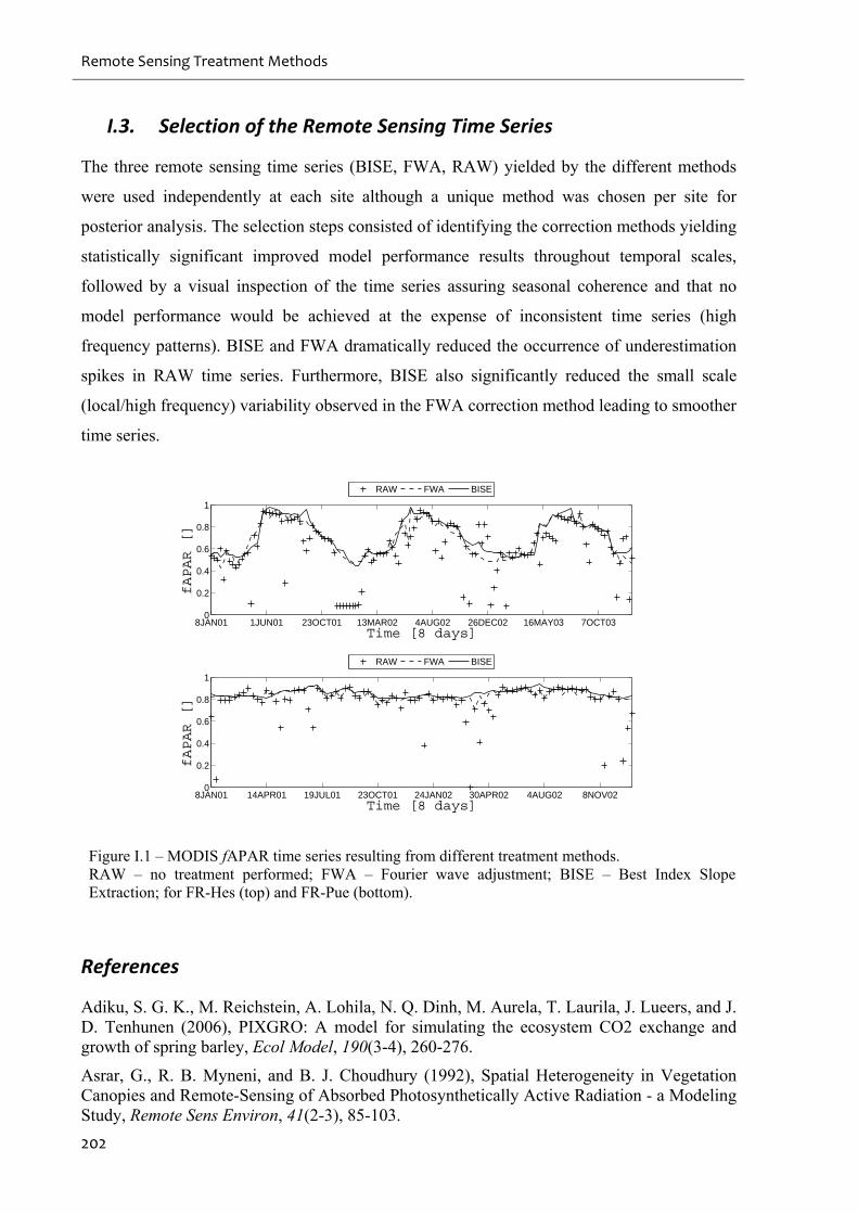
Remote Sensing Treatment Methods
202
I.3. Selection of the Remote Sensing Time Series
The three remote sensing time series (BISE, FWA, RAW) yielded by the different methods
were used independently at each site although a unique method was chosen per site for
posterior analysis. The selection steps consisted of identifying the correction methods yielding
statistically significant improved model performance results throughout temporal scales,
followed by a visual inspection of the time series assuring seasonal coherence and that no
model performance would be achieved at the expense of inconsistent time series (high
frequency patterns). BISE and FWA dramatically reduced the occurrence of underestimation
spikes in RAW time series. Furthermore, BISE also significantly reduced the small scale
(local/high frequency) variability observed in the FWA correction method leading to smoother
time series.
8JAN01 1JUN01 23OCT01 13MAR02 4AUG02 26DEC02 16MAY03 7OCT030
0.2
0.4
0.6
0.8
1
Time [8 days]
fAPAR []
RAW FWA BISE
8JAN01 14APR01 19JUL01 23OCT01 24JAN02 30APR02 4AUG02 8NOV020
0.2
0.4
0.6
0.8
1
Time [8 days]
fAPAR []
RAW FWA BISE
Figure I.1 – MODIS fAPAR time series resulting from different treatment methods. RAW – no treatment performed; FWA – Fourier wave adjustment; BISE – Best Index Slope Extraction; for FR-Hes (top) and FR-Pue (bottom).
References
Adiku, S. G. K., M. Reichstein, A. Lohila, N. Q. Dinh, M. Aurela, T. Laurila, J. Lueers, and J. D. Tenhunen (2006), PIXGRO: A model for simulating the ecosystem CO2 exchange and growth of spring barley, Ecol Model, 190(3-4), 260-276.
Asrar, G., R. B. Myneni, and B. J. Choudhury (1992), Spatial Heterogeneity in Vegetation Canopies and Remote-Sensing of Absorbed Photosynthetically Active Radiation - a Modeling Study, Remote Sens Environ, 41(2-3), 85-103.
References
203
Cook, B. I., T. M. Smith, and M. E. Mann (2005), The North Atlantic Oscillation and regional phenology prediction over europe, Global Change Biol, 11(6), 919-926.
Huete, A., K. Didan, T. Miura, E. P. Rodriguez, X. Gao, and L. G. Ferreira (2002), Overview of the radiometric and biophysical performance of the MODIS vegetation indices, Remote Sens Environ, 83(1-2), 195-213.
Huete, A. R., H. Q. Liu, K. Batchily, and W. vanLeeuwen (1997), A comparison of vegetation indices global set of TM images for EOS-MODIS, Remote Sens Environ, 59(3), 440-451.
Jenkins, J. P., A. D. Richardson, B. H. Braswell, S. V. Ollinger, D. Y. Hollinger, and M. L. Smith (2007), Refining light-use efficiency calculations for a deciduous forest canopy using simultaneous tower-based carbon flux and radiometric measurements, Agr Forest Meteorol, 143(1-2), 64-79.
Knyazikhin, Y., J. Glassy, J. L. Privette, Y. Tian, A. Lotsch, Y. Zhang, Y. Wang, J. T. Morisette, P. Votava, R. B. Myneni, R. R. Nemani, and S. W. Running (1999), MODIS Leaf Area Index (LAI) And Fraction Of Photosynthetically Active Radiation Absorbed By Vegetation (FPAR) Product (MOD15) Algorithm Theoretical Basis Document.
Lafont, S., L. Kergoat, G. Dedieu, A. Chevillard, U. Karstens, and O. Kolle (2002), Spatial and temporal variability of land CO2 fluxes estimated with remote sensing and analysis data over western Eurasia, Tellus B, 54(5), 820-833.
Mahadevan, P., S. C. Wofsy, D. M. Matross, X. M. Xiao, A. L. Dunn, J. C. Lin, C. Gerbig, J. W. Munger, V. Y. Chow, and E. W. Gottlieb (2008), A satellite-based biosphere parameterization for net ecosystem CO2 exchange: Vegetation Photosynthesis and Respiration Model (VPRM), Global Biogeochem Cy, 22(2), doi:10.1029/2006GB002735.
Miglietta, F., B. Gioli, R. W. A. Hutjes, and M. Reichstein (2006), Net regional ecosystem CO2 exchange from airborne and ground-based eddy covariance, land-use maps and weather observations, Global Change Biol, 12(1-13).
Myneni, R. B., R. R. Nemani, and S. W. Running (1997), Estimation of global leaf area index and absorbed par using radiative transfer models, Ieee T Geosci Remote, 35(6), 1380-1393.
Myneni, R. B., S. Hoffman, Y. Knyazikhin, J. L. Privette, J. Glassy, Y. Tian, Y. Wang, X. Song, Y. Zhang, G. R. Smith, A. Lotsch, M. Friedl, J. T. Morisette, P. Votava, R. R. Nemani, and S. W. Running (2002), Global products of vegetation leaf area and fraction absorbed PAR from year one of MODIS data, Remote Sens Environ, 83(1-2), 214-231.
Potter, C. S., E. A. Davidson, S. A. Klooster, D. C. Nepstad, G. H. De Negreiros, and V. Brooks (1998), Regional application of an ecosystem production model for studies of biogeochemistry in Brazilian Amazonia, Global Change Biol, 4(3), 315-333.
Reichstein, M., P. Ciais, D. Papale, R. Valentini, S. Running, N. Viovy, W. Cramer, A. Granier, J. Ogee, V. Allard, M. Aubinet, C. Bernhofer, N. Buchmann, A. Carrara, T. Grunwald, M. Heimann, B. Heinesch, A. Knohl, W. Kutsch, D. Loustau, G. Manca, G. Matteucci, F. Miglietta, J. M. Ourcival, K. Pilegaard, J. Pumpanen, S. Rambal, S. Schaphoff, G. Seufert, J. F. Soussana, M. J. Sanz, T. Vesala, and M. Zhao (2007), Reduction of ecosystem productivity and respiration during the European summer 2003 climate anomaly: a joint flux tower, remote sensing and modelling analysis, Global Change Biol, 13(3), 634-651.
Seaquist, J. W., L. Olsson, and J. Ardo (2003), A remote sensing-based primary production model for grassland biomes, Ecol Model, 169(1), 131-155.
Sellers, P. J., S. O. Los, C. J. Tucker, C. O. Justice, D. A. Dazlich, G. J. Collatz, and D. A. Randall (1996), A revised land surface parameterization (SiB2) for atmospheric GCMs .2.
Remote Sensing Treatment Methods
204
The generation of global fields of terrestrial biophysical parameters from satellite data, J Climate, 9(4), 706-737.
Veroustraete, F., J. Patyn, and R. B. Myneni (1996), Estimating net ecosystem exchange of carbon using the normalized difference vegetation index and an ecosystem model, Remote Sens Environ, 58(1), 115-130.
Viovy, N., O. Arino, and A. S. Belward (1992), The Best Index Slope Extraction (Bise) - a Method for Reducing Noise in NDVI Time-Series, Int J Remote Sens, 13(8), 1585-1590.
Wang, Q., J. Tenhunen, N. Q. Dinh, M. Reichstein, T. Vesala, and P. Keronen (2004), Similarities in ground- and satellite-based NDVI time series and their relationship to physiological activity of a Scots pine forest in Finland, Remote Sens Environ, 93(1-2), 225-237.
Xiao, X. M., D. Hollinger, J. Aber, M. Goltz, E. A. Davidson, Q. Y. Zhang, and B. Moore (2004a), Satellite-based modeling of gross primary production in an evergreen needleleaf forest, Remote Sens Environ, 89(4), 519-534.
Xiao, X. M., Q. Y. Zhang, B. Braswell, S. Urbanski, S. Boles, S. Wofsy, M. Berrien, and D. Ojima (2004b), Modeling gross primary production of temperate deciduous broadleaf forest using satellite images and climate data, Remote Sens Environ, 91(2), 256-270.
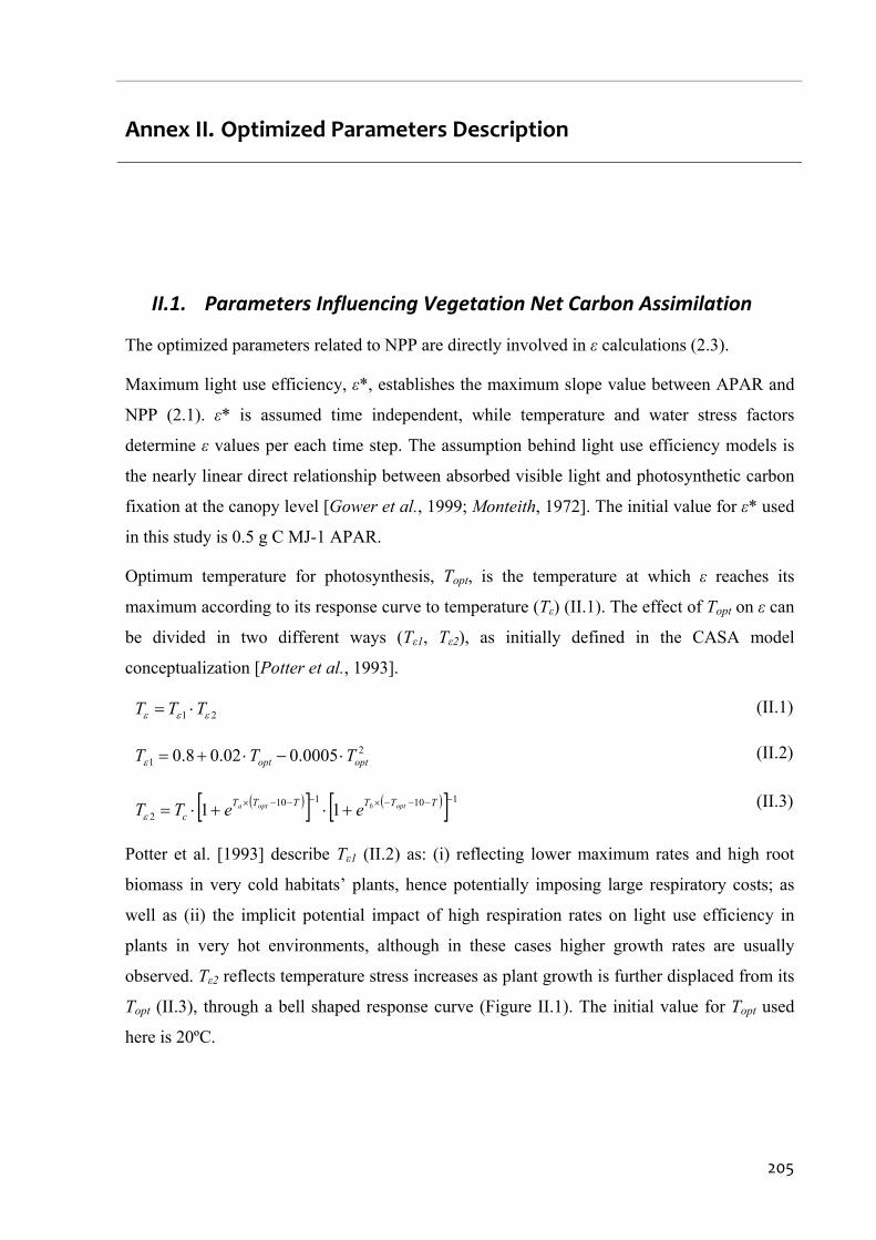
205
Annex II. Optimized Parameters Description
II.1. Parameters Influencing Vegetation Net Carbon Assimilation
The optimized parameters related to NPP are directly involved in ε calculations (2.3).
Maximum light use efficiency, ε*, establishes the maximum slope value between APAR and
NPP (2.1). ε* is assumed time independent, while temperature and water stress factors
determine ε values per each time step. The assumption behind light use efficiency models is
the nearly linear direct relationship between absorbed visible light and photosynthetic carbon
fixation at the canopy level [Gower et al., 1999; Monteith, 1972]. The initial value for ε* used
in this study is 0.5 g C MJ-1 APAR.
Optimum temperature for photosynthesis, Topt, is the temperature at which ε reaches its
maximum according to its response curve to temperature (Tε) (II.1). The effect of Topt on ε can
be divided in two different ways (Tε1, Tε2), as initially defined in the CASA model
conceptualization [Potter et al., 1993].
21 TTT (II.1)
21 0005.002.08.0 optopt TTT (II.2)
1101102 11
TTTTTTc
optbopta eeTT (II.3)
Potter et al. [1993] describe Tε1 (II.2) as: (i) reflecting lower maximum rates and high root
biomass in very cold habitats’ plants, hence potentially imposing large respiratory costs; as
well as (ii) the implicit potential impact of high respiration rates on light use efficiency in
plants in very hot environments, although in these cases higher growth rates are usually
observed. Tε2 reflects temperature stress increases as plant growth is further displaced from its
Topt (II.3), through a bell shaped response curve (Figure II.1). The initial value for Topt used
here is 20ºC.
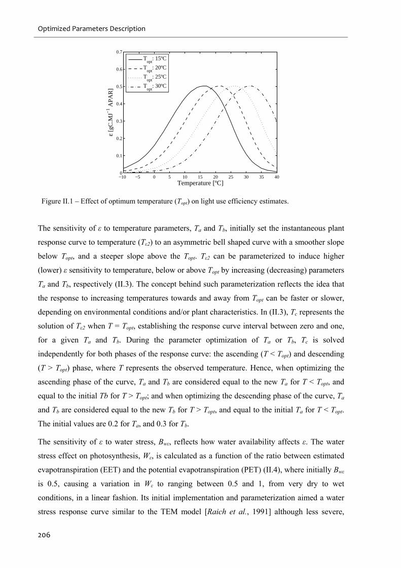
Optimized Parameters Description
206
−10 −5 0 5 10 15 20 25 30 35 400
0.1
0.2
0.3
0.4
0.5
0.6
0.7
Temperature [ºC]
ε [g
C.M
J−1 A
PAR
]
T
opt: 15ºC
Topt
: 20ºC
Topt
: 25ºC
Topt
: 30ºC
Figure II.1 – Effect of optimum temperature (Topt) on light use efficiency estimates.
The sensitivity of ε to temperature parameters, Ta and Tb, initially set the instantaneous plant
response curve to temperature (Tε2) to an asymmetric bell shaped curve with a smoother slope
below Topt, and a steeper slope above the Topt. Tε2 can be parameterized to induce higher
(lower) ε sensitivity to temperature, below or above Topt by increasing (decreasing) parameters
Ta and Tb, respectively (II.3). The concept behind such parameterization reflects the idea that
the response to increasing temperatures towards and away from Topt can be faster or slower,
depending on environmental conditions and/or plant characteristics. In (II.3), Tc represents the
solution of Tε2 when T = Topt, establishing the response curve interval between zero and one,
for a given Ta and Tb. During the parameter optimization of Ta or Tb, Tc is solved
independently for both phases of the response curve: the ascending (T < Topt) and descending
(T > Topt) phase, where T represents the observed temperature. Hence, when optimizing the
ascending phase of the curve, Ta and Tb are considered equal to the new Ta for T < Topt, and
equal to the initial Tb for T > Topt; and when optimizing the descending phase of the curve, Ta
and Tb are considered equal to the new Tb for T > Topt, and equal to the initial Ta for T < Topt.
The initial values are 0.2 for Ta, and 0.3 for Tb.
The sensitivity of ε to water stress, Bwε, reflects how water availability affects ε. The water
stress effect on photosynthesis, Wε, is calculated as a function of the ratio between estimated
evapotranspiration (EET) and the potential evapotranspiration (PET) (II.4), where initially Bwε
is 0.5, causing a variation in Wε to ranging between 0.5 and 1, from very dry to wet
conditions, in a linear fashion. Its initial implementation and parameterization aimed a water
stress response curve similar to the TEM model [Raich et al., 1991] although less severe,
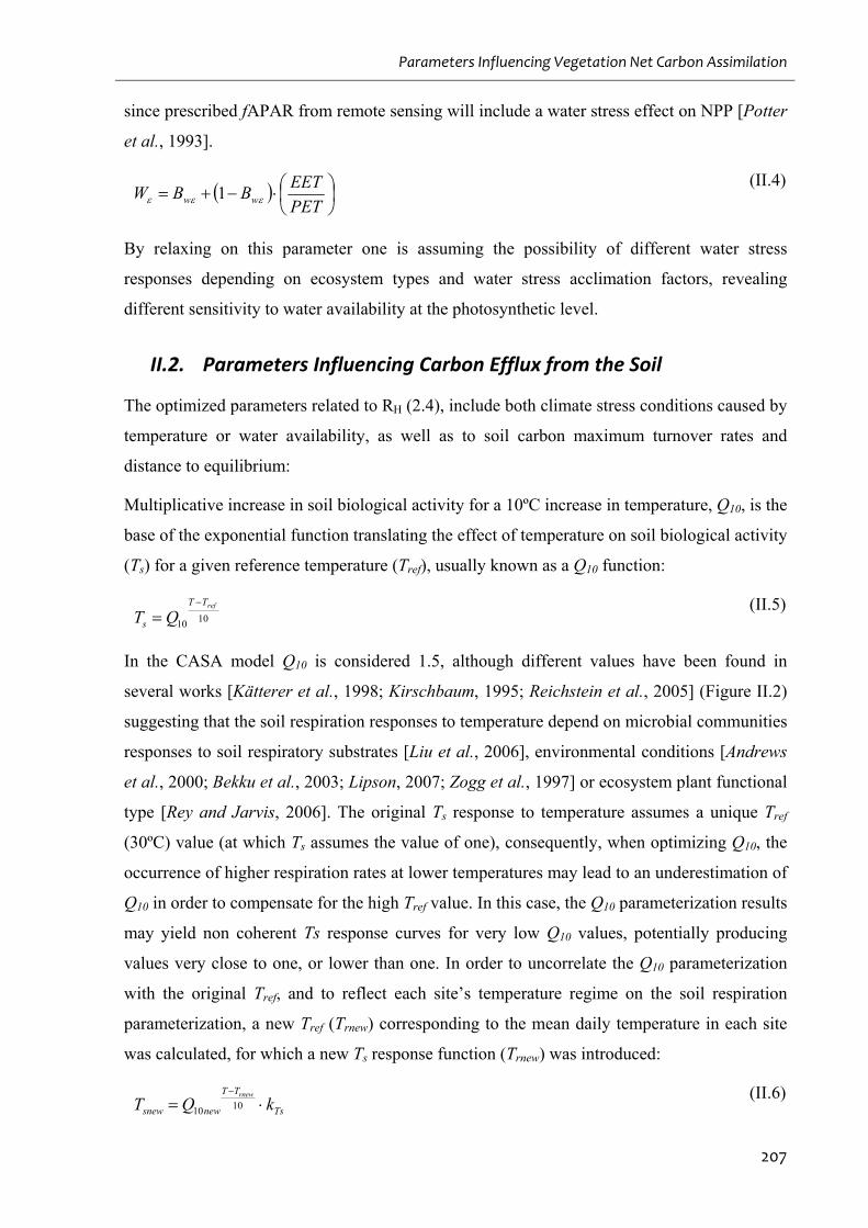
Parameters Influencing Vegetation Net Carbon Assimilation
207
since prescribed fAPAR from remote sensing will include a water stress effect on NPP [Potter
et al., 1993].
PET
EETBBW ww 1
(II.4)
By relaxing on this parameter one is assuming the possibility of different water stress
responses depending on ecosystem types and water stress acclimation factors, revealing
different sensitivity to water availability at the photosynthetic level.
II.2. Parameters Influencing Carbon Efflux from the Soil
The optimized parameters related to RH (2.4), include both climate stress conditions caused by
temperature or water availability, as well as to soil carbon maximum turnover rates and
distance to equilibrium:
Multiplicative increase in soil biological activity for a 10ºC increase in temperature, Q10, is the
base of the exponential function translating the effect of temperature on soil biological activity
(Ts) for a given reference temperature (Tref), usually known as a Q10 function:
1010
refTT
s QT
(II.5)
In the CASA model Q10 is considered 1.5, although different values have been found in
several works [Kätterer et al., 1998; Kirschbaum, 1995; Reichstein et al., 2005] (Figure II.2)
suggesting that the soil respiration responses to temperature depend on microbial communities
responses to soil respiratory substrates [Liu et al., 2006], environmental conditions [Andrews
et al., 2000; Bekku et al., 2003; Lipson, 2007; Zogg et al., 1997] or ecosystem plant functional
type [Rey and Jarvis, 2006]. The original Ts response to temperature assumes a unique Tref
(30ºC) value (at which Ts assumes the value of one), consequently, when optimizing Q10, the
occurrence of higher respiration rates at lower temperatures may lead to an underestimation of
Q10 in order to compensate for the high Tref value. In this case, the Q10 parameterization results
may yield non coherent Ts response curves for very low Q10 values, potentially producing
values very close to one, or lower than one. In order to uncorrelate the Q10 parameterization
with the original Tref, and to reflect each site’s temperature regime on the soil respiration
parameterization, a new Tref (Trnew) corresponding to the mean daily temperature in each site
was calculated, for which a new Ts response function (Trnew) was introduced:
Ts
TT
newsnew kQTrnew
1010
(II.6)
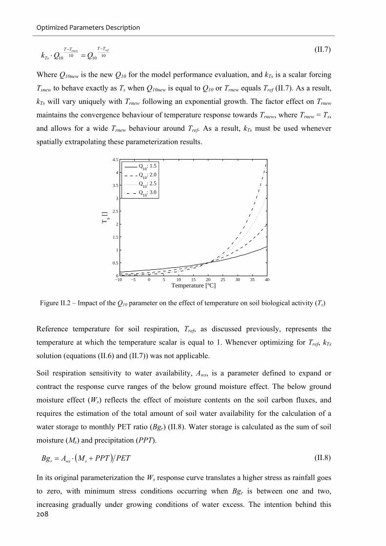
Optimized Parameters Description
208
10101010
refrnew TTTT
Ts QQk
(II.7)
Where Q10new is the new Q10 for the model performance evaluation, and kTs is a scalar forcing
Tsnew to behave exactly as Ts when Q10new is equal to Q10 or Trnew equals Tref (II.7). As a result,
kTs will vary uniquely with Trnew following an exponential growth. The factor effect on Trnew
maintains the convergence behaviour of temperature response towards Trnew, where Trnew = Ts,
and allows for a wide Trnew behaviour around Tref. As a result, kTs must be used whenever
spatially extrapolating these parameterization results.
−10 −5 0 5 10 15 20 25 30 35 400
0.5
1
1.5
2
2.5
3
3.5
4
4.5
Temperature [ºC]
Ts [
]
Q
10: 1.5
Q10
: 2.0
Q10
: 2.5
Q10
: 3.0
Figure II.2 – Impact of the Q10 parameter on the effect of temperature on soil biological activity (Ts)
Reference temperature for soil respiration, Tref, as discussed previously, represents the
temperature at which the temperature scalar is equal to 1. Whenever optimizing for Tref, kTs
solution (equations (II.6) and (II.7)) was not applicable.
Soil respiration sensitivity to water availability, Aws, is a parameter defined to expand or
contract the response curve ranges of the below ground moisture effect. The below ground
moisture effect (Ws) reflects the effect of moisture contents on the soil carbon fluxes, and
requires the estimation of the total amount of soil water availability for the calculation of a
water storage to monthly PET ratio (Bgr) (II.8). Water storage is calculated as the sum of soil
moisture (Ms) and precipitation (PPT).
PETPPTMABg swsr (II.8)
In its original parameterization the Ws response curve translates a higher stress as rainfall goes
to zero, with minimum stress conditions occurring when Bgr is between one and two,
increasing gradually under growing conditions of water excess. The intention behind this
Parameters Influencing Carbon Efflux from the Soil
209
optimization is to adjust Ws by including Aws, which affects the Bgr ranges for the different
response functions occur. Increases in Aws imply a higher sensitivity of soil carbon effluxes to
water stress conditions, although within smaller Bgr ranges. For the initial parameterization
Aws equals one, for an Aws of 3 the minimum stress conditions are observed for Bgr between
0.4 and 0.6, and for Bgr values higher than 10 Ws assumes a constant value of 0.5.
0 1 2 3 4 5 6 7 8 9 10 11 12 13 14 150
0.2
0.4
0.6
0.8
1
Bgr []
Ws [
]
Aws
=0.5
Aws
=1.0
Aws
=3.0
Figure II.3 – Sensitivity of the below ground soil moisture effect (Ws) to the water storage to monthly PET ratio (Bgr) for different Aws estimates (Ts).
Soil pools turnover rates, k, for each soil pool affect linearly the carbon efflux at each pool per
calculation, and are calculated from annual decomposition rates constants (kann) to the
temporal resolution of simulations based on the following method:
Nkannek1
1 (II.9)
Where N represents the number of time steps per year. The effect of downscaling method used
on k can be considered negligible since not only the carbon pool values at equilibrium show
low differences between different temporal resolutions, but also the carbon accumulation
development during the model initialization follows each other closely, leading to similar
spin-up periods until equilibrium. The lower kann, hence lower k, the longer both the time
required until equilibrium is reached and the larger the carbon stored in the pool. Since k
affects linearly the carbon efflux of each pool per calculation, the optimization of k entails that
the soil carbon storage capacity at equilibrium may vary, depending also on the mean climatic
regime used for spin-up, resulting in different carbon emissions from soils of different
sites/ecosystems. In the current optimization, k was not optimized independently for each soil
pool, but rather as a fraction of its initial value, constant throughout pools.
Optimized Parameters Description
210
References
Andrews, J. A., R. Matamala, K. M. Westover, and W. H. Schlesinger (2000), Temperature effects on the diversity of soil heterotrophs and the delta C-13 of soil-respired CO2, Soil Biol Biochem, 32(5), 699-706.
Bekku, Y. S., T. Nakatsubo, A. Kume, M. Adachi, and H. Koizumi (2003), Effect of warming on the temperature dependence of soil, respiration rate in arctic, temperate and tropical soils, Appl Soil Ecol, 22(3), 205-210.
Gower, S. T., C. J. Kucharik, and J. M. Norman (1999), Direct and indirect estimation of leaf area index, f(APAR), and net primary production of terrestrial ecosystems, Remote Sens Environ, 70(1), 29-51.
Kätterer, T., M. Reichstein, O. Andren, and A. Lomander (1998), Temperature dependence of organic matter decomposition: a critical review using literature data analyzed with different models, Biol Fert Soils, 27(3), 258-262.
Kirschbaum, M. U. F. (1995), The Temperature-Dependence of Soil Organic-Matter Decomposition, and the Effect of Global Warming on Soil Organic-C Storage, Soil Biol Biochem, 27(6), 753-760.
Lipson, D. A. (2007), Relationships between temperature responses and bacterial community structure along seasonal and altitudinal gradients, Fems Microbiol Ecol, 59(2), 418-427.
Liu, H. S., L. H. Li, X. G. Han, J. H. Huang, J. X. Sun, and H. Y. Wang (2006), Respiratory substrate availability plays a crucial role in the response of soil respiration to environmental factors, Appl Soil Ecol, 32(3), 284-292.
Monteith, J. L. (1972), Solar-Radiation and Productivity in Tropical Ecosystems, J Appl Ecol, 9(3), 747-766.
Potter, C. S., J. T. Randerson, C. B. Field, P. A. Matson, P. M. Vitousek, H. A. Mooney, and S. A. Klooster (1993), Terrestrial Ecosystem Production - a Process Model-Based on Global Satellite and Surface Data, Global Biogeochem Cy, 7(4), 811-841.
Raich, J. W., E. B. Rastetter, J. M. Melillo, D. W. Kicklighter, P. A. Steudler, B. J. Peterson, A. L. Grace, B. Moore, and C. J. Vorosmarty (1991), Potential Net Primary Productivity in South-America - Application of a Global-Model, Ecol Appl, 1(4), 399-429.
Reichstein, M., T. Katterer, O. Andren, P. Ciais, E. D. Schulze, W. Cramer, D. Papale, and R. Valentini (2005), Temperature sensitivity of decomposition in relation to soil organic matter pools: critique and outlook, Biogeosciences, 2(4), 317-321.
Rey, A., and P. Jarvis (2006), Modelling the effect of temperature on carbon mineralization rates across a network of European forest sites (FORCAST), Global Change Biol, 12(10), 1894-1908.
Zogg, G. P., D. R. Zak, D. B. Ringelberg, N. W. MacDonald, K. S. Pregitzer, and D. C. White (1997), Compositional and functional shifts in microbial communities due to soil warming, Soil Sci Soc Am J, 61(2), 475-481.
211
Annex III. Model Performance Evaluation Measures
The evaluation of model performance relied on four main statistical indexes, considered
complimentary on the evaluation of model performance: correlation coefficient (r2); variance
ratio (VR; (III.1)); normalized average error (NAE; (III.2)); and the model efficiency (MEF;
(III.3)). Each performance measure reveals different aspects of the model behaviour,
providing relevant information on the potential reasons behind residuals occurrence and
magnitude [Janssen and Heuberger, 1995]. In this perspective, and in the context of the
current study:
The variance ration (VR) reveals population variance dissimilarities between NEP estimates
and observations:
2
2
OBS
SIM
S
SVR ,
(III.1)
where 2OBSS and 2
SIMS stand for estimated variances of observations and simulations,
respectively. Values higher than one entail the model’s structure high sensitivity to one or
more drivers, while values lower than one imply the data-driven processes simulated by the
model are insufficient to mimic the variability in observed populations. VR values closer to
unity disclose model drivers and structure suitability in reproducing observed populations
variance. An isolated analysis of VR is insufficient to conclude on model’s misfits causes.
Yet, in association with r2 or MEF measures discloses model sensitivity changes behind
correlation or model efficiency adjustments.
The normalized average error (NAE) expresses the average model biases relatively to the
observed populations mean:
OBS
SIMOBSNAE
.
(III.2)
Here, OBS and SIM represent mean observations and simulations, respectively. Although
the expression of over or underestimations yields rather coarse information on simulations-
Model Performance Evaluation Measures
212
observations inconsistencies, it has a significant role on the current exercise in identifying the
optimized parameter sets that yield best fits to the observations.
Modelling efficiency (MEF) quantifies the relative association between estimates and
observations over the association between the observations and its mean (the nominal
situation):
N
ii
N
iii
OBSOBS
SIMOBSMEF
1
2
1
2
1 ,
(III.3)
where OBSi and SIMi correspond to the observed and simulated values, respectively; and N is
the number of observations. Negative values of MEF reveal no association between
observations and simulations and/or the association in not better than the nominal situation
(mean). A MEF value closer to 1 reveals better association between observations and
simulations (MEF = 1, implies estimates to be in the 1 to 1 line). Yet, perfect variables
association (r2 = 1) revealing an offset, yield MEF values < 1. In the current study
perspective, MEF integrates the most relevant information on model performance evaluation,
since it measures both the association between estimates and observations as well as their
coincidence, revealing sensitivity to systematic deviations between model and observation [cf.
Smith et al., 1996].
Further, the normalized mean absolute error (NMAE) is used to evaluate the vegetation
carbon pools estimates:
OBS
OBSSIM
NMAE
N
iiiN
1
1
.
(III.4)
Here, OBSi and SIMi correspond to the ith observed and simulated carbon pools values.
Throughout the text correlations can be often referred as negligible, low, etc. The absolute r
values corresponding to each “definition” are summarized in Table III.1
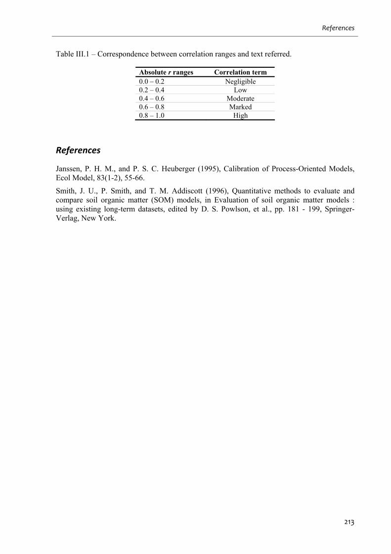
References
213
Table III.1 – Correspondence between correlation ranges and text referred.
Absolute r ranges Correlation term 0.0 – 0.2 Negligible 0.2 – 0.4 Low 0.4 – 0.6 Moderate 0.6 – 0.8 Marked 0.8 – 1.0 High
References
Janssen, P. H. M., and P. S. C. Heuberger (1995), Calibration of Process-Oriented Models, Ecol Model, 83(1-2), 55-66.
Smith, J. U., P. Smith, and T. M. Addiscott (1996), Quantitative methods to evaluate and compare soil organic matter (SOM) models, in Evaluation of soil organic matter models : using existing long-term datasets, edited by D. S. Powlson, et al., pp. 181 - 199, Springer-Verlag, New York.

215
Annex IV. Application the CCSSAr to First Order Soil C Dynamics
Models
Following the approach by Andrén and Kätterer [1997], we assume soil C dynamics can be
described by a simple two-component model based on first order kinetics:
111 CrkI
dt
dC
(IV.1)
22112 CrkCrkh
dt
dC
(IV.2)
Being: I, mean annual C inputs to the soil, k1 and k2 the decay constants of young (C1) and old
(C2) pools, respectively, and r represents external factors affecting the pools’ decomposition
rates (mainly climatic factors) The formulation allows soil C dynamics to be analytically
solved at steady state, yielding:
1,1 kr
IC ss
(IV.3)
2,2 kr
IhC ss
(IV.4)
Being C1,ss and C2,ss the C1 and C2 pools at steady state. Assuming that in non steady-state
conditions: ssns CC ,2,2 ; and that except C2, all other pools (including the vegetation pools)
are in steady state then: dt
dCNEP 2 (IV.5); and GPPfNPPI [Waring et al., 1998]. We
can then solve equation (IV.6) for η:
rk
GPPfhrk
rk
GPPfrkhNEP
22
11
(IV.5)
GPPfhNEP 1 (IV.6)
GPPf
NEP
h
11
(IV.7)
Application the CCSSAr to First Order Soil C Dynamics Models
216
Equation (IV.7) yields 1 under steady-state conditions ( 0NEP ) and shows an inverse
relationship with GPPfNEP (positive values for sources and negative values for sinks).
The current formulation exemplifies the potential generalization of the relaxed steady-state
approach using a simple model concept for the purpose. Although the current assumptions
represent strong limitations to observations, they represent general explicit or implicit
assumptions in biogeochemical modelling spin-up routines. We consider formulations to be
model specific allowing for significant improvements in CCSSAr applications.
References
Andrén, O., and T. Kätterer (1997), ICBM: The introductory carbon balance model for exploration of soil carbon balances, Ecol Appl, 7(4), 1226-1236.
Waring, R. H., J. J. Landsberg, and M. Williams (1998), Net primary production of forests: a constant fraction of gross primary production?, Tree Physiol, 18(2), 129-134.
217
Annex V. Adjusting the CASA Model for Explicitly Estimating RA
V.1. Explicitly Calculating RA
In the original CASA model [Potter et al., 1993] NEP is estimated as the difference between
NPP and heterotrophic respiration RH:
HRNPPNEP , (V.1)
where NPP is calculated as a function of absorbed photosynthetically active radiation (APAR)
and light use efficiency (ε):
APARNPP . (V.2)
APAR is calculated as the product between fraction of photosynthetically active radiation
absorbed by vegetation (fAPAR) and the amount of photosynthetically active radiation (PAR):
PARfAPARAPAR . (V.3)
ε is calculated by down-regulating maximum light use efficiency (ε*) via the effect of
temperature (Tε) and water (Wε) stress factors:
WT * , (V.4)
where Tε follows a bell shaped response curve peaking at an optimum temperature and Wε
responds linearly to water availability. The new formulation, CASAG, proposes to calculate
NPP as the difference between GPP and RA
ARGPPNPP , (V.5)
an approach also commonly used in biogeochemical modelling [Ruimy et al., 1999]. The main
conceptual transition between both approaches is the assumption that RA is not a constant
fraction of GPP, entailing that the carbon use efficiency of the vegetation (CUE=NPP/GPP)
varies from site to site [e.g. DeLucia et al., 2007; Litton et al., 2007]. Further, for consistency,
we assume that GPP also follows the radiation use efficiency approach [Monteith, 1972]:
gAPARGPP . (V.6)
Adjusting the CASA Model for Explicitly Estimating RA
218
Here, we differentiate between light use efficiency of NPP (ε) and for GPP (εg).
We follow Thornley’s [1970] conceptualization for RA, generally formulated as the sum
between maintenance (RM) and growth (RG) respiration:
GMA RRR , (V.7)
where RM is considered proportional to the vegetation carbon content:
dMGM CkYR 1 , (V.8)
and RG to the proportion of immediate carbon supply (GPP):
GPPYR GG 1 . (V.9)
The implementation of the RA model consists on an adaptation from Thornley and Cannell
[2000], where a constant fraction of growth is degradable. Plant tissue is partitioned into non-
degradable and degradable mass – only the latest subject to maintenance costs. Above, YG is
the growth efficiency (0.75, [Hunt, 1994; Prince and Goward, 1995; Rambal et al., 2004]); Cd
is degradable C, and kM a maintenance respiration coefficient. We considered fd MCC ,
where Mf is the metabolic fraction of the pool, prescribed per plant functional type (PFT)
within the CASA model [Potter et al., 1993]. The maintenance respiration coefficient (kM) is
considered both: (i) temperature dependent; and (ii) better related to plant nitrogen content (N)
than to plant C [although not always, but see Amthor, 2000, and references herein]. Usual
values for the temperature dependence of maintenance respiration consider Q10 around 2.0
[Amthor, 2000], although values can range between 1.4 and 2.5 [Ryan et al., 1996]. Ryan
[1991] estimated a maintenance respiration coefficient in terms of N (kM,N) of 0.2181 gC.gN-
1.d-1 for a reference temperature of 20ºC. Conversion from C to N is based on the C/N ratios
of the different pools. Carbon-to-nitrogen ratios of live vegetation pools are considered equal
to the C/N of the metabolic component of litter pools in Potter et al. [1993] for leaf and root
pools (25); while of wood pool are considered identical between dead and live pools (260).
Carbon allocation to the main vegetation pools (root, wood and leaf) follows the scheme
proposed by Friedlingstein et al. [1999] in which the partitioning of carbon through the
different tissue compartments changes with resources availability. In the modified version of
CASA (from here on identified as CASAG) root pools were divided in coarse and fine roots
(Figure 3.1). Allocation of C to root pools was partitioned into coarse (25%) and fine (75%).
Root pool partitioning aims at the consideration of a slow belowground live vegetation pool –
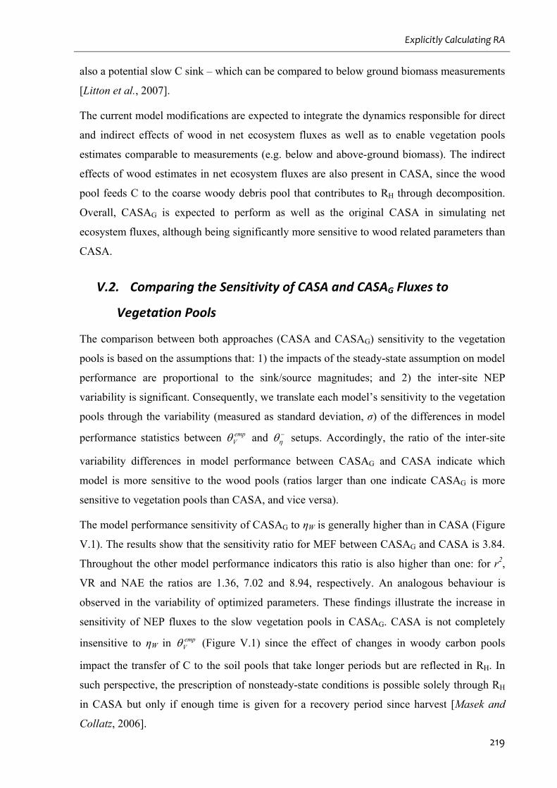
Explicitly Calculating RA
219
also a potential slow C sink – which can be compared to below ground biomass measurements
[Litton et al., 2007].
The current model modifications are expected to integrate the dynamics responsible for direct
and indirect effects of wood in net ecosystem fluxes as well as to enable vegetation pools
estimates comparable to measurements (e.g. below and above-ground biomass). The indirect
effects of wood estimates in net ecosystem fluxes are also present in CASA, since the wood
pool feeds C to the coarse woody debris pool that contributes to RH through decomposition.
Overall, CASAG is expected to perform as well as the original CASA in simulating net
ecosystem fluxes, although being significantly more sensitive to wood related parameters than
CASA.
V.2. Comparing the Sensitivity of CASA and CASAG Fluxes to
Vegetation Pools
The comparison between both approaches (CASA and CASAG) sensitivity to the vegetation
pools is based on the assumptions that: 1) the impacts of the steady-state assumption on model
performance are proportional to the sink/source magnitudes; and 2) the inter-site NEP
variability is significant. Consequently, we translate each model’s sensitivity to the vegetation
pools through the variability (measured as standard deviation, σ) of the differences in model
performance statistics between empV and
setups. Accordingly, the ratio of the inter-site
variability differences in model performance between CASAG and CASA indicate which
model is more sensitive to the wood pools (ratios larger than one indicate CASAG is more
sensitive to vegetation pools than CASA, and vice versa).
The model performance sensitivity of CASAG to ηW is generally higher than in CASA (Figure
V.1). The results show that the sensitivity ratio for MEF between CASAG and CASA is 3.84.
Throughout the other model performance indicators this ratio is also higher than one: for r2,
VR and NAE the ratios are 1.36, 7.02 and 8.94, respectively. An analogous behaviour is
observed in the variability of optimized parameters. These findings illustrate the increase in
sensitivity of NEP fluxes to the slow vegetation pools in CASAG. CASA is not completely
insensitive to ηW in empV (Figure V.1) since the effect of changes in woody carbon pools
impact the transfer of C to the soil pools that take longer periods but are reflected in RH. In
such perspective, the prescription of nonsteady-state conditions is possible solely through RH
in CASA but only if enough time is given for a recovery period since harvest [Masek and
Collatz, 2006].
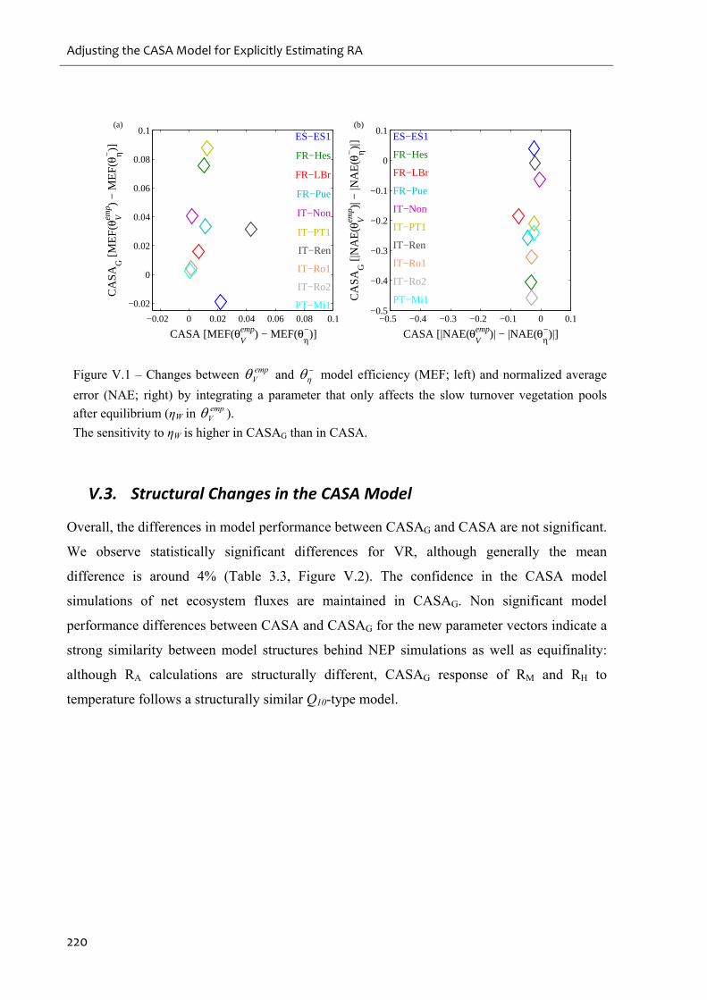
Adjusting the CASA Model for Explicitly Estimating RA
220
−0.02 0 0.02 0.04 0.06 0.08 0.1
−0.02
0
0.02
0.04
0.06
0.08
0.1ES−ES1
FR−Hes
FR−LBr
FR−Pue
IT−Non
IT−PT1
IT−Ren
IT−Ro1
IT−Ro2
PT−Mi1
CASA [MEF(θVemp) − MEF(θ
η−)]
CA
SAG
[M
EF(
θ Vemp )
− M
EF(
θ η−)]
−0.5 −0.4 −0.3 −0.2 −0.1 0 0.1−0.5
−0.4
−0.3
−0.2
−0.1
0
0.1 ES−ES1
FR−Hes
FR−LBr
FR−Pue
IT−Non
IT−PT1
IT−Ren
IT−Ro1
IT−Ro2
PT−Mi1
CASA [|NAE(θVemp)| − |NAE(θ
η−)|]
CA
SAG
[|N
AE
(θVem
p )| −
|NA
E(θ
η−)|]
(a) (b)
Figure V.1 – Changes between empV and
model efficiency (MEF; left) and normalized average
error (NAE; right) by integrating a parameter that only affects the slow turnover vegetation pools
after equilibrium (ηW in empV ).
The sensitivity to ηW is higher in CASAG than in CASA.
V.3. Structural Changes in the CASA Model
Overall, the differences in model performance between CASAG and CASA are not significant.
We observe statistically significant differences for VR, although generally the mean
difference is around 4% (Table 3.3, Figure V.2). The confidence in the CASA model
simulations of net ecosystem fluxes are maintained in CASAG. Non significant model
performance differences between CASA and CASAG for the new parameter vectors indicate a
strong similarity between model structures behind NEP simulations as well as equifinality:
although RA calculations are structurally different, CASAG response of RM and RH to
temperature follows a structurally similar Q10-type model.
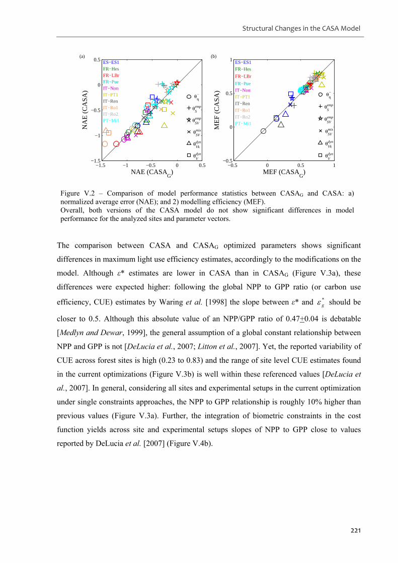
Structural Changes in the CASA Model
221
−1.5 −1 −0.5 0 0.5−1.5
−1
−0.5
0
0.5
NAE (CASAG
)
NA
E (
CA
SA
)
ES−ES1 FR−Hes FR−LBr FR−Pue IT−Non IT−PT1 IT−Ren IT−Ro1 IT−Ro2 PT−Mi1
θV dyn
θVkdyn
θSVmix
θSVemp
θS emp
θη −
−0.5 0 0.5 1−0.5
0
0.5
1
MEF (CASAG
)
ME
F (
CA
SA
)
ES−ES1
FR−Hes
FR−LBr
FR−Pue IT−Non IT−PT1 IT−Ren
IT−Ro1 IT−Ro2 PT−Mi1
θV dyn
θVkdyn
θSVmix
θSVemp
θS emp
θη −
(a) (b)
Figure V.2 – Comparison of model performance statistics between CASAG and CASA: a) normalized average error (NAE); and 2) modelling efficiency (MEF). Overall, both versions of the CASA model do not show significant differences in model performance for the analyzed sites and parameter vectors.
The comparison between CASA and CASAG optimized parameters shows significant
differences in maximum light use efficiency estimates, accordingly to the modifications on the
model. Although ε* estimates are lower in CASA than in CASAG (Figure V.3a), these
differences were expected higher: following the global NPP to GPP ratio (or carbon use
efficiency, CUE) estimates by Waring et al. [1998] the slope between ε* and *g should be
closer to 0.5. Although this absolute value of an NPP/GPP ratio of 0.47+0.04 is debatable
[Medlyn and Dewar, 1999], the general assumption of a global constant relationship between
NPP and GPP is not [DeLucia et al., 2007; Litton et al., 2007]. Yet, the reported variability of
CUE across forest sites is high (0.23 to 0.83) and the range of site level CUE estimates found
in the current optimizations (Figure V.3b) is well within these referenced values [DeLucia et
al., 2007]. In general, considering all sites and experimental setups in the current optimization
under single constraints approaches, the NPP to GPP relationship is roughly 10% higher than
previous values (Figure V.3a). Further, the integration of biometric constraints in the cost
function yields across site and experimental setups slopes of NPP to GPP close to values
reported by DeLucia et al. [2007] (Figure V.4b).
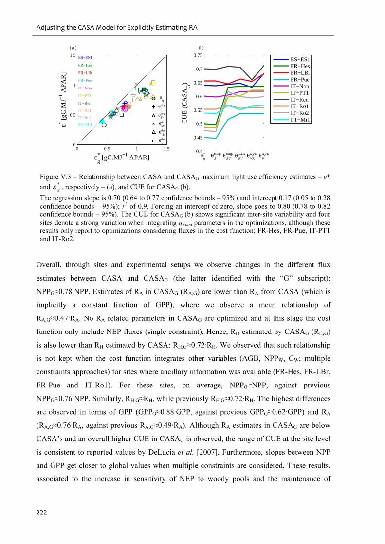
Adjusting the CASA Model for Explicitly Estimating RA
222
0 0.5 1 1.50
0.5
1
1.5
ε*g [gC.MJ−1 APAR]
ε* [gC
.MJ−
1 APA
R]
ES−ES1
FR−Hes
FR−LBr
FR−Pue
IT−Non
IT−PT1
IT−Ren
IT−Ro1
IT−Ro2
PT−Mi1
θV dyn
θVkdyn
θSVmix
θSVemp
θS emp
θη −
0.4
0.45
0.5
0.55
0.6
0.65
0.7
0.75
CU
E (
CA
SAG
)
θη − θ
S emp θ
SVemp θ
SVmix θ
Vkdyn θ
V dyn
ES−ES1FR−HesFR−LBrFR−PueIT−NonIT−PT1IT−RenIT−Ro1IT−Ro2PT−Mi1
(a) (b)
Figure V.3 – Relationship between CASA and CASAG maximum light use efficiency estimates – ε*
and *g , respectively – (a), and CUE for CASAG (b).
The regression slope is 0.70 (0.64 to 0.77 confidence bounds – 95%) and intercept 0.17 (0.05 to 0.28 confidence bounds – 95%); r2 of 0.9. Forcing an intercept of zero, slope goes to 0.80 (0.78 to 0.82 confidence bounds – 95%). The CUE for CASAG (b) shows significant inter-site variability and four sites denote a strong variation when integrating ηwood parameters in the optimizations, although these results only report to optimizations considering fluxes in the cost function: FR-Hes, FR-Pue, IT-PT1 and IT-Ro2.
Overall, through sites and experimental setups we observe changes in the different flux
estimates between CASA and CASAG (the latter identified with the “G” subscript):
NPPG≈0.78·NPP. Estimates of RA in CASAG (RA,G) are lower than RA from CASA (which is
implicitly a constant fraction of GPP), where we observe a mean relationship of
RA,G≈0.47·RA. No RA related parameters in CASAG are optimized and at this stage the cost
function only include NEP fluxes (single constraint). Hence, RH estimated by CASAG (RH,G)
is also lower than RH estimated by CASA: RH,G≈0.72·RH. We observed that such relationship
is not kept when the cost function integrates other variables (AGB, NPPW, CW; multiple
constraints approaches) for sites where ancillary information was available (FR-Hes, FR-LBr,
FR-Pue and IT-Ro1). For these sites, on average, NPPG≈NPP, against previous
NPPG≈0.76·NPP. Similarly, RH,G≈RH, while previously RH,G≈0.72·RH. The highest differences
are observed in terms of GPP (GPPG≈0.88·GPP, against previous GPPG≈0.62·GPP) and RA
(RA,G≈0.76·RA, against previous RA,G≈0.49·RA). Although RA estimates in CASAG are below
CASA’s and an overall higher CUE in CASAG is observed, the range of CUE at the site level
is consistent to reported values by DeLucia et al. [2007]. Furthermore, slopes between NPP
and GPP get closer to global values when multiple constraints are considered. These results,
associated to the increase in sensitivity of NEP to woody pools and the maintenance of
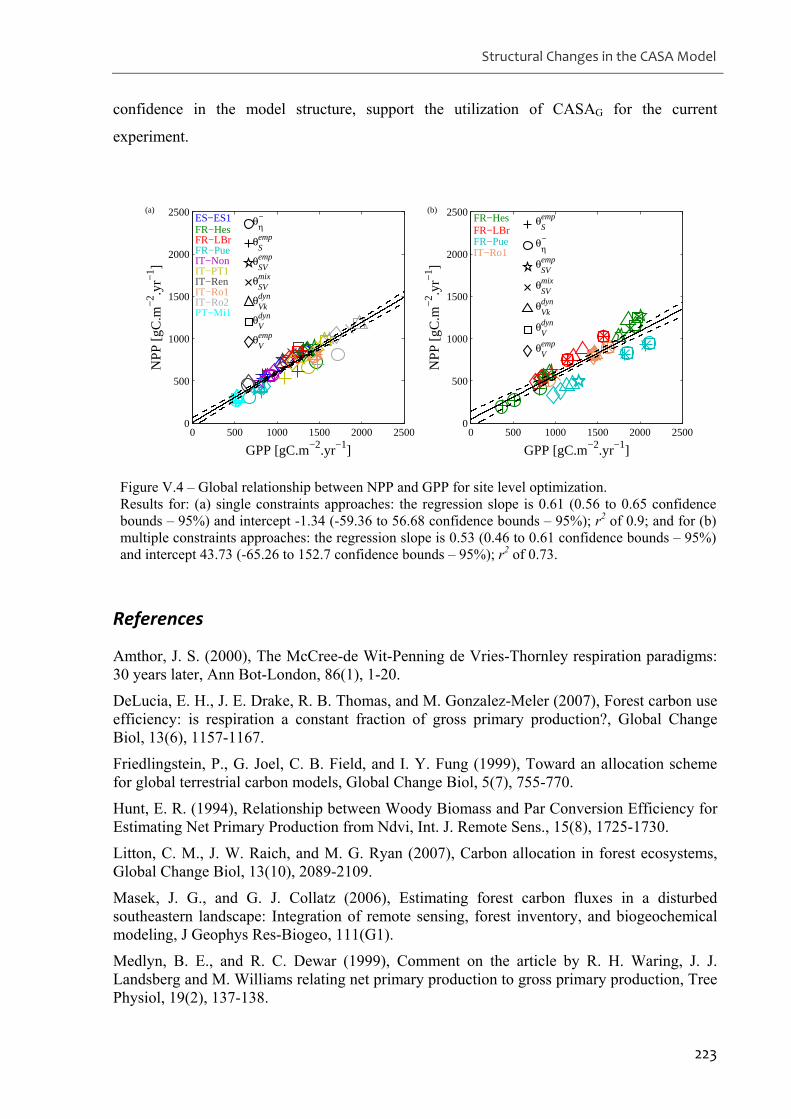
Structural Changes in the CASA Model
223
confidence in the model structure, support the utilization of CASAG for the current
experiment.
0 500 1000 1500 2000 25000
500
1000
1500
2000
2500
NPP
[gC
.m−2
.yr−1
]
GPP [gC.m−2.yr−1]
ES−ES1 FR−Hes FR−LBr FR−Pue IT−Non IT−PT1 IT−Ren IT−Ro1 IT−Ro2 PT−Mi1
θη −
θS emp
θSVemp
θSVmix
θVkdyn
θV dyn
θV emp
0 500 1000 1500 2000 25000
500
1000
1500
2000
2500
NPP
[gC
.m−2
.yr−1
]GPP [gC.m−2.yr−1]
FR−Hes FR−LBr FR−Pue IT−Ro1
θS emp
θη −
θSVemp
θSVmix
θVkdyn
θV dyn
θV emp
(a) (b)
Figure V.4 – Global relationship between NPP and GPP for site level optimization. Results for: (a) single constraints approaches: the regression slope is 0.61 (0.56 to 0.65 confidence bounds – 95%) and intercept -1.34 (-59.36 to 56.68 confidence bounds – 95%); r2 of 0.9; and for (b) multiple constraints approaches: the regression slope is 0.53 (0.46 to 0.61 confidence bounds – 95%) and intercept 43.73 (-65.26 to 152.7 confidence bounds – 95%); r2 of 0.73.
References
Amthor, J. S. (2000), The McCree-de Wit-Penning de Vries-Thornley respiration paradigms: 30 years later, Ann Bot-London, 86(1), 1-20.
DeLucia, E. H., J. E. Drake, R. B. Thomas, and M. Gonzalez-Meler (2007), Forest carbon use efficiency: is respiration a constant fraction of gross primary production?, Global Change Biol, 13(6), 1157-1167.
Friedlingstein, P., G. Joel, C. B. Field, and I. Y. Fung (1999), Toward an allocation scheme for global terrestrial carbon models, Global Change Biol, 5(7), 755-770.
Hunt, E. R. (1994), Relationship between Woody Biomass and Par Conversion Efficiency for Estimating Net Primary Production from Ndvi, Int. J. Remote Sens., 15(8), 1725-1730.
Litton, C. M., J. W. Raich, and M. G. Ryan (2007), Carbon allocation in forest ecosystems, Global Change Biol, 13(10), 2089-2109.
Masek, J. G., and G. J. Collatz (2006), Estimating forest carbon fluxes in a disturbed southeastern landscape: Integration of remote sensing, forest inventory, and biogeochemical modeling, J Geophys Res-Biogeo, 111(G1).
Medlyn, B. E., and R. C. Dewar (1999), Comment on the article by R. H. Waring, J. J. Landsberg and M. Williams relating net primary production to gross primary production, Tree Physiol, 19(2), 137-138.
Adjusting the CASA Model for Explicitly Estimating RA
224
Monteith, J. L. (1972), Solar-Radiation and Productivity in Tropical Ecosystems, J Appl Ecol, 9(3), 747-766.
Potter, C. S., J. T. Randerson, C. B. Field, P. A. Matson, P. M. Vitousek, H. A. Mooney, and S. A. Klooster (1993), Terrestrial Ecosystem Production - a Process Model-Based on Global Satellite and Surface Data, Global Biogeochem Cy, 7(4), 811-841.
Prince, S. D., and S. N. Goward (1995), Global primary production: A remote sensing approach, J Biogeogr, 22(4-5), 815-835.
Rambal, S., R. Joffre, J. M. Ourcival, J. Cavender-Bares, and A. Rocheteau (2004), The growth respiration component in eddy CO2 flux from a Quercus ilex mediterranean forest, Global Change Biol, 10(9), 1460-1469.
Ruimy, A., L. Kergoat, A. Bondeau, and Participants Potsdam NPP Model Intercomparison (1999), Comparing global models of terrestrial net primary productivity (NPP): analysis of differences in light absorption and light-use efficiency, Global Change Biol, 5, 56-64.
Ryan, M. G. (1991), Effects of Climate Change on Plant Respiration, Ecol Appl, 1(2), 157-167.
Ryan, M. G., R. M. Hubbard, S. Pongracic, R. J. Raison, and R. E. McMurtrie (1996), Foliage, fine-root, woody-tissue and stand respiration in Pinus radiata in relation to nitrogen status, Tree Physiol, 16(3), 333-343.
Thornley, J. H. M. (1970), Respiration, Growth and Maintenance in Plants, Nature, 227(5255), 304-305.
Thornley, J. H. M., and M. G. R. Cannell (2000), Modelling the components of plant respiration: Representation and realism, Ann Bot-London, 85(1), 55-67.
Waring, R. H., J. J. Landsberg, and M. Williams (1998), Net primary production of forests: a constant fraction of gross primary production?, Tree Physiol, 18(2), 129-134.
225
Annex VI. Summary of the Optimization Approach
VI.1. The Levenberg Marquardt Algorithm
The optimizations rely on the Levenberg-Marquardt algorithm (LMA) that was initialized by
Levenberg [1944] and developed by Marquardt [1963], consisting on an optimization method
that searches for the minimum of a cost function expressed as the sum of squares of non-linear
functions. The search direction is given by the solution of:
θSIM-OBSδ TT JλIJJ , (VI.1)
where J denotes the Jacobian matrix, λ is a nonnegative scalar, I is the identity matrix and δ is
the correction to the parameter vector θ towards the minimization of Ω; the T superscript
denotes a matrix transposition [Marquardt, 1963]. Depending on the magnitude of λ the LMA
can show a behaviour similar to: (i) the Gauss-Newton search method [Hartley, 1961] (when
λ→0), closing in on the converged values rapidly after the vicinity of the converged values
has been reached; and (ii) to gradient methods (when λ→∞) enabling convergence from an
initial guess that may be outside the region of convergence of other methods [Marquardt,
1963]. These two characteristics were considered essential in the choice of the LMA, as well
as its successful performance for nonlinear least squares problems in environmental sciences.
VI.2. Integrating Multiple Constraints in the Cost Function
The integration of pools and fluxes in the cost function (Ω) construction follows a weighting
approach analogous to Wang et al. [2001]:
N
jj
1
, (VI.2)
where the global cost function, Ω, results from the summation of the N partial cost functions,
Ωj, each considering a single variable constraint: NEP, AGB, NPPW or CW. We integrated a
maximum of two constraints in the cost function. Each partial cost function is defined as the
following sum of squares:
Summary of the Optimization Approach
226
jn
ijiji
j
j SIMOBSw 1
2,,2
1Ω ,
(VI.3)
where OBSi,j, (SIMi,j) is the ith observation (model estimate) of the jth constraint; and wj is the
normalization factor of the jth constraint. The normalization factors (wj) were attributed
according to the units of each variable: AGB and CW pools are divided by tree age times the
number of yearly observations; while fluxes are divided by the number of years of
observations. This normalization aims to balance the weight of fluxes and pools in the cost
function. The squared sum of all normalized misfits of each variable in the cost function
yields units of (gC m-2 yr-1)2; consequently, each partial cost matches one year of squared
residuals for all nj misfits contributing to one annual value estimate.
References
Hartley, H. O. (1961), Modified Gauss-Newton Method for Fitting of Non-Linear Regression Functions by Least Squares, Technometrics, 3(2), 269-280.
Levenberg, K. (1944), A method for the solution of certain non-linear problems in least squares, Q. Appl. Math., 2, 164-168.
Marquardt, D. W. (1963), An Algorithm for Least-Squares Estimation of Nonlinear Parameters, J Soc Ind Appl Math, 11(2), 431-441.
Wang, Y. P., R. Leuning, H. A. Cleugh, and P. A. Coppin (2001), Parameter estimation in surface exchange models using nonlinear inversion: how many parameters can we estimate and which measurements are most useful?, Global Change Biol, 7(5), 495-510.