Nutrient limitation for coastal areas and estuaries in … · Nutrient limitation for coastal areas and estuaries in the Baltic Sea- Applying linear regression analysis and TN/TP

UPTEC W 17 036

Examensarbete 30 hpDecember 2017

Nutrient limitation for coastal areas and estuaries in the Baltic Sea Applying linear regression analysis and

TN/TP ratio to determine the limiting nutrient

Magnus Persson

i

Abstract Nutrient limitation for coastal areas and estuaries in the Baltic Sea- Applying linear regression analysis and TN/TP ratio to determine the limiting nutrient Magnus Persson The purpose of this study was to determine the limiting nutrient in a set of coastal areas and estuaries in the Baltic Sea. Although the subject as been studied for several decades, no clear consensus has been reached in the scientific community as to whether primary production is limited by phosphorus or nitrogen. A total of five coastal areas, all located on the east coast of Sweden, were assessed regarding their limiting nutrient by using three methods. The first method was applying linear regression analysis on measured TP and TN concentration together with chlorophyll-a and Secchi depth. The data was collected from sampling programs stretching back to the 1970s and 80s, studying the summer period May to September for all sites but one, were the period April to October was studied. The second method calculated the TN/TP ratio during the summer period and compared it to the Redfield ratio. Thirdly, basic mass-balance calculations were carried out, with empirical data on the external loads and calibrated with the yearly average concentration in the surface water (0–10 m). From the calculations, both the annual external and internal load of TP and TN was obtained. The different TP and TN loads were likewise tested for a correlation with the measured summer chlorophyll-a concentration and Secchi depth. The results of using linear regression analysis on measured concentrations were mostly inconclusive, as the TP and TN concentrations for all sites and most years were related to each other. Consequently both nutrients often gave equal correlation coefficients. Similarly the TP and TN loads also matched each other for most sites and years, inherently obtaining the same inconclusive, but also contradictory results, as when using the measured concentrations. The TN/TP ratio indicated, for one site that it was limited by phosphorus and another site possibly nitrogen limitation. The ratio in the other sites periodically dropped between nitrogen and phosphorus limitation over the years. Thus it was difficult to draw an overall conclusion as to what nutrient was the limiting one for all the sites. However analysing the results from the individual sites showed that three of the five sites had signs of phosphorus limitation. Two factors were deemed as being the main reasons as to why the methods did not achieve more conclusive results. The first factor was the empirical data, which varied in frequency and extent over the studied time periods and between sites, making representative concentrations difficult to calculate and evaluate. The second was the matching trends between both the concentrations and the loads of TP and TN. To achieve a better result one nutrient could be increased or decreased while one remains relatively constant. The problem with such an experiment would be controlling the inflow of nutrients from the adjacent sea. Keywords: Eutrophication, limiting nutrient, TP, TN, the Baltic Sea, coastal areas, mass-balance calculations, TN/TP ratio, Redfield ratio, linear regression analysis Department of Ecology and Genetics, Limnology, Norbyvägen 18D, SE-75236 Uppsala. ISSN 1401-5765

ii

Referat Det begränsande näringsämnet för kustområden i Östersjön-Användning av linjär regressionsanalys och TN/TP kvot för att bestämma det begränsande näringsämnet Magnus Persson Syftet med detta projekt var att bestämma det begränsande näringsämnet för ett antal kustområden i Östersjön. Frågan huruvida fosfor eller kväve är det begränsande näringsämnet i kustområden runt Östersjön har varit omdiskuterad under flera år och undersökts vid ett flertal tillfällen. I denna studie testades tre metoder, i fem olika kustområden, med syftet att fastställa det begränsande näringsämnet. Först användes linjär regressionsanalys med uppmätta värden på TP och TN koncentrationer tillsammans med klorofyll-a och Secchidjup. Empirisk data insamlades från övervakningsprogram där prover tagits sedan 1970- och 80-talet. Medelvärden beräknades för perioden maj till september för alla områden förutom ett, där undersöktes perioden april till oktober. Sommarmedelvärdena för TN/TP kvoten analyserades också för alla områden med avseende på Redfield kvoten. Slutligen genomfördes massbalansberäkningar med data för de externa belastningarna av TP och TN, dessa beräkningar kalibrerades sedan med uppmätta värden på koncentrationen i ytvattnet (0–10 m). Utifrån beräkningarna erhölls värden på den externa och den interna belastningen. Dessa belastningar testades med linjär regression för ett samband med de uppmätta värdena på Secchidjup och klorofyll-a. Metoden att använda linjär regressionsanalys med empiriskt uppmätta koncentrationer och djup, gav generellt ett oklart resultat. Detta var en följd av att halterna av både TP och TN i regel följdes åt, vilket fick konsekvensen att korrelationskoefficienterna för TP och TN ofta var lika stora. Samma problem uppstod för regressionsanalysen med belastningarna, då även dessa ofta följde varandra, men även motsade resultatet med koncentrationerna. Analysen av TN/TP kvoten tydde på att ett område var fosforbegränsat och ett område möjligen var kvävebegränsat. För de övriga tre områdena skiftade TN/TP kvoten under åren mellan kväve- och fosforbegränsning. De oklara resultaten gjorde det svårt att dra en övergripande slutsats. Däremot vid analysen av de enskilda områdena uppvisade tre av de fem områdena tecken på fosforbegränsning, även om detta inte kunde med säkerhet fastställas. Det var huvudsakligen två faktorer vars inverkan anses ha haft stor betydelse för det oklara resultatet. Den första faktorn var uppmätt data, vars frekvens och omfattning skiljde sig avsevärt mellan år och platser. Följaktligen försvårades beräkningarna av koncentrationerna och tillförlitligheten i hur representativa värdena var. Den andra och avgörande faktorn var de matchande trenderna hos både koncentrationerna och belastningarna. För att förbättra resultatet kan ett näringsämne ändras, medan det andra näringsämnet hålls relativt konstant. Problemet med att genomföra ett sådant experiment skulle vara att kontrollera inflödet av näringsämnen från närliggande hav. Nyckelord: Eutrofiering, begränsande näringsämne, TP, TN, Östersjön, kustområden, linjär regressionsanalys, TN/TP kvot, Redfield kvot, massbalansberäkningar Institutionen för ekologi och genetik, Limnologi. Norbyvägen 18D, SE-75236 Uppsala. ISSN 1401-5765

iii

Preface This report is a master thesis conducted as a final part of the Master Programme in Environmental and Water Engineering at Uppsala University. The report constitutes 30 credits and was conducted in cooperation with the Swedish Environmental Research Institute (IVL). My supervisor was Magnus Karlsson at IVL, who also initiated the project. Subject reviewer was Donald C. Pierson, researcher at the Department of Ecology and Genetics at Uppsala University. Examiner was Björn Claremar, senior lecturer at the Department of Earth Sciences at Uppsala University. All maps were downloaded from Swedish Meteorological and Hydrological Institutes (SMHI) open database and reworked in GIS. First, I want extent my gratitude to my supervisor Magnus Karlsson at IVL, whose help and guidance throughout the project has been invaluable. Also I want to thank him for giving the opportunity to tag along and see his day-to-day work as an environmental consultant. I also want to thank all the people at the different county administrative boards, local water associations and companies for supplying the data needed for the project. Lastly, to all fellow master students and friends, who have struggled alongside me this past semester, I give my thanks for all the shared long hours, the much-needed coffee breaks and uplifting conversations. Uppsala 2017 Magnus Persson Copyright© Magnus Persson and Department of Ecology and Genetics, Limnology. Uppsala University. UPTEC W 17 036, ISSN 1401-5765. Published digitally at the Department of Earth Sciences, Geotryckeriet, Uppsala University, Uppsala 2017

iv

Populärvetenskaplig sammanfattning Det begränsande näringsämnet för kustområden i Östersjön-Användning av linjär regressionsanalys och TN/TP kvot för att bestämma det begränsande näringsämnet Magnus Persson Eutrofiering, eller övergödning, är något som sker när ett stort tillskott av näringsämnena kväve och fosfor släpps ut i vattenmiljöer. Både kväve och fosfor finns naturligt i vattenmiljöer och de är nödvändiga näringsämnen för tillväxten av både växter och plankton. Men när kväve och fosfor släpps ut i stora mängder, från mänskliga källor så som jordbruk, industrier och reningsverk blir konsekvenserna ödesdigra för ekosystemen. Toxiska algblomningar, som sker regelbundet under sommarhalvåret, fiskdöd och syrefria bottnar är några av följderna av övergödning. Effekterna av övergödning har synts i Östersjön sedan början av 1900-talet, men det var först på 1960-talet som näringsämnet fosfor länkades till övergödning. Vid denna tid framkom bevis för att fosfor var det näringsämne som reglerade övergödningen i sjöar, vilket även kom att tillämpas för att kontrollera övergödning Östersjön. Under 1980- och 1990-talet uppkom dock även bevis för att kväve kunde ligga bakom övergödning, fast i kustområden och i haven. Flera åtgärder har tagits under åren för att minska utsläppen av både kväve och fosfor, med märkbara resultat. Problemet med Östersjön har varit att man inte lyckats bestämma vilket näringsämne som påverkar övergödningen mest, eller mer exakt vilket näringsämne som begränsar primärproduktionen (växtplankton, alger och bakterier). Detta eftersom salthalten varierar stort i Östersjön, från bräckt vatten i Bottenviken till saltvatten i Kattegatt. Generellt brukar färskvatten, så som sjöar antas vara begränsande av fosfor, medan saltvatten antas begränsas av kväve. Speciellt problematiskt har det därför varit att avgöra det begränsande näringsämnet i kustområdena, där färskvatten och saltvatten möts. I detta projekt testades tre metoder, på fem kustområden, med avsikten att bestämma det begränsande näringsämnet för kustområden runt Östersjön. Den första metoden var att testa sommarmedelvärdet av koncentrationerna av totalkväve (TN) och totalfosfor (TP) mot ett samband med övergödningsindikatorerna Secchidjup och klorofyll-a. Med totalkoncentrationerna menas att alla former av kväve och fosfor mäts, alltså både det som finns löst i vattnet och uppbundet i organiska föreningar. Secchidjup är ett mått på siktdjupet, vilket minskar i samband med övergödning och ökad primärproduktion. Klorofyll-a är ett mått på primärproduktionens biomassa i vattnet. Det antogs att det näringsämnet som hade det bästa sambandet med övergödningsindikatorerna också skulle vara det begränsande. För att testa för ett samband användes linjär regressionsanalys, vilket testar för statistiskt signifikanta korrelationer (samband) mellan två variabler. Den andra metoden var att ta ut kvoten mellan totalkväve och totalfosfor (TN/TP) och jämföra den mot Redfield kvoten. Redfield kvoten anger hur många kväveatomer som behövs i förhållande till fosforatomer i växtplanktonceller, vilket är 16 kväveatomer och en fosforatom (7.2 viktmässigt). Om kvoten är över 7.2 är primärproduktionen begränsat av fosfor och under 7.2 begränsar kväve. Empiriska tester har dock visat att denna kvot kan ligga närmare 15.

v

Den tredje metoden var att utföra massbalansberäkningar av kväve- och fosforbelastningarna i de olika områdena. Massbalansberäkningar bygger på att veta hur mycket av ett ämne som kommer in och hur mycket kommer ut ur ett system, utifrån detta kan mängden eller koncentrationen av ämnet beräknas. Belastningarna skiljer sig från koncentrationerna, då koncentrationerna är påverkade av primärproduktion och ofta följer samma trend, vilket nödvändigtvis inte är fallet för belastningarna. Belastning kan delas in i extern och intern belastning, där den externa belastningen syftar till kväve och fosfor från exempelvis reningsverk, pappersbruk, åar och inflödet från havet till kustområdena. Data för extern belastning insamlades från olika länsstyrelser, vattenvårdsförbund och privata företag. Mekanismer för den interna belastningen är exempelvis att fosfor kan frigöras och fastläggas i sedimenten, kväve kan tas upp direkt från luften av kvävefixerande bakterier mm. För att erhålla den interna belastningen jämfördes vad koncentrationerna blev med enbart de externa belastningarna i massbalansberäkningarna, mot den faktiska uppmätta koncentrationen. Genom denna skillnad kunde den interna belastningen beräknas. Slutligen testades den totala belastningen (extern och intern) samt enbart den externa, för ett samband med de uppmätta värdena på siktdjup och klorofyll-a. Resultatet för metoden att använda de uppmätta koncentrationerna för att avgöra det begränsande näringsämnet blev oklar. Eftersom koncentrationerna av kväve och fosfor i regel följdes åt, erhöll de ungefär lika starka samband i flera av områdena. Följaktligen blev det svårt att dra en slutsats om vilket av ämnena var begränsande utifrån denna metod. Samma problem uppkom vid undersökningen av ett samband mellan belastningarna och övergödningsindikatorerna, då även belastningarna följde en matchande trend. För att ytterligare försvåra en övergripande slutsats, motsade resultatet för belastningarna i vissa områden det resultat som erhölls från de uppmätta koncentrationerna. Metoden att undersöka TN/TP kvoten gav inte heller någon klar förklaring till det begränsande näringsämnet. I ett område visade kvoten på fosforbegränsning och i ett annat område möjligen kvävebegränsning. För de andra områdena skiftade kvoten mellan kväve- och fosforbegränsning under åren. De oklara resultaten gjorde det svårt att dra en övergripande slutsats. Däremot när de enskilda områdena analyserades uppvisade tre av de fem områdena tecken på fosforbegränsning. Dock kunde inte detta med säkerhet fastställas. Det var huvudsakligen två faktorer vars inverkan anses ha haft stor betydelse för det oklara resultatet. Den första faktorn var de uppmätta värdena av olika koncentrationer och siktdjup, vilket hade samlats in från olika övervakningsprogram. Omfattningen av mätningarna och antalet mätningar som genomföres varje år skiljde sig nämnvärt mellan områdena. Följaktligen försvårades beräkningarna av koncentrationerna och tillförlitligheten i hur representativa värdena kunde anses vara. Den andra och avgörande faktorn var de matchande trenderna hos både koncentrationerna och belastningarna. Eftersom dessa trender ökade och minskade samtidigt fick både kväve och fosfor ungefär lika bra samband mellan övergödningsindikatorerna. För erhålla ett bättre resultat bör därför ett av näringsämnena ändras medan det andra hålls konstant. På detta sätt kan responsen på primärproduktionen från de enskilda ämnena lättare undersökas.

vi

Table of contents

1 INTRODUCTION 1 1.1 PURPOSE AND AIM 2

2 BACKGROUND 3

3 METHODS 5 3.1 DESCRIPTION OF STUDY AREAS 5

3.1.1 Gårdsfjärden 8 3.1.2 Stockholm’s inner archipelago 9 3.1.3 Bays of Nyköping 10 3.1.4 Bråviken 11 3.1.5 Slätbaken 12

3.2 LINEAR REGRESSION 12 3.2.1 Theory and variables 13 3.2.2 Data from sampling stations 14

3.3 REDFIELD RATIO 15 3.4 MODEL 16

3.4.1 Gårdsfjärden 18 3.4.2 Stockholm’s inner archipelago 18 3.4.3 Bays of Nyköping 18 3.4.4 Bråviken 18 3.4.5 Slätbaken 18 3.4.6 Model input parameters 18

4 RESULTS 20 4.1 GÅRDSFJÄRDEN 20

4.1.1 Linear regression analysis (conc.) and TN/TP ratio 20 4.1.2 Fluxes and linear regression analysis (loads) 21

4.2 STOCKHOLM 24 4.2.1 Linear regression analysis (conc.) and TN/TP ratio 24 4.2.2 Fluxes and linear regression analysis (loads) 25

4.3 BAYS OF NYKÖPING 28 4.3.1 Linear regression analysis (conc.) and TN/TP ratio 28 4.3.2 Fluxes and linear regression analysis (loads) 29

4.4 BRÅVIKEN 32 4.4.1 Linear regression analysis (conc.) and TN/TP ratio 32 4.4.2 Fluxes and linear regression analysis (loads) 33

4.5 SLÄTBAKEN 36 4.5.1 Linear regression analysis (conc.) and TN/TP ratio 36 4.5.2 Fluxes and linear regression analysis (loads) 37

4.6 SUMMARY 40

5 DISCUSSION 41 5.1 Gårdsfjärden 43 5.2 Stockholm’s inner archipelago 43 5.3 The Bays of Nyköping 44 5.4 Bråviken 44 5.5 Slätbaken 45

6 CONCLUSIONS 45

7 REFERENCES 47

APPENDIX A: THEORY OF LINEAR REGRESSION ANALYSIS 51

APPENDIX B: TEST WITH DIFFERENT DEFINITIONS OF SURFACE WATER IN GÅRDSFJÄRDEN 53

APPENDIX C: MODEL EQUATIONS 55

APPENDIX D: TN, TP AND CHL-A IN GÅRDSFJÄRDEN 56

APPENDIX E: COMPARISON BETWEEN SAMPLING STATION 57

APPENDIX F: TRENDS IN TN AND TP CONCENTRATION 58

1

1 INTRODUCTION The term eutrophication was first used, with today’s meaning, in the 1920s by Einar Naumann who used the term to explain the increase of nutrient supply in lakes. The term has since been used by scientists to describe the complex changes that occur in aquatic-ecosystems as a result of higher influx of plant-nutrient (Schindler and Vallentyne, 2008). To understand the term eutrophication one must first understand that natural aquatic-ecosystems differ on a wide scale regarding how nutrient-rich they are. This means that there are lakes, oceans, coastal areas that naturally have a high nutrient load, just as there are ecosystems that have a low nutrient load and everything in between. The amount of plant-nutrients in a system governs how much primary production there will be. This in turn determines the productivity at all the levels above in the food chain (Schindler and Vallentyne, 2008). However when anthropological loads together with natural loads excessively supersede that of the natural condition in the ecosystem, it leads to eutrophication or over-fertilization (HELCOM, 2009). The effects of eutrophication have been linked to alterations of the food chain that impact fish, massive blooms of toxin producing algae and anoxic zones in the bottom water (HELCOM, 2009). The two nutrients most often attributed with eutrophication in aquatic-ecosystems are phosphorous and nitrogen (Vallentyne, 2008; HELCOM, 2009; Schindler and Paerl, 2009). In the Baltic Sea the problem of eutrophication has been evident since the early 20th century. Starting in the 1970s efforts began to combat the eutrophication problem by reducing phosphorus from point sources (HELCOM, 2009). The basis to limit phosphorous was due to evidence that phosphorous was the limiting nutrient in freshwater. In 1968 Richard Vollenweider drew the conclusion that phosphorus, followed by nitrogen must be the limiting nutrients in lakes. Drawing his conclusion after reviewing decades of studies. This was proven in the 1970s using the whole Lake Experiments (Schindler and Vallentyne, 2008; Schindler et al., 2008). However in the 1980s and 1990s, evidence of nitrogen limitation in marine waters and coastal areas started appearing. Subsequently, some countries around the Baltic Sea began efforts to also control the load of nitrogen from point sources (Schindler and Vallentyne, 2008; HELCOM, 2009). Since implementing the policy to control the load of both phosphorous and nitrogen into the Baltic Sea, there have been a discussion in the scientific community regarding which nutrient is most important to limit (Swedish EPA, 2006). As a general rule freshwater ecosystems are considered limited by phosphorous, whilst marine ecosystems are generally limited by nitrogen. Although not to be considered a general rule, in some coastal areas and estuaries were freshwater and marine water meet, there is sometimes a seasonal limitation. Meaning that the limiting nutrient varies during the year and the systems are co-limited (Conley, 1999).

2

The problem of eutrophication in the Baltic Sea is made quite complex due to the large salinity gradient ranging from freshwater in the Bothnian Bay to almost full-strength seawater in Kattegat. The implication of this is that the Baltic Sea does not behave like either freshwater or marine ecosystems. Generally all scientists agree, in some part, that phosphorous must be limited to reverse eutrophication in coastal areas. But on the subject on controlling nitrogen the opinions diverge (Conley, 1999; Schindler and Vallentyne, 2008). This affects water treatment policies, as only water treatment plants that release its effluents into Baltic Sea proper are today required to reduce the amount of nitrogen and phosphorus. However in the northern Bothnian Sea water treatment plants are only required to reduce phosphorus. If coastal areas with low salinity can display nitrogen limitation, this could mean that the water treatment policy for the entire northern Sweden would have to be revised.

1.1 PURPOSE AND AIM The question concerning the limiting nutrient in coastal areas and estuaries in the Baltic Sea have never been fully answered. Both sides of the argument have different studies backing up their theory, claiming the opposite side have based their conclusion on small-scale experiments or misinterpreted the results. The basis of this study was to try and bring some clarity to this issue. The purpose of this study was to evaluate which of the nutrients phosphorus or nitrogen, is the limiting nutrient in a set of coastal areas in the Baltic Sea. The aims of this study were to:

• Use linear regression analyses to test which of total phosphorus (TP) or total nitrogen (TN) concentrations best describes the two eutrophication-indicators: Secchi depth and chlorophyll-a.

• Through basic mass-balance calculations determine the external and internal load of phosphorus and nitrogen into the coastal areas.

• Test which of TP or TN loads has the best correlation with Secchi depth and chlorophyll-a by using linear regression analysis.

• Evaluate the TN/TP ratio in the coastal areas with regards to the Redfield ratio. • Determine the limiting nutrient, based on the results from the two linear

regression analyses and the evaluation of the TN/TP ratio. Limitations

• It was assumed that either phosphorus or nitrogen was the limiting nutrient. • No other limiting factor was taken into consideration when selecting the method. • All the studied sites are located on the east coast in central Sweden (Baltic Sea

proper). • All the sites are coastal areas with a river outlet and limited water exchange with

the adjacent sea.

3

2 BACKGROUND Described in this section are the two major theories regarding the limiting nutrient in coastal areas and estuaries in the Baltic Sea. The problem of eutrophication in the Baltic Sea has been extensively examined over the years and the studies described below are just a few chosen to represent the two main theories. Based on a 37-year experiment in Lake 227 (Canada), Schindler et al. (2008) concluded that phosphorous is definitively the limiting nutrient in lakes and that controlling nitrogen does not have an impact on reversing eutrophication. The Lake 227-experiment started with adding both phosphorous and nitrogen into a previously pristine lake and the response was an increase in primary production and other symptoms of eutrophication. After a while the addition of external nitrogen into the lake was reduced and the last 16 years of the experiment was stopped completely. The decrease of external nitrogen into the system led to an increase of N2-fixating cyanobacteria during the summer months, when the system became nitrogen limited. The influx of nitrogen by N2-fixators enabled the system to maintain the same biomass, relative to the phosphorous concentration, as it had before the external nitrogen was decreased. Therefore the conclusion was that phosphorous was the only nutrient needed to control eutrophication in lakes (Schindler et al., 2008). N2-fixating cyanobacteria, described in Schindler et al. (2008), are most commonly found when the salinity is lower than 8–10 PSU (oceans~35), but in a few cases they have been found at PSU up to 27 PSU (Conley et al., 2009). In the coastal areas and estuaries of the Baltic Sea blooms of N2-fixating cyanobacteria often occur during the summer and account for a substantial input of nitrogen (Granéli et al., 1990). In the same study from Schindler et al. (2008) it was reasoned that the results from the Lake 227 experiment could be applied to low-saline estruaries such as the Baltic Sea, were N2-fixating cyanobacteria can develop in nitrogen limited conditions. Furthermore warning that limiting the load of external nitrogen in systems like the Baltic Sea could create conditions for cyanobacteria-blooms to occur more often. However the authors also caution when using these result in coastal areas and estuaries were other factors can limit the growth of N2-fixators, such as other micronutrient and light limitation (Schindler et al., 2008). One study in the Baltic Sea that backs up the theory by Schindler et al. (2008) was the observed early recovery of Stockholm inner archipelago, as described by Brattberg (1986). In 1970 the sewage treatment plants (STPs) stood for about 70% of the external phosphorus load into the Stockholm’s inner archipelago. Between 1968 and 1973 the STPs were improved by installing phosphorus precipitation and the total phosphorus (TP) concentration significantly decreased. No measures were taken to decrease the external load of total nitrogen (TP). The average chlorophyll-a (chl-a) concentrations, an indicator of phytoplankton and biomass used to monitor the eutrophication level (Helcom 2009), decreased by half during the summers (June–September). Also the Secchi depth, an indicator of water transparency and a symptom of eutrophication (Helcom 2009), increased in some areas by 1.5 meters. Furthermore the amount of N2-fixating cyanobacteria significantly decreased during the summer months. The observed effects were partial recovery from eutrophication, as a result of only decreasing phosphorus loads (Brattberg, 1986).

4

There is however a rival theory, disputing that put forth by Schindler et al., (2008), on how to reverse the effect of eutrophication in coastal areas and estuaries. The theory has its basis in studying eutrophication in marine waters and argues that the problem is more complex and there is a need to control both phosphorus and nitrogen. (Granéli et al., 1990; Elmgren and Larsson, 1997; Howarth and Marino, 2006; Paerl, 2009). A study from Paerl et al. (2004) will be used to exemplify the complexity of the problem and the resulting theory. From the 1980s to early 2000s the Neuse River Estuary (NC) was investigated regarding decreased phosphorus loads and the effects this had on the entire freshwater-marine continuum. In the late 1980s the external phosphorus load was decreased upstream in the freshwater part of the estuary. The observed effects were indeed a decrease in primary production and fewer blooms with toxin producing algae in the freshwater part of the estuary. However the nitrogen loads were kept unrestricted during this time. When the primary production decreased upstream, the results revealed that the freshwater section of the estuary had probably acted as a nitrogen-filter removing nitrogen as a result of enhanced phytoplankton growth. Consequently this lead to an enrichment of nitrogen in the water upstream that flowed downstream, into the nitrogen limited marine section. So by only reducing the phosphorus loads, the eutrophication problem was only moved downstream from the freshwater to the nitrogen limited marine waters. This showed the need to control both phosphorus and nitrogen input to coastal areas and estuaries (Paerl et al., 2004). As previously mentioned the Baltic Sea has a large saline gradient, ranging from freshwater to almost full-strength seawater (Schindler and Vallentyne, 2008). Therefore one might argue that the need to control both nitrogen and phosphorus is only relevant in the parts were the seawater reaches full-strength and N2-fixating cyanobacteria are not common. But a study from Elmgren and Larsson (1997) indicates the opposite. During 1976 to 1993 a whole-ecosystem experiment was conducted in Himmerfjärden, a coastal area south of Stockholm. The experiment entailed using the local STP (the main external source of nutrients) to change of external phosphorus and nitrogen loads respectively. The full-scale experiment started in 1983, when the TP load from the STP was substantially increased during one year. This did not lead to an increase of phytoplankton that year, however the following year a sudden influx of both nitrogen and phosphorus lead to a sharp increase of phytoplankton. The next phase of the experiment started in 1985 with a rapid 40 % increase of TN load. This was followed by a sharp decrease between 1988 and 1993, after new nitrogen reduction technology was installed in the STP. This way of controlling the nitrogen and phosphorus load allowed the researchers to examine which nutrient had to most impact on eutrophication in the system. The results from the 17-year study showed that nitrogen was the predominantly limiting nutrient in the inner archipelago, except for in 1982 and 1986 when blooms of N2-fixating cyanobacteria made phosphorus the limiting nutrient. Though the results also showed that the nitrogen loads could be heavily decreased without the occurrence of N2-fixating cyanobacteria. Partly disputing the theory by Schindler et al. (2008). The authors also point out the need to control both the load of phosphorus and nitrogen; otherwise there is risk that one of two things could happen. If only phosphorus is reduced, there will be an enrichment of nitrogen that will be transported to the Baltic Proper (which is considered nitrogen limited) worsening the eutrophication there. If only the nitrogen load is reduced, to the extent that the system becomes extremely nitrogen limited, this could lead to undesirable blooms of N2-fixating cyanobacteria. Therefore both nutrients must be limited (Elmgren and Larsson, 1997).

5

Due to the disagreement amongst the Swedish scientific community concerning how to reduce the effects of eutrophication the Swedish Environmental Protection Agency decided in 2005 to invite a panel of five eutrophication experts. The task given to the panel was to evaluate and give recommendation regarding the eutrophication situation in Swedish seas and coastal areas (Swedish EPA, 2006). All the members of the panel agreed that controlling phosphorus was a fundamental part of reducing the effects of eutrophication. Yet no consensus could be reached whether nitrogen should also be limited, with two members supporting the need for nitrogen-restrictions. Two panel members believed that, with the available funds, all efforts should go towards only controlling phosphorus and the fifth member was undecided (Schindler and Vallentyne, 2008).

3 METHODS The following section of the report will describe the different methods and theories used in the study. A short summary of the methods is presented below. The overall idea was to analyse five coastal areas in the Baltic Sea and test for a correlation with measured TP and TN concentrations and modelled loads against Secchi depth and chlorophyll-a. The notion was that the limiting nutrient would achieve the best correlation with the eutrophication-indicators, whilst the non-limiting nutrient would correlate worse or not at all. This was examined by applying linear regression in Excel, to empirical and modelled data from the different sites. The internal and external loads were obtained from basic mass-balance calculation. The mass-balance models were driven with empirical data of the external loads together with measured concentrations to determine the internal load.

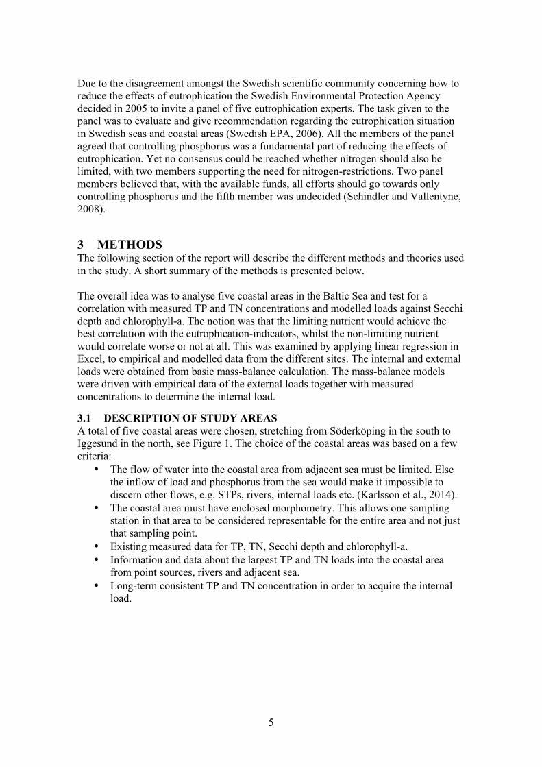
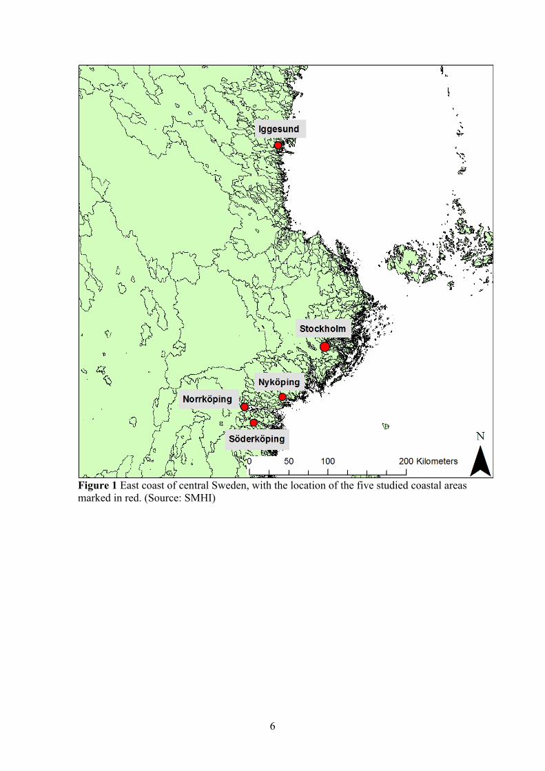
3.1 DESCRIPTION OF STUDY AREAS A total of five coastal areas were chosen, stretching from Söderköping in the south to Iggesund in the north, see Figure 1. The choice of the coastal areas was based on a few criteria:

• The flow of water into the coastal area from adjacent sea must be limited. Else the inflow of load and phosphorus from the sea would make it impossible to discern other flows, e.g. STPs, rivers, internal loads etc. (Karlsson et al., 2014).

• The coastal area must have enclosed morphometry. This allows one sampling station in that area to be considered representable for the entire area and not just that sampling point.

• Existing measured data for TP, TN, Secchi depth and chlorophyll-a. • Information and data about the largest TP and TN loads into the coastal area

from point sources, rivers and adjacent sea. • Long-term consistent TP and TN concentration in order to acquire the internal

load.

6

Figure 1 East coast of central Sweden, with the location of the five studied coastal areas marked in red. (Source: SMHI)

7

The sites differed regarding their volume, area and max-depth, but the difference in salinity was rather small (Table 1). Normally the salinity gradient in the Baltic Sea ranges from almost freshwater in the Bothnian Sea (north) to almost full-strength seawater in Kattegat (south). The effect of the south-to-north gradient, according to the general theory, is phosphorus limitation to the north and nitrogen limitation to the south (Granéli, 1990). This north-to-south gradient could not be observed for the studied sites, a consequence of the enclosed morphometry and inflow of freshwater. Table 1 An overview of some morphometric characteristics of the different coastal areas and the salinity.

Study area Volume [km3]

Area [km2]

Max depth [m]

Salinity [PSU]

Gårdsfjärden-Iggesund 0.031 6.3 16 3.93 Stockholm inner

archipelago 1.45* 108* 57* 4.03

Bays of Nyköping 0.012 10.1 17** 3.48 Bråviken-Norrköping 0.79 103 35 3.76

Slätbaken-Söderköping 0.18 15.4 44 3.65

Reference (SMHI, 2003), (Karlsson et al.,

2014)*

(SMHI, 2003),

(Karlsson et al., 2014)*

(SMHI, 2003), (Karlsson et al.,

2014)*, From sampling data**

Calculated from sampling data

8

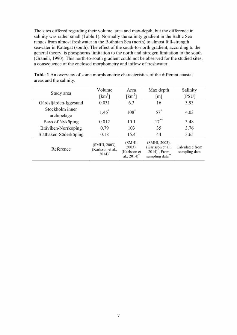
3.1.1 Gårdsfjärden The enclosed bay of Gårdsfjärden is situated just outside the town of Iggesund in the County of Gävleborg. Figure 2 shows were the sampling stations were located. K179 is the sampling station inside the bay and K190 is the reference station for the adjacent sea. Three of the primary sources of phosphorus and nitrogen into Gårdsfjärden were identified as:

• The inflow from river Delångersån (Lindgren, 2004). • The discharge water from a paper mill, Iggesund Mill (Lindgren, 2004). • Inflow from the adjacent sea.

Figure 2 The coastal area around Iggesund, with the sampling station of Gårdsfjärden (K179), the sampling station for the adjacent sea (K190) and outflow of Delångersån. (Source: SMHI)

9

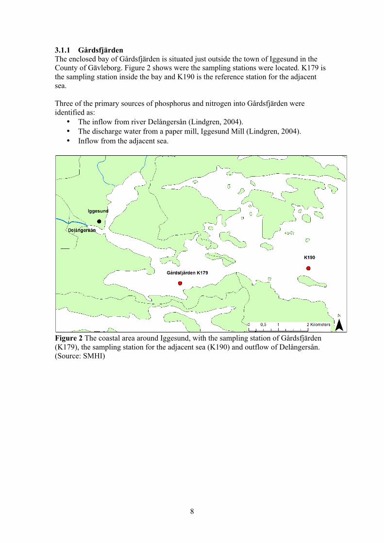
3.1.2 Stockholm’s inner archipelago Stockholm’s inner archipelago is situated in the middle of Stockholm city, with the city on all sides including on the islands. The archipelago is divided into several small bays, with varying morphometry and islands in between. The main exchange of water occurs via a narrow sound (Oxdjupet) (Lücke, 2016). The sampling stations used in this study are presented in Figure 3, with Trälhavet II as a reference station and the other five stations used to calculate the average concentrations in the entire archipelago. The concentration of TP and TN in Stockholm inner archipelago is primarily effected by the dynamics of three factors (Lücke, 2016)

• The inflow of fresh surface water from Lake Mälaren via river Norrström. • Three STPs: Bromma, Henriksdal and Käppala. • The inflow of salty bottom water from the outer archipelago via Oxsundet.

Figure 3 Stockholm’s inner archipelago with the sampling stations marked in red. The station Trälhavet II was the reference for the adjacent sea, while the other stations was used to calculate the concentrations. Also marked is the outflow of river Norrström. (Source: SMHI)

10

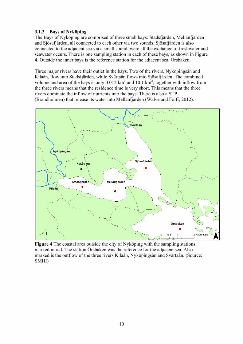
3.1.3 Bays of Nyköping The Bays of Nyköping are comprised of three small bays: Stadsfjärden, Mellanfjärden and Sjösafjärden, all connected to each other via two sounds. Sjösafjärden is also connected to the adjacent sea via a small sound, were all the exchange of freshwater and seawater occurs. There is one sampling station in each of these bays, as shown in Figure 4. Outside the inner bays is the reference station for the adjacent sea, Örsbaken. Three major rivers have their outlet in the bays. Two of the rivers, Nyköpingsån and Kilaån, flow into Stadsfjärden, while Svärtaån flows into Sjösafjärden. The combined volume and area of the bays is only 0.012 km3 and 10.1 km2, together with inflow from the three rivers means that the residence time is very short. This means that the three rivers dominate the inflow of nutrients into the bays. There is also a STP (Brandholmen) that release its water into Mellanfjärden (Walve and Folff, 2012).

Figure 4 The coastal area outside the city of Nyköping with the sampling stations marked in red. The station Örsbaken was the reference for the adjacent sea. Also marked is the outflow of the three rivers Kilaån, Nyköpingsån and Svärtaån. (Source: SMHI)

11

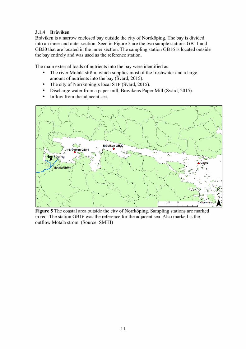
3.1.4 Bråviken Bråviken is a narrow enclosed bay outside the city of Norrköping. The bay is divided into an inner and outer section. Seen in Figure 5 are the two sample stations GB11 and GB20 that are located in the inner section. The sampling station GB16 is located outside the bay entirely and was used as the reference station. The main external loads of nutrients into the bay were identified as:

• The river Motala ström, which supplies most of the freshwater and a large amount of nutrients into the bay (Svärd, 2015).

• The city of Norrköping’s local STP (Svärd, 2015). • Discharge water from a paper mill, Bravikens Paper Mill (Svärd, 2015). • Inflow from the adjacent sea.

Figure 5 The coastal area outside the city of Norrköping. Sampling stations are marked in red. The station GB16 was the reference for the adjacent sea. Also marked is the outflow Motala ström. (Source: SMHI)

12

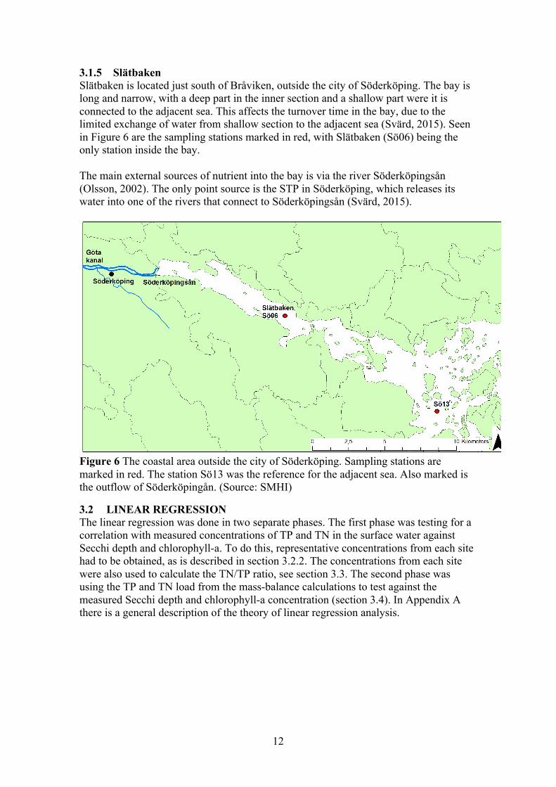
3.1.5 Slätbaken Slätbaken is located just south of Bråviken, outside the city of Söderköping. The bay is long and narrow, with a deep part in the inner section and a shallow part were it is connected to the adjacent sea. This affects the turnover time in the bay, due to the limited exchange of water from shallow section to the adjacent sea (Svärd, 2015). Seen in Figure 6 are the sampling stations marked in red, with Slätbaken (Sö06) being the only station inside the bay. The main external sources of nutrient into the bay is via the river Söderköpingsån (Olsson, 2002). The only point source is the STP in Söderköping, which releases its water into one of the rivers that connect to Söderköpingsån (Svärd, 2015).

Figure 6 The coastal area outside the city of Söderköping. Sampling stations are marked in red. The station Sö13 was the reference for the adjacent sea. Also marked is the outflow of Söderköpingån. (Source: SMHI)

3.2 LINEAR REGRESSION The linear regression was done in two separate phases. The first phase was testing for a correlation with measured concentrations of TP and TN in the surface water against Secchi depth and chlorophyll-a. To do this, representative concentrations from each site had to be obtained, as is described in section 3.2.2. The concentrations from each site were also used to calculate the TN/TP ratio, see section 3.3. The second phase was using the TP and TN load from the mass-balance calculations to test against the measured Secchi depth and chlorophyll-a concentration (section 3.4). In Appendix A there is a general description of the theory of linear regression analysis.

13

3.2.1 Theory and variables The reason for using linear regression with the concentration of TP and TN was the assumption that there would be a somewhat linear relationship between the concentrations and the primary production indicators. The indicators were:

• Chlorophyll-a, which is a measurement of the phytoplankton’s biomass (HELCOM, 2009).

• Secchi depth, an indicator of water transparency and a symptom of eutrophication (HELCOM, 2009).

A linear relationship was expected due to the fact that TP and TN include all the phosphorous and nitrogen in the water, which includes both inorganically and organically forms. Both nitrogen and phosphorus are essential nutrients for primary production, but only the mineral forms can be taken up by algae (Håkanson and Bryhn, 2008). So by definition, both TP and TN is partially a measurement of the level of biomass. A consequence of this is that the TP and TN concentration often match each other (Walve and Rolff, 2016) Due to the hypothesis that either phosphorous or nitrogen would be limiting, it was expected that when the inorganic form of the limiting nutrient was exhausted, and the system was limited by either nutrient, the concentration of TP or TN would directly correspond with the amount of phytoplankton in the water. Therefore there would be a linear relationship between Secchi depth and chlorophyll-a and the concentration of the limiting nutrient. Routinely both the mineral form of nitrogen and phosphorus are measured together with TP and TN. To determine the long-term limiting nutrient the TP and TN concentration was chosen for two reasons. Firstly, the difficulty in accurately measuring mineral nitrogen and phosphorus inherently leads to unreliable data (Håkanson et al., 2007). Secondly, the amount mineral form changes rapidly, in the order of seconds and days. Therefore using the measured mineral form, to determine the limiting nutrient, is best suited for a short time-scale (Håkanson et al., 2007; Ptacnik et al., 2010). Both Secchi depth and chlorophyll-a are influenced by other factors than nitrogen and phosphorus. Chlorophyll-a is a measurement of the amount of phytoplankton biomass, which is profoundly influence by the temperature and light condition. In the winter months this variable can be expected to be low, regardless of the amount of nitrogen and phosphorus. Secchi depth is a measurement of the water clarity and is mainly affected by three factors (Håkanson and Bryhn, 2008):

• The amount primary production in the system; more phytoplankton means lower Secchi depth.

• Materials from rivers and runoff from land. • Resuspended materials via wind and wave activity, together with land uplift.

The method of using linear regression to test for the limiting nutrient was tried in the experiment in Himmerfjärden (Elmgren and Larsson, 1997). The variables tested were the yearly average of TP and TN concentrations (upper 0–10 meters) with the summer average of chlorophyll-a. Only TN was found to have a clear correlation with chlorophyll-a, which indicated nitrogen limitation. In the experiment several other methods were used to determine the limiting nutrient.

14

All methods demonstrated the same general result, that nitrogen was the limiting nutrient, giving credibility to the method of using linear regression. However the method could not account for periodic phosphorus limitations, it could only suggest which nutrient was limiting during most years. Håkanson and Bryhn (2008) describe several models to predict the concentration of chlorophyll-a and Secchi depth. The models contain measured concentrations of TP and TN in the surface water during the summer months (May–September). Using concentrations sampled during the summer months minimizes the impact that other limiting variables could have on phytoplankton production, such as sunlight and temperature.

3.2.2 Data from sampling stations To be able to implement the regression analyses the data had to be organized based on which stations, what sampling depth and yearly time period to use. The sampling programs for the coastal areas varied greatly between sites. Furthermore the individual sampling programs differed both in sampling frequency and extent, which made the data heterogeneously distributed.

The method used for each studied site consequently differs slightly between sites and was modified, based on the available data, to get representative concentrations.

For all the studied coastal areas, except Iggesund and Slätbaken, there were data from several sampling stations. In those sites an average was calculated from the all stations that met two criteria:

• The sampling station was not allowed to be located directly at a river-outlet, STP or the adjacent sea.

• Stations only sampled sporadically during the studied time period were excluded.

The definition of surface water was based on the study by Elmgren and Larsson (1997), were they used the average concentration in the upper 0–10 meters to represent the concentration in the surface water. However in this study most of the sites sampling programs only entailed continuous measurement at 0.5 meter (Table 2). Therefore an average over time from 0.5 meters was calculated for all sites and tested in the linear regression analyses. Additionally for the stations that had sampling data from 0–10 meters, an average both over depth and through time, was calculated and tested in the linear regression analyses. The effect of using an average concentration from only 0.5 meter depth, instead of 0–10 meters, was tested for in Gårdsfjärden (Appendix B). The sampling-period for the different variables varied between sites. Most commonly concentrations of TP and TN, together with Secchi depth, had been sampled since the mid 1970s or early 80s. Chlorophyll-a was sporadically measured, with gaps of several years and in some cases only measured once a year. In Table 2 summarises the sampling programs.

15

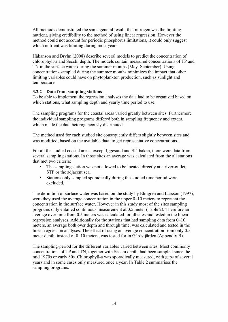
Table 2 Summary of the monitoring programs for the different sites: the sampling period for each variable, the continuous sampling depth, number of sampling stations and the reference of the data.

Gårdsfjärden Stockholm Nyköping Bråviken Slätbaken

TP and TN 1980–2015 1982–2015 1980–2016 1975–2016 1975–2014

Secchi depth 1980–2015 1982–2015 1980–2016* 1975–2016 1975–2014

Chl-a 1980–2015* 1982–2015 1996–2016** 1999–2016* 1993–2014

Sampl. depth 0.5–10 m 0.5–8 m 0.5 m 0.5m 0.5 m

Nr. of stations 1 5 3 2 1

Reference Lundgren, pers. Stockholm

vatten, pers. Nydahl, pers. Melander, pers. Melander, pers.

Not measured *1981, 85, 94

and 2011

*2000 **1998–2000

*2011

The choice of time period for the regression analyses was an iterative process. The starting point was using yearly averages for the period May to September to find a correlation. The same periods used in Elmgren and Larsson (1997) and Håkansson and Bryhn (2008).This was done for each variable. Then by plotting “scatterplots” and a trendline in Excel, the time period with the best correlation was chosen and tested for statistical significance. If no correlation could be found with the two time periods, the next time period was based on sampling-schedule in that specific area. The only site in which this had to be implemented was Slätbaken, where the sampling-schedule caused that the season April–October to also be tested. Only the time period with the best correlation was presented in the result.

3.3 REDFIELD RATIO The Redfield ratio represents the average composition of algae (C106N16P). The ratio of 16 atoms of nitrogen and one phosphorus expresses in what quantity the different nutrient are necessary for algae to develop (Redfield, 1958). It has been commonly used to describe the long-term limiting nutrient in aquatic-ecosystem (Swedish EPA, 2006; Håkanson and Bryhn, 2008; HELCOM 2009; Ptacnik et al., 2010). By weight the Redfield ratio is 7.2 and a lower TN/TP ratio indicate that the system is nitrogen limited and the conditions are favourable for N2-fixatiing cyanobacteria. Empirical data have shown that the threshold ratio for N2-fixatiing cyanobacteria is actually closer to 15 (Håkanson et al., 2007). If the TN/TP is higher than 7.2 it indicates that the system is phosphorous limited. The Redfield ratio was calculated for the same summer-period as that used in the linear regression analyses. The intent was to use the ratio as an indicator of the limiting nutrient. But as shown in Ptacnik et al. (2010) the TN/TP ratio is often an inadequate variable to determine the limiting nutrient, at least on a short time-scale.

16

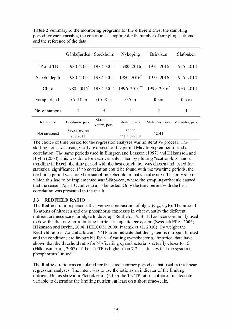
3.4 MODEL To get an understanding of the environmental conditions in each of the sites, mass-balance calculations were performed. These budget calculations allowed for quantification of nutrient fluxes within the areas and how they changed over the years. Not only did this provide the external load, but also of the internal load of nutrients. Mass-balance models have been used since the 1960s to predict eutrophication levels in lakes. The first was developed by Richard Vollenweider in 1965 and was based on the assumption that lakes are limited by phosphorus. Using basic hydrological, morphometric, and phosphorus loading data of the lake, the model could predict phosphorus concentration and the thereby the lakes eutrophic state (Brown and Simpson, 2001). The Vollenweider model was not used in this study, but its basic set up for calculating the mass balance with hydrological, morphometric, and loading data was. The general model was based on using time-series of the concentrations of TN and TP together with the respective water flow from the major point sources, rivers and the adjacent sea (Figure 7). These main external loads were used as dynamic inputs in the model. Allowing the modelled surface concentration to change based on the external loads. As there are also internal loads of TN and TP a calibration step was necessary (see section 3.4.6). This next step utilized measured concentrations in the surface water to calibrate the model, with two dynamic input and output variables, thus optimizing the simulated surface water to match that of the measured one. This provided the internal load of nutrients. Each modelled system was treated as a one-box system, were the surface concentration was set as the concentration in the entire box. The software Stella® was used to numerically solve the ordinary differential equations that the model entailed.

Figure 7 Schematic view of the mass-balance model. Internal loading is regulated through the input and output boxes at the bottom.

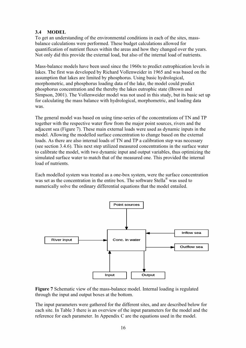
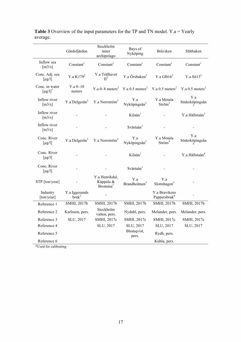
The input parameters were gathered for the different sites, and are described below for each site. In Table 3 there is an overview of the input parameters for the model and the reference for each parameter. In Appendix C are the equations used in the model.

17

Table 3 Overview of the input parameters for the TP and TN model. Y.a = Yearly average.

Gårdsfjärden Stockholm

inner archipelago

Bays of Nyköping Bråviken Slätbaken

Inflow sea [m3/s] Constant1 Constant1 Constant1 Constant1 Constant1

Conc. Adj. sea [µg/l] Y.a K1792 Y.a Trälhavet

II2 Y.a Örsbaken2 Y.a GB162 Y.a Sö132

Conc. in water [µg/l]*

Y.a 0–10 meters Y.a 0–8 meters2 Y.a 0.5 meters2 Y.a 0.5 meters2 Y.a 0.5 meters2

Inflow river [m3/s] Y.a Delgerån2 Y.a Norrström3 Y.a

Nyköpingsån3 Y.a Motala

Ström3

Y.a Söderköpingsån

3 Inflow river

[m3/s] - - Kilaån1 - Y.a Hällstaån3

Inflow river [m3/s] - - Svärtaån1 - -

Conc. River [µg/l] Y.a Delgerån3 Y.a Norrström4 Y.a

Nyköpingsån3 Y.a Motala

Ström4

Y.a Söderköpingsån

4

Conc. River [µg/l] - - Kilaån1 - Y.a Hällstaån4

Conc. River [µg/l] - - Svärtaån1 - -

STP [ton/year] - Y.a Henrikdal,

Käppala & Bromma2

Y.a Brandholmen5

Y.a Slottshagen5 -

Industry [ton/year]

Y.a Iggesunds bruk2 -

Y.a Bravikens Pappersbruk6 -

Reference 1 SMHI, 2017b SMHI, 2017b SMHI, 2017b SMHI, 2017b SMHI, 2017b

Reference 2 Karlsson, pers. Stockholm vatten, pers. Nydahl, pers. Melander, pers. Melander, pers.

Reference 3 SLU, 2017 SMHI, 2017c SMHI, 2017c SMHI, 2017c SMHI, 2017c Reference 4 SLU, 2017 SLU, 2017 SLU, 2017 SLU, 2017

Reference 5 Blomqvist,

pers. Rydh, pers. Reference 6 Kuhla, pers.

*Used for calibrating

18

3.4.1 Gårdsfjärden The mass-balance calculations for Gårdsfjärden were based on three main sources of TP and TN. These were the external load from Delgerån (river), a paper mill and the inflow from the adjacent sea. The models were run on a yearly time-basis and adjusted to fit the yearly average of measured concentrations in the top 0–10 meters of surface water.

3.4.2 Stockholm’s inner archipelago The mass-balance calculations for Stockholm inner archipelago were based on three main sources of TP and TN. These were the load from river Norrström, the STPs and the inflow from the adjacent sea. The models were run on a yearly time-basis and adjusted to fit the yearly average measured concentrations in the top 0–8 meters of surface water.

3.4.3 Bays of Nyköping The mass-balance calculations for the Bays of Nyköping were based on three main sources of TP and TN. These were the inflow from three rivers, STPs and the inflow from the adjacent sea. The models were run on a yearly time-basis and adjusted to fit the annual average in measured concentrations in the top 0.5 meters of surface water.

3.4.4 Bråviken The mass-balance calculations for Bråviken were based on four main sources of TP and TN. These were the load from the river Motala Ström, the STP, Braviken paper industry and the inflow from the adjacent sea. The models were run on a yearly time-basis and adjusted to fit the annual average measured concentrations in the top 0.5 meters of surface water.

3.4.5 Slätbaken The mass-balance calculations for Slätbaken were based on two main sources of TP and TN. These were the loads from the rivers and from the adjacent sea. The models were run on a yearly time-basis and adjusted to fit the annual average measured concentrations in the top 0.5 meters of surface water.

3.4.6 Model input parameters Though the idea was to use only empirical data in the model, not all parameters were sampled or available from monitoring programs. The missing parameters were the inflow from the adjacent sea and the waterflow from two rivers with outlets in the Bays of Nyköping. These gaps in the input-data were filled with data from Swedish Metrological and Hydrological Institutes (SMHIs) S-HYPE model. The S-HYPE model is a hydrological model that simulates flows, turnover time and water quality with a high spatial resolution for most coastal waters, rivers and lakes in Sweden (SMHI, 2017a) The model was run with two separate sets of data, one for TP and one for TN. The first model-run was done solely with the external loads. Euler’s method was employed in the program Stella® to interpolate and numerically solve the differential equations. From the interpolated results, the program summed up the total load from each year, providing the total external load from each year. The program also calculated the amount of nutrients in the system at a given year, which could be converted into concentrations. These modelled concentrations were then compared to the measured concentrations.

19

The difference between measured and modelled concentrations expressed the need for additional input or output of TP and TN, through which the model was calibrated. The equations used for the calibration of the model can be found in Appendix C. The biggest difference between the models were the two dynamic input and output factors and what they represented. Both factors were meant to depict the internal pool of nitrogen and phosphorus, which by themselves can be substantial loads (HELCOM, 2009). The principal processes that regulate the internal pool of nitrogen are N2-fixation by cyanobacteria, the release of N2 from bacteria-driven denitrification and to some extent by anammox (HELCOM, 2009). These processes enable the uptake or release of inorganic nitrogen gas to the internal pool of nitrogen, increasing or decreasing the amount of bio-available nitrogen. For phosphorus there are no microbial processes to increase or decrease the internal pool through uptake or release of a gaseous form. Instead, processes in the sediments mainly determine the internal pool of phosphorus. Phosphorus reserves, accumulated in the sediment, can be released back to the water during anoxic periods in the sediments (HELCOM, 2009). Mechanical processes, such as land uplift and erosion by wind and waves, also affect the internal load of phosphorus and nitrogen. Both nutrients can also be buried in the sediments, making them inaccessible for release (Granéli, 1990; Karlsson et al., 2014). The purpose of modelling the nutrient fluxes was not to ascertain the contribution of each internal process, but the sum of the internal loading. Consequently the input and output factors are presented as either internal loading, burial or in the case of nitrogen burial and denitrification. The obtained internal and external loads were then tested with the same linear regression tools as described in Appendix A. The sum of both the internal and external loads (total load), as well as a separate test with just the external, was done with the same values of Secchi depth and chlorophyll-a from the iterative process in section 3.2.1. The external load was tested separately from the total load, as not all sites had measured data of the concentrations in the upper 0–10 meters. Therefore the calibration and the subsequent internal loading in some of the sites were uncertain.

20

4 RESULTS The results are divided into different section for each studied site, starting with the northern most site of Gårdsfjärden and ending with the southernmost site of Slätbaken. The presented results are that of the linear regression analyses, TN/TP ratio, the modelled nutrient fluxes and the calculated TP and TN loading. There is also a section in the end, with a short summary of the results from all the sites.

4.1 GÅRDSFJÄRDEN

4.1.1 Linear regression analysis (conc.) and TN/TP ratio The linear regression analyses of data that attained the best correlation were based on the yearly average of concentrations and Secchi depths during the season May to September, from the period 1980–2014. The concentrations of TP, TN and chlorophyll-a were calculated from samples taken at 0.5 meters depth together with Secchi depth, from sampling station K179 in Gårdsfjärden. The linear regression analyses with the concentrations and modelled loads are presented in Table 4 and Table 5 respectively, with the r2-value of each trendline, the corresponding r-value and the p-value. The analyses of both TN and TP concentration together with Secchi depth achieved a significant negative trend (p<0.05). The highest correlation coefficient to describe the Secchi depth was with the TN concentration, with an r-value of –0.73. The regression analyses with TP concentration and Secchi depth and also gave a significant trend and a correlation coefficient of -0.68. The analysis with both TP and TN concentration indicated a negative correlation with chlorophyll-a, with TN achieving a significant correlation. Its implication being that a higher concentration of TN led to a lower concentration of chlorophyll-a. Table 4 A compilation of the r2-value of the trendline, the correlation coefficient r and the p-value from the linear regression with concentrations. Marked in bold are the regression lines with p <0.05.

Conc. r2 of TP r of TP P-value r2 of TN r of TN P-value Secchi depth 0.46 –0.68 <0.0001 0.53 –0.73 <0.0001

Chl-a 0.09 –0.29 0.12 0.19 –0.44 0.02

21

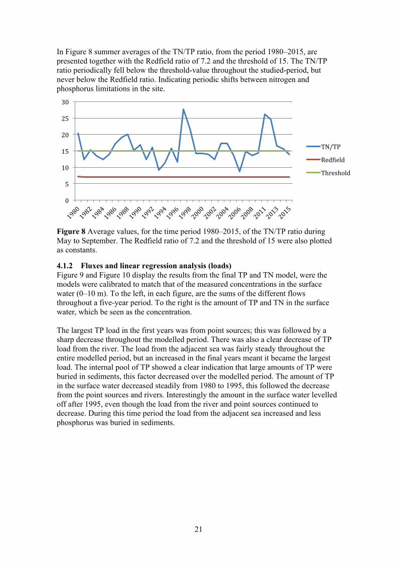
In Figure 8 summer averages of the TN/TP ratio, from the period 1980–2015, are presented together with the Redfield ratio of 7.2 and the threshold of 15. The TN/TP ratio periodically fell below the threshold-value throughout the studied-period, but never below the Redfield ratio. Indicating periodic shifts between nitrogen and phosphorus limitations in the site.

Figure 8 Average values, for the time period 1980–2015, of the TN/TP ratio during May to September. The Redfield ratio of 7.2 and the threshold of 15 were also plotted as constants.

4.1.2 Fluxes and linear regression analysis (loads) Figure 9 and Figure 10 display the results from the final TP and TN model, were the models were calibrated to match that of the measured concentrations in the surface water (0–10 m). To the left, in each figure, are the sums of the different flows throughout a five-year period. To the right is the amount of TP and TN in the surface water, which be seen as the concentration. The largest TP load in the first years was from point sources; this was followed by a sharp decrease throughout the modelled period. There was also a clear decrease of TP load from the river. The load from the adjacent sea was fairly steady throughout the entire modelled period, but an increased in the final years meant it became the largest load. The internal pool of TP showed a clear indication that large amounts of TP were buried in sediments, this factor decreased over the modelled period. The amount of TP in the surface water decreased steadily from 1980 to 1995, this followed the decrease from the point sources and rivers. Interestingly the amount in the surface water levelled off after 1995, even though the load from the river and point sources continued to decrease. During this time period the load from the adjacent sea increased and less phosphorus was buried in sediments.

0

5

10

15

20

25

30

TN/TPRed.ieldThreshold

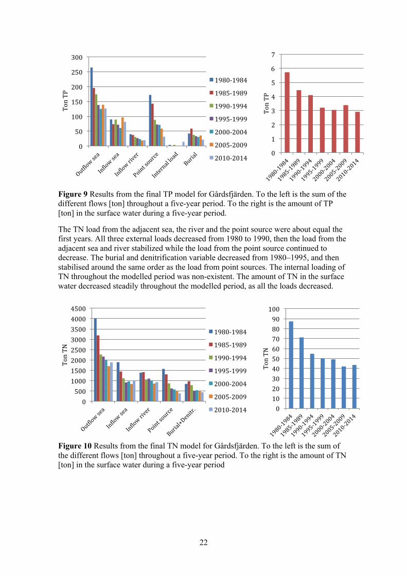
22

Figure 9 Results from the final TP model for Gårdsfjärden. To the left is the sum of the different flows [ton] throughout a five-year period. To the right is the amount of TP [ton] in the surface water during a five-year period.

The TN load from the adjacent sea, the river and the point source were about equal the first years. All three external loads decreased from 1980 to 1990, then the load from the adjacent sea and river stabilized while the load from the point source continued to decrease. The burial and denitrification variable decreased from 1980–1995, and then stabilised around the same order as the load from point sources. The internal loading of TN throughout the modelled period was non-existent. The amount of TN in the surface water decreased steadily throughout the modelled period, as all the loads decreased.

Figure 10 Results from the final TN model for Gårdsfjärden. To the left is the sum of the different flows [ton] throughout a five-year period. To the right is the amount of TN [ton] in the surface water during a five-year period

0

1

2

3

4

5

6

7

TonT

P

0

50

100

150

200

250

300TonTP

1980-19841985-19891990-19941995-19992000-20042005-20092010-2014

050010001500200025003000350040004500

TonT

N

1980-19841985-19891990-19941995-19992000-20042005-20092010-2014 0

102030405060708090100

TonT

N

23

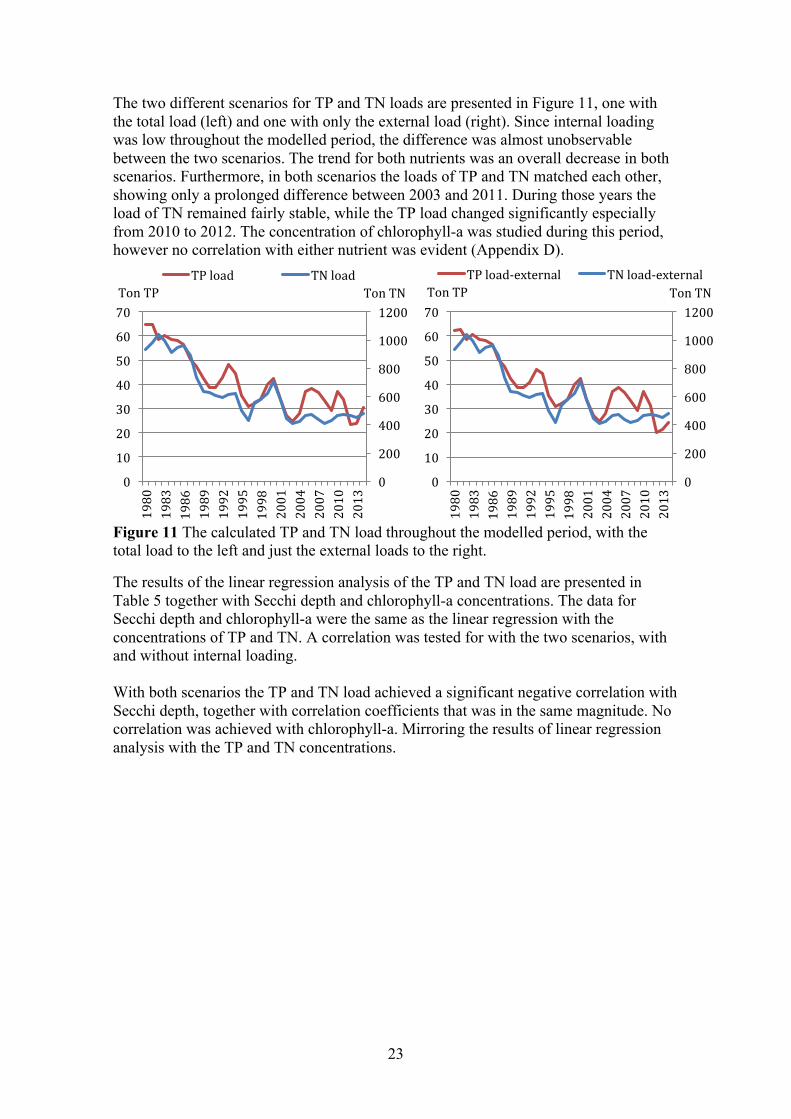
The two different scenarios for TP and TN loads are presented in Figure 11, one with the total load (left) and one with only the external load (right). Since internal loading was low throughout the modelled period, the difference was almost unobservable between the two scenarios. The trend for both nutrients was an overall decrease in both scenarios. Furthermore, in both scenarios the loads of TP and TN matched each other, showing only a prolonged difference between 2003 and 2011. During those years the load of TN remained fairly stable, while the TP load changed significantly especially from 2010 to 2012. The concentration of chlorophyll-a was studied during this period, however no correlation with either nutrient was evident (Appendix D).

Figure 11 The calculated TP and TN load throughout the modelled period, with the total load to the left and just the external loads to the right.

The results of the linear regression analysis of the TP and TN load are presented in Table 5 together with Secchi depth and chlorophyll-a concentrations. The data for Secchi depth and chlorophyll-a were the same as the linear regression with the concentrations of TP and TN. A correlation was tested for with the two scenarios, with and without internal loading. With both scenarios the TP and TN load achieved a significant negative correlation with Secchi depth, together with correlation coefficients that was in the same magnitude. No correlation was achieved with chlorophyll-a. Mirroring the results of linear regression analysis with the TP and TN concentrations.

0

200

400

600

800

1000

1200

010203040506070

1980

1983

1986

1989

1992

1995

1998

2001

2004

2007

2010

2013

TonTNTonTPTPload TNload

0

200

400

600

800

1000

1200

010203040506070

1980

1983

1986

1989

1992

1995

1998

2001

2004

2007

2010

2013

TonTNTonTPTPload-external TNload-external

24

Table 5 A compilation of the r2-value of the trendline, the correlation coefficient r and the p-value from the linear regression analyses. Two scenarios were used for the independent variables of TP and TN loads, one scenario with the total load and one with just the external load. Marked in bold are the regression lines with p <0,05

Total load r2 of TP r of TP P-value r2 of TN r of TN P-value

Secchi depth 0.52 –0.72 <0.0001 0.501 –0.71 <0.0001 Chl-a 0.12 –0.35 0.07 0.11 –0.33 0.08

External load r2 of TP r of TP P-value r2 of TN r of TN P-value

Secchi depth 0.58 –0.76 <0.0001 0.5 –0.71 <0.0001 Chl-a 0.11 +0.33 0.08 0.1 +0.32 0.09

4.2 STOCKHOLM

4.2.1 Linear regression analysis (conc.) and TN/TP ratio The linear regression analyses of data, that attained the best correlation, were based on the yearly average of concentrations and Secchi depths during the season May to September, from the period 1982–2015. The concentrations of TP, TN and chlorophyll-a were calculated from samples taken at 0.5 meters depth together with Secchi depth, at the sampling stations Kovikksudde, Karantänbojen, Halvkakssundet, Blockhusudde and Blomskär. The linear regression analyses with the concentrations and modelled loads are presented in Table 6 and Table 7 with the r2-value of each trendline, the corresponding r-value and the p-value. The regression analyses of both TP and TN concentration together with Secchi depth achieved a significant negative trend (p<0.05). The strongest correlation coefficient to describe the Secchi depth was with the TN concentration, with an r-value of –0.66. The regression analyses with TP concentration and Secchi depth also got a significant trend with a slightly lower correlation coefficient of –0.53. Both the TP and TN concentration together with chlorophyll-a achieved a significant positive correlation. The strongest correlation coefficient for chlorophyll-a was with the TP concentration, with an r-value of +0.65. The correlation coefficient for TN concentration and chlorophyll-a was +0.41. Table 6 A compilation of the r2-value of the trendline, the correlation coefficient r and the p-value from the linear regression analyses. Marked in bold are the regression lines with p <0.05.

Concentration r2 of TP r of TP P-value r2 of TN r of TN P-value

Secchi depth 0.28 –0.53 0.001 0.44 –0.66 <0.0001 Chl-a 0.42 +0.65 <0.0001 0.17 +0.41 0.002

25

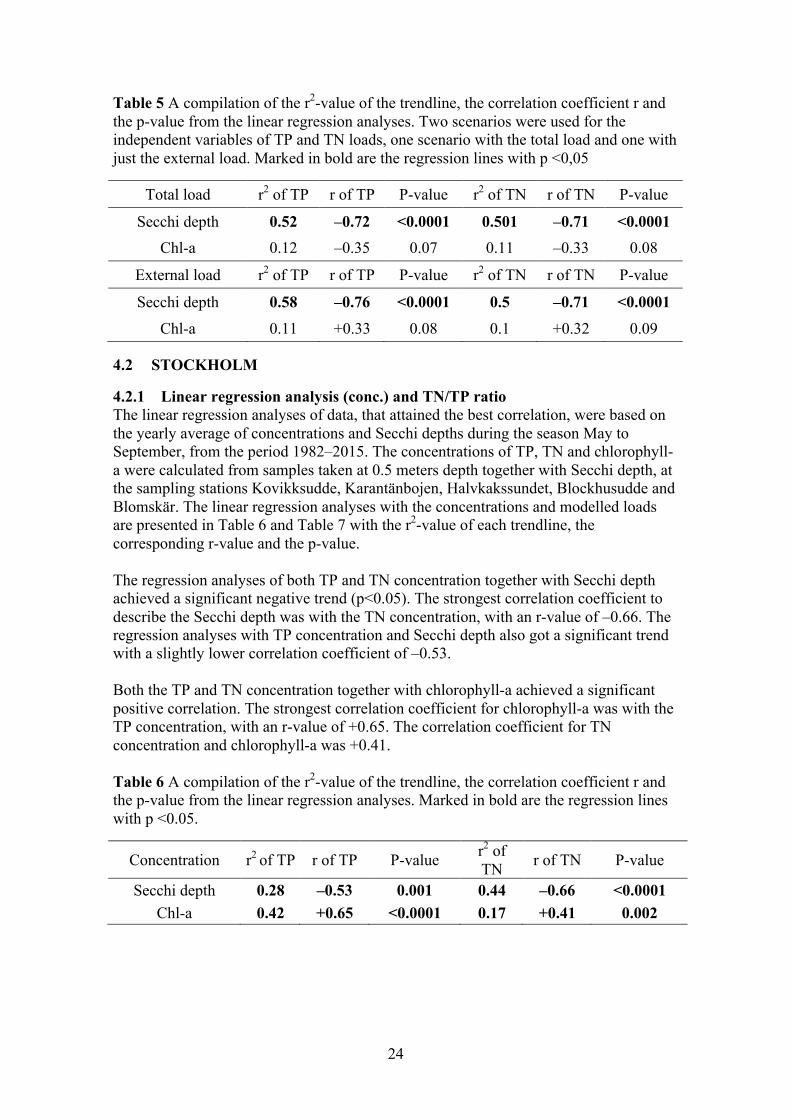
In Figure 12 summer averages of the TN/TP, from the period 1982 to 2015, are presented together with the Redfield ratio of 7.2 and the threshold of 15. The TN/TP ratio stayed continuously above the threshold value for the entire period, indicating long-term phosphorus-limitation.


4.2.2 Fluxes and linear regression analysis (loads) Figure 13 and Figure 14 display the results from the final TP and TN model, were the models were calibrated to match that of the measured concentrations in the surface water (0–8 m). To the left, in each figure, are the sums of the different flows throughout a five-year period. To the right is the amount of TP and TN in the surface water, which can also be seen as the concentration. The largest TP load was from the adjacent sea and it stayed steady throughout the modelled period. The load from the river was the second largest source of external TP, and this also stayed fairly stable. There was a small decrease of TP load from the STPs during 1990–1995, after that it levelled off. This decrease was observed in the amount of TP in the surface water, though it continued to decrease. Internal loading was only observable throughout the first years, 1990–1999. The burial factor was observable throughout the entire modelled period and there was a clear increase throughout the modelled period. The decrease in the amount of TP in the surface water correspondingly followed this trend.

0

5

10

15

20

25

30

35

40

1982

1984

1986

1988

1990

1992

1994

1996

1998

2000

2002

2004

2006

2008

2010

2012

2014


26

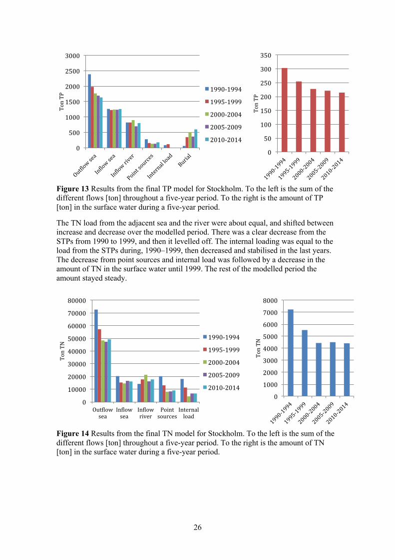
Figure 13 Results from the final TP model for Stockholm. To the left is the sum of the different flows [ton] throughout a five-year period. To the right is the amount of TP [ton] in the surface water during a five-year period.

The TN load from the adjacent sea and the river were about equal, and shifted between increase and decrease over the modelled period. There was a clear decrease from the STPs from 1990 to 1999, and then it levelled off. The internal loading was equal to the load from the STPs during, 1990–1999, then decreased and stabilised in the last years. The decrease from point sources and internal load was followed by a decrease in the amount of TN in the surface water until 1999. The rest of the modelled period the amount stayed steady.

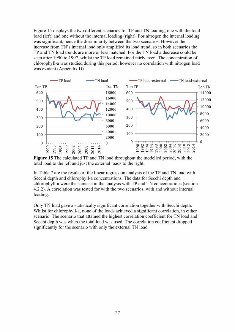
Figure 14 Results from the final TN model for Stockholm. To the left is the sum of the different flows [ton] throughout a five-year period. To the right is the amount of TN [ton] in the surface water during a five-year period.

0

500

1000

1500

2000

2500

3000TonT

P 1990-19941995-19992000-20042005-20092010-2014

0

50

100

150

200

250

300

350

TonT

P

01000020000300004000050000600007000080000

Out.lowsea

In.lowsea

In.lowriver

Pointsources

Internalload

TonT

N

1990-19941995-19992000-20042005-20092010-2014

010002000300040005000600070008000

TonT

N

27

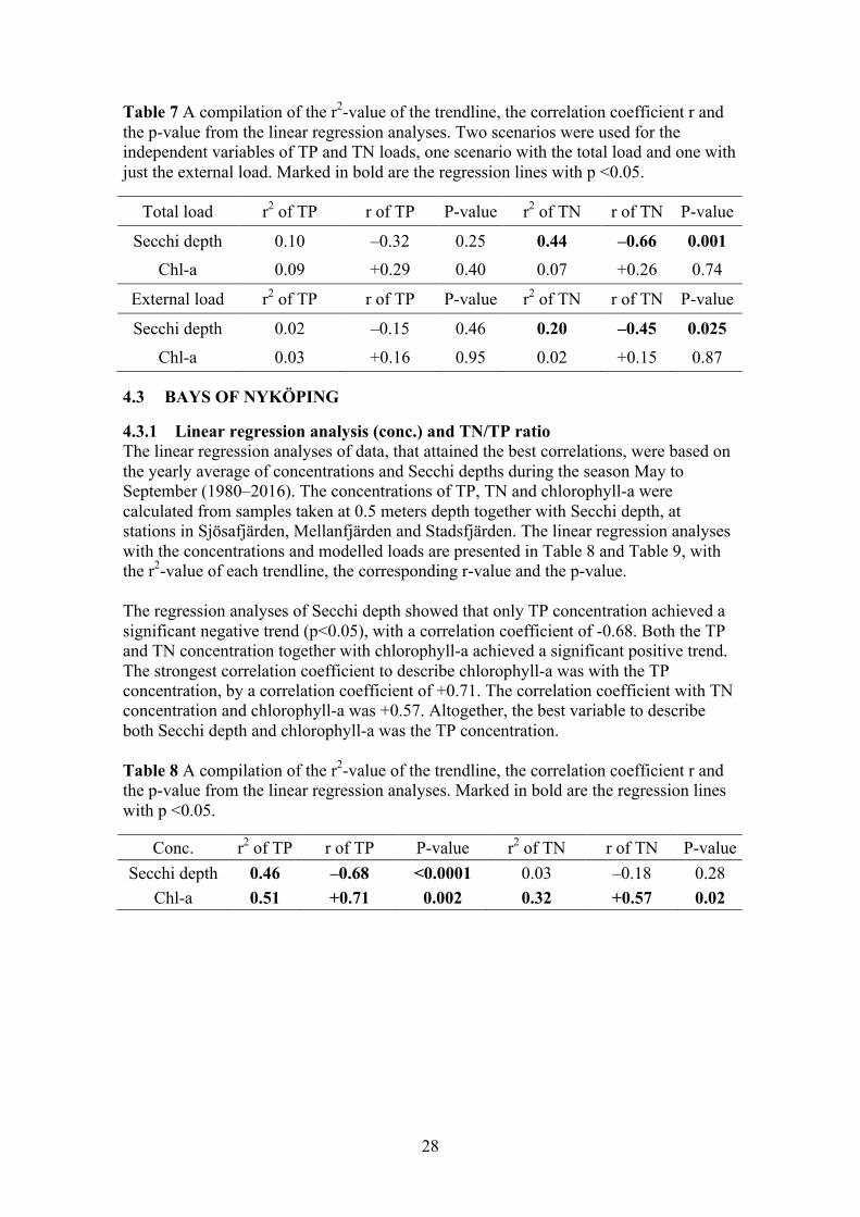
Figure 15 displays the two different scenarios for TP and TN loading, one with the total load (left) and one without the internal loading (right). For nitrogen the internal loading was significant, hence the dissimilarity between the two scenarios. However the increase from TN’s internal load only amplified its load trend, so in both scenarios the TP and TN load trends are more or less matched. For the TN load a decrease could be seen after 1990 to 1997, whilst the TP load remained fairly even. The concentration of chlorophyll-a was studied during this period, however no correlation with nitrogen load was evident (Appendix D).


In Table 7 are the results of the linear regression analysis of the TP and TN load with Secchi depth and chlorophyll-a concentrations. The data for Secchi depth and chlorophyll-a were the same as in the analysis with TP and TN concentrations (section 4.2.2). A correlation was tested for with the two scenarios, with and without internal loading. Only TN load gave a statistically significant correlation together with Secchi depth. Whilst for chlorophyll-a, none of the loads achieved a significant correlation, in either scenario. The scenario that attained the highest correlation coefficient for TN load and Secchi depth was when the total load was used. The correlation coefficient dropped significantly for the scenario with only the external TN load.

020004000600080001000012000140001600018000

0

100

200

300

400

500

600

1990

1993

1996

1999

2002

2005

2008

2011

2014


02000400060008000100001200014000

0

100

200

300

400

500

600

1990

1992

1994

1996

1998

2000

2002

2004

2006

2008

2010

2012

2014


28

Table 7 A compilation of the r2-value of the trendline, the correlation coefficient r and the p-value from the linear regression analyses. Two scenarios were used for the independent variables of TP and TN loads, one scenario with the total load and one with just the external load. Marked in bold are the regression lines with p <0.05.


Secchi depth 0.10 –0.32 0.25 0.44 –0.66 0.001 Chl-a 0.09 +0.29 0.40 0.07 +0.26 0.74



4.3 BAYS OF NYKÖPING

4.3.1 Linear regression analysis (conc.) and TN/TP ratio The linear regression analyses of data, that attained the best correlations, were based on the yearly average of concentrations and Secchi depths during the season May to September (1980–2016). The concentrations of TP, TN and chlorophyll-a were calculated from samples taken at 0.5 meters depth together with Secchi depth, at stations in Sjösafjärden, Mellanfjärden and Stadsfjärden. The linear regression analyses with the concentrations and modelled loads are presented in Table 8 and Table 9, with the r2-value of each trendline, the corresponding r-value and the p-value. The regression analyses of Secchi depth showed that only TP concentration achieved a significant negative trend (p<0.05), with a correlation coefficient of -0.68. Both the TP and TN concentration together with chlorophyll-a achieved a significant positive trend. The strongest correlation coefficient to describe chlorophyll-a was with the TP concentration, by a correlation coefficient of +0.71. The correlation coefficient with TN concentration and chlorophyll-a was +0.57. Altogether, the best variable to describe both Secchi depth and chlorophyll-a was the TP concentration. Table 8 A compilation of the r2-value of the trendline, the correlation coefficient r and the p-value from the linear regression analyses. Marked in bold are the regression lines with p <0.05.

Conc. r2 of TP r of TP P-value r2 of TN r of TN P-value Secchi depth 0.46 –0.68 <0.0001 0.03 –0.18 0.28

Chl-a 0.51 +0.71 0.002 0.32 +0.57 0.02

29

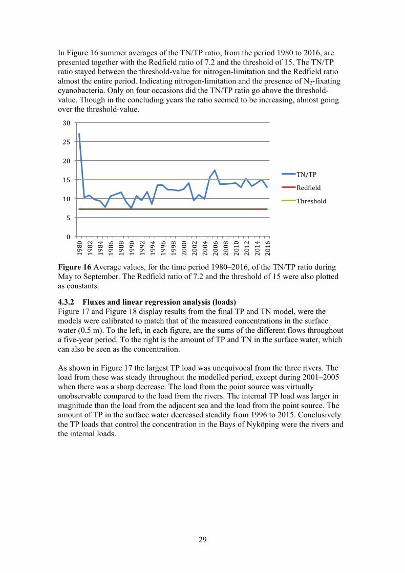
In Figure 16 summer averages of the TN/TP ratio, from the period 1980 to 2016, are presented together with the Redfield ratio of 7.2 and the threshold of 15. The TN/TP ratio stayed between the threshold-value for nitrogen-limitation and the Redfield ratio almost the entire period. Indicating nitrogen-limitation and the presence of N2-fixating cyanobacteria. Only on four occasions did the TN/TP ratio go above the threshold-value. Though in the concluding years the ratio seemed to be increasing, almost going over the threshold-value.


4.3.2 Fluxes and linear regression analysis (loads) Figure 17 and Figure 18 display results from the final TP and TN model, were the models were calibrated to match that of the measured concentrations in the surface water (0.5 m). To the left, in each figure, are the sums of the different flows throughout a five-year period. To the right is the amount of TP and TN in the surface water, which can also be seen as the concentration. As shown in Figure 17 the largest TP load was unequivocal from the three rivers. The load from these was steady throughout the modelled period, except during 2001–2005 when there was a sharp decrease. The load from the point source was virtually unobservable compared to the load from the rivers. The internal TP load was larger in magnitude than the load from the adjacent sea and the load from the point source. The amount of TP in the surface water decreased steadily from 1996 to 2015. Conclusively the TP loads that control the concentration in the Bays of Nyköping were the rivers and the internal loads.

0

5

10

15

20

25

30

1980

1982

1984

1986

1988

1990

1992

1994

1996

1998

2000

2002

2004

2006

2008

2010

2012

2014

2016


30

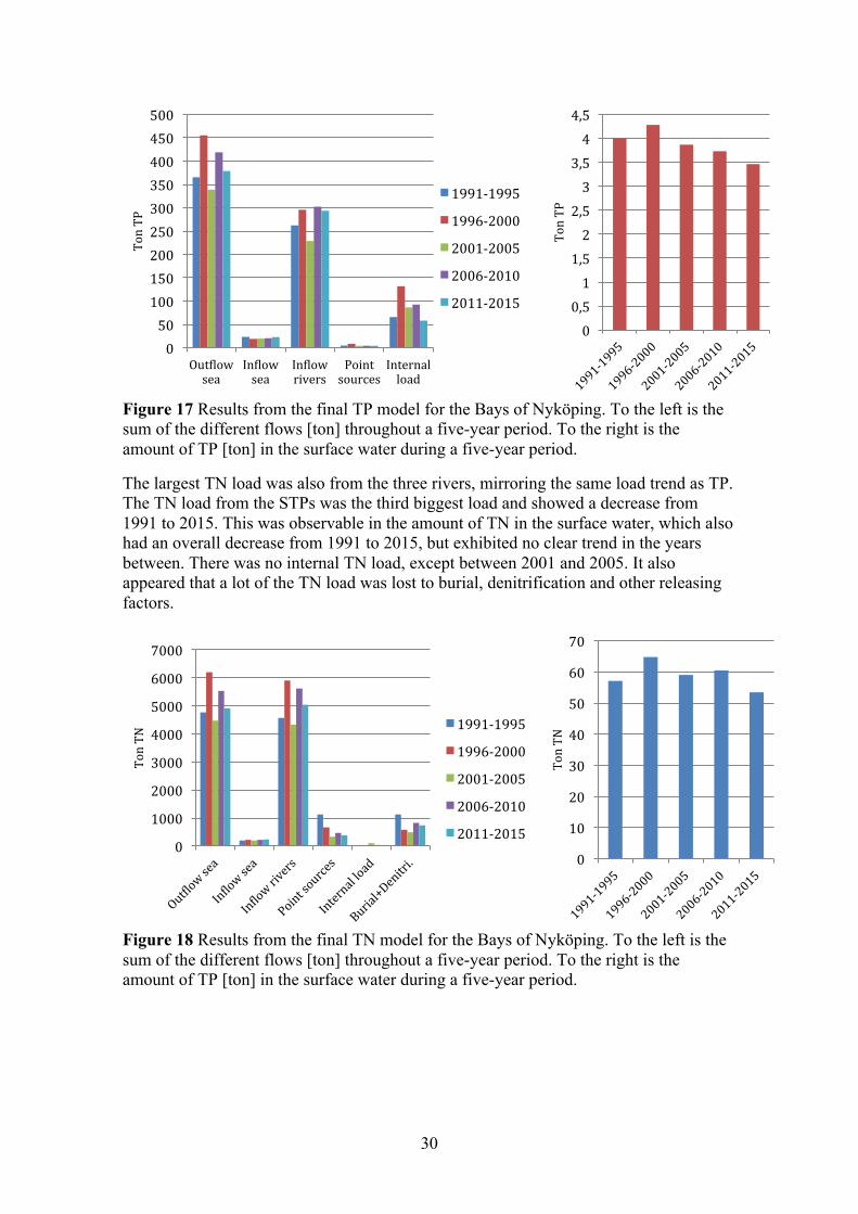
Figure 17 Results from the final TP model for the Bays of Nyköping. To the left is the sum of the different flows [ton] throughout a five-year period. To the right is the amount of TP [ton] in the surface water during a five-year period.

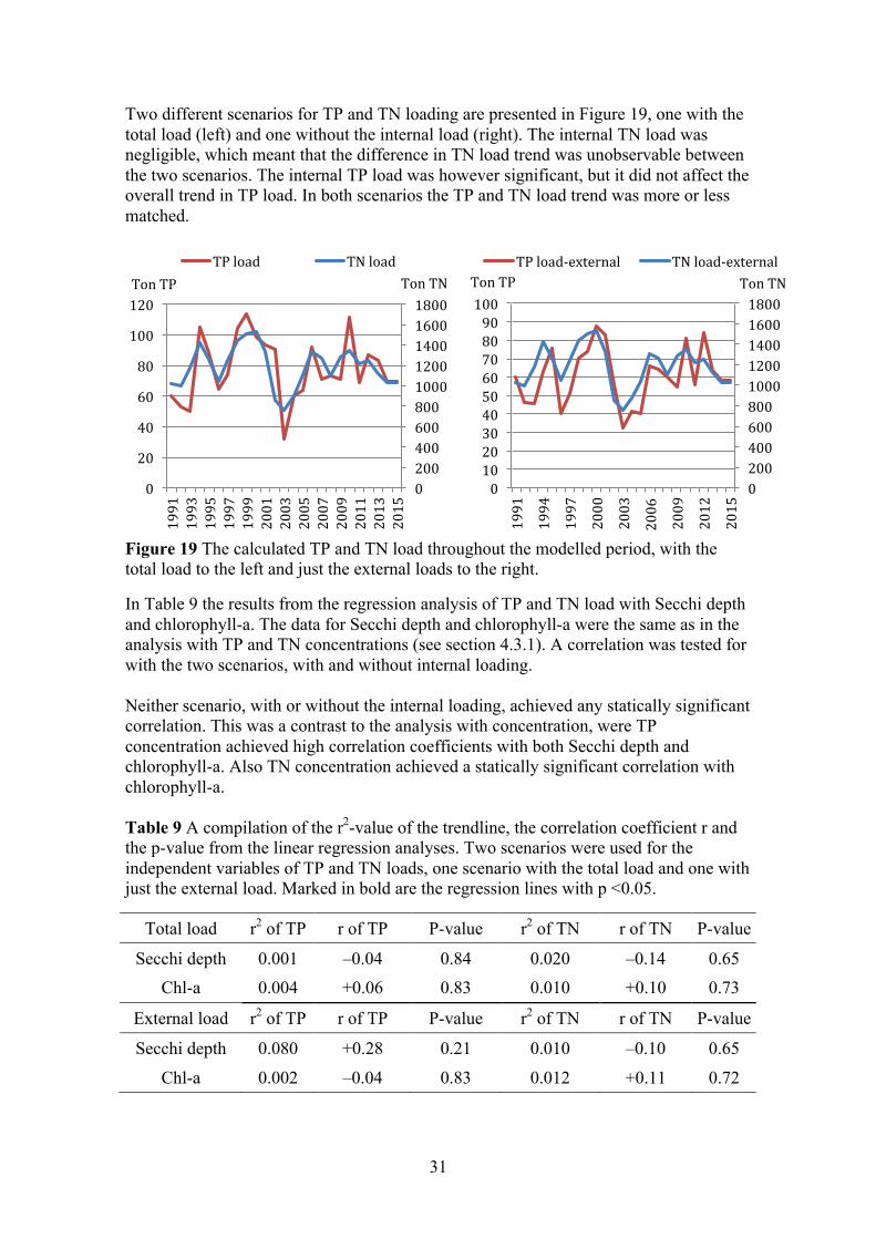
The largest TN load was also from the three rivers, mirroring the same load trend as TP. The TN load from the STPs was the third biggest load and showed a decrease from 1991 to 2015. This was observable in the amount of TN in the surface water, which also had an overall decrease from 1991 to 2015, but exhibited no clear trend in the years between. There was no internal TN load, except between 2001 and 2005. It also appeared that a lot of the TN load was lost to burial, denitrification and other releasing factors.

Figure 18 Results from the final TN model for the Bays of Nyköping. To the left is the sum of the different flows [ton] throughout a five-year period. To the right is the amount of TP [ton] in the surface water during a five-year period.

050100150200250300350400450500

Out.lowsea

In.lowsea

In.lowrivers

Pointsources

Internalload

TonT

P

1991-19951996-20002001-20052006-20102011-2015

00,51

1,52

2,53

3,54

4,5

TonT

P

01000200030004000500060007000

TonT

N 1991-19951996-20002001-20052006-20102011-2015

0

10

20

30

40

50

60

70

TonT

N

31

Two different scenarios for TP and TN loading are presented in Figure 19, one with the total load (left) and one without the internal load (right). The internal TN load was negligible, which meant that the difference in TN load trend was unobservable between the two scenarios. The internal TP load was however significant, but it did not affect the overall trend in TP load. In both scenarios the TP and TN load trend was more or less matched.


In Table 9 the results from the regression analysis of TP and TN load with Secchi depth and chlorophyll-a. The data for Secchi depth and chlorophyll-a were the same as in the analysis with TP and TN concentrations (see section 4.3.1). A correlation was tested for with the two scenarios, with and without internal loading. Neither scenario, with or without the internal loading, achieved any statically significant correlation. This was a contrast to the analysis with concentration, were TP concentration achieved high correlation coefficients with both Secchi depth and chlorophyll-a. Also TN concentration achieved a statically significant correlation with chlorophyll-a. Table 9 A compilation of the r2-value of the trendline, the correlation coefficient r and the p-value from the linear regression analyses. Two scenarios were used for the independent variables of TP and TN loads, one scenario with the total load and one with just the external load. Marked in bold are the regression lines with p <0.05.




Secchi depth 0.080 +0.28 0.21 0.010 –0.10 0.65

Chl-a 0.002 –0.04 0.83 0.012 +0.11 0.72

020040060080010001200140016001800

0

20

40

60

80

100

120

1991

1993

1995

1997

1999

2001

2003

2005

2007

2009

2011

2013

2015


020040060080010001200140016001800

0102030405060708090100

1991

1994

1997

2000

2003

2006

2009

2012

2015


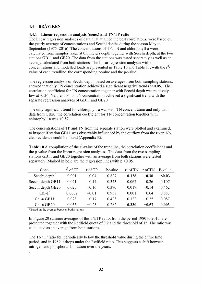
32

4.4 BRÅVIKEN

4.4.1 Linear regression analysis (conc.) and TN/TP ratio The linear regression analyses of data, that attained the best correlations, were based on the yearly average of concentrations and Secchi depths during the season May to September (1975–2016). The concentrations of TP, TN and chlorophyll-a were calculated from samples taken at 0.5 meters depth together with Secchi depth, at the two stations GB11 and GB20. The data from the stations was tested separately as well as an average calculated from both stations. The linear regression analyses with the concentrations and modelled loads are presented in Table 10 and Table 11, with the r2-value of each trendline, the corresponding r-value and the p-value. The regression analysis of Secchi depth, based on averages from both sampling stations, showed that only TN concentration achieved a significant negative trend (p<0.05). The correlation coefficient for TN concentration together with Secchi depth was relatively low at -0.36. Neither TP nor TN concentration achieved a significant trend with the separate regression analyses of GB11 and GB20. The only significant trend for chlorophyll-a was with TN concentration and only with data from GB20; the correlation coefficient for TN concentration together with chlorophyll-a was +0.57. The concentrations of TP and TN from the separate station were plotted and examined, to inspect if station GB11 was observably influenced by the outflow from the river. No clear evidence could be found (Appendix E). Table 10 A compilation of the r2-value of the trendline, the correlation coefficient r and the p-value from the linear regression analyses. The data from the two sampling stations GB11 and GB20 together with an average from both stations were tested separately. Marked in bold are the regression lines with p <0.05.

Conc. r2 of TP r of TP P-value r2 of TN r of TN P-value Secchi depth* 0.001 –0.04 0.827 0.128 –0.36 <0.03

Secchi depth GB11 0.021 –0.14 0.323 0.067 –0.26 0.107 Secchi depth GB20 0.025 –0.16 0.390 0.019 –0.14 0.462

Chl-a* 0.0002 –0.01 0.958 0.001 +0.04 0.883 Chl-a GB11 0.028 –0.17 0.423 0.122 +0.35 0.087 Chl-a GB20 0.055 +0.23 0.282 0.330 +0.57 0.003

*Based on the average between both stations In Figure 20 summer averages of the TN/TP ratio, from the period 1980 to 2015, are presented together with the Redfield quota of 7.2 and the threshold of 15. The ratio was calculated as an average from both stations. The TN/TP ratio fell periodically below the threshold value during the entire time period, and in 1989 it drops under the Redfield ratio. This suggests a shift between nitrogen and phosphorus limitation over the years. .

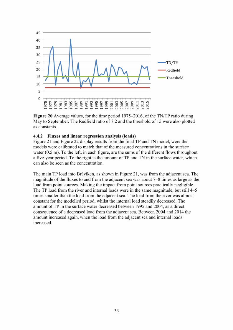
33


4.4.2 Fluxes and linear regression analysis (loads) Figure 21 and Figure 22 display results from the final TP and TN model, were the models were calibrated to match that of the measured concentrations in the surface water (0.5 m). To the left, in each figure, are the sums of the different flows throughout a five-year period. To the right is the amount of TP and TN in the surface water, which can also be seen as the concentration. The main TP load into Bråviken, as shown in Figure 21, was from the adjacent sea. The magnitude of the fluxes to and from the adjacent sea was about 7–8 times as large as the load from point sources. Making the impact from point sources practically negligible. The TP load from the river and internal loads were in the same magnitude, but still 4–5 times smaller than the load from the adjacent sea. The load from the river was almost constant for the modelled period, whilst the internal load steadily decreased. The amount of TP in the surface water decreased between 1995 and 2004, as a direct consequence of a decreased load from the adjacent sea. Between 2004 and 2014 the amount increased again, when the load from the adjacent sea and internal loads increased.

051015202530354045

1975

1977

1979

1981

1983

1985

1987

1989

1991

1993

1995

1997

1999

2001

2003

2005

2007

2009

2011

2013

2015


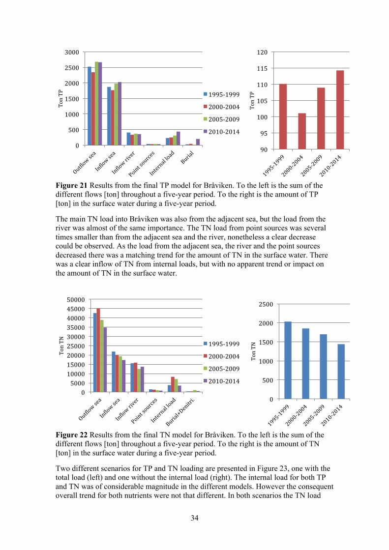
34

Figure 21 Results from the final TP model for Bråviken. To the left is the sum of the different flows [ton] throughout a five-year period. To the right is the amount of TP [ton] in the surface water during a five-year period.

The main TN load into Bråviken was also from the adjacent sea, but the load from the river was almost of the same importance. The TN load from point sources was several times smaller than from the adjacent sea and the river, nonetheless a clear decrease could be observed. As the load from the adjacent sea, the river and the point sources decreased there was a matching trend for the amount of TN in the surface water. There was a clear inflow of TN from internal loads, but with no apparent trend or impact on the amount of TN in the surface water.

Figure 22 Results from the final TN model for Bråviken. To the left is the sum of the different flows [ton] throughout a five-year period. To the right is the amount of TN [ton] in the surface water during a five-year period.

Two different scenarios for TP and TN loading are presented in Figure 23, one with the total load (left) and one without the internal load (right). The internal load for both TP and TN was of considerable magnitude in the different models. However the consequent overall trend for both nutrients were not that different. In both scenarios the TN load

0

500

1000

1500

2000

2500

3000TonT

P 1995-19992000-20042005-20092010-2014

90

95

100

105

110

115

120

TonT

P

05000100001500020000250003000035000400004500050000

TonT

N

1995-19992000-20042005-20092010-2014

0

500

1000

1500

2000

2500

TonT

N

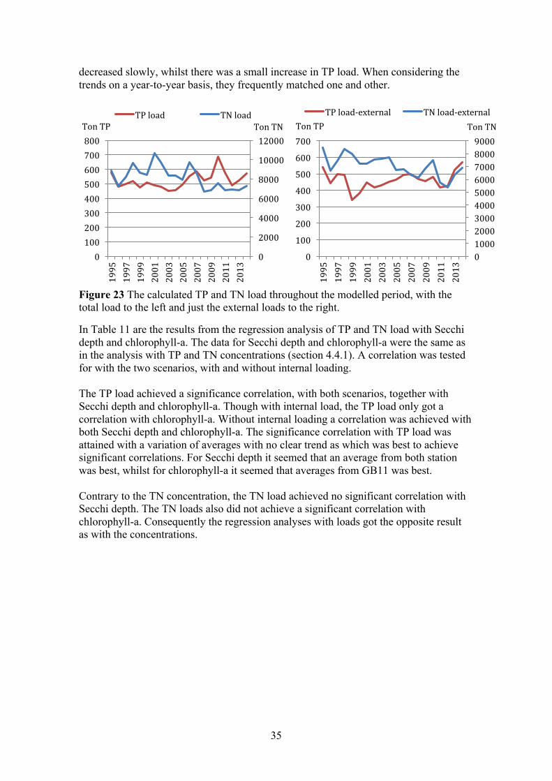
35

decreased slowly, whilst there was a small increase in TP load. When considering the trends on a year-to-year basis, they frequently matched one and other.


In Table 11 are the results from the regression analysis of TP and TN load with Secchi depth and chlorophyll-a. The data for Secchi depth and chlorophyll-a were the same as in the analysis with TP and TN concentrations (section 4.4.1). A correlation was tested for with the two scenarios, with and without internal loading. The TP load achieved a significance correlation, with both scenarios, together with Secchi depth and chlorophyll-a. Though with internal load, the TP load only got a correlation with chlorophyll-a. Without internal loading a correlation was achieved with both Secchi depth and chlorophyll-a. The significance correlation with TP load was attained with a variation of averages with no clear trend as which was best to achieve significant correlations. For Secchi depth it seemed that an average from both station was best, whilst for chlorophyll-a it seemed that averages from GB11 was best. Contrary to the TN concentration, the TN load achieved no significant correlation with Secchi depth. The TN loads also did not achieve a significant correlation with chlorophyll-a. Consequently the regression analyses with loads got the opposite result as with the concentrations.

0

2000

4000

6000

8000

10000

12000

0100200300400500600700800

1995

1997

1999

2001

2003

2005

2007

2009

2011

2013


0100020003000400050006000700080009000

0100200300400500600700

1995

1997

1999

2001

2003

2005

2007

2009

2011

2013


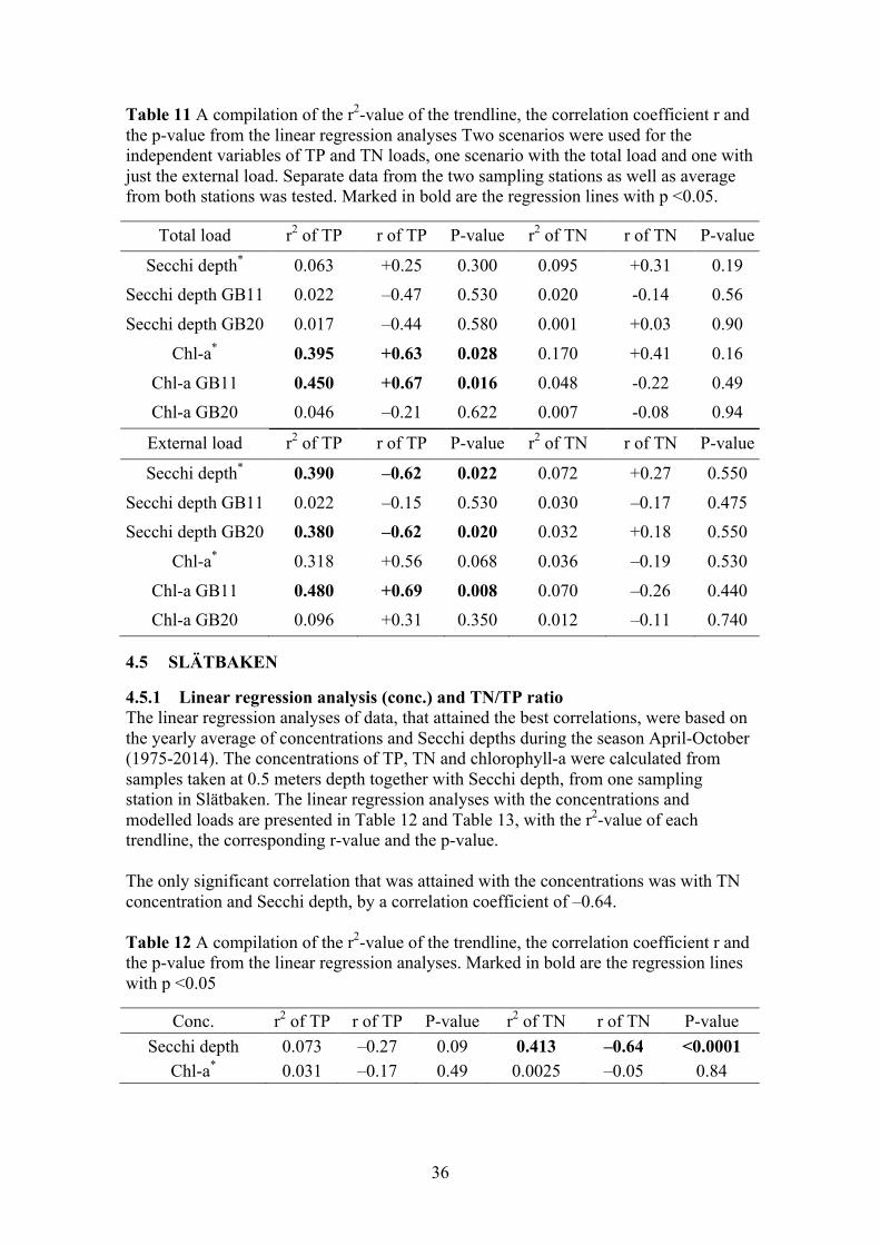
36

Table 11 A compilation of the r2-value of the trendline, the correlation coefficient r and the p-value from the linear regression analyses Two scenarios were used for the independent variables of TP and TN loads, one scenario with the total load and one with just the external load. Separate data from the two sampling stations as well as average from both stations was tested. Marked in bold are the regression lines with p <0.05.


Secchi depth* 0.063 +0.25 0.300 0.095 +0.31 0.19 Secchi depth GB11 0.022 –0.47 0.530 0.020 -0.14 0.56

Secchi depth GB20 0.017 –0.44 0.580 0.001 +0.03 0.90

Chl-a* 0.395 +0.63 0.028 0.170 +0.41 0.16

Chl-a GB11 0.450 +0.67 0.016 0.048 -0.22 0.49 Chl-a GB20 0.046 –0.21 0.622 0.007 -0.08 0.94


Secchi depth* 0.390 –0.62 0.022 0.072 +0.27 0.550

Secchi depth GB11 0.022 –0.15 0.530 0.030 –0.17 0.475 Secchi depth GB20 0.380 –0.62 0.020 0.032 +0.18 0.550

Chl-a* 0.318 +0.56 0.068 0.036 –0.19 0.530

Chl-a GB11 0.480 +0.69 0.008 0.070 –0.26 0.440 Chl-a GB20 0.096 +0.31 0.350 0.012 –0.11 0.740

4.5 SLÄTBAKEN

4.5.1 Linear regression analysis (conc.) and TN/TP ratio The linear regression analyses of data, that attained the best correlations, were based on the yearly average of concentrations and Secchi depths during the season April-October (1975-2014). The concentrations of TP, TN and chlorophyll-a were calculated from samples taken at 0.5 meters depth together with Secchi depth, from one sampling station in Slätbaken. The linear regression analyses with the concentrations and modelled loads are presented in Table 12 and Table 13, with the r2-value of each trendline, the corresponding r-value and the p-value. The only significant correlation that was attained with the concentrations was with TN concentration and Secchi depth, by a correlation coefficient of –0.64. Table 12 A compilation of the r2-value of the trendline, the correlation coefficient r and the p-value from the linear regression analyses. Marked in bold are the regression lines with p <0.05

Conc. r2 of TP r of TP P-value r2 of TN r of TN P-value Secchi depth 0.073 –0.27 0.09 0.413 –0.64 <0.0001

Chl-a* 0.031 –0.17 0.49 0.0025 –0.05 0.84

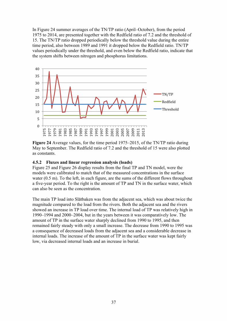
37

In Figure 24 summer averages of the TN/TP ratio (April–October), from the period 1975 to 2014, are presented together with the Redfield ratio of 7.2 and the threshold of 15. The TN/TP ratio dropped periodically below the threshold value during the entire time period, also between 1989 and 1991 it dropped below the Redfield ratio. TN/TP values periodically under the threshold, and even below the Redfield ratio, indicate that the system shifts between nitrogen and phosphorus limitations.


4.5.2 Fluxes and linear regression analysis (loads) Figure 25 and Figure 26 display results from the final TP and TN model, were the models were calibrated to match that of the measured concentrations in the surface water (0.5 m). To the left, in each figure, are the sums of the different flows throughout a five-year period. To the right is the amount of TP and TN in the surface water, which can also be seen as the concentration. The main TP load into Slätbaken was from the adjacent sea, which was about twice the magnitude compared to the load from the rivers. Both the adjacent sea and the rivers showed an increase in TP load over time. The internal load of TP was relatively high in 1990–1994 and 2000–2004, but in the years between it was comparatively low. The amount of TP in the surface water sharply declined from 1990 to 1995, and then remained fairly steady with only a small increase. The decrease from 1990 to 1995 was a consequence of decreased loads from the adjacent sea and a considerable decrease in internal loads. The increase of the amount of TP in the surface water was kept fairly low, via decreased internal loads and an increase in burial.

0510152025303540

1975

1977

1979

1981

1983

1985

1987

1989

1991

1993

1995

1997

1999

2001

2003

2005

2007

2009

2011

2013


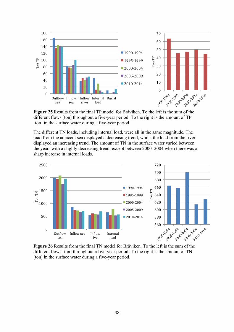
38

Figure 25 Results from the final TP model for Bråviken. To the left is the sum of the different flows [ton] throughout a five-year period. To the right is the amount of TP [ton] in the surface water during a five-year period.

The different TN loads, including internal load, were all in the same magnitude. The load from the adjacent sea displayed a decreasing trend, whilst the load from the river displayed an increasing trend. The amount of TN in the surface water varied between the years with a slighly decreasing trend, except between 2000–2004 when there was a sharp increase in internal loads.

Figure 26 Results from the final TN model for Bråviken. To the left is the sum of the different flows [ton] throughout a five-year period. To the right is the amount of TN [ton] in the surface water during a five-year period.

020406080100120140160180

Out.lowsea

In.lowsea

In.lowriver

Internalload

Burial

TonT

P

1990-19941995-19992000-20042005-20092010-2014

0

10

20

30

40

50

60

70

TonT

P

0

500

1000

1500

2000

2500

Out.lowsea

In.lowsea In.lowriver

Internalload

TonT

N

1990-1994

1995-1999

2000-2004

2005-2009

2010-2014

560580600620640660680700720

TonT

N

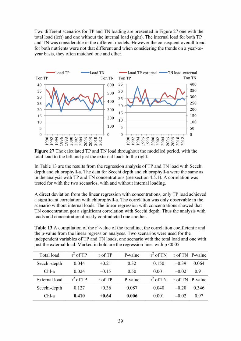
39

Two different scenarios for TP and TN loading are presented in Figure 27 one with the total load (left) and one without the internal load (right). The internal load for both TP and TN was considerable in the different models. However the consequent overall trend for both nutrients were not that different and when considering the trends on a year-to-year basis, they often matched one and other.


In Table 13 are the results from the regression analysis of TP and TN load with Secchi depth and chlorophyll-a. The data for Secchi depth and chlorophyll-a were the same as in the analysis with TP and TN concentrations (see section 4.5.1). A correlation was tested for with the two scenarios, with and without internal loading. A direct deviation from the linear regression with concentrations, only TP load achieved a significant correlation with chlorophyll-a. The correlation was only observable in the scenario without internal loads. The linear regression with concentrations showed that TN concentration got a significant correlation with Secchi depth. Thus the analysis with loads and concentration directly contradicted one another. Table 13 A compilation of the r2-value of the trendline, the correlation coefficient r and the p-value from the linear regression analyses. Two scenarios were used for the independent variables of TP and TN loads, one scenario with the total load and one with just the external load. Marked in bold are the regression lines with p <0.05


Secchi-depth 0.044 +0.21 0.32 0.150 –0.39 0.064 Chl-a 0.024 –0.15 0.50 0.001 –0.02 0.91


Secchi-depth 0.127 +0.36 0.087 0.040 –0.20 0.346 Chl-a 0.410 +0.64 0.006 0.001 –0.02 0.97

0

100

200

300

400

500

600

0510152025303540

1990

1992

1994

1996

1998

2000

2002

2004

2006

2008

2010

2012

TonTNTonTPLoadTP LoadTN

050100150200250300350400

05101520253035

1990

1992

1994

1996

1998

2000

2002

2004

2006

2008

2010

2012

TonTNTonTPLoadTP-external TNload-external

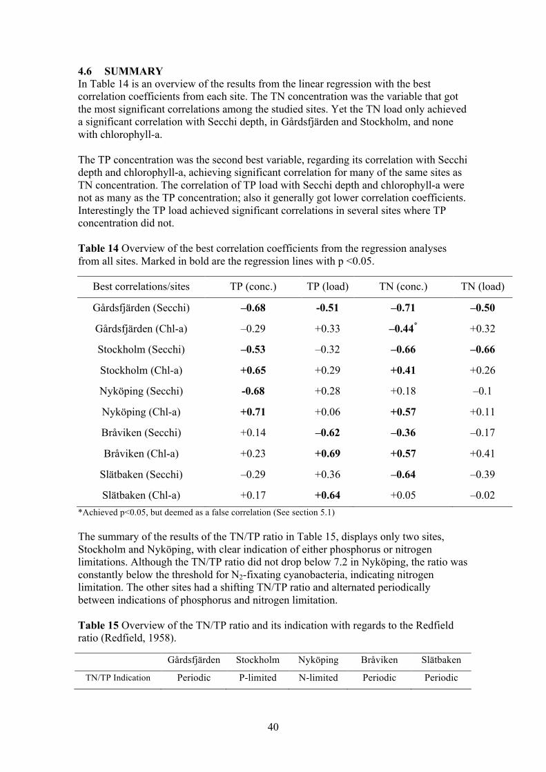
40

4.6 SUMMARY In Table 14 is an overview of the results from the linear regression with the best correlation coefficients from each site. The TN concentration was the variable that got the most significant correlations among the studied sites. Yet the TN load only achieved a significant correlation with Secchi depth, in Gårdsfjärden and Stockholm, and none with chlorophyll-a. The TP concentration was the second best variable, regarding its correlation with Secchi depth and chlorophyll-a, achieving significant correlation for many of the same sites as TN concentration. The correlation of TP load with Secchi depth and chlorophyll-a were not as many as the TP concentration; also it generally got lower correlation coefficients. Interestingly the TP load achieved significant correlations in several sites where TP concentration did not. Table 14 Overview of the best correlation coefficients from the regression analyses from all sites. Marked in bold are the regression lines with p <0.05.

Best correlations/sites TP (conc.) TP (load) TN (conc.) TN (load)

Gårdsfjärden (Secchi) –0.68 -0.51 –0.71 –0.50

Gårdsfjärden (Chl-a) –0.29 +0.33 –0.44* +0.32

Stockholm (Secchi) –0.53 –0.32 –0.66 –0.66

Stockholm (Chl-a) +0.65 +0.29 +0.41 +0.26

Nyköping (Secchi) -0.68 +0.28 +0.18 –0.1

Nyköping (Chl-a) +0.71 +0.06 +0.57 +0.11

Bråviken (Secchi) +0.14 –0.62 –0.36 –0.17

Bråviken (Chl-a) +0.23 +0.69 +0.57 +0.41

Slätbaken (Secchi) –0.29 +0.36 –0.64 –0.39

Slätbaken (Chl-a) +0.17 +0.64 +0.05 –0.02 *Achieved p<0.05, but deemed as a false correlation (See section 5.1) The summary of the results of the TN/TP ratio in Table 15, displays only two sites, Stockholm and Nyköping, with clear indication of either phosphorus or nitrogen limitations. Although the TN/TP ratio did not drop below 7.2 in Nyköping, the ratio was constantly below the threshold for N2-fixating cyanobacteria, indicating nitrogen limitation. The other sites had a shifting TN/TP ratio and alternated periodically between indications of phosphorus and nitrogen limitation. Table 15 Overview of the TN/TP ratio and its indication with regards to the Redfield ratio (Redfield, 1958).

Gårdsfjärden Stockholm Nyköping Bråviken Slätbaken

TN/TP Indication Periodic P-limited N-limited Periodic Periodic

41

5 DISCUSSION The results from the linear regression analyses varied extensively (Table 14), with no single nutrient clearly limiting at any of the sites. The assessment of the limiting nutrient was made difficult by the duality of the results. At all of the sites, either the load or concentration of both nutrients gave a significant correlation with Secchi depth and/or chlorophyll-a. Offering little support to an explanation to which nutrient was generally the limiting one. However for some of the sites there is an explanation for the similar results in regards to nitrogen and phosphorus. As a consequence of nitrogen and phosphorus being essential nutrients in phytoplankton, there is often a matching trend between TP and TN concentration (Walve and Rolff, 2016). This matching trend between TP and TN concentration was observed in all of the sites and true for most years (Appendix F). The result of this was particularly apparent in Gårdsfjärden and Stockholm. In every analysis were TP concentration gave a significant correlation, the TN concentration correspondingly gave a significant correlation (Table 14). This does not answer the question of which nutrient was limiting, but it explains the dual correlations for some sites. Moreover the dual correlations in some sites likely signify the natural role for one nutrient as an essential nutrient and not the limiting nutrient. The tendency for matching trends for TP and TN concentration was why a correlation with loads was also tested. The magnitude of the loads together with internal processes regulates the concentration of nutrients in the water. However it was assumed that there would not necessarily be a matching correlation between the TP and TN loads. The expectation was therefore that the loads would better indicate what nutrient was limiting, as it was anticipated they followed separate trends, but that there would still be a clear relationship with Secchi depth and chlorophyll-a. In similar studies, such as in Stockholm in the early 1970s (Brattberg, 1986), Himmerfjärden (Elmgren and Larsson, 1997), Neuse River Estuary (Paerl et al., 2004) and the Lakes Experiments (Schindler et al., 2008) the crucial factor was that the load from only one nutrient was changed at a time. This enabled the scientists to examine the response from the systems, without having to account for a dual reduction of nutrients. Unfortunately, in most of the studied sites the loading trends, with and without internal loading, displayed the same matching trend as with the concentrations (Figure 11, Figure 15, Figure 19, Figure 23, and Figure 27). Although for Gårdsfjärden and Stockholm there were instances with changes in loading for only one nutrient. In Gårdsfjärden the phosphorus load decreased between 2010 and 2012 (Figure 11), which was investigated without result regarding a response in chlorophyll-a (Appendix D). The result of the decreased phosphorus load was also observed in the phosphorus concentration (Appendix D). For Stockholm there was a sharp decrease in nitrogen load from 1990 until 1997 (Figure 15), but no clear response in chlorophyll-a was identified (Appendix D). Surprisingly the decrease in TN load was not observed in the TN concentration. This could indicate that the TN concentration was kept relatively constant via an influx of nitrogen from N2-fixating cyanobacteria. An additional problem was that for three of the five sites, samples were only taken from the upper 0.5 meters of surface water. As it was supposed to be the upper 0–10 meter used in the calibration and subsequent calculation of internal loading, this was made uncertain. As a consequence, and depending on the hydrological condition, the internal load might not have been representative in those sites.

42

This was also shown in Appendix B, were the difference in average concentration from 0.5 meter and 0–10 meters was examined for Gårdsfjärden. The biggest difference in using the different depth was a higher average concentration for 0.5 meter. Consequently the sites that only had continuous measurements in the upper 0.5 meters could have an overestimated internal loading. Another general problem with the modelled loads was that the model was run on a yearly basis. In areas were the TN and TP load vary significantly during the year, the yearly average might not match that of the load during the summer months, for which the averages of Secchi depth and chlorophyll-a was calculated. This problem is discussed further in the site-specific analysis. One factor that should also be taken into consideration, when evaluating the approach, was that the sampling programs were not purposely designed for it. For all the sites the sampling data were heterogeneously distributed, changing in frequency and extent over the years. To obtain averages that are representative, the samplings programs should preferably be constant over the years. The effect of the dispersed data was hard to evaluate, as most sites achieved some correlation between concentrations. Though it is likely this was the cause for some of the sites not displaying a greater relationship between TP or TN and Secchi depth and chlorophyll-a. The overall inconclusive results could have been a consequence of unfavourable conditions for example, by the matching trends in both concentrations and loads or the heterogeneously distributed data. It is however possible that the problem was with the general approach used to define nutrient-limited systems and the choice of method. The hypothesis was that either one or the other nutrient would be the long-term limiting nutrient, disregarding any short-scale changes. Consequently, the choice in method did not account for the possibility of co-limited systems. Most co-limited coastal areas are limited by both nitrogen and phosphorus, but during different seasons of the year (Conley, 1999). An example of this is the inner Oslofjord, were nitrogen limits the spring phytoplankton blooms and phosphorus limits the summer and autumn blooms (Paasche and Erga, 1988). Another example is that in many Danish estuaries the phytoplankton is limited by phosphorus in the spring, and then change to nitrogen limitation in the summer (Conley et al., 2000; Carstensen et al., 2006). Also in Himmerfjärden, which is described as nitrogen limited, there was a change from nitrogen to phosphorus limitation during two years (Elmgren and Larsson, 1997; Elmgren and Larsson, 2001; Howarth and Marino, 2006). A connection to the TN/TP ratio for several of the sites seems apparent, as it often indicated a periodical shift between phosphorus and nitrogen limitation. For this study, if a change in the limiting nutrient happened during the studied annual period, it would not be detectable with the linear regression approach. The probable result would be a low or no correlation between the nutrients and eutrophication-indicators. The choice in the yearly period was an iterative process, meaning the period with the best correlation was chosen. Subsequently, any changes in the limited nutrient might, through design, have been missed. Especially since there is often a weaker relationship between the spring blooms and the limiting nutrient (Conley, 1999). Subsequently if any of the sites were co-limited the results will only reveal the limiting nutrient during the summer season. Though for the sites that the TN/TP ratio indicated a change between years, the linear approach was still uncertain.

43

With the problem of matching trends, in both concentrations and loads, an overall conclusion was hard to express. Also, there were site-specific factors that should be considered when assessing the results. Therefore an individual analysis of each area is discussed below.

5.1 Gårdsfjärden In Gårdsfjärden the regression analysis revealed that both TN and TP gave equivalent correlation coefficients regarding Secchi depth (Table 14). None of the nutrients showed a realistic statistically significant correlation with chlorophyll-a. A problem with the site that emerged late in the study, was that the paper mill had released large quantities of toxins and organic matter. The negative correlation in Table 14 with TN concentration and chlorophyll-a could be a consequence of this. Both the concentrations and loads also showed an overall matching trend. This made it difficult to discern if one correlation indicated the limiting nutrient and if one was just a natural the correlation. The results from the TN/TP ratio were also inconclusive, with the ratio fluctuating around the threshold-value with no clear trend. No conclusion as to the limiting nutrient could be made.

5.2 Stockholm’s inner archipelago Similarly to Gårdsfjärden, in Stockholm’s inner archipelago both TP and TN concentration got a statistically significant correlation with Secchi depth. The concentrations also achieved significant correlation with chlorophyll-a. Yet with the loads, none but the TN load together with Secchi depth got a significant correlation. As the concentration should be dependent on the internal and external load, this result was unexpected. Especially since the TN concentration got a significant correlation with chlorophyll-a whilst the load did not. The reason for the TP load not achieving the same significant correlation as TP concentration could be because of a lot of phosphorus was buried in the sediments (Figure 13). But the most probable reason would be the difference in yearly loads and the load during the summer months. If the difference in loads were significant, it would explain why they did not achieve the same level of correlation as the concentrations. Contrary to Gårdsfjärden, the TN/TP ratio in Stockholm was constantly well above the threshold and Redfield ratio, indicating a long-term phosphorous limited system (Redfield, 1958; Håkanson and Bryhn, 2008). This implies that the correlation between TN, Secchi depth and chlorophyll-a, could signify the natural correlation of nitrogen as an essential nutrient, but not the limiting nutrient. This theory has further backing when considering that a decrease in nitrogen load did not affect the TN or chlorophyll-a concentration (Appendix D and Figure 15). This would mean that Stockholm’s inner archipelago has remained phosphorous limited since the 1970s, when studied by Brattberg (1986). Though this could not be confirmed by the linear regression analysis.

44

5.3 The Bays of Nyköping The Bays of Nyköping showed indications of being phosphorous limited, with TP concentration achieving the best correlation coefficient for both Secchi depth and chlorophyll-a (Table 14). The significant correlation between TN concentration and chlorophyll-a was comparatively much lower and could be explained as a natural correlation. Similarly to Stockholm, the TP and TN loads did not correlate well with either Secchi depth or chlorophyll-a. The risk that this was due to the usage of yearly loads seems likely. Particularly since the budget calculation showed that it was the rivers that dominated the load of both TP and TN (Figure 17 and Figure 18). As the rivers discharge significantly varies over the course of a year, the loads would as well. The impact of the rivers inflow was also reflected in the salinity level in Table 1, were the Bays of Nyköping had the lowest salinity of all studied sites. The TN/TP ratio in the Bays of Nyköping stayed between the threshold and Redfield ratio (Redfield, 1958), which suggest a nitrogen limited system with condition favourable for N2-fixating cyanobacteria (Håkanson and Bryhn, 2008). This might seem contradictory to the results from the linear regression, but it could be explained with the theory regarding P-limitations from (Schindler et al., 2008). If the N2-fixating cyanobacteria were able to maintain the phytoplankton’s relative biomass to the concentration of phosphorus, even in periods of low concentrations of nitrogen, the system would be phosphorous limited and still have a TN/TP ratio under 15. One factor that might contradict this theory was the low residence time in the bays. N2-fixating cyanobacteria thrive in warm, calm and vertically stratified water, where they can migrate between the nutrient rich bottom and the surface waters (Paerl et al., 2001). Having a short residence time, as in case of the Bays of Nyköping, disrupts the growth rates and structural integrity of N2-fixating cyanobacteria, making it difficult for them to grow (Paerl et al., 2001; Paerl, 2009). Though it is possible that during periods of the summer the condition were favourable for N2-fixating cyanobacteria. It seems unlikely it was a long-lasting state in the bays. Nevertheless the results from the linear regression arguably points towards a phosphorous limited system.

5.4 Bråviken In Bråviken the analysis with concentrations and the load directly contradicted each other. The loads indicated P-limitation, whilst the analysis with the concentrations implied N-limitation. The TN/TP ratio fluctuated over the years, indicating shifts between N- and P-limitations but no conclusive result. Therefore it became an evaluation of the correlation coefficients. The methods for attaining representable concentration in Bråviken differed from the other sites, with the concerns that the river’s possible effect on sampling station GB11 (Asklund and Fridlund, 2004). Though no evidence could be found of GB11 being visibly affected by the river (Appendix F), each station data was still tested separately, as well as an average calculated from both station. For Secchi depth, a correlation was only found when considering an average from both stations. The TP load achieved a twice as high a correlation coefficient as with TN concentration. Making it unquestionably the better variable to describe Secchi depth. For the chlorophyll-a, the result was more complicated to evaluate.

45

The TP load got a slightly higher correlation coefficient than TN concentration. However, for TN concentration a significant correlation was only achieved with values from station GB20, whereas for TP load it was attained with averages from both stations and with data from GB11, but not for GB20. No clear explanation for the discrepancy between using averages from both stations and individual stations could be established. With TP load getting higher correlation coefficients with both Secchi depth and chlorophyll-a the results imply phosphorus limited system. Though co-limitation could not fully be dismissed.

5.5 Slätbaken In Slätbaken the analysis with concentrations and the load also contradicted each other. Both TN concentration and TP load got exactly equal correlation coefficient but with Secchi depth and chlorophyll-a respectively. As both variables are symptoms and measurements of eutrophication it was impossible to draw any conclusion as to the limiting nutrient. The TN/TP ratio also did not reveal any conclusive support either, only an indication of changes between nitrogen and phosphorus limitations over the years, with the ratio even dropping below the Redfield ratio. Possibly indicating a co-limitation with both nutrients.

6 CONCLUSIONS The method of using linear regression analysis to compare empirical data of nutrient availability (averages of TP and TN) with estimates of eutrophication (Secchi depth and chlorophyll-a) to determine the limiting nutrient was not in itself conclusive. This was mostly due to TP and TN concentration having naturally matching trends; consequently both nutrients often achieved equivalent correlations coefficients in the analyses. Applying mass-balance calculation, with empirical data, to determine the internal and external load of TP and TN and subsequently test these for correlations with Secchi depth and chlorophyll-a was mostly unsuccessful. This was partly due to the matching trends in TP and TN loads, which led to the same problems as with the concentrations. A plausible reason for not achieving more significant correlation was because the loads were calculated on a yearly basis, whilst the Secchi depth and chlorophyll-a were summer averages. The mass-balance calculations should be scaled down to a shorter modelled period to encompass the same summer period, which could lead to better correlations. Combining the results from the two linear regression analyses with the TN/TP ratio to determine the limiting nutrient did result in some conclusions. For three of the sites, Stockholm’s inner archipelago, the Bays of Nyköping and Bråviken the combined results signified these as being limited by phosphorus. But it should be noted that it was mostly a lack of conclusive results from two of the three methods in each site that led to these conclusions, and not collaborating results from two or more methods. As for the other sites no conclusion regarding the limiting nutrient could be drawn. Ultimately, it was hard to achieve more conclusive results from utilizing empirical data, since the sampling data was heterogeneously dispersed. Also having matching trends in both concentrations as well as loads made any observation of the limiting nutrient problematic to distinguish.

46

Using more complex statistical methods might achieve more definite results, however the linear regression approach is considered simple but robust. Even with problematic data the linear regression approach is a proven method. Furthermore other more complex statistical methods require additional variables, a higher sampling frequency and generally more extensive data, which were not available for most sites. Conducting further large-scale experiments in coastal areas, where one nutrient is changed and the other is kept comparatively constant, would provide better data to evaluate nutrient limitation. The problem with such an experiment is how to control inflow of nutrients from the adjacent sea. As this parameter cannot really be controlled, it would be difficult conduct an experiment with the level of certainty as that obtained in the Lake-Experiments.

47

7 REFERENCES Asklund, R. and Fridlund, M., (2004). Dynamisk fosformodellering för Bråviken. Uppsala University. Department of Ecology and Genetics. Brattberg, G., (1986). Decreased Phosphorus Loading Changes Phytoplankton Composition and Biomass in the Stockholm Archipelago. Vatten 1986 (2), pp.141–153. Brown, T. and Simpson, J., (2001). Managing Phosphorus Inputs to Urban Lakes: I. Determining the Trophic State of Your Lake. Watershed Protection Techniques 3(4), pp. 771-781. Carstensen, J., Conley, D.J., Andersen, J.H. and Ærtebjerg, G., (2006). Coastal Eutrophication and Trend Reversal: A Danish Case Study. Limnology and Oceanography 51(1), pp.398–408.

Conley, D.J., (1999). Biogeochemical nutrient cycles and nutrient management strategies. Hydrobiologia 410, pp.87–96. Conley, D.J., Kaas, H., Møhlenberg, F., Rasmussen, B. and Windolf, J., (2000). Characteristics of Danish estuaries. Estuaries, 23(6), pp.820–837. Conley, D.J., Paerl, H.W., Howarth, R.W., Boesch, D.F., Seitzinger, S.P., Havens, K.E., Lancelot, C. and Likens, G.E., (2009). Controlling eutrophication: nitrogen and phosphorus. Science 323, pp.1014–1015. Elmgren, R. and Larsson, U., (2001). Nitrogen and the Baltic Sea: Managing Nitrogen in Relation to Phosphorus. The Scientific World 1(S2), pp.371–377. Elmgren, R. and Larsson, U., (1997). Himmerfjärden-Changes in a nutrient enriched coastal ecosystem. Stockholm: Swedish Environmental Protection Agency. Report 5587 (Summary in English pp. 13-18) Granéli, E., Wallström, K., Larsson, U., Granéli W. and Elmgren, R., (1990). Nutrient Limitation of Primary Production in the Baltic Sea Area. Ambio Marine Eutrophication 19(3), pp.142–151. Håkanson, L. and Bryhn, A.C., (2008). Eutrophication in the Baltic Sea: present situation, nutrient transport processes, remedial strategies. Berlin: Springer. ISBN: 978-3-540-70908-4 Håkanson, L., Bryhn, A.C. and Hytteborn, J.K., (2007). On the issue of limiting nutrient and predictions of cyanobacteria in aquatic systems. Science of The Total Environment 379, pp.89–108. doi:10.1016/j.scitotenv.2007.03.009

HELCOM, (2009). Eutrophication in the Baltic Sea – An integrated thematic assessment of the effects of nutrient enrichment and eutrophication in the Baltic Sea region. Balt. Sea Environ. Proc. No. 115B.

48

Howarth, R.W. and Marino, R., (2006). Nitrogen as the limiting nutrient for eutrophication in coastal marine ecosystems: Evolving views over three decades. Limnology and Oceanography 51(1), pp.364–376. doi:10.4319/lo.2006.51.1_part_2.0364 Karlsson, O.M., Malmaeus, J.M., Viktor, T., Andersson, M.G. and Rydin, E., (2014). A revised semi-empirical mass balance model for phosphorus in Baltic coastal areas. Fundamental and Applied Limnology 185(3), pp.209–221. doi:10.1127/fal/2014/0613 Körner S and Wahlgren L., (2005). Statistiska metoder - andra upplagan. Lund: Studentlitteratur, pp 70-78 & 130-131. ISBN: 91-44-04420-8. (In Swedish) Lindgren, G., (2004). God ekologisk status enligt ramdirektivet för vatten- En rapport från miljöövervakningen i Gävleborgs län. Gävleborgs County’s Administrative Board. Report 2004:3. [Online] Available at: <http://www.lansstyrelsen.se/gavleborg/SiteCollectionDocuments/Sv/publikationer/2004/2004_3.pdf> [Accessed 29 May 2017] (In Swedish) Lücke, J., (2016). Undersökningar i Stockholms skärgård 2015. Vattenkemi och plankton. Stockholm Vatten AB. [Online] Available at: <http://www.stockholmvattenochavfall.se/globalassets/pdf1/rapporter/vattenvard/skargarden/skargardsrapporten-2015.pdf> [Accessed 29 May 2017] (In Swedish) Olsson, H., (2002). Kustzonsmodell för norra delarna av Östergötlands skärgård. Resultat för perioden 1985–2000. Swedish Meteorological and Hydrological Institute, [Online] Available at: <http://www.lansstyrelsen.se/ostergotland/SiteCollectionDocuments/sv/miljo-och-klimat/tillstandet-i-miljon/miljoovervvakning/kust-och-hav/Kustzonsmodell_Norr_85t01.pdf>[Accessed 29 May 2017] (In Swedish) Paasche, E. and Erga, S.R., (1988). Phosphorus and nitrogen limitation of phytoplankton in the inner Oslofjord (Norway). Sarsia 73, pp.229–243. doi:10.1080/00364827.1988.10413409 Paerl, H.W., (2009). Controlling Eutrophication along the Freshwater—Marine Continuum: Dual Nutrient (N and P) Reductions are Essential. Estuaries Coasts 32, pp.593–601. Paerl, H.W., Fulton, R.S., Moisander, P.H. and Dyble, J., (2001). Harmful freshwater algal blooms, with an emphasis on cyanobacteria. The Scientific World Journal 1, pp.76–113. doi:10.1100/tsw.2001.16 Paerl, H.W., Valdes, L.M., Joyner, A.R., Piehler, M.F. and Lebo, M.E., (2004). Solving Problems Resulting from Solutions: Evolution of a Dual Nutrient Management Strategy for the Eutrophying Neuse River Estuary, North Carolina. Environmental Science & Technology 38, pp.3068–3073. doi:10.1021/es0352350 Ptacnik, R., Andersen, T. and Tamminen, T., (2010). Performance of the Redfield Ratio and a Family of Nutrient Limitation Indicators as Thresholds for Phytoplankton N vs. P Limitation. Ecosystems 13, pp.1201–1214. doi:10.1007/s10021-010-9380-z

49

Redfield, A.C., (1958). The biological control of chemical factors in the environment. American Scientist 46(3), pp.230A, 205–221. Schindler, D.W., Hecky, R.E., Findlay, D.L., Stainton, M.P., Parker, B.R., Paterson, M.J., Beaty, K.G., Lyng, M. and Kasian, S.E.M., (2008). Eutrophication of lakes cannot be controlled by reducing nitrogen input: Results of a 37-year whole-ecosystem experiment. Proceedings of the National Academy of Sciences 105(32), pp.11254–11258. doi:10.1073/pnas.0805108105 Schindler, D.W., Vallentyne, J.R., (2008). The Algal Bowl-Overfertilization of the World’s Freshwaters and Estuaries. Edmonton, Alberta, Canada: The University of Alberta Press. ISBN: 978-o-88864-484-8 SLU, (2017). Databank för vattenkemi-flodmynningar-transportberäkningar. Swedish University of Agricultural Sciences (SLU) [Online] Available at: http://webstar.vatten.slu.se/db.html [Accessed 30 May 2017] SMHI, (2003). Djupdata för havsområden 2003. Swedish Meteorological and Hydrological Institute (SMHI). Oceanografi 73, Table 1. (In Swedish) SMHI, (2017a). HYPE. Swedish Meteorological and Hydrological Institute (SMHI) [Online] Available at: <http://www.smhi.se/en/research/research-departments/hydrology/hype-1.7994>[Accessed 30 May 2017] SMHI, (2017b). Vattenwebb-Ladda ner modelldata per område. Swedish Meteorological and Hydrological Institute (SMHI) [Online] Available at: <http://vattenweb.smhi.se/modelarea/>[Accessed 30 May 2017] SMHI, (2017c). Vattenwebb-ladda ner mätning. Swedish Meteorological and Hydrological Institute (SMHI) [Online] Available at: <http://vattenweb.smhi.se/station/> [Accessed 30 May 2017] Svärd, C., (2015). Motala ströms vattenvårdsförbund-2015. Alcontrol AB. [Online] Available at: <http://motalastrom.se/download/resultat/2015/MSV-2015-inkl-bilagor-2015-05-15.pdf>[Accessed 29 May 2017] (In Swedish) Swedish EPA, (2006). Övergödningen av Sveriges kuster och hav. Stockholm: Swedish Enviromental Protection Agency. Report 5587. (Summary in English p.8-10) Walve, J., Rolff, C., (2012). Svealands kustvattenvårdsförbund-Årsrapport 2012, Svealands kustvattenvårdsförbund. [Online] Available at: <http://www.havet.nu/dokument/Svealandskusten2012.pdf>[Accessed 29 May 2017] (In Swedish) Walve, J., Rolff, C., (2016). Svealands kustvattenvårdsförbund- Årsrapport 2016. [Online] Available at: < http://havet.nu/dokument/Svealandskusten2016.pdf> [Accessed 29 May 2017] (In Swedish)

50

Personal communication Blomqvist S. [email protected], (2017). Utsläppsdata för Brandholmen reningsverk [email] Message to Persson M. [[email protected]] Data sent 14 March 2017 Karlsson M. [email protected], (2017). Modellering [email] Message to Persson M. [[email protected]] Data sent 23 March 2017 Kuhla P. [email protected], (2017). Utsläppdata Bravikens pappersbruk [email] Message to Persson M. [[email protected]] Data sent 22 March 2017 Lundgren V. [email protected], (2017). Mätdata för bl.a. kväve och fosfor i Gårdsfjärden [email] Message to Persson M. [[email protected]] Data sent 13 February 2017 Melander E. [email protected], (2017). Historisk data för provpunkter [email] Message to Persson M. [[email protected]] Data sent 24 January and 27 February 2017 Nydahl A. [email protected], (2017). Hämta data [email] Message to Persson M. [[email protected]] Data sent 20 February 2017 Rydh C. [email protected], (2017). Utsläppdata för Slottshagenreningsverk [email] Message to Persson M. [[email protected]] Data sent 6 March 2017 Stockholm Vatten. [email protected], (2017). Rådata för bl.a. kväve och fosfor i Stockholms inre skärgård [email] Message to Persson M. [[email protected]] Data sent 13 January and 25 February 2017

51

APPENDIX A: THEORY OF LINEAR REGRESSION ANALYSIS The program used for linear regression was Excel 2010, with the tools “Statistic toolbox”, “Regression” and “Scatter plot”. The next section gives a short summary of how linear regression works and which statistical variables were gathered and how to interpret them. All theory was taken from Körner and Wahlgren (2005). Linear regression is based on the linear least squares method, were each observation of the independent variable, e.g. TP or TN, is plotted against the corresponding observation of the dependent variable, e.g. Secchi depth or chlorophyll-a. A regression line is then fitted between the points according to Equation 1. In Equation 1 the “a” is a constant, “b” is a coefficient, x is the independent variable and y is the dependent variable.

! = ! + ! ∙ ! (1) The least squares method means that the constant “a” and “b” in Equation 1 is determined so the square sum of Equation 2 is as small as possible. This means that the difference between the actual value and the value on the regression line, also called residuals, becomes as small as possible. Equation 2’s variables have the same definition as in Equation 1.

! − (! + ! ∙ !) ! (2) To determine how strong a linear relationship is the correlation coefficient r is often used. The formula used for calculating the r-value is presented in Equation 3, were x is the independent variable, y is the dependent variable and n is the number of sample pairs.

! = !"! ! !!

!!! ! !! !!! ! !

!

(3)

The calculation returns an r-value that is between -1 and +1, and is interpreted as follows. An r-value equal to -1 means the correlation is negative and all of the observations are on the regression line. An r-value equal to +1 means that the correlation is positive and again all of the observations are on the regression line. If the r-value is close to -1 or +1 this means that there is a strong linear relationship between the independent and dependent variable. The square of r, also called the coefficient of determination (r2), states how much of the total variation of the dependent variable is explained by the linear relationship with the independent variable. So a value of r2, equal to 0.89, means that 89% of the variation for the dependent variable is determined by the independent variable.

52

When using the correlation coefficient to interpret the linear relationship between different variables, it is important to know that the coefficient is easily influenced by extreme values. Plotting the data beforehand and removing any extremes prior to using the linear regression tool avoided this. Also obtained from regression analyses in Excel was the p-value (probvalue) for each regression. The p-value indicates the probability that the null hypothesis is true. The smaller the p-value is the less likely it is that the null hypothesis is true. Generally a p-value of less than five percent means that the trend can be assumed statistically significant.

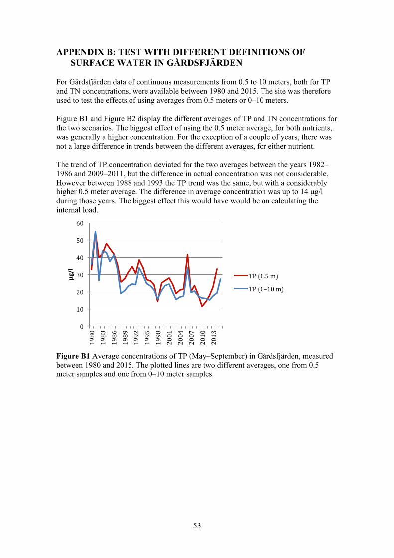
53

APPENDIX B: TEST WITH DIFFERENT DEFINITIONS OF SURFACE WATER IN GÅRDSFJÄRDEN

For Gårdsfjärden data of continuous measurements from 0.5 to 10 meters, both for TP and TN concentrations, were available between 1980 and 2015. The site was therefore used to test the effects of using averages from 0.5 meters or 0–10 meters. Figure B1 and Figure B2 display the different averages of TP and TN concentrations for the two scenarios. The biggest effect of using the 0.5 meter average, for both nutrients, was generally a higher concentration. For the exception of a couple of years, there was not a large difference in trends between the different averages, for either nutrient. The trend of TP concentration deviated for the two averages between the years 1982–1986 and 2009–2011, but the difference in actual concentration was not considerable. However between 1988 and 1993 the TP trend was the same, but with a considerably higher 0.5 meter average. The difference in average concentration was up to 14 µg/l during those years. The biggest effect this would have would be on calculating the internal load.

Figure B1 Average concentrations of TP (May–September) in Gårdsfjärden, measured between 1980 and 2015. The plotted lines are two different averages, one from 0.5 meter samples and one from 0–10 meter samples.

0

10

20

30

40

50

60

1980

1983

1986

1989

1992

1995

1998

2001

2004

2007

2010

2013

μg/l

TP(0.5m)TP(0–10m)

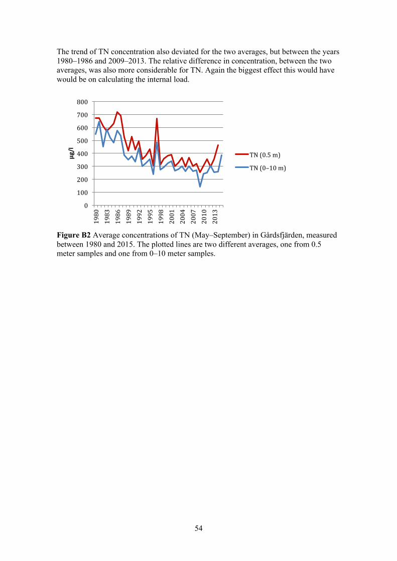
54

The trend of TN concentration also deviated for the two averages, but between the years 1980–1986 and 2009–2013. The relative difference in concentration, between the two averages, was also more considerable for TN. Again the biggest effect this would have would be on calculating the internal load.

Figure B2 Average concentrations of TN (May–September) in Gårdsfjärden, measured between 1980 and 2015. The plotted lines are two different averages, one from 0.5 meter samples and one from 0–10 meter samples.

0100200300400500600700800

1980

1983

1986

1989

1992

1995

1998

2001

2004

2007

2010

2013

μg/l

TN(0.5m)TN(0–10m)

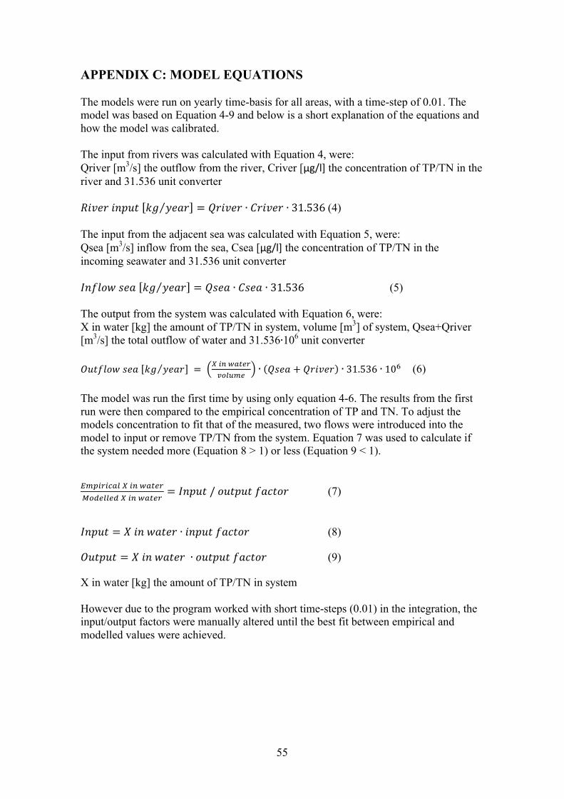
55

APPENDIX C: MODEL EQUATIONS The models were run on yearly time-basis for all areas, with a time-step of 0.01. The model was based on Equation 4-9 and below is a short explanation of the equations and how the model was calibrated. The input from rivers was calculated with Equation 4, were: Qriver [m3/s] the outflow from the river, Criver [μg/l] the concentration of TP/TN in the river and 31.536 unit converter !"#$% !"#$% !" !"#$ = !"#$%" ∙ !"#$%" ∙ 31.536 (4) The input from the adjacent sea was calculated with Equation 5, were: Qsea [m3/s] inflow from the sea, Csea [μg/l] the concentration of TP/TN in the incoming seawater and 31.536 unit converter !"#$%& !"# !" !"#$ = !"#$ ∙ !"#$ ∙ 31.536 (5) The output from the system was calculated with Equation 6, were: X in water [kg] the amount of TP/TN in system, volume [m3] of system, Qsea+Qriver [m3/s] the total outflow of water and 31.536∙106 unit converter !"#$%&' !"# !" !"#$ = ! !" !"#$%

!"#$%& ∙ !"#$ + !"#$%" ∙ 31.536 ∙ 10! (6) The model was run the first time by using only equation 4-6. The results from the first run were then compared to the empirical concentration of TP and TN. To adjust the models concentration to fit that of the measured, two flows were introduced into the model to input or remove TP/TN from the system. Equation 7 was used to calculate if the system needed more (Equation 8 > 1) or less (Equation 9 < 1). !"#$%$&'( ! !" !"#$%!"#$%%$# ! !" !"#$% = !"#$% / !"#$"# !"#$%& (7) !"#$% = ! !" !"#$% ∙ !"#$% !"#$%& (8) !"#$"# = ! !" !"#$% ∙ !"#$"# !"#$%& (9) X in water [kg] the amount of TP/TN in system However due to the program worked with short time-steps (0.01) in the integration, the input/output factors were manually altered until the best fit between empirical and modelled values were achieved.

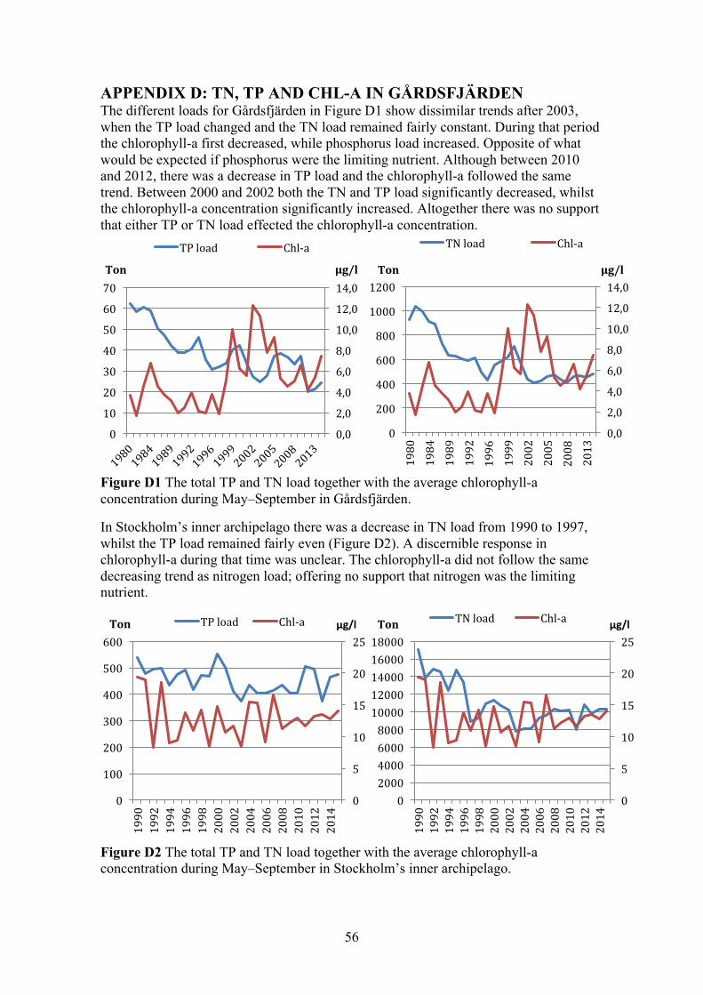
56

APPENDIX D: TN, TP AND CHL-A IN GÅRDSFJÄRDEN The different loads for Gårdsfjärden in Figure D1 show dissimilar trends after 2003, when the TP load changed and the TN load remained fairly constant. During that period the chlorophyll-a first decreased, while phosphorus load increased. Opposite of what would be expected if phosphorus were the limiting nutrient. Although between 2010 and 2012, there was a decrease in TP load and the chlorophyll-a followed the same trend. Between 2000 and 2002 both the TN and TP load significantly decreased, whilst the chlorophyll-a concentration significantly increased. Altogether there was no support that either TP or TN load effected the chlorophyll-a concentration.

Figure D1 The total TP and TN load together with the average chlorophyll-a concentration during May–September in Gårdsfjärden.

In Stockholm’s inner archipelago there was a decrease in TN load from 1990 to 1997, whilst the TP load remained fairly even (Figure D2). A discernible response in chlorophyll-a during that time was unclear. The chlorophyll-a did not follow the same decreasing trend as nitrogen load; offering no support that nitrogen was the limiting nutrient.

Figure D2 The total TP and TN load together with the average chlorophyll-a concentration during May–September in Stockholm’s inner archipelago.

0,02,04,06,08,010,012,014,0

0

200

400

600

800

1000

1200

1980

1984

1989

1992

1996

1999

2002

2005

2008

2013

μg/lTon

TNload Chl-a

0,02,04,06,08,010,012,014,0

010203040506070

μg/lTon

TPload Chl-a

0

5

10

15

20

25

020004000600080001000012000140001600018000

1990

1992

1994

1996

1998

2000

2002

2004

2006

2008

2010

2012

2014

μg/lTon TNload Chl-a

0

5

10

15

20

25

0

100

200

300

400

500

600

1990

1992

1994

1996

1998

2000

2002

2004

2006

2008

2010

2012

2014

μg/lTon TPload Chl-a

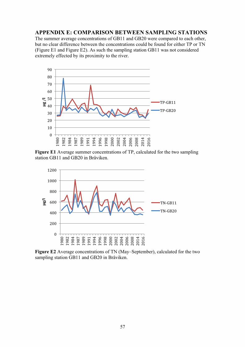
57

APPENDIX E: COMPARISON BETWEEN SAMPLING STATIONS The summer average concentrations of GB11 and GB20 were compared to each other, but no clear difference between the concentrations could be found for either TP or TN (Figure E1 and Figure E2). As such the sampling station GB11 was not considered extremely effected by its proximity to the river.

Figure E1 Average summer concentrations of TP, calculated for the two sampling station GB11 and GB20 in Bråviken.

Figure E2 Average concentrations of TN (May–September), calculated for the two sampling station GB11 and GB20 in Bråviken.

0102030405060708090

1980

1982

1984

1987

1989

1991

1994

1996

1998

2000

2002

2004

2006

2008

2014

2016

μg/l

TP-GB11TP-GB20

0

200

400

600

800

1000

1200

1980

1982

1984

1987

1989

1991

1994

1996

1998

2000

2002

2004

2006

2008

2014

2016

μg/l

TN-GB11TN-GB20

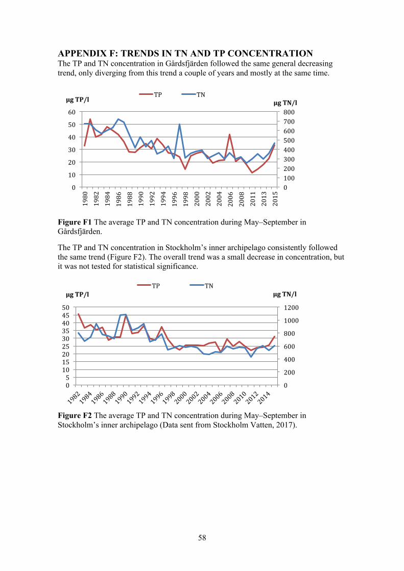
58

APPENDIX F: TRENDS IN TN AND TP CONCENTRATION The TP and TN concentration in Gårdsfjärden followed the same general decreasing trend, only diverging from this trend a couple of years and mostly at the same time.

Figure F1 The average TP and TN concentration during May–September in Gårdsfjärden.

The TP and TN concentration in Stockholm’s inner archipelago consistently followed the same trend (Figure F2). The overall trend was a small decrease in concentration, but it was not tested for statistical significance.

Figure F2 The average TP and TN concentration during May–September in Stockholm’s inner archipelago (Data sent from Stockholm Vatten, 2017).

0100200300400500600700800

0102030405060

1980

1982

1984

1986

1988

1990

1992

1994

1996

1998

2000

2002

2004

2006

2008

2011

2013

2015

μgTN/lμgTP/lTP TN

020040060080010001200

05101520253035404550

μgTN/lμgTP/lTP TN

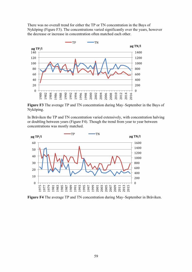
59

There was no overall trend for either the TP or TN concentration in the Bays of Nyköping (Figure F3). The concentrations varied significantly over the years, however the decrease or increase in concentration often matched each other.

Figure F3 The average TP and TN concentration during May–September in the Bays of Nyköping.

In Bråviken the TP and TN concentration varied extensively, with concentration halving or doubling between years (Figure F4). Though the trend from year to year between concentrations was mostly matched.

Figure F4 The average TP and TN concentration during May–September in Bråviken.

0200400600800100012001400

020406080100120140

1980

1982

1984

1986

1988

1990

1992

1994

1996

1998

2000

2002

2004

2006

2008

2010

2012

2014

2016

μgTN/lμgTP/l

TP TN

02004006008001000120014001600

0

10

20

30

40

50

60

1975

1977

1979

1981

1983

1985

1987

1989

1991

1993

1995

1997

1999

2001

2003

2005

2007

2009

2011

2013

2015

μgTN/lμgTP/lTP TN

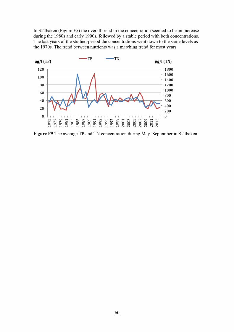
60

In Slätbaken (Figure F5) the overall trend in the concentration seemed to be an increase during the 1980s and early 1990s, followed by a stable period with both concentrations. The last years of the studied-period the concentrations went down to the same levels as the 1970s. The trend between nutrients was a matching trend for most years.

Figure F5 The average TP and TN concentration during May–September in Slätbaken.

020040060080010001200140016001800

0

20

40

60

80

100

120

1975

1977

1979

1981

1983

1985

1987

1989

1991

1993

1995

1997

1999

2001

2003

2005

2007

2009

2011

2013

μg/l(TN)μg/l(TP)TP TN