Embed Size (px)
Citation preview
M :
Institut National Polytechnique de Toulouse (INP Toulouse)
Sciences de la Matière (SDM)
Influence of the Processes Parameters on the Properties ofThe Polylactides Based Bio and Eco-MaterialsInfluence des paramètres de procédés sur les
propriétés et éco-composites à base de polylactides
vendredi 22 juillet 2011Arfan Ul Haq SUBHANI
Science et Génie des Matériaux
Professeur E. BADENS, Pr. Université Aix-MarseilleB. CHARRIER, MC. Université Pau
Professeur A. LAMURE
Centre Interuniversitaire de Recherche et d'Ingénierie des Matériaux
E. BADENS, Pr. Université Aix-Marseille, RapporteurB. CHARRIER, MC Université Pau, Rapporteur
M. VERT, Dr. Université Montpellier I, ExaminateurN. LE BOLAY, Pr. INP Toulouse, ExaminateurV. SANTRAN, D.G. ICELLTIS, Examinateur
A. LAMURE, Pr. INP Toulouse, Directeur de thèse

i
“It is not difficult really- The secret is in knowing how”
(Edward Leedskalnin)

ii

iii
Dedicated to My Father and Mother
& My Wife and Sons

iv
i
Acknowledgements
There are many who have contributed in small and large ways to the completion of this dissertation and to whom I give special thanks for what they have given and what I have learned from them.
I thank my Lord and Savior for his grace and mercy that has blessed me since before I was born.
The research subject of this thesis was performed in the laboratory Institute Carnot - Centre Interuniversitaire de Recherche Ingénierie Materiaux, the team " SURF / Surfaces : Réactivité-Protection. I am first of all very grateful to Francis MAURY, Director and CIRIMAT Raja Chatila, LAAS director, for
having me in their respective laboratory.
I wish to thank Francis and Alain for welcoming me in their team and for offering me this PhD exciting subject. I am deeply indebted to my supervisor Prof. Alain Lamure, who provided me an opportunity to perform this work and for his constant support, guidance and fellowship to carry out this Ph.D thesis in his supervision, and also for helping me to have better perspective in my scientific thinking. Alain, thanks for giving me your trust. Thank you for the freedom that you left me appropriating for this research topic and for your support in all circumstances. Thank you also and especially for your friendliness and the way you always focus on human relationships. I would like to express my deep appreciation for his availability even passing through a critical health condition, many valuable suggestions and discussions that led to the progress and my personal growth. Francis, I want to thank you for the advice you've provided
throughout three and half years.
I would also like to express my gratitude to my two informal co-supervisors present in the jury: first, Veronique SANTARN, DG ICELLTIS, allowed me to work with her and expand my knowledge in tissue engineering biotechnology. A lot of thanks, not only to participate in my thesis committee but also for her widespread availability throughout the thesis tenure. Thank you for your help, your invaluable advice, your encouragement, time and resources you have spent. I take along a part of your optimism. On the other hand, Nadine LE BOLAY, professor at LGC, who introduced me into the world of powder technology and
size reduction processes in a very active way, consulting has always been welcome.
None of this research would have been possible without the financial support of Higher Education
Commission of Pakistan and CNRS Toulouse.
I would also like to thank those who agreed to judge my work:
Ms.Nadine LE BOLAY, professor at Université Paul Sabatier, Laboratoire de Genie Chimique for her
interest in this work and to honor us by accepting it to chair the commission thesis,
Ms Elisabeth BADENS, Génie Chimique Génie des procédés and Responsable Equipe Procédés &
Fluides SupercritiquesUniversité Paul Cézanne (Aix-Marseille III) for the interest in this work by agreeing
to be reporters,
Mr.Bertrand Charrier, Maitre de conférence, at Universite de Pau et des Pays de l'Adour, for agreeing to
review the manuscript.
I express my gratitude to both the reporters, for their interest in this work whose memory critically
and benevolent permit to improve the content.
A lot of thanks to all individuals, with those I had worked in CIRIMAT, LGC and LAAS for their instant help and kindness. This work was mainly carried out within the SURF team. I want to express how
ii
pleased I was to work with all members of SURF team, I am very grateful to the permanent (Constantin VAHLAS, François SENOCQ, Alain GLEIZES, Nadine PEBER, Corinne Lacaze-DUFAURE, Claire TENDERO, Maelen AUFRAY, Diane SAMELOR, Daniel SADOWSKI) and all other non-permanent
doctoral students.
The geographical position of my office also allowed me to mix several PPB and MEMO team members and enjoy their support as a scientific point of view that morale. In this team I really enjoyed the discussions with Christian REY, Christèle COMBES, Christophe DROUET, David GROSSIN, Olivier MARSAN, Gerard DECHAMBRE, Cedric CHARVILLAT, Françoise BOSC, Dominique BONSIRVEN. I thank them for their availability in the daily routine. In this team, I also express my sympathy to Solène
TADIER, Ahmed AL KATTAN, Imane DEMNATI and other members for their friendly guidance.
Within CIRIMAT, I also had the opportunity to be in contact with members of other teams at different floors. I want to thank them for their cordial welcome and assistance Bernard VIGUIER, Jacques LACAZE, Christine BLANCK, Jeanne Marie ALCARAZ, Aline PERIES, Christine Marie LAFONT, Dominique POQUILLON, Julitte HUEZ, Djar OQUAB, Eric ANDRIEU, Jean-Claude SALABURA, Ronan MAINGUY, Yannick THEBAULT, Alexander FREUND and many researchers and students. Thank you to for your availability and efficiency whenever I need you in difficulty. I will never forget the beautiful
moments
I shared with my friends at CIRIMAT during these 3 years especially useful discussions with Ahmed, Lyasin, solene, and many others. I thank you for useful discussions and the interaction we shared on a daily basis. My abilities as a researcher and professional have grown from working with all of you. I have made many valuable friendships during my stay in the SURF group. I would first like to say a great thank you to Jaime Puig-Pey GONZÁLEZ and Christel AUGUSTIN, Lyacine ALOUI, Guilhaume BOISSELIER, Sabrina MARCELIN and Aneesha VARGHESE. I was also well received and much learned in the lab than at home. I really appreciate your friendship and I keep firmly in mind that "we can get in the way of happiness." It will not be fair to mention here Revathi BACSA who had always provided a moral support in
difficult situations during my stay in laboratory.
During my experimentations in LAAS, my work would not have been possible without the unconditional support of the clean room team, and more particularly Laurent RABBIA and Vincent PERRUT, Their cooperation helped me working with supercritical equipment. In LGC, I would be thankful to Séverine CAMY and Jean-Stéphane CONDORET for facilitating and helping in conducting the foaming process on supercritical CO2 pilot plant. Their technical knowledge and skill enhance my abilities while
working on this system.
I was also very pleased to have participated in the supervision of several projects of engineering students in ENSIACET: Selmi Erim BOZBAG, Sandrine AUSSET, Tristan DESPLECHIN, Arnaud VIEYRES, Rodrigues TIAGO, Capdevielle MARION, Hochman LÉA, Pasco OLIVIER, Alexandre FRANCOIS, Cyril BESNARD, Sophie RISSE, Erika Martínez PÉREZ and Nora GALLEGO LEIS through their internship on various projects related to polymers and foaming. Moreover, I want to thank all of INP, ENSIACET, LGC, LAAS and more especially Claude, Max, Sylvia, Ahmid, the guys in the shop, cleaning
women for their hospitality, their friendliness and good humor.
Special thanks to Usman ASHRAF, Rameez KHALID, Umer HAYAT, Nadeem MIRZA and Muhammad ILYAS for your hospitality in Toulouse and moments of relaxation and discussion I had the pleasure to share with you. Rameez and Usman offered me a piece of "Sooth" when I came here and I look forward to see you again and to collect more in the coming years ...Ali, Saad and Umar Farooq, I

iii
appreciated your availability and the time we spent talking, to think or laugh. Passing time with you has been a pleasure and I learned a lot of your experience. A very special recognition to Adeel AHMED for his solving the software problem during my thesis report writing. I would also like to thank one of my very good friend Chaudhry Tanveer AHMED who had always helped me in awkward times. I take this opportunity to express my profound gratitude to all my teachers from school to university because of whose
blessings I have come so far.
Finally I would like to thank all my paternal and maternal family members and especially grateful to my parents, my sister and my brothers who always supported me and comforted in my choices. A lot of thanks to my cousins and family members back in my country. My father and mother have been counting days for many years for my return to home. My father will be very happy for realization of his dream for his son. Thank you for the example you have shown. You provided me with inspiration and instruction for how I live my life. My Mother’s continuous prayers had always given me hidden support and confidence. I am thankful for special attachment of my brothers and specially the sacrifice of Farman ul Haq Subhani, who had always been special in all respect. I thank all those without whose encouragement and support, my PhD
would have been an unfilled dream.
I would not like to forget the sacrifices of my grandfather (RIP), if was alive, would have been very happy to see his grandson at his peak. If my uncle Saeed Subhani had not sacrificed for the whole family when he was young, I am sure I would have not achieved this position. Special thanks to my Cousin
Ikram ul Haq Subhani for his assistance, cooperation and guidance in my university education in Lahore.
Last but not the least, special thanks to my dear wife, who shared in my thesis and my life, thoughts and my heart ... that made me laugh, smile, work, think ... and most importantly, motivated me. She had supported me in all respect during all the difficult times. My sons Shehryar and Shahmeer have been making my days happier and cheerful during my studies. It will not be appropriate if I forget to say special thanks to Kiran Sabih, the unwavering support that I have received from her and always been greatly appreciated. My success is a tribute to love and encouragement. In the end thanks to all my in-laws family and friends, near and far, who gave me friendship, prayers and moral support. I love you and I thank you for
being in my life.

iv
v
Publications and Conferences
The work presented in the thesis was done in collaboration with ICELLTIS a company dealing with biomaterial scaffolds for tissue and bone regeneration engineering.The physical and chemical testing of biomaterials and analysis of end product was done in the laboratory Institute
Carnot - Centre Interuniversitaire de Recherche Ingénierie Materiaux (CIRIMAT).
Manufacturing of biomaterials pellets was conducted in Université Paul Sabatier CIRIMAT- Physique des Polymeres . Processing of the scaffold was done at two different ScCO2 equipments at
Laboratoire de Genie Chimique and Laboratoire d'Analyse et d'Architecture des Systèmes.
During the thesis following patent,publications and communications were done.
Patent
Title: “Procédé de fabrication d’un matériau poroux-[Fr]”, “Process for manufacturing a porous
material-[Eng]”Courrier : 035/10TB/EF/MG Date Deposited :5th January,2010
Nr. of Deposit: 1050037
Inventors: Alain LAMURE, Arfan ul Haq SUBHANI, Jean Stéphane CONDORET, Nadine LE BOLAY, Selmi BOZBAG, Séverine CAMY and Véronique SANTRAN.
Owners: ICELLTIS, Cap Delta- Parc technologique Delta Sud,09340 Verniolle,FRANCE.
Tel :+33.5.34.32.34.24
INPT, Institut National Polytechnique de Toulouse - 6 allée Emile Monso - ZAC du Palays - BP 34038 - 31029 Toulouse cedex 4,Tel : (+33) 5 34 32 30 00 / E-mail : [email protected]
Publications
Publication,13eme
Journées de Formulation de la Société Française de Chimie,Procédés et formulations au service de la santé, Nancy, France, 4th ~5th Dec., 2008,“Development of Bio-composite Foam in
Supercritical Environment: Influence of Process Parameters on the Distribution of Pores of Biomaterial.”, Arfan SUBHANI, Selmi Erim BOZBAG, Veronique SANTRAN, Jean-Stéphane CONDORET, Severine CAMY and Alain LAMURE.
Publication (Accepted in Chemical Engineering and Processing: Process Intensification) Mar., 2011.
“How To Combine A Hydrophobic Matrix and a Hydrophilic Filler Without Adding a Compatibilizer. Co-Grinding Enhances Use Properties of Renewable PLA-Starch Composites”. Nadine LE BOLAY, Alain LAMURE, Nora GALLEGO LEIS, Arfan ul Haq SUBAHNI.
Posters
Elaboration de Mousses Nano-Bio-composites en Milieu Supercritique : Influence des Paramètres du Procédé sur la Distribution des Pores du Biomatériau PLGA 85:15, 3e Workshop of ITAV (Institute des Technologies Avancées en sciences du Vivant) axed on the "Nanobiotechnologies",25th Sep, 2008, Toulouse, France.
Elaboration de Mousses Nano-Bio-composites en Milieu Supercritique : Influence des Paramètres du
Procédé sur la Distribution des Pores du Biomatériau PLGA 50:50, 13eme
Journées de Formulation de la Société Française de Chimie, 4th~5th Dec, 2008, Nancy, France.
Improvement in Renewable Polymer PLA and Amylopectin Blends Characteristics by the Co-grinding Process, 5th annual European symposium on biopolymers, 18th~20th Nov, 2009, Madeira, Portugal.

vi
Conference Papers/Oral Presentation
Distribution of Pores in PLGA 85:15 and PLGA 50:50 Foams Manufactured by the scCO2 Process, Arfan Ul Haq SUBHANI, Selmi Erim BOZBAG, Nadine Le Bolay, Jean-Stéphane CONDORET, Severine CAMY Veronique SANTRAN, and Alain LAMURE, 9th International Symposium on Supercritical Fluids, New Trends in Supercritical fluids: Energy, Materials, Processing, 18th ~20th May, 2009, Arcachon, France.
Influence of scCO2 Process Parameters and Polymer Structure On the Pore Distribution of Scaffolds and the Cells Adhesion, A.H Subhani, A Lamure, J.S Condoret, S Camy, J Bordere and V Santran, Second Chinese European Symposium on Biomaterials in Regenerative Medicine,17th ~20th Nov, 2009, Barcelona, Spain.
Elaboration of Polyester Foams by the scCO2 Process, Arfan Ul Haq SUBHANI, Selmi Erim BOZBAG, Veronique SANTRAN, Jean-Stéphane CONDORET, Severine CAMY, and Alain LAMURE, Workshop on Supercritical Fluid Processing of Biopolymers and Biomedical Materials, 16th ~17th Nov, 2009, Madeira, Portugal.
Influence of Process Parameters and Polymer Structure On the Cells Adhesion, Arfan Ul Haq SUBHANI, Veronique SANTRAN, Alain LAMURE 5th annual European symposium on biopolymers, 18th~20th Nov, 2009, Madeira, Portugal.
Preparation of Biopolymers Foams by Supercritical CO2 Process, Arfan Ul Haq SUBHANI, Selmi Erim BOZBAG, Veronique SANTRAN, Jean-Stéphane CONDORET, Severine CAMY, and Alain LAMURE , Journées Groupe Français d'Études et d'Applications des Polymères, GFP Sud-Ouest, 25th~26th Mar 2010, Samatan, France.
Improvement by Co-grinding of the Use Properties of Renewable Polylactic Acid – Starch Composites, Nadine Le BOLAY, Alain LAMURE, Nora Gallego LEIS, Arfan ul Haq SUBHANI, 2nd international Conference on Natural Polymers,24th ~26th Sep,2010, Kottayam, Kerala, India.
vii
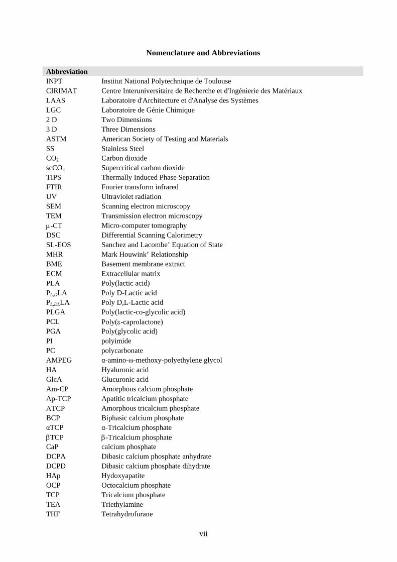
Nomenclature and Abbreviations Abbreviation INPT Institut National Polytechnique de Toulouse CIRIMAT Centre Interuniversitaire de Recherche et d'Ingénierie des Matériaux LAAS Laboratoire d'Architecture et d'Analyse des Systèmes LGC Laboratoire de Génie Chimique 2 D Two Dimensions 3 D Three Dimensions ASTM American Society of Testing and Materials SS Stainless Steel CO2 Carbon dioxide scCO2 Supercritical carbon dioxide TIPS Thermally Induced Phase Separation FTIR Fourier transform infrared UV Ultraviolet radiation SEM Scanning electron microscopy TEM Transmission electron microscopy -CT Micro-computer tomography DSC Differential Scanning Calorimetry SL-EOS Sanchez and Lacombe’ Equation of State MHR Mark Houwink’ Relationship BME Basement membrane extract ECM Extracellular matrix PLA Poly(lactic acid) PL,DLA Poly D-Lactic acid PL,DLLA Poly D,L-Lactic acid PLGA Poly(lactic-co-glycolic acid) PCL Poly(-caprolactone) PGA Poly(glycolic acid) PI polyimide PC polycarbonate AMPEG α-amino-ω-methoxy-polyethylene glycol HA Hyaluronic acid GlcA Glucuronic acid Am-CP Amorphous calcium phosphate Ap-TCP Apatitic tricalcium phosphate TCP Amorphous tricalcium phosphate BCP Biphasic calcium phosphate αTCP α-Tricalcium phosphate TCP -Tricalcium phosphate CaP calcium phosphate DCPA Dibasic calcium phosphate anhydrate DCPD Dibasic calcium phosphate dihydrate HAp Hydoxyapatite OCP Octocalcium phosphate TCP Tricalcium phosphate TEA Triethylamine THF Tetrahydrofurane
viii
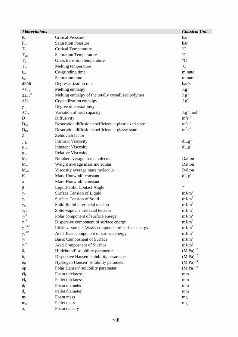
Abbreviations Classical Unit Pc Critical Pressure bar Psat Saturation Pressure bar Tc Critical Temperature oC Tsat Saturation Temperature oC Tg Glass transition temperature °C Tm Melting temperature C tco Co-grinding time minute tsat Saturation time minute dP/dt Depressurization rate bar/s m Melting enthalpy J.g-1 m
Melting enthalpy of the totally cystallised polymer J.g-1 c Crystallization enthalpy J.g-1 Degree of crystallinity Cp Variation of heat capacity J.g-1.mol-1 D Diffusivity m2s-1 Ddg Desorption diffusion coefficient at plasticized state m2s-1 Ddp Desorption diffusion coefficient at glassy state m2s-1 Z Zeldovich factor Intrinsic Viscosity dL.g-1 inh Inherent Viscosity dL.g-1 rel Relative Viscosity Mn Number average mass molecular Dalton Mw Weight average mass molecular Dalton Mvis Viscosity average mass molecular Dalton K Mark Houwink’ constant dL.g-1 a Mark Houwink’ constant Liquid-Solid Contact Angle ° γL Surface Tension of Liquid mJ/m2 γS Surface Tension of Solid mJ/m2 γSL Solid-liquid interfacial tension mJ/m2 γSV Solid-vapour interfacial tension mJ/m2 γS
p Polar component of surface energy mJ/m2 γS
d Dispersive component of surface energy mJ/m2 S
LW Lifshitz–van der Waals component of surface energy mJ/m2 S
AB Acid–Base component of surface energy mJ/m2 γS
− Basic Composnent of Surface mJ/m2 γS
+ Acid Composnent of Surface mJ/m2 δt Hildebrand’ solubility parameter (M Pa)1/2 δd Dispersive Hansen’ solubility parameter (M Pa)1/2 δH Hydrogen Hansen’ solubility parameter (M Pa)1/2 δp Polar Hansen’ solubility parameter (M Pa)1/2 Øf Foam thickness mm Øp Pellet thickness mm df Foam diameter mm dp Pellet diameter mm mf Foam mass mg mp Pellet mass mg f Foam density
ix
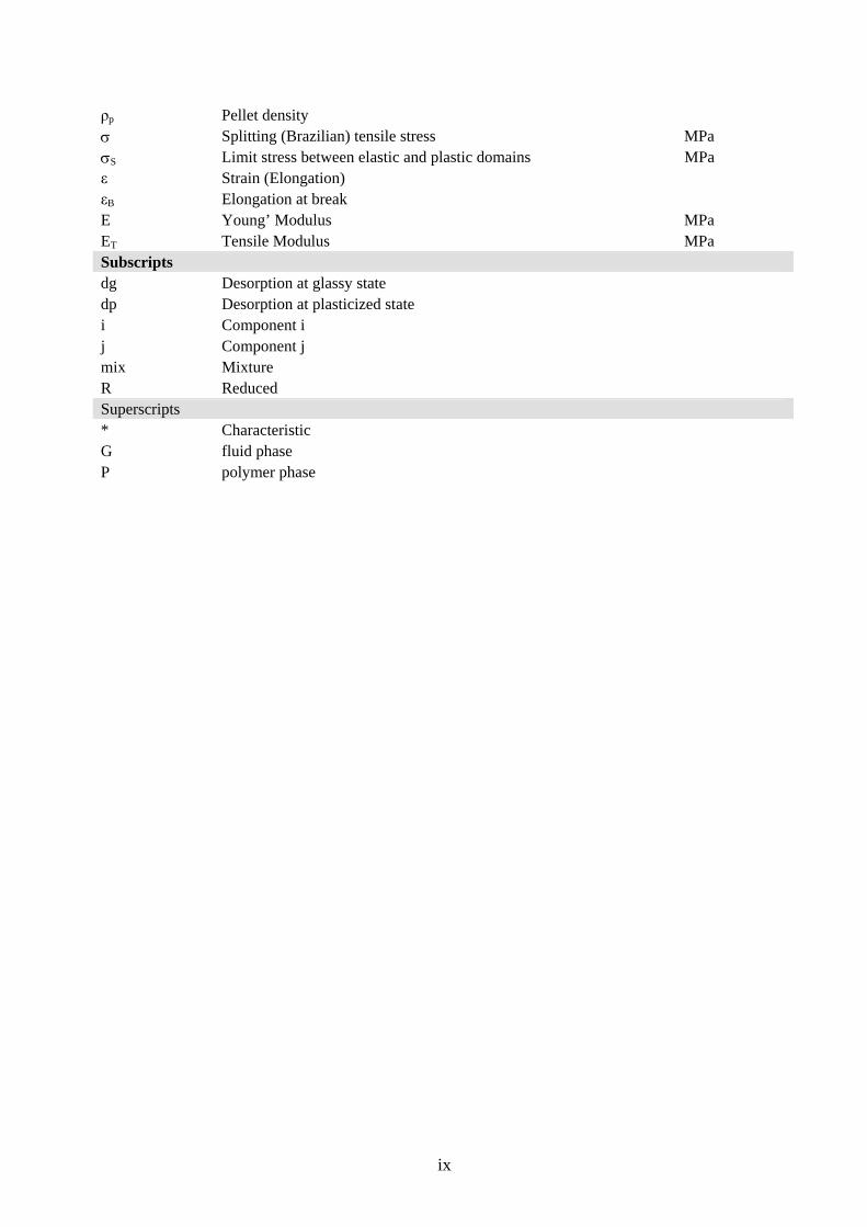
ρp Pellet density Splitting (Brazilian) tensile stress MPa S Limit stress between elastic and plastic domains MPa ε Strain (Elongation) εB Elongation at break E Young’ Modulus MPa ET Tensile Modulus MPa Subscripts dg Desorption at glassy state dp Desorption at plasticized state i Component i j Component j mix Mixture R Reduced Superscripts * Characteristic G fluid phase P polymer phase

x
- xi -
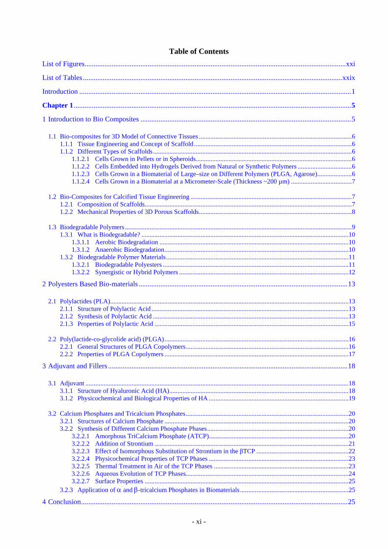
Table of Contents
List of Figures ................................................................................................................................................. xxi
List of Tables ................................................................................................................................................ xxix
Introduction ....................................................................................................................................................... 1
Chapter 1 .......................................................................................................................................................... 5
1 Introduction to Bio Composites ..................................................................................................................... 5
1.1 Bio-composites for 3D Model of Connective Tissues ............................................................................................. 6 1.1.1 Tissue Engineering and Concept of Scaffold ................................................................................................ 6 1.1.2 Different Types of Scaffolds ......................................................................................................................... 6
1.1.2.1 Cells Grown in Pellets or in Spheroids ............................................................................................... 6 1.1.2.2 Cells Embedded into Hydrogels Derived from Natural or Synthetic Polymers ................................. 6 1.1.2.3 Cells Grown in a Biomaterial of Large–size on Different Polymers (PLGA, Agarose) ..................... 6 1.1.2.4 Cells Grown in a Biomaterial at a Micrometer-Scale (Thickness ~200 µm) ..................................... 7
1.2 Bio-Composites for Calcified Tissue Engineering .................................................................................................. 7 1.2.1 Composition of Scaffolds .............................................................................................................................. 7 1.2.2 Mechanical Properties of 3D Porous Scaffolds ............................................................................................. 8
1.3 Biodegradable Polymers .......................................................................................................................................... 9 1.3.1 What is Biodegradable? .............................................................................................................................. 10
1.3.1.1 Aerobic Biodegradation ................................................................................................................... 10 1.3.1.2 Anaerobic Biodegradation ................................................................................................................ 10
1.3.2 Biodegradable Polymer Materials ............................................................................................................... 11 1.3.2.1 Biodegradable Polyesters ................................................................................................................. 11 1.3.2.2 Synergistic or Hybrid Polymers ....................................................................................................... 12
2 Polyesters Based Bio-materials .................................................................................................................... 13
2.1 Polylactides (PLA) ................................................................................................................................................. 13 2.1.1 Structure of Polylactic Acid ........................................................................................................................ 13 2.1.2 Synthesis of Polylactic Acid ....................................................................................................................... 13 2.1.3 Properties of Polylactic Acid ...................................................................................................................... 15
2.2 Poly(lactide-co-glycolide acid) (PLGA) ................................................................................................................ 16 2.2.1 General Structures of PLGA Copolymers ................................................................................................... 16 2.2.2 Properties of PLGA Copolymers ................................................................................................................ 17
3 Adjuvant and Fillers ..................................................................................................................................... 18
3.1 Adjuvant ................................................................................................................................................................ 18 3.1.1 Structure of Hyaluronic Acid (HA) ............................................................................................................. 18 3.1.2 Physicochemical and Biological Properties of HA ..................................................................................... 19
3.2 Calcium Phosphates and Tricalcium Phosphates ................................................................................................... 20 3.2.1 Structures of Calcium Phosphate ................................................................................................................ 20 3.2.2 Synthesis of Different Calcium Phosphate Phases ...................................................................................... 20
3.2.2.1 Amorphous TriCalcium Phosphate (ATCP) ..................................................................................... 20 3.2.2.2 Addition of Strontium ...................................................................................................................... 21 3.2.2.3 Effect of Isomorphous Substitution of Strontium in the βTCP ........................................................ 22 3.2.2.4 Physicochemical Properties of TCP Phases ..................................................................................... 23 3.2.2.5 Thermal Treatment in Air of the TCP Phases .................................................................................. 23 3.2.2.6 Aqueous Evolution of TCP Phases ................................................................................................... 24 3.2.2.7 Surface Properties ............................................................................................................................ 25
3.2.3 Application of and -tricalcium Phosphates in Biomaterials .................................................................. 25
4 Conclusion .................................................................................................................................................... 25
- xii -
Chapter 2 ........................................................................................................................................................ 27
1 Generalities on Polymer Foams .................................................................................................................... 27
2 Manufacturing of Porous Materials by Wet Methods .................................................................................. 28
2.1 Solvent Casting/Particulate Leaching .................................................................................................................... 28
2.2 Ice Particle-Leaching ............................................................................................................................................. 29
2.3 Gas-Foaming/Salt-Leaching Technique ................................................................................................................ 30
2.4 Gel-Pressing Technique ......................................................................................................................................... 31
2.5 PLGA Microspheres for Tissue-Engineered Scaffold ........................................................................................... 32
2.6 Particle-Aggregated Scaffolds Technique ............................................................................................................. 33
2.7 Freeze-Drying Method .......................................................................................................................................... 33
2.8 Thermally Induced Phase Separation (TIPS) Technique ....................................................................................... 34
2.9 Centrifugation Method .......................................................................................................................................... 35
2.10 Injectable Thermosensitive Gel Technique ........................................................................................................... 36
2.11 Liquid-Liquid Phase Separation Technique .......................................................................................................... 37
2.12 Solid-Liquid Phase Separation Technique ............................................................................................................. 38
2.13 Fibre Mesh/Fibre Bondong Technique .................................................................................................................. 38
2.14 Hydrocarbon Templating Technique ..................................................................................................................... 38
2.15 Microspheres Bonding Technique ......................................................................................................................... 39
2.16 Rapid Prototyping Techniques .............................................................................................................................. 39 2.16.1 Three Dimensional Printing (3 DP) ............................................................................................................ 40 2.16.2 Stereolithography (SLA)............................................................................................................................. 40
2.17 Other Derivated Techniques .................................................................................................................................. 41 2.17.1 Combination of Leaching of a Fugitive Phase and Polymer Precipitation ................................................. 41 2.17.2 Phase-Change Jet Printing .......................................................................................................................... 42
3 Polymer Processing by Supercritical Fluids ................................................................................................. 42
3.1 Bases on Supercritical Fluids ................................................................................................................................ 42
3.2 Basic Techniques in Supercritical Fluids Technology .......................................................................................... 44
3.3 Scaffolds Prepared by Phase Inversion using scCO2 as Anti-solvent .................................................................... 45
3.4 Scaffolds Prepared by scCO2 Foaming ................................................................................................................. 46
4 Theoretical Background of Gas Foaming ..................................................................................................... 48
4.1 Diffusion ................................................................................................................................................................ 48
4.2 Plasticization of Polymers by CO2 ........................................................................................................................ 51
4.3 Nucleation ............................................................................................................................................................. 53
- xiii -
4.4 Distribution of Pores .............................................................................................................................................. 54
5 Manufacturing of the Composite Biomaterials ............................................................................................ 56
5.1 Fundements of Co-grinding Process ...................................................................................................................... 56 5.1.1 Mechanism of Size Reduction .................................................................................................................... 56 5.1.2 Fragmentation Mechanisms ........................................................................................................................ 57 5.1.3 Agglomeration Phenomena ......................................................................................................................... 57
5.2 Obtention of Composites by the Co-grinding Process ........................................................................................... 58
6 Conclusion .................................................................................................................................................... 60
Chapter 3 ........................................................................................................................................................ 61
1 Differential Scanning Calorimetry (DSC) .................................................................................................... 61
1.1 Generalities on Thermal Transitions of Polymers ................................................................................................. 61
1.2 First Order Transitions ........................................................................................................................................... 62
1.3 Second Order Transition ........................................................................................................................................ 63
2 Intrinsic Viscosity ........................................................................................................................................ 64
2.1 Molecular Mass of Polymer and Viscosity ............................................................................................................ 64
2.2 General Principle of Viscosity Measurement ........................................................................................................ 64
2.3 The Mark-Houwink Relationship (MHR).............................................................................................................. 66
2.4 The Mark-Houwink Constants of Polylactides and Hyaluronic Acid .................................................................... 66
3 Laser Granulometry Method ........................................................................................................................ 67
3.1 Granulometry ......................................................................................................................................................... 67
3.2 Principle of Laser Analysis .................................................................................................................................... 67 3.2.1 Rayleigh’ Theory ........................................................................................................................................ 68 3.2.2 Lorenz-Mie’ Theory .................................................................................................................................... 68 3.2.3 Fraunhofer’ Theory ..................................................................................................................................... 69
4 Sorption Analysis ......................................................................................................................................... 70
5 Microscopic Methods to Analyze Porous Structures ................................................................................... 70
5.1 Methods to Determine Porosity ............................................................................................................................. 70 5.1.1 Geometric Porosity ..................................................................................................................................... 70 5.1.2 Mercury Porosimetry .................................................................................................................................. 71 5.1.3 X-ray Microtomography ............................................................................................................................. 72
5.2 Scanning Electron Microscopy Observations ........................................................................................................ 72 5.2.1 Bases of Image Analysis ............................................................................................................................. 73 5.2.2 Morphological Filtering .............................................................................................................................. 74
6 Macroscopic Methods .................................................................................................................................. 75
6.1 Mechanical Brazilian Tests .................................................................................................................................... 75 6.1.1 Principle of the Test .................................................................................................................................... 75 6.1.2 Compression of Porous Materials ............................................................................................................... 76
6.2 Surface Energy Experiments ................................................................................................................................. 77
- xiv -
6.2.1 Surface Tensions of Liquids ....................................................................................................................... 78 6.2.1.1 Du Noüy Ring Method ..................................................................................................................... 79 6.2.1.2 Wilhelmy Plate Method ................................................................................................................... 79 6.2.1.3 Lucas-Washburn’ Method ................................................................................................................ 80 6.2.1.4 Surface Tensions of Classical Liquids ............................................................................................. 80
6.2.2 Surface Energy of Solids ............................................................................................................................ 80 6.2.2.1 Young-Dupré’ Equation ................................................................................................................... 80 6.2.2.2 Model of Owens-Wendt : Two Components Theory ....................................................................... 81 6.2.2.3 Model of Good-Van Oss : Three Components Theory .................................................................... 83
7 Designs of Experiments ................................................................................................................................ 84
7.1 Modelization Plans: Doehlert’s Design ................................................................................................................. 84
7.2 Screening Plans: Taguchi’ Design ......................................................................................................................... 85
8 Conclusion .................................................................................................................................................... 86
Chapter 4 ........................................................................................................................................................ 87
1 Procedure for Size Reduction ....................................................................................................................... 87
1.1 Size Reduction ....................................................................................................................................................... 87 1.1.1 Size Reduction by Knife Mill ..................................................................................................................... 87 1.1.2 Tumbling Ball Mill Grinding ...................................................................................................................... 88
1.2 Sieving of Ground Material ................................................................................................................................... 89
1.3 Mixing of Polymer Powder with Fillers ................................................................................................................ 89 1.3.1 Simple Mixing of Polymer Powder with Fillers ......................................................................................... 90 1.3.2 Co-grinding in the Tumbling Ball Mill ....................................................................................................... 90
1.4 Preparation of Pellets by Dry Method ................................................................................................................... 91 1.4.1 Evacuable Pellet Die ................................................................................................................................... 91 1.4.2 Procedure to Prepare Pellets ....................................................................................................................... 92
1.4.2.1 Preparation of the Die ...................................................................................................................... 93 1.4.2.2 Loading the Die ................................................................................................................................ 93 1.4.2.3 Processing the Pellets ....................................................................................................................... 93 1.4.2.4 Removing the Pellets ....................................................................................................................... 93
1.5 Preparation of Pellets by Wet Method ................................................................................................................... 93
2 ScCO2 Foaming Process ............................................................................................................................... 94
2.1 SEPAREXTM SF200 scCO2 Pilot Plant ................................................................................................................. 94 2.1.1 Experimental Device .................................................................................................................................. 94 2.1.2 Setup One: Filling the Chamber with Teflon® ............................................................................................ 96 2.1.3 Setup Two: Filling the Chamber with Glass Beads .................................................................................... 96
2.2 SEPAREX SFC6 scCO2 Laboratory Plant ........................................................................................................ 96 2.2.1 Experimental Device .................................................................................................................................. 96 2.2.2 Experimental Procedure .............................................................................................................................. 96
2.2.2.1 Initial Filling of Chamber with CO2 ................................................................................................. 97 2.2.2.2 Variations of Saturation Pressure and Temperature Holding For Time t ......................................... 98 2.2.2.3 Depressurization of CO2 .................................................................................................................. 98
3 Protocols for Analysis .................................................................................................................................. 99
3.1 Granulometry ......................................................................................................................................................... 99
3.2 Differential Scanning Calorimetry ...................................................................................................................... 100
- xv -
3.3 Contact Angle Measurement ............................................................................................................................... 101
4 Protocols for Porosity and Pore Size Measurement ................................................................................... 102
4.1 Average Geometric Porosity ................................................................................................................................ 102
4.2 2D Image Analysis .............................................................................................................................................. 103 4.2.1 Sputter Coater ........................................................................................................................................... 103 4.2.2 SCION Image Analysis .......................................................................................................................... 104
4.3 3D Hg Intrusion Porosity ..................................................................................................................................... 107
4.4 3D Micro Computer Tomography ....................................................................................................................... 108 4.4.1 Acquisition ................................................................................................................................................ 109 4.4.2 Corrections ................................................................................................................................................ 109 4.4.3 Reconstruction .......................................................................................................................................... 109 4.4.4 Viewing Results ........................................................................................................................................ 109 4.4.5 Wide Variety of Post Processing ............................................................................................................... 109
5 Mechanical Tests on Foams ....................................................................................................................... 110
5.1 Experimental Conditions of Test ......................................................................................................................... 110
5.2 Principle of Curve Analysis ................................................................................................................................. 110
6 Conclusion .................................................................................................................................................. 111
Chapter 5 ...................................................................................................................................................... 112
1 Characterization of Biomaterials ................................................................................................................ 113
1.1 Characterization of Polylactide Powders ............................................................................................................. 113 1.1.1 Experiments on Polylactide Powders by Viscosimetry. ............................................................................ 115 1.1.2 Discussion on the Molecular Mass ........................................................................................................... 116 1.1.3 Characterization of Polylactide Powders by DSC ..................................................................................... 116 1.1.4 Discussion on the Transitions ................................................................................................................... 118
1.1.4.1 Effect of L and DL Ratio on Thermal Property of Polylactide Acid .............................................. 118 1.1.4.2 Effect of LA/GA Ratio on Tg of Polylactides ................................................................................. 119
1.2 Characterization of Biomaterials Pellets .............................................................................................................. 119 1.2.1 Mechanical Experiments ........................................................................................................................... 119 1.2.2 Discussion on Mechanical Modulus ......................................................................................................... 119
2 Kinematics and Thermodynamics Experiments ......................................................................................... 120
2.1 Sorption-Diffusion Kinetics ................................................................................................................................. 120
2.2 Desorption-Diffusion Kinetics ............................................................................................................................. 121
2.3 The Sorption Isotherm ......................................................................................................................................... 123 3.1.2 Discussion on the Blends of PL,DLLA and PLGA50:50 ................................................................................ 125 3.1.3 PL,DLLA and PLGA85:15 Blend ................................................................................................................... 125 3.1.4 Discussion on the Blends of PL,DLLA and PLGA85:15 ................................................................................ 126
3.2 Influence of the Parameters of the scCO2 Process ............................................................................................... 126 3.2.1 Model with a 24 Complete Design ............................................................................................................. 126 3.2.2 Model with a Taguchi’ Design for PLGA50:50 Foaming ............................................................................ 128 3.2.3 Model with a Doehlert’ Design for PLGA50:50 Foaming ........................................................................... 130
3.2.3.1 Experiments with a Doehlert’ Design ............................................................................................ 130 3.2.3.2 Discussion on the Effect of the Various CO2 Process Parameters .................................................. 132
4 Factors Affecting on Pores Size and Porosity ............................................................................................ 135
- xvi -
4.1 Effect of the Polymer Composition ..................................................................................................................... 135
4.2 Effect of Depressurization Rates ......................................................................................................................... 135
4.3 Effect of Saturation Pressure (Psat) ...................................................................................................................... 137
4.4 Effect of Saturation Temperature (Tsat) ............................................................................................................... 138
4.5 Effect of Saturation Time (tsat) ............................................................................................................................. 139
4.6 Effect of the dP/dt and dT/dt ............................................................................................................................... 139
4.7 Effect of the Geometry of the Pressure Chamber ................................................................................................ 140
4.8 Interconnectivity and Coalescence Behaviour of the Scaffolds........................................................................... 141
4.9 Influence of Pellet Thickness on Foaming .......................................................................................................... 142 4.9.1 Porosity and Cell Density ......................................................................................................................... 142 4.9.2 Pores Size Distribution ............................................................................................................................. 143 4.9.3 Correlation Between Effects of Pellet Thickness and Process Parameters ............................................... 143
4.10 Discussion on Foam Morphology ........................................................................................................................ 144
5 Conclusion .................................................................................................................................................. 146
Chapter 6 ...................................................................................................................................................... 147
1 Optimization of PLA’s Foams Processed by Wet and Dry Methods ......................................................... 147
1.1 Experimental Procedure ...................................................................................................................................... 147 1.1.1 Preparation of Pellets by Wet and Dry Methods ....................................................................................... 147 1.1.2 Taguchi’ Design for Foaming ................................................................................................................... 148
1.2 PL,DLA Foams Processed by Wet and Dry Methods: Initial Taguchi Plan .......................................................... 148 1.2.1 Effect of Process Parameters on Equivalent Pore Diameter (de) .............................................................. 150 1.2.2 Effect of Process Parameters on Geometric Porosity ............................................................................... 150
1.3 PL,DLA Foams Processed by Wet and Dry Methods: Complementary Taguchi’ Plan ......................................... 151 1.3.1 Effect of Process Parameters on Equivalent Pore Diameter (de) .............................................................. 153 1.3.2 Effect of Process Parameters on Geometric Porosity ............................................................................... 153
1.4 PL,DLLA Foams Processed by Wet and Dry Methods: Initial Taguchi Plan ......................................................... 154 1.4.1 Effect of Process Parameters on Equivalent Pore Diameter (de) .............................................................. 155 1.4.2 Effect of Process Parameters on Geometric Porosity ............................................................................... 156
1.5 PL,DLLA Foams Processed by Wet and Dry Methods: Complementary Taguchi’ Plan ....................................... 156 1.5.1 Effect of Process Parameters on Equivalent pore diameter (de) ................................................................ 158 1.5.2 Effect of Process Parameters on Geometric Porosity ............................................................................... 158
1.6 Comparison Between Both PLAs ........................................................................................................................ 159
2 Optimization of PLGA’s Foams by Wet and Dry Method. ........................................................................ 161
2.1 PLGA50:50 Foams Processed by Wet and Dry Methods ....................................................................................... 161 2.1.1 Effect of Process Parameters on Equivalent Pore Diameter (de) .............................................................. 162 2.1.2 Effect of Process Parameters on Geometric Porosity ............................................................................... 163
2.2 PLGA50:50 Foams by Wet and Dry Methods by Complementary Taguchi’ Plan ................................................. 163 2.2.1 Effect of Process Parameters on Equivalent Pore Diameter (de) .............................................................. 165 2.2.2 Effect of Process Parameters on Geometric Porosity ............................................................................... 165
- xvii -
2.3 PLGA85:15 Foams Processed by Wet and Dry Methods: Initial Taguchi’ Plan .................................................... 166 2.3.1 Effect of Process Parameters on Equivalent Pore Diameter (de) ............................................................... 167 2.3.2 Effect of Process Parameters on Geometric Porosity ................................................................................ 168
2.4 PLGA85:15 Foams by Wet and Dry Methods by Complementary Taguchi Plan .................................................. 169 2.4.1 Effect of Process Parameters on Equivalent Pore Diameter (de) ............................................................... 170 2.4.2 Effect of Process Parameters on Geometric Porosity ................................................................................ 171
2.5 Comparison Between Both PLGAs ..................................................................................................................... 171
2.6 Pore Morphology and Anisotropy of Foams by Both Methods ........................................................................... 173
2.7 Interconnectivity of Pores in Foams by Both Methods ........................................................................................ 176
2.8 Mechanical Properties of the Foams by Wet and Dry Methods .......................................................................... 178
2.9 General Discussion .............................................................................................................................................. 178
3 Modification of the Surface by Adding Hyaluronic Acid .......................................................................... 179
3.1 Granulometry Analysis of PLGA and HA Before and After Co-grinding ........................................................... 179
3.2 Contact Angle Measurement and Surface Energy on Pellets ............................................................................... 181 3.2.1 Results ....................................................................................................................................................... 181
3.2.1.1 Contact Angles with Water and Pellets of PLGA, HA and PLGA/HA Blends .............................. 181 3.2.1.2 Surface Energy of PLGA, HA and PLGA/HA blends ................................................................... 182
3.2.2 Origin of the Increase of Surface Energy .................................................................................................. 183
4 Foams of PLGA85:15/HA Blends ................................................................................................................. 185
4.1 Preparation of Pellets ........................................................................................................................................... 185
4.2 Effect of scCO2 Parameters on the Microstucture of Foams ............................................................................... 185 4.2.1 Effect of Depressurization Rate on the Microstucture of Foams .............................................................. 185 4.2.2 Effect of Saturation Temperature on the Microstucture of Foams ............................................................ 187
5 General Discussion ..................................................................................................................................... 188
6 Conclusion .................................................................................................................................................. 189
Chapter 7 ...................................................................................................................................................... 190
1 Characterization of Composites ................................................................................................................. 190
1.1 Fillers and Adjuvant ............................................................................................................................................ 190 1.1.1 Sr Calcium Phosphate ............................................................................................................................... 191
1.1.1.1 Synthesis and Characterization of Calcium Phophates .................................................................. 191 1.1.1.2 Calcium Phosphate Characterization .............................................................................................. 191 1.1.1.3 Calcium Phosphate Granulometry .................................................................................................. 193
1.2 Adjuvant: Porogen Agent .................................................................................................................................... 194 1.2.1 Industrial Waxes ....................................................................................................................................... 194 1.2.2 Thermal Degradation ................................................................................................................................ 195
2 Experiments on Polylactides/Tri-calcium Phosphate Scaffolds ................................................................. 195
2.2 Experiments on Polylactides/Tri-calcium Phosphate ........................................................................................... 195
2.3 Analysis of Experiments on Polylactides/Tri-calcium Phosphate ....................................................................... 197
3 Foams of Polylactides/Calcium Phosphates Blends and Composites ........................................................ 198
- xviii -
3.2 Experiments on PLA/Waxes Scaffolds ............................................................................................................... 198 3.2.1 Preliminary Experimentation with Wax as Porogen Agent ...................................................................... 198 3.2.2 SEM Analysis of Foams ........................................................................................................................... 199 3.2.3 Effect of Wax on the Equivalent Pore Size and Geometric Porosity ........................................................ 201
3.3 Experiments on Polylactides/Tri-Calcium Phosphate/Wax Scaffolds ................................................................. 203 3.3.1 Effect of the Ratio of Wax on the Geometric Porosity and Equivalent Pore Size .................................... 203 3.3.2 Effect of Co-grinding Filler and PLGA on the Pore Morphology ............................................................ 205
3.4 Complementary Experiments on PLGA85:15/Tri-calcium Phosphate/Wax Scaffolds .......................................... 206
4 Conclusion .................................................................................................................................................. 209
Chapter 8 ...................................................................................................................................................... 210
1 Semi-industrial Production of Bone Scaffolds ........................................................................................... 210
1.1 Matrix: Polylactides............................................................................................................................................. 211 1.1.1 Experiments with Different Polylactides .................................................................................................. 211 1.1.2 Polylactide with Higher D,L Contents ...................................................................................................... 212
1.2 Effect of Polymer Particle Size on Foaming ....................................................................................................... 213 1.2.1 Foaming of PLGA85:15 with Different Particle Size .................................................................................. 214
2 Filler: Tri-calcium phosphate Doped by Sr ................................................................................................ 215
2.1 Experimentation on Blends and Composite Foams ............................................................................................. 215 2.1.1 Experimentation on Composite Foaming with Different Co-grinding Times .......................................... 216 2.1.2 Foaming of Fine Powder and Filler Blend by Simple Mixing .................................................................. 217 2.1.3 Mixing Experimentation on Composite Foaming with Different Polymer Particle Size .......................... 218
3 Process Control for Composite Foaming .................................................................................................... 220
3.1 Semi-Industrial Foaming ..................................................................................................................................... 220 3.1.1 Pellet Positions in scCO2 Chamber ........................................................................................................... 220
3.2 Final Experiments ................................................................................................................................................ 222 3.2.1 Multi Pellet Formation in a Batch and Effect on Foaming ....................................................................... 222 3.2.2 Preparation of Foams ................................................................................................................................ 224
3.2.2.1 Filling, Soaking and Depressurization Time of CO2 in Chamber .................................................. 224 3.2.2.2 Temperature Variation During Soaking of CO2 ............................................................................. 224 3.2.2.3 Dual Depressurization Rate............................................................................................................ 225 3.2.2.4 Temperature Variation During Depressurization of CO2 ............................................................... 225 3.2.2.5 Retention Time after the Depressurization Step ............................................................................. 225
3.2.3 Final foam experiments ............................................................................................................................ 225 3.2.4 Discussion on the Rugdness of the Process .............................................................................................. 226
4 Mechanical Properties of Scaffolds ............................................................................................................ 229
4.1 Mechanical Characteristics of PLGA85:15 Foam .................................................................................................. 229
4.2 Compressive Properties of Optimized PLGA85:15 Composite Foams .................................................................. 231
4.3 Co-grinding time Effect on Compressive Properties of Composite Foams ......................................................... 231
4.4 Effect of Different Fillers and Wax-A Ratio on Compressive Properties of PLGA85:15 Composite Foam .......... 232
5 Interconnectivity of Pores by CT ............................................................................................................ 233
5.1 PLGA85:15 Scaffold .............................................................................................................................................. 233
5.2 PLGA85:15 Composite Scaffold ............................................................................................................................ 235

- xix -
6 General Discussion ..................................................................................................................................... 236
7 Conclusion .................................................................................................................................................. 237
General Conclusion and Perspective ............................................................................................................. 238
BIBLIOGRAPPHY ....................................................................................................................................... 242
ANNEXES .................................................................................................................................................... 264
Annex-A-1 ..................................................................................................................................................... 266
Annex A-2 ..................................................................................................................................................... 270
Annex A-3 ..................................................................................................................................................... 271

xx
- xxi -
List of Figures Figure 1.1: Structures of selected biodegradable polymers ............................................................................. 12 Figure 1.2: Stereo-forms of lactides. ............................................................................................................... 13 Figure 1.3: Ring opening polymerization of lactide to polylactide. ................................................................ 14 Figure 1.4: Different ways of producing PLA. ................................................................................................ 14 Figure 1.5: Schemaic synthesis of poly(lactide-co-glycolide). ........................................................................ 17 Figure 1.6: Electron micrograph and chemical HA structure. ......................................................................... 19
Figure 2.1: Procedure of solvent casting/particulate leaching. ........................................................................ 29 Figure 2.2: Procedure of ice particle–leaching. ............................................................................................... 30 Figure 2.3: Procedure of gas foaming/salt-leaching method. .......................................................................... 31 Figure 2.4: Procedure of scaffolds by gel-pressing method. ........................................................................... 32 Figure 2.5: Schematic procedure of the processing of PLGA microsphere scaffolds. .................................... 33 Figure 2.6: Schematic procedure for manufacturing of scaffolds with the particle-aggregated technique. .... 33 Figure 2.7: Schematic preparation processing of scaffold by the freeze-drying method. ............................... 34 Figure 2.8: Schematic preparation processing of thermally induced phase separation method. ..................... 35 Figure 2.9: Schematic procedure showing the fabrication of scaffolds by centrifugation method and
photographs of variously shaped scaffolds. ................................................................................. 36 Figure 2.10: Reaction of injectable thermosensitive gel.................................................................................. 37 Figure 2.11: Schematic stepwise representation of the polymeric foaming using hydrocarbon porogen. ...... 39 Figure 2.12: Schematic diagram of the fused deposition modelling (FDM) system. ...................................... 40 Figure 2.13: Schematic diagram of the 3D BioplotterTM system. .................................................................... 40 Figure 2.14: Schematic diagram of the Stereolithography (SLA) system. ...................................................... 41 Figure 2.15: Schematic diagram of the phase change jet printing system, the Model-Maker II. .................... 42
Figure 2.16: Phase diagrams P-T and -P for a pure CO2. .............................................................................. 43
Figure 2.17: ScCO2 experimental apparatus (A) CO2 tank, (B) syringe pump and (C) pressure vessel. ........ 45 Figure 2.18: Schematic representation of the supercritical fluid foaming process. ......................................... 46 Figure 2.19: Schematic presentation for scaffold generation during scCO2 foaming. .................................... 47 Figure 2.20: Evolution of process parameters and the occurring phenomena during the foaming with time. 48 Figure 2.21: Schematic of the phenomenon of fragmentation in the co-grinding. .......................................... 59 Figure 2.22: Different stages of agglomeration during the co-grinding: (a) adhesion, (b) coating and (c)
agglomeration. ............................................................................................................................. 59
Figure 3.1: Differential scanning calorimetry. ................................................................................................ 62 Figure 3.2: Thermograms of two PLLAs of different Mw. .............................................................................. 63 Figure 3.3: Characteristic variation of glass transition in PLGA. ................................................................... 63 Figure 3.4: Schematic representation of the Ubbelohde viscosimeter. ............................................................ 65 Figure 3.5: Variation with concentration of reduced specific and inherent viscosities of PL,DLA (LR 704). .. 66
Figure 3.6: (A) Mastersizer 2000 (Malvern Instruments) (B) Schematic diagram showing the main
components of a laser diffraction particle size analyzer. ............................................................. 67 Figure 3.7: Scheme of laser diffraction of a spherical particle. ....................................................................... 68 Figure 3.8: Three dimensional model of scattering from a dipole. .................................................................. 68 Figure 3.9: Scattering patterns of two particles of a different size. ................................................................. 69 Figure 3.10: Principles of Fresnel’ diffraction (A) and Fraunhofer’ diffraction (B and C). ............................ 69 Figure 3.11: Desorption of CO2 from PLGA50:50 with time. ............................................................................ 70
- xxii -
Figure 3.12: (A): Hg porosimeter apparatus and (B): Pore size distribution of PLLA samples. ...................... 71
Figure 3.13: CT principle and images of PLLA/Silica sample. ..................................................................... 72
Figure 3.14: Schematic representation of interactions beam on specimen surface. ......................................... 73 Figure 3.15: SCION® Image processing and pore data retrieval. .................................................................... 74 Figure 3.16: (A): A binary image and a structuring element (top left corner).(B): Erosion (C): Dilation (D):
Opening (E): Closing of the original image. ................................................................................ 74 Figure 3.17: H25KS Brazilian testing equipment. ........................................................................................... 75 Figure 3.18: (A): Principle, (B): Load geometry, (C): Simulation and (D): Cleavage of a Brazilian disk test.
...................................................................................................................................................... 76 Figure 3.19: Compression testing equipment for foams and result. ................................................................ 77 Figure 3.20: Wetting of hydrophilic and hydrophobic samples. ...................................................................... 78 Figure 3.21: The Du Noüy’ ring method. ........................................................................................................ 79 Figure 3.22: The Wilhelmy’ plate method with a platinum plate. ................................................................... 79 Figure 3.23: Principle of the absorption Wasburn’ method. ............................................................................ 80 Figure 3.24: Vectorial equilibrium for a drop of a liquid resting on a solid surface to balance three forces. . 81 Figure 3.25: Example of determination of surface energy components of a blend PLGA + 5 % HA ............. 83 Figure 3.26: Example of determining the surface energy components with Good-Van Oss’ method ............ 84 Figure 3.27: Distribution of experimental points for a Doehlert’s design of 2-variables. ............................... 85
Figure 4.1: Polylactide granulates size reduction by knife mill. ...................................................................... 88 Figure 4.2: Milling process in tumbling ball mill. ........................................................................................... 88 Figure 4.3: Cataract movement of grinding media. ......................................................................................... 89 Figure 4.4: AFNOR and ASTM 3 ½ in diameter sieves. ................................................................................. 90 Figure 4.5: Magnetic stirrer mixing for composite materials. ......................................................................... 90 Figure 4.6: Multistep size reduction of composite. .......................................................................................... 91 Figure 4.7: Schematic diagram to produce pellets in semi-industrial quantities. ............................................ 92 Figure 4.8: Schematic representation to process pellets by using hydraulic press. ......................................... 92 Figure 4.9: Schematic representation of processing pellets by wet method. ................................................... 94
Figure 4.10: SEPAREX Pilot SF200 Process Flow Diagram. ..................................................................... 95
Figure 4.11: Details of equipment (SEPAREX Pilot SF200). ..................................................................... 95
Figure 4.12: Schematic representation of the cross section of the supercritical CO2 ...................................... 96
Figure 4.13: Details of equipment (SEPAREX Pilot SFC-6). ..................................................................... 97
Figure 4.14: SEPAREX Pilot SFC-6 Process Flow Diagram. ..................................................................... 97
Figure 4.15: Variation of chamber temperature during 20 minutes of scCO2 process for PLGA50:50 foam. .... 98 Figure 4.16: Graph presenting the drop in pressure during 40 sec of depressurization step. .......................... 98 Figure 4.17: Size distribution of PL,DLA particle after 30 minutes of grinding ............................................... 99 Figure 4.18: Variation of Particle Diameter with Grinding time for PL,DLA ................................................... 99 Figure 4.19: DSC analysis flow sheet of polymer material and foam. .......................................................... 100 Figure 4.20: Goniometer GBX used for contact angle measurement. ........................................................... 101 Figure 4.21: (A): Schematic diagram and (B): Two methods for determining the contact angle. ................. 101 Figure 4.22: Sputter coating and SEM processing flow diagram. ................................................................. 103 Figure 4.23: SEM Images of cross sectional foam. ....................................................................................... 104 Figure 4.24: Various steps of transformation of SEM image by Scion®. ...................................................... 105 Figure 4.25: Graphs obtained from the initial data of SCION® image analysis. ........................................... 106 Figure 4.26: Pore distribution comparison in a foam with different aspects. ................................................ 107 Figure 4.27: Autopore analyzer for porosity.................................................................................................. 108
- xxiii -
Figure 4.28: Incremental Intrusion vs Pore size. ........................................................................................... 108
Figure 4.29: Set up of CT and Flow chart of CT measurement process. .................................................. 109
Figure 4.30: CT slice view from different direction for different bone scaffold presenting the
interconnectivity. ....................................................................................................................... 110 Figure 4.31: Stress strain graph of PLGA foam obtained showing the three regions. .................................. 111
Figure 5.1: Courbe size distribution of various PLAs after knife mill grinding. ........................................... 115 Figure 5.2: Thermograms of various PLAs. .................................................................................................. 116 Figure 5.3: Thermograms of PLGA50:50. ........................................................................................................ 117 Figure 5.4: Thermograms of 3 different PLGA85:15. ...................................................................................... 117 Figure 5.5: Stress strain curve obtained from Brazilian Test for PL,DLA (PAB RL 68). ............................... 119 Figure 5.6: (A)-Kinetics and modelling of the sorption of CO2 in PLGA50:50 at 125 bar and 36.5°C, (B)
Desorption of CO2 from PLGA50:50 of CO2 in PLGA50:50 at 125 bars and 36.5°C. .................... 121 Figure 5.7: Desorption of CO2 from PLGA50:50 after 100 and 200 bars, at Tsat = 36.5°C and tsat = 120 min. 122 Figure 5.8: Sorption isotherm of CO2 into PLGA50:50. ................................................................................... 123 Figure 5.9: The depression of PLGA50:50 Tg as a function of the weight fraction of sorbed CO2: (♦) 100 bars;
(●) 200 bars. ............................................................................................................................... 124 Figure 5.10: Micrographs of the PL,DLLA and PLGA50:50 blend scaffolds. .................................................... 125 Figure 5.11: Average pore diameter of polymer blends as a function of PL,DLLA ratio. ............................... 125 Figure 5.12: Average pore diameter of polymer blends as a function of PL,DLLA ratio. ............................... 126 Figure 5.13: Average pore diameter as a function of PLGA50:50 ratio in the PLGA50:50/PLGA85:15 blends. .. 128 Figure 5.14: Variation of foam porosity. ....................................................................................................... 130 Figure 5.15: Average pore diameters of PLGA50:50 scaffolds as a function of the process parameters. ........ 130 Figure 5.16: Micrographs of the cross-section of the foams processed at P = 125 bars. ............................... 131 Figure 5.17: Variation of the porosity of the foams as a function of depressurization rate. .......................... 132 Figure 5.18: Influence of dP/dt on the pore size of the foams processed at scCO2 condition Psat = 100 bars,
Tsat = 36.5°C and tsat = 60 min. ................................................................................................... 133 Figure 5.19: (A) Variation of pore diameter of the PLGA50:50 scaffolds as the function of Psat; (B) Variation
of the energy barrier for PLGA50:50-CO2 system. ....................................................................... 134 Figure 5.20: Tg-w diagram of the PL,DLA (---) and PLGA50:50 (—); (●) and (♦), are the weight fraction of
CO2 in PL,DLA and PLGA50:50 at 100 bars, respectively. The value for the weight fraction of PL,DLA at 100 bars and 35°C is taken from [Pini et al., 2008]. ................................................. 136
Figure 5.21: Micrographs of scaffolds processed at Psat = 200 bars; Tsat = 36.5°C, tsat = 20 min. and dP/dt = 20 bar /s. ..................................................................................................................................... 137
Figure 5.22: Micrographs revealing the effect of Psat on pore size. ............................................................... 138 Figure 5.23: Micrographs revealing the effect of Tsat on pore size. ............................................................... 138 Figure 5.24: Micrographs revealing the effect of tsat on pore size. ................................................................ 139 Figure 5.25: Micrographs revealing the effect of dP/dt and dT/dt on pore size. ........................................... 140 Figure 5.26: Representation of the effect of the geometry of the pressure chamber on the porous structure.
................................................................................................................................................... 140 Figure 5.27: Micrographs depicting coalescence and collapse of pores. ....................................................... 141 Figure 5.28: Porosity of PLGA50:50 foams for pellets with different initial thickness. .................................. 142 Figure 5.29: Pore density of PLGA50:50 foams with different initial pellet thickness. ................................... 142 Figure 5.30: PLGA50:50 foams obtained with different initial pellet thicknesses. .......................................... 143 Figure 5.31: Different distribution of pores in PLGA50:50 foams. .................................................................. 143 Figure 5.32: Variation in PLGA50:50 foams geometric porosity for different process parameters. ................ 144
- xxiv -
Figure 5.33: Distribution of pores at different process condition. ................................................................. 145 Figure 5.34: Cell densities of pores produced at different process condition. ............................................... 145 Figure 5.35: Percentage of surface area for Distribution of Pores. ................................................................ 145 Figure 5.36: Effective pore diameter for each process parameter. ................................................................ 145
Figure 6.1: Micrographs of PL,DLA foams processed by wet and dry methods. ............................................ 149 Figure 6.2: Average effect of each parameter on equivalent pore diameter of PL,DLA foams. ...................... 150 Figure 6.3: Average effect of each parameter on variation of porosity of PL,DLA foams. ............................. 150 Figure 6.4: Micrographs of PL,DLA foams processed by wet and dry methods. ............................................ 152 Figure 6.5: Average effect of each parameter on equivalent pore diameter of PL,DLA foams. ...................... 153 Figure 6.6: Average effect of each parameter on variation of geometric porosity of PL,DLA foams. ............ 153 Figure 6.7: Micrographs of PL,DLLA foams processed by wet and dry methods. ........................................... 155 Figure 6.8: Average effect of each parameter on equivalent pore diameter of PL,DLLA foams. .................... 155 Figure 6.9: Average effect of each parameter on variation of geometric porosity of PL,DLLA foams. .......... 156 Figure 6.10: Micrographs of PL,DLLA foams processed by wet and dry methods. ......................................... 158 Figure 6.11: Average effect of each parameter on equivalent pore diameter of PL,DLLA foams. .................. 158 Figure 6.12: Average effect of each parameter on variation of porosity of PL,DLLA foams. ......................... 159 Figure 6.13: Average effect of each parameter on variation of equivalent pore diameter and porosity of
PL,DLA and PL,DLLA foams by wet and dry methods from initial Taguchi plan. ........................ 159 Figure 6.14: Average effect of each parameter on variation of equivalent pore diameter and porosity of
PL,DLA and PL,DLLA foams by wet and dry methods from complementary Taguchi plan. ........ 160 Figure 6.15: Micrographs of PLGA50:50 foams processed by wet and dry methods. ..................................... 162 Figure 6.16: Average effect of each parameter on equivalent pore diameter of PLGA50:50 foams. ............... 162 Figure 6.17: Average effect of each parameter on variation of geometric porosity of PLGA50:50 foams. ..... 163 Figure 6.18: Micrographs of PLGA50:50 foams processed by wet and dry methods. ..................................... 165 Figure 6.19: Average effect of each parameter on equivalent pore diameter of PLGA50:50 foams. ............... 165 Figure 6.20: Average effect of each parameter on variation of porosity of PLGA50:50 foams. ...................... 166 Figure 6.21: Micrographs of PLGA85:15 foams processed by wet and dry methods. ..................................... 167 Figure 6.22: Average effect of each parameter on equivalent pore diameter of PLGA85:15 foams. ............... 168 Figure 6.23: Average effect of each parameter on variation of porosity of PLGA85:15 foams ....................... 168 Figure 6.24: Micrographs of PLGA85:15 foams processed by wet and dry methods. ..................................... 170 Figure 6.25: Average effect of each parameter on equivalent pore diameter of PLGA85:15 foams. ............... 170 Figure 6.26: Average effect of each parameter on variation of porosity of PLGA85:15 foams. ...................... 171 Figure 6.27: Average effect of each parameter on variation of equivalent pore diameter and porosity of
PLGA50:50 and PLGA85:15 foams by wet and dry method for initial Taguchi plan. ..................... 172 Figure 6.28: Average effect of each parameter on variation of equivalent pore diameter and porosity of
PLGA50:50 and PLGA85:15 foams for complementary Taguchi plan. ........................................... 173 Figure 6.29: PLGA50:50 scaffold pore morphology with detail inside view obtained by dry method and foams
processed at 50oC-150 bars-25 min-6 bar/s. ............................................................................... 174 Figure 6.30: Pore Morphology of different types of scaffold processed by wet and dry methods. ............... 175 Figure 6.31: Comparison of pore morphology for PLAs and PLGAs foams processed at Tsat = 50oC, Psat =
100 bars, tsat = 20 min and dP/dt = 3 bar/s. ................................................................................. 176 Figure 6.32: Slice images of PL,DLA foams structure by CT analysis. ........................................................ 176 Figure 6.33: Slice images of PL,DLLA foams structure by CT analysis. ...................................................... 176 Figure 6.34: Slice images of PLGA50:50 foam structure by CT analysis. ..................................................... 177 Figure 6.35: Slice images of PLGA85:15 foam structure by CT analysis. ..................................................... 177
- xxv -
Figure 6.36: Micrographs of particle before grinding. .................................................................................. 179 Figure 6.37: Evolution of the particle size distribution for PLGA+HA co-grinding. .................................... 180 Figure 6.38: Micrographs of blend PLGA+ HA after different co-grinding time. ........................................ 181 Figure 6.39: Surface evolution of blend PLGA85:15 + 10% HA pellets with co-grinding time. ..................... 182 Figure 6.40: Influence of the co-grinding and the ratio of HA on the dispersive component of the blend
surface energy.PLGA/HA. ......................................................................................................... 183 Figure 6.41: Influence of co-grinding time and the ratio of HA on the components Acid-Base of surface
energy. ........................................................................................................................................ 184 Figure 6.42: Influence of co-grinding time and the ratio of HA on S
nd and S............................................. 184
Figure 6.43: Micrographs of PLGA85:15 foams at Psat = 120 bars, tsat = 20 min and Tsat = 35oC, [50×]. ........ 185 Figure 6.44: Micrographs of blends PLGA85:15/HA 10% foams processed at Psat = 120 bars, tsat = 20 min, Tsat
= 35oC, [100×]. .......................................................................................................................... 186 Figure 6.45: Micrographs of blend PLGA/HA 10% foams processed at Psat = 120 bars, tsat = 20 min and
dP/dt = 3 bar/s. ........................................................................................................................... 187
Figure 7.1: IR absorption spectrum of amorphous tricalcium phosphate (ATCP) doped with 10% Sr. ....... 192 Figure 7.2: IR absorption spectrum of amorphous calcium phosphate (ACP) doped with 10% Sr after
calcination 24 h. ......................................................................................................................... 192 Figure 7.3: IR absorption spectrum of tricalcium phosphate doped with 10% Sr after 2 hours of calcination.
................................................................................................................................................... 193 Figure 7.4: Particles size of two different tricalcium phosphates analyzed by granulometry. ...................... 194 Figure 7.5: Melting and crystallisation of the wax A (TERHELL-907). ...................................................... 194 Figure 7.6: TGA curve of the wax-A (907). .................................................................................................. 195 Figure 7.7: Micrographs of PLGA85:15 (8523) + tricalcium phosphate processed at scCO2 conditions- Tsat
50°C, tsat 20 min, dP/dt 3bar/s and varying Psat. ................................................................. 196 Figure 7.8: Micrographs of PL,DLA + tricalcium phosphate processed at scCO2 conditions- Tsat 50°C, tsat
20 min, dP/dt 3bar/s and varying Psat. .................................................................................... 197 Figure 7.9: Micrographs of PL,DLLA foams at different process conditions. ................................................. 199 Figure 7.10: Micrographs of PL,DLLA +(10%) wax-A foams at different process conditions. ...................... 199 Figure 7.11: Micrographs of PL,DLLA +(20%) wax-A foams at different process conditions. ...................... 200 Figure 7.12: Micrographs of PL,DLLA +(30%) wax-A foams at different process conditions. ...................... 200 Figure 7.13: Average effect of wax-A on the equivalent pore diameter for polymer wax blends. ............... 202 Figure 7.14: Average effect of wax-A on the geometric porosity for polymer wax blends. ......................... 202 Figure 7.15: Micrographs of foams obtained by simple mixing of polymer and wax and processed - at [Tsat
45°C, Psat 120 bars, tsat 20 min, dP/dt 3bar/s]. ................................................................. 204 Figure 7.16: Micrographs of foams obtained by simple mixing of polymer and wax and processed at [Tsat
45°C, Psat 100 bars tsat 20 min, dP/dt 3bar/s]. .................................................................. 204 Figure 7.17: Micrographs of foams obtained by co-grinding polylactide and fillers processed at Tsat 45°C,
Psat 120 bars, tsat 20 min and dP/dt 3 bar/s. ........................................................................ 205 Figure 7.18: Micrographs of foams obtained by co-grinding polylactide and fillers processed at................ 206 Figure 7.19: Micrographs of foams containing different percentages of wax A. .......................................... 208 Figure 7.20: Effect of particle size of polymer and different % of wax on foam pore diameter and porosity.
................................................................................................................................................... 209
Figure 8.1: Micrographs of pure polymer and polymer with filler foams processed at scCO2 condition Tsat =
50oC, Psat = 100 bars, tsat = 20 min, dP/dt = 3 bar/s. ................................................................... 211
- xxvi -
Figure 8.2: Micrographs of PLGA85:15 (RG 858 S) processed at Psat=100 bars, tsat =20 min and dP/dt =3 bar/s. .................................................................................................................................................... 213
Figure 8.3: Size distributions of the ground and sieved particles of PLGA85:15. ............................................ 213 Figure 8.4: Comparison of micrographs of foams with different polymer particle size range processed at
scCO2 condition Tsat 48°C, tsat 20 min, dP/dt 3 bar/s, Psat 120 bars or Psat 100 bars. .... 214
Figure 8.5: Effect of particle size on equivalent pore size and geometric porosity of PLGA85:15 foams
processed at Tsat 48°C, tsat 20 min and dP/dt 3bar/s ........................................................... 215
Figure 8.6: Size distribution of composite formulation at different co-grinding time. .................................. 216 Figure 8.7: Micrographs of PLGA85:15 composites foams processed at Tsat = 50oC, Psat = 100 bars, tsat = 20
min, and dP/dt = 3 bar/s with different co-grinding times. ........................................................ 216 Figure 8.8: Micrographs of foams with different filler ratio processed at five different scCO2 conditions. . 218 Figure 8.9: Micrographs of foams of polymer with different particle size range +5% βTCP(sr) + 5% ATCP(sr)
processed at. Tsat 45°C, Psat 100 bars, tsat 20 min and, dP/dt 3 bar/s. .............................. 219
Figure 8.10: Effect of particle size on Pore diameter and porosity of foams containing 90% PLGA85:15 +5%βTCP(sr) and 5%ATCP(sr) processed at--[45oC-100 bar-20 min-3 bar/s] ............................. 220
Figure 8.11: ScCO2 Foaming installation with 3 perforated stailess steel plates stage. ................................ 220 Figure 8.12: Foams of polymer composite blend on 3 SS plates stage. ........................................................ 220 Figure 8.13: Micrographs of foams obtained from each plate processed at sc CO2 process condition Tsat
45°C, Psat 100 bars, tsat 20 min and dP/dt 3bar/s. ............................................................ 221
Figure 8.14: Equivalent pore size and geometric porosity of foams at different places in the chamber. ...... 221 Figure 8.15: Foams of pellets prepared in one batch. .................................................................................... 222 Figure 8.16: Pore equivalent size and geometric porosity of composite foam in the same batch. ................ 223 Figure 8.17: Percentage of pores in composite foams in the same batch. ..................................................... 223 Figure 8.18: Surface area of pores in composite foams in the same batch. ................................................... 223 Figure 8.19: 90% PLGA85:15 +5%ATCP(sr)+5%βTCP(sr) foams randomly selected from different batches
processed at - Tsat 45°C, Psat 100 bar tsat 20 min and dual dP/dt 1 and 3bar/s. ............... 225
Figure 8.20: SEM micrographs of 90 % PLGA85:15 + 5 % ATCP(sr) + 5 % βTCP(sr) foams sected from
different batches and processed at: Tsat 48°C, Psat 100 bars, tsat 20 min and dual dP/dt 1
and 3bar/s ................................................................................................................................... 226 Figure 8.21: Equivalent pore size and geometric porosity of 90% PLGA85:15 + 5% ATCP(sr)+ 5% βTCP(sr)
foams from different batches. ..................................................................................................... 227 Figure 8.22: Pore frequency and cummulative total pore area as a function of average pore diameter for 90%
PLGA85:15 +5%ATCP(sr)+5%βTCP(sr) foams selected randomly from different runs. ................ 227 Figure 8.23: Equivalent pore diameter vs pore numbers for selected ............................................................ 228 Figure 8.24: Pore diameter and porosity of composite foams from different batches ................................... 228 Figure 8.25: Pore morphology of selected polymer composite foams. ......................................................... 229 Figure 8.26: Internal morphology of 90% PLGA85:15 +5%ATCP(sr)+5%βTCP(sr) foams ............................... 229 Figure 8.27: Some typical stress–strain curves of PLGA85:15 porous scaffolds with internal macropores at
different porosities produced at different process conditions..................................................... 230 Figure 8.28: Compressive properties of pure PLGA85:15 foams with different porosities. ............................ 231
Figure 8.29: Compressive properties of foams containing 90 % PLGA85:15 + 5 % TCP(sr) + 5 % ATCP(sr)
processed at Tsat 48°C, Psat 100 bars, tsat 20 min, dual and dP/dt 1 bar/s and 3 bar/s. ..... 231
Figure 8.30: Compressive properties of foams containing 90 % PLGA85:15 + 5 % TCP(sr) + 5 % ATCP(sr)
obtained after co-grinding. ......................................................................................................... 232
Figure 8.31: Compressive properties of 90%PLGA85:15+ 5%TCP(sr)+5%ATCP(sr) foams with different fillers
ratios ........................................................................................................................................... 233
- xxvii -
Figure 8.32: Slice images of pure PLGA85:15 foams by CT analysis processed at Tsat 48°C, Psat 100 bars,
tsat 20 min and dP/dt 3bar/s .................................................................................................. 233
Figure 8.33: CT Slice images at intervals of 500m of pure PLGA85:15 foams structure showing
interconnectivity processed at Tsat 48°C, Psat 100 bars, tsat 20 min and dP/dt 3bar/s ...... 234
Figure 8.34: Slice images of 90 % PLGA85:15 + 5 % ATCP(sr) + 5 % TCP(sr) foams structure by CT analysis
processed at Tsat 48°C, Psat 100 bars, tsat 20 min and dP/dt 3bar/s. ................................. 235
Figure 8.35: CT Slice images at intervals of 500m of 90 % PLGA85:15 + 5 % ATCP(sr) + 5 % TCP(sr)
foams processed at Tsat 48°C, Psat 100 bars, tsat 20 min, and dP/dt 3bar/s ...................... 236
Figure A-7.1: Mergers and crystallization of wax - B (C80) during the 1st and 2nd scans ............................. 271 Figure A-7.2:Fusion and crystallization of wax-C (H1) during the 1st and 2nd scans .................................... 271 Figure A-7.3:Micrographs of PL,DLLA +(20%) Wax-C foams at different process conditions ..................... 272 Figure A-7.4:Micrographs of PL,DLLA +(30%) Wax-B foams at different process conditions ..................... 272 Figure A-7.5: Average effect of waxB and Wax-C on the pore diameter variations for polymer wax blends
................................................................................................................................................... 273 Figure A-7.6:Average effect of wax-B and Wax-C on the relative porosity variations for polymer wax
blends ......................................................................................................................................... 273

xxviii
- xxix -
List of Tables Table 1.1: Summary of mechanical properties of osteoporotic (OP) bone and normal bone. ........................... 9 Table 1.2: Main physical properties of different PLAs. .................................................................................. 15 Table 1.3: Main physical properties of PGA and several PLGAs. .................................................................. 17 Table 1.4: Degradation times of common polylactides. .................................................................................. 18 Table 1.5: Solubility products of TCP phases in water at 25°C. ..................................................................... 23
Table 2.1: Typical values of physical properties of gas, supercritical fluid and liquid. .................................. 43 Table 2.2: Critical conditions of several substances. ....................................................................................... 44 Table 2.3: SL-EOS characteristic parameters for CO2 and PLGA50:50. ........................................................... 51 Table 2.4: Parameters used to calculate the depression of Tg according to Chow’s model. ............................ 52
Table 4.1: Sieving mesh for different powder particles................................................................................... 89 Table 4.2: Dimensional data of PLGA50:50 pellets and foams for geometric porosity. .................................. 102 Table 4.3: Example of data obtained from SCION® image analysis. ........................................................... 105 Table 4.4: Example of pore distribution data, pore morphology and final SCION® image. ......................... 106
Table 5.1: Polylactide origin and physical state. ........................................................................................... 114 Table 5.2: Mean diameters of the polymers after knife mill grinding by granulometry. .............................. 115 Table 5.3: Viscosity values of PLGA50:50. ...................................................................................................... 115 Table 5.4: Comparison between molecular weight of various polylactides. ................................................. 116 Table 5.5: Glass transitions parameters of the various polylactides. ............................................................. 118 Table 5.6: Mechanical Properties of the polymer used. ................................................................................ 119 Table 5.7: Desorption-diffusion coefficients and sorption of CO2 after different saturation times at saturation
pressure 125 bars and saturation temperature 36.5°C. ............................................................... 122 Table 5.8: Desorption-diffusion coefficients of CO2 from PLGA50:50 for plasticized and glassy states, after
different saturation pressures at 36.5°C for 120 min. of saturation time. .................................. 122 Table 5.9: Sorption data for PLGA50:50 at 36.5°C. ......................................................................................... 123 Table 5.10: Blends of PLGA50:50 and PL,DLLA. .............................................................................................. 124 Table 5.11: Blends of PLGA85:15 and PL,DLLA. .............................................................................................. 125 Table 5.12: Variation domain of the various factors. .................................................................................... 127 Table 5.13: 24 design of experiments: levels of factors and average size of pores. ....................................... 127 Table 5.14: Coefficients of the 24 model for the PLGA85:15 and the PLGA50:50. ............................................ 128 Table 5.15: Domain of definition for the Taguchi’ design. ........................................................................... 128 Table 5.16: Experiments with the Taguchi design and the average diameter of pores for PLGA50:50. .......... 129 Table 5.17: Average diameter of pores for all factors and their effects. ....................................................... 129 Table 5.18: Doehlert’ design and the results for the average diameter of pores. .......................................... 130 Table 5.19: Repetitions experiments of Doehlert’ design (Psat = 100 bars and dP/dt = 5 bar/s). ................... 131 Table 5.20: Variation in the average size of pores with different dP/dt values at Psat = 100 bars. ................ 132 Table 5.21: Complementary Doehlert’ design experiments. ......................................................................... 133 Table 5.22: Analysis of the Doehlert design: coefficients of the model. ....................................................... 133 Table 5.23: Analysis of the Doehlert design: research of the optimum of the pore dimension. .................... 134 Table 5.24: Hidebrand’ and Hansen’ parameters of the PLA and the PGA in (MPa)1/2. .............................. 135 Table 5.25: Pellets of variable thickness and their foam data. ...................................................................... 142 Table 5.26: ScCO2 process conditions for foaming of PLGA50:50. ................................................................. 144
- xxx -
Table 6.1: Initial Taguchi plans for scCO2 foaming of pellets prepared by wet and dry method. ................. 148 Table 6.2: PL,DLA foams pore data of wet and dry method by initial Taguchi’ plan. .................................... 148 Table 6.3: Complementary Taguchi plans for scCO2 foaming of pellets prepared by wet and dry method. . 151 Table 6.4: PL,DLA foams pore data of wet and dry method by complementary Taguchi plan. ..................... 151 Table 6.5: PL,DLLA foams pore data of wet and dry method by initial Taguchi’ plan. .................................. 155 Table 6.6: PL,DLLA foams pore data of wet and dry method by complementary Taguchi plan. .................... 156 Table 6.7: PL,DLA equivalent pore diameter and geometric porosity results for both methods and plans. .... 159 Table 6.8: PL,DLLA equivalent pore diameter and geometric porosity results for both methods and plans. .. 159 Table 6.9: PLGA50:50 foams pore data of wet and dry method by initial Taguchi plan. ................................ 162 Table 6.10: PLGA50:50 foams pore data of wet and dry method by complementary Taguchi plan. ............... 163 Table 6.11: PLGA85:15 foams pore data of wet and dry method by initial Taguchi plan. .............................. 167 Table 6.12: PLGA85:15 foams pore data of wet and dry method by complementary Taguchi plan. ............... 169 Table 6.13: PLGA50:50 equivalent pore diameter and porosity results for both methods and plans. .............. 171 Table 6.14: PLGA85:15 equivalent pore diameter and porosity results for both methods and plans ............... 172 Table 6.15: Comparison of foam porosities obtained by two different methods. .......................................... 177 Table 6.16: Compressive modulus and compressive strength of polymer foams by both methods. ............. 178 Table 6.17: Contact Angle between water and pellets constituted by HA, PLGA or HA-PLGA blends. ..... 181 Table 6.18: Angle measured by different liquids on PLGA pellet ................................................................ 182 Table 6.19: Comparison of energies by two different methods for PLGA and PLGA/HA blends ............... 183 Table 6.20: scCO2 process conditions for PLGA/HA foams. ........................................................................ 185 Table 6.21: Pore analysis for PLGA85:15 foams processed at Psat = 120 bars, tsat = 20 min and Tsat = 35oC. .. 186 Table 6.22: Pore analysis data for blends PLGA85:15/HA 10% foams. .......................................................... 186 Table 6.23: Blend PLGA85:15/HA 10% foams processed at Psat=120 bars, tsat=20 min. and dP/dt = 3 bar/s .. 188 Table 6.24: PLGA85:15/10%HA composite foams pore data process at Psat=120 bars and tsat=20 min. ......... 188
Table 7.1: Position of resulting bands in the FTIR analysis. ......................................................................... 191 Table 7.2: Position of bands in FTIR for amorphous calcium phosphate (ACP). ......................................... 192 Table 7.3: Position of bands in FTIR for other groups. ................................................................................. 193 Table 7.4: Position of bands in FTIR for pyrophosphate. .............................................................................. 193 Table 7.5: Thermodynamics transitions and thermal properties of the waxes. .............................................. 195 Table 7.6: Levels selected for each parameter of the scaffold and foaming process with supercritical CO2 at
(Tsat = 50°C, dP/dt = 3 bar/min and tsat = 20 min). ..................................................................... 196 Table 7.7: PLGA85:15 and PL,DLA Foams pore data with different % of tricalcium phosphate. ..................... 197 Table 7.8: Mass ratio of polymer and different waxes and Taguchi’ plan (L9) for polymer-wax blend foams.
.................................................................................................................................................... 198 Table 7.9: Equivalent pore diameter of pure PL,DLLA and polymer-wax blend foams. ................................. 201 Table 7.10: Geometric porosity of pure PL,DLLA and polymer-wax blend foams. ........................................ 201 Table 7.11: Pure PL,DLLA and polymer-wax blend equivalent pore diameter and porosity results. .............. 202 Table 7.12: Equivalent pore diameter and geometric porosity of foams of composite plus wax by simple
mixing processed at Tsat 45°C, tsat 20 min, and dP/dt 3bar/s............................................... 204 Table 7.13: Equivalent pore diameter and geometric porosity of foams of composite plus wax by co-grinding
processed at two saturation presures. ......................................................................................... 206 Table 7.14: Composition of pellets of different polymer particle size and with variable % of wax. ............ 207 Table 7.15: Pore diameter of foams with different particle size and with variable % of wax. ...................... 207
- xxxi -
Table 8.1: Polymers with different Tg’s and LA/GA ratios. .......................................................................... 211 Table 8.2: Pore size of polymers and polymer plus filler. ............................................................................. 212 Table 8.3: Effect of polymer and process temperature on equivalent pore diameter and geometric porosity.
................................................................................................................................................... 212 Table 8.4: Mean particles sizes of PLGA samples. ....................................................................................... 214 Table 8.5: Pore size and porosity of PLGA foams with different particle size range for two scCO2-conditions
with different Psat 120 bars, or Psat 100 bars. ........................................................................ 215 Table 8.6: Mean particle size of composite matrix after different co-grinding time. .................................... 216 Table 8.7: Equivalent pore diameter and porosity of foams processed at different co-grinding time at Tsat =
50oC, Psat = 100 bars, tsat = 20 min, and dP/dt = 3 bar/s. ............................................................. 217 Table 8.8: Pores diameter and porosity of selected [PLGA85:15+ATCP(sr)+ TCP(sr)] foams. ....................... 217 Table 8.9: Equivalent pore diameter and geometric porosity of PLGA + 5% βTCP(sr) + 5% ATCP(sr) foams
with different particle size range processed at Tsat 45°C, Psat 100 bars, tsat 20 min and dP/dt
3bar/s. ...................................................................................................................................... 219 Table 8.10: Dimmensions of foams placed onto 3 SS plates stage ............................................................... 221 Table 8.11: Weight and percentages of polymer grinding and sieving for different particle size ranges. .... 223 Table 8.12: Pore diameter and porosity of PLGA85:15 foams. ........................................................................ 230 Table 8.13: PLGA85:15 foam compressive test data obtained from stress strain curves. ................................ 230 Table 8.14: Polymer matrix with variation in fillers and wax A ratio ........................................................... 232
1
Introduction
Over the past decade, the use of polymeric materials for the administration of pharmaceuticals and
as biomedical devices has increased exponentially. The most important biomedical applications of
biodegradable polymers are in the areas of controlled drug delivery systems and in the form of implants and
devices for fracture repairs, cartilage replacement, ligament reconstruction, tissue regeneration surgical
dressings, dental repairs, artificial heart valves, contact lenses, cardiac pacemakers, vascular grafts, tracheal
replacements, and organ regeneration [Dumitriu, 1994].
Indeed tissue engineering is an extremely important area. It generally involves the use of materials
and cells with the goal of trying to understand tissue function and some day enabling virtually any tissue or
organ on the body to be made de novo. To achieve this very important long-range objective requires research
in many areas. For the last few years, tissue engineering is proving to be a great hope for regenerating or
repairing damaged tissues. Recent technological advancement in 21st century has opened a new era for the
production of artificial organs by means of tissue engineering and regenerative medicine to repair or replace
damaged/diseased tissues and organs. An increase in the average age of the human beings as well as in the
incidence of age-related “wear-and-tear” conditions and traumatic injuries/diseases, the shortage of healthy
donor organs has led to the emergence of tissue engineering and regenerative medicine. To coop with this
sensitive engineering materials are required that are biodegradable and compatible with the in vivo
conditions [Khang et al., 2007].
To reconstruct a new tissue by tissue engineering, triad, (a) cells which are harvested and
dissociated from the donor tissue; (b) biomaterials as scaffold substrates in which cells are attached and
cultured, resulting in implantation at the desired site of the functioning tissue; and (c) growth factors which
promote and/or prevent cell adhesion, proliferation, migration, and differentiation, are needed:
(1) As cells adhere to the extracellular matrix material in the body, this matrix has an enormous
effect on how the cells behave,
(2) Scaffolds play a critical role in the reorganization of neo-tissues and neo-organs. However, to
try to recreate extracellular matrix is a difficult task and therefore various biodegradable polymers have been
explored to provide substrates for cell growth which can be tried in vivo. Scaffold matrices can be used to
achieve cell delivery with high loading and efficiency to specific sites.
There are numerous types of manufacturing protocols for tissue-engineered scaffolds that are
adapted for various applications. Each manufacturing methods have its limitation [Khang et al., 2007].
Scaffold design and fabrication are discussed so that the reader may have a better understanding of how to
develop and manufacture these systems [Blitterswijk and Thomsen, 2008]. Porous biodegradable scaffolds,
filled with appropriate type of cells, proteins or drugs, are used as grafts of tissue engineering. These
scaffolds can be implanted to the desired tissue of body (bone, cartilage, muscles, nerves, etc.) to provide a
template for tissue regeneration by controlled releasing its content and by slowly resorbing or degrading, and
finally leaving no foreign components in the body, hence decreasing the risk of inflammation [Mathieu,,
2004; Hile et al., 2000; Mooney et al., 1996].
The scaffold for supporting 3D cell culture must meet various criteria to function appropriately
and to promote cell growth. These criteria include both mechanical parameters as well as parameters of
- 2 -
biological performance. Biocompatibility of the scaffold is critical and must not damage cells and alter their
functions or lead to significant scarring.
A number of biodegradable scaffolds are described in the literature. Most of these scaffolds come
from the family of polyesters. Poly(α-hydroxy acids) like poly(lactic acid) (PLA), poly(glycolic acid)
(PGA), and the co-polymer, known as poly(lactic-co-glycolic acid) (PLGA) are a part of tissue engineering
studies. The common use of these polymers is basically related to their degradation behaviour. Polymer
degradation takes place mostly through scission of the main chains or side-chains of polymer molecules,
induced by their thermal activation, oxidation, photolysis, radiolysis, or hydrolysis. Some polymers undergo
degradation in biological environments when living cells or microorganisms are present around the
polymers. PLA degrades into lactic acid, and PLGA degrades into lactic and glycolic acid. Also, for PLGA,
the degradability rate can be controlled by changing the co-monomer composition. Furthermore, PLA and
PLGA are approved by United States Food and Drug Administration for biomedical uses [Ikada and Tsuji,
1999; Steinbüchel, 2003].
Supercritical CO2 (scCO2) foaming was first proposed by Mooney et al. [1996] to create porous
PLGA and PLA scaffolds by the pressure quench method, which was first proposed by Goel and Beckman
[1994] to manufacture microcellular PMMA foams. There have been a number of followers, which worked
on foaming of biodegradable polymers to create porous scaffolds by this method [Reverchon and Cardea,
2007a; Tsivintzelis et al., 2007a; Quirk et al., 2004a; Goel and Beckman, 1994a, 1995; Khang et al., 2007].
Supercritical CO2 is a green solvent and this method consists in using CO2 as a blowing agent for
the polymer to create porous material. CO2 is used because it is relatively non-toxic, relatively inert, and non
combustible. Also, it has relatively reachable critical points (Tc = 31°C and Pc = 73.8 bars). Thus it can be
used to prepare microcellular foams using supercritical fluids as foaming agents. It has many advantageous
properties, which enable their use as foaming agents; these include a tuneable solvent power, the
plasticization of glassy polymers (as a consequence of glass transition temperature depression) and enhanced
diffusion rates. The low critical temperature of CO2 allows an easy and complete separation from the
polymer, without a vapour-liquid transition during the expansion. General principle of foaming method is
the following: saturation of pellets with CO2 at desired temperature and high pressure, followed by a rapid
depressurization which causes the super saturation. As a result of the super saturation, the creation of the
nuclei occurs and the depressurization induced desorption from the polymer matrix and the phase change of
CO2 provides the pore growth.
The solubility of CO2 increases with pressure, which leads to work at supercritical pressures.
Moreover, since the critical temperature of CO2 is 31°C, it can be used to process thermally sensitive
materials. Sorption of CO2 into the polymers depresses their glass transition temperature which results in a
polymer/gas solution.
On the other hand, in the tissue engineering field, as CO2 replaces the chemical solvents, it
provides the complete disappearance of the residual amounts of undesired substances in the scaffolds of
biomedical use. The manufacturing methods are very important for the specific organs because the
physicochemical properties of scaffold matrices — such as porosity, equivalent pore diameter, and specific
area — are determined by the manufacturing methods.
- 3 -
This research study has been carried out at the "Centre Interuniversitaire de Recherche et
d’Ingénierie des Matériaux" (CIRIMAT) of the "Institut National Polytechnique de Toulouse" in
collaboration with two other laboratories of Toulouse: the "Laboratoire de Génie Chimique de Toulouse"
(LGC) and the "Laboratoire d'Analyse et d'Architecture des Systèmes" (LAAS). In the framework of this
study, the production of porous biodegradable polymer scaffolds for connective and calcified tissues by
supercritical CO2 foaming technique is investigated. Physical and mechanical properties of polymer used,
glass transition temperature and crystallinity are important factors to define the final properties of the
scaffolds. Therefore, the primary factor is to control the equivalent pore size and porosity of the scaffolds.
In the thesis, different types of polylactides and poly (D, L-lactide-co-glycolide) with different
Lactide/Glycolide ratio were used. Some of the (co)polymers are amorphous while others are semi-
crystalline. Polylactides have been blended with different adjuvants (wax, hyaluronic acid) and/or fillers
(calcium phosphate doped strontium). Comparison between blends and composites obtained after co-
grinding biomaterials has been studied in detail. Insertion of hyaluronic acid has been performed with the
aim of increasing the surface adhesion property, tricalcium phosphate (amorphous and ) to improve the
mechanical properties and wax as porogen agent. Ratio of different components and time of co-grinding
have been analyzed in function of the final porous structure (equivalent pore diameter and porosity) of the
scaffold. Finally, a comparative study of foams processed either by the dry or wet pellet preparation method,
was realized.
The main objectives of the present study are:
Selection of appropriate polymer for connective tissue and bone regeneration.
Optimization of co-grinding process conditions (time, ratio) for fillers, hyaluronic acid and wax with
polylactides.
Optimization of scCO2 foaming parameters (saturation pressure, saturation temperature, saturation
time and depressurization rate).
With the aim of attaining these objectives, the following studies have been realized:
Analysis of surface energy of the pellets.
Analysis of the pore morphology (equivalent pore size, pore size distribution and interconnectivity
of micro, meso and macro pores, anisotropy of pores).
Analysis of mechanical properties of the foamed structure.
Thus, in this work, the first three chapters correspond to a bibliographic synthesis on studied
biomaterials, used processes and analytical methods. The five following chapters correspond to experimental
results and analysis of the processed scaffolds for either connective tissue or calcified tissue substitution. In
both cases, optimization of properties has been achieved. The structure of the thesis is defined as follows:
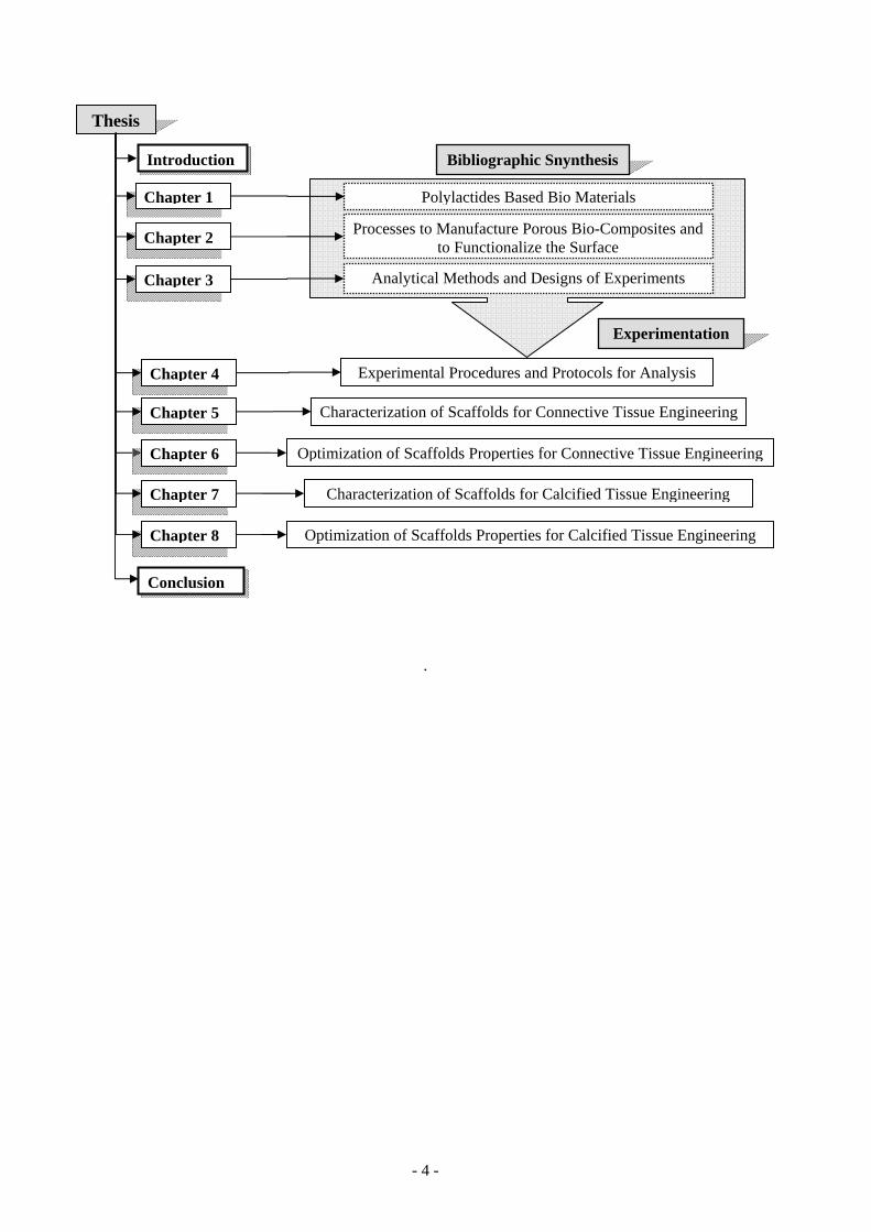
- 4 -
.
Thesis
Chapter 1
Chapter 2
Chapter 3
Chapter 4
Chapter 5
Chapter 6
Polylactides Based Bio Materials
Processes to Manufacture Porous Bio-Composites and to Functionalize the Surface
Analytical Methods and Designs of Experiments
Experimental Procedures and Protocols for Analysis
Characterization of Scaffolds for Connective Tissue Engineering
Optimization of Scaffolds Properties for Connective Tissue Engineering
Bibliographic Snynthesis
Experimentation
Chapter 7
Chapter 8
Characterization of Scaffolds for Calcified Tissue Engineering
Optimization of Scaffolds Properties for Calcified Tissue Engineering
Introduction
Conclusion
5
Chapter 1
Chapter 1
Polylactides Based Bio-Materials
In this chapter, we present a bibliographic synthesis divided in three parts. The first one deals with generalities on bio-composites, their uses in tissue engineering and bone regeneration applications. The second one concerns polyester based biomaterials, and in particular those used in this study polylactides such as polylactic acid and poly (lactide-co-glycolide acid). Finally, the third part deals with
adjuvant and fillers. We focus on hyaluronic acid, amorphous calcium phosphate and - calcium phosphate
which are the fillers retained for the study.
1 Introduction to Bio Composites
A bio-composite is a material formed by a matrix (resin) and a reinforcement of natural fibres or particles (usually derived from plants or cellulose). Their application has wide-range uses from environment-friendly biodegradable composites to biomedical composites for drug/gene delivery, tissue engineering applications and cosmetic orthodontics. They often mimic the structures of the living materials involved in the process in addition to the strengthening properties of the matrix that was used but still providing biocompatibility, e.g. in creating scaffolds in bone and cartilage tissue engineering. Such markets are significantly rising, mainly because of the increase in oil price, and recycling and environment
necessities. Bio-composites are characterised by the fact that:
the petrochemical resin is replaced by a vegetable or animal resin, and/or
the bolsters (fibreglass, carbon fibre or talc) are replaced by natural fibres (wood fibres, hemp, flax,
sisal, jute etc.).
In biomaterials, it is important that each constituent of the composite must be biocompatible and biodegradable. Moreover, the interface between constituents should not be degraded by the body
environment. Normally, bio-composite materials can be classified into three groups:
Particulate composites,
Fibrous composites,
Chapter 1. Polylactide Based Bio-Materials
- 6 -
Porous materials.
1.1 Bio-composites for 3D Model of Connective Tissues
1.1.1 Tissue Engineering and Concept of Scaffold
The scaffold for supporting 3D cell culture must meet a number of criteria to function appropriately and to promote tumour growth. These criteria include both mechanical parameters as well as parameters of biological performance. Biocompatibility of the scaffold is critical and must not damage cells and alter their functions or lead to significant scarring. To minimize undesirable effects, it is better to use inert scaffolds such as silk or chitin for example. Furthermore cells or matrices from different species can be used. For example, the use of a murine matrix together with human cells will allow studying the production and deposition of matrix proteins produced by tumour cells. Furthermore, differences in tensional forces may impact the phenotype of cancer cells. Thus, it is critical to minimize these differences in specific
experimental conditions.
1.1.2 Different Types of Scaffolds
Different types of three dimensional in vitro cancer models exist.
1.1.2.1 Cells Grown in Pellets or in Spheroids
Cells cultured as spheroids are formed by self-assembly. They mimic vascular tumours and micro-metastases. Tedious procedures required for formation, maintenance, and culture conditions are still holding back the industry from using a validated spheroid model more widely. Spheroid preparations on a chip using micro-fluid devices have been reported [Hsiao et al., 2009]. However, these methods suffer from problems with regard to spheroid formation, long-term culture, control of spheroid size and uniform distribution of
small numbers of co-culture cell types across all spheroids.
1.1.2.2 Cells Embedded into Hydrogels Derived from Natural or Synthetic Polymers
Naturally derived polymers (alginates, agarose or collagen) frequently demonstrate adequate biocompatibility, while synthetic polymers may be problematic. During gelling, ionic interference could occur with multivalent counter ions that exchange with other ionic molecules resulting in an uncontrolled deterioration of the hydrogel. Toxicity of cross-linking molecules must also be considered [Mooney and Silva, 2007]. Another approach to form hydrogel is the utilization of phase transition behaviour of certain polymers, which may help to overcome these problems [Castelló-Cros and Cukierman, 2009]. The interaction of cells with hydrogels significantly affects their adhesion as well as migration and differentiation. The adhesion is dependent on the interaction of specific cell surface receptors with ligands that may be integrated into the material. Inappropriate interactions in the hydrogel may cause non-adequate growth behaviour. Collagen that may be integrated in the gel has many of the biological properties of a natural environment. However, variations between collagen batches may be found. Its derivative, gelatine, easily forms gels by changes in the temperature of the solution. The chemical modification methods to
improve the mechanical properties of gelatine gels may also interfere with cell behaviour.
1.1.2.3 Cells Grown in a Biomaterial of Large–size on Different Polymers (PLGA,
Agarose)
Tumour cells cultured in porous PLGA (poly(lactide-co-glycolide)) scaffolds proliferate and form cohesive tumour cell aggregates in vitro. The final scaffold is about one cm in diameter and one mm in thickness. Cells in the scaffold must be cultured on an orbital shaker for up to 15 days. Comparison with standard 3D-Matrigel® culture show that tumour cells proliferate much more rapidly inside the scaffold and
Chapter 1. Polylactide Based Bio-Materials
- 7 -
that secretion of some specific growth factors is up-regulated. Other requirements are a good porosity and the need of bioreactors and gas exchanges during culture. Tumour cells may also be implanted in the scaffold subcutaneously in the back of mice. This method is limited because no up-scaling of this procedure is possible and no observation is possible during culture. These models seem to be restricted to research
laboratories.
1.1.2.4 Cells Grown in a Biomaterial at a Micrometer-Scale (Thickness ~200 µm)
This material has its limitation because cells may behave differently depending on the batch of reconstituted basement membrane extract (BME) called Matrigel®, they are grown on. Because BME is a natural product made from extracts of mouse sarcomas, it is difficult to get uniform, consistent preparations, even from the same manufacturer. The solution is to test and to stock validated batches of BME. There are several other methods such as matrix production by fibroblasts or mixture of tumour cells and matrix. For the former, alkaline treatment removes cells that leave behind complex substrates of fibronectin, collagen, and other proteins. Progression of the tumours deriving from these matrices laid down normal fibroblasts [Fischbach et al., 2007]. For the latter, a gel mixture is prepared by mixing an extracellular matrix (ECM) with tumour cells and Matrigel® (volume to volume 1:1) that allows the solution to polymerize. The
resulting 3D scaffold on which tumour cells are cultured is not the pure ECM, they would encounter in vivo.
Another alternative is to use commercial 3D matrices. These are, for example, reconstituted basement membrane extract such as Matrigel® (Sigma). Matrigel® is used to support growth and differentiation of cells and tissues. It recapitulates the morphology and visco-elasticity of the extracellular matrix and can be remodelled by cells. The drawbacks are that it is expensive and the composition is variable. Alternatively, interstitial matrix components such as collagen, fibrin, etc may be used. They are frequently employed to study migration and invasion. These matrix proteins can be remodelled by cells, and are often used in combination. However, their use may be problematic because glycosylation and solubility may vary by source and the properties between native and denatured proteins may differ. There are other
commercially available matrices such as (semi)-synthetic hydrogels proposed by BD (PuraMatrix peptide
hydrogel). It often polymerizes in combination with bioactive peptides. The drawbacks are that it shows some bioactivity with certain cells and it cannot be remodelled or degraded by cells. Other ready-to-use
systems are the algiMatrix3D® culture system (invitrogen) that comes as sponges in 96-well plates or
InsertTM-PCL (3D Biotek®), a biodegradable polycaprolactone scaffold. These systems are quite
expensive. Other authors Castelló-Cros and Cukierman [2009] have used 3D agarose colony formation and
GelCount technology with GelCount scan and image acquisition for high-resolution scanner allowing
the calculation of half maximal inhibitory concentration (IC50). This system provides quantitative data (log dose and time-dependent effects of drugs). However, no description of the gel (thickness) and of the quality of colonies formed is reported for this model (size of the colony, interactions between cells, and the
distribution of the cells across the colony).
1.2 Bio-Composites for Calcified Tissue Engineering
1.2.1 Composition of Scaffolds
The principal calcified tissue of vertebrates is bone. Other calcified tissues in vertebrates include calcified cartilage, which is present to some extent in most bones and the dental tissues - enamel, cementum, and dentin. Bone develops by the process of ossification, osteogenesis, as a specialized connective tissue. During ossification, osteoblasts secrete an amorphous material, gradually becoming densely fibrous - osteoid. Calcium phosphate crystals are deposited in the osteoid (i.e. mineralization), thereby becoming bone matrix. Osteoblasts become surrounded during the mineralization process, and the cells become osteocytes.
Chapter 1. Polylactide Based Bio-Materials
- 8 -
Osteoblast secretion does not become entirely fibrous. The secretion also forms an amorphous adhesion
between the fibres [Lee and Chuong, 2009].
Many studies can be found in the literature pursuing the aim to produce biomimetic artificial bone-like tissue involving hydoxyapatite (HAp) and collagen as fibre, gel or gelatine [Kim et al., 2005; Kikuchi et al., 2004; Tampieri et al., 2003a; Itoh et al., 2001]. Testing two methods of preparation of apatite/collagen composite materials (dispersion of HAp in collagen gel or direct nucleation of HAp into collagen fibres), Tampieri et al .[2003b] have shown that the bio-inspired method based on the direct nucleation of apatite leads to composites analogous to calcified tissue and exhibiting strong interactions
between HAp and collagen.
The replacement and healing of damaged hard tissues have always been a concern for human beings as shown by the examination of mummies. It is however known that calcium phosphates have been used for bone substitution and repair [Jarcho et al., 1979]. The first to be used were stoichiometric
hydroxyapatite and tricalcium phosphate (TCP) which are stable calcium phosphates at high temperature
and can be easily sintered into ceramics. They are still the major industrial calcium phosphates biomaterials.
TCP was shown to be bio-absorbable and replaced by bone whereas HAp constituted non-degradable
materials. TCP is mainly used as a bio-ceramic whereas HAp is also being processed for other biomaterials
uses such as the coating of metallic prostheses where it was found to considerably improve bone repair as an "osteo-conductive" material or composite ceramic/polymer materials showing strong mechanical analogies with bone tissues and excellent bone bonding abilities [De Groot et al., 1987]. Biphasic calcium phosphates, associating these two high-temperature calcium phosphates allow a controlled resorption rate and have been reported to offer superior biological properties [Daculsi et al., 2003; LeGeros, 2002]. They are progressively
replacing TCP ceramics in Europe. A new technological step was made with the development of calcium
phosphates cements [Brown and Chow, 1987]. These materials are able to set and harden in a living body and most can be injected. Despite their poor mechanical properties they offer a number of advantages and are increasingly used for several applications. More recently biomimetic coatings involving low temperature nano-crystalline calcium phosphates have been proposed, some have been claimed to exhibit osteo-inductive
properties [Habibovic et al., 2006].
1.2.2 Mechanical Properties of 3D Porous Scaffolds
The scaffold for tissue engineering should have a 3D porous structure with a porosity of no less than 70% and a pore size ranging from 50 to 900 μm [Salgado et al., n.d.]. High scaffold porosity facilitates oxygen, nutrient and metabolic product exchange. The literature results showed that with the optimization design, the porosity of the scaffolds was 82.0 ± 3.8%. It was composed of the designed interconnectivity macro-pores and micro-pores. The interconnectivity macro-pores in 3D scaffold would help develop the skeletal network and facilitate the internal mineralized bone formation [Cerroni et al., 2002]. The micro-pores less than 50 μm on the walls of the macro-pores would help in factors like fluid diffusion and cell attachment. Additionally, the scaffold for bone tissue engineering should also have high mechanical strength as close as possible to the strength of natural bone [Hutmacher, 2000]. In this study, the compressive strength and elastic modulus of the calcium phosphate/PLGA scaffolds were significantly higher than those of the pure PLGAs scaffolds. This result was consistent with some studies that improved the mechanical properties of biodegradable polymers by adding inorganic materials [Zhang and Zhang, 2001; Thomson et al., 1998]. However, co-grinding with calcium phosphate increased the mechanical properties and structural
quality but the porosity and pore diameter of the scaffolds was decreased.
Compressive modulus values of human trabecular bone range from 1 to 5000 MPa, with strength values ranging from 0.10 to 27.3 MPa reported by Langer and Tirrell [2004]; Porter et al. [2000]; Lang et
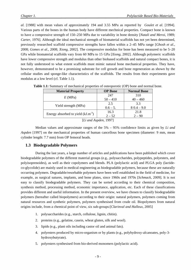
Chapter 1. Polylactide Based Bio-Materials
- 9 -
al. [1988] with mean values of approximately 194 and 3.55 MPa as reported by Goulet et al. [1994]. Various parts of the bones in the human body have different mechnical properties. Compact bone is known to have a compressive strength of 150–250 MPa due to variability in bone density [Natali and Meroi, 1989; Carter, 1976]. Although the ideal mechanical strength of biomaterial scaffolds has not yet been determined, previously researched scaffold compressive strengths have fallen within a 2–45 MPa range [Ghosh et al., 2008; Gomes et al., 2008; Xiong, 2002]. The compressive modulus for bone has been measured to be 5–20 GPa while biomaterial scaffolds vary from 60 MPa to 15 GPa [Xiong, 2002]. Although polymeric scaffolds have lower compressive strength and modulus than other biobased scaffolds and natural compact bones, it is not fully understood to what extent scaffolds must mimic natural bone mechanical properties. They have, however, demonstrated to be a promising substrate for cell growth and bone regeneration as shown by the cellular studies and sponge-like characteristics of the scaffolds. The results from their experiments gave
modulus at a low level (cf. Table 1.1).
Table 1.1: Summary of mechanical properties of osteoporotic (OP) bone and normal bone.
Material Property OP Bone Normal Bone
E (MPa) 247
50 – 410 310
40 – 460
Yield strength (MPa) 2.5
0.6 – 5. 3.3
8 0.4 – 9.0
Energy absorbed to yield (kJ.m-3) 16.3
2 – 52 21.8
2 – 90 [Li and Aspden, 1997]
Median values and approximate ranges of the 5% – 95% confidence limits as given by Li and Aspden [1997] on the mechanical properties of human cancellous bone specimen (diameter: 9 mm, mean
cylinder length: 7.7 mm) from OP femoral heads.
1.3 Biodegradable Polymers
During the last years, a large number of articles and publications have been published which cover biodegradable polymers of the different material groups (e.g., polysaccharides, polypeptides, polyesters, and polyisoprenoides), as well as their copolymers and blends. PLA (polylactic acid) and PLGA poly (lactide-co-glycolide) are mainly used in medical engineering as biodegradable polymers, because these are naturally occurring polymers. Degradable/resorbable polymers have been well established in the field of medicine, for example, as surgical sutures, implants, and bone plates, since 1960s and 1970s [Schmack, 2009]. It is not easy to classify biodegradable polymers. They can be sorted according to their chemical composition, synthesis method, processing method, economic importance, application, etc. Each of these classifications provides different and useful information. In the present overview, we have chosen to classify biodegradable polymers (hereafter called biopolymers) according to their origin: natural polymers, polymers coming from natural resources and synthetic polymers, polymers synthesised from crude oil. Biopolymers from natural
origins include, from a chemical point of view, six sub-groups:[Clarinval and Halleux, 2005]
1. polysaccharides (e.g., starch, cellulose, lignin, chitin).
2. proteins (e.g., gelatine, casein, wheat gluten, silk and wool).
3. lipids (e.g., plant oils including castor oil and animal fats).
4. polyesters produced by micro-organism or by plants (e.g., polyhydroxy-alcanoates, poly-3-hydroxybutyrate).
5. polyesters synthesised from bio-derived monomers (polylactic acid).
Chapter 1. Polylactide Based Bio-Materials
- 10 -
6. a final group of miscellaneous polymers (natural rubbers, composites).
1.3.1 What is Biodegradable?
Biodegradation is degradation caused by biological activity, particularly by enzyme action leading to significant changes in the material's chemical structure, or by UV radiations which are natural and participate also to biodegradation. In essence, biodegradable plastics should breakdown cleanly, in a defined time period, to simple molecules found in the environment such as carbon dioxide and water. The American Society of Testing and Materials (ASTM) defines 'biodegradability' as: "capable of undergoing decomposition into carbon dioxide, methane, water, inorganic compounds, or biomass in which the predominant mechanism is the enzymatic action of microorganisms, that can be measured by standardized
tests in a specified period of time, reflecting available disposal conditions."
During this process of biodegradation, the large molecules of the substance are transformed into smaller compounds by enzymes and acids that are naturally produced by microorganisms. Once the molecules are reduced to a suitable size, the substances can be absorbed through the organism cell walls where they are metabolized for energy. Most naturally occurring materials such as yard waste, food scraps,
etc., contain these large molecules and biodegrade in this way.
1.3.1.1 Aerobic Biodegradation
Aerobic biodegradation is the breakdown of an organic substance by microorganisms in the presence of oxygen. Almost all organic materials can be metabolized in an oxidative environment by aerobic organisms. The organism has secreted enzymes that breakdown substances into smaller organic molecules which are then absorbed into the cells of the microbes and used for cellular respiration. During the respiration process, the organic molecules absorbed into the cells are broken down in steps, where a molecule known as adenosine-5-triphosphate (ATP) is used to store and transport energy for cells, for life processes such as motility and cell division. In biochemistry, this chemical reaction sequence is known as Electron Chain Transfer. In the case of aerobic metabolism, oxygen is used at the end of the chain as the final electron acceptor, producing the main by products of carbon dioxide and water. The chemistry of the key degradation process is represented by Equation 1.1, where CPolymer represents either a polymer or a
fragment from any of the degradation processes defined earlier [Bastioli, 2005]:
CPolymer + O2 CO2 + H2O + CResidue + CBiomass (1.1)
Composting is a well known and common use of aerobic biodegradation, during which the volume of organic material is typically reduced by about 50%, where the remaining, slow-decaying humus material left over can be used as a rich planting medium. The ASTM defines a compostable plastic material as being: “capable of biological decomposition in a compost site as part of an available program, such that the plastic is not visually distinguishable and breaks down to carbon dioxide, water inorganic compounds and biomass (humus) at a rate consistent with known compostable materials”. The bioactivity in active compost will generate heat that further enhances the rate of microbial growth and metabolism. However, for the purpose of the ASTM definition, the available program is an industrial compost facility where heat and moisture are artificially added to the mass to maximize the degradation rate. As we will see, this artificial
environment becomes critical for degradation of some biodegradable plastic materials.
1.3.1.2 Anaerobic Biodegradation
Anaerobic biodegradation occurs in the absence of oxygen where anaerobic microbes are dominant. In the absence of oxygen, the organism must use some other atoms as the final electron acceptor. Hydrogen, methane, nitrogen and sulphur are common along with oxidizing minerals. Thus, the effluent
Chapter 1. Polylactide Based Bio-Materials
- 11 -
from anaerobic digestion is biogas, consisting of mostly methane and carbon dioxide, with trace gasses such as ammonia and hydrogen sulphide. Often, the complete digestion will require several different types of bacteria where one type partially processes the waste to a point where another bacterium strain takes over. Most biodegradation of solid waste in landfill occurs under anaerobic conditions by design because it is typically much slower than aerobic degradation. In the absence of oxygen, the reaction of degradation is
given by equation 1.2:
CPolymer → CO2 + CH4 + H2O + + CResidue + CBiomass (1.2)
Complete biodegradation occurs when no residue remains, and complete mineralisation is established when the original substrate (CPolymer in this example) is completely converted into gaseous products and salts. However, mineralisation is a very slow process under natural conditions because some of the polymer undergoing biodegradation will initially be turned into biomass [Bastioli, 2005]. Most biodegradable substances come from plant and animal matter, or from artificial materials that are very similar in molecular structure to these naturally occurring substances. As the naturally occurring substances evolved, micro-organisms also evolved to use the substances as a food source, carbon in particular, used as a building block for life-sustaining compounds. Simple sugars are readily absorbed into the cell to be metabolized. However, larger and more complex molecules such as starches, proteins and cellulose, require enzymes and acids to reduce their size enough to be absorbed. Living organisms have developed the ability to secrete specific digestive compounds so as to best utilize the available food supply. For example, the enzyme amylase, found in human saliva, is used to breakdown long-chain starch molecules into smaller
simple sugars.
1.3.2 Biodegradable Polymer Materials
Currently available degradable polymer materials can be broken down into two main groups:
Polyester polymers,
Synergistic and hybrid polymers.
1.3.2.1 Biodegradable Polyesters
Biodegradable polyesters which do not contain six-carbon rings are known as aliphatic polyesters. They will typically react with moisture at elevated temperatures to breakdown the long polymer chains. This process, called chemical hydrolysis, reduces the higher molecular weight polymer to much smaller hydrocarbon compounds. The resulting molecules can then be absorbed by microorganisms and metabolized for energy. Since it is a chemical reaction, the hydrolysis occurs at a much higher rate than one would expect
for a purely biological process, and as a result, relatively quick degradation is observed.
Aliphatic polyesters have attracted interest as biodegradable plastic materials; however they typically have poor physical and mechanical properties like strength, flexibility, heat resistance, etc. [Chen et al., 2008]. Some common biodegradable polyester polymers in commercial use include poly(caprolactone), poly(glycolic acid) and poly(butylene succinate) (cf. chemical formula reported on Figure 1.1). Although expensive to make, these biodegradable polymers are ideal for use in specialized, high margin applications such as medical devices (e.g. dissolving, drug delivery systems, tissue engineering
scaffolds and bone repair etc.) [Ikada and Tsuji, 1999].
Another well known aliphatic polyester is poly(lactic acid). PLA is a synthetic polymer made from fermented sugars extracted primarily from food crops such as corn, beets or sugarcane. The resulting lactic acid monomer is chemically processed and then polymerized, in the presence of a metal catalyst, to form the high molecular weight plastic material. Like petroleum-based biodegradable polyesters, PLA has
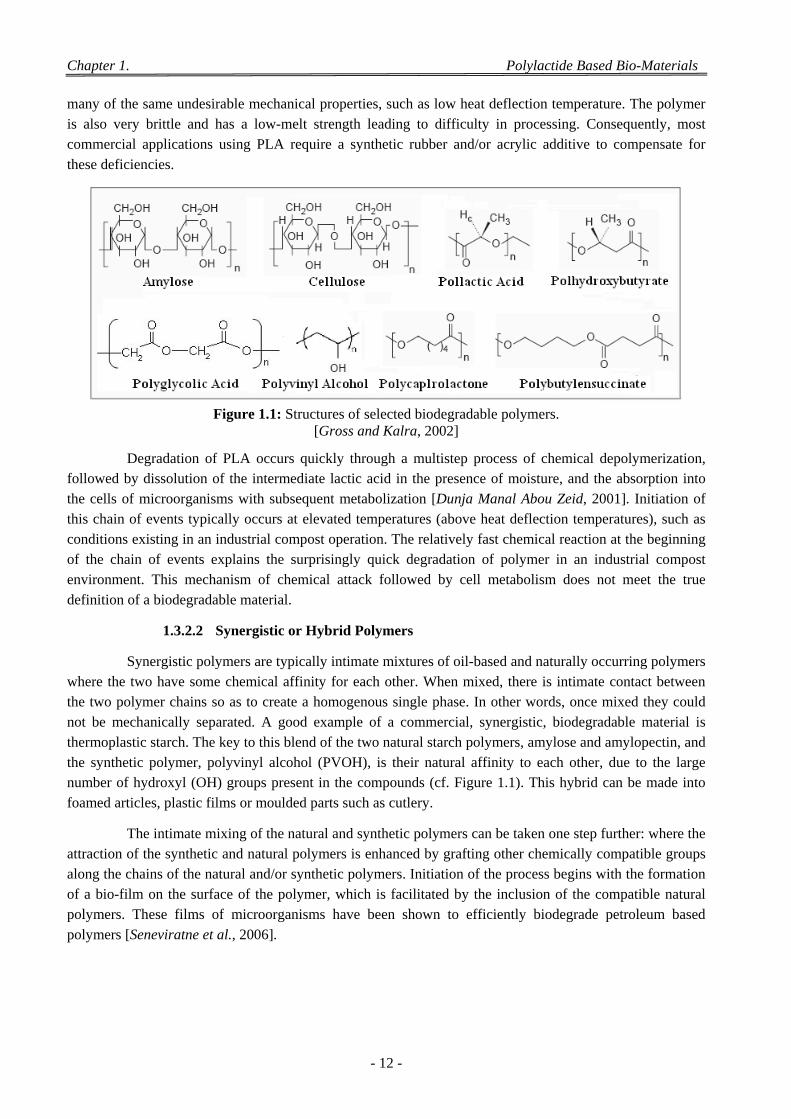
Chapter 1. Polylactide Based Bio-Materials
- 12 -
many of the same undesirable mechanical properties, such as low heat deflection temperature. The polymer is also very brittle and has a low-melt strength leading to difficulty in processing. Consequently, most commercial applications using PLA require a synthetic rubber and/or acrylic additive to compensate for
these deficiencies.
Figure 1.1: Structures of selected biodegradable polymers.
[Gross and Kalra, 2002]
Degradation of PLA occurs quickly through a multistep process of chemical depolymerization, followed by dissolution of the intermediate lactic acid in the presence of moisture, and the absorption into the cells of microorganisms with subsequent metabolization [Dunja Manal Abou Zeid, 2001]. Initiation of this chain of events typically occurs at elevated temperatures (above heat deflection temperatures), such as conditions existing in an industrial compost operation. The relatively fast chemical reaction at the beginning of the chain of events explains the surprisingly quick degradation of polymer in an industrial compost environment. This mechanism of chemical attack followed by cell metabolism does not meet the true
definition of a biodegradable material.
1.3.2.2 Synergistic or Hybrid Polymers
Synergistic polymers are typically intimate mixtures of oil-based and naturally occurring polymers where the two have some chemical affinity for each other. When mixed, there is intimate contact between the two polymer chains so as to create a homogenous single phase. In other words, once mixed they could not be mechanically separated. A good example of a commercial, synergistic, biodegradable material is thermoplastic starch. The key to this blend of the two natural starch polymers, amylose and amylopectin, and the synthetic polymer, polyvinyl alcohol (PVOH), is their natural affinity to each other, due to the large number of hydroxyl (OH) groups present in the compounds (cf. Figure 1.1). This hybrid can be made into
foamed articles, plastic films or moulded parts such as cutlery.
The intimate mixing of the natural and synthetic polymers can be taken one step further: where the attraction of the synthetic and natural polymers is enhanced by grafting other chemically compatible groups along the chains of the natural and/or synthetic polymers. Initiation of the process begins with the formation of a bio-film on the surface of the polymer, which is facilitated by the inclusion of the compatible natural polymers. These films of microorganisms have been shown to efficiently biodegrade petroleum based
polymers [Seneviratne et al., 2006].
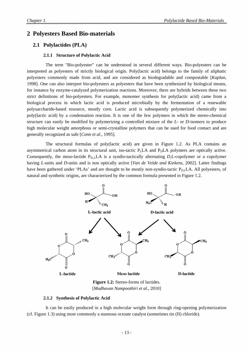
Chapter 1. Polylactide Based Bio-Materials
- 13 -
2 Polyesters Based Bio-materials
2.1 Polylactides (PLA)
2.1.1 Structure of Polylactic Acid
The term "Bio-polyester" can be understood in several different ways. Bio-polyesters can be interpreted as polyesters of strictly biological origin. Poly(lactic acid) belongs to the family of aliphatic polyesters commonly made from acid, and are considered as biodegradable and compostable [Kaplan, 1998]. One can also interpret bio-polyesters as polyesters that have been synthesized by biological means, for instance by enzyme-catalyzed polymerization reactions. Moreover, there are hybrids between these two strict definitions of bio-polyesters. For example, monomer synthesis for poly(lactic acid) came from a biological process in which lactic acid is produced microbially by the fermentation of a renewable polysaccharide-based resource, mostly corn. Lactic acid is subsequently polymerized chemically into poly(lactic acid) by a condensation reaction. It is one of the few polymers in which the stereo-chemical structure can easily be modified by polymerizing a controlled mixture of the L- or D-isomers to produce high molecular weight amorphous or semi-crystalline polymers that can be used for food contact and are
generally recognized as safe [Conn et al., 1995].
The structural formulas of poly(lactic acid) are given in Figure 1.2. As PLA contains an asymmetrical carbon atom in its structural unit, iso-tactic PLLA and PDLA polymers are optically active. Consequently, the meso-lactide PD,,LLA is a syndio-tactically alternating D,L-copolymer or a copolymer having L-units and D-units and is non optically active [Van de Velde and Kiekens, 2002]. Latter findings have been gathered under ‘PLAs’ and are thought to be mostly non-syndio-tactic PD,LLA. All polyesters, of
natural and synthetic origins, are characterized by the common formula presented in Figure 1.2.
Figure 1.2: Stereo-forms of lactides. [Madhavan Nampoothiri et al., 2010]
2.1.2 Synthesis of Polylactic Acid
It can be easily produced in a high molecular weight form through ring-opening polymerization
(cf. Figure 1.3) using most commonly a stannous octoate catalyst (sometimes tin (II) chloride).
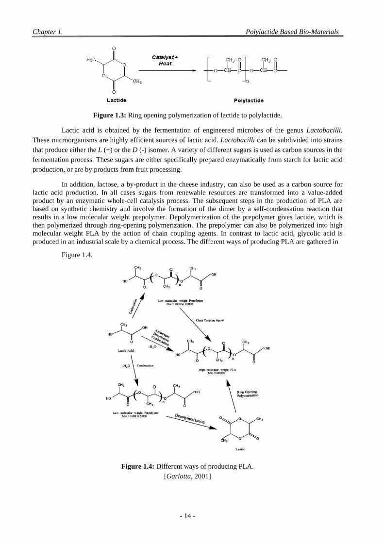
Chapter 1. Polylactide Based Bio-Materials
- 14 -
Figure 1.3: Ring opening polymerization of lactide to polylactide.
Lactic acid is obtained by the fermentation of engineered microbes of the genus Lactobacilli. These microorganisms are highly efficient sources of lactic acid. Lactobacilli can be subdivided into strains that produce either the L (+) or the D (-) isomer. A variety of different sugars is used as carbon sources in the fermentation process. These sugars are either specifically prepared enzymatically from starch for lactic acid
production, or are by products from fruit processing.
In addition, lactose, a by-product in the cheese industry, can also be used as a carbon source for lactic acid production. In all cases sugars from renewable resources are transformed into a value-added product by an enzymatic whole-cell catalysis process. The subsequent steps in the production of PLA are based on synthetic chemistry and involve the formation of the dimer by a self-condensation reaction that results in a low molecular weight prepolymer. Depolymerization of the prepolymer gives lactide, which is then polymerized through ring-opening polymerization. The prepolymer can also be polymerized into high molecular weight PLA by the action of chain coupling agents. In contrast to lactic acid, glycolic acid is produced in an industrial scale by a chemical process. The different ways of producing PLA are gathered in
Figure 1.4.
Figure 1.4: Different ways of producing PLA. [Garlotta, 2001]
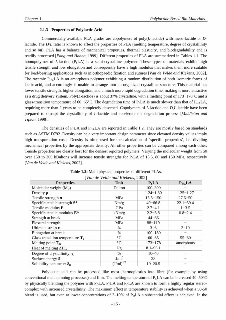
Chapter 1. Polylactide Based Bio-Materials
- 15 -
2.1.3 Properties of Polylactic Acid
Commercially available PLA grades are copolymers of poly(L-lactide) with meso-lactide or D-lactide. The D/L ratio is known to affect the properties of PLA (melting temperature, degree of crystallinity and so on). PLA has a balance of mechanical properties, thermal plasticity, and biodegradability and is readily processed [Fang and Hanna, 1999]. Different properties of PLA are summarized in Tables 1.1. The homopolymer of L-lactide (PLLA) is a semi-crystalline polymer. These types of materials exhibit high tensile strength and low elongation and consequently have a high modulus that makes them more suitable for load-bearing applications such as in orthopaedic fixation and sutures [Van de Velde and Kiekens, 2002]. The racemic PD,LLA is an amorphous polymer exhibiting a random distribution of both isomeric forms of lactic acid, and accordingly is unable to arrange into an organized crystalline structure. This material has lower tensile strength, higher elongation, and a much more rapid degradation time, making it more attractive as a drug delivery system. Poly(L-lactide) is about 37% crystalline, with a melting point of 173−178°C and a glass-transition temperature of 60−65°C. The degradation time of PLLA is much slower than that of PD,LLA, requiring more than 2 years to be completely absorbed. Copolymers of L-lactide and D,L-lactide have been prepared to disrupt the crystallinity of L-lactide and accelerate the degradation process [Middleton and
Tipton, 1998].
The densities of PLLA and PD,LLA are reported in Table 1.2. They are mostly based on standards such as ASTM D792. Density can be a very important design parameter since elevated density values imply high transportation costs. Density is often used for the calculation of ‘specific properties’, i.e. dividing mechanical properties by the appropriate density. All other properties can be compared among each other. Tensile properties are clearly best for the densest reported polymers. Varying the molecular weight from 50 over 150 to 200 kDaltons will increase tensile strengths for PLLA of 15.5, 80 and 150 MPa, respectively
[Van de Velde and Kiekens, 2002].
Table 1.2: Main physical properties of different PLAs.
[Van de Velde and Kiekens, 2002] Properties Unit PLLA PD,LLA
Molecular weight (Mw) Dalton 100–300 − Density ρ - 1.24−1.30 1.25−1.27 Tensile strength σ MPa 15.5−150 27.6−50 Specific tensile strength S* Nm/g 40−66.8 22.1−39.4 Tensile modulus E GPa 2.7−4.1 1−3.5 Specific tensile modulus E* kNm/g 2.2−3.8 0.8−2.4 Strength at break MPa 44−66 − Flexural strength MPa 88−119 − Ultimate strain ε % 3−6 2−10 Elongation at break % 100–180 − Glass transition temperature Tg °C 60−65 55−60 Melting point Tm °C 173−178 amorphous Heat of melting Hm J/g 8.1–93.1 − Degree of crystallinity, % 10–40 − Surface energy J/m2 38 − Solubility parameter δH (J/ml)1/2 19–20.5 −
Polylactic acid can be processed like most thermoplastics into fibre (for example by using conventional melt spinning processes) and film. The melting temperature of PLLA can be increased 40–50°C by physically blending the polymer with PDLA. PLLA and PDLA are known to form a highly regular stereo-complex with increased crystallinity. The maximum effect in temperature stability is achieved when a 50-50 blend is used, but even at lower concentrations of 3–10% of PDLA a substantial effect is achieved. In the
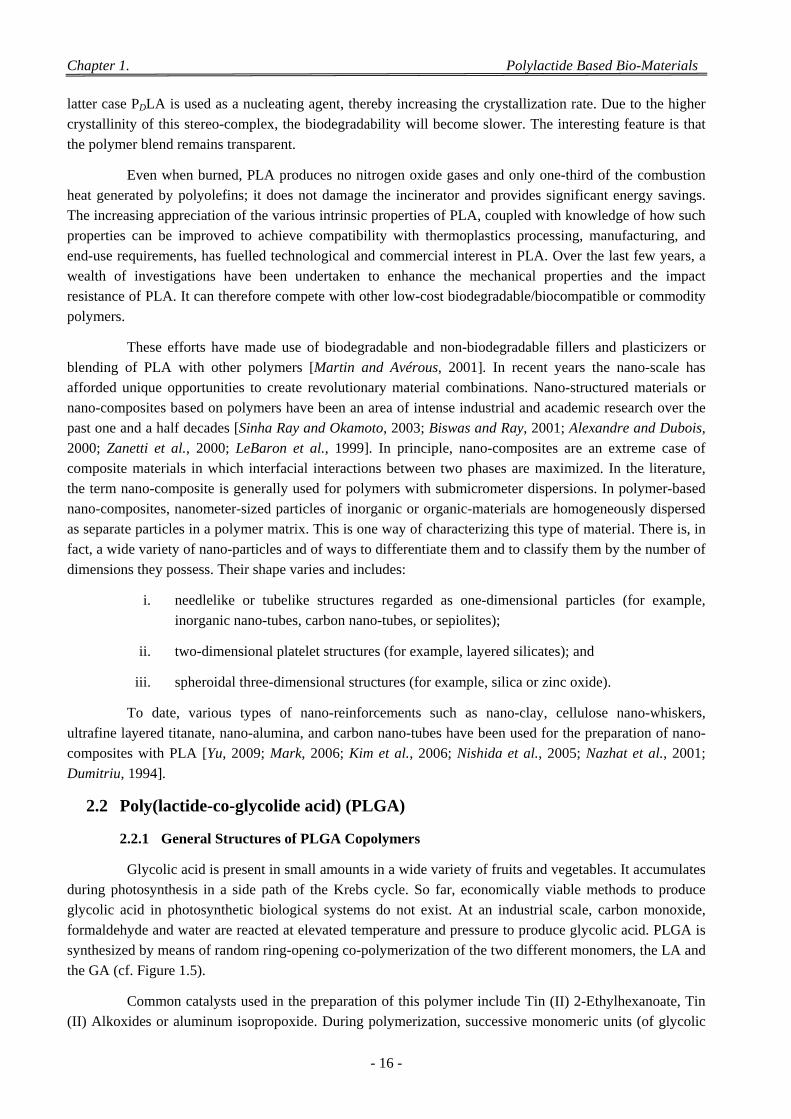
Chapter 1. Polylactide Based Bio-Materials
- 16 -
latter case PDLA is used as a nucleating agent, thereby increasing the crystallization rate. Due to the higher crystallinity of this stereo-complex, the biodegradability will become slower. The interesting feature is that
the polymer blend remains transparent.
Even when burned, PLA produces no nitrogen oxide gases and only one-third of the combustion heat generated by polyolefins; it does not damage the incinerator and provides significant energy savings. The increasing appreciation of the various intrinsic properties of PLA, coupled with knowledge of how such properties can be improved to achieve compatibility with thermoplastics processing, manufacturing, and end-use requirements, has fuelled technological and commercial interest in PLA. Over the last few years, a wealth of investigations have been undertaken to enhance the mechanical properties and the impact resistance of PLA. It can therefore compete with other low-cost biodegradable/biocompatible or commodity
polymers.
These efforts have made use of biodegradable and non-biodegradable fillers and plasticizers or blending of PLA with other polymers [Martin and Avérous, 2001]. In recent years the nano-scale has afforded unique opportunities to create revolutionary material combinations. Nano-structured materials or nano-composites based on polymers have been an area of intense industrial and academic research over the past one and a half decades [Sinha Ray and Okamoto, 2003; Biswas and Ray, 2001; Alexandre and Dubois, 2000; Zanetti et al., 2000; LeBaron et al., 1999]. In principle, nano-composites are an extreme case of composite materials in which interfacial interactions between two phases are maximized. In the literature, the term nano-composite is generally used for polymers with submicrometer dispersions. In polymer-based nano-composites, nanometer-sized particles of inorganic or organic-materials are homogeneously dispersed as separate particles in a polymer matrix. This is one way of characterizing this type of material. There is, in fact, a wide variety of nano-particles and of ways to differentiate them and to classify them by the number of
dimensions they possess. Their shape varies and includes:
i. needlelike or tubelike structures regarded as one-dimensional particles (for example, inorganic nano-tubes, carbon nano-tubes, or sepiolites);
ii. two-dimensional platelet structures (for example, layered silicates); and
iii. spheroidal three-dimensional structures (for example, silica or zinc oxide).
To date, various types of nano-reinforcements such as nano-clay, cellulose nano-whiskers, ultrafine layered titanate, nano-alumina, and carbon nano-tubes have been used for the preparation of nano-composites with PLA [Yu, 2009; Mark, 2006; Kim et al., 2006; Nishida et al., 2005; Nazhat et al., 2001;
Dumitriu, 1994].
2.2 Poly(lactide-co-glycolide acid) (PLGA)
2.2.1 General Structures of PLGA Copolymers
Glycolic acid is present in small amounts in a wide variety of fruits and vegetables. It accumulates during photosynthesis in a side path of the Krebs cycle. So far, economically viable methods to produce glycolic acid in photosynthetic biological systems do not exist. At an industrial scale, carbon monoxide, formaldehyde and water are reacted at elevated temperature and pressure to produce glycolic acid. PLGA is synthesized by means of random ring-opening co-polymerization of the two different monomers, the LA and
the GA (cf. Figure 1.5).
Common catalysts used in the preparation of this polymer include Tin (II) 2-Ethylhexanoate, Tin (II) Alkoxides or aluminum isopropoxide. During polymerization, successive monomeric units (of glycolic
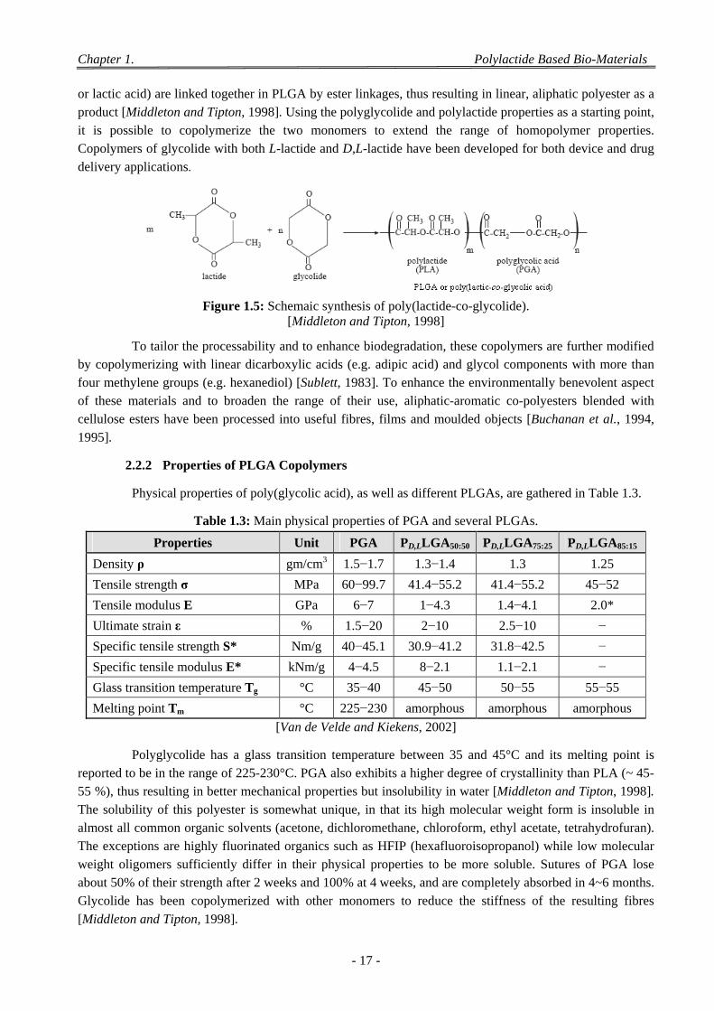
Chapter 1. Polylactide Based Bio-Materials
- 17 -
or lactic acid) are linked together in PLGA by ester linkages, thus resulting in linear, aliphatic polyester as a product [Middleton and Tipton, 1998]. Using the polyglycolide and polylactide properties as a starting point, it is possible to copolymerize the two monomers to extend the range of homopolymer properties. Copolymers of glycolide with both L-lactide and D,L-lactide have been developed for both device and drug
delivery applications.
Figure 1.5: Schemaic synthesis of poly(lactide-co-glycolide).
[Middleton and Tipton, 1998]
To tailor the processability and to enhance biodegradation, these copolymers are further modified by copolymerizing with linear dicarboxylic acids (e.g. adipic acid) and glycol components with more than four methylene groups (e.g. hexanediol) [Sublett, 1983]. To enhance the environmentally benevolent aspect of these materials and to broaden the range of their use, aliphatic-aromatic co-polyesters blended with cellulose esters have been processed into useful fibres, films and moulded objects [Buchanan et al., 1994,
1995].
2.2.2 Properties of PLGA Copolymers
Physical properties of poly(glycolic acid), as well as different PLGAs, are gathered in Table 1.3.
Table 1.3: Main physical properties of PGA and several PLGAs.
Properties Unit PGA PD,LLGA50:50 PD,LLGA75:25 PD,LLGA85:15
Density ρ gm/cm3 1.5−1.7 1.3−1.4 1.3 1.25
Tensile strength σ MPa 60−99.7 41.4−55.2 41.4−55.2 45−52
Tensile modulus E GPa 6−7 1−4.3 1.4−4.1 2.0*
Ultimate strain ε % 1.5−20 2−10 2.5−10 −
Specific tensile strength S* Nm/g 40−45.1 30.9−41.2 31.8−42.5 −
Specific tensile modulus E* kNm/g 4−4.5 8−2.1 1.1−2.1 −
Glass transition temperature Tg °C 35−40 45−50 50−55 55−55
Melting point Tm °C 225−230 amorphous amorphous amorphous
[Van de Velde and Kiekens, 2002]
Polyglycolide has a glass transition temperature between 35 and 45°C and its melting point is reported to be in the range of 225-230°C. PGA also exhibits a higher degree of crystallinity than PLA (~ 45-55 %), thus resulting in better mechanical properties but insolubility in water [Middleton and Tipton, 1998]. The solubility of this polyester is somewhat unique, in that its high molecular weight form is insoluble in almost all common organic solvents (acetone, dichloromethane, chloroform, ethyl acetate, tetrahydrofuran). The exceptions are highly fluorinated organics such as HFIP (hexafluoroisopropanol) while low molecular weight oligomers sufficiently differ in their physical properties to be more soluble. Sutures of PGA lose about 50% of their strength after 2 weeks and 100% at 4 weeks, and are completely absorbed in 4~6 months. Glycolide has been copolymerized with other monomers to reduce the stiffness of the resulting fibres
[Middleton and Tipton, 1998].
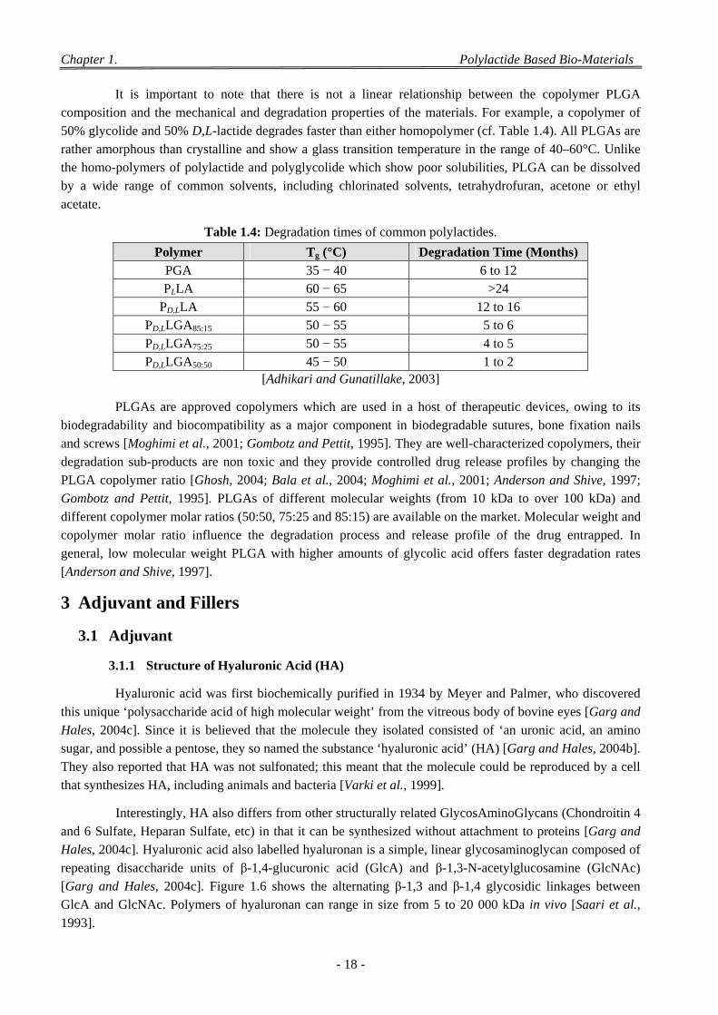
Chapter 1. Polylactide Based Bio-Materials
- 18 -
It is important to note that there is not a linear relationship between the copolymer PLGA composition and the mechanical and degradation properties of the materials. For example, a copolymer of 50% glycolide and 50% D,L-lactide degrades faster than either homopolymer (cf. Table 1.4). All PLGAs are rather amorphous than crystalline and show a glass transition temperature in the range of 40–60°C. Unlike the homo-polymers of polylactide and polyglycolide which show poor solubilities, PLGA can be dissolved by a wide range of common solvents, including chlorinated solvents, tetrahydrofuran, acetone or ethyl
acetate.
Table 1.4: Degradation times of common polylactides.
Polymer Tg (°C) Degradation Time (Months) PGA 35 − 40 6 to 12 PLLA 60 − 65 >24
PD,LLA 55 − 60 12 to 16 PD,LLGA85:15 50 − 55 5 to 6 PD,LLGA75:25 50 − 55 4 to 5 PD,LLGA50:50 45 − 50 1 to 2
[Adhikari and Gunatillake, 2003]
PLGAs are approved copolymers which are used in a host of therapeutic devices, owing to its biodegradability and biocompatibility as a major component in biodegradable sutures, bone fixation nails and screws [Moghimi et al., 2001; Gombotz and Pettit, 1995]. They are well-characterized copolymers, their degradation sub-products are non toxic and they provide controlled drug release profiles by changing the PLGA copolymer ratio [Ghosh, 2004; Bala et al., 2004; Moghimi et al., 2001; Anderson and Shive, 1997; Gombotz and Pettit, 1995]. PLGAs of different molecular weights (from 10 kDa to over 100 kDa) and different copolymer molar ratios (50:50, 75:25 and 85:15) are available on the market. Molecular weight and copolymer molar ratio influence the degradation process and release profile of the drug entrapped. In general, low molecular weight PLGA with higher amounts of glycolic acid offers faster degradation rates
[Anderson and Shive, 1997].
3 Adjuvant and Fillers
3.1 Adjuvant
3.1.1 Structure of Hyaluronic Acid (HA)
Hyaluronic acid was first biochemically purified in 1934 by Meyer and Palmer, who discovered this unique ‘polysaccharide acid of high molecular weight’ from the vitreous body of bovine eyes [Garg and Hales, 2004c]. Since it is believed that the molecule they isolated consisted of ‘an uronic acid, an amino sugar, and possible a pentose, they so named the substance ‘hyaluronic acid’ (HA) [Garg and Hales, 2004b]. They also reported that HA was not sulfonated; this meant that the molecule could be reproduced by a cell
that synthesizes HA, including animals and bacteria [Varki et al., 1999].
Interestingly, HA also differs from other structurally related GlycosAminoGlycans (Chondroitin 4 and 6 Sulfate, Heparan Sulfate, etc) in that it can be synthesized without attachment to proteins [Garg and Hales, 2004c]. Hyaluronic acid also labelled hyaluronan is a simple, linear glycosaminoglycan composed of repeating disaccharide units of β-1,4-glucuronic acid (GlcA) and β-1,3-N-acetylglucosamine (GlcNAc) [Garg and Hales, 2004c]. Figure 1.6 shows the alternating β-1,3 and β-1,4 glycosidic linkages between GlcA and GlcNAc. Polymers of hyaluronan can range in size from 5 to 20 000 kDa in vivo [Saari et al.,
1993].
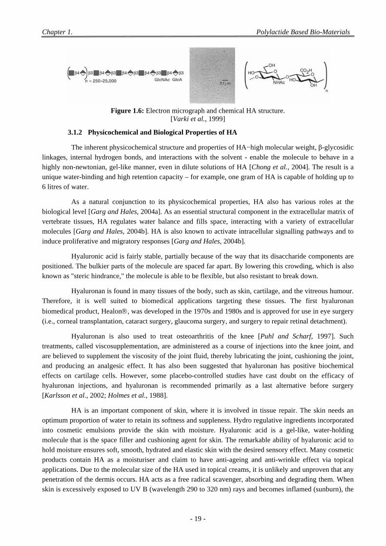
Chapter 1. Polylactide Based Bio-Materials
- 19 -
Figure 1.6: Electron micrograph and chemical HA structure.
[Varki et al., 1999]
3.1.2 Physicochemical and Biological Properties of HA
The inherent physicochemical structure and properties of HA−high molecular weight, β-glycosidic linkages, internal hydrogen bonds, and interactions with the solvent - enable the molecule to behave in a highly non-newtonian, gel-like manner, even in dilute solutions of HA [Chong et al., 2004]. The result is a unique water-binding and high retention capacity – for example, one gram of HA is capable of holding up to
6 litres of water.
As a natural conjunction to its physicochemical properties, HA also has various roles at the biological level [Garg and Hales, 2004a]. As an essential structural component in the extracellular matrix of vertebrate tissues, HA regulates water balance and fills space, interacting with a variety of extracellular molecules [Garg and Hales, 2004b]. HA is also known to activate intracellular signalling pathways and to
induce proliferative and migratory responses [Garg and Hales, 2004b].
Hyaluronic acid is fairly stable, partially because of the way that its disaccharide components are positioned. The bulkier parts of the molecule are spaced far apart. By lowering this crowding, which is also
known as "steric hindrance," the molecule is able to be flexible, but also resistant to break down.
Hyaluronan is found in many tissues of the body, such as skin, cartilage, and the vitreous humour. Therefore, it is well suited to biomedical applications targeting these tissues. The first hyaluronan
biomedical product, Healon, was developed in the 1970s and 1980s and is approved for use in eye surgery
(i.e., corneal transplantation, cataract surgery, glaucoma surgery, and surgery to repair retinal detachment).
Hyaluronan is also used to treat osteoarthritis of the knee [Puhl and Scharf, 1997]. Such treatments, called viscosupplementation, are administered as a course of injections into the knee joint, and are believed to supplement the viscosity of the joint fluid, thereby lubricating the joint, cushioning the joint, and producing an analgesic effect. It has also been suggested that hyaluronan has positive biochemical effects on cartilage cells. However, some placebo-controlled studies have cast doubt on the efficacy of hyaluronan injections, and hyaluronan is recommended primarily as a last alternative before surgery
[Karlsson et al., 2002; Holmes et al., 1988].
HA is an important component of skin, where it is involved in tissue repair. The skin needs an optimum proportion of water to retain its softness and suppleness. Hydro regulative ingredients incorporated into cosmetic emulsions provide the skin with moisture. Hyaluronic acid is a gel-like, water-holding molecule that is the space filler and cushioning agent for skin. The remarkable ability of hyaluronic acid to hold moisture ensures soft, smooth, hydrated and elastic skin with the desired sensory effect. Many cosmetic products contain HA as a moisturiser and claim to have anti-ageing and anti-wrinkle effect via topical applications. Due to the molecular size of the HA used in topical creams, it is unlikely and unproven that any penetration of the dermis occurs. HA acts as a free radical scavenger, absorbing and degrading them. When skin is excessively exposed to UV B (wavelength 290 to 320 nm) rays and becomes inflamed (sunburn), the
Chapter 1. Polylactide Based Bio-Materials
- 20 -
cells in the dermis stop producing as much HA and increase the rate of its degradation. HA degradation
products also accumulate in the skin after UV exposure [Averbeck et al., 2006].
Due to its high biocompatibility and its natural presence in the extracellular matrix of tissues, HA is gaining popularity as a biomaterial scaffold in tissue engineering research. In some cancers, HA levels correlate well with malignancy and poor prognosis. HA is thus often used as a tumor marker for prostate and
breast cancer. It may also be used to monitor the progression of the disease.
3.2 Calcium Phosphates and Tricalcium Phosphates
Seventy percent of bone is made up of hydroxyapatite [Ca10(PO4)6(OH)2], tooth enamel is also largely calcium phosphate. Like other apatites, it has a calcium and phosphate component in a ratio of 1.67 (Ca/P ratio) but is associated with a hydroxyl group. There are several other non-apatitic calcium phosphates that are distinguished from one another by their molecular formulae, Ca/P ratios that differ from 1.67, crystal
structures and solubilities, which have higher dissolution rates than stoichiometric hydroxyapatite.
3.2.1 Structures of Calcium Phosphate
Calcium phosphate Ca3(PO4)2 is the name given to a family of minerals containing calcium ions (Ca2+) together with orthophosphates (PO4
3-). Tricalcium phosphates (TCP) are among the most commonly-used calcium phosphates compounds in implant materials. They are found in ceramic bone substitutes, metallic prosthesis coatings, cements and composite materials. From a strict chemical point of view, ‘tricalcium phosphate’ refers to a composition, even though, in the minds of many users, this term is used to describe a structure, generally that of β tricalcium phosphate (βTCP). Tricalcium phosphates exist in four
different forms:
ATCP will hereby designate amorphous tricalcium phosphate;
Ap TCP: apatitic tricalcium phosphate: Ca9(HPO4)(PO4)5(OH);
TCP: the most widely used member of the TCP family having a crystalline structure: -Ca3(PO4)2;
TCP: the metastable high-temperature crystalline structure: α-Ca3(PO4)2.
Amorphous tricalcium phosphate (ATCP) and apatitic tricalcium phosphate (Ap TCP) are low
temperature, unstable phases generally obtained by precipitation, whereas and tricalcium phosphates (
and TCP) are high-temperature crystalline phases.
3.2.2 Synthesis of Different Calcium Phosphate Phases
The production of tricalcium phosphate-based ceramics generally involves TCP powder preparation and, in a successive stage, powder processing in order to obtain cohesive biomaterials in the form of dense or macro-porous ceramics, coatings, cements or composites for bone filling, substitution and/or reconstruction applications. In several cases, however, calcium phosphate phases form during processing, as, for example, in the case of hydroxyapatite (HAp) plasma spraying. We will focus on the
elaboration of the different tricalcium phosphate phases (amorphous, and polymorphic forms), their
structure, and main physicochemical properties and their processing.
3.2.2.1 Amorphous TriCalcium Phosphate (ATCP)
One of the most convenient preparation methods is double decomposition between a calcium salt solution and a hydrogen phosphate salt solution in aqueous media, at ambient temperature and at a pH close to 10 [Somrani et al., 2005; Heughebaert and Montel, 1982]. It can also be obtained in hydroalcoholic
Chapter 1. Polylactide Based Bio-Materials
- 21 -
solution [Rodrigues and Lebugle, 1998; Lebugle et al., 1986]. The presence of ethanol in the precipitation
medium influences the composition of the amorphous phase and especially its HPO42-content and Ca/P ratio.
The main difficulties in the preparation of ATCP are related to its instability and reactivity. Generally, ATCP cannot be obtained at neutral or slightly acidic pH. However, it can be stabilised by various mineral ions or organic molecules which can be added to the precipitating and/or washing solutions. For example, ATCP can be prepared under more acidic conditions (around pH 6) and in the presence of magnesium or citrate ions, known as crystal growth inhibitors of apatite phase [Holt et al., 1989]. Owing to its reactivity and rather high water content, precipitated ATCP is generally freeze-dried and stored at ~ 18°C to prevent any further evolution. Dry, heated ATCP can, however, be stored at room temperature in dry atmosphere. In contrast with synthesis methods in solution, ATCP can also be obtained via a dry, high-temperature route through rapid quenching of melted calcium phosphate. In the absence of ions other than Ca2+ and PO4
3-, the amorphous phase which is forming is analogous to anhydrous precipitated ATCP [Ranz, 1996]. However, in practice, other anions such as O2- are also observed in the high-temperature amorphous
phase, increasing its Ca/P atomic ratio (1.5). Observed by transmission electron microscopy (TEM),
ATCP morphology is mostly spherical, although these particles generally tend to agglomerate into larger, irregularly shaped, branched clusters [Chow and Eanes, 2001]. The size of the spheroid particles varies in a large range (20 to 200 nm). Amjad [1997] reported that spheroidal particles of 25 nm in size were the
dominant and most stable morphology of ATCP.
Eanes [1970] also investigated ATCP through thermo-chemical experiments and concluded that such amorphous tricalcium phosphate corresponds to a hydrated tri-calcium phosphate phase, suggesting a Ca3(PO4)2,n(H2O) chemical formula. The presence of water is an intrinsic feature of ATCP. Even freeze-dried, amorphous calcium phosphate still contains around 15–20 wt. % of water. Sedlak and Beebe [1974] concludes from temperature-programmed dehydration of ATCP that two types of bound water exist in this compound: loosely held water, and tightly bound water held inside the amorphous particles. ATCP can also easily incorporate ‘foreign’ ions through ionic substitutions. Interestingly, ATCP can trap carbonate ions from the preparation solutions [Greenfield and Eanes, 1972], and the carbonate content tends to increase with the solution pH. Other substitutions have also been reported, including Mg2+ and PO4
3- pyrophosphate ions. More generally, ATCP can trap several mineral ions exhibiting biological activity (Sr2+, Zn2+, Mg2+, Mn+ Cu+, etc.). The incorporation of silver was recently shown to bring antimicrobial performances to
ATCP [Aimanova et al., 2005].
3.2.2.2 Addition of Strontium
Strontium has been subject of study in recent years due to its relation to the prevention and treatment of osteoporosis. It is a very widespread in nature with a chemical structure quite similar to that of calcium. Indeed, strontium is an element belongs to group IIA of the periodic table of elements and therefore
it presents chemical properties very similar to calcium.
In the human body strontium is accumulated mainly in the bone, so 99% of its content is in this tissue. The extraordinary similarity to the calcium to that strontium is metabolic routes are the same as those of calcium, that is to say, absorption takes place in the intestine, the accumulation in bone and excretion
occur through urine [Cohen-Solal, 2002].
The major route of exposure is by ingestion of food or water. Compared to the amount of strontium ingested only 25−30% is absorbed by the intestine. Distribution strontium bone is proportional to plasma levels (between 0.11 − 0.31 mmol / l), duration of exposure and gender. The passage of strontium in
Chapter 1. Polylactide Based Bio-Materials
- 22 -
bone replacement is conditioned bone. Therefore, cortical bone has a smaller content in strontium that the
trabecular bone.
Although strontium at high doses can produce undesirable effects in the body as human bone alterations, rickets, mineralization defects and change profile of mineralization in low doses poses no health risk. Indeed, ATSDR (Agency of Toxic Substances and Disease Registry) said explicitly in his paper
Toxicological strontium that exposure to low doses of stable strontium affects not the health of adult men.
In addition to hand administration of the compounds of strontium (strontium ranelate) as therapeutic method for treatment of osteoporosis has been well studied in the past years and the results were positive in relation to bone regeneration. The in-vitro experiments showed that strontium produces an
increase in training and decreased bone resorption.
The influence of the addition of certain cations to materials based on the CPA to improve inter-facial interaction of polymer composites has been studied for some number of cations (Ag+, Fe+2, Zn+2, Al+3, Fe+3) [O’Donnell et al., 2009]. Other studies have shown the role of divalent cations strontium and zinc as
preventive agents of dental caries [Baig et al., 1999].
3.2.2.3 Effect of Isomorphous Substitution of Strontium in the βTCP
The effect of isomorphous substitution of strontium in calcium-deficient apatite was already studied [Baig et al., 1999]. These studies confirm that the crystal structure of beta phosphate can accommodate up to 80% of strontium atoms, causing a widening of the unit cell. This fact agrees with the
largest ionic radium strontium relative calcium.
We can define these calcium-deficient apatite resulting from the substitution of formula non-
stoichiometric following:
Ca9-x Srx (HPO4) (PO4)5 (OH)
Furthermore, the incorporation of strontium causes the shift of the absorption bands of the phosphate group to minor frequencies. In addition, the presence of divalent ions which replace the calcium appears to play an important role in the competition between HA and βTCP just described in previous sections. When you submit substituted apatite strontium heat treatment acts as a stabilizer of the β phase
agree with:
Ca9-x Srx (HPO4) (PO4)5 (OH) → 3(Ca(3-x/3) Srx/3) (OP4) + H2O (1.3)
The presence of foreign ions can alter some structural and physicochemical properties of βTCP,
such as lattice parameter and the crystallinity, solubility and thermal stability.
Through the study of Baig et al. [1999] and the resulting relationship between lattice parameters as concentration of strontium added (equations 1.4 and 1.5), we can estimate the effect of addition of strontium in βTCP on our experiment. Since the structures of βTCP and α (Sr3 (PO4)2 are very similar. The
lattice parameters follow the linear relationship:
a = 10.434 + 0.00373xÅ = 8.3×10⁻³ Å (1.4)
c = 37.211 + 0.00250xÅ = 7×10⁻² Å (1.5)
As in our case the atomic concentration of strontium is 10% atomic then the lattice parameters are:
a = 10.4713Å c = 37.236 Å
Chapter 1. Polylactide Based Bio-Materials
- 23 -
The cell volume changes with composition in agreement with the equation:
V=3507 + 4.9xÅ3 = 13 Å3
So, in our case the volume of the unit cell is: V = 3556 Å3
3.2.2.4 Physicochemical Properties of TCP Phases
The solubility in water of α and βTCP has been fully investigated and reported in the literature [Fowler and Kuroda, 1986; Gregory et al., 1974]. As a general trend, the solubility of these phases was found to decrease in the order α TCP > βTCP > Ca-deficient apatites > HAp [Ducheyne et al., 1993]. It may exhibit metastable solubility equilibrium, as recorded by Baig et al. [1999] in the case of bone mineral and
non-stoichiometric apatites. Table 1.5 gathers the solubility products of the different components.
Table 1.5: Solubility products of TCP phases in water at 25°C.
Phase Chemical Formula PKsp (25 °C) References αTCP α-Ca3(PO4)2 25.5 [Fowler and Kuroda, 1986] βTCP
Ca-deficient apatite β-Ca3(PO4)2
Ca10−x(PO4)6−x(HPO4)x(OH)2−x 28.9−85.1
[Gregory et al., 1974] [Ratner, 2004]
ATCP Ca3(PO4)2·n(H2O) 24.2 [Somrani et al., 2005] HAp Ca10(PO4)6(OH)2 117.2 [Ratner, 2004]
3.2.2.5 Thermal Treatment in Air of the TCP Phases
No variation of the Ca/P ratio of TCP phases can occur on heating in air. Among the tricalcium phosphate phases, α TCP is known as the high-temperature stable form. Its stability region ranges from 1125 to 1430°C [Welch and Gutt, 1961]. Under 1125°C, βTCP is the stable tricalcium phosphate phase. Rapid quenching from temperatures higher than 1125°C, however, permits the preservation of the α-TCP phase at room temperature. The transition temperature between the β and α TCP phases may vary depending on ion impurities such as Mg, Zn and Fe which stabilise βTCP. Apatitic TCP can be considered as the low-temperature crystalline form of ATCP (e.g. upon drying at 80°C). On heating at temperatures higher than 800°C, this phase transforms into βTCP [Destainville et al., 2003]. Pure ATCP remains amorphous when heated up to 630°C [Eanes, 1970]. Above this temperature, it crystallises first into the metastable α TCP generally associated with small fractions of βTCP and, around 850°C, into pure βTCP. However, ATCP containing Mg ions (or containing other elements stabilising the βTCP phase such as Fe and Zn) transforms directly into the βTCP phase without the intermediary formation of α TCP. It has been suggested, based on thermodynamic and nuclear magnetic resonance studies, that α TCP formed by thermal crystallization of ATCP could be more stable and contains fewer defects than the α TCP phase obtained by quenching from
temperatures above the β to α TCP transition [Somrani et al., 2003; Belgrand, 1993].
Thermal treatment in air of the low-temperature phases, ATCP and Ap TCP, at 900°C, for several hours does indeed lead to the formation of βTCP, and this is a way to prepare this phase with high purity. When TCP’s Ca/P atomic ratio is not exactly 1.5, impurities appear. The main impurities, hydroxyapatite (corresponding to a Ca/P atomic ratio above 1.5) and β calcium pyrophosphate (corresponding to a Ca/P atomic ratio under 1.5), can be detected, respectively, by XRD and FTIR spectroscopy. α TCP is generally obtained by heating βTCP above 1125°C (the allotropic transition temperature for β → α), followed by rapid quenching. It is interesting to note that α TCP can also be obtained transitorily by heating ATCP at temperatures lower than 1125°C (between 630 and 850°C), but this method generally leads to a product
containing traces of βTCP [Somrani et al., 2003; Eanes, 1970].
Both α and βTCP can also be prepared from other starting powders and, more conveniently, from mixtures of Ca-P phases with the adequate global Ca/P ratio of 1.5. For example, they can be obtained by
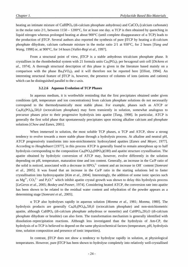
Chapter 1. Polylactide Based Bio-Materials
- 24 -
heating an intimate mixture of CaHPO4 (di-calcium phosphate anhydrous) and CaCO3 (calcium carbonate)
in the molar ratio 2/1, between 1150 – 1200°C, for at least one day. α TCP is then obtained by quenching in liquid nitrogen whereas prolonged heating at about 900°C (until complete disappearance of α TCP) leads to the production of βTCP. Several authors also reported the synthesis of pure βTCP by heating a di-calcium phosphate dihydrate, calcium carbonate mixture in the molar ratio 2/1 at 930°C, for 2 hours [Yang and
Wang, 1998] or, at 900°C, for 14 hours [Vallet-Regí et al., 1997].
From a structural point of view, βTCP is a stable anhydrous tricalcium phosphate phase. It crystallises in the rhombohedral system with 21 formula units Ca3(PO4)2 per hexagonal unit cell [Dickens et al., 1974]. A thorough structural description of this phase is given in the literature based mainly on a comparison with the phase Ba3(VO4)2 and it will therefore not be reported here [Elliott, 1994]. An interesting structural feature of βTCP is, however, the presence of columns of ions (anions and cations)
which can be distinguished parallel to the c-axis.
3.2.2.6 Aqueous Evolution of TCP Phases
In aqueous medium, it is worthwhile reminding that the first precipitates obtained under given conditions (pH, temperature and ion concentrations) from calcium phosphate solutions do not necessarily correspond to the thermodynamically most stable phase. For example, phases such as ATCP or Ca8H2(PO4)6,5H20 (octocalcium phosphate) may form transiently in solution, somewhat analogous to precursor phases prior to their progressive hydrolysis into apatite [Tung, 1998]. In particular, ATCP is generally the first solid phase that spontaneously precipitates upon mixing alkaline calcium and phosphate
solutions [Chow and Eanes, 2001].
When immersed in solution, the most soluble TCP phases, α TCP and ATCP, show a strong tendency to evolve towards a more stable phase through a hydrolysis process. At alkaline and neutral pH, ATCP progressively transforms into non-stoichiometric hydroxylated apatites [Eanes and Meyer, 1977]. According to Heughebaert [1977], in this process ATCP is generally found to remain amorphous up to half hydrolysis corresponding to the composition Ca9(PO4)5(HPO4)(OH) and apatite structure crystallisation. The apatite obtained by hydrolytic conversion of ATCP may, however, evolve differently in the solution depending on pH, temperature, maturation time and ion content. Generally, an increase in the Ca/P ratio of the solid is noticed, associated with a decrease in HPO4
2− content and an increase in OH− content [Somrani et al., 2005]. It was found that an increase in the Ca/P ratio in the starting solutions led to faster crystallisation into hydroxyapatite [Kim et al., 2004]. Interestingly, the addition of some ionic species such as Mg2+, CO3
2−, and P2O74− which inhibit apatite crystal growth was shown to delay this hydrolysis process
[LeGeros et al., 2005; Boskey and Posner, 1974]. Considering heated ATCP, the conversion rate into apatite has been shown to be related to the residual water content and rehydration of the powder appears as a
determining stage [Somrani et al., 2005].
α TCP also hydrolyses rapidly in aqueous solution [Monma et al., 1981; Monma, 1980]. The hydrolysis products are generally Ca8H2(PO4)6,5H20 (octocalcium phosphate) and non-stoichiometric apatite, although CaHPO4 (di-calcium phosphate anhydrous or monetite) and CaHPO4,2H2O (di-calcium phosphate dihydrate or brushite) can also form. The transformation mechanism is generally identified with dissolution–reprecipitation reactions. Although less investigated than the hydrolysis of Am-CP, the hydrolysis of α-TCP is believed to depend on the same physicochemical factors (temperature, pH, hydrolysis
time, solution composition and presence of ionic impurities).
In contrast, βTCP does not show a tendency to hydrolyse rapidly in solution, at physiological temperatures. However, pure βTCP has been shown to hydrolyse completely into relatively well-crystallised
Chapter 1. Polylactide Based Bio-Materials
- 25 -
non-stoichiometric apatitic phases in boiling aqueous suspensions within 24 hours [Rey, 1984]. Faster hydrolysis of βTCP into apatite also occurs under hydrothermal conditions (e.g. 120°C, in the presence of water vapour). These reactions have been found to depend strongly on the purity of βTCP as they are
strongly inhibited in the presence of traces of Mg2+ ions.
3.2.2.7 Surface Properties
Although the understanding of surface interactions between biomaterials and body fluids is of utmost importance for following bio-integration and bioactivity, few data are available to date on the surface
properties of TCP phases, despite their high involvement in the biomaterials field.
Among the indications reported in the literature concerning the surface properties or reactivity of tri-calcium phosphates, most deal either with adsorption or ion exchange processes. However, elucidation of the corresponding mechanisms and the relationship with intrinsic surface properties of the TCP phases
involved, are only rarely addressed.
Adsorption of recombinant human transforming growth factor-β1 on tricalcium phosphate-coated titanium-based implants has been investigated in dogs [Lind et al., 2001]. In this article, authors pointed out a clear increase in the bone volume formed around the implant coated with TCP with adsorbed recombinant human transforming growth factor-β1, thus showing the potential importance of adsorption phenomena on TCP phases. Adsorption of various proteins on βTCP and other calcium phosphates has been investigated by Ohta et al., [2001]. Two kinds of adsorption sites were distinguished: positively charged sites (Ca sites) capable of adsorbing acidic proteins (e.g. bovine serum albumin,) and negatively charged sites (P sites) which adsorb alkaline proteins. Also, the total number of calcium sites on βTCP was then found to be
significantly lower than on the other calcium phosphates tested, including hydroxyapatite.
3.2.3 Application of and -tricalcium Phosphates in Biomaterials
Macro-porous composite scaffolds can be processed using different methods: solvent casting/particulate leaching, emulsion freeze drying or thermally induced phase separation. Biodegradable composite including resorbable polymer such as polylactic acid (PLA) and/or polyglycolic acid (PGA) and a resorbable apatite can be prepared at ambient temperature [Chen et al., 2001a; Linhart et al., 2001]. Recently, Mathieu et al. [2006] reported the use of a supercritical CO2 foaming process to prepare porous PLA-HAp and/or PLA-TCP composites exhibiting mechanical behaviour analogous to bone (anisotropy in
compressive and viscoelastic properties).
Finally, the formation of a polymer-apatite composite can also correspond to a first step in the preparation of nano-crystalline apatite porous ceramic. For example, Tadic et al. [2004] reported the processing of nano-crystalline apatites-based biomaterials porous bio-ceramics using both sodium chloride
salt and polyvinyl alcohol fibres as water-soluble pore agents and cold isostatic pressing without sintering.
4 Conclusion
In this chapter, we have discussed extensively different types of polymers to be used for composite materials with different industrial applications, then application of polymers with different types of fillers and surface modifiers for tissue and bone engineering. The physical, mechanical and thermal properties have been under consideration as they have great impact on the resulting product. Biodegradable polymers from renewable resources have been attracting ever-increasing attention over the past two decades, predominantly for two reasons: the first being environmental concerns and the second being the realization that our petroleum resources are finite. Biodegradable polymers and their products will play an important

Chapter 1. Polylactide Based Bio-Materials
- 26 -
role for transplantation in the coming era. Polylactides are currently used in a number of biomedical applications, such as sutures, stents, dialysis media and drug delivery devices. Also polylactides are used for tissue, cartilage and bone regeneration. Hyaluronic acid is hydrophilic in nature and using it with polylactide will enhance the surface adhesion property of the scaffold produced. As a result it will augment the adhesion, differentiation and proliferation of human cell on the scaffold to be transplanted. Tri-calcium phosphate is added as mineral in the polymer matrix to increase the mechanical properties of the scaffold. The percentage of TCP added depends upon the nature and mechanical property of scaffold required to be
transplanted.
- 27 -
Chapter 2
Chapter 2
Processes to Manufacture Foams and to Functionalize
the Surface
Tissue engineering offers an alternative technique to tissue transplantation for diseased or malfunctioned organs. Adequate porosity and equivalent pore size as well as interconnected pore structure are crucial to allow for easy dispersion of cells throughout the scaffold structure. Scaffold structure is directly related to fabrication methods, which are presented in this chapter one by one. We adopted the technique using supercritical CO2 in our experiments. This process is a green technology which provides adequate porosity and pore size with no loss of bioactive mass in the scaffold matrix. The surface and mechanical properties of the scaffold will be enhanceed by adapting the mixing and co-grinding of polymer matrix with surface modifier and filler. Hyaluronic acid (HA) has a number of potential biomedical applications in drug delivery and tissue engineering. By co-grinding, it coats the surface of polylactide and being hydrophilic in nature thus improves the adhesion energy of the polymer matrix. Similarly filler having
higher mecahnical properties than polymer enhance the modulus and strength of matrix.
1 Generalities on Polymer Foams
The production of polymeric-foam materials can be carried out by either mechanical, chemical, or
physical means. Some of the most commonly used methods are the following [Landrock, 1995]:
Thermal decomposition of chemical blowing agents generating either nitrogen or carbon dioxide, or both, by application of heat, or as the result of the exothermic heat of reaction during polymerization.
Mechanical whipping of gases (frothing) into a polymer system (melt, solution or suspension) which hardens, either by catalytic action or heat, or both, thus entrapping the gas bubbles in the polymer
matrix.
Volatilization of low-boiling liquids such as fluorocarbons or methylene chloride within the polymer mass as the result of the exothermic heat of reaction, or by application of heat.
Volatilization of gases produced by the exothermic heat of reaction during polymerization such as occurs in the reaction of isocyanate with water to form carbon dioxide.
Chapter 2. Processes to Manufacture Foams and to Functionalize the Surface
- 28 -
Expansion of dissolved gas in a polymer mass on reduction of pressure in the system.
Incorporation of hollow microspheres into a polymer mass. The microspheres may consist of either
hollow glass or hollow plastic beads or salts.
Expansion of gas-filled beads by application of heat or expansion of these beads in a polymer mass by the heat of reaction, e.g. expansion of polystyrene beads in a polyurethane or epoxy resin system.
The production of foams can take place by many different techniques. These may include
[Landrock, 1995]:
Continuous slab-stock production by pouring or impingement, using multi-component foam machines.
Compression molding of foams.
Reaction-injection molding (RIM), usually by impingement.
Foaming-in-place by pouring from a dual- or multi-component head.
Spraying of foams.
Extrusion of foams using expandable beads or pellets.
Injection molding of expandable beads or pellets.
Rotational casting of foams.
Frothing of foams, either by introduction of air or of a low-boiling volatile solvent (e.g.
dichlorodifluoromethane, F-12).
Lamination of foams (foam-board production).
Production of foam composites.
Precipitation foam processes where a polymer phase is formed by polymerization or precipitation from a liquid which is later allowed to escape.
2 Manufacturing of Porous Materials by Wet Methods
An ideal scaffold should be biocompatible, biodegradable, and highly porous with interconnected
pores with adequate mechanical properties depending upon the application.
2.1 Solvent Casting/Particulate Leaching
To prepare three-dimensional biodegradable porous scaffolds, a method that incorporates salt particles as the porogen material can be used [Ma and Choi, 2001; Mikos et al., 1994]. The porogen leaching method provides easy control of the pore structure. The pore structure, porosity, and pore size can be easily controlled by regulating the amount and size of salt. This method involves casting a mixture of polymer solution (polymer/chloroform or polymer/methylene chloride) and porogen in a mould, and then leaching out the porogen with water to generate the pores and freeze-drying the mixture. Water-soluble particulates, such as salts and carbohydrates, are used as the porogen materials. Solvent casting / particulate leaching
(SC/PL) involves the use of water-soluble porogen, such as gelatine microspheres or sodium chloride.
The procedure is shown in Figure 2.1 and is applied as follows [Devin et al., 1996; Mooney et al.,
1995; Mikos et al., 1994]:

Chapter 2. Processes to Manufacture Foams and to Functionalize the Surface
- 29 -
(a) Salt particulates are prepared by sieving. The sizes of the salt particulates are controlled by the
desirable sieving.
(b) Polymer solutions are prepared by dissolving different amounts and types of polymers in solvent
(e.g. methylene chloride or chloroform).
(c) Sieved salt particulates are added to the polymer solution, and the dispersion is gently vortexed.
(d) The solution is poured into the designed silicon mould.
(e) Subsequently, the mould with dispersion is pressed (~ 6 MPa) by pressure apparatus.
(f) The formed samples are taken out of the mould.
(g) Samples are dissolved for a desirable time (48 h) in deionised water.
(h) Salt-removed samples are freeze-dried for a desirable time (about 48 h) at low temperature and
reduced pressure (around 8 Pa,−55°C).
(i) The scaffolds are dried in a vacuum oven at 25°C for 1 week to remove the residual solvent.
Scaffolds are kept under vacuum until use.
Figure 2.1: Procedure of solvent casting/particulate leaching. [Khang et al., 2007]
Porosity is independent of particle diameters, but increases with the quantity of salt. A minimum of 70% of salt particles is needed to create interconnected pores [Mikos et al., 1994]. When particle diameter increases, pore size increases. Mechanical properties, such as compressive strength or modulus, are independent of pore size but decrease when porosity increases. Porosity up to 90-95%, with varying pore size, and a compressive modulus of 0.15 to 150 MPa, depending on porosity can be achieved. This method is only applicable to the preparation of thin films since all the salt particles on the bulk must be leached out completely. To obtain thicker scaffolds of desired shape, an improved porogen salt-leaching technique has been proposed [Gross and Rodríguez-Lorenzo, 2004]. By adding small hydroxyapatite (HAp) fibres to a PLGA solution, it is possible to create composite foams with a controlled porosity [Hou et al., 2003; Chen et
al., 2001b; Thomson et al., 1998; Widmer et al., 1998].
2.2 Ice Particle-Leaching
Previous scaffold manufacturing usually involves (1) dissolving the polymer in organic solvent, (2) incorporating porogens, and (3) leaching porogens. Despite these advantages, the problem of residual
(a) Salt (b) Preparing of polymer, solvent, salt
(c) Mixing of polymer, solvent, salt
(d) Moulding (e) Pressing
(f) Removal from (g) Dissolution of salt (h) Freezing & freeze drying
(i) Removal of residual solvent and storage
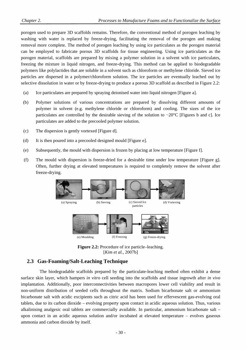
Chapter 2. Processes to Manufacture Foams and to Functionalize the Surface
- 30 -
porogen used to prepare 3D scaffolds remains. Therefore, the conventional method of porogen leaching by washing with water is replaced by freeze-drying, facilitating the removal of the porogen and making removal more complete. The method of porogen leaching by using ice particulates as the porogen material can be employed to fabricate porous 3D scaffolds for tissue engineering. Using ice particulates as the porogen material, scaffolds are prepared by mixing a polymer solution in a solvent with ice particulates, freezing the mixture in liquid nitrogen, and freeze-drying. This method can be applied to biodegradable polymers like polylactides that are soluble in a solvent such as chloroform or methylene chloride. Sieved ice particles are dispersed in a polymer/chloroform solution. The ice particles are eventually leached out by
selective dissolution in water or by freeze-drying to produce a porous 3D scaffold as described in Figure 2.2:
(a) Ice particulates are prepared by spraying deionised water into liquid nitrogen [Figure a].
(b) Polymer solutions of various concentrations are prepared by dissolving different amounts of polymer in solvent (e.g. methylene chloride or chloroform) and cooling. The sizes of the ice particulates are controlled by the desirable sieving of the solution to −20°C [Figures b and c]. Ice
particulates are added to the precooled polymer solution.
(c) The dispersion is gently vortexed [Figure d].
(d) It is then poured into a precooled designed mould [Figure e].
(e) Subsequently, the mould with dispersion is frozen by placing at low temperature [Figure f].
(f) The mould with dispersion is freeze-dried for a desirable time under low temperature [Figure g]. Often, further drying at elevated temperatures is required to completely remove the solvent after
freeze-drying.
Figure 2.2: Procedure of ice particle–leaching. [Kim et al., 2007b]
2.3 Gas-Foaming/Salt-Leaching Technique
The biodegradable scaffolds prepared by the particulate-leaching method often exhibit a dense surface skin layer, which hampers in vitro cell seeding into the scaffolds and tissue ingrowth after in vivo implantation. Additionally, poor interconnectivities between macropores lower cell viability and result in non-uniform distribution of seeded cells throughout the matrix. Sodium bicarbonate salt or ammonium bicarbonate salt with acidic excipients such as citric acid has been used for effervescent gas-evolving oral tablets, due to its carbon dioxide – evolving property upon contact in acidic aqueous solution. Thus, various alkalinising analgesic oral tablets are commercially available. In particular, ammonium bicarbonate salt – upon contact in an acidic aqueous solution and/or incubated at elevated temperature – evolves gaseous
ammonia and carbon dioxide by itself.
(a) Spraying (b) Sieving (c) Sieved Ice particles
(d) Vortexing
(e) Moulding (f) Freezing (g) Freeze-drying
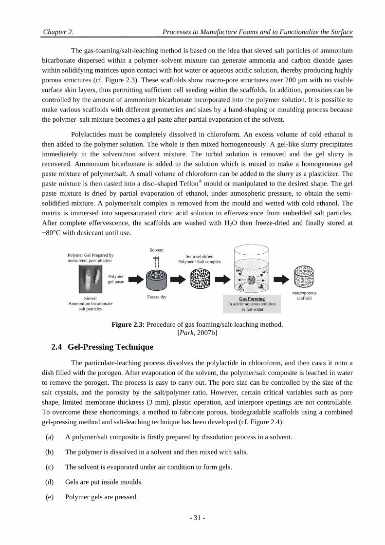
Chapter 2. Processes to Manufacture Foams and to Functionalize the Surface
- 31 -
The gas-foaming/salt-leaching method is based on the idea that sieved salt particles of ammonium bicarbonate dispersed within a polymer–solvent mixture can generate ammonia and carbon dioxide gases within solidifying matrices upon contact with hot water or aqueous acidic solution, thereby producing highly porous structures (cf. Figure 2.3). These scaffolds show macro-pore structures over 200 μm with no visible surface skin layers, thus permitting sufficient cell seeding within the scaffolds. In addition, porosities can be controlled by the amount of ammonium bicarbonate incorporated into the polymer solution. It is possible to make various scaffolds with different geometries and sizes by a hand-shaping or moulding process because
the polymer–salt mixture becomes a gel paste after partial evaporation of the solvent.
Polylactides must be completely dissolved in chloroform. An excess volume of cold ethanol is then added to the polymer solution. The whole is then mixed homogeneously. A gel-like slurry precipitates immediately in the solvent/non solvent mixture. The turbid solution is removed and the gel slurry is recovered. Ammonium bicarbonate is added to the solution which is mixed to make a homogeneous gel paste mixture of polymer/salt. A small volume of chloroform can be added to the slurry as a plasticizer. The paste mixture is then casted into a disc–shaped Teflon® mould or manipulated to the desired shape. The gel paste mixture is dried by partial evaporation of ethanol, under atmospheric pressure, to obtain the semi-solidified mixture. A polymer/salt complex is removed from the mould and wetted with cold ethanol. The matrix is immersed into supersaturated citric acid solution to effervescence from embedded salt particles. After complete effervescence, the scaffolds are washed with H2O then freeze-dried and finally stored at
−80°C with desiccant until use.
Figure 2.3: Procedure of gas foaming/salt-leaching method. [Park, 2007b]
2.4 Gel-Pressing Technique
The particulate-leaching process dissolves the polylactide in chloroform, and then casts it onto a dish filled with the porogen. After evaporation of the solvent, the polymer/salt composite is leached in water to remove the porogen. The process is easy to carry out. The pore size can be controlled by the size of the salt crystals, and the porosity by the salt/polymer ratio. However, certain critical variables such as pore shape, limited membrane thickness (3 mm), plastic operation, and interpore openings are not controllable. To overcome these shortcomings, a method to fabricate porous, biodegradable scaffolds using a combined
gel-pressing method and salt-leaching technique has been developed (cf. Figure 2.4):
(a) A polymer/salt composite is firstly prepared by dissolution process in a solvent.
(b) The polymer is dissolved in a solvent and then mixed with salts.
(c) The solvent is evaporated under air condition to form gels.
(d) Gels are put inside moulds.
(e) Polymer gels are pressed.
Polymer Gel Prepared by nonsolvent precipitation
Sieved Ammonium bicarbonate
salt particles
Polymer gel paste
Macroporous scaffold Gas Forming
In acidic aqueous solution or hot water
Freeze dry
Solvent
Semi solidified Polymer / Salt complex
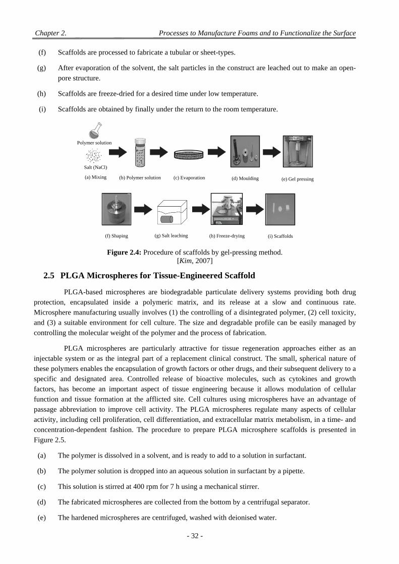
Chapter 2. Processes to Manufacture Foams and to Functionalize the Surface
- 32 -
(f) Scaffolds are processed to fabricate a tubular or sheet-types.
(g) After evaporation of the solvent, the salt particles in the construct are leached out to make an open-
pore structure.
(h) Scaffolds are freeze-dried for a desired time under low temperature.
(i) Scaffolds are obtained by finally under the return to the room temperature.
Figure 2.4: Procedure of scaffolds by gel-pressing method. [Kim, 2007]
2.5 PLGA Microspheres for Tissue-Engineered Scaffold
PLGA-based microspheres are biodegradable particulate delivery systems providing both drug protection, encapsulated inside a polymeric matrix, and its release at a slow and continuous rate. Microsphere manufacturing usually involves (1) the controlling of a disintegrated polymer, (2) cell toxicity, and (3) a suitable environment for cell culture. The size and degradable profile can be easily managed by
controlling the molecular weight of the polymer and the process of fabrication.
PLGA microspheres are particularly attractive for tissue regeneration approaches either as an injectable system or as the integral part of a replacement clinical construct. The small, spherical nature of these polymers enables the encapsulation of growth factors or other drugs, and their subsequent delivery to a specific and designated area. Controlled release of bioactive molecules, such as cytokines and growth factors, has become an important aspect of tissue engineering because it allows modulation of cellular function and tissue formation at the afflicted site. Cell cultures using microspheres have an advantage of passage abbreviation to improve cell activity. The PLGA microspheres regulate many aspects of cellular activity, including cell proliferation, cell differentiation, and extracellular matrix metabolism, in a time- and concentration-dependent fashion. The procedure to prepare PLGA microsphere scaffolds is presented in
Figure 2.5.
(a) The polymer is dissolved in a solvent, and is ready to add to a solution in surfactant.
(b) The polymer solution is dropped into an aqueous solution in surfactant by a pipette.
(c) This solution is stirred at 400 rpm for 7 h using a mechanical stirrer.
(d) The fabricated microspheres are collected from the bottom by a centrifugal separator.
(e) The hardened microspheres are centrifuged, washed with deionised water.
Salt (NaCl)
(a) Mixing (b) Polymer solution (c) Evaporation (d) Moulding (e) Gel pressing
(f) Shaping (g) Salt leaching (h) Freeze-drying (i) Scaffolds
Polymer solution
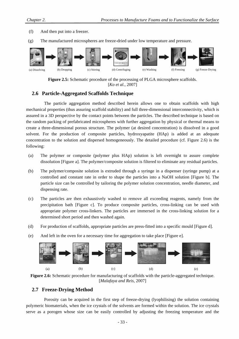
Chapter 2. Processes to Manufacture Foams and to Functionalize the Surface
- 33 -
(f) And then put into a freezer.
(g) The manufactured microspheres are freeze-dried under low temperature and pressure.
Figure 2.5: Schematic procedure of the processing of PLGA microsphere scaffolds. [Ko et al., 2007]
2.6 Particle-Aggregated Scaffolds Technique
The particle aggregation method described herein allows one to obtain scaffolds with high mechanical properties (thus assuring scaffold stability) and full three-dimensional interconnectivity, which is assured in a 3D perspective by the contact points between the particles. The described technique is based on the random packing of prefabricated microspheres with further aggregation by physical or thermal means to create a three-dimensional porous structure. The polymer (at desired concentration) is dissolved in a good solvent. For the production of composite particles, hydroxyapatite (HAp) is added at an adequate concentration to the solution and dispersed homogeneously. The detailed procedure (cf. Figure 2.6) is the
following:
(a) The polymer or composite (polymer plus HAp) solution is left overnight to assure complete
dissolution [Figure a]. The polymer/composite solution is filtered to eliminate any residual particles.
(b) The polymer/composite solution is extruded through a syringe in a dispenser (syringe pump) at a controlled and constant rate in order to shape the particles into a NaOH solution [Figure b]. The particle size can be controlled by tailoring the polymer solution concentration, needle diameter, and
dispensing rate.
(c) The particles are then exhaustively washed to remove all exceeding reagents, namely from the precipitation bath [Figure c]. To produce composite particles, cross-linking can be used with appropriate polymer cross-linkers. The particles are immersed in the cross-linking solution for a
determined short period and then washed again.
(d) For production of scaffolds, appropriate particles are press-fitted into a specific mould [Figure d].
(e) And left in the oven for a necessary time for aggregation to take place [Figure e].
Figure 2.6: Schematic procedure for manufacturing of scaffolds with the particle-aggregated technique.
[Malafaya and Reis, 2007]
2.7 Freeze-Drying Method
Porosity can be acquired in the first step of freeze-drying (lyophilising) the solution containing polymeric biomaterials, when the ice crystals of the solvents are formed within the solution. The ice crystals serve as a porogen whose size can be easily controlled by adjusting the freezing temperature and the
(a) (b) (c) (d) (e)
(a) Dissolving (b) Dropping (c) Stirring (d) Centrifuging (e) Washing (f) Freezing (g) Freeze-Drying
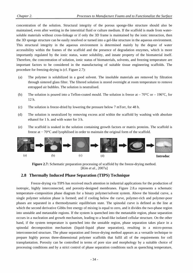
Chapter 2. Processes to Manufacture Foams and to Functionalize the Surface
- 34 -
concentration of the solution. Structural integrity of the porous sponge-like structure should also be maintained, even after wetting in the interstitial fluid or culture medium. If the scaffold is made from water-soluble materials without cross-linkage or if only the 3D frame is maintained by the ionic interaction, then the 3D sponge structure can be easily resolved or turned into a gel-like structure in the aqueous environment. This structural integrity in the aqueous environment is determined mainly by the degree of water accessibility within the frames of the scaffold and the presence of degradation enzymes, which is more importantly regulated by the ionic status, water solubility, and innate property of the biomaterial itself. Therefore, the concentration of solution, ionic status of biomaterials, solvents, and freezing temperature are important factors to be considered in the manufacturing of suitable tissue engineering scaffolds. The
procedure for freezing-drying is (cf. Figure 2.7):
(a) The polymer is solubilized in a good solvent. The insoluble materials are removed by filtration through sintered glass filter. The filtered solution is stored overnight at room temperature to remove
entrapped air bubbles. The solution is neutralised.
(b) The solution is poured into a Teflon-coated mould. The solution is freeze at – 70°C or – 196°C, for
12 h.
(c) The solution is freeze-dried by lowering the pressure below 7 mTorr, for 48 h.
(d) The solution is neutralized by removing excess acid within the scaffold by washing with absolute
ethanol for 1 h. and with water for 3 h.
(e) The scaffold is soaked in the solution containing growth factors or matrix proteins. The scaffold is
freeze at − 70°C and lyophilised in order to maintain the original form of the scaffold.
Figure 2.7: Schematic preparation processing of scaffold by the freeze-drying method. [Kim et al., 2007a]
2.8 Thermally Induced Phase Separation (TIPS) Technique
Freeze-drying via TIPS has received much attention in industrial applications for the production of isotropic, highly interconnected, and porosity-designed membranes. Figure 2.8.a represents a schematic temperature–composition phase diagram for a binary polymer/solvent system. Above the binodal curve, a single polymer solution phase is formed; and if cooling below the curve, polymer-rich and polymer-poor phases are separated in a thermodynamic equilibrium state. The spinodal curve is defined as the line at which the second derivative Gibbs free energy of mixing is equal to zero, and it divides the two-phase region into unstable and metastable regions. If the system is quenched into the metastable region, phase separation occurs in a nucleation and growth mechanism, leading to a bead-like isolated cellular structure. On the other hand, if the system temperature is quenched into the unstable region, phase separation takes place in a spinodal decomposition mechanism (liquid–liquid phase separation), resulting in a micro-porous interconnected structure. The phase separation and freeze-drying method appears as a versatile technique to prepare highly porous three-dimensional polymer scaffolds that fulfil all of the requirements for cell transplantation. Porosity can be controlled in terms of pore size and morphology by a suitable choice of processing conditions and by a strict control of phase separation conditions such as quenching temperature,
(a) (b) (c) (d) Introduc
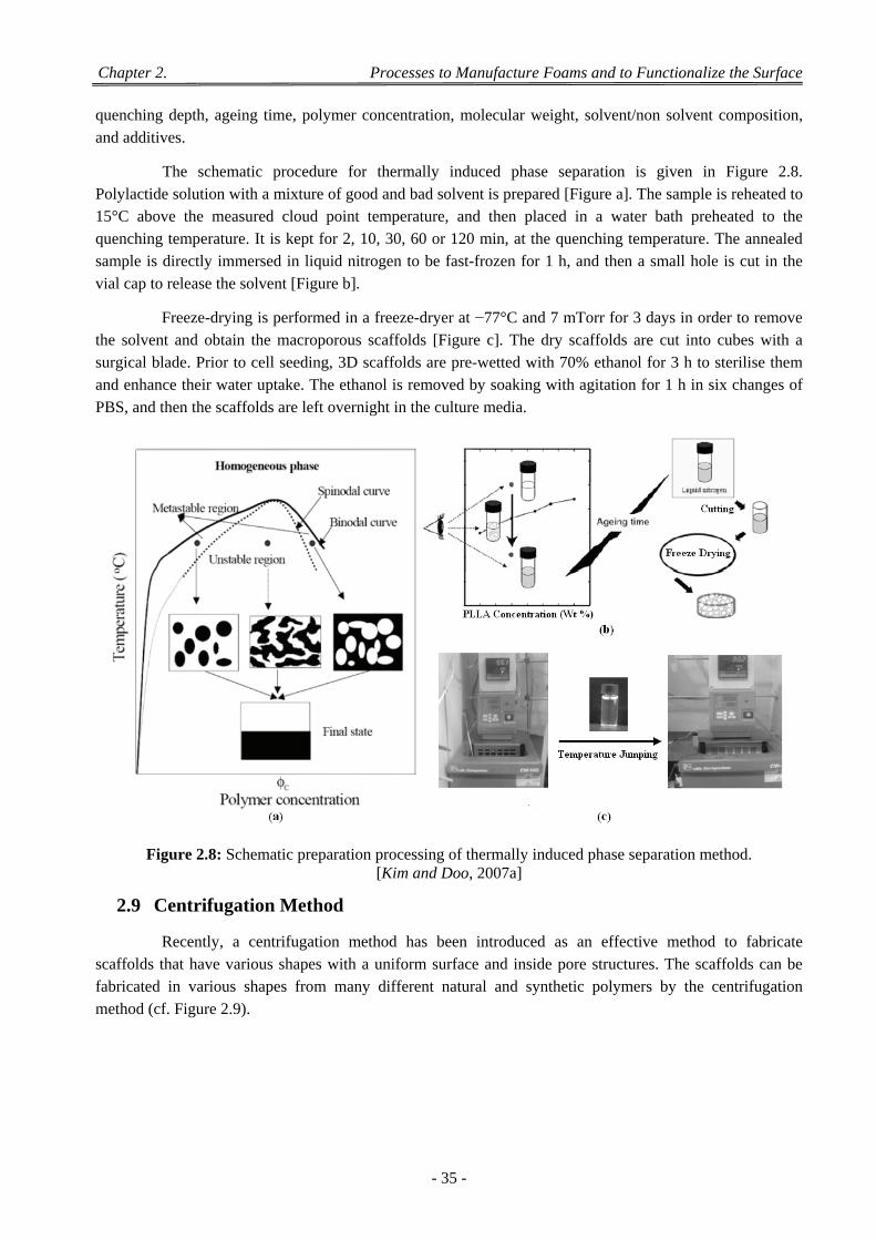
Chapter 2. Processes to Manufacture Foams and to Functionalize the Surface
- 35 -
quenching depth, ageing time, polymer concentration, molecular weight, solvent/non solvent composition,
and additives.
The schematic procedure for thermally induced phase separation is given in Figure 2.8. Polylactide solution with a mixture of good and bad solvent is prepared [Figure a]. The sample is reheated to 15°C above the measured cloud point temperature, and then placed in a water bath preheated to the quenching temperature. It is kept for 2, 10, 30, 60 or 120 min, at the quenching temperature. The annealed sample is directly immersed in liquid nitrogen to be fast-frozen for 1 h, and then a small hole is cut in the
vial cap to release the solvent [Figure b].
Freeze-drying is performed in a freeze-dryer at −77°C and 7 mTorr for 3 days in order to remove the solvent and obtain the macroporous scaffolds [Figure c]. The dry scaffolds are cut into cubes with a surgical blade. Prior to cell seeding, 3D scaffolds are pre-wetted with 70% ethanol for 3 h to sterilise them and enhance their water uptake. The ethanol is removed by soaking with agitation for 1 h in six changes of
PBS, and then the scaffolds are left overnight in the culture media.
Figure 2.8: Schematic preparation processing of thermally induced phase separation method. [Kim and Doo, 2007a]
2.9 Centrifugation Method
Recently, a centrifugation method has been introduced as an effective method to fabricate scaffolds that have various shapes with a uniform surface and inside pore structures. The scaffolds can be fabricated in various shapes from many different natural and synthetic polymers by the centrifugation
method (cf. Figure 2.9).
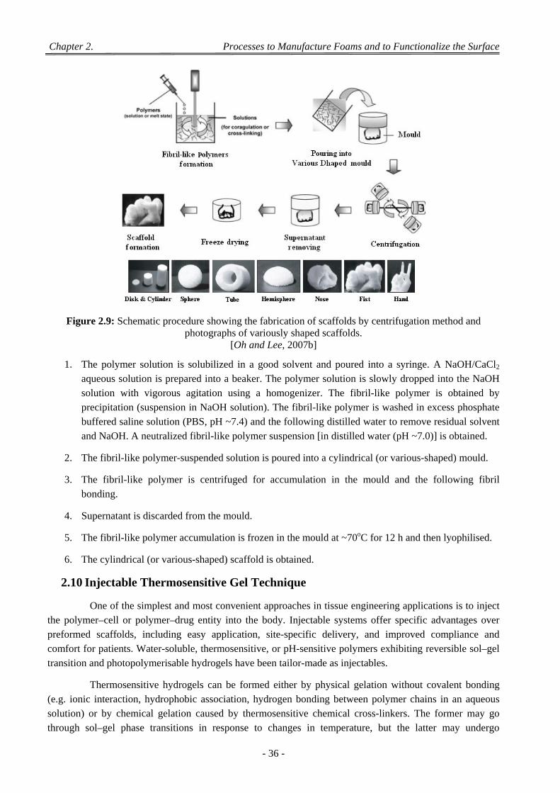
Chapter 2. Processes to Manufacture Foams and to Functionalize the Surface
- 36 -
Figure 2.9: Schematic procedure showing the fabrication of scaffolds by centrifugation method and photographs of variously shaped scaffolds.
[Oh and Lee, 2007b]
1. The polymer solution is solubilized in a good solvent and poured into a syringe. A NaOH/CaCl2 aqueous solution is prepared into a beaker. The polymer solution is slowly dropped into the NaOH solution with vigorous agitation using a homogenizer. The fibril-like polymer is obtained by precipitation (suspension in NaOH solution). The fibril-like polymer is washed in excess phosphate buffered saline solution (PBS, pH ~7.4) and the following distilled water to remove residual solvent
and NaOH. A neutralized fibril-like polymer suspension [in distilled water (pH ~7.0)] is obtained.
2. The fibril-like polymer-suspended solution is poured into a cylindrical (or various-shaped) mould.
3. The fibril-like polymer is centrifuged for accumulation in the mould and the following fibril
bonding.
4. Supernatant is discarded from the mould.
5. The fibril-like polymer accumulation is frozen in the mould at ~70oC for 12 h and then lyophilised.
6. The cylindrical (or various-shaped) scaffold is obtained.
2.10 Injectable Thermosensitive Gel Technique
One of the simplest and most convenient approaches in tissue engineering applications is to inject the polymer–cell or polymer–drug entity into the body. Injectable systems offer specific advantages over preformed scaffolds, including easy application, site-specific delivery, and improved compliance and comfort for patients. Water-soluble, thermosensitive, or pH-sensitive polymers exhibiting reversible sol–gel
transition and photopolymerisable hydrogels have been tailor-made as injectables.
Thermosensitive hydrogels can be formed either by physical gelation without covalent bonding (e.g. ionic interaction, hydrophobic association, hydrogen bonding between polymer chains in an aqueous solution) or by chemical gelation caused by thermosensitive chemical cross-linkers. The former may go through sol–gel phase transitions in response to changes in temperature, but the latter may undergo
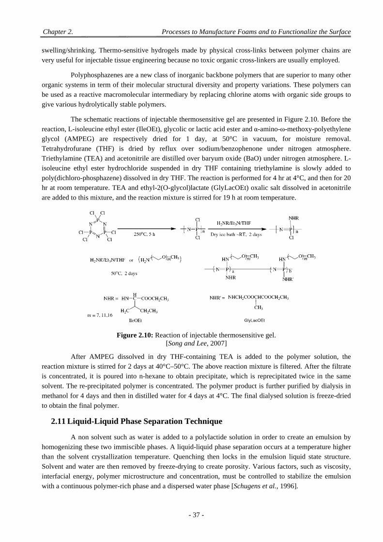
Chapter 2. Processes to Manufacture Foams and to Functionalize the Surface
- 37 -
swelling/shrinking. Thermo-sensitive hydrogels made by physical cross-links between polymer chains are
very useful for injectable tissue engineering because no toxic organic cross-linkers are usually employed.
Polyphosphazenes are a new class of inorganic backbone polymers that are superior to many other organic systems in term of their molecular structural diversity and property variations. These polymers can be used as a reactive macromolecular intermediary by replacing chlorine atoms with organic side groups to
give various hydrolytically stable polymers.
The schematic reactions of injectable thermosensitive gel are presented in Figure 2.10. Before the reaction, L-isoleucine ethyl ester (IleOEt), glycolic or lactic acid ester and α-amino-ω-methoxy-polyethylene glycol (AMPEG) are respectively dried for 1 day, at 50°C in vacuum, for moisture removal. Tetrahydrofurane (THF) is dried by reflux over sodium/benzophenone under nitrogen atmosphere. Triethylamine (TEA) and acetonitrile are distilled over baryum oxide (BaO) under nitrogen atmosphere. L-isoleucine ethyl ester hydrochloride suspended in dry THF containing triethylamine is slowly added to poly(dichloro-phosphazene) dissolved in dry THF. The reaction is performed for 4 hr at 4°C, and then for 20 hr at room temperature. TEA and ethyl-2(O-glycol)lactate (GlyLacOEt) oxalic salt dissolved in acetonitrile
are added to this mixture, and the reaction mixture is stirred for 19 h at room temperature.
Figure 2.10: Reaction of injectable thermosensitive gel. [Song and Lee, 2007]
After AMPEG dissolved in dry THF-containing TEA is added to the polymer solution, the reaction mixture is stirred for 2 days at 40°C–50°C. The above reaction mixture is filtered. After the filtrate is concentrated, it is poured into n-hexane to obtain precipitate, which is reprecipitated twice in the same solvent. The re-precipitated polymer is concentrated. The polymer product is further purified by dialysis in methanol for 4 days and then in distilled water for 4 days at 4°C. The final dialysed solution is freeze-dried
to obtain the final polymer.
2.11 Liquid-Liquid Phase Separation Technique
A non solvent such as water is added to a polylactide solution in order to create an emulsion by homogenizing these two immiscible phases. A liquid-liquid phase separation occurs at a temperature higher than the solvent crystallization temperature. Quenching then locks in the emulsion liquid state structure. Solvent and water are then removed by freeze-drying to create porosity. Various factors, such as viscosity, interfacial energy, polymer microstructure and concentration, must be controlled to stabilize the emulsion
with a continuous polymer-rich phase and a dispersed water phase [Schugens et al., 1996].
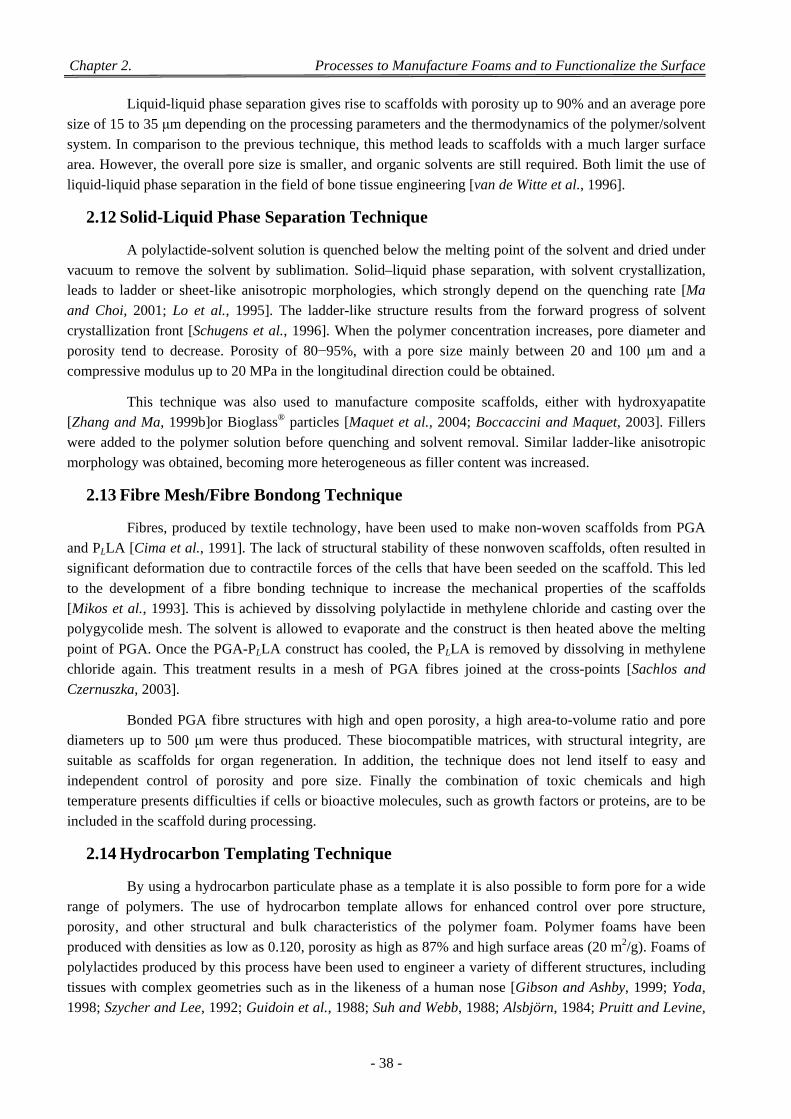
Chapter 2. Processes to Manufacture Foams and to Functionalize the Surface
- 38 -
Liquid-liquid phase separation gives rise to scaffolds with porosity up to 90% and an average pore size of 15 to 35 μm depending on the processing parameters and the thermodynamics of the polymer/solvent system. In comparison to the previous technique, this method leads to scaffolds with a much larger surface area. However, the overall pore size is smaller, and organic solvents are still required. Both limit the use of
liquid-liquid phase separation in the field of bone tissue engineering [van de Witte et al., 1996].
2.12 Solid-Liquid Phase Separation Technique
A polylactide-solvent solution is quenched below the melting point of the solvent and dried under vacuum to remove the solvent by sublimation. Solid–liquid phase separation, with solvent crystallization, leads to ladder or sheet-like anisotropic morphologies, which strongly depend on the quenching rate [Ma and Choi, 2001; Lo et al., 1995]. The ladder-like structure results from the forward progress of solvent crystallization front [Schugens et al., 1996]. When the polymer concentration increases, pore diameter and porosity tend to decrease. Porosity of 80−95%, with a pore size mainly between 20 and 100 μm and a
compressive modulus up to 20 MPa in the longitudinal direction could be obtained.
This technique was also used to manufacture composite scaffolds, either with hydroxyapatite [Zhang and Ma, 1999b]or Bioglass® particles [Maquet et al., 2004; Boccaccini and Maquet, 2003]. Fillers were added to the polymer solution before quenching and solvent removal. Similar ladder-like anisotropic
morphology was obtained, becoming more heterogeneous as filler content was increased.
2.13 Fibre Mesh/Fibre Bondong Technique
Fibres, produced by textile technology, have been used to make non-woven scaffolds from PGA and PLLA [Cima et al., 1991]. The lack of structural stability of these nonwoven scaffolds, often resulted in significant deformation due to contractile forces of the cells that have been seeded on the scaffold. This led to the development of a fibre bonding technique to increase the mechanical properties of the scaffolds [Mikos et al., 1993]. This is achieved by dissolving polylactide in methylene chloride and casting over the polygycolide mesh. The solvent is allowed to evaporate and the construct is then heated above the melting point of PGA. Once the PGA-PLLA construct has cooled, the PLLA is removed by dissolving in methylene chloride again. This treatment results in a mesh of PGA fibres joined at the cross-points [Sachlos and
Czernuszka, 2003].
Bonded PGA fibre structures with high and open porosity, a high area-to-volume ratio and pore diameters up to 500 μm were thus produced. These biocompatible matrices, with structural integrity, are suitable as scaffolds for organ regeneration. In addition, the technique does not lend itself to easy and independent control of porosity and pore size. Finally the combination of toxic chemicals and high temperature presents difficulties if cells or bioactive molecules, such as growth factors or proteins, are to be
included in the scaffold during processing.
2.14 Hydrocarbon Templating Technique
By using a hydrocarbon particulate phase as a template it is also possible to form pore for a wide range of polymers. The use of hydrocarbon template allows for enhanced control over pore structure, porosity, and other structural and bulk characteristics of the polymer foam. Polymer foams have been produced with densities as low as 0.120, porosity as high as 87% and high surface areas (20 m2/g). Foams of polylactides produced by this process have been used to engineer a variety of different structures, including tissues with complex geometries such as in the likeness of a human nose [Gibson and Ashby, 1999; Yoda, 1998; Szycher and Lee, 1992; Guidoin et al., 1988; Suh and Webb, 1988; Alsbjörn, 1984; Pruitt and Levine,
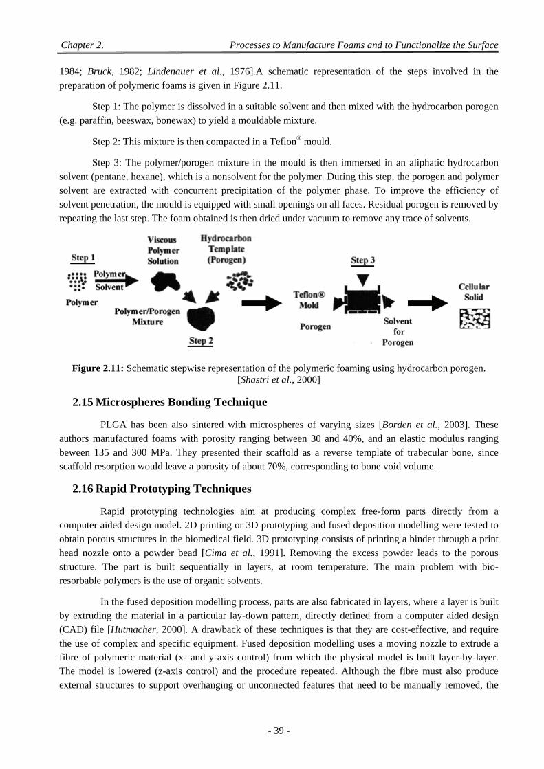
Chapter 2. Processes to Manufacture Foams and to Functionalize the Surface
- 39 -
1984; Bruck, 1982; Lindenauer et al., 1976].A schematic representation of the steps involved in the
preparation of polymeric foams is given in Figure 2.11.
Step 1: The polymer is dissolved in a suitable solvent and then mixed with the hydrocarbon porogen
(e.g. paraffin, beeswax, bonewax) to yield a mouldable mixture.
Step 2: This mixture is then compacted in a Teflon® mould.
Step 3: The polymer/porogen mixture in the mould is then immersed in an aliphatic hydrocarbon solvent (pentane, hexane), which is a nonsolvent for the polymer. During this step, the porogen and polymer solvent are extracted with concurrent precipitation of the polymer phase. To improve the efficiency of solvent penetration, the mould is equipped with small openings on all faces. Residual porogen is removed by
repeating the last step. The foam obtained is then dried under vacuum to remove any trace of solvents.
Figure 2.11: Schematic stepwise representation of the polymeric foaming using hydrocarbon porogen. [Shastri et al., 2000]
2.15 Microspheres Bonding Technique
PLGA has been also sintered with microspheres of varying sizes [Borden et al., 2003]. These authors manufactured foams with porosity ranging between 30 and 40%, and an elastic modulus ranging beween 135 and 300 MPa. They presented their scaffold as a reverse template of trabecular bone, since
scaffold resorption would leave a porosity of about 70%, corresponding to bone void volume.
2.16 Rapid Prototyping Techniques
Rapid prototyping technologies aim at producing complex free-form parts directly from a computer aided design model. 2D printing or 3D prototyping and fused deposition modelling were tested to obtain porous structures in the biomedical field. 3D prototyping consists of printing a binder through a print head nozzle onto a powder bead [Cima et al., 1991]. Removing the excess powder leads to the porous structure. The part is built sequentially in layers, at room temperature. The main problem with bio-resorbable polymers is the use of organic solvents.
In the fused deposition modelling process, parts are also fabricated in layers, where a layer is built by extruding the material in a particular lay-down pattern, directly defined from a computer aided design (CAD) file [Hutmacher, 2000]. A drawback of these techniques is that they are cost-effective, and require the use of complex and specific equipment. Fused deposition modelling uses a moving nozzle to extrude a fibre of polymeric material (x- and y-axis control) from which the physical model is built layer-by-layer. The model is lowered (z-axis control) and the procedure repeated. Although the fibre must also produce external structures to support overhanging or unconnected features that need to be manually removed, the
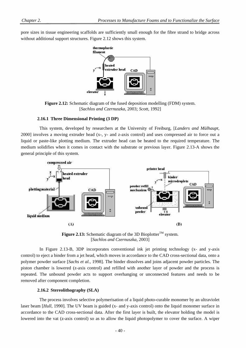
Chapter 2. Processes to Manufacture Foams and to Functionalize the Surface
- 40 -
pore sizes in tissue engineering scaffolds are sufficiently small enough for the fibre strand to bridge across
without additional support structures. Figure 2.12 shows this system.
Figure 2.12: Schematic diagram of the fused deposition modelling (FDM) system. [Sachlos and Czernuszka, 2003; Scott, 1992]
2.16.1 Three Dimensional Printing (3 DP)
This system, developed by researchers at the University of Freiburg, [Landers and Mülhaupt, 2000] involves a moving extruder head (x-, y- and z-axis control) and uses compressed air to force out a liquid or paste-like plotting medium. The extruder head can be heated to the required temperature. The medium solidifies when it comes in contact with the substrate or previous layer. Figure 2.13-A shows the
general principle of this system.
Figure 2.13: Schematic diagram of the 3D BioplotterTM system. [Sachlos and Czernuszka, 2003]
In Figure 2.13-B, 3DP incorporates conventional ink jet printing technology (x- and y-axis control) to eject a binder from a jet head, which moves in accordance to the CAD cross-sectional data, onto a polymer powder surface [Sachs et al., 1998]. The binder dissolves and joins adjacent powder particles. The piston chamber is lowered (z-axis control) and refilled with another layer of powder and the process is repeated. The unbound powder acts to support overhanging or unconnected features and needs to be
removed after component completion.
2.16.2 Stereolithography (SLA)
The process involves selective polymerisation of a liquid photo-curable monomer by an ultraviolet laser beam [Hull, 1990]. The UV beam is guided (x- and y-axis control) onto the liquid monomer surface in accordance to the CAD cross-sectional data. After the first layer is built, the elevator holding the model is lowered into the vat (z-axis control) so as to allow the liquid photopolymer to cover the surface. A wiper
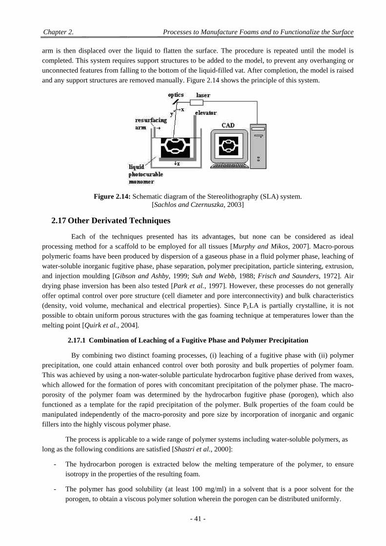
Chapter 2. Processes to Manufacture Foams and to Functionalize the Surface
- 41 -
arm is then displaced over the liquid to flatten the surface. The procedure is repeated until the model is completed. This system requires support structures to be added to the model, to prevent any overhanging or unconnected features from falling to the bottom of the liquid-filled vat. After completion, the model is raised
and any support structures are removed manually. Figure 2.14 shows the principle of this system.
Figure 2.14: Schematic diagram of the Stereolithography (SLA) system. [Sachlos and Czernuszka, 2003]
2.17 Other Derivated Techniques
Each of the techniques presented has its advantages, but none can be considered as ideal processing method for a scaffold to be employed for all tissues [Murphy and Mikos, 2007]. Macro-porous polymeric foams have been produced by dispersion of a gaseous phase in a fluid polymer phase, leaching of water-soluble inorganic fugitive phase, phase separation, polymer precipitation, particle sintering, extrusion, and injection moulding [Gibson and Ashby, 1999; Suh and Webb, 1988; Frisch and Saunders, 1972]. Air drying phase inversion has been also tested [Park et al., 1997]. However, these processes do not generally offer optimal control over pore structure (cell diameter and pore interconnectivity) and bulk characteristics (density, void volume, mechanical and electrical properties). Since PLLA is partially crystalline, it is not possible to obtain uniform porous structures with the gas foaming technique at temperatures lower than the
melting point [Quirk et al., 2004].
2.17.1 Combination of Leaching of a Fugitive Phase and Polymer Precipitation
By combining two distinct foaming processes, (i) leaching of a fugitive phase with (ii) polymer precipitation, one could attain enhanced control over both porosity and bulk properties of polymer foam. This was achieved by using a non-water-soluble particulate hydrocarbon fugitive phase derived from waxes, which allowed for the formation of pores with concomitant precipitation of the polymer phase. The macro-porosity of the polymer foam was determined by the hydrocarbon fugitive phase (porogen), which also functioned as a template for the rapid precipitation of the polymer. Bulk properties of the foam could be manipulated independently of the macro-porosity and pore size by incorporation of inorganic and organic
fillers into the highly viscous polymer phase.
The process is applicable to a wide range of polymer systems including water-soluble polymers, as
long as the following conditions are satisfied [Shastri et al., 2000]:
- The hydrocarbon porogen is extracted below the melting temperature of the polymer, to ensure
isotropy in the properties of the resulting foam.
- The polymer has good solubility (at least 100 mg/ml) in a solvent that is a poor solvent for the
porogen, to obtain a viscous polymer solution wherein the porogen can be distributed uniformly.
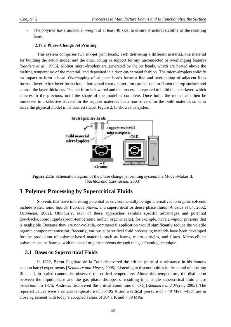
Chapter 2. Processes to Manufacture Foams and to Functionalize the Surface
- 42 -
- The polymer has a molecular weight of at least 40 kDa, to ensure structural stability of the resulting
foam.
2.17.2 Phase-Change Jet Printing
This system comprises two ink-jet print heads; each delivering a different material, one material for building the actual model and the other acting as support for any unconnected or overhanging features [Sanders et al., 1996]. Molten micro-droplets are generated by the jet heads, which are heated above the melting temperature of the material, and deposited in a drop-on-demand fashion. The micro-droplets solidify on impact to form a bead. Overlapping of adjacent beads forms a line and overlapping of adjacent lines forms a layer. After layer formation, a horizontal rotary cutter arm can be used to flatten the top surface and control the layer thickness. The platform is lowered and the process is repeated to build the next layer, which adheres to the previous, until the shape of the model is complete. Once built, the model can then be immersed in a selective solvent for the support material, but a non-solvent for the build material, so as to
leave the physical model in its desired shape. Figure 2.15 shows this system.
Figure 2.15: Schematic diagram of the phase change jet printing system, the Model-Maker II. [Sachlos and Czernuszka, 2003]
3 Polymer Processing by Supercritical Fluids
Solvents that have interesting potential as environmentally benign alternatives to organic solvents include water, ionic liquids, fluorous phases, and supercritical or dense phase fluids [Anastas et al., 2002; DeSimone, 2002]. Obviously, each of these approaches exhibits specific advantages and potential drawbacks. Ionic liquids (room-temperature molten organic salts), for example, have a vapour pressure that is negligible. Because they are non-volatile, commercial application would significantly reduce the volatile organic component emission. Recently, various supercritical fluid processing methods have been developed for the production of polymer-based materials such as foams, micro-particles, and fibres. Microcellular
polymers can be foamed with no use of organic solvents through the gas foaming technique.
3.1 Bases on Supercritical Fluids
In 1822, Baron Cagniard de la Tour discovered the critical point of a substance in his famous cannon barrel experiments [Kemmere and Meyer, 2005]. Listening to discontinuities in the sound of a rolling flint ball, in sealed cannon, he observed the critical temperature. Above this temperature, the distinction between the liquid phase and the gas phase disappears, resulting in a single supercritical fluid phase behaviour. In 1875, Andrews discovered the critical conditions of CO2 [Kemmere and Meyer, 2005]. The reported values were a critical temperature of 304.05 K and a critical pressure of 7.40 MPa, which are in
close agreement with today’s accepted values of 304.1 K and 7.38 MPa.
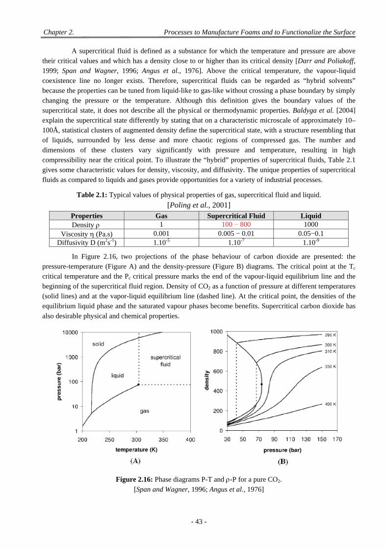
Chapter 2. Processes to Manufacture Foams and to Functionalize the Surface
- 43 -
A supercritical fluid is defined as a substance for which the temperature and pressure are above their critical values and which has a density close to or higher than its critical density [Darr and Poliakoff, 1999; Span and Wagner, 1996; Angus et al., 1976]. Above the critical temperature, the vapour-liquid coexistence line no longer exists. Therefore, supercritical fluids can be regarded as “hybrid solvents” because the properties can be tuned from liquid-like to gas-like without crossing a phase boundary by simply changing the pressure or the temperature. Although this definition gives the boundary values of the supercritical state, it does not describe all the physical or thermodynamic properties. Baldyga et al. [2004] explain the supercritical state differently by stating that on a characteristic microscale of approximately 10–100Å, statistical clusters of augmented density define the supercritical state, with a structure resembling that of liquids, surrounded by less dense and more chaotic regions of compressed gas. The number and dimensions of these clusters vary significantly with pressure and temperature, resulting in high compressibility near the critical point. To illustrate the “hybrid” properties of supercritical fluids, Table 2.1 gives some characteristic values for density, viscosity, and diffusivity. The unique properties of supercritical
fluids as compared to liquids and gases provide opportunities for a variety of industrial processes.
Table 2.1: Typical values of physical properties of gas, supercritical fluid and liquid.
[Poling et al., 2001] Properties Gas Supercritical Fluid Liquid Density 1 100 − 800 1000
Viscosity (Pa.s) 0.001 0.005 − 0.01 0.05−0.1 Diffusivity D (m2s-1) 1.10-5 1.10-7 1.10-9
In Figure 2.16, two projections of the phase behaviour of carbon dioxide are presented: the pressure-temperature (Figure A) and the density-pressure (Figure B) diagrams. The critical point at the Tc critical temperature and the Pc critical pressure marks the end of the vapour-liquid equilibrium line and the beginning of the supercritical fluid region. Density of CO2 as a function of pressure at different temperatures (solid lines) and at the vapor-liquid equilibrium line (dashed line). At the critical point, the densities of the equilibrium liquid phase and the saturated vapour phases become benefits. Supercritical carbon dioxide has
also desirable physical and chemical properties.
Figure 2.16: Phase diagrams P-T and -P for a pure CO2.
[Span and Wagner, 1996; Angus et al., 1976]
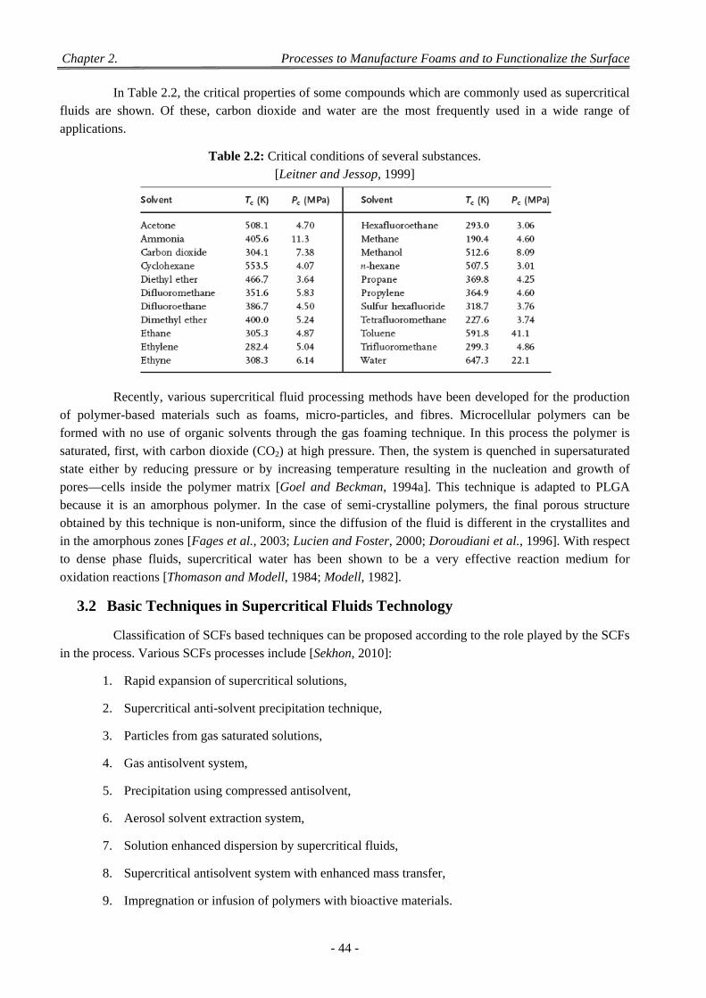
Chapter 2. Processes to Manufacture Foams and to Functionalize the Surface
- 44 -
In Table 2.2, the critical properties of some compounds which are commonly used as supercritical fluids are shown. Of these, carbon dioxide and water are the most frequently used in a wide range of
applications.
Table 2.2: Critical conditions of several substances. [Leitner and Jessop, 1999]
Recently, various supercritical fluid processing methods have been developed for the production of polymer-based materials such as foams, micro-particles, and fibres. Microcellular polymers can be formed with no use of organic solvents through the gas foaming technique. In this process the polymer is saturated, first, with carbon dioxide (CO2) at high pressure. Then, the system is quenched in supersaturated state either by reducing pressure or by increasing temperature resulting in the nucleation and growth of pores—cells inside the polymer matrix [Goel and Beckman, 1994a]. This technique is adapted to PLGA because it is an amorphous polymer. In the case of semi-crystalline polymers, the final porous structure obtained by this technique is non-uniform, since the diffusion of the fluid is different in the crystallites and in the amorphous zones [Fages et al., 2003; Lucien and Foster, 2000; Doroudiani et al., 1996]. With respect to dense phase fluids, supercritical water has been shown to be a very effective reaction medium for
oxidation reactions [Thomason and Modell, 1984; Modell, 1982].
3.2 Basic Techniques in Supercritical Fluids Technology
Classification of SCFs based techniques can be proposed according to the role played by the SCFs
in the process. Various SCFs processes include [Sekhon, 2010]:
1. Rapid expansion of supercritical solutions,
2. Supercritical anti-solvent precipitation technique,
3. Particles from gas saturated solutions,
4. Gas antisolvent system,
5. Precipitation using compressed antisolvent,
6. Aerosol solvent extraction system,
7. Solution enhanced dispersion by supercritical fluids,
8. Supercritical antisolvent system with enhanced mass transfer,
9. Impregnation or infusion of polymers with bioactive materials.
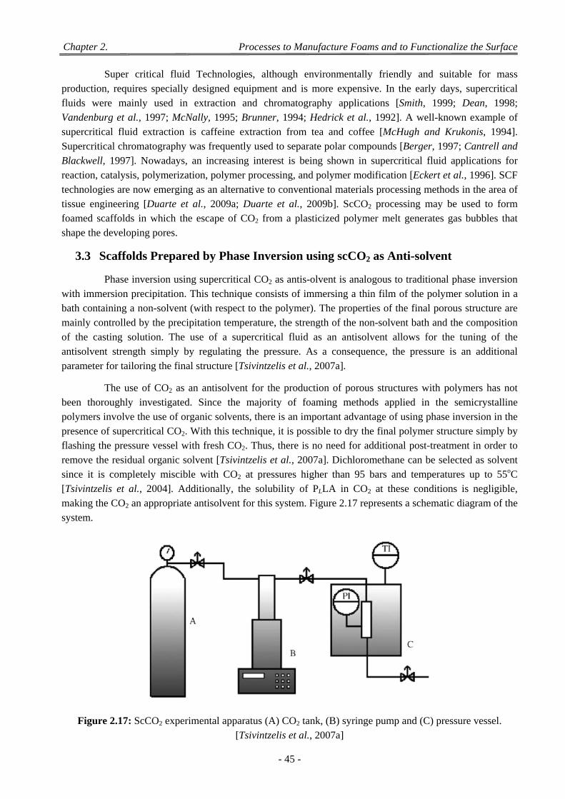
Chapter 2. Processes to Manufacture Foams and to Functionalize the Surface
- 45 -
Super critical fluid Technologies, although environmentally friendly and suitable for mass production, requires specially designed equipment and is more expensive. In the early days, supercritical fluids were mainly used in extraction and chromatography applications [Smith, 1999; Dean, 1998; Vandenburg et al., 1997; McNally, 1995; Brunner, 1994; Hedrick et al., 1992]. A well-known example of supercritical fluid extraction is caffeine extraction from tea and coffee [McHugh and Krukonis, 1994]. Supercritical chromatography was frequently used to separate polar compounds [Berger, 1997; Cantrell and Blackwell, 1997]. Nowadays, an increasing interest is being shown in supercritical fluid applications for reaction, catalysis, polymerization, polymer processing, and polymer modification [Eckert et al., 1996]. SCF technologies are now emerging as an alternative to conventional materials processing methods in the area of tissue engineering [Duarte et al., 2009a; Duarte et al., 2009b]. ScCO2 processing may be used to form foamed scaffolds in which the escape of CO2 from a plasticized polymer melt generates gas bubbles that shape the developing pores.
3.3 Scaffolds Prepared by Phase Inversion using scCO2 as Anti-solvent
Phase inversion using supercritical CO2 as antis-olvent is analogous to traditional phase inversion with immersion precipitation. This technique consists of immersing a thin film of the polymer solution in a bath containing a non-solvent (with respect to the polymer). The properties of the final porous structure are mainly controlled by the precipitation temperature, the strength of the non-solvent bath and the composition of the casting solution. The use of a supercritical fluid as an antisolvent allows for the tuning of the antisolvent strength simply by regulating the pressure. As a consequence, the pressure is an additional
parameter for tailoring the final structure [Tsivintzelis et al., 2007a].
The use of CO2 as an antisolvent for the production of porous structures with polymers has not been thoroughly investigated. Since the majority of foaming methods applied in the semicrystalline polymers involve the use of organic solvents, there is an important advantage of using phase inversion in the presence of supercritical CO2. With this technique, it is possible to dry the final polymer structure simply by flashing the pressure vessel with fresh CO2. Thus, there is no need for additional post-treatment in order to remove the residual organic solvent [Tsivintzelis et al., 2007a]. Dichloromethane can be selected as solvent since it is completely miscible with CO2 at pressures higher than 95 bars and temperatures up to 55oC [Tsivintzelis et al., 2004]. Additionally, the solubility of PLLA in CO2 at these conditions is negligible, making the CO2 an appropriate antisolvent for this system. Figure 2.17 represents a schematic diagram of the
system.
Figure 2.17: ScCO2 experimental apparatus (A) CO2 tank, (B) syringe pump and (C) pressure vessel. [Tsivintzelis et al., 2007a]
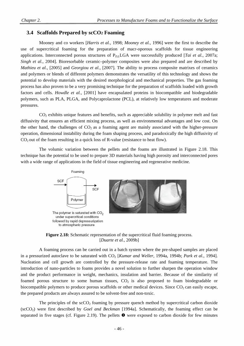
Chapter 2. Processes to Manufacture Foams and to Functionalize the Surface
- 46 -
3.4 Scaffolds Prepared by scCO2 Foaming
Mooney and co workers [Harris et al., 1998; Mooney et al., 1996] were the first to describe the use of supercritical foaming for the preparation of macr-oporous scaffolds for tissue engineering applications. Interconnected porous structures of PD,LLGA were successfully produced [Tai et al., 2007a; Singh et al., 2004]. Bioresorbable ceramic–polymer composites were also prepared and are described by Mathieu et al., [2005] and Georgiou et al., [2007]. The ability to process composite matrixes of ceramics and polymers or blends of different polymers demonstrates the versatility of this technology and shows the potential to develop materials with the desired morphological and mechanical properties. The gas foaming process has also proven to be a very promising technique for the preparation of scaffolds loaded with growth factors and cells. Howdle et al., [2001] have encapsulated proteins in biocompatible and biodegradable polymers, such as PLA, PLGA, and Polycaprolactone (PCL), at relatively low temperatures and moderate
pressures.
CO2 exhibits unique features and benefits, such as appreciable solubility in polymer melt and fast diffusivity that ensures an efficient mixing process, as well as environmental advantages and low cost. On the other hand, the challenges of CO2 as a foaming agent are mainly associated with the higher-pressure operation, dimensional instability during the foam shaping process, and paradoxically the high diffusivity of
CO2 out of the foam resulting in a quick loss of R-value (resistance to heat flow).
The volumic variation between the pellets and the foams are illustrated in Figure 2.18. This technique has the potential to be used to prepare 3D materials having high porosity and interconnected pores
with a wide range of applications in the field of tissue engineering and regenerative medicine.
Figure 2.18: Schematic representation of the supercritical fluid foaming process. [Duarte et al., 2009b]
A foaming process can be carried out in a batch system where the pre-shaped samples are placed in a pressurized autoclave to be saturated with CO2 [Kumar and Weller, 1994a, 1994b; Park et al., 1994]. Nucleation and cell growth are controlled by the pressure-release rate and foaming temperature. The introduction of nano-particles to foams provides a novel solution to further sharpen the operation window and the product performance in weight, mechanics, insulation and barrier. Because of the similarity of foamed porous structure to some human tissues, CO2 is also proposed to foam biodegradable or biocompatible polymers to produce porous scaffolds or other medical devices. Since CO2 can easily escape,
the prepared products are always assured to be solvent-free and non-toxic.
The principles of the scCO2 foaming by pressure quench method by supercritical carbon dioxide (scCO2) were first described by Goel and Beckman [1994a]. Schematically, the foaming effect can be separated in five stages (cf. Figure 2.19). The pellets were exposed to carbon dioxide for few minutes
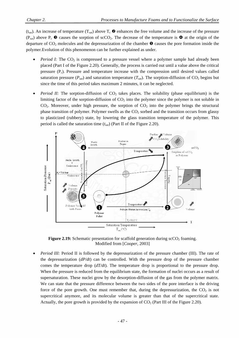
Chapter 2. Processes to Manufacture Foams and to Functionalize the Surface
- 47 -
(tsat). An increase of temperature (Tsat) above Tc enhances the free volume and the increase of the pressure (Psat) above Pc causes the sorption of scCO2. The decrease of the temperature is at the origin of the departure of CO2 molecules and the depressurization of the chamber causes the pore formation inside the
polymer.Evolution of this phenomenon can be further explained as under.
Period I: The CO2 is compressed to a pressure vessel where a polymer sample had already been placed (Part I of the Figure 2.20). Generally, the process is carried out until a value above the critical pressure (Pc). Pressure and temperature increase with the compression until desired values called saturation pressure (Psat) and saturation temperature (Tsat). The sorption-diffusion of CO2 begins but
since the time of this period takes maximum 2 minutes, it can be neglected.
Period II: The sorption-diffusion of CO2 takes places. The solubility (phase equilibrium) is the limiting factor of the sorption-diffusion of CO2 into the polymer since the polymer is not soluble in CO2. Moreover, under high pressure, the sorption of CO2 into the polymer brings the structural phase transition of polymer. Polymer swells as the CO2 sorbed and the transition occurs from glassy to plasticized (rubbery) state, by lowering the glass transition temperature of the polymer. This
period is called the saturation time (tsat) (Part II of the Figure 2.20).
Figure 2.19: Schematic presentation for scaffold generation during scCO2 foaming. Modified from [Cooper, 2003]
Period III: Period II is followed by the depressurization of the pressure chamber (III). The rate of the depressurization (dP/dt) can be controlled. With the pressure drop of the pressure chamber comes the temperature drop (dT/dt). The temperature drop is proportional to the pressure drop. When the pressure is reduced from the equilibrium state, the formation of nuclei occurs as a result of supersaturation. These nuclei grow by the desorption-diffusion of the gas from the polymer matrix. We can state that the pressure difference between the two sides of the pore interface is the driving force of the pore growth. One must remember that, during the depressurization, the CO2 is not supercritical anymore, and its molecular volume is greater than that of the supercritical state.
Actually, the pore growth is provided by the expansion of CO2 (Part III of the Figure 2.20).
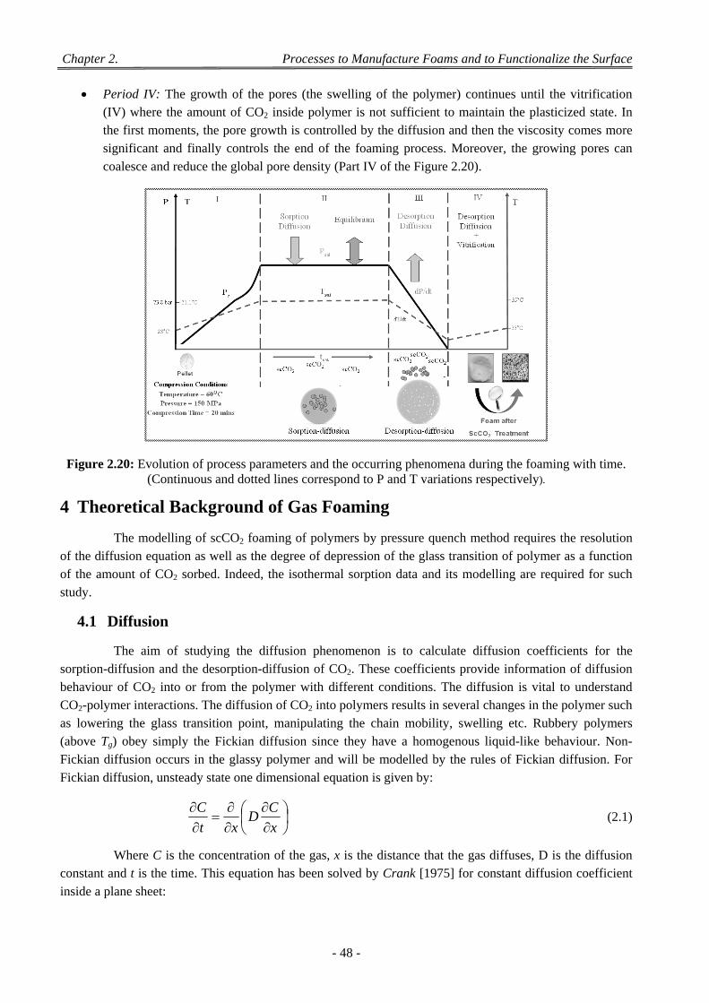
Chapter 2. Processes to Manufacture Foams and to Functionalize the Surface
- 48 -
Period IV: The growth of the pores (the swelling of the polymer) continues until the vitrification (IV) where the amount of CO2 inside polymer is not sufficient to maintain the plasticized state. In the first moments, the pore growth is controlled by the diffusion and then the viscosity comes more significant and finally controls the end of the foaming process. Moreover, the growing pores can
coalesce and reduce the global pore density (Part IV of the Figure 2.20).
Figure 2.20: Evolution of process parameters and the occurring phenomena during the foaming with time. (Continuous and dotted lines correspond to P and T variations respectively).
4 Theoretical Background of Gas Foaming
The modelling of scCO2 foaming of polymers by pressure quench method requires the resolution of the diffusion equation as well as the degree of depression of the glass transition of polymer as a function of the amount of CO2 sorbed. Indeed, the isothermal sorption data and its modelling are required for such
study.
4.1 Diffusion
The aim of studying the diffusion phenomenon is to calculate diffusion coefficients for the sorption-diffusion and the desorption-diffusion of CO2. These coefficients provide information of diffusion behaviour of CO2 into or from the polymer with different conditions. The diffusion is vital to understand CO2-polymer interactions. The diffusion of CO2 into polymers results in several changes in the polymer such as lowering the glass transition point, manipulating the chain mobility, swelling etc. Rubbery polymers (above Tg) obey simply the Fickian diffusion since they have a homogenous liquid-like behaviour. Non-Fickian diffusion occurs in the glassy polymer and will be modelled by the rules of Fickian diffusion. For
Fickian diffusion, unsteady state one dimensional equation is given by:
x
CD
xt
C (2.1)
Where C is the concentration of the gas, x is the distance that the gas diffuses, D is the diffusion constant and t is the time. This equation has been solved by Crank [1975] for constant diffusion coefficient
inside a plane sheet:
Chapter 2. Processes to Manufacture Foams and to Functionalize the Surface
- 49 -
2
22
022 4
)12(exp
)12(
81
a
tnD
nM
M
n
t
(2.2)
where a is the semi-thickness of the polymer pellet, Mt denotes the total amount of diffusing substance which has entered the polymer during time t, and M∞ the corresponding quantity after infinite time. On the other hand, in the case of the desorption-diffusion, M∞ denotes the amount of CO2 at zero time, Mt, the
quantity of CO2 which remains in the polymer at time t and n is gas molecules per cm3.
The reduced version of Equation (2.2) for short times is also given by [Crank, 1975].
1
2
12
1
2 )()1(22
n
nt
Dt
naierfc
a
Dt
M
M (2.3)
Literature and experimental work revealed that, during the sorption and desorption of CO2 into the polymer, the diffusion coefficient is not constant. It depends on the concentration of CO2 sorbed by polymer. One can say that the more CO2 absorbed, the more CO2 can diffuse easily into or from the polymer. The dependency of the diffusion coefficient on the concentration is due to the several effects caused by the sorption of the CO2 into the polymer matrix such as manipulation of the polymer matrix, swelling (decreasing the bulk polymer density), lowering the glass transition point, lowering the interfacial tension and the viscosity of the polymer. Also, by activated state theory the diffusion coefficient is also temperature
dependent and it increases with the increasing temperature [Koros and Madden, 2004].
As proposed by Crank, the average diffusivity of CO2 in polymers can be measured in a desorption experiment. For early stages of diffusion (sorption or desorption), the amount of gas remaining in a plane sample at any time is related to the diffusion coefficient. This procedure has been applied to analyze the sorption of CO2 into the polymers [Kumar and Weller, 1994b; Berens and Huvard, 1989b], and it can be
used when the sorption curve is plotted against 2/ lt , where l is the thickness of sample, if it is
approximately linear as far as Mt/M∞ = 0.5.
The Sanchez-Lacombe’s equation of state (SL-EOS) has been used to predict the behaviours of polymer-gas mixtures [Sanchez and Lacombe, 1976]. SL-EOS is a well defined statistical mechanical model which is not a physical model of sorption of a gas into a polymer but an equation of state which defines the capacity of sorption as well as the swelling of the polymer. The SL-EOS is known as a lattice-gas model since the P-V-T properties of a pure component are calculated assuming that the component is broken into parts or “mers” that are placed into a lattice and are allowed to interact with a mean-field-type intermolecular potential. To obtain the correct system density, an appropriate number of holes is also put into specific lattice sites, hence the name lattice-gas model [McHugh and Krukonis, 1994]. We have to underline that this equation can be used for rubbery and glassy states of the amorphous or liquid-like
polymers. In its basic form, the SL-EOS is given by:
0)1
1()1ln(2
RRRRR r
TP (2.4)
where TR, PR, ρR are reduced temperature, pressure and density respectively and r represents the number of
lattice sites occupied by one molecule.
The reduced parameters can be calculated by:
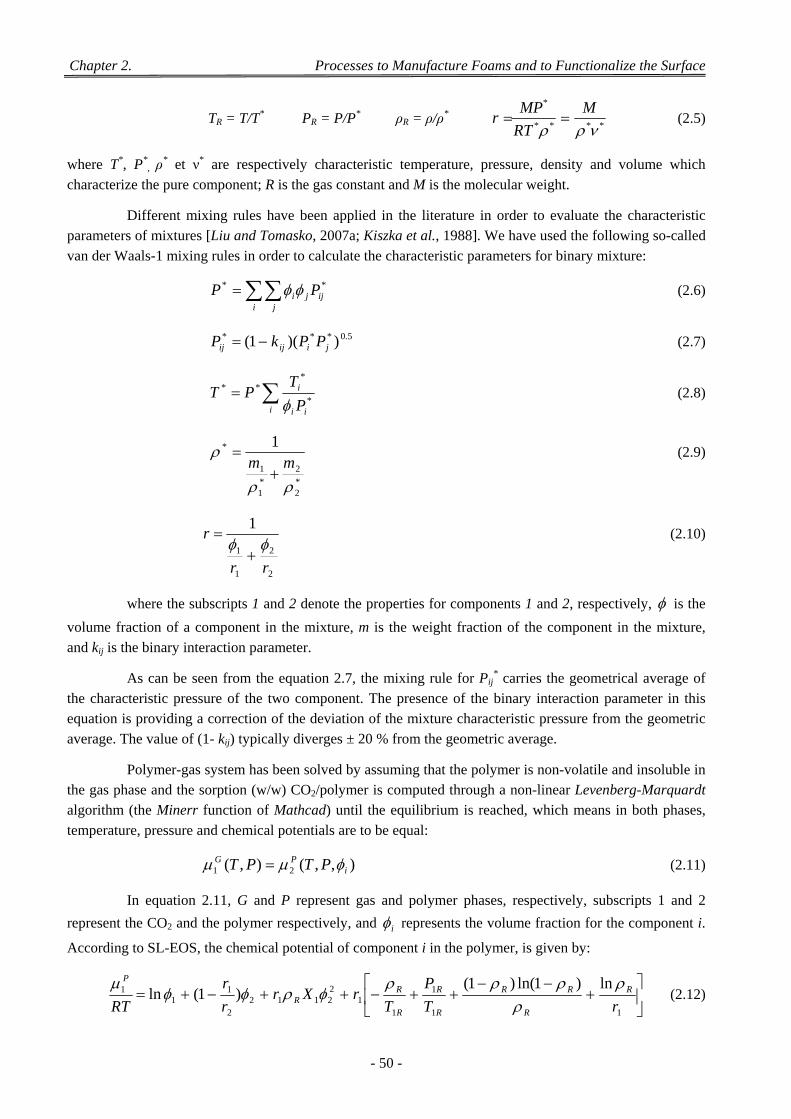
Chapter 2. Processes to Manufacture Foams and to Functionalize the Surface
- 50 -
TR = T/T* PR = P/P* ρR = ρ/ρ* ****
*
M
RT
MPr (2.5)
where T*, P*, ρ
* et ν* are respectively characteristic temperature, pressure, density and volume which
characterize the pure component; R is the gas constant and M is the molecular weight.
Different mixing rules have been applied in the literature in order to evaluate the characteristic parameters of mixtures [Liu and Tomasko, 2007a; Kiszka et al., 1988]. We have used the following so-called
van der Waals-1 mixing rules in order to calculate the characteristic parameters for binary mixture:
i j
ijji PP ** (2.6)
5.0*** ))(1( jiijij PPkP (2.7)
i ii
i
P
TPT
*
***
(2.8)
*2
2
*1
1
* 1
mm
(2.9)
2
2
1
1
1
rr
r
(2.10)
where the subscripts 1 and 2 denote the properties for components 1 and 2, respectively, is the
volume fraction of a component in the mixture, m is the weight fraction of the component in the mixture,
and kij is the binary interaction parameter.
As can be seen from the equation 2.7, the mixing rule for Pij* carries the geometrical average of
the characteristic pressure of the two component. The presence of the binary interaction parameter in this equation is providing a correction of the deviation of the mixture characteristic pressure from the geometric
average. The value of (1- kij) typically diverges ± 20 % from the geometric average.
Polymer-gas system has been solved by assuming that the polymer is non-volatile and insoluble in the gas phase and the sorption (w/w) CO2/polymer is computed through a non-linear Levenberg-Marquardt algorithm (the Minerr function of Mathcad) until the equilibrium is reached, which means in both phases,
temperature, pressure and chemical potentials are to be equal:
),,(),( 21 iPG PTPT (2.11)
In equation 2.11, G and P represent gas and polymer phases, respectively, subscripts 1 and 2
represent the CO2 and the polymer respectively, and i represents the volume fraction for the component i.
According to SL-EOS, the chemical potential of component i in the polymer, is given by:
11
1
11
22112
2
11
1 ln)1ln()1()1(ln
rT
P
TrXr
r
r
RTR
R
RR
R
R
R
RR
P
(2.12)
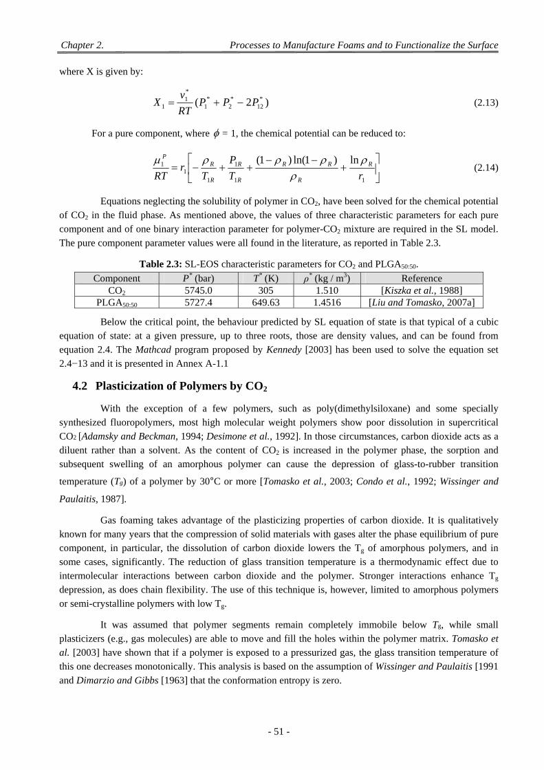
Chapter 2. Processes to Manufacture Foams and to Functionalize the Surface
- 51 -
where X is given by:
)2( *12
*2
*1
*1
1 PPPRT
vX (2.13)
For a pure component, where = 1, the chemical potential can be reduced to:
11
1
11
1 ln)1ln()1(
rT
P
Tr
RTR
R
RR
R
R
R
RP
(2.14)
Equations neglecting the solubility of polymer in CO2, have been solved for the chemical potential of CO2 in the fluid phase. As mentioned above, the values of three characteristic parameters for each pure component and of one binary interaction parameter for polymer-CO2 mixture are required in the SL model.
The pure component parameter values were all found in the literature, as reported in Table 2.3.
Table 2.3: SL-EOS characteristic parameters for CO2 and PLGA50:50.
Component P* (bar) T* (K) ρ* (kg / m3) Reference CO2 5745.0 305 1.510 [Kiszka et al., 1988]
PLGA50:50 5727.4 649.63 1.4516 [Liu and Tomasko, 2007a]
Below the critical point, the behaviour predicted by SL equation of state is that typical of a cubic equation of state: at a given pressure, up to three roots, those are density values, and can be found from equation 2.4. The Mathcad program proposed by Kennedy [2003] has been used to solve the equation set
2.4−13 and it is presented in Annex A-1.1
4.2 Plasticization of Polymers by CO2
With the exception of a few polymers, such as poly(dimethylsiloxane) and some specially synthesized fluoropolymers, most high molecular weight polymers show poor dissolution in supercritical CO2 [Adamsky and Beckman, 1994; Desimone et al., 1992]. In those circumstances, carbon dioxide acts as a diluent rather than a solvent. As the content of CO2 is increased in the polymer phase, the sorption and subsequent swelling of an amorphous polymer can cause the depression of glass-to-rubber transition
temperature (Tg) of a polymer by 30°C or more [Tomasko et al., 2003; Condo et al., 1992; Wissinger and
Paulaitis, 1987].
Gas foaming takes advantage of the plasticizing properties of carbon dioxide. It is qualitatively known for many years that the compression of solid materials with gases alter the phase equilibrium of pure component, in particular, the dissolution of carbon dioxide lowers the Tg of amorphous polymers, and in some cases, significantly. The reduction of glass transition temperature is a thermodynamic effect due to intermolecular interactions between carbon dioxide and the polymer. Stronger interactions enhance Tg depression, as does chain flexibility. The use of this technique is, however, limited to amorphous polymers
or semi-crystalline polymers with low Tg.
It was assumed that polymer segments remain completely immobile below Tg, while small plasticizers (e.g., gas molecules) are able to move and fill the holes within the polymer matrix. Tomasko et al. [2003] have shown that if a polymer is exposed to a pressurized gas, the glass transition temperature of this one decreases monotonically. This analysis is based on the assumption of Wissinger and Paulaitis [1991
and Dimarzio and Gibbs [1963] that the conformation entropy is zero.
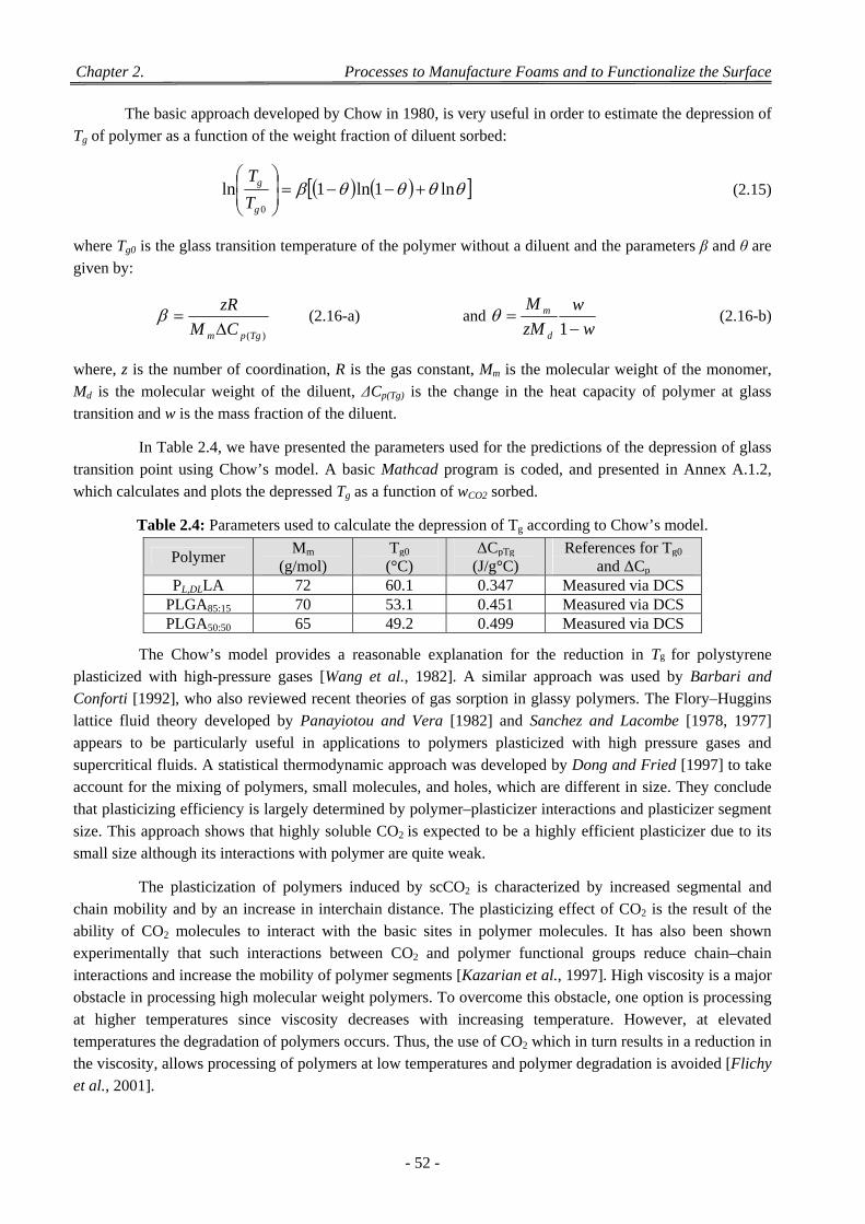
Chapter 2. Processes to Manufacture Foams and to Functionalize the Surface
- 52 -
The basic approach developed by Chow in 1980, is very useful in order to estimate the depression of
Tg of polymer as a function of the weight fraction of diluent sorbed:
ln1ln1ln0
g
g
T
T (2.15)
where Tg0 is the glass transition temperature of the polymer without a diluent and the parameters β and θ are
given by:
)(Tgpm CM
zR
(2.16-a) and
w
w
zM
M
d
m
1 (2.16-b)
where, z is the number of coordination, R is the gas constant, Mm is the molecular weight of the monomer, Md is the molecular weight of the diluent, ΔCp(Tg) is the change in the heat capacity of polymer at glass
transition and w is the mass fraction of the diluent.
In Table 2.4, we have presented the parameters used for the predictions of the depression of glass transition point using Chow’s model. A basic Mathcad program is coded, and presented in Annex A.1.2,
which calculates and plots the depressed Tg as a function of wCO2 sorbed.
Table 2.4: Parameters used to calculate the depression of Tg according to Chow’s model.
Polymer Mm
(g/mol) Tg0 (°C)
ΔCpTg (J/g°C)
References for Tg0 and ΔCp
PL,DLLA 72 60.1 0.347 Measured via DCS PLGA85:15 70 53.1 0.451 Measured via DCS PLGA50:50 65 49.2 0.499 Measured via DCS
The Chow’s model provides a reasonable explanation for the reduction in Tg for polystyrene plasticized with high-pressure gases [Wang et al., 1982]. A similar approach was used by Barbari and Conforti [1992], who also reviewed recent theories of gas sorption in glassy polymers. The Flory–Huggins lattice fluid theory developed by Panayiotou and Vera [1982] and Sanchez and Lacombe [1978, 1977] appears to be particularly useful in applications to polymers plasticized with high pressure gases and supercritical fluids. A statistical thermodynamic approach was developed by Dong and Fried [1997] to take account for the mixing of polymers, small molecules, and holes, which are different in size. They conclude that plasticizing efficiency is largely determined by polymer–plasticizer interactions and plasticizer segment size. This approach shows that highly soluble CO2 is expected to be a highly efficient plasticizer due to its
small size although its interactions with polymer are quite weak.
The plasticization of polymers induced by scCO2 is characterized by increased segmental and chain mobility and by an increase in interchain distance. The plasticizing effect of CO2 is the result of the ability of CO2 molecules to interact with the basic sites in polymer molecules. It has also been shown experimentally that such interactions between CO2 and polymer functional groups reduce chain–chain interactions and increase the mobility of polymer segments [Kazarian et al., 1997]. High viscosity is a major obstacle in processing high molecular weight polymers. To overcome this obstacle, one option is processing at higher temperatures since viscosity decreases with increasing temperature. However, at elevated temperatures the degradation of polymers occurs. Thus, the use of CO2 which in turn results in a reduction in the viscosity, allows processing of polymers at low temperatures and polymer degradation is avoided [Flichy
et al., 2001].
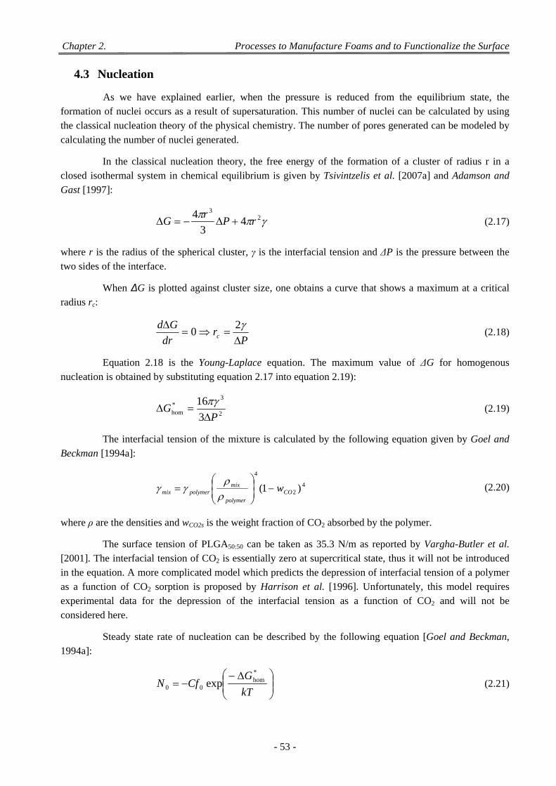
Chapter 2. Processes to Manufacture Foams and to Functionalize the Surface
- 53 -
4.3 Nucleation
As we have explained earlier, when the pressure is reduced from the equilibrium state, the formation of nuclei occurs as a result of supersaturation. This number of nuclei can be calculated by using the classical nucleation theory of the physical chemistry. The number of pores generated can be modeled by
calculating the number of nuclei generated.
In the classical nucleation theory, the free energy of the formation of a cluster of radius r in a closed isothermal system in chemical equilibrium is given by Tsivintzelis et al. [2007a] and Adamson and
Gast [1997]:
23
43
4rP
rG (2.17)
where r is the radius of the spherical cluster, γ is the interfacial tension and ΔP is the pressure between the
two sides of the interface.
When ΔG is plotted against cluster size, one obtains a curve that shows a maximum at a critical radius rc:
Pr
dr
Gdc
20 (2.18)
Equation 2.18 is the Young-Laplace equation. The maximum value of ΔG for homogenous
nucleation is obtained by substituting equation 2.17 into equation 2.19):
2
3*hom 3
16
PG
(2.19)
The interfacial tension of the mixture is calculated by the following equation given by Goel and
Beckman [1994a]:
42
4
)1( COpolymer
mixpolymermix w
(2.20)
where ρ are the densities and wCO2s is the weight fraction of CO2 absorbed by the polymer.
The surface tension of PLGA50:50 can be taken as 35.3 N/m as reported by Vargha-Butler et al. [2001]. The interfacial tension of CO2 is essentially zero at supercritical state, thus it will not be introduced in the equation. A more complicated model which predicts the depression of interfacial tension of a polymer as a function of CO2 sorption is proposed by Harrison et al. [1996]. Unfortunately, this model requires experimental data for the depression of the interfacial tension as a function of CO2 and will not be
considered here.
Steady state rate of nucleation can be described by the following equation [Goel and Beckman,
1994a]:
kT
GCfN
*hom
00 exp (2.21)
Chapter 2. Processes to Manufacture Foams and to Functionalize the Surface
- 54 -
where C is the concentration of the dissolved fluid inside the polymer matrix (number of molecules per volume), k is the Boltzmann constant, T is the temperature and f0 the frequency factor for the gas molecules,
which describes the rate at which nuclei with critical radius are transformed into stable bubbles.
Frequency factor f0 can be expressed as a function of the critical radius [Goel and Beckman, 1994a]:
20 4 cimp rZRf (2.22)
where Z is the Zeldovich factor and Rimp is the impingement rate of the gas molecules per unit area. ZRimp
can be used as a one time fitter parameter within the calculations.
Since foaming is an unsteady state process, we have to take into consideration time as a variable and integrate the nucleation rate in order to calculate total number of nuclei generated within the nucleation
time:
vitrP
satP
vitrt
total dtdP
dPNdtNN
,
,
0
,
0
0 (2.23)
where sat and vitr denotes the saturation and vitrification respectively.
It is in our knowledge that the foaming of polymers occurs while the CO2 is desorbs. Hence, one can say that the dissolved amount of fluid in the polymer matrix is not constant within the foaming time and it decreases. Also, while foaming occurs, polymer swells as the CO2 changes its state from supercritical to gas (the volume of CO2 increases). So, one can say that in the presence of these two effects the concentration of CO2 in the matrix decreases. This concentration dependency must be placed in the nucleation rate equation and nucleation rate must be integrated with time. One can model the decrease of mass within the foaming time by using equation 2.3 and fitting it to the desorption data. The change within the volume can be expressed with a linear relationship between initial and final volumes. One can assume that there is no volume change after vitrification. The variation of CO2 concentration is not considered in the existing
model.
4.4 Distribution of Pores
Scaffolds must meet certain fundamental characteristics such as high porosity, appropriate pore size, biocompatibility, biodegradability and proper degradation rate [Ma and Choi, 2001]. Scaffolds for tissues require specific properties such as an interconnected porosity higher than 75% to provide a high void volume for nutrient diffusion [Temenoff et al., 2000]. Furthermore an optimal pore size necessary to promote cell adhesion must be in the range of 100−300 μm [Boyan et al., 1996]. Finally, mechanical properties should approximate those of native cartilage bone, in order to support body load and avoid excessive micro-
motions at the scaffold/bone interface [Büchler et al., 2003; Temenoff et al., 2000].
Ideally a scaffold should possess the following characteristics containing the desired biologic
response [Hutmacher, 2001]:
three-dimensional and highly porous with an interconnected pore network for cell/tissue growth and flow transport of nutrients and metabolic waste,
biodegradable or bioresorbable with a controllable degradation and resorption rate to match cell/tissue growth in vitro and/or in vivo,
suitable surface chemistry for cell attachment, proliferation and differentiation,
Chapter 2. Processes to Manufacture Foams and to Functionalize the Surface
- 55 -
mechanical properties matching those of tissues at the site of implantation,
easily processable to form a variety of shapes and sizes.
In batch foaming, a polymer in disc or powder form is subjected to supercritical CO2 flow without mixing. After venting the CO2 by depressurization, thermodynamic instability causes supersaturation of the CO2 dissolved in the polymer matrix and hence, nucleation of cells occurs. The growth of the cells continues until the polymer vitrifies. The saturation pressure, the saturation temperature and the depressurization rate are the critical parameters in determining the number of cells and the cell size distribution. To predict the pore size of foams created, in the literature, there is several numbers of influential studies on diffusion-induced pore growth. These models consider the polymer as a Maxwell fluid and solve systems of partial
differential equations by numerical methods [Goel and Beckman, 1995; Arefmanesh and Advani, 1991].
The cell number density increased and the cell size decreased with increasing pressure and decreasing temperature. A high degree of super-saturation of dissolved CO2 at high pressure and low temperature are responsible for such results. Classical homogeneous nucleation theory is generally used to calculate the nucleation rate in foaming with supercritical CO2. The energy barrier for nucleation in the theory can be calculated as a function of the interfacial tension of the binary mixture and the magnitude of the pressure drop. The theory suggests that the energy barrier and the interfacial tension decrease as the pressure drop increases. Consequently, the nucleation rate increases and a large number of small cells is obtained. In fact, both the pressure drop rate and the magnitude of the pressure drop determine the cell density and cell size in microcellular foaming. The higher the pressure drop rate, the greater the nucleation rate due to the high supersaturation rate. This allows only a short time for existing cells to grow and, consequently, is in favour of formation of small cells. Classical nucleation theory fails to incorporate the effect of the pressure drop rate. Moreover, a noteworthy study on CO2-assisted microcellular foaming of PLGA is reported by Sparacio and Beckman [1998], in which a minimum in cell size with increasing pressure was found instead of the levelling off according to theory. A plausible explanation is low resistance to cell growth due to a large decrease in the melting point of the polymer and very low interfacial tension at
high pressure.
Detailed studies of the glassy polymer – CO2 system by Wessling et al. [1994] suggest that the nucleation mechanism underlying the foaming process is heterogeneous in nature. The significant advance made by [Wessling et al., 1994] was that they were able to detect and explained the appearance not only of the porous structure in the polymer film after saturation with CO2 but also of a dense layer next to the porous layer. They provided a physical explanation and a mathematical model to predict the thickness of this dense layer. The studies of McCarthy and coworkers [Stafford et al., 1999; Arora et al., 1998a] on the effect of the residual oligomer in polystyrene on its foaming with scCO2 have shown that its presence affects the cell size in these foams. This work also questioned the ability of classical nucleation theory to explain the foaming mechanism in these systems, and the authors suggest a spinodal mechanism as an alternative route of cell formation [Stafford et al., 1999]. Foaming of polypropylene has also been studied extensively by Park and Cheung [1997], with the most recent report by Liang and Wang [1999], who highlighted the effect of temperature drop during depressurization of the polymer in equilibrium with high-pressure CO2. Handa and Zhang [2000] used the existence of a rubbery state in the PMMA at low temperatures to generate foams by
saturating the polymer with CO2 at 24C to 90C. They demonstrated that the solubility of CO2 in the
polymer plays an important role in controlling cell density and cell size. Thus, the solubility of CO2 at 34
bars and temperature of – 0.2C is 22.5% (w/w), while at the same pressure but at 24C, the solubility is just
7.9% (w/w).
Chapter 2. Processes to Manufacture Foams and to Functionalize the Surface
- 56 -
Another approach to create microcellular materials was demonstrated by Shi et al. [1999]. First, they synthesized a number of chemicals soluble in scCO2 or liquid CO2. These chemicals comprise a number of “monomers” containing one or two urea groups and fluorinated “tail” groups that enhance solubility of these compounds in CO2. When these compounds were dissolved in CO2, their self-association led to the formation of gels. The removal of CO2 via depressurization resulted in the formation of foams with cells
with an average diameter of less than 1 m. Shi et al. [1999] reported that the bulk density reduction of these
foams was 97% compared to the parent materials. Sheridan et al. [2000] studied the effects of several processing parameters (such as polymer composition, molecular mass, and gas type) on preparing three-dimensional porous matrices from copolymers of lactide and glycolide and demonstrated that crystalline polymers did not produce foamed materials via this approach, while gas treatment of amorphous copolymers produced matrices with porosity up to 95%. This work also demonstrated that only CO2 among the other gases used (e.g., N2 and He) created highly porous polymer structures in these copolymers [Sheridan et al., 2000] and explained this by the possible interactions between CO2 and carbonyl groups in PLGA [Kazarian
et al., 1996a].
5 Manufacturing of the Composite Biomaterials
5.1 Fundements of Co-grinding Process
5.1.1 Mechanism of Size Reduction
The properties of a material may be considerably influenced by the particle size and, for example, the chemical reactivity of fine particles is greater than that of coarse particles. In addition, far more intimate mixing of solids can be achieved if the particle size is small [Richardson et al., 2002]. Practically every solid
material undergoes size reduction at some point in its processing cycle.
Also reduction in size causes [Richardson et al., 2002]:
Both an increase in area and a reduction in the distance.
Separation of constituents, especially where one is dispersed in small isolated pockets.
Properties of a material may be considerably influenced by the particle size.
Chemical reactivity of fine particles is greater than that of coarse particles.
In addition, far more intimate mixing of solids can be achieved if the particle size is small.
The mechanism of the process of fragmentation is extremely complex. If a single lump of material is subjected to a sudden impact, it will generally break so as to yield a few relatively large particles and a number of fine particles, with relatively few particles of intermediate size. If the energy in the blow is increased, the larger particles will be of a rather smaller size and more numerous and, whereas the number of fine particles will be appreciably increased, their size will not be much altered. It therefore appears that the
size of the fine particles is closely connected with the internal structure of the material.
During the course of the size reduction processes, much energy is expended in causing plastic deformation and this energy may be regarded as a waste as it does not result in fracture. Only part of it is retained in the system as a result of elastic recovery. It is not possible, however, to achieve the stress levels necessary for fracture to occur without first passing through the condition of plastic deformation and, in this sense, this must be regarded as a necessary state which must be achieved before fracture can possibly occur
[Richardson et al., 2002].
Chapter 2. Processes to Manufacture Foams and to Functionalize the Surface
- 57 -
The method of application of the force to the particles may affect the breakage pattern. Four basic patterns may be identified, though it is sometimes difficult to identify the dominant mode in any given
machine [Richardson et al., 2002].
Impact: particle concussion by a single rigid force.
Compression: particle disintegration by two rigid forces.
Shear: produced by a fluid or by particle–particle interaction.
Attrition: arising from particles scraping against one another or against a rigid surface.
5.1.2 Fragmentation Mechanisms
The reduction of the material in small fragments or in powder is obtained by the operation of grinding. The mechanism of grinding can be explained by the theory of the fracture mechanics and finally
the fracture of particles subjected to the mechanical forces.
The resulting stress field generally depends on, as reported by Zapata-Massot [2004]:
Intrinsic parameters to the materials: they determine its behaviour at the time of the deformation. The field of constraints determines the dimension, the form of the fragments and the new created
surfaces.
The required energy to break the material: the necessary energy to the rupture is additional energy for the propagation of a fissure is energy consumer. It is proportional to the section of the grain
while the energy stored is proportional to the volume.
Rate of deformation: it conditions the behaviour of the material.
Reduction of the dimensions of the material: it is not limitless and necessitates most of the time of
the successive phases implying typical different of devices working mass.
The fragmentation process is a part of the size reduction process. Granular materials submitted to fine grinding may be subject to several modes of fragmentation (abrasion, chipping, cleavage, breakage) [Render, 1990]. The size evolution is not sufficient to clearly explain the grinding mechanisms. Thus other properties such as morphology have to be considered. Indeed, it is recognized that the end-use properties of a powder are influenced not only by the size but also by the shape of the particles. Qualitative SEM observations have been used to explain assumptions on phenomena appearing in the mills. However, the knowledge of particle fragmentation has been limited. Thus, a quantification of the morphology evolution during grinding is needed. Experimental studies, carried out using various materials, have shown that the size decrease occurs in steps, which suggests that the fragmentation mechanism is complex [Molina-
Boisseau et al., 2002].
5.1.3 Agglomeration Phenomena
The agglomeration phenomena occur during the co-grinding of amorphous polymer material and
powder filler.
Size enlargement is any process whereby small particles are gathered into larger, relatively
permanent masses in which the original particles can still be distinguished.
Agglomeration is the formation of aggregates through the sticking together of feed and/or recycle
material [Perry et al., 1997].
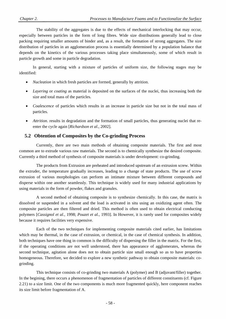
Chapter 2. Processes to Manufacture Foams and to Functionalize the Surface
- 58 -
The stability of the aggregates is due to the effects of mechanical interlocking that may occur, especially between particles in the form of long fibres. Wide size distributions generally lead to close packing requiring smaller amounts of binder and, as a result, the formation of strong aggregates. The size distribution of particles in an agglomeration process is essentially determined by a population balance that depends on the kinetics of the various processes taking place simultaneously, some of which result in
particle growth and some in particle degradation.
In general, starting with a mixture of particles of uniform size, the following stages may be
identified:
Nucleation in which fresh particles are formed, generally by attrition.
Layering or coating as material is deposited on the surfaces of the nuclei, thus increasing both the size and total mass of the particles.
Coalescence of particles which results in an increase in particle size but not in the total mass of
particles.
Attrition. results in degradation and the formation of small particles, thus generating nuclei that re-enter the cycle again [Richardson et al., 2002].
5.2 Obtention of Composites by the Co-grinding Process
Currently, there are two main methods of obtaining composite materials. The first and most common are to extrude various raw materials. The second is to chemically synthesize the desired composite.
Currently a third method of synthesis of composite materials is under development: co-grinding.
The products from Extrusion are preheated and introduced upstream of an extrusion screw. Within the extruder, the temperature gradually increases, leading to a change of state products. The use of screw extrusion of various morphologies can perform an intimate mixture between different compounds and disperse within one another seamlessly. This technique is widely used for many industrial applications by
using materials in the form of powder, flakes and granules.
A second method of obtaining composite is to synthesize chemically. In this case, the matrix is dissolved or suspended in a solvent and the load is activated in situ using an oxidizing agent often. The composite particles are then filtered and dried. This method is often used to obtain electrical conducting polymers [Cassignol et al., 1998; Pouzet et al., 1993]. In However, it is rarely used for composites widely
because it requires facilities very expensive.
Each of the two techniques for implementing composite materials cited earlier, has limitations which may be thermal, in the case of extrusion, or chemical, in the case of chemical synthesis. In addition, both techniques have one thing in common is the difficulty of dispersing the filler in the matrix. For the first, if the operating conditions are not well understood, there has appearance of agglomerates, whereas the second technique, agitation alone does not to obtain particle size small enough so as to have properties homogeneous. Therefore, we decided to explore a new synthetic pathway to obtain composite materials: co-
grinding.
This technique consists of co-grinding two materials A (polymer) and B (adjuvant/filler) together. In the begining, there occurs a phenomenon of fragmentation of particles of different constituents (cf. Figure 2.21) to a size limit. One of the two components is much more fragmented quickly, here component reaches
its size limit before fragmentation of A.
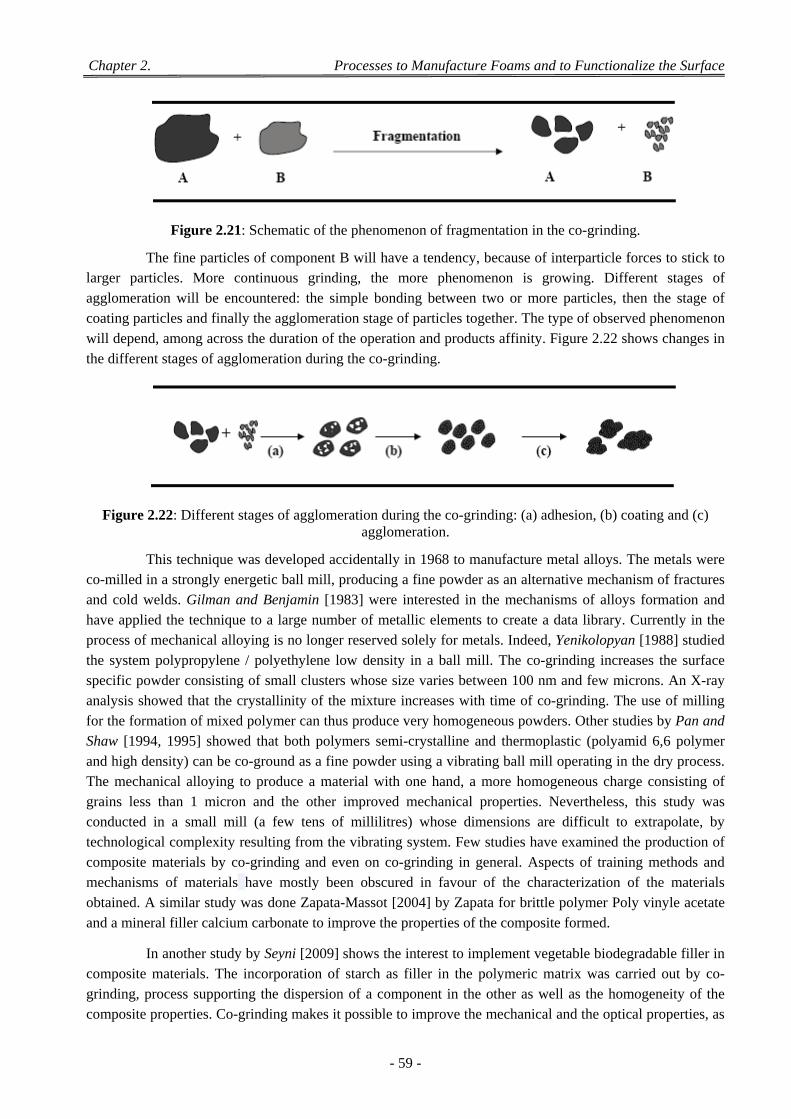
Chapter 2. Processes to Manufacture Foams and to Functionalize the Surface
- 59 -
Figure 2.21: Schematic of the phenomenon of fragmentation in the co-grinding.
The fine particles of component B will have a tendency, because of interparticle forces to stick to larger particles. More continuous grinding, the more phenomenon is growing. Different stages of agglomeration will be encountered: the simple bonding between two or more particles, then the stage of coating particles and finally the agglomeration stage of particles together. The type of observed phenomenon will depend, among across the duration of the operation and products affinity. Figure 2.22 shows changes in
the different stages of agglomeration during the co-grinding.
Figure 2.22: Different stages of agglomeration during the co-grinding: (a) adhesion, (b) coating and (c) agglomeration.
This technique was developed accidentally in 1968 to manufacture metal alloys. The metals were co-milled in a strongly energetic ball mill, producing a fine powder as an alternative mechanism of fractures and cold welds. Gilman and Benjamin [1983] were interested in the mechanisms of alloys formation and have applied the technique to a large number of metallic elements to create a data library. Currently in the process of mechanical alloying is no longer reserved solely for metals. Indeed, Yenikolopyan [1988] studied the system polypropylene / polyethylene low density in a ball mill. The co-grinding increases the surface specific powder consisting of small clusters whose size varies between 100 nm and few microns. An X-ray analysis showed that the crystallinity of the mixture increases with time of co-grinding. The use of milling for the formation of mixed polymer can thus produce very homogeneous powders. Other studies by Pan and Shaw [1994, 1995] showed that both polymers semi-crystalline and thermoplastic (polyamid 6,6 polymer and high density) can be co-ground as a fine powder using a vibrating ball mill operating in the dry process. The mechanical alloying to produce a material with one hand, a more homogeneous charge consisting of grains less than 1 micron and the other improved mechanical properties. Nevertheless, this study was conducted in a small mill (a few tens of millilitres) whose dimensions are difficult to extrapolate, by technological complexity resulting from the vibrating system. Few studies have examined the production of composite materials by co-grinding and even on co-grinding in general. Aspects of training methods and mechanisms of materials have mostly been obscured in favour of the characterization of the materials obtained. A similar study was done Zapata-Massot [2004] by Zapata for brittle polymer Poly vinyle acetate
and a mineral filler calcium carbonate to improve the properties of the composite formed.
In another study by Seyni [2009] shows the interest to implement vegetable biodegradable filler in composite materials. The incorporation of starch as filler in the polymeric matrix was carried out by co-grinding, process supporting the dispersion of a component in the other as well as the homogeneity of the composite properties. Co-grinding makes it possible to improve the mechanical and the optical properties, as
Chapter 2. Processes to Manufacture Foams and to Functionalize the Surface
- 60 -
well as the resistance to water of the material, not only from the improvement of the dispersion homogeneity
of the filler in the matrix, but also thanks to a modification of the interface quality.
6 Conclusion
Different processes for manufacturing scaffolds were discussed in detail with advantages and disadvantages. Scaffolds obtained by each technique posses typical structure and morphology and can be used as per requirement. Scaffolds for tissue engineering should encourage the growth, migration, and organization of cells, providing support while the tissue is forming the scaffolds will be replaced with host cells and a new extracellular matrix which in turn should provide functional and mechanical properties, similar to native tissue. The material and the 3-D structure of scaffolds have a significant effect on cellular activity. Depending on the tissue of interest and the specific application, the required scaffold material and its properties will be quite different. Gas foaming technique to manufacture scaffolds discussed with reference to kinetics and thermodynamic approach. Diffusion, plasticization of polymer, nucleation and desorption phenomena theory play an important role during scaffold forming by gas foaming. The
experimental results obtained by this technique will be discussed extensively in the later chapters.
- 61 -
Chapter 3
Chapter 3
Analytical Methods and Designs of
Experiments
This chapter is primarily devoted to the theoretical description of experimental facilities and analytical techniques employed during the experimental work. Differential scanning Calorimetry (DSC) was
used to measure the glass transition temperature and the melting temperature of the polymers and other thermal data. Viscosimetry and laser granulometry were used for the polymer viscosity and particle size characterization. Various microscopic techniques such as porosity analysis, X-ray microtomography and scanning electron micrography (SEM) were used. Macroscopic methods such as Brazilian test, surface
energy analysis were applied.
1 Differential Scanning Calorimetry (DSC)
Phase transition analysis techniques are based on the ability to transfer heat to a material and monitor its effects. This class of techniques is known as thermal analysis. Several techniques can be used to determine the glass transition temperature (Tg), of bio-polymeric materials, including differential scanning
calorimetry (DSC), and dynamic mechanical thermal analysis (DMTA).
1.1 Generalities on Thermal Transitions of Polymers
Thermal analysis encompasses a wide variety of techniques such as:
the measurement of heating curves,
dynamic adiabatic calorimetry,
differential thermal analysis, DTA
differential scanning calorimetry, DSC
thermogravimetry, TG
thermal mechanical analysis, TMA
dynamic mechanical thermal analysis, DMTA
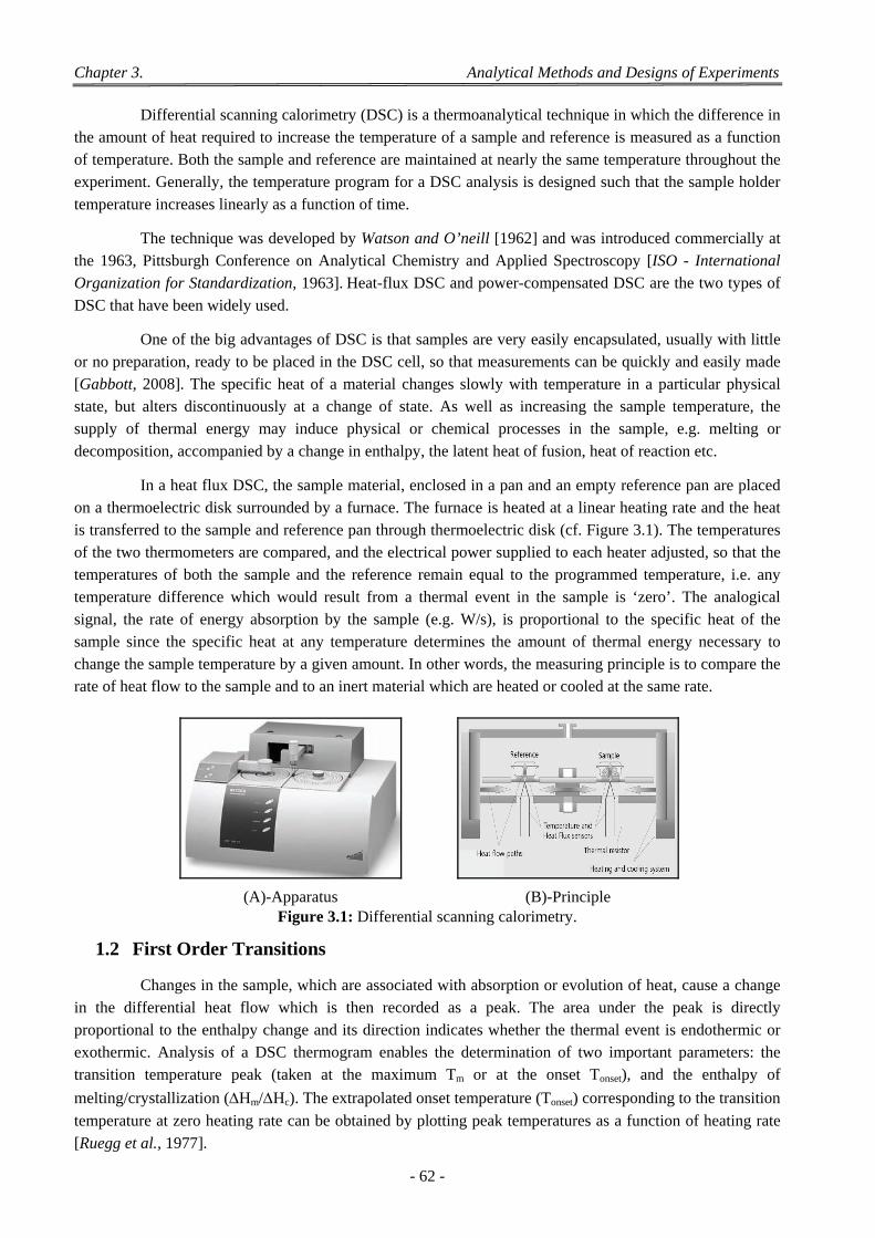
Chapter 3. Analytical Methods and Designs of Experiments
- 62 -
Differential scanning calorimetry (DSC) is a thermoanalytical technique in which the difference in the amount of heat required to increase the temperature of a sample and reference is measured as a function of temperature. Both the sample and reference are maintained at nearly the same temperature throughout the experiment. Generally, the temperature program for a DSC analysis is designed such that the sample holder
temperature increases linearly as a function of time.
The technique was developed by Watson and O’neill [1962] and was introduced commercially at the 1963, Pittsburgh Conference on Analytical Chemistry and Applied Spectroscopy [ISO - International Organization for Standardization, 1963]. Heat-flux DSC and power-compensated DSC are the two types of
DSC that have been widely used.
One of the big advantages of DSC is that samples are very easily encapsulated, usually with little or no preparation, ready to be placed in the DSC cell, so that measurements can be quickly and easily made [Gabbott, 2008]. The specific heat of a material changes slowly with temperature in a particular physical state, but alters discontinuously at a change of state. As well as increasing the sample temperature, the supply of thermal energy may induce physical or chemical processes in the sample, e.g. melting or
decomposition, accompanied by a change in enthalpy, the latent heat of fusion, heat of reaction etc.
In a heat flux DSC, the sample material, enclosed in a pan and an empty reference pan are placed on a thermoelectric disk surrounded by a furnace. The furnace is heated at a linear heating rate and the heat is transferred to the sample and reference pan through thermoelectric disk (cf. Figure 3.1). The temperatures of the two thermometers are compared, and the electrical power supplied to each heater adjusted, so that the temperatures of both the sample and the reference remain equal to the programmed temperature, i.e. any temperature difference which would result from a thermal event in the sample is ‘zero’. The analogical signal, the rate of energy absorption by the sample (e.g. W/s), is proportional to the specific heat of the sample since the specific heat at any temperature determines the amount of thermal energy necessary to change the sample temperature by a given amount. In other words, the measuring principle is to compare the rate of heat flow to the sample and to an inert material which are heated or cooled at the same rate.
(A)-Apparatus (B)-Principle
Figure 3.1: Differential scanning calorimetry.
1.2 First Order Transitions
Changes in the sample, which are associated with absorption or evolution of heat, cause a change in the differential heat flow which is then recorded as a peak. The area under the peak is directly proportional to the enthalpy change and its direction indicates whether the thermal event is endothermic or exothermic. Analysis of a DSC thermogram enables the determination of two important parameters: the transition temperature peak (taken at the maximum Tm or at the onset Tonset), and the enthalpy of
melting/crystallization (Hm/Hc). The extrapolated onset temperature (Tonset) corresponding to the transition
temperature at zero heating rate can be obtained by plotting peak temperatures as a function of heating rate
[Ruegg et al., 1977].
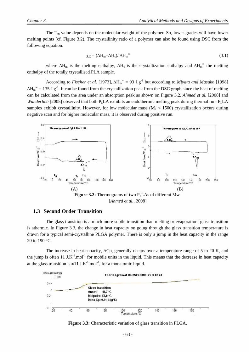
Chapter 3. Analytical Methods and Designs of Experiments
- 63 -
The Tm value depends on the molecular weight of the polymer. So, lower grades will have lower melting points (cf. Figure 3.2). The crystallinity ratio of a polymer can also be found using DSC from the
following equation:
C = (Hm−Hc)/Hm (3.1)
where Hm is the melting enthalpy, Hc is the crystallization enthalpy and Hm the melting
enthalpy of the totally crystallised PLA sample.
According to Fischer et al. [1973], Hm = 93 J.g-1 but according to Miyata and Masuko [1998]
Hm = 135 J.g-1. It can be found from the crystallization peak from the DSC graph since the heat of melting
can be calculated from the area under an absorption peak as shown on Figure 3.2. Ahmed et al. [2008] and Wunderlich [2005] observed that both PLLA exhibits an endothermic melting peak during thermal run. PLLA samples exhibit crystallinity. However, for low molecular mass (Mn < 1500) crystallization occurs during
negative scan and for higher molecular mass, it is observed during positive run.
(A) (B) Figure 3.2: Thermograms of two PLLAs of different Mw.
[Ahmed et al., 2008]
1.3 Second Order Transition
The glass transition is a much more subtle transition than melting or evaporation: glass transition is athermic. In Figure 3.3, the change in heat capacity on going through the glass transition temperature is drawn for a typical semi-crystalline PLGA polymer. There is only a jump in the heat capacity in the range
20 to 190 °C.
The increase in heat capacity, Cp, generally occurs over a temperature range of 5 to 20 K, and
the jump is often 11 J.K-1.mol-1 for mobile units in the liquid. This means that the decrease in heat capacity
at the glass transition is 11 J.K-1.mol-1, for a monatomic liquid.
Figure 3.3: Characteristic variation of glass transition in PLGA.
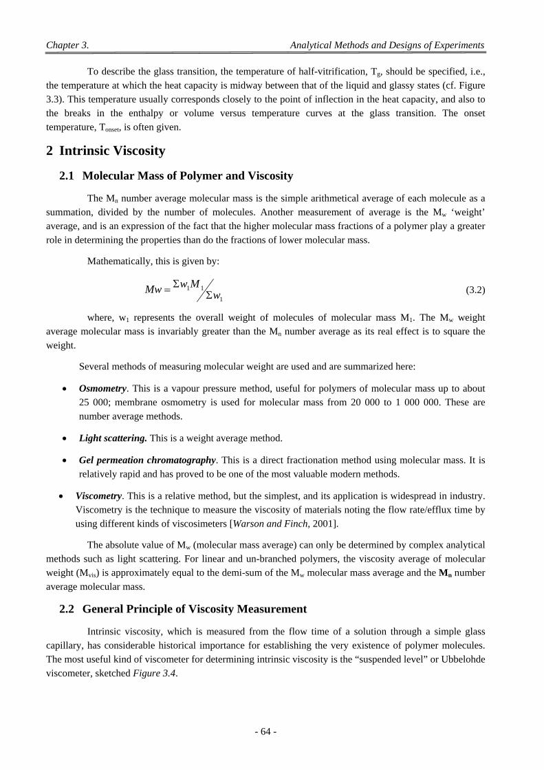
Chapter 3. Analytical Methods and Designs of Experiments
- 64 -
To describe the glass transition, the temperature of half-vitrification, Tg, should be specified, i.e., the temperature at which the heat capacity is midway between that of the liquid and glassy states (cf. Figure 3.3). This temperature usually corresponds closely to the point of inflection in the heat capacity, and also to the breaks in the enthalpy or volume versus temperature curves at the glass transition. The onset
temperature, Tonset, is often given.
2 Intrinsic Viscosity
2.1 Molecular Mass of Polymer and Viscosity
The Mn number average molecular mass is the simple arithmetical average of each molecule as a summation, divided by the number of molecules. Another measurement of average is the Mw ‘weight’ average, and is an expression of the fact that the higher molecular mass fractions of a polymer play a greater
role in determining the properties than do the fractions of lower molecular mass.
Mathematically, this is given by:
1
11w
MwMw (3.2)
where, w1 represents the overall weight of molecules of molecular mass M1. The Mw weight average molecular mass is invariably greater than the Mn number average as its real effect is to square the
weight.
Several methods of measuring molecular weight are used and are summarized here:
Osmometry. This is a vapour pressure method, useful for polymers of molecular mass up to about 25 000; membrane osmometry is used for molecular mass from 20 000 to 1 000 000. These are
number average methods.
Light scattering. This is a weight average method.
Gel permeation chromatography. This is a direct fractionation method using molecular mass. It is relatively rapid and has proved to be one of the most valuable modern methods.
Viscometry. This is a relative method, but the simplest, and its application is widespread in industry. Viscometry is the technique to measure the viscosity of materials noting the flow rate/efflux time by
using different kinds of viscosimeters [Warson and Finch, 2001].
The absolute value of Mw (molecular mass average) can only be determined by complex analytical methods such as light scattering. For linear and un-branched polymers, the viscosity average of molecular weight (Mvis) is approximately equal to the demi-sum of the Mw molecular mass average and the Mn number
average molecular mass.
2.2 General Principle of Viscosity Measurement
Intrinsic viscosity, which is measured from the flow time of a solution through a simple glass capillary, has considerable historical importance for establishing the very existence of polymer molecules. The most useful kind of viscometer for determining intrinsic viscosity is the “suspended level” or Ubbelohde
viscometer, sketched Figure 3.4.
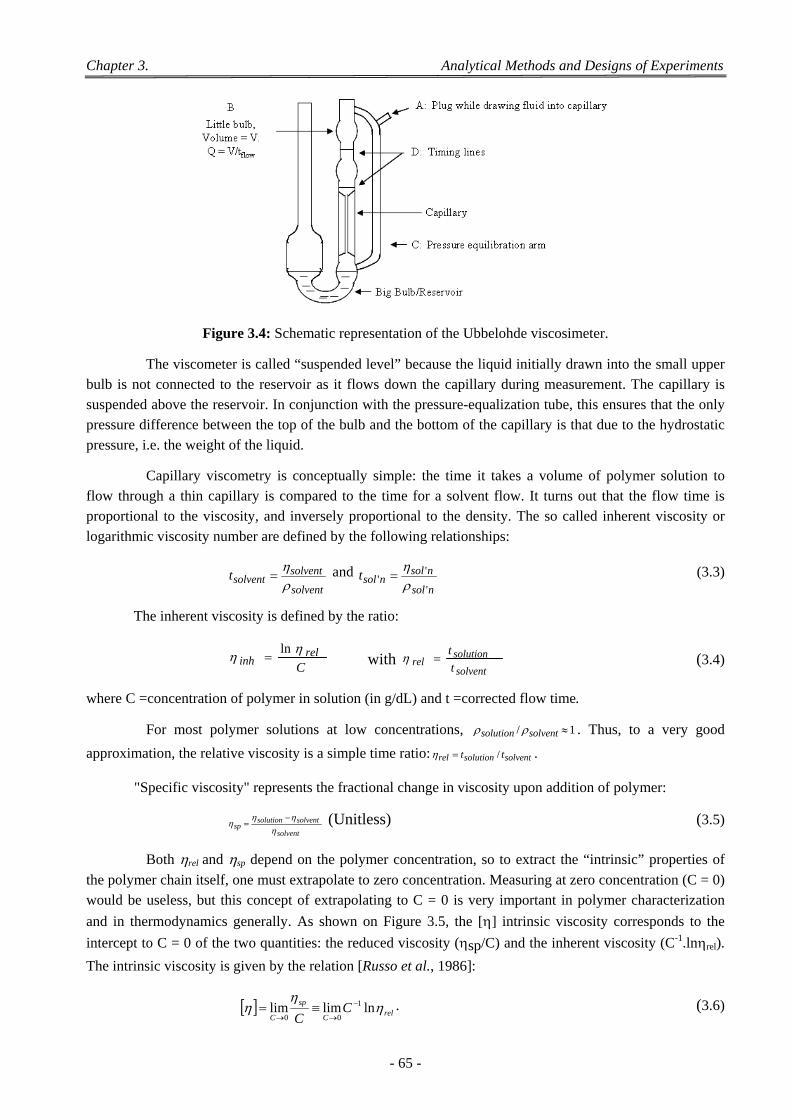
Chapter 3. Analytical Methods and Designs of Experiments
- 65 -
Figure 3.4: Schematic representation of the Ubbelohde viscosimeter.
The viscometer is called “suspended level” because the liquid initially drawn into the small upper bulb is not connected to the reservoir as it flows down the capillary during measurement. The capillary is suspended above the reservoir. In conjunction with the pressure-equalization tube, this ensures that the only pressure difference between the top of the bulb and the bottom of the capillary is that due to the hydrostatic
pressure, i.e. the weight of the liquid.
Capillary viscometry is conceptually simple: the time it takes a volume of polymer solution to flow through a thin capillary is compared to the time for a solvent flow. It turns out that the flow time is proportional to the viscosity, and inversely proportional to the density. The so called inherent viscosity or
logarithmic viscosity number are defined by the following relationships:
solvent
solventsolventt
and nsol
nsolnsolt
'
''
(3.3)
The inherent viscosity is defined by the ratio:
Crel
inh ln
with solvent
solutionrel t
t (3.4)
where C =concentration of polymer in solution (in g/dL) and t =corrected flow time.
For most polymer solutions at low concentrations, 1/ solventsolution . Thus, to a very good
approximation, the relative viscosity is a simple time ratio: solventsolutionrel tt / .
"Specific viscosity" represents the fractional change in viscosity upon addition of polymer:
solvent
solventsolutionsp
(Unitless) (3.5)
Both rel and sp depend on the polymer concentration, so to extract the “intrinsic” properties of
the polymer chain itself, one must extrapolate to zero concentration. Measuring at zero concentration (C = 0) would be useless, but this concept of extrapolating to C = 0 is very important in polymer characterization
and in thermodynamics generally. As shown on Figure 3.5, the [] intrinsic viscosity corresponds to the
intercept to C = 0 of the two quantities: the reduced viscosity (sp/C) and the inherent viscosity (C-1.lnrel).
The intrinsic viscosity is given by the relation [Russo et al., 1986]:
relC
sp
CC
C
lnlimlim 1
00
. (3.6)
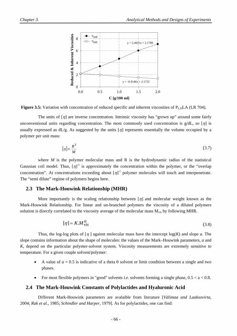
Chapter 3. Analytical Methods and Designs of Experiments
- 66 -
PLDLA-LR 704 Concentration Vs red & inh
C [g/100 ml]
0.0 0.5 1.0 1.5 2.0
Red
uce
d &
In
her
ent
Vis
cosi
ties
0
2
4
6
8y = 2.4921x + 2.1789
y = -0.4146x + 2.1725
red inh
Figure 3.5: Variation with concentration of reduced specific and inherent viscosities of PL,DLA (LR 704).
The units of [] are inverse concentration. Intrinsic viscosity has “grown up” around some fairly
unconventional units regarding concentration. The most commonly used concentration is g/dL, so [] is
usually expressed as dL/g. As suggested by the units [] represents essentially the volume occupied by a
polymer per unit mass:
M
R3 (3.7)
where M is the polymer molecular mass and R is the hydrodynamic radius of the statistical
Gaussian coil model. Thus, []-1 is approximately the concentration within the polymer, or the “overlap
concentration”. At concentrations exceeding about []-1 polymer molecules will touch and interpenetrate.
The “semi dilute” regime of polymers begins here.
2.3 The Mark-Houwink Relationship (MHR)
More importantly is the scaling relationship between [] and molecular weight known as the
Mark-Houwink Relationship. For linear and un-branched polymers the viscosity of a diluted polymers
solution is directly correlated to the viscosity average of the molecular mass Mvis by following MHR.
avisMK.][ (3.8)
Thus, the log-log plots of [] against molecular mass have the intercept log(K) and slope a. The
slope contains information about the shape of molecules: the values of the Mark–Houwink parameters, a and K, depend on the particular polymer-solvent system. Viscosity measurements are extremely sensitive to
temperature. For a given couple solvent/polymer:
A value of a = 0.5 is indicative of a theta solvent or limit condition between a single and two
phases.
For most flexible polymers in "good" solvents i.e. solvents forming a single phase, 0.5 < a < 0.8.
2.4 The Mark-Houwink Constants of Polylactides and Hyaluronic Acid
Different Mark-Houwink parameters are avalaible from literature [Välimaa and Laaksovirta,
2004; Rak et al., 1985; Schindler and Harper, 1979]. As for polylactides, one can find: .
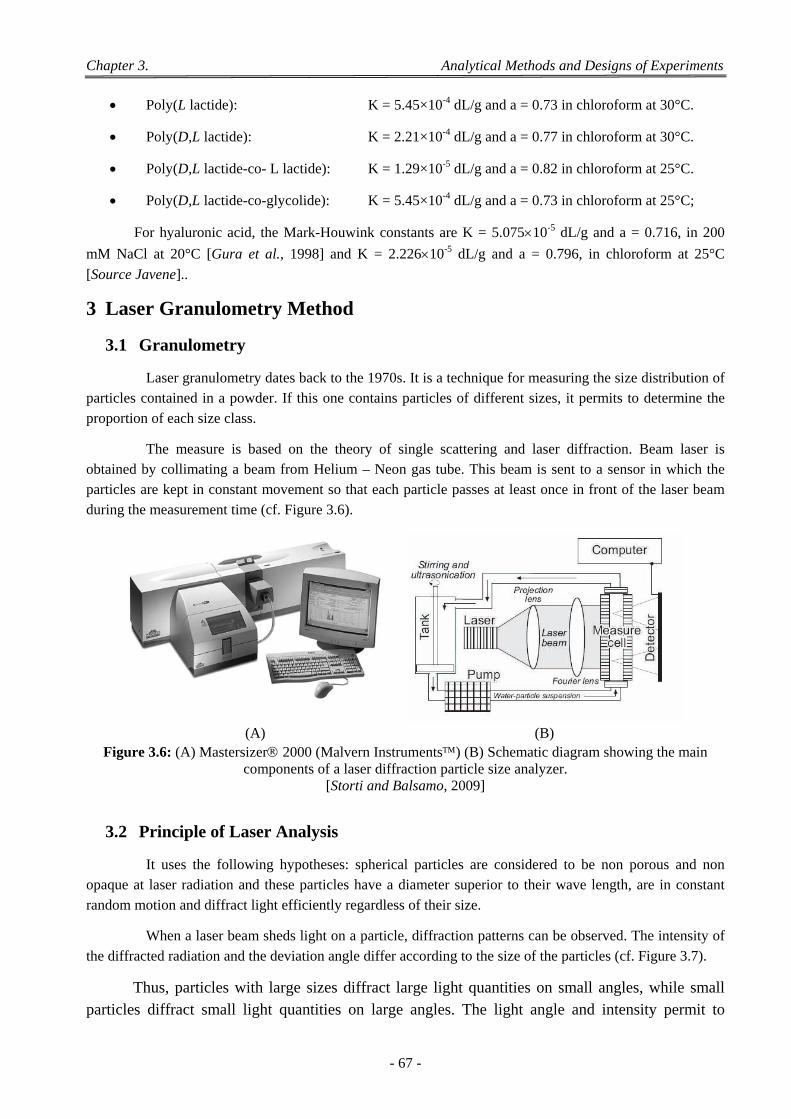
Chapter 3. Analytical Methods and Designs of Experiments
- 67 -
Poly(L lactide): K = 5.45×10⁻⁴ dL/g and a = 0.73 in chloroform at 30°C.
Poly(D,L lactide): K = 2.21×10⁻⁴ dL/g and a = 0.77 in chloroform at 30°C.
Poly(D,L lactide-co- L lactide): K = 1.29×10⁻⁵ dL/g and a = 0.82 in chloroform at 25°C.
Poly(D,L lactide-co-glycolide): K = 5.45×10⁻⁴ dL/g and a = 0.73 in chloroform at 25°C;
For hyaluronic acid, the Mark-Houwink constants are K = 5.07510-5 dL/g and a = 0.716, in 200
mM NaCl at 20°C [Gura et al., 1998] and K = 2.22610-5 dL/g and a = 0.796, in chloroform at 25°C
[Source Javene]..
3 Laser Granulometry Method
3.1 Granulometry
Laser granulometry dates back to the 1970s. It is a technique for measuring the size distribution of particles contained in a powder. If this one contains particles of different sizes, it permits to determine the
proportion of each size class.
The measure is based on the theory of single scattering and laser diffraction. Beam laser is obtained by collimating a beam from Helium – Neon gas tube. This beam is sent to a sensor in which the particles are kept in constant movement so that each particle passes at least once in front of the laser beam
during the measurement time (cf. Figure 3.6).
(A) (B) Figure 3.6: (A) Mastersizer 2000 (Malvern Instruments) (B) Schematic diagram showing the main
components of a laser diffraction particle size analyzer. [Storti and Balsamo, 2009]
3.2 Principle of Laser Analysis
It uses the following hypotheses: spherical particles are considered to be non porous and non opaque at laser radiation and these particles have a diameter superior to their wave length, are in constant
random motion and diffract light efficiently regardless of their size.
When a laser beam sheds light on a particle, diffraction patterns can be observed. The intensity of
the diffracted radiation and the deviation angle differ according to the size of the particles (cf. Figure 3.7).
Thus, particles with large sizes diffract large light quantities on small angles, while small particles diffract small light quantities on large angles. The light angle and intensity permit to
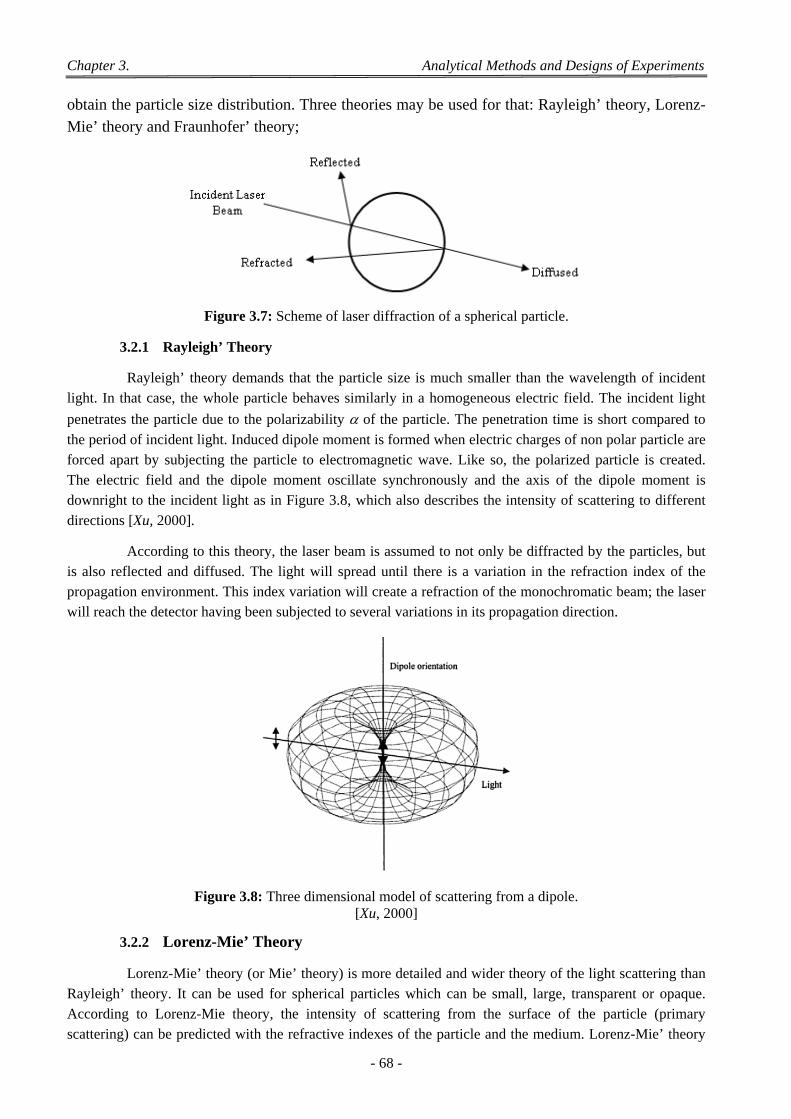
Chapter 3. Analytical Methods and Designs of Experiments
- 68 -
obtain the particle size distribution. Three theories may be used for that: Rayleigh’ theory, Lorenz-Mie’ theory and Fraunhofer’ theory;
Figure 3.7: Scheme of laser diffraction of a spherical particle.
3.2.1 Rayleigh’ Theory
Rayleigh’ theory demands that the particle size is much smaller than the wavelength of incident light. In that case, the whole particle behaves similarly in a homogeneous electric field. The incident light
penetrates the particle due to the polarizability of the particle. The penetration time is short compared to
the period of incident light. Induced dipole moment is formed when electric charges of non polar particle are forced apart by subjecting the particle to electromagnetic wave. Like so, the polarized particle is created. The electric field and the dipole moment oscillate synchronously and the axis of the dipole moment is downright to the incident light as in Figure 3.8, which also describes the intensity of scattering to different
directions [Xu, 2000].
According to this theory, the laser beam is assumed to not only be diffracted by the particles, but is also reflected and diffused. The light will spread until there is a variation in the refraction index of the propagation environment. This index variation will create a refraction of the monochromatic beam; the laser will reach the detector having been subjected to several variations in its propagation direction.
Figure 3.8: Three dimensional model of scattering from a dipole. [Xu, 2000]
3.2.2 Lorenz-Mie’ Theory
Lorenz-Mie’ theory (or Mie’ theory) is more detailed and wider theory of the light scattering than Rayleigh’ theory. It can be used for spherical particles which can be small, large, transparent or opaque. According to Lorenz-Mie theory, the intensity of scattering from the surface of the particle (primary scattering) can be predicted with the refractive indexes of the particle and the medium. Lorenz-Mie’ theory
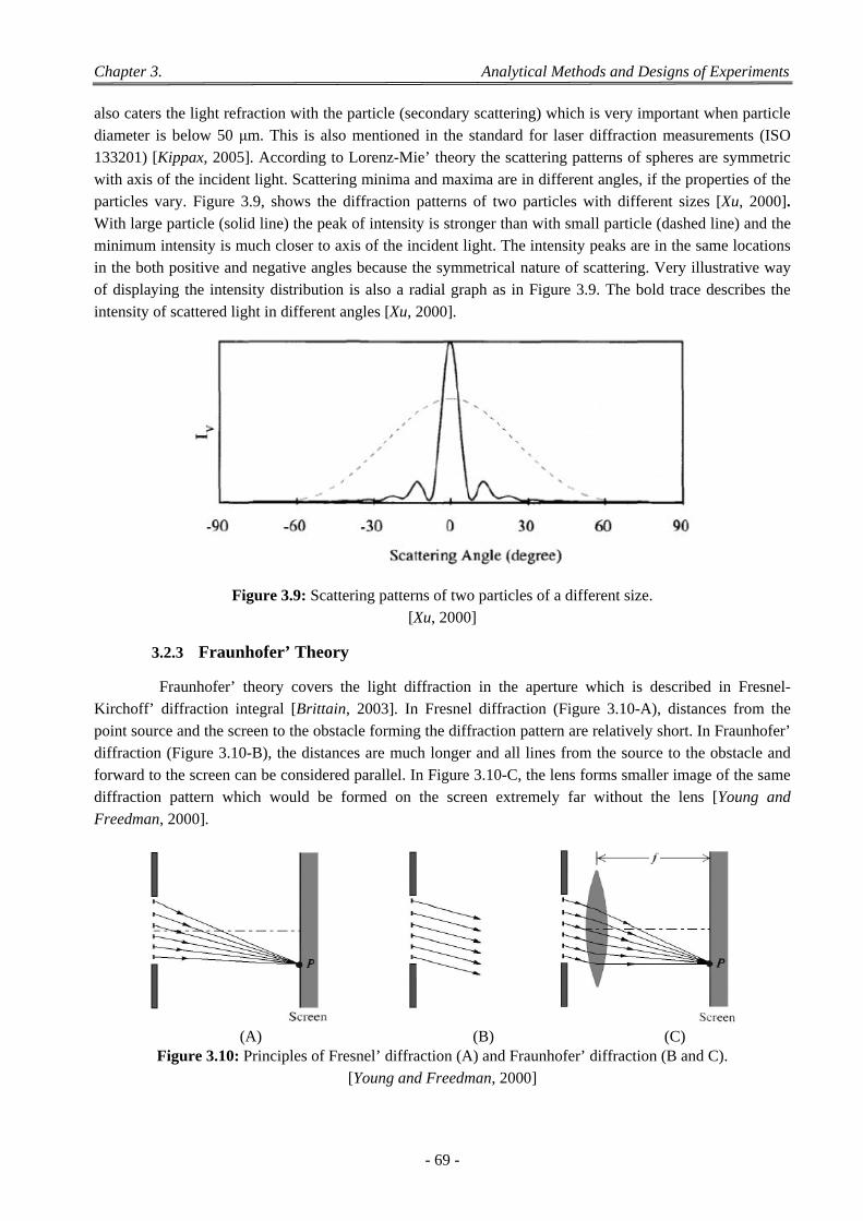
Chapter 3. Analytical Methods and Designs of Experiments
- 69 -
also caters the light refraction with the particle (secondary scattering) which is very important when particle diameter is below 50 μm. This is also mentioned in the standard for laser diffraction measurements (ISO 133201) [Kippax, 2005]. According to Lorenz-Mie’ theory the scattering patterns of spheres are symmetric with axis of the incident light. Scattering minima and maxima are in different angles, if the properties of the particles vary. Figure 3.9, shows the diffraction patterns of two particles with different sizes [Xu, 2000]. With large particle (solid line) the peak of intensity is stronger than with small particle (dashed line) and the minimum intensity is much closer to axis of the incident light. The intensity peaks are in the same locations in the both positive and negative angles because the symmetrical nature of scattering. Very illustrative way of displaying the intensity distribution is also a radial graph as in Figure 3.9. The bold trace describes the
intensity of scattered light in different angles [Xu, 2000].
Figure 3.9: Scattering patterns of two particles of a different size. [Xu, 2000]
3.2.3 Fraunhofer’ Theory
Fraunhofer’ theory covers the light diffraction in the aperture which is described in Fresnel-Kirchoff’ diffraction integral [Brittain, 2003]. In Fresnel diffraction (Figure 3.10-A), distances from the point source and the screen to the obstacle forming the diffraction pattern are relatively short. In Fraunhofer’ diffraction (Figure 3.10-B), the distances are much longer and all lines from the source to the obstacle and forward to the screen can be considered parallel. In Figure 3.10-C, the lens forms smaller image of the same diffraction pattern which would be formed on the screen extremely far without the lens [Young and
Freedman, 2000].
(A) (B) (C) Figure 3.10: Principles of Fresnel’ diffraction (A) and Fraunhofer’ diffraction (B and C).
[Young and Freedman, 2000]
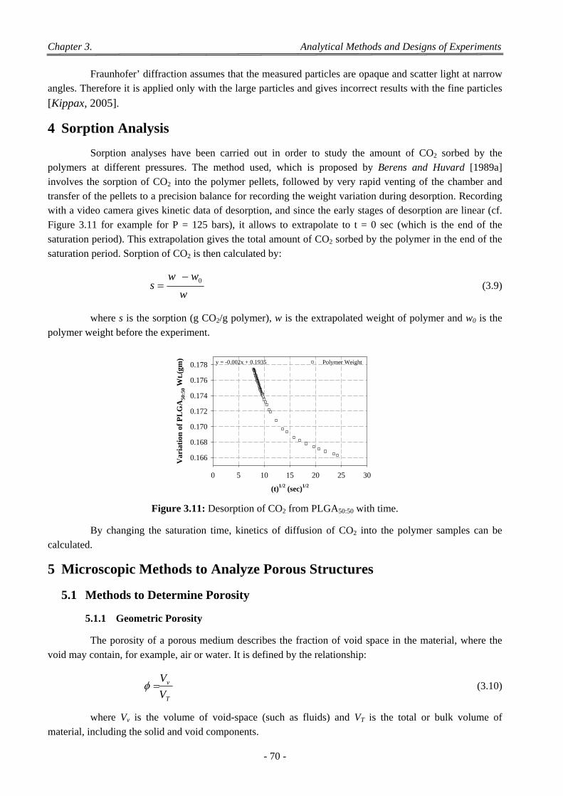
Chapter 3. Analytical Methods and Designs of Experiments
- 70 -
Fraunhofer’ diffraction assumes that the measured particles are opaque and scatter light at narrow angles. Therefore it is applied only with the large particles and gives incorrect results with the fine particles
[Kippax, 2005].
4 Sorption Analysis
Sorption analyses have been carried out in order to study the amount of CO2 sorbed by the polymers at different pressures. The method used, which is proposed by Berens and Huvard [1989a] involves the sorption of CO2 into the polymer pellets, followed by very rapid venting of the chamber and transfer of the pellets to a precision balance for recording the weight variation during desorption. Recording with a video camera gives kinetic data of desorption, and since the early stages of desorption are linear (cf. Figure 3.11 for example for P = 125 bars), it allows to extrapolate to t = 0 sec (which is the end of the saturation period). This extrapolation gives the total amount of CO2 sorbed by the polymer in the end of the
saturation period. Sorption of CO2 is then calculated by:
w
wws 0 (3.9)
where s is the sorption (g CO2/g polymer), w is the extrapolated weight of polymer and w0 is the
polymer weight before the experiment.
Extrapolated Weight of Polymer with Time
(t)1/2 (sec)1/2
0 5 10 15 20 25 30
Var
iati
on o
f P
LG
A50
:50
Wt.
(gm
)
0.166
0.168
0.170
0.172
0.174
0.176
0.178 Polymer Weighty = -0.002x + 0.1935
Figure 3.11: Desorption of CO2 from PLGA50:50 with time.
By changing the saturation time, kinetics of diffusion of CO2 into the polymer samples can be
calculated.
5 Microscopic Methods to Analyze Porous Structures
5.1 Methods to Determine Porosity
5.1.1 Geometric Porosity
The porosity of a porous medium describes the fraction of void space in the material, where the
void may contain, for example, air or water. It is defined by the relationship:
T
v
V
V (3.10)
where Vv is the volume of void-space (such as fluids) and VT is the total or bulk volume of
material, including the solid and void components.
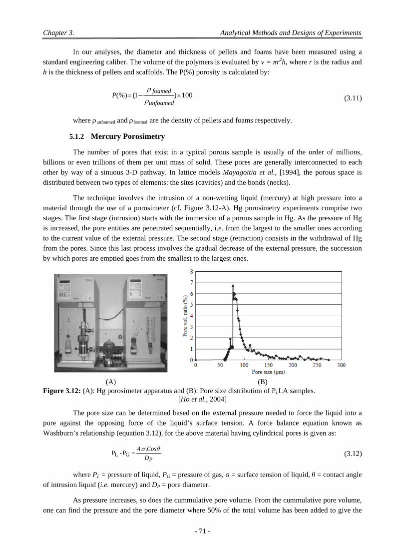
Chapter 3. Analytical Methods and Designs of Experiments
- 71 -
In our analyses, the diameter and thickness of pellets and foams have been measured using a standard engineering caliber. The volume of the polymers is evaluated by v = πr2h, where r is the radius and
h is the thickness of pellets and scaffolds. The P(%) porosity is calculated by:
100)1((%) unfoamed
foamedP
(3.11)
where unfoamed and foamed are the density of pellets and foams respectively.
5.1.2 Mercury Porosimetry
The number of pores that exist in a typical porous sample is usually of the order of millions, billions or even trillions of them per unit mass of solid. These pores are generally interconnected to each other by way of a sinuous 3-D pathway. In lattice models Mayagoitia et al., [1994], the porous space is
distributed between two types of elements: the sites (cavities) and the bonds (necks).
The technique involves the intrusion of a non-wetting liquid (mercury) at high pressure into a material through the use of a porosimeter (cf. Figure 3.12-A). Hg porosimetry experiments comprise two stages. The first stage (intrusion) starts with the immersion of a porous sample in Hg. As the pressure of Hg is increased, the pore entities are penetrated sequentially, i.e. from the largest to the smaller ones according to the current value of the external pressure. The second stage (retraction) consists in the withdrawal of Hg from the pores. Since this last process involves the gradual decrease of the external pressure, the succession
by which pores are emptied goes from the smallest to the largest ones.
(A) (B) Figure 3.12: (A): Hg porosimeter apparatus and (B): Pore size distribution of PLLA samples.
[Ho et al., 2004]
The pore size can be determined based on the external pressure needed to force the liquid into a pore against the opposing force of the liquid’s surface tension. A force balance equation known as
Washburn’s relationship (equation 3.12), for the above material having cylindrical pores is given as:
PD
Cos ..4P-P GL (3.12)
where PL = pressure of liquid, PG = pressure of gas, σ = surface tension of liquid, θ = contact angle
of intrusion liquid (i.e. mercury) and DP = pore diameter.
As pressure increases, so does the cummulative pore volume. From the cummulative pore volume, one can find the pressure and the pore diameter where 50% of the total volume has been added to give the
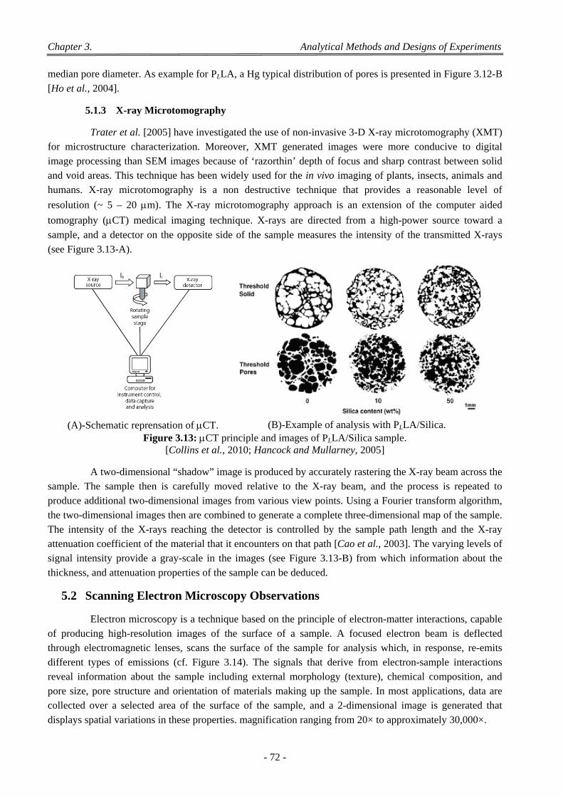
Chapter 3. Analytical Methods and Designs of Experiments
- 72 -
median pore diameter. As example for PLLA, a Hg typical distribution of pores is presented in Figure 3.12-B
[Ho et al., 2004].
5.1.3 X-ray Microtomography
Trater et al. [2005] have investigated the use of non-invasive 3-D X-ray microtomography (XMT) for microstructure characterization. Moreover, XMT generated images were more conducive to digital image processing than SEM images because of ‘razorthin’ depth of focus and sharp contrast between solid and void areas. This technique has been widely used for the in vivo imaging of plants, insects, animals and humans. X-ray microtomography is a non destructive technique that provides a reasonable level of
resolution (~ 5 – 20 m). The X-ray microtomography approach is an extension of the computer aided
tomography (CT) medical imaging technique. X-rays are directed from a high-power source toward a
sample, and a detector on the opposite side of the sample measures the intensity of the transmitted X-rays
(see Figure 3.13-A).
(A)-Schematic reprensation of CT. (B)-Example of analysis with PLLA/Silica.
Figure 3.13: CT principle and images of PLLA/Silica sample. [Collins et al., 2010; Hancock and Mullarney, 2005]
A two-dimensional “shadow” image is produced by accurately rastering the X-ray beam across the sample. The sample then is carefully moved relative to the X-ray beam, and the process is repeated to produce additional two-dimensional images from various view points. Using a Fourier transform algorithm, the two-dimensional images then are combined to generate a complete three-dimensional map of the sample. The intensity of the X-rays reaching the detector is controlled by the sample path length and the X-ray attenuation coefficient of the material that it encounters on that path [Cao et al., 2003]. The varying levels of signal intensity provide a gray-scale in the images (see Figure 3.13-B) from which information about the
thickness, and attenuation properties of the sample can be deduced.
5.2 Scanning Electron Microscopy Observations
Electron microscopy is a technique based on the principle of electron-matter interactions, capable of producing high-resolution images of the surface of a sample. A focused electron beam is deflected through electromagnetic lenses, scans the surface of the sample for analysis which, in response, re-emits different types of emissions (cf. Figure 3.14). The signals that derive from electron-sample interactions reveal information about the sample including external morphology (texture), chemical composition, and pore size, pore structure and orientation of materials making up the sample. In most applications, data are collected over a selected area of the surface of the sample, and a 2-dimensional image is generated that
displays spatial variations in these properties. magnification ranging from 20× to approximately 30,000×.
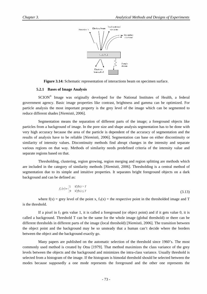
Chapter 3. Analytical Methods and Designs of Experiments
- 73 -
Figure 3.14: Schematic representation of interactions beam on specimen surface.
5.2.1 Bases of Image Analysis
SCION® Image was originally developed for the National Institutes of Health, a federal government agency. Basic image properties like contrast, brightness and gamma can be optimized. For particle analysis the most important property is the grey level of the image which can be segmented to
reduce different shades [Niemistö, 2006].
Segmentation means the separation of different parts of the image; a foreground objects like particles from a background of image. In the pore size and shape analysis segmentation has to be done with very high accuracy because the area of the particle is dependent of the accuracy of segmentation and the results of analysis have to be reliable [Niemistö, 2006]. Segmentation can base on either discontinuity or similarity of intensity values. Discontinuity methods find abrupt changes in the intensity and separate various regions on that way. Methods of similarity needs predefined criteria of the intensity value and
separate regions based on that.
Thresholding, clustering, region growing, region merging and region splitting are methods which are included in the category of similarity methods [Niemistö, 2006]. Thresholding is a central method of segmentation due to its simple and intuitive properties. It separates bright foreground objects on a dark
background and can be defined as:
(3.13)
where f(x) = grey level of the point x, fT(x) = the respective point in the thresholded image and T
is the threshold.
If a pixel in fT gets value 1, it is called a foreground (or object point) and if it gets value 0, it is called a background. Threshold T can be the same for the whole image (global threshold) or there can be different thresholds in different parts of the image (local threshold) [Niemistö, 2006]. The transition between the object point and the background may be so unsteady that a human can’t decide where the borders
between the object and the background exactly go.
Many papers are published on the automatic selection of the threshold since 1960’s. The most commonly used method is created by Otsu [1979]. That method maximizes the class variance of the grey levels between the objects and the background and minimizes the intra-class variance. Usually threshold is selected from a histogram of the image. If the histogram is bimodal threshold should be selected between the modes because supposedly a one mode represents the foreground and the other one represents the
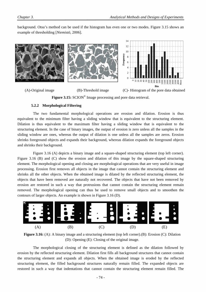
Chapter 3. Analytical Methods and Designs of Experiments
- 74 -
background. Otsu’s method can be used if the histogram has even one or two modes. Figure 3.15 shows an
example of thresholding [Niemistö, 2006].
2D Graph 4
Bin
0 10 20 30 40 50 100
200
300
400
500
1000
1500
2000
2500
3000
3500
4000
Mor
e
Fre
quen
cy
0
2
4
6
8
10
12
14
(A)-Original image (B)-Threshold image (C)- Histogram of the pore data obtained
Figure 3.15: SCION® Image processing and pore data retrieval.
5.2.2 Morphological Filtering
The two fundamental morphological operations are erosion and dilation. Erosion is thus equivalent to the minimum filter having a sliding window that is equivalent to the structuring element. Dilation is thus equivalent to the maximum filter having a sliding window that is equivalent to the structuring element. In the case of binary images, the output of erosion is zero unless all the samples in the sliding window are ones, whereas the output of dilation is one unless all the samples are zeros. Erosion shrinks foreground objects and expands their background, whereas dilation expands the foreground objects
and shrinks their background.
Figure 3.16 (A) depicts a binary image and a square-shaped structuring element (top left corner). Figure 3.16 (B) and (C) show the erosion and dilation of this image by the square-shaped structuring element. The morphological opening and closing are morphological operations that are very useful in image processing. Erosion first removes all objects in the image that cannot contain the structuring element and shrinks all the other objects. When the obtained image is dilated by the reflected structuring element, the objects that have been removed are naturally not recovered. The objects that have not been removed by erosion are restored in such a way that protrusions that cannot contain the structuring element remain removed. The morphological opening can thus be used to remove small objects and to smoothen the
contours of larger objects. An example is shown in Figure 3.16 (D).
(A) (B) (C) (D) (E)
Figure 3.16: (A): A binary image and a structuring element (top left corner).(B): Erosion (C): Dilation
(D): Opening (E): Closing of the original image.
The morphological closing of the structuring element is defined as the dilation followed by erosion by the reflected structuring element. Dilation first fills all background structures that cannot contain the structuring element and expands all objects. When the obtained image is eroded by the reflected structuring element, the filled background structures naturally remain filled. The expanded objects are restored in such a way that indentations that cannot contain the structuring element remain filled. The
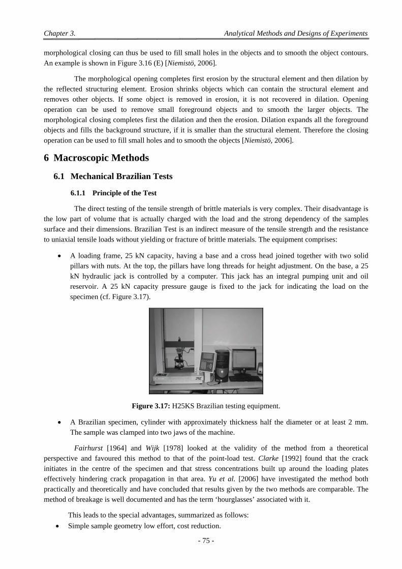
Chapter 3. Analytical Methods and Designs of Experiments
- 75 -
morphological closing can thus be used to fill small holes in the objects and to smooth the object contours.
An example is shown in Figure 3.16 (E) [Niemistö, 2006].
The morphological opening completes first erosion by the structural element and then dilation by the reflected structuring element. Erosion shrinks objects which can contain the structural element and removes other objects. If some object is removed in erosion, it is not recovered in dilation. Opening operation can be used to remove small foreground objects and to smooth the larger objects. The morphological closing completes first the dilation and then the erosion. Dilation expands all the foreground objects and fills the background structure, if it is smaller than the structural element. Therefore the closing
operation can be used to fill small holes and to smooth the objects [Niemistö, 2006].
6 Macroscopic Methods
6.1 Mechanical Brazilian Tests
6.1.1 Principle of the Test
The direct testing of the tensile strength of brittle materials is very complex. Their disadvantage is the low part of volume that is actually charged with the load and the strong dependency of the samples surface and their dimensions. Brazilian Test is an indirect measure of the tensile strength and the resistance
to uniaxial tensile loads without yielding or fracture of brittle materials. The equipment comprises:
A loading frame, 25 kN capacity, having a base and a cross head joined together with two solid pillars with nuts. At the top, the pillars have long threads for height adjustment. On the base, a 25 kN hydraulic jack is controlled by a computer. This jack has an integral pumping unit and oil reservoir. A 25 kN capacity pressure gauge is fixed to the jack for indicating the load on the
specimen (cf. Figure 3.17).
Figure 3.17: H25KS Brazilian testing equipment.
A Brazilian specimen, cylinder with approximately thickness half the diameter or at least 2 mm. The sample was clamped into two jaws of the machine.
Fairhurst [1964] and Wijk [1978] looked at the validity of the method from a theoretical perspective and favoured this method to that of the point-load test. Clarke [1992] found that the crack initiates in the centre of the specimen and that stress concentrations built up around the loading plates effectively hindering crack propagation in that area. Yu et al. [2006] have investigated the method both practically and theoretically and have concluded that results given by the two methods are comparable. The
method of breakage is well documented and has the term ‘hourglasses’ associated with it.
This leads to the special advantages, summarized as follows:
Simple sample geometry low effort, cost reduction.
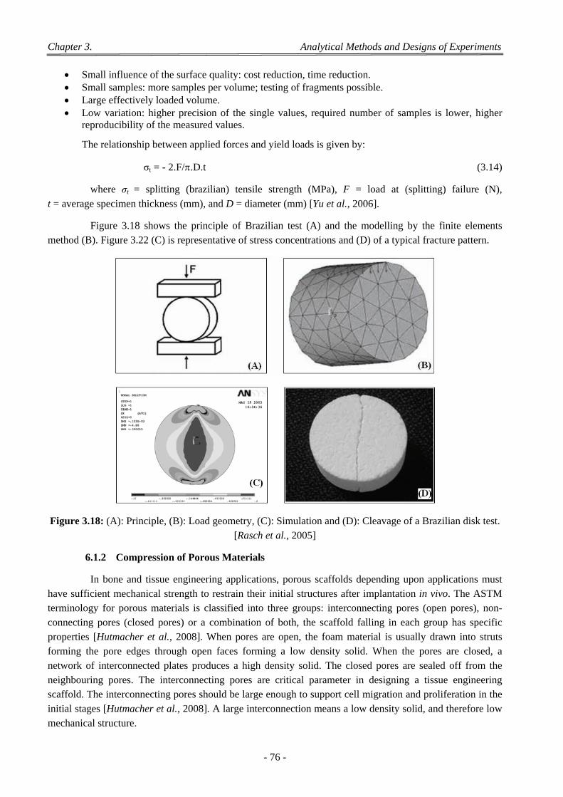
Chapter 3. Analytical Methods and Designs of Experiments
- 76 -
Small influence of the surface quality: cost reduction, time reduction. Small samples: more samples per volume; testing of fragments possible. Large effectively loaded volume. Low variation: higher precision of the single values, required number of samples is lower, higher
reproducibility of the measured values.
The relationship between applied forces and yield loads is given by:
σt = - 2.F/.D.t (3.14)
where σt = splitting (brazilian) tensile strength (MPa), F = load at (splitting) failure (N),
t = average specimen thickness (mm), and D = diameter (mm) [Yu et al., 2006].
Figure 3.18 shows the principle of Brazilian test (A) and the modelling by the finite elements method (B). Figure 3.22 (C) is representative of stress concentrations and (D) of a typical fracture pattern.
Figure 3.18: (A): Principle, (B): Load geometry, (C): Simulation and (D): Cleavage of a Brazilian disk test.
[Rasch et al., 2005]
6.1.2 Compression of Porous Materials
In bone and tissue engineering applications, porous scaffolds depending upon applications must have sufficient mechanical strength to restrain their initial structures after implantation in vivo. The ASTM terminology for porous materials is classified into three groups: interconnecting pores (open pores), non-connecting pores (closed pores) or a combination of both, the scaffold falling in each group has specific properties [Hutmacher et al., 2008]. When pores are open, the foam material is usually drawn into struts forming the pore edges through open faces forming a low density solid. When the pores are closed, a network of interconnected plates produces a high density solid. The closed pores are sealed off from the neighbouring pores. The interconnecting pores are critical parameter in designing a tissue engineering scaffold. The interconnecting pores should be large enough to support cell migration and proliferation in the initial stages [Hutmacher et al., 2008]. A large interconnection means a low density solid, and therefore low
mechanical structure.
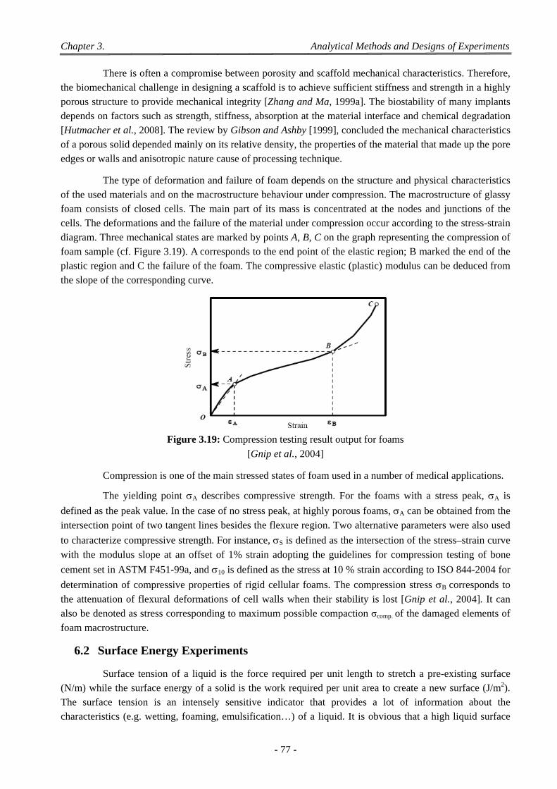
Chapter 3. Analytical Methods and Designs of Experiments
- 77 -
There is often a compromise between porosity and scaffold mechanical characteristics. Therefore, the biomechanical challenge in designing a scaffold is to achieve sufficient stiffness and strength in a highly porous structure to provide mechanical integrity [Zhang and Ma, 1999a]. The biostability of many implants depends on factors such as strength, stiffness, absorption at the material interface and chemical degradation [Hutmacher et al., 2008]. The review by Gibson and Ashby [1999], concluded the mechanical characteristics of a porous solid depended mainly on its relative density, the properties of the material that made up the pore
edges or walls and anisotropic nature cause of processing technique.
The type of deformation and failure of foam depends on the structure and physical characteristics of the used materials and on the macrostructure behaviour under compression. The macrostructure of glassy foam consists of closed cells. The main part of its mass is concentrated at the nodes and junctions of the cells. The deformations and the failure of the material under compression occur according to the stress-strain diagram. Three mechanical states are marked by points A, B, C on the graph representing the compression of foam sample (cf. Figure 3.19). A
corresponds to the end point of the elastic region; B marked the end of the
plastic region and C the failure of the foam. The compressive elastic (plastic) modulus can be deduced from
the slope of the corresponding curve.
Figure 3.19: Compression testing result output for foams
[Gnip et al., 2004]
Compression is one of the main stressed states of foam used in a number of medical applications.
The yielding point A describes compressive strength. For the foams with a stress peak, A is
defined as the peak value. In the case of no stress peak, at highly porous foams, A can be obtained from the
intersection point of two tangent lines besides the flexure region. Two alternative parameters were also used
to characterize compressive strength. For instance, S is defined as the intersection of the stress–strain curve
with the modulus slope at an offset of 1% strain adopting the guidelines for compression testing of bone
cement set in ASTM F451-99a, and 10 is defined as the stress at 10 % strain according to ISO 844-2004 for
determination of compressive properties of rigid cellular foams. The compression stress B corresponds to
the attenuation of flexural deformations of cell walls when their stability is lost [Gnip et al., 2004]. It can also be denoted as stress corresponding to maximum possible compaction σcomp. of the damaged elements of
foam macrostructure.
6.2 Surface Energy Experiments
Surface tension of a liquid is the force required per unit length to stretch a pre-existing surface (N/m) while the surface energy of a solid is the work required per unit area to create a new surface (J/m2). The surface tension is an intensely sensitive indicator that provides a lot of information about the characteristics (e.g. wetting, foaming, emulsification…) of a liquid. It is obvious that a high liquid surface
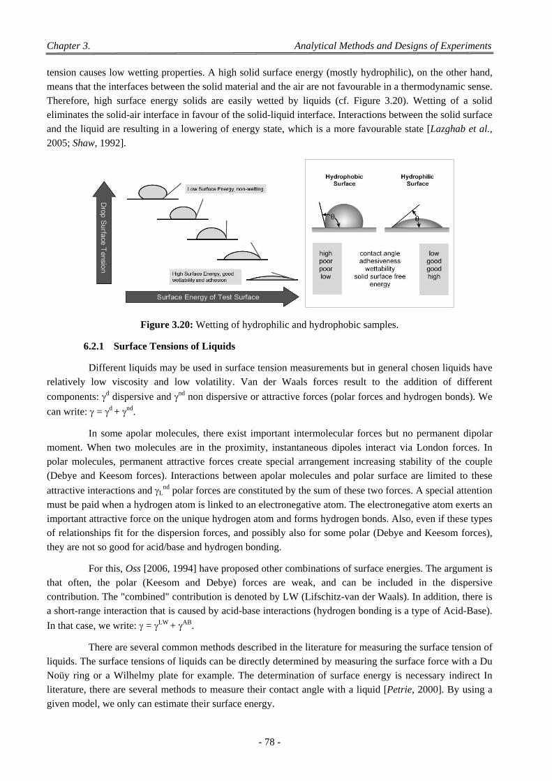
Chapter 3. Analytical Methods and Designs of Experiments
- 78 -
tension causes low wetting properties. A high solid surface energy (mostly hydrophilic), on the other hand, means that the interfaces between the solid material and the air are not favourable in a thermodynamic sense. Therefore, high surface energy solids are easily wetted by liquids (cf. Figure 3.20). Wetting of a solid eliminates the solid-air interface in favour of the solid-liquid interface. Interactions between the solid surface and the liquid are resulting in a lowering of energy state, which is a more favourable state [Lazghab et al.,
2005; Shaw, 1992].
Figure 3.20: Wetting of hydrophilic and hydrophobic samples.
6.2.1 Surface Tensions of Liquids
Different liquids may be used in surface tension measurements but in general chosen liquids have relatively low viscosity and low volatility. Van der Waals forces result to the addition of different
components: d dispersive and nd non dispersive or attractive forces (polar forces and hydrogen bonds). We
can write: = d + nd.
In some apolar molecules, there exist important intermolecular forces but no permanent dipolar moment. When two molecules are in the proximity, instantaneous dipoles interact via London forces. In polar molecules, permanent attractive forces create special arrangement increasing stability of the couple (Debye and Keesom forces). Interactions between apolar molecules and polar surface are limited to these
attractive interactions and Lnd polar forces are constituted by the sum of these two forces. A special attention
must be paid when a hydrogen atom is linked to an electronegative atom. The electronegative atom exerts an important attractive force on the unique hydrogen atom and forms hydrogen bonds. Also, even if these types of relationships fit for the dispersion forces, and possibly also for some polar (Debye and Keesom forces),
they are not so good for acid/base and hydrogen bonding.
For this, Oss [2006, 1994] have proposed other combinations of surface energies. The argument is that often, the polar (Keesom and Debye) forces are weak, and can be included in the dispersive contribution. The "combined" contribution is denoted by LW (Lifschitz-van der Waals). In addition, there is a short-range interaction that is caused by acid-base interactions (hydrogen bonding is a type of Acid-Base).
In that case, we write: = LW + AB.
There are several common methods described in the literature for measuring the surface tension of liquids. The surface tensions of liquids can be directly determined by measuring the surface force with a Du Noüy ring or a Wilhelmy plate for example. The determination of surface energy is necessary indirect In literature, there are several methods to measure their contact angle with a liquid [Petrie, 2000]. By using a
given model, we only can estimate their surface energy.
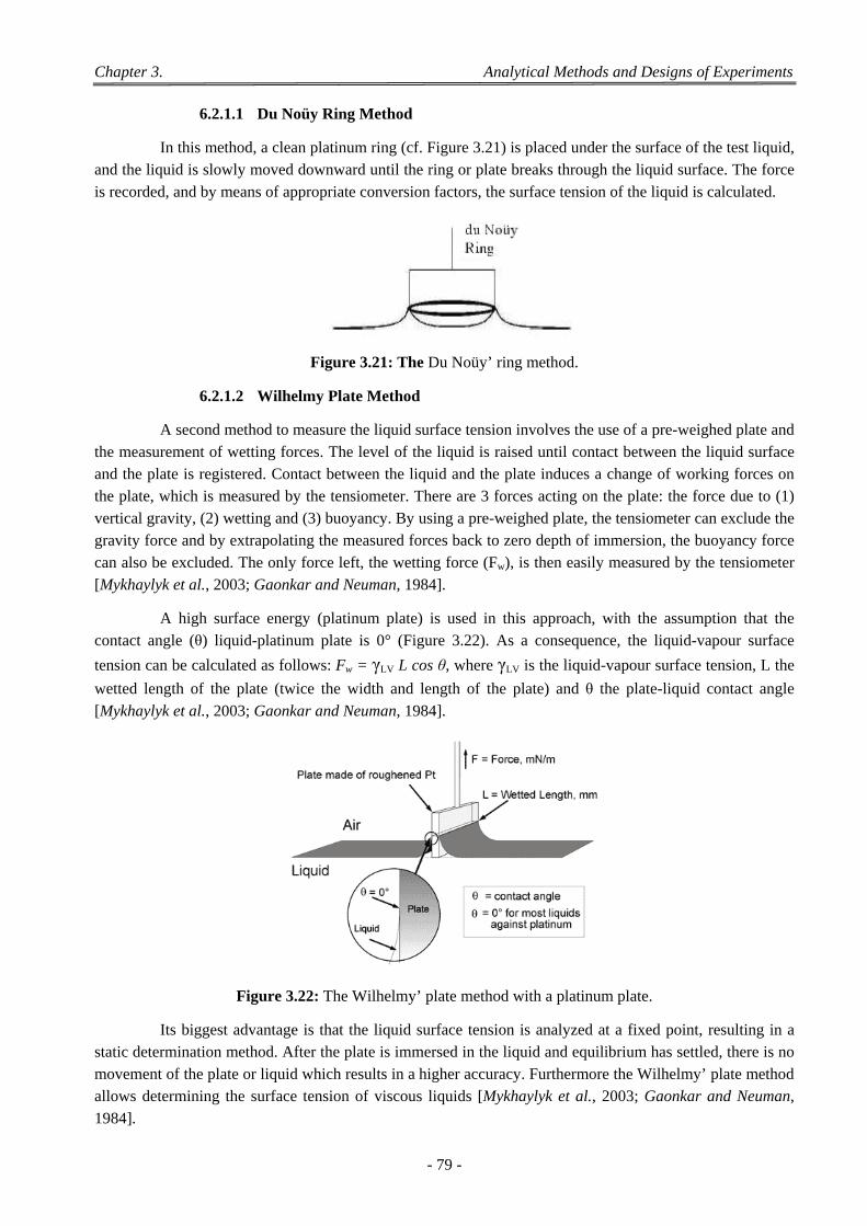
Chapter 3. Analytical Methods and Designs of Experiments
- 79 -
6.2.1.1 Du Noüy Ring Method
In this method, a clean platinum ring (cf. Figure 3.21) is placed under the surface of the test liquid, and the liquid is slowly moved downward until the ring or plate breaks through the liquid surface. The force
is recorded, and by means of appropriate conversion factors, the surface tension of the liquid is calculated.
Figure 3.21: The Du Noüy’ ring method.
6.2.1.2 Wilhelmy Plate Method
A second method to measure the liquid surface tension involves the use of a pre-weighed plate and the measurement of wetting forces. The level of the liquid is raised until contact between the liquid surface and the plate is registered. Contact between the liquid and the plate induces a change of working forces on the plate, which is measured by the tensiometer. There are 3 forces acting on the plate: the force due to (1) vertical gravity, (2) wetting and (3) buoyancy. By using a pre-weighed plate, the tensiometer can exclude the gravity force and by extrapolating the measured forces back to zero depth of immersion, the buoyancy force can also be excluded. The only force left, the wetting force (Fw), is then easily measured by the tensiometer
[Mykhaylyk et al., 2003; Gaonkar and Neuman, 1984].
A high surface energy (platinum plate) is used in this approach, with the assumption that the contact angle (θ) liquid-platinum plate is 0° (Figure 3.22). As a consequence, the liquid-vapour surface
tension can be calculated as follows: Fw = γLV L cos θ, where γLV is the liquid-vapour surface tension, L the
wetted length of the plate (twice the width and length of the plate) and θ the plate-liquid contact angle
[Mykhaylyk et al., 2003; Gaonkar and Neuman, 1984].
Figure 3.22: The Wilhelmy’ plate method with a platinum plate.
Its biggest advantage is that the liquid surface tension is analyzed at a fixed point, resulting in a static determination method. After the plate is immersed in the liquid and equilibrium has settled, there is no movement of the plate or liquid which results in a higher accuracy. Furthermore the Wilhelmy’ plate method allows determining the surface tension of viscous liquids [Mykhaylyk et al., 2003; Gaonkar and Neuman,
1984].
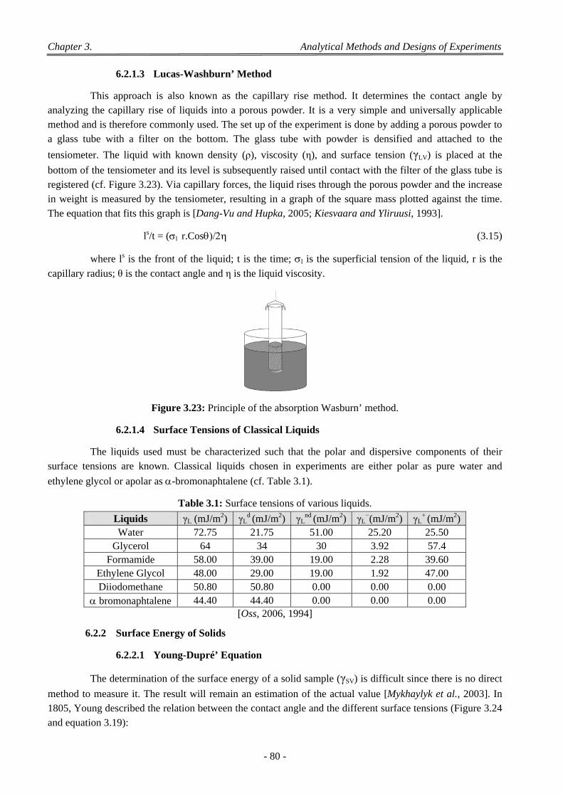
Chapter 3. Analytical Methods and Designs of Experiments
- 80 -
6.2.1.3 Lucas-Washburn’ Method
This approach is also known as the capillary rise method. It determines the contact angle by analyzing the capillary rise of liquids into a porous powder. It is a very simple and universally applicable method and is therefore commonly used. The set up of the experiment is done by adding a porous powder to a glass tube with a filter on the bottom. The glass tube with powder is densified and attached to the
tensiometer. The liquid with known density (ρ), viscosity (η), and surface tension (γLV) is placed at the
bottom of the tensiometer and its level is subsequently raised until contact with the filter of the glass tube is registered (cf. Figure 3.23). Via capillary forces, the liquid rises through the porous powder and the increase in weight is measured by the tensiometer, resulting in a graph of the square mass plotted against the time.
The equation that fits this graph is [Dang-Vu and Hupka, 2005; Kiesvaara and Yliruusi, 1993].
ls/t = (r.Cos (3.15)
where ls is the front of the liquid; t is the time; l is the superficial tension of the liquid, r is the
capillary radius; θ is the contact angle and η is the liquid viscosity.
Figure 3.23: Principle of the absorption Wasburn’ method.
6.2.1.4 Surface Tensions of Classical Liquids
The liquids used must be characterized such that the polar and dispersive components of their surface tensions are known. Classical liquids chosen in experiments are either polar as pure water and
ethylene glycol or apolar as -bromonaphtalene (cf. Table 3.1).
Table 3.1: Surface tensions of various liquids.
Liquids γL (mJ/m2) γLd (mJ/m2) γL
nd (mJ/m2) γL−(mJ/m2) γL
+ (mJ/m2)
Water 72.75 21.75 51.00 25.20 25.50 Glycerol 64 34 30 3.92 57.4
Formamide 58.00 39.00 19.00 2.28 39.60 Ethylene Glycol 48.00 29.00 19.00 1.92 47.00 Diiodomethane 50.80 50.80 0.00 0.00 0.00
bromonaphtalene 44.40 44.40 0.00 0.00 0.00 [Oss, 2006, 1994]
6.2.2 Surface Energy of Solids
6.2.2.1 Young-Dupré’ Equation
The determination of the surface energy of a solid sample (γSV) is difficult since there is no direct
method to measure it. The result will remain an estimation of the actual value [Mykhaylyk et al., 2003]. In 1805, Young described the relation between the contact angle and the different surface tensions (Figure 3.24
and equation 3.19):
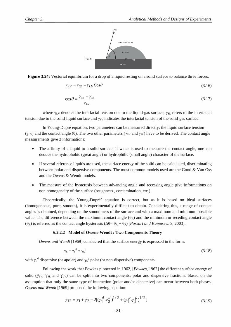
Chapter 3. Analytical Methods and Designs of Experiments
- 81 -
Figure 3.24: Vectorial equilibrium for a drop of a liquid resting on a solid surface to balance three forces.
CosLVSLSV (3.16)
LV
SLSV
cos (3.17)
where γLV denotes the interfacial tension due to the liquid-gas surface, γSL refers to the interfacial
tension due to the solid-liquid surface and γSV indicates the interfacial tension of the solid-gas surface.
In Young-Dupré equation, two parameters can be measured directly: the liquid surface tension (γLV) and the contact angle (θ). The two other parameters (γSV and γSL) have to be derived. The contact angle
measurements give 3 informations:
The affinity of a liquid to a solid surface: if water is used to measure the contact angle, one can
deduce the hydrophobic (great angle) or hydrophilic (small angle) character of the surface.
If several reference liquids are used, the surface energy of the solid can be calculated, discriminating between polar and dispersive components. The most common models used are the Good & Van Oss
and the Owens & Wendt models.
The measure of the hysteresis between advancing angle and recessing angle give informations on non homogeneity of the surface (roughness , contamination, etc.).
Theoretically, the Young-Dupré’ equation is correct, but as it is based on ideal surfaces (homogeneous, pure, smooth), it is experimentally difficult to obtain. Considering this, a range of contact angles is obtained, depending on the smoothness of the surface and with a maximum and minimum possible value. The difference between the maximum contact angle (θA) and the minimum or receding contact angle
(θR) is referred as the contact angle hysteresis (Δθ= θA − θR) [Possart and Kamusewitz, 2003].
6.2.2.2 Model of Owens-Wendt : Two Components Theory
Owens and Wendt [1969] considered that the surface energy is expressed in the form:
S = γSd + γS
p (3.18)
with γSd dispersive (or apolar) and γS
p polar (or non-dispersive) components.
Following the work that Fowkes pioneered in 1962, [Fowkes, 1962] the different surface energy of
solid (γSV, γSL and γLV) can be split into two components: polar and dispersive fractions. Based on the
assumption that only the same type of interaction (polar and/or dispersive) can occur between both phases.
Owens and Wendt [1969] proposed the following equation:
]).().[(2 2/121
2/1212112
ppdd (3.19)
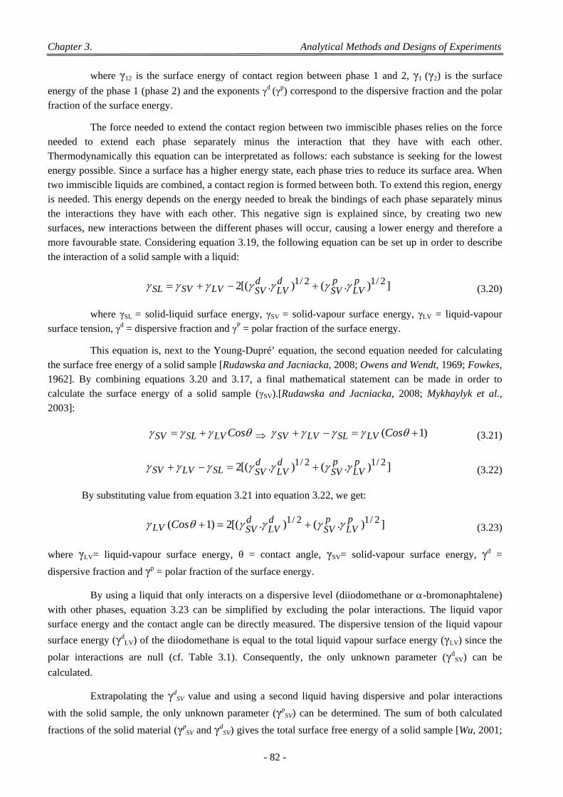
Chapter 3. Analytical Methods and Designs of Experiments
- 82 -
where γ12 is the surface energy of contact region between phase 1 and 2, γ1 (γ2) is the surface
energy of the phase 1 (phase 2) and the exponents γd (γp) correspond to the dispersive fraction and the polar
fraction of the surface energy.
The force needed to extend the contact region between two immiscible phases relies on the force needed to extend each phase separately minus the interaction that they have with each other. Thermodynamically this equation can be interpretated as follows: each substance is seeking for the lowest energy possible. Since a surface has a higher energy state, each phase tries to reduce its surface area. When two immiscible liquids are combined, a contact region is formed between both. To extend this region, energy is needed. This energy depends on the energy needed to break the bindings of each phase separately minus the interactions they have with each other. This negative sign is explained since, by creating two new surfaces, new interactions between the different phases will occur, causing a lower energy and therefore a more favourable state. Considering equation 3.19, the following equation can be set up in order to describe
the interaction of a solid sample with a liquid:
]).().[(2 2/12/1 pLV
pSV
dLV
dSVLVSVSL (3.20)
where γSL = solid-liquid surface energy, γSV = solid-vapour surface energy, γLV = liquid-vapour
surface tension, γd = dispersive fraction and γP = polar fraction of the surface energy.
This equation is, next to the Young-Dupré’ equation, the second equation needed for calculating the surface free energy of a solid sample [Rudawska and Jacniacka, 2008; Owens and Wendt, 1969; Fowkes, 1962]. By combining equations 3.20 and 3.17, a final mathematical statement can be made in order to calculate the surface energy of a solid sample (γSV).[Rudawska and Jacniacka, 2008; Mykhaylyk et al.,
2003]:
CosLVSLSV )1( CosLVSLLVSV (3.21)
]).().[(2 2/12/1 pLV
pSV
dLV
dSVSLLVSV (3.22)
By substituting value from equation 3.21 into equation 3.22, we get:
]).().[(2)1( 2/12/1 pLV
pSV
dLV
dSVLV Cos (3.23)
where γLV= liquid-vapour surface energy, θ = contact angle, γSV= solid-vapour surface energy, γd =
dispersive fraction and γp = polar fraction of the surface energy.
By using a liquid that only interacts on a dispersive level (diiodomethane or -bromonaphtalene)
with other phases, equation 3.23 can be simplified by excluding the polar interactions. The liquid vapor surface energy and the contact angle can be directly measured. The dispersive tension of the liquid vapour
surface energy (γdLV) of the diiodomethane is equal to the total liquid vapour surface energy (γLV) since the
polar interactions are null (cf. Table 3.1). Consequently, the only unknown parameter (γdSV) can be
calculated.
Extrapolating the γdSV value and using a second liquid having dispersive and polar interactions
with the solid sample, the only unknown parameter (γpSV) can be determined. The sum of both calculated
fractions of the solid material (γpSV and γd
SV) gives the total surface free energy of a solid sample [Wu, 2001;
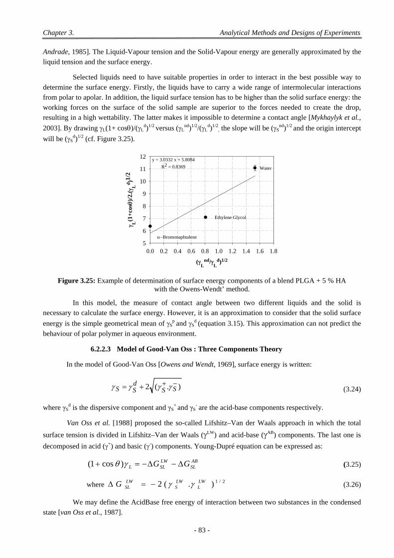
Chapter 3. Analytical Methods and Designs of Experiments
- 83 -
Andrade, 1985]. The Liquid-Vapour tension and the Solid-Vapour energy are generally approximated by the
liquid tension and the surface energy.
Selected liquids need to have suitable properties in order to interact in the best possible way to determine the surface energy. Firstly, the liquids have to carry a wide range of intermolecular interactions from polar to apolar. In addition, the liquid surface tension has to be higher than the solid surface energy: the working forces on the surface of the solid sample are superior to the forces needed to create the drop, resulting in a high wettability. The latter makes it impossible to determine a contact angle [Mykhaylyk et al.,
2003]. By drawing L(1+ cos)/(Ld)1/2 versus (L
nd)1/2/(Ld)1/2
, the slope will be (Snd)1/2
and the origin intercept
will be (Sd)1/2 (cf. Figure 3.25).
(L
nd/L
d)1/2
0.0 0.2 0.4 0.6 0.8 1.0 1.2 1.4 1.6 1.8
L(1
+co
s )/
2.(
Ld)1
/2
5
6
7
8
9
10
11
12 y = 3.0332 x + 5.8084
R2 = 0.8369 Water
romonaphtalene
Ethylene Glycol
Figure 3.25: Example of determination of surface energy components of a blend PLGA + 5 % HA with the Owens-Wendt’ method.
In this model, the measure of contact angle between two different liquids and the solid is necessary to calculate the surface energy. However, it is an approximation to consider that the solid surface
energy is the simple geometrical mean of Sp
and Sd
(equation 3.15). This approximation can not predict the
behaviour of polar polymer in aqueous environment.
6.2.2.3 Model of Good-Van Oss : Three Components Theory
In the model of Good-Van Oss [Owens and Wendt, 1969], surface energy is written:
).(2 SSdSS (3.24)
where γSd is the dispersive component and γS
+ and γS- are the acid-base components respectively.
Van Oss et al. [1988] proposed the so-called Lifshitz–Van der Waals approach in which the total
surface tension is divided in Lifshitz–Van der Waals (LW) and acid-base (AB) components. The last one is
decomposed in acid (+) and basic (-) components. Young-Dupré equation can be expressed as:
ABSL
LWSLL GG )cos1( (3.25)
where 2/1).(2 LWL
LWS
LWSLG (3.26)
We may define the AcidBase free energy of interaction between two substances in the condensed
state [van Oss et al., 1987].
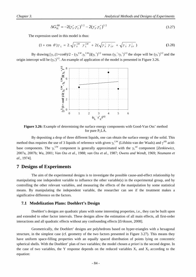
Chapter 3. Analytical Methods and Designs of Experiments
- 84 -
2/12/1 ).(2).(2 LSLSABSLG (3.27)
The expression used in this model is thus:
)(2.2)cos1( LVSLVSLWL
LWSL (3.28)
By drawing L.(1+cos)/2 - (SLW.L
LW)](L+)1/2 versus (L
−/L+)1/2
the slope will be (S+)1/2
and the
origin intercept will be (S-)1/2. An example of application of the model is presented in Figure 3.26.
(L
_
L
)1/20 1 2 3 4 5 6
L
(1+
cos
)/2(
SL
W.
LL
W)]
( L
+)1/
2
0
2
4
6
8
Figure 3.26: Example of determining the surface energy components with Good-Van Oss’ method for pure PLLA.
By depositing a drop of three different liquids, one can obtain the surface energy of the solid. This
method thus requires the use of 3 liquids of reference with given LLW (Lifshitz-van der Waals) and AB acid-
base components. The LLW component is generally approximated with the L
nd component [Zenkiewicz,
2007a, 2007b; Wu, 2001; Van Oss et al., 1988; van Oss et al., 1987; Owens and Wendt, 1969; Neumann et
al., 1974].
7 Designs of Experiments
The aim of the experimental designs is to investigate the possible cause-and-effect relationship by manipulating one independent variable to influence the other variable(s) in the experimental group, and by controlling the other relevant variables, and measuring the effects of the manipulation by some statistical means. By manipulating the independent variable, the researcher can see if the treatment makes a
significative difference on the factors.
7.1 Modelization Plans: Doehlert’s Design
Doehlert’s designs are quadratic plans with some interesting properties, i.e., they can be built upon and extended to other factor intervals. These designs allow the estimation of all main effects, all first-order
interactions and all quadratic effects without any confounding effects [Eriksson, 2008].
Geometrically, the Doehlert’ designs are polyhedrons based on hyper-triangles with a hexagonal structure, in the simplest case (cf. geometry of the two factors presented in Figure 3.27). This means they have uniform space-filling properties with an equally spaced distribution of points lying on concentric spherical shells. With the Doehlert’ plan of two variables; the model chosen a priori is the second degree. In the case of two variables, the Y response depends on the reduced variables X1 and X2 according to the
equation:
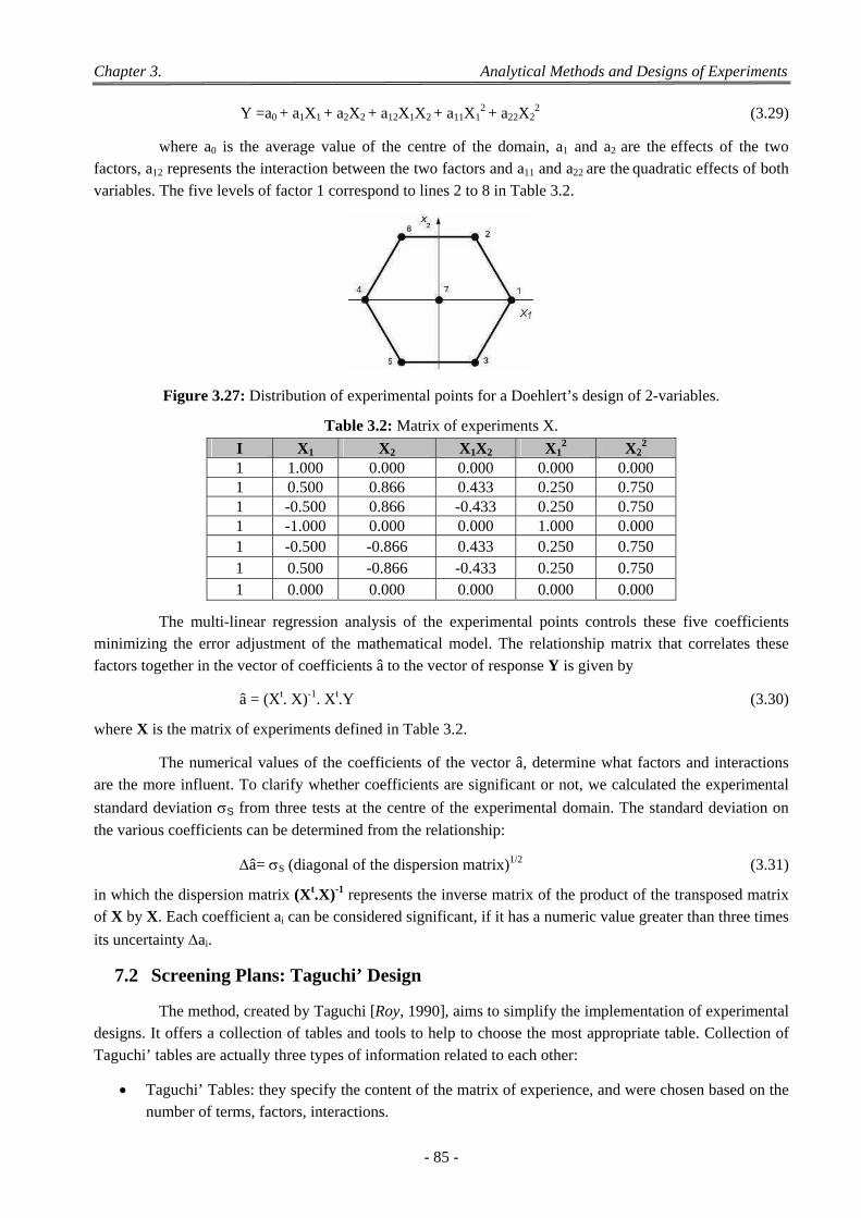
Chapter 3. Analytical Methods and Designs of Experiments
- 85 -
Y =a0 + a1X1 + a2X2 + a12X1X2 + a11X12 + a22X2
2 (3.29)
where a0 is the average value of the centre of the domain, a1 and a2 are the effects of the two factors, a12 represents the interaction between the two factors and a11 and a22 are the quadratic effects of both
variables. The five levels of factor 1 correspond to lines 2 to 8 in Table 3.2.
Figure 3.27: Distribution of experimental points for a Doehlert’s design of 2-variables.
Table 3.2: Matrix of experiments X.
I X1 X2 X1X2 X12 X2
2 1 1.000 0.000 0.000 0.000 0.000 1 0.500 0.866 0.433 0.250 0.750 1 -0.500 0.866 -0.433 0.250 0.750 1 -1.000 0.000 0.000 1.000 0.000 1 -0.500 -0.866 0.433 0.250 0.750 1 0.500 -0.866 -0.433 0.250 0.750 1 0.000 0.000 0.000 0.000 0.000
The multi-linear regression analysis of the experimental points controls these five coefficients minimizing the error adjustment of the mathematical model. The relationship matrix that correlates these
factors together in the vector of coefficients â to the vector of response Y is given by
â = (Xt. X)-1. Xt.Y (3.30)
where X is the matrix of experiments defined in Table 3.2.
The numerical values of the coefficients of the vector â, determine what factors and interactions are the more influent. To clarify whether coefficients are significant or not, we calculated the experimental
standard deviation S from three tests at the centre of the experimental domain. The standard deviation on
the various coefficients can be determined from the relationship:
â= S (diagonal of the dispersion matrix)1/2 (3.31)
in which the dispersion matrix (Xt.X)-1 represents the inverse matrix of the product of the transposed matrix of X by X. Each coefficient ai can be considered significant, if it has a numeric value greater than three times
its uncertainty ai.
7.2 Screening Plans: Taguchi’ Design
The method, created by Taguchi [Roy, 1990], aims to simplify the implementation of experimental designs. It offers a collection of tables and tools to help to choose the most appropriate table. Collection of
Taguchi’ tables are actually three types of information related to each other:
Taguchi’ Tables: they specify the content of the matrix of experience, and were chosen based on the number of terms, factors, interactions.
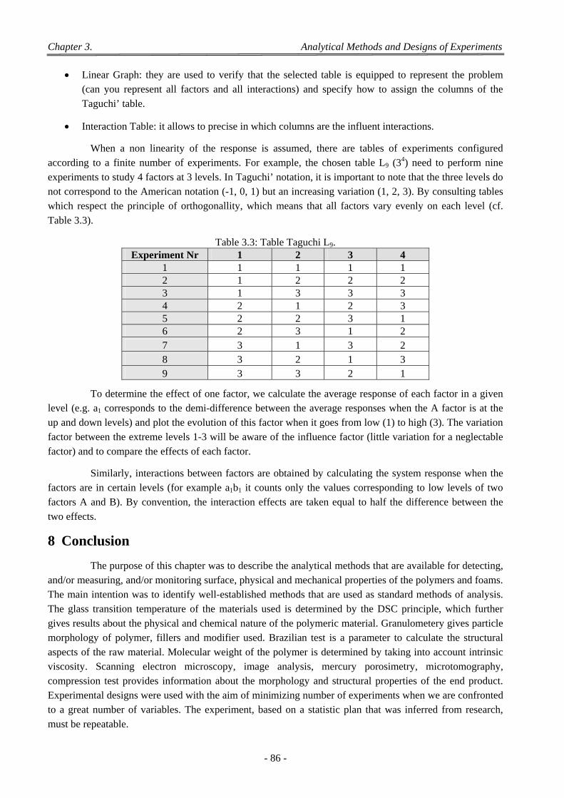
Chapter 3. Analytical Methods and Designs of Experiments
- 86 -
Linear Graph: they are used to verify that the selected table is equipped to represent the problem (can you represent all factors and all interactions) and specify how to assign the columns of the
Taguchi’ table.
Interaction Table: it allows to precise in which columns are the influent interactions.
When a non linearity of the response is assumed, there are tables of experiments configured according to a finite number of experiments. For example, the chosen table L9 (34) need to perform nine experiments to study 4 factors at 3 levels. In Taguchi’ notation, it is important to note that the three levels do not correspond to the American notation (-1, 0, 1) but an increasing variation (1, 2, 3). By consulting tables which respect the principle of orthogonallity, which means that all factors vary evenly on each level (cf.
Table 3.3).
Table 3.3: Table Taguchi L9. Experiment Nr 1 2 3 4
1 1 1 1 1 2 1 2 2 2 3 1 3 3 3 4 2 1 2 3 5 2 2 3 1 6 2 3 1 2 7 3 1 3 2 8 3 2 1 3 9 3 3 2 1
To determine the effect of one factor, we calculate the average response of each factor in a given level (e.g. a1 corresponds to the demi-difference between the average responses when the A factor is at the up and down levels) and plot the evolution of this factor when it goes from low (1) to high (3). The variation factor between the extreme levels 1-3 will be aware of the influence factor (little variation for a neglectable
factor) and to compare the effects of each factor.
Similarly, interactions between factors are obtained by calculating the system response when the factors are in certain levels (for example a1b1 it counts only the values corresponding to low levels of two factors A and B). By convention, the interaction effects are taken equal to half the difference between the
two effects.
8 Conclusion
The purpose of this chapter was to describe the analytical methods that are available for detecting, and/or measuring, and/or monitoring surface, physical and mechanical properties of the polymers and foams. The main intention was to identify well-established methods that are used as standard methods of analysis. The glass transition temperature of the materials used is determined by the DSC principle, which further gives results about the physical and chemical nature of the polymeric material. Granulometery gives particle morphology of polymer, fillers and modifier used. Brazilian test is a parameter to calculate the structural aspects of the raw material. Molecular weight of the polymer is determined by taking into account intrinsic viscosity. Scanning electron microscopy, image analysis, mercury porosimetry, microtomography, compression test provides information about the morphology and structural properties of the end product. Experimental designs were used with the aim of minimizing number of experiments when we are confronted to a great number of variables. The experiment, based on a statistic plan that was inferred from research,
must be repeatable.
Chapter 4
Chapter 4
Experimental Procedures and
Protocols for Analyses
This chapter will be devoted to the description of various experimental procedures and techniques applied for the raw materials and products used in the entire thesis. Procedures such as mixing of materials, pre-grinding by knife mill, co-grinding by tumbling ball mill and preparation of pellets by wet and dry methods will be laid down step by step. The specific conditions of various analysis techniques used to characterize the properties of the raw materials, intermediate products and final products will be presented. Procedures for laser granulometry to verify particle size, scanning electron microscopy (SEM) for observing the pore morphology and SCION® Image analysis for pore structure and their distribution will be explained
extensively. Finally, Brazilian test to identify the mechanical properties of the raw materials and
compression test will be revealed with the help of schematic diagrams.
1 Procedure for Size Reduction
Reduction of size of polymers and composites was realized in the laboratory: "Laboratoire de Génie Chimique". Biopolymers, adjuvants and fillers mixtures were prepared by two different methods, called dry and wet method. Some initial steps were common for both methods, such as size reduction, co-
grinding and mixing.
1.1 Size Reduction
1.1.1 Size Reduction by Knife Mill
Since some polylactides were supplied in the form of granules of one to several millimeters or in the form of long fibres, they were first fragmented and reduced to powders or small fibres with a laboratory
knife mill (Janke and Kunkel IKA A-10 (115 Volts), Labortechnik, Staufen, Germany).
The mill in Figure 4.1 was used for rapid, high-speed grinding of small samples from 10 to 25
gms. This apparatus can grind samples down to few hundreds of μm in seconds depending upon the nature of material. Stainless steel or hard-faced blade rotates at speeds up to 20000 rpm. Temperature is maintained by means of built-in heat exchangers and the control panel has an overload protection reset button and a
pilot light. Tubing connections 6.4 mm on the cover and housing accept tubes for circulating water.
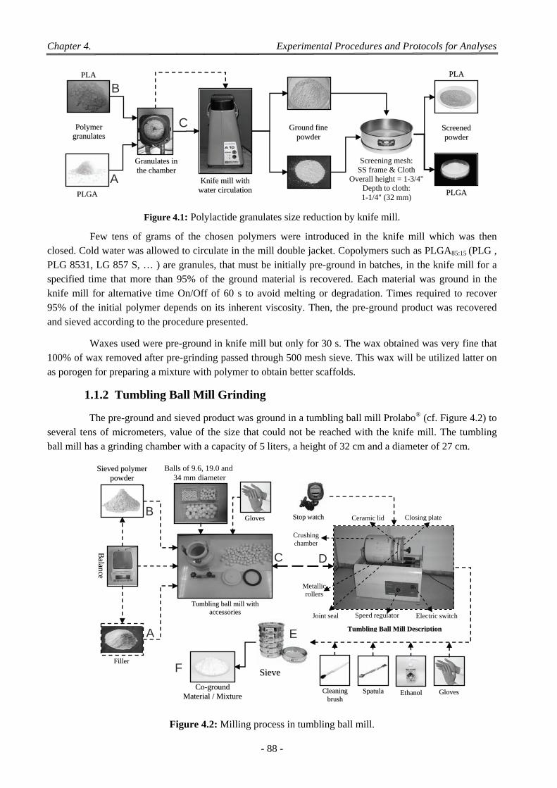
Chapter 4. Experimental Procedures and Protocols for Analyses
- 88 -
Figure 4.1: Polylactide granulates size reduction by knife mill.
Few tens of grams of the chosen polymers were introduced in the knife mill which was then closed. Cold water was allowed to circulate in the mill double jacket. Copolymers such as PLGA85:15 (PLG , PLG 8531, LG 857 S, … ) are granules, that must be initially pre-ground in batches, in the knife mill for a specified time that more than 95% of the ground material is recovered. Each material was ground in the knife mill for alternative time On/Off of 60 s to avoid melting or degradation. Times required to recover 95% of the initial polymer depends on its inherent viscosity. Then, the pre-ground product was recovered
and sieved according to the procedure presented.
Waxes used were pre-ground in knife mill but only for 30 s. The wax obtained was very fine that 100% of wax removed after pre-grinding passed through 500 mesh sieve. This wax will be utilized latter on
as porogen for preparing a mixture with polymer to obtain better scaffolds.
1.1.2 Tumbling Ball Mill Grinding
The pre-ground and sieved product was ground in a tumbling ball mill Prolabo® (cf. Figure 4.2) to several tens of micrometers, value of the size that could not be reached with the knife mill. The tumbling
ball mill has a grinding chamber with a capacity of 5 liters, a height of 32 cm and a diameter of 27 cm.
Figure 4.2: Milling process in tumbling ball mill.
TTuummbblliinngg bbaallll mmiillll wwiitthh aacccceessssoorriieess
FFiilllleerr
SSttoopp wwaattcchh
Crushing chamber
Ceramic lid
Electric switch Joint seal
Metallic rollers
Speed regulator
Closing plate
TTuummbblliinngg BBaallll MMiillll DDeessccrriippttiioonn
GGlloovveess
GGlloovveess CClleeaanniinngg bbrruusshh
SSppaattuullaa
SSiieevvee
A
B
C D
E
F
EEtthhaannooll
Balls of 9.6, 19.0 and 34 mm diameter
BBaa ll aa nn cc ee
CCoo--ggrroouunndd MMaatteerriiaall // MMiixxttuurree
SSiieevveedd ppoollyymmeerr ppoowwddeerr
Screening mesh: SS frame & Cloth
Overall height = 1-3/4" Depth to cloth: 1-1/4" (32 mm)
PPLLAA
GGrraannuullaatteess iinn tthhee cchhaammbbeerr
KKnniiffee mmiillll wwiitthh wwaatteerr cciirrccuullaattiioonn
GGrroouunndd ffiinnee ppoowwddeerr
PPoollyymmeerr ggrraannuullaatteess
PPLLGGAA
SSccrreeeenneedd ppoowwddeerr
PPLLAA
PPLLGGAA
A
B
C
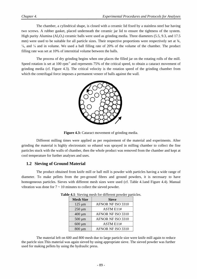
Chapter 4. Experimental Procedures and Protocols for Analyses
- 89 -
The chamber, a cylindrical shape, is closed with a ceramic lid fixed by a stainless steel bar having two screws. A rubber gasket, placed underneath the ceramic jar lid to ensure the tightness of the system. High purity Alumina (Al2O3) ceramic balls were used as grinding media. Three diameters (5.5, 9.3, and 17.5 mm) were used to be suitable for all particle sizes. Their respective proportions were respectively set at ¾, ⅛, and ⅛ and in volume. We used a ball filling rate of 20% of the volume of the chamber. The product
filling rate was set at 10% of interstitial volume between the balls.
The process of dry grinding begins when one places the filled jar on the rotating rolls of the mill. Speed rotation is set at 100 rpm-1 and represents 75% of the critical speed, to obtain a cataract movement of grinding media (cf. Figure 4.3). The critical velocity is the rotation speed of the grinding chamber from
which the centrifugal force imposes a permanent veneer of balls against the wall.
Figure 4.3: Cataract movement of grinding media.
Different milling times were applied as per requirement of the material and experiments. After grinding the material is highly electrostatic so ethanol was sprayed in milling chamber to collect the fine particles stuck with the walls of chamber, then the whole product was removed from the chamber and kept at
cool temperature for further analyses and uses.
1.2 Sieving of Ground Material
The product obtained from knife mill or ball mill is powder with particles having a wide range of diameter. To make pellets from the pre-ground fibres and ground powders, it is necessary to have homogeneous particles. Sieves with different mesh sizes were used (cf. Table 4.1and Figure 4.4). Manual
vibration was done for 7 ~ 10 minutes to collect the sieved powder.
Table 4.1: Sieving mesh for different powder particles. Mesh Size Sieve
125 μm AFNOR NF ISO 3310 250 μm ASTM E11# 400 μm AFNOR NF ISO 3310 500 μm AFNOR NF ISO 3310 600 μm ASTM E11# 800 μm AFNOR NF ISO 3310
The material left on 600 and 800 mesh due to large particle size were knife mill again to reduce
the paricle size.This material was again sieved by using appropriate sieve. The sieved powder was further used for making pellets by using the hydraulic press.
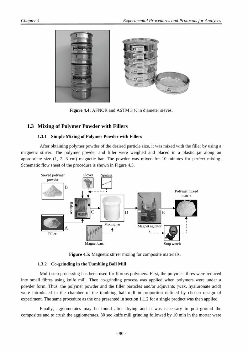
Chapter 4. Experimental Procedures and Protocols for Analyses
- 90 -
Figure 4.4: AFNOR and ASTM 3 ½ in diameter sieves.
1.3 Mixing of Polymer Powder with Fillers
1.3.1 Simple Mixing of Polymer Powder with Fillers
After obtaining polymer powder of the desired particle size, it was mixed with the filler by using a magnetic stirrer. The polymer powder and filler were weighed and placed in a plastic jar along an appropriate size (1, 2, 3 cm) magnetic bar. The powder was mixed for 10 minutes for perfect mixing.
Schematic flow sheet of the procedure is shown in Figure 4.5.
Figure 4.5: Magnetic stirrer mixing for composite materials.
1.3.2 Co-grinding in the Tumbling Ball Mill
Multi step processing has been used for fibrous polymers. First, the polymer fibres were reduced into small fibres using knife mill. Then co-grinding process was applied when polymers were under a powder form. Thus, the polymer powder and the filler particles and/or adjuvants (wax, hyaluronate acid) were introduced in the chamber of the tumbling ball mill in proportion defined by chosen design of
experiment. The same procedure as the one presented in section 1.1.2 for a single product was then applied.
Finally, agglomerates may be found after drying and it was necessary to post-ground the composites and to crush the agglomerates. 30 sec knife mill grinding followed by 10 min in the mortar were
FFiilllleerr
MMaaggnneett bbaarrss
MMaaggnneett aaggiittaattoorr
PPoollyymmeerr mmiixxeedd mmaattrriixx
MMiixxiinngg jjaarr
SSttoopp wwaattcchh
BBaa ll aa nn cc ee
GGlloovveess SSppaattuullaa
A
B
D E C
SSiieevveedd ppoollyymmeerr ppoowwddeerr
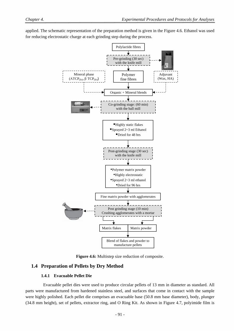
Chapter 4. Experimental Procedures and Protocols for Analyses
- 91 -
applied. The schematic representation of the preparation method is given in the Figure 4.6. Ethanol was used
for reducing electrostatic charge at each grinding step during the process.
Figure 4.6: Multistep size reduction of composite.
1.4 Preparation of Pellets by Dry Method
1.4.1 Evacuable Pellet Die
Evacuable pellet dies were used to produce circular pellets of 13 mm in diameter as standard. All parts were manufactured from hardened stainless steel, and surfaces that come in contact with the sample were highly polished. Each pellet die comprises an evacuable base (50.8 mm base diameter), body, plunger (34.8 mm height), set of pellets, extractor ring, and O Ring Kit. As shown in Figure 4.7, polyimide film is
Polylactide fibres
Polymer fine fibres
Mineral phase (TCP(Sr), TCP(Sr))
Organic + Mineral blends
•Polymer matrix powder
•Highly electrostatic
•Sprayed 2~3 ml ethanol
•Dried for 96 hrs
Post-grinding stage (30 sec) with the knife mill
Fine matrix powder with agglomerates
Post grinding stage (10 min) Crushing agglomerates with a mortar
Pre-grinding (30 sec) with the knife mill
Co-grinding stage: (60 min) with the ball mill
Highly static flakes
Sprayed 2~3 ml Ethanol
Dried for 48 hrs
Blend of flakes and powder to manufacture pellets
Matrix powderMatrix flakes
Adjuvant (Wax, HA)
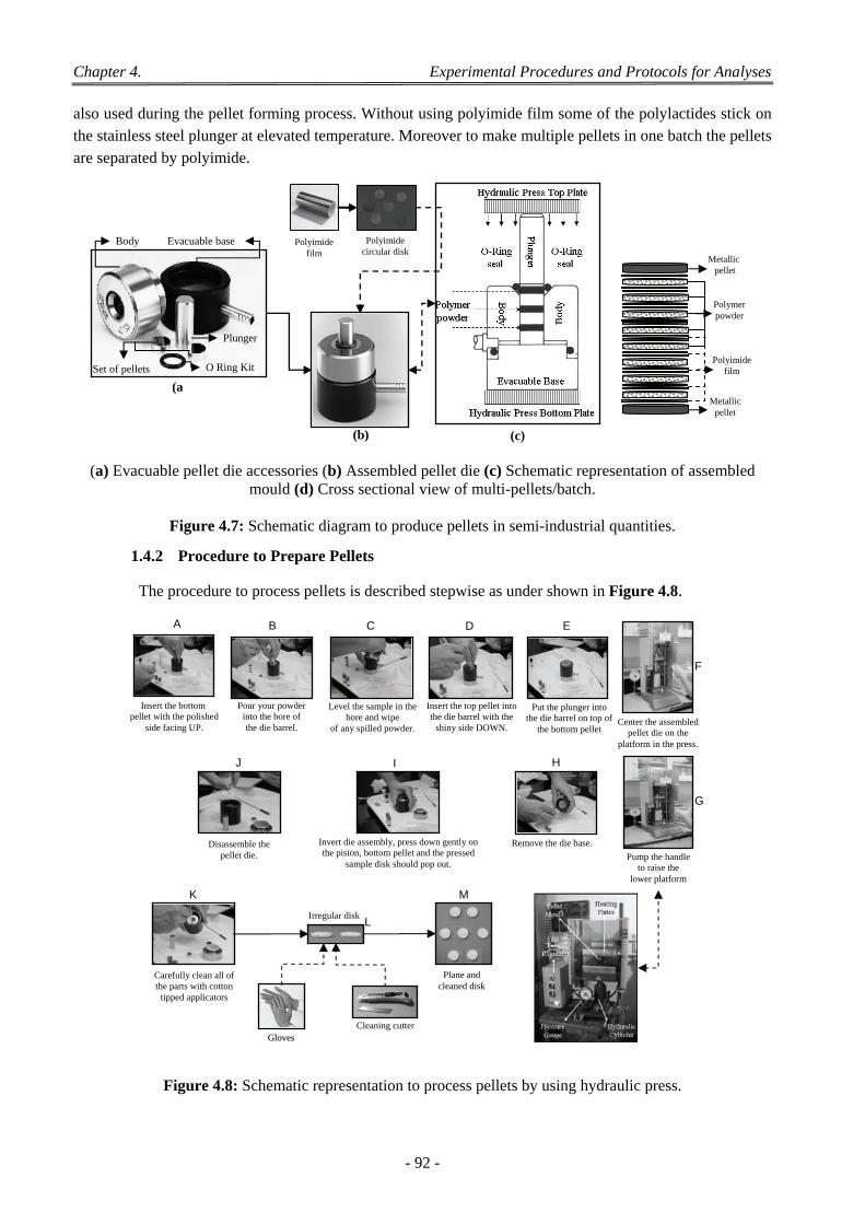
Chapter 4. Experimental Procedures and Protocols for Analyses
- 92 -
also used during the pellet forming process. Without using polyimide film some of the polylactides stick on the stainless steel plunger at elevated temperature. Moreover to make multiple pellets in one batch the pellets
are separated by polyimide.
(a) Evacuable pellet die accessories (b) Assembled pellet die (c) Schematic representation of assembled mould (d) Cross sectional view of multi-pellets/batch.
Figure 4.7: Schematic diagram to produce pellets in semi-industrial quantities.
1.4.2 Procedure to Prepare Pellets
The procedure to process pellets is described stepwise as under shown in Figure 4.8.
Figure 4.8: Schematic representation to process pellets by using hydraulic press.
O Ring Kit Set of pellets
Plunger
Body Evacuable base
(a
(b)
Polyimide film
Polyimide circular disk
(c)
Metallic pellet
Metallicpellet
Polymer powder
Polyimidefilm
Insert the top pellet into the die barrel with the
shiny side DOWN.
Put the plunger into the die barrel on top of
the bottom pellet Center the assembled
pellet die on the platform in the press.
Pump the handle to raise the
lower platform
Insert the bottom pellet with the polished
side facing UP.
Pour your powder into the bore of the die barrel.
B
Level the sample in the bore and wipe
of any spilled powder.
C D E
F
G
Remove the die base.
H
Invert die assembly, press down gently on the piston, bottom pellet and the pressed
sample disk should pop out.
I
GGlloovveess
Disassemble the pellet die.
Carefully clean all of the parts with cotton
tipped applicators
Cleaning cutter
Irregular disk
J
K
L
Plane and cleaned disk
M
A
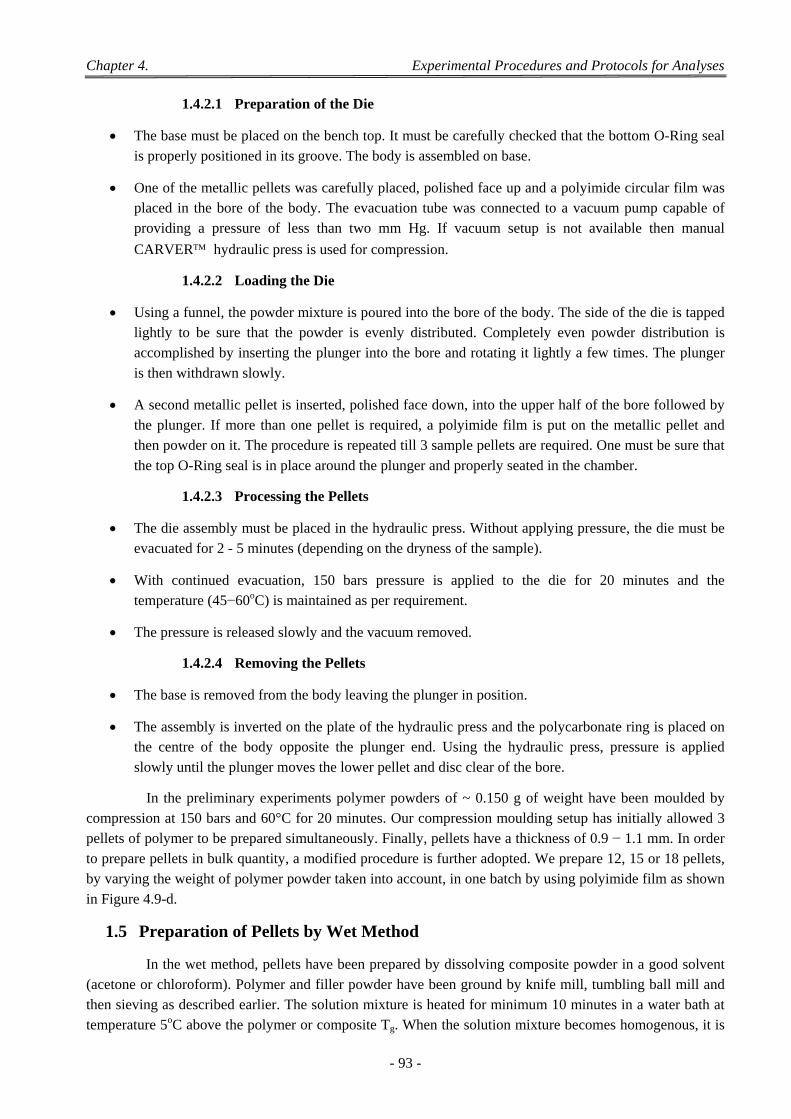
Chapter 4. Experimental Procedures and Protocols for Analyses
- 93 -
1.4.2.1 Preparation of the Die
The base must be placed on the bench top. It must be carefully checked that the bottom O-Ring seal is properly positioned in its groove. The body is assembled on base.
One of the metallic pellets was carefully placed, polished face up and a polyimide circular film was placed in the bore of the body. The evacuation tube was connected to a vacuum pump capable of providing a pressure of less than two mm Hg. If vacuum setup is not available then manual
CARVER hydraulic press is used for compression.
1.4.2.2 Loading the Die
Using a funnel, the powder mixture is poured into the bore of the body. The side of the die is tapped lightly to be sure that the powder is evenly distributed. Completely even powder distribution is accomplished by inserting the plunger into the bore and rotating it lightly a few times. The plunger
is then withdrawn slowly.
A second metallic pellet is inserted, polished face down, into the upper half of the bore followed by the plunger. If more than one pellet is required, a polyimide film is put on the metallic pellet and then powder on it. The procedure is repeated till 3 sample pellets are required. One must be sure that
the top O-Ring seal is in place around the plunger and properly seated in the chamber.
1.4.2.3 Processing the Pellets
The die assembly must be placed in the hydraulic press. Without applying pressure, the die must be evacuated for 2 - 5 minutes (depending on the dryness of the sample).
With continued evacuation, 150 bars pressure is applied to the die for 20 minutes and the temperature (45−60oC) is maintained as per requirement.
The pressure is released slowly and the vacuum removed.
1.4.2.4 Removing the Pellets
The base is removed from the body leaving the plunger in position.
The assembly is inverted on the plate of the hydraulic press and the polycarbonate ring is placed on the centre of the body opposite the plunger end. Using the hydraulic press, pressure is applied
slowly until the plunger moves the lower pellet and disc clear of the bore.
In the preliminary experiments polymer powders of ~ 0.150 g of weight have been moulded by compression at 150 bars and 60°C for 20 minutes. Our compression moulding setup has initially allowed 3 pellets of polymer to be prepared simultaneously. Finally, pellets have a thickness of 0.9 − 1.1 mm. In order to prepare pellets in bulk quantity, a modified procedure is further adopted. We prepare 12, 15 or 18 pellets, by varying the weight of polymer powder taken into account, in one batch by using polyimide film as shown
in Figure 4.9-d.
1.5 Preparation of Pellets by Wet Method
In the wet method, pellets have been prepared by dissolving composite powder in a good solvent (acetone or chloroform). Polymer and filler powder have been ground by knife mill, tumbling ball mill and then sieving as described earlier. The solution mixture is heated for minimum 10 minutes in a water bath at temperature 5oC above the polymer or composite Tg. When the solution mixture becomes homogenous, it is
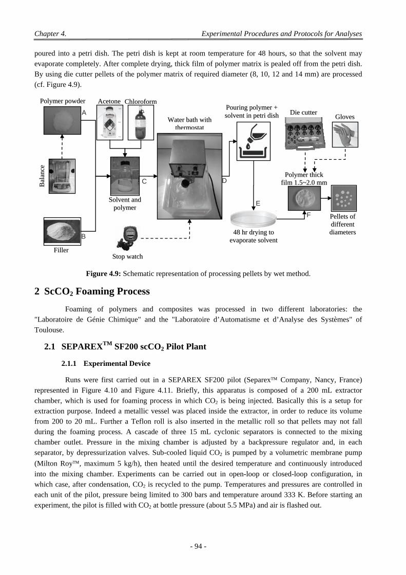
Chapter 4. Experimental Procedures and Protocols for Analyses
- 94 -
poured into a petri dish. The petri dish is kept at room temperature for 48 hours, so that the solvent may evaporate completely. After complete drying, thick film of polymer matrix is pealed off from the petri dish. By using die cutter pellets of the polymer matrix of required diameter (8, 10, 12 and 14 mm) are processed
(cf. Figure 4.9).
Figure 4.9: Schematic representation of processing pellets by wet method.
2 ScCO2 Foaming Process
Foaming of polymers and composites was processed in two different laboratories: the "Laboratoire de Génie Chimique" and the "Laboratoire d’Automatisme et d’Analyse des Systèmes" of
Toulouse.
2.1 SEPAREXTM SF200 scCO2 Pilot Plant
2.1.1 Experimental Device
Runs were first carried out in a SEPAREX SF200 pilot (Separex Company, Nancy, France)
represented in Figure 4.10 and Figure 4.11. Briefly, this apparatus is composed of a 200 mL extractor chamber, which is used for foaming process in which CO2 is being injected. Basically this is a setup for extraction purpose. Indeed a metallic vessel was placed inside the extractor, in order to reduce its volume from 200 to 20 mL. Further a Teflon roll is also inserted in the metallic roll so that pellets may not fall during the foaming process. A cascade of three 15 mL cyclonic separators is connected to the mixing chamber outlet. Pressure in the mixing chamber is adjusted by a backpressure regulator and, in each separator, by depressurization valves. Sub-cooled liquid CO2 is pumped by a volumetric membrane pump
(Milton Roy, maximum 5 kg/h), then heated until the desired temperature and continuously introduced
into the mixing chamber. Experiments can be carried out in open-loop or closed-loop configuration, in which case, after condensation, CO2 is recycled to the pump. Temperatures and pressures are controlled in each unit of the pilot, pressure being limited to 300 bars and temperature around 333 K. Before starting an
experiment, the pilot is filled with CO2 at bottle pressure (about 5.5 MPa) and air is flashed out.
FFiilllleerr SSttoopp wwaattcchh
AAcceettoonnee CChhlloorrooffoorrmm
WWaatteerr bbaatthh wwiitthh tthheerrmmoossttaatt
SSoollvveenntt aanndd ppoollyymmeerr
PPoouurriinngg ppoollyymmeerr ++ ssoollvveenntt iinn ppeettrrii ddiisshh
4488 hhrr ddrryyiinngg ttoo eevvaappoorraattee ssoollvveenntt
PPoollyymmeerr tthhiicckk ffiillmm 11..55~~22..00 mmmm BB
aa llaa nn
cc ee
DDiiee ccuutttteerr
PPeelllleettss ooff ddiiffffeerreenntt ddiiaammeetteerrss
GGlloovveessA
B
C D
E
F
PPoollyymmeerr ppoowwddeerr
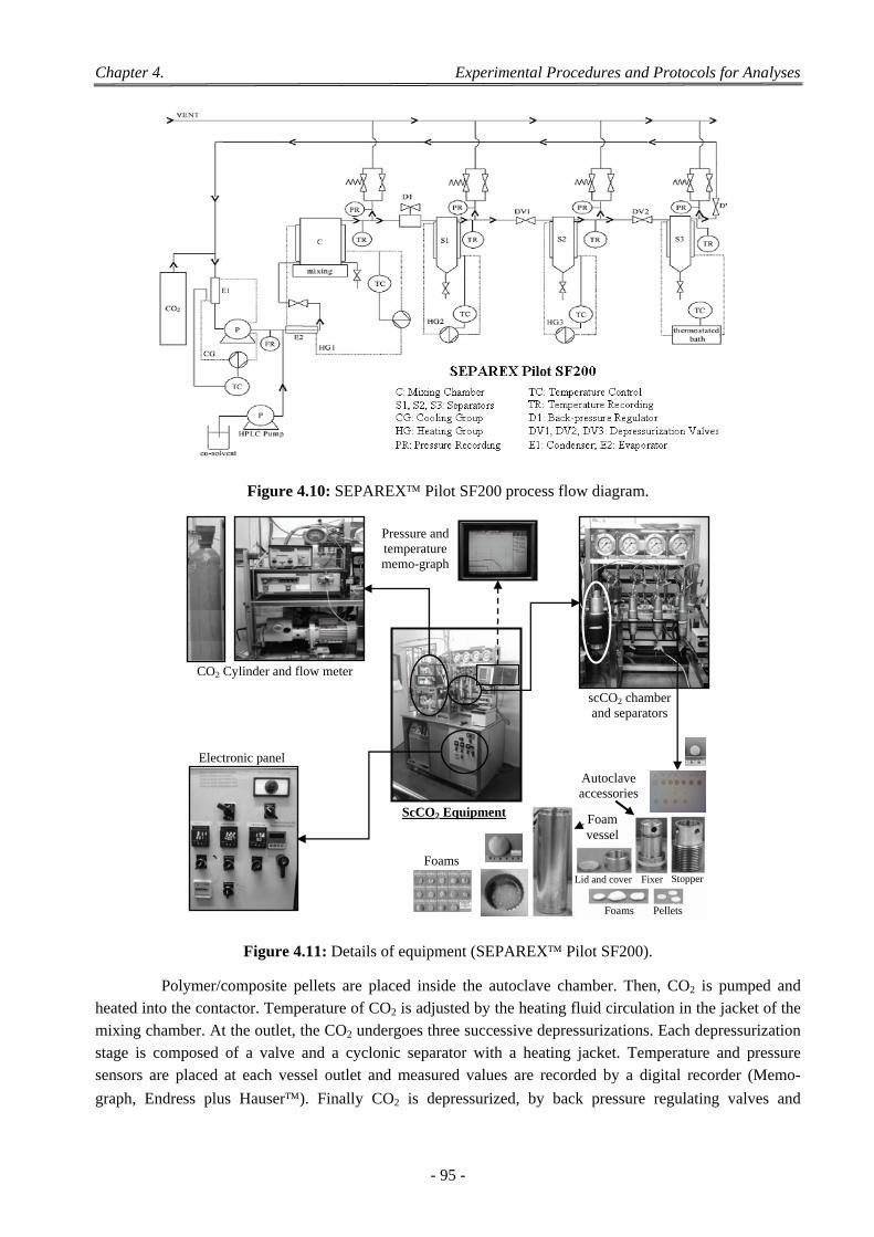
Chapter 4. Experimental Procedures and Protocols for Analyses
- 95 -
Figure 4.10: SEPAREX Pilot SF200 process flow diagram.
Figure 4.11: Details of equipment (SEPAREX Pilot SF200).
Polymer/composite pellets are placed inside the autoclave chamber. Then, CO2 is pumped and heated into the contactor. Temperature of CO2 is adjusted by the heating fluid circulation in the jacket of the mixing chamber. At the outlet, the CO2 undergoes three successive depressurizations. Each depressurization stage is composed of a valve and a cyclonic separator with a heating jacket. Temperature and pressure sensors are placed at each vessel outlet and measured values are recorded by a digital recorder (Memo-
graph, Endress plus Hauser). Finally CO2 is depressurized, by back pressure regulating valves and
Lid and cover Fixer
Foams Pellets
Foam vessel
ScCO2 Equipment
Electronic panel
scCO2 chamber and separators
Pressure and temperature memo-graph
Foams
Autoclave accessories
CO2 Cylinder and flow meter
Stopper
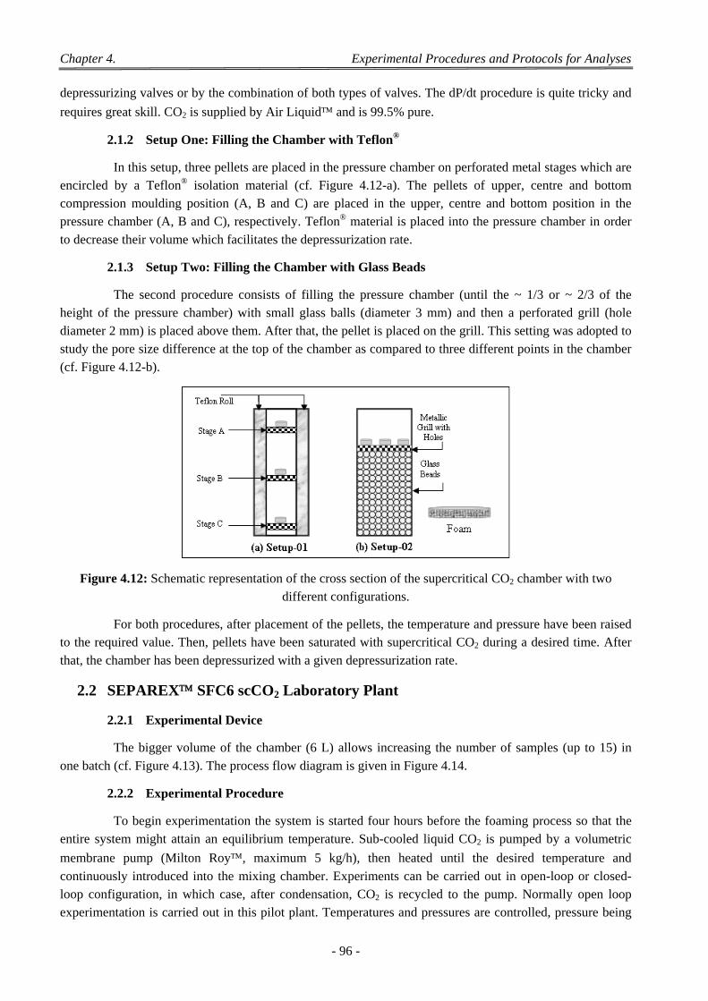
Chapter 4. Experimental Procedures and Protocols for Analyses
- 96 -
depressurizing valves or by the combination of both types of valves. The dP/dt procedure is quite tricky and
requires great skill. CO2 is supplied by Air Liquid and is 99.5% pure.
2.1.2 Setup One: Filling the Chamber with Teflon®
In this setup, three pellets are placed in the pressure chamber on perforated metal stages which are encircled by a Teflon® isolation material (cf. Figure 4.12-a). The pellets of upper, centre and bottom compression moulding position (A, B and C) are placed in the upper, centre and bottom position in the pressure chamber (A, B and C), respectively. Teflon® material is placed into the pressure chamber in order
to decrease their volume which facilitates the depressurization rate.
2.1.3 Setup Two: Filling the Chamber with Glass Beads
The second procedure consists of filling the pressure chamber (until the ~ 1/3 or ~ 2/3 of the height of the pressure chamber) with small glass balls (diameter 3 mm) and then a perforated grill (hole diameter 2 mm) is placed above them. After that, the pellet is placed on the grill. This setting was adopted to study the pore size difference at the top of the chamber as compared to three different points in the chamber
(cf. Figure 4.12-b).
Figure 4.12: Schematic representation of the cross section of the supercritical CO2 chamber with two different configurations.
For both procedures, after placement of the pellets, the temperature and pressure have been raised to the required value. Then, pellets have been saturated with supercritical CO2 during a desired time. After
that, the chamber has been depressurized with a given depressurization rate.
2.2 SEPAREX SFC6 scCO2 Laboratory Plant
2.2.1 Experimental Device
The bigger volume of the chamber (6 L) allows increasing the number of samples (up to 15) in
one batch (cf. Figure 4.13). The process flow diagram is given in Figure 4.14.
2.2.2 Experimental Procedure
To begin experimentation the system is started four hours before the foaming process so that the entire system might attain an equilibrium temperature. Sub-cooled liquid CO2 is pumped by a volumetric
membrane pump (Milton Roy, maximum 5 kg/h), then heated until the desired temperature and
continuously introduced into the mixing chamber. Experiments can be carried out in open-loop or closed-loop configuration, in which case, after condensation, CO2 is recycled to the pump. Normally open loop experimentation is carried out in this pilot plant. Temperatures and pressures are controlled, pressure being
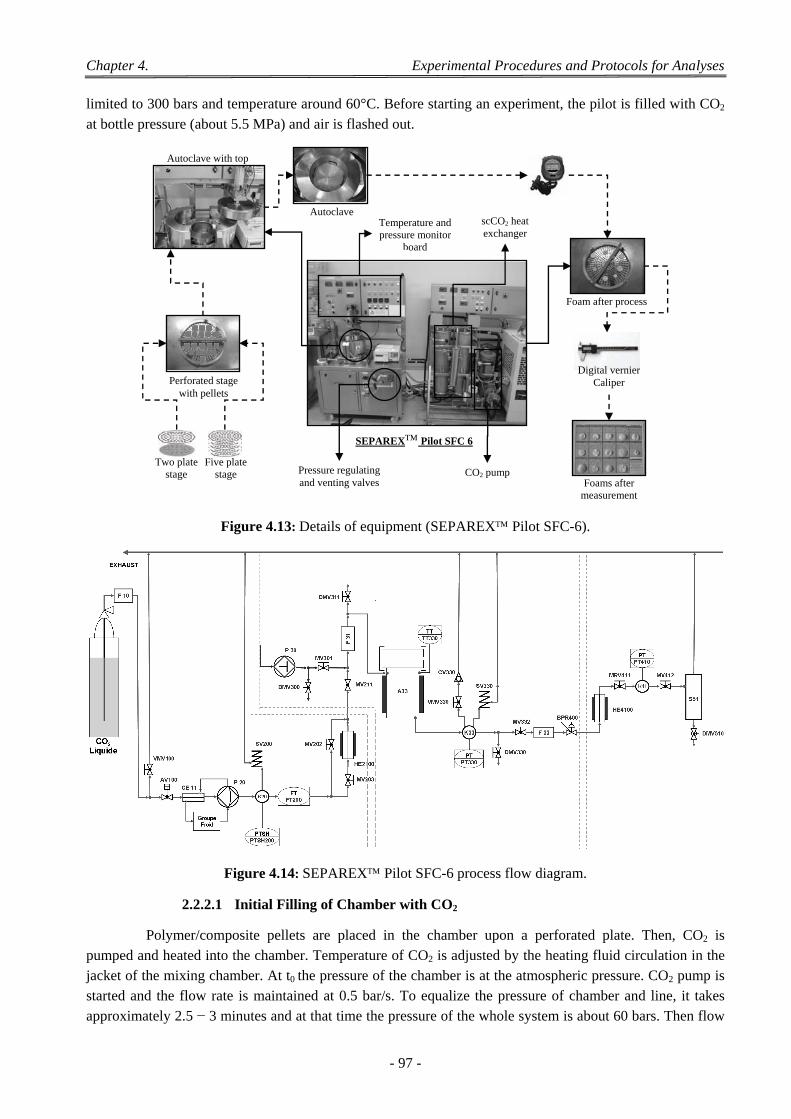
Chapter 4. Experimental Procedures and Protocols for Analyses
- 97 -
limited to 300 bars and temperature around 60°C. Before starting an experiment, the pilot is filled with CO2
at bottle pressure (about 5.5 MPa) and air is flashed out.
Figure 4.13: Details of equipment (SEPAREX Pilot SFC-6).
Figure 4.14: SEPAREX Pilot SFC-6 process flow diagram.
2.2.2.1 Initial Filling of Chamber with CO2
Polymer/composite pellets are placed in the chamber upon a perforated plate. Then, CO2 is pumped and heated into the chamber. Temperature of CO2 is adjusted by the heating fluid circulation in the jacket of the mixing chamber. At t0 the pressure of the chamber is at the atmospheric pressure. CO2 pump is started and the flow rate is maintained at 0.5 bar/s. To equalize the pressure of chamber and line, it takes approximately 2.5 − 3 minutes and at that time the pressure of the whole system is about 60 bars. Then flow
SEPAREX Pilot SFC 6
Autoclave with top
Perforated stage with pellets
Pressure regulating and venting valves
CO2 pump
scCO2 heat exchanger
Temperature and pressure monitor
board
Two plate
stage Five plate
stage
Autoclave
Foam after process
Digital vernier Caliper
Foams after measurement
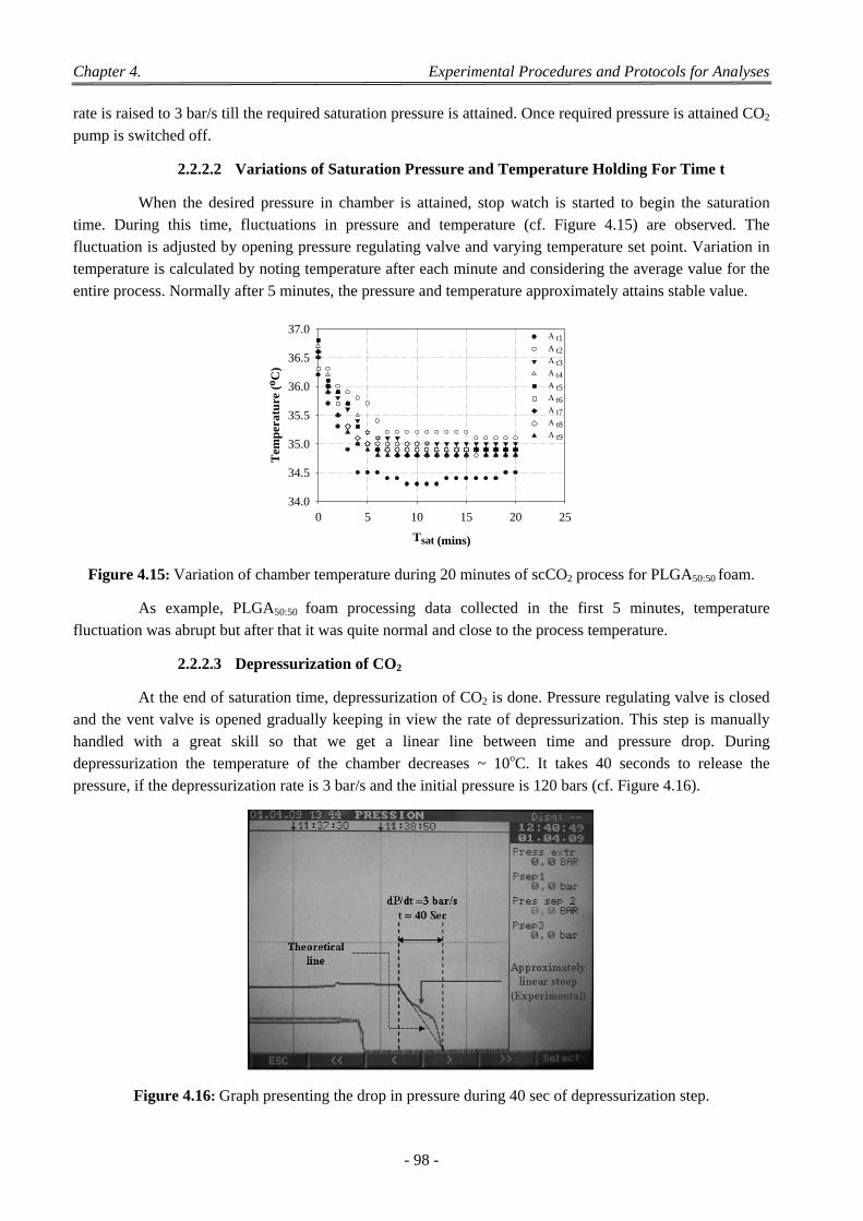
Chapter 4. Experimental Procedures and Protocols for Analyses
- 98 -
rate is raised to 3 bar/s till the required saturation pressure is attained. Once required pressure is attained CO2
pump is switched off.
2.2.2.2 Variations of Saturation Pressure and Temperature Holding For Time t
When the desired pressure in chamber is attained, stop watch is started to begin the saturation time. During this time, fluctuations in pressure and temperature (cf. Figure 4.15) are observed. The fluctuation is adjusted by opening pressure regulating valve and varying temperature set point. Variation in temperature is calculated by noting temperature after each minute and considering the average value for the
entire process. Normally after 5 minutes, the pressure and temperature approximately attains stable value.
Chamber Temperature Variatoion
Tsat (mins)
0 5 10 15 20 25
Tem
per
atu
re (
o C)
34.0
34.5
35.0
35.5
36.0
36.5
37.0A t1A t2A t3A t4A t5A t6A t7A t8A t9
Figure 4.15: Variation of chamber temperature during 20 minutes of scCO2 process for PLGA50:50 foam.
As example, PLGA50:50 foam processing data collected in the first 5 minutes, temperature
fluctuation was abrupt but after that it was quite normal and close to the process temperature.
2.2.2.3 Depressurization of CO2
At the end of saturation time, depressurization of CO2 is done. Pressure regulating valve is closed and the vent valve is opened gradually keeping in view the rate of depressurization. This step is manually handled with a great skill so that we get a linear line between time and pressure drop. During depressurization the temperature of the chamber decreases ~ 10oC. It takes 40 seconds to release the
pressure, if the depressurization rate is 3 bar/s and the initial pressure is 120 bars (cf. Figure 4.16).
Figure 4.16: Graph presenting the drop in pressure during 40 sec of depressurization step.
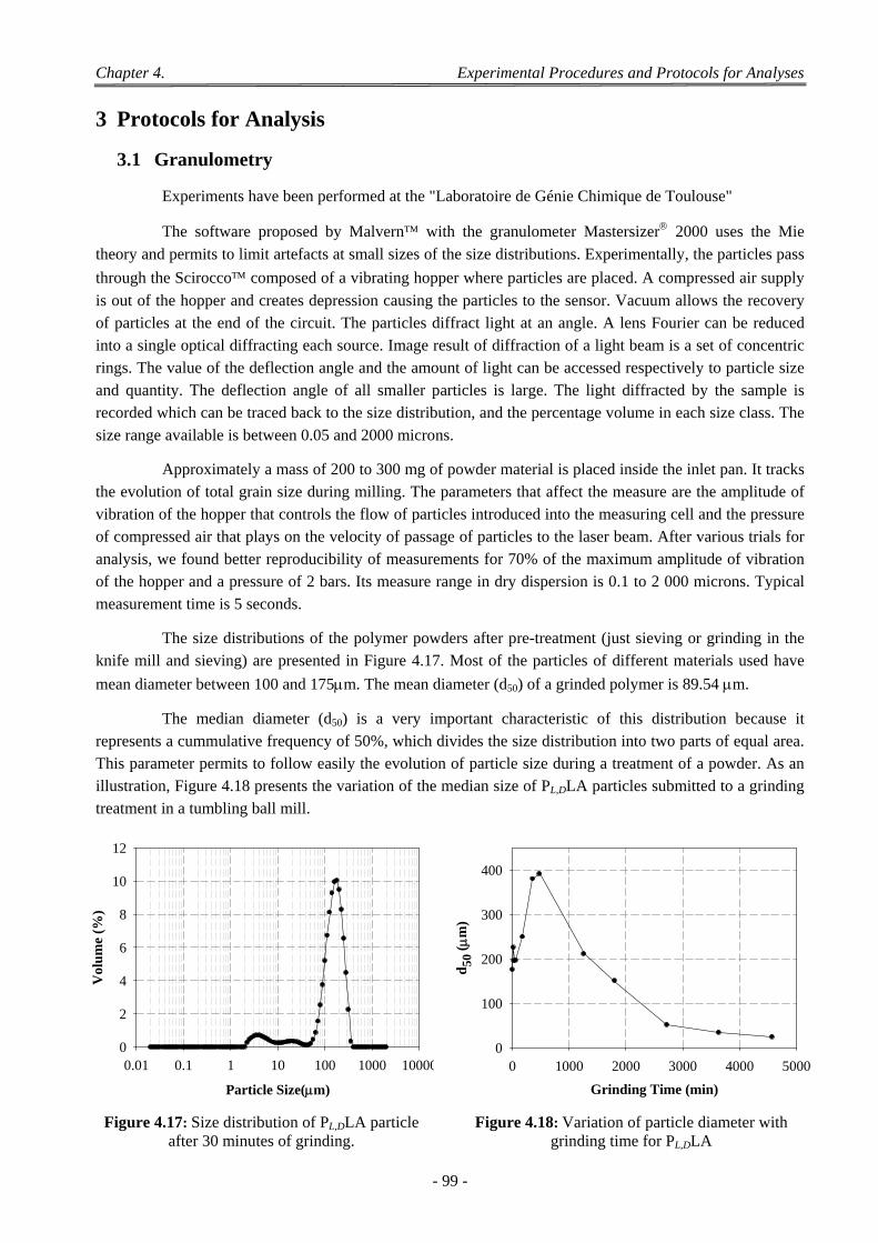
Chapter 4. Experimental Procedures and Protocols for Analyses
- 99 -
3 Protocols for Analysis
3.1 Granulometry
Experiments have been performed at the "Laboratoire de Génie Chimique de Toulouse"
The software proposed by Malvern with the granulometer Mastersizer 2000 uses the Mie
theory and permits to limit artefacts at small sizes of the size distributions. Experimentally, the particles pass
through the Scirocco composed of a vibrating hopper where particles are placed. A compressed air supply
is out of the hopper and creates depression causing the particles to the sensor. Vacuum allows the recovery of particles at the end of the circuit. The particles diffract light at an angle. A lens Fourier can be reduced into a single optical diffracting each source. Image result of diffraction of a light beam is a set of concentric rings. The value of the deflection angle and the amount of light can be accessed respectively to particle size and quantity. The deflection angle of all smaller particles is large. The light diffracted by the sample is recorded which can be traced back to the size distribution, and the percentage volume in each size class. The
size range available is between 0.05 and 2000 microns.
Approximately a mass of 200 to 300 mg of powder material is placed inside the inlet pan. It tracks the evolution of total grain size during milling. The parameters that affect the measure are the amplitude of vibration of the hopper that controls the flow of particles introduced into the measuring cell and the pressure of compressed air that plays on the velocity of passage of particles to the laser beam. After various trials for analysis, we found better reproducibility of measurements for 70% of the maximum amplitude of vibration of the hopper and a pressure of 2 bars. Its measure range in dry dispersion is 0.1 to 2 000 microns. Typical
measurement time is 5 seconds.
The size distributions of the polymer powders after pre-treatment (just sieving or grinding in the knife mill and sieving) are presented in Figure 4.17. Most of the particles of different materials used have
mean diameter between 100 and 175m. The mean diameter (d50) of a grinded polymer is 89.54 m.
The median diameter (d50) is a very important characteristic of this distribution because it represents a cummulative frequency of 50%, which divides the size distribution into two parts of equal area. This parameter permits to follow easily the evolution of particle size during a treatment of a powder. As an illustration, Figure 4.18 presents the variation of the median size of PL,DLA particles submitted to a grinding
treatment in a tumbling ball mill.
Poly (Lactide-co-glycolide) : Granulometry
Particle Size(m)
0.01 0.1 1 10 100 1000 10000
Vol
um
e (%
)
0
2
4
6
8
10
12
Particle Diameter Variation with Grinding time
Grinding Time (min)
0 1000 2000 3000 4000 5000
d50
( m
)
0
100
200
300
400
Figure 4.17: Size distribution of PL,DLA particle after 30 minutes of grinding.
Figure 4.18: Variation of particle diameter with grinding time for PL,DLA
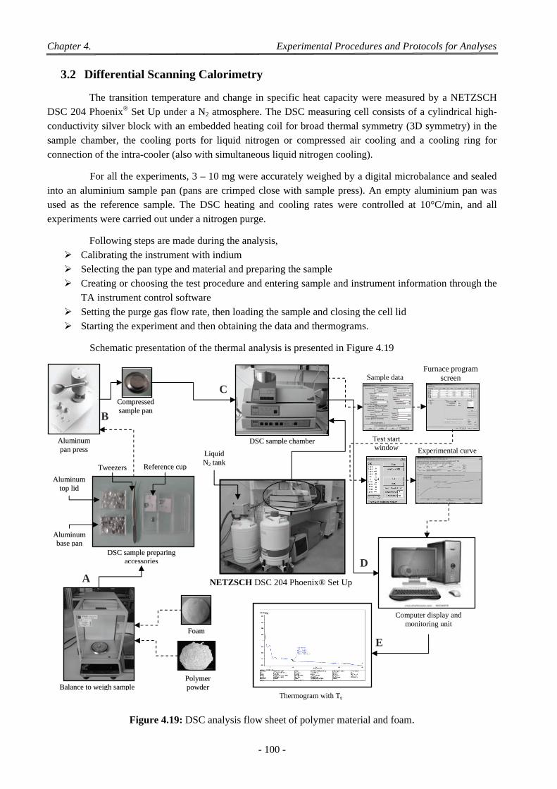
Chapter 4. Experimental Procedures and Protocols for Analyses
- 100 -
3.2 Differential Scanning Calorimetry
The transition temperature and change in specific heat capacity were measured by a NETZSCH DSC 204 Phoenix® Set Up under a N2 atmosphere. The DSC measuring cell consists of a cylindrical high-conductivity silver block with an embedded heating coil for broad thermal symmetry (3D symmetry) in the sample chamber, the cooling ports for liquid nitrogen or compressed air cooling and a cooling ring for
connection of the intra-cooler (also with simultaneous liquid nitrogen cooling).
For all the experiments, 3 – 10 mg were accurately weighed by a digital microbalance and sealed into an aluminium sample pan (pans are crimped close with sample press). An empty aluminium pan was used as the reference sample. The DSC heating and cooling rates were controlled at 10°C/min, and all
experiments were carried out under a nitrogen purge.
Following steps are made during the analysis, Calibrating the instrument with indium Selecting the pan type and material and preparing the sample Creating or choosing the test procedure and entering sample and instrument information through the
TA instrument control software Setting the purge gas flow rate, then loading the sample and closing the cell lid Starting the experiment and then obtaining the data and thermograms.
Schematic presentation of the thermal analysis is presented in Figure 4.19
Figure 4.19: DSC analysis flow sheet of polymer material and foam.
PPoollyymmeerr ppoowwddeerr
DDSSCC ssaammppllee cchhaammbbeerr
BBaallaannccee ttoo wweeiigghh ssaammppllee
FFooaamm
NETZSCH DSC 204 Phoenix® Set Up
DDSSCC ssaammppllee pprreeppaarriinngg aacccceessssoorriieess
AAlluummiinnuumm ttoopp lliidd
AAlluummiinnuumm bbaassee ppaann
TTwweeeezzeerrss RReeffeerreennccee ccuupp
AAlluummiinnuumm ppaann pprreessss
CCoommpprreesssseedd ssaammppllee ppaann
LLiiqquuiidd NN22 ttaannkk
Sample data
Test start window Experimental curve
Computer display and monitoring unit
Thermogram with Tg
A
B
C
D
E
Furnace program screen
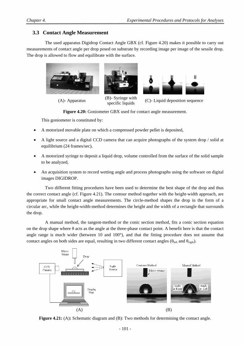
Chapter 4. Experimental Procedures and Protocols for Analyses
- 101 -
3.3 Contact Angle Measurement
The used apparatus Digidrop Contact Angle GBX (cf. Figure 4.20) makes it possible to carry out measurements of contact angle per drop posed on substrate by recording image per image of the sessile drop.
The drop is allowed to flow and equilibrate with the surface.
(A)- Apparatus (B)- Syringe with specific liquids
(C)- Liquid deposition sequence
Figure 4.20: Goniometer GBX used for contact angle measurement.
This goniometer is constituted by:
A motorized movable plate on which a compressed powder pellet is deposited,
A light source and a digital CCD camera that can acquire photographs of the system drop / solid at equilibrium (24 frames/sec),
A motorized syringe to deposit a liquid drop, volume controlled from the surface of the solid sample
to be analyzed,
An acquisition system to record wetting angle and process photographs using the software on digital images DIGIDROP.
Two different fitting procedures have been used to determine the best shape of the drop and thus the correct contact angle (cf. Figure 4.21). The contour method together with the height-width approach, are appropriate for small contact angle measurements. The circle-method shapes the drop in the form of a circular arc, while the height-width-method determines the height and the width of a rectangle that surrounds
the drop.
A manual method, the tangent-method or the conic section method, fits a conic section equation on the drop shape where θ acts as the angle at the three-phase contact point. A benefit here is that the contact angle range is much wider (between 10 and 100°), and that the fitting procedure does not assume that
contact angles on both sides are equal, resulting in two different contact angles (θleft and θrigth).
(A) (B)
Figure 4.21: (A): Schematic diagram and (B): Two methods for determining the contact angle.
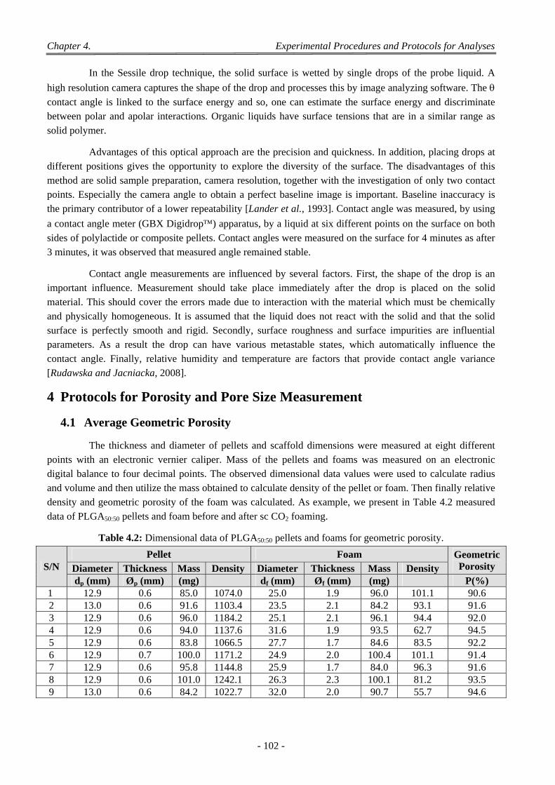
Chapter 4. Experimental Procedures and Protocols for Analyses
- 102 -
In the Sessile drop technique, the solid surface is wetted by single drops of the probe liquid. A
high resolution camera captures the shape of the drop and processes this by image analyzing software. The
contact angle is linked to the surface energy and so, one can estimate the surface energy and discriminate between polar and apolar interactions. Organic liquids have surface tensions that are in a similar range as
solid polymer.
Advantages of this optical approach are the precision and quickness. In addition, placing drops at different positions gives the opportunity to explore the diversity of the surface. The disadvantages of this method are solid sample preparation, camera resolution, together with the investigation of only two contact points. Especially the camera angle to obtain a perfect baseline image is important. Baseline inaccuracy is the primary contributor of a lower repeatability [Lander et al., 1993]. Contact angle was measured, by using
a contact angle meter (GBX Digidrop) apparatus, by a liquid at six different points on the surface on both
sides of polylactide or composite pellets. Contact angles were measured on the surface for 4 minutes as after
3 minutes, it was observed that measured angle remained stable.
Contact angle measurements are influenced by several factors. First, the shape of the drop is an important influence. Measurement should take place immediately after the drop is placed on the solid material. This should cover the errors made due to interaction with the material which must be chemically and physically homogeneous. It is assumed that the liquid does not react with the solid and that the solid surface is perfectly smooth and rigid. Secondly, surface roughness and surface impurities are influential parameters. As a result the drop can have various metastable states, which automatically influence the contact angle. Finally, relative humidity and temperature are factors that provide contact angle variance
[Rudawska and Jacniacka, 2008].
4 Protocols for Porosity and Pore Size Measurement
4.1 Average Geometric Porosity
The thickness and diameter of pellets and scaffold dimensions were measured at eight different points with an electronic vernier caliper. Mass of the pellets and foams was measured on an electronic digital balance to four decimal points. The observed dimensional data values were used to calculate radius and volume and then utilize the mass obtained to calculate density of the pellet or foam. Then finally relative density and geometric porosity of the foam was calculated. As example, we present in Table 4.2 measured
data of PLGA50:50 pellets and foam before and after sc CO2 foaming.
Table 4.2: Dimensional data of PLGA50:50 pellets and foams for geometric porosity.
S/N Pellet Foam Geometric
Porosity Diameter Thickness Mass Density Diameter Thickness Mass Density dp (mm) Øp (mm) (mg) df (mm) Øf (mm) (mg) P(%)
1 12.9 0.6 85.0 1074.0 25.0 1.9 96.0 101.1 90.6 2 13.0 0.6 91.6 1103.4 23.5 2.1 84.2 93.1 91.6 3 12.9 0.6 96.0 1184.2 25.1 2.1 96.1 94.4 92.0 4 12.9 0.6 94.0 1137.6 31.6 1.9 93.5 62.7 94.5 5 12.9 0.6 83.8 1066.5 27.7 1.7 84.6 83.5 92.2 6 12.9 0.7 100.0 1171.2 24.9 2.0 100.4 101.1 91.4 7 12.9 0.6 95.8 1144.8 25.9 1.7 84.0 96.3 91.6 8 12.9 0.6 101.0 1242.1 26.3 2.3 100.1 81.2 93.5 9 13.0 0.6 84.2 1022.7 32.0 2.0 90.7 55.7 94.6
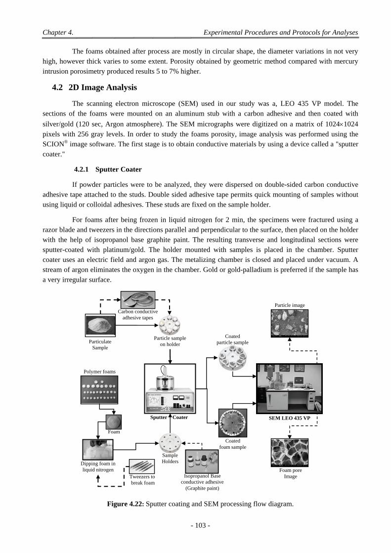
Chapter 4. Experimental Procedures and Protocols for Analyses
- 103 -
The foams obtained after process are mostly in circular shape, the diameter variations in not very high, however thick varies to some extent. Porosity obtained by geometric method compared with mercury
intrusion porosimetry produced results 5 to 7% higher.
4.2 2D Image Analysis
The scanning electron microscope (SEM) used in our study was a, LEO 435 VP model. The sections of the foams were mounted on an aluminum stub with a carbon adhesive and then coated with
silver/gold (120 sec, Argon atmosphere). The SEM micrographs were digitized on a matrix of 10241024
pixels with 256 gray levels. In order to study the foams porosity, image analysis was performed using the SCION® image software. The first stage is to obtain conductive materials by using a device called a "sputter
coater."
4.2.1 Sputter Coater
If powder particles were to be analyzed, they were dispersed on double-sided carbon conductive adhesive tape attached to the studs. Double sided adhesive tape permits quick mounting of samples without
using liquid or colloidal adhesives. These studs are fixed on the sample holder.
For foams after being frozen in liquid nitrogen for 2 min, the specimens were fractured using a razor blade and tweezers in the directions parallel and perpendicular to the surface, then placed on the holder with the help of isopropanol base graphite paint. The resulting transverse and longitudinal sections were sputter-coated with platinum/gold. The holder mounted with samples is placed in the chamber. Sputter coater uses an electric field and argon gas. The metalizing chamber is closed and placed under vacuum. A stream of argon eliminates the oxygen in the chamber. Gold or gold-palladium is preferred if the sample has
a very irregular surface.
Figure 4.22: Sputter coating and SEM processing flow diagram.
Particulate Sample
Particle sample on holder
Carbon conductive adhesive tapes
Particle image
Polymer foams
Tweezers to break foam
Dipping foam in liquid nitrogen
Sample Holders
Foam
Coated foam sample
Coated particle sample
Foam pore Image
SEM LEO 435 VP Sputter Coater
Isopropanol Base conductive adhesive
(Graphite paint)
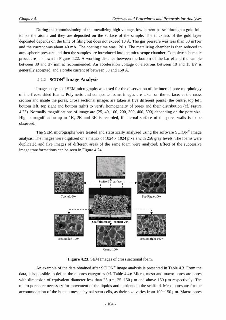
Chapter 4. Experimental Procedures and Protocols for Analyses
- 104 -
During the commissioning of the metalizing high voltage, low current passes through a gold foil, ionize the atoms and they are deposited on the surface of the sample. The thickness of the gold layer deposited depends on the time of filing but does not exceed 10 Å. The gas pressure was less than 50 mTorr and the current was about 40 mA. The coating time was 120 s. The metalizing chamber is then reduced to atmospheric pressure and then the samples are introduced into the microscope chamber. Complete schematic procedure is shown in Figure 4.22. A working distance between the bottom of the barrel and the sample between 30 and 37 mm is recommended. An acceleration voltage of electrons between 10 and 15 kV is
generally accepted, and a probe current of between 50 and 150 Å.
4.2.2 SCION Image Analysis
Image analysis of SEM micrographs was used for the observation of the internal pore morphology of the freeze-dried foams. Polymeric and composite foams images are taken on the surface, at the cross section and inside the pores. Cross sectional images are taken at five different points (the centre, top left, bottom left, top right and bottom right) to verify homogeneity of pores and their distribution (cf. Figure 4.23). Normally magnifications of image are (25, 40, 100, 200, 300, 400, 500) depending on the pore size. Higher magnification up to 1K, 2K and 3K is recorded, if internal surface of the pores walls is to be
observed.
The SEM micrographs were treated and statistically analyzed using the software SCION® Image
analysis. The images were digitized on a matrix of 1024 1024 pixels with 256 gray levels. The foams were
duplicated and five images of different areas of the same foam were analyzed. Effect of the successive
image transformations can be seen in Figure 4.24.
Figure 4.23: SEM Images of cross sectional foam.
An example of the data obtained after SCION® image analysis is presented in Table 4.3. From the data, it is possible to define three pores categories (cf. Table 4.4): Micro, meso and macro pores are pores
with dimension of equivalent diameter less than 25 m, 25−150 m and above 150 m respectively. The
micro pores are necessary for movement of the liquids and nutrients in the scaffold. Meso pores are for the
accommodation of the human mesenchymal stem cells, as their size varies from 100−150 m. Macro pores
Bottom left-100×
Top Right-100×
Scaffold surface
Top left-50×
Scaffold cross- section-20×
Bottom right-100×
Centre-100×
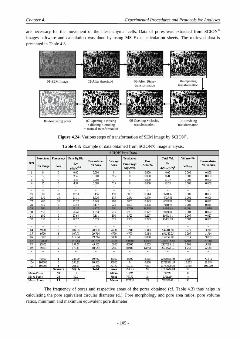
Chapter 4. Experimental Procedures and Protocols for Analyses
- 105 -
are necessary for the movement of the mesenchymal cells. Data of pores was extracted from SCION® images software and calculation was done by using MS Excel calculation sheets. The retrieved data is
presented in Table 4.3.
Figure 4.24: Various steps of transformation of SEM image by SCION®.
Table 4.3: Example of data obtained from SCION® image analysis.
The frequency of pores and respective areas of the pores obtained (cf. Table 4.3) thus helps in calculating the pore equivalent circular diameter (de). Pore morphology and pore area ratios, pore volume
ratios, minimum and maximum equivalent pore diameter.
02-After threshold 03-After Binary transformation
04-Opening transformation
05-Erodeing transformation
06-Opening + closing transformation
07-Opening + closing + dilating + eroding
+ manual transformation
08-Analyzing pores
01-SEM Image
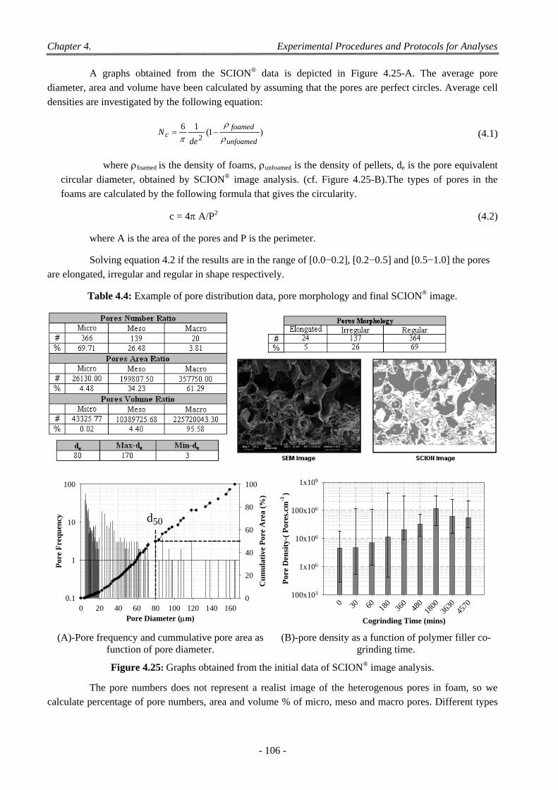
Chapter 4. Experimental Procedures and Protocols for Analyses
- 106 -
A graphs obtained from the SCION® data is depicted in Figure 4.25-A. The average pore diameter, area and volume have been calculated by assuming that the pores are perfect circles. Average cell
densities are investigated by the following equation:
)1(16
2 unfoamed
foamedc
deN
(4.1)
where foamed is the density of foams, unfoamed is the density of pellets, de is the pore equivalent
circular diameter, obtained by SCION® image analysis. (cf. Figure 4.25-B).The types of pores in the
foams are calculated by the following formula that gives the circularity.
c = 4 A/P2 (4.2)
where A is the area of the pores and P is the perimeter.
Solving equation 4.2 if the results are in the range of [0.0−0.2], [0.2−0.5] and [0.5−1.0] the pores
are elongated, irregular and regular in shape respectively.
Table 4.4: Example of pore distribution data, pore morphology and final SCION® image.
2D Graph 2
Pore Diameter (m)0 20 40 60 80 100 120 140 160
Por
e F
req
uen
cy
0.1
1
10
100
Cu
mu
lati
ve P
ore
Are
a (%
)
0
20
40
60
80
100
d50
Pore Density : Taguchi Plan-I
Cogrinding Time (mins)
0 30 60 180
360
480
1800
3630
4570
Por
e D
ensi
ty-(
Por
es.c
m-3
)
100x103
1x10⁶
10x106
100x106
1x10⁹
(A)-Pore frequency and cummulative pore area as function of pore diameter.
(B)-pore density as a function of polymer filler co-grinding time.
Figure 4.25: Graphs obtained from the initial data of SCION® image analysis.
The pore numbers does not represent a realist image of the heterogenous pores in foam, so we calculate percentage of pore numbers, area and volume % of micro, meso and macro pores. Different types
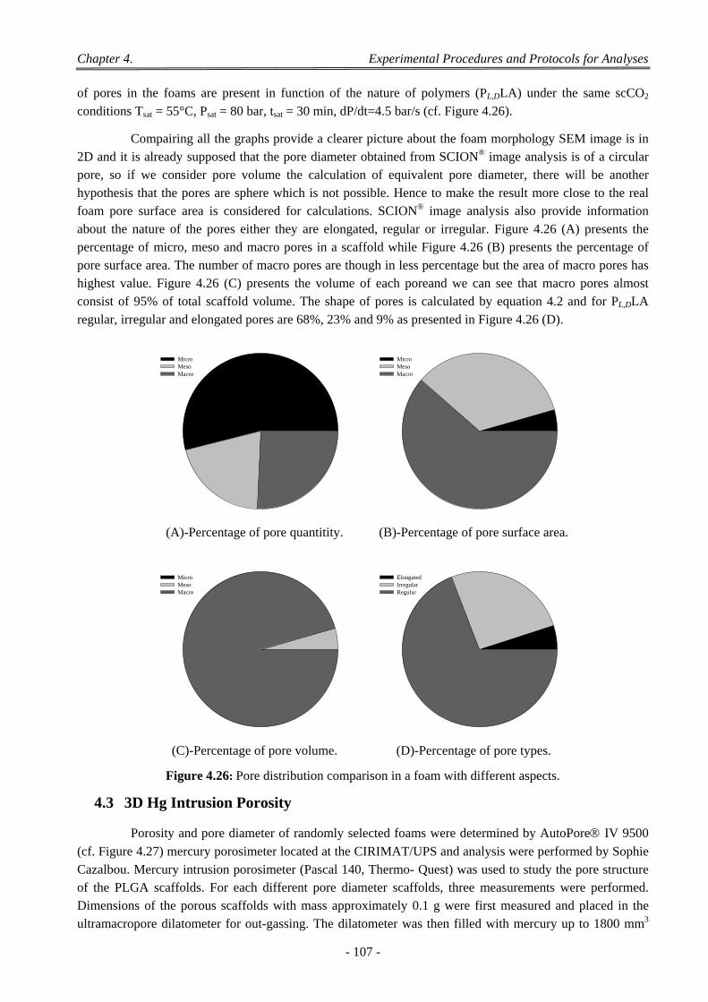
Chapter 4. Experimental Procedures and Protocols for Analyses
- 107 -
of pores in the foams are present in function of the nature of polymers (PL,DLA) under the same scCO2
conditions Tsat = 55°C, Psat = 80 bar, tsat = 30 min, dP/dt=4.5 bar/s (cf. Figure 4.26).
Compairing all the graphs provide a clearer picture about the foam morphology SEM image is in 2D and it is already supposed that the pore diameter obtained from SCION® image analysis is of a circular pore, so if we consider pore volume the calculation of equivalent pore diameter, there will be another hypothesis that the pores are sphere which is not possible. Hence to make the result more close to the real foam pore surface area is considered for calculations. SCION® image analysis also provide information about the nature of the pores either they are elongated, regular or irregular. Figure 4.26 (A) presents the percentage of micro, meso and macro pores in a scaffold while Figure 4.26 (B) presents the percentage of pore surface area. The number of macro pores are though in less percentage but the area of macro pores has highest value. Figure 4.26 (C) presents the volume of each poreand we can see that macro pores almost consist of 95% of total scaffold volume. The shape of pores is calculated by equation 4.2 and for PL,DLA
regular, irregular and elongated pores are 68%, 23% and 9% as presented in Figure 4.26 (D).
Pie Graph 1
MicroMesoMacro
Pie Graph 1
MicroMesoMacro
(A)-Percentage of pore quantitity. (B)-Percentage of pore surface area.
Pie Graph 1
MicroMesoMacro
Pie Graph 1
ElongatedIrregularRegular
(C)-Percentage of pore volume. (D)-Percentage of pore types.
Figure 4.26: Pore distribution comparison in a foam with different aspects.
4.3 3D Hg Intrusion Porosity
Porosity and pore diameter of randomly selected foams were determined by AutoPore IV 9500
(cf. Figure 4.27) mercury porosimeter located at the CIRIMAT/UPS and analysis were performed by Sophie Cazalbou. Mercury intrusion porosimeter (Pascal 140, Thermo- Quest) was used to study the pore structure of the PLGA scaffolds. For each different pore diameter scaffolds, three measurements were performed. Dimensions of the porous scaffolds with mass approximately 0.1 g were first measured and placed in the ultramacropore dilatometer for out-gassing. The dilatometer was then filled with mercury up to 1800 mm3
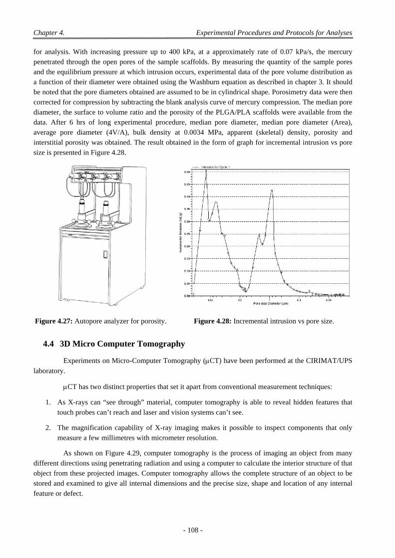
Chapter 4. Experimental Procedures and Protocols for Analyses
- 108 -
for analysis. With increasing pressure up to 400 kPa, at a approximately rate of 0.07 kPa/s, the mercury penetrated through the open pores of the sample scaffolds. By measuring the quantity of the sample pores and the equilibrium pressure at which intrusion occurs, experimental data of the pore volume distribution as a function of their diameter were obtained using the Washburn equation as described in chapter 3. It should be noted that the pore diameters obtained are assumed to be in cylindrical shape. Porosimetry data were then corrected for compression by subtracting the blank analysis curve of mercury compression. The median pore diameter, the surface to volume ratio and the porosity of the PLGA/PLA scaffolds were available from the data. After 6 hrs of long experimental procedure, median pore diameter, median pore diameter (Area), average pore diameter (4V/A), bulk density at 0.0034 MPa, apparent (skeletal) density, porosity and interstitial porosity was obtained. The result obtained in the form of graph for incremental intrusion vs pore
size is presented in Figure 4.28.
Figure 4.27: Autopore analyzer for porosity. Figure 4.28: Incremental intrusion vs pore size.
4.4 3D Micro Computer Tomography
Experiments on Micro-Computer Tomography (CT) have been performed at the CIRIMAT/UPS
laboratory.
CT has two distinct properties that set it apart from conventional measurement techniques:
1. As X-rays can “see through” material, computer tomography is able to reveal hidden features that
touch probes can’t reach and laser and vision systems can’t see.
2. The magnification capability of X-ray imaging makes it possible to inspect components that only
measure a few millimetres with micrometer resolution.
As shown on Figure 4.29, computer tomography is the process of imaging an object from many different directions using penetrating radiation and using a computer to calculate the interior structure of that object from these projected images. Computer tomography allows the complete structure of an object to be stored and examined to give all internal dimensions and the precise size, shape and location of any internal
feature or defect.

Chapter 4. Experimental Procedures and Protocols for Analyses
- 109 -
Figure 4.29: Set up of CT and flow chart of CT measurement process.
4.4.1 Acquisition
The sample is rotated through 360 degrees on a precision turntable and a set of high resolution digital radiographs are acquired at regular (typically 0.5 degree) increments. The accuracy of this data set
determines the ultimate quality of the final 3D data.
4.4.2 Corrections
Each projected image from the data set undergoes geometric and shading correction, to remove
spatial and intensity non linearities introduced by the imaging device.
4.4.3 Reconstruction
By combining all of the individually corrected images and using a cone beam back projection technique, a geometrically correct, three dimensional data cloud is computed. The patented software has a
real-time viewer that shows the reconstruction progressing in parallel with the x-ray images being captured.
4.4.4 Viewing Results
The CT data collection, reconstruction and display are presented to the operator via the X-Tek graphical user interface. This has been developed to provide ease of use with the highest performance for systems to fit users’ budgets without compromise. The data cloud can be sliced open in any direction to reveal internal detail, surface rendering software similar to that used in 3D CAD systems is used to visualise
the exposed features.
4.4.5 Wide Variety of Post Processing
The data cloud can be output as a stereo lithography file, a format accepted by most CAD packages. Once imported into a CAD system, the radiographic information can be compared directly with the original design file to highlight differences when checking first off manufactured parts, or if the original design is not available, then the radiographic data is used to create a new CAD file for rapid prototyping and
reverse engineering.
Micro CT of different scaffolds was taken from different angles and views. Slices were taken to observe the interconnectivity and porosity of the scaffold structure. An example of a polymer skeletal structure along the top, front and right views are taken (cf. Figure 4.30). These images can be further used
for porosity and pore size distribution analysis. CT can directly provide the porosity and interconnectivity
in tested foam. The results obtained from CT are real results compared to the results obtained from
calculations and other derived analysis such as images analysis.
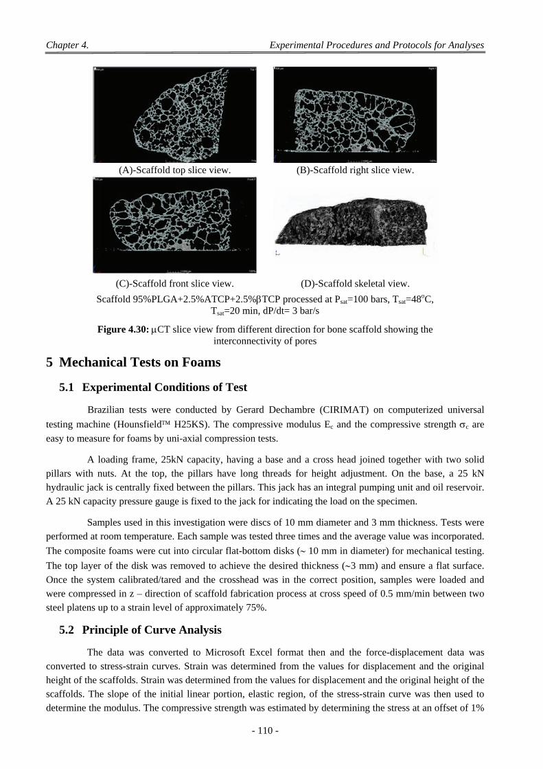
Chapter 4. Experimental Procedures and Protocols for Analyses
- 110 -
(A)-Scaffold top slice view. (B)-Scaffold right slice view.
(C)-Scaffold front slice view. (D)-Scaffold skeletal view.
Scaffold 95%PLGA+2.5%ATCP+2.5%TCP processed at Psat=100 bars, Tsat=48oC, Tsat=20 min, dP/dt= 3 bar/s
Figure 4.30: CT slice view from different direction for bone scaffold showing the interconnectivity of pores
5 Mechanical Tests on Foams
5.1 Experimental Conditions of Test
Brazilian tests were conducted by Gerard Dechambre (CIRIMAT) on computerized universal
testing machine (Hounsfield H25KS). The compressive modulus Ec and the compressive strength c are
easy to measure for foams by uni-axial compression tests.
A loading frame, 25kN capacity, having a base and a cross head joined together with two solid pillars with nuts. At the top, the pillars have long threads for height adjustment. On the base, a 25 kN hydraulic jack is centrally fixed between the pillars. This jack has an integral pumping unit and oil reservoir.
A 25 kN capacity pressure gauge is fixed to the jack for indicating the load on the specimen.
Samples used in this investigation were discs of 10 mm diameter and 3 mm thickness. Tests were performed at room temperature. Each sample was tested three times and the average value was incorporated.
The composite foams were cut into circular flat-bottom disks (10 mm in diameter) for mechanical testing.
The top layer of the disk was removed to achieve the desired thickness (3 mm) and ensure a flat surface.
Once the system calibrated/tared and the crosshead was in the correct position, samples were loaded and were compressed in z – direction of scaffold fabrication process at cross speed of 0.5 mm/min between two steel platens up to a strain level of approximately 75%.
5.2 Principle of Curve Analysis
The data was converted to Microsoft Excel format then and the force-displacement data was converted to stress-strain curves. Strain was determined from the values for displacement and the original height of the scaffolds. Strain was determined from the values for displacement and the original height of the scaffolds. The slope of the initial linear portion, elastic region, of the stress-strain curve was then used to determine the modulus. The compressive strength was estimated by determining the stress at an offset of 1%
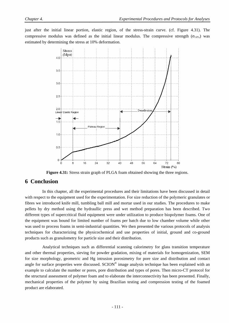
Chapter 4. Experimental Procedures and Protocols for Analyses
- 111 -
just after the initial linear portion, elastic region, of the stress-strain curve. (cf. Figure 4.31). The
compressive modulus was defined as the initial linear modulus. The compressive strength () was
estimated by determining the stress at 10% deformation.
Figure 4.31: Stress strain graph of PLGA foam obtained showing the three regions.
6 Conclusion
In this chapter, all the experimental procedures and their limitations have been discussed in detail with respect to the equipment used for the experimentation. For size reduction of the polymeric granulates or fibres we introduced knife mill, tumbling ball mill and mortar used in our studies. The procedures to make pellets by dry method using the hydraullic press and wet method preparation has been described. Two different types of supercritical fluid equipment were under utilization to produce biopolymer foams. One of the equipment was bound for limited number of foams per batch due to low chamber volume while other was used to process foams in semi-industrial quantities. We then presented the various protocols of analysis techniques for characterizing the physicochemical and use properties of initial, ground and co-ground
products such as granulometry for particle size and their distribution.
Analytical techniques such as differential scanning calorimetry for glass transition temperature and other thermal properties, sieving for powder gradation, mixing of materials for homogenization, SEM for size morphology, geometric and Hg intrusion porosimetry for pore size and distribution and contact angle for surface properties were discussed. SCION® image analysis technique has been explained with an example to calculate the number or pores, pore distribution and types of pores. Then micro-CT protocol for the structural assessment of polymer foam and to elaborate the interconnectivity has been presented. Finally, mechanical properties of the polymer by using Brazilian testing and compression testing of the foamed
product are elaborated.

- 112 -
Chapter 5
Chapter 5. Characterization of Scaffolds for Connective Tissue Engineering
- 113 -
Chapter 5
Chapter 5
Characterization of Scaffolds for
Connective Tissue Engineering
In this chapter, we present characterization of different biopolymers such as PLLA, PL,DLLA, PLGA50:50 and PLGA85:15 for a comparative study. Particular attention has been focused on amorphous and semi-crystalline polymers. The modelling of scCO2 foaming of polymers by pressure quench method requires the resolution of the diffusion equation as well as the degree of depression of the glass transition of polymer as a function of the amount of CO2 sorbed. Indeed, certain isothermal sorption data and its modelling are required for such study. In this chapter, after explaining the principles of the foaming phenomenon precisely, we have focused on the resolution of diffusion equation, the thermodynamics of phase equilibrium, the depression of Tg as a function of the CO2 sorption. Finally, we have derived the nucleation equation,
which is based on the use of the classical nucleation theory.
Then characterization of the foams obtained by supercritical CO2 process by varying the ratios of LA/GA contents were taken into account to correlate solubility of the scCO2 of pellets and equivalent pore size and porosity in scaffolds. A focus on pore morphology, structure anisotropy and their characteristics
will be emphasized as it plays an important role in cell seeding, differentiating and growth in the scaffold.
1 Characterization of Biomaterials
1.1 Characterization of Polylactide Powders
All the polymers in powder form were used directly by sieving through 500 m mesh to avoid any
foreign particles or agglomerate. Others in granules and pellet form were ground in knife mill as described
in chapter 4. The physical appearance and composition of each polymer is stated as under:
PL,DLA (PABR L 68) is L,D polylactic acid containing approximately 12% of D-lactic acid. They are available in brownish yellow granules form.
PL,DLLA (LR 704) is a poly (L-lactide-co-D,L-lactide) with a L-lactide : D,L-lactide molar ratio of
67:33 to 73:27. It is white to off-white granules.
Chapter 5. Characterization of Scaffolds for Connective Tissue Engineering
- 114 -
PLGA85:15 (RG 858 S) is a poly (D, L-lactide-co-glycolide) with a D,L-lactide : glycolide molar
ratio of 83-87 : 13-17 and initially it was white to off-white solid fibres.
PLGA85:15 (DL-PLG) is a poly(D,L-lactide-co-glycolide) with a D,L-lactide : glycolide molar ratio
of 85:15. It is white to off-white solid.
PLGA50:50 (PLG 8523) is a poly(L-lactide-co-glycolide) with a L-lactide : glycolide molar ratio of
50:50. It is white to light tan granules.
PLGA85:15 (PLG 8531) is a poly (L-lactide-co-glycolide) with a L-lactide : glycolide molar ratio of
84:16. It is white to light tan granules.
PLGA85:15 (RG 857 S) is a poly (L-lactide-co-glycolide) with a L-lactide: glycolide molar ratio of 82-88 : 12-18 and initially it was white to off-white granules. L-lactide co glycolide were difficult to convert in powder form due to higher modulus of L-lactide contents, while
copolymers containing D,L-Lactide were easily converted into powder.
PLGA50:50 (RG 504) is a poly (D,L-lactide-co-glycolide) with a D,L-lactide : glycolide molar ratio
of 48:52 to 52:48 and initially it was white to off-white solid.
PLGA50:50 (PDLG 5010) is a poly(D,L-lactide-co-glycolide) with a D,L-lactide : glycolide molar
ratio of 52:48, It is white to light tan granules.
They have been purchased from BOEHRINGER Ingelheim (Germany), LACTEL (USA),
GALACTIC (Belgium) and PURAC (Netherlands) (cf. Table 5.1).
Table 5.1: Polylactide origin and physical state.
Origin Biopolymer Physical state
GALACTIC PL,DLA (PABR L 68) Amorphous
BOEHRINGER PL,DLLA (Resomer® LR 704) Semi Crystalline
BOEHRINGER PLGA85:15 (Resomer® RG 858S) Amorphous
LACTEL PLGA85:15 (DL-PLG) Amorphous
PURAC PLGA50:50 (PLG 8523) Semi Crystalline
PURAC PLGA85:15 (PLG 8531) Semi Crystalline
BOEHRINGER PLGA85:15 (LG 857 S) Amorphous
BOEHRINGER PLGA50:50 (Resomer® RG 504) Amorphous
PURAC PLGA50:50 (PDLG 5010) Amorphous
Some of the polymers were initially in powder form while others were in granules by source.
Amorphous polymers were easy to ground in the knife mill and they had mean size distribution ~150 m but
those which were semi-crystalline took longer time and their mean particle size increased as the crystallinity increased (agglomeration). Granulometry of the polymer powder analysis after different time of grinding is presented in Figure 5.1. The mean size distribution of each polymer is presented in Table 5.2. To prevent degradation, polymers have been stored at 4°C in their powder-like form.
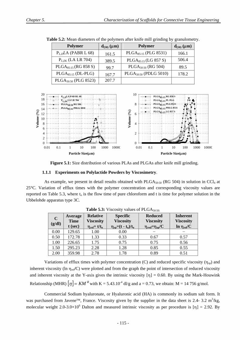
Chapter 5. Characterization of Scaffolds for Connective Tissue Engineering
- 115 -
Table 5.2: Mean diameters of the polymers after knife mill grinding by granulometry.
Polymer d(50) (m) Polymer d(50) (m)
PL,DLA (PABR L 68) 161.5 PLGA85:15 (PLG 8531) 166.1
PL,DL (LA LR 704) 389.5 PLGA85:15 (LG 857 S) 506.4
PLGA85:15 (RG 858 S) 99.7 PLGA50:50 (RG 504) 89.5
PLGA85:15 (DL-PLG) 167.7 PLGA50:50 (PDLG 5010) 178.2
PLGA50:50 (PLG 8523) 207.7
Poly (Lactide-co-glycolide) : Granulometry
Particle Size(m)
0.01 0.1 1 10 100 1000 10000
Vol
um
e (%
)
0
2
4
6
8
10
12
14
16
18
20PL,DLA PAB RL 68
PL,DLLA LR 704
PLGA50:50 RG 504
PLGA85:15 PDLG 5010
Poly (Lactide-co-glycolide) : Granulometry
Particle Size(m)
0.01 0.1 1 10 100 1000 10000
Vol
um
e (%
)
0
2
4
6
8
10PLGA85:15 RG 858 S
PLGA85:15 PL PLG
PLGA85:15 PLG 8523
PLGA85:15 PDLG 8531
PLGA85:15 LG 857 S
Figure 5.1: Size distribution of various PLAs and PLGAs after knife mill grinding.
1.1.1 Experiments on Polylactide Powders by Viscosimetry.
As example, we present in detail results obtained with PLGA50:50 (RG 504) in solution in CCl4 at 25°C. Variation of efflux times with the polymer concentration and corresponding viscosity values are reported on Table 5.3, where to is the flow time of pure chloroform and t is time for polymer solution in the
Ubbelohde apparatus type 3C.
Table 5.3: Viscosity values of PLGA50:50.
C (g/dl)
Average Time t (sec)
Relative Viscosity rel= t/to
Specific Viscosity
sp=(t - to)/to
Reduced Viscosity red=sp/C
Inherent Viscosity ln rel/C
0.00 129.65 1.00 0.00 − − 0.50 172.78 1.33 0.33 0.67 0.57 1.00 226.65 1.75 0.75 0.75 0.56 1.50 295.23 2.28 1.28 0.85 0.55 2.00 359.98 2.78 1.78 0.89 0.51
Variations of efflux times with polymer concentration (C) and reduced specific viscosity (sp) and
inherent viscosity (ln rel/C) were plotted and from the graph the point of intersection of reduced viscosity
and inherent viscosity at the Y-axis gives the intrinsic viscosity [] = 0.60. By using the Mark-Houwink
Relationship (MHR) aKM with K = 5.43.10-4 dl/g and a = 0.73, we obtain: M = 14 756 g/mol.
Commercial Sodium hyaluronate, or Hyaluronic acid (HA) is commonly its sodium salt form. It
was purchased from Javene, France. Viscosity given by the supplier in the data sheet is 2.4- 3.2 m3/kg,
molecular weight 2.0-3.0×10⁶ Dalton and measured intrinsic viscosity as per procedure is [] = 2.92. By
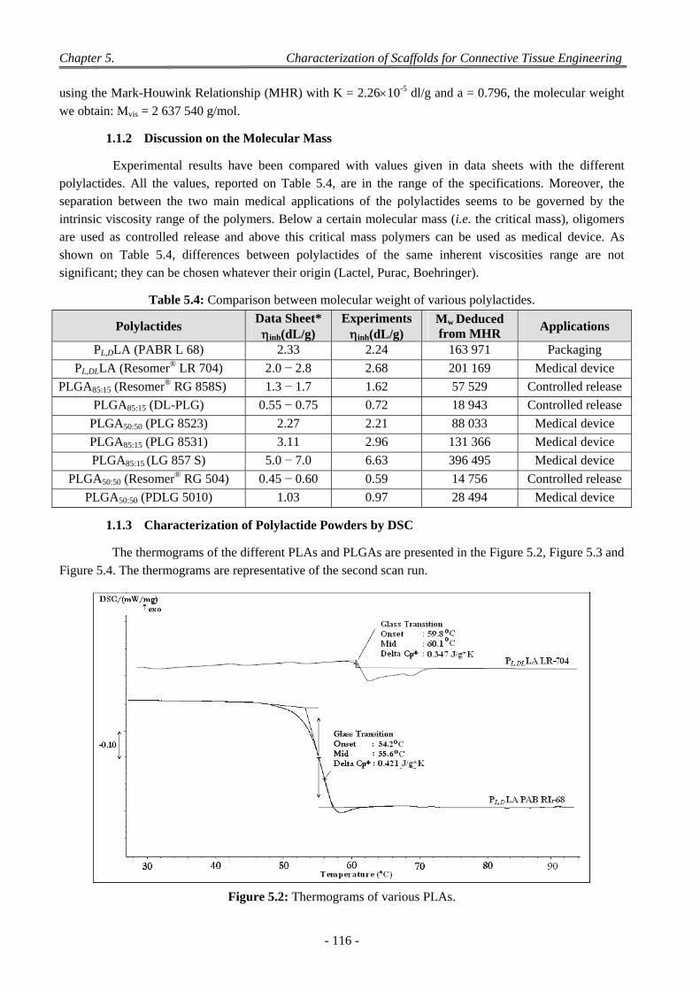
Chapter 5. Characterization of Scaffolds for Connective Tissue Engineering
- 116 -
using the Mark-Houwink Relationship (MHR) with K = 2.2610-5 dl/g and a = 0.796, the molecular weight
we obtain: Mvis = 2 637 540 g/mol.
1.1.2 Discussion on the Molecular Mass
Experimental results have been compared with values given in data sheets with the different polylactides. All the values, reported on Table 5.4, are in the range of the specifications. Moreover, the separation between the two main medical applications of the polylactides seems to be governed by the intrinsic viscosity range of the polymers. Below a certain molecular mass (i.e. the critical mass), oligomers are used as controlled release and above this critical mass polymers can be used as medical device. As shown on Table 5.4, differences between polylactides of the same inherent viscosities range are not
significant; they can be chosen whatever their origin (Lactel, Purac, Boehringer).
Table 5.4: Comparison between molecular weight of various polylactides.
Polylactides Data Sheet* inh(dL/g)
Experiments inh(dL/g)
Mw Deduced from MHR
Applications
PL,DLA (PABR L 68) 2.33 2.24 163 971 Packaging
PL,DLLA (Resomer® LR 704) 2.0 − 2.8 2.68 201 169 Medical device
PLGA85:15 (Resomer® RG 858S) 1.3 − 1.7 1.62 57 529 Controlled release
PLGA85:15 (DL-PLG) 0.55 − 0.75 0.72 18 943 Controlled release
PLGA50:50 (PLG 8523) 2.27 2.21 88 033 Medical device
PLGA85:15 (PLG 8531) 3.11 2.96 131 366 Medical device
PLGA85:15 (LG 857 S) 5.0 − 7.0 6.63 396 495 Medical device
PLGA50:50 (Resomer® RG 504) 0.45 − 0.60 0.59 14 756 Controlled release
PLGA50:50 (PDLG 5010) 1.03 0.97 28 494 Medical device
1.1.3 Characterization of Polylactide Powders by DSC
The thermograms of the different PLAs and PLGAs are presented in the Figure 5.2, Figure 5.3 and
Figure 5.4. The thermograms are representative of the second scan run.
Figure 5.2: Thermograms of various PLAs.
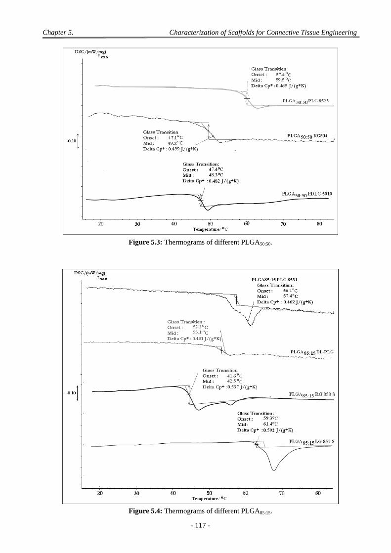
Chapter 5. Characterization of Scaffolds for Connective Tissue Engineering
- 117 -
Figure 5.3: Thermograms of different PLGA50:50.
Figure 5.4: Thermograms of different PLGA85:15.
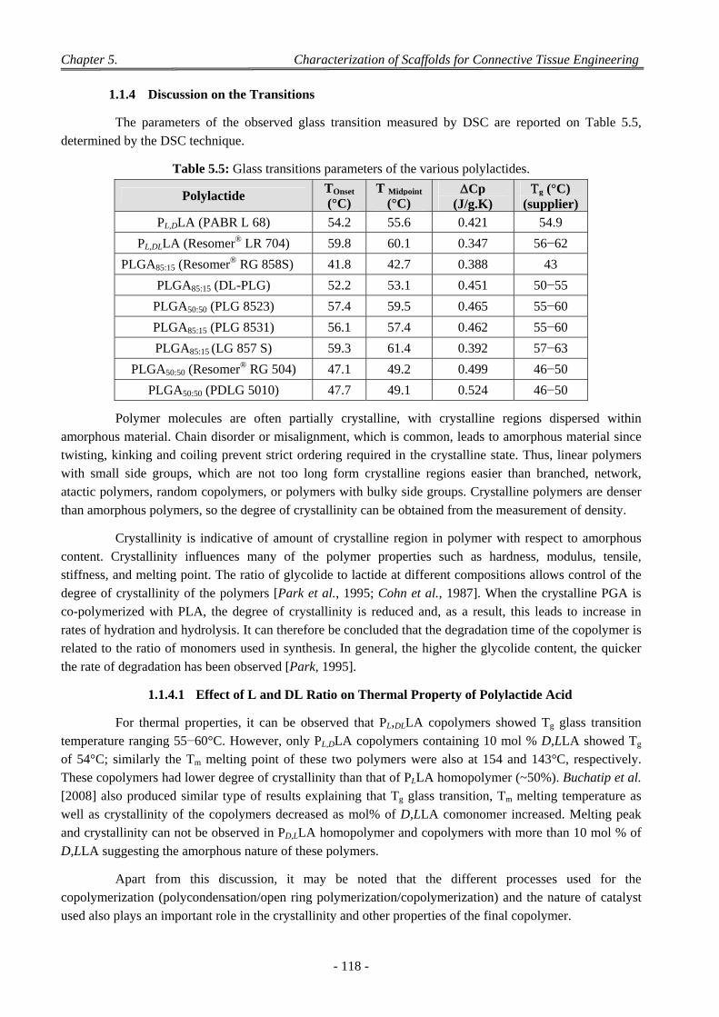
Chapter 5. Characterization of Scaffolds for Connective Tissue Engineering
- 118 -
1.1.4 Discussion on the Transitions
The parameters of the observed glass transition measured by DSC are reported on Table 5.5,
determined by the DSC technique.
Table 5.5: Glass transitions parameters of the various polylactides.
Polylactide TOnset (°C)
T Midpoint
(°C) Cp
(J/g.K) g (°C)
(supplier) PL,DLA (PABR L 68) 54.2 55.6 0.421 54.9
PL,DLLA (Resomer® LR 704) 59.8 60.1 0.347 56−62
PLGA85:15 (Resomer® RG 858S) 41.8 42.7 0.388 43
PLGA85:15 (DL-PLG) 52.2 53.1 0.451 50−55
PLGA50:50 (PLG 8523) 57.4 59.5 0.465 55−60
PLGA85:15 (PLG 8531) 56.1 57.4 0.462 55−60
PLGA85:15 (LG 857 S) 59.3 61.4 0.392 57−63
PLGA50:50 (Resomer® RG 504) 47.1 49.2 0.499 46−50
PLGA50:50 (PDLG 5010) 47.7 49.1 0.524 46−50
Polymer molecules are often partially crystalline, with crystalline regions dispersed within amorphous material. Chain disorder or misalignment, which is common, leads to amorphous material since twisting, kinking and coiling prevent strict ordering required in the crystalline state. Thus, linear polymers with small side groups, which are not too long form crystalline regions easier than branched, network, atactic polymers, random copolymers, or polymers with bulky side groups. Crystalline polymers are denser
than amorphous polymers, so the degree of crystallinity can be obtained from the measurement of density.
Crystallinity is indicative of amount of crystalline region in polymer with respect to amorphous content. Crystallinity influences many of the polymer properties such as hardness, modulus, tensile, stiffness, and melting point. The ratio of glycolide to lactide at different compositions allows control of the degree of crystallinity of the polymers [Park et al., 1995; Cohn et al., 1987]. When the crystalline PGA is co-polymerized with PLA, the degree of crystallinity is reduced and, as a result, this leads to increase in rates of hydration and hydrolysis. It can therefore be concluded that the degradation time of the copolymer is related to the ratio of monomers used in synthesis. In general, the higher the glycolide content, the quicker
the rate of degradation has been observed [Park, 1995].
1.1.4.1 Effect of L and DL Ratio on Thermal Property of Polylactide Acid
For thermal properties, it can be observed that PL,DLLA copolymers showed Tg glass transition temperature ranging 55−60°C. However, only PL,DLA copolymers containing 10 mol % D,LLA showed Tg of 54°C; similarly the Tm melting point of these two polymers were also at 154 and 143°C, respectively. These copolymers had lower degree of crystallinity than that of PLLA homopolymer (~50%). Buchatip et al. [2008] also produced similar type of results explaining that Tg glass transition, Tm melting temperature as well as crystallinity of the copolymers decreased as mol% of D,LLA comonomer increased. Melting peak and crystallinity can not be observed in PD,LLA homopolymer and copolymers with more than 10 mol % of
D,LLA suggesting the amorphous nature of these polymers.
Apart from this discussion, it may be noted that the different processes used for the copolymerization (polycondensation/open ring polymerization/copolymerization) and the nature of catalyst
used also plays an important role in the crystallinity and other properties of the final copolymer.
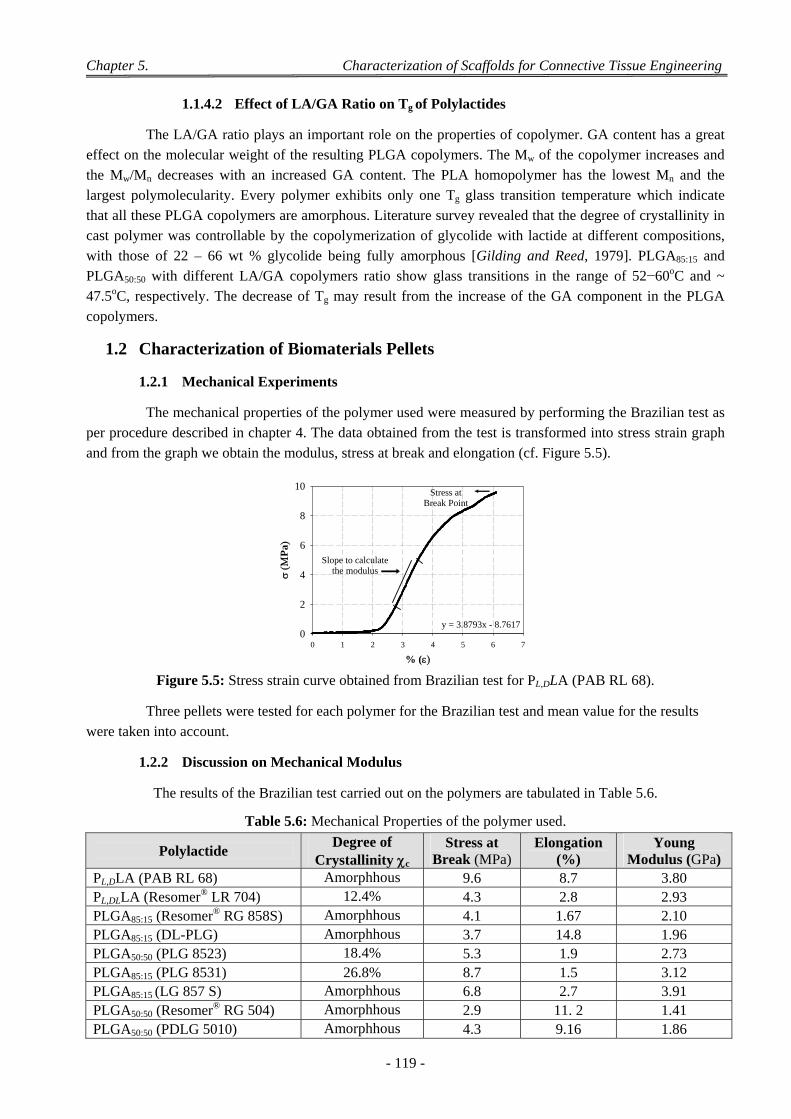
Chapter 5. Characterization of Scaffolds for Connective Tissue Engineering
- 119 -
1.1.4.2 Effect of LA/GA Ratio on Tg of Polylactides
The LA/GA ratio plays an important role on the properties of copolymer. GA content has a great effect on the molecular weight of the resulting PLGA copolymers. The Mw of the copolymer increases and the Mw/Mn decreases with an increased GA content. The PLA homopolymer has the lowest Mn and the largest polymolecularity. Every polymer exhibits only one Tg glass transition temperature which indicate that all these PLGA copolymers are amorphous. Literature survey revealed that the degree of crystallinity in cast polymer was controllable by the copolymerization of glycolide with lactide at different compositions, with those of 22 – 66 wt % glycolide being fully amorphous [Gilding and Reed, 1979]. PLGA85:15 and PLGA50:50 with different LA/GA copolymers ratio show glass transitions in the range of 52−60oC and ~ 47.5oC, respectively. The decrease of Tg may result from the increase of the GA component in the PLGA
copolymers.
1.2 Characterization of Biomaterials Pellets
1.2.1 Mechanical Experiments
The mechanical properties of the polymer used were measured by performing the Brazilian test as per procedure described in chapter 4. The data obtained from the test is transformed into stress strain graph
and from the graph we obtain the modulus, stress at break and elongation (cf. Figure 5.5).
Tg Experimental and Source values
% (0 1 2 3 4 5 6 7
Pa
0
2
4
6
8
10Stress at
Break Point
y = 3.8793x - 8.7617
Slope to calculate the modulus
Figure 5.5: Stress strain curve obtained from Brazilian test for PL,DLA (PAB RL 68).
Three pellets were tested for each polymer for the Brazilian test and mean value for the results
were taken into account.
1.2.2 Discussion on Mechanical Modulus
The results of the Brazilian test carried out on the polymers are tabulated in Table 5.6.
Table 5.6: Mechanical Properties of the polymer used.
Polylactide Degree of
Crystallinity c Stress at
Break (MPa) Elongation
(%) Young
Modulus (GPa) PL,DLA (PAB RL 68) Amorphhous 9.6 8.7 3.80 PL,DLLA (Resomer® LR 704) 12.4% 4.3 2.8 2.93 PLGA85:15 (Resomer® RG 858S) Amorphhous 4.1 1.67 2.10 PLGA85:15 (DL-PLG) Amorphhous 3.7 14.8 1.96 PLGA50:50 (PLG 8523) 18.4% 5.3 1.9 2.73 PLGA85:15 (PLG 8531) 26.8% 8.7 1.5 3.12 PLGA85:15 (LG 857 S) Amorphhous 6.8 2.7 3.91 PLGA50:50 (Resomer® RG 504) Amorphhous 2.9 11. 2 1.41 PLGA50:50 (PDLG 5010) Amorphhous 4.3 9.16 1.86
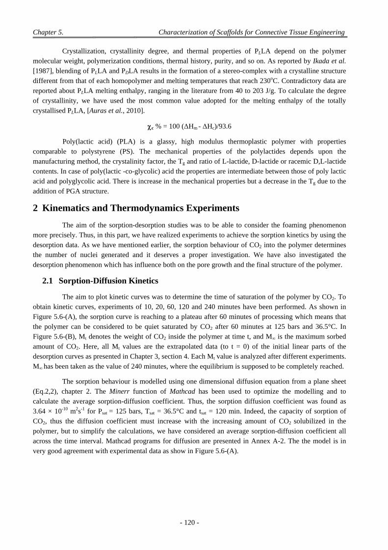
Chapter 5. Characterization of Scaffolds for Connective Tissue Engineering
- 120 -
Crystallization, crystallinity degree, and thermal properties of PLLA depend on the polymer molecular weight, polymerization conditions, thermal history, purity, and so on. As reported by Ikada et al. [1987], blending of PLLA and PDLA results in the formation of a stereo-complex with a crystalline structure different from that of each homopolymer and melting temperatures that reach 230oC. Contradictory data are reported about PLLA melting enthalpy, ranging in the literature from 40 to 203 J/g. To calculate the degree of crystallinity, we have used the most common value adopted for the melting enthalpy of the totally
crystallised PLLA, [Auras et al., 2010].
c % = 100 (ΔHm - ΔHc)/93.6
Poly(lactic acid) (PLA) is a glassy, high modulus thermoplastic polymer with properties comparable to polystyrene (PS). The mechanical properties of the polylactides depends upon the manufacturing method, the crystalinity factor, the Tg and ratio of L-lactide, D-lactide or racemic D,L-lactide contents. In case of poly(lactic -co-glycolic) acid the properties are intermediate between those of poly lactic acid and polyglycolic acid. There is increase in the mechanical properties but a decrease in the Tg due to the
addition of PGA structure.
2 Kinematics and Thermodynamics Experiments
The aim of the sorption-desorption studies was to be able to consider the foaming phenomenon more precisely. Thus, in this part, we have realized experiments to achieve the sorption kinetics by using the desorption data. As we have mentioned earlier, the sorption behaviour of CO2 into the polymer determines the number of nuclei generated and it deserves a proper investigation. We have also investigated the
desorption phenomenon which has influence both on the pore growth and the final structure of the polymer.
2.1 Sorption-Diffusion Kinetics
The aim to plot kinetic curves was to determine the time of saturation of the polymer by CO2. To obtain kinetic curves, experiments of 10, 20, 60, 120 and 240 minutes have been performed. As shown in Figure 5.6-(A), the sorption curve is reaching to a plateau after 60 minutes of processing which means that the polymer can be considered to be quiet saturated by CO2 after 60 minutes at 125 bars and 36.5°C. In Figure 5.6-(B), Mt denotes the weight of CO2 inside the polymer at time t, and M∞ is the maximum sorbed amount of CO2. Here, all Mt values are the extrapolated data (to t = 0) of the initial linear parts of the desorption curves as presented in Chapter 3, section 4. Each Mt value is analyzed after different experiments.
M∞ has been taken as the value of 240 minutes, where the equilibrium is supposed to be completely reached.
The sorption behaviour is modelled using one dimensional diffusion equation from a plane sheet (Eq.2,2), chapter 2. The Minerr function of Mathcad has been used to optimize the modelling and to calculate the average sorption-diffusion coefficient. Thus, the sorption diffusion coefficient was found as 3.64 × 10⁻¹⁰ m2s-1 for Psat = 125 bars, Tsat = 36.5°C and tsat = 120 min. Indeed, the capacity of sorption of CO2, thus the diffusion coefficient must increase with the increasing amount of CO2 solubilized in the polymer, but to simplify the calculations, we have considered an average sorption-diffusion coefficient all across the time interval. Mathcad programs for diffusion are presented in Annex A-2. The the model is in
very good agreement with experimental data as show in Figure 5.6-(A).
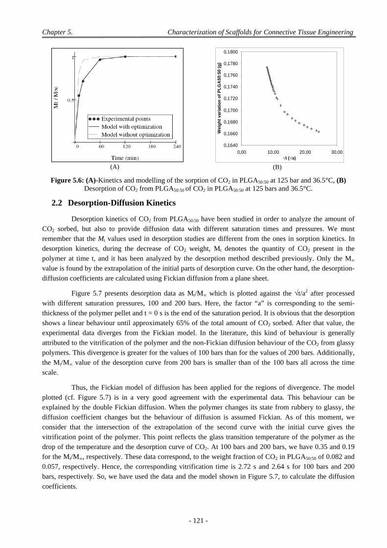
Chapter 5. Characterization of Scaffolds for Connective Tissue Engineering
- 121 -
Figure 5.6: (A)-Kinetics and modelling of the sorption of CO2 in PLGA50:50 at 125 bar and 36.5°C, (B)
Desorption of CO2 from PLGA50:50 of CO2 in PLGA50:50 at 125 bars and 36.5°C.
2.2 Desorption-Diffusion Kinetics
Desorption kinetics of CO2 from PLGA50:50 have been studied in order to analyze the amount of CO2 sorbed, but also to provide diffusion data with different saturation times and pressures. We must remember that the Mt values used in desorption studies are different from the ones in sorption kinetics. In desorption kinetics, during the decrease of CO2 weight, Mt denotes the quantity of CO2 present in the polymer at time t, and it has been analyzed by the desorption method described previously. Only the M∞ value is found by the extrapolation of the initial parts of desorption curve. On the other hand, the desorption-
diffusion coefficients are calculated using Fickian diffusion from a plane sheet.
Figure 5.7 presents desorption data as Mt/M∞ which is plotted against the √t/a2 after processed with different saturation pressures, 100 and 200 bars. Here, the factor “a” is corresponding to the semi-thickness of the polymer pellet and t = 0 s is the end of the saturation period. It is obvious that the desorption shows a linear behaviour until approximately 65% of the total amount of CO2 sorbed. After that value, the experimental data diverges from the Fickian model. In the literature, this kind of behaviour is generally attributed to the vitrification of the polymer and the non-Fickian diffusion behaviour of the CO2 from glassy polymers. This divergence is greater for the values of 100 bars than for the values of 200 bars. Additionally, the Mt/M∞ value of the desorption curve from 200 bars is smaller than of the 100 bars all across the time
scale.
Thus, the Fickian model of diffusion has been applied for the regions of divergence. The model plotted (cf. Figure 5.7) is in a very good agreement with the experimental data. This behaviour can be explained by the double Fickian diffusion. When the polymer changes its state from rubbery to glassy, the diffusion coefficient changes but the behaviour of diffusion is assumed Fickian. As of this moment, we consider that the intersection of the extrapolation of the second curve with the initial curve gives the vitrification point of the polymer. This point reflects the glass transition temperature of the polymer as the drop of the temperature and the desorption curve of CO2. At 100 bars and 200 bars, we have 0.35 and 0.19 for the Mt/M∞, respectively. These data correspond, to the weight fraction of CO2 in PLGA50:50 of 0.082 and 0.057, respectively. Hence, the corresponding vitrification time is 2.72 s and 2.64 s for 100 bars and 200 bars, respectively. So, we have used the data and the model shown in Figure 5.7, to calculate the diffusion
coefficients.
(A)
0,1640
0,1660
0,1680
0,1700
0,1720
0,1740
0,1760
0,1780
0,1800
0,00 10,00 20,00 30,00√t (√s)
Wei
gh
t va
riat
ion
of
PL
GA
50:5
0 (g
)
(B)
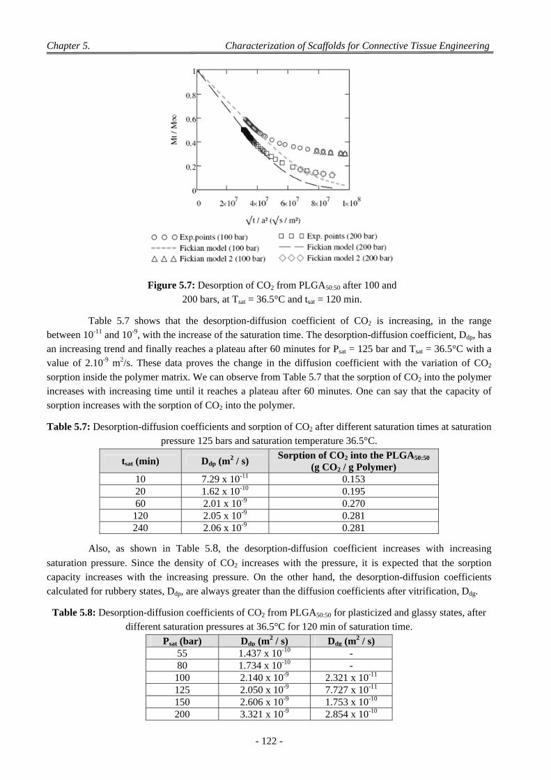
Chapter 5. Characterization of Scaffolds for Connective Tissue Engineering
- 122 -
Figure 5.7: Desorption of CO2 from PLGA50:50 after 100 and 200 bars, at Tsat = 36.5°C and tsat = 120 min.
Table 5.7 shows that the desorption-diffusion coefficient of CO2 is increasing, in the range between 10-11 and 10-9, with the increase of the saturation time. The desorption-diffusion coefficient, Ddp, has an increasing trend and finally reaches a plateau after 60 minutes for Psat = 125 bar and Tsat = 36.5°C with a value of 2.10-9 m2/s. These data proves the change in the diffusion coefficient with the variation of CO2 sorption inside the polymer matrix. We can observe from Table 5.7 that the sorption of CO2 into the polymer increases with increasing time until it reaches a plateau after 60 minutes. One can say that the capacity of
sorption increases with the sorption of CO2 into the polymer.
Table 5.7: Desorption-diffusion coefficients and sorption of CO2 after different saturation times at saturation pressure 125 bars and saturation temperature 36.5°C.
tsat (min) Ddp (m2 / s) Sorption of CO2 into the PLGA50:50
(g CO2 / g Polymer) 10 7.29 x 10⁻¹¹ 0.153 20 1.62 x 10⁻¹⁰ 0.195 60 2.01 x 10⁻⁹ 0.270
120 2.05 x 10⁻⁹ 0.281 240 2.06 x 10⁻⁹ 0.281
Also, as shown in Table 5.8, the desorption-diffusion coefficient increases with increasing
saturation pressure. Since the density of CO2 increases with the pressure, it is expected that the sorption capacity increases with the increasing pressure. On the other hand, the desorption-diffusion coefficients
calculated for rubbery states, Ddp, are always greater than the diffusion coefficients after vitrification, Ddg.
Table 5.8: Desorption-diffusion coefficients of CO2 from PLGA50:50 for plasticized and glassy states, after different saturation pressures at 36.5°C for 120 min of saturation time.
Psat (bar) Ddp (m2 / s) Ddg (m2 / s)
55 1.437 x 10⁻¹⁰ - 80 1.734 x 10⁻¹⁰ -
100 2.140 x 10⁻⁹ 2.321 x 10⁻¹¹ 125 2.050 x 10⁻⁹ 7.727 x 10⁻¹¹ 150 2.606 x 10⁻⁹ 1.753 x 10⁻¹⁰ 200 3.321 x 10⁻⁹ 2.854 x 10⁻¹⁰
Chapter 5. Characterization of Scaffolds for Connective Tissue Engineering
- 123 -
2.3 The Sorption Isotherm
By using desorption kinetics, the initial points of desorption have been extrapolated to t = 0 s and the amount of CO2 sorbed by the polymer is analyzed. We underline that here, t = 0 s is the end of the saturation period. One can remember that the nucleation rate is related to the CO2 at the end of the saturation period. Thus, we must know how much CO2 is sorbed by the polymer to calculate the nucleation rate. All experiments have been carried out at 36.5°C during 120 minutes with different pressure conditions. The pressure conditions and the corresponding sorption data is presented in Table 5.9. It has been observed that
the sorption increases monotonically with the pressure.
Table 5.9: Sorption data for PLGA50:50 at 36.5°C.
P (bar) Average Sorption Data
(gCO2 /g Polymer) 55 0.112 80 0.207
100 0.258 125 0.281 150 0.296 200 0.333
Experimental results and model predictions are presented with the literature data in Figure 5.8. A significant change in slope is appeared within the interval of 70-80 bars. The change in the slope can be
explained by the transition of the CO2 rich phase from gas to the much denser supercritical state.
Figure 5.8: Sorption isotherm of CO2 into PLGA50:50. [Pini et al., 2008]
Our sorption isotherm and modelling with SL-EOS, is in agreement with those reported by Pini et al. [2008]. Our experimental points were always approximately 5% lower than the literature data which can be attributed to the small temperature difference. Indeed, the density of CO2, so the sorption decreases with the temperature. Additionally, under the critical point of CO2, SL-EOS diverges from the experimental data.
But, it has good estimations above critical point for the sorption.
Furthermore, since we have investigated the sorption kinetics earlier, we have also a sorption
kinetic data. This evaluation was presented in Table 5.8 and found to increase with time until it reaches a
plateau after 60 minutes. If we interpolate the isothermal sorption data for 120 minutes (Figure 5.8 and Table 5.9) between 55 and 80 bars, a sorption value of 0.195 can be found for 76.2 bars. This value is equal to the
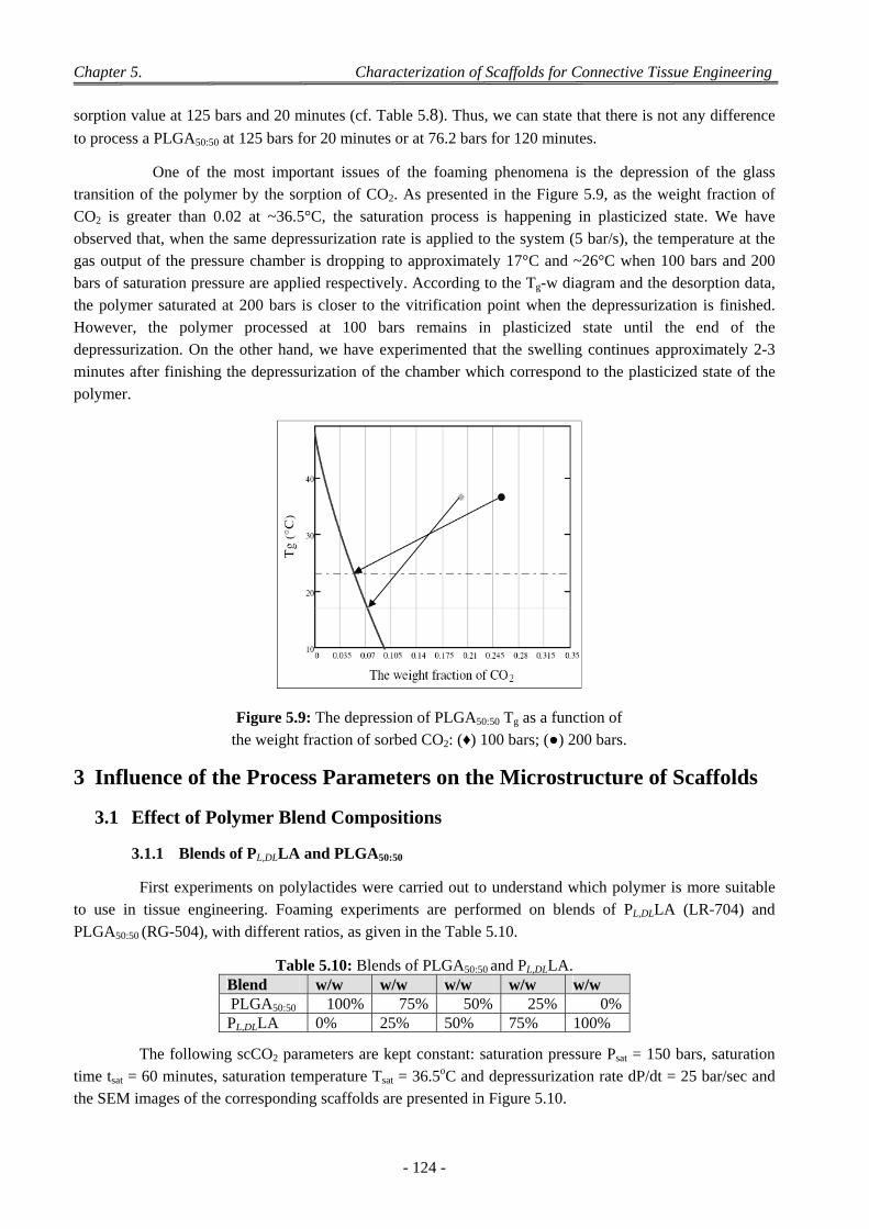
Chapter 5. Characterization of Scaffolds for Connective Tissue Engineering
- 124 -
sorption value at 125 bars and 20 minutes (cf. Table 5.8). Thus, we can state that there is not any difference
to process a PLGA50:50 at 125 bars for 20 minutes or at 76.2 bars for 120 minutes.
One of the most important issues of the foaming phenomena is the depression of the glass transition of the polymer by the sorption of CO2. As presented in the Figure 5.9, as the weight fraction of CO2 is greater than 0.02 at ~36.5°C, the saturation process is happening in plasticized state. We have observed that, when the same depressurization rate is applied to the system (5 bar/s), the temperature at the gas output of the pressure chamber is dropping to approximately 17°C and ~26°C when 100 bars and 200 bars of saturation pressure are applied respectively. According to the Tg-w diagram and the desorption data, the polymer saturated at 200 bars is closer to the vitrification point when the depressurization is finished. However, the polymer processed at 100 bars remains in plasticized state until the end of the depressurization. On the other hand, we have experimented that the swelling continues approximately 2-3 minutes after finishing the depressurization of the chamber which correspond to the plasticized state of the
polymer.
Figure 5.9: The depression of PLGA50:50 Tg as a function of the weight fraction of sorbed CO2: (♦) 100 bars; (●) 200 bars.
3 Influence of the Process Parameters on the Microstructure of Scaffolds
3.1 Effect of Polymer Blend Compositions
3.1.1 Blends of PL,DLLA and PLGA50:50
First experiments on polylactides were carried out to understand which polymer is more suitable to use in tissue engineering. Foaming experiments are performed on blends of PL,DLLA (LR-704) and
PLGA50:50 (RG-504), with different ratios, as given in the Table 5.10.
Table 5.10: Blends of PLGA50:50 and PL,DLLA. Blend w/w w/w w/w w/w w/w PLGA50:50 100% 75% 50% 25% 0% PL,DLLA 0% 25% 50% 75% 100%
The following scCO2 parameters are kept constant: saturation pressure Psat = 150 bars, saturation time tsat = 60 minutes, saturation temperature Tsat = 36.5oC and depressurization rate dP/dt = 25 bar/sec and the SEM images of the corresponding scaffolds are presented in Figure 5.10.
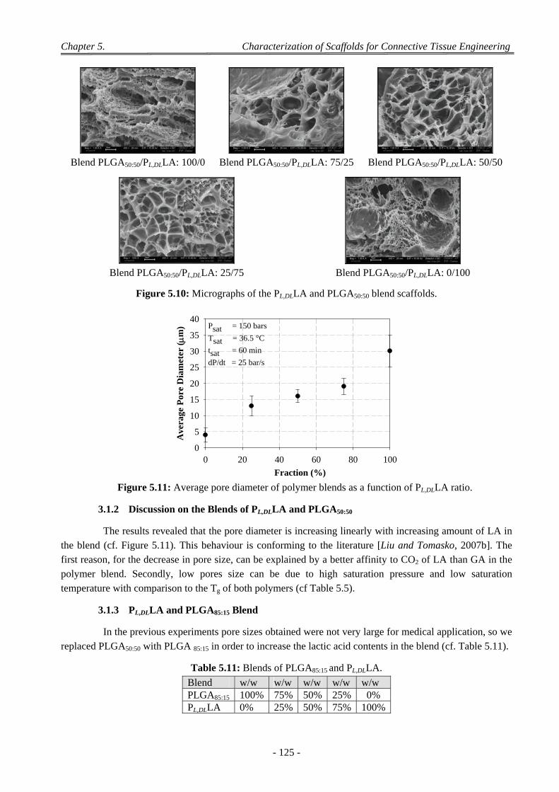
Chapter 5. Characterization of Scaffolds for Connective Tissue Engineering
- 125 -
Blend PLGA50:50/PL,DLLA: 100/0 Blend PLGA50:50/PL,DLLA: 75/25 Blend PLGA50:50/PL,DLLA: 50/50
Blend PLGA50:50/PL,DLLA: 25/75 Blend PLGA50:50/PL,DLLA: 0/100
Figure 5.10: Micrographs of the PL,DLLA and PLGA50:50 blend scaffolds.
PL,DLLA and PLGA50:50 Blend
Fraction (%)
0 20 40 60 80 100
Ave
rage
Por
e D
iam
eter
(m
)
0
5
10
15
20
25
30
35
40Psat = 150 bars
Tsat = 36.5 °C
tsat = 60 min
dP/dt = 25 bar/s
Figure 5.11: Average pore diameter of polymer blends as a function of PL,DLLA ratio.
3.1.2 Discussion on the Blends of PL,DLLA and PLGA50:50
The results revealed that the pore diameter is increasing linearly with increasing amount of LA in the blend (cf. Figure 5.11). This behaviour is conforming to the literature [Liu and Tomasko, 2007b]. The first reason, for the decrease in pore size, can be explained by a better affinity to CO2 of LA than GA in the polymer blend. Secondly, low pores size can be due to high saturation pressure and low saturation
temperature with comparison to the Tg of both polymers (cf Table 5.5).
3.1.3 PL,DLLA and PLGA85:15 Blend
In the previous experiments pore sizes obtained were not very large for medical application, so we
replaced PLGA50:50 with PLGA 85:15 in order to increase the lactic acid contents in the blend (cf. Table 5.11).
Table 5.11: Blends of PLGA85:15 and PL,DLLA.
Blend w/w w/w w/w w/w w/w PLGA85:15 100% 75% 50% 25% 0% PL,DLLA 0% 25% 50% 75% 100%
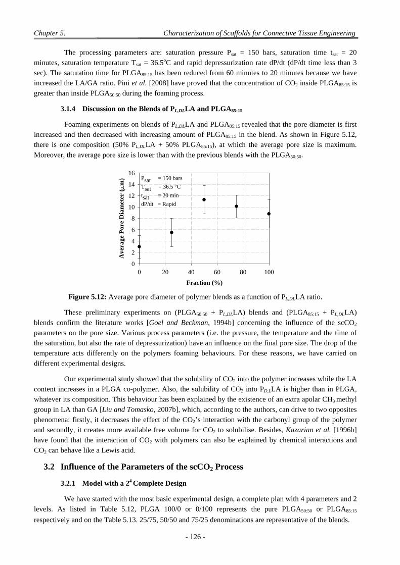
Chapter 5. Characterization of Scaffolds for Connective Tissue Engineering
- 126 -
The processing parameters are: saturation pressure Psat = 150 bars, saturation time tsat = 20 minutes, saturation temperature Tsat = 36.5oC and rapid depressurization rate dP/dt (dP/dt time less than 3 sec). The saturation time for PLGA85:15 has been reduced from 60 minutes to 20 minutes because we have increased the LA/GA ratio. Pini et al. [2008] have proved that the concentration of CO2 inside PLGA85:15 is
greater than inside PLGA50:50 during the foaming process.
3.1.4 Discussion on the Blends of PL,DLLA and PLGA85:15
Foaming experiments on blends of PL,DLLA and PLGA85:15 revealed that the pore diameter is first increased and then decreased with increasing amount of PLGA85:15 in the blend. As shown in Figure 5.12, there is one composition (50% PL,DLLA + 50% PLGA85:15), at which the average pore size is maximum.
Moreover, the average pore size is lower than with the previous blends with the PLGA50:50.
PL,DLLA and PLGA85:15 Blend
Fraction (%)
0 20 40 60 80 100
Ave
rage
Por
e D
iam
eter
(m
)
0
2
4
6
8
10
12
14
16Psat = 150 bars
Tsat = 36.5 °C
tsat = 20 min
dP/dt = Rapid
Figure 5.12: Average pore diameter of polymer blends as a function of PL,DLLA ratio.
These preliminary experiments on (PLGA50:50 + PL,DLLA) blends and (PLGA85:15 + PL,DLLA) blends confirm the literature works [Goel and Beckman, 1994b] concerning the influence of the scCO2 parameters on the pore size. Various process parameters (i.e. the pressure, the temperature and the time of the saturation, but also the rate of depressurization) have an influence on the final pore size. The drop of the temperature acts differently on the polymers foaming behaviours. For these reasons, we have carried on
different experimental designs.
Our experimental study showed that the solubility of CO2 into the polymer increases while the LA content increases in a PLGA co-polymer. Also, the solubility of CO2 into PD,LLA is higher than in PLGA, whatever its composition. This behaviour has been explained by the existence of an extra apolar CH3 methyl group in LA than GA [Liu and Tomasko, 2007b], which, according to the authors, can drive to two opposites phenomena: firstly, it decreases the effect of the CO2’s interaction with the carbonyl group of the polymer and secondly, it creates more available free volume for CO2 to solubilise. Besides, Kazarian et al. [1996b] have found that the interaction of CO2 with polymers can also be explained by chemical interactions and
CO2 can behave like a Lewis acid.
3.2 Influence of the Parameters of the scCO2 Process
3.2.1 Model with a 24 Complete Design
We have started with the most basic experimental design, a complete plan with 4 parameters and 2 levels. As listed in Table 5.12, PLGA 100/0 or 0/100 represents the pure PLGA50:50 or PLGA85:15
respectively and on the Table 5.13. 25/75, 50/50 and 75/25 denominations are representative of the blends.
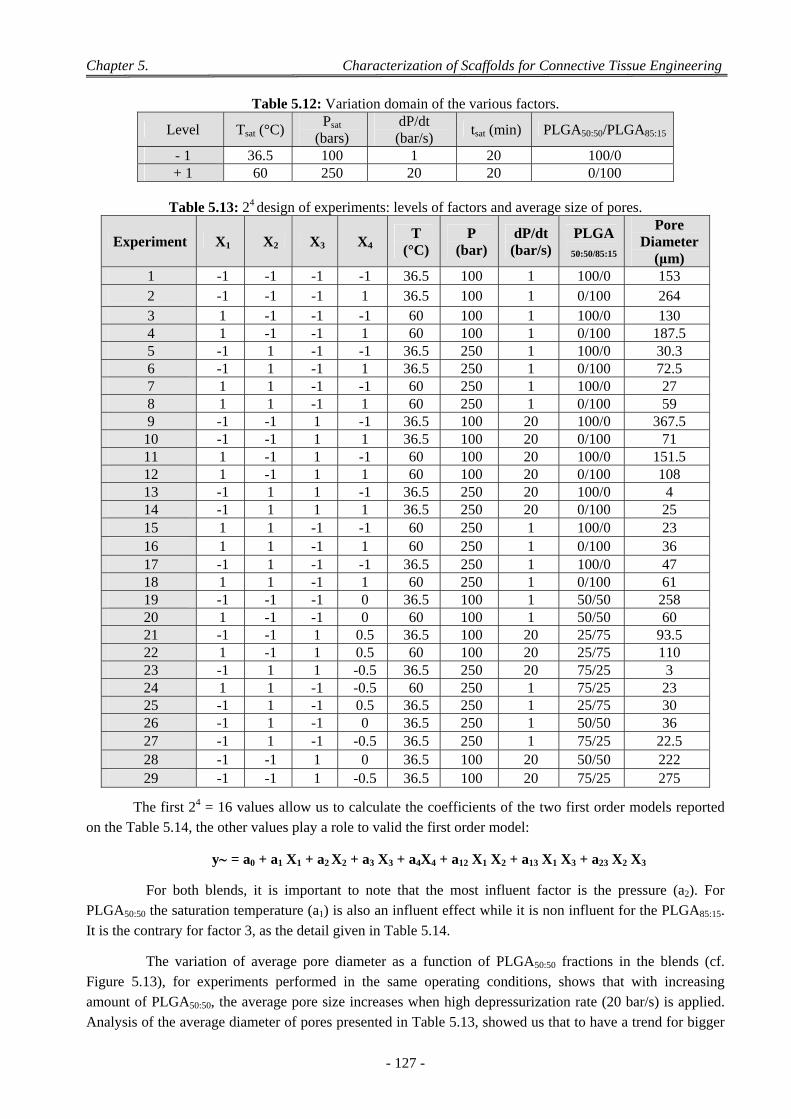
Chapter 5. Characterization of Scaffolds for Connective Tissue Engineering
- 127 -
Table 5.12: Variation domain of the various factors.
Level Tsat (°C) Psat
(bars) dP/dt (bar/s)
tsat (min) PLGA50:50/PLGA85:15
- 1 36.5 100 1 20 100/0 + 1 60 250 20 20 0/100
Table 5.13: 24 design of experiments: levels of factors and average size of pores.
Experiment X1 X2 X3 X4 T
(°C) P
(bar) dP/dt
(bar/s)PLGA
50:50/85:15
Pore Diameter
(μm) 1 -1 -1 -1 -1 36.5 100 1 100/0 153 2 -1 -1 -1 1 36.5 100 1 0/100 264 3 1 -1 -1 -1 60 100 1 100/0 130 4 1 -1 -1 1 60 100 1 0/100 187.5 5 -1 1 -1 -1 36.5 250 1 100/0 30.3 6 -1 1 -1 1 36.5 250 1 0/100 72.5 7 1 1 -1 -1 60 250 1 100/0 27 8 1 1 -1 1 60 250 1 0/100 59 9 -1 -1 1 -1 36.5 100 20 100/0 367.5
10 -1 -1 1 1 36.5 100 20 0/100 71 11 1 -1 1 -1 60 100 20 100/0 151.5 12 1 -1 1 1 60 100 20 0/100 108 13 -1 1 1 -1 36.5 250 20 100/0 4 14 -1 1 1 1 36.5 250 20 0/100 25 15 1 1 -1 -1 60 250 1 100/0 23 16 1 1 -1 1 60 250 1 0/100 36 17 -1 1 -1 -1 36.5 250 1 100/0 47 18 1 1 -1 1 60 250 1 0/100 61 19 -1 -1 -1 0 36.5 100 1 50/50 258 20 1 -1 -1 0 60 100 1 50/50 60 21 -1 -1 1 0.5 36.5 100 20 25/75 93.5 22 1 -1 1 0.5 60 100 20 25/75 110 23 -1 1 1 -0.5 36.5 250 20 75/25 3 24 1 1 -1 -0.5 60 250 1 75/25 23 25 -1 1 -1 0.5 36.5 250 1 25/75 30 26 -1 1 -1 0 36.5 250 1 50/50 36 27 -1 1 -1 -0.5 36.5 250 1 75/25 22.5 28 -1 -1 1 0 36.5 100 20 50/50 222 29 -1 -1 1 -0.5 36.5 100 20 75/25 275
The first 24 = 16 values allow us to calculate the coefficients of the two first order models reported on the Table 5.14, the other values play a role to valid the first order model:
y = a0 + a1 X1 + a2 X2 + a3 X3 + a4X4 + a12 X1 X2 + a13 X1 X3 + a23 X2 X3
For both blends, it is important to note that the most influent factor is the pressure (a2). For PLGA50:50 the saturation temperature (a1) is also an influent effect while it is non influent for the PLGA85:15.
It is the contrary for factor 3, as the detail given in Table 5.14.
The variation of average pore diameter as a function of PLGA50:50 fractions in the blends (cf. Figure 5.13), for experiments performed in the same operating conditions, shows that with increasing amount of PLGA50:50, the average pore size increases when high depressurization rate (20 bar/s) is applied. Analysis of the average diameter of pores presented in Table 5.13, showed us that to have a trend for bigger
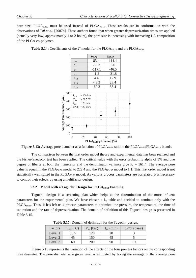
Chapter 5. Characterization of Scaffolds for Connective Tissue Engineering
- 128 -
pore size, PLGA50:50 must be used instead of PLGA85:15. These results are in conformation with the observations of Tai et al. [2007b]. These authors found that when greater depressurization times are applied (actually very low, approximately 1 to 2 hours), the pore size is increasing with increasing LA composition
of the PLGA co-polymer.
Table 5.14: Coefficients of the 24 model for the PLGA85:15 and the PLGA50:50.
â50-50 â85-15 a0 83.4 111.1 a1 -55.3 3.0 a2 -117.1 -46.5 a3 -1.2 -31.8 a12 4.4 12.9 a13 -48.3 28.4 a23 -60.2 36.4
PLGA50:50 + PLGA85:15 Blend
PLGA50:50 Fraction (%) 0 20 40 60 80 100
Ave
rage
Por
e D
iam
eter
(m
)
0
100
200
300
400
500Psat = 100 bars
Tsat = 36.5 °C
tsat = 20 min
dP/dt = 25 bar/s
Figure 5.13: Average pore diameter as a function of PLGA50:50 ratio in the PLGA50:50/PLGA85:15 blends.
The comparison between the first order model theory and experimental data has been realized and the Fisher-Snedecor test has been applied. The critical value with the error probability alpha of 5% and one degree of liberty at both the numerator and the denominator variance give Fc = 161.4. The average pore value is equal, in the PLGA50:50 model to 222.4 and the PLGA85: 15 model to 1.1. This first order model is not statistically well suited in the PLGA50:50 model. As various process parameters are correlated, it is necessary
to control their effects by using a multifactor design.
3.2.2 Model with a Taguchi’ Design for PLGA50:50 Foaming
Taguchi’ design is a screening plan which helps at the determination of the more influent parameters for the experimental plan. We have chosen a L9 table and decided to continue only with the PLGA50:50. Thus, it has left us 4 process parameters to optimize: the pressure, the temperature, the time of saturation and the rate of depressurization. The domain of definition of this Taguchi design is presented in
Table 5.15.
Table 5.15: Domain of definition for the Taguchi’ design.
Factors Tsat (°C) Psat (bar) tsat (min) dP/dt (bar/s) Level 1 36.5 120 20 3 Level 2 45 150 45 5 Level 3 60 200 90 10
Figure 5.15 represents the variation of the effects of the four process factors on the corresponding pore diameter. The pore diameter at a given level is estimated by taking the average of the average pore
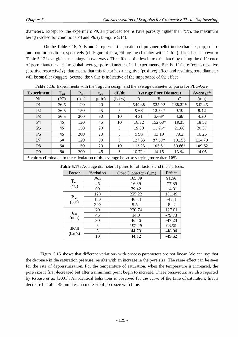
Chapter 5. Characterization of Scaffolds for Connective Tissue Engineering
- 129 -
diameters. Except for the experiment P9, all produced foams have porosity higher than 75%, the maximum
being reached for conditions P4 and P6. (cf. Figure 5.14).
On the Table 5.16, A, B and C represent the position of polymer pellet in the chamber, top, centre and bottom position respectively (cf. Figure 4.12-a, Filling the chamber with Teflon). The effects shown in Table 5.17 have global meanings in two ways. The effects of a level are calculated by taking the difference of pore diameter and the global average pore diameter of all experiments. Firstly, if the effect is negative (positive respectively), that means that this factor has a negative (positive) effect and resulting pore diameter
will be smaller (bigger). Second, the value is indicative of the importance of the effect.
Table 5.16: Experiments with the Taguchi design and the average diameter of pores for PLGA50:50.
Experiment Tsat Psat tsat dP/dt Average Pore Diameter Average*Nr. (°C) (bar) (min) (bar/s) A B C (μm) P1 36.5 120 20 3 549.88 535.02 268.32* 542.45 P2 36.5 150 45 5 9.66 12.54* 9.19 9.42 P3 36.5 200 90 10 4.31 3.66* 4.29 4.30 P4 45 120 45 10 18.82 152.68* 18.25 18.53 P5 45 150 90 3 19.08 11.96* 21.66 20.37 P6 45 200 20 5 9.98 13.19 7.62 10.26 P7 60 120 90 5 127.83 87.50* 101.56 114.70 P8 60 150 20 10 113.23 105.81 80.66* 109.52 P9 60 200 45 3 10.72* 14.15 13.94 14.05
* values eliminated in the calculation of the average because varying more than 10%
Table 5.17: Average diameter of pores for all factors and their effects.
Factor Variation <Pore Diameter (m) Effect
Tsat (°C)
36.5 185.39 91.66 45 16.39 -77.35 60 79.42 -14.31
Psat (bar)
120 225.22 131.49 150 46.84 -47.3 200 9.54 -84.2
tsat (min)
20 220.74 127.01 45 14.0 -79.73 90 46.46 -47.28
dP/dt (bar/s)
3 192.29 98.55 5 44.79 -48.94
10 44.12 -49.62
Figure 5.15 shows that different variations with process parameters are not linear. We can say that the decrease in the saturation pressure, results with an increase in the pore size. The same effect can be seen for the rate of depressurization. For the temperature of saturation, when the temperature is increased, the pore size is first decreased but after a minimum point begin to increase. These behaviours are also reported by Krause et al. [2001]. An identical behaviour is observed for the curve of the time of saturation: first a
decrease but after 45 minutes, an increase of pore size with time.
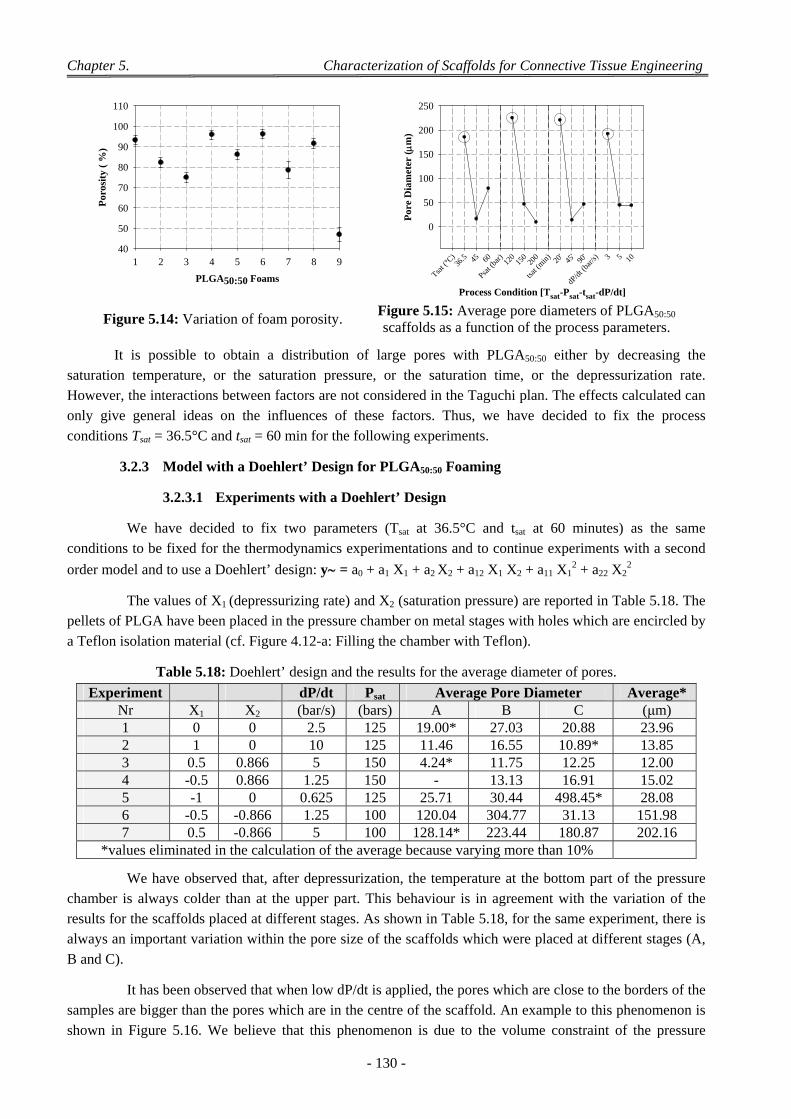
Chapter 5. Characterization of Scaffolds for Connective Tissue Engineering
- 130 -
PLGA50:50 Foam Porosity
PLGA50:50 Foams
1 2 3 4 5 6 7 8 9
Por
osit
y (
%)
40
50
60
70
80
90
100
110
Optimum Parameters
Process Condition [Tsat-Psat-tsat-dP/dt]
Tsat (
°C)
36.5 45 60
Psat (
bar)
120
150
200
tsat (
min)
20'
45'
90'
dP/dt
(bar/
s) 3 5 10
Por
e D
iam
eter
(m
)
0
50
100
150
200
250
Figure 5.14: Variation of foam porosity. Figure 5.15: Average pore diameters of PLGA50:50 scaffolds as a function of the process parameters.
It is possible to obtain a distribution of large pores with PLGA50:50 either by decreasing the saturation temperature, or the saturation pressure, or the saturation time, or the depressurization rate. However, the interactions between factors are not considered in the Taguchi plan. The effects calculated can only give general ideas on the influences of these factors. Thus, we have decided to fix the process
conditions Tsat = 36.5°C and tsat = 60 min for the following experiments.
3.2.3 Model with a Doehlert’ Design for PLGA50:50 Foaming
3.2.3.1 Experiments with a Doehlert’ Design
We have decided to fix two parameters (Tsat at 36.5°C and tsat at 60 minutes) as the same conditions to be fixed for the thermodynamics experimentations and to continue experiments with a second
order model and to use a Doehlert’ design: y = a0 + a1 X1 + a2 X2 + a12 X1 X2 + a11 X12 + a22 X2
2
The values of X1 (depressurizing rate) and X2 (saturation pressure) are reported in Table 5.18. The pellets of PLGA have been placed in the pressure chamber on metal stages with holes which are encircled by
a Teflon isolation material (cf. Figure 4.12-a: Filling the chamber with Teflon).
Table 5.18: Doehlert’ design and the results for the average diameter of pores.
Experiment dP/dt Psat Average Pore Diameter Average* Nr X1 X2 (bar/s) (bars) A B C (μm) 1 0 0 2.5 125 19.00* 27.03 20.88 23.96 2 1 0 10 125 11.46 16.55 10.89* 13.85 3 0.5 0.866 5 150 4.24* 11.75 12.25 12.00 4 -0.5 0.866 1.25 150 - 13.13 16.91 15.02 5 -1 0 0.625 125 25.71 30.44 498.45* 28.08 6 -0.5 -0.866 1.25 100 120.04 304.77 31.13 151.98 7 0.5 -0.866 5 100 128.14* 223.44 180.87 202.16
*values eliminated in the calculation of the average because varying more than 10%
We have observed that, after depressurization, the temperature at the bottom part of the pressure chamber is always colder than at the upper part. This behaviour is in agreement with the variation of the results for the scaffolds placed at different stages. As shown in Table 5.18, for the same experiment, there is always an important variation within the pore size of the scaffolds which were placed at different stages (A,
B and C).
It has been observed that when low dP/dt is applied, the pores which are close to the borders of the samples are bigger than the pores which are in the centre of the scaffold. An example to this phenomenon is shown in Figure 5.16. We believe that this phenomenon is due to the volume constraint of the pressure
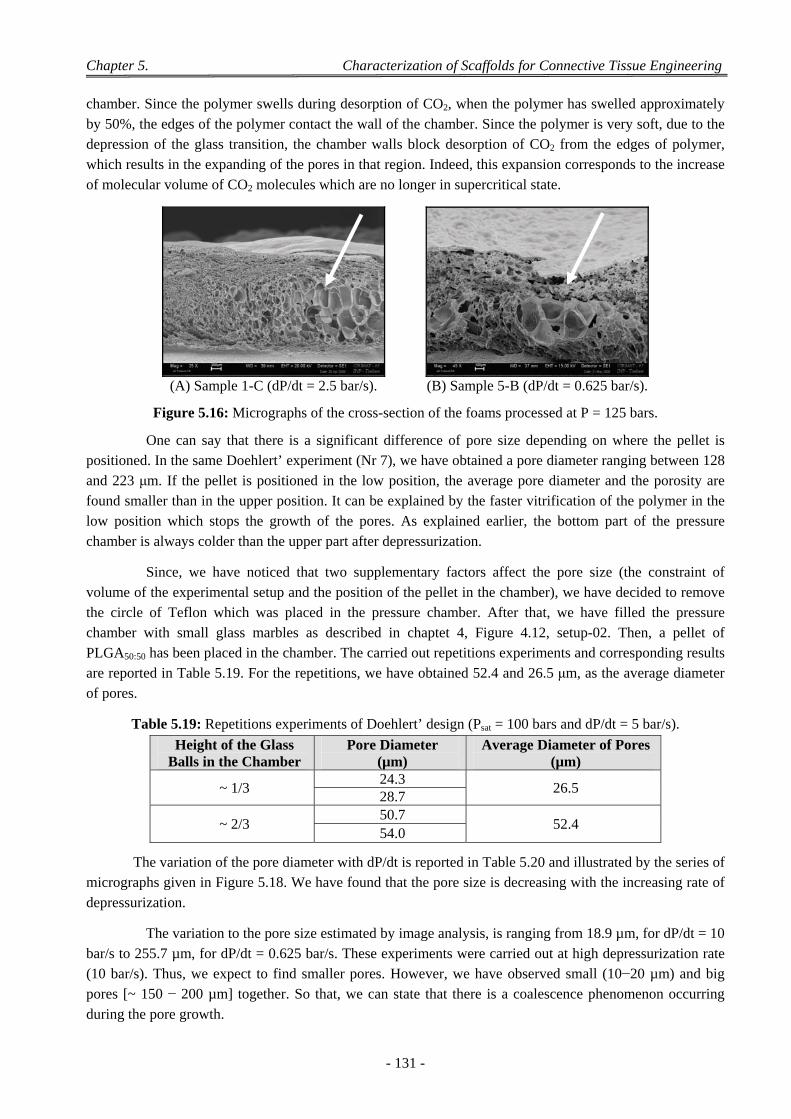
Chapter 5. Characterization of Scaffolds for Connective Tissue Engineering
- 131 -
chamber. Since the polymer swells during desorption of CO2, when the polymer has swelled approximately by 50%, the edges of the polymer contact the wall of the chamber. Since the polymer is very soft, due to the depression of the glass transition, the chamber walls block desorption of CO2 from the edges of polymer, which results in the expanding of the pores in that region. Indeed, this expansion corresponds to the increase
of molecular volume of CO2 molecules which are no longer in supercritical state.
(A) Sample 1-C (dP/dt = 2.5 bar/s). (B) Sample 5-B (dP/dt = 0.625 bar/s).
Figure 5.16: Micrographs of the cross-section of the foams processed at P = 125 bars.
One can say that there is a significant difference of pore size depending on where the pellet is positioned. In the same Doehlert’ experiment (Nr 7), we have obtained a pore diameter ranging between 128 and 223 μm. If the pellet is positioned in the low position, the average pore diameter and the porosity are found smaller than in the upper position. It can be explained by the faster vitrification of the polymer in the low position which stops the growth of the pores. As explained earlier, the bottom part of the pressure
chamber is always colder than the upper part after depressurization.
Since, we have noticed that two supplementary factors affect the pore size (the constraint of volume of the experimental setup and the position of the pellet in the chamber), we have decided to remove the circle of Teflon which was placed in the pressure chamber. After that, we have filled the pressure chamber with small glass marbles as described in chaptet 4, Figure 4.12, setup-02. Then, a pellet of PLGA50:50 has been placed in the chamber. The carried out repetitions experiments and corresponding results are reported in Table 5.19. For the repetitions, we have obtained 52.4 and 26.5 μm, as the average diameter of pores.
Table 5.19: Repetitions experiments of Doehlert’ design (Psat = 100 bars and dP/dt = 5 bar/s).
Height of the Glass Balls in the Chamber
Pore Diameter (µm)
Average Diameter of Pores (µm)
~ 1/3 24.3
26.5 28.7
~ 2/3 50.7
52.4 54.0
The variation of the pore diameter with dP/dt is reported in Table 5.20 and illustrated by the series of micrographs given in Figure 5.18. We have found that the pore size is decreasing with the increasing rate of
depressurization.
The variation to the pore size estimated by image analysis, is ranging from 18.9 µm, for dP/dt = 10 bar/s to 255.7 µm, for dP/dt = 0.625 bar/s. These experiments were carried out at high depressurization rate (10 bar/s). Thus, we expect to find smaller pores. However, we have observed small (10−20 µm) and big pores [~ 150 − 200 µm] together. So that, we can state that there is a coalescence phenomenon occurring
during the pore growth.
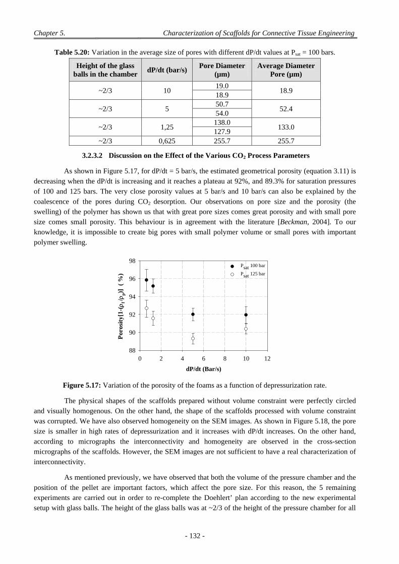
Chapter 5. Characterization of Scaffolds for Connective Tissue Engineering
- 132 -
Table 5.20: Variation in the average size of pores with different dP/dt values at Psat = 100 bars.
Height of the glass balls in the chamber
dP/dt (bar/s) Pore Diameter
(µm) Average Diameter
Pore (µm)
~2/3 10 19.0
18.9 18.9
~2/3 5 50.7
52.4 54.0
~2/3 1,25 138.0
133.0 127.9
~2/3 0,625 255.7 255.7
3.2.3.2 Discussion on the Effect of the Various CO2 Process Parameters
As shown in Figure 5.17, for dP/dt = 5 bar/s, the estimated geometrical porosity (equation 3.11) is decreasing when the dP/dt is increasing and it reaches a plateau at 92%, and 89.3% for saturation pressures of 100 and 125 bars. The very close porosity values at 5 bar/s and 10 bar/s can also be explained by the coalescence of the pores during CO2 desorption. Our observations on pore size and the porosity (the swelling) of the polymer has shown us that with great pore sizes comes great porosity and with small pore size comes small porosity. This behaviour is in agreement with the literature [Beckman, 2004]. To our knowledge, it is impossible to create big pores with small polymer volume or small pores with important
polymer swelling.
PLGA50:50 Porosity Variation
dP/dt (Bar/s)
0 2 4 6 8 10 12
Por
osit
y[1-
( f /
p)]
( %
)
88
90
92
94
96
98Psat 100 bar
Psat 125 bar
Figure 5.17: Variation of the porosity of the foams as a function of depressurization rate.
The physical shapes of the scaffolds prepared without volume constraint were perfectly circled and visually homogenous. On the other hand, the shape of the scaffolds processed with volume constraint was corrupted. We have also observed homogeneity on the SEM images. As shown in Figure 5.18, the pore size is smaller in high rates of depressurization and it increases with dP/dt increases. On the other hand, according to micrographs the interconnectivity and homogeneity are observed in the cross-section micrographs of the scaffolds. However, the SEM images are not sufficient to have a real characterization of
interconnectivity.
As mentioned previously, we have observed that both the volume of the pressure chamber and the position of the pellet are important factors, which affect the pore size. For this reason, the 5 remaining experiments are carried out in order to re-complete the Doehlert’ plan according to the new experimental setup with glass balls. The height of the glass balls was at ~2/3 of the height of the pressure chamber for all
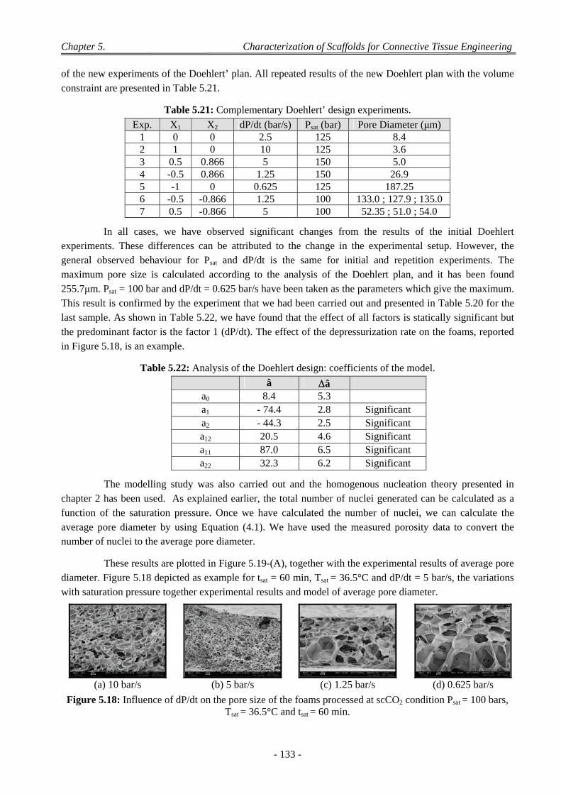
Chapter 5. Characterization of Scaffolds for Connective Tissue Engineering
- 133 -
of the new experiments of the Doehlert’ plan. All repeated results of the new Doehlert plan with the volume
constraint are presented in Table 5.21.
Table 5.21: Complementary Doehlert’ design experiments.
Exp. X1 X2 dP/dt (bar/s) Psat (bar) Pore Diameter (μm) 1 0 0 2.5 125 8.4 2 1 0 10 125 3.6 3 0.5 0.866 5 150 5.0 4 -0.5 0.866 1.25 150 26.9 5 -1 0 0.625 125 187.25 6 -0.5 -0.866 1.25 100 133.0 ; 127.9 ; 135.0 7 0.5 -0.866 5 100 52.35 ; 51.0 ; 54.0
In all cases, we have observed significant changes from the results of the initial Doehlert experiments. These differences can be attributed to the change in the experimental setup. However, the general observed behaviour for Psat and dP/dt is the same for initial and repetition experiments. The maximum pore size is calculated according to the analysis of the Doehlert plan, and it has been found 255.7μm. Psat = 100 bar and dP/dt = 0.625 bar/s have been taken as the parameters which give the maximum. This result is confirmed by the experiment that we had been carried out and presented in Table 5.20 for the last sample. As shown in Table 5.22, we have found that the effect of all factors is statically significant but the predominant factor is the factor 1 (dP/dt). The effect of the depressurization rate on the foams, reported
in Figure 5.18, is an example.
Table 5.22: Analysis of the Doehlert design: coefficients of the model.
â â a0 8.4 5.3 a1 - 74.4 2.8 Significant a2 - 44.3 2.5 Significant a12 20.5 4.6 Significant a11 87.0 6.5 Significant a22 32.3 6.2 Significant
The modelling study was also carried out and the homogenous nucleation theory presented in chapter 2 has been used. As explained earlier, the total number of nuclei generated can be calculated as a function of the saturation pressure. Once we have calculated the number of nuclei, we can calculate the average pore diameter by using Equation (4.1). We have used the measured porosity data to convert the number of nuclei to the average pore diameter.
These results are plotted in Figure 5.19-(A), together with the experimental results of average pore diameter. Figure 5.18 depicted as example for tsat = 60 min, Tsat = 36.5°C and dP/dt = 5 bar/s, the variations with saturation pressure together experimental results and model of average pore diameter.
(a) 10 bar/s (b) 5 bar/s (c) 1.25 bar/s (d) 0.625 bar/s
Figure 5.18: Influence of dP/dt on the pore size of the foams processed at scCO2 condition Psat = 100 bars, Tsat = 36.5°C and tsat = 60 min.
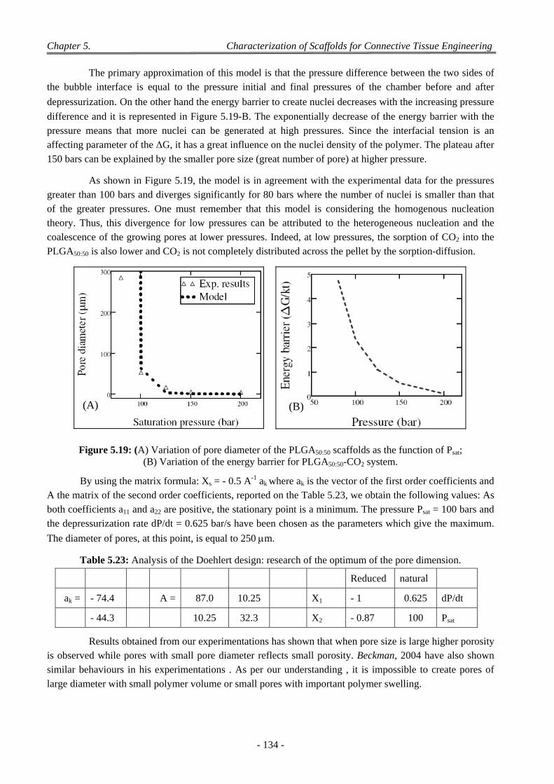
Chapter 5. Characterization of Scaffolds for Connective Tissue Engineering
- 134 -
The primary approximation of this model is that the pressure difference between the two sides of the bubble interface is equal to the pressure initial and final pressures of the chamber before and after
depressurization. On the other hand the energy barrier to create nuclei decreases with the increasing pressure
difference and it is represented in Figure 5.19-B. The exponentially decrease of the energy barrier with the pressure means that more nuclei can be generated at high pressures. Since the interfacial tension is an affecting parameter of the ΔG, it has a great influence on the nuclei density of the polymer. The plateau after
150 bars can be explained by the smaller pore size (great number of pore) at higher pressure.
As shown in Figure 5.19, the model is in agreement with the experimental data for the pressures greater than 100 bars and diverges significantly for 80 bars where the number of nuclei is smaller than that of the greater pressures. One must remember that this model is considering the homogenous nucleation theory. Thus, this divergence for low pressures can be attributed to the heterogeneous nucleation and the coalescence of the growing pores at lower pressures. Indeed, at low pressures, the sorption of CO2 into the
PLGA50:50 is also lower and CO2 is not completely distributed across the pellet by the sorption-diffusion.
Figure 5.19: (A) Variation of pore diameter of the PLGA50:50 scaffolds as the function of Psat; (B) Variation of the energy barrier for PLGA50:50-CO2 system.
By using the matrix formula: Xs = - 0.5 A-1 ak where ak is the vector of the first order coefficients and A the matrix of the second order coefficients, reported on the Table 5.23, we obtain the following values: As both coefficients a11 and a22 are positive, the stationary point is a minimum. The pressure Psat = 100 bars and the depressurization rate dP/dt = 0.625 bar/s have been chosen as the parameters which give the maximum.
The diameter of pores, at this point, is equal to 250 m.
Table 5.23: Analysis of the Doehlert design: research of the optimum of the pore dimension.
Reduced natural
ak = - 74.4 A = 87.0 10.25 X1 - 1 0.625 dP/dt
- 44.3 10.25 32.3 X2 - 0.87 100 Psat
Results obtained from our experimentations has shown that when pore size is large higher porosity is observed while pores with small pore diameter reflects small porosity. Beckman, 2004 have also shown similar behaviours in his experimentations . As per our understanding , it is impossible to create pores of
large diameter with small polymer volume or small pores with important polymer swelling.
(A) (B)
Chapter 5. Characterization of Scaffolds for Connective Tissue Engineering
- 135 -
4 Factors Affecting on Pores Size and Porosity
4.1 Effect of the Polymer Composition
The Hildebrand’s solubility parameters can be separated into three Hansen’ components by the
relationship given in following equation 5.1.
δt2= δd
2+δp2 +δH
2 (5. 1)
where δt is the Hildebrand’s parameter (cf.Table 5.24), δd is the dispersive component, δp is the polar
component and δH is the hydrogen bond component [Risanen, 2010; Schenderlein et al., 2004].
In the case of supercritical fluids the relationship linking the Hildebrand’ parameter to the Pc
critical pressure is the following [Li. and Perrut, 1991].
= 1,25 Pc /l (5.2)
where and l are corresponding to the density to the fluid in their supercritical and liquid state
respectively. ScCO2 is a apolar fluid (14,3 < < 18,4).
Table 5.24: Hidebrand’ and Hansen’ parameters of the PLA and the PGA in (MPa)1/2.
d p H t t*PLA 18.5 9.7 6.0 21.7 20.2
PGA 11.7 6.21 12.5 18.2 24.8 *Calculations with the Small’ group contribution method.
Normally both amorphous PLAs and PLGAs produce scaffolds of higher porosity and large pore diameters. Increase in the LA content in the PLGA co-polymer increases the solubility of CO2 in the polymers. The solubility of CO2 is always higher in all poly D,L-lactides than poly(lactides co-glycolide). The extra apolar group in polylactide acid is responsible for higher solubility in the polylactide which eventually generates highly porous foams depending upon the process conditions. According to Liu and Tomasko [2007b] the extra apolar group which is not present in glycolic acid, leades to two opposite and different phenomenon. The effect of CO2 interaction with the carbonyl group of the polymer is decreased due to the apolar group first and secondly, more available free volume for CO2 to solubilise is created. Kazarian et al. [1996b] has also found that the interaction of CO2 with polymers can also be explained by
the CO2 behaviour as a Lewis acid, an electron pair acceptor.
LA/GA ratio of a PLGA co-polymer is an important parameter to control the pore diameter in a foaming process. Foaming of PLGA with different LA and GA contents, has given different results. In our study, with the same foaming conditions (Psat, Tsat, tsat, dT/dt), we have experienced different pore size behaviours when processed with rapid or slow depressurizations. Secondly, low pores size can be due to high saturation pressure and low saturation temperature with comparison to the Tg of both polymers (cf.
Table 5.5).
4.2 Effect of Depressurization Rates
For low depressurization rates (0.625 to 1.25 bar/s), when the lactic acid content increases in PLGA, the pore size increases as well. This behaviour can be attributed to the greater capacity of solubilized CO2 inside the polymer with the increasing amount of LA. Actually, one can expect that since the CO2 concentration is greater in a high lactic acid containing PLGA, the nucleation rate must be greater (which means lower pore size). However, even if the number of pores is determined by the saturation period and the
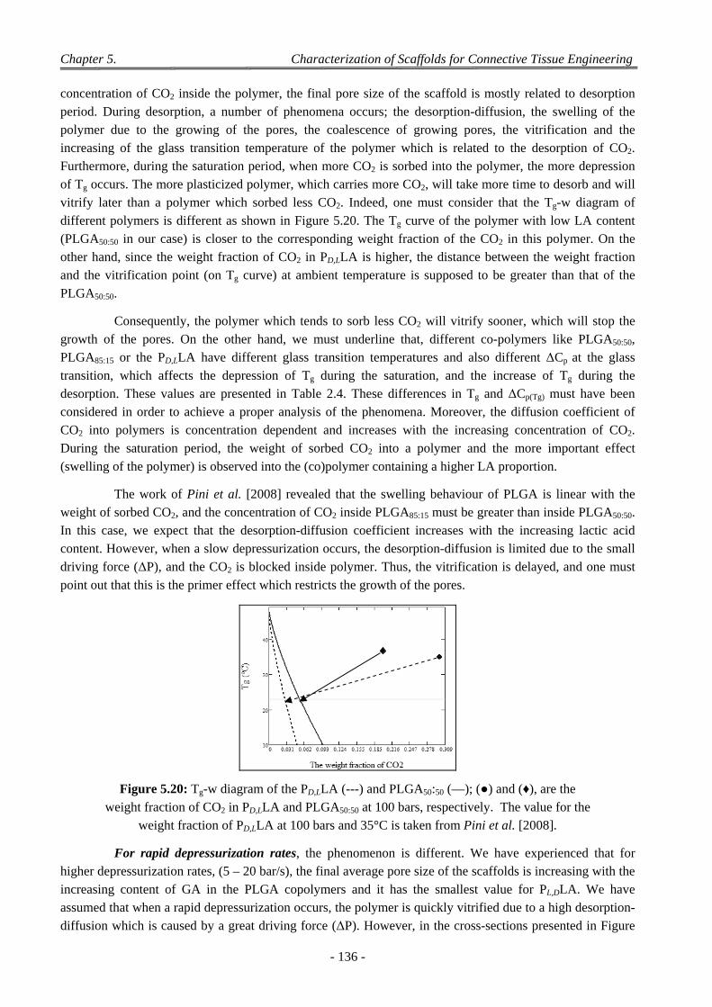
Chapter 5. Characterization of Scaffolds for Connective Tissue Engineering
- 136 -
concentration of CO2 inside the polymer, the final pore size of the scaffold is mostly related to desorption period. During desorption, a number of phenomena occurs; the desorption-diffusion, the swelling of the polymer due to the growing of the pores, the coalescence of growing pores, the vitrification and the increasing of the glass transition temperature of the polymer which is related to the desorption of CO2. Furthermore, during the saturation period, when more CO2 is sorbed into the polymer, the more depression of Tg occurs. The more plasticized polymer, which carries more CO2, will take more time to desorb and will vitrify later than a polymer which sorbed less CO2. Indeed, one must consider that the Tg-w diagram of different polymers is different as shown in Figure 5.20. The Tg curve of the polymer with low LA content (PLGA50:50 in our case) is closer to the corresponding weight fraction of the CO2 in this polymer. On the other hand, since the weight fraction of CO2 in PD,LLA is higher, the distance between the weight fraction and the vitrification point (on Tg curve) at ambient temperature is supposed to be greater than that of the
PLGA50:50.
Consequently, the polymer which tends to sorb less CO2 will vitrify sooner, which will stop the growth of the pores. On the other hand, we must underline that, different co-polymers like PLGA50:50, PLGA85:15 or the PD,LLA have different glass transition temperatures and also different ΔCp at the glass transition, which affects the depression of Tg during the saturation, and the increase of Tg during the desorption. These values are presented in Table 2.4. These differences in Tg and ΔCp(Tg) must have been considered in order to achieve a proper analysis of the phenomena. Moreover, the diffusion coefficient of CO2 into polymers is concentration dependent and increases with the increasing concentration of CO2. During the saturation period, the weight of sorbed CO2 into a polymer and the more important effect
(swelling of the polymer) is observed into the (co)polymer containing a higher LA proportion.
The work of Pini et al. [2008] revealed that the swelling behaviour of PLGA is linear with the weight of sorbed CO2, and the concentration of CO2 inside PLGA85:15 must be greater than inside PLGA50:50. In this case, we expect that the desorption-diffusion coefficient increases with the increasing lactic acid content. However, when a slow depressurization occurs, the desorption-diffusion is limited due to the small driving force (ΔP), and the CO2 is blocked inside polymer. Thus, the vitrification is delayed, and one must
point out that this is the primer effect which restricts the growth of the pores.
Figure 5.20: Tg-w diagram of the PD,LLA (---) and PLGA50:50 (—); (●) and (♦), are the weight fraction of CO2 in PD,LLA and PLGA50:50 at 100 bars, respectively. The value for the
weight fraction of PD,LLA at 100 bars and 35°C is taken from Pini et al. [2008].
For rapid depressurization rates, the phenomenon is different. We have experienced that for higher depressurization rates, (5 – 20 bar/s), the final average pore size of the scaffolds is increasing with the increasing content of GA in the PLGA copolymers and it has the smallest value for PL,DLA. We have assumed that when a rapid depressurization occurs, the polymer is quickly vitrified due to a high desorption-diffusion which is caused by a great driving force (ΔP). However, in the cross-sections presented in Figure
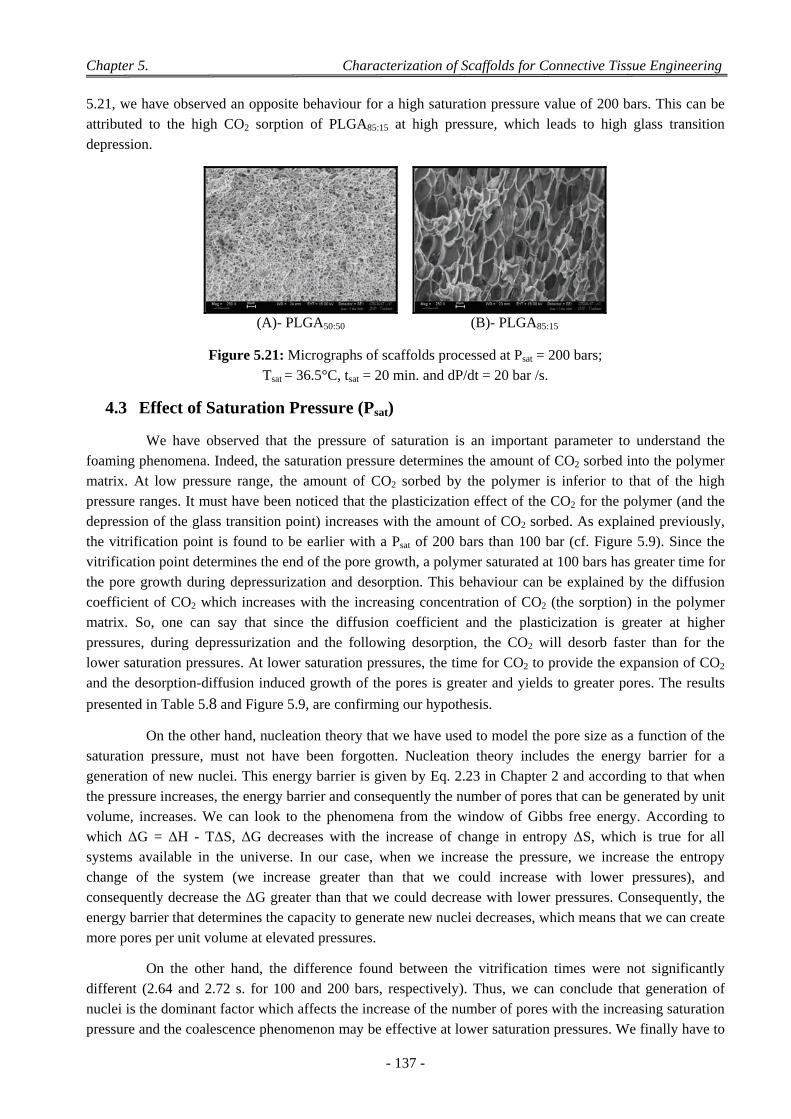
Chapter 5. Characterization of Scaffolds for Connective Tissue Engineering
- 137 -
5.21, we have observed an opposite behaviour for a high saturation pressure value of 200 bars. This can be attributed to the high CO2 sorption of PLGA85:15 at high pressure, which leads to high glass transition
depression.
(A)- PLGA50:50 (B)- PLGA85:15
Figure 5.21: Micrographs of scaffolds processed at Psat = 200 bars; Tsat = 36.5°C, tsat = 20 min. and dP/dt = 20 bar /s.
4.3 Effect of Saturation Pressure (Psat)
We have observed that the pressure of saturation is an important parameter to understand the foaming phenomena. Indeed, the saturation pressure determines the amount of CO2 sorbed into the polymer matrix. At low pressure range, the amount of CO2 sorbed by the polymer is inferior to that of the high pressure ranges. It must have been noticed that the plasticization effect of the CO2 for the polymer (and the depression of the glass transition point) increases with the amount of CO2 sorbed. As explained previously, the vitrification point is found to be earlier with a Psat of 200 bars than 100 bar (cf. Figure 5.9). Since the vitrification point determines the end of the pore growth, a polymer saturated at 100 bars has greater time for the pore growth during depressurization and desorption. This behaviour can be explained by the diffusion coefficient of CO2 which increases with the increasing concentration of CO2 (the sorption) in the polymer matrix. So, one can say that since the diffusion coefficient and the plasticization is greater at higher pressures, during depressurization and the following desorption, the CO2 will desorb faster than for the lower saturation pressures. At lower saturation pressures, the time for CO2 to provide the expansion of CO2 and the desorption-diffusion induced growth of the pores is greater and yields to greater pores. The results
presented in Table 5.8 and Figure 5.9, are confirming our hypothesis.
On the other hand, nucleation theory that we have used to model the pore size as a function of the saturation pressure, must not have been forgotten. Nucleation theory includes the energy barrier for a generation of new nuclei. This energy barrier is given by Eq. 2.23 in Chapter 2 and according to that when the pressure increases, the energy barrier and consequently the number of pores that can be generated by unit volume, increases. We can look to the phenomena from the window of Gibbs free energy. According to which ΔG = ΔH - TΔS, ΔG decreases with the increase of change in entropy ΔS, which is true for all systems available in the universe. In our case, when we increase the pressure, we increase the entropy change of the system (we increase greater than that we could increase with lower pressures), and consequently decrease the ΔG greater than that we could decrease with lower pressures. Consequently, the energy barrier that determines the capacity to generate new nuclei decreases, which means that we can create
more pores per unit volume at elevated pressures.
On the other hand, the difference found between the vitrification times were not significantly different (2.64 and 2.72 s. for 100 and 200 bars, respectively). Thus, we can conclude that generation of nuclei is the dominant factor which affects the increase of the number of pores with the increasing saturation pressure and the coalescence phenomenon may be effective at lower saturation pressures. We finally have to
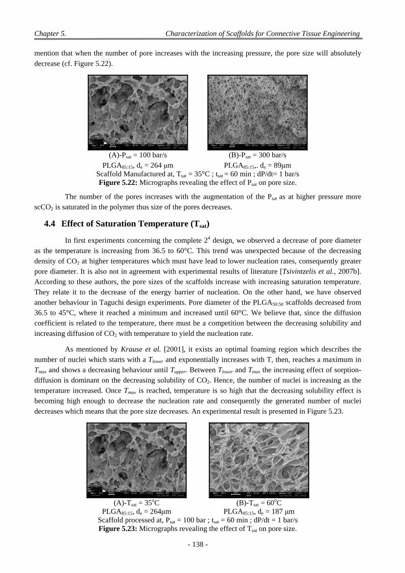
Chapter 5. Characterization of Scaffolds for Connective Tissue Engineering
- 138 -
mention that when the number of pore increases with the increasing pressure, the pore size will absolutely
decrease (cf. Figure 5.22).
(A)-Psat = 100 bar/s (B)-Psat = 300 bar/s
PLGA85:15, de = 264 μm PLGA85:15,. de = 89μm Scaffold Manufactured at, Tsat = 35°C ; tsat = 60 min ; dP/dt= 1 bar/s Figure 5.22: Micrographs revealing the effect of Psat on pore size.
The number of the pores increases with the augmentation of the Psat as at higher pressure more scCO2 is saturated in the polymer thus size of the pores decreases.
4.4 Effect of Saturation Temperature (Tsat)
In first experiments concerning the complete 24 design, we observed a decrease of pore diameter as the temperature is increasing from 36.5 to 60°C. This trend was unexpected because of the decreasing density of CO2 at higher temperatures which must have lead to lower nucleation rates, consequently greater pore diameter. It is also not in agreement with experimental results of literature [Tsivintzelis et al., 2007b]. According to these authors, the pore sizes of the scaffolds increase with increasing saturation temperature. They relate it to the decrease of the energy barrier of nucleation. On the other hand, we have observed another behaviour in Taguchi design experiments. Pore diameter of the PLGA50:50 scaffolds decreased from 36.5 to 45°C, where it reached a minimum and increased until 60°C. We believe that, since the diffusion coefficient is related to the temperature, there must be a competition between the decreasing solubility and
increasing diffusion of CO2 with temperature to yield the nucleation rate.
As mentioned by Krause et al. [2001], it exists an optimal foaming region which describes the number of nuclei which starts with a Tlower and exponentially increases with T, then, reaches a maximum in Tmax and shows a decreasing behaviour until Tupper. Between Tlower and Tmax the increasing effect of sorption-diffusion is dominant on the decreasing solubility of CO2. Hence, the number of nuclei is increasing as the temperature increased. Once Tmax is reached, temperature is so high that the decreasing solubility effect is becoming high enough to decrease the nucleation rate and consequently the generated number of nuclei
decreases which means that the pore size decreases. An experimental result is presented in Figure 5.23.
(A)-Tsat = 35oC (B)-Tsat = 60oC
PLGA85:15, de = 264μm PLGA85:15, de = 187 μm Scaffold processed at, Psat = 100 bar ; tsat = 60 min ; dP/dt = 1 bar/s Figure 5.23: Micrographs revealing the effect of Tsat on pore size.
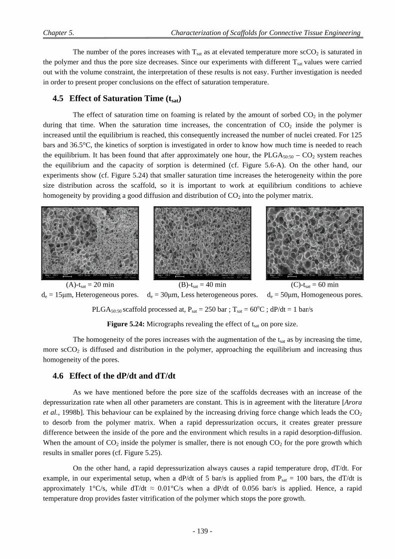
Chapter 5. Characterization of Scaffolds for Connective Tissue Engineering
- 139 -
The number of the pores increases with Tsat as at elevated temperature more scCO2 is saturated in the polymer and thus the pore size decreases. Since our experiments with different Tsat values were carried out with the volume constraint, the interpretation of these results is not easy. Further investigation is needed
in order to present proper conclusions on the effect of saturation temperature.
4.5 Effect of Saturation Time (tsat)
The effect of saturation time on foaming is related by the amount of sorbed CO2 in the polymer during that time. When the saturation time increases, the concentration of CO2 inside the polymer is increased until the equilibrium is reached, this consequently increased the number of nuclei created. For 125 bars and 36.5°C, the kinetics of sorption is investigated in order to know how much time is needed to reach the equilibrium. It has been found that after approximately one hour, the PLGA50:50 – CO2 system reaches the equilibrium and the capacity of sorption is determined (cf. Figure 5.6-A). On the other hand, our experiments show (cf. Figure 5.24) that smaller saturation time increases the heterogeneity within the pore size distribution across the scaffold, so it is important to work at equilibrium conditions to achieve
homogeneity by providing a good diffusion and distribution of CO2 into the polymer matrix.
(A)-tsat = 20 min (B)-tsat = 40 min (C)-tsat = 60 min
de = 15μm, Heterogeneous pores. de = 30μm, Less heterogeneous pores. de = 50μm, Homogeneous pores.
PLGA50:50 scaffold processed at, Psat = 250 bar ; Tsat = 60oC ; dP/dt = 1 bar/s
Figure 5.24: Micrographs revealing the effect of tsat on pore size.
The homogeneity of the pores increases with the augmentation of the tsat as by increasing the time, more scCO2 is diffused and distribution in the polymer, approaching the equilibrium and increasing thus
homogeneity of the pores.
4.6 Effect of the dP/dt and dT/dt
As we have mentioned before the pore size of the scaffolds decreases with an increase of the depressurization rate when all other parameters are constant. This is in agreement with the literature [Arora et al., 1998b]. This behaviour can be explained by the increasing driving force change which leads the CO2 to desorb from the polymer matrix. When a rapid depressurization occurs, it creates greater pressure difference between the inside of the pore and the environment which results in a rapid desorption-diffusion. When the amount of CO2 inside the polymer is smaller, there is not enough CO2 for the pore growth which
results in smaller pores (cf. Figure 5.25).
On the other hand, a rapid depressurization always causes a rapid temperature drop, dT/dt. For example, in our experimental setup, when a dP/dt of 5 bar/s is applied from Psat = 100 bars, the dT/dt is approximately 1°C/s, while dT/dt ≈ 0.01°C/s when a dP/dt of 0.056 bar/s is applied. Hence, a rapid
temperature drop provides faster vitrification of the polymer which stops the pore growth.
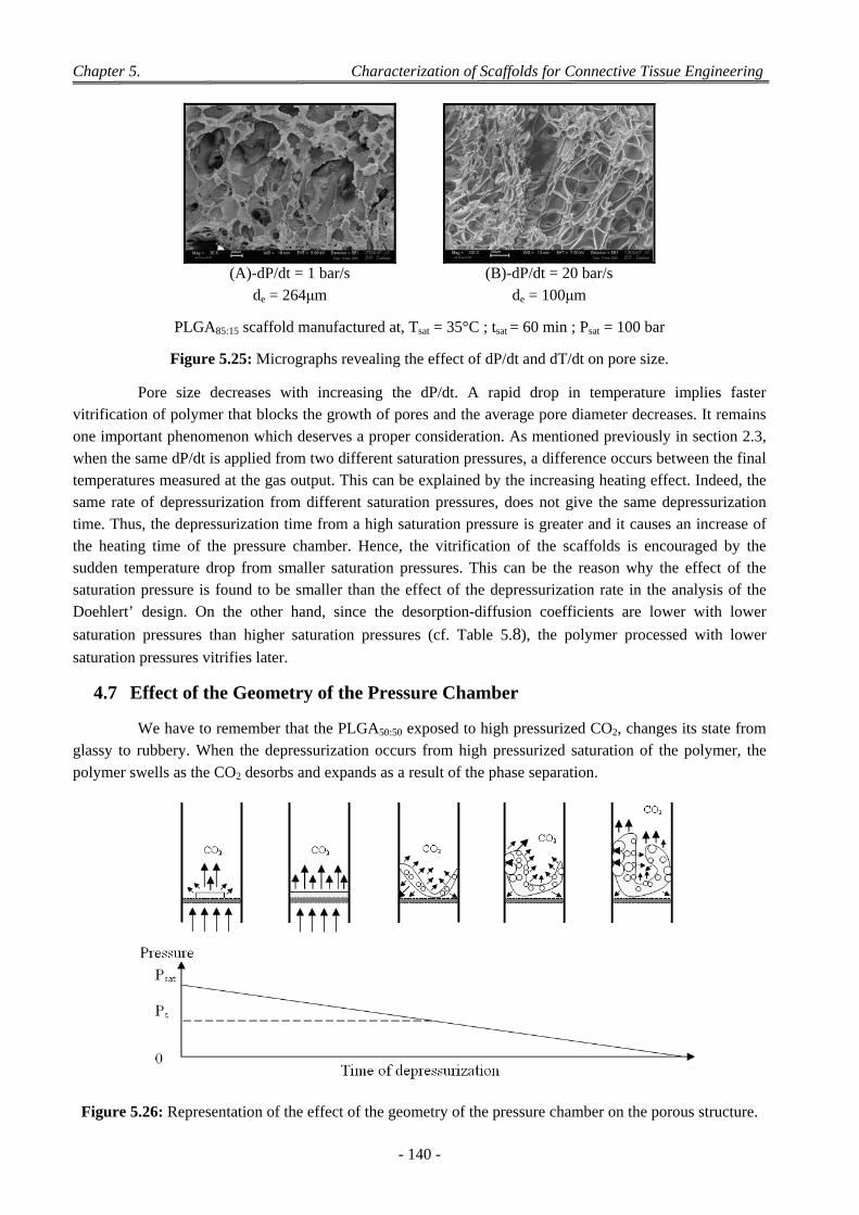
Chapter 5. Characterization of Scaffolds for Connective Tissue Engineering
- 140 -
(A)-dP/dt = 1 bar/s (B)-dP/dt = 20 bar/s
de = 264μm de = 100μm
PLGA85:15 scaffold manufactured at, Tsat = 35°C ; tsat = 60 min ; Psat = 100 bar
Figure 5.25: Micrographs revealing the effect of dP/dt and dT/dt on pore size.
Pore size decreases with increasing the dP/dt. A rapid drop in temperature implies faster vitrification of polymer that blocks the growth of pores and the average pore diameter decreases. It remains one important phenomenon which deserves a proper consideration. As mentioned previously in section 2.3, when the same dP/dt is applied from two different saturation pressures, a difference occurs between the final temperatures measured at the gas output. This can be explained by the increasing heating effect. Indeed, the same rate of depressurization from different saturation pressures, does not give the same depressurization time. Thus, the depressurization time from a high saturation pressure is greater and it causes an increase of the heating time of the pressure chamber. Hence, the vitrification of the scaffolds is encouraged by the sudden temperature drop from smaller saturation pressures. This can be the reason why the effect of the saturation pressure is found to be smaller than the effect of the depressurization rate in the analysis of the Doehlert’ design. On the other hand, since the desorption-diffusion coefficients are lower with lower
saturation pressures than higher saturation pressures (cf. Table 5.8), the polymer processed with lower
saturation pressures vitrifies later.
4.7 Effect of the Geometry of the Pressure Chamber
We have to remember that the PLGA50:50 exposed to high pressurized CO2, changes its state from glassy to rubbery. When the depressurization occurs from high pressurized saturation of the polymer, the
polymer swells as the CO2 desorbs and expands as a result of the phase separation.
Figure 5.26: Representation of the effect of the geometry of the pressure chamber on the porous structure.
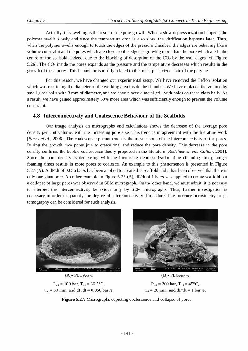
Chapter 5. Characterization of Scaffolds for Connective Tissue Engineering
- 141 -
Actually, this swelling is the result of the pore growth. When a slow depressurization happens, the polymer swells slowly and since the temperature drop is also slow, the vitrification happens later. Thus, when the polymer swells enough to touch the edges of the pressure chamber, the edges are behaving like a volume constraint and the pores which are closer to the edges is growing more than the pore which are in the centre of the scaffold, indeed, due to the blocking of desorption of the CO2 by the wall edges (cf. Figure 5.26). The CO2 inside the pores expands as the pressure and the temperature decreases which results in the
growth of these pores. This behaviour is mostly related to the much plasticized state of the polymer.
For this reason, we have changed our experimental setup. We have removed the Teflon isolation which was restricting the diameter of the working area inside the chamber. We have replaced the volume by small glass balls with 3 mm of diameter, and we have placed a metal grill with holes on these glass balls. As a result, we have gained approximately 50% more area which was sufficiently enough to prevent the volume
constraint.
4.8 Interconnectivity and Coalescence Behaviour of the Scaffolds
Our image analysis on micrographs and calculations shows the decrease of the average pore density per unit volume, with the increasing pore size. This trend is in agreement with the literature work [Barry et al., 2006]. The coalescence phenomenon is the master bone of the interconnectivity of the pores. During the growth, two pores join to create one, and reduce the pore density. This decrease in the pore density confirms the bubble coalescence theory proposed in the literature [Rodeheaver and Colton, 2001]. Since the pore density is decreasing with the increasing depressurization time (foaming time), longer foaming times results in more pores to coalesce. An example to this phenomenon is presented in Figure 5.27-(A). A dP/dt of 0.056 bar/s has been applied to create this scaffold and it has been observed that there is only one giant pore. An other example in Figure 5.27-(B), dP/dt of 1 bar/s was applied to create scaffold but a collapse of large pores was observed in SEM micrograph. On the other hand, we must admit, it is not easy to interpret the interconnectivity behaviour only by SEM micrographs. Thus, further investigation is necessary in order to quantify the degree of interconnectivity. Procedures like mercury porosimetry or µ-
tomography can be considered for such analysis.
(A)- PLGA50:50 (B)- PLGA85:15
Psat = 100 bar, Tsat = 36.5°C, tsat = 60 min. and dP/dt = 0.056 bar /s.
Psat = 200 bar, Tsat = 45°C, tsat = 20 min. and dP/dt = 1 bar /s.
Figure 5.27: Micrographs depicting coalescence and collapse of pores.
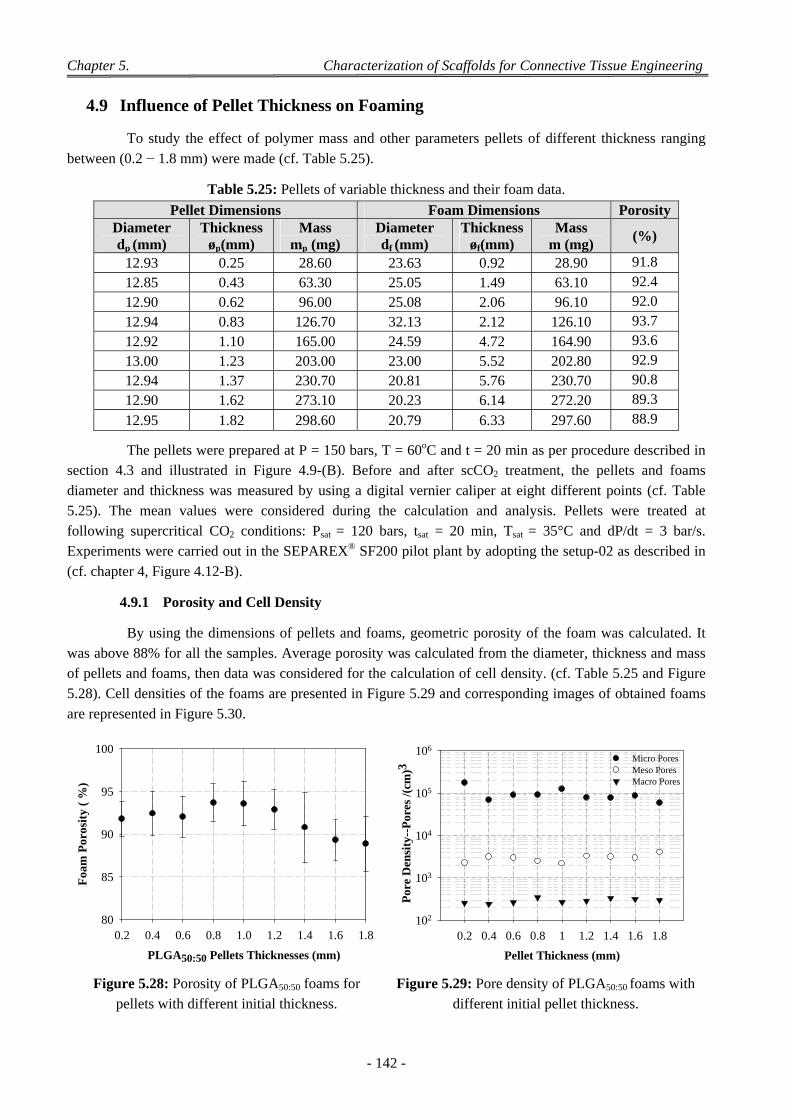
Chapter 5. Characterization of Scaffolds for Connective Tissue Engineering
- 142 -
4.9 Influence of Pellet Thickness on Foaming
To study the effect of polymer mass and other parameters pellets of different thickness ranging
between (0.2 − 1.8 mm) were made (cf. Table 5.25).
Table 5.25: Pellets of variable thickness and their foam data.
Pellet Dimensions Foam Dimensions Porosity Diameter dp (mm)
Thickness øp(mm)
Mass mp (mg)
Diameter df (mm)
Thickness øf(mm)
Mass m (mg)
(%)
12.93 0.25 28.60 23.63 0.92 28.90 91.8
12.85 0.43 63.30 25.05 1.49 63.10 92.4
12.90 0.62 96.00 25.08 2.06 96.10 92.0
12.94 0.83 126.70 32.13 2.12 126.10 93.7
12.92 1.10 165.00 24.59 4.72 164.90 93.6
13.00 1.23 203.00 23.00 5.52 202.80 92.9
12.94 1.37 230.70 20.81 5.76 230.70 90.8
12.90 1.62 273.10 20.23 6.14 272.20 89.3
12.95 1.82 298.60 20.79 6.33 297.60 88.9
The pellets were prepared at P = 150 bars, T = 60oC and t = 20 min as per procedure described in section 4.3 and illustrated in Figure 4.9-(B). Before and after scCO2 treatment, the pellets and foams diameter and thickness was measured by using a digital vernier caliper at eight different points (cf. Table 5.25). The mean values were considered during the calculation and analysis. Pellets were treated at following supercritical CO2 conditions: Psat = 120 bars, tsat = 20 min, Tsat = 35°C and dP/dt = 3 bar/s. Experiments were carried out in the SEPAREX® SF200 pilot plant by adopting the setup-02 as described in
(cf. chapter 4, Figure 4.12-B).
4.9.1 Porosity and Cell Density
By using the dimensions of pellets and foams, geometric porosity of the foam was calculated. It was above 88% for all the samples. Average porosity was calculated from the diameter, thickness and mass of pellets and foams, then data was considered for the calculation of cell density. (cf. Table 5.25 and Figure 5.28). Cell densities of the foams are presented in Figure 5.29 and corresponding images of obtained foams
are represented in Figure 5.30.
Foams Porosity Variation
PLGA50:50 Pellets Thicknesses (mm)
0.2 0.4 0.6 0.8 1.0 1.2 1.4 1.6 1.8
Foa
m P
oros
ity
( %
)
80
85
90
95
100Cell Density of Pores
Pellet Thickness (mm)
0.2 0.4 0.6 0.8 1 1.2 1.4 1.6 1.8
Por
e D
ensi
ty--
Por
es /(
cm)3
102
103
104
105
106Micro PoresMeso PoresMacro Pores
Figure 5.28: Porosity of PLGA50:50 foams for pellets with different initial thickness.
Figure 5.29: Pore density of PLGA50:50 foams with different initial pellet thickness.
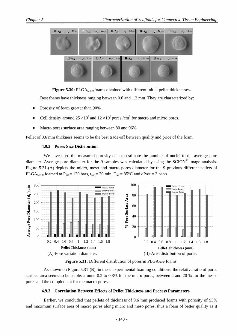
Chapter 5. Characterization of Scaffolds for Connective Tissue Engineering
- 143 -
Figure 5.30: PLGA50:50 foams obtained with different initial pellet thicknesses.
Best foams have thickness ranging between 0.6 and 1.2 mm. They are characterized by:
Porosity of foam greater than 90%.
Cell density around 25 ×103 and 12 ×106 pores /cm3 for macro and micro pores.
Macro pores surface area ranging between 80 and 96%.
Pellet of 0.6 mm thickness seems to be the best trade-off between quality and price of the foam.
4.9.2 Pores Size Distribution
We have used the measured porosity data to estimate the number of nuclei to the average pore diameter. Average pore diameter for the 9 samples was calculated by using the SCION® image analysis. Figure 5.31-(A) depicts the micro, meso and macro pores diameter for the 9 previous different pellets of
PLGA50:50 foamed at Psat = 120 bars, tsat = 20 min, Tsat = 35°C and dP/dt = 3 bar/s.
Pore Variation in Foam
Pellet Thickness (mm)
0.2 0.4 0.6 0.8 1 1.2 1.4 1.6 1.8
Ave
rage
Por
e D
iam
eter
( d
e ) m
0
50
100
150
200
250
300Micro PoresMeso PoresMacro Pores
Area Distribution of Pores
Pellet Thickness (mm)
0.2 0.4 0.6 0.8 1 1.2 1.4 1.6 1.8
% P
ore
Su
rfac
e A
rea
0
20
40
60
80
100 Micro PoresMeso PoresMacro Pores
(A)-Pore variation diameter. (B)-Area distribution of pores.
Figure 5.31: Different distribution of pores in PLGA50:50 foams.
As shown on Figure 5.31-(B), in these experimental foaming conditions, the relative ratio of pores surface area seems to be stable: around 0.2 to 0.3% for the micro-pores, between 4 and 20 % for the meso-
pores and the complement for the macro-pores.
4.9.3 Correlation Between Effects of Pellet Thickness and Process Parameters
Earlier, we concluded that pellets of thickness of 0.6 mm produced foams with porosity of 93% and maximum surface area of macro pores along micro and meso pores, thus a foam of better quality as it
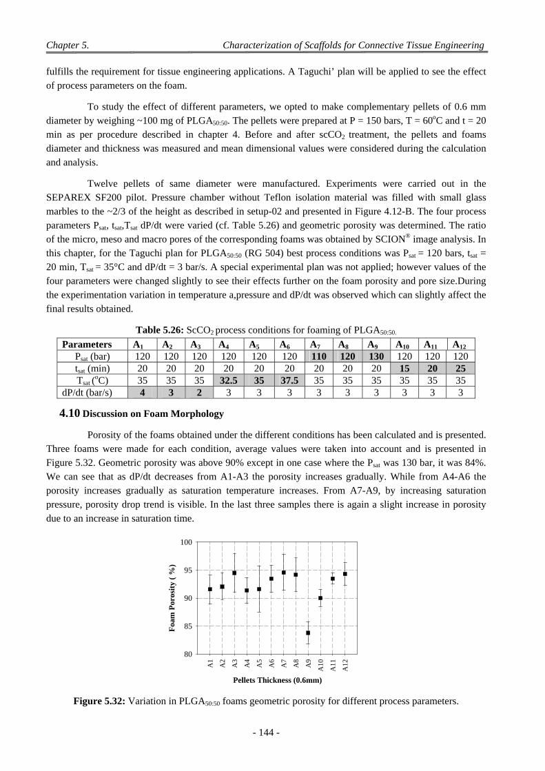
Chapter 5. Characterization of Scaffolds for Connective Tissue Engineering
- 144 -
fulfills the requirement for tissue engineering applications. A Taguchi’ plan will be applied to see the effect
of process parameters on the foam.
To study the effect of different parameters, we opted to make complementary pellets of 0.6 mm diameter by weighing ~100 mg of PLGA50:50. The pellets were prepared at P = 150 bars, T = 60oC and t = 20 min as per procedure described in chapter 4. Before and after scCO2 treatment, the pellets and foams diameter and thickness was measured and mean dimensional values were considered during the calculation
and analysis.
Twelve pellets of same diameter were manufactured. Experiments were carried out in the SEPAREX SF200 pilot. Pressure chamber without Teflon isolation material was filled with small glass marbles to the ~2/3 of the height as described in setup-02 and presented in Figure 4.12-B. The four process parameters Psat, tsat,Tsat dP/dt were varied (cf. Table 5.26) and geometric porosity was determined. The ratio of the micro, meso and macro pores of the corresponding foams was obtained by SCION® image analysis. In this chapter, for the Taguchi plan for PLGA50:50 (RG 504) best process conditions was Psat = 120 bars, tsat = 20 min, Tsat = 35°C and dP/dt = 3 bar/s. A special experimental plan was not applied; however values of the four parameters were changed slightly to see their effects further on the foam porosity and pore size.During the experimentation variation in temperature a,pressure and dP/dt was observed which can slightly affect the
final results obtained.
Table 5.26: ScCO2 process conditions for foaming of PLGA50:50.
Parameters A1 A2 A3 A4 A5 A6 A7 A8 A9 A10 A11 A12 Psat (bar) 120 120 120 120 120 120 110 120 130 120 120 120 tsat (min) 20 20 20 20 20 20 20 20 20 15 20 25 Tsat (
oC) 35 35 35 32.5 35 37.5 35 35 35 35 35 35 dP/dt (bar/s) 4 3 2 3 3 3 3 3 3 3 3 3
4.10 Discussion on Foam Morphology
Porosity of the foams obtained under the different conditions has been calculated and is presented. Three foams were made for each condition, average values were taken into account and is presented in Figure 5.32. Geometric porosity was above 90% except in one case where the Psat was 130 bar, it was 84%. We can see that as dP/dt decreases from A1-A3 the porosity increases gradually. While from A4-A6 the porosity increases gradually as saturation temperature increases. From A7-A9, by increasing saturation pressure, porosity drop trend is visible. In the last three samples there is again a slight increase in porosity
due to an increase in saturation time.
Foams Porosity Variation
Pellets Thickness (0.6mm)
A1
A2
A3
A4
A5
A6
A7
A8
A9
A10
A11
A12
Foa
m P
oros
ity
( %
)
80
85
90
95
100
Figure 5.32: Variation in PLGA50:50 foams geometric porosity for different process parameters.
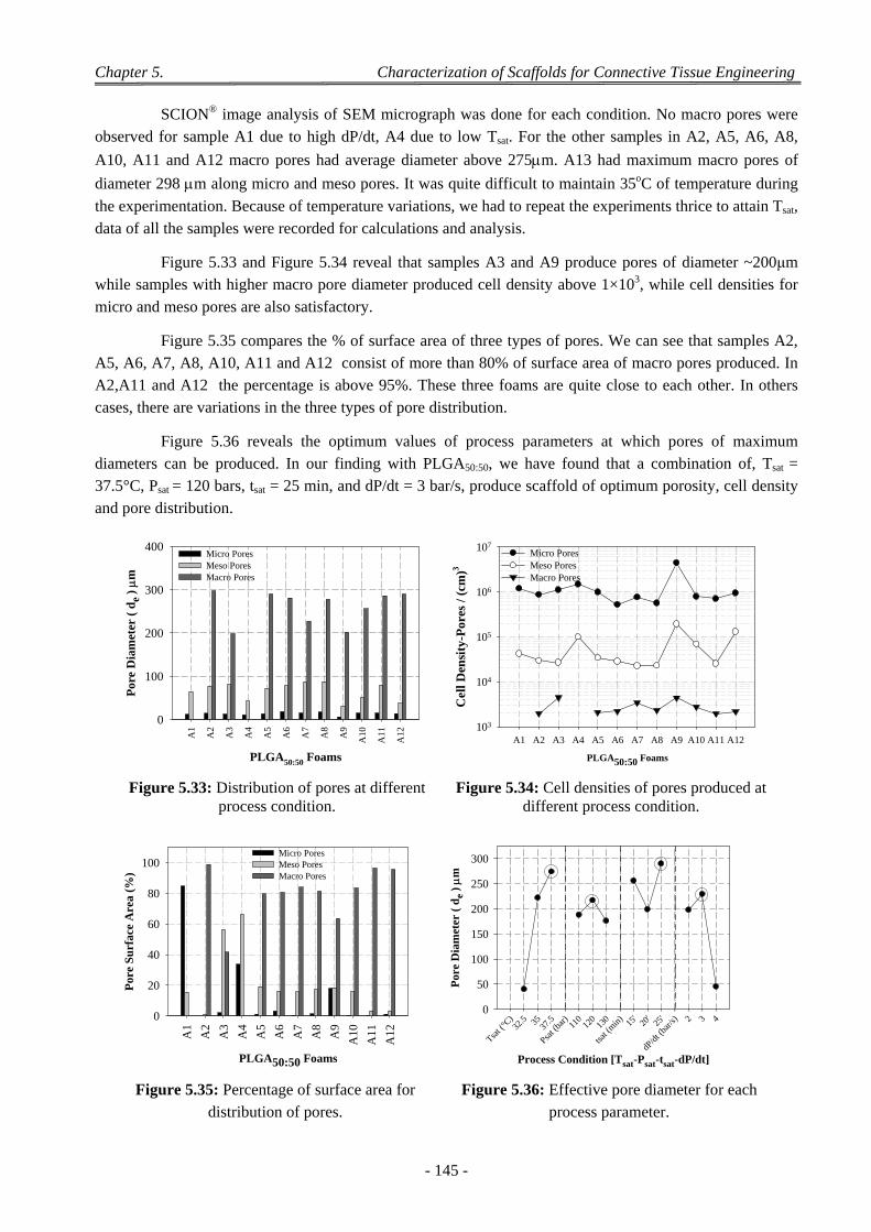
Chapter 5. Characterization of Scaffolds for Connective Tissue Engineering
- 145 -
SCION® image analysis of SEM micrograph was done for each condition. No macro pores were observed for sample A1 due to high dP/dt, A4 due to low Tsat. For the other samples in A2, A5, A6, A8,
A10, A11 and A12 macro pores had average diameter above 275m. A13 had maximum macro pores of
diameter 298 m along micro and meso pores. It was quite difficult to maintain 35oC of temperature during
the experimentation. Because of temperature variations, we had to repeat the experiments thrice to attain Tsat,
data of all the samples were recorded for calculations and analysis.
Figure 5.33 and Figure 5.34 reveal that samples A3 and A9 produce pores of diameter ~200μm while samples with higher macro pore diameter produced cell density above 1×10³, while cell densities for
micro and meso pores are also satisfactory.
Figure 5.35 compares the % of surface area of three types of pores. We can see that samples A2, A5, A6, A7, A8, A10, A11 and A12 consist of more than 80% of surface area of macro pores produced. In A2,A11 and A12 the percentage is above 95%. These three foams are quite close to each other. In others cases, there are variations in the three types of pore distribution.
Figure 5.36 reveals the optimum values of process parameters at which pores of maximum diameters can be produced. In our finding with PLGA50:50, we have found that a combination of, Tsat = 37.5°C, Psat = 120 bars, tsat = 25 min, and dP/dt = 3 bar/s, produce scaffold of optimum porosity, cell density
and pore distribution.
Pore Variation in Foam
PLGA50:50 Foams
A1
A2
A3
A4
A5
A6
A7
A8
A9
A10
A11
A12
Por
e D
iam
eter
( d
e ) m
0
100
200
300
400Micro PoresMeso PoresMacro Pores
Cell Density of Pores
PLGA50:50 Foams
A1 A2 A3 A4 A5 A6 A7 A8 A9 A10 A11 A12
Cel
l Den
sity
-Por
es /
(cm
)3
103
104
105
106
107Micro PoresMeso PoresMacro Pores
Figure 5.33: Distribution of pores at different process condition.
Figure 5.34: Cell densities of pores produced at different process condition.
Area Distribution of Pores
PLGA50:50 Foams
A1
A2
A3
A4
A5
A6
A7
A8
A9
A10
A11
A12
Por
e S
urf
ace
Are
a (%
)
0
20
40
60
80
100Micro PoresMeso PoresMacro Pores
PLGA50:50 Optimum Parameters
Process Condition [Tsat-Psat-tsat-dP/dt]
Tsat (
°C)
32.5 35 37
.5
Psat (
bar)
110
120
130
tsat (
min)
15'
20'
25'
dP/dt
(bar/
s) 2 3 4
Por
e D
iam
eter
( d
e ) m
0
50
100
150
200
250
300
Figure 5.35: Percentage of surface area for distribution of pores.
Figure 5.36: Effective pore diameter for each process parameter.
Chapter 5. Characterization of Scaffolds for Connective Tissue Engineering
- 146 -
One can see the effects of all the process parameters on the pore size. Increasing Tsat ultimately improves the pore diameter, and pore diameter is decreased by increment of Psat and dP/dt. There was a slight increase in the pore diameter of foam by increment of tsat. So the process parameters have been improvised by performing these experiments. A foam was then produced at this optimized condition and
from analysis, the porosity obtained was 93% and diameters for micro, meso and macro pore was 14m,
97m and 276 m respectively.
5 Conclusion
Different types of polylactides including polylactic acid and poly(lactic co-glycolic acid) have been characterized in details. The composition of each polymer was also discussed as it has a pivotal role on the properties of the final porous scaffolds produced. Foams were made with pure polylactic acid and with blends of polylactic acid and polylactic co-glycolic acid in order to analyze the effect of LA/GA composition during the foaming process and porosity of the foam. Different experimental designs were used to attain optimized porosity and pore size distribution.
Firstly, we must admit that the consideration of the results of the 24, Taguchi and initial Doehlert plan is difficult. During these experiments, we have not noticed the important effect of the volume constraint and the position of the pellet. Indeed, these two parameters affect the pore size. We have encountered important heterogeneities within the cross-sections micrographs and very different pore sizes for the scaffolds which were processed in the same chamber. For this reason, we have decided to change the experimental setup. We have removed the Teflon isolation to gain volume and we have filled the chamber with small glass balls. After that, only one pellet has been placed on the holed grill which has been positioned above the glass balls. For the following experiments, we have found that the pore size increases with decreasing saturation pressure and depressurization rate. Best results have been achieved within the
range of 128 and 138μm for Psat = 100 bar, Tsat = 36.5°C, tsat = 60 min. and dP/dt = 1.25 bar /s.
Finally, detailed emphasis was laid down on the effect of process parameters such as saturation pressure, saturation temperature and saturation time and depressurization rate during foaming process.
Optimum thickness of the pellet was finalized for the experimentation process.
Lirela seconde partie
de la thèse