CRED WORKING PAPER N o 2020-8

Does Labor Income React more to Income Tax or Means-TestedBenefit Reforms?

April 2020

Michaël Sicsic∗

∗INSEE, and CRED(TEPP), Université Paris 2 Panthéon-Assas. E-mail: sicsic.michael@gmail.com. Address:Insee, 88 avenue Verdier, CS 70058, 92541 Montrouge, France. I am grateful to Etienne Lehmann and LaurenceRioux for their guidance and advice throughout this project. I thank Antoine Bozio, Clément Carbonnier, AntoineFerey, Malka Guillot, Marie Obidzinski, Corinne Prost, and Maxime Tô for their helpful comments and suggestionson previous versions of this paper (which circulates with the title "The Elasticity of labor Income: Evidence fromFrench Tax and Benefit Reforms, 2006-2015"), as well as participants of the 67th ASFE annual meeting, 16th journéesLAGV, 35e JMA congress, 17th International Conference of APET, and seminars and workshops at PSE, CREDParis 2, and INSEE.

1

Does Labor Income React more to Income Tax or Means-

Tested Benefit Reforms?

Michaël SICSIC

Abstract. I provide estimates of the compensated elasticity of labor income with respect to the

Marginal Net-of-Tax Rate on the 2006-2015 period for France. I exploit not only income tax

reforms but also means-tested benefits reforms. I use semiparametric graphical evidence and

a classic 2SLS estimation applied to a rich data set including both financial and socio-

demographic variables. I obtain an estimated compensated elasticity around 0.2-0.3 in

response to income tax reforms, around 0.1 in response to in-work benefit reforms, while I

found no statistically significant response to family allowance reforms. I show that the

difference between elasticities contradicts the prediction of the classical labor supply model.

One possible explanation is that income tax reforms are more salient and better perceived than

benefit reforms. This suggests that benefit reforms may be more efficient in reducing

inequalities than income tax reforms due to their lesser behavioral responses. Another

contribution is to highlight heterogeneous elasticities depending on income, age, family

configuration and education. Results are very robust to a large number of robustness checks,

unlike previous studies on the US economy.

Keywords: elasticity of labor income; income tax; means-tested benefit; marginal tax rate.

JEL classification: H21; H24; H31; J22; C26.

____________________________________________

Introduction

Income tax and means-tested benefits are the main policy instruments to increase redistribution

and reduce inequality. While income tax is often put forward, benefits also play an important

role: they account for about three quarters of the reduction of inequality from market income to

disposable income in OECD countries1 according to Causa and Hermansen (2017). As any

redistributive instruments, these tools tend to reduce labor supply and thereby incomes.

Whether these detrimental effects of redistribution are more important for income tax reforms

or means-tested benefit reforms is an open question that the present paper addresses empirically.

In this article, I estimate the response of labor income to income tax reforms and reforms of

means-tested benefits implemented in France between 2006 and 2015 using the framework of

the elasticity of taxable income (ETI) literature (Saez et al., 2012). This framework makes it

possible to estimate the compensated elasticity with respect to marginal net-of-tax rates, MNTR

(see Gruber and Saez, 2002), which is the relevant statistic for welfare analysis. While the

theoretical framework underlying the ETI method is generally applied to income tax in the

literature, I generalize it with n different types of tax schedules, including means-tested benefits.

I highlight what are the theoretical predictions for comparison between elasticities. With this

framework, I estimate the compensated elasticities of labor income with respect to MNTR and

the average net-of-tax rates, for three different types of transfers: income tax, in-work benefits

and family benefits. In addition to the econometric estimation, I also implement non-parametric

regressions (with the methodology of Weber, 2014) of the relationship between MNTR and

labor income, which enables me to obtain a graphical visualization of the effect. Since I do not

only want to exhibit elasticity from income tax but also from means-tested benefits, which

depend on a different income base than taxable income, I focus on individual labor income

responses, the only margin of response comparable between all transfers. Since labor income

does not include tax deductions (unlike taxable income2) and is less subject to retiming

phenomenon than other income such as capitalized earnings, I am thus interested in the “real”

response to taxation.

I use reforms implemented in France between 2006 and 2015. Working with French data

enables me to compare responses to income tax and means-tested benefits because: (i) means-

tested benefits have a significant weight (more than 3% of GDP, i.e., close to the weight of the

income tax in France), and (ii) taxes and benefits were substantially reformed over the period

2006-2015 covered in this study. Indeed, the income tax schedule was reformed several times

(number of brackets, marginal tax rates, bracket levels, and other mechanisms such as the

1 The exact number depends on whether pensions, unemployment benefit and social security contributions (SSC) are taken

into account in the redistribution. The OECD statistics are on working age population, thus they do not take into account

pensions. See also Guillaud et al. (2019) for a discussion on this issue. According to the distributional national accounts of

Piketty et al. (2018), “Transfers play a key role for the bottom 50%” (in reducing inequality). 2 Tax deductions are a factor that can lead to a higher elasticity in the short term. These deductions are not always negative

for the economy as a whole, since they may increase tax revenues at other times or for different tax bases, or lead to positive

externalities (e.g., for itemized deductions for charitable giving). Thus, Chetty (2009) shows that the ETI is no longer a

sufficient statistic and Doerrenberg et al. (2014) have proved this empirically.

quotient familial), an in-work benefit scheme was created in 2009 (RSA activité), and family

benefits have been substantially reformed since 2012. This number of reforms is also important

for identification and econometric issues. Firstly, there were up and down changes in marginal

tax rates (MTR) depending on the year, and changes in bracket cutoffs that moved groups of

taxpayers into different brackets. More precisely, the 2006-2015 period can be divided in two

separate subperiods influenced by opposite political contexts. In 2007, President Sarkozy

launched several conservative reforms aiming to “make work pay”, and mostly to reduce MTR.

After his election in 2012, the left-wing President Hollande launched several reforms aiming to

reduce income inequality and restore public finances (a large increase in means-tested benefits

for poor people, a large decrease in the ceiling of some family allowances, and a tax increase

for wealthy families) and thus, to increase MTR. This variability of MTR enhances our ability

to identify responses to tax reform by mitigating the effect of natural (non-tax) trends in income

inequality, an important source of concern in US studies (Saez et al., 2012; Weber, 2014).

Secondly, different reforms such as changes to the ceiling of the tax advantage for children

(quotient familial) led to different variations in marginal tax rates for the same level of income

depending on family composition and the number of children. This is a very rich source of

identification3 and it alleviates the problem caused by the fact that mean reversion controls and

tax change instruments depend on the same variable - the base year income - which can blur

identification. Thirdly, the income distribution is stable over the period 2006-2015 in France,

thus avoiding problems of heterogeneous income trends. I test different econometric

specifications, in particular different base-year income controls (to account for trend

heterogeneity and mean reversion), different instruments and a large number of controls. The

data used are from the French Enquête Revenus Fiscaux et Sociaux (ERFS), a match between

fiscal records, social administrative data, and the labor force survey, covering a total of more

than 100,000 people each year. MTR are simulated using the INES microsimulation model

developed by INSEE and DREES. The ERFS data allow me to simulate means-tested benefits

and to have better control over econometric estimation through a wide variety of labor market,

education, profession, and socio-demographic information.

I obtain an estimated compensated elasticity around 0.2-0.3 in response to income tax reforms,

around 0.1 in response to in-work benefit reforms, while I found no statistically significant

response to family allowance reforms. These results are very robust to a large number of

robustness checks. I show that the difference between elasticities contradicts the prediction of

the classical labor supply model. One possible explanation for the stronger reactions to income

tax reforms compared to benefit reforms is that income tax reforms are more salient and better

perceived than benefit reforms. This is therefore linked to the literature on tax salience and tax

inattention (Chetty et al., 2009; Rees-Jones and Taubinsky, 2016; Chetty et al., 2013; Feldman

et al., 2016; De Bartolone, 1995; Ito, 2014). Recently, Bosch et al. (2019) explain the non-

3 This type of reform has already been used by Piketty (1999) and Cabannes et al. (2014) to estimate ETI. It may be a

response to Saez et al.’s (2012, p. 43) call for better sources of identification: "researchers should look for better sources of

identification, for example, alternative income tax systems that affect taxpayers differently."

bunching response to kinks and notches in the Dutch system of cash transfers in terms of lack

of salience and inattention. A consequence of the higher behavioral response of income tax to

benefits is that benefit reforms could be more effective in reducing inequalities (or reducing the

government deficit) than income tax, a finding that echoes Doerrenberg and Peichl (2014).4

By estimating the elasticity of different transfers, I can also estimate an overall labor income

elasticity with respect to all transfers around 0.1. This overall elasticity is the relevant statistic

for optimal tax exercises. Since optimal marginal tax rates refers to the effective tax rate of all

the transfers depending on income, this elasticity that takes into account the overall tax and

benefit system should be used in optimal tax formulas (instead of using only income tax

reforms, as usually done).

Thanks to the variety of reforms I use for the identification (which affect the whole income

distribution), I can estimate different elasticities for different types of people (level of income,

family composition, education, etc.) for income tax and all transfers. I find that the elasticities

are higher for the top decile (about twice that of the entire sample), for the self-employed, for

single people without children, for people between the ages of 20 and 30 and above 50, as well

as people with higher qualifications. The importance of taking into account heterogeneous

elasticities among workers earning the same income has been highlighted by Kumar and Liang

(2017) and Jacquet and Lehmann (2020).5

This paper is related to the literature estimating the response to tax and benefit reforms. Firstly,

it is linked to the ETI literature which estimates elasticities to fiscal reforms (Auten and Caroll,

1999; Gruber and Saez, 2002; Kopczuk, 2005; Saez et al., 2012; Weber, 2014)6 and especially

elasticities applied to labor income (Blomquist and Selin, 2010; Kleven and Schulz, 2014;

Lehmann et al., 2013). The paper is also related to the literature using quasi-experimental

frameworks to evaluate the response to benefit reforms, and to the structural approach which

estimates elasticity of labor supply with respect to net-of-tax wage rate, based on a model for

optimizing behavior.7 Lastly, it is also related to papers estimating the behavioral response to

French tax reforms (Piketty, 1999; Carbonnier, 2014; Lardeux, 2018; Guillot 2019; Pacifico,

2019; Bach et al., 2019; Aghion et al., 2019; Lefebvre et al., 2019). The present paper makes

four contributions to these strands of literature. (i) The main contribution is to jointly estimate

4 The work by Doerrenberg and Peichl (2014) suggests that behavioral responses are lower for benefits, but without explicitly

estimating the respective responses. They acknowledge challenges in identifying the causal effect, and thus highlight the fact

that “Considering the political importance and widely held debates about (increasing) inequality around the world, the

research question imposed in our paper needs further attention”. I try to address this research question in this paper. 5 It has also been highlighted by Gruber and Saez (2002): they show that Feldstein’s grouping method is consistent only if the

two groups (treated and control) have identical elasticities, which is not the case. Jacquet and Lehmann (2020) emphasize that

multidimensional heterogeneity substantially affects optimal marginal tax rates through a composition effect (top optimal

marginal tax rates with a composition effect are for instance up to 20.3 percentage points compared to the top tax rate when

heterogeneity is one-dimensional) and that “Our results put the stress on the need for empirical studies on sufficient statistics

for different demographic groups”. 6 See also Giertz (2007), Cabannes et al. (2014), Doerrenberg et al. (2014), Gelber (2014), Matikka (2015), Kumar and Liang

(2017), Hermle and Peich (2018), Neisser (2018), Jongen and Stoel (2019), Creedy and Gemmell (2019). See also papers that

compare the ETI method with bunching (Aronsson et al., 2017) or discrete choice model (Thoresen and Vatto, 2015). 7 Pioneered by Hausman (1985); see reviews by Blundell and MaCurdy (1999), Keane (2011) and Evers et al. (2008).

Discrete choice models have gained popularity since van Soest (1995): see Bargain and Peichl (2013) for a literature review.

responses to income tax and means-tested benefit reforms in a unique framework and with the

same data, and to be able to compare elasticities. I also develop a framework to highlight the

theoretical prediction. The compensated elasticity I obtain of 0.2-0.3 for tax reforms is fully

consistent with the recent ETI literature. The low response to benefit reforms is in line with

some French papers8 and recent results of Bosch et al. (2019) in the Netherlands, who find non-

bunching responses to kinks and notches in the Dutch system of cash transfers. But these results

of the literature cannot be compared with each other because they do not use the same

methodology and data. (ii) I am also able to estimate an elasticity with respect to the effective

MNTR, taking into account the overall tax and benefit system. (iii) I estimate heterogeneous

elasticities, whereas previous research on ETI mainly estimates elasticities for high incomes9

(because they mainly exploit income tax changes at the top of the income distribution10).

Results depending on level of income and type of income are in line with Gruber and Saez

(2002) and Kleven and Schulz (2014), and other results depending on family configuration,

age, or education are new compared to the ones already present in the ETI literature. (iv) I find

very robust estimates (especially compared with the previous studies on the US) for a wide

variety of robustness checks, thanks to the reforms used, the data11 and the context (see above).

The rest of the paper is structured as follows. Section 1 presents the theoretical framework and

empirical strategy. Section 2 describes the reforms used for identification. Section 3 describes

the data used and presents some descriptive statistics. Section 4 presents the empirical results

and the last section concludes.

1. Conceptual framework

1.1. Theoretical model

1.1.1. Model

The objective of this theoretical section is to explain the relationship between labor income and

the marginal tax rate (MTR). I follow the usual framework on ETI based on the classical labor

supply model (Saez et al., 2012; Lehmann et al., 201312). While this framework is generally

applied to income tax in the literature, I generalize it with n different types of tax schedules,

especially monetary means-tested benefits. Social security contributions (SSC) are not taken

into account in these n tax schedules because gross incomes (on which SSC depend) are not

8 The low response to RSA reform is in line with Briard and Sautory (2012) and Bargain and Vicard (2014) in France. 9 Apart from the work of Gruber and Saez (2002), Cabannes et al. (2014), Kleven and Schulz (2014) and Jongen and Stoel

(2019) who estimate different elasticities depending on income distribution. 10 And especially, the Tax Reform Act of 1986 (TRA86) in the US for identification. In France, Piketty (1999) focuses on top

income while Lehmann et al. (2013) focuses on poor workers. 11 This is due to (i) the richness of the database (socio-demographics variable), and (ii) the fact that the ERFS database

contain only few very high incomes, which has the advantage of lessening some problems particular to this population in the

ETI estimation (heterogeneous income trends, means reversion, income-shifting between capital/labor). 12 Lehmann et al. (2013) identify income effects in a more consistent way with the theoretical framework.

available in the data, and because during the period under review, there was no good reform to

identify the elasticity of SSC.13

Individuals choose (c, z) where c is disposable income and z is posted labor income.14

Individuals maximize a utility function U(c , z) which increases with c and decreases with z

because earning a higher labor income z requires the worker to work harder. The tax-benefit

system consists of n transfers dependent on posted labor income (i.e., labor income net of

payroll tax but gross of income tax): income tax, in-work benefit, family and housing benefits,

social minimum income supports, etc. yj is the labor income minus the jth transfer Tj(z). So we

have yj = z − Tj(z). The marginal net of tax rate (MNTR) of transfer j is τj and the average-

net-of tax rate (ANTR) of the transfer j is ρj with j= 1 to n. It is a static model where there are

no savings and consumption is equal to disposable income.

On the linear part of each tax bracket, denoting the virtual income Rj we have for j=1 to n:

yj = zτj + Rj and 𝜌𝑗 =𝑦𝑗

𝑧= 𝜏𝑗 +

𝑅𝑗−1

𝑧

Thus, the amount of tax for each transfer is for j from 1 to n: Tj(z) = z − yj = (1 − τj)z−Rj

The disposable income (or consumption 𝑐) is therefore:

𝑐 = 𝑧 − ∑ 𝑇𝑗(𝑧) =𝑛

𝑗=1𝑧 − ∑ {(1 − 𝜏𝑗)𝑧 − 𝑅𝑗} = 𝑧 {1 − 𝑛 + ∑ 𝜏𝑗

𝑛

𝑗=1

} +𝑛

𝑗=1∑ 𝑅𝑗

𝑛

𝑗=1

(1)

Labor income is determined by the Marshallian behavioral function:

𝑧 = 𝑍(𝜏1, 𝜏2 , … , 𝜏𝑛, 𝑅1, 𝑅2 , … , 𝑅𝑛)

Differentiating this function leads to:

∆𝑧

𝑧= ∑ (

∆𝜏𝑗

𝜏𝑗(

𝜏𝑗

𝑧

𝜕𝑍

𝜕𝜏𝑗) + (

∆𝑅𝑗

𝑧

𝜕𝑍

𝜕𝑅𝑗))

𝑛

𝑗=1

(2)

with (τj

z

∂Z

∂τj) the uncompensated elasticity with respect to the jth MNTR τj

We are interested in compensated elasticity with respect to the MNTR, which is the relevant

parameter for welfare and optimal tax analyses. A compensated tax reform is defined as a

simultaneous change of the MNTR (∆τj) and virtual income (∆Rj), so that the amount of tax

paid on initial labor income z remains unchanged. Thus, if the reform is compensated for j=k

then ∆Rk = −∆τjz, and if j ≠ k then ∆τj = ∆Rk = 0. Then, by defining βτk the compensated

elasticity with respect to the MNTR of the transfer k, we find the Slutsky equation:15

13 It should also be noted that, to take into account social security contributions, the conceptual framework must be modified

to take into account the different tax bases, as Lehmann et al. (2013) do. 14 The labor income I am interested in can be written z=wl where w is the hourly wage. Blomquist and Selin (2010) show that

w is not exogenous (as in the classical literature on labor supply), but can depend on effort and tax rates.

15 The previous calculation leads, by replacing in (2) and rearranging to have: ∆𝑧

𝑧=

∆𝜏𝑘

𝜏𝑘 (𝜏𝑘

𝑧

𝜕𝑍

𝜕𝜏𝑘− 𝜏𝑘 𝜕𝑍

𝜕𝑅𝑘). Then, we find the

Slutsky equation inside the brackets of this equation.

𝛽𝜏𝑘 =

𝜏𝑘

𝑧(

𝜕𝑍

𝜕𝜏𝑘) − 𝜏𝑘

𝜕𝑍

𝜕𝑅𝑘 (3)

By rearranging equation (3)16 and putting in (2), we obtain:

∆𝑧

𝑧= ∑ (𝛽𝜏

𝑘∆𝜏𝑘

𝜏𝑘+

𝜕𝑍

𝜕𝑅𝑘(∆𝜏𝑘 +

∆𝑅𝑘

𝑧))

𝑛

𝑘=1

(4)

Then, by using ρk =yk

z= τk +

Rk

z we have: ∆ρk = ∆τk +

∆Rk

z−

Rk

z

∆z

z

However, labor income must be maintained at its initial value z∗ to have a compensated reform

(Lehmann et al., 2013). Thus I define the change of the average-net-of tax rate of the transfer k

while keeping the labor income fixed at its initial value ∆ρ̅k, in the following way:

∆�̅�𝑘 = ∆𝜏𝑘 +∆𝑅𝑘

𝑧∗ (5)

So by putting equation (5) in (4), we obtain (6):

∆𝑧

𝑧= ∑ (𝛽𝜏

𝑘∆𝜏𝑘

𝜏𝑘+

𝜕𝑍

𝜕𝑅𝑘∆�̅�𝑘)

𝑛

𝑘=1

(6)

This gives the following final equation, defining the compensated elasticity with respect to the

ANTR of the transfer k by: βρk = ρk ∂Z

∂Rk

∆𝑧

𝑧= ∑ (𝛽𝜏

𝑘∆𝜏𝑘

𝜏𝑘+ 𝛽𝜌

𝑘∆�̅�𝑘

𝜌𝑘)

𝑛

𝑘=1

(7)

1.1.2. Predictions of reference model

In the labor supply reference model, z is determined by maximizing U(c , z) under budgetary

constraint c = zτ + R , and therefore:

𝑧 = 𝑎𝑟𝑔𝑚𝑎𝑥𝑧 𝑈(𝑧𝜏 + 𝑅 , 𝑧) = Ω (𝜏, 𝑅)

The solution of the program Ω depends only on the global marginal net-of-tax rate τ and the

global virtual income R. By matching the budgetary constraint of this model to equation (1),

we obtain:

τ = 1 − n + ∑ τjnj=1 and R = ∑ Rjn

j=1

In the model explained above, labor income z was determined by the behavioral function

z = Z(τ1, τ2 … τn, R1, R2 … , Rn). Thus we have: Ω (τ, R) = Z(τ1, τ2 … τn, R1, R2 … , Rn)

Differentiating the two sides of the equation gives:

∂Z

∂τk =∂ Ω

∂τ and

∂Z

∂Rk =∂ Ω

∂R for k between 1 and n

Using (3) we have: βτk =

τk

z

∂Z

∂τk − τk ∂Z

∂Rk = τk (1

z

∂ Ω

∂τ−

∂ Ω

∂R ) which leads to equation (8):

16 By rearranging equation (3), we have: 𝜏𝑘

𝑧(

𝜕𝑍

𝜕𝜏𝑘) = 𝛽𝜏𝑘 + 𝜏𝑘 𝜕𝑍

𝜕𝑅𝑘 , which lead to 𝜏𝑘

𝑧(

𝜕𝑍

𝜕𝜏𝑘

∆𝜏𝑘

𝜏𝑘 ) = 𝛽𝜏𝑘 ∆𝜏𝑘

𝜏𝑘 +𝜕𝑍

𝜕𝑅𝑘 ∆𝜏𝑘

βτ1

τ1=

βτ2

τ2= ⋯ =

βτn

τn (8)

In the result section we test this prediction by empirically estimating each elasticity.

1.2. Empirical strategy

I estimate the empirical counterpart of (7) for an individual i employed at date t-1 and t:

∆log zi,t = α + ∑ (𝛽𝜏𝑘 ∆𝑙𝑜𝑔 𝜏𝑖,𝑡

𝑘 + 𝛽𝜌𝑘 ∆�̅�𝑖,𝑡

𝑘 )

𝑛

𝑘=1

+ γ Xi,t−1 + δ It + φ log zi,t−1

+ ∑ ϑ splines(zi,t−1) + μi,t

10

1

(9)

Where:

- Δ is the time difference between dates t and t-1,

- zi,t is the posted labor income of individual i in period t,

- βτk is our interest parameter, the compensated elasticity with respect to the MNTR of the

transfer k: it is equal to the percentage change in labor income associated with a 1% increase

in the MNTR.

- βρk is the elasticity with respect to ρ̅k (the ANTR of the transfer k while keeping the labor

income fixed at its initial value, see eq. 6).

- Xi,t−1 a vector of individual and firm characteristics (labor market, education, characteristics

of the firms, socio-demographic variables, etc.) observed in the base period (i.e. t-1),

- It time indicators

- μi,t an error term that reflects unobserved and time-varying heterogeneity.

Equation (9) is estimated using the two-stage least squares (2SLS) method, which provides

local average treatment effect (LATE) estimators as shown by Angrist, Imbens, and Rubin

(1996). Using a first difference model allows to control for unobserved time-invariant

heterogeneity such as individuals’ and firms’ characteristics, or different preferences for work

and leisure. One-year time variations are used because of data that can only be matched for two

consecutive years (see data section): I therefore estimate a short-term response. Some articles

have used a three-year period (Gruber and Saez, 2002; Kleven and Schulz, 2014) to estimate

medium-term responses, but Weber (2014) highlights that these 3-year differences capture a

combination of short, medium and long-term responses, making interpretation difficult. In

addition, the estimates are not affected by these choices of temporary difference, according to

Weber's (2014) estimates. This specification assumes that there are no local accumulation

points at the discontinuities of MTR to avoid creating bias in the estimate (Kleven and Schulz,

2014): since no bunching is found on labor income in France,17 this should not be a problem

17 Lardeux (2018) only finds bunching for taxpayers who can manipulate a certain tax deduction, at a certain threshold.

for the estimate. Note also that I focus on individual18 labor income response, the only margin

of response comparable between all transfers.19 I am thus interested in the “real” response to

taxation, closer to a sufficient statistic for welfare analysis (Chetty, 2009).

According to equation (7), ρ̅i,tk is the variation in the average-net-of tax rate of the transfer k

computed while keeping the real labor income fixed at its pre-reform value. Then, ∆log ρ̅i,tk =

log ρ̅i,tk − log𝜌i,t−1

k and ρ̅i,tk = 1 −

Ttk(z̅i,t−1)

z̅i,t−1 with k=1 to n; and z̅i,t−1 = 𝑧i,t−1 𝜋𝑡−1 where 𝜋𝑡−1

denotes inflation between years t-1 and t.

The most apparent methodological challenge in estimating equation (9) concerns the

endogeneity of MNTR, which creates a correlation between ∆logτi,tk , ∆logzi,t and the error term.

To address the endogeneity of MNTR τi,tk , we need an instrument. By far the most widely used

instrument (first introduced by Auten and Carroll, 1999, and popularized by Gruber and Saez,

2002) is the value of τi,tk if the individual income was z̅i,t−1 (income in year t-1 adjusted for

inflation between t-1 and t) and if the tax code was that of year t. This instrument is therefore

exogenous to post-reform incomes.

The instrument (which I will call the "Auten and Carroll type" or A&C type) for ∆logτi,tk is

therefore:

∆logτi,tk

= logτi,tk

− logτi,t−1k with τi,t

k= 1 −

∂Ttk(z̅i,t−1)

∂z̅i,t−1 . This instrument is sometimes referred

to as the predicted, mechanical, or synthetic net-of-tax rate. Hence the instrument is equal to

the log change in the MNTR if (real) labor income was kept unchanged. This instrument

therefore captures how a taxpayer is exposed to tax reforms given her base-year income.

However, this instrument depends on pre-reform income (in t-1) and can therefore be correlated

with the error term if the pre-reform income is correlated with the error term. This may occur

through two channels discussed in the ETI literature: (i) when there are non-tax changes in labor

income that may affect groups differently (“heterogeneous income trends”); or (ii) due to a

“return to the mean” phenomenon (“means reversion”) (see Saez et al., 2012). Firstly,

heterogeneous income trends pose a problem if there are non-tax related changes in gross labor

income between income groups, due for instance to skill-biased technical progress resulting

from globalization. The risk when evaluating a tax reform is to attribute changes in gross labor

income to the tax reforms rather than to these non-tax causes, thereby causing a bias in the

estimation.20 Secondly, permanent and transitory income components are included in pre-

18 Note that there is an income-splitting mechanism in the French income tax system (which is not however completely dual

since the earned income tax credit style schedule is individual). Creedy and Gemmell (2019) show that in the presence of

individual income taxation, ETI could be expected to be different when those estimates are obtained while treating the

behavior of couples in households as if they were separate individuals. Here this criticism does not apply since there is no

individual income taxation in France. 19 One example is that the household unit used for benefit is not the same as the tax unit used for income tax. Moreover,

deductions and credits are taken into account for income tax but not for benefits. 20 For instance, when evaluating a reform like TRA86 in the US that reduced marginal tax rates more for top incomes, the

trend of widening income inequality may lead one to attribute the fact that income increased more in the treatment group than

in the control group to TRA86 instead of to trends (Saez and Gruber, 2002).

reform income, which creates a means-reversion problem. For instance, an individual with an

unusually low (respectively high) labor income in period t−1 is very likely to have a higher

(lower) one at t, if she finds (loses) a job for instance. These non-tax causes can blur the

identification if they are not controlled for.

The ETI literature addresses these two sources of problems by adding initial income as a control

variable: log-linearly for Auten and Carroll (1999) and with a richer functional form in splines21

for Gruber and Saez (2002). One of the difficulties is that these controls and instruments depend

on the same variable (base year income), which can "destroy identification" (Gruber and Saez,

2002) if there are only two years of data. These risks are much lower in this study for the

following reasons: (i) the number of years of data (9 years, see section 3); (ii) the up and down

changes in MTR that occurred between 2006 and 2015, which are nonlinear functions of pre-

reform (see section 2), (iii) the asymmetry of MTR changes for the same income level (see

section 2), (iv) the use of periods with and without tax changes (Thoresen and Vatto, 2015).

Given the above and the fact that the distribution of income is relatively stable in France (see

Figure A4 in appendix B), we expect that the tax changes used will not systematically be

correlated with the pre-reform income level and therefore that the issue of controlling the effects

of income before the reform should be less severe than in the US studies. In the robustness

checks, I test various methods of pre-reform controls and especially specification proposed by

Kopczuk (2005), which takes into account splines of the log deviation of base-year income to

income in the preceding year (to account for mean reversion and other transitory income effects)

and splines of the labor income in the year preceding the base year (to control for heterogeneous

changes in the income distribution).22

Robustness checks are also carried out on the instruments. I test the instrument proposed by

Weber (2014)23 which is also based on the same idea of "predicted" evolution of the MNTR but

by replacing the initial income by a lag income. The instrument thus corresponds to the value

of τi,tk after tax reform if individuals' incomes were those of previous years (years t-2, t-3,...).

Weber (2014) highlights the fact that the instruments are exogenous with two delays

(using log zi,t−2). Since the data used contain labor income for years t-1 and t-2 for employees

(but not for self-employed workers), I can test a "Weber type" instrument on this population,

which is the value of τi,tk if the income of the individual i was z̅i,t−2 (adjusted for inflation) and

the tax legislation was that of year t.

Thus, the Weber type instrument for the ∆τi,tk is:

∆log τ̿i,tk = log τ̿i,t

k − log τi,t−1

k with τ̿i,t

k = 1 −∂Tt

k(z̅i,t−2)

∂z̅i,t−2 and τi,t−1

k= 1 −

∂Tt−1k (z̅i,t−2)

∂z̅i,t−2

21 Splines are linear functions in pieces with five, ten or more components. 22 Since the income for year t-2 is not known for the entire population (only for employees), we adopt the Gruber and Saez

specification in our basic specification and test the robustness controls in Kopczuk (2005) for employees only. 23 This instrument was also used by Lehmann et al. (2013).

2. Legislation and reforms used

In this section, I describe the main tax and benefit reforms that I use as a source of identification

and which were implemented during the 2006–2015 period covered by this study.24 Appendix

A gives further details on all the reforms used and gives an overview of the French legislation

on income tax and benefit.

2.1. Income tax reforms

Over the 2006–2015 period, there were several changes in the income tax code, which are

illustrated in the following graphs.

Firstly, the MTR was modified several times for high income earners (see Figure 1, which

summarizes the changes of the top and bottom marginal effective tax rates, METR25):

- the MTR was reduced in 2017 from 48.1% to 40% for the top incomes (see Table A1,

Appendix A) and the number of brackets changed.

- In 2012, two additional brackets (adding 3% and 4% to the top MTR) were created for

individuals with income above 250,000 euros (twice this amount for couples) and

500,000 euros (“contribution exceptionnelle sur les hauts revenus”), leading to a top

MTR of 45%.

- In 2013, an additional 45% bracket was created for income above 150,000 euros. It led

to a 49% higher MTR, taking into account the 2012 reform.

Secondly, the METR increased for low income brackets because of the change in the décote

parameter26 in 2014 (from 8% to 21% in 2014 and then 27% in 2015, see Figures 1 and 2).

Moreover, in 2014, an exceptional tax reduction took place at the bottom of the distribution,

increasing the METR to 121% in the differential zone for single people and 114 % for couples

(Sicsic, 2018). This tax reduction was cancelled in 2015, leading to a sharp fall in MTR in a

range of incomes (between 2.2 and 2.3 times the minimum wage for a couple, Figure 2).

Thirdly, the ceiling of the tax advantage for children decreased in 2013 and 2014 (from 2,336

euros per child to 2,000 euros in 2013 and then 1,500 euros in 2014). This reform led to different

variations in the MTR for the same level of income according to family composition and is

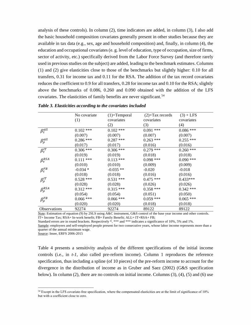
therefore an important source of identification.27 Figure 3 shows for instance that the 2014

reform increased MTR by 16% for a single person with one child earning between 2.8 and 3.4

24 Other reforms are detailed in Appendix A. Note that housing allowances are not taken into account because they were not

reformed over the period, and reforms on capital income and social security contributions are not taken into account because

they do not affect marginal tax rates (MTR) on net labor income. It should also be noted that the income taken into account is

different for each transfer: I do not enter this level of detail thereafter for the sake of simplification, but these differences are

fully taken into account in the simulation of each transfer (see section 3.3). 25 The METR include several features of the income tax code such as the 20% rebate before 2007, the décote and the

exceptional contribution on high incomes. 26 The décote is a tax deduction for income which raises the point of entry into income tax as well as the marginal tax rate just

above, and thus changes the marginal tax rate for the bottom of the scale (see Appendix A for more detail and Lardeux, 2018). 27 This type of reform has already been used by Piketty (1999) and Cabannes et al. (2014) to estimate an ETI.

times the minimum wage, and by 16% for a couple with two children earning between 4.0 and

4.6 times the minimum wage.

The last important source of identification is the income tax "bracket creep": between 2011 and

2013, the income tax thresholds were not adjusted for inflation, which generated a “bracket

creep” (used by Saez 2003 as a source of identification to estimate ETI).28 Other reforms in this

period are detailed in Appendix A.

I do not take into account capital tax reform, which could be a threat to my source of

identification due to potential income-shifting behaviors.29 There are, however, two reasons

why I am confident that omitting capital tax reforms should not bias my estimates of labor

income elasticity. Firstly, Boissel and Matray (2019), Bach et al. (2019) and Lefebvre et al.

(2019) show that there was no income-shifting following capital reforms implemented in France

during our period of interest.30 Secondly, this study does not focus on very high incomes, while

capital income and income-shifting only begin to be important for very high income (Garbinti

et al., 2018; Slemrod, 1996; Gordon and Slemrod, 2000; Saez, 2004).

Figure 1. Top and bottom METR of income tax

Source: legislation, author’s calculation

28 As Saez (2003) noted: “Taxpayers near the top-end of a tax bracket were more likely to creep to a higher bracket and thus

experience a rise in marginal tax rates the following year than the other taxpayers”. 29 Income-shifting behavior has been highlighted in Israel (Romanov, 2006), Norway (Alstadsæter and Wangen, 2010),

Finland (Pirttilä and Selin, 2011, Harju and Matikka, 2016) and Sweden (Alstadsæter and Jacob, 2016). Kleven and Schultz

(2014) find very low cross-elasticities between labor income and capital taxation (zero over the entire period of interest in the

study). 30 In France, the main capital reform in the period 2008-2015 was the suppression in 2013 of the option for taxpayers to exit

some of their capital income from the personal income tax base and submit it to a dual tax schedule. It led to an increase in

the MTR and a fall in dividend but no income shifting (Bach et al., 2019; Lefebvre et al., 2019). Boissel and Matray (2013)

study another reform and do not find such behavior either.

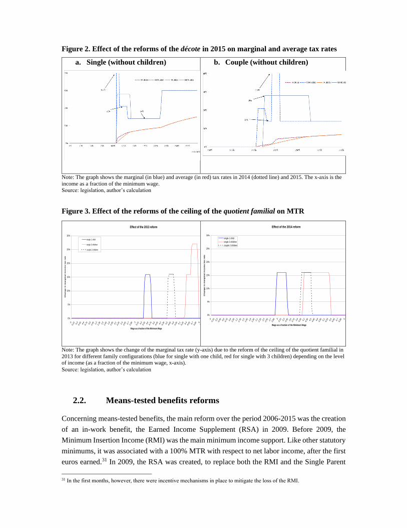
Figure 2. Effect of the reforms of the décote in 2015 on marginal and average tax rates

a. Single (without children)

b. Couple (without children)

Note: The graph shows the marginal (in blue) and average (in red) tax rates in 2014 (dotted line) and 2015. The x-axis is the

income as a fraction of the minimum wage.

Source: legislation, author’s calculation

Figure 3. Effect of the reforms of the ceiling of the quotient familial on MTR

Note: The graph shows the change of the marginal tax rate (y-axis) due to the reform of the ceiling of the quotient familial in

2013 for different family configurations (blue for single with one child, red for single with 3 children) depending on the level

of income (as a fraction of the minimum wage, x-axis).

Source: legislation, author’s calculation

2.2. Means-tested benefits reforms

Concerning means-tested benefits, the main reform over the period 2006-2015 was the creation

of an in-work benefit, the Earned Income Supplement (RSA) in 2009. Before 2009, the

Minimum Insertion Income (RMI) was the main minimum income support. Like other statutory

minimums, it was associated with a 100% MTR with respect to net labor income, after the first

euros earned.31 In 2009, the RSA was created, to replace both the RMI and the Single Parent

31 In the first months, however, there were incentive mechanisms in place to mitigate the loss of the RMI.

Effect of the 2013 reform

0%

5%

10%

15%

20%

25%

30%

00,15 0,

30,45 0,

60,75 0,

91,05 1,

21,35 1,

51,65 1,

81,95 2,

12,25 2,

42,55 2,

72,85

33,15 3,

33,45 3,

63,75 3,

94,05 4,

24,35 4,

54,65 4,

84,95 5,

15,25 5,

45,55 5,

75,85

66,15 6,

36,45 6,

66,75 6,

9

Wage as a fraction of the Minimum Wage

Ch

an

ge

in

ma

rg

ina

l in

co

me

ta

x r

ate

single 1 child

single 3 children

couple 2 children

Effect of the 2014 reform

0%

5%

10%

15%

20%

25%

30%

00,15 0,

30,45 0,

60,75 0,

91,05 1,

21,35 1,

51,65 1,

81,95 2,

12,25 2,

42,55 2,

72,85

33,15 3,

33,45 3,

63,75 3,

94,05 4,

24,35 4,

54,65 4,

84,95 5,

15,25 5,

45,55 5,

75,85

66,15 6,

36,45 6,

66,75 6,

9

Wage as a fraction of the Minimum Wage

Ch

an

ge in

marg

inal in

co

me t

ax r

ate

single 1 child

single 3 children

couple 2 children

Allowance (API) with the major difference that a rise in income from working is not cancelled

out by a fall in income from transfers: the MTR of the RSA is 38%. In concrete terms, the RSA

is composed of two parts: the basic RSA which exactly replaces the RMI with an MTR of

100%; and the RSA activité which is an employment incentive scheme whose objective is to

ensure that working more increases disposable income. The RSA activité has a negative MTR

in a first progressive zone (-62%) then a positive one in the degressive zone (+38%).

As shown in Figure 4, the reform of the RSA had a different effect on MTR according to family

configuration: for a person with an income equal to 50% of the minimum wage, the effect is

+38% on MTR if single and -62% if in a couple with a child; for a person with an income equal

to 1 minimum wage, the effect is +38% if in a couple and 5% if single; for a person with an

income equal to 150% of the minimum wage, it is +38% if in a couple without children, +7%

if in a couple with one child, and no effect if single. These heterogeneous effects depending on

family configuration will provide good sources of identification for the econometric strategy.

Finally, some family benefits were also substantially modified (see appendix A for details).

The main family benefits, “Allocations Familiales” (hereafter AF) are a family allowance for

parents of two or more children. Before 2014, this allowance was a “universal” lump sum, and

in 2015 it started to be means-tested: it was reduced by half when annual resources exceeded

67,140 euros and divided by four for incomes above 89,490 euros. There is a degressive

mechanism to mitigate the threshold effects, inducing a 100% MTR in the two degressive zones

just after the threshold.

Another family benefit was modified, leading to an increase in MTR: the “Prestation d'accueil

du Jeune Enfant” (early childhood benefit, hereafter PAJE), which is a monthly subsidy paid to

low-income families with young children. This allowance was reformed for families with a

child born after April 1, 2014. Means-testing for the basic allocation was tightened (the

thresholds were reduced). In addition, the wealthiest eligible households were now paid the

basic allowance at a reduced rate.

The amount and income ceiling of two means-tested family benefits to support low-income

families (a school allowance32 for families with one or more children aged 6 to 18, and a family

supplement for families with at least 3 children aged 6 to 18) were increased33 by more than

10% over several years. The increase of the means-tested benefit changed the level of the phase-

out by the same amount, and thus the MTR (equal to 100% in the phasing-out of the benefit).

It should be noted that family benefits affect different parts of the distribution and, as a result,

many people were affected by income tax and family benefit reforms at the same time or by

family benefit and RSA reforms at the same time.

32 “Allocation de Rentrée Scolaire”, hereafter ARS. 33 The ARS was exceptionally increased by 150 euros in 2009 and by 25% in 2012.

Figure 4. Effect of the reforms of the RSA on MTR

Source: legislation, author’s calculation

3. Data and descriptive statistics

3.1. Data

The data used are taken from the Enquêtes Revenus Fiscaux et Sociaux (hereafter ERFS), which

combine income tax records from the fiscal administration, administrative records from

organizations in charge of distributing benefits,34 and the French Labor Force Survey (hereafter

LFS). Tax data includes the annual income of each household member for year t, as well as

employees' earnings for years t, t-1 and t-2. The earnings variables are reported by employers

and are especially reliable since they are controlled by the fiscal administration with frequent

audits. Tax data also includes other income earned by the household, household size, age of

household members, marital status, and all tax return information.

Since there is limited information on individual characteristics in these administrative data, they

are matched with the LFS, which provides a great variety of socio-demographic variables.

Matching with LFS reduces the size of the data (to about 120,000 people, compared to nearly

40 million households in the tax data), but allows to simulate benefits by microsimulation (see

below) and monitor in a rich way the return to the mean and heterogeneous trends in income

distribution. In addition, as the LFS is top coded, many very high income earners are excluded

34 Caisse nationale d’allocations familiales (Cnaf), Caisse nationale d’assurance vieillesse (Cnav), and Caisse centrale de la

mutualité sociale agricole (CCMSA).

from it, and thereby from ERFS. This exclusion may actually be an advantage, as many

econometric issues in the estimation of taxable income elasticity (mean-reversion, not-tax

heterogeneous income trend, importance of capital income and income-shifting) are specific to

very high income earners.

The LFS is a rotating 18-month panel in which individuals are interviewed during six

consecutive quarters. Individuals interviewed at the 4th quarter of year t in the LFS are matched

with their year t administrative income tax records to generate the year t wave of the ERFS

dataset. Thus, one third of LFS households are present for two consecutive years in the ERFS

data set, so two ERFS can be matched to these households. I match each wave of the ERFS

between 2007 and 2015 with the previous year's (not including people moving during the

survey35), giving 9 two-year panels. These 9 panels together constitute my database of 100,668

people.

3.2. Sample used

The scope of the study is limited to people whose marital status has not changed between dates

t-1 and t, since people who marry, divorce or lose their spouses during year t have to file

different tax returns in year t. In addition, I only keep observations whose income in base-year

is more than a quarter of the annual minimum wage (around 3500 euros in 2015), since means-

reversion is very strong below this income level. Indeed, the variation of labor income along

the wage distribution is very strong below 0.25 times the annual minimum wage and much

lower thereafter (Figure A1 in Appendix B). Finally, I restrict the sample to employees who

report a positive labor income in years t−1 and t. The final sample encompasses 92,508

individuals.

In some specifications, it is necessary to use t-2 income (zi,t−2) data, which is only available for

employees. This sample of employees (self-employed excluded) encompasses 85,193

individuals.

3.3. Calculation of marginal tax rates

Since marginal (and average) tax rates are not directly observed in the data, it is necessary to

simulate them for each taxpayer. To do this, I use the micro-simulation model INES36 provided

by INSEE (French National Institute of Statistics and Economic Studies) and DREES (French

Ministry of Health and Solidarity), which I modify for the purpose of this study.37 This model

35 I checked that people kept the same characteristics (sex, age, spouse, children, marital status, etc.) to take into account any

possible moves during the survey. 36 The model INES is in open access since June 2016. A detailed description and its source code can be found on the Adullact

website (https://adullact.net/projects/ines-libre). This model has also been used by Lehmann et al. (2013) to compute ETI. 37 I modify this model in two ways for this study. First, since in the French tax schedule, the year of income taken into

account for the calculation of tax in year t is not always year t (for example, it is year t-1 for income tax), the INES model

simulates the tax schedule of year t depending on the income of year t-1 for income tax and t-2 for some benefits. To be able

to estimate equation (9), I adapt the model to simulate the tax schedule of the same year as the income. The underlying

assumption of this choice is that individuals anticipate a stable tax schedule between t and t+1 when they choose their income

in year t, and thus do not anticipate reforms in year t+1. As French income tax parameters of year t+1 are voted by the

simulates each transfer by reconstructing the appropriate unit (home, tax-household, family,

household, and so on). It provides simulated transfers very close to the levels observed in the

administrative data.

After this first step, I can compute the marginal tax rates (MTR) of each tax and benefit, by

increasing labor income by 5% for each person and comparing the modified disposable income

with that in the counterfactual scenario. For households with more than one earner, the MTR

are calculated for each income earner by increasing each income by 5% in turn. Within the

same household, MTR may be different for each person in the household (husband, wife,

student children, etc.). This is an important difference with the ETI literature, which estimates

elasticities with respect to the MNTR at the tax household level.

Finally, since tax records also provide information on the labor income at t-1 and t-2, I can

compute the different instruments of the MNTR and ANTR by taking previous years' incomes

and applying the year's inflation to them.

3.4. Descriptive statistics

Descriptive statistics of the basis for estimation are presented in Table A2 in Appendix B. It

shows that the marginal net of tax rates (MNTR) have a high standard deviation of 13 % of

labor income for income tax, 227 % for RSA and 7.1 % for family benefits. This strong

heterogeneity is also found in the annual variation of MNTR, whose standard deviation is

greater than 10% for each transfer. Table A2 also shows that the socio-demographic

characteristic of the sample reflects those of the working French population.38

Appendix B also displays the distributions of the ratio of labor income (z) to the annual

minimum wage for each year (Figure A2) and the distributions of simulated MNTR for income

tax and benefits for the different years (Figure A3). In these tables and figures, there is

variability from year to year at each point in the distribution, but it is difficult to determine

whether this heterogeneity reflects socio-demographic, income, or behavioral responses to tax

reforms. Several tax-related changes can be identified for MNTR. The lowest MNTR were in

2014, when there was a large reduction in income tax associated with a 100% MTR, and the

MNTR at the top of the distribution were lower after 2013, when the higher MTR were raised

(Figure A3.a). With regard to benefits (Figure A3.b), we clearly see the creation of the RSA in

2009, which reduced the MTR at the bottom of the distribution, and thus increased the MNTR

(and the opposite between 0.8 and 1.5 times the minimum wage in the phasing out of the RSA).

parliament at the end of income year t, it is impossible to adapt income of year t to future reforms of year t+1, and this static

policy expectation therefore seems credible. The second main change in the model concerns the take-up of the RSA benefit

schedule. Eligibility for RSA is simulated, but take-up is imputed using the social administrative data of the ERFS in this

study, and not randomly imputed as in the model INES. Indeed, in the INES model, the non take-up of certain benefits such

as the RSA is randomly imputed to achieve the administrative social data target. 38 38% had completed higher education, 75% worked in the tertiary sector, 84% worked full-time, 65% had a permanent

contract in a private company, 54% had been working in the same company for more than 10 years and 38% lived in a

municipality with a population of more than 200,000.

Reforms that have a different effect on households with the same income but different family

size39 do not show up in Figure A3, while they are an important source of identification. To get

a better idea of the source of our estimates, Table 1 shows the number of people facing a non-

zero predicted change in the MNTR of income tax and benefits (i.e., the change in the MNTR

instrument), decomposed by the magnitude of the change. This table shows, for example, that

37,557 people (about 40% of the sample) face a change in MNTR due (only) to income tax

reforms, and of these, 11,335 people (12% of the sample) face a change in their MNTR between

1% and 10%, 6,776 people face a change between 10% and 50% and 500 more than 50%.

Turning to means-tested benefits, 12,300 people face a change in the MNTR due to benefit

reforms (about 15% of the sample), nearly 2,000 face a decrease in their MNTR of more than

50%, and 1,200 face an increase of more than 50%. This heterogeneity of predicted variations

in MNTR can also be revealed by the high standard deviation of this variable in Table A2. The

many relatively large increases and decreases in the predicted variations of the MNTR are

important for econometric estimates because they imply that the tax variations used are not

systematically correlated with the level of income before the reform, which alleviate the issue

of mean reversion and heterogeneous income trend.

Table 1. Number of people facing a non-zero change in the MNTR income tax and benefit

instrument

Changes in MNTR

Income tax

Means-tested benefits

Inf. -50 % 633 1 952

-50 % à -10 % 7 541 3 383

-10 % à -1% 10 775 1 405

1 % à 10 % 11 335 1 393

10 % à 50 6 776 2 972

Sup. 50 497 1 193

Total 37 557 12 298 Reading note: 1952 people faced a decrease in benefit retention rates of more than 50% (equivalent to an increase of more than

50% in the marginal benefit rate)

Source: ERFS 2006-2015; INES model

4. Results

In all estimates, the following transfers are taken into account: income tax (IT), RSA, and family

benefits (FB) including PAJE, ARS, FC and AF.40 The reactions to MNTR are computed for

each of these transfers separately or grouped together (ALL). I first provide graphical evidence

(section 4.1), before turning to 2SLS estimation (section (4.2).

39 For instance, reform of the family quotient in Figure 3, reform of the RSA in Figure 4, or reform of family allowances. 40 They are grouped together because they do not have enough people separately. Other transfers (such as social security

contributions or housing allowances) are not taken into account because of the absence of any salient reform in the period.

4.1. Graphical evidence

I first provide graphical and semi-parametric evidence corresponding to first-stage and reduced-

form regressions. Since I use several different reforms as sources of variation, it enables me to

visualize the effect of MNTR on labor income. Indeed, unlike Kleven and Schulz who use

mainly one reform to identify the effect, I cannot use a graphical difference-in-difference to

highlight the effect.

Figures 5 and 6 plot a local fourth-order polynomial regression41 of a variable Y on a variable

X. In each graph, the gray area represents a 95% confidence interval. These graphs are based

on Weber (2014) who first used them for the ETI estimation.42 Like Weber (2014), these graphs

depict polynomial regressions for predicted MNTR between -20% and +20%, which includes

more than 90% of the sample.43

Figure 5. Delta log of the MNTR according to the delta log of its instrument (first stage)

Notes: The figure represents a fourth-order local polynomial regression of the variation of the log MNTR on the variations of

the "predicted" log MNTR. No control variables included. The smoothing parameter is 0.09 (determined with AIC).

Source: ERFS 2006-2015

41 I use the Epanechnikov kernel function for all polynomial regressions, associated with a polynomial order of four and a

bandwidth (calculated automatically by a Akaike Information Criterion (AIC)) of around 0.15 (depending on graphs). 42 Weber was not the first to use this non-parametric representation to investigate the effect of taxation: Bianchi et al. (2001)

provide graphical results of GAM (general-additive model) estimation for week work depending on tax rates to show the non-

linear effect of the pay-as-you earn reform in Iceland in 1987. Note that the graph of Weber is now commonly used in ETI

literature, for instance in Doerrenberg et al. (2017) and Hermle and Peichl (2018). 43 As Weber (2014) explains, "Extreme observations are excluded because the standard deviations on these observations are

large and make the rest of the graph difficult to read”.

A graphical illustration of the first step of the estimates in equation (9) is provided in Figure 5

for all transfers and for each separately. As expected, it shows a strong positive relationship

between the MNTR and its instrument, the predicted log change of MNTR (MNTR if incomes

were held constant). This positive relationship is almost linear for all transfers and income tax,

but less so for the RSA and family benefits (particularly at the top of the distribution of the

change of the instrument44).

Figure 6. Delta log of labor income as a function of the delta log of the predicted MNTR

(reduced form)

Notes: Graphical evidence of the reduced form of equation (9). The figure represents a fourth-order local polynomial regression

of the change in the logarithm of labor income to the changes in the logarithm of the MNTR predicted. No control variables

included. The smoothing parameter is 0.11 (determined with AIC).

Source: ERFS 2006-2015

Figure 6 provides a graphical representation of the reduced-form regressions. The relationship

between the change in the logarithm of labor income and the predicted log change of MNTR is

illustrated for all transfers, and for transfers in detail. The two variables are positively related

for all transfers, and for income tax and RSA. This reflects the positive elasticities that I estimate

econometrically in the next section and is consistent with a positive substitution effect. Since

the positive slope is steeper for income tax, the elasticity of income tax is expected to be higher

than that of benefits. For income tax, the relationship is strong for negative values and weaker

44 This may be related to the fact that there are fewer individuals and the estimates are less robust at the extremities.

for positive values, with a decrease at the top, which suggests that the effect of an increase in

MTR (and decrease in MNTR) is stronger than the opposite. The overall shape of the slope is

also positive for the RSA, but not at the beginning and top of the distribution, and the 95%

confidence interval is larger. For family benefits, the slope is almost constant (with a slight

increase above 10%) and the confidence interval is large, so the relationship does not seem

significant.

4.2. Panel Regression Evidence

In this section, I present the results of the estimation of equation (9) using the two-stage least

squares (2SLS) method. The first-stage regressions of the MNTR on its instrument (the

predicted MNTR) give significant F-statistics that are always high, meaning that the

instruments are strongly correlated with the instrumented regressors. The first-stage regressions

give very significant coefficients: above 0.5 for the direct effect of ∆logτi,tk

on ∆logτi,tk (see Table

A3 in Appendix C). The full results of equation (9) are presented in Table A4 in Appendix C.45

In all the following results, I will present the elasticity of all the transfers combined on the first

line, then the detail of the elasticity by transfers.

4.2.1. Baseline results

The baseline specification estimated in Table 2 is based on the whole sample defined in Section

3.2, using an “Auten and Caroll” (hereafter A&C) type instrument, including all covariates, and

splines of the logarithm of initial income t-1 (Gruber and Saez type, hereafter G&S) to control

for divergence in the distribution of income.

Taking into account all transfers gives a compensated elasticity with respect to MNTR of

0.086.46 Note that this is the elasticity that should be used in optimal tax formulas to calculate

optimal MTR, because it takes into account the overall tax and benefit system, while optimal

tax studies usually illustrate the formulas with elasticities estimated only with income tax

reforms.

The estimate yields a compensated elasticity of 0.26 for income tax reforms, 0.09 for RSA

reforms (in-work benefit), and not significant for other means-tested benefits (family benefits).

The differences between these elasticities47 are significant in each case, particularly between

income tax and the RSA, which contradicts the predictions of the standard labor supply model

(equation 8). The difference between the elasticity with respect to income tax and the elasticity

45 It should be noted, for example, that the coefficient on labor income at period t-1 is significantly negative, which is

consistent with the phenomenon of mean-reversion. 46 One must recall that “all transfers” relates to income tax, RSA and all family benefits. If we take into account all other

transfers (such as social security contributions, housing allowances, other social minima) and regress the labor cost on the

marginal and average effective net-of-tax rates (MENTR and AENTR) calculated with labor cost, the compensated elasticity

wrt MENTR is close to zero and elasticity wrt AENTR is -0.1. One conclusion could be that the increased complexity of the

tax and benefit system including contributions prevents individuals from knowing their METR and thus reacting to it, while

individuals are more sensitive to their AENTR. However, since there is no good source of identification to estimate the effect

of social contributions and housing allowances, these results should be taken with caution. 47 And between the elasticities divided by the average of the MNTR, as in equation (9).

with respect to benefits can be explained by the fact that income tax reforms are more visible

and salient than benefit reforms. Indeed, Chetty et al. (2009) show that consumers underreact

to taxes that are not salient. This could be related to individuals' better understanding of the

calculation of income tax and the resulting work incentives48 than of means-tested benefits. It

is consistent with the result of Bosch et al. (2019) who explain their non-bunching response to

kinks and notches in the Dutch system of cash transfers due to the lack of salience and

inattention.49

The difference between the elasticity with respect to income tax and RSA could also be related

to a compositional effect. Indeed, the beneficiaries of the RSA activité are mainly located on

the first half of the distribution while income tax mainly affects the second half, and the

elasticity seems to be higher for higher incomes. But I find that the elasticity of income tax at

the bottom of the distribution is 0.22 (Appendix C) - more than twice that of the RSA. Note that

Carbonnier (2014) finds that elasticities of income tax along the distribution are U-shaped in

France on the extensive margin, which invalidates the hypothesis of the composition effect.

Table 2. Elasticity estimates in the reference model

All transfers Detailed transfers

𝛽𝜏𝑎𝑙𝑙 0.086 ***

(0.007)

𝛽𝜌𝑎𝑙𝑙 0.255 ***

(0.016)

𝛽𝜏𝐼𝑇

0.260 ***

(0.018)

𝛽𝜏𝑅𝑆𝐴

0.090 ***

(0.009)

𝛽𝜏𝐹𝐵

-0.018

(0.016)

𝛽𝜌𝐼𝑇

0.433***

(0.026)

𝛽𝜌𝑅𝑆𝐴

0.342 ***

(0.050)

𝛽𝜌𝐹𝐵

0.065 ***

(0.018)

Observations 89122 89122 Note: Estimation of equation (9) by 2SLS using A&C instrument, G&S control of the base year income and other controls.

IT= Income Tax; RSA= In-work benefit; FB= Family Benefit; ALL= IT+RSA+ FB;

Standard errors are in round brackets. Respectively *, *** and *** indicates a significance of 10%, 5% and 1%.

Sample: employees and self-employed persons present for two consecutive years, whose labor income represents more than a

quarter of the annual minimum wage.

Source: Insee, ERFS 2006-2015

My estimate of the compensated elasticity of labor income relative to the income tax MNTR,

0.26, is within the range of the total income or labor income elasticity observed in the literature.

In the United States, many papers report total income elasticity: 0.66 for Auten and Caroll

(1999), 0.12 for Gruber and Saez (2002), 0.4 for Saez (2003), 0.2 for Saez (2004), between 0.15

48 Lardeux (2018) shows that people react to the threshold of entry into income tax using a bunching method. 49 They do not observe gradual learning, as income dynamics around the notch are not different for income intervals just

below and just above the notch, which also suggests that households are largely unaware of the threshold.

and 0.23 for Giertz (2007), an upper limit of 0.3 for Giertz (2010), 0.29 for Burns and Ziliak

(2017), and 0.48 for Weber (2014). In Scandinavian countries, broad income elasticities are

lower: 0.07-0.2 in Denmark (Kleven and Schulz, 2014), 0.02-0.05 in Norway (Thoresen and

Vatto, 2015), 0.21 for Finland (Matikka, 2017), and in Sweden 0.09-0.15 by Gelber (2014) and

0.2-1 by Blomquist and Selin (2010) for labor income. As Jongen and Stoel (2019) note: “It

appears that the elasticity of broad income in Continental European countries takes an

intermediate position between Anglo-Saxon countries and Scandinavia”: Doerrenberg et al.

(2016) estimate that the total income elasticity is 0.16 to 0.28 in Germany, while Jongen and

Stoel (2019) find 0.24 in the Netherlands. In France, Lehmann et al. (2013) find a labor income

elasticity of 0.2. This last study is the closest to ours in terms of methodology and data, and the

results are very consistent (although not using the same reforms). In his meta-analysis, Neisser

(2018) finds an average ETI estimate before deduction of 0.252 in "other countries" (other than

the United States and Scandinavia), very close to mine (0.260).

Concerning the elasticity with respect to benefits, very few points of comparison are available

because they are mainly estimated on labor force participation (extensive and non-intensive

margins). Eissa and Hoynes (1998) obtain an elasticity of 0.14 for EITC over working hours,

slightly higher than our estimate for the RSA activité. The low response to RSA reform is in

line with Briard and Sautory (2012) and Bargain and Vicard (2014) in France. The non-

significant reaction to family benefit reform might seem contradictory to other studies which

find a significant (but small) reaction in France (Piketty, 2003; Givord and Marbot, 2015), but

I estimate mainly an intensive response while these studies highlight an extensive margin

response which is not linked to a variation in MTR but to a change in the average tax rate. The

low response of benefit is in line with recent work by Bosch et al. (2019), who find a non-

bunching response to kinks and notches in the Dutch system of cash transfers.

Finally, the elasticity of the average-net-of tax rate (ANTR) is 0.43 for income tax, 0.34 for the

RSA, and 0.07 for family allowances. All these elasticities are significant, and are significantly

different from each other. Elasticities are positive, which is in apparent contradiction with the

theory that predicts a negative value if leisure is a normal good. Two explanations for this sign

can be proposed. A first explanation is based on the substitutability between time and money in

household production. An income effect can not only increase leisure (if it is a normal good50)

but also reduce domestic work (by paying an employee, for example), and thus increase the

labor supply if the latter effect dominates. This explanation was given by Bargain et al. (2014),

who also estimate a positive effect on income in some countries (Nordic countries and

Hungary). Although the majority of studies recorded low negative or zero values, it should be

noted that a number of studies also report positive elasticities51 and that Blundell and MaCurdy

(1999) report that the variability in income effects between studies is higher than that observed

on wage elasticity. My second (preferred) explanation is that this positive elasticity with respect

50 Another explanation may be that leisure may not be a normal good for some people. 51 Reported by Bargain et al. (2014), including some studies in Scandinavia, Netherlands and US.

to MTR may reveal a response along the extensive margin (participation behavior on the labor

market) and not an income effect along the intensive margin. Indeed, the average tax rate is a

proxy for the participation tax rate (calculated between non-employment and employment or

between part-time and full-time work) and, thus can have an impact on the participation rate.

For example, in the phasing-out of the RSA, the MTR is positive while the participation tax

rate and the average tax rate are negative: after its creation, a person who works at quarter time

can be incited to work half or full time because of this participation effect of the RSA that is

captured by the average tax rate. Therefore, the elasticity with respect to ATR could be

considered as a participation elasticity related to part-time work. The fact that this elasticity is

important and significant for the RSA activité, for which it is known that part-time work is

important, strengthens this idea. Carbonnier (2014) also showed a positive elasticity of labor

market participation at the participation retention rate in France for income tax. In a robustness

check (see next section), the ANTR is replaced by a participation retention rate and I obtain

positive elasticities of a comparable order of magnitude, confirming the hypothesis that the

reaction to the ANTR is partly a reaction to the participation rate along the extensive margin.

The reaction to ANTR may also actually be a reaction to MNTR because individuals tend to

approximate the MTR by the ATR, which has been shown empirically in the literature due to

the complexity of the tax and benefit system (De Bartelone, 1995; Ito, 2014; Gideon, 2015;

Rees-Jones and Taubinsky, 2016). For instance, Feldman et al. (2016) show that individuals

react by substitution effect to an ATR increase because they think it is a MTR.52

For the sake of simplicity, I will comment below mainly on the value of the compensated

elasticity with respect to the MNTR, due to the importance of this parameter in the public

economy and the difficulty in interpreting the elasticity with respect to the ANTR.

Lastly, note that since labor income does not include tax deductions53 and is less subject to

retiming phenomena than other income such as capitalized earnings and stock options

(Goolsbee, 2000), these elasticities are closer to a “real” response to taxation than ETI. But

these elasticities may be underestimated because the behavioral response to taxation may take

time and because of optimization frictions. Using Chetty’s (2012) methodology to compute the

structural elasticity in an environment with friction, the upper limit of this structural elasticity

is higher than I computed but remains far higher for income tax than for benefits.

4.2.2. Robustness checks

Robustness checks of the baseline estimate are performed in Tables 3 to 5.

In Table 3, I test the inclusion of different covariates. In column (1), the equation is estimated

without any covariates (except for controls for initial income, see Table 4 for the sensitivity

52 They show that following the loss of a young family benefit (at the child's 18th birthday), households reduce their labor

income, while an income effect should increase labor income and the substitution effect should be zero because the variation

in the marginal rate is zero. They explain this contradiction by the fact that individuals react by a substitution effect to what

they think is an MTR increase which is actually an ATR increase. They estimate an elasticity wrt ANTR of +0.3. 53 Because of these deductions, Chetty (2009) shows that the ETI is no longer a sufficient statistic and Doerrenberg et al.

(2014) have proved this empirically.

analysis of these controls). In column (2), time indicators are added, in column (3), I also add

the basic household composition covariates generally present in other studies because they are

available in tax data (e.g., sex, age and household composition) and, finally, in column (4), the

education and occupational covariates (e. g. level of education, type of occupation, size of firms,

sector of activity, etc.) specifically derived from the Labor Force Survey (and therefore rarely

used in previous studies on the subject) are added, leading to the benchmark estimates. Columns

(1) and (2) give elasticities close to those of the benchmarks but slightly higher: 0.10 for all

transfers, 0.31 for income tax and 0.11 for the RSA. The addition of the tax record covariates

reduces the coefficient to 0.9 for all transfers, 0.28 for income tax and 0.10 for the RSA; slightly

above the benchmarks of 0.086, 0.260 and 0.090 obtained with the addition of the LFS

covariates. The elasticities of family benefits are never significant.54

Table 3. Elasticities according to the covariates included

No covariate

(1)

(1)+Temporal

covariates

(2)

(2)+Tax records

covariates

(3)

(3) + LFS

covariates

(4)

𝛽𝜏𝑎𝑙𝑙 0.102 ***

(0.007)

0.102 ***

(0.007)

0.091 ***

(0.007)

0.086 ***

(0.007)

𝛽𝜌𝑎𝑙𝑙 0.286 ***

(0.017)

0.287 ***

(0.017)

0.263 ***

(0.016)

0.255 ***

(0.016)

𝛽𝜏𝐼𝑇 0.306 ***

(0.019)

0.306 ***

(0.019)

0.279 ***

(0.018)

0.260 ***

(0.018)

𝛽𝜏𝑅𝑆𝐴 0.111 ***

(0.010)

0.113 ***

(0.010)

0.098 ***

(0.009)

0.090 ***

(0.009)

𝛽𝜏𝐹𝐵 -0.034 *

(0.018)

-0.035 **

(0.018)

-0.020

(0.016)

-0.018

(0.016)

𝛽𝜌𝐼𝑇 0.528 ***

(0.028)

0.531 ***

(0.028)

0.475 ***

(0.026)

0.433***

(0.026)

𝛽𝜌𝑅𝑆𝐴 0.312 ***

(0.054)

0.315 ***

(0.054)

0.358 ***

(0.051)

0.342 ***

(0.050)

𝛽𝜌𝐹𝐵 0.066 ***

(0.020)

0.066 ***

(0.020)

0.059 ***

(0.018)

0.065 ***

(0.018)

Observations 92274 92274 89122 89122 Note: Estimation of equation (9) by 2SLS using A&C instrument, G&S control of the base year income and other controls.

IT= Income Tax; RSA= In-work benefit; FB= Family Benefit; ALL= IT+RSA+ FB;

Standard errors are in round brackets. Respectively *, *** and *** indicates a significance of 10%, 5% and 1%.

Sample: employees and self-employed people present for two consecutive years, whose labor income represents more than a

quarter of the annual minimum wage.

Source: Insee, ERFS 2006-2015

Table 4 presents a sensitivity analysis of the different specifications of the initial income

controls (i.e., in t-1, also called pre-reform income). Column 1 reproduces the reference

specification, thus including a spline (of 10 pieces) of the pre-reform income to account for the

divergence in the distribution of income as in Gruber and Saez (2002) (G&S specification

below). In column (2), there are no controls on initial income. Columns (3), (4), (5) and (6) use

54 Except in the LFS covariate-free specification, where the compensated elasticities are at the limit of significance of 10%

but with a coefficient close to zero.

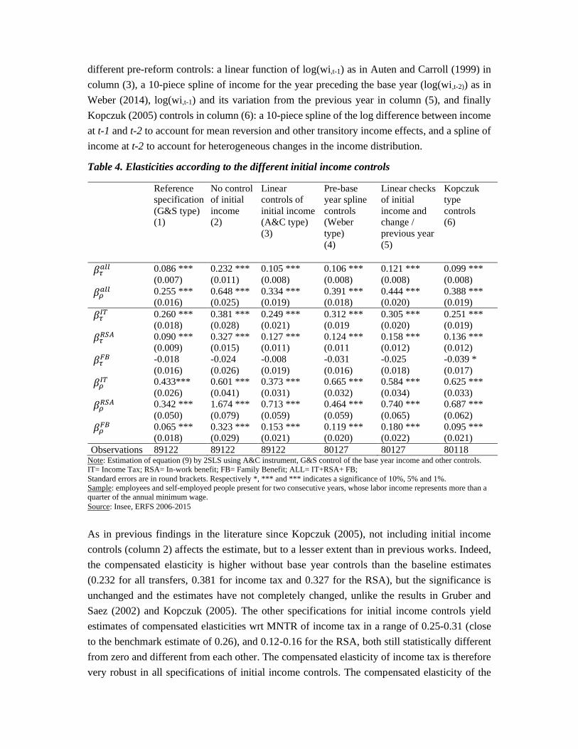
different pre-reform controls: a linear function of log(wi,t-1) as in Auten and Carroll (1999) in

column (3), a 10-piece spline of income for the year preceding the base year (log(wi,t-2)) as in

Weber (2014), log(wi,t-1) and its variation from the previous year in column (5), and finally

Kopczuk (2005) controls in column (6): a 10-piece spline of the log difference between income

at t-1 and t-2 to account for mean reversion and other transitory income effects, and a spline of

income at t-2 to account for heterogeneous changes in the income distribution.

Table 4. Elasticities according to the different initial income controls

Reference

specification

(G&S type)

(1)

No control

of initial

income

(2)

Linear

controls of

initial income

(A&C type)

(3)

Pre-base

year spline

controls

(Weber

type)

(4)

Linear checks

of initial

income and

change /

previous year

(5)

Kopczuk

type

controls (6)

𝛽𝜏𝑎𝑙𝑙 0.086 ***

(0.007)

0.232 ***

(0.011)

0.105 ***

(0.008)

0.106 ***

(0.008)

0.121 ***

(0.008)

0.099 ***

(0.008)

𝛽𝜌𝑎𝑙𝑙 0.255 ***

(0.016)

0.648 ***

(0.025)

0.334 ***

(0.019)

0.391 ***

(0.018)

0.444 ***

(0.020)

0.388 ***

(0.019)

𝛽𝜏𝐼𝑇 0.260 ***

(0.018)

0.381 ***

(0.028)

0.249 ***

(0.021)

0.312 ***

(0.019

0.305 ***

(0.020)

0.251 ***

(0.019)

𝛽𝜏𝑅𝑆𝐴 0.090 ***

(0.009)

0.327 ***

(0.015)

0.127 ***

(0.011)

0.124 ***

(0.011

0.158 ***

(0.012)

0.136 ***

(0.012)

𝛽𝜏𝐹𝐵 -0.018

(0.016)

-0.024

(0.026)

-0.008

(0.019)

-0.031

(0.016)

-0.025

(0.018)

-0.039 *

(0.017)

𝛽𝜌𝐼𝑇 0.433***

(0.026)

0.601 ***

(0.041)

0.373 ***

(0.031)

0.665 ***

(0.032)

0.584 ***

(0.034)

0.625 ***

(0.033)

𝛽𝜌𝑅𝑆𝐴 0.342 ***

(0.050)

1.674 ***

(0.079)

0.713 ***

(0.059)

0.464 ***

(0.059)

0.740 ***

(0.065)

0.687 ***

(0.062)

𝛽𝜌𝐹𝐵 0.065 ***

(0.018)

0.323 ***

(0.029)

0.153 ***

(0.021)

0.119 ***

(0.020)

0.180 ***

(0.022)

0.095 ***

(0.021)

Observations 89122 89122 89122 80127 80127 80118 Note: Estimation of equation (9) by 2SLS using A&C instrument, G&S control of the base year income and other controls.

IT= Income Tax; RSA= In-work benefit; FB= Family Benefit; ALL= IT+RSA+ FB;

Standard errors are in round brackets. Respectively *, *** and *** indicates a significance of 10%, 5% and 1%.

Sample: employees and self-employed people present for two consecutive years, whose labor income represents more than a

quarter of the annual minimum wage.

Source: Insee, ERFS 2006-2015

As in previous findings in the literature since Kopczuk (2005), not including initial income

controls (column 2) affects the estimate, but to a lesser extent than in previous works. Indeed,

the compensated elasticity is higher without base year controls than the baseline estimates

(0.232 for all transfers, 0.381 for income tax and 0.327 for the RSA), but the significance is

unchanged and the estimates have not completely changed, unlike the results in Gruber and

Saez (2002) and Kopczuk (2005). The other specifications for initial income controls yield

estimates of compensated elasticities wrt MNTR of income tax in a range of 0.25-0.31 (close

to the benchmark estimate of 0.26), and 0.12-0.16 for the RSA, both still statistically different

from zero and different from each other. The compensated elasticity of income tax is therefore

very robust in all specifications of initial income controls. The compensated elasticity of the

RSA is a little less robust: the addition of pre-reform controls increases the elasticity but does

not affect the significance of the coefficient. The elasticity of family allowances is never

significant for all specifications (as in the baseline estimate), and the elasticities with respect to

MNTR are not very far from the baseline results. The greater robustness of these results

compared with the studies on US data can be explained by four factors:

(i) In France, the distribution of labor income was very stable during the period on which this

study focuses55 (Figure A4 in Appendix B), which limits the risk that non-tax changes affect

identification. This is not the case in the United States, where the increase in pre-tax income

was particularly strong (Piketty et al., 2018).

(ii) The control of non-tax changes in income is particularly important when identification relies

on tax reforms that affect different income groups differently (the very wealthy for example, in

most US studies - see Kopczuk, 2005 and Weber, 2014). Since the reforms considered here

target different income groups and result in MTR changes that go in different directions

(increasing and decreasing, see above), the tax changes used are not systematically correlated

to the level of income before reforms, which reduces problems in identifying responses to tax

reforms (Saez et al., 2012; Lehmann et al., 2013; Kleven and Schulz, 2014).

(iii) The mean reversion is generally concentrated on the very low (see Figure A1) and very

high incomes (Guillot, 201856). Since I eliminate very low incomes and the data include few

very high incomes (see data section), this problem should be mitigated.

(iv) The socio-demographic and labor market data of the ERFS allow us to have good control

variables, which tends to minimize identification problems.

Table 5 presents the robustness checks for the instrumentation. Column 1 reproduces the

reference specification (i.e., with the classic Auten and Carroll instrument, denoted A&C below

in the tables) but on the same field as the following columns,57 which leads to slightly higher

elasticities than in Table 2. In column (2), the Weber type instrument is added to the A&C type

instrument, and column (3) uses only the Weber type instrument. Elasticity estimates are robust

across different instruments used. The elasticity of labor income with respect to the MNTR is

similar with both A&C and Weber instruments (column 2) for all transfers (0.09) and slightly

higher with the Weber instrument (0.12, column 3). The income tax elasticity is slightly higher

(0.34 versus 0.30) with the Weber type instrument but similar when the two instruments are

used together, and RSA elasticity is very close in each specification. It should be noted that on

the one hand, the Weber type instrument is supposed to be less endogenous (which reduces the

bias of the estimate), but on the other hand, it is also weaker (which reduces accuracy - see

Aronsson et al., 2017). The elasticities of family benefits are not significant in any specification,

as in the reference specification.

55 The share of the highest 0.1% has increased in France in recent decades (Garbinti et al., 2018) but as these individuals are

missing from my database, this is not a problem for the estimate. 56 Guillot (2018) shows that Gruber and Saez and Weber's method is not robust for very very high incomes (millionaires in her

case), probably because of the problem of mean-reversion. 57 Indeed, the other instruments require income in t-2 and only wage income is available at t-2.

Table 5. Elasticities for different instruments

Reference

specification

(on the same

field as (3))

(1)

A&C and Weber

type

(2)

Weber type

(3)

𝛽𝜏𝑎𝑙𝑙 0.090 ***

(0.007)

0.090 ***

(0.008)

0.119 ***

(0.009)

𝛽𝜌𝑎𝑙𝑙 0.337 ***

(0.017)

0.431 ***

(0.021)

0.332 ***

(0.015)

𝛽𝜏𝐼𝑇 0.297 ***

(0.017)

0.292 ***

(0.018)

0.344 ***

(0.020)

𝛽𝜏𝑅𝑆𝐴 0.094 ***

(0.010)

0.097 ***

(0.011)

0.108 ***

(0.014)

𝛽𝜏𝐹𝐵 -0.029

(0.017)

-0.004

(0.015)

0.011

(0.017)

𝛽𝜌𝐼𝑇 0.686 ***

(0.029)

0.823 ***

(0.036)

0.702 ***

(0.028)

𝛽𝜌𝑅𝑆𝐴 0.312 ***

(0.054)

0.309 ***

(0.064)

0.220 ***

(0.053)

𝛽𝜌𝐹𝐵 0.068 ***

(0.019)

0.145 ***

(0.023)

0.113 ***

(0.017)

Observations 80117 79882 80012 Note: Estimation of equation (9) by 2SLS using A&C instrument, G&S control of the base year income and other controls.

IT= Income Tax; RSA= In-work benefit; FB= Family Benefit; ALL= IT+RSA+ FB;

Standard errors are in round brackets. Respectively *, *** and *** indicates a significance of 10%, 5% and 1%.

Sample: employees and self-employed people present for two consecutive years, whose labor income represents more than a

quarter of the annual minimum wage.

Source: Insee, ERFS 2006-2015

In Appendix C, other robustness checks are implemented (Tables A5-A8). Table A5 tests the

robustness of the specification of the ANTR, since our specification (based on Lehmann et al.,

2013) differs from the main articles on the subject (which either do not include the effect on

income, or use the Gruber and Saez specification). The elasticity with respect to MNTR is very

robust to these changes. For all transfers, the elasticity is fairly similar to the basic

specification.58 Thus, I test a specification where the ANTR is replaced by a participation

retention rate. The latter is calculated by dividing each person's wage by 2, which corresponds

either to a change to part-time work or to unemployment.59 This specification gives slightly

higher elasticity for all transfers (0.12 versus 0.9) and slightly lower elasticity for income tax

(0.20 versus 0.26). The other elasticities are very close to the basic elasticities. The elasticities

with respect to the ANTR change logically a little more (0.51 versus 0.41 for income tax), but

the significance of the coefficients does not change. The elasticities with respect to the

participation retention rate are positive, as are the elasticities with respect to the ANTR, and of

58 The specification without ANTR produces a slightly higher (but not significantly different) compensated income tax

elasticity. 59 Assuming that the unemployment benefit corresponds to 50% of the last salary. The unemployment benefit corresponds

rather to about 60% of the last salary, but the results would be very similar if a rate of 60% had been used.

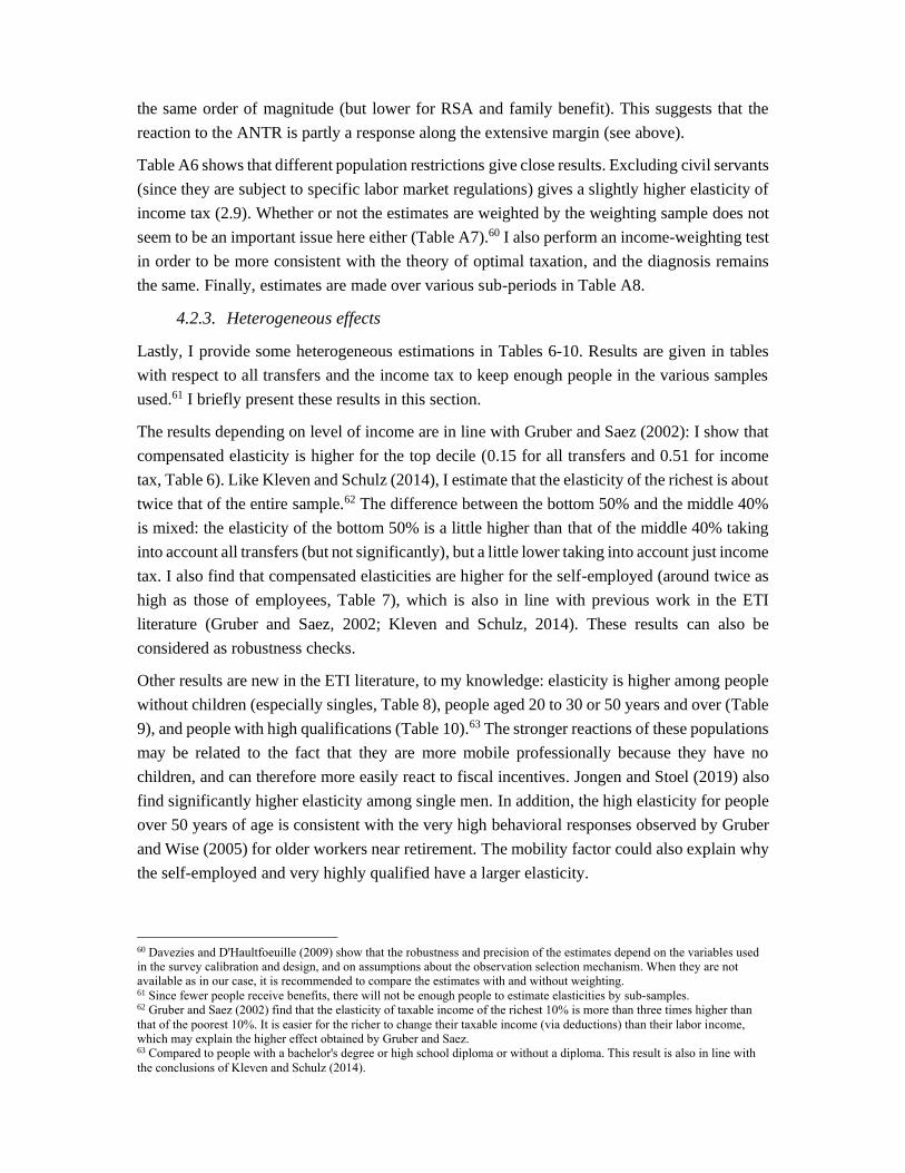
the same order of magnitude (but lower for RSA and family benefit). This suggests that the

reaction to the ANTR is partly a response along the extensive margin (see above).

Table A6 shows that different population restrictions give close results. Excluding civil servants

(since they are subject to specific labor market regulations) gives a slightly higher elasticity of

income tax (2.9). Whether or not the estimates are weighted by the weighting sample does not

seem to be an important issue here either (Table A7).60 I also perform an income-weighting test

in order to be more consistent with the theory of optimal taxation, and the diagnosis remains

the same. Finally, estimates are made over various sub-periods in Table A8.

4.2.3. Heterogeneous effects

Lastly, I provide some heterogeneous estimations in Tables 6-10. Results are given in tables

with respect to all transfers and the income tax to keep enough people in the various samples

used.61 I briefly present these results in this section.

The results depending on level of income are in line with Gruber and Saez (2002): I show that

compensated elasticity is higher for the top decile (0.15 for all transfers and 0.51 for income

tax, Table 6). Like Kleven and Schulz (2014), I estimate that the elasticity of the richest is about

twice that of the entire sample.62 The difference between the bottom 50% and the middle 40%

is mixed: the elasticity of the bottom 50% is a little higher than that of the middle 40% taking

into account all transfers (but not significantly), but a little lower taking into account just income

tax. I also find that compensated elasticities are higher for the self-employed (around twice as

high as those of employees, Table 7), which is also in line with previous work in the ETI

literature (Gruber and Saez, 2002; Kleven and Schulz, 2014). These results can also be

considered as robustness checks.

Other results are new in the ETI literature, to my knowledge: elasticity is higher among people

without children (especially singles, Table 8), people aged 20 to 30 or 50 years and over (Table

9), and people with high qualifications (Table 10).63 The stronger reactions of these populations

may be related to the fact that they are more mobile professionally because they have no

children, and can therefore more easily react to fiscal incentives. Jongen and Stoel (2019) also

find significantly higher elasticity among single men. In addition, the high elasticity for people

over 50 years of age is consistent with the very high behavioral responses observed by Gruber

and Wise (2005) for older workers near retirement. The mobility factor could also explain why

the self-employed and very highly qualified have a larger elasticity.

60 Davezies and D'Haultfoeuille (2009) show that the robustness and precision of the estimates depend on the variables used

in the survey calibration and design, and on assumptions about the observation selection mechanism. When they are not

available as in our case, it is recommended to compare the estimates with and without weighting. 61 Since fewer people receive benefits, there will not be enough people to estimate elasticities by sub-samples. 62 Gruber and Saez (2002) find that the elasticity of taxable income of the richest 10% is more than three times higher than

that of the poorest 10%. It is easier for the richer to change their taxable income (via deductions) than their labor income,

which may explain the higher effect obtained by Gruber and Saez. 63 Compared to people with a bachelor's degree or high school diploma or without a diploma. This result is also in line with

the conclusions of Kleven and Schulz (2014).

Table 6. Elasticities according to level of labor income

Total

population

(1)

50% from the

bottom

(2)

40% of the

middle

(3)

Top 10%

(4)

all

0.086 ***

(0.007)

0.083 ***

(0.009)

0.067 ***

(0.013)

0.153 **

(0.061)

𝛽𝜌𝑎𝑙𝑙 0.247 ***

(0.016)

0.201 ***

(0.021)

0.452 ***

(0.028)

0.307 ***

(0.060) IT

0.260 ***

(0.018)

0.222 ***

(0.024)

0.332 ***

(0.025)

0.508 ***

(0.100) IT

0.433***

(0.026)

0.409 ***

(0.043)

0.562 ***

(0.034)

0.264 ***

(0.063)

Observations 76549 44278 36260 8584 Note: Estimation of equation (9) by 2SLS using A&C instrument, G&S control of the base year income and other controls.

IT= Income Tax; ALL= IT+RSA+ FA;

Standard errors are in round brackets. Respectively *, *** and *** indicates a significance of 10%, 5% and 1%.

Sample: employees and self-employed people present for two consecutive years, whose labor income represents more than a

quarter of the annual minimum wage.

Source: Insee, ERFS 2006-2015

Table 7. Elasticities according to activity status

Employees

(1) Self-employed

(2) all

0.086 ***

(0.007)

0.122

(0.104)

𝛽𝜌𝑎𝑙𝑙 0.258 ***

(0.016)

0.158 *

(0.085) IT

0.296 ***

(0.020)

0.426 **

(0.216) IT

0.551 ***

(0.031)

0.117

(0.092)

Observations 85442 2898 Note: Estimation of equation (9) by 2SLS using A&C instrument, G&S control of the base year income and other controls.

IT= Income Tax; ALL= IT+RSA+ FA;

Standard errors are in round brackets. Respectively *, *** and *** indicates a significance of 10%, 5% and 1%.

Sample: employees and self-employed people present for two consecutive years, whose labor income represents more than a

quarter of the annual minimum wage.

Source: Insee, ERFS 2006-2015

Table 8. Elasticities according to family composition

Single

without

children

(1)

Single with

children

(2)

Couple

without

children

(3)

Couple with

children

(4)

all

0.327 ***

(0.042)

0.091 *

(0.056)

0.125 ***

(0.022)

0.044 ***

(0.013)

𝛽𝜌𝑎𝑙𝑙 0.901 ***

(0.064)

0.233

(0.074)

0.374 ***

(0.046)

0.171 ***

(0.026) IT

0.531 ***

(0.052)

0.122

(0.105)

0.270 ***

(0.038)

0.165 ***

(0.027) IT

1.073 ***

(0.087)

1.648 *

(0.223)

0.370 ***

(0.049)

0.384 ***

(0.039)

Observations 12018 2318 19184 29632 Note: Estimation of equation (9) by 2SLS using A&C instrument, G&S control of the base year income and other controls.

IT= Income tax; all=all transfers taken into account

Standard errors are in round brackets. Respectively *, *** and *** indicates a significance of 10%, 5% and 1%.

Sample: employees and self-employed people present for two consecutive years, whose labor income represents more than a

quarter of the annual minimum wage.

Source: ERFS 2006-2015

Table 9. Elasticities by age

20/30

(1) 30/40

(2) 40/50

(3) 50/60

(4) all

0.135 ***

(0.017)

0.036 ***

(0.013)

0.049 ***

(0.011)

0.065 ***

(0.016)

𝛽𝜌𝑎𝑙𝑙 0.061

(0.052)

0.297 ***

(0.029)

0.165 ***

(0.022)

0.459 ***

(0.038) IT

0.275 ***

(0.051)

0.253 ***

(0.035)

0.180 ***

(0.030)

0.300 ***

(0.031) IT

0.770 ***

(0.143)

0.541 ***

(0.051)

0.074 **

(0.036)

0.584 ***

(0.048)

Observations 10319 20276 27769 25643 Note: Estimation of equation (9) by 2SLS using A&C instrument, G&S control of the base year income and other controls.

IT= Income tax; all=all transfers taken into account

Standard errors are in round brackets. Respectively *, *** and *** indicates a significance of 10%, 5% and 1%.

Sample: employees and self-employed people present for two consecutive years, whose labor income represents more than a

quarter of the annual minimum wage.

Source: ERFS 2006-2015

Table 10. Elasticities by level of education (highest qualification obtained, from LFS variable)

College (>2

year)

(1)

College

(<=2 year)

(2)

High school

graduate

(3)

High-

school

drop-out

or

vocational

diploma

(4)

Junior high

school, no

diploma or

elementary

school

(5)

all

0.127 ***

(0.022)

0.077 ***

(0.016)

0.073 ***

(0.016)

0.082 ***

(0.010)

0.050 **

(0.023)

𝛽𝜌𝑎𝑙𝑙 0.209 ***

(0.038)

0.180 ***

(0.033)

0.392 ***

(0.043)

0.297 ***

(0.025)

0.226 ***

(0.053) IT

0.237 ***

(0.047)

0.184 ***

(0.038)

0.283 ***

(0.041)

0.278 ***

(0.027)

0.195 ***

(0.067) IT

0.232 ***

(0.043)

0.332 ***

(0.045)

0.712 ***

(0.086)

0.765 ***

(0.057)

1.440 ***

(0.175)

Observations 17174 16948 15428 33743 5508 Note: Estimation of equation (9) by 2SLS using A&C instrument, G&S control of the base year income and other controls.

IT= Income tax; all=all transfers taken into account

Standard errors are in round brackets. Respectively *, *** and *** indicates a significance of 10%, 5% and 1%.

Sample: employees and self-employed people present for two consecutive years, whose labor income represents more than a

quarter of the annual minimum wage.

Source: ERFS 2006-2015

Conclusion

In this paper, I estimate different compensated elasticities of labor income with respect to

marginal net-of-tax rate according to the type of transfer, using reforms implemented in France

between 2006 and 2015. I find elasticities of 0.2-0.3 for income tax reforms, 0.1 for in-work

benefit reforms, and not significant for family benefit reforms. Taking into account all reforms

leads to an elasticity of 0.1. These results are robust to several robustness checks. The main

contribution of this paper is to jointly estimate responses to income tax and means-tested benefit

reforms in a unique framework and with same data, and to be able to compare elasticities. I find

significantly different elasticities depending on transfers, which contradicts the prediction of

the classical labor supply model. The different behavioral responses between transfers could be

explained by the fact that income tax reforms are more salient than benefit reforms (particularly

family benefits), and that work incentives from the income tax schedule are better understood.

They could also be explained by adjustment costs and short-term optimization frictions (such

as job search costs, or costs of paying attention to tax reforms, see Chetty et al, 2011; Chetty,

2012), misperceptions of the tax and benefit system (Gideon, 2015; Rees-Jones and Taubinsky,

2016) and the difficulty of knowing the true marginal tax rate due to the limited rationality of

agents (De Bartolone, 1995; Ito, 2014). I obtain higher elasticities for top incomes, the self-

employed, young people, people without children, and people with high qualifications.

All these results have several implications and applications. Firstly, a consequence of the higher

behavioral response to income tax than to benefits is that benefit reforms can be more effective

in reducing inequalities than income tax, which is consistent with the findings of Doerrenberg

and Peichl (2014). For example, a reduction in family allowances (leading to an increase in

marginal tax rates) could be more effective in reducing inequalities or the budget deficit than

an increase in the income tax rate, since reaction to labor incomes is smaller.64 Secondly, the

estimated elasticities can also be used for normative analysis, to calculate optimal marginal tax

rates (Saez, 2001), or social preferences "revealed by the tax-benefit system" (Bargain et al.,

2013). Thirdly, these elasticities can be used to assess the distributive effects of public policies

and their effect on state budgets. For these last two purposes, it is important to use

heterogeneous elasticities by types of people (Jacquet and Lehmann, 2020) which I highlight in

this paper.

References

Aghion, P., Ciornohuz, V., Gravoueille M., & Stantcheva, S. (2019). Reforms and Dynamics

of Income: Evidence Using New Panel Data. Working Paper

Alstadsæter, A. & Wangen, K. (2010). Small Corporations’ Income Shifting through Choice of

Ownership Structure - a Norwegian Case. Finnish Economic Papers, 23(2), 73–87.

Alstadsæter, A. & Martin, J. (2016). Dividend Taxes and Income Shifting. Scandinavian

Journal of Economics, 118(4), 693–717

Angrist, J., Imbens, G. W. & Rubin, D. (1996). Identification of causal effects using

instrumental variables. Journal of the American Statistical Association, 91(434), 444–455

Aronsson, T., Jenderny, K., & Lanot, G. (2017). The quality of the estimators of the ETI.

Working Paper

Auten, G. & Carroll, R. (1999). The effect of income taxes on household behavior. Review of

Economics and Statistics, 81(4), 681-693.

Bach, L., Bozio, A., Fabre, B., Guillouzouic, A., Leroy, C., & Malgouyres, C. (2019). Follow

the money! Combining household and firm-level evidence to unravel the tax elasticity of

dividend. PSE Working paper n° 2019 – 70.

Bargain, O., & Peichl, A. (2013). Steady-State Labor Supply Elasticities: A Survey. ZEW

Discussion Paper n° 13-084.

Bargain, O. & Vicard, A. (2014). Le RMI et son successeur le RSA découragent-ils certains

jeunes de travailler ? Une analyse sur les jeunes autour de 25 ans. Economie et statistique, 467–

468, 61–69.

Bargain, O., Dolls, M., Peichl, A., Neumann, D., & Siegloch S. (2013). Tax-Benefit Revealed

Social Preferences in Europe and the US. Annals of Economics and Statistics, 113/114, 257-

289

64 We can apply this conclusion to recent French reforms: the reform of family allowances in 2014 (leading to an increase in

marginal tax rates), which aimed to reduce inequalities (and reduce the deficit), would have had small effects on labor

incomes given the estimated elasticities, unlike the increase in income taxes in 2011, 2012 and 2014, and would therefore

have been more effective in reducing inequality and the government deficit.

Bianchi, M., Gudmundsson, B. R., & Zoega, G. (2001). Iceland's Natural Experiment in Supply

Side Economics. The American Economic Review, 91(5), 1564-1579

Blomquist, S. & Selin, H. (2010). Hourly Wage Rate and Taxable Labor Income

Responsiveness to Changes in Marginal Tax Rates. Journal of Public Economics, 94, 878–889.

Blundell, R.W. & MaCurdy, T. (1999). Labor supply: a review of alternative approaches. in (O.

Ashenfelter & D. Card, eds.), Handbook of Labor Economics, vol. 3A, Elsevier.

Boissel, C., & Matray, A. (2019). Higher Dividend Taxes, No Problem! Taxing Entrepreneurs

in France. Presentation at NBER corporate finance, 2019.

Bosch, N., Jongen, E., Leenders, W. & Möhlmann, J. (2019). Non-bunching at kinks and

notches in cash transfers in the Netherlands. International Tax and Public Finance, 26(6), 1329-

1352.

Briard, P. & Sautory, O. (2012). Évaluation de l’impact du revenu de solidarité active sur l’offre

de travail. Dares, Document d’études, n° 171.

Burns, S. K. & Ziliak, J. P. (2015). Identifying the Elasticity of Taxable Income. The economic

journal, Vol. 127 (600), pp. 297-329.

Cabannes, PY, Houdré, C. & Landais, C. (2014). Comment le revenu imposable des ménages

aisés réagit-il à sa taxation ? Une estimation sur la période 1997-2004. Economie et Statistique,

467–468, 141–162.

Causa, O. & Hermansen, M. (2017). Income redistribution through taxes and transfers across

OECD countries. OECD Economics Department Working Papers, No. 1453.

Chetty, R. (2009). Is the Taxable Income Elasticity Sufficient to Calculate Deadweight Loss?

The Implications of Evasion and Avoidance. American Economic Journal: Economic Policy,

Vol 1 (2) pp. 31-52.

Chetty, R., Looney, A. & Kroft, K. (2009). Salience and Taxation: Theory and Evidence.

American Economic Review, 99(4): 1145-1177.

Chetty, R., Friedman J., Olsen T., & L. Pistaferri (2011). Adjustment Costs, Firm Responses,

and Micro vs. Macro Labor Supply Elasticities: Evidence from Danish Tax Records. Quarterly

Journal of Economics 126(2): 749-804.

Chetty, R. (2012). Bounds on Elasticities with Optimization Frictions: A Synthesis of Micro

and Macro Evidence on Labor Supply. Econometrica, 80, 969–1018.

Creedy, J., & Gemmell, N. (2019). The elasticity of taxable income of individuals in couples.

International Tax and Public Finance, 20(6), 974-991.

Davezies, L. & D’Haultfoeuille, X. (2009). Faut-il pondérer ?... Ou l'éternelle question de

l'économètre confronté à des données d’enquête. Insee working paper n°2009-06.

De Bartolome, C. A. M. (1995). Which Tax Rate do People Use: Average or Marginal? Journal

of Public Economics, 56 (1), 79–96.

Doerrenberg, P. & Peichl, A. (2014). The impact of redistributive policies on inequality in

OECD countries. Applied Economics, 46(17), 2066–2086

Doerrenberg P., Peichl A. & Siegloch, S. (2017). The elasticity of taxable income in the

presence of deduction possibilities. Journal of Public Economics, 151©, 41-55.

Eissa, N., & Hoynes, H. (1998). The Earned Income Tax Credit and the Labor Supply of

Married Couples. Working Paper 6856, NBER.

Evers, M., R. de Mooij, & D. van Vuuren (2008). The wage elasticity of Labor supply: a

synthesis of empirical estimates. De Economist, 156:25.43

Feldman, N. E., P. Katuščák, & L. Kawano (2016). Taxpayer Confusion: Evidence from the

Child Tax Credit. American Economic Review, 106 (3): 807-35.

Feldstein, M. (1995). The Effect of Marginal Tax Rates on Taxable Income: A Panel Study of

the 1986 Tax Reform Act. Journal of Political Economy, 103, 551–572.

Garbinti, B., Goupille-Lebret, J., & Piketty, T. (2018). Income Inequality Dynamics in France

1900-2014: Evidence from Distributional National Accounts (DINA). Journal of Public

Economics, 162(C), 63-77.

Gelber, A. (2014). Taxation and the Earnings of Husbands and Wives: Evidence from Sweden.

Review of Economics and Statistics. 96(2), 287-305

Gideon, M. (2015). Do Individuals Perceive Income Tax Rates Correctly? Public Finance

Review, 2015.

Giertz, S. H. (2007). The Elasticity of Taxable Income over the 1980s and 1990s. National Tax

Journal, 60(4): 743–68.

Giertz, S. H. (2010). The Elasticity of Taxable Income during the 1990s: New Estimates and

Sensitivity Analyses. Southern Economic Journal, 77(2): 406–33.

Givord, P. & Marbot, C. (2015). Does the cost of child care affect female labor market

participation? An evaluation of a French reform of childcare subsidies. Labour Economics, 36:

99-111.

Goolsbee, A. (2000). What happens when you tax the rich? Evidence from executive

compensation. Journal of Political Economy 108 (2), 352–378

Gordon, R. H., & Slemrod, J. (2000). Are ‘Real’ Responses to Taxes Simply Income Shifting

between Corporate and Personal Tax Bases? In Does Atlas Shrug? The Economic

Consequences of Taxing the Rich, edited by Joel Slemrod, 240–80. Harvard University Press.

Guillaud, E., Olckers, M., & Zemmour, M. (2019). Four levers of redistribution: The impact of

tax and transfer systems on inequality reduction. Review of Income and Wealth.

Guillot, M. (2018). Who paid the 75% tax on millionaires? Optimisation of salary incomes and

incidence in France. Working paper.

Gruber, J. & Saez, E. (2002). The elasticity of taxable income: evidence and implications.

Journal of Public Economics, 84, 1–32

Gruber, J. & D. A. Wise (2005). Social Security Programs and Retirement around the World:

Fiscal Implications of Reform. National Bureau of Economic Research Working Paper No.

11290.

Harju, J. & T. Matikka (2016). The elasticity of taxable income and income-shifting: what is

real and what is not? International Tax and Public Finance, 23, 640–669.

Hausman, J.A. (1985). The Econometrics of Nonlinear Budget Sets. Econometrica, 53, 1255–

1282.

Hermle, J. & Peichl, A. (2018). Jointly Optimal taxes for Different Types of Income. Working

paper

Ito, K. (2014). Do Consumers Respond to Marginal or Average Price? Evidence from Nonlinear

Electricity Pricing. American Economic Review, 104 (2), 537–63.

Jacquet, L. & Lehmann, E. (2020). Optimal Income Taxation with Composition Effects.

Journal of European Economic Association (forthcoming).

Jongen, E.L.W. & Stoel, M. (2019). The Elasticity of Taxable Labour Income in the

Netherlands, De Economist 167(4), 359–386.

Keane, M.P. (2011). Labor Supply and Taxes: A Survey. Journal of Economic Literature, 49,

961–1075.

Kleven, H.J. & Schulz, E.A. (2014). Estimating Taxable Income Responses using Danish Tax

Reforms. American Economic Journal: Economic Policy 6.4 (2014), pp. 271-301

Kopczuk, W. (2005). Tax bases, tax rates and the elasticity of reported income. Journal of

Public Economics, 89(11-12), 2093–2119.

Lardeux, R. (2018). Who understands the French Income Tax ? Bunching where Tax Liabilities

start. Insee working paper G2018/04.

Lefebvre, M-N, Lehmann, E., & Sicsic, M. (2019). Évaluation de la mise au barème des revenus

du capital. CRED working paper 2019-25.

Lehmann, E., Marical, F., & Rioux, L. (2013). Labor income responds differently to income-

tax and payroll-tax reforms. Journal of Public Economics, vol. 99, 66–84.

Matikka, T. (2018). Elasticity of Taxable Income: Evidence from Changes in Municipal Income

Tax Rates in Finland. Scandinavian Journal of Economics, 120(3), 943–973.

Neisser, C., (2018). The Elasticity of Taxable Income: A Meta-Regression Analysis. IZA

Discussion Papers 11958.

Pacifico, A. (2019). The lowering of the family quotient. mimeo

Piketty, T. (1999). Les hauts revenus face aux modifications des taux marginaux supérieurs de

l’impôt sur le revenu en France. Économie & Prevision, 138-139, 25–60

Piketty, T. (2003), L’impact de l’allocation parentale d’éducation sur l’activité féminine et la

fécondité. CEPREMAP, Working Papers.

Piketty, T., Saez E., & Zucman, G. (2018). Distributional National Accounts: Methods and

Estimates for the United States. The Quarterly Journal of Economics, 133(2), 553–60.

Pirttilä, J., & Selin, H. (2011). Income Shifting within a Dual Income Tax System : Evidence

from the Finnish Tax Reform of 1993. The Scandinavian Journal of Economics.

Rees-Jones, A., & Taubinsky, D. (2016). “Heuristic Perceptions of the Income Tax: Evidence

and Implications for Debiasing”. NBER Working Paper No. 22884.

Romanov, D. (2006). The corporation as a tax shelter: Evidence from recent Israeli tax changes.

Journal of Public Economics, 90(10–11).

Saez, E. (2001). Using Elasticities to Derive Optimal Income Tax Rates. Review of Economic

Studies, 68(1), 205–229.

Saez, E. (2003). The Effect of Marginal Tax Rates on Income: A Panel Study of ‘Bracket Creep.

Journal of Public Economics, 87(5–6), 1231–58

Saez, E. (2004). “Reported Incomes and Marginal Tax Rates, 1960-2000: Evidence and Policy

Implications." in James Poterba, ed., Tax Policy and the Economy, 18, 117–174.

Saez, E., Slemrod, J., & Giertz, S. (2012). The elasticity of taxable income with respect to

marginal tax rates: A critical review. Journal of Economic Literature, 50(1), 3–50.

Sicsic, M. (2018). Financial Incentives to Work in France between 1998 and 2014. Economie

et Statistique / Economics and Statistics, 503-504, 13–35.

Slemrod, J. (1996). High income families and the tax changes of the 1980s: the anatomy of

behavioral response. In: Feldstein, M., Poterba, J. (Eds.), Empirical Foundations of Household

Taxation. University of Chicago.

Thoresen, T. & Vattø, T. E. (2015). Validation of the discrete choice labor supply model by

methods of the new tax responsiveness literature. Labour Economics, 37(C), 38–53.

Van Soest, A. (1995). Structural Models of Family Labor Supply. A Discrete Choice Approach.

Journal of Human Resources, 30, 63–88.

Weber, C. (2014). Toward obtaining a consistent estimate of the elasticity of taxable income

using difference-in-differences. Journal of Public Economics, 117, 90–103.

Appendix A: French Legislation and reforms used

In this Appendix I give a short overview of the characteristics of income tax and main benefits

in France and I describe the reform that occurred in France during the 2006–2015 period, period

that I use as a source of identification. This paper reviews only reforms that affect marginal tax

rates (MTR) on net labor income, i.e., income tax and means-tested benefit reforms (where the

amount levied or received is a function of the individual's or household's65 labor income). It

should be noted that the income taken into account is different for each transfer:66 I do not enter

this level of detail thereafter for the sake of simplification, but these differences are fully taken

into account in the simulation of each transfer.

1. Income tax reforms

Firstly, I overview the characteristics of income tax in France and give more information on the

income tax reforms taken into account.

Income tax in France is calculated at the level of the tax household (which differs from the

usual notion of household67). This is a joint income taxation system where spousal incomes and

any income that the couple's children might have are jointly taxed along with the husband’s

income. A certain number of tax shares k is allocated to each tax household according to its

composition.68 The taxable income of all members of the tax household (noted yh) is added up

and divided by the number of tax shares to determine the taxable income per tax unit taxed the

following year (yh/k, quotient familial). It is taxed according to a traditional progressive tax

scale (function noted as TIR (...)) composed of many brackets associated with an MTR (see

Table 2). Finally, the tax on the income of the tax household (TIR) is computed by multiplying

the taxable income per tax unit by the number of tax unit k: TIR=k TSIR (yh/k). Because of the

joint taxation and application of the quotient familial, taxation diminishes the tax of households

with more dependent persons. Given the convexity of the income tax schedule TSIR(.), the

income-splitting mechanism reduces the income tax burden of households if k is larger than

one. However, there is a ceiling on the tax advantage for dependent persons linked to the

quotient familial in order to ensure that wealthy households with a large number of children

still pay income tax.

The décote system changes income MTR for the bottom of the scale. The décote is a tax

deduction for income which raises the point of entry into income tax as well as the MTR just

above. This mechanism is characterized by two parameters, S and r. Taxpayers are exempted

from taxes as long as TIR < S r /(1+r) and face a MTR multiplied by a factor 1 + r if r S/(1 + r)

< TIR < S (see Lardeux, 2018 for more details). Thus, this haircut mechanism creates a new first

65 Thus, reforms on capital income (such as the reform that affects taxation of dividends in 2013) and reforms on social security

contributions are not taken into account. 66 Depending in particular on the exemptions and the definition of the household taken into account. 67 Two people living as a couple are only considered by the administration as a tax household if they are married or bound by

a civil pact. 68 Husband and wife count as one unit, the first two dependents count as half a unit each, the third and following ones count

as one unit each.

hidden tax bracket (21 % instead of 14 % in 2014) at the beginning of the scale for single

taxpayers.

Finally, various measures supplement this income tax calculation and may have effects on

MTR: tax reductions and credits, the earned income tax credit, and the tax collection threshold.

Over the 2006–2015 period covered by this study, there were several changes in the income tax

code.

1/ First, the number of brackets and MTR were modified several times (see Table A1):

- In 2007, the number of tranches was reduced from 7 to 5 and the MTR and tax base

changed. The change in the number of tranches led to changes in the MTR for some

people close to the initial thresholds. The change in the MTR was offset by the

broadening of the tax base, with the exception of the top incomes,69 for which the upper

MTR fell from 48.1% to 40%.

- In 2012, two additional brackets (adding 3% and 4% to the top MTR) were created for

(single) people above 250,000 euros (twice that amount for couples) and 500,000 euros

(“contribution exceptionnelle sur les hauts revenus”), leading to a top MTR of 45%.

- In 2013, an additional 45% tranche was created for income above 150,000 euros. This

led to a 49% higher MTR taking into account the 2012 reform;

- In 2014, an exceptional tax reduction took place for the bottom of the distribution. This

reduction was 350 euros for a single person with a net taxable income of less than 13,795

euros. Then, between 13,795 euros and 14,144 euros (differential zone) for a single

person, when the reference tax income increased by one euro, the exceptional reduction

fell by one euro. This mechanism increased the marginal rate to 121% in the differential

zone for single people and 114% for couples (see Sicsic, 2018). A similar reform took

place in 2009;

- In 2015, the first tax bracket was removed and the parameter r of the décote was

modified (from 0.5 to 1), which consequently multiplied the MTR in the first bracket

by 2 and not by 1.5 as previously.

2/ The income tax and décote thresholds were modified (Table A1):

- Between 2011 and 2013, the income tax thresholds were not adjusted for inflation,

which generated a bracket creep (used by Saez 2003 as a source of identification). This

reform led 200,000 households to pay income tax for the first time between 2011 and

2012 and generated €20 million in additional tax revenue for the government in 2013.

- The tax thresholds for the discount increased much more than inflation in 2013, 2014

and 2015 (+9.3%, +5.5% and +11.7% for single people and +84% for couples in 2015).

As a result, and in addition to the change in parameter S, marginal tax rates were

69 This is due to the abolition of the 20% professional allowance on wage income, pensions and some non-wage labor income

and increased the tax base of other self-employed persons by 1.25%. The objective of enlargement was to improve the tax

system without changing the final level of tax rates, but since the 20% allowance was capped at €24,020 (for €133,444 of

taxable income), the reform reduced the top MTR. This reform therefore had a cost: 3.6 billion euros.

significantly affected in 2015, particularly for couples. For example, people in couples

with incomes between 2.1 and 2.7 times the minimum wage faced an MTR in 2015 that

was twice as high (see Figure 14) as in 2014 (28% VS 14%)70.

3/ The ceiling of the tax benefit linked to the family quotient was reduced in 2013 and 2014

(from 2336 euros to 2000 euros per child in 2013 and then to 1500 euros in 2014). This reform

led to different variations in the MTR for the same level of income according to family

composition and is therefore a very convincing source of identification.

4/ Overtime was exempt from income tax in 2007, and was taxed again in 2013.

5/ Finally, tax deductions and credits (e.g., for rental investment), as well as the capping of

these tax deductions (in 2009 in particular) underwent many changes.71

Table A1. Income tax parameters in France by year of legislation

settings 2006 2007 2008 2009 2010 2011 2012 2013 2014 2015

Income

tax on

income

Brackets

b1 0 0 0 0 0 0 0 0 0 0

b2 4 412 5 614 5 687 5 852 5 875 5 963 5 963 5 963 6 011 0

b3 8 667 11 198 11 334 11 673 11 720 11 896 11 896 11 896 11 991 9 690

b4 15 274 24 872 25 195 25 926 26 030 26 420 26 420 26 420 26 631 26 764

b5 24 731 66 679 67 546 69 505 69 783 70 830 70 830 70 830 71 397 71 754

b6 40 241 250 000 150 000 151 200 151 956

b7 49 624 500 000 250 000 250 000 250 000

b8 500 000 500 000 500 000

MTR

mtr1 0% 0% 0% 0% 0% 0% 0% 0% 0% 0%

mtr2 6,83% 5,5% 5,5% 5,5% 5,5% 5,5% 5,5% 5,5% 5,5% 0%

mtr3 19.14% 14% 14% 14% 14% 14% 14% 14% 14% 14%

mtr4 28.26% 30% 30% 30% 30% 30% 30% 30% 30% 30%

mtr5 37.38% 40% 40% 40% 40% 41% 41% 41% 41% 41%

mtr6 42.62% 44% 45% 45% 45%

mtr7 48.09% 45% 48% 48% 48%

mtr8 49% 49% 49%

Décote

S 0.5 0.5 0.5 0.5 0.5 0.5 0.5 0.5 0.5 1

r1 (simple) 814 828 838 862 866 878 878 960 1016 1135

r2 (torque) 814 828 838 862 866 878 878 960 1016 1870 Reading: The MTR faced by an individual is mtr2 if the taxable income is between b2 and b3.

Note that in the table, since 2012 I have added the "exceptional contribution on high incomes" (+3% above 250,000 euros

and +4% above 500.000 euros) to the top MTR for simplicity reasons but the tax base is not exactly the same.

Source: legislation, DGFIP

2. Reforms of means-tested benefits

The principle of all means-tested benefits is globally the same: a benefit is given to people with

incomes below a certain threshold. Above this threshold the benefit gradually decreases, leading

to a positive marginal tax rate in the phasing-out income range between the threshold and

70 Except for an area around 2.25 times the minimum wage, where the MTR decreases due to the "exceptional reduction" of

2014 (which led to an MTR of 114%, see above). 71 It should be noted that self-employed people were the subject of specific reforms (creation of the status of auto-

entrepreneur in 2009). These reforms are partially taken into account.

another threshold (the income level where the benefit is no longer paid72). I take into account

the benefits that were reformed between 2006 and 2015. The reform of the RSA has been

explained in the article. Here, I detail the reforms of some family benefits which were also

substantially modified:73

(i) “Allocations Familiales” (family allowances, hereafter AF) is a family allowance for parents

of two or more children. Before 2014, this allowance was a “universal” lump sum and was very

popular: 5 million families in France received AF. In 2015, means testing was introduced for

this allowance: it was reduced by half for annual resources exceeding 67,140 euros and divided

by four for incomes above 89,490 euros. There is a degressive mechanism to mitigate the

threshold effects, inducing a 100% MTR in the two degressive zones just after the thresholds.

(ii) The “Prestation d'accueil du Jeune Enfant” (early childhood benefit, hereafter PAJE) is a

monthly subsidy provided to low-income families with young children. The basic allowance

was 185 euros per month in 2015 for households below an income threshold depending on the

family configuration (twice the minimum wage for a couple with children and three times the

minimum wage for a single person), then divided by 2 after this threshold, ceasing altogether

after a second threshold (about 2.6 times the minimum wage for a couple and 3.6 times for a

single person). This allowance was reformed for families with a child born after April 1, 2014.

The conditions of resources to benefit from the basic allocation were tightened (the thresholds

were reduced). In addition, the wealthiest eligible households now received the basic allowance

at a reduced rate. This reform generated relatively high income losses (-1,100 euros per year on

average per household concerned), for 3,320,000 households.

(iii) The “Allocations de Rentrée Scolaire” (“School allowance”, hereafter ARS) is a social

benefit, means-tested, paid annually at the beginning of the school year to families with one or

more children aged 6 to 18.74 Above a threshold, the amount of ARS paid is degressive

(associated with a 100% MTR) up to a second threshold equal to the first plus the lump sum

amount of the ARS. The level of ARS was exceptionally increased by 150 euros in 2009 and

by 25% in 2012 following the presidential election (which shifted the threshold for leaving the

benefit by the same amount).75

(iv) The “Complément familial” (literally the family supplement, hereafter CF) is a social

benefit, means-tested, paid annually to families with at least 3 children aged 6 to 18. The income

ceiling varies according to the number of dependent children and the composition of the

household. An increase in the CF was introduced in 2014 for single people with 3 children, and

the income ceilings were increased by 9% in 2015.

72 Note that MTR can be infinite because of the threshold under which the benefit is not paid. This threshold exists also for

income tax (Lardeux 2018 studies the consequence of this threshold by bunching). 73 The family support allowance (ASF) was significantly increased between 2013 and 2015 but we do not take it into account

because it is not means-tested. 74 The amount of the allowance depends on the age of the children attending school. In 2011, it was 285, 300 and 311 euros

per child aged 6 to 10, 11 to 14 and 15 to 18 respectively, and in 2012 it was 356, 375 and 388 euros. 75 This was an election promise made by François Hollande, elected President of the Republic in 2012.

Appendix B. Data and descriptive statistics

Figure A1 displays the growth rate of labor income along the wage distribution and shows that

the variation is very strong before 0.25 of the annual minimum wage and much lower thereafter.

Figure A1: Means of the growth rate of labor income depending on income level

Note: The mean of the growth rate of the labor income between 2014 and 2015 is 100% for income level of 0.1 the minimum

wage.

Source: ERFS 2015

Table A2 shows that mean labor income of the sample is 25,675 euros with roughly equal mean

standard deviation. The marginal net of tax rate (MNTR) is 86% on average for income tax,

124% for RSA and 99% for family allowance, with a high standard deviation of 13%, 227%

and 7.1%, which shows the great heterogeneity of MNTR in the database. This strong

heterogeneity is also found in the annual variation of MNTR whose standard deviation is greater

than 10% for each transfer (while the mean is close to 0). For socio-demographic covariates,

their proportions reflect those of the total population, although the selection criteria under-

represent seniors, women (with children) and people without a diploma in the sample. 38% had

completed higher education, 75% worked in the tertiary sector, 84% worked full-time, 65% had

a permanent contract in a private company, 54% had been working in the same company for

more than 10 years and 38% lived in a municipality with a population of more than 200,000.

Figure A2 shows that all distributions have the same shape with a 1.3/1.4 mode. There is

variability from year to year at each point in the distribution and it is difficult to determine

whether this heterogeneity reflects socio-demographic, income, or behavioral responses to tax

reforms.

Means of growth rate of the labor income in 2015

-0,5

0

0,5

1

1,5

2

2,5

3

0 0,25 0,5 0,75 1 1,25 1,5 1,75 2 2,25 2,5 2,75 3 3,25 3,5 3,75 4

Wage over minimum wage

dlo

g (

z)

Table A2. Descriptive statistics in the sample

Mean value Standard Deviation

Income

Individual Labor Income 25675 25810

Individual Gross income 31298 30551

Individual Labor cost 41074 37852

Disposable income of the household 47207 35415

Marginal net-of-tax rates

MNTR_IT_RSA_FB 89.6% 51.7%

MNTR_IT 86.4% 13.0%

MNTR_RSA 123.7% 227.0%

MNTR_FB 99.3% 7.1%

MNTR (on labor cost) 44.5% 15.5%

Marginal net-of-tax rates changes

DL_MNTR_IT_RSA_FB -0.1% 31.3%

DL_MNTR_IT -0.4% 11.4%

DL_MNTR_RSA 0.3% 24.5%

DL_MNTR_FB 0.0% 13.6%

Continuous covariables

Age 44 11

Number of children 0.9 1.1

Sex

Men 52.5%

Women 47.5%

Household composition

Single without kids 13.6%

Single with kids 4.5%

Couple without Kids 22.5%

Couple with kids 40.1%

Other (complex) household 19.3%

Level of education

College (>2 year) 19.0%

College (<=2 year) 18.6%

High school graduate 17.1% High-school drop-out or vocational diploma 31.3%

Junior high school or basic vocational 6.9%

No diploma or elementary school 7.1%

Economic activity

Agriculture 2.7%

Manufacturing 15.0%

construction 6.6%

Tertiary 75.1%

Type of contract

Self employed 9.4%

Short term contract – private firm 5.4%

Long term contract – private firm 65.4%

Short term contract – public 2.3%

Long term contract – public sector 17.6%

Type of job

Farmers 1.7%

Other self employed 6.9%

High qualified job 14.1%

Intermediate job 48.8%

Workers 20.6%

Working time

Full time 84.4%

Part time 15.6%

Job tenure

<1 year 6.1%

1-5 years 21.5%

5-10 years 18.8%

>=10 years 53.6%

Urban size

Rural area 26.6%

<10000 people 11.7%

10000-50000 people 11.0%

50000-200000 people 12.6%

200000-2000000 people 23.8%

Paris 14.3% Source: ERFS 2006-2015; INES model

Figure A2. Distribution of the ratio of labor income to minimum wage, 2006-2015

Source: ERFS 2006-2015; INES model

Figure A3 illustrates the simulated MNTR for income tax and benefits for the different years.

Figure A3.a shows some important characteristics of the income tax for all years: the surge at

0.3 reveals the phasing in of the Prime pour l’emploi (PPE) linked with a negative MTR, the

large drop at 1.1 minimum wage is the entry in the income tax, associated with a large MTR

because of the decote, and then the MNTR decrease with the increase in MTR due to the

progressiveness of the income tax. However, MNTR differ each year for different reasons:

ERFS sampling, demographic changes from year to year (because MNTR also depend on

family composition and other demographic factors), income changes, and tax reforms.

Figure A3. Marginal net of tax rates per year by income level

a. Income tax

b. Means-tested benefit

Source: ERFS 2006-2015; INES model

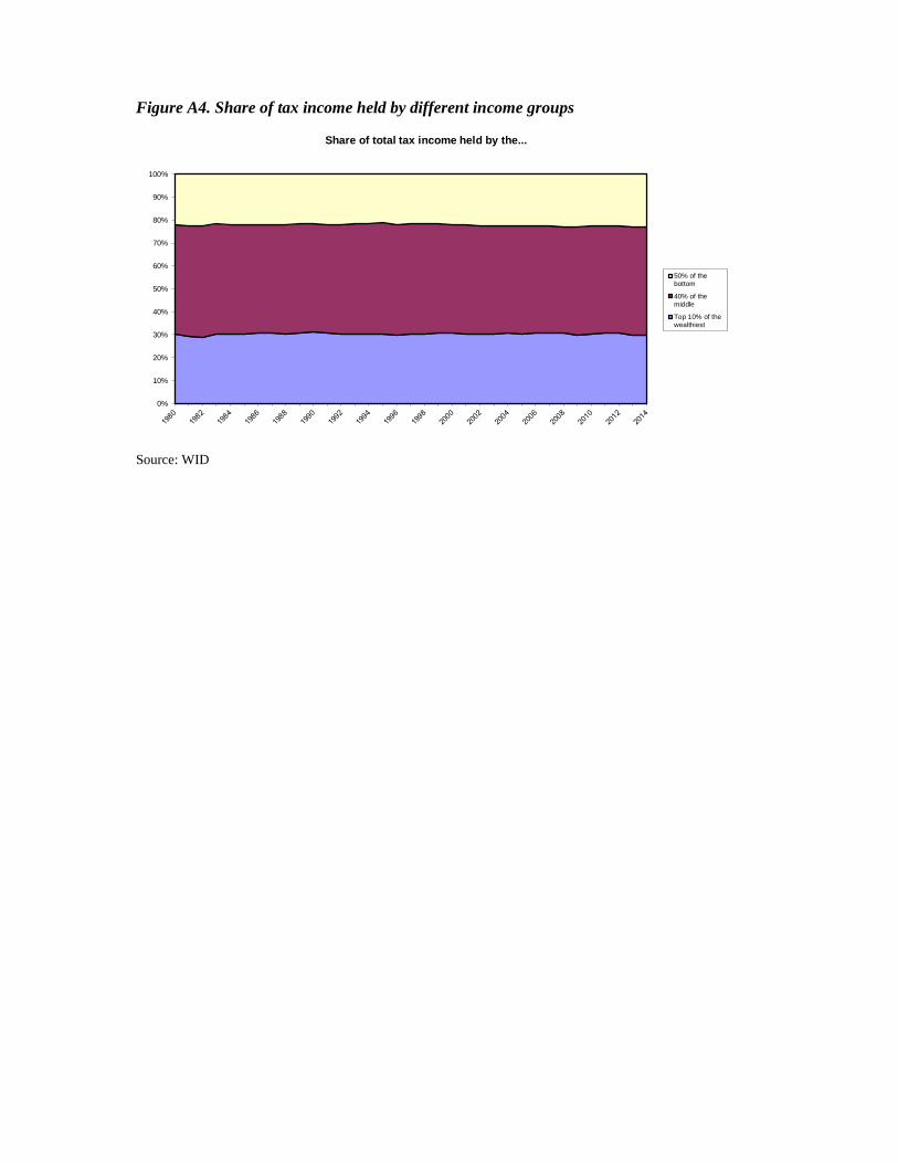
Figure A4. Share of tax income held by different income groups

Source: WID

0%

10%

20%

30%

40%

50%

60%

70%

80%

90%

100%

Share of total tax income held by the...

50% of thebottom

40% of themiddle

Top 10% of thewealthiest

Appendix C. Complementary econometric results

Table A3. First-stage regressions

∆logτi,tIT ∆logτi,t

RSA ∆logτi,tFB

∆logτi,tIT

0.568 ***

(0.003)

0.003

(0.005)

-0.010 **

(0.004)

∆logτi,tRSA

-0.006 ***

(0.001)

0.506 ***

(0.003)

0.002

(0.002)

∆logτi,tFB

0.006 **

(0.002)

-0.001

(0.005)

0.516 ***

(0.003)

∆log ρ̅i,tIT -0.007

(0.026)

0.001

(0.014)

-0.012

(0.011)

∆log ρ̅i,tRSA 0.018

(0.016)

-0.496 ***

(0.027)

0.002

(0.020)

∆log ρ̅i,tFB 0.023 ***

(0.006)

0.069 ***

(0.010)

0.010

(0.007)

Obs 89122 89122 89122

F-stat 574.9 *** 704.0 *** 390.2 *** Note: First stage estimation of equation (9) using all controls.

IT= Income Tax; RSA= In-work benefit; FB= Family Benefit.

Standard errors are in round brackets. Respectively *, *** and *** indicates a significance of 10%, 5% and 1%.

Sample: employees and self-employed people present for two consecutive years, whose labor income represents more than a

quarter of the annual minimum wage.

Source: Insee, ERFS 2006-2015

Table A4. Full results of equation (9) in Table 2

Coefficient Standard

deviation Student T

Constant 9.071 0.036 254.08

𝛽𝜏𝐼𝑇 0.260 0.018 14.63

𝛽𝜏𝑅𝑆𝐴 0.090 0.009 9.74

𝛽𝜏𝑃𝐹 -0.018 0.016 -1.09

𝛽𝜌𝐼𝑇 0.433 0.026 16.61

𝛽𝜌𝑅𝑆𝐴 0.342 0.050 6.78

𝛽𝜌𝑃𝐹 0.065 0.018 3.58

≤19 years old -0.023 0.029 -0.80

20-29 years old 0.031 0.004 8.18

30-39 years old 0.005 0.003 1.68

50-59 years old -0.021 0.003 -7.63

≥60 years old -0.145 0.005 -30.24

Women -0.010 0.002 -4.38

New child since t-1 -0.024 0.003 -6.86

Single parent head of family 0.003 0.005 0.50

Couple without children 0.003 0.003 0.93

Couple with children 0.007 0.003 2.70

"Complex" cleaning -0.000 0.004 -0.01

College (>2 years) 0.070 0.005 13.57

College (≤2 years) 0.065 0.005 13.47

High school graduate 0.050 0.005 10.72

High school diploma or vocational

training 0.033 0.004 7.82

Coefficient Standard

deviation Student T

Constant 9.071 0.036 254.08

𝛽𝜏𝐼𝑇 0.260 0.018 14.63

Lower secondary school or basic

vocational training 0.015 0.005 2.78

Industry 0.055 0.003 17.56

Agriculture 0.012 0.010 1.14

Construction 0.054 0.004 12.06

Part-time worker -0.107 0.003 -35.02

CS 1 -0.050 0.013 -3.77

CS 2 0.003 0.006 0.56

CS 3 0.131 0.004 32.53

CS 4 0.083 0.003 27.79

CS 6 0.039 0.003 12.24

Private permanent contract -0.044 0.003 -16.55

private fixed-term contract -0.039 0.005 -7.25

public CDD 0.001 0.007 0.14

Urban size 1 0.001 0.003 0.42

Urban size 2 0.003 0.003 0.75

Urban size 4 0.004 0.003 1.68

Urban size 5 0.035 0.003 11.09

Occupancy period < 1 year 0.012 0.005 2.47

5-10 years 0.071 0.003 22.70

≥10 years old 0.109 0.003 39.09

Number of employees in the company 0.000 0.000 2.83

2006–2007 0.008 0.005 1.55

2007–2008 0.022 0.005 4.44

2008–2009 -0.014 0.004 -3.24

2009–2010 0.001 0.004 0.27

2010–2011 0.007 0.004 1.81

2011–2012 0.004 0.004 1.10

2012–2013 0.014 0.004 3.60

2014–2014 0.007 0.004 1.88

log(wi,t-1) -1.015 0.004 -234.15

log(wi,t-1) above its 1st decile 0.533 0.012 42.99

log(wi,t-1) above its 2nd decile 0.163 0.026 6.31

log(wi,t-1) above its 3rd decile 0.096 0.050 1.94

log(wi,t-1) above its 4th decile 0.107 0.075 1.43

log(wi,t-1) above its 5th decile -0.054 0.085 -0.63

log(wi,t-1) above its 6th decile -0.009 0.082 -0.11

log(wi,t-1) above its 7th decile -0.032 0.070 -0.46

log(wi,t-1) above its 8th decile 0.156 0.050 3.10

log(wi,t-1) above its 9th decile -0.010 0.025 -0.41

Note: Estimation of equation (9) by 2SLS using A&C instrument, G&S control of the base year income and other controls.

IT= Income tax; PF= Family Benefits; RSA= In-work benefit

Standard errors are in round brackets. Respectively *, *** and *** indicates a significance of 10%, 5% and 1%.

Sample: employees and self-employed people present for two consecutive years, whose labor income represents more than a

quarter of the annual minimum wage.

Source: ERFS 2006-2015

Table A5. Elasticities for different ANTR specifications

(1) Reference

specification

(2) G&S

specification

(3) No ANTR

(3) Participation

rates

𝛽𝜏𝑎𝑙𝑙 0.086 ***

(0.007)

0.085 ***

(0.007)

0.087 ***

(0.007)

0.126 ***

(0.008)

𝛽𝜌𝑎𝑙𝑙 0.255 ***

(0.016)

0.386 ***

(0.024) 0.087 ***

(0.009)

𝛽𝜏𝐼𝑇 0.260 ***

(0.018)

0.267 ***

(0.018)

0.287 ***

(0.018)

0.203 ***

(0.019)

𝛽𝜏𝑅𝑆𝐴 0.090 ***

(0.009)

0.091 ***

(0.009)

0.088 ***

(0.009)

0.074 ***

(0.014)

𝛽𝜏𝐹𝐵 -0.018

(0.016)

-0.018

(0.017)

-0.020

(0.016)

-0.019

(0.016)

𝛽𝜌𝐼𝑇 0.433***

(0.026)

0.556 ***

(0.032)

0.551 ***

(0.015)

𝛽𝜌𝑅𝑆𝐴 0.342 ***

(0.050)

0.562 ***

(0.079)

-0.041

(0.008)

𝛽𝜌𝐹𝐵 0.065 ***

(0.018)

0.096 ***

(0.028)

0.006

(0.036)

Observations 89122 89120 89126 85971 Note: Estimation of equation (9) by 2SLS using A&C instrument, G&S control of the base year income and other controls.

IT= Income Tax; RSA= In-work benefit; FB= Family Benefit; ALL= IT+RSA+ FB;

Standard errors are in round brackets. Respectively *, *** and *** indicates a significance of 10%, 5% and 1%.

Sample: employees and self-employed people present for two consecutive years, whose labor income represents more than a

quarter of the annual minimum wage.

Source: Insee, ERFS 2006-2015

Table A6. Elasticities according to different population restrictions

(1) Reference

specification

(2) Excluding

civil servants

(3) 15 <age <65

years old

𝛽𝜏𝑎𝑙𝑙 0.086 ***

(0.007)

0.087 ***

(0.008)

0.085 ***

(0.007)

𝛽𝜌𝑎𝑙𝑙 0.247 ***

(0.016)

0.270 ***

(0.018)

0.248 ***

(0.016)

𝛽𝜏𝐼𝑇 0.260 ***

(0.018)

0.292 ***

(0.021)

0.263***

(0.018)

𝛽𝜏𝑅𝑆𝐴 0.090 ***

(0.009)

0.086 ***

(0.010)

0.089***

(0.009)

𝛽𝜏𝑃𝐹 -0.018

(0.016)

-0.028

(0.020)

-0.018

(0.016)

𝛽𝜌𝐼𝑇 0.433***

(0.026)

0.469 ***

(0.030)

0.422***

(0.026)

𝛽𝜌𝑅𝑆𝐴 0.342 ***

(0.050)

0.332 ***

(0.055)

0.336***

(0.050)

𝛽𝜌𝑃𝐹 0.065 ***

(0.018)

0.072 ***

(0.021)

0.065***

(0.018)

Observations 89122 71741 88273 Note: Estimation of equation (9) by 2SLS using A&C instrument, G&S control of the base year income and other controls.

IT= Income Tax; RSA= In-work benefit; FB= Family Benefit; ALL= IT+RSA+ FA;

Standard errors are in round brackets. Respectively *, *** and *** indicates a significance of 10%, 5% and 1%.

Sample: employees and self-employed people present for two consecutive years, whose labor income represents more than a quarter

of the annual minimum wage.

Source: Insee, ERFS 2006-2015

Table A7. Elasticities according to weighting

(1) Without weighting

(reference)

(2) With sample weight

(3) Weight=income

𝛽𝜏𝑎𝑙𝑙 0.086 ***

(0.007)

0.080 ***

(0.007)

0.074 ***

(0.008)

𝛽𝜌𝑎𝑙𝑙 0.247 ***

(0.016)

0.250 ***

(0.016)

0.176 ***

(0.014)

𝛽𝜏𝐼𝑇 0.260 ***

(0.018)

0.243 ***

(0.017)

0.170 ***

(0.016)

𝛽𝜏𝑅𝑆𝐴 0.090 ***

(0.009)

0.079 ***

(0.010)

0.097 ***

(0.013)

𝛽𝜏𝑃𝐹 -0.018

(0.016) -0.021 (0.017)

0.004 (0.015)

𝛽𝜌𝐼𝑇 0.433***

(0.026)

0.429 ***

(0.026)

0.204 ***

(0.018)

𝛽𝜌𝑅𝑆𝐴 0.342 ***

(0.050)

0.310 ***

(0.050)

0.279 ***

(0.066)

𝛽𝜌𝑃𝐹 0.065 ***

(0.018)

0.055 ***

(0.019)

0.089 ***

(0.020)

Observations 89122 89120 89120 Note: Estimation of equation (9) by 2SLS using A&C instrument, G&S control of the base year income and other controls.

IT= Income Tax; RSA= In-work benefit; FB= Family Benefit; ALL= IT+RSA+ FA;

Standard errors are in round brackets. Respectively *, *** and *** indicates a significance of 10%, 5% and 1%.

Sample: employees and self-employed people present for two consecutive years, whose labor income represents more than a quarter

of the annual minimum wage.

Source: Insee, ERFS 2006-2015