Embed Size (px)
Citation preview
ReviewSurface Review and Letters, Vol. 8, Nos. 3 & 4 (2001) 367–402c© World Scientific Publishing Company
O Cu(001): I. BINDING THE SIGNATURES OFLEED, STM AND PES IN A BOND-FORMING WAY
CHANG Q. SUN∗
School of Electrical and Electronic Engineering,Nanyang Technological University, Singapore 639798
Received 15 March 2001
This work consists of two sequential parts, which review the advances in uncovering the capacity ofVLEED, STM and PES in revealing the nature and kinetics of oxidation bonding and its consequencesfor the behavior of atoms and valence electrons at a surface; and in quantifying the O–Cu(001) bondingkinetics. The first part describes the model in terms of bond making and its effect on the valence DOSand on the surface potential barrier (SPB) for surfaces with chemisorbed oxygen. One can replace thehydrogen in a H2O molecule with an arbitrary less electronegative element and extend the M2O to asolid surface with Goldschmidt contraction of the bond length, which formulates a specific oxidationsurface with identification of atomic valences and their correspondence to the STM and PES signatures.As consequences of bond making, oxygen derives four additional DOS features in the valence band andabove, i.e. O–M bonding (∼ −5 eV), oxygen nonbonding lone pairs (∼ −2 eV), holes (≤ EF ), andantibonding metal dipoles (≥ EF ), in addition to the hydrogen-bond-like formation. The evolution ofO−1 to O−2 transforms the CuO2 pairing off-centered pyramid in the c(2 × 2)-2O−1 into the Cu3O2
pairing tetrahedron in the (2√
2 ×√
2)R45◦-2O−2 phase on the Cu(001) surface. The new decodingtechnique has enabled the model to be justified and hence the capacity of VLEED, PES and STM tobe fully uncovered in determining simultaneously the bond geometry, the SPB, the valence DOS, andtheir interdependence.
1 Introduction . . . . . . . . . . . . . . . . . . . . . . . . . . . . . . . . . . . . 3681.1 VLEED, STM and PES . . . . . . . . . . . . . . . . . . . . . . . . . . . . . . 3681.2 Known O–Cu(001) identities . . . . . . . . . . . . . . . . . . . . . . . . . . . 3701.3 Objectives . . . . . . . . . . . . . . . . . . . . . . . . . . . . . . . . . . . . 373
2 Theory Models . . . . . . . . . . . . . . . . . . . . . . . . . . . . . . . . . . . 3732.1 VLEED multiatom code . . . . . . . . . . . . . . . . . . . . . . . . . . . . . . 3732.2 Chemical bond . . . . . . . . . . . . . . . . . . . . . . . . . . . . . . . . . . 3742.3 Valence density-of-state (DOS) . . . . . . . . . . . . . . . . . . . . . . . . . . . 3832.4 3D surface potential barrier (SPB) . . . . . . . . . . . . . . . . . . . . . . . . . 384
3 VLEED Numerical Justification . . . . . . . . . . . . . . . . . . . . . . . . . . . 3913.1 Decoding methodology . . . . . . . . . . . . . . . . . . . . . . . . . . . . . . . 3913.2 Code validity . . . . . . . . . . . . . . . . . . . . . . . . . . . . . . . . . . . 3933.3 Model confirmation . . . . . . . . . . . . . . . . . . . . . . . . . . . . . . . . 397
4 Summary . . . . . . . . . . . . . . . . . . . . . . . . . . . . . . . . . . . . . . 400Acknowledgments . . . . . . . . . . . . . . . . . . . . . . . . . . . . . . . . . . . 400References . . . . . . . . . . . . . . . . . . . . . . . . . . . . . . . . . . . . . . . 401
∗Fax: 65 6792 0415. E-mail: [email protected]
367
368 C. Q. Sun
1. Introduction
The text of this article, Part I, is arranged as follows.
Section 1 gives a brief survey of the knowledge ac-
quired so far about O–Cu(001) surface reaction and
the objectives of this exercise. Section 2 describes
the model for the oxide tetrahedron bonding and its
consequence on the valence DOS and the surface po-
tential barrier (SPB) in general, in addition to the
specific O–Cu(001) surface. Qualitative information
is gained about the change of the bond geometry, va-
lence DOS and SPB by incorporating the model with
STM and PES observations. Section 3 demonstrates
the numerical justifications for the models, the de-
coding skills and the VLEED code that was devel-
oped by Thurgate1 based on the LEED package of
Van Hove and Tong.2 It is shown that VLEED can be
used to simultaneously determine the bond geometry
and the behavior of valence electrons both in real and
in energy spaces. In Part II,3 I will show the reliabil-
ity of the VLEED technique, the solution certainty
and the outcomes of decoding a series of dynamic
VLEED I–E spectra from the O–Cu(001) surface. It
is striking that the reaction can be decoded as four
discrete stages of bond-forming kinetics.
1.1. VLEED, STM and PES
Unlike the normal LEED, in which the scattering
is dominated by interaction between the incident
electron beams and the ion cores of a number of
stacking layers of atoms,2,4 LEED at very low en-
ergies (VLEED) below plasma excitation (∼ 15 eV
below EF ) reveals rich and profound information
about not only the crystal geometry of the topmost
atomic layers but also the behavior of surface elec-
trons. The conjunction of the SPB with the multiple
scattering gives rise to the interesting phenomena of
surface states, surface resonance and VLEED fine
structures.5,6 The fine-structure features in VLEED
I–E spectra are determined by the interaction be-
tween the incident beams and the surface electrons
that are linked closely to the positions and valences
of the atoms at the surface. The VLEED spectrum
integrates the following information:1 (i) diffraction
from the ion cores of a very few surface atomic layers
depending on the beam energy; (ii) scattering and
interference by the elastic SPB; and (iii) attenua-
tion by the inelastic SPB, or exchanging energy with
surface electrons and excitation of phonons and pho-
tons. Therefore, the mechanism for VLEED is much
more complicated than that for the normal LEED.
Because of the difficulties arising from the ef-
fects of stray electronic and magnetic fields on slowly
moving electrons, the VLEED technique is not often
used.1 Also, theory calculations usually do not ex-
tend to these low energies because of the approxima-
tion in the calculation code. These include the use of
an optical potential independent of electron energy,
which is valid at higher energies but becomes unre-
liable at energies below the plasmon-excitation ener-
gies. Furthermore, the spectra contain fine struc-
tures that are sensitive to the shape of the SPB.
These features do not arise in conventional LEED
calculations, where SPB scattering is treated in a
simple fashion. It seemed impossible to use VLEED
to simultaneously determine the crystal geometry
and the SPB, as one was unable to identify the spec-
tral feature arising from the change of either atomic
positions or the shape of the SPB. In circumstances
where the shape of the SPB, the energy dependence
of the inner potential and the spatial decay and en-
ergy dependence of the imaginary potential are un-
known, it would be imprudent to attempt to derive
too much independent structural information from
the VLEED fine-structure features alone.7 Appro-
priate modeling which includes all the contributions
aforementioned and their naturely interdependence
in decoding the VLEED data is therefore necessary.
On the other hand, VLEED possesses more ad-
vantages than LEED in obtaining information about
the SPB and the energy band structure, as demon-
strated for several mostly close-packed surfaces of
transition metals.8–14 The scattering of VLEED
beams from light adsorbates is often stronger, even
comparable to the substrate host atoms, and this
can lead to improved knowledge of the adsorbates
positions15 as well as the valences of individual sur-
face atoms with the assistance of an appropriate
model. This is due to bond formation that modi-
fies the electronic structures of the negative ions of
the light adsorbates and alters the valences of the
host atoms. Moreover, in VLEED calculations, fewer
beams and fewer phase shifts are considered and
spectral peaks occur with a greater density. Hence,
computation time is considerably reduced. Fur-
nished with an appropriate calculation code and suit-
able models, the high-resolution VLEED data can be
O–Cu(001): I. Binding the Signatures of LEED, STM and PES in a Bond-Forming Way 369
analyzed for comprehensive information about the
behavior of atoms and electrons at a surface.
There are two kinds of characteristic features on a
measured VLEED spectrum. One is the Rydberg se-
ries that relate to the interference or resonance effect
due to the SPB,16 and the other sharp features come
from the band gap.10 The Rydberg features come
from the interference between the measured beam
and the pre-emergent beams that reflect repeat-
edly between the substrate lattice and the SPB.6,17
The Rydberg series are often known as “threshold
effects” or “SPB resonance or interference,”18 since
they converge from below the emergence thresholds
of diffracted beams. The positions of the narrow,
sharp, solitary and violent peaks rely both on the
crystal geometry of the surface and on the incident
and azimuth angles of the electron beams.19,20 The
sharp peaks converge into the thresholds of emerg-
ing new beams inside the crystal, as found from
the O–Ru(0001),21 Cu(111) and Ni(111)12 and the
ZnO(0001)11 surfaces. These features are suggested
as being issued from the energy-band structure. The
troughs relate to the intensity variation caused by
the wavelike energy dependence of the additional
sextets in the VLEED pattern.22 The relationship
between the band structure and the elastic reflec-
tion coefficient can be obtained through the match-
ing method.10,23 In this approach, the elastic reflec-
tion coefficient is determined by matching the vac-
uum wave function with the superposition of Bloch
waves excited in the solid. It is expected24,25 that the
energy of a trough in the spectrum, corresponding to
the rapid change of reflection, coincides with the lo-
cation of the band-structure critical positions at the
boundaries of Brillouin zones. Therefore, it is possi-
ble, as noted by Jacklevic and Davis,10 to determine
the connection between the VLEED profiles and the
band structure by directly measuring the positions
of the critical points. Many researchers have also de-
voted their efforts to using VLEED to characterize
the energy states above the vacuum level of the sur-
faces. Strocov et al.12,13 demonstrated that VLEED
measurements are ideally suited for accurate deter-
mination of the desired upper states. Knowledge of
the excited states could be substantially more im-
proved than could the band mapping by PES. From
the band-structure point of view, this indicates sen-
sitivity of VLEED to the modifications of the upper
band structure formed by the variations of geomet-
ric structure and encourages one to use VLEED as
a tool for investigating which way these two entities,
i.e. atomic geometry and band structures, are inter-
dependent. Furthermore, Bartos et al.26 found that
corresponding theoretical VLEED I–E curves could
be obtained in good agreement with experimental
data from the Cu(111) surface when the anisotropy
of the electron attenuation (inelastic potential) was
taken into account. Therefore, VLEED also gives
information about the anisotropy of the SPB.
Unfortunately, little progress had been made un-
til 1995 in the structure determination of surfaces
with large unit meshes or surfaces with adsorbed
molecules using VLEED. No attempts had even been
made using VLEED to simultaneously determine the
bond geometry, energy states, the three-dimensional
(3D) SPB and the bond-forming kinetics of systems
with chemisorbed oxygen. The situation changed
when a calculation code was developed, which made
it possible to deal with the O-adsorbed system. In
the new code, a complex unit cell composed of five
atoms was employed, and the SPB was treated as an
additional uniform layer of interference added to the
system of multiple scattering. However, the param-
eter space used to describe the elastic ReV (z) and
the inelastic ImV (z, E) part of the SPB was still too
large. At least nine variables in a one-dimensional
(1D) system were required to describe the spatial
variation and energy dependence of the SPB. In-
formation, such as valences, the nonuniformity and
anisotropy of the SPB, was missed with the 1D-SPB
approximation in which the strongly correlated pa-
rameters were treated independently. Such a wisdom
worked well for the Cu(001) clean surface but faced
difficulties in decoding the VLEED data from the
O–Cu(001) surface. Spectra near the 〈11〉 azimuth
of the O–Cu(001) surface could not be fitted despite
various structure models and SPB parameters having
been tried.1 The 3D effects in the SPB are likely to
be crucial for the adsorbate-involved system,27 which
is rather local on an atomic scale in many properties.
Furthermore, as suggested by Pfnur et al.,15 correct
SPB parameters must depend on energy E, lateral
momentum K‖ and surface coordinates (x, y). How-
ever, the primary effect of the 3D terms in the SPB is
to generate off-diagonal matrix elements in the SPB
scattering matrix, which leads to too much longer
computer running. One way to include the 3D effects
in a simpler manner is to use a hybridized 1D SPB
370 C. Q. Sun
model that incorporates some of the more important
3D effects. Fortunately it is believed15 that multi-
ple scattering is often less important in the VLEED
energies, so the hybridization of the 1D SPB model
with 3D contribution is acceptable.
When the high-energy photons, X-rays or ultra-
violet rays slam into the sample, they evict some
of its electrons, launching them out of the material.
Detectors then count these homeless electrons and
measure their energy and direction of travel. UPS,
which examines electrons ejected from valence shells,
is more suited to establishing the bonding character-
istics and the details of valence-shell electronic struc-
tures of substances on the surface. Its usefulness is
its ability to reveal which orbitals of the adsorbate
are involved in the bond to the substrate host. At
low energies the unoccupied states have structures.
Consequently, if photoelectrons ejected from filled
levels have kinetic energies (KE’s) that fall within
this structured region, the observed intensity will be
a convolution of the filled and empty DOS together
with the matrix of transition probabilities. This is
the case in UPS that gives rise to the strong depen-
dence of valence-level spectra on photon energy. In
the case of XPS the KE of the valence photoelec-
trons is such that the final states are quite devoid of
structure; thus the observed DOS closely reflects the
initial filled DOS. The complete spectrum at high
resolution shows the band structure and the sharp
cutoff in electron density at EF .
The invention of STM has led to enormous
progress in revealing direct and qualitative in-
formation on an atomic scale about the surface
but the images challenge suitable physical inter-
pretation.28 VLEED, PES and STM can be used as
complementary tools to get such information that in-
tegrates both real space and k space, on an atomic
scale and over macroscopic areas of the surface.
Combination of VLEED with STM, STS and PES
certainly reduces the limitations inherent in each of
these techniques used separately. STM observation
provides us with a direct vision of the surface mor-
phology; decoding VLEED spectra rewards us with
the quantitative details. Based on a certain num-
ber of physical premises and STM imaging, one may
be able to formulate a specific system to specify the
individual atomic valence and elucidate the driving
force as well as the corresponding SPB. Derivations
of these models from STM images can be used as
input and also justification in simulating VLEED
spectra. The simulation results, in turn, improve
the understanding of the STS and PES profiles and
STM images. Thus one can extract comprehensive
and quantitative information from such a combina-
tion about the behavior of atoms and electrons at
surfaces. If one could specify the STM signatures
come from whether ionic, polarized, or vacancy of
missed atoms, then the elucidation of information
from the identities would be much easier.29
1.2. Known O Cu(001) identities
As one of the prototypes of catalytic oxidation,
the O–Cu(001) surface has been intensively inves-
tigated. Since 1956, when Young et al.30 found
that the Cu(001) surface is easier to be oxidized
than other planes of the copper single crystal, there
have been many conflicting opinions regarding the
oxygen-induced reconstruction of the Cu(001) sur-
face. Different atomic superstructures have been
derived with various experimental techniques31 and
theoretical approaches.32,33 It is very interesting that
the observed structures vary considerably from re-
searcher to researcher even though they used the
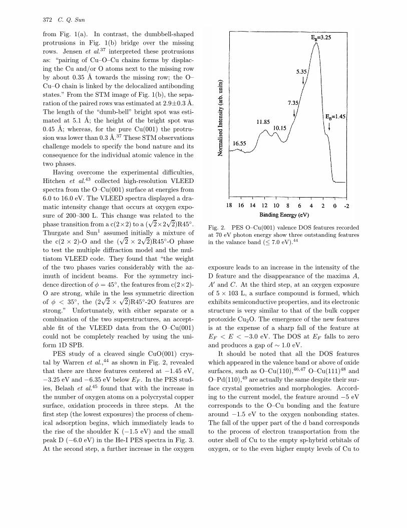
same approach. The missing-row (MR) type (√
2 ×2√
2)R45◦-2O reconstruction first proposed by Zeng
and Mitchell in 1988 has been elegantly accepted.34
The latest conclusion35,36 was that an off-centered
pyramid, or less ordered c(2 × 2)-O, forms first
at oxygen exposure lower than 25 L, and then
the (√
2× 2√
2)R45◦-2O MR superstructure follows.
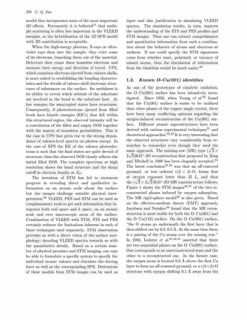
Figure 1 shows the STM images36,37 of the two re-
constructed phases induced by oxygen adsorption.
The MR rigid-sphere model38 is also given. Based
on the effective-medium theory (EMT) approach,
Jacobsen and Nørskov39 found that the MR recon-
struction is most stable for both the O–Cu(001) and
the O–Cu(110) surface. On the O–Cu(001) surface,
“the O atoms go underneath the first layer that is
then shifted out by 0.3–0.5 A. At the same time there
is a pairing of the Cu atoms over the missing row.”
In 1993, Lederer et al.35,40,41 asserted that there
are two sequential phases on the O–Cu(001) surface.
One corresponds to an unreconstructed state and the
other to a reconstructed one. In the former case,
the oxygen atom is located 0.8 A above the first Cu
layer to form an off-centered pyramid, or a c(2×2)-O
structure with oxygen shifting 0.1 A away from the
O–Cu(001): I. Binding the Signatures of LEED, STM and PES in a Bond-Forming Way 371
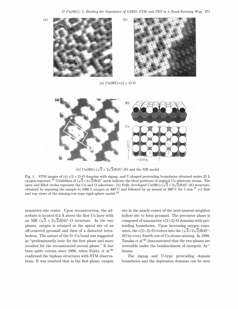
(a) (b)
(a) Cu(001)-c(2× 2)-O
���
(b) Cu(001)-(√
2× 2√
2)R45◦-2O and the MR model
Fig. 1. STM images of (a) c(2× 2)-O domains with zigzag- and U-shaped protruding boundaries obtained under 25 Loxygen exposure.36 Guidelines of (
√2×2√
2)R45◦ mesh indicate the ideal positions of original Cu substrate atoms. Theopen and filled circles represent the Cu and O adsorbate. (b) Fully developed Cu(001)-(
√2× 2
√2)R45◦-2O structure,
obtained by exposing the sample to 1000 L oxygen at 300◦C and followed by an anneal at 300◦C for 5 min.37 (c) Sideand top views of the missing-row-type rigid-sphere model.38
symmetry-site center. Upon reconstruction, the ad-
sorbate is located 0.2 A above the first Cu layer with
an MR (√
2 × 2√
2)R45◦-O structure. In the two
phases, oxygen is retained at the apical site of an
off-centered pyramid and then of a distorted tetra-
hedron. The nature of the O–Cu bond was suggested
as “predominantly ionic for the first phase and more
covalent for the reconstructed second phase.” It has
been quite certain since 1996, when Fujita et al.36
confirmed the biphase structures with STM observa-
tions. It was resolved that in the first phase, oxygen
sits in the nearly-center of the next-nearest-neighbor
hollow site to form pyramid. The precursor phase is
composed of nanometric c(2×2)-O domains with pro-
truding boundaries. Upon increasing oxygen expo-
sures, the c(2×2)-O evolves into the (√
2×2√
2)R45◦-
2O by every fourth row of Cu atoms missing. In 1998,
Tanaka et al.42 demonstrated that the two phases are
reversible under the bombardment of energetic Ar+
beams.
The zigzag and U-type protruding domain
boundaries and the depression domains can be seen
372 C. Q. Sun
from Fig. 1(a). In contrast, the dumbbell-shaped
protrusions in Fig. 1(b) bridge over the missing
rows. Jensen et al.37 interpreted these protrusions
as: “pairing of Cu–O–Cu chains forms by displac-
ing the Cu and/or O atoms next to the missing row
by about 0.35 A towards the missing row; the O–
Cu–O chain is linked by the delocalized antibonding
states.” From the STM image of Fig. 1(b), the sepa-
ration of the paired rows was estimated at 2.9±0.3 A.
The length of the “dumb-bell” bright spot was esti-
mated at 5.1 A; the height of the bright spot was
0.45 A; whereas, for the pure Cu(001) the protru-
sion was lower than 0.3 A.37 These STM observations
challenge models to specify the bond nature and its
consequence for the individual atomic valence in the
two phases.
Having overcome the experimental difficulties,
Hitchen et al.43 collected high-resolution VLEED
spectra from the O–Cu(001) surface at energies from
6.0 to 16.0 eV. The VLEED spectra displayed a dra-
matic intensity change that occurs at oxygen expo-
sure of 200–300 L. This change was related to the
phase transition from a c(2×2) to a (√
2×2√
2)R45◦.
Thurgate and Sun1 assumed initially a mixture of
the c(2 × 2)-O and the (√
2 × 2√
2)R45◦-O phase
to test the multiple diffraction model and the mul-
tiatom VLEED code. They found that “the weight
of the two phases varies considerably with the az-
imuth of incident beams. For the symmetry inci-
dence direction of φ = 45◦, the features from c(2×2)-
O are strong, while in the less symmetric direction
of φ < 35◦, the (2√
2 ×√
2)R45◦-2O features are
strong.” Unfortunately, with either separate or a
combination of the two superstructures, an accept-
able fit of the VLEED data from the O–Cu(001)
could not be completely reached by using the uni-
form 1D SPB.
PES study of a cleaved single CuO(001) crys-
tal by Warren et al.,44 as shown in Fig. 2, revealed
that there are three features centered at −1.45 eV,
−3.25 eV and −6.35 eV below EF . In the PES stud-
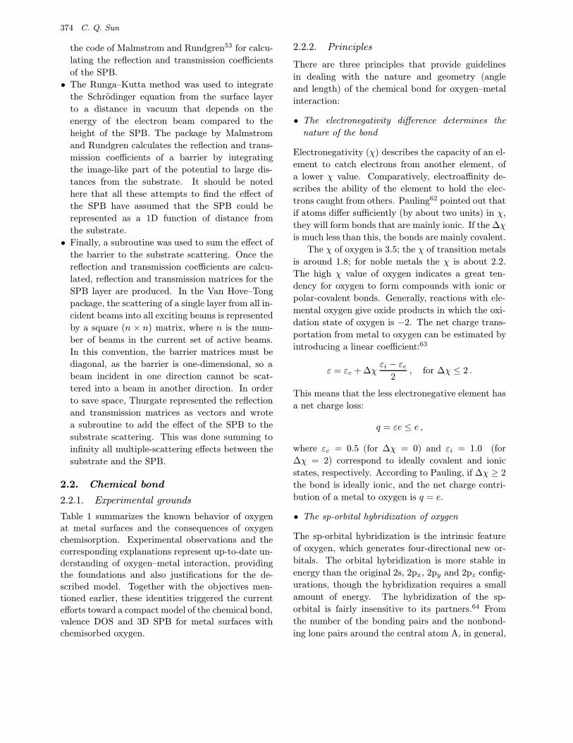
ies, Belash et al.45 found that with the increase in
the number of oxygen atoms on a polycrystal copper
surface, oxidation proceeds in three steps. At the
first step (the lowest exposures) the process of chem-
ical adsorption begins, which immediately leads to
the rise of the shoulder K (−1.5 eV) and the small
peak D (−6.0 eV) in the He-I PES spectra in Fig. 3.
At the second step, a further increase in the oxygen
Fig. 2. PES O–Cu(001) valence DOS features recordedat 70 eV photon energy show three outstanding featuresin the valance band (≤ 7.0 eV).44
exposure leads to an increase in the intensity of the
D feature and the disappearance of the maxima A,
A′ and C. At the third step, at an oxygen exposure
of 5 × 10³ L, a surface compound is formed, which
exhibits semiconductive properties, and its electronic
structure is very similar to that of the bulk copper
protoxide Cu2O. The emergence of the new features
is at the expense of a sharp fall of the feature at
EF < E < −3.0 eV. The DOS at EF falls to zero
and produces a gap of ∼ 1.0 eV.
It should be noted that all the DOS features
which appeared in the valence band or above of oxide
surfaces, such as O–Cu(110),46,47 O–Cu(111)48 and
O–Pd(110),49 are actually the same despite their sur-
face crystal geometries and morphologies. Accord-
ing to the current model, the feature around −5 eV
corresponds to the O–Cu bonding and the feature
around −1.5 eV to the oxygen nonbonding states.
The fall of the upper part of the d band corresponds
to the process of electron transportation from the
outer shell of Cu to the empty sp-hybrid orbitals of
oxygen, or to the even higher empty levels of Cu to
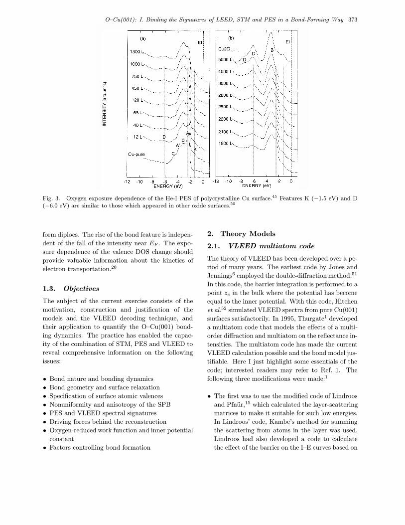
O–Cu(001): I. Binding the Signatures of LEED, STM and PES in a Bond-Forming Way 373
Fig. 3. Oxygen exposure dependence of the He-I PES of polycrystalline Cu surface.45 Features K (−1.5 eV) and D(−6.0 eV) are similar to those which appeared in other oxide surfaces.50
form diploes. The rise of the bond feature is indepen-
dent of the fall of the intensity near EF . The expo-
sure dependence of the valence DOS change should
provide valuable information about the kinetics of
electron transportation.20
1.3. Objectives
The subject of the current exercise consists of the
motivation, construction and justification of the
models and the VLEED decoding technique, and
their application to quantify the O–Cu(001) bond-
ing dynamics. The practice has enabled the capac-
ity of the combination of STM, PES and VLEED to
reveal comprehensive information on the following
issues:
• Bond nature and bonding dynamics
• Bond geometry and surface relaxation
• Specification of surface atomic valences
• Nonuniformity and anisotropy of the SPB
• PES and VLEED spectral signatures
• Driving forces behind the reconstruction
• Oxygen-reduced work function and inner potential
constant
• Factors controlling bond formation
2. Theory Models
2.1. VLEED multiatom code
The theory of VLEED has been developed over a pe-
riod of many years. The earliest code by Jones and
Jennings6 employed the double-diffraction method.51
In this code, the barrier integration is performed to a
point zc in the bulk where the potential has become
equal to the inner potential. With this code, Hitchen
et al.52 simulated VLEED spectra from pure Cu(001)
surfaces satisfactorily. In 1995, Thurgate1 developed
a multiatom code that models the effects of a multi-
order diffraction and multiatom on the reflectance in-
tensities. The multiatom code has made the current
VLEED calculation possible and the bond model jus-
tifiable. Here I just highlight some essentials of the
code; interested readers may refer to Ref. 1. The
following three modifications were made:1
• The first was to use the modified code of Lindroos
and Pfnur,15 which calculated the layer-scattering
matrices to make it suitable for such low energies.
In Lindroos’ code, Kambe’s method for summing
the scattering from atoms in the layer was used.
Lindroos had also developed a code to calculate
the effect of the barrier on the I–E curves based on
374 C. Q. Sun
the code of Malmstrom and Rundgren53 for calcu-
lating the reflection and transmission coefficients
of the SPB.
• The Runga–Kutta method was used to integrate
the Schrodinger equation from the surface layer
to a distance in vacuum that depends on the
energy of the electron beam compared to the
height of the SPB. The package by Malmstrom
and Rundgren calculates the reflection and trans-
mission coefficients of a barrier by integrating
the image-like part of the potential to large dis-
tances from the substrate. It should be noted
here that all these attempts to find the effect of
the SPB have assumed that the SPB could be
represented as a 1D function of distance from
the substrate.
• Finally, a subroutine was used to sum the effect of
the barrier to the substrate scattering. Once the
reflection and transmission coefficients are calcu-
lated, reflection and transmission matrices for the
SPB layer are produced. In the Van Hove–Tong
package, the scattering of a single layer from all in-
cident beams into all exciting beams is represented
by a square (n × n) matrix, where n is the num-
ber of beams in the current set of active beams.
In this convention, the barrier matrices must be
diagonal, as the barrier is one-dimensional, so a
beam incident in one direction cannot be scat-
tered into a beam in another direction. In order
to save space, Thurgate represented the reflection
and transmission matrices as vectors and wrote
a subroutine to add the effect of the SPB to the
substrate scattering. This was done summing to
infinity all multiple-scattering effects between the
substrate and the SPB.
2.2. Chemical bond
2.2.1. Experimental grounds
Table 1 summarizes the known behavior of oxygenat metal surfaces and the consequences of oxygenchemisorption. Experimental observations and thecorresponding explanations represent up-to-date un-derstanding of oxygen–metal interaction, providingthe foundations and also justifications for the de-scribed model. Together with the objectives men-tioned earlier, these identities triggered the currentefforts toward a compact model of the chemical bond,valence DOS and 3D SPB for metal surfaces withchemisorbed oxygen.
2.2.2. Principles
There are three principles that provide guidelines
in dealing with the nature and geometry (angle
and length) of the chemical bond for oxygen–metal
interaction:
• The electronegativity difference determines the
nature of the bond
Electronegativity (χ) describes the capacity of an el-
ement to catch electrons from another element, of
a lower χ value. Comparatively, electroaffinity de-
scribes the ability of the element to hold the elec-
trons caught from others. Pauling62 pointed out that
if atoms differ sufficiently (by about two units) in χ,
they will form bonds that are mainly ionic. If the ∆χ
is much less than this, the bonds are mainly covalent.
The χ of oxygen is 3.5; the χ of transition metals
is around 1.8; for noble metals the χ is about 2.2.
The high χ value of oxygen indicates a great ten-
dency for oxygen to form compounds with ionic or
polar-covalent bonds. Generally, reactions with ele-
mental oxygen give oxide products in which the oxi-
dation state of oxygen is −2. The net charge trans-
portation from metal to oxygen can be estimated by
introducing a linear coefficient:63
ε = εc + ∆χεi − εc
2, for ∆χ ≤ 2 .
This means that the less electronegative element has
a net charge loss:
q = εe ≤ e ,
where εc = 0.5 (for ∆χ = 0) and εi = 1.0 (for
∆χ = 2) correspond to ideally covalent and ionic
states, respectively. According to Pauling, if ∆χ ≥ 2
the bond is ideally ionic, and the net charge contri-
bution of a metal to oxygen is q = e.
• The sp-orbital hybridization of oxygen
The sp-orbital hybridization is the intrinsic feature
of oxygen, which generates four-directional new or-
bitals. The orbital hybridization is more stable in
energy than the original 2s, 2px, 2py and 2pz config-
urations, though the hybridization requires a small
amount of energy. The hybridization of the sp-
orbital is fairly insensitive to its partners.64 From
the number of the bonding pairs and the nonbond-
ing lone pairs around the central atom A, in general,
O–Cu(001): I. Binding the Signatures of LEED, STM and PES in a Bond-Forming Way 375
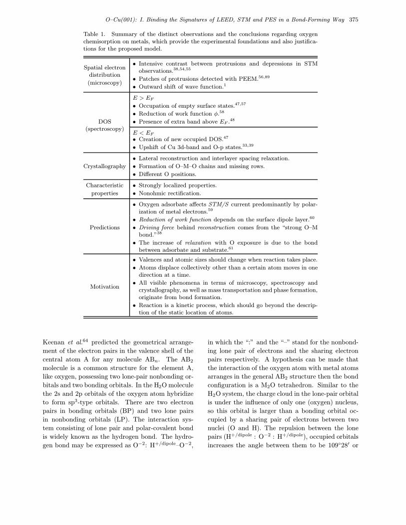
Table 1. Summary of the distinct observations and the conclusions regarding oxygenchemisorption on metals, which provide the experimental foundations and also justifica-tions for the proposed model.
Spatial electron• Intensive contrast between protrusions and depressions in STM
observations.38,54,55
distribution • Patches of protrusions detected with PEEM.56,89
(microscopy) • Outward shift of wave function.1
E > EF
• Occupation of empty surface states.47,57
• Reduction of work function φ.58
DOS • Presence of extra band above EF .48
(spectroscopy)E < EF• Creation of new occupied DOS.47
• Upshift of Cu 3d-band and O-p states.33,39
• Lateral reconstruction and interlayer spacing relaxation.
Crystallography • Formation of O–M–O chains and missing rows.
• Different O positions.
Characteristic • Strongly localized properties.
properties • Nonohmic rectification.
• Oxygen adsorbate affects STM/S current predominantly by polar-ization of metal electrons.59
• Reduction of work function depends on the surface dipole layer.60
Predictions • Driving force behind reconstruction comes from the “strong O–Mbond.”38
• The increase of relaxation with O exposure is due to the bondbetween adsorbate and substrate.61
• Valences and atomic sizes should change when reaction takes place.
• Atoms displace collectively other than a certain atom moves in onedirection at a time.
Motivation• All visible phenomena in terms of microscopy, spectroscopy and
crystallography, as well as mass transportation and phase formation,originate from bond formation.
• Reaction is a kinetic process, which should go beyond the descrip-tion of the static location of atoms.
Keenan et al.64 predicted the geometrical arrange-
ment of the electron pairs in the valence shell of the
central atom A for any molecule ABn. The AB2
molecule is a common structure for the element A,
like oxygen, possessing two lone-pair nonbonding or-
bitals and two bonding orbitals. In the H2O molecule
the 2s and 2p orbitals of the oxygen atom hybridize
to form sp3-type orbitals. There are two electron
pairs in bonding orbitals (BP) and two lone pairs
in nonbonding orbitals (LP). The interaction sys-
tem consisting of lone pair and polar-covalent bond
is widely known as the hydrogen bond. The hydro-
gen bond may be expressed as O−2: H+/dipole–O−2,
in which the “:” and the “–” stand for the nonbond-
ing lone pair of electrons and the sharing electron
pairs respectively. A hypothesis can be made that
the interaction of the oxygen atom with metal atoms
arranges in the general AB2 structure then the bond
configuration is a M2O tetrahedron. Similar to the
H2O system, the charge cloud in the lone-pair orbital
is under the influence of only one (oxygen) nucleus,
so this orbital is larger than a bonding orbital oc-
cupied by a sharing pair of electrons between two
nuclei (O and H). The repulsion between the lone
pairs (H+/dipole : O−2 : H+/dipole), occupied orbitals
increases the angle between them to be 109◦28′ or
376 C. Q. Sun
more. Meanwhile, their repulsions toward the elec-
tron pairs in the bonding orbitals push the bonding
orbitals (H+/dipole–O−2–H+/dipole) closer together,
thereby reducing the H+/dipole–O−2–H+/dipole bond
angle from the tetrahedral value to 104.5◦ or less.
The order of repulsion energies is LP–LP > LP–BP
> BP–BP.
• The atomic radius contracts with the reduction
of CN
In reality, surface reaction results in charge transfer
between oxygen and metal atoms. Atomic radii are
no longer constant when atoms alter their valences
from metallic to either ionic or polarized. For in-
stance, the radius of Cu reduces from 1.27 to 0.53 A
when the Cu becomes Cu+ while the radius of O in-
creases from 0.64 to 1.32 A when O turns into O−2.
It should be emphasized that atoms are not hard
spheres of constant size; rather, the atomic radius
changes with the coordination. In a way this is to be
expected, since an atom shared 6 ways would have a
radius different from that of the same atom shared
12 ways. As the CN decreases, the atomic radius
decreases. Goldschmidt65 classified that if a CN of
12 as a standard changes to 8, 6 and 4, there is re-
spectively a 3%, 4% and 12% shrinking in the ionic
radius. EMT calculations38 also revealed the ten-
dency of the O–Cu bond length to decrease with CN.
Pauling66 found relations between CN and metallic
radius. This theory contains numerous assumptions
and is somewhat empirical in nature. However, it
does give some surprisingly good answers in certain
cases.67 According to Pauling, the Cu radius will
change from 1.276 to 1.173 A (about 8% contraction)
if the CN changes from 12 to 1 (only one neighbor).
Jorgensen68 and Kamimura et al.69 noticed that the
Cu-apical oxygen (at the apex of the octagonal CuO6
structure) bond length is shortened with the increase
of dopant-hole concentration. The reduction of the
O–Cu distance is as high as 0.26 A (about 14% con-
traction) in La–Sr–Cu–O superconducting materials.
Hence, besides the atomic-radius alternation due to
the change of valence state, the reduced CN of the
surface atoms results in a further reduction of the
atomic radii of these atoms, which is independent of
the bond nature.67 Goldschmidt’s contraction of the
ionic radius can be defined by
R(CN) = R(12)× [1−Q(CN)] ,
�
�
��
�
�
��
������������
������������
� ��� ������
� ��������� ������
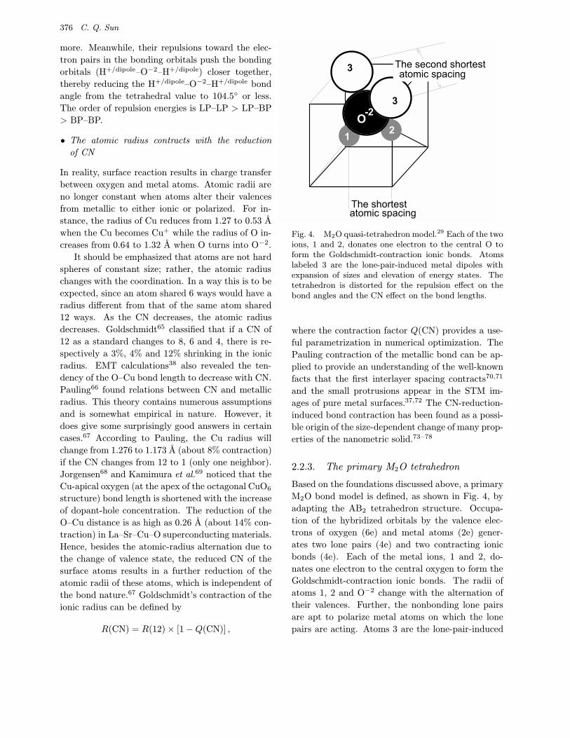
Fig. 4. M2O quasi-tetrahedron model.29 Each of the twoions, 1 and 2, donates one electron to the central O toform the Goldschmidt-contraction ionic bonds. Atomslabeled 3 are the lone-pair-induced metal dipoles withexpansion of sizes and elevation of energy states. Thetetrahedron is distorted for the repulsion effect on thebond angles and the CN effect on the bond lengths.
where the contraction factor Q(CN) provides a use-
ful parametrization in numerical optimization. The
Pauling contraction of the metallic bond can be ap-
plied to provide an understanding of the well-known
facts that the first interlayer spacing contracts70,71
and the small protrusions appear in the STM im-
ages of pure metal surfaces.37,72 The CN-reduction-
induced bond contraction has been found as a possi-
ble origin of the size-dependent change of many prop-
erties of the nanometric solid.73–78
2.2.3. The primary M2O tetrahedron
Based on the foundations discussed above, a primary
M2O bond model is defined, as shown in Fig. 4, by
adapting the AB2 tetrahedron structure. Occupa-
tion of the hybridized orbitals by the valence elec-
trons of oxygen (6e) and metal atoms (2e) gener-
ates two lone pairs (4e) and two contracting ionic
bonds (4e). Each of the metal ions, 1 and 2, do-
nates one electron to the central oxygen to form the
Goldschmidt-contraction ionic bonds. The radii of
atoms 1, 2 and O−2 change with the alternation of
their valences. Further, the nonbonding lone pairs
are apt to polarize metal atoms on which the lone
pairs are acting. Atoms 3 are the lone-pair-induced
O–Cu(001): I. Binding the Signatures of LEED, STM and PES in a Bond-Forming Way 377
metal dipoles with expansion of dimension and el-
evation of energy states, which are presumably re-
sponsible for the protrusions in the STM images and
the reduction of the local work function. This event
agrees with Lang’s tunneling theory79 which predicts
that the oxygen adsorbate affects the tunnel current
predominantly by polarization of metal electrons.
The primary M2O tetrahedron is distorted for
two effects: (i) the repulsion difference varies the
bond angles [BAij (∠iOj), i, j = 1, 2, 3; BA12 ≤104.5◦, BA33 > 109.5◦], and (ii) the CN reduction
adjusts the individual bond length [BLi = (RM+ +
RO−2) × (1 − Qi), i = 1, 2; Qi is the effective
contracting factors]. BL3 and BA33 vary with the
coordination circumstances in a real system.
The coordination surroundings of a specific
system, i.e. the crystal geometry and the scale of
the lattice constant facilitate the tetrahedron. The
ideal coordination environment is that, as denoted
in the diagram, the distances of 1–2 and 3–3 match
closely the first and the second shortest atomic spac-
ings. The plane composed of 1O2 is perpendicular to
the plane of 3O3. In reality, atomic dislocation is not
avoidable for the bond formation. Moreover, oxygen
always seeks four neighbors to form a stable tetrahe-
dron. It should be noted that the lone-pair-induced
dipoles tend to be directed to the open end of a sur-
face due to the strong repulsion between lone pairs
and between the lone-pair-induced dipoles. There-
fore, atomic dislocations during the reaction are
determined by the bond geometry.
With the adaptation of the general AB2 molecule
to the M2O system, the M2O system contains three
valences, namely the O−2-hybrid with bonding and
nonbonding orbitals, the lone-pair-induced metal
dipoles and metal ions. Interaction between the
dipole and another oxygen (O−2: M+/dipole–O−2)
is similar to the hydrogen bond (O−2: H+/dipole–
O−2). The interaction (O−2: M+/dipole) is weaker
(0.05 eV) than the ordinary van der Waals bond
(∼ 0.1 eV).80 Conveniently, such interaction (O−2:
M+/dipole–O−2) can be termed hydrogen-bond-like,
because the H+/dipole is simply replaced by the
M+/dipole. Besides the bonding between oxygen and
metals, nonbonding lone pairs of oxygen, antibond-
ing metal dipoles and hydrogen-bond-like are present
in surface oxidation. It is worth emphasizing that
the oxide bonding creates inhomogeneous electronic
structures surrounding a certain atom in an oxide
compound. This rather local feature may provide
the basis for granular anisotropy of ceramics, such
as colossal magnetoresistance. As a consequence of
electron transportation between oxygen and metals,
the lone pairs and hydrogen-bond-like formation in
oxygen-chemisorbed systems has unfortunately re-
ceived little attention.
At the initial stage of oxidation, the oxygen
molecule dissociates and interacts with metal atoms
through one bond. It will be shown later that the
O−1 specifies a position where the O−1 bonds di-
rectly to one of its neighbors. For the transition
metals of lower electronegativity (χ < 2) and smaller
atomic radius (< 1.3 A), such as Cu and Co, O bonds
often to a neighbor at the surface; while for noble
metals of higher electronegativity (χ > 2) and larger
atomic radius (> 1.3 A), such as Rh and Pd, O tends
to sink into the hollow site and bonds to the neighbor
underneath first.63,81,82 The O−1 also polarizes other
neighbors and pushes the metal dipoles radially out-
ward from the adsorbate. This process also leads to
the STM protrusions and creates antibonding dipole
states.
2.2.4. O–Cu(001) bond geometry
(i) CuO2 pairing pyramid
For the particular O–Cu(001) system, two sequential
phases are present during the reaction. One is the
nanometric c(2× 2)-2O−1 domains, and the other is
the ordered (√
2× 2√
2)R45◦-2O−2 structure. STM
images of the two phases, in Fig. 1, provided the
experimental ground for the bond models.
Figure 5 illustrates a single Cu(I)O (Cu+1 +O−2)
pyramid structure, part of the c(2×2)-2O−1 complex
unit cell. The unit cell can also be illustrated as a
CuO2 pairing pyramid (Cu+2 + 2O−1 + 6Cudipole).
In the precursor state, each of the two oxygen atoms
catches one electron from the same Cu neighbor to
form one contracting ionic bond, BL1. Meanwhile,
the O−1 polarizes its rest neighbors that form the
protruding domain boundaries. If DOx = 0, this
model then goes to a centered pyramid with four
identical O–Cu bonds, which is strictly forbidden ac-
cording to the bond theory. The geometrical param-
eters (DOx, DOz , BL1 and BL2) of the pyramid can
be determined by DOz and BL1.
378 C. Q. Sun
���
���
���
���
��� �
�
���
��
Fig. 5. Off-centered pyramid for the precursor Cu(001)-c(2× 2)-2O−1 phase83 [refer to Eq. (2.2.1)].
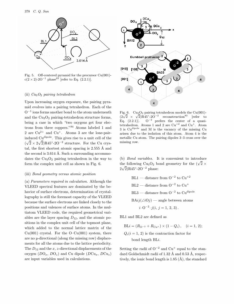
(ii) Cu3O2 pairing tetrahedron
Upon increasing oxygen exposure, the pairing pyra-
mid evolves into a pairing tetrahedron. Each of the
O−1 ions forms another bond to the atom underneath
and the Cu3O2 pairing-tetrahedron structure forms,
being a case in which “two oxygens get four elec-
trons from three coppers.”84 Atoms labeled 1 and
2 are Cu2+ and Cu+. Atoms 3 are the lone-pair-
induced Cudipole. This gives rise to a unit cell of the
(√
2 × 2√
2)R45◦-2O−2 structure. For the Cu crys-
tal, the first shortest atomic spacing is 2.555 A and
the second is 3.614 A. Such a surrounding accommo-
dates the Cu3O2 pairing tetrahedron in the way to
form the complex unit cell as shown in Fig. 6.
(iii) Bond geometry versus atomic position
(a) Parameters required in calculation. Although the
VLEED spectral features are dominated by the be-
havior of surface electrons, determination of crystal-
lography is still the foremost capacity of the VLEED
because the surface electrons are linked closely to the
positions and valences of surface atoms. In the mul-
tiatom VLEED code, the required geometrical vari-
ables are the layer spacing D12, and the atomic po-
sitions in the complex unit cell of the topmost plane,
which added to the normal lattice matrix of the
Cu(001) crystal. For the O–Cu(001) system, there
are no y-directional (along the missing row) displace-
ments for all the atoms due to the lattice periodicity.
TheD12 and the x, z-directional displacements of the
oxygen (DOx, DOz) and Cu dipole (DCux, DCuz)
are input variables used in calculations.
�� � � � �� � � � �
� � � � �
�
��
�
�
�
�
�
�
�
�
� �
� � �
� � �
� � � �� � �
�
�
�
�
� � � �
� � � �
!"
# $"
% &'
(
) * + , , - . . / 0 1 2 0 * 3 4 1 5
(
Fig. 6. Cu3O2 pairing tetrahedron models the Cu(001)-(2√
2 ×√
2)R45◦-2O−2 reconstruction83 [refer toEq. (2.2.1)]. O−2 prefers the center of a quasi-tetrahedron. Atoms 1 and 2 are Cu+2 and Cu+. Atom3 is Cudipole and M is the vacancy of the missing Cuarisen due to the isolation of this atom. Atom 4 is themetallic Cu atom. The pairing dipoles 3–3 cross over themissing row.
(b) Bond variables. It is convenient to introduce
the following Cu3O2 bond geometry for the (√
2 ×2√
2)R45◦-2O−2 phase:
BL1 — distance from O−2 to Cu+2
BL2 — distance from O−2 to Cu+
BL3 — distance from O−2 to Cudipole
BAij(∠iOj) — angle between atoms
i–O−2–j(i, j = 1, 2, 3) .
BL1 and BL2 are defined as
BLi = (RO−2 +RCu+)× (1−Qi) , (i = 1, 2);
Qi(i = 1, 2) is the contraction factor for
bond length BLi.
Setting the radii of O−2 and Cu+ equal to the stan-
dard Goldschmidt radii of 1.32 A and 0.53 A, respec-
tively, the ionic bond length is 1.85 (A), the standard
O–Cu(001): I. Binding the Signatures of LEED, STM and PES in a Bond-Forming Way 379
value for the Cu2O bulk. The effective CNs of Cu+2
and Cu+ are taken as 4 and 6, respectively. So the
corresponding contracting coefficients are Q1 = 12%
and Q2 = 4%. Thus the lengths of contracting ionic
bonds are
BL1 = 1.85× (1.00− 0.12) = 1.628 (A) ,
BL2 = 1.85× (1.00− 0.04) = 1.776 (A) .
The bond angle BA12 is constrained to be 104.5◦
or less. BA33 can be any value greater than 109.5◦
due to the strong repulsion between the lone pairs
and between the dipoles. In calculations using this
model for the kinetic processes, Q2 is taken as
an adjustable variable, while Q1(= 0.12) is always
assumed to be a constant because the first bond
forms immediately upon oxygen-molecule dissocia-
tion. Thus the variables of Q2, DCux and BA12 are
the important ones in determining the collective mo-
tion of the atoms in a complex unit cell during the
reaction.
Change of the variables (DCux = 0.25± 0.25 A;
BA12 ≤ 104.5◦; Q2 = 0.04 ± 0.04) is independent
and is restricted to finite intervals. This differs from
the atomic-shift wisdom, in which one has to con-
sider the atomic dislocation in one direction at one
time. The calculation advantage of such a set of vari-
ables is that the number of the adjustable variables
is reduced from the conventional five to two (for a
stable system) or three (for a kinetic system), and
the bond geometry is clearly constrained by physi-
cal principles. As will be demonstrated, any single
variation of these variables will affect almost all the
atoms in a single unit cell. The advantage of us-
ing these variables is not only that they reconcile
all the simultaneously geometrical variations due to
bond formation, but also that this treatment avoids
adjusting individual atomic positions in calculations.
Furthermore, in a real system, any individual atomic
shift will in principle affect other atoms of the entire
system. In other words, the bond geometry is more
realistic and convenient than the atomic-disposition
wise.
(c) Transformation of the variables. All the struc-
tural parameters (D12, DOx, DOz, DCux and
DCuz) required in calculation can be determined
by the bond geometry (Q1, Q2, DCux and BA12).
DCux, together with DCuz, determines the orien-
tation and the distance between the Cudipole and
�
����� ��� � ���� ��� �� � � � � �
�
�
�
�
�
� ���
����
����
�
� �
�
�
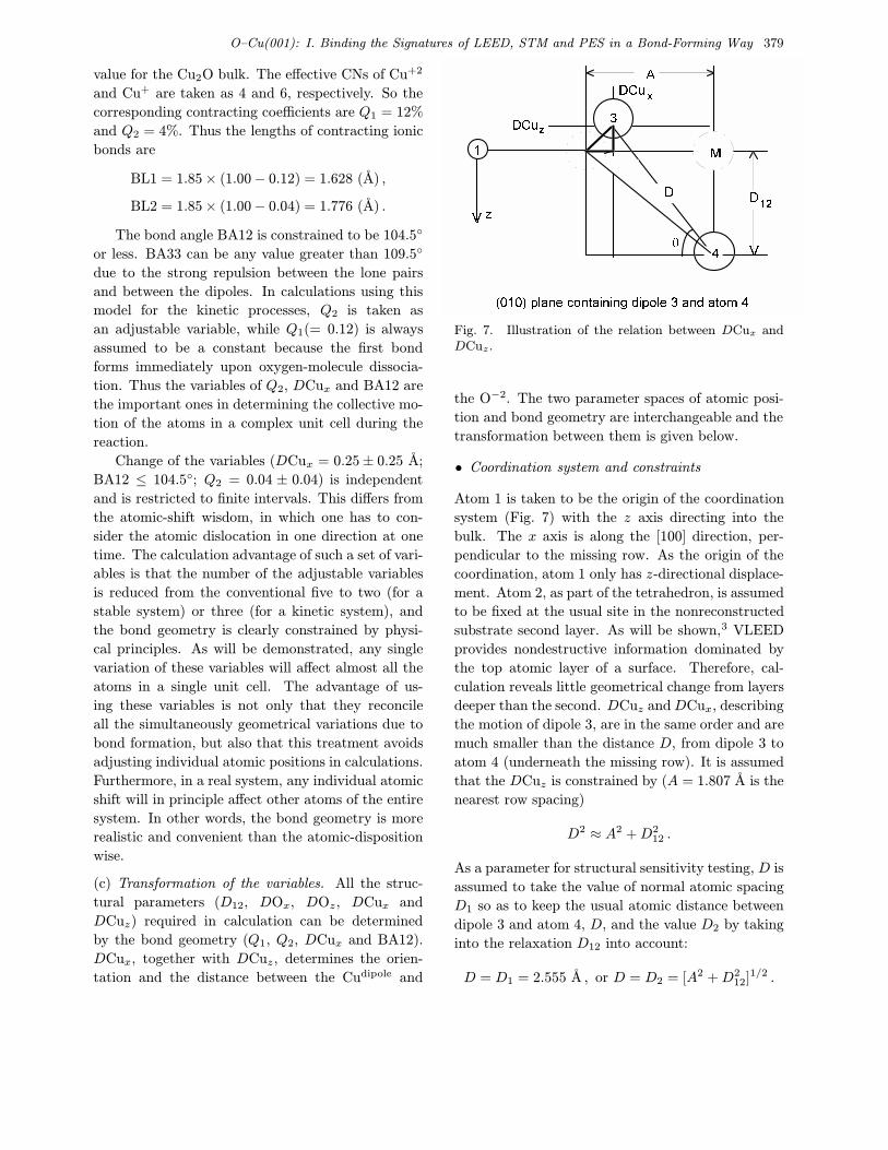
Fig. 7. Illustration of the relation between DCux andDCuz.
the O−2. The two parameter spaces of atomic posi-
tion and bond geometry are interchangeable and the
transformation between them is given below.
• Coordination system and constraints
Atom 1 is taken to be the origin of the coordination
system (Fig. 7) with the z axis directing into the
bulk. The x axis is along the [100] direction, per-
pendicular to the missing row. As the origin of the
coordination, atom 1 only has z-directional displace-
ment. Atom 2, as part of the tetrahedron, is assumed
to be fixed at the usual site in the nonreconstructed
substrate second layer. As will be shown,3 VLEED
provides nondestructive information dominated by
the top atomic layer of a surface. Therefore, cal-
culation reveals little geometrical change from layers
deeper than the second. DCuz andDCux, describing
the motion of dipole 3, are in the same order and are
much smaller than the distance D, from dipole 3 to
atom 4 (underneath the missing row). It is assumed
that the DCuz is constrained by (A = 1.807 A is the
nearest row spacing)
D2 ≈ A2 +D212 .
As a parameter for structural sensitivity testing, D is
assumed to take the value of normal atomic spacing
D1 so as to keep the usual atomic distance between
dipole 3 and atom 4, D, and the value D2 by taking
into the relaxation D12 into account:
D = D1 = 2.555 A , or D = D2 = [A2 +D212]1/2 .
380 C. Q. Sun
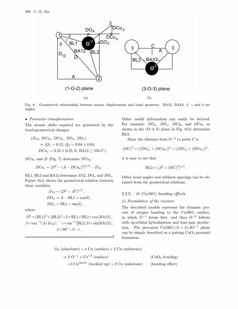
�
�
�
�
���
�������
���
�
���
�
��
���
��
�
��
����� ������
��
����� ������
� ��
��
���
��� ����
(a) (b)
Fig. 8. Geometrical relationship between atomic displacement and bond geometry. BA12, BA33, β, γ and δ areangles.
• Parameter transformation
The atomic shifts required are generated by the
bond-geometrical changes:
(D12, DCux, DCuz, DOx, DOz)
⇒ (Q1 = 0.12, Q2 = 0.04± 0.04,
DCux = 0.25± 0.25 A, BA12 ≤ 104.5◦) .
DCux and D (Fig. 7) determine DCuz:
DCuz = [D2 − (A−DCux)2]1/2 −D12 .
BL1, BL2 and BA12 determine D12, DOx and DOz.
Figure 8(a) shows the geometrical relation between
these variables:
D12 = (D2 −A2)1/2 ,
DOx = A− BL1× cos(δ) ,
DOz = BL1× sin(δ) ,
where
D2 =(BL1)2+(BL2)2+2×BL1×BL2×cos (BA12) ,
β=tan−1(A/D12) ; γ=sin−1[BL2/D×sin(BA12)] ;
δ=90◦−β−γ .
Other useful information can easily be derived.
For example, DOx, DOz, DCux and DCuz as
shown in the (O–3–3) plane in Fig. 8(b) determine
BL3.
Since the distance from O−2 to point C is
(OC)2
= (|DOx|+ |DCux|)2 + (|DOz|+ |DCuz|)2 ,
it is easy to see that
BL3 = [A2 + (OC)2]1/2 .
Other bond angles and sublayer spacings can be ob-
tained from the geometrical relations.
2.2.5. O–Cu(001) bonding effects
(i) Formulation of the reaction
The described models represent the dynamic pro-
cess of oxygen bonding to the Cu(001) surface,
in which O−1 forms first, and then O−2 follows
with sp-orbital hybridization and lone-pair produc-
tion. The precursor Cu(001)-(2 × 2)-2O−1 phase
can be simply described as a pairing CuO2 pyramid
formation:
O2 (adsorbate) + 4 Cu (surface) + 2 Cu (substrate)
⇒ 2 O−1 + Cu+2 (surface) (CuO2 bonding)
+3 Cudipole (buckled up) + 2 Cu (substrate) (bonding effect).
O–Cu(001): I. Binding the Signatures of LEED, STM and PES in a Bond-Forming Way 381
The MR type Cu(001)-(√
2×2√
2)R45◦-2O−2 structure is a consequence of the pairing CuO2 pyramid evolvinginto a pairing-tetrahedron Cu3O2:
⇒ 2 O−2 (hybrid) + Cu+2 (surface) + 2 Cu+ (substrate) (Cu3O2 bonding)
+2 Cudipole (buckled up) + Cu (MR vacancy) (bonding effect). (2.2.1)
It is to be noted that only the bonding effects such
as the MR vacancies and the buckled Cudipole are
observable in reality, while the origin of the phenom-
ena, the kinetic process of bond forming, is so far by
no means detectable.
(ii) Surface atomic valences
The adaptation of the primary-bond model to the
O–Cu(001) system improves our understanding in
that:
• Atomic dispositions are determined by the bond
geometry. The first-interlayer distance expands
depending on the bond geometry (BL1, BL2 and
BA12). The second-layer spacing contracts due to
the alternation of valences of atoms in the second
layer. Interaction between ion and metal should
be stronger than that between metal and metal.
• Atomic sizes and valences change during the re-
action. Oxygen adsorption is the process of bond
forming, which gives rise to Cu+2, Cu+, O−1 and
O−2 and the lone-pair-induced Cudipole as well as
the missing-row Cu vacancy. The Cu3O2 struc-
ture creates three sublayers and six different rows
in a complex unit cell. The top first sublayer is
composed of Cudipole with dimension expansion;
the second sublayer is of Cu+2 ions with radii con-
traction and lowering of energy states; the third
sublayer is composed of O−2 hybrids. Both Cu+2
and O−2 ions are detected as depressions with an
STM due to the relatively lowered energy states.
Along the [100] direction, on each side of the miss-
ing row, there is a Cudipole row, an O−2 row and a
Cu+2 row. The Cudipole row displaces outward
and close to the missing row. The Cu2+ row
pairs two Cudipole rows. The (Cudipole · · ·Cudipole)
forms an antibonding quadruple that bridges over
the missing row, which should be responsible for
the “dumbbell” protrusion in the STM image and
reduction of the work function.
• Clearly, O−2 prefers the nearly central position of
the M2O tetrahedron rather than an apical site of
the tetrahedron. Therefore, O−2 is located under-
neath the top layer and close to atom 1 due to the
bond contraction. The shortened distance from
O−2 to atom 1 (Cu+2) has ever been excluded in
earlier modeling considerations.85
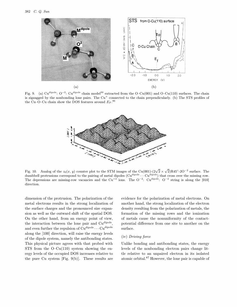
• The O–Cu–O string, as shown in Fig. 9, is
zigzagged by electron lone pairs (Cudipole: O−2:
Cudipole) rather than other kinds of bonding or
antibonding states. The missing-row atom is pro-
duced by the isolation of this atom from other
neighbors during the bond forming. As can be
seen from Fig. 6, all neighbors of the M atom have
bonded to the adsorbate.
(iii) Bond network and STM signatures
The surface bond network can be constructed by
repeatedly packing the complex unit cell. The ob-
served Cu dipoles in the O–Cu–O chains are not
those (1 and 2) belonging to the Cu2O system (see
Fig. 9). Those belonging to the Cu2O molecule are
perpendicularly connected to the O–Cu chain and
they cannot be detected by STM because of the ra-
dius reduction (from 1.27 A to 0.53 A) and elec-
tronic hole production below EF . Also shown in
Fig. 9(b) are the STS profiles measured along the
O–Cu chain at different sites from the Cu(110) sur-
face. Figure 10 gives an analog of the STM image
for the O−2-induced Cu(001) surface reconstruction.
It is to be noted that the STM image37 of a clean
Cu(001) surface did not show any overlap of the elec-
tron cloud though the atomic spacing is 2.555 A.
This distance is much shorter than that between the
pairing chains, which is estimated at 2.9± 0.3 A, of
the O–Cu(001) surface. However, the pronounced
dumbbell protrusions cross over the missing row.
In the constant-current mode, the STM protrusions
are maps of spatial DOS sampled at a potential re-
lated to the voltage applied between the tip and the
sample. Therefore, a rigid-sphere model can hardly
reveal the underlying mechanism of such a big pro-
trusion. However, this kind of protrusion is readily
accounted for from the bond-formation point of view.
From a spatial point of view, the displacement of
the ion-core position and the shift of the charge cen-
ters of the lone-pair-induced dipoles determine the
382 C. Q. Sun
(a)
� � � � � � � � � � � � � � � �
�
��
��
� � �
� � � � � � � � � �
!
(b)
Fig. 9. (a) Cudipole: O−2: Cudipole chain model50 extracted from the O–Cu(001) and O–Cu(110) surfaces. The chainis zigzagged by the nonbonding lone pairs. The Cu+ connected to the chain perpendicularly. (b) The STS profiles ofthe Cu–O–Cu chain show the DOS features around EF .86
Fig. 10. Analog of the z0(x, y) counter plot to the STM images of the Cu(001)-(2√
2×√
2)R45◦-2O−2 surface. Thedumbbell protrusions correspond to the pairing of metal dipoles (Cudipole · · ·Cudipole) that cross over the missing row.The depressions are missing-row vacancies and the Cu+2 ions. The O−2: Cudipole: O−2 string is along the [010]direction.
dimension of the protrusion. The polarization of the
metal electrons results in the strong localization of
the surface charges and the pronounced size expan-
sion as well as the outward shift of the spatial DOS.
On the other hand, from an energy point of view,
the interaction between the lone pair and Cudipole,
and even further the repulsion of Cudipole · · ·Cudipole
along the [100] direction, will raise the energy levels
of the dipole system, namely the antibonding states.
This physical picture agrees with that probed with
STS from the O–Cu(110) system showing the en-
ergy levels of the occupied DOS increases relative to
the pure Cu system [Fig. 9(b)]. These results are
evidence for the polarization of metal electrons. On
another hand, the strong localization of the electron
density resulting from the polarization of metals, the
formation of the missing rows and the ionization
of metals cause the nonuniformity of the contact-
potential difference from one site to another on the
surface.
(iv) Driving force
Unlike bonding and antibonding states, the energy
levels of the nonbonding electron pairs change lit-
tle relative to an unpaired electron in its isolated
atomic orbital.87 However, the lone pair is capable of
O–Cu(001): I. Binding the Signatures of LEED, STM and PES in a Bond-Forming Way 383
polarizing the neighboring metal atoms. Therefore,
the centers of the negative and positive charges of
the dipoles shift oppositely along the resultant di-
rection at which the two lone pairs are acting. The
strength of interaction for an O−2 : Cudipole : O−2
system is twice that of a single hydrogen bond. It
is known that the hydrogen bond is weaker than
the van der Waals bond (∼−0.1 eV/atom) and even
weaker than the ionic (∼−3.0 eV/atom) or covalent
(∼−7.0 eV/atom) bond. The processes of form-
ing the contracting ionic bonds (∼−3.0/(1 −Qi) eV/atom)80 and breaking the metallic bond
(∼−1.0 eV/atom) release energy:
∆E = −1.0− [−3.0/(1−Qi)]
= (2.0 +Qi)/(1−Qi) (eV/atom) . (2.2.2)
Such an amount of energy contributes to the
hybridization of the sp orbitals of oxygen. The
hybridization of the sp orbitals further lowers
the system energy. These energies provide forces
driving the reconstruction and missing-row forma-
tion. Besides, the resultant repulsive forces of the
lone pairs supply disturbance for the missing-row for-
mation. These forces work on the Cu atoms that
have been isolated during the oxide bond formation
and finally drive them away. As a consequence of the
metallic bond breaking, H-bond-like and contracting
ionic bonds form and the missing-row atoms are then
squeezed away by the disturbance of the repulsion.
One can describe the formation of the missing row by
the analogy that this is like digging the earth around
and cutting the roots of a tree prior to pulling it out
of the ground.
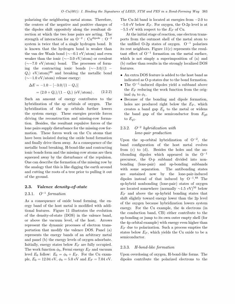
2.3. Valence density-of-state
2.3.1. O−1 formation
As a consequence of oxide bond forming, the en-
ergy band of the host metal is modified with addi-
tional features. Figure 11 illustrates the evolution
of the density-of-state (DOS) in the valence band,
or above the vacuum level, of the host. Arrows
represent the dynamic processes of electron trans-
portation that modify the valence DOS. Panel (a)
represents the energy bands of an arbitrary metal
and panel (b) the energy levels of oxygen adsorbate.
Initially, energy states below EF are fully occupied.
The work function φ0, Fermi energy EF and vacuum
level E0 follow: E0 = φ0 + EF . For the Cu exam-
ple, E0 = 12.04 eV, φ0 = 5.0 eV and EF = 7.04 eV.
The Cu-3d band is located at energies from −2.0 to
−5.0 eV below EF . For oxygen, the O-2p level is at
−5.5 eV with respect to the EF of Cu.
At the initial stage of reaction, one electron trans-
ports from the outmost shell of the metal atom to
the unfilled O-2p states of oxygen. O−1 polarizes
its rest neighbors. Figure 11(c) represents the resul-
tant effect of O−1 formation on the metal surface,
which is not simply a superimposition of (a) and
(b) rather than results in the strongly localized DOS
features.
• An extra DOS feature is added to the host band as
indicated as O-p states due to the bond formation.
• The O−1-induced dipoles yield a subband above
the EF reducing the work function from the orig-
inal φ0 to φ1.
• Because of the bonding and dipole formation,
holes are produced right below the EF , which
creates a band gap Eg to the metal or widens
the band gap of the semiconductor from Eg0to Eg1.
2.3.2. O−2 hybridization withlone-pair production
Upon the sp-orbital hybridization of O−2, the
band configuration of the host metal evolves
from (c) to (d). Besides the holes and the an-
tibonding dipoles which appeared in the O−1
precursor, the O-p subband divided into non-
bonding (lone-pair) and sp-bonding subbands
with some separation. The antibonding states
are sustained now by the lone-pair-induced
dipoles instead of that induced by O−1.88 The
sp-hybrid nonbonding (lone-pair) states of oxygen
are located somewhere (normally ∼1.5 eV)50 below
EF and above the sp-hybrid bonding states that
shift slightly toward energy lower than the 2p level
of the oxygen because hybridization lowers system
energy. For the Cu example, the 4s electrons (in
the conduction band, CB) either contribute to the
sp-bonding or jump to its own outer empty shell (for
the 4p orbital example) with energy even higher than
EF due to polarization. Such a process empties the
states below EF , which yields the Cu oxide to be a
semiconductor.
2.3.3. H-bond-like formation
Upon overdosing of oxygen, H-bond-like forms. The
dipoles contribute the polarized electrons to the
384 C. Q. Sun
�
��
���
��
��
��
��
��
��
��
���� �� ��������
����� � ��
�
���
�
���
��
�
��
��
��
��
���
�� ��������
�
���� � ��
�
���
�
��
�
� �
��
��
��
��
� ����������
�� ��������� �
�
����������
�������� �������� �� ��
Fig. 11. Valence-DOS modification of the metal surface with chemisorbed oxygen. Panel (a) and panel (b) correspondto the valence band of pure metal and oxygen, respectively. The O-2p level is much lower than the EF of the metal.Panel (c) shows the result of O adding to metal at the initial stage of reaction. O−1 formation produces holes andantibonding dipoles. Panel (d) corresponds to the effect of O−2 formation, which gives rise to four characteristicsubband features that are all localized.88,100
bonding orbitals of additional oxygen adsorbate.
The arrow from the antibonding states to the
sp-bonding subband represents the process of the
H-bond-like formation. STS and VLEED revealed
that the states of antibonding of the O–Cu system
range over 1.3 ± 0.5 eV and the nonbonding states
−2.1± 0.7 eV around EF . The PEEM studies of O–
Pt surfaces89,90 detected the conversion of the dark
islands, in the scale of 102µm, into very bright ones
with work functions ∼1.2 eV lower than that of the
clean surface.
2.4. 3D surface potential barrier
2.4.1. Initiatives
The surface potential barrier (SPB) reflects the
charge distribution both in real space and in energy
space,4,6 which is linked to the change of valences and
geometrical arrangement of atoms of the surface.91
For a clean metal system, such as Cu(001),1,52,92
W(001)93–95 and Ru(110)15,21 as well as Ni,14,96
the SPB has been modeled successfully as a uni-
form layer of thin-film interference. The inelastic
O–Cu(001): I. Binding the Signatures of LEED, STM and PES in a Bond-Forming Way 385
damping has been assumed to be monotonically
energy-dependent. STM and STS observations37,55
have provided evidence that the uniform-SPB ap-
proximation is good enough for clean metals. For
example, STM reveals that the ion cores with small
protrusions (0.15–0.30 A) arrange regularly in the
homogeneous background or Fermi sea; STS studies
of the Cu(110) surface86 confirmed the uniformity of
the DOS below EF . Hence, clean metal surfaces can
be described as nearly-ideal Fermi systems and the
uniform-SPB approximation is practical and accept-
able within the error of detection.
Surfaces with chemisorbed oxygen differ much
from those of the pure metals in that the chemisorbed
surfaces possess many “rather local” properties —
varying site from site around an atom. The
chemisorption of oxygen results not only in the dis-
location of ion cores but also in the alternation of
atomic sizes and valences. More importantly, as con-
sequences of oxygen–metal bonding, the formation of
the dipole layer and, in some cases, the removal of
atoms roughen the surface. These features have been
detected with STM, PEEM, LEED, and other tech-
niques as well. Even at very low exposure to oxygen,
the Cu(001) surface is roughened by the protruding
domain boundaries; see Fig. 1(a). The STM scale
differences of the systems with chemisorbed oxygen
are much higher (0.45–1.1 A) than that of pure met-
als. The STS profiles from the O–Cu chain region on
the O–Cu(110) surface show that there is a general
elevation of energy states. In particular, the above-
EF empty surface state is occupied and a new DOS
feature is generated below EF (Fig. 9).
Furthermore, in decoding VLEED from the O–
Cu(001) surface, Thurgate and Sun1 found that the
spectrum collected at the azimuth closing to the
〈11〉 direction (perpendicular to the missing row)
could not be simulated with the uniform SPB by us-
ing either the Cu(001)-c(2 × 2)-2O−1 or the (√
2 ×2√
2)R45◦-2O−2 structure, or even their combination
with various SPB parameters. Therefore, it seemed
implausible with VLEED to simultaneously deter-
mine the SPB and the crystal structure by deal-
ing with the strongly correlated parameters inde-
pendently. The atomic-scale localization and the
on-site variation of energy states of the systems with
chemisorbed oxygen suggest that it is necessary to
consider the electron distribution on the surface site
by site. The 3D effect, the variation of energy states
of the surface and the correlation among the param-
eters used in calculations constitute the complex-
ity in decoding VLEED data from the systems with
chemisorbed oxygen.
Therefore, it is necessary to develop a
nonuniform-SPB model for the systems with
chemisorbed oxygen in order to:
• Reduce the number of independent variables in the
SPB to simplify VLEED optimization and to en-
sure the certainty of solution;
• Allow the calculation code to automatically op-
timize the z0(E) to reproduce the experimental
data;
• Let the z0(E) profiles vary with the crystal struc-
ture to reflect appropriately the interdependence
between the atomic geometry and the electronic
structures; and, eventually,
• Produce the essential DOS features in the energy
range covered by VLEED, and
• Gain deeper insight into the behavior of atoms
and electrons on metal surfaces with chemisorbed
oxygen.
2.4.2. Constraints
Electrons with energy E traversing the surface re-
gion can be described as moving in a complex optical
potential:4
V (r, E) = ReV (r) + iImV (r, E)
= ReV (r) + iIm[V (r)× V (E)] . (2.4.1)
V (r, E) satisfies the following constraints:
(i) The elastic potential, ReV (r), satisfies the
Poisson equation,97 and the gradient of ReV (r)
relates to the intensity of the electric field ε(r):
ImV (r) ∝ −∇2[ReV (r)] = ρ(r) ;
and
∇[ReV (r)] = −ε(r) .
If ρ(r) = 0, then ReV (r) corresponds to a conser-
vation field, i.e. the moving electrons will suffer no
energy loss and the spatial variation of the inelastic
damping potential ImV (r) ∝ ρ(r) = 0. Therefore,
ImV (r) and ReV (r) should not be independent and
386 C. Q. Sun
they correlate with each other uniquely through the
electron distribution ρ(r).
(ii) The energy dependence of the inelastic poten-
tial, ImV (E), reflects the effect of all the dissipative
processes that are dominated by phonon and single-
electron excitation at energies below that for plasma
excitation. This means that the single-electron ex-
citation occurs in the electron-occupied space, de-
scribed by ρ(r), and with any incident energy E
greater than the work function φ. As remarked by
Pendry,4 no contribution to ImV (E) from a particu-
lar loss mechanism can come about until the incident
electron has enough energy to excite this mechanism.
Plasma excitation needs energies around 15 eV above
EF98 in metal with a free-electron conduction band.
The contribution of plasma excitation to ImV (E)
does not come into play below this value. Even
in non-free-electron metals there is a more general
cluster of excitations usually at around the equiva-
lent free-electron plasmon energy. Below the plas-
mon energy, single electrons can still be excited from
the conduction band, though they produce smaller
ImV (E) features than plasma excitation. In met-
als, single electrons can be excited by an incident
electron that has any energy greater than the work
function (E ≥ φ), but in insulators the situation is
different. On the other hand, phonon excitation and
photon excitation may occur at energies that are
much lower than the work function. Therefore, at
energies between the work function and the plasma-
excitation threshold, single-electron excitation dom-
inates, which adds “humps” to the inelastic damping
showing the DOS distribution in this region.
(iii) The z-directional integration of ImV (z, E)
and ReV (z) corresponds, respectively, to the ampli-
tude loss ∆A and the phase change ∆Φ of the re-
flected electron beams that are described with plane
waves:
ϕ = A exp(−ik · r + Φ) ,
and
∆A ∝∫ −∞a
ϕ ImV (z, E)ϕ∗dz ,
∆Φ ∝∫ −∞a
ϕReV (z)ϕ∗dz ,
(2.4.2)
where k is the plane-wave vector. Integration starts
from a certain point, a, inside the crystal, to in-
finitely far away from the surface. The parame-
ter a varies depending on the penetration depth of
the incident beams. This constraint provides lee-
way for the mathematical expressions of ReV (z)
and ImV (z, E), as the specific forms of ImV (z),
ImV (E) and ReV (z), and therefore the exact values
of the strongly correlated parameters, are much less
important than the integration (2.4.2) in the physics.
The independent treatment of the correlation among
the SPB parameters leads to infinite numerical solu-
tions that should correspond to reality and be phys-
ically meaningful.
(iv) Most importantly, the variation in atomic ge-
ometry and the behavior of electrons, both in real
space [represented by ImV (r)] and in energy space
[described by ImV (E) or DOS], depend on each
other, as they are consequences of the surface bond
forming and the electrons connect to the sites, the
sizes and the chemical states of the atoms. There-
fore, modeling should consider the interdependence
between these identities.
2.4.3. One-dimensional SPB
The best model of ReV (z) currently in use was for-
mulated by Jones, Jennings and Jepsen in 198493
on the basis that it closely approximated the results
of jellium and density functional calculations of the
SPB. This model has widely been used for the fit-
ting both of the VLEED fine-structure features and
of the inverse-photoemission image states, and has
the form
ReV (z) =−V0
1 +A exp[−B(z − z0)], z ≥ z0 (a pseudo-Fermi z function)
=1− exp[λ(z − z0)]
4(z − z0), z < z0 (the image potential) , (2.4.3)
O–Cu(001): I. Binding the Signatures of LEED, STM and PES in a Bond-Forming Way 387
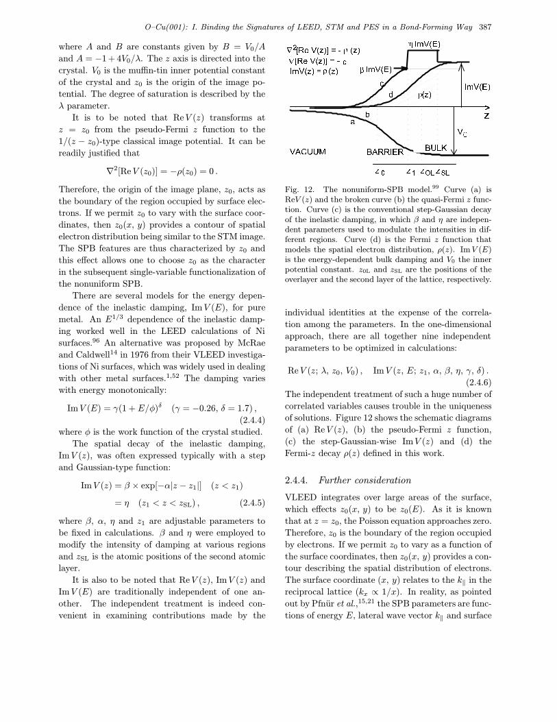
where A and B are constants given by B = V0/A
and A = −1 + 4V0/λ. The z axis is directed into the
crystal. V0 is the muffin-tin inner potential constant
of the crystal and z0 is the origin of the image po-
tential. The degree of saturation is described by the
λ parameter.
It is to be noted that ReV (z) transforms at
z = z0 from the pseudo-Fermi z function to the
1/(z − z0)-type classical image potential. It can be
readily justified that
∇2[ReV (z0)] = −ρ(z0) = 0 .
Therefore, the origin of the image plane, z0, acts as
the boundary of the region occupied by surface elec-
trons. If we permit z0 to vary with the surface coor-
dinates, then z0(x, y) provides a contour of spatial
electron distribution being similar to the STM image.
The SPB features are thus characterized by z0 and
this effect allows one to choose z0 as the character
in the subsequent single-variable functionalization of
the nonuniform SPB.
There are several models for the energy depen-
dence of the inelastic damping, ImV (E), for pure
metal. An E1/3 dependence of the inelastic damp-
ing worked well in the LEED calculations of Ni
surfaces.96 An alternative was proposed by McRae
and Caldwell14 in 1976 from their VLEED investiga-
tions of Ni surfaces, which was widely used in dealing
with other metal surfaces.1,52 The damping varies
with energy monotonically:
ImV (E) = γ(1 +E/φ)δ (γ = −0.26, δ = 1.7) ,
(2.4.4)
where φ is the work function of the crystal studied.
The spatial decay of the inelastic damping,
ImV (z), was often expressed typically with a step
and Gaussian-type function:
ImV (z) = β × exp[−α|z − z1|] (z < z1)
= η (z1 < z < zSL) , (2.4.5)
where β, α, η and z1 are adjustable parameters to
be fixed in calculations. β and η were employed to
modify the intensity of damping at various regions
and zSL is the atomic positions of the second atomic
layer.
It is also to be noted that ReV (z), ImV (z) and
ImV (E) are traditionally independent of one an-
other. The independent treatment is indeed con-
venient in examining contributions made by the
�
�
�
� � � � � �
� � � � � �
�
�
� � �
� � � � � �
� � � � � � �� � � � � � � � � ��
� !" # $ % & ' ( ) * + & ' (, - . / 0 1 2 3 4 5 6 7
8 9 : : ; < : 8 = > ?
@ A B C D E F EGG
H
I
Fig. 12. The nonuniform-SPB model.99 Curve (a) isReV (z) and the broken curve (b) the quasi-Fermi z func-tion. Curve (c) is the conventional step-Gaussian decayof the inelastic damping, in which β and η are indepen-dent parameters used to modulate the intensities in dif-ferent regions. Curve (d) is the Fermi z function thatmodels the spatial electron distribution, ρ(z). ImV (E)is the energy-dependent bulk damping and V0 the innerpotential constant. z0L and zSL are the positions of theoverlayer and the second layer of the lattice, respectively.
individual identities at the expense of the correla-
tion among the parameters. In the one-dimensional
approach, there are all together nine independent
parameters to be optimized in calculations:
ReV (z; λ, z0, V0) , ImV (z, E; z1, α, β, η, γ, δ) .
(2.4.6)
The independent treatment of such a huge number of
correlated variables causes trouble in the uniqueness
of solutions. Figure 12 shows the schematic diagrams
of (a) ReV (z), (b) the pseudo-Fermi z function,
(c) the step-Gaussian-wise ImV (z) and (d) the
Fermi-z decay ρ(z) defined in this work.
2.4.4. Further consideration
VLEED integrates over large areas of the surface,
which effects z0(x, y) to be z0(E). As it is known
that at z = z0, the Poisson equation approaches zero.
Therefore, z0 is the boundary of the region occupied
by electrons. If we permit z0 to vary as a function of
the surface coordinates, then z0(x, y) provides a con-
tour describing the spatial distribution of electrons.
The surface coordinate (x, y) relates to the k‖ in the
reciprocal lattice (kx ∝ 1/x). In reality, as pointed
out by Pfnur et al.,15,21 the SPB parameters are func-
tions of energy E, lateral wave vector k‖ and surface
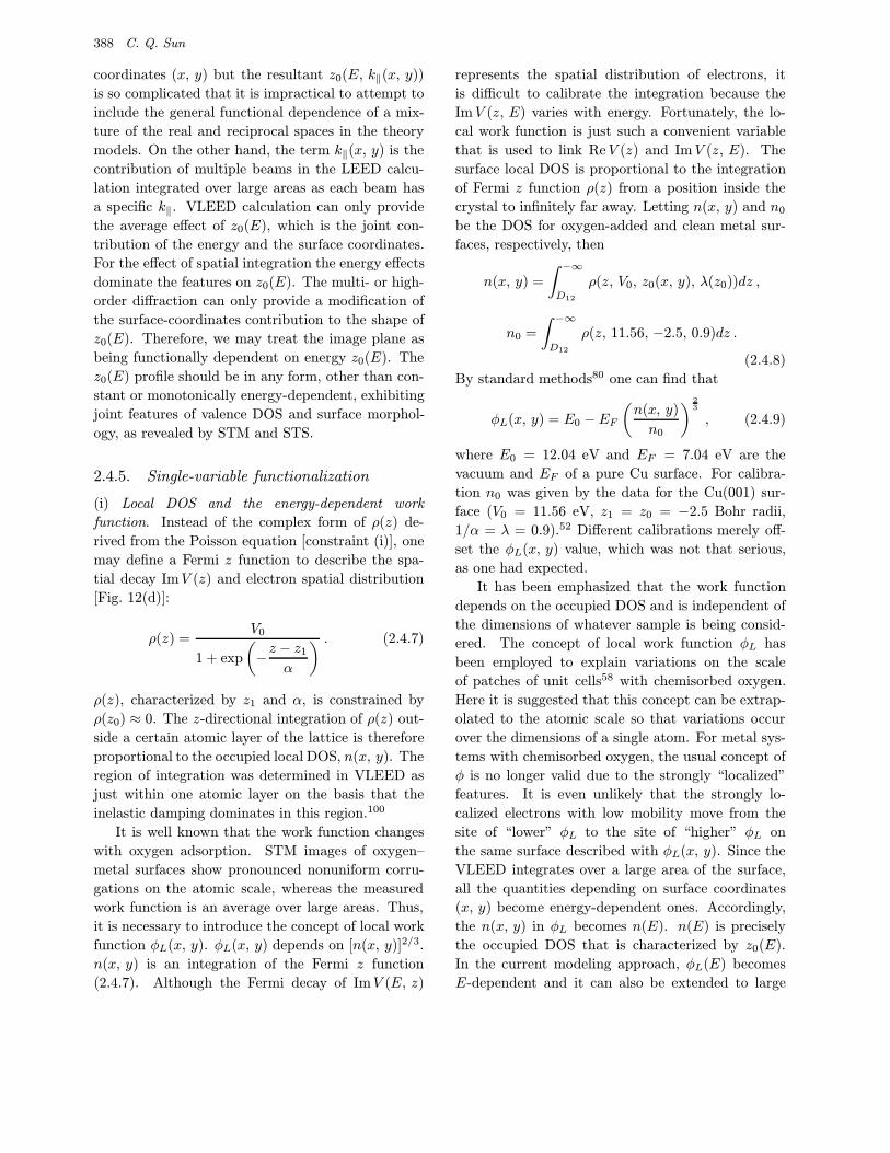
388 C. Q. Sun
coordinates (x, y) but the resultant z0(E, k‖(x, y))
is so complicated that it is impractical to attempt to
include the general functional dependence of a mix-
ture of the real and reciprocal spaces in the theory
models. On the other hand, the term k‖(x, y) is the
contribution of multiple beams in the LEED calcu-
lation integrated over large areas as each beam has
a specific k‖. VLEED calculation can only provide
the average effect of z0(E), which is the joint con-
tribution of the energy and the surface coordinates.
For the effect of spatial integration the energy effects
dominate the features on z0(E). The multi- or high-
order diffraction can only provide a modification of
the surface-coordinates contribution to the shape of
z0(E). Therefore, we may treat the image plane as
being functionally dependent on energy z0(E). The
z0(E) profile should be in any form, other than con-
stant or monotonically energy-dependent, exhibiting
joint features of valence DOS and surface morphol-
ogy, as revealed by STM and STS.
2.4.5. Single-variable functionalization
(i) Local DOS and the energy-dependent work
function. Instead of the complex form of ρ(z) de-
rived from the Poisson equation [constraint (i)], one
may define a Fermi z function to describe the spa-
tial decay ImV (z) and electron spatial distribution
[Fig. 12(d)]:
ρ(z) =V0
1 + exp
(−z − z1
α
) . (2.4.7)
ρ(z), characterized by z1 and α, is constrained by
ρ(z0) ≈ 0. The z-directional integration of ρ(z) out-
side a certain atomic layer of the lattice is therefore
proportional to the occupied local DOS, n(x, y). The
region of integration was determined in VLEED as
just within one atomic layer on the basis that the
inelastic damping dominates in this region.100
It is well known that the work function changes
with oxygen adsorption. STM images of oxygen–
metal surfaces show pronounced nonuniform corru-
gations on the atomic scale, whereas the measured
work function is an average over large areas. Thus,
it is necessary to introduce the concept of local work
function φL(x, y). φL(x, y) depends on [n(x, y)]2/3.
n(x, y) is an integration of the Fermi z function
(2.4.7). Although the Fermi decay of ImV (E, z)
represents the spatial distribution of electrons, it
is difficult to calibrate the integration because the
ImV (z, E) varies with energy. Fortunately, the lo-
cal work function is just such a convenient variable
that is used to link ReV (z) and ImV (z, E). The
surface local DOS is proportional to the integration
of Fermi z function ρ(z) from a position inside the
crystal to infinitely far away. Letting n(x, y) and n0
be the DOS for oxygen-added and clean metal sur-
faces, respectively, then
n(x, y) =
∫ −∞D12
ρ(z, V0, z0(x, y), λ(z0))dz ,
n0 =
∫ −∞D12
ρ(z, 11.56, −2.5, 0.9)dz .
(2.4.8)
By standard methods80 one can find that
φL(x, y) = E0 −EF(n(x, y)
n0
) 23
, (2.4.9)
where E0 = 12.04 eV and EF = 7.04 eV are the
vacuum and EF of a pure Cu surface. For calibra-
tion n0 was given by the data for the Cu(001) sur-
face (V0 = 11.56 eV, z1 = z0 = −2.5 Bohr radii,
1/α = λ = 0.9).52 Different calibrations merely off-
set the φL(x, y) value, which was not that serious,
as one had expected.
It has been emphasized that the work function
depends on the occupied DOS and is independent of
the dimensions of whatever sample is being consid-
ered. The concept of local work function φL has
been employed to explain variations on the scale
of patches of unit cells58 with chemisorbed oxygen.
Here it is suggested that this concept can be extrap-
olated to the atomic scale so that variations occur
over the dimensions of a single atom. For metal sys-
tems with chemisorbed oxygen, the usual concept of
φ is no longer valid due to the strongly “localized”
features. It is even unlikely that the strongly lo-
calized electrons with low mobility move from the
site of “lower” φL to the site of “higher” φL on
the same surface described with φL(x, y). Since the
VLEED integrates over a large area of the surface,
all the quantities depending on surface coordinates
(x, y) become energy-dependent ones. Accordingly,
the n(x, y) in φL becomes n(E). n(E) is precisely
the occupied DOS that is characterized by z0(E).
In the current modeling approach, φL(E) becomes
E-dependent and it can also be extended to large
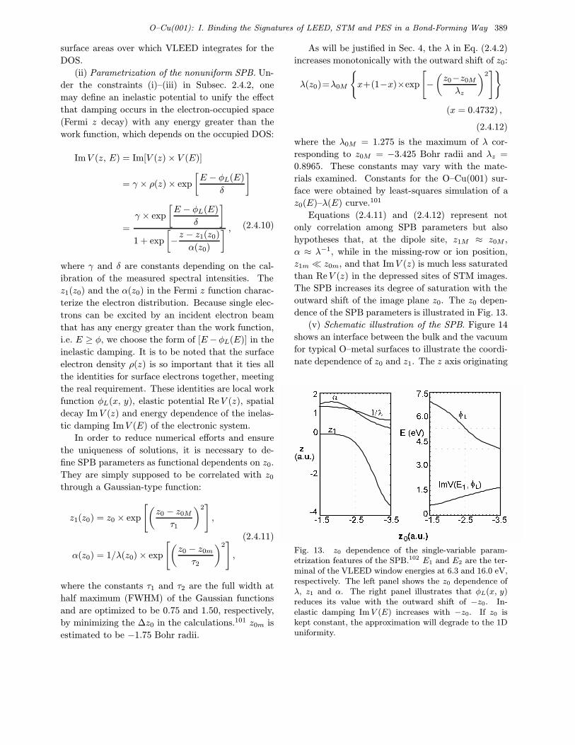
O–Cu(001): I. Binding the Signatures of LEED, STM and PES in a Bond-Forming Way 389
surface areas over which VLEED integrates for the
DOS.
(ii) Parametrization of the nonuniform SPB. Un-
der the constraints (i)–(iii) in Subsec. 2.4.2, one
may define an inelastic potential to unify the effect
that damping occurs in the electron-occupied space
(Fermi z decay) with any energy greater than the
work function, which depends on the occupied DOS:
ImV (z, E) = Im[V (z)× V (E)]
= γ × ρ(z)× exp
[E − φL(E)
δ
]
=
γ × exp
[E − φL(E)
δ
]1 + exp
[−z − z1(z0)
α(z0)
] , (2.4.10)
where γ and δ are constants depending on the cal-
ibration of the measured spectral intensities. The
z1(z0) and the α(z0) in the Fermi z function charac-
terize the electron distribution. Because single elec-
trons can be excited by an incident electron beam
that has any energy greater than the work function,
i.e. E ≥ φ, we choose the form of [E −φL(E)] in the
inelastic damping. It is to be noted that the surface
electron density ρ(z) is so important that it ties all
the identities for surface electrons together, meeting
the real requirement. These identities are local work
function φL(x, y), elastic potential ReV (z), spatial
decay ImV (z) and energy dependence of the inelas-
tic damping ImV (E) of the electronic system.
In order to reduce numerical efforts and ensure
the uniqueness of solutions, it is necessary to de-
fine SPB parameters as functional dependents on z0.
They are simply supposed to be correlated with z0
through a Gaussian-type function:
z1(z0) = z0 × exp
[(z0 − z0M
τ1
)2],
α(z0) = 1/λ(z0)× exp
[(z0 − z0m
τ2
)2],
(2.4.11)
where the constants τ1 and τ2 are the full width at
half maximum (FWHM) of the Gaussian functions
and are optimized to be 0.75 and 1.50, respectively,
by minimizing the ∆z0 in the calculations.101 z0m is
estimated to be −1.75 Bohr radii.
As will be justified in Sec. 4, the λ in Eq. (2.4.2)
increases monotonically with the outward shift of z0:
λ(z0)=λ0M
{x+(1−x)×exp
[−(z0−z0M
λz
)2]}
(x = 0.4732) ,
(2.4.12)
where the λ0M = 1.275 is the maximum of λ cor-
responding to z0M = −3.425 Bohr radii and λz =
0.8965. These constants may vary with the mate-
rials examined. Constants for the O–Cu(001) sur-
face were obtained by least-squares simulation of a
z0(E)–λ(E) curve.101
Equations (2.4.11) and (2.4.12) represent not
only correlation among SPB parameters but also
hypotheses that, at the dipole site, z1M ≈ z0M ,
α ≈ λ−1, while in the missing-row or ion position,
z1m � z0m, and that ImV (z) is much less saturated
than ReV (z) in the depressed sites of STM images.
The SPB increases its degree of saturation with the
outward shift of the image plane z0. The z0 depen-
dence of the SPB parameters is illustrated in Fig. 13.
(v) Schematic illustration of the SPB. Figure 14
shows an interface between the bulk and the vacuum
for typical O–metal surfaces to illustrate the coordi-
nate dependence of z0 and z1. The z axis originating
�
�
��
�
�
��
������ ���� ���
�� ������
�
��
��
���
��
���
����� ���� ���
� ���
���� ����
�������
������ � �
Fig. 13. z0 dependence of the single-variable param-etrization features of the SPB.102 E1 and E2 are the ter-minal of the VLEED window energies at 6.3 and 16.0 eV,respectively. The left panel shows the z0 dependence ofλ, z1 and α. The right panel illustrates that φL(x, y)reduces its value with the outward shift of −z0. In-elastic damping ImV (E) increases with −z0. If z0 iskept constant, the approximation will degrade to the 1Duniformity.
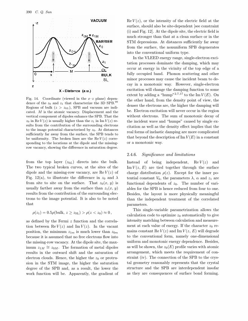
390 C. Q. Sun
�
� � ������ �� � �
��
���� ��
�
�
���
��
��
��
�
�
�������
��
�
� ����
�������
�
�
�
�
��
Fig. 14. Coordinate (viewed in the x–z plane) depen-dence of the z0 and z1 that characterize the 3D SPB.99
Regions of bulk (z > z0L), SPB and vacuum are indi-cated. M is the atomic vacancy. Displacement and thevertical component of dipoles enhance the SPB. That thez0 in ReV (z) is usually higher than the z1 in ImV (z) re-sults from the contribution of the surrounding electronsto the image potential characterized by z0. At distancessufficiently far away from the surface, the SPB tends tobe uniformity. The broken lines are the ReV (z) corre-sponding to the locations at the dipole and the missing-row vacancy, showing the difference in saturation degree.
from the top layer (z0L) directs into the bulk.
The two typical broken curves, at the sites of the
dipole and the missing-row vacancy, are ReV (z) of
Fig. 12(a), to illustrate the difference in z0 and λ
from site to site on the surface. That z0(x, y) is
usually farther away from the surface than z1(x, y)
results from the contribution of the surrounding elec-
trons to the image potential. It is also to be noted
that
ρ(z1) = 0.5ρ(bulk, z ≥ zSL) > ρ(z < z0) ≈ 0 ,
as defined by the Fermi z function and the correla-
tion between ReV (z) and ImV (z). In the vacant
position, the minimum z1m is much lower than z0m
because it is assumed that no free electrons flow into
the missing-row vacancy. At the dipole site, the max-
imum z1M∼= z0M . The formation of metal dipoles
results in the outward shift and the saturation of
electron clouds. Hence, the higher the z0 or protru-
sion in the STM image, the higher the saturation
degree of the SPB and, as a result, the lower the
work function will be. Apparently, the gradient of
ReV (z), or the intensity of the electric field at the
surface, should also be site-dependent [see constraint
(i) and Fig. 12]. At the dipole site, the electric field is
much stronger than that at a clean surface or in the
STM depressions. At distances sufficiently far away
from the surface, the nonuniform SPB degenerates
into the conventional uniform type.
In the VLEED energy range, single-electron exci-
tation processes dominate the damping, which may
occur at energy in the vicinity of the top edge of a
fully occupied band. Phonon scattering and other
minor processes may cause the incident beam to de-
cay in a monotonic way. However, single-electron
excitation will change the damping function to some
extent by adding a “hump”2,7,17 to the ImV (E). On
the other hand, from the density point of view, the
denser the electrons are, the higher the damping will
be. Electron excitation will never occur in the region
without electrons. The sum of monotonic decay of
the incident wave and “humps” caused by single ex-
citation as well as the density effect implies that the
real forms of inelastic damping are more complicated
that beyond the description of ImV (E) in a constant
or a monotonic way.
2.4.6. Significance and limitations
Instead of being independent, Re V (z) and
ImV (z, E) are tied together through the surface
charge distribution ρ(z). Except for the inner po-
tential constant V0, the parameters λ, α and z1 are
functional dependents of z0. The number of vari-
ables for the SPB is hence reduced from four to one.
Besides, the layout is more physically meaningful
than the independent treatment of the correlated
parameters.
This single-variable parametrization allows the
calculation code to optimize z0 automatically to give
intensity matching between calculation and measure-
ment at each value of energy. If the character z0 re-
mains constant ReV (z) and ImV (z, E) will degrade
to the conventional form, namely one-dimensional
uniform and monotonic energy dependence. Besides,
as will be shown, the z0(E) profile varies with atomic
arrangement, which meets the requirement of con-
straint (iv). The connection of the SPB to the crys-
tal geometry reasonably represents that the crystal
structure and the SPB are interdependent insofar
as they are consequences of surface bond forming.
O–Cu(001): I. Binding the Signatures of LEED, STM and PES in a Bond-Forming Way 391
It now becomes possible to determine crystal and
electronic properties simultaneously with VLEED
by analyzing the structure-dependent z0(E) profile.
Therefore, the difficulty of VLEED in conventional
wisdom has been overcome completely. On the other
hand, the variation of the energy state represented
by z0(E) is an important aspect of chemisorption
studies, which can also be probed as a result of this
approach.
However, processes such as band transition and
single electron excitation that add humps to the
monotonic damping (due to uniform DOS or con-
stant work function) are not apparent in the present
expression. Fortunately, this can be compensated
for by a z0-optimizing method based on the premise
that the work function depends on the DOS which
is whatsoever but not a constant in the energy range
of VLEED.
This set of approaches correlates the chemical
bond, the valence DOS and the SPB with all the
observations in terms of microscopy, crystallogra-
phy and spectroscopy. Its significance is that it re-
flects the essential link of the quantities in terms of
bond forming and its consequences on the behavior
of atoms and valence electrons at the surface by ap-
propriate parametrization.
3. VLEED Numerical Justification
3.1. Decoding methodology
3.1.1. Spectral digitization and calibration
Numerical processing of the measured VLEED
I–E spectra is essential to the understanding of the
physics behind the experimental observations, and
hence to justifying the models proposed. Digitiza-
tion and calibration of the experimental data are the
first stage in theory calculations. Inappropriate cali-
bration of the measured data may result in mislead-
ing conclusions, and therefore careful and reason-
able calibration of the data is important prior to the
numerical processing.
(i) Conventional way – normalizing the individ-
ual curve independently. Normally, both the exper-
imental Ie–E and the computed Ic–E spectra are
normalized through dividing the entire spectrum by
the maximum intensities, IeM and IcM , of the spe-
cific spectrum, respectively, so that the maxima of
all the normalized curves are equal to unity. Com-
parison between calculation and experimental results
is then performed with the “least-squares” R-factor
method:
R = 1−
√√√√√√N∑i=1
[Ic(Ei)− Ie(Ei)]2
N(N − 1).
Ic(Ei) and Ie(Ei) are normalized intensities at se-
lected energies Ei (step Ei−Ei−1 was usually taken
as 0.1 eV in the current exercises). EN is the high-
est energy of the VLEED spectrum. The R value
determines the degree of the agreement between
theory and measurement. For an ideal agreement,
R = 1. This convention is normally used and ac-
ceptable for qualitative simulation of a certain single
VLEED spectrum. This treatment gives information
on shape similarity between the theory and experi-
mental curves.
However, this method is not adequate for the
functionalized SPB, because it is unable to differ-
entiate the intensity among a series of I–E curves
such as those produced by varying oxygen exposure.
This treatment will surely miss important informa-
tion such as the relative variation of the spectral
intensity during the reaction.
(ii) Common-standard normalization with respect
to instrument precision. The relative intensity of
one curve to another in a complete set of dynamic
I–E spectra is also an important concern. In real-
ity, data collection is done under stable instrumen-
tal conditions.103 Therefore, it is necessary to cal-
ibrate all the experimental curves with a common
scale to all the I–E profiles. The reasonable way
is to choose one maximum IeM (Ei) from among all
of the experimental spectra to calibrate all the I–E
curves. This ensures correct information regarding
the relative change of intensities during the data
processing, because chemical reaction changes not
only the shape but also the intensity of the spec-
tra. On the other hand, as has been found,100 devia-
tions of the absolute spectral intensities from the real
status can be modulated by the damping potential
(1±0.2)×ImV (E) which determines the spectral in-
tensity. Modifying the damping constant offsets the
computed curves. Therefore, the intensity change
corresponds to the physical process that contributes
to the inelastic damping.
Digitization of VLEED spectra in the current
work was based on the following considerations:
392 C. Q. Sun
• The incident current I00 between 6.0 and 16.0 eV
was assumed to be constant within the instru-
mentation error. The inner potential constant V0
was kept constant in calculation though it varies
slightly with energy for the pure Cu(001) sur-
face in the normal LEED energies.104 The VLEED
spectra are actually active in the upper valence-
band region, i.e. 6.0–12.0 eV. Therefore, such as-
sumptions are reasonable.
• Calculations101 revealed that the (00) beam re-
flectance (I00/I0) greater than 12.5% causes se-
rious convergence problems. Measurement also
showed that the reflectivity is about 10%.105
Hence, the maximal value of I00/I0 = 10% was
assumed as the maximal reflectivity to calibrate
all of the I–E curves. In each curve, the absolute
intensity of the first and the last energy is vital to
determining the constants of γ and δ in the inelas-
tic SPB. For instance, once the SPB functions are
defined, we can solve the damping equation with
the initial conditions obtained by the orthogonal-
analysis technique.
• In the set of angule-resolved VLEED spectra, it
was assumed that no structural change occurs to
the bond geometry during the VLEED data acqui-
sition. This assumption is also acceptable because
the reaction is promoted more by increasing oxy-
gen exposure than by aging.
• Earlier data simulation for the Cu(001) surface52
provided values of V0 = 11.56 eV, z0 =
−2.5 a.u. [∼= 1.32 ≈ 1.276 A (Cu radius)] and
λ = 0.9. These data were used to calibrate the
local work function and as references for setting
the SPB parameters.
• The z-scale difference of 0.45 A in the STM
image provides reference for ∆z0 because both
the STM image and z0(x, y) are the convolu-
tion of the surface electron distribution, though
they were convoluted by different mechanisms.
Taking the lateral convolution for the finite size
of the STM tip and modification by multiple
diffraction and high-order diffraction in VLEED,
it is reasonable to assume that ∆z0 and ∆zSTM
are comparable and ∆z0 should be as small
as possible.
3.1.2. Parametrization
The first task before calculation is to determine the
constants in the SPB equations in Subsec. 2.4.
Constants in ReV (z). The orthogonal-
optimization technique was used first at several en-
ergies E0i with parameters of z0i, λi and ImV (E0i).
The least-squares method was used to fit the λ(z0)
plot for the constants. Both the STM image and
barrier distribution imply that the SPB increases its
saturation degree with the outward shift of the image
plane, z0. This provides the physical basis for the re-
lation between z0 and λ. The optimized z0M and z0m
are −3.425 and −1.750 a.u., and the corresponding
λ is 1.275 and 0.650.
Constants in ImV (z, E). There are four con-
stants in ImV (z, E). γ and δ are determined by
matching spectral intensities at the terminals of the
VLEED window (6.0 and 16.0 eV). Furnished with
the damping values at the two energies, we could
solve the damping equation to obtain the γ and δ.
The FWHM of the Gaussian functions for z1(z0) and
α(z0) are determined by obtaining the smallest ∆z0
(near the 〈11〉 direction produces the maximal value).
The numerical processing is summarized as
follows:
• SPB variables were fixed first by using the known
identities of the missing-row structure model106
and the conventional 1D SPB.1
• In order to set the constants in the single-variable
SPB functions, we calculated the VLEED data at
several energies by adjusting the most sensitive
parameters.
• Uncertainty of the solutions was overcome by
introducing the correlation among the SPB pa-
rameters as well as the local work function
(Subsec. 2.4). As will be shown, the infinite solu-
tions due to independently varying λ and z0 were
reduced to finite ones by the function of λ(z0). In-
troducing the local work function then reduced the
finite solutions to certainty.
3.1.3. Optimization method
(i) Orthogonal-optimizing method. Conventionally,
one can only change one parameter at a time in cal-
culation. Although the computer can automatically
do the numerical processing, this method is tedious
and fruitless. The orthogonal-optimizing method is
widely used in optimization for experimental design,
not only for reducing the time span of experiments
but also for predicting the trends of results and cor-
relation among the variables.
O–Cu(001): I. Binding the Signatures of LEED, STM and PES in a Bond-Forming Way 393
(ii) Z0-scanning and z0-optimizing methods. Af-
ter the SPB and geometrical parameters had been
fixed, calculations were performed based on the
single-variable parametrization by varying z0 over
−2.5 [for pure Cu(001)]±1.25 with 0.25 (a.u.) steps.
The contour plot of z0 versus E is then drawn with
results satisfying Ic(z0i, E)/Ie(E) = 1.0± 0.05. The
z0(E) contour plot is the unique yield of this method.
It shows the shape of the z0(E) curve which gives the
desired best fit of the measurement and shows all the
possible solutions as well. This method is also con-
venient for comparing different models and refining
the SPB and bond geometries.
Once the refinement of the z0(E) plot is com-
pleted, the program automatically fits the value of
z0(Ei) to give a desired level of agreement [normally
Ic(Ei)/Ie(Ei) = 1.00±0.01–0.03]. In contrast to the
z0-scanning method, the step of ∆z0 automatically
varies from 0.25 to 0.0005, depending on the result
of κ = Ic(Ei)/Ie(Ei). If the κ reaches the required
precision, calculation will automatically turn to the
next energy step, Ei+1. This method yields simply
the geometry-dependent z0(E) profile and a replica-
tion of the measured VLEED spectrum. Quantities
such as the bond geometry, work function, barrier
shapes and energy band structure are automatically
given as the product of data processing. There-
fore, careful calibration of the experimental data
is essential.
3.1.4. Criteria for model determination
Criteria for the optimal z0(E) profiles, and corre-
spondingly the optimal bond geometry, are essential.
By convention, it is expected that z0(E) profile ap-
proaches constant. This is acceptable for pure metal
surfaces with homogeneous energy states and small
ion core corrugations, but it is no longer true for a
system with chemisorbed oxygen. The z0(E) pro-
file should be in any form exhibiting joint features
of topography and valence DOS other than tradi-
tional constant or monotonically energy-dependent
ones. With respect both to the conventional wisdom
and to the feature of the new SPB showing humps
due to electron excitation, the criteria for selecting
the z0(E) curves were set as follows:
• The number of solutions of z0(E) that fit the data
is finite;
• ∆z0 is as small as possible;
• The fewest extra features appear on the z0(E)
curve.
It will be demonstrated that the z0-scanning and
z0-optimizing methods are more revealing than cal-
culations by independently adjusting parameters.
These methods have enabled the models to be ver-
ified and allowed us to find similarities between
STM/S and VLEED in revealing information on
spatial electronic distribution and variation of the
density of states in the shared energy window.
3.2. Code validity
3.2.1. Cu(001)
The VLEED fine-structure features are determined
by two identities. One is the lattice geometry repre-
senting the reconstruction and relaxation of the sur-
face; the other is the SPB describing the behavior
of surface electrons in both real and energy spaces.
Usually, presumption is essential that the lattice ge-
ometry is known from other techniques and then pa-
rameters involved in the SPB are to be explored. In
order to verify the validity of the multiple-diffraction
code, the scattering from a Cu(001) clean surface was
first calculated by using the one-dimensional SPB ap-
proximation and the monotonic damping functions
(Subsec. 2.4.3) with a known crystal structure.52
It is found that the convention wisdom for clean
metal surface is good enough for obtaining qualita-
tive agreement between theory and measurement.1
From the viewpoint of peak position, VLEED fine-
structure features are sensitive to ReV (z, z0, λ).
These findings agree with those optimized previ-
ously by Hitchen et al.52 using the double-diffraction
method.92 A minimal difference of the parameters
from previous work is due to the multiple-diffraction
effects that are fully included in the present code.
Calculations were performed using the
orthogonal-optimization method. The nine SPB
parameters were divided into two groups and the or-
thogonal optimizations of L25(56)-(γ, δ, η, β, z1, α)
and L9(34)-(z0, λ, V0) (these three variables are in-
volved in an inner loop in the calculation code) were
used separately for the two groups of parameters.
Procedures for the calculations are as follows:
(i) Searching the dominant parameters and locat-
ing the ranges of the parameters that converge
calculation results. Statistical analyses of the
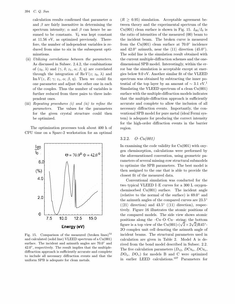
394 C. Q. Sun
calculation results confirmed that parameter α
and β are fairly insensitive in determining the
spectrum intensity; α and β can hence be as-
sumed to be constants. V0 was kept constant
at 11.56 eV, as optimized previously. There-
fore, the number of independent variables is re-
duced from nine to six in the subsequent opti-
mizations.
(ii) Utilizing correlations between the parameters.
As discussed in Subsec. 2.4.2, the combinations
of (z0, λ) and (γ, δ; z1, α; β, η) are correlated
through the integration of ReV (z; z0, λ) and
ImV (z, E; γ; z1, α; β, η). Then we could fix
one parameter and adjust the other one in each
of the couples. Thus the number of variables is
further reduced from three pairs to three inde-
pendent ones.
(iii) Repeating procedures (i) and (ii) to refine the
parameters. The values for the parameters
for the given crystal structure could then
be optimized.
The optimization processes took about 400 h of
CPU time on a Sparc-2 workstation for an optimal
� � � � � � � � � � � � � � ��
� � �
� � �
� � ��
� � � � � � � �
� � � � � � � � � � � ��� � �
� � �
Fig. 15. Comparison of the measured (broken lines)52
and calculated (solid line) VLEED spectrum of a Cu(001)surface. The incident and azimuth angles are 70.0◦ and42.0◦, respectively. The result implies that the multiple-diffraction approach is sufficiently accurate and completeto include all necessary diffraction events and that theuniform SPB is adequate for clean metals.
(R ≥ 0.95) simulation. Acceptable agreement be-
tween theory and the experimental spectrum of the
Cu(001) clean surface is shown in Fig. 15. I00/I0 is
the ratio of intensities of the measured (00) beam to
the incident beam. The broken curve is measured
from the Cu(001) clean surface at 70.0◦ incidence
and 42.0◦ azimuth, near the 〈11〉 direction (45.0◦).
The solid line is the simulation result obtained with
the current multiple-diffraction schemes and the one-
dimensional SPB model. Interestingly, within the er-
ror bar the simulation is acceptable except at ener-
gies below 9.0 eV. Another similar fit of the VLEED
spectrum was obtained by subtracting the inner po-
tential of the top layer by an amount of ∼ 3.1 eV.1
Simulating the VLEED spectrum of a clean Cu(001)
surface with the multiple-diffraction models indicates
that the multiple-diffraction approach is sufficiently
accurate and complete to allow the inclusion of all
necessary diffraction events. Importantly, the con-
ventional SPB model for pure metal (ideal Fermi sys-
tem) is adequate for producing the correct intensity
for the high-order diffraction events in the barrier
region.
3.2.2. O–Cu(001)
In examining the code validity for Cu(001) with oxy-
gen chemisorption, calculations were performed by
the aforementioned convention, using geometric pa-
rameters of several missing-row structural submodels
to optimize the SPB parameters. The best model is
then assigned to the one that is able to provide the
closest fit of the measured data.
Conventional simulation was conducted for the
two typical VLEED I–E curves for a 300 L oxygen-
chemisorbed Cu(001) surface. The incident angle
(relative to the normal of the surface) is 69.0◦ and
the azimuth angles of the compared curves are 23.5◦
(〈21〉 direction) and 43.5◦ (〈11〉 direction), respec-
tively. Figure 16 illustrates the atomic positions of
the compared models. The side view shows atomic
positions along the –Cu–O–Cu– string; the bottom
figure is a top view of the Cu(001)-(√
2× 2√
2)R45◦-
2O complex unit cell denoting the azimuth angle of
incident beams. The structural parameters used in
calculation are given in Table 2. Model A is de-
rived from the bond model described in Subsec. 2.2.
The five calculation parameters (D12, DCux, DCuz,
DOx, DOz) for models B and C were optimized
in earlier LEED calculations.107 Parameters for
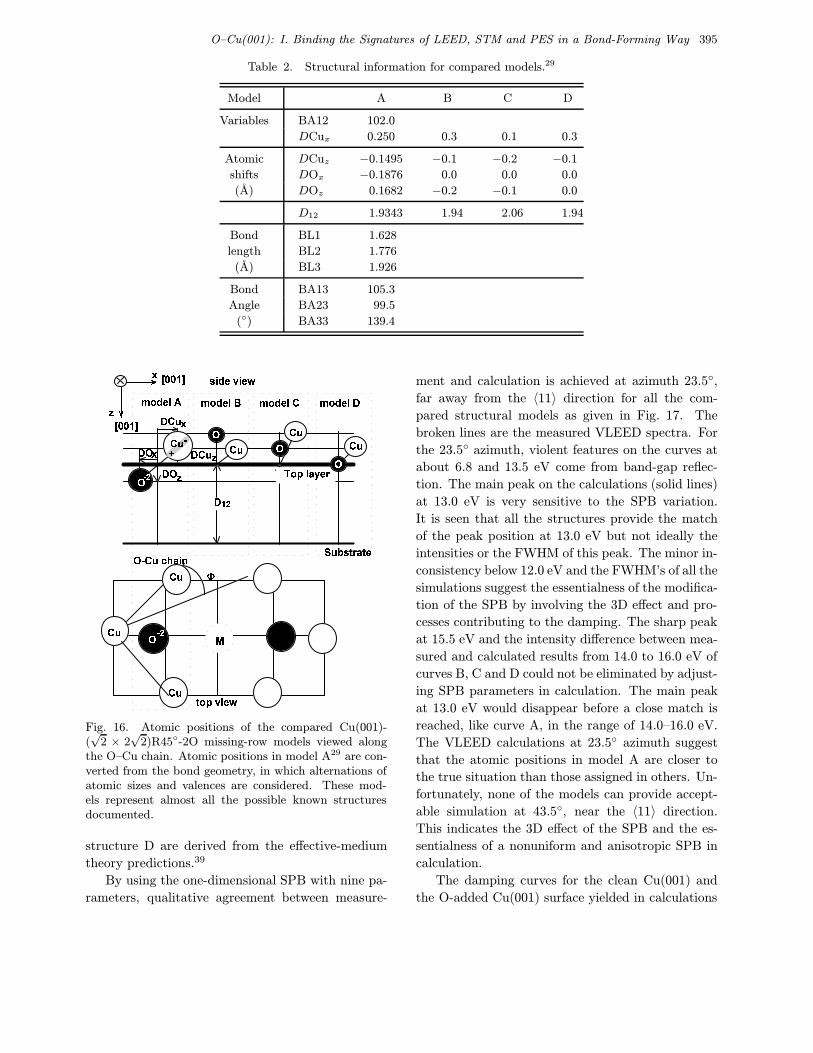
O–Cu(001): I. Binding the Signatures of LEED, STM and PES in a Bond-Forming Way 395
Table 2. Structural information for compared models.29
Model A B C D
Variables BA12 102.0
DCux 0.250 0.3 0.1 0.3
Atomic DCuz −0.1495 −0.1 −0.2 −0.1
shifts DOx −0.1876 0.0 0.0 0.0
(A) DOz 0.1682 −0.2 −0.1 0.0
D12 1.9343 1.94 2.06 1.94
Bond BL1 1.628
length BL2 1.776
(A) BL3 1.926
Bond BA13 105.3
Angle BA23 99.5
(◦) BA33 139.4
� �� �
� �
� � � � � � � � �
� �
� �
� � � � �
� �
� �
�
�
� � � � � � !" # " �# " �
# $ % �
# $ % �
& � ' � ( & � ' � ) & � ' � $ & � ' � #"
""
* + ' , + -
$ %
. ./ 0 1 2 3 4 5 6 7
81 2
1 2
1 2
9 : ; < 6 = >
/ ? @
A
B
Fig. 16. Atomic positions of the compared Cu(001)-(√
2 × 2√
2)R45◦-2O missing-row models viewed alongthe O–Cu chain. Atomic positions in model A29 are con-verted from the bond geometry, in which alternations ofatomic sizes and valences are considered. These mod-els represent almost all the possible known structuresdocumented.
structure D are derived from the effective-medium
theory predictions.39
By using the one-dimensional SPB with nine pa-
rameters, qualitative agreement between measure-
ment and calculation is achieved at azimuth 23.5◦,
far away from the 〈11〉 direction for all the com-
pared structural models as given in Fig. 17. The
broken lines are the measured VLEED spectra. For
the 23.5◦ azimuth, violent features on the curves at
about 6.8 and 13.5 eV come from band-gap reflec-
tion. The main peak on the calculations (solid lines)
at 13.0 eV is very sensitive to the SPB variation.
It is seen that all the structures provide the match
of the peak position at 13.0 eV but not ideally the
intensities or the FWHM of this peak. The minor in-
consistency below 12.0 eV and the FWHM’s of all the
simulations suggest the essentialness of the modifica-
tion of the SPB by involving the 3D effect and pro-
cesses contributing to the damping. The sharp peak
at 15.5 eV and the intensity difference between mea-
sured and calculated results from 14.0 to 16.0 eV of
curves B, C and D could not be eliminated by adjust-
ing SPB parameters in calculation. The main peak
at 13.0 eV would disappear before a close match is
reached, like curve A, in the range of 14.0–16.0 eV.
The VLEED calculations at 23.5◦ azimuth suggest
that the atomic positions in model A are closer to
the true situation than those assigned in others. Un-
fortunately, none of the models can provide accept-
able simulation at 43.5◦, near the 〈11〉 direction.
This indicates the 3D effect of the SPB and the es-
sentialness of a nonuniform and anisotropic SPB in
calculation.
The damping curves for the clean Cu(001) and
the O-added Cu(001) surface yielded in calculations
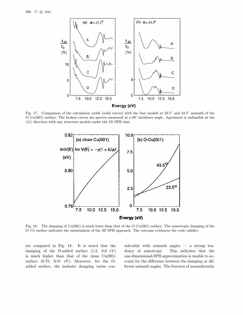
396 C. Q. Sun
�
�
�
�
� � � � � � � � � � � � � �
�
�
� �
� � � �
� � � � � � � � � �
�� � �
�
�
�
!! "
" "
# $ %
&
' () & * ' ) ' * + ) & * & ) '
# , % - . / 0 1 2 3
44 5
5 5
6 7 8
Fig. 17. Comparison of the calculation yields (solid curves) with the four models at 23.5◦ and 43.5◦ azimuth of theO–Cu(001) surface. The broken curves are spectra measured at a 69◦-incidence angle. Agreement is unfeasible at the〈11〉 direction with any structure models under the 1D SPB wise.
Fig. 18. The damping of Cu(001) is much lower than that of the O–Cu(001) surface. The anisotropic damping of theO–Cu surface indicates the essentialness of the 3D SPB approach. The outcome evidences the code validity.
are compared in Fig. 18. It is noted that the
damping of the O-added surface (1.2, 9.0 eV)
is much higher than that of the clean Cu(001)
surface (0.78, 0.81 eV). Moreover, for the O-
added surface, the inelastic damping varies con-
siderably with azimuth angles — a strong ten-
dency of anisotropy. This indicates that the
one-dimensional-SPB approximation is unable to ac-
count for the difference between the damping at dif-
ferent azimuth angles. The features of nonuniformity
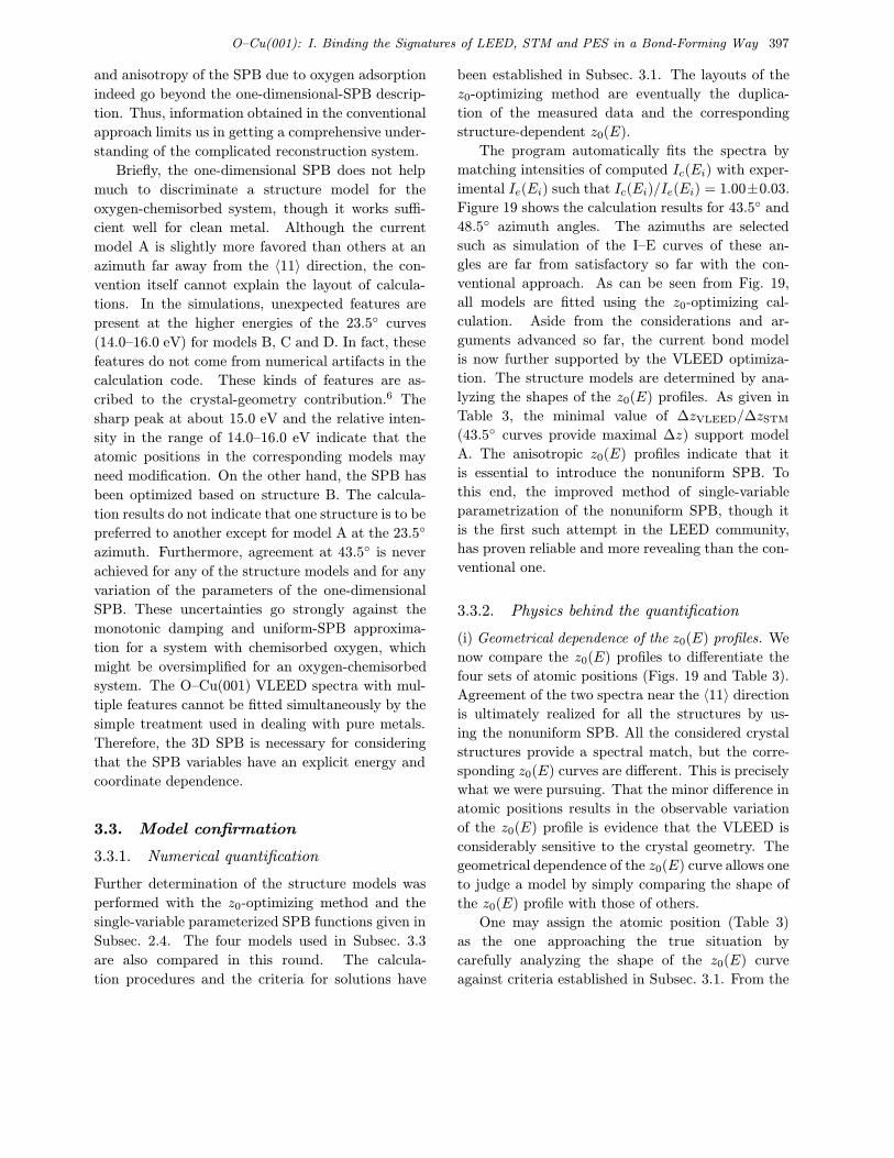
O–Cu(001): I. Binding the Signatures of LEED, STM and PES in a Bond-Forming Way 397
and anisotropy of the SPB due to oxygen adsorption
indeed go beyond the one-dimensional-SPB descrip-
tion. Thus, information obtained in the conventional
approach limits us in getting a comprehensive under-
standing of the complicated reconstruction system.
Briefly, the one-dimensional SPB does not help
much to discriminate a structure model for the
oxygen-chemisorbed system, though it works suffi-
cient well for clean metal. Although the current
model A is slightly more favored than others at an
azimuth far away from the 〈11〉 direction, the con-
vention itself cannot explain the layout of calcula-
tions. In the simulations, unexpected features are
present at the higher energies of the 23.5◦ curves
(14.0–16.0 eV) for models B, C and D. In fact, these
features do not come from numerical artifacts in the
calculation code. These kinds of features are as-
cribed to the crystal-geometry contribution.6 The
sharp peak at about 15.0 eV and the relative inten-
sity in the range of 14.0–16.0 eV indicate that the
atomic positions in the corresponding models may
need modification. On the other hand, the SPB has
been optimized based on structure B. The calcula-
tion results do not indicate that one structure is to be
preferred to another except for model A at the 23.5◦
azimuth. Furthermore, agreement at 43.5◦ is never
achieved for any of the structure models and for any
variation of the parameters of the one-dimensional
SPB. These uncertainties go strongly against the
monotonic damping and uniform-SPB approxima-
tion for a system with chemisorbed oxygen, which
might be oversimplified for an oxygen-chemisorbed
system. The O–Cu(001) VLEED spectra with mul-
tiple features cannot be fitted simultaneously by the
simple treatment used in dealing with pure metals.
Therefore, the 3D SPB is necessary for considering
that the SPB variables have an explicit energy and
coordinate dependence.
3.3. Model confirmation
3.3.1. Numerical quantification
Further determination of the structure models was
performed with the z0-optimizing method and the
single-variable parameterized SPB functions given in
Subsec. 2.4. The four models used in Subsec. 3.3
are also compared in this round. The calcula-
tion procedures and the criteria for solutions have
been established in Subsec. 3.1. The layouts of the
z0-optimizing method are eventually the duplica-
tion of the measured data and the corresponding
structure-dependent z0(E).
The program automatically fits the spectra by
matching intensities of computed Ic(Ei) with exper-
imental Ie(Ei) such that Ic(Ei)/Ie(Ei) = 1.00±0.03.
Figure 19 shows the calculation results for 43.5◦ and
48.5◦ azimuth angles. The azimuths are selected
such as simulation of the I–E curves of these an-
gles are far from satisfactory so far with the con-
ventional approach. As can be seen from Fig. 19,
all models are fitted using the z0-optimizing cal-
culation. Aside from the considerations and ar-
guments advanced so far, the current bond model
is now further supported by the VLEED optimiza-
tion. The structure models are determined by ana-
lyzing the shapes of the z0(E) profiles. As given in
Table 3, the minimal value of ∆zVLEED/∆zSTM
(43.5◦ curves provide maximal ∆z) support model
A. The anisotropic z0(E) profiles indicate that it
is essential to introduce the nonuniform SPB. To
this end, the improved method of single-variable
parametrization of the nonuniform SPB, though it
is the first such attempt in the LEED community,
has proven reliable and more revealing than the con-
ventional one.
3.3.2. Physics behind the quantification
(i) Geometrical dependence of the z0(E) profiles. We
now compare the z0(E) profiles to differentiate the
four sets of atomic positions (Figs. 19 and Table 3).
Agreement of the two spectra near the 〈11〉 direction
is ultimately realized for all the structures by us-
ing the nonuniform SPB. All the considered crystal
structures provide a spectral match, but the corre-
sponding z0(E) curves are different. This is precisely
what we were pursuing. That the minor difference in
atomic positions results in the observable variation
of the z0(E) profile is evidence that the VLEED is
considerably sensitive to the crystal geometry. The
geometrical dependence of the z0(E) curve allows one
to judge a model by simply comparing the shape of
the z0(E) profile with those of others.
One may assign the atomic position (Table 3)
as the one approaching the true situation by
carefully analyzing the shape of the z0(E) curve
against criteria established in Subsec. 3.1. From the
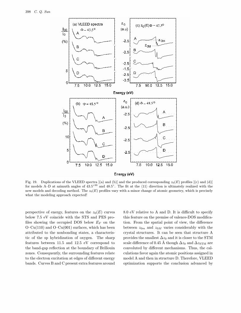
398 C. Q. Sun
������ ��
���
�
�
�
�
�
�
�
�� ��� � ��
� � ���� ���
�
�
�
�
�� ��� � ��
� ��
������
� �
� �
� �
� �
� � ����
�
�
�
�
�
�
�
�� ��� � �� �� ��� � ��
������ ��
�
���
��
�
��
� �
� �
� �
� �
���
��
�� � ���� �����
�
���� � ������ ����� ������� �� � ����
�
��
��
���
�
��
��
���
Fig. 19. Duplications of the VLEED spectra [(a) and (b)] and the produced corresponding z0(E) profiles [(c) and (d)]for models A–D at azimuth angles of 43.5◦99 and 48.5◦. The fit at the 〈11〉 direction is ultimately realized with thenew models and decoding method. The z0(E) profiles vary with a minor change of atomic geometry, which is preciselywhat the modeling approach expected!
perspective of energy, features on the z0(E) curves
below 7.5 eV coincide with the STS and PES pro-
files showing the occupied DOS below EF on the
O–Cu(110) and O–Cu(001) surfaces, which has been
attributed to the nonbonding states, a characteris-
tic of the sp hybridization of oxygen. The sharp
features between 11.5 and 12.5 eV correspond to
the band-gap reflection at the boundary of Brillouin
zones. Consequently, the surrounding features relate
to the electron excitation at edges of different energy
bands. Curves B and C present extra features around
8.0 eV relative to A and D. It is difficult to specify
this feature on the premise of valence-DOS modifica-
tion. From the spatial point of view, the difference
between z0m and z0M varies considerably with the
crystal structures. It can be seen that structure A
provides the smallest ∆z0 and it is closer to the STM
scale difference of 0.45 A though ∆z0 and ∆zSTM are
convoluted by different mechanisms. Thus, the cal-
culations favor again the atomic positions assigned in
model A and then in structure D. Therefore, VLEED
optimization supports the conclusion advanced by

O–Cu(001): I. Binding the Signatures of LEED, STM and PES in a Bond-Forming Way 399
Table 3. Quantitative analysis of the VLEED spectrum at 43.5◦ azimuth for the Cu(001)-(2√
2×√
2)R45◦-2O−2 surface.99,a
Models in E −z0 Intensity Intensity ∆zVLEED
Fig. 19 (eV) (a.u.) (theory) (experiment) (A)∆zVLEED
∆zSTM
A 8.3 2.3861 0.02261 0.02216
12.6 3.3725 0.00454 0.00453 0.5218 1.16
B 8.2 2.2610 0.02214 0.02174
13.0 3.6154 0.00615 0.00553 0.7165 1.59
C 7.9 2.3852 0.02096 0.02070
12.6 3.6760 0.00771 0.00453 0.6828 1.52
D 8.9 2.2230 0.02984 0.02968
12.7 −3.6228 0.00565 0.00440 0.7406 1.65
a∆zSTM = 0.45 A.37 ∆zVLEED = |z0M − z0m| × 0.529 (A). Energies between 11.0 eV and12.0 eV are excluded for the multiple z0 solutions provided. Potential barrier parametersare V0 = 10.50 eV, γ = 0.9703, δ = 4.4478.
Jacobson and Nørskov39 that the oxygen atoms go
underneath the first Cu layer for bonding. At the
same time there is a pairing of Cu dipoles over the
missing row. In fact, as described in Subsec. 3.2,
the pairing dipoles and the missing-row vacancies
originate from the Cu3O2 surface bonding. Unfor-
tunately, normal LEED optimization could hardly
discriminate the difference of models B and C based
on the minimization of the R factor.
(ii) The behavior of surface electrons. The un-
derlying physics of the above results agrees with the
modeling assumptions. These results may deepen
our insight into the behavior of surface electrons
and quantify the localized features of O-added sur-
faces as observed with STM. At the dipole site,
z1∼= z0, α ∼= λ−1. This describes that the
metal dipoles enhance the SPB through the out-
ward shift of the wave function giving a high de-
gree of saturation. For the O–Cu(001) surface, the
z0M [z0M/z0(Cu) = 3.37/2.50 ≈√
2) and the λM[λM/λ(Cu) = 1.27/0.9 ≈
√2] are
√2 times that of
the clean Cu(001) surface. The conductive electrons
colonize and form electron islands (metal dipoles).
The values of z0M and λM also quantify the protru-
sions in the STM image thus: the higher the islands,
the denser the electron cloud. In the missing-row
site, z1 � z0, α� λ−1, i.e. the missing-row vacancy
is not occupied by “free electrons” leading to the
depression in the STM image. On the O–Cu(001)
surface, the lowest saturation degree of the SPB is
[λm/λ(Cu) = 0.65/0.9 ≈] 1/√
2 times that of the
Cu(001) surface. Therefore, the electrons of the O-
chemisorbed surfaces are rather local. It is reason-
able to describe the O–metal surface as a non-Fermi
system that absents freely moving electrons. This
mechanism reveals that the O–Cu(001) surface con-
sists of a dipole layer that lowers the work function
and is also responsible for the nonohmic rectification
of an oxide surface.
As demonstrated, the current nonuniform-SPB
approach is able to account for the behavior of elec-
trons on the Cu surfaces with chemisorbed oxygen.
The formulations can reasonably well quantify the
localized features as revealed by STM and STS. As
an important factor determining the interaction be-
tween incident electrons and the surface, the vari-
ation of the valence DOS can be obtained from
the z0(E) profile. Because the z0(E) profiles vary
with crystal structure, the difficulty of simultane-
ously identifying crystal structure and electronic dis-
tribution has thus been overcome completely with
simplified optimizations. The consistency of the
VLEED profiles z0(E) with STM and STS observa-
tions is evidence that the current SPB is essentially
appropriate.
400 C. Q. Sun
4. Summary
We have thus completed and justified the model for
oxygen adsorption on to the particular Cu(001) sur-
face. An attempt has been made to fit the VLEED
spectra of the O–Cu(001) surface by using various
structural models and different SPB approaches as
well as different decoding skills. Both the conven-
tional and innovative methods consistently support
the current bond model. The conventional SPB
failed to discriminate the structural models with a
minor difference in atomic positions in the symmetric
azimuth, indicating the essentialness of implement-
ing the 3D SPB. The single-variable parametrization
method is able to provide quantitative agreement of
the VLEED spectra at all the azimuth angles with
all the compared models. The geometrically depen-
dent z0(E) profiles enable us to judge the models
upon physical criteria, which is perhaps precisely
what one expected. Quantitative calculations based
on the new models and the new skills have proven
the new premise to be definitive, reliable and more
revealing than the conventional wisdom.
Furnished with the combination of STM, PES
and VLEED, with enhanced capabilities, the model
can formulate the reaction with specification of the
individual atomic valence, surface morphology and
valence-DOS features. The model indicates that ox-
idation is a kinetic process in which O−1 forms first
and then O−2 follows with sp-orbital hybridization
and lone-pair production. O−2 prefers the nearly
central position of a tetrahedron and the surface
atoms move collectively. As a consequence of bond
forming, oxygen derives four additional strongly lo-
calized DOS features in the valence band and above.
These are O–M bonding, nonbonding lone pairs of
oxygen, antibonding metal dipoles and the holes
around EF , in addition to the H-bond-like. There-
fore, oxygen possesses the special capacity to create a
gap or widen the existing band gap, and add an anti-
bonding subband above EF reducing the work func-
tion, which agrees with the PES detection of a num-
ber of metal surfaces with chemisorbed oxygen. The
parametrized SPB functions uncover the full capacity
of VLEED in simultaneously determining the bond
geometry, the shape of the SPB and the variation of
the valence DOS, and their interdependence. One
can judge models by simply comparing the shape
of the geometrically dependent z0(E) curves. The
oxide bond forming and its consequences are respon-
sible for all the observations, whether static or ki-
netic. Atomic dislocation and surface relaxation are
determined by the bond geometry. The strong lo-
calization of surface electrons and variation of the
energy states result from the electron transportation
from one energy level to the other of different atoms
such as polarization and ionization. It is emphasized
that the bonding effect is readily detectable while
the process of electron transportation is beyond the
capacity of currently available means. The overall
approaches not only reflect properly the real process
of reaction but also the natural link among the iden-
tities of STM/S, LEED and PES, in addition to the
reduced numerical efforts and solution certainty.
In the next issue,3 we will report on the nu-
merical justification of the capacity and reliabil-
ity of VLEED, and on using VLEED to quantify
the four-stage O–Cu(001) bond-forming dynamics.
Thus, we have motivated, constructed, justified and
applied the models and the decoding technique to
the particular O–Cu(001) system. Further exten-
sion of the established premise to catalytic electron-
ics and nanosolid is in progress. Another indepen-
dent review108 will be issued elsewhere, focusing on
the O–(Cu, Rh){(001), (110), (111)}, O–(Pd, Ag,
Ni, Pt)(110), O–(Co, Ru){(101 0), (0001)}, and (N,
C)-Ni(001) surface bonding kinetics and technical
applications.
It is understood that formation of the basic ox-
ide tetrahedron, and consequently the bond-forming
kinetics and the oxygen-derived DOS features, is
intrinsically common for all the analyzed systems.
What differ the uncommon patterns of observation
from a surface to another are the specificities of:
(i) the site of the oxygen, (ii) orders of bond for-
mation and (iii) the orientation of the tetrahedron.
The valences of oxygen, the scale and geometry of
the lattice and the electronegativity of the host solid
determine the specificities extrinsically.
Acknowledgments
I am pleased to thank Profs. P. Jennings, S. Thur-
gate, A. Stelbovics and G. Hitchen for providing
me with the VLEED data and the VLEED code,
as well as for their valuable communications, which
made progress possible. I would also like to thank
Profs. S. Y. Tong, A. T. S. Wee, K. P. Loh, C. L. Bai
O–Cu(001): I. Binding the Signatures of LEED, STM and PES in a Bond-Forming Way 401
and E. Jiang for helpful discussions. Finally, critical
reading and kind endorsement of related work linked
to this presentation by Profs. M. Donath, S. Tear,
G. Russell, L. A. Bursill, L. Holland, O. S. Heavens
and A. Mookerjee are gratefully acknowledged.
References
1. S. M. Thurgate and C. Q. Sun, Phys. Rev. B51, 2410(1995).
2. M. A. Van Hove and S. Y. Tong, Surface Crystallog-raphy by LEED (Springer-Verlag, Berlin, 1979).
3. C. Q. Sun, “O–Cu(001): II. VLEED quantification ofthe Cu3O2 four-stage bond-forming kinetics,” Surf.Rev. Lett., to be published.
4. J. B. Pendry, Low Energy Electron Diffraction: TheTheory and Its Application to the Determination ofSurface Structure (Academic, London, 1974).
5. E. G. McRae, Surf. Sci. 11, 492 (1968).6. R. O. Jones and P. J. Jennings, Surf. Sci. Rep. 9,
165 (1988).7. S. M. Thurgate, G. Hitchen and C. Q. Sun, in Surface
Science, Principles and Applications, eds. R. J. Mac-Donald, E. C. Taglauer and K. R. Wandelt (Springer,1996), p. 29.
8. R. Feder, P. J. Jennings and R. O. Jones, Surf. Sci.61, 307 (1976).
9. L. R. Bedell and H. E. Farnsworth, Surf. Sci. 41, 165(1973).
10. R. C. Jacklevic and L. C. Davis, Phys. Rev. B26,5391 (1982).
11. P. J. Møller, S. A. Komolov and E. F. Lazneva, Surf.Sci. 307 309, 1177 (1994).
12. V. N. Strocov, Solid State Commun. 106, 101 (1998).13. V. N. Strocov, H. I. Starnberg, P. O. Nilsson, H. E.
Brauer, L. J. Holleboom, Phys. Rev. Lett. 79, 467(1997).
14. E. G. McRae and C. W. Caldwell, Surf. Sci. 57, 766(1976).
15. H. Pfnur, M. Lindroos and D. Menzel, Surf. Sci. 248,1 (9991).
16. E. G. McRae, Rev. Mod. Phys. 51, 541 (1979).17. M. A. Van Hove, W. H. Weinberg and C.-M. Chan,
Low-energy Electron Diffraction: Experiment The-ory and Surface Structural Determination (Springer-Verlag, Berlin, 1986).
18. S. Papadia, M. Persson and L. A. Salmi, Phys. Rev.B41, 10237 (1990).
19. G. Hitchen and S. Thurgate, Phys. Rev. B38, 8668(1988).
20. G. Hitchen and S. Thurgate, Surf. Sci. 197, 24(1988).
21. M. Lindroos, H. Pfnur and D. Menzel, Phys. Rev.B33, 6684 (1986).
22. J. M. Baribeau, J. D. Carette, P. J. Jennings, R. O.Jones, Phys. Rev. B32, 6131 (1985).
23. E. Tamura and R. Feder, Solid State Commun. 58,729 (1986).
24. H.-J. Herlt, R. Feder, G. Meister and E. Bauer, SolidState Commun. 38, 973 (1981).
25. S. A. Komolov, Total Current Spectroscopy ofSurfaces (Gordon & Breach, New York, 1992).
26. I. Bartos, P. Jaros, A. Barbieri, M. A. Van Hove,W. F. Chung, Q. Cai and M. S. Altman, Surf. Rev.Lett. 2, 477 (1995).
27. S. M. Thurgate, PhD thesis, “The structure ofthe metal–vacuum interface of copper and nickel,”(Murdoch University Press, Australia, 1982).
28. M. A. Van Hove, J. Cerda, P. Sautet, M. L. Bocquetand M. Salmeron, Prog. Surf. Sci. 54, 315 (1997).
29. C. Q. Sun and C. L. Bai, J. Phys. Chem. Solids 58,903 (1997).
30. F. W. Young, J. V. Cathcart and A. T. Gwathmey,Acta Met. 4, 45 (1956).
31. D. P. Woodruff and T. A. Delchar, Mod. Techniquesof Surface Science (Cambridge University Press,1986).
32. P. S. Bagus and F. Illas, Phys. Rev. B42, 10852(1990).
33. J. K. Nørskov, Surf. Sci. 299/300, 690 (1994).34. H. C. Zeng, R. A. McFarlane, R. N. S. Sodhi and
K. A. R. Mitchell, Can. J. Chem. 66, 2054 (1988).35. T. Lederer, D. Arvanitis, G. Comelli, L. Troger and
K. Baberschke, Phys. Rev. B48, 15390 (1993).36. T. Fujita, Y. Okawa, Y. Matsumoto and K. Tanaka,
Phys. Rev. B54, 2167 (1996).37. F. Jensen, F. Besenbacher, E. Lagsgaard and I.
Stensgaard, Phys. Rev. B42, 9206 (1990).38. F. Besenbacher and J. K. Nørskov, Prog. Surf. Sci.
44, 5 (1993).39. K. W. Jacobsen and J. K. Nørskov, Phys. Rev. Lett.
65, 1788 (1990).40. D. Arvanitis, G. Comelli, T. Lederer, H. Rabus and
K. Baberschke, Chem. Phys. Lett. 211, 53 (1993).41. T. Yokoyama, D. Arvanitis, T. Lederer, M. Tischer,
L. Troger, K. Baberschke and G. Comelli, Phys. Rev.B48, 15405 (1993).
42. K.-I. Tanaka, T. Fujita and Y. Okawa, Surf. Sci. 401,L407 (1998).
43. G. Hitchen, S. M. Thurgate and P. Jennings, Aust.J. Phys. 43, 519 (1990).
44. S. Warren, W. R. Flavell, A. G. Thomas, J. Holling-worth, P. L. Wincott, A. F. Prime, S. Downes andC. J. Chen, Phys. Cond. Matt. 11, 5021 (1999).
45. V. P. Belash, I. N. Klimova, V. I. Kormilets, V. Y.Trubjtsjn and L. D. Fjnkelstein, Surf. Rev. Lett. 6,383 (1999).
46. V. Dose, Surf. Sci. Rep. 5, 337 (1986).47. S. Hufner, Photoelectron Spectroscopy: Principles
and Applications (Springer-verlag, 1995), p. 339.48. W. Jacob, V. Dose and A. Goldmann, Appl. Phys.
A41, 145 (1986).49. V. A. Bondzie, P. Kleban and D. J. Dwyer, Surf. Sci.
347, 319 (1996).
402 C. Q. Sun
50. C. Q. Sun and S. Li, Surf. Rev. Lett. 7, L213 (2000).51. R. O. Jones and P. J. Jennings, Phys. Rev. B27, 4702
(1983).52. G. J. Hitchen, S. M. Thurgate and P. Jennings, Phys.
Rev. B44, 3939 (1991).53. G. Malmstrom and J. Rundgren, Comput. Phys.
Commun. 19, 263 (1980).54. C. L. Bai, Scanning Tunneling Microscopy and Its
Applications, Springer Series in Surf. Sci., Vol. 32(Springer-Verlag, Berlin, 1995), pp. 34–37, 183, 222.
55. J. Wintterlin and R. J. Behm, in Scanning Tunnel-ing Microscopy I, Chap. 4, eds. H. J. Gunthert andR. Wiesendanger (Springer-Verlag, Berlin, 1992).
56. H. H. Rotermund, Surf. Sci. 283, 87 (1993).57. U. Dobler, K. Baberschke, J. Stohr and D. A. Outka,
Phys. Rev. B31, 2532 (1985).58. G. Ertl, Surf. Sci. 299/230, 742 (1994).59. N. D. Lang, Phys. Rev. Lett. 55, 230 (1985).60. G. Ertl and T. N. Rhodin, The Nature of Surface
Chemical Bond (North-Holland, 1979).61. M. A. Van Hove and G. A. Somorjai, Surf. Sci.
299 230, 487 (1994).62. L. Pauling, The Nature of the Chemical Bond
(Cornell University Press 1939; 3rd ed., New York,1960).
63. C. Q. Sun, Mod. Phys. Lett. B12, 849 (1998).64. C. W. Keenan, D. C. Kleinfelter and J. H. Wood,
General College Chemistry, 6th ed. (Harper & Row,1979).
65. V. M. Goldschmidt, Ber. Deut. Chem. Ges. 60, 1270(1927).
66. L. Pauling, J. Am. Chem. Soc. 69, 542 (1947).67. M. J. Sinnott, The Solid State for Engineers (John
Wiley & Sons, New York, 1963).68. J. D. Jorgensen, Phys. Today 44, 34 (1991).69. H. Kamimura, E. M. Matsuno and H. Ushio, Com.
Cond. Matt. Phys. 15, 273 (1992).70. P. J. Jennings, in Surface Analysis Methods in Mate-
rials Science, eds. D. J. O’Connor, B. A. Sexton andR. C. Smart (Springer-Verlag, Berlin, 1992).
71. D. L. Adams, H. B. Nielsen, J. N. Andersen, I. Stens-gaard, R. Feidenhans’l and J. E. Sørensen, Phys. Rev.Lett. 49, 669 (1982).
72. Y. Kuk, F. M. Chua, P. J. Silverman and J. A. Meyer,Phys. Rev. B41, 12393 (1990).
73. C. Q. Sun, J. Phys. Cond. Matt. 11, 4801 (1999).74. H. Huang, C. Q. Sun and P. Hing, J. Phys. Cond.
Matt. 12, L127 (2000).75. C. Q. Sun, X. W. Sun, H. Q. Gong, H. Huang, H. Ye,
D. Jin and P. J. Hing, Phys. Cond. Matt. 11, L547(1999).
76. H. Huang, C. Q. Sun, T. S. Zhang, H. Ye andP. Hing, Phys. Rev. B, in press.
77. H. T. Ye, C. Q. Sun and P. Hing, J. Appl. Phys. D33,L148 (2000).
78. C. Q. Sun, B. K. Tay, S. P. Lau and X. W. Sun, SPIEProc. 4228, 302 (2000).
79. N. D. Lang, Phys. Rev. B37, 10395 (1988).80. A. Beiser, Perspective of Modern Physics, 18th ed.
(McGraw-Hill, Singapore, 1988).81. C. Q. Sun, Mod. Phys. Lett. B11, 1115 (1997).82. C. Q. Sun, Surf. Rev. Lett. 5, 465 (1998).83. C. Q. Sun, Int. J. Mod. Phys. B12, 951 (1998).84. A. P. Cole, D. E. Root, P. Mukherjee, E. I. Soloman
and T. D. P. Stack, Science 273, 1848 (1996).85. M. C. Asensio, M. J. Ashwin, A. L. D. Kilcoyne, D. P.
Woodruff, A. W. Robinson, T. Lindner, J. S. Somer,D. E. Ricken and A. M. Bradshaw, Surf. Sci. 236, 1(1990).
86. F. M. Chua, Y. Kuk and P. J. Silverman, Phys. Rev.Lett. 63, 386 (1989).
87. S. R. Morrison, The Chemical Physics of Surfaces(Plenum, New York and London, 1977).
88. C. Q. Sun, Appl. Phys. Lett. 72, 1706 (1998).89. H. H. Rotermund, J. Lauterbach and G. Haas, Appl.
Phys. A: Solids and Surfaces 57, 507 (1993).90. J. Lauterbach and H. H. Rotermund, Surf. Sci. 311,
231 (1994).91. J. C. Boulliard and M. P. J. Sotto, Cryst. Growth
110, 878 (1991).92. R. E. Dietz, E. G. McRae and R. L. Campbell, Phys.
Rev. Lett. 45, 1280 (1980).93. R. O. Jones, P. J. Jennings and O. Jepsen, Phys. Rev.
B29, 6474 (1984).94. A. Adnot and J. D. Carette, Phys. Rev. Lett. 38,
1084 (1977).95. M. N. Read and A. S. Christopoulos, Phys. Rev.
B37, 10407 (1988).96. J. E. Demuth, P. M. Marcus and D. W. Jepsen, Phys.
Rev. B11, 1460 (1975).97. P. Jennings, private commun. (Murdoch, Australia,
1994).98. M. Nishijima, Solid State Commun. 58, 75 (1986).99. C. Q. Sun and C. L. Bai, J. Phys. Cond. Matt. 9,
5823 (1997).100. C. Q. Sun, Vacuum 48, 491 (1997).101. C. Q. Sun, PhD thesis, “Modeling of bond struc-
ture and potential barrier of the O–Cu(100) surfacecharacterized by STM/S & VLEED,” (MurdochUniversity Press, 1995).
102. C. Q. Sun and C. L. Bai, Mod. Phys. Lett. B11, 201(1997).
103. G. Hitchen, private commun. (Murdoch University,Australia, 1994).
104. P. J. Jennings and S. M. Thurgate, Surf. Sci. 104,L210 (1981).
105. S. M. Thurgate, private commun. (Murdoch Univer-sity, Australia, 1992).
106. H. C. Zeng and K. A. R. Mitchell, Surf. Sci. 239,L571 (1990).
107. A. Atrei, U. Bardi, G. Rovida, E. Zanazzi andG. Casalone, Vacuum 41, 333 (1990).
108. C. Q. Sun, “Oxidation electronics,” to be published.