OASIS: An Online and Accurate Technique for Local-alignmentSearches on Biological Sequences

Colin Meek Jignesh M. PatelDepartment of Electrical Engineering and Computer Science

The University of Michigan, Ann Arbor, MI 48109, USA�meek, jignesh�@eecs.umich.edu

Abstract

The analysis of sequence data is central in the increasingly important area of functional proteomics and

genomics. A common type of query that is posed by scientists in these areas is to take an input query sequence

and search against a large protein or gene data set finding targets that match the input query sequence. Such

queries are commonly evaluated using local-alignment algorithms to find approximate matches. The current

set of search tools used for this purpose employ heuristics to improve the speed of the search. However,

such heuristics can sometimes miss out matching targets. Given the high-stakes involved in these biological

research projects, it is natural to wonder if an algorithm could be designed that is guaranteed not to miss any

results given the query specification.

There are a few know algorithms for identifying all local alignments, but so far these have been considered

to be too computationally intensive to be used for searching large biological sequences. The most popular of

these accurate search algorithms is the Smith-Waterman algorithm. In this paper, we take on the challenge of

designing an accurate and efficient algorithm for evaluating local-alignment searches against large biological

data sets. We propose a novel algorithm called OASIS that uses an A*-style search algorithm, which is

driven by a suffix tree index built on the input data set. We experimentally evaluate the proposed algorithm

using a number of motif queries against the entire Swiss Protein data set. We demonstrate that OASIS is an

order-of-magnitude faster than the Smith-Waterman algorithm in most cases. Consequently, we believe that

it may now be possible to use accurate search tools for evaluating local-alignments against actual biological

data sets. Finally, OASIS also has the nice property of returning target sequences in the order of the matching

score, which allows its use in an online setting in which the user can abort a query after viewing partial

results.

1

1 Introduction

In the new and emerging area of functional genomics and proteomics life science researchers often have to

query biological sequences. Frequently, the scientist has a protein or nucleotide sequence and they want to

check if this sequence has been seen before, or postulate the function of a sequence based on similarities to

known sequences. While there are various ways of finding matching sequences, local alignment is frequently

used: using some scoring metric for alignments, we can determine the likelihood that two sequences are related.

In the late 1980s when computer scientists started investigating algorithms for fast local alignment, it was too

expensive to answer local alignment queries by matching the query sequence against each sequence in the

database. However, a lot has changed since that time. Marching in line with Moore’s law, processors have

continued an exponential increase in computational speed, and main memory has become quite inexpensive. As

a result, it is now reasonable to expect that scientists have, or will soon have GHz processor machines on their

desktops with a GB or more of main memory.

A popular tool for local sequence alignment, BLAST [1], performs a linear search for strong local alignments

using discrete finite automata (DFA). The DFA is designed to accept q-grams within a certain edit distance from

query subsequences, with the restriction that insertions and deletions are disallowed [15]. All accepted q-grams

are extended to the left and the right to determine whether they meet the search criteria, using some ceiling on the

probability that such a match would occur by chance. This heuristic filter has been shown to result in very few

false negatives, but does not have 100% precision and recall. Given the high-stakes and cost involved in many

life sciences experiment, such as drug discovery or gaining a better understanding of the causes of a disease, it

is natural to wonder if it is possible to design a fast and accurate algorithm for local sequence alignment that is

guaranteed to not miss any answers.

While a number of refinements of the BLAST algorithm have been proposed and continue to be proposed,

these techniques focus on improving the speed of the basic BLAST algorithm. In this paper, we take a novel

approach to this problem. We recognize that with current hardware configurations large main-memory config-

urations are common. We design an algorithm called OASIS (an Online and Accurate Search technique for

Inferring local-alignments on Sequences) for fast and accurate local alignment searches on sequences.

OASIS is designed to accurately evaluate local-alignment matches over multiple sequences. Employing a

best-first search, it identifies alignments in score order, making it ideal for online results generation. A suffix

tree that is built on the data set enables a sub-linear scan for potential targets, by simply “walking” down the

tree. We directly identify maximum score local alignments, using a best-first (A*) suffix tree traversal guided by

2

intermediate results that are produced by using the Smith-Waterman (S-W) dynamic programming approach [19]

to compute string edit distances between the input query and suffixes of the data set[19].

The most space efficient suffix trees have a space utilization of roughly 12.5 bytes per base pair (bp) [14].

Given a query of length �, and a database containing sequences with a sum length of �, suffix trees allow for

the identification of exact matches in ���� time. When approximate matches are allowed, the performance

can degrade to ������ time, although we will demonstrate that this upper-bound is too liberal for extremely

large databases! The other accurate local-alignment algorithm (S-W) runs in ����� time under all conditions.

Our algorithm scales fairly well to approximate queries, but its performance nonetheless degrades with respect

to S-W as queries become less specific, and query lengths increase. However, a large class of queries that are

posed by scientist involve short query sequences. For example, queries against protein data sets using peptide

motifs as query sequences is frequently used to find proteins that match specific peptides that are observed in an

experiment. Such peptide motifs are much shorter in length than the actual protein, and are commonly used in

querying biological data sets [8]. OASIS is especially suitable for such cases, as is demonstrated in this paper.

Traditionally, the use of suffix trees has been written-off primarily because suffix trees are hard to represent

efficiently on disk, and consequently on large data sets, the performance of algorithms using suffix trees is very

poor. However, we argue that for querying on biological sequences current trends in hardware will allow a large

portion of the suffix tree nodes to be resident in main-memory. We back up our claims by actual experiments

on an actual complete data set (the popular Swiss Protein data set) on a machine that was priced less that $3K a

year ago.

An astute reader may point out that in the last few years the size of the biological sequence data has been

doubling every sixteen months. Processor speeds and memory sizes are keeping up with this doubling of data

set sizes, and unlike Moore’s law it is unclear if this doubling of data sizes is likely to continue for a prolonged

period of time (much of the increase in the data sizes in recent years have come from the public agencies

doing a better job of integrating data from multiple sources). Furthermore, the OASIS algorithm is very easy to

parallelize, and can easily be run on clusters of (cheap) PCs. While we don’t explore parallelism in this paper, it

is our plan to explore this in the future.

The remainder of this paper is organized as follows: we will begin by describing some existing work in this

area, describe the bases for the OASIS algorithm, outline our strategy for the construction and representation of

the underlying index structure in secondary memory, describe the algorithm itself, and finally present results of

experiments on a complete protein database.

3

2 Related Work

We now review some existing work in this area. An effective (but non-accurate) system is QUASAR [4]. Based

on suffix arrays, it achieves a performance gain over BLAST in searches for “strongly similar DNA sequences”

by filtering out sections of the database not likely to generate any useful matches. [6] and [3] have applied suffix

trees to the problem of searching unstructured sequence data, in both cases with reference to genetic sequences.

To our knowledge, no study of the tradeoff point between linear and suffix tree searches has been conducted,

with respect to approximate matching. Approximate matching is a critical component of sequence analysis [7],

so while suffix trees have been proven to be extremely efficient for exact matching, their performance does

degrade when closeness requirements are relaxed. This follows from the intuition that approximate matching

requires branching in the search space.

Trees provide the greatest benefit for hierarchically organized searches. In the case of approximate string

matching, there is no direct hierarchy in the sense that we cannot simply descend the tree to an answer. The

degree of branching in the search for matches increases as we allow for larger edit distance between the query

and the target. At some point, the overhead (space and time) of the tree structure negates the advantage of a hi-

erarchically organized search. Similar problems have been addressed for multi-dimensional indexing, where the

tree structure gracefully incorporates linear storage and search techniques as the data requires it [2], but there is

no clear extension to the string edit-distance domain: searching a hyper-rectangle would result in too many false

hits, and restricts us to a single q value, without the possibility of insertions and deletions. It is possible to index

a 4-gram “TACG” if we map it to a coordinate in 4-d space, � T,A,C,G �. Allowing for insertions and deletions,

we would need to search using hyper-rectangles corresponding to various interpretations of dimensionality, since

insertions and deletions would effectively expand and collapse dimensions in the search space.

3 Local Alignment

Given two sequences of symbols � � ��������� and � � ���������, a local alignment is some way of “lining

up” any two sub-sequences of � and � (for an example, see Figure 1). We will use this notation throughout. �

is an �-length query, where �� is the �� symbol. Similarly, � is an �-length target, where �� is the �� symbol.

In our complexity analyses, � and � will always have this meaning.

There are several alignment operations:

� Replacement with either the same symbol (see label 1 in Figure 1) or a different symbol (see label 2 in

4

C A B I N

D R A I N

- -

& &

&&

Target:

Query:

1 112

3

4

Figure 1: Local alignment example

Figure 1).

� Deletion allows us to skip a symbol in the target (see label 3 in Figure 1).

� Insertion allows us to skip a symbol in the query (see label 4 Figure 1).

Alignments are given scores based on the sum of the scores of each operation involved in the alignment.

Every operation is generalized to a replacement of � � �, where insertions are represented as � � � and

deletions as � � �. The score of an operation is denoted �� � ��. An edit matrix (see Table 1) stores the

scores, so the cost of an operation � � � is simply ��. The Smith-Waterman algorithm [19] finds the local

alignment between two sequences with the maximum possible score using a dynamic programming approach

that runs in ����� time.

A C G T -A 1 -1 -1 -1 -1C -1 1 -1 -1 -1G -1 -1 1 -1 -1T -1 -1 -1 1 -1- -1 -1 -1 -1 -

Table 1: “Unit” edit distance table

3.1 Smith-Waterman Algorithm

This algorithm generates an � by � matrix �, where each entry ���� stores the score of the maximum alignment

between a query (�) and target (� ) ending at �� and �� . Note that we can induce that best possible score from

5

previous entries in the matrix:

���� � ���

�������������������

� �����������������������������������

�������� ���� � ��� �����������

������ ���� � �� ��������

������ ���� ��� �������

�������������������

(1)

The cost of the algorithm is the cost of building the matrix �, which has � �� entries. Consider for example

a query � � “TACG” against a target � � “AGTACGCCTAG”. Table 2 outlines the execution of S-W, using the

edit matrix in Table 1, where � indicates that a replacement yielded the maximum score, � indicates deletion,

and indicates insertion. The bold score entry indicates the maximum score alignment. By backtracking using

the bold arrows, we can uncover the alignment:

� ... T A C G ...

� T A C G

4 Generalized Suffix Tree Structure

In this section, we now outline the basics of the suffix tree, the basic data structure of the OASIS algorithm.

Suffix trees are a special case of �� trees. These are, essentially, trees in which the edges are labeled with

strings from �����, where � is a finite alphabet. Each node can have only one outgoing edge labeled with

�� where � �, which means the branching degree of the tree is at most ���, the cardinality of the symbol

alphabet. The path to a node is described by the concatenation of the strings labeling the edges traversed. For

instance, in Figure 2 ��� ���� � “AG”.

A string � is said to be a word of an �� tree if there exists a node ! such that ��� �!� � “wu”. A suffix tree

� on a string � is an �� tree in which every subsequence of � is a word of � . One final definition is required:

a ������� suffix tree is one in which every node is either the root, a branching node or a leaf. In practice, this

A G T A C G C C T A G

T 0 0 �1 �0 0 0 0 0 �1 �0 0A �1 �0 0 �2 �1 �0 0 0 0 �2 �1C 0 �0 0 1 �3 �2 �1 �1 �0 1 �0G 0 0 0 0 �0 �4 �3 �2 �1 0 �2

Table 2: � matrix built using S-W

6

0A

1A

2A

4A

3A

5A

3L

0L

9L

1L

5L

10L

2L

8L

4L

6L

7Lsymbol

headPos 0

A

1

G

2

T

3

A

4

C

5

G

6

C

7

C

8

T

9

A

10

G

11

$

A

GTACGCCTAG$

$CGCCTAG$

G TACGCC

TAG$

CCTAG$

$TA

CGCCTAG$

G$C

GCCTAG$

CTAG$TAG$

Figure 2: Suffix tree on the sequence “AGTACGCCTAG”

means that all nodes with only one successor are collapsed into their parents, creating multi-symbol arcs. The

tree in Figure 2 is an example of a compact suffix tree. Note that in general, sequences are appended with a

terminal symbol, e.g. $.

4.1 Finding exact matches in a suffix tree

Given a query � � ���������, it is straightforward to confirm its presence in a sequence � represented in a

suffix tree. It is simply a matter of tracing a path, defined by the query, from the root of the tree until either the

query is consumed, or no match is possible, since the tree must contain a path beginning with all subsequences.

If the query is consumed, this means that a match has been found. Consider the query “TACG” posed against

the structure in Figure 2: starting from the root, we can match the first two symbols along the arc 4A, and the

subsequent two symbols on the arc 2L. This indicates that a match exists beginning at position 2 in � (more on

the naming conventions for nodes later in this paper.) In general, once a match has been found, its location(s) in

the target sequence can be identified by descending to its successor leaf/leaves.

4.2 Tree Construction and Representation

In general, the construction and traversal of suffix trees results in “random-like access” [9]. Efficient in-memory

construction methods [16, 20] do not adapt well to secondary-memory [3, 12]. An existing secondary-memory

7

construction technique [12] constructs sub-trees stemming from fixed-length prefixes of each suffix in memory,

by making one pass through the sequence data for each subtree. [3] supports multiple sequences by building trees

for each in memory, and then merging them. Another trie storage method, developed initially for PATRICIA

tries [17] is the “index fabric” [5, 6]. It provides excellent scalability and access patterns, but is optimized for

XML data, and may not effectively handle the redundancy of suffix representations.

We also construct our trees in multiple passes, but use a hashing function over sequence q-grams to determine

which branches of the tree are built in each pass. We use a hash function with � bins, where � is the number of

passes that we will make over the input data set. In each pass, we determine from the first � symbols of every

suffix whether that suffix is to be written in the current pass. In this way we avoid swapping to disc by storing

only the relevant tree branches in memory for each pass. In practice, accessing a suffix tree results in many

random accesses accesses. To minimize this phenomenon, we then reorganize the tree on disk such that siblings

are stored contiguously, since OASIS must explore all children of a node when the node is expanded.

The strings labeling the arcs of a tree are generally referred to indirectly using pointers to the original

sequence. To reduce the number of random accesses incurred by these pointer fetches, we store some of this

data with the actual node: as many symbols as can be stored in 4 bytes using Huffman coding to conserve space

[18]. We need only fetch from the original sequence when the relevant symbols are not stored along with the

node.

4.3 Multi-sequence

A fairly trivial modification of the structure allows for the storage of multiple sequences: we can simply con-

catenate multiple sequences, separated by the terminal symbol. Note that in practice, a match is associated with

the position in the full concatenated sequence, based on the position in the leaf array. We simply store the off-

sets of each sequence, and based on the position, identify the target sequence using a weighted binary search

through the offset table. This tends to work well in practice, since the lengths of individual sequences is fairly

consistent. For instance, given a structure storing " sequences and a position �, with � equal to the sum length

of the sequences, we start the search at sequence �� � "#��, refining the range for the search as we go.

5 �� Heuristic Search

We will now offer a brief overview of �� search, a key aspect of our approach. �� is a technique for bounding

and directing branching searches, a “best-first” strategy wherein nodes showing the greatest promise are ex-

8

panded first. In this instance, we are interested in maximizing score. Each node has associated with it a current

score, and an expected score. At each stage in the search, the node with the highest expected score is expanded.

5.1 Expected Score

In the search, each node � has some score associated with its path from the root, denoted ����. In addition,

we can in many cases make heuristic predictions about the value of the best possible path from that node to the

goal, denoted ���. should be an optimistic heuristic, in the sense that it should never underestimate the actual

best value. The expected value of a node is then simply $��� � ���� ���. Our heuristic is an example of a

monotonic heuristic, which means that the $ -value can never increase, only decrease. Note also that at the goal

state, $��� � ����, since at this point completely accurate predictions are of course available!

5.2 The Algorithm

The successors of the root are first pushed onto a priority-queue, where the ordering is according to $ -value. At

every step, the node with the highest rank is expanded, and its successor pushed on the queue. Based on the

monotonicity assumption, we know that if a goal node is at the top of the queue, no other solution can ever have

a higher $ value. Extending the process, we can identify in order of score the best all goal states.

a:

b: c:

d: e: f:

g: h:

g h 0 10

2 8 1 9

4 0 5 3 8 2

6 0 9 0

Figure 3: Sample search tree for �� search, leaves are goal nodes

Consider the search tree in Figure 3, where the goal states are the leaf states. The algorithm trace is as

follows, where goal states are shown in bold:

9

Step Current Node Q (node/$ -value) Results1 a �b/10,c/10� ��2 b �c/10,e/8,d/4� ��3 c �f/10,e/8,d/4� ��4 f �h/9,e/8,d/4� ��5 h �e/8, d/4� �h�6 e �g/6, d/4� �h�7 g �d/4� �h, g�8 d �� �h, g, d�

Note that in case of ties, as in step 1, we give higher priority to the node with the higher �-value, since we

have less confidence in the -values.

6 OASIS

The basic idea of the algorithm is to perform an �� search, where the search space is defined by a suffix tree,

and nodes are expanded in a manner closely related to S-W. We will begin by describing the specifications for

the algorithm, then describe its operation, and finally give a brief example to demonstrate its execution.

6.1 Specifications

6.1.1 Input

The algorithm takes as input a suffix tree � ���, where � is the concatenation of the sequences ��������.

A query � is given, along with an edit score matrix . �� ���� is the minimum relevant score, to allow

for search pruning, and since such restrictions are useful in practice, to avoid the reporting of trivial align-

ments. ��"���%�� is the maximum number of alignments to return, where only one alignment is returned per

sequence, as with S-W.

6.1.2 Output

The algorithm returns the starting points and scores of each alignment (i.e. the starting point of the word in �

yielding the alignment.) The algorithm operates on-line: as matches are found, they are output in descending

order of alignment score.

6.2 The Algorithm

For expositional purposes, we will describe the algorithm as it relates to ��:

10

6.2.1 �-values

As we follow a path through the suffix tree, we essentially fill in the columns of the S-W matrix, �, with some

key differences. This highlights one advantage of this approach: work can be shared among multiple paths with

the same prefix. We do not however allow for the score to be reset to 0, because this work will be duplicated

elsewhere: resetting to 0 means considering a different starting alignment with respect to �, when all such

alignments are considered along some path in � ���. The �-value associated with a particular node is simply

the maximum value in the last filled-in column of �. In practice, we maintain only this last column along with

the node.

To save time and space, we only expand and store the portions of that column with strictly positive values,

with the exception of the root node, where all values are initialized to zero. We call this alignment pruning.

Again, we do this to avoid duplicating work, since equivalent or better scoring paths can be identified starting

after these alignments through other paths. Essentially, this mirrors the “starting over” process used by S-W. For

instance, consider a partial local alignment between a portion of a query ����������� and the suffix �����������. If

the maximum alignment score beginning at �� � �� and ending at �� � �� is negative, then we can guarantee that

the score of any alignment between ������� ��� and ���������� will have a lower score than the alignment between

������� and �������. We explicitly consider all starting alignments for the query in the column expansion, and

because of the fundamental properties of the suffix tree, we consider all starting alignments, since every suffix

of the database exists along some rooted path through the tree.

6.2.2 - and $ -values

We generate an � �-length vector & , where &� (� � � �) represents the maximum possible alignment

score of ������������� with any arbitrary target, again where the query � � ���������. Calculating these values

is trivial, assuming non-positive values for insertions and deletions. &� is set to zero, since the relevant portion

of the query is null. We can then inductively calculate the remaining values inductively: &��� � &� the

maximum score for the replacement of ����.

Returning to our earlier example, � � “TACG” and the edit matrix in Table 1, each symbol is optimally

replaced by itself, yielding a score of 1, and we have & � ��' ' �' �' ��. This matrix gives an upper limit on

how much the remainder of the query can contribute to the score. Consider the � matrix in Table 2. If we take

the fourth column (under the symbol A), and add the values in the & vector, we get:

11

� & ( � �&

- 4 -0 3 32 2 41 1 20 0 0

Note that the second row predicts the maximum possible (and actual) alignment score extending from ��

and ��, equal to 4. The expected score $ of a node is the maximum ( value associated again with the last

filled column, with the caveat that we do not consider $ -values of pruned alignments. If this $ -value is below

�� ����, the entire node can immediately be pruned (node pruning).

6.2.3 Goal state

Defining the goal state is not straightforward. Clearly leaf nodes are candidates, and are tagged as accepted

if they are not pruned. There is another important case however: if the maximum expected score ever drops

below or equal to the maximum actual score seen anywhere along the ancestor path, then a node is also marked

as accepted. This is because such paths can, by an optimistic heuristic, never yield a stronger alignment than

the one already found. It is advantageous to identify such situations as early as possible so that costly node

expansions can be avoided. Accepted nodes are pushed onto the priority queue, with their expected scores set

equal to the maximum score seen along the path. Accepted states are effectively goal states, in the conventional

language of �� search, since they describe the maximum alignment score along a particular path through the

suffix tree.

When a node tagged as accepted is at the top of the priority queue, all of its successor leaves are written out,

provided they refer to sequences for which no maximum score alignment has already been found.

6.3 Example Execution

Next we illustrate the execution of the algorithm using an example. We return to the target and suffix tree in

Figure 2, and the query “TACG”, with a minimum alignment score of �� ���� � � and using the edit matrix

in Table 1. The priority queue is initialized with the root node:

� & ( ��)�* �� �0A- 4 4 ��" ���� � �

T 0 3 3 $ � �A 0 2 2 � � �

C 0 1 1G 0 0 0

12

The root node is the only node to use &�, which equals 4 in this example. This is because it is the only

node for which no part of the query has been consumed, and thus all of ��������� can contribute to the expected

score. Otherwise, we might prune the root, although it has a feasible alignment using the entire query. We now

examine 0A’s children: 1A, 2A, 4A, 3A.

6.3.1 Expanding 0A (1A, 2A, 4A, 3A)

Node 1A

previous � col � & ( ��)�* �� � 1A- A �Target ( ��)*�� � )- - 4 - ��" ���� � �

T 0 �-1 3 2 $ �

A 0 �1 2 3 � � �

C 0 0 1 1 ��� � + ��,-.G 0 �-1 0 -1

The expansion of the node 1A is shown above. For clarity, we show the previous � column, or in other words

the last column from the parent’s � table. As mentioned, the expansion corresponds to an extension of the �

table using the symbols along the node’s incoming arc. For instance, in this example the � column corresponds

to the initial alignment scores along the path beginning with the symbol A. As such, the “previous” column is

initialized to all zeros. The first two values in the � column refer to the replacement scores (indicated by �) of

�� � and �� �. The third value is the result of an insertion (). Which information is stored in memory for

each node? We keep the variables ��" ����' $' �' ��� and ��)�* ��, which represent the maximum score seen

along the path so far, the maximum expected score, the maximum score in the current expansion, and a pointer

to the suffix tree node respectively. We also maintain all relevant (i.e. positive) entries in �, in this case only

the second row value (1) along with a bitmap indicating which entries are represented, to conserve space. In this

case, � ������� � ������ and � � ���. This node is tagged as + ��,-. because $ � �� ����.

Node 2A

previous � col � & ( ��)�* �� � 2A- G �Target ( ��)*�� � �)- - 4 - ��" ���� � �

T 0 �-1 3 2 $ � �

A 0 �-1 2 1 � � �C 0 �-1 1 0 ��� � �//.*�.�G 0 �1 0 1

13

The expansion if node 2A, shown above, highlights an important issue: $ � �, although (� � �! This is, again,

because non-positive alignments are pruned. Clearly, if this path were to be expanded, it would have a lower

score than the alignment omitting this first negative-score replacement. This node is tagged as �//.*�.�

at this point, since ��" ���� � $ , and therefore no further expansion can be fruitful.

Node 4A

previous � col � & ( ��)�* �� � 4A- T A �Target ( ��)*�� � �� �)- - - 4 - ��" ���� � �

T 0 �1 �0 3 3 $ � �

A 0 0 �2 2 4 � � �

C 0 �-1 1 1 2 ��� � + ��,-.G 0 �-1 0 0 0

The expansion of the node 4A (shown above) is the first case where multiple columns of � are expanded within

a single node expansion. Notice that the table is filled in using the S-W procedure (on the subsequence “TA”)

as described in Section 3.1. Despite this, we still maintain only the last column of the � matrix. The second

type of alignment pruning is shown here: note that although the alignment in the third row has a positive score

(�� � �), there is no point in continuing in that direction since its maximum possible score (&� � �) has

already been achieved along this path (�� � ��" ���� � �).

Node 3A

previous � col � & ( ��)�* �� � 3A- C �Target ( ��)*�� � �)- - 4 - ��" ���� � �

T 0 �-1 3 2 $ � �

A 0 �-1 2 1 � � �

C 0 �1 1 2 ��� � + ��,-.G 0 0 0 0

When we reach the point of expanding node 3A (shown in the table above), the priority queue contains the

following entries, in ���)�* ��#$� pairs: � � ����#��' ���# �' ���#��' ���#���. Note that although 2A has

been accepted, it is last on the queue, and therefore we will not report its descendants as results unless all other

paths have been shown to yield lower scores.

Picking the Next Node to Expand: We now examine the queue and pick the node that is at the front of the

queue. In our example, the node 4A is at the front of the queue and it’s children, (2L, 8L), are expanded next.

14

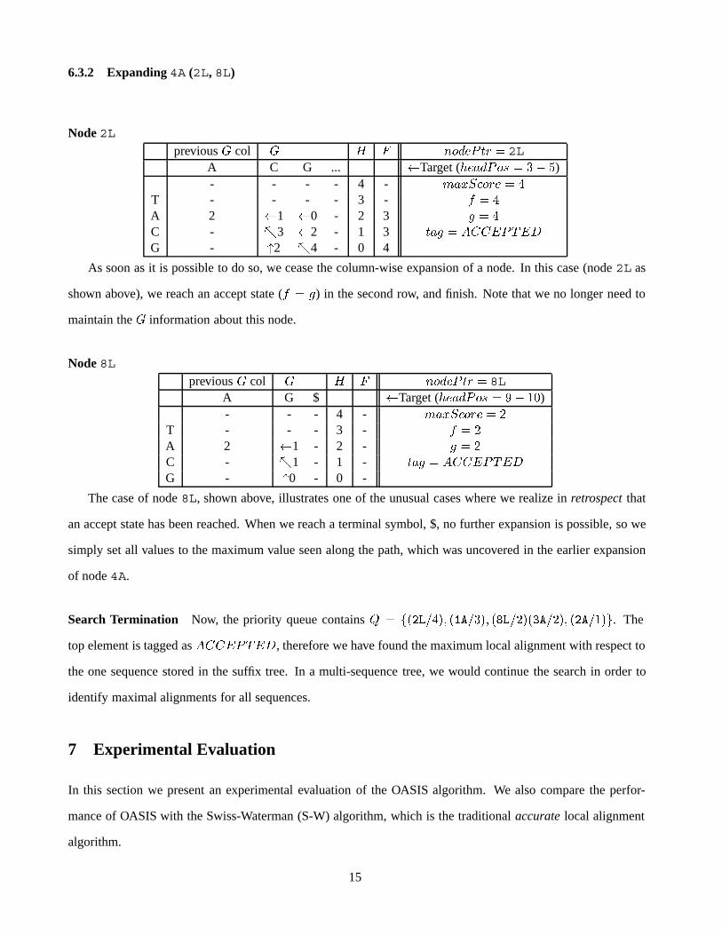
6.3.2 Expanding 4A (2L, 8L)

Node 2Lprevious � col � & ( ��)�* �� � 2L

A C G ... �Target ( ��)*�� � � �)- - - - 4 - ��" ���� � �

T - - - - 3 - $ � �

A 2 �1 �0 - 2 3 � � �

C - �3 �2 - 1 3 ��� � �//.*�.�G - 2 �4 - 0 4

As soon as it is possible to do so, we cease the column-wise expansion of a node. In this case (node 2L as

shown above), we reach an accept state ($ � �) in the second row, and finish. Note that we no longer need to

maintain the � information about this node.

Node 8Lprevious � col � & ( ��)�* �� � 8L

A G $ �Target ( ��)*�� � �� ��)- - - 4 - ��" ���� � �

T - - - 3 - $ � �

A 2 �1 - 2 - � � �

C - �1 - 1 - ��� � �//.*�.�G - 0 - 0 -

The case of node 8L, shown above, illustrates one of the unusual cases where we realize in retrospect that

an accept state has been reached. When we reach a terminal symbol, $, no further expansion is possible, so we

simply set all values to the maximum value seen along the path, which was uncovered in the earlier expansion

of node 4A.

Search Termination Now, the priority queue contains � � ����#��' ���# �' ���#�����#��' ���#���. The

top element is tagged as �//.*�.�, therefore we have found the maximum local alignment with respect to

the one sequence stored in the suffix tree. In a multi-sequence tree, we would continue the search in order to

identify maximal alignments for all sequences.

7 Experimental Evaluation

In this section we present an experimental evaluation of the OASIS algorithm. We also compare the perfor-

mance of OASIS with the Swiss-Waterman (S-W) algorithm, which is the traditional accurate local alignment

algorithm.

15

7.1 Experimental Setup and Implementation Details

All experiments were run on a Linux 2.4.13 machine with 896 MB of memory, a 1.70 GHz Intel Xeon processor,

and a Fujitsu MAN3367MP hard drive with a SCSI interface and a 40 GB capacity.

We implemented both OASIS and S-W in C++. Both code sets were compiled with full optimization using

gcc. For OASIS, we limited main memory usage to 256MB for these experiments, using a simple LRU buffer

pool system. The implementation used a block size of 2K to swap portions of the suffix tree index structure

between main memory and disk as necessary.

7.2 Data Set and Queries

For the data set in these experiments, we used the entire Swiss protein database [13]. Samples of four proteins

in this data set are shown in Figure 4. This data set is an annotated collection of proteins with low redundancy,

and is commonly used in practice. The database contains over 100K sequences, totaling roughly 40M protein

symbols, ranging in length from 7 to 2048 symbols. The proteins are represented as sequences, consisting of

symbols representing the 20 amino acids, or residues.

>gi|2495000|sp|Q63931|CCKR CAVPO CHOLECYSTOKININ TYPE A RECEPTOR (CCK-A RECEP-

TOR) (CCK-AR)

MDVVDSLFVNGSNITSACELGFENETLFCLDRPRPSKEWQPAVQILLYSLIFLLSVLGNTLVITVLIRNKRMRTVTNIFL

LSLAVSDLMLCLFCMPFNLIPSLLKDFIFGSAVCKTTTYFMGTSVSVSTFNLVAISLERYGAICKPLQSRVWQTKSHALK

VIAATWCLSFTIMTPYPIYSNLVPFTKNNNQTGNMCRFLLPNDVMQQTWHTFLLLILFLIPGIVMMVAYGLISLELYQGI

KFDAIQKKSAKERKTSTGSSGPMEDSDGCYLQKSRHPRKLELRQLSPSSSGSNRINRIRSSSSTANLMAKKRVIRMLIVI

VVLFFLCWMPIFSANAWRAYDTVSAERHLSGTPISFILLLSYTSSCVNPIIYCFMNKRFRLGFMATFPCCPNPGTPGVRG

EMGEEEEGRTTGASLSRYSYSHMSTSAPPP

>gi|1708198|sp|P80487|HHP THICU HETEROTROPH-SPECIFIC PROTEIN

AADDVTVVIGSAAPMSGPQ

>gi|13878750|sp|Q9CDN0|RS18 LACLA 30S ribosomal protein S18

MAQQRRGGFKRRKKVDFIAANKIEVVDYKDTELLKRFISERGKILPRRVTGTSAKNQRKVVNAIKRARVMALLPFVAEDQN

>gi|13878816|sp|Q9CI15|TIG LACLA Trigger factor (TF)

MTVSFEKTSDTKGTLSFSIDQETIKTGLDKAFNKVKANISVPGFRKGKISRQMFNKMYGEEALFEEALNAVLPTAYDAAV

KEAGIEPVAQPKIDVAKMEKGSDWELTAEVVVKPTVSLGDYKDLTVEVEATKEVSDEEVETRLTNSQNNLAELVVKETAA

ENGDTVVIDFVGSVDGVEFEGGKGSNHSLELGSGQFIPGFEEQLVGTKAGETVEVKVTFPENYQAEDLAGKEALFVTTVN

EVKAKELPELDDELAKDIDEEVETLDELKAKFRKELEESKAEAYNDAVETAAIEAAVANAEIKEIPEEMIHEEVHRAMNE

FLGGMQQQGISPEMYFQITGTSEDDLHKQYEADADKRVRTNLVIEAIAAAENFTTSDEEVKAEIEDLAGQYNMPVEQVEK

LLPVDMLKHDIAMKKAVEVIATTAKVK...

Figure 4: Portion of swissprot database

For our experiments, we used a query workload consisting of 500 queries. The queries were randomly

16

selected from the ProClass database of functional motifs [11]. The ProClass Database is a non-redundant

database which organizes the Swiss Protein data base according to family relationships (organizing similar

proteins in the same family class). So our queries represent the scenario where the scientist is querying a

protein database looking for short matches; such queries are frequently used to find matches to short peptide

sequences [8] 1. A simple definition of a peptide is two or more amino acids covalently linked by an amide bond

between two specific groups of the amino acids (the carboxylic and the alpha-amino groups). A simpler view of

the peptide is that it is a short sequence of amino acids.

The ProClass database contains roughly 70K motifs, ranging in length from 3 to 80 residues, with an

average length of 17.

In our experiments, we used three different edit matrices: a unit edit matrix (like Table 1 but for the 20 amino

acid symbols), and the BLOSUM90 and BLOSUM62 (for instance Figure 5) matrices; the BLOSUM matrices

are frequently used by life science researchers. We also varied the “selectivities” of the queries. The selectivities

are varied using the following technique: One of the inputs to the algorithm is �� ����, which determines

the minimum score of alignments to return. The selectivity is controlled using the minimum score ratio, which

indicates the ratio of the maximum possible alignment score we will accept. For instance, given the example

query “TACG” and unit edit distance, 4 is the maximum possible alignment score with any arbitrary sequence.

Given a ratio of 0.5, we would search for alignments with score � � ��� � � and above. Note that a ratio of 0

returns the entire database, which is typically not a very useful query.

A suffix tree was constructed on the entire Swiss protein data sets. The suffix tree was constructed in 17

passes, resulting in a 500MB structure. This construction phase took roughly 3.5 hours.

7.3 Experimental Goals

The experiments are intended to test and demonstrate the following issues:

� What are the tradeoffs between S-W and suffix-tree local alignment approaches?

� To what extent does the edit matrix influence performance? The intuition here is that a more homoge-

neous matrix, i.e. one that discriminates little between symbols, will result in less differentiation between

different paths, and thus a higher degree of branching in the search. We performed tests using a unit

1The approximate matches using BLAST has two versions for matching proteins, one for queries 5-15 residues longer, and the

other for 15 residues or longer sequences). Similarly there are two versions of BLAST for querying nucleotide (genetic) sequences

corresponding to short queries, which are 7-20 base pairs, and long queries, which are larger than 20 base pairs.

17

edit distance matrix (e.g Table 1), BLOSUM90, and BLOSUM62 (see Figures 5), which progressively

admit greater differences between target and query. BLOSUM matrices indicate the degree of similarity

between two distantly related protein sequences. The different degrees of BLOSUM matrices, e.g. 62%

in BLOSUM62, indicate that sequences with 62% similarity are given the greatest weight in generating

the matrix. As such, lower values favor more distantly related protein sequences[10]. These matrices are

commonly used by biologists as distance metrics for the BLAST and FASTA algorithms.

� To what extent does the length of the query influence performance? With S-W, the relationship between

query length and processing time is linear. With our algorithm, the influences are more complicated, as

the degree of “redundancy” is highest at lower tree depths. We explore this issue in more detail in the

following section.

7.3.1 The Effect of Redundancy on OASIS

OASIS exploits the redundancy found in most finite alphabet sequences. When an arc in the suffix tree is

expanded, each symbol along that arc can refer to multiple symbols in the database. Of course, a single symbol

in the database is also represented in multiple positions in the tree, since it will appear in multiple suffixes!

For instance, the ‘A’ at ��)*�� � in Figure 2 exists on 4 separate paths! We will present a simplified

mathematical model of the situation, to help explain the degradation of performance with longer queries, and

the expected improvement of the algorithm’s performance as the database size increases.

We will make two simplifying assumptions:

� Assume that the database is composed of random sequences of symbols, where symbols are selected uni-

formly from the alphabet �, independent of context. � is again the sum length of the database sequences.

� Assume that we are not allowing insertions and deletions, and the depth of the search is thus strictly

bounded by the length of the query. Note that by depth, we mean the length of the path, e.g. node 8L in

Figure 2 has depth 4.

Given a query length �, it is clear that in a full �-depth tree search, every symbol in the database can be

“visited” at most � times, since � suffixes will contain that symbol within a depth of �. Again, each symbol

in the tree can refer to multiple sequences or parts of sequences. How many exactly? It turns out the answer

depends on the depth in the tree. At depth one, the intuition is straightforward: given the uniformity assumption,

18

# Matrix made by matblas from blosum62.iij# * column uses minimum score# BLOSUM Clustered Scoring Matrix in 1/2 Bit Units# Blocks Database = /data/blocks_5.0/blocks.dat# Cluster Percentage: >= 62# Entropy = 0.6979, Expected = -0.5209

A R N D C Q E G H I L K M F P S T W Y V B Z X *A 4 -1 -2 -2 0 -1 -1 0 -2 -1 -1 -1 -1 -2 -1 1 0 -3 -2 0 -2 -1 0 -4R -1 5 0 -2 -3 1 0 -2 0 -3 -2 2 -1 -3 -2 -1 -1 -3 -2 -3 -1 0 -1 -4N -2 0 6 1 -3 0 0 0 1 -3 -3 0 -2 -3 -2 1 0 -4 -2 -3 3 0 -1 -4D -2 -2 1 6 -3 0 2 -1 -1 -3 -4 -1 -3 -3 -1 0 -1 -4 -3 -3 4 1 -1 -4C 0 -3 -3 -3 9 -3 -4 -3 -3 -1 -1 -3 -1 -2 -3 -1 -1 -2 -2 -1 -3 -3 -2 -4Q -1 1 0 0 -3 5 2 -2 0 -3 -2 1 0 -3 -1 0 -1 -2 -1 -2 0 3 -1 -4E -1 0 0 2 -4 2 5 -2 0 -3 -3 1 -2 -3 -1 0 -1 -3 -2 -2 1 4 -1 -4G 0 -2 0 -1 -3 -2 -2 6 -2 -4 -4 -2 -3 -3 -2 0 -2 -2 -3 -3 -1 -2 -1 -4H -2 0 1 -1 -3 0 0 -2 8 -3 -3 -1 -2 -1 -2 -1 -2 -2 2 -3 0 0 -1 -4I -1 -3 -3 -3 -1 -3 -3 -4 -3 4 2 -3 1 0 -3 -2 -1 -3 -1 3 -3 -3 -1 -4L -1 -2 -3 -4 -1 -2 -3 -4 -3 2 4 -2 2 0 -3 -2 -1 -2 -1 1 -4 -3 -1 -4K -1 2 0 -1 -3 1 1 -2 -1 -3 -2 5 -1 -3 -1 0 -1 -3 -2 -2 0 1 -1 -4M -1 -1 -2 -3 -1 0 -2 -3 -2 1 2 -1 5 0 -2 -1 -1 -1 -1 1 -3 -1 -1 -4F -2 -3 -3 -3 -2 -3 -3 -3 -1 0 0 -3 0 6 -4 -2 -2 1 3 -1 -3 -3 -1 -4P -1 -2 -2 -1 -3 -1 -1 -2 -2 -3 -3 -1 -2 -4 7 -1 -1 -4 -3 -2 -2 -1 -2 -4S 1 -1 1 0 -1 0 0 0 -1 -2 -2 0 -1 -2 -1 4 1 -3 -2 -2 0 0 0 -4T 0 -1 0 -1 -1 -1 -1 -2 -2 -1 -1 -1 -1 -2 -1 1 5 -2 -2 0 -1 -1 0 -4W -3 -3 -4 -4 -2 -2 -3 -2 -2 -3 -2 -3 -1 1 -4 -3 -2 11 2 -3 -4 -3 -2 -4Y -2 -2 -2 -3 -2 -1 -2 -3 2 -1 -1 -2 -1 3 -3 -2 -2 2 7 -1 -3 -2 -1 -4V 0 -3 -3 -3 -1 -2 -2 -3 -3 3 1 -2 1 -1 -2 -2 0 -3 -1 4 -3 -2 -1 -4B -2 -1 3 4 -3 0 1 -1 0 -3 -4 0 -3 -3 -2 0 -1 -4 -3 -3 4 1 -1 -4Z -1 0 0 1 -3 3 4 -2 0 -3 -3 1 -1 -3 -1 0 -1 -3 -2 -2 1 4 -1 -4X 0 -1 -1 -1 -2 -1 -1 -1 -1 -1 -1 -1 -1 -1 -2 0 0 -2 -1 -1 -1 -1 -1 -4* -4 -4 -4 -4 -4 -4 -4 -4 -4 -4 -4 -4 -4 -4 -4 -4 -4 -4 -4 -4 -4 -4 -4 1

Figure 5: BLOSUM62 Edit Matrix

precisely �

��� of suffixes begin with any given symbol. Extending the argument, we expect precisely �

����of

suffixes to begin with any arbitrary sequence of two symbols. The number of suffixes in the tree is equal to �,

so in general, we expect each symbol at depth ) in the tree to refer to �����

different positions in the database.

Making the assumption that each �-length query will require a full �-depth search through the suffix tree,

and the above relationships, we can expect to expand as much as������

�times as many columns as S-W using the

suffix tree approach! This is mitigated by two important factors: node pruning, and the fact that in practice, the

boundary of the search space (which this formula alludes to) is in practice very sparse. The critical observations

here however are that the worst-case suffix tree performance should improve with respect to S-W as the database

19

size increases, and degrade with the length of the query!

Pruning significantly improves algorithm performance of course. Although a mathematical analysis of this

issue is beyond the scope of this paper, we should note that deep nodes, while more dangerous, also have a greater

likelihood of being pruned, for the following reason: the $ -values become more accurate as we descend the tree,

since the optimistic heuristic portion has a lower and lower contribution. In essence, there is an increasing

chance of pruning paths that will eventually lead to low scores as we gain more information along those paths.

Experimental evaluation reveals a less drastic increase in running time as the query length increases (see Section

7.4).

On average, OASIS expands only 4.6% as many columns as S-W. In our experiments, in the worst-case

twice as many columns were expanded by OASIS, though this is counteracted somewhat by alignment pruning:

OASIS frequently does less work per column.

7.4 Experimental Results

In this section, we present the experimental results comparing OASIS with S-W. Since each data point in our

experiment represents a collection of 500 queries, we will present the results using “whisker” plots. Figure 6

describes the components of a whisker plot.

1.5 times inter-quartile r

1.5 times inter-quartile r

medianlower quartile

upper quartile

outliers

outliersS−W ratio=0.4 0.5 0.6 0.7 0.8 0.9

10−1

100

101

102

Tim

e to

fin

d al

l mat

ches

(se

c.)

Experiment description

Figure 6: Whisker Plot LegendFigure 7: Unit Edit Distance: Total Running Times(Log Scale)

Figures 7 to 9 show whisker plots of the time taken to run full queries for various selectivities, with time

shown on a logarithmic scale. For instance, for ratio = 0.7 all sequences with alignment scores greater than or

equal to 0.7 times the maximum possible alignment score are returned. As a point of reference, we also show

20

the running times for Smith-Waterman, which are not influenced by the selectivity, or the edit matrix for that

matter.

As can be observed from these figures, the OASIS algorithm is an order of magnitude faster than the

S-W algorithms in many cases, and even a few order of magnitude faster in some cases! As the selectivity

of the query increases (larger ratios) the relative performance of OASIS over S-W increases rapidly. The less

“relaxed” the edit matrix is in terms of admitting distantly related proteins (e.g. unit edit distance matrix and

BLOSUM90), the higher is the relative performance improvement from using OASIS.

S−W ratio=0.4 0.5 0.6 0.7 0.8 0.9

10−1

100

101

102

Tim

e to

fin

d al

l mat

ches

(se

c.)

Experiment descriptionS−W ratio=0.4 0.5 0.6 0.7 0.8 0.9

100

101

102

Tim

e to

fin

d al

l mat

ches

(se

c.)

Experiment description

Figure 8: BLOSUM90: Total Running Times (LogScale)

Figure 9: BLOSUM62: Total Running Times (LogScale)

At the same time, we also see in these figures that there are “expensive” outliers for OASIS, especially

for low selectivity queries, and more “relaxed” edit matrices (such as BLOSUM62). In many cases, these

expensive outliers generally corresponded to queries that were larger than 40 amino acids. Consequently, a

simple rule of thumb can be used is to switch to using the S-W algorithm for large query sequences (or use an

approximate matching algorithm such as BLAST). Note that as per the analysis in Section 7.3.1, this tradeoff

point is influenced by the size of the database, and as the size of the database increases, it is expected that this

tradeoff point will move to a larger number, making OASIS the preferred choice for larger queries.

In many other cases, the expensive outliers were associated with queries producing large numbers of matches.

We anticipate that in online searches, users will choose to terminate such low-discrimination queries after the

top results have been returned.

21

7.4.1 Effect of Query Length

Figure 10 illustrates the effect of query length on running times, for a minimum score ratio of 0.7. Each point

represents the mean running time for queries of each observed length. Notice that while S-W running times

increase linearly with respect to query length, OASIS exhibits super-linear behavior. This speaks to the inherent

tradeoffs involved in the use OASIS, or any search algorithm that makes use of a hierarchical structure to drive

the search process. Fortunately, in practice, performance does not appear to degrade in the worst-case fashion

according to the theoretical analysis.

10 15 20 25 30 35 400

50

100

150

200

250

300

Query length

Mea

n tim

e (s

ec.)

Unit edit matrixBLOSUM90BLOSUM62S−W

0 10 20 30 40 50 60 7010

−2

10−1

100

101

102

Number of results returned

Tim

e (s

ec.)

Unit edit matrixBLOSUM90BLOSUM62S−W

Figure 10: Mean Time by Query Length (Unit EditDistance Matrix)

Figure 11: Times for Online Results Generation(Log scale), Query: CLNTLGSYKCSC

7.4.2 Online Characteristics

The results presented in the previous sections describe the complete running times of the algorithm: the algo-

rithm continues running until it is certain that no branches can produce alignments scoring above the specified

minimum, but returns results online in descending score order. Top results are returned far more quickly. For

instance, the top scoring alignment was returned in under 0.5 seconds on average for all experiments reported

in the previous sections. The top 100 database targets were returned in under 7 seconds on average. In contrast,

algorithms such as S-W and the approximate BLAST searches, cannot provide this information until the full run

is completed.

In this section, we now examine the online behavior of OASIS. We illustrate the online behavior of OASIS

with a single query; however the behavior described here is also typical for other queries. We use the following

12 symbol long query for this experiment: CLNTLGSYKCSC. In this experiment, the “ratio” parameter in OASIS

22

was set to 0.7, which produced 8, 43 and 69 matches for the unit edit distance, BLOSUM90 and BLOSUM62

cases respectively. The results using this query are shown in Figure 11. Note that there are several plateaus

in the plot, resulting from accepted paths pointing to multiple sequences. As can be observed from this figure,

OASIS returns the top few results very quickly, making it well suited for use in an online setting.

8 Conclusion and Future Work

We have introduced a new algorithm called OASIS which improves upon the performance of the existing state

of the art for accurate local sequence alignment. The existing accurate local-alignment algorithm, the Smith-

Waterman (S-W) algorithm, is rarely used since it is considered to be too computationally expensive. Scientists

often settle for approximate search algorithms, which though finely tuned to avoid missing good matches, do

not guarantee that a good match will never be missed. In this paper we show that the OASIS algorithm is often

an order-of-magnitude (or more) faster than the S-W algorithm when the query is a short sequence. Such sort

sequences are frequently used in querying protein and genetic data sets, and we show that OASIS is extremely

effective in these cases.

Besides not missing any matches, OASIS, also has the property of returning result tuples in decreasing order

of the matching scores. Consequently, OASIS can also be uses in an online mode, where the scientist may want

to abort the query after seeing the top few results.

As part of future work, we plan on adapting the tree construction algorithm to allow for incremental updates.

This would allow updates to the database to incorporated into the index in a more efficient fashion that having to

rebuild the entire index. We also plan on investigating techniques to further improve the performance of OASIS

to answer longer queries. Finally we also plan on investigating techniques to effectively run OASIS on parallel

architectures, especially when evaluating long queries.

References

[1] S. Altschul, W. Gish, W. Miller, E. Myers, and D. Lipman. Basic local alignment search tool. Journal ofMolecular Biology, 1990.

[2] Stefan Berchtold, Daniel A. Keim, and Hans-Peter Kriegel. The X-tree: An index structure for high-dimensional data. In T. M. Vijayaraman, Alejandro P. Buchmann, C. Mohan, and Nandlal L. Sarda, editors,Proceedings of the 22nd International Conference on Very Large Databases, pages 28–39, San Francisco,U.S.A., 1996. Morgan Kaufmann Publishers.

23

[3] P. Bieganski, J. Riedi, J. V. Carlis, and E. F. Retzel. Generalized suffix trees for biological sequence data:Applications and implementation. In Proceedings of the Twenty-Seventh Annual Hawaii InternationalConference on System Sciences, pages 35–44, 1994.

[4] Stefan Burkhardt, Andreas Crauser, Paolo Ferragina, Hans-Peter Lenhof, Eric Rivals, and Martin Vingron.q -gram based database searching using a suffix array (QUASAR). In RECOMB, pages 77–83, 1999.

[5] B. Cooper and M. Shadmon. The index fabric. Technical report, RightOrder Inc.http://www.rightorder.com, 2001.

[6] B. F. Cooper, N. Sample, M. J. Franklin, G. R. Hjaltason, and M. Shadmon. A fast index for semistructureddata. In Proceedings of the 27th VLDB Conference, 2001.

[7] R. Durbin, S. Eddy, A. Krogh, and G. Mitchison. Biological Sequence Analysis. Cambridge UniversityPress, 1998.

[8] National Center for Biotechnology Information. BLAST Program Selection Guide.http://www.ncbi.nlm.nih.gov/BLAST/producttable.html, June 2002.

[9] Robert Giegerich and Stefan Kurtz. From ukkonen to mccreight and weiner: A unifying view of linear-timesuffix tree construction. Algorithmica, 19(3):331–353, 1997.

[10] S. Henikoff and J. Henikoff. Amino acid substitution matrices from protein blocks. In Proc. Natl. AcademyScience 89(10), pages 915–919, 1992.

[11] H. Huang, C. Xiao, and C. Wu. Proclass protein family database. Nucleic Acids Research, 2000.

[12] Ela Hunt, Malcolm P. Atkinson, and Robert W. Irving. A database index to large biological sequences. InThe VLDB Journal, pages 139–148, 2001.

[13] European Bioinformatics Institute. SWISS-PROT Database. http://www.ebi.ac.uk/swissprot/, 2002.

[14] Stefan Kurtz. Reducing the space requirement of suffix trees. Software - Practice and Experience,29(13):1149–1171, 1999.

[15] Stefan Kurtz. Foundations of sequence analysis. citeseer.nj.nec.com/kurtz01foundations.html, 2001.

[16] Edward M. McCreight. A space-economical suffix tree construction algorithm. Journal of the ACM,23(2):262–272, 1976.

[17] D.R Morrison. Patricia - practical algorithm to retrieve information d in alphanumeric. Journal of theACM, 15:514–534, 1968.

[18] Michael Schindler. Practical huffman coding. http://www.compressconsult.com/huffman/.

[19] T.F. Smith and M.S. Waterman. Identification of common molecular subsequences. Journal of MolecularBiology, 1981.

[20] E. Ukkonen. Constructing suffix trees on-line in linear time. In J. van Leeuwen, editor, Proceedings of the12th IFIP World Computer Congress, pages 484–492, Madrid, Spain, 1992. North-Holland.

24