Embed Size (px)
Citation preview
HAL Id: hal-00773609https://hal.inria.fr/hal-00773609
Submitted on 14 Jan 2013
HAL is a multi-disciplinary open accessarchive for the deposit and dissemination of sci-entific research documents, whether they are pub-lished or not. The documents may come fromteaching and research institutions in France orabroad, or from public or private research centers.
L’archive ouverte pluridisciplinaire HAL, estdestinée au dépôt et à la diffusion de documentsscientifiques de niveau recherche, publiés ou non,émanant des établissements d’enseignement et derecherche français ou étrangers, des laboratoirespublics ou privés.
OBJCUT: EFFICIENT SEGMENTATION USINGTOP-DOWN AND BOTTOM-UP CUES
M. Pawan Kumar, Philip Torr, Andrew Zisserman
To cite this version:M. Pawan Kumar, Philip Torr, Andrew Zisserman. OBJCUT: EFFICIENT SEGMENTATION US-ING TOP-DOWN AND BOTTOM-UP CUES. IEEE Transactions on Pattern Analysis and MachineIntelligence, Institute of Electrical and Electronics Engineers, 2010. hal-00773609
1
OBJCUT: Efficient Segmentation using
Top-Down and Bottom-Up Cues
M. Pawan Kumar P.H.S. Torr A. Zisserman
Dept. of Eng. Science Dept. of Computing Dept. of Eng. Science
University of Oxford Oxford Brookes University Universityof Oxford
[email protected] [email protected] [email protected]
DRAFT
2
AbstractWe present a probabilistic method for segmenting instancesof a particular object category within an
image. Our approach overcomes the deficiencies of previous segmentation techniques based on traditional
grid conditional random fields (CRF), namely that (i) they require the user to provide seed pixels for the
foreground and the background; and (ii) they provide a poor prior for specific shapes due to the small
neighborhood size of gridCRF. Specifically, we automatically obtain the pose of the object in a given
image instead of relying on manual interaction. Furthermore, we employ a probabilistic model which
includes shape potentials for the object to incorporate top-down information that is global across the
image, in addition to the grid clique potentials which provide the bottom-up information used in previous
approaches. The shape potentials are provided by the pose ofthe object obtained using an object category
model. We represent articulated object categories using a novel layered pictorial structures model. Non-
articulated object categories are modelled using a set of exemplars. These object category models have
the advantage that they can handle large intra-class shape,appearance and spatial variation. We develop
an efficient method, OBJCUT, to obtain segmentations using our probabilistic framework. Novel aspects
of this method include: (i) efficient algorithms for sampling the object category models of our choice;
and (ii) the observation that a sampling-based approximation of the expected log likelihood of the model
can be increased by a single graph cut. Results are presentedon several articulated (e.g. animals) and
non-articulated (e.g. fruits) object categories. We provide a favorable comparison of our method with
the state of the art in object category specific image segmentation, specifically the methods of Leibe &
Schiele and Schoenemann & Cremers.
Index TermsObject Category Specific Segmentation, Conditional RandomFields, Generalized EM, Graph Cuts
I. INTRODUCTION
Image segmentation has seen renewed interest in the field of Computer Vision, in part due
to the arrival of new efficient algorithms to perform the segmentation [5], and in part due to
the resurgence of interest in object category detection [11], [26]. Segmentation fell from favor
due to an excess of papers attempting to solve ill posed problems with no means of judging
the result. In contrast, interleaved object detection and segmentation [4], [26], [29], [37], [45]
is both well posed and of practical use. Well posed in that theresult of the segmentation can
be quantitatively judged, e.g. how many pixels have been correctly and incorrectly assigned to
the object. Of practical use because image editing tools canbe designed that provide apower
assistto cut out applications like ‘Magic Wand’, e.g. “I know this is a horse, please segment it
for me, without the pain of having to manually delineate the boundary.”
The conditional random field (CRF) framework [25] provides a useful model of images for
DRAFT
3
segmentation and their prominence has been increased by theavailability of efficient publically
available code for their solution. The approach of Boykov and Jolly [5], and more recently
its application in a number of systems includingGrabCut by Rother et al. [34], strikingly
demonstrates that with a minimum of user assistance objectscan be rapidly segmented (e.g. by
employing user-specified foreground and background seed pixels). However samples from the
distribution defined by the commonly used gridCRFs (e.g. with 4 or 8-neighborhood) very rarely
give rise to realistic shapes and on their own are ill suited to segmenting objects. For example,
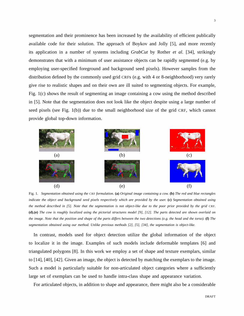
Fig. 1(c) shows the result of segmenting an image containinga cow using the method described
in [5]. Note that the segmentation does not look like the object despite using a large number of
seed pixels (see Fig. 1(b)) due to the small neighborhood size of the gridCRF, which cannot
provide global top-down information.
(a) (b) (c)
(d) (e) (f)
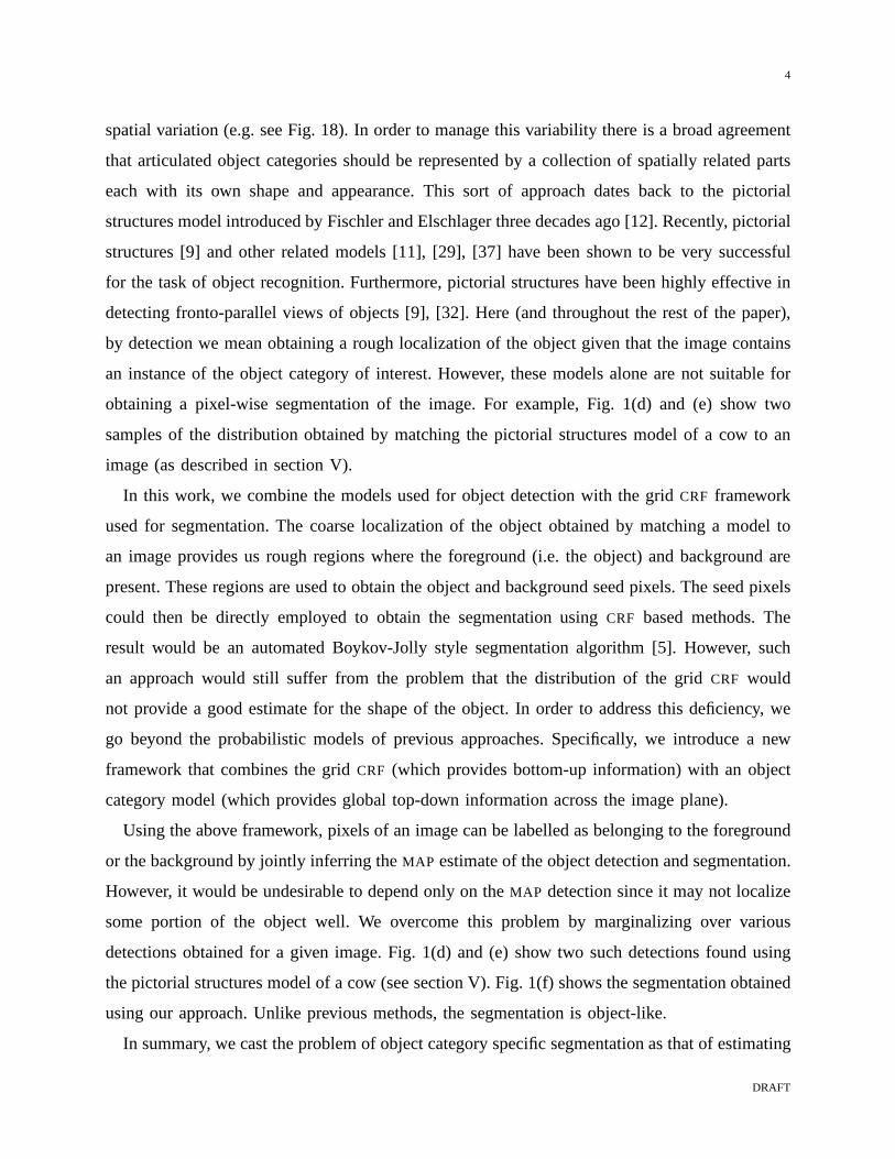
Fig. 1. Segmentation obtained using theCRF formulation.(a) Original image containing a cow.(b) The red and blue rectangles
indicate the object and background seed pixels respectively which are provided by the user.(c) Segmentation obtained using
the method described in [5]. Note that the segmentation is not object-like due to the poor prior provided by the gridCRF.
(d),(e) The cow is roughly localized using the pictorial structuresmodel [9], [12]. The parts detected are shown overlaid on
the image. Note that the position and shape of the parts differs between the two detections (e.g. the head and the torso).(f) The
segmentation obtained using our method. Unlike previous methods [2], [5], [34], the segmentation is object-like.
In contrast, models used for object detection utilize the global information of the object
to localize it in the image. Examples of such models include deformable templates [6] and
triangulated polygons [8]. In this work we employ a set of shape and texture exemplars, similar
to [14], [40], [42]. Given an image, the object is detected bymatching the exemplars to the image.
Such a model is particularly suitable for non-articulated object categories where a sufficiently
large set of exemplars can be used to handle intra-class shape and appearance variation.
For articulated objects, in addition to shape and appearance, there might also be a considerable
DRAFT
4
spatial variation (e.g. see Fig. 18). In order to manage thisvariability there is a broad agreement
that articulated object categories should be represented by a collection of spatially related parts
each with its own shape and appearance. This sort of approachdates back to the pictorial
structures model introduced by Fischler and Elschlager three decades ago [12]. Recently, pictorial
structures [9] and other related models [11], [29], [37] have been shown to be very successful
for the task of object recognition. Furthermore, pictorialstructures have been highly effective in
detecting fronto-parallel views of objects [9], [32]. Here(and throughout the rest of the paper),
by detection we mean obtaining a rough localization of the object given that the image contains
an instance of the object category of interest. However, these models alone are not suitable for
obtaining a pixel-wise segmentation of the image. For example, Fig. 1(d) and (e) show two
samples of the distribution obtained by matching the pictorial structures model of a cow to an
image (as described in section V).
In this work, we combine the models used for object detectionwith the grid CRF framework
used for segmentation. The coarse localization of the object obtained by matching a model to
an image provides us rough regions where the foreground (i.e. the object) and background are
present. These regions are used to obtain the object and background seed pixels. The seed pixels
could then be directly employed to obtain the segmentation using CRF based methods. The
result would be an automated Boykov-Jolly style segmentation algorithm [5]. However, such
an approach would still suffer from the problem that the distribution of the grid CRF would
not provide a good estimate for the shape of the object. In order to address this deficiency, we
go beyond the probabilistic models of previous approaches.Specifically, we introduce a new
framework that combines the gridCRF (which provides bottom-up information) with an object
category model (which provides global top-down information across the image plane).
Using the above framework, pixels of an image can be labelledas belonging to the foreground
or the background by jointly inferring theMAP estimate of the object detection and segmentation.
However, it would be undesirable to depend only on theMAP detection since it may not localize
some portion of the object well. We overcome this problem by marginalizing over various
detections obtained for a given image. Fig. 1(d) and (e) showtwo such detections found using
the pictorial structures model of a cow (see section V). Fig.1(f) shows the segmentation obtained
using our approach. Unlike previous methods, the segmentation is object-like.
In summary, we cast the problem of object category specific segmentation as that of estimating
DRAFT
5
a probabilistic model which consists of an object category model in addition to the gridCRF.
Put another way, the central idea of the paper is to incorporate a ‘shape prior’ (either non-
articulated or articulated) to the problem of object segmentation. We develop an efficient method,
OBJCUT, to obtain segmentations using this framework. The basis ofour method are two new
theoretical/algorithmic contributions: (i) we provide efficient algorithms for marginalizing or
optimizing the object category models of our choice; and (ii) we make the observation that
a sampling-based approximation of the expectation of the log likelihood of a CRF under the
distribution of some latent variables can be efficiently optimized by a single st-MINCUT.
Related Work: Many different approaches for segmentation using both top-down and bottom-
up information have been reported in the literature. We start by describing the methods which
require a limited amount of manual interaction. Huanget al. [19] describe an iterative algorithm
which alternates between fitting an active contour to an image and segmenting it on the basis
of the shape of the active contour. Cremerset al. [7] extend this by using multiple competing
shape priors and identifying the image regions where shape priors can be enforced. However,
the use of level sets in these methods makes them computationally inefficient. Freedmanet
al. [13] describe a more efficient algorithm based on st-MINCUT which uses a shape prior
for segmentation. However, note that in all the above methods the user provides the initial
shape of the segmentation. The quality of the solution heavily depends on a good initialization.
Furthermore, these methods are not suited for parts based models and cannot handle articulation.
There are a few automatic methods for combining top-down andbottom-up information.
For example, Borenstein and Ullman [4] describe an algorithm for segmenting instances of
a particular object category from images using a patch-based model learnt from training images.
Leibe and Schiele [26] provide a probabilistic formulationfor this while incorporating spatial
information of the relative locations of the patches. Winn and Jojic [44] describe a generative
model which provides the segmentation by applying a smooth deformation field on a class
specific mask. Shottonet al. [38] propose a novel texton-based feature which captures long
range interactions to provide pixel-wise segmentation. However, all the above methods use a
weak model for the shape of the object which does not provide realistic segmentations.
Winn and Shotton [45] present a segmentation technique using a parts-based model which
incorporates spatial information between neighboring parts. Their method allows for arbitrary
scaling but it is not clear whether their model is applicableto articulated object categories. Levin
DRAFT
6
and Weiss [27] describe an algorithm that learns a set of fragments for a particular object category
which assist the segmentation. The learnt fragments provide only local cues for segmentation
as opposed to the global information used in our work. The segmentation also relies on the
maximum likelihood estimate of the position of these fragments on a given test image (found
using normalized cross-correlation). This has two disadvantages:
• The spatial relationship between the fragments is not considered while matching them to an
image (e.g. it is possible that the fragment corresponding to the legs of a horse is located
above the fragment corresponding to the head). Thus the segmentation obtained would not
be object-like. In contrast, we marginalize over the objectcategory model while taking into
account the spatial relationships between the parts of the model.
• The algorithm becomes susceptible to error in the presence of background clutter. Indeed,
the segmentations provided by [27] assume that a rough localization of the object is known
a priori in the image. It is not clear whether normalized cross-correlation would provide
good estimates of the fragment positions in the absence of such knowledge.
More recently, Schoenemann and Cremers [35] proposed an approach to obtain the globally
optimal segmentation for a given shape prior. Although theyextended their framework to handle
large deformations [36], it still cannot handle articulated object categories such as humans and
quadrupeds. Moreover, it is not clear whether their approach can be extend to parts based models
which are known to provide an elegant representation of several object categories.
Outline: The paper is organized as follows. In section II the probabilistic model for object
category specific segmentation is described. Section III gives an overview of an efficient method
for solving this model for foreground-background labeling. We provide the details of our choice
of representations for articulated and non-articulated objects in section IV. The important issue of
automatically obtaining the samples of the object from a given image is addressed in section V.
Results for several articulated and non-articulated object categories and a comparison with other
methods is given in section VI.
A preliminary version of this paper has appeared as [23]. Since its publication, similar
techniques have been successfully applied for accurate object detection in [31], [33].II. OBJECT CATEGORY SPECIFIC SEGMENTATION MODEL
In this section we describe the model that forms the basis of our work. There are three issues
to be addressed in this section: (i) how to make the segmentation conform to foreground and
DRAFT
7
background appearance models; (ii) how to encourage the segmentation to follow edges within
the image; and (iii) how to encourage the outline of the segmentation to resemble the shape of
the object. We begin by briefly describing the model used in previous works [2], [5], [34].
Contrast Dependent Random Field:We denote the segmentation of an image by a labeling
function f(·) such that
f(a) =
0 if a is a foreground pixel,
1 if a is a background pixel.(1)
Given imageD, previous work on segmentation relies on a conditional random field (CRF) [25] or
equivalent contrast dependent random field (CDRF) [24] framework which models the conditional
distributionPr(f |D, θ). Hereθ denotes the parameters of theCDRF. By assuming the Markovian
property on the above distribution and using the Hammersley-Clifford theorem,Pr(f |D, θ) can
be written as
Pr(f |D, θ) =1
Z1(θ)exp(−Q1(f ;D, θ)), (2)
whereZ1(θ) is the partition function and the energyQ1(f ;D, θ) has the form
Q1(f ;D, θ) =∑
va∈v
θ1a;f(a) +
∑
(a,b)∈E
θpab;f(a)f(b) + θc
ab;f(a)f(b). (3)
The termsθ1a;f(a), θp
ab;f(a)f(b) and θcab;f(a)f(b) are called the unary, prior and contrast potentials
respectively. As in previous work [5], we define these terms as follows.
Unary Potential:The unary potentialθ1a;f(a) is the emission model for a pixel and is given by
θ1a;f(a) =
− log(Pr(Da|Hobj)) if f(a) = 0
− log(Pr(Da|Hbkg)) if f(a) = 1,(4)
whereHobj andHbkg are the appearance models for foreground and background respectively.
For this work,Hobj andHbkg are modelled asRGB distributions. The termDa denotes theRGB
values of the pixela.
Note that both the data independent prior termθpab;f(a)f(b) and the data dependent contrast term
θcab;f(a)f(b) are pairwise potentials (i.e. they are functions of two neighboring pixels). Below,
we provide the exact form of these terms separately while noting that their effect should be
understood together.
DRAFT
8
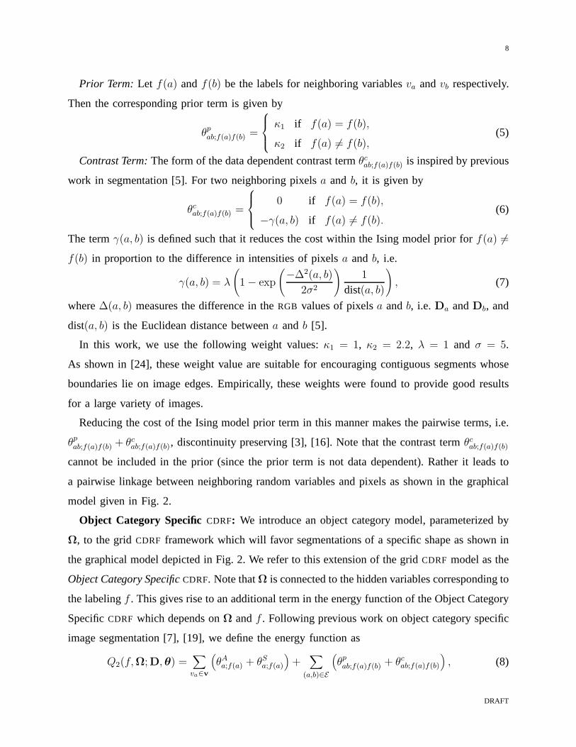
Prior Term: Let f(a) andf(b) be the labels for neighboring variablesva andvb respectively.
Then the corresponding prior term is given by
θpab;f(a)f(b) =
κ1 if f(a) = f(b),
κ2 if f(a) 6= f(b),(5)
Contrast Term:The form of the data dependent contrast termθcab;f(a)f(b) is inspired by previous
work in segmentation [5]. For two neighboring pixelsa and b, it is given by
θcab;f(a)f(b) =
0 if f(a) = f(b),
−γ(a, b) if f(a) 6= f(b).(6)
The termγ(a, b) is defined such that it reduces the cost within the Ising modelprior for f(a) 6=
f(b) in proportion to the difference in intensities of pixelsa andb, i.e.
γ(a, b) = λ
(
1− exp
(
−∆2(a, b)
2σ2
)
1
dist(a, b)
)
, (7)
where∆(a, b) measures the difference in theRGB values of pixelsa andb, i.e. Da andDb, and
dist(a, b) is the Euclidean distance betweena andb [5].
In this work, we use the following weight values:κ1 = 1, κ2 = 2.2, λ = 1 and σ = 5.
As shown in [24], these weight value are suitable for encouraging contiguous segments whose
boundaries lie on image edges. Empirically, these weights were found to provide good results
for a large variety of images.
Reducing the cost of the Ising model prior term in this mannermakes the pairwise terms, i.e.
θpab;f(a)f(b) + θc
ab;f(a)f(b), discontinuity preserving [3], [16]. Note that the contrast term θcab;f(a)f(b)
cannot be included in the prior (since the prior term is not data dependent). Rather it leads to
a pairwise linkage between neighboring random variables and pixels as shown in the graphical
model given in Fig. 2.
Object Category SpecificCDRF: We introduce an object category model, parameterized by
Ω, to the gridCDRF framework which will favor segmentations of a specific shapeas shown in
the graphical model depicted in Fig. 2. We refer to this extension of the gridCDRF model as the
Object Category SpecificCDRF. Note thatΩ is connected to the hidden variables corresponding to
the labelingf . This gives rise to an additional term in the energy functionof the Object Category
SpecificCDRF which depends onΩ andf . Following previous work on object category specific
image segmentation [7], [19], we define the energy function as
Q2(f,Ω;D, θ) =∑
va∈v
(
θAa;f(a) + θS
a;f(a)
)
+∑
(a,b)∈E
(
θpab;f(a)f(b) + θc
ab;f(a)f(b)
)
, (8)
DRAFT
9
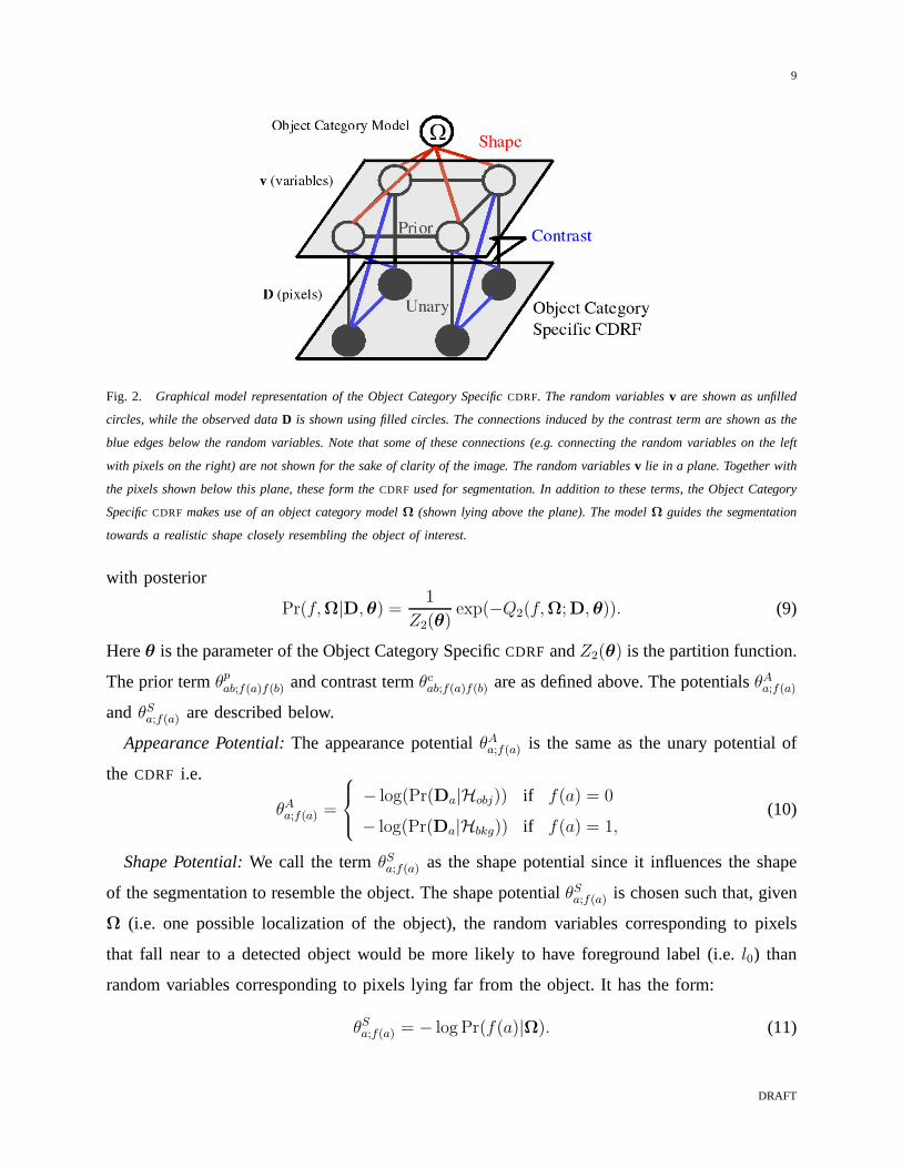
Fig. 2. Graphical model representation of the Object Category Specific CDRF. The random variablesv are shown as unfilled
circles, while the observed dataD is shown using filled circles. The connections induced by thecontrast term are shown as the
blue edges below the random variables. Note that some of these connections (e.g. connecting the random variables on the left
with pixels on the right) are not shown for the sake of clarityof the image. The random variablesv lie in a plane. Together with
the pixels shown below this plane, these form theCDRF used for segmentation. In addition to these terms, the Object Category
SpecificCDRF makes use of an object category modelΩ (shown lying above the plane). The modelΩ guides the segmentation
towards a realistic shape closely resembling the object of interest.
with posterior
Pr(f,Ω|D, θ) =1
Z2(θ)exp(−Q2(f,Ω;D, θ)). (9)
Hereθ is the parameter of the Object Category SpecificCDRF andZ2(θ) is the partition function.
The prior termθpab;f(a)f(b) and contrast termθc
ab;f(a)f(b) are as defined above. The potentialsθAa;f(a)
andθSa;f(a) are described below.
Appearance Potential:The appearance potentialθAa;f(a) is the same as the unary potential of
the CDRF i.e.
θAa;f(a) =
− log(Pr(Da|Hobj)) if f(a) = 0
− log(Pr(Da|Hbkg)) if f(a) = 1,(10)
Shape Potential:We call the termθSa;f(a) as the shape potential since it influences the shape
of the segmentation to resemble the object. The shape potential θSa;f(a) is chosen such that, given
Ω (i.e. one possible localization of the object), the random variables corresponding to pixels
that fall near to a detected object would be more likely to have foreground label (i.e.l0) than
random variables corresponding to pixels lying far from theobject. It has the form:
θSa;f(a) = − log Pr(f(a)|Ω). (11)
DRAFT
10
Following [7], [19], we choose to definePr(f(a)|Ω) as
Pr(f(a) = 0|Ω) ∝1
1 + exp(µ ∗ dist(a,Ω)), Pr(f(a) = 1|Ω) = 1− Pr(f(a) = 0|Ω), (12)
where dist(a,Ω) is the spatial distance of a pixela from the outline of the object defined byΩ
(being negative if inside the shape). The weightµ determines how much the pixels outside the
shape are penalized compared to the pixels inside the shape.
Hence, the modelΩ contributes the unary termθSa;f(a) for each pixela in the image for a
labeling f (see Fig. 2). Alternatively,Ω can also be associated with theCDRF using pairwise
terms as described in [13]. However, by reparameterizing the CDRF [18], both formulations can
be shown to be equivalent. We prefer the use of unary terms since they do not effect the submod-
ularity of the energy. Hence, it can easily be shown that the energy functionQ2(f,Ω;D, θ) can
be minimized via st-MINCUT [21]. Fig. 3 shows the advantage of introducing an object category
model in theCDRF.
(a) (b) (c)
(d) (e) (f)
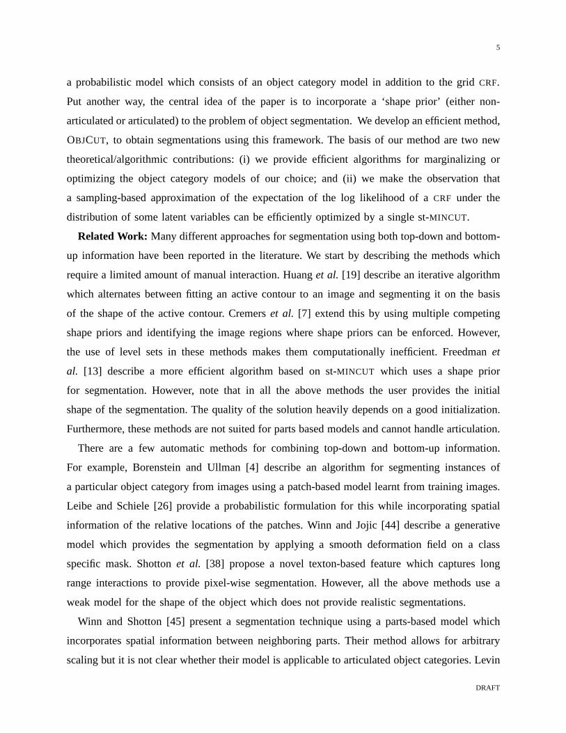
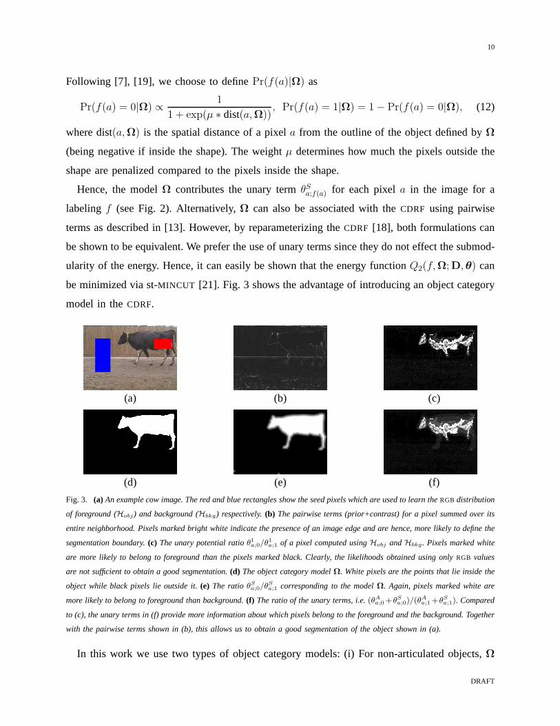
Fig. 3. (a) An example cow image. The red and blue rectangles show the seed pixels which are used to learn theRGB distribution
of foreground (Hobj) and background (Hbkg) respectively.(b) The pairwise terms (prior+contrast) for a pixel summed overits
entire neighborhood. Pixels marked bright white indicate the presence of an image edge and are hence, more likely to define the
segmentation boundary.(c) The unary potential ratioθ1a;0/θ1
a;1 of a pixel computed usingHobj andHbkg. Pixels marked white
are more likely to belong to foreground than the pixels marked black. Clearly, the likelihoods obtained using onlyRGB values
are not sufficient to obtain a good segmentation.(d) The object category modelΩ. White pixels are the points that lie inside the
object while black pixels lie outside it.(e) The ratioθSa;0/θS
a;1 corresponding to the modelΩ. Again, pixels marked white are
more likely to belong to foreground than background.(f) The ratio of the unary terms, i.e.(θAa;0 +θS
a;0)/(θAa;1 +θS
a;1). Compared
to (c), the unary terms in (f) provide more information aboutwhich pixels belong to the foreground and the background. Together
with the pairwise terms shown in (b), this allows us to obtaina good segmentation of the object shown in (a).
In this work we use two types of object category models: (i) For non-articulated objects,Ω
DRAFT

11
is represented by a set of exemplars; (ii) For articulated objects,Ω is specified by our extension
of the pictorial structures model [9], [12]. However, we note here that our methodology is
completely general and could be combined with any sort of object category model.
The Object Category SpecificCDRF framework defined above provides the probability of the
labeling f and the object category modelΩ as defined in equation (9). This is similar to the
model used by Huanget al. [19] and Cremerset al. [7]. However, our approach differs from
these works in the following respects: (i) in contrast to thelevel-sets based methods employed
in [7], [19], we develop an efficient algorithm based on st-MINCUT; (ii) we do not require an
accurate manual initialization to obtain the segmentation; and (iii) unlike [7], [19], we obtain
the foreground-background labeling by maximizing the posterior probabilityPr(f |D), instead
of the joint probabilityPr(f,Ω|D). In order to achieve this, we must integrate outΩ i.e.
Pr(f |D) =∫
Pr(f,Ω|D)dΩ. (13)
The surprising result of this work is that this intractable looking integral can in fact be optimized
by a simple and computationally efficient set of operations,as described in the next section.
III. ROADMAP OF THE SOLUTION
We now provide a high-level overview of our approach. Given an imageD, the problem
of segmentation requires us to obtain a labelingf ∗ which maximizes the posterior probability
Pr(f |D), i.e.
f ∗ = arg max Pr(f |D) = arg max log Pr(f |D). (14)
We have dropped the termθ from the above notation to make the text less cluttered. We note
however that there is no ambiguity aboutθ for the work described in this paper (i.e. it always
stands for the parameter of the Object Category SpecificCDRF). In order to obtain realistic
shapes, we would also like to influence the segmentation using an object category modelΩ (as
described in the previous section). Given an Object Category Specific CDRF specified by one
instance ofΩ, the required posterior probabilityPr(f |D) can be computed as
Pr(f |D) = Pr(f,Ω|D)Pr(Ω|f,D)
, (15)
⇒ log Pr(f |D) = log Pr(f,Ω|D)− log Pr(Ω|f,D), (16)
where Pr(f,Ω|D) is given by equation (9) andPr(Ω|f,D) is the conditional probability of
Ω given the image and its labeling. Note that we consider the log of the posterior probability
DRAFT
12
Pr(f |D). As will be seen, this allows us to marginalize the object category modelΩ using the
generalized Expectation Maximization (generalizedEM) [15] framework in order to obtaining
the desired labelingf ∗. By marginalizingΩ we would ensure that the segmentation is not
influenced by only one instance of the object category model (which may not localize the entire
object correctly, leading to undesirable effects such as inaccurate segmentation).
We now describe the generalizedEM framework which provides a natural way to deal with
Ω by treating it as missing (latent) data. The generalizedEM algorithm starts with an initial
estimatef 0 of the labeling and iteratively refines it by marginalizing over Ω. It has the desirable
property that during each iteration the posterior probability Pr(f |D) does not decrease (i.e.
the algorithm is guaranteed to converge to a local maximum).Given the current guess of the
labelingf ′, the generalizedEM algorithm consists of two steps: (i)E-step: where the probability
distributionPr(Ω|f ′,D) is obtained; and (ii)M-step: where a new labelingf is computed such
thatPr(f |D) ≥ Pr(f ′|D). We briefly describe how the two steps of the generalizedEM algorithm
can be computed efficiently in order to obtain the segmentation. We subsequently provide the
details for both the steps.
Efficiently Computing the E-step: Given the estimate of the labelingf ′, we approximate
the desired distributionPr(Ω|f ′,D) by sampling efficiently forΩ. For non-articulated objects,
this involves computing similarity measures at each location in the image. In§ V-A, we show
how this can be done efficiently. For the case of articulated objects, we develop an efficient
sum-product belief propagation algorithm in§ V-B, which efficiently computes the marginals
for a non regular Potts model (i.e. when the labels are not specified by an underlying grid of
parameters, complementing the result of Felzenszwalb and Huttenlocher [10]). As will be seen,
these marginals allow us to efficiently sample the object category model using a method similar
to [9].
Efficiently Computing the M-step: Once the samples ofΩ have been obtained in theE-step,
we need to compute a new labelingf such thatPr(f |D) ≥ Pr(f ′|D). We show that such a
labeling f can be computed by minimizing a weighted sum of energy functions of the form
given in equation (8), where the weighted sum over samples approximates the marginalization
of Ω (see below for details). The weights are given by the probability of the samples. This
allows the labelingf to be obtained efficiently using a single st-MINCUT operation [21].
Details: We concentrate on theM-step first. We will later show how theE-step can be
DRAFT
13
approximately computed using image features. Given the distribution Pr(Ω|f ′,D), we average
equation (16) overΩ to obtain
log Pr(f |D) = E(log Pr(f,Ω|D))−E(log Pr(Ω|f,D)), (17)
whereE(·) indicates the expectation underPr(Ω|f ′,D). The key observation of the generalized
EM algorithm is that the second term on the right side of equation (17), i.e.
E(log Pr(Ω|f,D)) =∫
(log Pr(Ω|f,D)) Pr(Ω|f ′,D)dΩ (18)
is maximized whenf = f ′ [15]. We obtain a labelingf such that it maximizes the first term
on the right side of equation (17), i.e.
f = arg maxE(log Pr(f,Ω|D)) = arg max∫
(log Pr(f,Ω|D)) Pr(Ω|f ′,D)dΩ. (19)
then, if f is different from f ′, it is guaranteed to increase the posterior probabilityp(f |D).
This is due to the following two reasons: (i)f increases the first term of equation (17), i.e.
E(log Pr(Ω, f |D)), as it is obtained by maximizing this term; and (ii)f decreases the second
term of equation (17), i.e.E(log Pr(Ω|f,D)), which is maximized whenf = f ′. If f is the
same asf ′ then the algorithm is said to have converged to a local maximum of the distribution
Pr(f |D). The expression in equation (19) is called the expected complete-data log-likelihood in
the generalizedEM literature.
In section V, it will be shown that we can efficiently sample from the object category modelΩ
of our choice. This suggests a sampling based solution to maximizing equation (19). Let the set
of s samples beΩ1, . . . ,Ωs, with weightswi = Pr(Ωi|f′,D). Using these samples equation (19)
can be approximated as
f = arg maxf
i=s∑
i=1
wi log Pr(f,Ωi|D,
= arg maxf
∑i=si=1 wi(−Q3(f,Ωi;D))− C, (20)
⇒ f = arg minf
∑i=si=1 wiQ3(f,Ωi;D) + C. (21)
The form of the energyQ3(f,Ωi;D) is given in equation (8). The termC =∑
i wi log Z3(θ)
is a constant which does not depend onf or Ω and can be therefore be ignored during the
minimization.This is the key equation of our approach.We observe that this energy function
is a weighted linear sum of the energiesQ3(f,Ω;D) which, being a linear combination with
DRAFT
14
positive weightswi, can also be optimized using a single st-MINCUT operation [21] (see Fig. 4).
This demonstrates the interesting result that forCDRF (and MRF) with latent variables, it is
computationally feasible to optimize the complete-data log-likelihood.
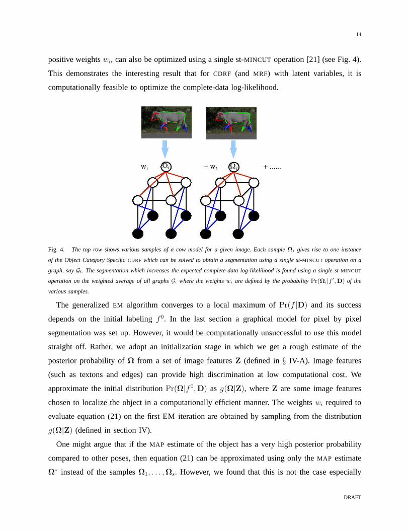
Fig. 4. The top row shows various samples of a cow model for a given image. Each sampleΩi gives rise to one instance
of the Object Category SpecificCDRF which can be solved to obtain a segmentation using a single st-MINCUT operation on a
graph, sayGi. The segmentation which increases the expected complete-data log-likelihood is found using a single st-MINCUT
operation on the weighted average of all graphsGi where the weightswi are defined by the probabilityPr(Ωi|f′, D) of the
various samples.
The generalizedEM algorithm converges to a local maximum ofPr(f |D) and its success
depends on the initial labelingf 0. In the last section a graphical model for pixel by pixel
segmentation was set up. However, it would be computationally unsuccessful to use this model
straight off. Rather, we adopt an initialization stage in which we get a rough estimate of the
posterior probability ofΩ from a set of image featuresZ (defined in§ IV-A). Image features
(such as textons and edges) can provide high discriminationat low computational cost. We
approximate the initial distributionPr(Ω|f 0,D) as g(Ω|Z), whereZ are some image features
chosen to localize the object in a computationally efficientmanner. The weightswi required to
evaluate equation (21) on the first EM iteration are obtainedby sampling from the distribution
g(Ω|Z) (defined in section IV).
One might argue that if theMAP estimate of the object has a very high posterior probability
compared to other poses, then equation (21) can be approximated using only theMAP estimate
Ω∗ instead of the samplesΩ1, . . . ,Ωs. However, we found that this is not the case especially
DRAFT

15
when theRGB distribution of the background is similar to that of the object. For example,
Fig. 15 shows various samples obtained by matching the modelfor a cow to two images. Note
that different samples localize different parts of the object correctly and have similar posterior
probabilities. Thus it is necessary to use multiple samplesof the object category model.
The roadmap described above results in the OBJCUT algorithm, which obtains object category
specific segmentation. Algorithms 1 and 2 summarize the mainsteps of OBJCUT for non-
articulated and articulated object categories respectively. Note that we can keep on iterating over
the E and theM steps. However, we observed that the samples (and the segmentation) obtained
from one iteration to the next do not differ substantially (e.g. see Fig. 16). Hence, we run each
step once for computational efficiency, as described in Algorithms 1 and 2. As will be seen in the
experiments, we obtain accurate results for different object categories using only one iteration
of the generalizedEM algorithm.
In the remainder of the chapter, we provide details of the object category modelΩ of our
choice. We propose efficient methods to obtain the samples from the posterior probability
distribution ofΩ required for the marginalization in equation (21). We demonstrate the results
on a number of articulated and non-articulated object categories.
IV. OBJECT CATEGORY MODELS
When choosing the modelΩ for the Object Category SpecificCDRF, two issues need to be
considered: (i) whether the model can handle intra-class shape and appearance variation (and, in
the case of articulated objects, spatial variation); and (ii) whether samples from the distribution
g(Ω|Z) (which are required for segmentation) can be obtained efficiently.
We represent theshapeof an object (or a part, in the case of articulated objects) using
multiple exemplars of the boundary. This allows us to handlethe intra-class shape variation.
The appearanceof an object (or part) is represented using multiple textureexemplars. Again,
this handles the intra-class appearance variation. Note that the exemplars model the shape and
appearance of an object category. These should not be confused with the shape and appearance
potentials of the Object Category SpecificCDRF used to obtain the segmentation.
Once an initial estimate of the object is obtained, its appearance is known. Thus the localization
of the object can be refined using a better appearance model (i.e. one which is specific to that
instance of the object category). For this purpose, we use histograms which define the distribution
of the RGB values of the foreground and the background.
DRAFT

16
• Input: An imageD and a non-articulated object category model.
• Initial estimate of pose using edges and texture (§ V-A.1):
1) A set of candidate posesto = (xo, yo, θo, σo) for the object is identified using a tree cascade of classifiers
which computes a set of image featuresZ.
2) The maximum likelihood estimate is chosen as initial estimate of the pose.
• Improved estimation of pose taking into account color (§ V-A.2):
1) The appearance model of both foreground and background isupdated.
2) A new set of candidate poses is generated for the object by densely sampling pose space around the estimate
found in the above step (again, using a tree cascade of classifiers for computingZ).
• The samplesΩ1, . . . ,Ωs are obtained from the posteriorg(Ω|Z) of the object category model as described in
§ V-A.3.
• OBJCUT
1) The weightswi = g(Ωi|Z) are computed.
2) The energy in equation (21) is minimized using a single st-MINCUT operation to obtain the segmentationf .
Algorithm 1: The OBJCUT algorithm for non-articulated object categories.
• Input: An imageD and an articulated object category model.
• Initial estimate of pose using edges and texture (§ V-B.1):
1) A set of candidate posesti = (xi, yi, θi, σi) for each part is identified using a tree cascade of classifiers
which computes a set of image featuresZ.
2) An initial estimate of the poses of the parts is found without considering the layering of parts using an
efficient sum-productBP algorithm (described in the Appendix).
• Improved estimation of pose taking into account color and occlusion (§ V-B.2):
1) The appearance model of both foreground and background isupdated.
2) A new set of candidate poses is generated for each part by densely sampling pose space around the estimate
found in the above step (again, using a tree cascade of classifiers for computingZ).
3) The pose of the object is estimated using efficient sum-product BP and the layering of the parts.
• The samplesΩ1, . . . ,Ωs are obtained from the posteriorg(Ω|Z) of the object category model as described in
§ V-B.3.
• OBJCUT
1) The weightswi = g(Ωi|Z) are computed.
2) The energy in equation (21) is minimized using a single st-MINCUT operation to obtain the segmentationf .
Algorithm 2: The OBJCUT algorithm for articulated object categories.
We define the modelΩ for non-articulated objects as a set of shape and texture exemplars (see
Fig. 5). In the case of articulated objects, one must also allow for considerable spatial variation.
For this purpose, we use the pictorial structures (PS) model. However, thePS models used in
previous work [9], [12] assume non-overlapping parts connected in a tree structure. We extend
the PS by incorporating the layering information of parts and connecting them in a complete
DRAFT

17
graph structure. We call the resulting representation thelayered pictorial structures(LPS) model.
Below, we describe the object category models in detail.
A. Set of Exemplars Model
We represent non-articulated object categories as 2D patterns with a probabilistic model for
their shape and appearance. The shape of the object categoryis represented using a set of shape
exemplarsS = S1,S2, · · · ,Se. For this work, each shape exemplarSi is given by a set of points
si;1, si;2, · · · , si;m describing the outline of the object. Similarly, the appearance is represented
using a set of texture exemplarsT = T1,T2, · · · ,Te, where each exemplar is an image patch
(i.e. a set of intensity values). Note that we use multiple exemplars (i.e.e > 1) to handle the
shape and appearance variations which are common in non-articulated object categories. We call
this the set of exemplars (SOE) model. Note that similar models were used for object detection
in [14], [40], [42].
1) Feature likelihood for object:Given the putative pose of an object, i.e.to = xo, yo, φo, ρo
(wherexo, yo is the location,φo is the rotation andρo is the scale), we computed two features
Z = z1, z2 for the shape and appearance of the object respectively. LetDo ⊆ D be the set
of pixels corresponding to the object at poseto. The featuresz1 and z2 are computed using
Do. Assuming independence of the two features, the likelihoodbased on the whole data is
approximated as
Pr(Z|Ω) = Pr(z1) Pr(z2) (22)
where Pr(z1) ∝ exp(−z1) and Pr(z2) ∝ exp(−z2). We also assume the priorPr(Ω) to be
uniform. This provides us with the distributiong(Ω|Z) as
g(Ω|Z) ∝ Pr(Z|Ω) Pr(Ω) ∝ Pr(Z|Ω). (23)
We now describe the featuresz1 andz2 in detail.
Outline (z1): The likelihood of the object shape should be robust to outliers resulting from
cluttered backgrounds. To this end, we definez1 as the minimum of the truncated chamfer
distances over all the exemplars of the object at poseto. Let U = u1, u2, · · · , um represent
the edges of the image atto. Thenz1 is computed asz1 = minSi∈S dcham(Si,U). The truncated
chamfer distancedcham(·, ·) is given bydcham(Si,U) = 1m
∑
j minmink ||uk − si;j||, τ1, where
τ1 is a threshold for truncation which reduces the effect of outliers and missing edges. Orientation
DRAFT

18
information is included by computingmink ||uk − si;j|| only over those edge pointsuk which
have a similar orientation tosi;j. This makes the chamfer distance more robust [14]. We use 8
orientation groups for the outline points.
Texture (z2): We use theVZ classifier [43] which provides a histogram representationHi for
each exemplarTi1. It also provides a histogramHo for the image patchDo. The featurez2 is
computed asz2 = minTi∈T dchi(Hi,Ho), wheredchi(·, ·) is theχ2 distance2.
2) Learning the exemplars:In order to learn the exemplars, we use manually segmented
images. The outline of each segmented image provides us withan exemplarsSi ∈ S. The
texture exemplarsTi are given by the subimage marked as foreground. We use 20 segmented
images each for the ‘banana’ and the ‘orange’ categories. A subset of the shape exemplarsS of
these two categories is shown in Fig. 5.
Fig. 5. A selection of the multiple exemplars used to represent the model for bananas and oranges. Multiple shape exemplars
are required to handle intra-class shape variability.
We now describe an extension to thePS which is used as the modelΩ for articulated objects.
B. Layered Pictorial Structures
In the case of articulated objects, we use thePS model to handle large deformations.PS are
compositions of 2D patterns, termedparts, under a probabilistic model for their shape, appearance
and spatial layout. However, thePS models used previously in [9], [12] are not directly suitable
for applications such as efficient segmentation due to the following reasons: (i) they use a weak
likelihood model which results in a large number of putativeposes for each part; (ii) the parts
are connected in a tree structure and hence, provide a weak spatial model; and (iii) they do not
explicitly model self-occlusion. Hence, different parts with similar shape and appearance (e.g.
1The VZ classifier obtains a texton dictionary by clustering intensity values in anN × N neighborhood of each pixel inTi
for all Ti ∈ T . The histogramHi is given by the frequency of each entry of this texton dictionary in Ti. We useN = 3 and
60 clusters in our experiments.
2The featurez2 described here handles the intra-class variation in appearance and is used to determine an initial estimate of
the pose of the object. This estimate is then refined using a better appearance model (i.e. specific to a particular instance of the
object category) as described in§ V-A.2.
DRAFT
19
the legs of cows or horses) are often incorrectly detected atthe same pose (i.e. even in cases
where they are actually at different poses in the given image).
We overcome the deficiencies of previousPS models by extending them in three ways: (i)
similar to SOE, the likelihood of a part includes both its outline and its texture which results
in a small number of putative poses for each part in a given image (see§ V-B.1); (ii) all parts
are connected to each other to form a complete graph instead of a tree structure which provides
a better spatial model; and (iii) similar to the model described in [1], each partpi is assigned
an occlusion numberoi which determines its relative depth. The occlusion numbersallow us to
explicitly model self-occlusion. Specifically, a partpi can partially or completely occlude part
pj if and only if oi > oj. Note that several parts can have the same occlusion number if they
are at the same depth. Such parts, which share a common occlusion number, are said to lie in
the same layer. We call this model layered pictorial structures (LPS).
1) Posterior of theLPS: An LPS can also be viewed as anMRF where the random variables of
the MRF correspond to thenP parts. Each random variable takes one ofnL labels which encode
the putative poses of the part. Similar to the pose of an object described in§ IV-A, the pose of
the ith part is defined by a labelti = xi, yi, φi, ρi. For a given poseti and imageD, the part
pi corresponds to the subset of the image pixelsD which are used to calculate featuresZi.
The posterior of theLPS is given by
g(Ω|Z) = Pr(Z|Ω) Pr(Ω), (24)
whereZ = Z1, . . . ,ZnP are the image features,p(Z|Ω) is the feature likelihood andp(Ω) is
the prior. Like theSOE model, the shape of anLPS is specified by a set of shape exemplarsSi
for each partpi. The appearance of anLPS is modelled using a set of texture exemplarsT for the
object category. Note that unlike the shape exemplars, which are specific to a part of an object
category, the texture exemplars are specific to the object category of interest. Assuming that the
featuresZi are computed by not including pixels accounted for by partspj for which oj > oi
(i.e. parts which can occludepi), the feature likelihood is given byPr(Z|Ω) =∏i=nP
i=1 Pr(Zi|Ω).
The feature likelihoodPr(Zi|Ω) for part pi is computed as described in§ IV-A.1. Specifically,
the likelihood of the first feature, i.e.Pr(z1), is computed using the minimum of the truncated
chamfer distance, over the setSi for the part, at poseti. The texture likelihood,p(z2), is obtained
DRAFT
20
from the VZ classifier using the setT for the object category3.
LPS, like PS, are characterized by pairwise only dependencies between the random variables.
These are modelled as a prior on the relative poses of parts:
Pr(Ω) ∝ exp
−i=nP∑
i=1
j=nP∑
j=1,j 6=i
α(ti, tj)
. (25)
Note that we use a completely connectedMRF as this was found to provide a better localization
of the object than a tree structuredMRF [22]. In our approach, the pairwise potentialsα(ti, tj)
of putative poses for each pair of parts are given by a non-regular Potts model, i.e.
α(ti, tj) =
d1 if valid configuration
d2 otherwise,(26)
where d1 < d2. In other words, all valid configurations are considered equally likely and
have a smaller cost. A configuration is considered valid if the difference between the two
posesti and tj lies in an interval defined bytminij = xmin
ij , yminij , θmin
ij , σminij and t
maxij =
xmaxij , ymax
ij , θmaxij , σmax
ij , i.e. tminij ≤ |ti − tj| ≤ t
maxij . Note that the above inequalities should
be interpreted component-wise (i.e.xminij ≤ |xi − xj | ≤ xmax
ij and so on). For each pair of parts
pi and pj the termstminij and t
maxij are learnt using training video sequences as described in
§ IV-B.2. Using equation (24), the posterior of theLPS parameters is given by
g(Ω|Z) ∝i=nP∏
i=1
Pr(Zi|Ω) exp
−∑
j 6=i
α(ti, tj)
. (27)
2) Learning theLPS: We now describe how we learn the various parameters of theLPS model
for cows. To this end, we use 20 cow videos of 45 frames each andlearn the shape, appearance
and transformations of rigidly moving segments in each frame of the video using the motion
segmentation method described in [24]. Correspondence between the segments learnt from two
different videos is established using shape context with continuity constraints [40] as shown
in Fig. 6. The corresponding segments then define a part of theLPS model. The outline of the
segments defines the shape exemplarsSi (see Fig. 7), while the intensity values of the segmented
cows provides the setT . Furthermore, an estimate of|ti − tj| is also obtained (after rescaling
3Again, the featurez2 described here handles the intra-class variation in appearance and is used to determine an initial estimate
of the pose of the object. This estimate is then refined using abetter appearance model (i.e. specific to a particular instance of
the object category) as described in§ V-B.2.
DRAFT
21
the frames of the video such that the width of the cows is230 pixels), for each frame and for
all pairs of partspi and pj. This is used to compute the parameterstminij and t
maxij that define
valid configurations.
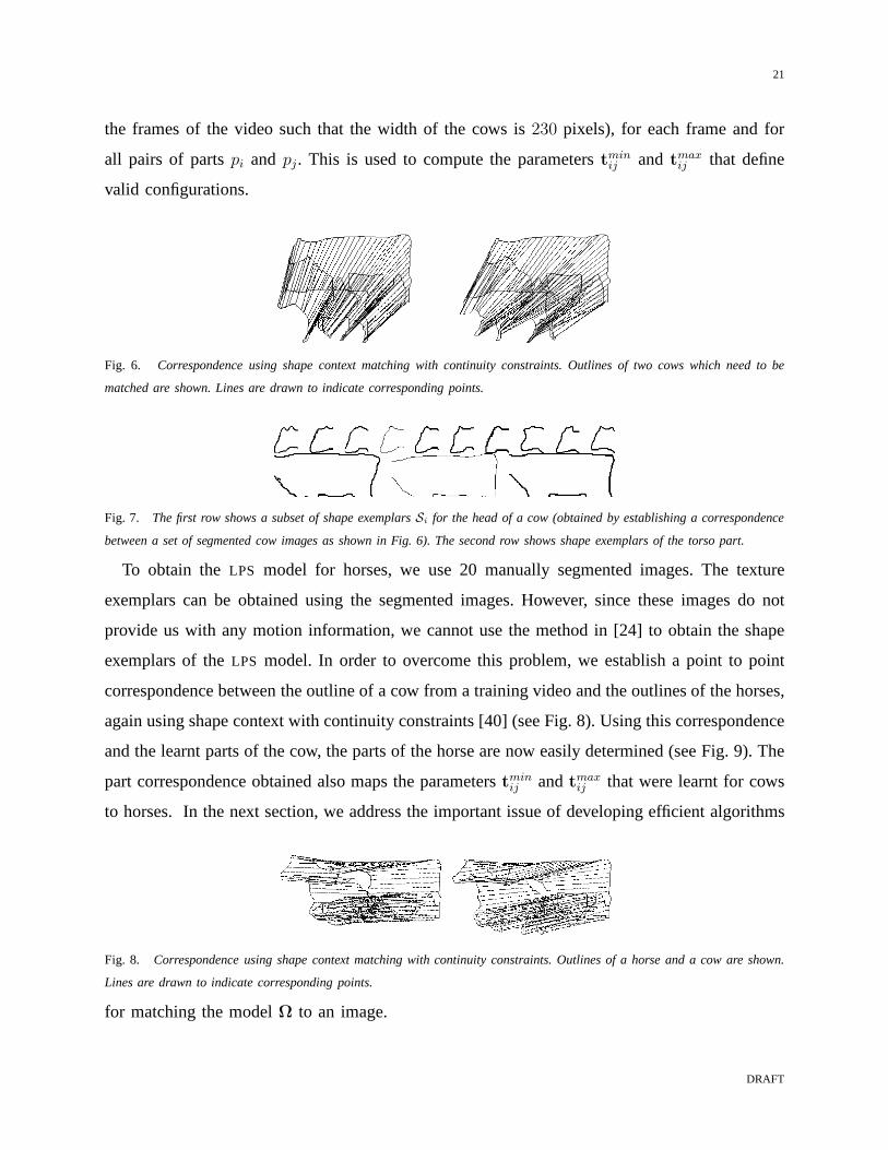
Fig. 6. Correspondence using shape context matching with continuity constraints. Outlines of two cows which need to be
matched are shown. Lines are drawn to indicate corresponding points.
Fig. 7. The first row shows a subset of shape exemplarsSi for the head of a cow (obtained by establishing a correspondence
between a set of segmented cow images as shown in Fig. 6). The second row shows shape exemplars of the torso part.
To obtain theLPS model for horses, we use 20 manually segmented images. The texture
exemplars can be obtained using the segmented images. However, since these images do not
provide us with any motion information, we cannot use the method in [24] to obtain the shape
exemplars of theLPS model. In order to overcome this problem, we establish a point to point
correspondence between the outline of a cow from a training video and the outlines of the horses,
again using shape context with continuity constraints [40](see Fig. 8). Using this correspondence
and the learnt parts of the cow, the parts of the horse are now easily determined (see Fig. 9). The
part correspondence obtained also maps the parameterstminij andt
maxij that were learnt for cows
to horses. In the next section, we address the important issue of developing efficient algorithms
Fig. 8. Correspondence using shape context matching with continuity constraints. Outlines of a horse and a cow are shown.
Lines are drawn to indicate corresponding points.
for matching the modelΩ to an image.
DRAFT

22
Fig. 9. The first and second row show the multiple exemplars of the head and the torso part respectively. The exemplars are
obtained by establishing a correspondence between segmented images of cows and horses as shown in Fig. 8.
V. SAMPLING THE OBJECT CATEGORY MODELS
Given an imageD, our objective is to match the object category model to it in order to obtain
samples from the distributiong(Ω|Z). We achieve this in three stages:
• Initialization, where we fit the object category model to a given imageD by computing
featuresz1 (i.e. chamfer) andz2 (i.e. texture) using exemplars. This provides us with a
rough object pose.
• Refinement, where the initial estimate is refined by computingz2 using a better appearance
model (i.e. theRGB distribution for the foreground and background learnt using the initial
pose together with the shape) instead of the texture featureused during initialization. In the
case of articulated objects, the layering information is also used.
• Sampling, where samples are obtained from the distributiong(Ω|Z).
A. Sampling theSOE
We now describe the three stages for obtaining samples by matching theSOE model (for a
non-articulated object category) to a given image.
1) Initial estimation of pose:In order to obtain the initial estimate of the pose of an object,
we need to compute the feature likelihood for each pose usingall exemplars. This would be
computationally expensive due to the large number of possible poses and exemplars. However,
most poses have a very low likelihood since they do not cover the pixels containing the object
of interest. We require an efficient method which discards such poses quickly. To this end, we
use atree cascade of classifiers[39].
We term the rotated and scaled versions of the shape exemplars astemplates. When matching
many similar templates to an image, a significant speed-up isachieved by forming a template
hierarchy and using a coarse-to-fine search. The idea is to group similar templates together
with an estimate of the variance of the error within the cluster, which is then used to define a
matching threshold. For each cluster, a prototype of the cluster is first compared to the image; the
DRAFT
23
individual templates within the cluster are compared to theimage only if the error is below the
threshold. This clustering is done at various levels, resulting in a hierarchy, with the templates
at the leaf level covering the space of all possible templates (see Fig. 10).
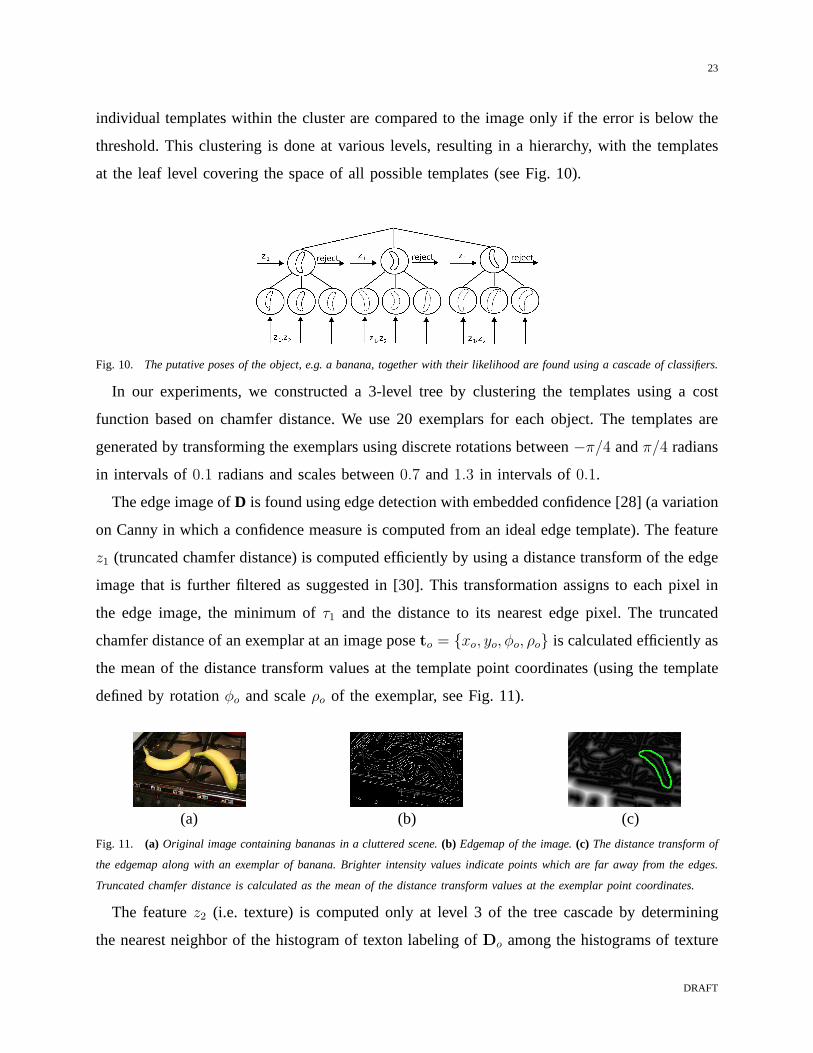
Fig. 10. The putative poses of the object, e.g. a banana, together with their likelihood are found using a cascade of classifiers.
In our experiments, we constructed a 3-level tree by clustering the templates using a cost
function based on chamfer distance. We use 20 exemplars for each object. The templates are
generated by transforming the exemplars using discrete rotations between−π/4 andπ/4 radians
in intervals of0.1 radians and scales between0.7 and1.3 in intervals of0.1.
The edge image ofD is found using edge detection with embedded confidence [28] (a variation
on Canny in which a confidence measure is computed from an ideal edge template). The feature
z1 (truncated chamfer distance) is computed efficiently by using a distance transform of the edge
image that is further filtered as suggested in [30]. This transformation assigns to each pixel in
the edge image, the minimum ofτ1 and the distance to its nearest edge pixel. The truncated
chamfer distance of an exemplar at an image poseto = xo, yo, φo, ρo is calculated efficiently as
the mean of the distance transform values at the template point coordinates (using the template
defined by rotationφo and scaleρo of the exemplar, see Fig. 11).
(a) (b) (c)
Fig. 11. (a) Original image containing bananas in a cluttered scene.(b) Edgemap of the image.(c) The distance transform of
the edgemap along with an exemplar of banana. Brighter intensity values indicate points which are far away from the edges.
Truncated chamfer distance is calculated as the mean of the distance transform values at the exemplar point coordinates.
The featurez2 (i.e. texture) is computed only at level 3 of the tree cascadeby determining
the nearest neighbor of the histogram of texton labeling ofDo among the histograms of texture
DRAFT
24
exemplars. For this purpose, we use the efficient nearest neighbor method described in [17]
(modified forχ2 distance instead of Euclidean distance).
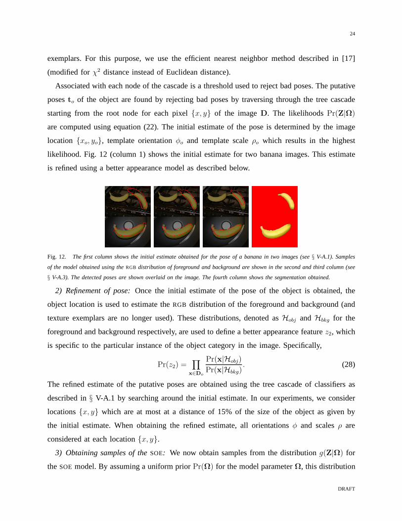
Associated with each node of the cascade is a threshold used to reject bad poses. The putative
posesto of the object are found by rejecting bad poses by traversing through the tree cascade
starting from the root node for each pixelx, y of the imageD. The likelihoodsPr(Z|Ω)
are computed using equation (22). The initial estimate of the pose is determined by the image
location xo, yo, template orientationφo and template scaleρo which results in the highest
likelihood. Fig. 12 (column 1) shows the initial estimate for two banana images. This estimate
is refined using a better appearance model as described below.
Fig. 12. The first column shows the initial estimate obtained for the pose of a banana in two images (see§ V-A.1). Samples
of the model obtained using theRGB distribution of foreground and background are shown in the second and third column (see
§ V-A.3). The detected poses are shown overlaid on the image. The fourth column shows the segmentation obtained.
2) Refinement of pose:Once the initial estimate of the pose of the object is obtained, the
object location is used to estimate theRGB distribution of the foreground and background (and
texture exemplars are no longer used). These distributions, denoted asHobj andHbkg for the
foreground and background respectively, are used to define abetter appearance featurez2, which
is specific to the particular instance of the object categoryin the image. Specifically,
Pr(z2) =∏
x∈Do
Pr(x|Hobj)
Pr(x|Hbkg). (28)
The refined estimate of the putative poses are obtained usingthe tree cascade of classifiers as
described in§ V-A.1 by searching around the initial estimate. In our experiments, we consider
locationsx, y which are at most at a distance of 15% of the size of the object as given by
the initial estimate. When obtaining the refined estimate, all orientationsφ and scalesρ are
considered at each locationx, y.
3) Obtaining samples of theSOE: We now obtain samples from the distributiong(Z|Ω) for
the SOE model. By assuming a uniform priorPr(Ω) for the model parameterΩ, this distribution
DRAFT

25
is given byg(Z|Ω) ∝ Pr(z1) Pr(z2). The samples are defined as the bests matches found in
§ V-A.2 and are obtained by simply sorting over the various matches at all possible locations of
the imageD. Fig. 12 (second and third column) shows some of the samples obtained using the
above method for two banana images.
Next, we describe how to sample the distributiong(Z|Ω) for an LPS model in the case of
articulated object categories.
B. Sampling theLPS
When matching theLPS model to the image, the number of labelsnL per part has the potential
to be very large. Consider the discretization of the putative posest = x, y, φ, ρ into 360×240
for x, y with 15 orientations and 7 scales at each location. This results in 9,072,000 poses
which causes some computational difficulty when obtaining the samples of theLPS.
Felzenszwalb and Huttenlocher [9] advocate maintaining all labels and suggest anO(nPnL)
algorithm for finding the samples of thePS by restricting the form of the priorexp(−α(ti, tj)) in
equation (25). In their work, priors are specified by normal distributions. However, this approach
would no longer be computationally feasible as the number ofparameters used to represent a
poseti increase (e.g. 6 parameters for affine or 8 parameters for projective).
In our approach, we consider the same amount of discretization as in [9] when we are finding
candidate poses. However, as noted in§ IV-B, using discriminative features for shape and
appearance of the object allows us to consider only a small number of putative poses,nL,
per part by discarding the poses with low likelihood. We found that using a few hundred poses
per part, instead of the millions of poses used in [9], was sufficient. The samples are found
by a novel efficient algorithm of complexityO(nPn′L) per iteration (wheren′
L ≪ n2L) which
generalizes the method described in [10] to non-regular Potts model. Our approach is efficient
even for affine and projective transformations due to the small number of putative posesnL. We
now described the three stages for obtaining samples of theLPS.
1) Initial estimation of poses:We find the initial estimate of the poses of theLPS for an image
D by first obtaining the putative poses for each part (along with the corresponding likelihoods)
and then estimating posteriors of the putative poses. Note that we do not use occlusion numbers
of the parts during this stage.
The putative poses are found using a tree cascade of classifiers for each part as described in
§ V-A.1 (see Fig. 13). The first featurez1 is computed using a 3-level tree cascade of classifiers
DRAFT
26
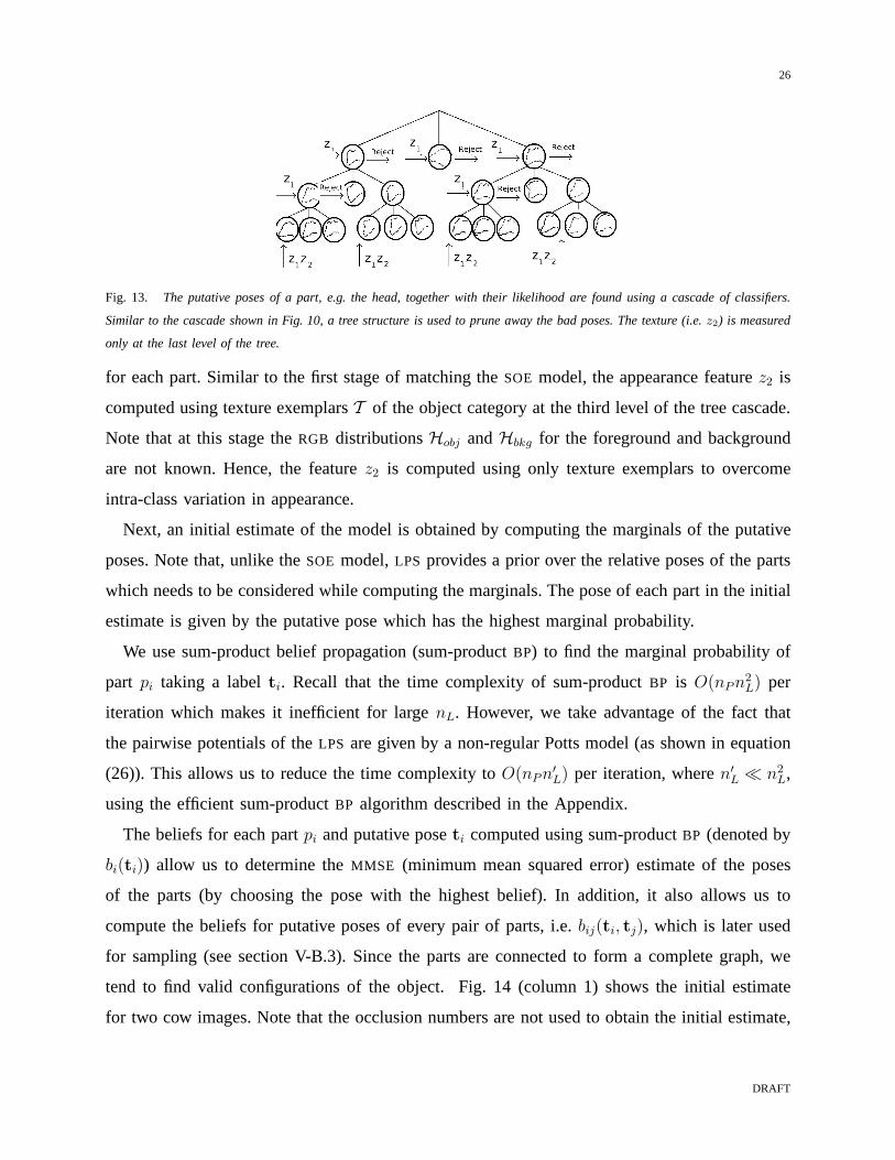
Fig. 13. The putative poses of a part, e.g. the head, together with their likelihood are found using a cascade of classifiers.
Similar to the cascade shown in Fig. 10, a tree structure is used to prune away the bad poses. The texture (i.e.z2) is measured
only at the last level of the tree.
for each part. Similar to the first stage of matching theSOE model, the appearance featurez2 is
computed using texture exemplarsT of the object category at the third level of the tree cascade.
Note that at this stage theRGB distributionsHobj andHbkg for the foreground and background
are not known. Hence, the featurez2 is computed using only texture exemplars to overcome
intra-class variation in appearance.
Next, an initial estimate of the model is obtained by computing the marginals of the putative
poses. Note that, unlike theSOE model,LPS provides a prior over the relative poses of the parts
which needs to be considered while computing the marginals.The pose of each part in the initial
estimate is given by the putative pose which has the highest marginal probability.
We use sum-product belief propagation (sum-productBP) to find the marginal probability of
part pi taking a labelti. Recall that the time complexity of sum-productBP is O(nPn2L) per
iteration which makes it inefficient for largenL. However, we take advantage of the fact that
the pairwise potentials of theLPS are given by a non-regular Potts model (as shown in equation
(26)). This allows us to reduce the time complexity toO(nPn′L) per iteration, wheren′
L ≪ n2L,
using the efficient sum-productBP algorithm described in the Appendix.
The beliefs for each partpi and putative poseti computed using sum-productBP (denoted by
bi(ti)) allow us to determine theMMSE (minimum mean squared error) estimate of the poses
of the parts (by choosing the pose with the highest belief). In addition, it also allows us to
compute the beliefs for putative poses of every pair of parts, i.e. bij(ti, tj), which is later used
for sampling (see section V-B.3). Since the parts are connected to form a complete graph, we
tend to find valid configurations of the object. Fig. 14 (column 1) shows the initial estimate
for two cow images. Note that the occlusion numbers are not used to obtain the initial estimate,
DRAFT
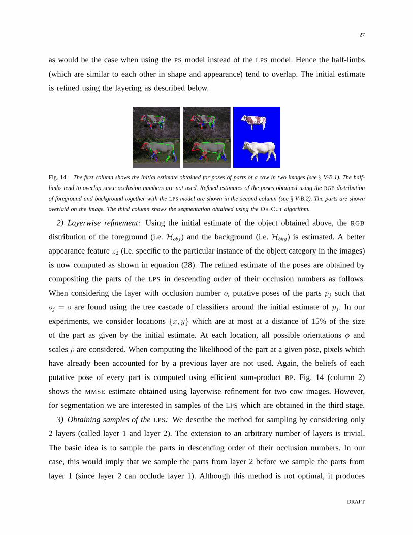
27
as would be the case when using thePS model instead of theLPS model. Hence the half-limbs
(which are similar to each other in shape and appearance) tend to overlap. The initial estimate
is refined using the layering as described below.
Fig. 14. The first column shows the initial estimate obtained for poses of parts of a cow in two images (see§ V-B.1). The half-
limbs tend to overlap since occlusion numbers are not used. Refined estimates of the poses obtained using theRGB distribution
of foreground and background together with theLPS model are shown in the second column (see§ V-B.2). The parts are shown
overlaid on the image. The third column shows the segmentation obtained using theOBJCUT algorithm.
2) Layerwise refinement:Using the initial estimate of the object obtained above, theRGB
distribution of the foreground (i.e.Hobj) and the background (i.e.Hbkg) is estimated. A better
appearance featurez2 (i.e. specific to the particular instance of the object category in the images)
is now computed as shown in equation (28). The refined estimate of the poses are obtained by
compositing the parts of theLPS in descending order of their occlusion numbers as follows.
When considering the layer with occlusion numbero, putative poses of the partspj such that
oj = o are found using the tree cascade of classifiers around the initial estimate ofpj. In our
experiments, we consider locationsx, y which are at most at a distance of 15% of the size
of the part as given by the initial estimate. At each location, all possible orientationsφ and
scalesρ are considered. When computing the likelihood of the part ata given pose, pixels which
have already been accounted for by a previous layer are not used. Again, the beliefs of each
putative pose of every part is computed using efficient sum-product BP. Fig. 14 (column 2)
shows theMMSE estimate obtained using layerwise refinement for two cow images. However,
for segmentation we are interested in samples of theLPS which are obtained in the third stage.
3) Obtaining samples of theLPS: We describe the method for sampling by considering only
2 layers (called layer 1 and layer 2). The extension to an arbitrary number of layers is trivial.
The basic idea is to sample the parts in descending order of their occlusion numbers. In our
case, this would imply that we sample the parts from layer 2 before we sample the parts from
layer 1 (since layer 2 can occlude layer 1). Although this method is not optimal, it produces
DRAFT

28
useful samples for segmentation in practice. To obtain a sample Ωi, parts belonging to layer 2
are considered first. The beliefs of these parts are computedusing efficient sum-productBP. The
posterior for sampleΩi is approximated as
g(Ωi|Z) =
∏
ij bij(ti, tj)∏
i bi(ti)qi−1, (29)
whereqi is the number of neighboring parts ofpi. Since we use a complete graph,qi = nP − 1,
for all partspi. Note that the posterior is exact only for a singly connectedgraph. However,
using this approximation sum-productBP has been shown to converge to stationary points of the
Bethe free energy [46].
The posterior is then sampled for poses, one part at a time (i.e. Gibbs sampling), such that the
pose of the part being sampled forms a valid configuration with the poses of the parts previously
sampled. The process is repeated to obtain multiple samplesΩi (which do not include the poses
of parts belonging to layer 1). This method of sampling is efficient since often very few pairs
of poses form a valid configuration. Further, these pairs arepre-computed during the efficient
sum-productBP algorithm as described in the Appendix. The bestnS samples, with the highest
belief, are chosen.
To obtain the poses of parts in layer 1 for sampleΩi, we fix the poses of parts belonging to
layer 2 as given byΩi. We calculate the posterior over the poses of parts in layer 1using sum-
productBP. We sample this posterior for poses of parts such that they form a valid configuration
with the poses of the parts in layer 2 and with those in layer 1 that were previously sampled.
As in the case of layer 2, multiple samples are obtained and the bestnS samples are chosen.
The process is repeated for all samplesΩi for layer 2, resulting in a total ofs = n2S samples.
However, computing the likelihood of the parts in layer 1 foreachΩ is expensive as their
overlap with parts in layer 2 needs to be considered. We use anapproximation by considering
only those poses whose overlap with layer 2 is below a threshold τ2. Fig. 15 shows some of the
samples obtained using the above method for the cows in Fig. 14.
Once the samples are obtained, they are used as inputs for theOBJCUT algorithm which
provides the segmentation. Note that the segmentation can then be used to obtain more accurate
samples (i.e. the generalizedEM algorithm can be iterated until convergence). However, we
observed that in almost all cases, the samples obtained in the second iteration (and hence, the
segmentation) did not differ significantly from the samplesin the first iteration (e.g. see Fig. 16).
DRAFT
29
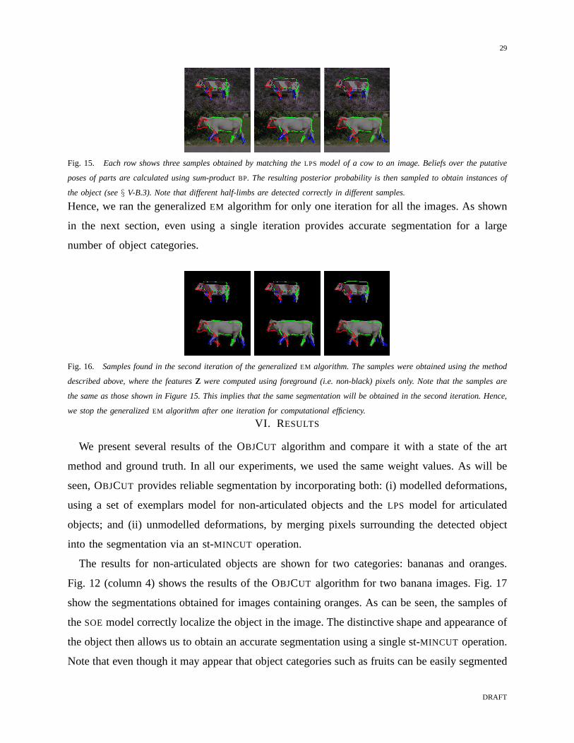
Fig. 15. Each row shows three samples obtained by matching theLPS model of a cow to an image. Beliefs over the putative
poses of parts are calculated using sum-productBP. The resulting posterior probability is then sampled to obtain instances of
the object (see§ V-B.3). Note that different half-limbs are detected correctly in different samples.
Hence, we ran the generalizedEM algorithm for only one iteration for all the images. As shown
in the next section, even using a single iteration provides accurate segmentation for a large
number of object categories.
Fig. 16. Samples found in the second iteration of the generalizedEM algorithm. The samples were obtained using the method
described above, where the featuresZ were computed using foreground (i.e. non-black) pixels only. Note that the samples are
the same as those shown in Figure 15. This implies that the same segmentation will be obtained in the second iteration. Hence,
we stop the generalizedEM algorithm after one iteration for computational efficiency.
VI. RESULTS
We present several results of the OBJCUT algorithm and compare it with a state of the art
method and ground truth. In all our experiments, we used the same weight values. As will be
seen, OBJCUT provides reliable segmentation by incorporating both: (i)modelled deformations,
using a set of exemplars model for non-articulated objects and the LPS model for articulated
objects; and (ii) unmodelled deformations, by merging pixels surrounding the detected object
into the segmentation via an st-MINCUT operation.
The results for non-articulated objects are shown for two categories: bananas and oranges.
Fig. 12 (column 4) shows the results of the OBJCUT algorithm for two banana images. Fig. 17
show the segmentations obtained for images containing oranges. As can be seen, the samples of
theSOE model correctly localize the object in the image. The distinctive shape and appearance of
the object then allows us to obtain an accurate segmentationusing a single st-MINCUT operation.
Note that even though it may appear that object categories such as fruits can be easily segmented
DRAFT
30
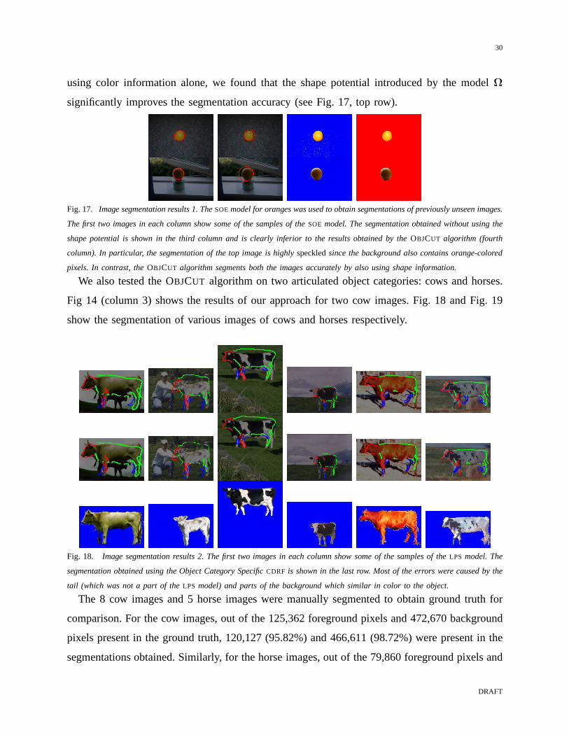
using color information alone, we found that the shape potential introduced by the modelΩ
significantly improves the segmentation accuracy (see Fig.17, top row).
Fig. 17. Image segmentation results 1. TheSOEmodel for oranges was used to obtain segmentations of previously unseen images.
The first two images in each column show some of the samples of the SOE model. The segmentation obtained without using the
shape potential is shown in the third column and is clearly inferior to the results obtained by theOBJCUT algorithm (fourth
column). In particular, the segmentation of the top image ishighly speckledsince the background also contains orange-colored
pixels. In contrast, theOBJCUT algorithm segments both the images accurately by also usingshape information.
We also tested the OBJCUT algorithm on two articulated object categories: cows and horses.
Fig 14 (column 3) shows the results of our approach for two cowimages. Fig. 18 and Fig. 19
show the segmentation of various images of cows and horses respectively.
Fig. 18. Image segmentation results 2. The first two images in each column show some of the samples of theLPS model. The
segmentation obtained using the Object Category SpecificCDRF is shown in the last row. Most of the errors were caused by the
tail (which was not a part of theLPS model) and parts of the background which similar in color to the object.
The 8 cow images and 5 horse images were manually segmented toobtain ground truth for
comparison. For the cow images, out of the 125,362 foreground pixels and 472,670 background
pixels present in the ground truth, 120,127 (95.82%) and 466,611 (98.72%) were present in the
segmentations obtained. Similarly, for the horse images, out of the 79,860 foreground pixels and
DRAFT
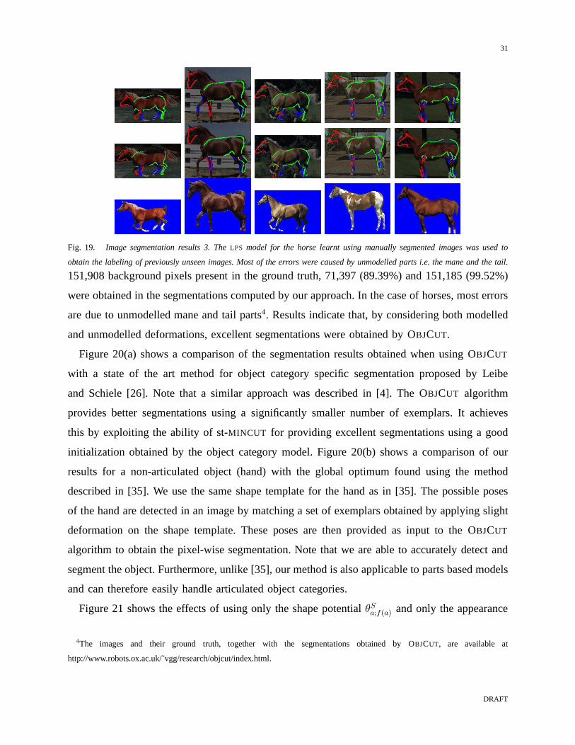
31
Fig. 19. Image segmentation results 3. TheLPS model for the horse learnt using manually segmented images was used to
obtain the labeling of previously unseen images. Most of theerrors were caused by unmodelled parts i.e. the mane and the tail.
151,908 background pixels present in the ground truth, 71,397 (89.39%) and 151,185 (99.52%)
were obtained in the segmentations computed by our approach. In the case of horses, most errors
are due to unmodelled mane and tail parts4. Results indicate that, by considering both modelled
and unmodelled deformations, excellent segmentations were obtained by OBJCUT.
Figure 20(a) shows a comparison of the segmentation resultsobtained when using OBJCUT
with a state of the art method for object category specific segmentation proposed by Leibe
and Schiele [26]. Note that a similar approach was describedin [4]. The OBJCUT algorithm
provides better segmentations using a significantly smaller number of exemplars. It achieves
this by exploiting the ability of st-MINCUT for providing excellent segmentations using a good
initialization obtained by the object category model. Figure 20(b) shows a comparison of our
results for a non-articulated object (hand) with the globaloptimum found using the method
described in [35]. We use the same shape template for the handas in [35]. The possible poses
of the hand are detected in an image by matching a set of exemplars obtained by applying slight
deformation on the shape template. These poses are then provided as input to the OBJCUT
algorithm to obtain the pixel-wise segmentation. Note thatwe are able to accurately detect and
segment the object. Furthermore, unlike [35], our method isalso applicable to parts based models
and can therefore easily handle articulated object categories.
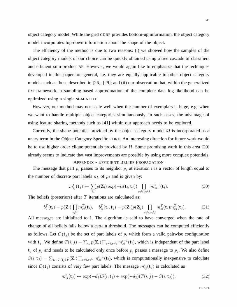
Figure 21 shows the effects of using only the shape potentialθSa;f(a) and only the appearance
4The images and their ground truth, together with the segmentations obtained by OBJCUT, are available at
http://www.robots.ox.ac.uk/˜vgg/research/objcut/index.html.
DRAFT
32
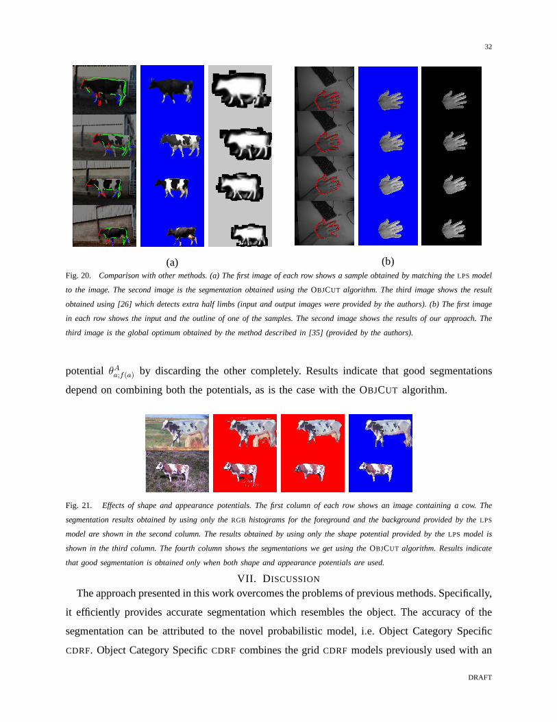
(a) (b)Fig. 20. Comparison with other methods. (a) The first image of each rowshows a sample obtained by matching theLPS model
to the image. The second image is the segmentation obtained using theOBJCUT algorithm. The third image shows the result
obtained using [26] which detects extra half limbs (input and output images were provided by the authors). (b) The first image
in each row shows the input and the outline of one of the samples. The second image shows the results of our approach. The
third image is the global optimum obtained by the method described in [35] (provided by the authors).
potential θAa;f(a) by discarding the other completely. Results indicate that good segmentations
depend on combining both the potentials, as is the case with the OBJCUT algorithm.
Fig. 21. Effects of shape and appearance potentials. The first columnof each row shows an image containing a cow. The
segmentation results obtained by using only theRGB histograms for the foreground and the background provided by the LPS
model are shown in the second column. The results obtained byusing only the shape potential provided by theLPS model is
shown in the third column. The fourth column shows the segmentations we get using theOBJCUT algorithm. Results indicate
that good segmentation is obtained only when both shape and appearance potentials are used.
VII. D ISCUSSION
The approach presented in this work overcomes the problems of previous methods. Specifically,
it efficiently provides accurate segmentation which resembles the object. The accuracy of the
segmentation can be attributed to the novel probabilistic model, i.e. Object Category Specific
CDRF. Object Category SpecificCDRF combines the gridCDRF models previously used with an
DRAFT
33
object category model. While the gridCDRF provides bottom-up information, the object category
model incorporates top-down information about the shape ofthe object.
The efficiency of the method is due to two reasons: (i) we showed how the samples of the
object category models of our choice can be quickly obtainedusing a tree cascade of classifiers
and efficient sum-productBP. However, we would again like to emphasize that the techniques
developed in this paper are general, i.e. they are equally applicable to other object category
models such as those described in [26], [29]; and (ii) our observation that, within the generalized
EM framework, a sampling-based approximation of the completedata log-likelihood can be
optimized using a single st-MINCUT.
However, our method may not scale well when the number of exemplars is huge, e.g. when
we want to handle multiple object categories simultaneously. In such cases, the advantage of
using feature sharing methods such as [41] within our approach needs to be explored.
Currently, the shape potential provided by the object category modelΩ is incorporated as a
unary term in the Object Category SpecificCDRF. An interesting direction for future work would
be to use higher order clique potentials provided byΩ. Some promising work in this area [20]
already seems to indicate that vast improvements are possible by using more complex potentials.
APPENDIX - EFFICIENT BELIEF PROPAGATION
The message that partpi passes to its neighborpj at iterationt is a vector of length equal to
the number of discrete part labelsnL of pj and is given by:
mtij(tj)←
∑
ti
p(Zi) exp(−α(ti, tj))∏
s 6=i,s 6=j
mt−1si (ti). (30)
The beliefs (posteriors) afterT iterations are calculated as:
bTi (ti) = p(Zi)
∏
s 6=i
mTsi(ti), bT
ij(ti, tj) = p(Zi)p(Zj)∏
s 6=i,s 6=j
mTsi(ti)m
Tsj(tj). (31)
All messages are initialized to1. The algorithm is said to have converged when the rate of
change of all beliefs falls below a certain threshold. The messages can be computed efficiently
as follows. LetCi(tj) be the set of part labels ofpi which form a valid pairwise configuration
with tj. We defineT (i, j) =∑
tip(Zi)
∏
s 6=i,s 6=j mt−1si (ti), which is independent of the part label
tj of pj and needs to be calculated only once beforepi passes a message topj. We also define
S(i, tj) =∑
ti∈Ci(tj) p(Zi)∏
s 6=i,s 6=j mt−1si (ti), which is computationally inexpensive to calculate
sinceCi(tj) consists of very few part labels. The messagemtij(tj) is calculated as
mtij(tj)← exp(−d1)S(i, tj) + exp(−d2)(T (i, j)− S(i, tj)). (32)
DRAFT

34
Clearly, the above message passing equation is equivalent to that shown in equation (30).
Acknowledgements.M. Pawan Kumar was funded by the EU CLASS project and by EPSRC grant
EP/C006631/1(P). Philip Torr is in receipt of a Royal Society Wolfson Research Merit Award,
and would like to acknowledge support from the Royal Societyand Wolfson foundation. Andrew
Zisserman thanks Microsoft Research and the Royal Academy of Engineering for support.
REFERENCES
[1] A. Agarwal and B. Triggs. Tracking articulated motion using a mixture of autoregressive models. InECCV, pages
III:54–65, 2004.
[2] A. Blake, C. Rother, M. Brown, P. Perez, and P.H.S. Torr. Interactive image segmentation using an adaptive GMMRF
model. InECCV, pages I: 428–441, 2004.
[3] A. Blake and A. Zisserman.Visual Reconstruction. MIT Press, 1987.
[4] E. Borenstein and S. Ullman. Class-specific, top-down segmentation. InECCV, page II: 109 ff., 2002.
[5] Y. Boykov and M.P. Jolly. Interactive graph cuts for optimal boundary and region segmentation of objects in N-D images.
In ICCV, pages I: 105–112, 2001.
[6] J.M. Coughlan, A.L. Yuille, C. English, and D. Snow. Efficient optimization of a deformable template using dynamic
programming. InCVPR, pages 747–752, 1998.
[7] D. Cremers, N. Sochen, and Schnoerr C. Mutliphase dynamic labelling for variational recognition-driven image
segmentation.IJCV, 66:67–81, 2006.
[8] P.F. Felzenszwalb. Representation and detection of deformable shapes. InCVPR, pages I: 102–108, 2003.
[9] P.F. Felzenszwalb and D.P. Huttenlocher. Efficient matching of pictorial structures. InCVPR, pages II: 66–73, 2000.
[10] P.F. Felzenszwalb and D.P. Huttenlocher. Fast algorithms for large state space HMMs with applications to web usage
analysis. InNIPS, 2003.
[11] R. Fergus, P. Perona, and A. Zisserman. Object class recognition by unsupervised scale-invariant learning. InCVPR, pages
II: 264–271, 2003.
[12] M.A. Fischler and R.A. Elschlager. The representationand matching of pictorial structures.TC, 22:67–92, January 1973.
[13] D. Freedman and T. Zhang. Interactive graph cut based segmentation with shape priors. InCVPR, pages I: 755–762, 2005.
[14] D.M. Gavrilla. Pedestrian detection from a moving vehicle. In ECCV, pages II: 37–49, 2000.
[15] A. Gelman, J. Carlin, H. Stern, and D. Rubin.Bayesian Data Analysis. Chapman and Hall, 1995.
[16] S. Geman and D. Geman. Stochastic relaxation, gibbs distributions, and the bayesian restoration of images.PAMI,
6(6):721–741, 1984.
[17] J. Goldstein, J. Platt, and C. Burges. Redundant bit vectors for quickly searching high-dimensional regions. InDeterministic
and Statistical Methods in Machine Learning, pages 137–158, 2005.
[18] P. Hammer. Some network flow problems solved with pseudo-boolean programming.Operations Research, 13:388–399,
1965.
[19] R. Huang, V. Pavlovic, and D.N. Metaxas. A graphical model framework for coupling MRFs and deformable models. In
CVPR, pages II: 739–746, 2004.
[20] P. Kohli, M. P. Kumar, and P. H. S. Torr. P3 & beyond: Solving energies with higher order cliques. InCVPR, 2007.
[21] V. Kolmogorov and R. Zabih. What energy functions can beminimized via graph cuts.IEEE PAMI, 26(2):147–159, 2004.
DRAFT
35
[22] M. P. Kumar, P. H. S. Torr, and A. Zisserman. Extending pictorial structures for object recognition. InBMVC, pages II:
789–798, 2004.
[23] M. P. Kumar, P. H. S. Torr, and A. Zisserman. OBJ CUT. In CVPR, pages I: 18–25, 2005.
[24] M. P. Kumar, P. H. S. Torr, and A. Zisserman. Learning layered motion segmentations of video.International Journal of
Computer Vision, 76(3):301–319, 2008.
[25] J. Lafferty, A. McCallum, and F. Pereira. Conditional random fields: Probabilistic models for segmenting and labelling
sequence data. InICML, 2001.
[26] B. Leibe and B. Schiele. Interleaved object categorization and segmentation. InBMVC, pages II: 264–271, 2003.
[27] A. Levin and Y. Weiss. Learning to combine bottom-up andtop-down segmentation. InECCV, pages IV: 581–594, 2006.
[28] P. Meer and B. Georgescu. Edge detection with embedded confidence.PAMI, 23:1351–1365, December 2001.
[29] A. Opelt, A. Pinz, and A. Zisserman. Incremental learning of object detectors using a visual shape alphabet. InCVPR,
pages I: 3–10, 2006.
[30] M. Prasad, A. Zisserman, A. Fitzgibbon, M. P. Kumar and P. H. S. Torr. Learning class-specific edges for object detection
and segmentation. InICVGIP, 2006.
[31] D. Ramanan. Using segmentation to verify object hypothesis. InCVPR, 2007.
[32] D. Ramanan and D.A. Forsyth. Using temporal coherence to build models of animals. InICCV, pages 338–345, 2003.
[33] J. Rihan, P. Kohli, and P. H. S. Torr. OBJCUT for face detection. In ICVGIP, 2006.
[34] C. Rother, V. Kolmogorov, and A. Blake. Grabcut: interactive foreground extraction using iterated graph cuts. In
SIGGRAPH, pages 309–314, 2004.
[35] T. Schoenemann and D. Cremers. Globally optimal image segmentation with an elastic shape prior. InICCV, 2007.
[36] T. Schoenemann and D. Cremers. Globally optimal shape-based tracking in real-time. InCVPR, 2008.
[37] J. Shotton, A. Blake, and R. Cipolla. Contour-based learning for object detection. InICCV, pages I: 503–510, 2005.
[38] J. Shotton, J. Winn, C. Rother, and A. Criminisi. TextonBoost: Joint appearance, shape and context modeling for multi-class
object recognition and segmentation. InECCV, pages I: 1–15, 2006.
[39] B. Stenger, A. Thayananthan, P.H.S. Torr, and R. Cipolla. Hand pose estimation using heirarchical detection. InIntl.
Workshop on Human-Computer Interaction, pages 105–116, 2004.
[40] A. Thayananthan, B. Stenger, P.H.S. Torr, and R. Cipolla. Shape context and chamfer matching in cluttered scenes. In
CVPR, pages I: 127–133, 2003.
[41] A. Torralba, K.P. Murphy, and W.T. Freeman. Sharing visual features for multiclass and multiview object detection. PAMI,
29(5):854–869, 2007.
[42] K. Toyama and A. Blake. Probabilistic tracking in a metric space. InICCV, pages II: 50–57, 2001.
[43] M. Varma and A. Zisserman. Texture classification: Are filter banks necessary? InCVPR, pages II:691–698, 2003.
[44] J. Winn and N. Jojic. LOCUS: Learning Object Classes with Unsupervised Segmentation. InICCV, pages I: 756–763,
2005.
[45] J. Winn and J. Shotton. The layout consistent random field for recognizing and segmenting partially occluded objects. In
CVPR, pages I: 37–44, 2006.
[46] J. Yedidia, W. Freeman, and Y. Weiss. Bethe free energy,kikuchi approximations, and belief propagation algorithms.
Technical Report TR2001-16, MERL, 2001.
DRAFT


![Cell Segmentation: 50 Years Down the · PDF fileCell Segmentation: 50 Years Down the Road ... processing, and analysis. Consequently, comput- ... in cell biology [3–6]](https://img.pdfslide.net/doc/110x75/5aa26a647f8b9ab4208d048b/cell-segmentation-50-years-down-the-segmentation-50-years-down-the-road-processing.jpg)
![OBJCUT: Efficient Segmentation Using Top-Down and Bottom ...vgg/publications/papers/kumar10.pdf · a patch-based model learned from training images. Leibe and Schiele [26] provide](https://img.pdfslide.net/doc/110x75/5f80010727b65b04736143ad/objcut-efficient-segmentation-using-top-down-and-bottom-vggpublicationspaperskumar10pdf.jpg)