Object Segmentation in Video: A Hierarchical Variational Approach for TurningPoint Trajectories into Dense Regions

Peter Ochs and Thomas BroxComputer Vision Group

University of Freiburg, Germanyochs, brox@informatik.uni-freiburg.de

Abstract

Point trajectories have emerged as a powerful means toobtain high quality and fully unsupervised segmentation ofobjects in video shots. They can exploit the long term mo-tion difference between objects, but they tend to be sparsedue to computational reasons and the difficulty in estimat-ing motion in homogeneous areas. In this paper we intro-duce a variational method to obtain dense segmentationsfrom such sparse trajectory clusters. Information is propa-gated with a hierarchical, nonlinear diffusion process thatruns in the continuous domain but takes superpixels into ac-count. We show that this process raises the density from 3%to 100% and even increases the average precision of labels.

1. Introduction

Current learning frameworks for visual recognition relyon manual annotation including manual segmentation of ob-jects. Taking the best vision system solution to-date – thehuman brain – such annotation should not be necessary. In-fants learn the visual appearance and shape of objects with-out being provided bounding boxes and segmentations bytheir parents. There is convincing evidence that infants ob-tain such object segmentations via motion cues [22, 17] andone could argue that computational vision systems shouldfinally work in a similar way.

Motion analysis of point trajectories is a reasonably ro-bust tool to extract object regions from video shots in afully unsupervised manner, as recently demonstrated, e.g.,in [20, 7]. However, these approaches have to struggle withthe fact that motion estimation requires structures to match.In homogeneous areas of the image there are no such struc-tures. This results in point trajectories to be sparse. Al-though the work in [7] is based on point trajectories derivedfrom dense optical flow and the obtained trajectories couldbe made dense, trajectories in homogenous areas are less

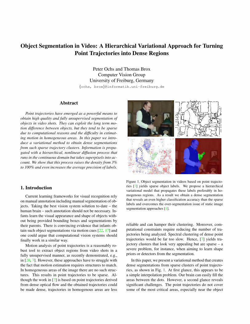
Figure 1. Object segmentation in videos based on point trajecto-ries [7] yields sparse object labels. We propose a hierarchicalvariational model that propagates these labels preferably in ho-mogenous regions. As a result we obtain a dense segmentationthat reveals an even higher classification accuracy than the sparselabels and overcomes the over-segmentation issue of static imagesegmentation approaches [1].

reliable and can hamper their clustering. Moreover, com-putational constraints require reducing the number of tra-jectories being analyzed. Spectral clustering of dense pointtrajectories would be far too slow. Hence, [7] yields tra-jectory clusters that look very appealing but are sparse – asevere problem, for instance, when aiming to learn shapepriors or detectors from the segmentation.

In this paper, we present a variational method that createsdense segmentations from sparse clusters of point trajecto-ries, as shown in Fig. 1. At first glance, this appears to bea simple interpolation problem. Our brain can easily fill theareas between the dots. However, a second glance revealssignificant challenges. The point trajectories do not coversome of the most critical areas, especially near the object

boundaries. Those trajectories that exist near object bound-aries are often assigned wrong labels because the underly-ing optical flow is imprecise in occlusion areas. Finally, inlarge homogeneous areas there is hardly any label informa-tion.

For a good label propagation, the key is to exploit colorand edge information, which is complementary to the infor-mation used for generating the trajectory labels. Notably,segmentation based on color works the best in homoge-neous areas, which are the problematic areas for motionbased segmentation. We achieve this by spreading infor-mation depending on color homogeneity. To this end, wepropose a hierarchical variational model, where we havecontinuous labeling functions on multiple levels. Each levelcorresponds to a superpixel partitioning at a certain granu-larity level. In contrast to a single-level model we have ad-ditional auxiliary functions at coarser levels which are op-timized in a coupled diffusion process. To the best of ourknowledge, this is the first continuous hierarchical model.The advantage of such an approach is that we obtain astructure-aware label propagation thanks to the superpixelhierarchy, while the final solution can be extracted at thefinest level and is free of metrication errors or block arti-facts known from discrete MRF models.

2. Related workThe problem we consider here is related to interactive

segmentation, where the user draws a few scribbles intothe image and the approach propagates these labels to thenon-marked areas. Several techniques based on graph cuts[4], random walks [12], and intermediate settings [21] havebeen proposed. The latest techniques are built upon vari-ational convex relaxation methods [23, 18, 14, 16], whichavoid the discretization artifacts typical for classical MRFsdefined on a graph. The variational technique we proposehere in fact builds on the regularizer from [14].

None of these approaches consider a hierarchy. More-over, labels from point trajectories differ from user scribblesin two ways. First, the labels are generated by an unsuper-vised approach and are likely to be erroneous, whereas in-teractive segmentation relies on the correctness of the user’sinput. This means, we do not have an interpolation but anapproximation problem. For this reason, we do not fol-low the typical approach of estimating appearance statisticsfrom the annotated areas combined with a typical regionbased segmentation. We rather formulate the problem asa label diffusion problem, where diffusion takes place onvarious hierarchy levels. Second, user annotation providesdense finite annotation areas, whereas trajectory labels con-stitute single points spread over the image. It is not imme-diate that a variational model acting on such infinitesimallysmall labels makes sense in the continuous limit. We showthat our continuous model satisfies certain regularity prop-

erties and thus is a proper continuous formulation of theproblem.

Our model is also related to image compression withanisotropic diffusion [11], where only a small set of pixelvalues is kept and the original image is sought to be restoredby running a diffusion process on this sparse representation.

On the task of dense motion segmentation, there aremany recent works that produce over-segmentations usingsuperpixels, label propagation by optical flow, or other clus-tering methods [5, 13, 24, 15]. These over-segmentationsdo not provide object regions. User interactive video seg-mentation methods can avoid over-segmentation, but are nolonger unsupervised [3, 19].

3. Single-level variational modelGiven a video shot as input, we apply the clustering ap-

proach on point trajectories using the code from [7]. Thisyields a discrete sparse set of labels, which are consistentover the whole shot. Fig. 1 shows an example frame and thelabels obtained with [7]. Approximately 3% of the pixelsare labeled.

Let u := (u1, . . . , un) : Ω → 0, 1n, n ∈ N be a func-tion indicating the n different point trajectory labels, i.e.,

ui :=

1, if x ∈ Li

0, else,(1)

where Li is the set of coordinates occupied by a trajectorywith label i and Ω ⊂ R2 denotes the image domain. Forsimplicity, we focus on single images, although our modelcould be easily extended to compute a temporally consistentsolution for all images of the video.

We seek a function u := (u1, . . . , un) : Ω → 0, 1nthat stays close to the given labels for points in L :=⋃n

i=1 Li. This is achieved by minimizing the energy

Edata(u) :=1

2

∫Ω

c

n∑i=1

(ui − ui)2dx, (2)

where c : Ω→ 0, 1 is the label indicator function, a char-acteristic function with value 1 on L and 0 else.

The above energy puts constraints only on points occu-pied by trajectories. On all other points, the minimizer cantake any value. To force these points to take specific labels,we require a regularizer

Ereg(u) :=

∫Ω

g ψ

(n∑

i=1

|∇BVui|2)dx, (3)

which is chosen such that it prefers compact regions withminimal perimeter and such that labels are propagatedpreferably in homogenous areas. The first is achieved bythe regularized TV norm obtained with ψ(s2) :=

√s2 + ε2

and ε := 0.001, the second by the diffusivity functiong : Ω→ R+

g(|∇I(x)|2) :=1√

|∇I(x)|2 + ε2. (4)

Since ui is binary-valued, it lies in the space of functionsof bounded variation BV(Ω), which includes functions withsharp discontinuities [2]. The ordinary gradient operator ∇is not defined for such functions. Thus, we replace it by∇BV , which is the distributional derivative and is definedalso for characteristic functions. In case of continuous func-tions ∇BV ≡ ∇.

Convex combination of the energies in (2) and (3) yields

E(u) :=α

2

∫Ω

c

n∑i=1

(ui − ui)2 dx

+ (1− α)

∫Ω

g ψ

(n∑

i=1

|∇BVui|2)dx

(5)

s.t.∑

i ui(x) = 1, ∀x with a model parameter α ∈ [0, 1)that can be chosen depending on the credibility of the tra-jectory labels. In the limit α → 1, the minimizer will bean interpolation, otherwise it is an approximation that cancorrect erroneous labels.

3.1. Minimization

The functions ui are binary-valued. For we can applyvariational methods we must consider the relaxed problem,where we allow ui to take values in the interval [0, 1]. Suchrelaxations have been suggested for many similar problems[8, 18, 14]. Since both the energy and the relaxed feasibleset are convex, we find the global minimizer of the relaxedproblem. Except for the two-label setting in [8], project-ing this minimizer back to the original feasible set gener-ally does not ensure the global optimum but yields a goodapproximation.

For the relaxed problem, we may assume that u is con-tinuous differentiable, so we may replace ∇BV by ∇. TheEuler-Lagrange equations of the relaxed energy reads

0 = α c · (ui − ui)

− (1− α) div

(g ψ′

(n∑

i=1

|∇ui|2)∇ui

)∀i.

(6)

We solve this nonlinear system with a fixed point iterationscheme, where the nonlinear factor ψ′(s2) = (s2+ε2)−

12 is

kept constant in each iteration. The resulting linear systemis solved with successive over-relaxation (SOR). The con-straint

∑i ui(x) = 1, ∀x is enforced in each fixed point

iteration by normalization as proposed in [9]. The obtainedrelaxed result is projected to 0, 1n via

ui(x) =

1, if i = argmaxiui|i = 1, ..., n0, else.

(7)

3.2. Model consistency

It can be argued that c and u, as indicator functions,differ from 1 only on a discrete set, i.e., on a null-set.Following the theory of Lebesgue measures, the energyEdata ≡ 0. This problem can be avoided by a minor adap-tion of the model. Replace c by its C∞-approximationcε ∈ C∞(Ω, [0, 1]) satisfying cε → c as ε → 0 and themass conservation

∫Bε(x)

cε(x)dx = 1, where Bε(x) de-notes the ball with radius ε at x, e.g.,

cε(x) :=∑x∈L

δε(x− x). (8)

Define uε analogously as such an approximation to u. Notethat the mappings cε and uε are well-defined as mappingswith range [0, 1] and [0, 1]n, respectively. The assumptionof a discrete set of input labels assures non-overlappingε-neighborhoods, and thus implies the well-definedness.Choosing ε > 0 small enough to satisfy this separationproperty for all x ∈ L yields the consistent regularised en-ergy Edata,ε by replacing c and u by cε and uε in (2). Weomit the ε due to notational simplicity.

4. Multi-level variational modelThe Euler-Lagrange equations in (6) can be interpreted

as a nonlinear diffusion process subject to the constraint thatthe points in L should stay close to their original label u.These points serve as sources for spreading their respectivelabel information. The antipoles that consume this labelmass are other labels in the neighborhood. Depending onhow much label mass is consumed by neighboring pointsand depending on α, a source point x ∈ L can also changeits label in the final solution u, but it still remains a sourceof the original label’s mass.

Especially in homogeneous areas, the density of sourcepoints is low, i.e., the information must be propagated overlarge spatial distances, damped by noise and unimportantstructures. To overcome this problem, we propose a hierar-chical model. The finest level in this hierarchy correspondsto the single-level model we have introduced in the previoussection. Additional levels make use of superpixels obtainedwith the approach from [1]. Fig. 2a illustrates the contin-uous hierarchy. Fig. 2b shows the corresponding discretegraph structure for helping readers who prefer to think indiscrete terms.

Each level k, k = 0, ...,K, in our variational model rep-resents a continuous function that is partitioned into Mk

superpixels Ωkm,m = 1, ...,Mk. For k = 0 we have the

functions u0 and I0 as defined for the single-level model.For k > 0 we have the corresponding piecewise constantfunctions uk and Ik, where Ik(x) = 1

|Ωkm|∫

ΩkmI0(x′)dx′

takes the mean color of the corresponding superpixel Ωkm.

The idea behind these additional auxiliary functions at

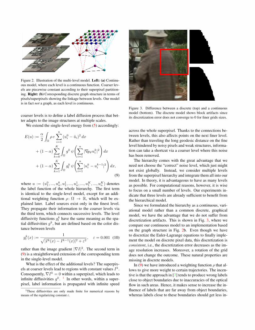
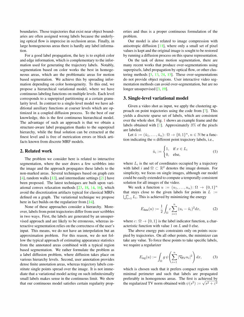
Figure 2. Illustration of the multi-level model. Left: (a) Continu-ous model, where each level is a continuous function. Coarser lev-els are piecewise constant according to their superpixel partition-ing. Right: (b) Corresponding discrete graph structure in terms ofpixels/superpixels showing the linkage between levels. Our modelis in fact not a graph, as each level is continuous.

coarser levels is to define a label diffusion process that bet-ter adapts to the image structures at multiple scales.

We extend the single-level energy from (5) accordingly:

E(u) :=α

2

∫Ω

ρ c

n∑i=1

(u0i − ui)2 dx

+ (1− α)

K∑k=0

∫Ω

gk ψ

(n∑

i=1

|∇BVuki |2)dx

+ (1− α)

K∑k=1

∫Ω

gkl ψ

(n∑

i=1

|uki − uk−1i |2

)dx,

(9)

where u := (u01, ..., u

0n, u

11, ..., u

1n, ..., u

K1 , ..., u

Kn ) denotes

the label function of the whole hierarchy. The first termis identical to the single-level model, except for an addi-tional weighting function ρ : Ω → R, which will be ex-plained later. Label sources exist only in the finest level.They propagate their information to the coarser levels viathe third term, which connects successive levels. The leveldiffusivity functions gkl have the same meaning as the spa-tial diffusivities gk, but are defined based on the color dis-tance between levels

gkl (x) :=1√

|Ik(x)− Ik−1(x)|2 + ε2, ε = 0.001 (10)

rather than the image gradient |∇I|2. The second term in(9) is a straightforward extension of the corresponding termin the single-level model.

What is the effect of the additional levels? The superpix-els at coarser levels lead to regions with constant values Ik.Consequently,∇Ik = 0 within a superpixel, which leads toinfinite diffusivities gk. 1 In other words, within a super-pixel, label information is propagated with infinite speed

1These diffusivities are only made finite for numerical reasons bymeans of the regularizing constant ε.

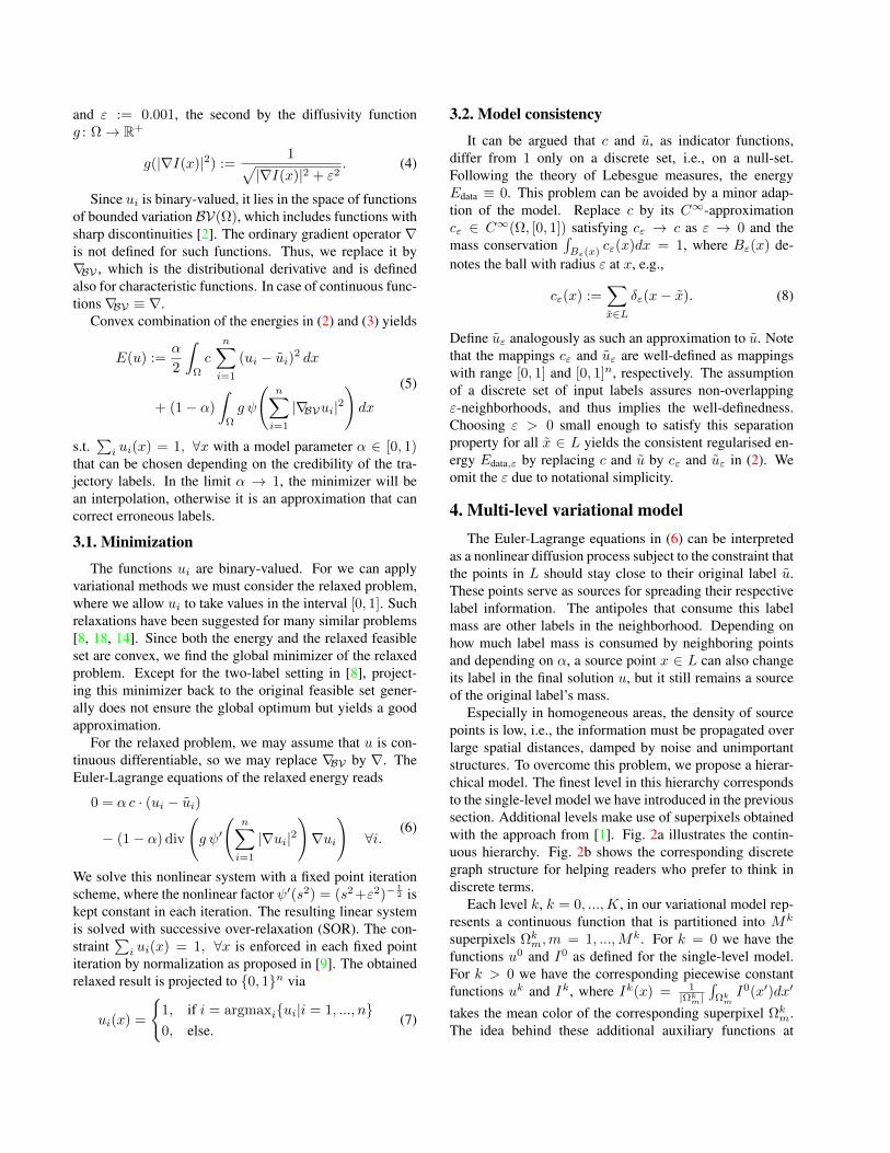
Figure 3. Difference between a discrete (top) and a continuousmodel (bottom). The discrete model shows block artifacts sinceits discretization error does not converge to 0 for finer grids sizes.

across the whole superpixel. Thanks to the connections be-tween levels, this also affects points on the next finer level.Rather than traveling the long geodesic distance on the finelevel hindered by noisy pixels and weak structures, informa-tion can take a shortcut via a coarser level where this noisehas been removed.

The hierarchy comes with the great advantage that weneed not choose the “correct” noise level, which just mightnot exist globally. Instead, we consider multiple levelsfrom the superpixel hierarchy and integrate them all into ourmodel. In theory, it is advantageous to have as many levelsas possible. For computational reasons, however, it is wiseto focus on a small number of levels. Our experiments in-dicate that three levels are already sufficient to benefit fromthe hierarchical model.

Since we formulated the hierarchy as a continuous, vari-ational model rather than a common discrete, graphicalmodel, we have the advantage that we do not suffer fromdiscretization artifacts. This is shown in Fig. 3, where wecompare our continuous model to an implementation basedon the graph structure in Fig. 2b. Even though we haveto discretize the Euler-Lagrange equations to finally imple-ment the model on discrete pixel data, this discretization isconsistent, i.e., the discretization error decreases as the im-age resolution increases. Moreover, a rotation of the griddoes not change the outcome. These natural properties aremissing in discrete models.

In (9) we have introduced a weighting function ρ that al-lows to give more weight to certain trajectories. The incen-tive is that the approach in [7] tends to produce wrong labelsclose to object boundaries due to inaccuracies of the opticalflow in such areas. Hence, it makes sense to increase the in-fluence of labels that are far away from object boundaries,whereas labels close to these boundaries should get less in-

Figure 4. Evolution of the label functions uk1 on all three levels simultaneously. Intermediate states after 30, 300, 3000, and 30000 iterations

are shown. For this visualization we did not use the cascadic multigrid strategy, which requires far fewer iterations to converge.

fluence. Since we do not yet know the object boundaries,the distance is approximated by the Euclidean distance tothe superpixel boundaries ∂Ωm at the coarsest level, whichcan be computed very efficiently [10]. Based on these dis-tances we define

ρ(x) :=dist(x, ∂Ωm)

1|Ωm|

∑x∈Ωm

dist(x, ∂Ωm)(11)

with x ∈ Ωm. This includes a normalization of the dis-tance by the size and shape of the superpixel. In large ho-mogenous regions, where optical flow estimation is mostproblematic, ρ increases slowly with the distance. In smallsuperpixels, indicating textured areas, even points close tothe boundary are assigned large weights.

4.1. MinimizationMinimization of the multi-level model is very similar to

the single-level model. The Euler-Lagrange equations of (9)for the levels k > 0 read

Dki := −div

(gk ψ′

(n∑

i=1

|∇uki |2)∇uk

i

)

+

(gkl ψ

′

(n∑

i=1

|uki − uk−1

i |2)|uk

i − uk−1i |

)

−

(gk+1l ψ′

(n∑

i=1

|uk+1i − uk

i |2)|uk+1

i − uki |

)= 0

(12)for all i = 1, . . . , n, stating a nonlinear system with vari-ables on multiple levels. Using this term and the Neumann

boundary conditions u−1i = u0

i and uK+1i = uKi for all i,

the Euler-Lagrange equations for k = 0 read

0 = αρ c ·(u0i − ui

)+ (1− α)D0

i . (13)

Again we apply fixed point iterations together with SOR.Intermediate states of the iterative method are shown inFig. 4.

4.2. Implementation details

As labels within a superpixel are propagated with infinitespeed, we can approximate the whole superpixel by a sin-gle constant value. Treating each superpixel as a single gridpoint, this leads to a considerable speedup as coarse levelsconsist of only few superpixels. In order to keep the advan-tages of the continuous model, the length of the interfacebetween two superpixels and their diffusivity must be mea-sured in a consistent manner using a properly discretizedgradient operator. Such a discretization can be found, e.g.,in [6, pp. 16].

At coarser levels, we further add non-local superpixelneighbors. These enable labels to cross obstacle regions thathave a significantly different color, for instance the shadowin Fig. 7. We connect all superpixels that are separated byonly one further superpixel. Since there is no direct inter-face that would define the amount of diffusion between twosuperpixels, we weight non-local diffusivities by the dis-tance between the segments using a Gaussian function

wab := exp

(−dist

2(a, b)

2σ2

)(14)

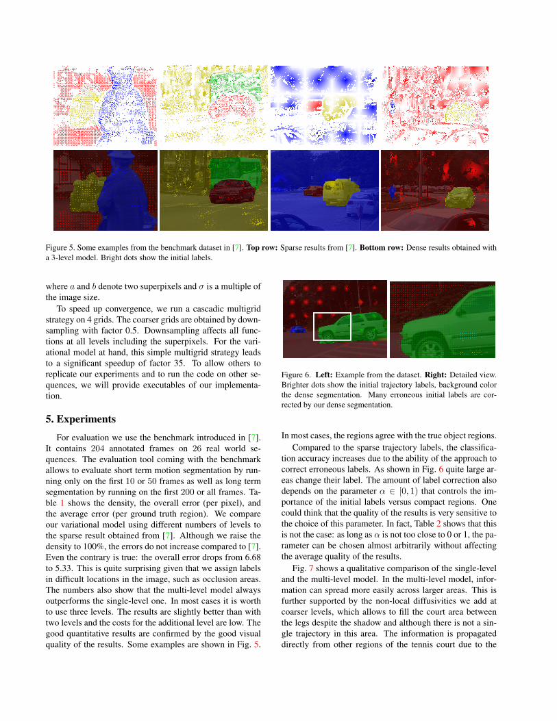
Figure 5. Some examples from the benchmark dataset in [7]. Top row: Sparse results from [7]. Bottom row: Dense results obtained witha 3-level model. Bright dots show the initial labels.

where a and b denote two superpixels and σ is a multiple ofthe image size.

To speed up convergence, we run a cascadic multigridstrategy on 4 grids. The coarser grids are obtained by down-sampling with factor 0.5. Downsampling affects all func-tions at all levels including the superpixels. For the vari-ational model at hand, this simple multigrid strategy leadsto a significant speedup of factor 35. To allow others toreplicate our experiments and to run the code on other se-quences, we will provide executables of our implementa-tion.

5. Experiments

For evaluation we use the benchmark introduced in [7].It contains 204 annotated frames on 26 real world se-quences. The evaluation tool coming with the benchmarkallows to evaluate short term motion segmentation by run-ning only on the first 10 or 50 frames as well as long termsegmentation by running on the first 200 or all frames. Ta-ble 1 shows the density, the overall error (per pixel), andthe average error (per ground truth region). We compareour variational model using different numbers of levels tothe sparse result obtained from [7]. Although we raise thedensity to 100%, the errors do not increase compared to [7].Even the contrary is true: the overall error drops from 6.68to 5.33. This is quite surprising given that we assign labelsin difficult locations in the image, such as occlusion areas.The numbers also show that the multi-level model alwaysoutperforms the single-level one. In most cases it is worthto use three levels. The results are slightly better than withtwo levels and the costs for the additional level are low. Thegood quantitative results are confirmed by the good visualquality of the results. Some examples are shown in Fig. 5.

Figure 6. Left: Example from the dataset. Right: Detailed view.Brighter dots show the initial trajectory labels, background colorthe dense segmentation. Many erroneous initial labels are cor-rected by our dense segmentation.

In most cases, the regions agree with the true object regions.Compared to the sparse trajectory labels, the classifica-

tion accuracy increases due to the ability of the approach tocorrect erroneous labels. As shown in Fig. 6 quite large ar-eas change their label. The amount of label correction alsodepends on the parameter α ∈ [0, 1) that controls the im-portance of the initial labels versus compact regions. Onecould think that the quality of the results is very sensitive tothe choice of this parameter. In fact, Table 2 shows that thisis not the case: as long as α is not too close to 0 or 1, the pa-rameter can be chosen almost arbitrarily without affectingthe average quality of the results.

Fig. 7 shows a qualitative comparison of the single-leveland the multi-level model. In the multi-level model, infor-mation can spread more easily across larger areas. This isfurther supported by the non-local diffusivities we add atcoarser levels, which allows to fill the court area betweenthe legs despite the shadow and although there is not a sin-gle trajectory in this area. The information is propagateddirectly from other regions of the tennis court due to the

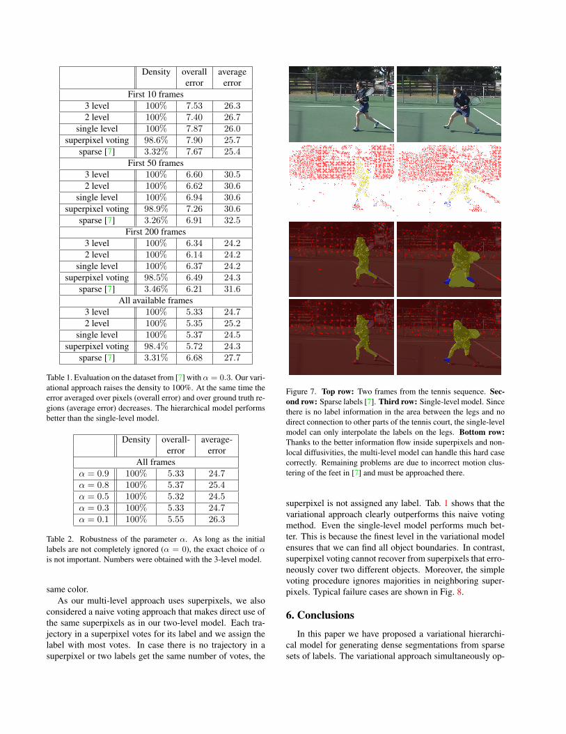
Density overall averageerror error

First 10 frames3 level 100% 7.53 26.32 level 100% 7.40 26.7

single level 100% 7.87 26.0superpixel voting 98.6% 7.90 25.7

sparse [7] 3.32% 7.67 25.4First 50 frames

3 level 100% 6.60 30.52 level 100% 6.62 30.6

single level 100% 6.94 30.6superpixel voting 98.9% 7.26 30.6

sparse [7] 3.26% 6.91 32.5First 200 frames

3 level 100% 6.34 24.22 level 100% 6.14 24.2

single level 100% 6.37 24.2superpixel voting 98.5% 6.49 24.3

sparse [7] 3.46% 6.21 31.6All available frames

3 level 100% 5.33 24.72 level 100% 5.35 25.2

single level 100% 5.37 24.5superpixel voting 98.4% 5.72 24.3

sparse [7] 3.31% 6.68 27.7

Table 1. Evaluation on the dataset from [7] withα = 0.3. Our vari-ational approach raises the density to 100%. At the same time theerror averaged over pixels (overall error) and over ground truth re-gions (average error) decreases. The hierarchical model performsbetter than the single-level model.

Density overall- average-error error

All framesα = 0.9 100% 5.33 24.7α = 0.8 100% 5.37 25.4α = 0.5 100% 5.32 24.5α = 0.3 100% 5.33 24.7α = 0.1 100% 5.55 26.3

Table 2. Robustness of the parameter α. As long as the initiallabels are not completely ignored (α = 0), the exact choice of αis not important. Numbers were obtained with the 3-level model.

same color.As our multi-level approach uses superpixels, we also

considered a naive voting approach that makes direct use ofthe same superpixels as in our two-level model. Each tra-jectory in a superpixel votes for its label and we assign thelabel with most votes. In case there is no trajectory in asuperpixel or two labels get the same number of votes, the

Figure 7. Top row: Two frames from the tennis sequence. Sec-ond row: Sparse labels [7]. Third row: Single-level model. Sincethere is no label information in the area between the legs and nodirect connection to other parts of the tennis court, the single-levelmodel can only interpolate the labels on the legs. Bottom row:Thanks to the better information flow inside superpixels and non-local diffusivities, the multi-level model can handle this hard casecorrectly. Remaining problems are due to incorrect motion clus-tering of the feet in [7] and must be approached there.

superpixel is not assigned any label. Tab. 1 shows that thevariational approach clearly outperforms this naive votingmethod. Even the single-level model performs much bet-ter. This is because the finest level in the variational modelensures that we can find all object boundaries. In contrast,superpixel voting cannot recover from superpixels that erro-neously cover two different objects. Moreover, the simplevoting procedure ignores majorities in neighboring super-pixels. Typical failure cases are shown in Fig. 8.

6. Conclusions

In this paper we have proposed a variational hierarchi-cal model for generating dense segmentations from sparsesets of labels. The variational approach simultaneously op-

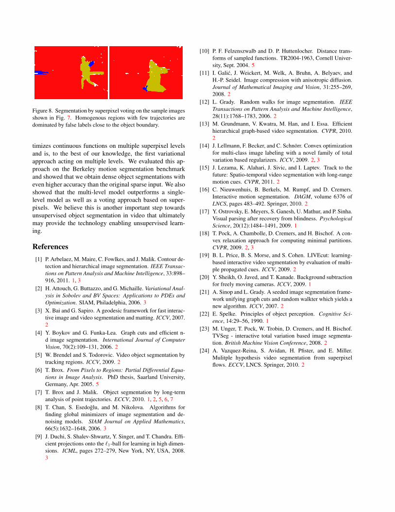
Figure 8. Segmentation by superpixel voting on the sample imagesshown in Fig. 7. Homogenous regions with few trajectories aredominated by false labels close to the object boundary.

timizes continuous functions on multiple superpixel levelsand is, to the best of our knowledge, the first variationalapproach acting on multiple levels. We evaluated this ap-proach on the Berkeley motion segmentation benchmarkand showed that we obtain dense object segmentations witheven higher accuracy than the original sparse input. We alsoshowed that the multi-level model outperforms a single-level model as well as a voting approach based on super-pixels. We believe this is another important step towardsunsupervised object segmentation in video that ultimatelymay provide the technology enabling unsupervised learn-ing.

References[1] P. Arbelaez, M. Maire, C. Fowlkes, and J. Malik. Contour de-

tection and hierarchical image segmentation. IEEE Transac-tions on Pattern Analysis and Machine Intelligence, 33:898–916, 2011. 1, 3

[2] H. Attouch, G. Buttazzo, and G. Michaille. Variational Anal-ysis in Sobolev and BV Spaces: Applications to PDEs andOptimization. SIAM, Philadelphia, 2006. 3

[3] X. Bai and G. Sapiro. A geodesic framework for fast interac-tive image and video segmentation and matting. ICCV, 2007.2

[4] Y. Boykov and G. Funka-Lea. Graph cuts and efficient n-d image segmentation. International Journal of ComputerVision, 70(2):109–131, 2006. 2

[5] W. Brendel and S. Todorovic. Video object segmentation bytracking regions. ICCV, 2009. 2

[6] T. Brox. From Pixels to Regions: Partial Differential Equa-tions in Image Analysis. PhD thesis, Saarland University,Germany, Apr. 2005. 5

[7] T. Brox and J. Malik. Object segmentation by long-termanalysis of point trajectories. ECCV, 2010. 1, 2, 5, 6, 7

[8] T. Chan, S. Esedoglu, and M. Nikolova. Algorithms forfinding global minimizers of image segmentation and de-noising models. SIAM Journal on Applied Mathematics,66(5):1632–1648, 2006. 3

[9] J. Duchi, S. Shalev-Shwartz, Y. Singer, and T. Chandra. Effi-cient projections onto the `1-ball for learning in high dimen-sions. ICML, pages 272–279, New York, NY, USA, 2008.3

[10] P. F. Felzenszwalb and D. P. Huttenlocher. Distance trans-forms of sampled functions. TR2004-1963, Cornell Univer-sity, Sept. 2004. 5

[11] I. Galic, J. Weickert, M. Welk, A. Bruhn, A. Belyaev, andH.-P. Seidel. Image compression with anisotropic diffusion.Journal of Mathematical Imaging and Vision, 31:255–269,2008. 2

[12] L. Grady. Random walks for image segmentation. IEEETransactions on Pattern Analysis and Machine Intelligence,28(11):1768–1783, 2006. 2

[13] M. Grundmann, V. Kwatra, M. Han, and I. Essa. Efficienthierarchical graph-based video segmentation. CVPR, 2010.2

[14] J. Lellmann, F. Becker, and C. Schnorr. Convex optimizationfor multi-class image labeling with a novel family of totalvariation based regularizers. ICCV, 2009. 2, 3

[15] J. Lezama, K. Alahari, J. Sivic, and I. Laptev. Track to thefuture: Spatio-temporal video segmentation with long-rangemotion cues. CVPR, 2011. 2

[16] C. Nieuwenhuis, B. Berkels, M. Rumpf, and D. Cremers.Interactive motion segmentation. DAGM, volume 6376 ofLNCS, pages 483–492. Springer, 2010. 2

[17] Y. Ostrovsky, E. Meyers, S. Ganesh, U. Mathur, and P. Sinha.Visual parsing after recovery from blindness. PsychologicalScience, 20(12):1484–1491, 2009. 1

[18] T. Pock, A. Chambolle, D. Cremers, and H. Bischof. A con-vex relaxation approach for computing minimal partitions.CVPR, 2009. 2, 3

[19] B. L. Price, B. S. Morse, and S. Cohen. LIVEcut: learning-based interactive video segmentation by evaluation of multi-ple propagated cues. ICCV, 2009. 2

[20] Y. Sheikh, O. Javed, and T. Kanade. Background subtractionfor freely moving cameras. ICCV, 2009. 1

[21] A. Sinop and L. Grady. A seeded image segmentation frame-work unifying graph cuts and random walkter which yields anew algorithm. ICCV, 2007. 2

[22] E. Spelke. Principles of object perception. Cognitive Sci-ence, 14:29–56, 1990. 1

[23] M. Unger, T. Pock, W. Trobin, D. Cremers, and H. Bischof.TVSeg - interactive total variation based image segmenta-tion. British Machine Vision Conference, 2008. 2

[24] A. Vazquez-Reina, S. Avidan, H. Pfister, and E. Miller.Mulitple hypothesis video segmentation from superpixelflows. ECCV, LNCS. Springer, 2010. 2