Embed Size (px)
Citation preview

Object Detection and Classification for MobilePlatforms Using 3D Acoustic Imaging
Vom Fachbereich 18Elektrotechnik und Informationstechnikder Technischen Universität Darmstadt
zur Erlangung der Würde einesDoktor-Ingenieurs (Dr.-Ing.)genehmigte Dissertation
vonDipl.-Wirtsch.-Ing. Marco Moebusgeboren am 19.09.1979 in Kronberg
Referent: Prof. Dr.-Ing. Abdelhak M. ZoubirKorreferent: Prof. Dr. Salim BouzerdoumTag der Einreichung: 15.10.2010Tag der mündlichen Prüfung: 13.12.2010
D 17Darmstädter Dissertation
Darmstadt, 2011


I
Acknowledgments
First and foremost, I would like to thank Prof. Dr.-Ing. Abdelhak Zoubir for hissupport and encouragement during the last years. It was a pleasure to work for himand I appreciate his ability to create an atmosphere of cooperation and openness in hisgroup. I also thank Prof. Dr. Salim Bouzerdoum and Prof. Dr. Mats Viberg for theirinterest in my work and the fruitful discussions we had.
My thanks go to the many colleagues at the institute who are responsible for making mytime there an enjoyable and formative experience. I especially thank Weaam Alkhaldi,Saïd Aouada, Ramon Brcic, Chris Brown, Luke Cirillo, Christian Debes, Raquel Fan-dos, Ulrich Hammes, Philipp Heidenreich, Stefan Leier, Michael Muma, and MichaelRübsamen.
I am also grateful to the colleagues from my industry partner and want to thank themfor their support. I appreciate their willingness to not only cooperate on this topic, butalso to give me access to hardware and measurement equipment which were substantialfor obtaining real data measurements.
Most importantly, I would like to thank my wife and my family: Thank you for yourlove and support!


III
Zusammenfassung
Diese Doktorarbeit thematisiert das Problem der Objekt-Entdeckung und -Klassifizierung für mobile Plattformen wie Autos oder Roboter mit Hilfe vonUltraschall-Sensorgruppen. Hierbei wird ein räumlich breites Anregungssignal ausge-sendet und von einer zwei-dimensionalen Sensorgruppe empfangen. Mit Hilfe von adap-tiven Beamforming-Verfahren werden die zurück reflektierten Echos dann verarbeitetund können in einem drei-dimensionalen Bild der Szene dargestellt werden. Zunächstbeschreiben wir einige Entwicklungsprinzipien, die sich aus dem Betrieb in von Men-schenhand geschaffener Umgebung sowie physikalischen Bedingungen ergeben, so z.B.durch die geringe Schallgeschwindigkeit in Luft. Darüber hinaus stellen wir ein Kali-brierungsverfahren vor, welches insbesondere für Ultraschall-Sensorgruppen eine para-metrische Korrektur von Positionsfehlern der Sensoren ermöglicht. Bisherige Verfahrenbenötigen hierzu entweder viele Kalibrierungsquellen oder können Positionsfehler nurnicht-parametrisch und damit manchmal unzureichend korrigieren. Aufgrund des hohenbzw. steigenden Kostendrucks in der Automobil- und Robotikbranche ist hierbei beson-ders wichtig, ein solches System mit hoher Leistungsfähigkeit, aber nur einer geringenAnzahl von Sensoren betreiben zu können. Daher werden in dieser Arbeit Verfahrendargestellt, die es erlauben, schwach besetze Sensorgruppen zu entwerfen, die eine hoheräumliche Auflösung ermöglichen, dabei jedoch auch gute Rauschunterdrückung auf-weisen. Dadurch können Objekte verlässlich und ausreichend genau dargestellt werdenund heben sich gut vom Hintergrund ab. Die entwickelten Methoden basieren auf derTheorie minimaler Redundanz, die in dieser Arbeit für den zwei-dimensionalen Fallangewandt und erweitert wird. In einem weiteren Teil der Arbeit beschäftigen wiruns mit der Detektion von Personen mit Hilfe dieser Ultraschall-Sensorgruppen. Wirzeigen, dass sich aus den verarbeiteten Echos einfache geometrische Merkmalen extra-hieren lassen, anhand derer Personen mit einer Genauigkeit von knapp 97 Prozent vonanderen Objekten unterschieden werden können. Die dazu notwendigen Klassifikatorenbasieren auf linearer und quadratischer Diskriminantenanalyse und besitzen daher ge-ringe Komplexität. Darüber hinaus ist es auch anhand eines einzelnen Bildes möglich,die Haltung einer Person genauer zu klassifizieren. So entwickeln wir Klassifikatoren,die anhand einer Kombination von geometrischen und statistischen Merkmalen erken-nen, ob eine Person läuft oder steht. Die hierbei erreichte Genauigkeit beträgt mehrals 87 Prozent. Die entwickelten Methode werden nicht nur in Simulationen angewen-det und bewertet, sondern auch auf reale Messdaten angewandt. Die Daten wurdenmit Hilfe mehrerer Prototypen von akustischen Sensorgruppen aufgenommen. Dabeiwurden sowohl innerhalb als auch außerhalb von Gebäuden verschiedene Szenarienaufgenommen.

V
Abstract
This thesis addresses the problem of obstacle detection and classification for mobileplatforms such as robots using acoustic imaging. To obtain an acoustic image of ascene, a spatially broad signal is transmitted and the object’s reflections are receivedby a 2D array of acoustic receivers. The resulting data is processed using adaptivebeamforming and can be translated into a three-dimensional image. Since the targetedplatforms operate in man-made environments, we first develop design principles de-rived from physical constraints such as the slow speed of sound in air. Furthermore, wepresent a calibration method which is specifically well suited for acoustic arrays andparametrically corrects for position errors of the sensors. Other methods are eitherlimited, e.g., by the need of a high number of calibration sources, or can correct sucherrors non-parametrically and therefore sometimes insufficiently. The increasing costpressure for domestic robots demands to operate using cheap hardware, which favorsthe use of acoustic imaging. Such cost constraints require to use highly sparse 2D arraydesigns which still allow to resolve objects clearly and result in acoustic images witha distinct discrimination between object echoes and background. Thus, we developmethods to design non-uniform, sparse arrays which possess reasonable spatial resolu-tion together with good noise suppression. The presented methods apply minimum-redundancy theory in the two-dimensional case and extend it in order to control theredundancy. We also address the problem of human detection and develop feature setsfor a corresponding binary classifier. As a result, humans can be discriminated fromother objects using only a three-dimensional feature space and simple classifiers suchas Linear Discriminant Analysis or Quadratic Discriminant Analysis with an accuracyof almost 97 percent. We also present geometrical and statistical features which allowthe classification of humans with respect to their pose, meaning that we can distinguishwhether a person is walking or standing with a classification accuracy of more than87 percent. All developed methods are applied not only to simulation data, but alsoto real data measurements. The data was obtained using several prototypes of realacoustic array systems in indoor and outdoor environments.


VII
Contents
Zusammenfassung III
Abstract V
List of Acronyms XI
List of Symbols XIII
1 Introduction 11.1 Motivation . . . . . . . . . . . . . . . . . . . . . . . . . . . . . . . . . . 11.2 Overview . . . . . . . . . . . . . . . . . . . . . . . . . . . . . . . . . . . 2
2 Fundamentals 52.1 Fundamentals of Array Signal Processing . . . . . . . . . . . . . . . . . 5
2.1.1 Signal Model . . . . . . . . . . . . . . . . . . . . . . . . . . . . 52.1.2 Beamforming . . . . . . . . . . . . . . . . . . . . . . . . . . . . 82.1.3 Subspace Methods . . . . . . . . . . . . . . . . . . . . . . . . . 112.1.4 Coherent Sources . . . . . . . . . . . . . . . . . . . . . . . . . . 132.1.5 Robust Beamforming . . . . . . . . . . . . . . . . . . . . . . . . 14
2.2 Fundamentals of Classification . . . . . . . . . . . . . . . . . . . . . . . 152.2.1 Discriminant Functions . . . . . . . . . . . . . . . . . . . . . . . 16
2.2.1.1 Fisher’s Linear Discriminant . . . . . . . . . . . . . . . 162.2.1.2 Generalized Linear Discriminants . . . . . . . . . . . . 17
2.2.2 Support Vector Machines . . . . . . . . . . . . . . . . . . . . . . 172.2.2.1 Maximum Margin Classifier . . . . . . . . . . . . . . . 182.2.2.2 Soft Margin Classifier . . . . . . . . . . . . . . . . . . 192.2.2.3 Choice of the Kernel Function . . . . . . . . . . . . . . 21
3 Design of Acoustic Imaging Systems 223.1 Design Principles for Acoustic Imaging Systems . . . . . . . . . . . . . 22
3.1.1 Data Processing . . . . . . . . . . . . . . . . . . . . . . . . . . . 223.1.2 Assumptions and Basic Characteristics . . . . . . . . . . . . . . 243.1.3 System Setup . . . . . . . . . . . . . . . . . . . . . . . . . . . . 263.1.4 Real Data Examples . . . . . . . . . . . . . . . . . . . . . . . . 27
3.2 Calibration Techniques . . . . . . . . . . . . . . . . . . . . . . . . . . . 323.2.1 Fundamentals . . . . . . . . . . . . . . . . . . . . . . . . . . . . 323.2.2 Global Calibration Techniques . . . . . . . . . . . . . . . . . . . 343.2.3 Local Calibration Techniques . . . . . . . . . . . . . . . . . . . 35

VIII Contents
3.2.4 Parametric Maximum-Likelihood Estimation of Position Errors 363.2.5 Proposed Low-complexity Estimation Procedure . . . . . . . . . 373.2.6 Results and discussion . . . . . . . . . . . . . . . . . . . . . . . 38
4 Sparse Array Design 454.1 Introduction . . . . . . . . . . . . . . . . . . . . . . . . . . . . . . . . . 454.2 Problem Formulation . . . . . . . . . . . . . . . . . . . . . . . . . . . . 464.3 Minimum Redundancy Theory . . . . . . . . . . . . . . . . . . . . . . . 47
4.3.1 Fundamental Concept . . . . . . . . . . . . . . . . . . . . . . . 474.3.2 Two-Dimensional Difference Sets . . . . . . . . . . . . . . . . . 49
4.4 Forward Inclusion Approach . . . . . . . . . . . . . . . . . . . . . . . . 494.5 Lattice Structure . . . . . . . . . . . . . . . . . . . . . . . . . . . . . . 54
4.5.1 Randomization of Lattices . . . . . . . . . . . . . . . . . . . . . 554.6 Experimental Results . . . . . . . . . . . . . . . . . . . . . . . . . . . . 57
4.6.1 Simulations . . . . . . . . . . . . . . . . . . . . . . . . . . . . . 574.6.2 Kernel Bandwidth . . . . . . . . . . . . . . . . . . . . . . . . . 594.6.3 Acoustic Imaging . . . . . . . . . . . . . . . . . . . . . . . . . . 62
5 Human Detection and Classification 675.1 Introduction . . . . . . . . . . . . . . . . . . . . . . . . . . . . . . . . . 675.2 Segmentation . . . . . . . . . . . . . . . . . . . . . . . . . . . . . . . . 725.3 Feature Extraction . . . . . . . . . . . . . . . . . . . . . . . . . . . . . 75
5.3.1 Modeling the Acoustic Signature . . . . . . . . . . . . . . . . . 755.3.2 Geometric Features . . . . . . . . . . . . . . . . . . . . . . . . . 78
5.3.2.1 Elliptic Torso Fitting . . . . . . . . . . . . . . . . . . . 785.3.2.2 Generic Shape Parameters . . . . . . . . . . . . . . . . 79
5.3.3 Statistical Features . . . . . . . . . . . . . . . . . . . . . . . . . 795.3.3.1 Hill Estimator . . . . . . . . . . . . . . . . . . . . . . 805.3.3.2 Power-related Tail Parameters . . . . . . . . . . . . . . 805.3.3.3 Depth-related Parameters . . . . . . . . . . . . . . . . 81
5.4 Feature Selection . . . . . . . . . . . . . . . . . . . . . . . . . . . . . . 815.5 Results . . . . . . . . . . . . . . . . . . . . . . . . . . . . . . . . . . . . 83
5.5.1 Experimental Setup . . . . . . . . . . . . . . . . . . . . . . . . . 835.5.2 Modeling Results . . . . . . . . . . . . . . . . . . . . . . . . . . 845.5.3 Human Detection Performance . . . . . . . . . . . . . . . . . . 865.5.4 Pose Classification Performance . . . . . . . . . . . . . . . . . . 88
6 Conclusions and Outlook 926.1 Conclusions . . . . . . . . . . . . . . . . . . . . . . . . . . . . . . . . . 926.2 Outlook . . . . . . . . . . . . . . . . . . . . . . . . . . . . . . . . . . . 93

Contents IX
Appendix 95
Bibliography 95
Curriculum Vitae 105
Publications 107A.1 Internationally Refereed Publications . . . . . . . . . . . . . . . . . . . 107A.2 Filed Patent Applications . . . . . . . . . . . . . . . . . . . . . . . . . 107


XI
List of AcronymsAIC Akaike Information Criterion
AWGN Additive White Gaussian Noise
DOA Direction-Of-Arrival
DS Difference Set
FFT Fast Fourier Transform
GMM Gaussian-Mixture-Model
HPBW Half-Power-Beam-Width
iid independent and identically distributed
ISLR Integrated-SideLobe-Ratio
LDA Linear Discriminant Analysis
MALSO Maneuvering Aids for Low-Speed Operation
MDL Minimum Description Length
ML maximum likelihood
MLE maximum likelihood estimator
MRA Minimum-Redundancy Array
mRMR minimal-Redundancy-Maximal-Relevance
MSE mean square error
MUSIC MUltiple-SIgnal-Classification
QDA Quadratic Discriminant Analysis
RMSE root mean square error
SLL Side-Lobe-Level
SNR Signal-to-Noise Ratio
SVM Support Vector Machine
TDS Two-Dimensional Difference Set

XII List of Acronyms
TOF Time-Of-Flight
ULA Uniform Linear Array
URA Uniform Rectangular Array
UCA Uniform Circular Array
US Ultrasound

XIII
List of Symbols(·)T transpose of a vector or matrix
(·)H Hermitian of a vector or matrix
ai magnitude of the array response of the ith array element
a array manifold vector
A area of an image segment
Ac convex area of an image segment
A array steering matrix
B(θ, φ), B(k) beam-pattern
c speed of propagation
ck class label of the kth observation
(cθ, cφ) contour pixel of an image segment
C contour of a foreground region in an image
Ce contour of an ellipsoid region in an image
Ce contour of a standardized ellipse
Cn class label of the nth class
cv convexity
D number of (calibration) sources, dimensionality of feature space
D(S, Cn) averaged mutual information between a feature set and a class label
fc center-frequency
fs sampling frequency
fps frames per second
f feature vector
F volume fraction of a Gaussian that is part of the foreground region
h bandwidth parameter

XIV List of Symbols
I identity matrix
J(w) class separability
J selection matrix
k wave number
k wave vector
K number of observations, number of Gaussians in aGaussian-Mixture-Model
L aperture length
m number of order statistics used for tail estimation
m mean vector
M (x, z) array position function describing an array geometry
n(t) noise vector
N number of array elements in a dense array, number of classes in aclassification problem
Nx, Nz aperture length along x, z-axes (normalized to fracλ2)
p position vector
P (θ, φ), P (k) spatial power spectrum
P⊥A orthogonal projection matrix of A
q complex calibration coefficient
Q calibration matrix
r range
r range vector between two points
R redundancy of an array geometry
R(S) redundancy of a feature set
RXX covariance matrix of process X
s(t) signal data vector

XV
si(t) signal data of ith source
s(x, z) local sensor density
S feature set
Si ellipsoid image region
S(xi, zi) conditional global sensor density
S diagonal matrix with the eigenvalues of an ellipse
u unit vector
U unitary matrix
w weighting vector
W (x, z) Kernel function
W (θ, φ) real-valued weighting matrix
x(t) array data vector
x cross-range coordinate
X random process
X(i) ith order statistic of process X
x(i)0.8 ith ordered data sample above the 80-percentile
y(t) output of a beamformer
y(f) output of a classifier
y range coordinate
z height coordinate
β parameter vector in a Gaussian-Mixture-Model
Γ transformation function
ε residual error
ζ magnitude error of an array element
η phase error of an array element

XVI List of Symbols
θ elevation angle
(θ, φ) center of gravity in the foreground region of an image
κ number of array elements in a sparse array (κ < N)
λ wavelength
µ mean vector of a Gaussian
ν an integer represented by a Difference Set
Ξ complex weighting matrix
ρ correlation coefficient
ρ position error for an array element
σ standard deviation of a random process
Σ covariance matrix
τ delay
φ azimuth angle
Φ(x,y) kernel function of a classifier
Ψ stacked position vectors of all array elements
1
Chapter 1
Introduction
This thesis addresses the problem of object detection and classification in the closesurroundings of mobile platforms such as robots by means of acoustic imaging. Theimaging systems operate using an array of acoustic receivers and a single transmitter.Due to the cost-sensitive nature of the application-related markets, it is important toobtain good imaging performance using a large array aperture, but only a relatively lownumber of sensors. Thus, this thesis addresses the problem of sparse array design usingminimum-redundancy theory and demonstrates how array geometries can be designedwhich allow high-resolution images and good noise suppression with only a limitednumber of array elements. This allows precise object detection with minimal resourcesfor the applications of interest. Additionally, we develop statistical and geometricalfeatures which allow to reliably detect and distinguish humans from other objects.Furthermore, we demonstrate how to classify whether a human is standing or walkingbased on a single acoustic image and a nine-dimensional feature set.
1.1 Motivation
In the following we motivate the use of acoustic imaging in robotic applications moreclosely. We discuss its advantages and disadvantages and also how acoustic imagingcan mitigate limitations of other sensor entities in this context.
In the field of robotics, the demand for higher autonomy increases the requirementsfor reliable sensing of the environment. Additionally, the fast growing market and am-bitious goals also increase cost pressure for the sensor systems, mainly because servicerobots can only be sold for significantly less than industrial robots [Lie09,Lit09]. Oneof the biggest markets is Japan, where the government has identified robotics as a coretechnology in the future assistance of elderly people (e.g. [Cab08]). A quickly devel-oping market for such robots is also seen in other parts of the world, e.g., in Europe,where demographic trends similar to Japan can be observed. Here, a growth rate of 4percent or more is expected for the next years [Myo09,Lit09]. Many projects have beenset up which aim to achieve higher level of autonomy of robots, e.g. projects such as"Humanoids with auditory and visual abilities in populated spaces” (HUMAVIPS), "In-teractive Urban Robot” (IURO), "European robotic pedestrian assistant” (EUROPA)
2 Chapter 1: Introduction
or "Knowledgeable SErvice Robots for Aging” (KSERA). They all share the need ofreliable and precise sensing capabilities, such that the robots can interact more effi-ciently and in a broad variety of human environments. They are designed to assisthumans and operate not only in households and clinical institutions, but also generallyin urban, populated environments. Thus, it is crucial for them to become aware ofthe presence of humans in order to fulfill their tasks. Only when a robot detects thepresence of humans, it can respond meaningfully, e.g., it can step out of the way of thehuman, address the person and offer help, etc.
In this context, acoustic imaging systems can help to detect obstacles in the surround-ings of robots and to improve the robot’s understanding of the surrounding scene byobject classification. Acoustic imaging can enhance the robot’s capabilities especiallyin situation where lighting is insufficient, which is often the case for a robot’s operationin urban scenarios or in indoor operations. Additionally, range information is directlyobtained for each object in the scene, which can be difficult and expensive to obtainfrom optical sensors. Obtaining reliable range information was also the reason whyoriginally single ultrasound sensors were employed in robotics [AW89].
From the above described application, the objectives of this work are derived. Ourgoal is to create acoustic imaging systems which can be used for object detection andclassification in the surroundings of a mobile platform such as a robot. As mentionedbefore, such systems operate mostly at low platform speed and can reliably detectobjects in the surroundings, which is crucial especially in severe lighting conditions.The environment in which such systems are most valuable are indoor scenarios forrobotic applications and generally urban traffic scenarios. Due to the cost-sensitiveapplications, the acoustic imaging system is required to use highly sparse sensor arrays.
1.2 Overview
In this section, we give an overview on the structure of the thesis and shortly present thecontent of the chapters. The thesis is structured as follows: In Chapter 2, we introducefundamentals which are necessary to understand the work in the following chapters. Wediscuss the basic signal model used in array processing and commonly used direction-finding algorithms as well as the basic concepts of pattern recognition and classificationtogether with a definition of the classifiers used in this work. In Chapter 3, we presentthe design principles for the problem of acoustic imaging together with some basicassumptions about the signals and the propagation medium. We also give a shortdescription of the real array systems which were built during the course of this work

1.2 Overview 3
and have been used for the real data measurements. This is followed by a discussionof the array calibration problem. Due to inevitable errors in real systems, calibrationis required to compensate errors which occur in any real array imaging system due tomanufacturing tolerances, etc. Moreover, we demonstrate in this chapter how positionerrors in an acoustic array affect the performance of the system and how they canbe corrected by a low-complexity calibration procedure. In Chapter 4, we discussthe problem of sparse array design. Here, we describe design approaches which allowhighly sparse sensor arrays which exhibit low sidelobes. The approaches are basedon the theory of minimum-redundancy. The results of this chapter do not only applyto applications in robotics, but are valid for any array system which employs two-dimensional (2D) arrays, e.g., arrays for ultrasonography and other medical imagingsystems. After this emphasis on the design of acoustic imaging systems, we focuson the functional level of such systems and address the problem of human presencedetection in Chapter 5. Here, we present a parametric and a non-parametric methodto distinguish between humans and other objects present in a scene. We present a low-dimensional feature set which allows to achieve a correct classification rate of almost97 percent using simple classifiers. Additionally, we show that it is possible to evenfurther classify the pose of a human, more particularly whether the person is walkingor standing. The obtained correct classification rate for this problem is higher than 87
percent. Finally, we conclude the findings of this thesis and give an outlook on futurework in Chapter 6.

5
Chapter 2
Fundamentals
2.1 Fundamentals of Array Signal Processing
In this section, we describe the fundamental signal models and estimation methods thatare applied when a sensor array is employed to spatial problems such as spatial spec-trum estimation, be it imaging or Direction-Of-Arrival (DOA) estimation, waveformestimation and spatial filtering.
2.1.1 Signal Model
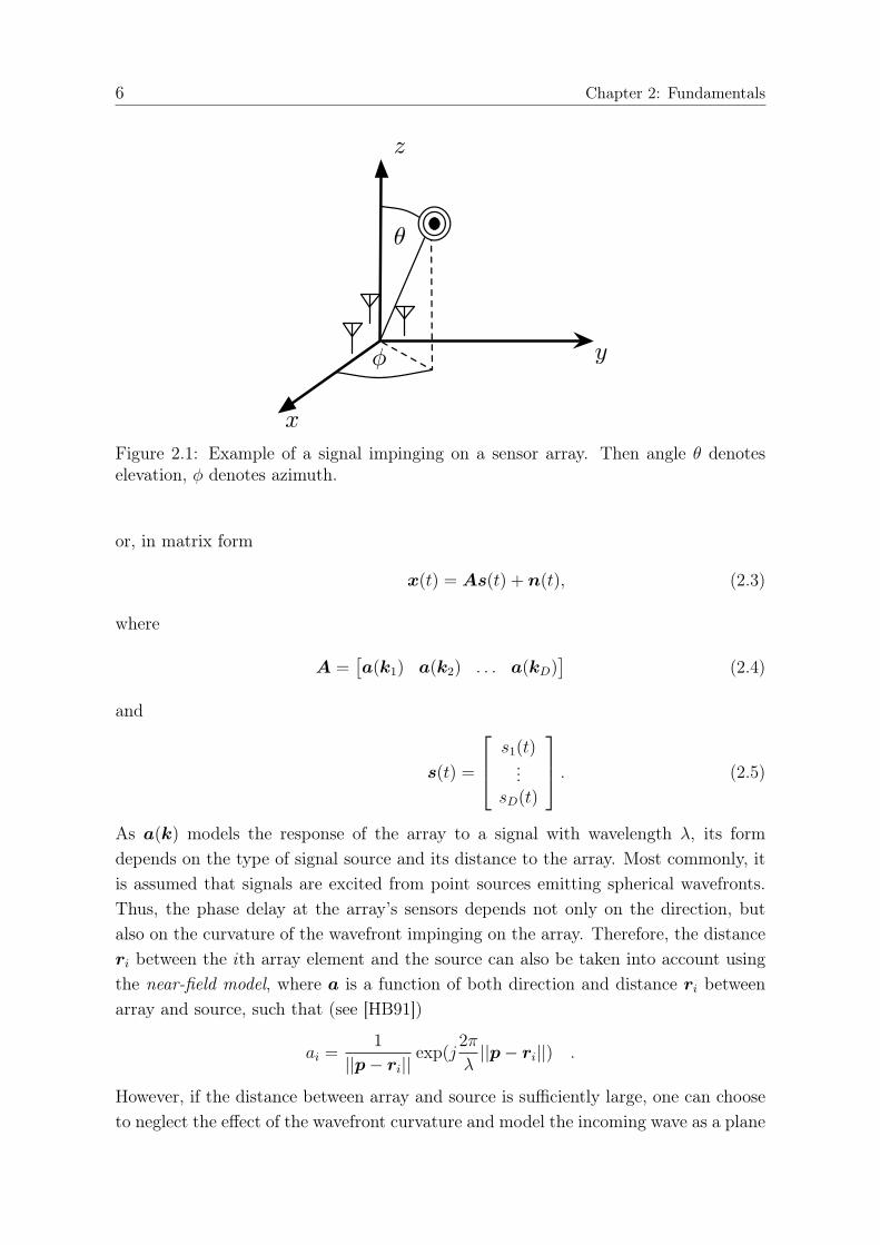
To introduce the standard signal model, we consider a narrow-band signal from un-known direction (θ, φ) and wavelength λ impinging on an array with N elements, withφ being the azimuth and θ the elevation angle (see Fig. 2.1). The position of the ithelement in the array is denoted by position vector pi, i = 1, . . . , N . The output of thearray at time t is denoted by
x(t) = a(k)s(t) + n(t) (2.1)
where
a(k) =
a1(k,p1)...
aN(k,pN)
is the array manifold vector which models the spatial characteristics such as phasedelays and attenuation of the signal impinging on the array’s sensors, s(t) is the complexbaseband signal and n(t) is assumed to be spatially white noise with variance σ2
n.1 IfD > 1 signals impinge on the array, the output will be the superposition of the singlereceived waveforms, e.g.,
x(t) =D∑d
a(kd)sd(t) + n(t), (2.2)
1Since the sensor positions are normally fixed, we drop the dependence of a on the sensor positionsin the notation for most of this work except in Chapter 3.2, where the positions are assumed to benot perfectly known.
6 Chapter 2: Fundamentals
Figure 2.1: Example of a signal impinging on a sensor array. Then angle θ denoteselevation, φ denotes azimuth.
or, in matrix form
x(t) = As(t) + n(t), (2.3)
where
A =[a(k1) a(k2) . . . a(kD)
](2.4)
and
s(t) =
s1(t)...
sD(t)
. (2.5)
As a(k) models the response of the array to a signal with wavelength λ, its formdepends on the type of signal source and its distance to the array. Most commonly, itis assumed that signals are excited from point sources emitting spherical wavefronts.Thus, the phase delay at the array’s sensors depends not only on the direction, butalso on the curvature of the wavefront impinging on the array. Therefore, the distanceri between the ith array element and the source can also be taken into account usingthe near-field model, where a is a function of both direction and distance ri betweenarray and source, such that (see [HB91])
ai =1
||p− ri||exp(j
2π
λ||p− ri||) .
However, if the distance between array and source is sufficiently large, one can chooseto neglect the effect of the wavefront curvature and model the incoming wave as a plane
2.1 Fundamentals of Array Signal Processing 7
wave, resulting in the far-field model. This model is only applicable if the approximationof the wavefront as a plane wave can be justified. The critical distance after which thiscan be safely assumed is decided on by some rules of thumb, e.g., the Fraunhoferdistance which states that
||r|| � 2L2
λ,
with L being the largest dimension of the antenna array. The resulting form for thearray manifold vector is then simply
a(k) =
ejkTp1
...ejk
TpN
, (2.6)
where
k = −2π
λ
sin(θ) cos(φ)sin(θ) sin(φ)
cos(θ)
(2.7)
is the wave vector expressed in Cartesian coordinates. Since ||k|| = k = 2πλ
is the wavenumber and the vector in Eq. (2.7) denotes a vector in unit space, k simply refers toan impinging wave with wavelength λ and points into the direction of its arrival. As itis only the phase differences which contain the information about the direction of thesignals, a(k) can be normalized such that a1 = 1 without loss of information. If thesignals stem not from point sources, but are spatially extended in their dimensions,they can be modeled as the superposition of point sources. Alternatively, one canmodel the signal by a spatial basis function: A point source would correspond to aspatial dirac delta function, but a spatially extended signal, e.g. due to fading or localscattering at the source is modeled by a physically justifiable basis function such asa Gaussian [Tap02,BV98]. Often, the sensor arrays in an application are of a regulargeometry, e.g., a Uniform Linear Array (ULA) or a Uniform Rectangular Array (URA)where the distances between sensor’s position are uniform. This regularity is thenalso present in the array response vector which then shows a Vandermonde structure.This can be exploited for an efficient implementation of the array signal processingmethods. For example, using conventional beamforming as explained below will resultin the possibility to perform DOA estimation using a spatial Fourier transform, forwhich the Vandermonde structure in a ULA or a URA leads to a spatial Fast FourierTransform (FFT). Also the symmetry in other geometries such as Uniform CircularArrays (UCAs) can be exploited by an FFT by transforming the array into a domainwhere the array is then a virtual ULA (see e.g. [DD94a,DD94b,DD94c]).
8 Chapter 2: Fundamentals
2.1.2 Beamforming
The term beamforming denotes a technique where the array elements are weightedsuch that its spatial characteristics can be manipulated. This allows to control thedirectivity of the array in order to spatially filter the received data, i.e. suppressnoise and interference from undesired directions. The two-dimensional spatial powerspectrum P (k) of a signal scenario can be estimated by applying a weighting vectorw(k) to the array data using an estimate RXX of the spatial covariance matrix RXX
of the received data in x(t). By doing so, we obtain the filter output
y(t) = w(k)Hx(t) .
The resulting spatial spectrum estimate is then
P (k) = w(k)HRXXw(k) . (2.8)
While imaging applications demand for a high accuracy of P (k) in the region of interest,the only figure of merit for DOA estimation is the accuracy of the estimator of (θ, φ).In beamforming, the estimator is typically
(θ, φ) = arg max(θ,φ)
P (θ, φ) . (2.9)
A natural choice for RXX is the sample covariance matrix, as it is the maximumlikelihood estimator (MLE) of RXX in white Gaussian noise [VVB88]. Using K datasamples, it is defined as
RXX =1
K
K∑t=1
x(t)x(t)H .
The most intuitive choice for w(k) results in the delay-and-sum beamformer, whichis also called Bartlett beamformer [HJOK85]. Here, the elements of w(k) are simplychosen according to the array manifold vector such that the occurring phase differencesare compensated by delaying all array channels such that their output is coherent again.As the signal from direction kl is recorded with phase shifts in all data channels,choosing
w(kl) =1
Na(kl)
will weigh all channels differently such that a signal impinging with kl is summed upcoherently. Since other signals and the spatial noise impinge from other directions thanthe look direction, this results in a gain in Signal-to-Noise Ratio (SNR) because theyadd up non-coherently, effectively reducing their power in y(t). The resulting powerspectrum estimate is
PBartlett(k) =aH(kl)RXXa(kl)
aH(kl)a(kl).
2.1 Fundamentals of Array Signal Processing 9
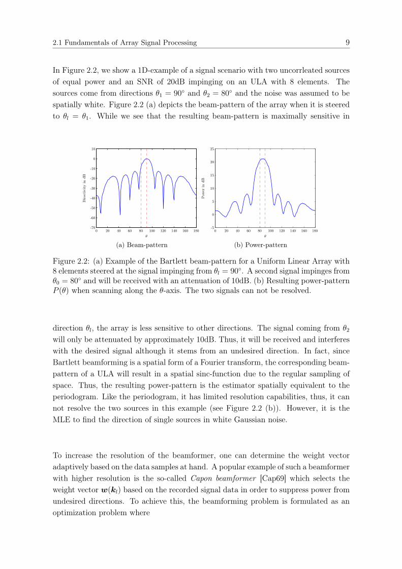
In Figure 2.2, we show a 1D-example of a signal scenario with two uncorrleated sourcesof equal power and an SNR of 20dB impinging on an ULA with 8 elements. Thesources come from directions θ1 = 90◦ and θ2 = 80◦ and the noise was assumed to bespatially white. Figure 2.2 (a) depicts the beam-pattern of the array when it is steeredto θl = θ1. While we see that the resulting beam-pattern is maximally sensitive in
(a) Beam-pattern (b) Power-pattern
Figure 2.2: (a) Example of the Bartlett beam-pattern for a Uniform Linear Array with8 elements steered at the signal impinging from θl = 90◦. A second signal impinges fromθ0 = 80◦ and will be received with an attenuation of 10dB. (b) Resulting power-patternP (θ) when scanning along the θ-axis. The two signals can not be resolved.
direction θl, the array is less sensitive to other directions. The signal coming from θ2
will only be attenuated by approximately 10dB. Thus, it will be received and interfereswith the desired signal although it stems from an undesired direction. In fact, sinceBartlett beamforming is a spatial form of a Fourier transform, the corresponding beam-pattern of a ULA will result in a spatial sinc-function due to the regular sampling ofspace. Thus, the resulting power-pattern is the estimator spatially equivalent to theperiodogram. Like the periodogram, it has limited resolution capabilities, thus, it cannot resolve the two sources in this example (see Figure 2.2 (b)). However, it is theMLE to find the direction of single sources in white Gaussian noise.
To increase the resolution of the beamformer, one can determine the weight vectoradaptively based on the data samples at hand. A popular example of such a beamformerwith higher resolution is the so-called Capon beamformer [Cap69] which selects theweight vector w(kl) based on the recorded signal data in order to suppress power fromundesired directions. To achieve this, the beamforming problem is formulated as anoptimization problem where
10 Chapter 2: Fundamentals
w(kl) = arg minw
(P (w)) (2.10)
subject to w(kl)Ha(kl) = 1 .
The solution of this problem yields
wc(kl) =R−1XXa(kl)
aH(kl)R−1XXa(kl)
(2.11)
and the resulting power spectrum is
PCapon(k) =1
aH(kl)R−1XXa(kl)
. (2.12)
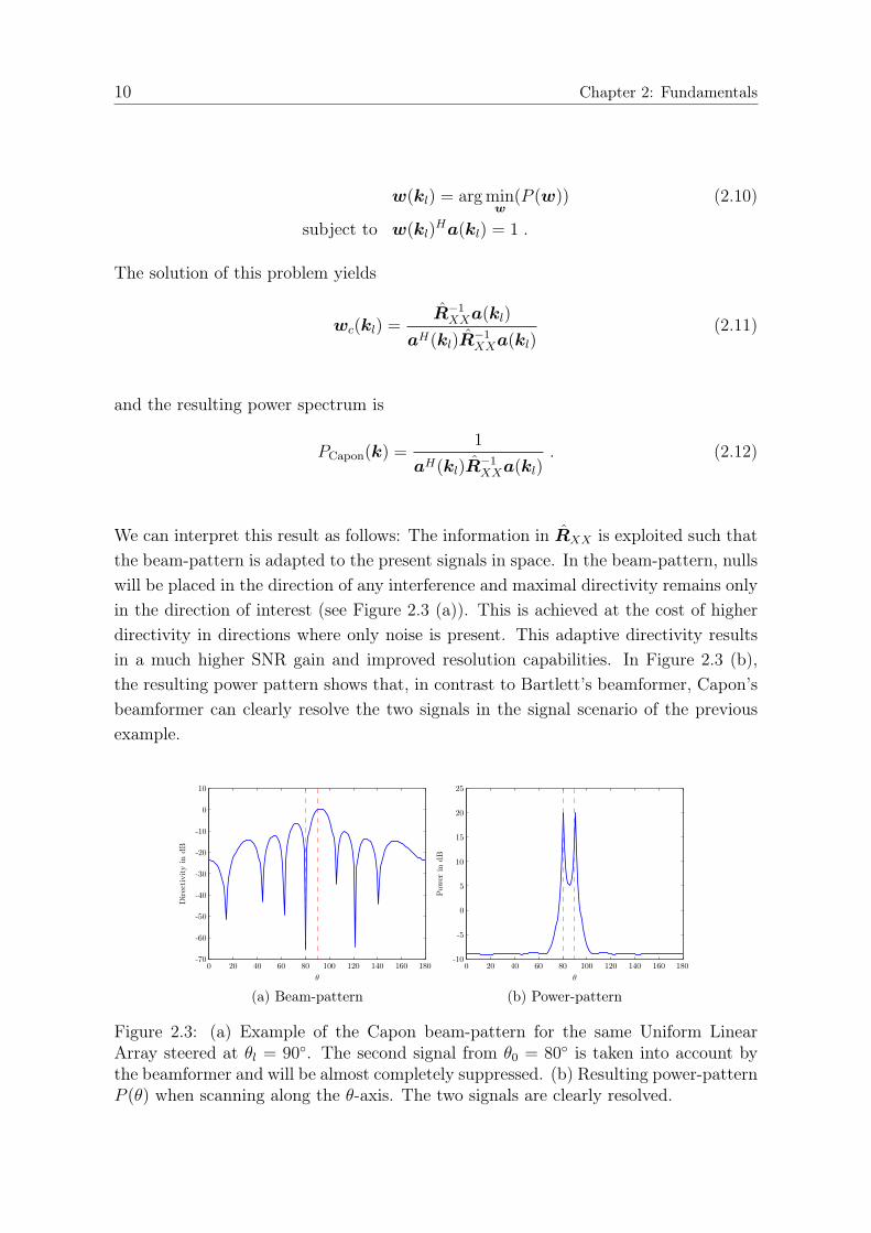
We can interpret this result as follows: The information in RXX is exploited such thatthe beam-pattern is adapted to the present signals in space. In the beam-pattern, nullswill be placed in the direction of any interference and maximal directivity remains onlyin the direction of interest (see Figure 2.3 (a)). This is achieved at the cost of higherdirectivity in directions where only noise is present. This adaptive directivity resultsin a much higher SNR gain and improved resolution capabilities. In Figure 2.3 (b),the resulting power pattern shows that, in contrast to Bartlett’s beamformer, Capon’sbeamformer can clearly resolve the two signals in the signal scenario of the previousexample.
(a) Beam-pattern (b) Power-pattern
Figure 2.3: (a) Example of the Capon beam-pattern for the same Uniform LinearArray steered at θl = 90◦. The second signal from θ0 = 80◦ is taken into account bythe beamformer and will be almost completely suppressed. (b) Resulting power-patternP (θ) when scanning along the θ-axis. The two signals are clearly resolved.
2.1 Fundamentals of Array Signal Processing 11
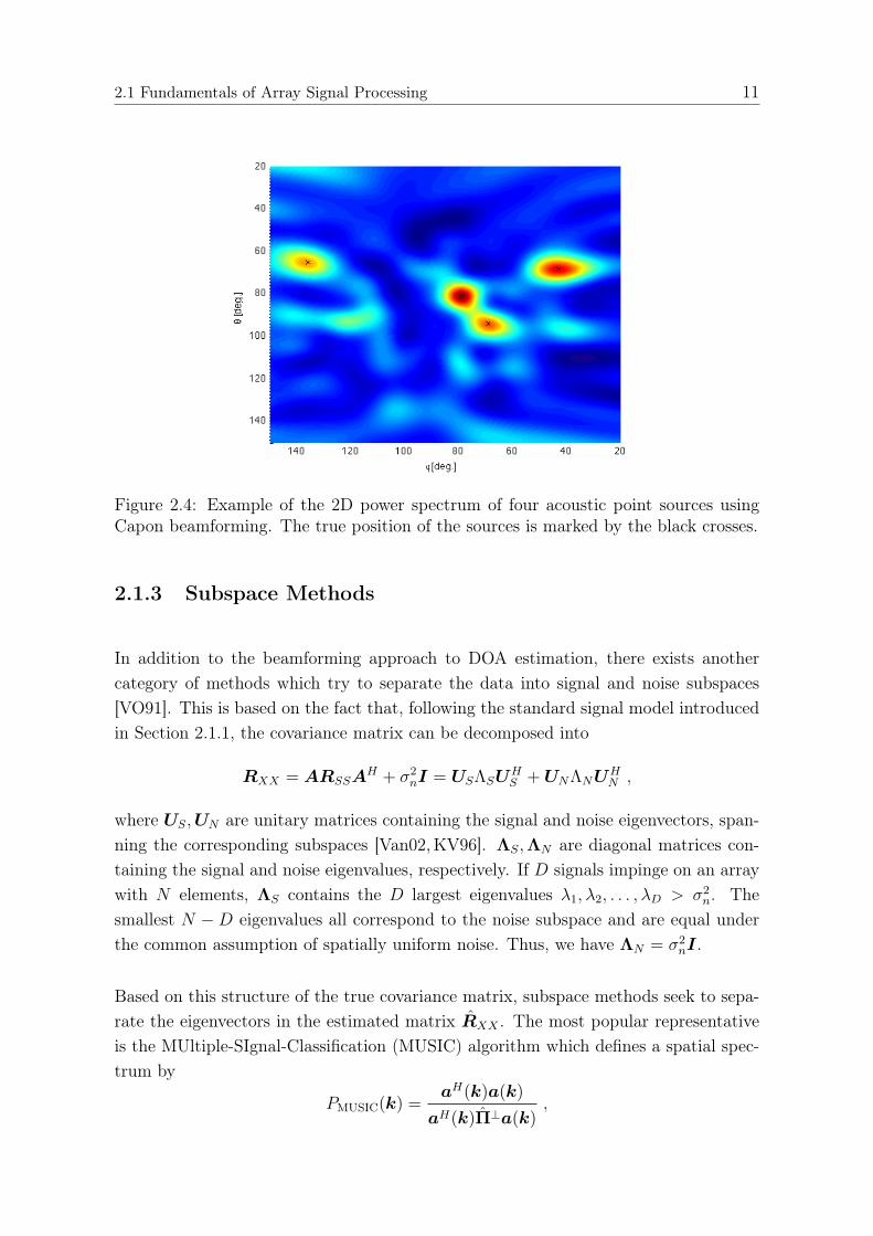
Figure 2.4: Example of the 2D power spectrum of four acoustic point sources usingCapon beamforming. The true position of the sources is marked by the black crosses.
2.1.3 Subspace Methods
In addition to the beamforming approach to DOA estimation, there exists anothercategory of methods which try to separate the data into signal and noise subspaces[VO91]. This is based on the fact that, following the standard signal model introducedin Section 2.1.1, the covariance matrix can be decomposed into
RXX = ARSSAH + σ2
nI = USΛSUHS +UNΛNU
HN ,
where US,UN are unitary matrices containing the signal and noise eigenvectors, span-ning the corresponding subspaces [Van02,KV96]. ΛS,ΛN are diagonal matrices con-taining the signal and noise eigenvalues, respectively. If D signals impinge on an arraywith N elements, ΛS contains the D largest eigenvalues λ1, λ2, . . . , λD > σ2
n. Thesmallest N −D eigenvalues all correspond to the noise subspace and are equal underthe common assumption of spatially uniform noise. Thus, we have ΛN = σ2
nI.
Based on this structure of the true covariance matrix, subspace methods seek to sepa-rate the eigenvectors in the estimated matrix RXX . The most popular representativeis the MUltiple-SIgnal-Classification (MUSIC) algorithm which defines a spatial spec-trum by
PMUSIC(k) =aH(k)a(k)
aH(k)Π⊥a(k),
12 Chapter 2: Fundamentals
where Π⊥ = UNUHN [Sch86]. This is often referred to as a pseudo-spectrum, because
due to the subspace projection it has no physical meaning anymore. It is simplythe result of minimizing the power in the estimated noise subspace by the MUSICalgorithm. Alternatively, one could also change the numerator to aH(k)USU
HS a(k)
and maximize the power in the estimated signal subspace. Since the DOAs of thesignals are found by projections of the data on subspaces, there is no scanning of theenvironment involved and it is not possible to establish direct measures of directivitysuch as a beam-pattern for such methods.
(a) Angular separation of 10◦ (b) Angular separation of 1◦
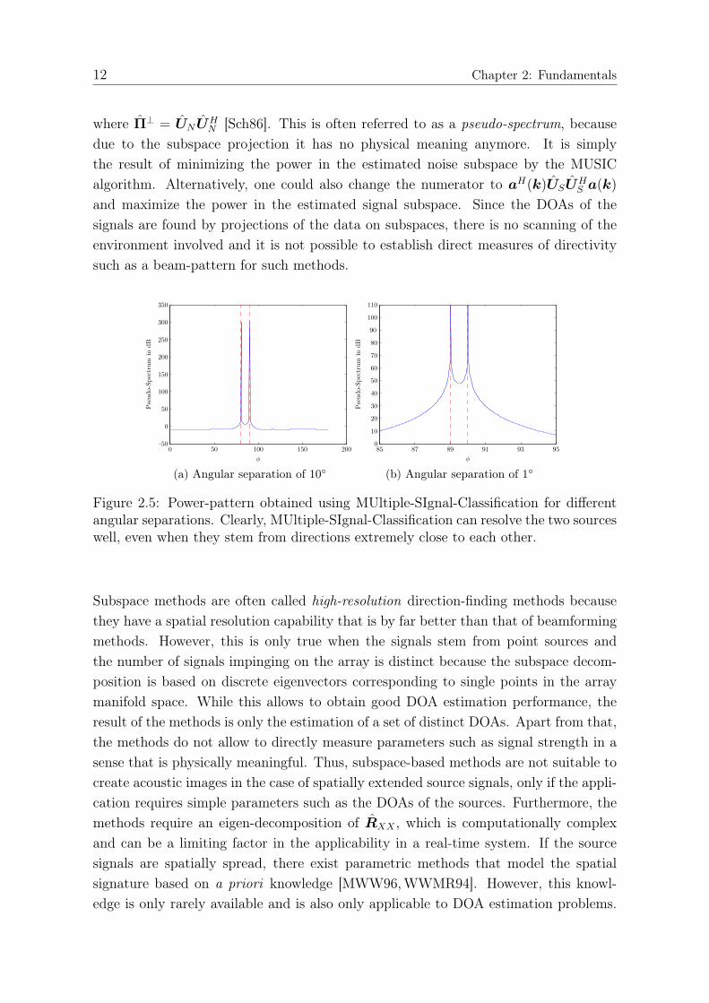
Figure 2.5: Power-pattern obtained using MUltiple-SIgnal-Classification for differentangular separations. Clearly, MUltiple-SIgnal-Classification can resolve the two sourceswell, even when they stem from directions extremely close to each other.
Subspace methods are often called high-resolution direction-finding methods becausethey have a spatial resolution capability that is by far better than that of beamformingmethods. However, this is only true when the signals stem from point sources andthe number of signals impinging on the array is distinct because the subspace decom-position is based on discrete eigenvectors corresponding to single points in the arraymanifold space. While this allows to obtain good DOA estimation performance, theresult of the methods is only the estimation of a set of distinct DOAs. Apart from that,the methods do not allow to directly measure parameters such as signal strength in asense that is physically meaningful. Thus, subspace-based methods are not suitable tocreate acoustic images in the case of spatially extended source signals, only if the appli-cation requires simple parameters such as the DOAs of the sources. Furthermore, themethods require an eigen-decomposition of RXX , which is computationally complexand can be a limiting factor in the applicability in a real-time system. If the sourcesignals are spatially spread, there exist parametric methods that model the spatialsignature based on a priori knowledge [MWW96,WWMR94]. However, this knowl-edge is only rarely available and is also only applicable to DOA estimation problems.
2.1 Fundamentals of Array Signal Processing 13
Thus, when the spatial spread of the sources is not negligible, but unknown, the useof beamforming methods is preferable. Generally, the algorithms require knowledgeabout the number of sources present in the data. This knowledge is usually unavail-able and the number of signals has to be estimated using information criteria suchas the Akaike Information Criterion (AIC) or Minimum Description Length (MDL)(see [SS04,Aka74,WK85,WZ89,WZ88] for an overview of information criteria).
2.1.4 Coherent Sources
While it is generally fruitful to exploit information from the data, the performance ofadaptive methods is degraded when the signal scenarios are complicated. While allmethods suffer from an inaccurate estimation of the covariance matrix due to a smallsample size or low SNR, specific problems can arise when the signals impinging on thearray are correlated or even coherent [SK93, SS98, LVL05,KV96]. While coherent orstrongly correlated signals may generally occur in communications, radar and sonardue to jamming or multi-path propagation, they also occur in acoustic imaging whensimilar objects reflect the signal back to the array. This effect can reduce the resolutioncapabilities of spatial methods or even lead to their failure. For example, when signalsources are correlated, it is harder for Capon’s beamformer to suppress signals fromdirections other than the look direction when they are correlated to a signal fromthat direction. More severely, coherent signals even lead to a rank-deficiency in RXX ,meaning that signal eigenvectors will deviate into the noise subspace and the signalsubspace will be reduced in dimension [KV96]. Thus, adaptive methods, which rely onthe estimated covariance matrix, may fail because they normally assume a full-rankcovariance matrix in the underlying signal model. To overcome these problems, thereexist decorrelation methods that allow to improve the performance in the situationof coherent signals [SWK85,EJS82]. If only two sources are coherent, one can applyforward-backward (FB) averaging to the array. This means that in addition to RXX
a backward matrix is constructed using R∗XX and a selection matrix J with non-zerosonly on the anti-diagonal, which reverses the order of the array’s elements. The twocovariance matrices are averaged such that
RFB =1
2(RXX + JR∗XXJ) .
which is then used in lieu of R. This effectively decorrelates the two coherent sources. IfD > 2 sources are coherent, one can use spatial smoothing which generalizes the idea ofFB averaging by using at least D sub-arrays and the corresponding covariance matricesRd, d = 1, . . . , D [SK85]. If the sub-arrays are identical in shape, the corresponding
14 Chapter 2: Fundamentals
covariance matrices are assumed to be identical up to a scaling factor which dependsonly on the geometric distance between the sub-arrays. Thus, averaging the smallercovariance matrices leads to a smoothed covariance matrix
RD =1
D
D∑d=1
Rd
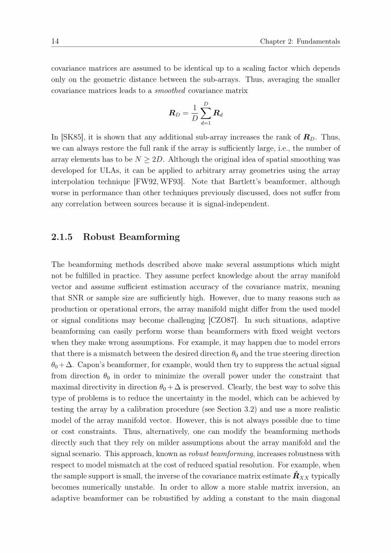
In [SK85], it is shown that any additional sub-array increases the rank of RD. Thus,we can always restore the full rank if the array is sufficiently large, i.e., the number ofarray elements has to be N ≥ 2D. Although the original idea of spatial smoothing wasdeveloped for ULAs, it can be applied to arbitrary array geometries using the arrayinterpolation technique [FW92,WF93]. Note that Bartlett’s beamformer, althoughworse in performance than other techniques previously discussed, does not suffer fromany correlation between sources because it is signal-independent.
2.1.5 Robust Beamforming
The beamforming methods described above make several assumptions which mightnot be fulfilled in practice. They assume perfect knowledge about the array manifoldvector and assume sufficient estimation accuracy of the covariance matrix, meaningthat SNR or sample size are sufficiently high. However, due to many reasons such asproduction or operational errors, the array manifold might differ from the used modelor signal conditions may become challenging [CZO87]. In such situations, adaptivebeamforming can easily perform worse than beamformers with fixed weight vectorswhen they make wrong assumptions. For example, it may happen due to model errorsthat there is a mismatch between the desired direction θ0 and the true steering directionθ0 +∆. Capon’s beamformer, for example, would then try to suppress the actual signalfrom direction θ0 in order to minimize the overall power under the constraint thatmaximal directivity in direction θ0 + ∆ is preserved. Clearly, the best way to solve thistype of problems is to reduce the uncertainty in the model, which can be achieved bytesting the array by a calibration procedure (see Section 3.2) and use a more realisticmodel of the array manifold vector. However, this is not always possible due to timeor cost constraints. Thus, alternatively, one can modify the beamforming methodsdirectly such that they rely on milder assumptions about the array manifold and thesignal scenario. This approach, known as robust beamforming, increases robustness withrespect to model mismatch at the cost of reduced spatial resolution. For example, whenthe sample support is small, the inverse of the covariance matrix estimate RXX typicallybecomes numerically unstable. In order to allow a more stable matrix inversion, anadaptive beamformer can be robustified by adding a constant to the main diagonal

2.2 Fundamentals of Classification 15
of RXX . This is equivalent to adding artificial noise and allows to stabilize the maindiagonal of RXX [LSW03]. This technique, which is called diagonal loading, is a generalmeans of robustification of adaptive beamforming techniques. The resulting covariancematrix RXX can be described as
RXX = RXX + σ2DLI . (2.13)
The choice of the loading value σ2DL can only be determined optimally if a measure of
uncertainty on the existing errors is available, otherwise, it has to be set empirically (e.g.[LSW03]). Often, one finds that σ2
DL
σ2n
= 10 is used, where σ2n is an estimate of the average
power on the main diagonal of RXX [Van02]. The concept of diagonal loading providesan easy way to balance the degree of adaptivity of a beamformer. For example, if theartificial noise power is increased, the main diagonal of RXX becomes more dominantand the beamformer performs more like Bartlett’s beamformer. In [Ric07,Ric10], thecorrelation between the two beamformers is studied and it is shown how the correctdegree of adaptivity can improve the spatial resolution for DOA estimation problems.
2.2 Fundamentals of Classification
Classification is the task to assign a class label Cn, where n = 1, . . . , N , to an inputvector f in order to classify it as belonging to one of N discrete classes. Clearly, thedefinition of classes is problem-dependent and while it is most commonly assumed thatthe data classes are disjoint, this assumption may not hold for specific problems, e.g.,when a person walks, it will resemble a standing person during certain parts of themovement (see Section 5.5). The input vector consists of features that are extracted inprior stages, they describe specific characteristics from data derived from a lower level,e.g., an image that is obtained from raw sensor data or specific descriptors of that image.A classifier divides the feature space into decision regions and the different classificationmethods differ in the way they formulate and obtain the decision boundaries betweenthe classes. In the context of classification, the array signal processing pursued to obtain3D images can be interpreted simply as a way to create data from which features areextracted. In this section, we introduce some of the approaches to machine learningthat we use for the classification of acoustic imaging data. However, we do restrict thediscussion here to the applied classifiers and do not cover other powerful approaches,e.g., neural networks or Markov random fields. Moreover, we present the theory in thecontext of two-class problems for simplicity and because we do not apply the methodsto multi-class problems in this thesis. For a more complete and in-depth introductionto the general field of classification, we refer the reader to [Bis07,DHS01].
16 Chapter 2: Fundamentals
2.2.1 Discriminant Functions
A discriminant function takes a D-dimensional input vector f and maps it directly toa class label Cn by some transformation of the data. In its simplest form, the functionis linear such that
y(f) = wTf + w0 , (2.14)
where w is a weighting vector and w0 is a threshold sometimes called bias. If y(f) ≥ 0,the input is assigned to C1 and to C2 otherwise. If K > 2, one would construct Kdiscriminant functions and obtain decisions by linearly combining them. Therefore,the decision boundary is defined by y(f) = 0 and is a hyperplane with dimension(D − 1).
2.2.1.1 Fisher’s Linear Discriminant
In its most simple form, the input f is weighted linearly as shown above. The taskof obtaining a good classifier can then be interpreted as the task to geometrically findthe projection direction, represented by w, that separates the data well into the twoclasses. Fisher’s Linear Discriminant defines a criterion for this class-separability bytaking both the distance between classes as well as the distribution within the classesinto account. The inter-class distance, also called between-class scatter, is measuredby
m1 −m2 ,
where mi is the mean vector of the ith class. We use it in its quadratic form, denotedby
ΣB = (m1 −m2)(m1 −m2)T (2.15)
as the inter-class scatter matrix. To measure the total intra-class distance of the data,we can simply use the sum of the covariance matrices inside the classes, each given by
Σi =∑f∈Ci
(f −mi)(f −mi)T . (2.16)
This results in the intra-class scatter matrix
ΣW = Σ1 + Σ2 . (2.17)
When the data is weighted by w, these distances can be expressed as wTΣBw andwTΣWw, respectively. To find the weighting vector that maximizes the class separa-bility, the ratio of inter-and intra-class distances
J(w) =wTΣBw
wTΣWw(2.18)
2.2 Fundamentals of Classification 17
is maximized with respect to w. Assuming ΣW to be non-singular, the optimal w isthen
wopt = Σ−1W (m1 −m2) .
When this approach is used for classification, it is denoted Linear Discriminant Analysis(LDA). It implicitly assumes that the classes share common covariance matrix, whichcan be unrealistic. However, the input has limited sample size and mostly no knowl-edge about the class distribution or its parameters mi,Σi is available. Thus, theseparameters have to be estimated using training data.
2.2.1.2 Generalized Linear Discriminants
The principle of LDA can be generalized to a weighting function that consists of alinear combination of more complex function, e.g. by
y(f) =d∑i=0
aig(f) , (2.19)
where g(·) is some arbitrary function of the input. For example, a Quadratic Dis-criminant Analysis (QDA) uses a quadratic function of the input vector f and findsweightings based on that. As a result, the decision boundaries in the feature space willalso be of quadratic form. Clearly, this allows better class separation in cases wherethe classes are not well separated. At the same time, a more complex function g(·)can be the result of more general assumptions on the data, e.g., that the classes havedifferent covariance matrices.
2.2.2 Support Vector Machines
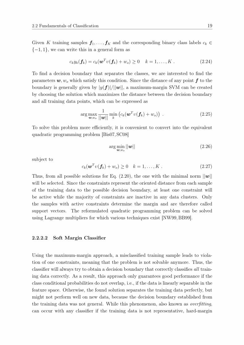
A powerful method to build a classifier is to form the decision boundaries not fromfunctions of a specific form, but from the data directly. In contrast to parametricmodels which find a weighting vector w and then project any test data, the idea ofSupport Vector Machines (SVMs) is to determine the decision boundary based onsingle input vectors from the training data, the support vectors, which are close tothe boundary. The boundary is chosen such that the maximum of data points in thetraining data is lying on the correct side of the boundary. It can be shown that findingthe parameters of the boundary is always a convex optimization problem. However,training of a SVM can be computationally complex and in practice, some parametershave to be chosen manually which can highly influence the performance. We will show
18 Chapter 2: Fundamentals
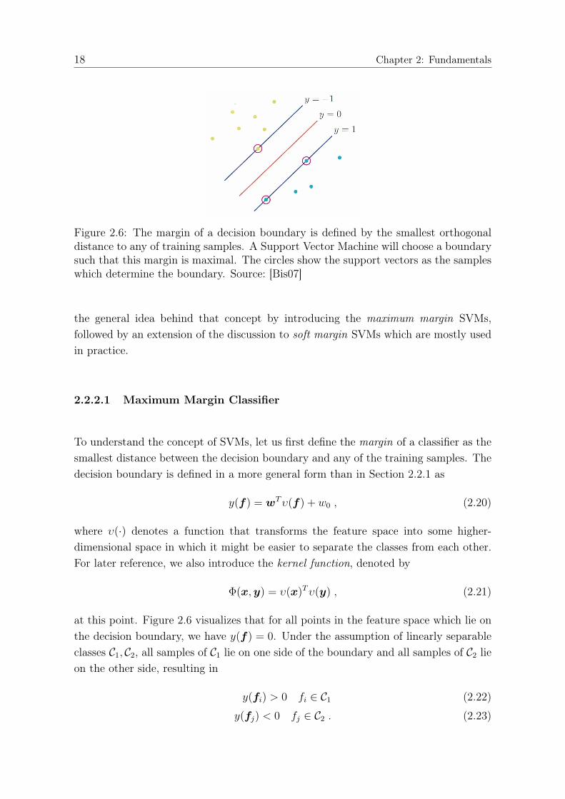
Figure 2.6: The margin of a decision boundary is defined by the smallest orthogonaldistance to any of training samples. A Support Vector Machine will choose a boundarysuch that this margin is maximal. The circles show the support vectors as the sampleswhich determine the boundary. Source: [Bis07]
the general idea behind that concept by introducing the maximum margin SVMs,followed by an extension of the discussion to soft margin SVMs which are mostly usedin practice.
2.2.2.1 Maximum Margin Classifier
To understand the concept of SVMs, let us first define the margin of a classifier as thesmallest distance between the decision boundary and any of the training samples. Thedecision boundary is defined in a more general form than in Section 2.2.1 as
y(f) = wTυ(f) + w0 , (2.20)
where υ(·) denotes a function that transforms the feature space into some higher-dimensional space in which it might be easier to separate the classes from each other.For later reference, we also introduce the kernel function, denoted by
Φ(x,y) = υ(x)Tυ(y) , (2.21)
at this point. Figure 2.6 visualizes that for all points in the feature space which lie onthe decision boundary, we have y(f) = 0. Under the assumption of linearly separableclasses C1, C2, all samples of C1 lie on one side of the boundary and all samples of C2 lieon the other side, resulting in
y(fi) > 0 fi ∈ C1 (2.22)
y(fj) < 0 fj ∈ C2 . (2.23)
2.2 Fundamentals of Classification 19
Given K training samples f1, . . . ,fK and the corresponding binary class labels ck ∈{−1, 1}, we can write this in a general form as
ckyk(fk) = ck(wTυ(fk) + wo) ≥ 0 k = 1, . . . , K . (2.24)
To find a decision boundary that separates the classes, we are interested to find theparameters w, wo which satisfy this condition. Since the distance of any point f to theboundary is generally given by |y(f)|/||w||, a maximum-margin SVM can be createdby choosing the solution which maximizes the distance between the decision boundaryand all training data points, which can be expressed as
arg maxw,wo
1
||w||mink
(ck(w
Tυ(fk) + wo)). (2.25)
To solve this problem more efficiently, it is convenient to convert into the equivalentquadratic programming problem [Bis07,SC08]
arg minw,wo||w|| (2.26)
subject tock(w
Tυ(fk) + wo) ≥ 0 k = 1, . . . , K . (2.27)
Thus, from all possible solutions for Eq. (2.20), the one with the minimal norm ||w||will be selected. Since the constraints represent the oriented distance from each sampleof the training data to the possible decision boundary, at least one constraint willbe active while the majority of constraints are inactive in any data clusters. Onlythe samples with active constraints determine the margin and are therefore calledsupport vectors. The reformulated quadratic programming problem can be solvedusing Lagrange multipliers for which various techniques exist [NW99,BB99].
2.2.2.2 Soft Margin Classifier
Using the maximum-margin approach, a misclassified training sample leads to viola-tion of one constraints, meaning that the problem is not solvable anymore. Thus, theclassifier will always try to obtain a decision boundary that correctly classifies all train-ing data correctly. As a result, this approach only guarantees good performance if theclass conditional probabilities do not overlap, i.e., if the data is linearly separable in thefeature space. Otherwise, the found solution separates the training data perfectly, butmight not perform well on new data, because the decision boundary established fromthe training data was not general. While this phenomenon, also known as overfitting,can occur with any classifier if the training data is not representative, hard-margin
20 Chapter 2: Fundamentals
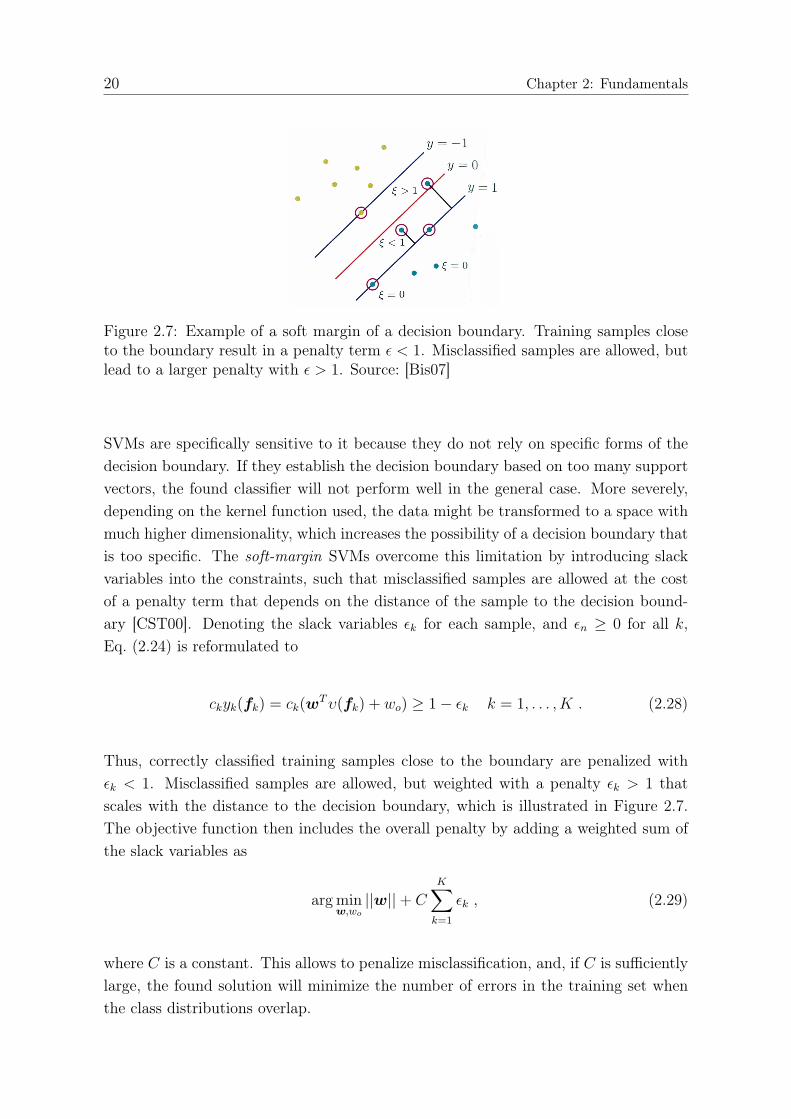
Figure 2.7: Example of a soft margin of a decision boundary. Training samples closeto the boundary result in a penalty term ε < 1. Misclassified samples are allowed, butlead to a larger penalty with ε > 1. Source: [Bis07]
SVMs are specifically sensitive to it because they do not rely on specific forms of thedecision boundary. If they establish the decision boundary based on too many supportvectors, the found classifier will not perform well in the general case. More severely,depending on the kernel function used, the data might be transformed to a space withmuch higher dimensionality, which increases the possibility of a decision boundary thatis too specific. The soft-margin SVMs overcome this limitation by introducing slackvariables into the constraints, such that misclassified samples are allowed at the costof a penalty term that depends on the distance of the sample to the decision bound-ary [CST00]. Denoting the slack variables εk for each sample, and εn ≥ 0 for all k,Eq. (2.24) is reformulated to
ckyk(fk) = ck(wTυ(fk) + wo) ≥ 1− εk k = 1, . . . , K . (2.28)
Thus, correctly classified training samples close to the boundary are penalized withεk < 1. Misclassified samples are allowed, but weighted with a penalty εk > 1 thatscales with the distance to the decision boundary, which is illustrated in Figure 2.7.The objective function then includes the overall penalty by adding a weighted sum ofthe slack variables as
arg minw,wo||w||+ C
K∑k=1
εk , (2.29)
where C is a constant. This allows to penalize misclassification, and, if C is sufficientlylarge, the found solution will minimize the number of errors in the training set whenthe class distributions overlap.

2.2 Fundamentals of Classification 21
2.2.2.3 Choice of the Kernel Function
While the choice of the kernel function directly affects the performance of the classifier,unfortunately there are no theoretical guidelines which help to choose which kernelfunction is appropriate for a given problem. Thus, the choice of a kernel is made basedon experience and often data analysis. Popular kernels include
• the linear kernel Φ(x,y) = xT · y,
• radial basis functions, e.g., Gaussian functionals Φ(x,y) = exp ||x−y||2σ
, with σ
being determined problem-specific by validation procedures,
• and polynomial kernels, e.g. Φ(x,y) = (x · y)d with polynomial order d.
Generally, the more complex the kernel function is, the higher the dimensionality ofthe transformation domain. SVMs solve the classification problem by linear separationof the data in this higher-dimensional space. However, the high dimensionality canalso be problematic, especially if the available training data is limited. In fact, solvingthe problem can become infeasible because the data might be transformed such thatit does not form any reasonable clusters in the transformation space, which makes itimpossible to recognize patterns and separate them.

22
Chapter 3
Design of Acoustic Imaging Systems
In this chapter, we present general design principles for acoustic imaging systems forthe applications of interest. After some basic definitions and an overview of the signalprocessing chain, we present some useful assumptions about the transmission mediumand the signals, as well as some basic characteristics of an acoustic imaging systemwhich operates in air. After we show system-specific properties of the prototypes usedin this thesis, we also show several real-data examples. Additionally, we present cali-bration techniques which are needed as a first step after the production of an acousticarray in order to compensate for inevitable production errors and tolerances. Aftera short review of some general techniques, we present a parametric approach whichis specifically suited for acoustic arrays and how this approach can be combined withtraditional calibration methods.
3.1 Design Principles for Acoustic Imaging Systems
The term acoustic imaging denotes techniques which use acoustic signals in order tocreate images of an object or a scene of interest. In general, an acoustic signal is sent outand the reflections are recorded and processed in order to form an image, although therealso exist passive approaches that strive to simply visualize the originating location ofsounds. In this thesis, we focus on the use of acoustic arrays which allow to process therecorded reflections in order to estimate the spatial location and shape of reflectors (seealso [Ste00,MT00,MT94,PH96]). In the following, we will introduce the assumptionswe make with respect to signal model and propagation, followed by a description of thegeneral steps needed to create a three-dimensional, acoustic image from the recordedreflection data. We will then briefly describe the acoustic imaging system that hasbeen developed and used throughout this work.
3.1.1 Data Processing
To generate 3D images of a scene in air, the main limitation one has to deal with isthe slow speed of propagation. In contrast to other typical imaging applications, wetherefore do not perform beamforming to transmit the signal. A better strategy is to
3.1 Design Principles for Acoustic Imaging Systems 23
Range Gating Segmentation
Beamforming
Beamforming
Beamforming
Demodulation
array
3D Image Formation
transmitter
object in scene
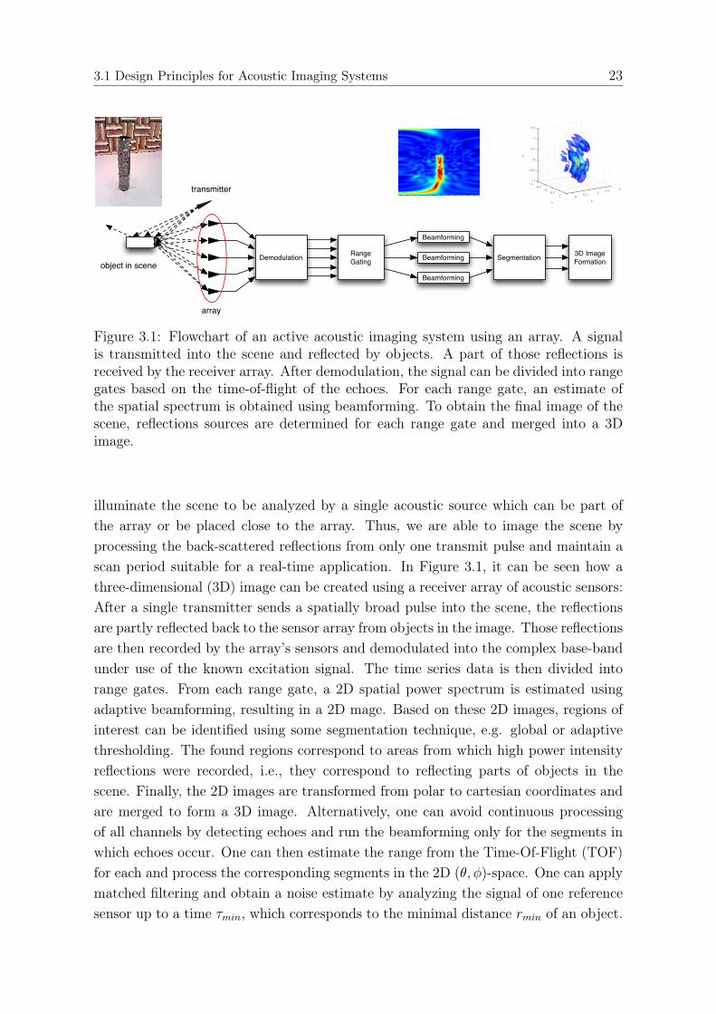
Figure 3.1: Flowchart of an active acoustic imaging system using an array. A signalis transmitted into the scene and reflected by objects. A part of those reflections isreceived by the receiver array. After demodulation, the signal can be divided into rangegates based on the time-of-flight of the echoes. For each range gate, an estimate ofthe spatial spectrum is obtained using beamforming. To obtain the final image of thescene, reflections sources are determined for each range gate and merged into a 3Dimage.
illuminate the scene to be analyzed by a single acoustic source which can be part ofthe array or be placed close to the array. Thus, we are able to image the scene byprocessing the back-scattered reflections from only one transmit pulse and maintain ascan period suitable for a real-time application. In Figure 3.1, it can be seen how athree-dimensional (3D) image can be created using a receiver array of acoustic sensors:After a single transmitter sends a spatially broad pulse into the scene, the reflectionsare partly reflected back to the sensor array from objects in the image. Those reflectionsare then recorded by the array’s sensors and demodulated into the complex base-bandunder use of the known excitation signal. The time series data is then divided intorange gates. From each range gate, a 2D spatial power spectrum is estimated usingadaptive beamforming, resulting in a 2D mage. Based on these 2D images, regions ofinterest can be identified using some segmentation technique, e.g. global or adaptivethresholding. The found regions correspond to areas from which high power intensityreflections were recorded, i.e., they correspond to reflecting parts of objects in thescene. Finally, the 2D images are transformed from polar to cartesian coordinates andare merged to form a 3D image. Alternatively, one can avoid continuous processingof all channels by detecting echoes and run the beamforming only for the segments inwhich echoes occur. One can then estimate the range from the Time-Of-Flight (TOF)for each and process the corresponding segments in the 2D (θ, φ)-space. One can applymatched filtering and obtain a noise estimate by analyzing the signal of one referencesensor up to a time τmin, which corresponds to the minimal distance rmin of an object.
24 Chapter 3: Design of Acoustic Imaging Systems
Since no echoes are assumed to be present in this interval, an estimate σ2n of the noise
floor is calculated. Note that since the noise is assumed to be Additive White GaussianNoise (AWGN), it is sufficient to set rmin to a small value (e.g. rmin = 20 cm).
The estimated noise floor σ2n is then used to determine a threshold to detect echo seg-
ments, where echoes have to occur with a minimal duration of 1 ms. These segmentsare then processed individually by the beamforming algorithm, assuming a range cal-culated from the start of the echo segment, resulting in a dynamic focusing system.Note that the translation of the TOF into range assumes a direct path echo. Addition-ally, due to the possible overlap of different reflections, the length of the echo segmentsmight vary. In that case, the later echo is assigned the same τ as the first one, possiblyintroducing a small range error for some parts of the analyzed scene.
Many of the existing adaptive approaches in array signal processing have been devel-oped for far-field conditions and a finite number of point sources. The imaging systemmust also operate on objects that are close and have a non-negligible spatial spread,such that these algorithms can not always be applied in this problem. We thereforerestrict the system to using beamforming algorithms which do not rely on the assump-tion of point-sources, such as the Capon beamformer (see Section 2.1.2). To obtain animage from a processed echo segment, we scan the environment on a hemisphere witha fine, 2D grid in the θ, φ-space and calculate the received power from each point ina specific range gate. To construct the 3D images, we generally need to decide whichareas of the 2D images contain reflections. Generally, this involves searching for localpeaks at different ranges and deciding based on some segmentation criterion how largethe areas should be and whether the overall peak region is large enough to be consid-ered significant and likely to be related to an object. While the images are obtainedusing beamforming which inevitable has a finite resolution, also the reflections them-selves result in areas of monotonically decreasing power intensity. Thus, compared totraditional image processing problems derived for optical images, the regions of inter-est in the images can be found using relatively low-complexity segmentation methodsbased on adaptive thresholding and similar concepts . In this work we have used theEM algorithm for segmentation which is described in more detail in Section 5.2.
3.1.2 Assumptions and Basic Characteristics
In the following, we make some assumptions about the signal excitation and the phys-ical conditions which are reasonable for acoustic imaging systems and the applicationsof interest:

3.1 Design Principles for Acoustic Imaging Systems 25
1. The scene is illuminated by a narrow-band acoustic signal with center-frequencyfc and wavelength λ, emitted from a single acoustic sensor at a fixed position.
2. Echoes are recorded by an N -element dense array of isotropic acoustic sensorswith uniform noise σn at each element.
3. The array operates in air, i.e. signals propagate in a homogeneous linear mediumwith constant propagation speed (as opposed to human tissue or water) [Boh88].
4. Objects closer than 1m are processed using a near-field signal model, such that thepropagation of the sound echoes can be modeled using Fresnel’s approximation.This follows directly from the wavelength of an acoustic signal in a range of40− 60kHz as well as the array aperture suitable for the application in a robot.
5. Additionally, the objects are assumed to have a solid surface, resulting in largeacoustic impedance differences between air and the materials. This results inhard echoes from the objects. Almost no signal energy is lost due to diffusioninto the object, i.e. the signal does not penetrate the object’s surface.
6. Further, without loss of generality, we assume that the center of the array lies inthe origin of the coordinate system.
When sound is reflected from massive, solid objects, there are three sources of reflectedechoes that are visible to the array: As is illustrated in Figure 3.2, there is a directreflection that occurs from power reflected orthogonally from a planar surface of theobject in a specular way. Additionally, there can be ground reflections where the signalis reflected from the object to ground and vice versa. Clearly, the time-of-flight ofsuch a reflection is longer due to the indirect path it takes. Moreover, such echoes willimpinge on the array from a lower angle and, thus, appear to stem from a reflectionbelow ground. However, to correct this, we simply have to change the sign of the heightcoordinate of those reflections. Clearly, this type of reflection does only occur whenthe object has reflecting areas close to the ground. Most importantly, all solid objectsreflect sounds from their edges, where power is reflected as a superposition of sphericalwaves. In Figure 3.3 (b), we give a real data example where those three distinct regionsare clearly visible. If the object surface is not smooth, the reflection process becomesmore complicated. The echoes return not only from the three sources discussed above.Additionally, the sound wave will be reflected from many parts of the surface whichare orthogonal to the direct path between the array and the surface. This leads toreflections which are spatially more diffuse (see Figure 3.3 (c)). According to acoustictheory, this can be modeled as the superposition of reflections from point sources whichform the surface of the reflecting areas. This effect enables us to obtain information
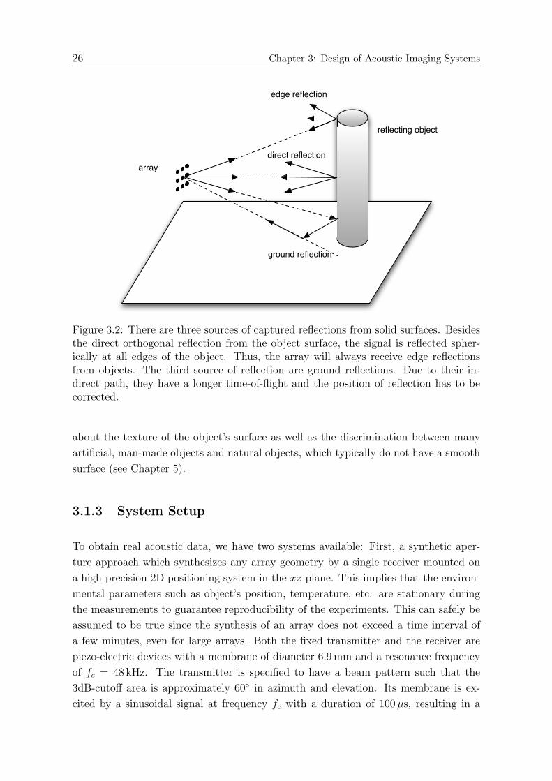
26 Chapter 3: Design of Acoustic Imaging Systems
array
reflecting object
ground reflection
edge reflection
direct reflection
Figure 3.2: There are three sources of captured reflections from solid surfaces. Besidesthe direct orthogonal reflection from the object surface, the signal is reflected spher-ically at all edges of the object. Thus, the array will always receive edge reflectionsfrom objects. The third source of reflection are ground reflections. Due to their in-direct path, they have a longer time-of-flight and the position of reflection has to becorrected.
about the texture of the object’s surface as well as the discrimination between manyartificial, man-made objects and natural objects, which typically do not have a smoothsurface (see Chapter 5).
3.1.3 System Setup
To obtain real acoustic data, we have two systems available: First, a synthetic aper-ture approach which synthesizes any array geometry by a single receiver mounted ona high-precision 2D positioning system in the xz-plane. This implies that the environ-mental parameters such as object’s position, temperature, etc. are stationary duringthe measurements to guarantee reproducibility of the experiments. This can safely beassumed to be true since the synthesis of an array does not exceed a time interval ofa few minutes, even for large arrays. Both the fixed transmitter and the receiver arepiezo-electric devices with a membrane of diameter 6.9 mm and a resonance frequencyof fc = 48 kHz. The transmitter is specified to have a beam pattern such that the3dB-cutoff area is approximately 60◦ in azimuth and elevation. Its membrane is ex-cited by a sinusoidal signal at frequency fc with a duration of 100µs, resulting in a
3.1 Design Principles for Acoustic Imaging Systems 27
narrow-band excitation signal of that frequency and a duration of 1 ms. The receivedanalog signals at the array channels are band-limited before they are sampled at a rateof fs = 200 kHz. The data is then demodulated to obtain the complex base-band sig-nals. The described system is mainly useful for the validation of simulation results inthe array geometry design. In addition to this synthetic aperture system, several arraygeometries were produced by our industry partner, both uniform dense arrays as wellas nonuniform sparse arrays. They allow to capture a scene using a single excitationsignal with a frame rate that is limited only by propagation time and hardware. Forexample, due to the propagation time necessary to record reflections from objects 10maway, the frame rate of a narrow-band system has an upper bound of
fpsmax =1
210mc
=343
20s≈ 17
1
s.
While this would be sufficient for real-time scene analysis, it requires fast hardwarewhich can be a limiting factor in the design of imaging systems for cost-sensitive ap-plications, e.g., for domestic robots.
3.1.4 Real Data Examples
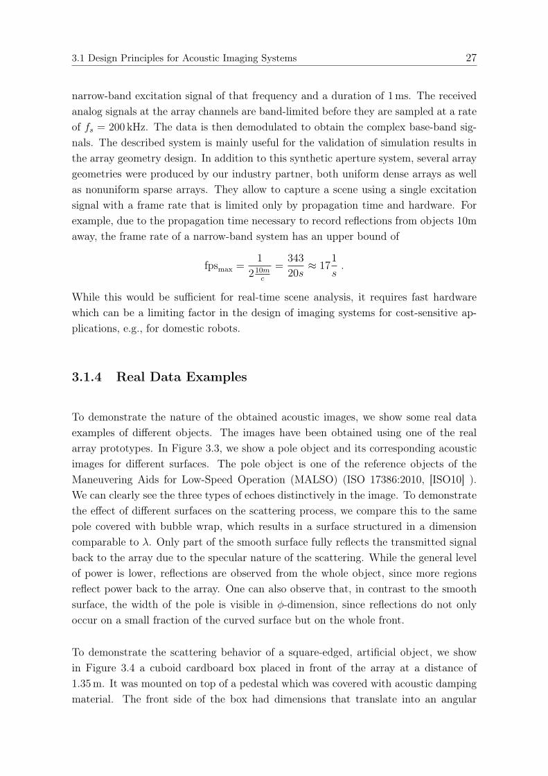
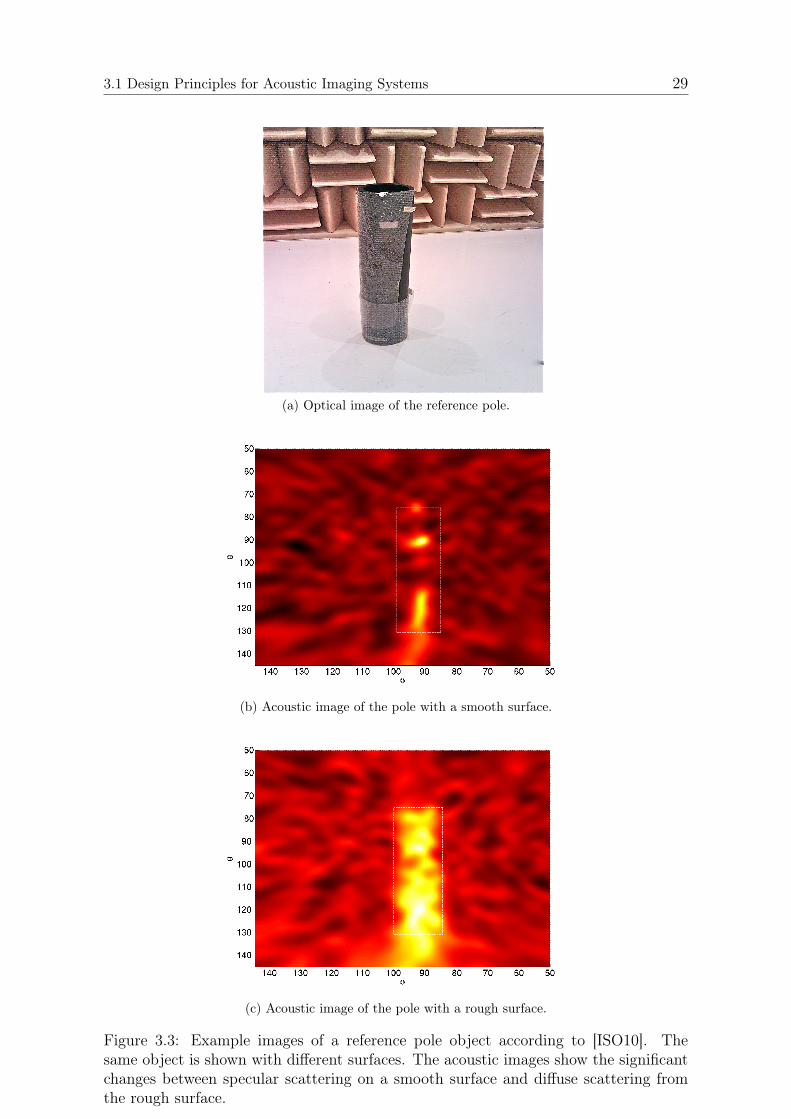
To demonstrate the nature of the obtained acoustic images, we show some real dataexamples of different objects. The images have been obtained using one of the realarray prototypes. In Figure 3.3, we show a pole object and its corresponding acousticimages for different surfaces. The pole object is one of the reference objects of theManeuvering Aids for Low-Speed Operation (MALSO) (ISO 17386:2010, [ISO10] ).We can clearly see the three types of echoes distinctively in the image. To demonstratethe effect of different surfaces on the scattering process, we compare this to the samepole covered with bubble wrap, which results in a surface structured in a dimensioncomparable to λ. Only part of the smooth surface fully reflects the transmitted signalback to the array due to the specular nature of the scattering. While the general levelof power is lower, reflections are observed from the whole object, since more regionsreflect power back to the array. One can also observe that, in contrast to the smoothsurface, the width of the pole is visible in φ-dimension, since reflections do not onlyoccur on a small fraction of the curved surface but on the whole front.
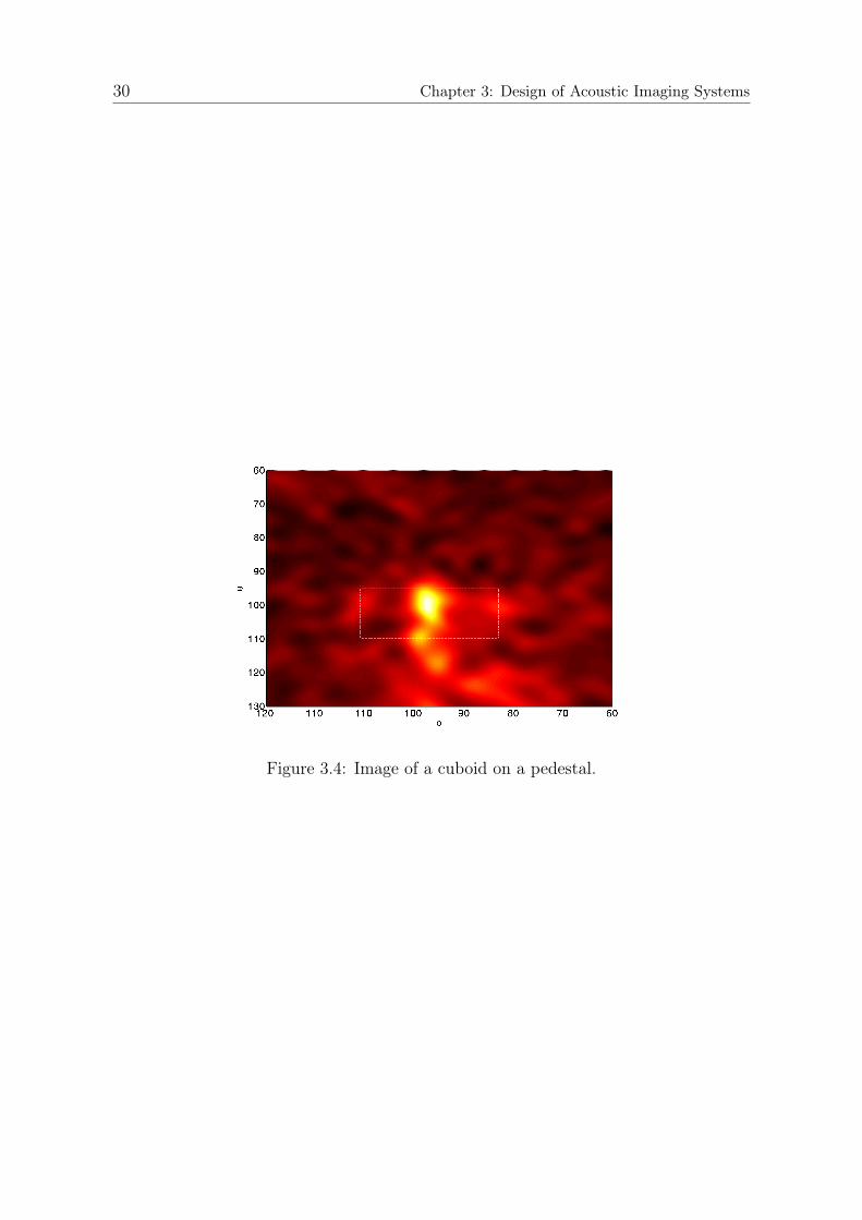
To demonstrate the scattering behavior of a square-edged, artificial object, we showin Figure 3.4 a cuboid cardboard box placed in front of the array at a distance of1.35 m. It was mounted on top of a pedestal which was covered with acoustic dampingmaterial. The front side of the box had dimensions that translate into an angular

28 Chapter 3: Design of Acoustic Imaging Systems
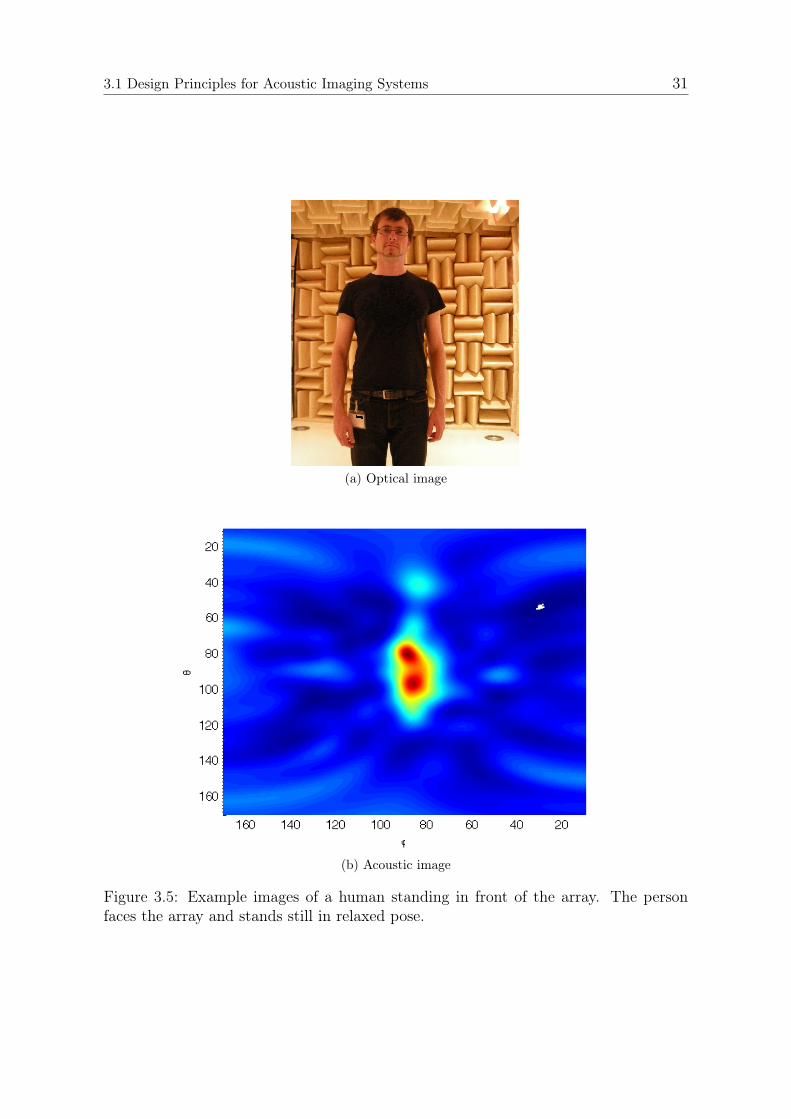
spread of (∆θ; ∆φ) = (13; 32)◦ from the array’s perspective. While the main peak isclearly the direct reflection from the front side of the box, one can also see echoes fromthe lateral edges as well as the bottom edge. The echo from the upper edge overlapswith the direct reflection. Echoes from the region θ > 115◦ do not belong to the object,but are attenuated echoes from the pedestal. In Figure 3.5, we give an example of anacoustic image of a human standing in front of the array. It can be seen that themain reflective areas from the person are the head and torso. Depending on the poseand orientation, the shape of the torso echo will change while the head echo is lessdependent on the exact pose. Additionally, arm and legs reflect echoes back to thearray if the person moves them in a way that they have reflective areas orthogonal thedirect line towards the array.
3.1 Design Principles for Acoustic Imaging Systems 29
(a) Optical image of the reference pole.
(b) Acoustic image of the pole with a smooth surface.
(c) Acoustic image of the pole with a rough surface.
Figure 3.3: Example images of a reference pole object according to [ISO10]. Thesame object is shown with different surfaces. The acoustic images show the significantchanges between specular scattering on a smooth surface and diffuse scattering fromthe rough surface.
30 Chapter 3: Design of Acoustic Imaging Systems
Figure 3.4: Image of a cuboid on a pedestal.
3.1 Design Principles for Acoustic Imaging Systems 31
(a) Optical image
(b) Acoustic image
Figure 3.5: Example images of a human standing in front of the array. The personfaces the array and stands still in relaxed pose.
32 Chapter 3: Design of Acoustic Imaging Systems
3.2 Calibration Techniques
The performance of sensor arrays is well-known to be sensitive to errors or uncertaintiesin the model of the array manifold (see e.g. [VS94b,VS94a,SK92]). In practice, manyof the array’s characteristics can differ from their nominal values and are not preciselyknown a priori, e.g., due to imperfections in the hardware, manufacturing tolerances,mounting errors, etc. Thus, the sensor array is affected by gain and phase differences ofthe sensors, position errors and imbalances in receiver electronics that alter the arraymanifold. In order to account for these inevitable errors and production tolerances,every practical sensor array has to be calibrated such that the mismatch betweenassumptions and reality can be reduced. On the other hand, if the desired accuracyof the calibrated system is known, it may be possible to relax the tolerances requiredin production and compensate for that with the calibration procedure, potentiallyresulting in a manufacturing cost reduction. In this chapter, we will formulate thecalibration problem and illustrate the common approaches in the literature. We willthen describe a calibration method which is specifically suited for acoustic arrays andallows to compensate position errors with low complexity. We will present resultsobtained using simulations and real data measurements and discuss the performancein relation to other calibration methods.
3.2.1 Fundamentals
Following the standard signal model from Section 2.1.1, the output of the array can bedescribed as
x(t) = AS(t) + σnI,
where s(t) describes the signal vector,A is the array response matrix and σnI describesthe uniform noise with power σ2
n at each sensor. Since A models the spatial sensitivityof the overall array, the accuracy of the assumed model is crucial for the performanceof any array signal processing techniques. The theoretical model displayed here differsfrom reality in that it assumes ideal isotropic, homogeneous sensor elements, perfectsynchronization between the elements and no coupling effects. These assumptions arerarely true in practice due to manufacturing tolerances and imperfections. While itis possible to adjust the model in some aspects based on some nominal knowledgeabout the hardware, the specific properties of the single sensors vary and cannot bemodeled accurately a priori. As a consequence, different sources of error arise whenthe nominal array response matrix is used. Some of these errors result in direction-independent offset errors, some in direction-dependent changes of the model. The true
3.2 Calibration Techniques 33
array manifold at(k) is then unknown and has to be estimated. This is typically doneusing offline measurements with calibration sources. These sources send known signalsfrom different directions. Based on the widely applied approach in [PK91], we modelthe deviations of the true array manifold from the nominal model by the use of acalibration matrix Q such that
at(k) = Qa(k) . (3.1)
Thus, finding the true array manifold can be reduced to finding a good estimate ofQ, based on measurements from D calibration sources from known directions (θd, φd)
with d = 1, . . . , D. We denote the whole set of calibration angles by (θcal, φcal). Thisapproach is termed offline calibration and serves as a tool to correct static errors in thearray before its operation. Additionally, online calibration is based on the incomingsignals during operation and can correct dynamic errors during operation, e.g., dueto temperature changes. However, due to the lower amount of information typicallyavailable during online operation, these methods can not compensate larger errors.Depending on the types of present errors,Q has to be modeled as a function of directionor can be constrained in its form, e.g., if no coupling is present, Q is a diagonal matrix.If position errors are present, its coefficients are functions of the direction angles:
Q(k) = Q(θ, φ) = diag {q1(θ, φ), . . . , qN(θ, φ)} . (3.2)
Under those assumptions, we seek the optimalQ(θ, φ) in order to solve the least-squaresproblem
minQ(θ,φ)
ε = ||At(θ, φ)−Q(θ, φ)A(θ, φ)||F (3.3)
for all directions, where || · ||F stands for the Frobenius norm. Let us repeat here thatthe dth column of A describes the array response vector for the dth source and is ofthe form
a(kd,ψ) =
ejkTd p1
...ejk
Td pN
, (3.4)
with ψ = vec{p1,p2, . . . ,pN} denoting a vector with the stacked position vectors pnof all N sensors. The true array response for the calibration directions At(θcal, φcal)
can be estimated by determining the principal eigenvector of the empirical covariancematrix R of the data received from that single source [PK91].
In this work, we focus on offline calibration because the cheap production of the sensorsintroduces several errors which require a precise calibration. On the other hand, dy-namic errors in acoustic imaging are not severely affecting the performance of the arrayand are neglected here. There exists a wealth of approaches to the problem of offline

34 Chapter 3: Design of Acoustic Imaging Systems
calibration of a sensor array. They can be discriminated with respect to their assump-tions about both the types of errors as well as their assumed effects on the array model.Methods which compensate only for direction-independent errors are global techniques,as they estimate Q as single matrix valid for all directions. Local calibration methods,on the other hand, can take also direction-dependent errors into account, which resultsin a correction matrix that is also a function of direction. While both global and localmethods directly estimate the calibration matrix, there are also approaches which tryto estimate some parameters of the array , e.g., the sensor positions, parametricallybased on some model [Vib10]. Those techniques can often be combined with local orglobal techniques.
3.2.2 Global Calibration Techniques
As just described above, global calibration approaches assume that all errors presentin the array can be corrected by a global calibration matrix which is not a functionof the angles θ and φ. Such techniques can account for gain and phase offset errorsof the single elements, but, e.g., not for deviations of the single sensor beam-patterns.Additionally, it is mostly assumed in the literature that inter-element coupling is alsodirection-independent and, thus, can also be corrected (e.g. [PK91,DLX00]). Globalmethods estimate the calibration matrix by solving an optimization problem under theabove assumptions as
Q = arg minQ||QA(θcal, φcal)− At(θcal, φcal)Ξ||F , (3.5)
with Ξ being a complex weighting matrix. For Ξ = I, this leads to the solution [PK91]:
Q = At(θcal, φcal)A†(θcal, φcal), (3.6)
where A† = AH(AAH)−1 is the Moore-Penrose pseudo-inverse of the ideal array re-sponse matrix A. If no mutual coupling is present, this matrix will be diagonal and thesolution is always unique. If coupling is affecting the sensors, the number of availablecalibration sources D must be larger than the number of elements N in order to obtaina unique solution for Q. By choosing the weighting matrix Ξ 6= I, one can emphasizeand possibly improve the classification for specific regions, see e.g. [LVL07]. An itera-tive procedure for the calculation of Q, that does not require matrix inversion has beengiven in [Hun00]. One general advantage of global calibration methods is that one canpreprocess the array data with the inverse global calibration matrix before applyingthe beamforming algorithm. Moreover, only a single matrix is stored.
3.2 Calibration Techniques 35
3.2.3 Local Calibration Techniques
Although global methods can compensate offset errors and compensate couplingbetween the single array elements, the techniques fail completely when direction-dependent errors are affecting the array. Thus, they are computationally attractive,but local methods are needed as soon as there is uncertainty about position errors orother direction dependent The aim of local calibration is to find a correction matrixQ(θ, φ) which is a function of direction, such that
at(θ, φ) = Q(θ, φ)a(θ, φ) . (3.7)
Typically, the calibration data is weighted and the weights depend on the directionof interest. For example, the algorithm proposed in [LLV06] uses the classical ideasof Pierre and Kaveh [PK91], but a direction dependent weight matrix is added whichmakes it possible to take direction dependent errors into account. The method doesnot assume prior knowledge about the errors, which makes it interesting in cases wherethe presence of errors is unknown and one has to assume that several types of directiondependent errors could be present. Q(θ, φ) is calculated for every direction of interest,which means that the correction matrix is a function of the angle. The optimal Q fordirection (θ, φ) in a weighted least squares sense is given by:
Q(θ, φ) = arg minQ||At((θ, φ)cal)−QAi((θ, φ)cal)W
1/2(θ, φ)||F ,
where (θ, φ) is the current angle to be calibrated and W(θ, φ) is a diagonal weightingmatrix for direction (θ, φ) with D non-zero elements. Since each correction matrixQ(θ, φ) is calculated for a single direction, it is sufficient to model Q as a diagonalmatrix in order to capture any deviation from the nominal model.The diagonal elements of Q(θ, φ) can be calculated using the following equation:
qn(θ, φ) =
∑Dd=1 a
∗ndwd(θ, φ)at,nd∑D
d=1 a∗ndwd(θ, φ)and
, n = 1, ..., N.
The weights wd(θ, φ) in W should have the property that the calibration data fromangles in the set (θ, φ)cal,j which are close to (θ, φ) have strong weight and directionsfurther away are less significant. Therefore, the chosen weighting function in [LLV06] iswj(θ, φ) = exp(−h · ||(θ, φ)cal,j − (θ, φ)||2). The bandwidth parameter h determines theamount of smoothing. A large bandwidth results in a narrow weighting function, givinglow weight to more distant data. A too narrow weight function will give a worse inter-polation between the calibration angles and less reduction of noise in the calibrationdata. On the other hand, choosing a small bandwidth will result in a DOA estimate
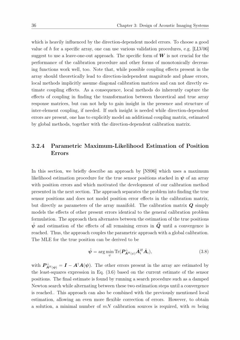
36 Chapter 3: Design of Acoustic Imaging Systems
which is heavily influenced by the direction-dependent model errors. To choose a goodvalue of h for a specific array, one can use various validation procedures, e.g. [LLV06]suggest to use a leave-one-out approach. The specific form of W is not crucial for theperformance of the calibration procedure and other forms of monotonically decreas-ing functions work well, too. Note that, while possible coupling effects present in thearray should theoretically lead to direction-independent magnitude and phase errors,local methods implicitly assume diagonal calibration matrices and can not directly es-timate coupling effects. As a consequence, local methods do inherently capture theeffects of coupling in finding the transformation between theoretical and true arrayresponse matrices, but can not help to gain insight in the presence and structure ofinter-element coupling, if needed. If such insight is needed while direction-dependenterrors are present, one has to explicitly model an additional coupling matrix, estimatedby global methods, together with the direction-dependent calibration matrix.
3.2.4 Parametric Maximum-Likelihood Estimation of PositionErrors
In this section, we briefly describe an approach by [NS96] which uses a maximumlikelihood estimation procedure for the true sensor positions stacked in ψ of an arraywith position errors and which motivated the development of our calibration methodpresented in the next section. The approach separates the problem into finding the truesensor positions and does not model position error effects in the calibration matrix,but directly as parameters of the array manifold. The calibration matrix Q simplymodels the effects of other present errors identical to the general calibration problemformulation. The approach then alternates between the estimation of the true positionsψ and estimation of the effects of all remaining errors in Q until a convergence isreached. Thus, the approach couples the parametric approach with a global calibration.The MLE for the true position can be derived to be
ψ = arg minψ
Tr(P⊥AH(ψ)AHt At), (3.8)
with P⊥AH(ψ) = I −A†A(ψ). The other errors present in the array are estimated bythe least-squares expression in Eq. (3.6) based on the current estimate of the sensorpositions. The final estimate is found by running a search procedure such as a dampedNewton search while alternating between these two estimation steps until a convergenceis reached.. This approach can also be combined with the previously mentioned localestimation, allowing an even more flexible correction of errors. However, to obtaina solution, a minimal number of mN calibration sources is required, with m being

3.2 Calibration Techniques 37
the number of dimensions in which the positions are disturbed, e.g., if the positionsare perturbed on a plane, m = 2. This constraint is of importance specifically forthe calibration of 2D arrays where significantly more array elements are employed.Furthermore, the approach does not model the effect of position errors explicitly, itsimply corrects the errors.
3.2.5 Proposed Low-complexity Estimation Procedure
The requirement of a minimal number of calibration sources is not of significance forsmall one-dimensional (1D) arrays, but can easily become perturbing for larger 2Darrays. To overcome these limitations, we present in this section an approach thatexplicitly models the phase effect of position errors on the array and does not requirea minimal number of sources that depends on the array size. Assuming that eachposition vector pn is affected by an additive random vector ρn, we can derive that theresulting additive phase error is proportional to the components of ρ because for anydirection (θ, φ) we have
at(k) = at(θ, φ) =
ejkTd (p1+ρ1)
...ejk
Td (pN+ρN )
= Q(θ, φ)a(θ, φ) . (3.9)
Thus, the position errors are included in the main diagonal of Q(θ, φ) and result in aphase shift
�qn(θ, φ) = kTρn (3.10)
for a signal with wave vector k. Thus, using calibration sources from known directions(φd), we can estimate the position errors under use of the coefficients qn. The estimatorfor each sensor can then simply be obtained by a least-squares formulation as
ρn = arg minρn||�qn − kTρn||F , n = 1, . . . , N . (3.11)
Generally, the coefficients qn can be estimated as (weighted) sum over all calibrationsources (see [PK91,LLV06]):
qn =1
D
D∑d=1
at(θd, φd)
a(θd, φd), n = 1, . . . , N . (3.12)
In contrast, using eq. (3.12) in Eq. (3.11) removes the need for a minimal number ofcalibration sources and principally allows a position error estimate ρn based already
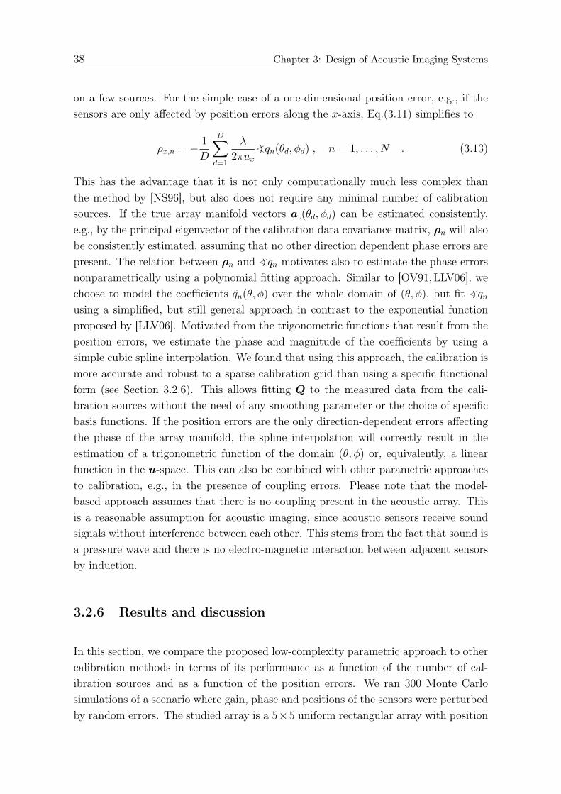
38 Chapter 3: Design of Acoustic Imaging Systems
on a few sources. For the simple case of a one-dimensional position error, e.g., if thesensors are only affected by position errors along the x-axis, Eq.(3.11) simplifies to
ρx,n = − 1
D
D∑d=1
λ
2πux�qn(θd, φd) , n = 1, . . . , N . (3.13)
This has the advantage that it is not only computationally much less complex thanthe method by [NS96], but also does not require any minimal number of calibrationsources. If the true array manifold vectors at(θd, φd) can be estimated consistently,e.g., by the principal eigenvector of the calibration data covariance matrix, ρn will alsobe consistently estimated, assuming that no other direction dependent phase errors arepresent. The relation between ρn and �qn motivates also to estimate the phase errorsnonparametrically using a polynomial fitting approach. Similar to [OV91,LLV06], wechoose to model the coefficients qn(θ, φ) over the whole domain of (θ, φ), but fit �qnusing a simplified, but still general approach in contrast to the exponential functionproposed by [LLV06]. Motivated from the trigonometric functions that result from theposition errors, we estimate the phase and magnitude of the coefficients by using asimple cubic spline interpolation. We found that using this approach, the calibration ismore accurate and robust to a sparse calibration grid than using a specific functionalform (see Section 3.2.6). This allows fitting Q to the measured data from the cali-bration sources without the need of any smoothing parameter or the choice of specificbasis functions. If the position errors are the only direction-dependent errors affectingthe phase of the array manifold, the spline interpolation will correctly result in theestimation of a trigonometric function of the domain (θ, φ) or, equivalently, a linearfunction in the u-space. This can also be combined with other parametric approachesto calibration, e.g., in the presence of coupling errors. Please note that the model-based approach assumes that there is no coupling present in the acoustic array. Thisis a reasonable assumption for acoustic imaging, since acoustic sensors receive soundsignals without interference between each other. This stems from the fact that sound isa pressure wave and there is no electro-magnetic interaction between adjacent sensorsby induction.
3.2.6 Results and discussion
In this section, we compare the proposed low-complexity parametric approach to othercalibration methods in terms of its performance as a function of the number of cal-ibration sources and as a function of the position errors. We ran 300 Monte Carlosimulations of a scenario where gain, phase and positions of the sensors were perturbedby random errors. The studied array is a 5×5 uniform rectangular array with position

3.2 Calibration Techniques 39
errors uniformly distributed in a circle of radius ||ρ|| = 0.2λ on the aperture around thenominal positions. Additionally, the gain and phase of the sensors are affected by uni-formly distributed random variables such that the true array response of the nth sensorat,n can be expressed by the nominal response an, a random variable ζ representingmagnitude errors, and another random variable η representing phase errors:
at,n = (|an|(1 + ζ))ej�(an)+η, (3.14)
ζ ∼ U(−0.15, 0.15),
η ∼ U(0, π/6) .
Because we are interested only in acoustic arrays in this work, we assume that thereis no coupling present. The calibration sources are placed uniformly across the grid,although this is not required. In Figure 3.6, the approach is compared to other methodsfor a varying number of available calibration sources. To vary the number of calibrationsources, we uniformly increase the density of the calibration grid. Performance ismeasured by the resulting calibration error ε in decibel. It is illustrated that the globalmethod by [Hun00] fails to model the present errors independent of the number ofavailable sources and is only slightly correcting the nominal model as expected. Thelocal methods perform better with an increasing number of calibration sources becausethey can model the array manifold more accurately in all directions the more dense thecalibration grid becomes. While the approach by [LLV06] can correct the error partly,it performs worse than all other local methods. The computationally more complexmethod by [OV91] uses a rather generic polynomial functional to model the arraymanifold which allows a better calibration. Furthermore, we can see that fitting Qusing spline interpolation alone (denoted by "Q-space”) already outperforms the otherlocal calibration methods, but is worse than the method of [NS96] which is able toalmost perfectly model the true array manifold if the condition on the minimal numberof sources is fulfilled. When Q-space fitting is combined with parametric estimation asproposed (denoted by ParamLocal), we see that the performance is equal to the oneof [NS96]. Additionally, it is capable to model the errors accurately even for only tencalibration sources because it does not require a minimal number of calibration sources.We want to emphasize that ε should not be interpreted as a measure for DOA estimationaccuracy in array problems. However, it is meaningful to compare the methods interms of this correction error as it is derived from the initial problem formulation.Similar results are obtained when the methods are compared with respect to the co-linearity between the true and calibrated array response. The order in performance isequal, however, the gap between the parametric and nonparametric approaches is lessvisible. In Figure 3.7, the performance of the different algorithms is evaluated whenthe effect of the position errors is varied from 0.01λ to 0.2λ. We see that both theproposed method and the method of [NS96] are able to correct the positions in every
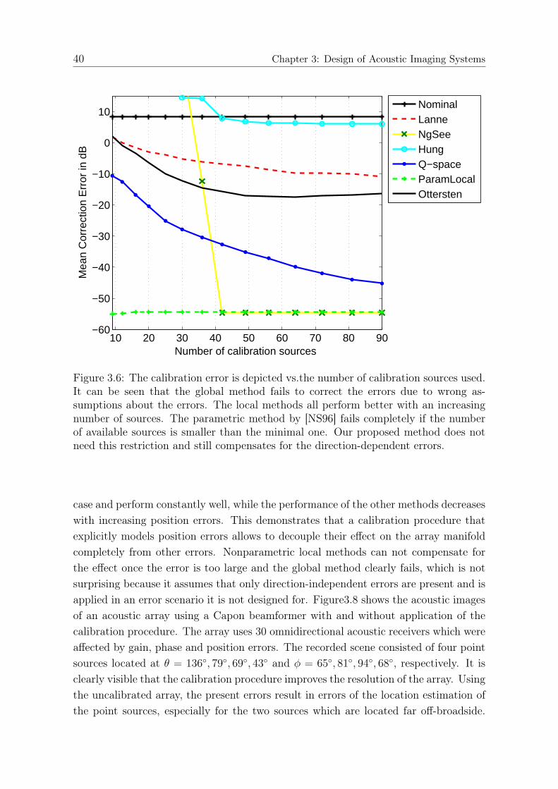
40 Chapter 3: Design of Acoustic Imaging Systems
10 20 30 40 50 60 70 80 90−60
−50
−40
−30
−20
−10
0
10
Number of calibration sources
Mea
n C
orre
ctio
n E
rror
in d
B
NominalLanneNgSeeHungQ−spaceParamLocalOttersten
Figure 3.6: The calibration error is depicted vs.the number of calibration sources used.It can be seen that the global method fails to correct the errors due to wrong as-sumptions about the errors. The local methods all perform better with an increasingnumber of sources. The parametric method by [NS96] fails completely if the numberof available sources is smaller than the minimal one. Our proposed method does notneed this restriction and still compensates for the direction-dependent errors.
case and perform constantly well, while the performance of the other methods decreaseswith increasing position errors. This demonstrates that a calibration procedure thatexplicitly models position errors allows to decouple their effect on the array manifoldcompletely from other errors. Nonparametric local methods can not compensate forthe effect once the error is too large and the global method clearly fails, which is notsurprising because it assumes that only direction-independent errors are present and isapplied in an error scenario it is not designed for. Figure3.8 shows the acoustic imagesof an acoustic array using a Capon beamformer with and without application of thecalibration procedure. The array uses 30 omnidirectional acoustic receivers which wereaffected by gain, phase and position errors. The recorded scene consisted of four pointsources located at θ = 136◦, 79◦, 69◦, 43◦ and φ = 65◦, 81◦, 94◦, 68◦, respectively. It isclearly visible that the calibration procedure improves the resolution of the array. Usingthe uncalibrated array, the present errors result in errors of the location estimation ofthe point sources, especially for the two sources which are located far off-broadside.
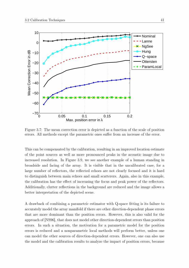
3.2 Calibration Techniques 41
0 0.05 0.1 0.15 0.2−70
−60
−50
−40
−30
−20
−10
0
10
Max. position error in λ
Mea
n C
orre
ctio
n E
rror
in d
B
NominalLanneNgSeeHungQ−spaceOtterstenParamLocal
Figure 3.7: The mean correction error is depicted as a function of the scale of positionerrors. All methods except the parametric ones suffer from an increase of the error.
This can be compensated by the calibration, resulting in an improved location estimateof the point sources as well as more pronounced peaks in the acoustic image due toincreased resolution. In Figure 3.9, we see another example of a human standing inbroadside and facing of the array. It is visible that in the uncalibrated case, for alarge number of reflectors, the reflected echoes are not clearly focused and it is hardto distinguish between main echoes and small scatterers. Again, also in this example,the calibration has the effect of increasing the focus and peak power of the reflectors.Additionally, clutter reflections in the background are reduced and the image allows abetter interpretation of the depicted scene.
A drawback of combining a parametric estimator with Q-space fitting is its failure toaccurately model the array manifold if there are other direction-dependent phase errorsthat are more dominant than the position errors. However, this is also valid for theapproach of [NS96], that does not model other direction-dependent errors than positionerrors. In such a situation, the motivation for a parametric model for the positionerrors is reduced and a nonparametric local methods will perform better, unless onecan model the other sources of direction-dependent errors. However, one can also usethe model and the calibration results to analyze the impact of position errors, because

42 Chapter 3: Design of Acoustic Imaging Systems
of its previously derived known effect on the array response. Due to the trigonometricrelation wave vector and phase effect of the position errors, the interpolation betweenmeasured calibration sources leads to trigonometric functions with respect to directionfor all array elements affected by a position error. As described above, the amplitudeof these trigonometric functions is proportional to the magnitude of the error.
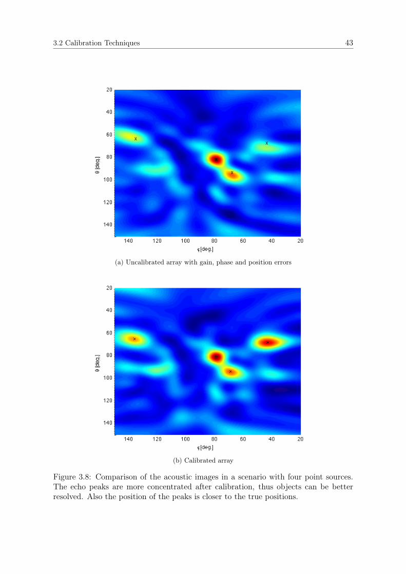
3.2 Calibration Techniques 43
(a) Uncalibrated array with gain, phase and position errors
(b) Calibrated array
Figure 3.8: Comparison of the acoustic images in a scenario with four point sources.The echo peaks are more concentrated after calibration, thus objects can be betterresolved. Also the position of the peaks is closer to the true positions.
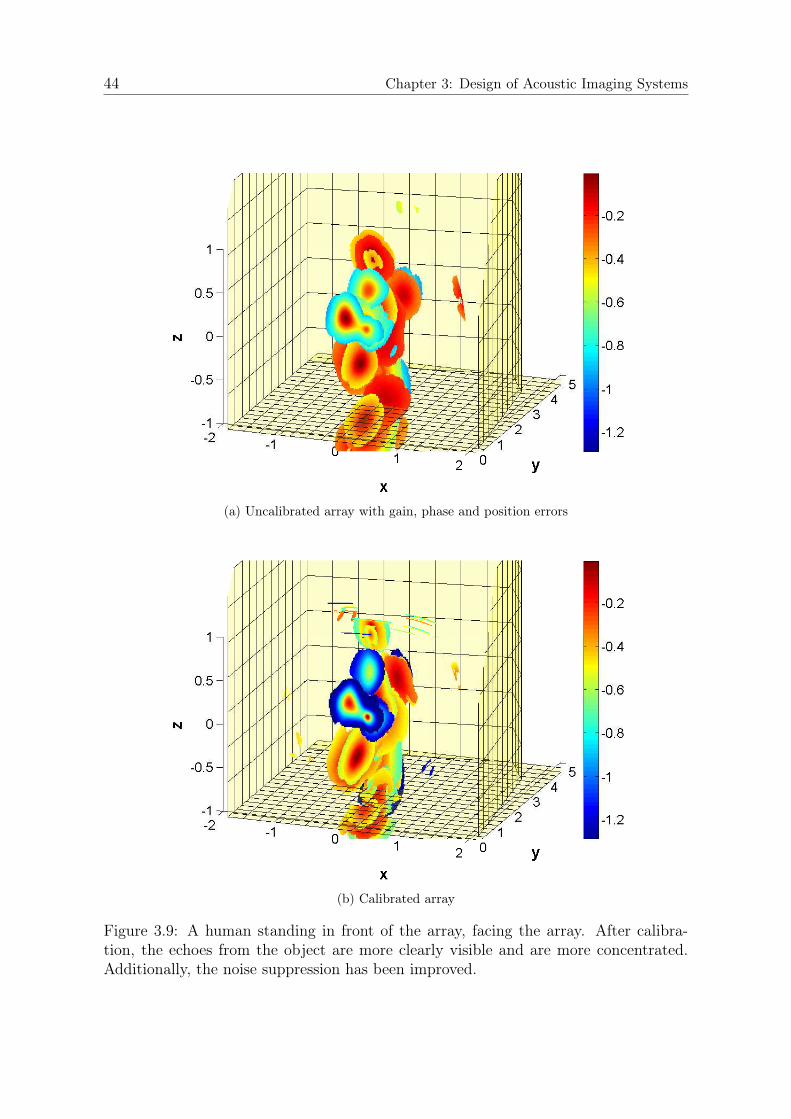
44 Chapter 3: Design of Acoustic Imaging Systems
(a) Uncalibrated array with gain, phase and position errors
(b) Calibrated array
Figure 3.9: A human standing in front of the array, facing the array. After calibra-tion, the echoes from the object are more clearly visible and are more concentrated.Additionally, the noise suppression has been improved.
45
Chapter 4
Sparse Array Design
4.1 Introduction
As discussed in Chapter 1, acoustic imaging for robotic applications requires cheaphardware, but still demands for good spatial resolution and noise suppression. Es-pecially the use of 2D arrays for 3D imaging is challenging, e.g. the high num-ber of sensors and therefore active channels employed in such systems, leads to in-creased hardware and computational costs. This motivates the use of 2D sparse ar-rays which approximate the beam-pattern of a fully populated array using a lowernumber of sensors. However, the geometry of the array has to be optimized, asit fundamentally influences all performance parameters. There have been numerousapproaches to design sparse 1D and 2D arrays using single- and multi-objective op-timization techniques where Half-Power-Beam-Width (HPBW) and Side-Lobe-Level(SLL) are optimized. Common approaches design sparse arrays by either thin-ning a full array [AH02, AH02, HAIH01, Tru99, AHW+97, KS91, Kop92] or randomlyplacing a fixed number of sensors, sometimes under some geometrical constraints[JRS07,OM05,Ruf93,RL75]. These approaches allow to obtain good results, but relyon the evaluation of a cost function over a large search space and involve subjectiveweighting of the individual goals. To find good solutions, these methods require thecreation of a large number of possible candidates from which one has to be selected.This allows little or no control over the properties of a found solution. In this chapter,we discuss design methods for sparse 2D arrays that are suitable for acoustic imagingapplications, e.g., obstacle detection in robotics, or medical imaging diagnosis. Due tothe slow wave propagation speed as well as hardware constraints, systems operating inair transmit in broadcast mode and therefore require a receiver beam-pattern withoutgrating lobes.1 The approach presented in this chapter enables the design of highlysparse 2D arrays that exhibit low SLLs. Additionally, direct control over the trade-offbetween sparsity and SLL is achieved. The approach is based on the theory of mini-mum redundancy and employs an iterative procedure that populates the array aperturewith additional sensor elements. The criterion for the placement of additional sensoris formulated such that the co-array is manipulated to allow a good approximation of
1In active systems that employ both transmit and receive beamforming, e.g. in medical imaging,it is common to optimize the two-way-beam-pattern of the array, i.e. grating lobes are allowedfor the transmission beam-pattern and are suppressed in receiving mode by controlled nulling (seee.g. [LTB98]).
46 Chapter 4: Sparse Array Design
the performance of a full array. This allows to choose a suitable combination of SLLand sparsity while exhibiting a low computational complexity. These advantages comeat the cost of an altered mainlobe shape which can become quasi-convex.
4.2 Problem Formulation
Based on the signal model presented in Section 2.1.1, we formulate the sparse array de-sign problem in the context of acoustic imaging as the problem of finding a sparse arraywith κ elements that performs well in terms of object resolution and noise suppression.The reference of performance is the beam-pattern of a full Uniform Rectangular Arraywith N = Nx × Nz elements with λ/2-spacing. Our goal is to reduce the number ofsensor elements in this 2D planar array while retaining the resolution and suppressioncapabilities of the corresponding URA with respect to λ, such that the spatial powerspectrum estimate is still consistent2. In other terms, we want to approximate thebeam-pattern of an URA by the use of a nonuniform sparse array with only κ < N
elements on the same aperture for all possible steering angles kl. For the imagingapplications of interest, we measure performance in terms of the SLL and mainlobewidth of the beam-pattern of a Bartlett beamformer as well as the sparsity of the usedarray, measured by the thinning factor κ/N . The SLL is defined as the distance be-tween the maximum value in the mainlobe of the beam-pattern and the second-largestmaximum value. Additionally, grating lobes have to be avoided by all cost as they leadto spurious peaks in the resulting images. Note that while the Integrated-SideLobe-Ratio (ISLR) is used for evaluation in some applications, we do not use it here becauseit is less important in the application of interest. This is due to the fact that we dealwith situations where there are only relatively few scatterers simultaneously presentin the image. Reducing κ can be interpreted as a measure of compressive spatial 2Dsampling. In this context, we can say that we are interested to find the transformationfunction Γ(·) which transforms the beam-pattern of the URA into the beam-pattern ofthe sparse array such that certain properties of the image obtained by the full, dense ar-ray are the desired parameters to be reliably estimated using the sparse sampling. Forexample, using Bartlett’s beamformer, the beam-pattern of the sparse array looking atdirection kl is
BS(k)|kl =wHS (kl) · aS(k) (4.1)
=1
κ
κ∑i=1
ai(kl)HaS,i(k) , (4.2)
2The consistency of power spectra based on nonuniform sampling is proved in [Mar86,MC90].
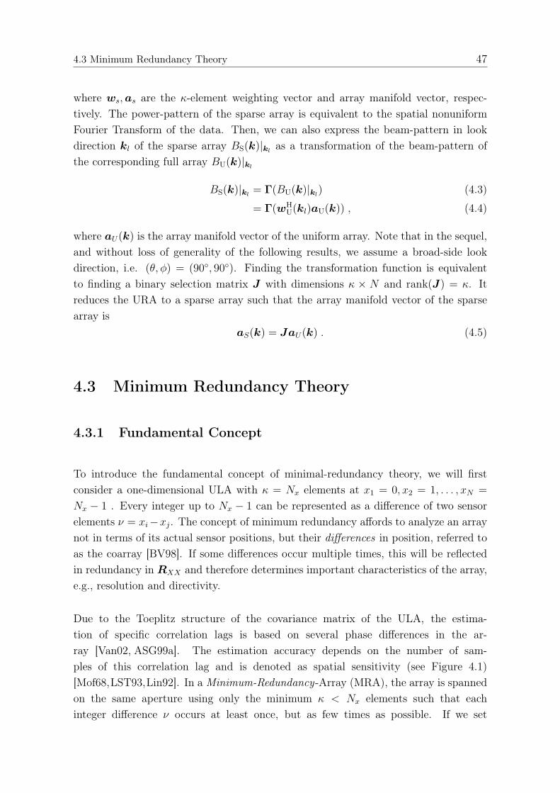
4.3 Minimum Redundancy Theory 47
where ws,as are the κ-element weighting vector and array manifold vector, respec-tively. The power-pattern of the sparse array is equivalent to the spatial nonuniformFourier Transform of the data. Then, we can also express the beam-pattern in lookdirection kl of the sparse array BS(k)|kl as a transformation of the beam-pattern ofthe corresponding full array BU(k)|kl
BS(k)|kl = Γ(BU(k)|kl) (4.3)
= Γ(wHU(kl)aU(k)) , (4.4)
where aU(k) is the array manifold vector of the uniform array. Note that in the sequel,and without loss of generality of the following results, we assume a broad-side lookdirection, i.e. (θ, φ) = (90◦, 90◦). Finding the transformation function is equivalentto finding a binary selection matrix J with dimensions κ × N and rank(J) = κ. Itreduces the URA to a sparse array such that the array manifold vector of the sparsearray is
aS(k) = JaU(k) . (4.5)
4.3 Minimum Redundancy Theory
4.3.1 Fundamental Concept
To introduce the fundamental concept of minimal-redundancy theory, we will firstconsider a one-dimensional ULA with κ = Nx elements at x1 = 0, x2 = 1, . . . , xN =
Nx − 1 . Every integer up to Nx − 1 can be represented as a difference of two sensorelements ν = xi−xj. The concept of minimum redundancy affords to analyze an arraynot in terms of its actual sensor positions, but their differences in position, referred toas the coarray [BV98]. If some differences occur multiple times, this will be reflectedin redundancy in RXX and therefore determines important characteristics of the array,e.g., resolution and directivity.
Due to the Toeplitz structure of the covariance matrix of the ULA, the estima-tion of specific correlation lags is based on several phase differences in the ar-ray [Van02, ASG99a]. The estimation accuracy depends on the number of sam-ples of this correlation lag and is denoted as spatial sensitivity (see Figure 4.1)[Mof68,LST93,Lin92]. In a Minimum-Redundancy-Array (MRA), the array is spannedon the same aperture using only the minimum κ < Nx elements such that eachinteger difference ν occurs at least once, but as few times as possible. If we set
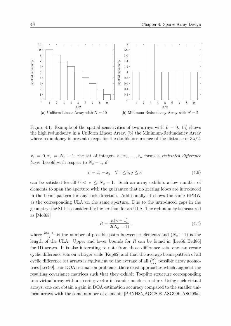
48 Chapter 4: Sparse Array Design
(a) Uniform Linear Array with N = 10 (b) Minimum-Redundancy Array with N = 5
Figure 4.1: Example of the spatial sensitivities of two arrays with L = 9. (a) showsthe high redundancy in a Uniform Linear Array, (b) the Minimum-Redundancy Arraywhere redundancy is present except for the double occurrence of the distance of 3λ/2.
x1 = 0, xκ = Nx − 1, the set of integers x1, x2, . . . , xκ forms a restricted differencebasis [Lee56] with respect to Nx − 1, if
ν = xi − xj ∀ 1 ≤ i, j ≤ κ (4.6)
can be satisfied for all 0 < ν ≤ Nx − 1. Such an array exhibits a low number ofelements to span the aperture with the guarantee that no grating lobes are introducedin the beam pattern for any look direction. Additionally, it shows the same HPBWas the corresponding ULA on the same aperture. Due to the introduced gaps in thegeometry, the SLL is considerably higher than for an ULA. The redundancy is measuredas [Mof68]
R =κ(κ− 1)
2(Nx − 1), (4.7)
where κ(κ−1)2
is the number of possible pairs between κ elements and (Nx − 1) is thelength of the ULA. Upper and lower bounds for R can be found in [Lee56, Bed86]for 1D arrays. It is also interesting to note from those difference sets, one can createcyclic difference sets on a larger scale [Kop92] and that the average beam-pattern of allcyclic difference set arrays is equivalent to the average of all
(Nk
)possible array geome-
tries [Lee99]. For DOA estimation problems, there exist approaches which augment theresulting covariance matrices such that they exhibit Toeplitz structure correspondingto a virtual array with a steering vector in Vandermonde structure. Using such virtualarrays, one can obtain a gain in DOA estimation accuracy compared to the smaller uni-form arrays with the same number of elements [PBNH85,AGGS98,ASG99b,ASG99a].
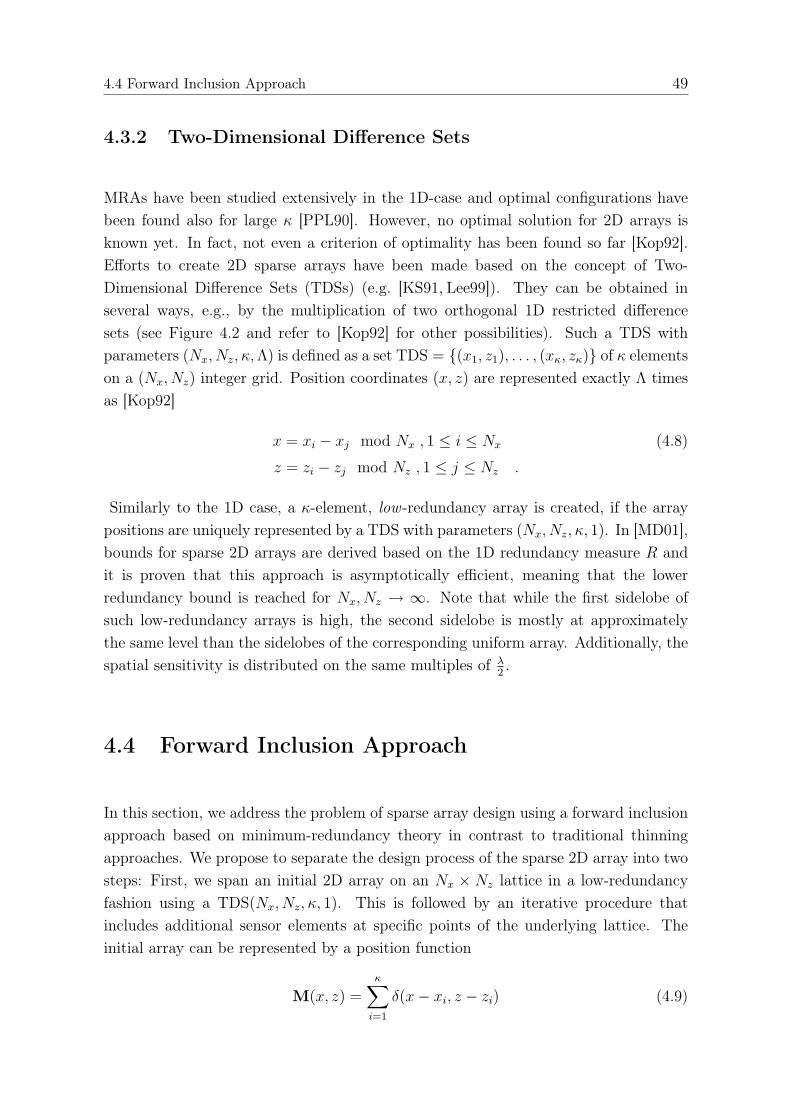
4.4 Forward Inclusion Approach 49
4.3.2 Two-Dimensional Difference Sets
MRAs have been studied extensively in the 1D-case and optimal configurations havebeen found also for large κ [PPL90]. However, no optimal solution for 2D arrays isknown yet. In fact, not even a criterion of optimality has been found so far [Kop92].Efforts to create 2D sparse arrays have been made based on the concept of Two-Dimensional Difference Sets (TDSs) (e.g. [KS91, Lee99]). They can be obtained inseveral ways, e.g., by the multiplication of two orthogonal 1D restricted differencesets (see Figure 4.2 and refer to [Kop92] for other possibilities). Such a TDS withparameters (Nx, Nz, κ,Λ) is defined as a set TDS = {(x1, z1), . . . , (xκ, zκ)} of κ elementson a (Nx, Nz) integer grid. Position coordinates (x, z) are represented exactly Λ timesas [Kop92]
x = xi − xj mod Nx , 1 ≤ i ≤ Nx (4.8)
z = zi − zj mod Nz , 1 ≤ j ≤ Nz .
Similarly to the 1D case, a κ-element, low -redundancy array is created, if the arraypositions are uniquely represented by a TDS with parameters (Nx, Nz, κ, 1). In [MD01],bounds for sparse 2D arrays are derived based on the 1D redundancy measure R andit is proven that this approach is asymptotically efficient, meaning that the lowerredundancy bound is reached for Nx, Nz → ∞. Note that while the first sidelobe ofsuch low-redundancy arrays is high, the second sidelobe is mostly at approximatelythe same level than the sidelobes of the corresponding uniform array. Additionally, thespatial sensitivity is distributed on the same multiples of λ
2.
4.4 Forward Inclusion Approach
In this section, we address the problem of sparse array design using a forward inclusionapproach based on minimum-redundancy theory in contrast to traditional thinningapproaches. We propose to separate the design process of the sparse 2D array into twosteps: First, we span an initial 2D array on an Nx × Nz lattice in a low-redundancyfashion using a TDS(Nx, Nz, κ, 1). This is followed by an iterative procedure thatincludes additional sensor elements at specific points of the underlying lattice. Theinitial array can be represented by a position function
M(x, z) =κ∑i=1
δ(x− xi, z − zi) (4.9)
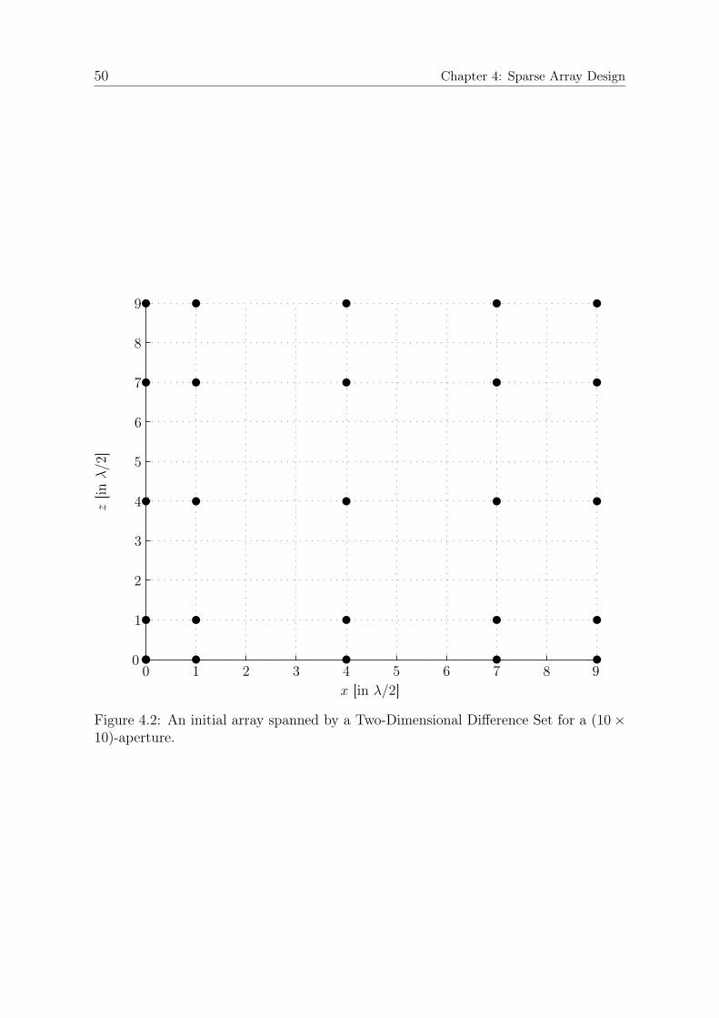
50 Chapter 4: Sparse Array Design
x [in λ/2]
z[in
λ/2
]
0 1 2 3 4 5 6 7 8 90
1
2
3
4
5
6
7
8
9
Figure 4.2: An initial array spanned by a Two-Dimensional Difference Set for a (10×10)-aperture.
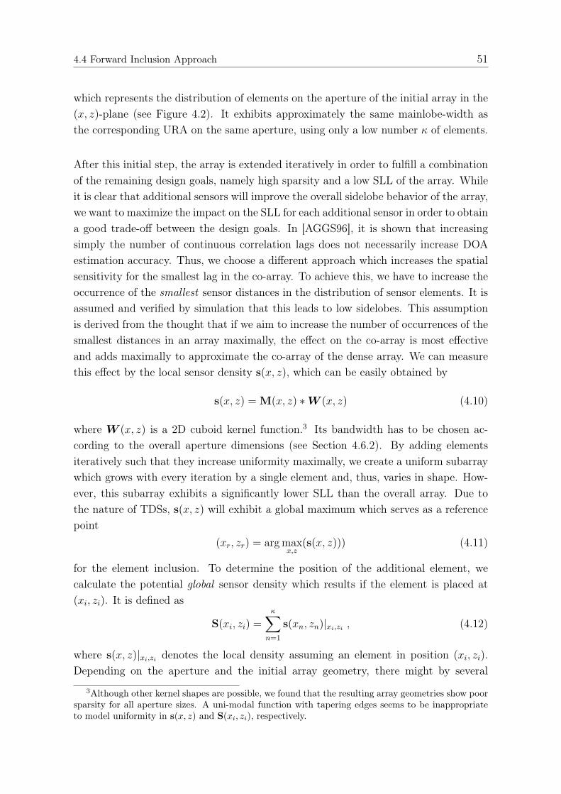
4.4 Forward Inclusion Approach 51
which represents the distribution of elements on the aperture of the initial array in the(x, z)-plane (see Figure 4.2). It exhibits approximately the same mainlobe-width asthe corresponding URA on the same aperture, using only a low number κ of elements.
After this initial step, the array is extended iteratively in order to fulfill a combinationof the remaining design goals, namely high sparsity and a low SLL of the array. Whileit is clear that additional sensors will improve the overall sidelobe behavior of the array,we want to maximize the impact on the SLL for each additional sensor in order to obtaina good trade-off between the design goals. In [AGGS96], it is shown that increasingsimply the number of continuous correlation lags does not necessarily increase DOAestimation accuracy. Thus, we choose a different approach which increases the spatialsensitivity for the smallest lag in the co-array. To achieve this, we have to increase theoccurrence of the smallest sensor distances in the distribution of sensor elements. It isassumed and verified by simulation that this leads to low sidelobes. This assumptionis derived from the thought that if we aim to increase the number of occurrences of thesmallest distances in an array maximally, the effect on the co-array is most effectiveand adds maximally to approximate the co-array of the dense array. We can measurethis effect by the local sensor density s(x, z), which can be easily obtained by
s(x, z) = M(x, z) ∗W (x, z) (4.10)
where W (x, z) is a 2D cuboid kernel function.3 Its bandwidth has to be chosen ac-cording to the overall aperture dimensions (see Section 4.6.2). By adding elementsiteratively such that they increase uniformity maximally, we create a uniform subarraywhich grows with every iteration by a single element and, thus, varies in shape. How-ever, this subarray exhibits a significantly lower SLL than the overall array. Due tothe nature of TDSs, s(x, z) will exhibit a global maximum which serves as a referencepoint
(xr, zr) = arg maxx,z
(s(x, z))) (4.11)
for the element inclusion. To determine the position of the additional element, wecalculate the potential global sensor density which results if the element is placed at(xi, zi). It is defined as
S(xi, zi) =κ∑
n=1
s(xn, zn)|xi,zi , (4.12)
where s(x, z)|xi,zi denotes the local density assuming an element in position (xi, zi).Depending on the aperture and the initial array geometry, there might by several
3Although other kernel shapes are possible, we found that the resulting array geometries show poorsparsity for all aperture sizes. A uni-modal function with tapering edges seems to be inappropriateto model uniformity in s(x, z) and S(xi, zi), respectively.
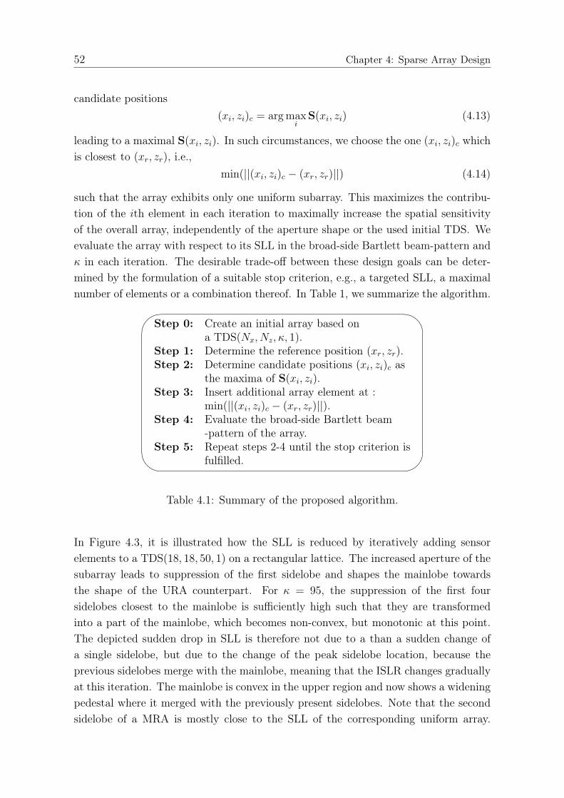
52 Chapter 4: Sparse Array Design
candidate positions(xi, zi)c = arg max
iS(xi, zi) (4.13)
leading to a maximal S(xi, zi). In such circumstances, we choose the one (xi, zi)c whichis closest to (xr, zr), i.e.,
min(||(xi, zi)c − (xr, zr)||) (4.14)
such that the array exhibits only one uniform subarray. This maximizes the contribu-tion of the ith element in each iteration to maximally increase the spatial sensitivityof the overall array, independently of the aperture shape or the used initial TDS. Weevaluate the array with respect to its SLL in the broad-side Bartlett beam-pattern andκ in each iteration. The desirable trade-off between these design goals can be deter-mined by the formulation of a suitable stop criterion, e.g., a targeted SLL, a maximalnumber of elements or a combination thereof. In Table 1, we summarize the algorithm.'
&
$
%
Step 0: Create an initial array based ona TDS(Nx, Nz, κ, 1).
Step 1: Determine the reference position (xr, zr).Step 2: Determine candidate positions (xi, zi)c as
the maxima of S(xi, zi).Step 3: Insert additional array element at :
min(||(xi, zi)c − (xr, zr)||).Step 4: Evaluate the broad-side Bartlett beam
-pattern of the array.Step 5: Repeat steps 2-4 until the stop criterion is
fulfilled.
Table 4.1: Summary of the proposed algorithm.
In Figure 4.3, it is illustrated how the SLL is reduced by iteratively adding sensorelements to a TDS(18, 18, 50, 1) on a rectangular lattice. The increased aperture of thesubarray leads to suppression of the first sidelobe and shapes the mainlobe towardsthe shape of the URA counterpart. For κ = 95, the suppression of the first foursidelobes closest to the mainlobe is sufficiently high such that they are transformedinto a part of the mainlobe, which becomes non-convex, but monotonic at this point.The depicted sudden drop in SLL is therefore not due to a than a sudden change ofa single sidelobe, but due to the change of the peak sidelobe location, because theprevious sidelobes merge with the mainlobe, meaning that the ISLR changes graduallyat this iteration. The mainlobe is convex in the upper region and now shows a wideningpedestal where it merged with the previously present sidelobes. Note that the secondsidelobe of a MRA is mostly close to the SLL of the corresponding uniform array.
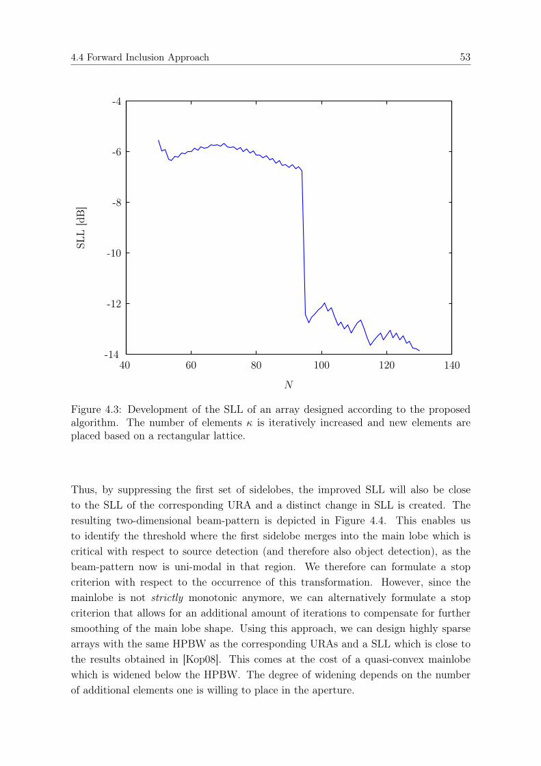
4.4 Forward Inclusion Approach 53
N
SLL
[dB
]
40 60 80 100 120 140-14
-12
-10
-8
-6
-4
Figure 4.3: Development of the SLL of an array designed according to the proposedalgorithm. The number of elements κ is iteratively increased and new elements areplaced based on a rectangular lattice.
Thus, by suppressing the first set of sidelobes, the improved SLL will also be closeto the SLL of the corresponding URA and a distinct change in SLL is created. Theresulting two-dimensional beam-pattern is depicted in Figure 4.4. This enables usto identify the threshold where the first sidelobe merges into the main lobe which iscritical with respect to source detection (and therefore also object detection), as thebeam-pattern now is uni-modal in that region. We therefore can formulate a stopcriterion with respect to the occurrence of this transformation. However, since themainlobe is not strictly monotonic anymore, we can alternatively formulate a stopcriterion that allows for an additional amount of iterations to compensate for furthersmoothing of the main lobe shape. Using this approach, we can design highly sparsearrays with the same HPBW as the corresponding URAs and a SLL which is close tothe results obtained in [Kop08]. This comes at the cost of a quasi-convex mainlobewhich is widened below the HPBW. The degree of widening depends on the numberof additional elements one is willing to place in the aperture.
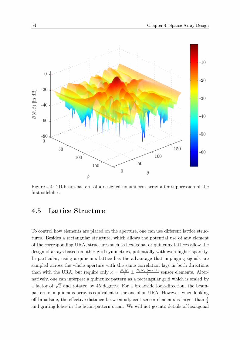
54 Chapter 4: Sparse Array Design
Figure 4.4: 2D-beam-pattern of a designed nonuniform array after suppression of thefirst sidelobes.
4.5 Lattice Structure
To control how elements are placed on the aperture, one can use different lattice struc-tures. Besides a rectangular structure, which allows the potential use of any elementof the corresponding URA, structures such as hexagonal or quincunx lattices allow thedesign of arrays based on other grid symmetries, potentially with even higher sparsity.In particular, using a quincunx lattice has the advantage that impinging signals aresampled across the whole aperture with the same correlation lags in both directionsthan with the URA, but require only κ = NxNz
2± NxNz (mod 2)
2sensor elements. Alter-
natively, one can interpret a quincunx pattern as a rectangular grid which is scaled bya factor of
√2 and rotated by 45 degrees. For a broadside look-direction, the beam-
pattern of a quincunx array is equivalent to the one of an URA. However, when lookingoff-broadside, the effective distance between adjacent sensor elements is larger than λ
2
and grating lobes in the beam-pattern occur. We will not go into details of hexagonal

4.5 Lattice Structure 55
sampling because we found similar performance behavior of the designed arrays forhexagonal lattice structures.
4.5.1 Randomization of Lattices
The main reason for high sidelobes in the beam-patterns of the nonuniform arrays stemsfrom the fact that they are placed on regular grid structures. It is a well-known factthat random placement of sensor elements on the array aperture allows to obtain lowsidelobe levels (e.g. [Lo64, Lo63, Ste72]). The price for this behavior is that sidelobesare positioned in an irregular fashion and there is no control over the properties ofthe beam-pattern possible, such that suitable array layouts can only be obtained byMonte-Carlo simulations. However, a binned randomization of elements around latticenodes allows to achieve lower sidelobes and allows at the same time to a structuredapproach to the problem [HAIH01,Hol00,Hen91]. In order to maintain control over thearray layout, the extent of randomization has to be small, such that the beam-patternis only altered in sidelobe structure, but is still closely related to the beam-patternobtained using strictly lattice nodes. This can be achieved by adding a multivariaterandom variable with limited support to the position vector of each sensor elementsuch that the randomized position of the ith element is described by
p = pi + ρi , 1 ≤ i ≤ κ .
We assume the random variables to be independent and uniformly distributed on theinterval [−λ
4, λ
4] in the x, z-dimensions. Furthermore, ρi is assumed to be deterministic
zero in the second dimension, meaning that the sensors are only moved on the aperturesurface. In Figure 4.5, we show an example of an array geometry on a (10×10)-aperturewith a quincunx grid and binned randomization after several iterations of the proposedalgorithm. The added sensors are restricted to lie inside the depicted boxes around thegrid nodes as described above. The empty circles denote empty nodes in the quincunxgrid which can be used for further iterations by the algorithm. The effect of binnedrandomization on the SLL is illustrated exemplarily in Figure 4.6 where the expectedvalue and the 2, 5%- and 97.5%-percentiles of distribution of the SLL are shown basedon 300 Monte Carlo runs. It can be seen that the average SLL decreases continuously,thus showing the same behavior as in the deterministic case. This is due to the factthat the random variables are distributed with zero mean around the nominal sensorpositions. The variance, however increases as expected because more sensors are addedto the aperture and the variance of the overall beam-pattern of a binned random arrayscales with the number of sensors as
Var{BS(k)} = κ
(1− sinc2(
Nxkxκ2π
)
)(1− sinc2(
Nzkzκ2π
)
),
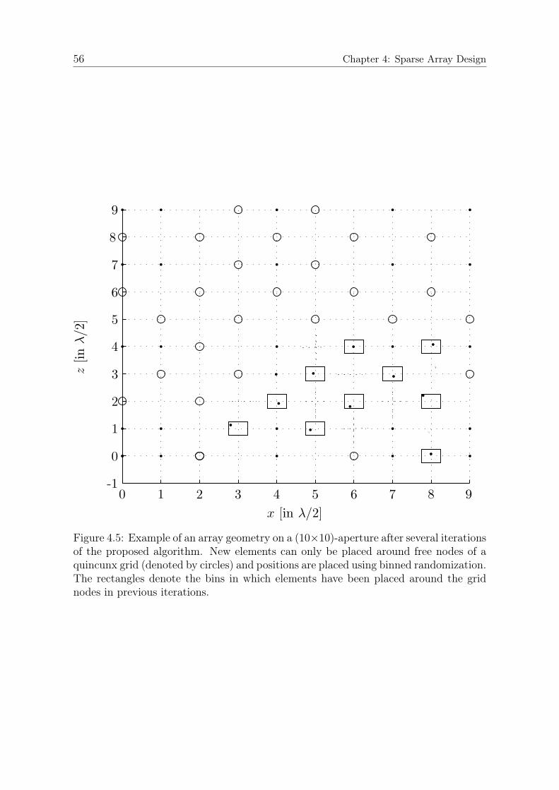
56 Chapter 4: Sparse Array Design
Figure 4.5: Example of an array geometry on a (10×10)-aperture after several iterationsof the proposed algorithm. New elements can only be placed around free nodes of aquincunx grid (denoted by circles) and positions are placed using binned randomization.The rectangles denote the bins in which elements have been placed around the gridnodes in previous iterations.
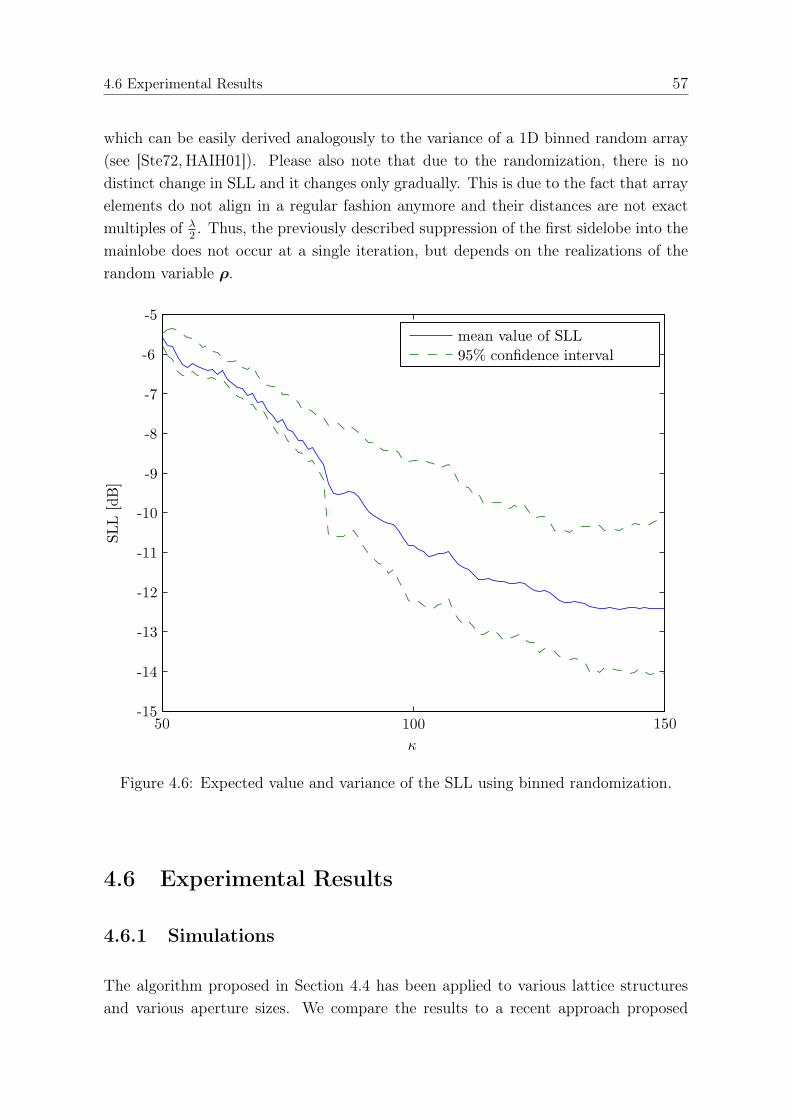
4.6 Experimental Results 57
which can be easily derived analogously to the variance of a 1D binned random array(see [Ste72, HAIH01]). Please also note that due to the randomization, there is nodistinct change in SLL and it changes only gradually. This is due to the fact that arrayelements do not align in a regular fashion anymore and their distances are not exactmultiples of λ
2. Thus, the previously described suppression of the first sidelobe into the
mainlobe does not occur at a single iteration, but depends on the realizations of therandom variable ρ.
Figure 4.6: Expected value and variance of the SLL using binned randomization.
4.6 Experimental Results
4.6.1 Simulations
The algorithm proposed in Section 4.4 has been applied to various lattice structuresand various aperture sizes. We compare the results to a recent approach proposed
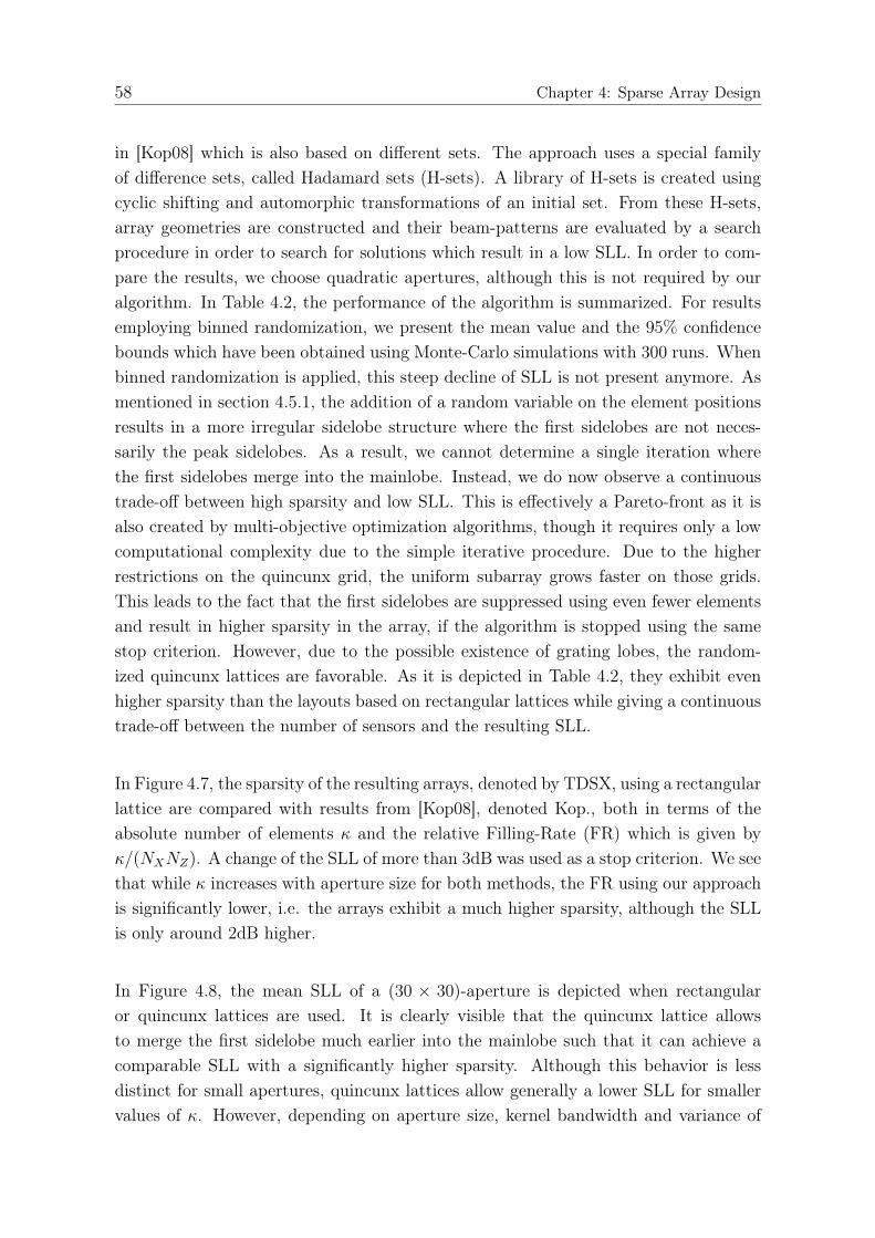
58 Chapter 4: Sparse Array Design
in [Kop08] which is also based on different sets. The approach uses a special familyof difference sets, called Hadamard sets (H-sets). A library of H-sets is created usingcyclic shifting and automorphic transformations of an initial set. From these H-sets,array geometries are constructed and their beam-patterns are evaluated by a searchprocedure in order to search for solutions which result in a low SLL. In order to com-pare the results, we choose quadratic apertures, although this is not required by ouralgorithm. In Table 4.2, the performance of the algorithm is summarized. For resultsemploying binned randomization, we present the mean value and the 95% confidencebounds which have been obtained using Monte-Carlo simulations with 300 runs. Whenbinned randomization is applied, this steep decline of SLL is not present anymore. Asmentioned in section 4.5.1, the addition of a random variable on the element positionsresults in a more irregular sidelobe structure where the first sidelobes are not neces-sarily the peak sidelobes. As a result, we cannot determine a single iteration wherethe first sidelobes merge into the mainlobe. Instead, we do now observe a continuoustrade-off between high sparsity and low SLL. This is effectively a Pareto-front as it isalso created by multi-objective optimization algorithms, though it requires only a lowcomputational complexity due to the simple iterative procedure. Due to the higherrestrictions on the quincunx grid, the uniform subarray grows faster on those grids.This leads to the fact that the first sidelobes are suppressed using even fewer elementsand result in higher sparsity in the array, if the algorithm is stopped using the samestop criterion. However, due to the possible existence of grating lobes, the random-ized quincunx lattices are favorable. As it is depicted in Table 4.2, they exhibit evenhigher sparsity than the layouts based on rectangular lattices while giving a continuoustrade-off between the number of sensors and the resulting SLL.
In Figure 4.7, the sparsity of the resulting arrays, denoted by TDSX, using a rectangularlattice are compared with results from [Kop08], denoted Kop., both in terms of theabsolute number of elements κ and the relative Filling-Rate (FR) which is given byκ/(NXNZ). A change of the SLL of more than 3dB was used as a stop criterion. We seethat while κ increases with aperture size for both methods, the FR using our approachis significantly lower, i.e. the arrays exhibit a much higher sparsity, although the SLLis only around 2dB higher.
In Figure 4.8, the mean SLL of a (30 × 30)-aperture is depicted when rectangularor quincunx lattices are used. It is clearly visible that the quincunx lattice allowsto merge the first sidelobe much earlier into the mainlobe such that it can achieve acomparable SLL with a significantly higher sparsity. Although this behavior is lessdistinct for small apertures, quincunx lattices allow generally a lower SLL for smallervalues of κ. However, depending on aperture size, kernel bandwidth and variance of
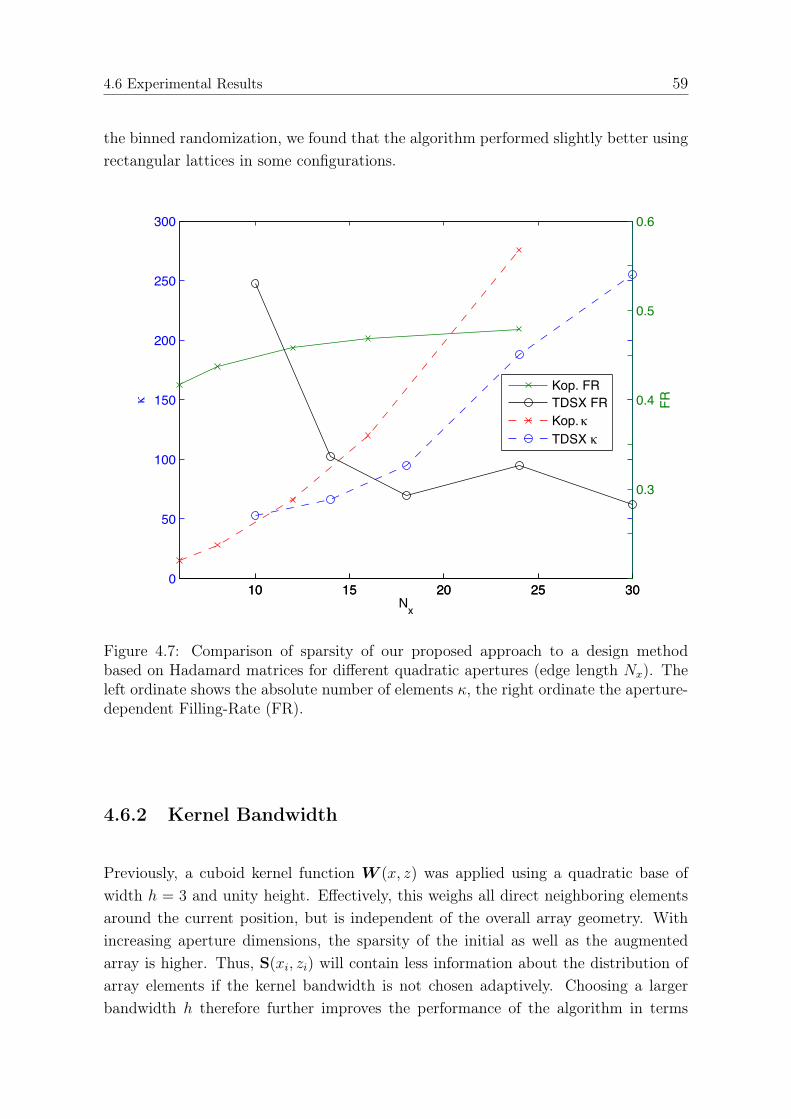
4.6 Experimental Results 59
the binned randomization, we found that the algorithm performed slightly better usingrectangular lattices in some configurations.
10 15 20 25 300
50
100
150
200
250
300
Nx
!
10 15 20 25 30
0.3
0.4
0.5
0.6
FR
Kop. FRTDSX FRKop. !TDSX !
Figure 4.7: Comparison of sparsity of our proposed approach to a design methodbased on Hadamard matrices for different quadratic apertures (edge length Nx). Theleft ordinate shows the absolute number of elements κ, the right ordinate the aperture-dependent Filling-Rate (FR).
4.6.2 Kernel Bandwidth
Previously, a cuboid kernel function W (x, z) was applied using a quadratic base ofwidth h = 3 and unity height. Effectively, this weighs all direct neighboring elementsaround the current position, but is independent of the overall array geometry. Withincreasing aperture dimensions, the sparsity of the initial as well as the augmentedarray is higher. Thus, S(xi, zi) will contain less information about the distribution ofarray elements if the kernel bandwidth is not chosen adaptively. Choosing a largerbandwidth h therefore further improves the performance of the algorithm in terms
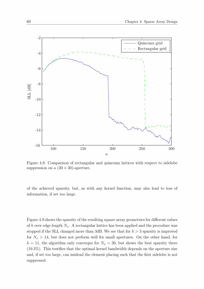
60 Chapter 4: Sparse Array Design
Figure 4.8: Comparison of rectangular and quincunx lattices with respect to sidelobesuppression on a (30× 30)-aperture.
of the achieved sparsity, but, as with any kernel function, may also lead to loss ofinformation, if set too large.
Figure 4.9 shows the sparsity of the resulting square array geometries for different valuesof h over edge length Nx. A rectangular lattice has been applied and the procedure wasstopped if the SLL changed more than 3dB. We see that for h > 3 sparsity is improvedfor Nx > 14, but does not perform well for small apertures. On the other hand, forh = 11, the algorithm only converges for Nx = 30, but shows the best sparsity there(19.3%). This testifies that the optimal kernel bandwidth depends on the aperture sizeand, if set too large, can mislead the element placing such that the first sidelobe is notsuppressed.
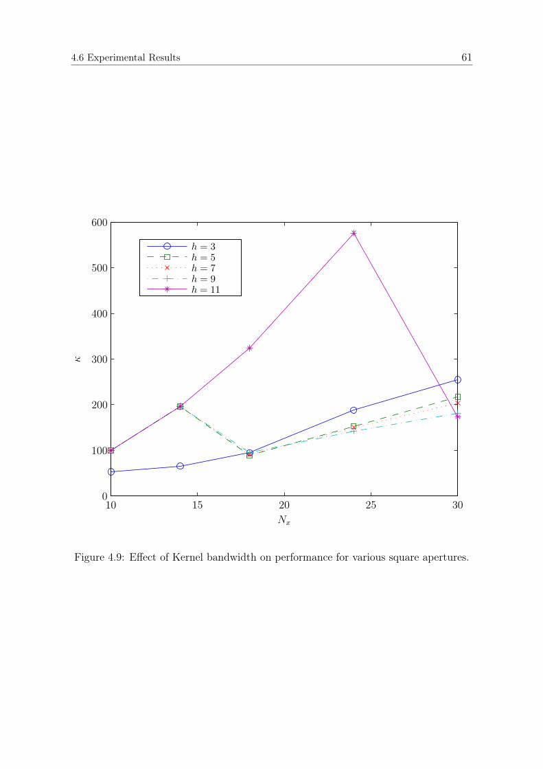
4.6 Experimental Results 61
Nx
κ
h = 3h = 5h = 7h = 9h = 11
10 15 20 25 300
100
200
300
400
500
600
Figure 4.9: Effect of Kernel bandwidth on performance for various square apertures.
62 Chapter 4: Sparse Array Design
4.6.3 Acoustic Imaging
Following the simulation results, we show here how an acoustic imaging system as de-scribed in Section 3.1 performs if it is based on sparse array layouts. The images in thissection are created by applying the array layouts obtained using the proposed methodsto select which data channels were selected from a full 18 × 18-array. The objectsare illuminated by a narrow-band excitation signal emitted around fc = 50 kHz, i.e.,λ ≈ 7 mm. The transmitter is specified to have a beam pattern such that the 3dB-cutoffarea is approximately 60◦ in azimuth and elevation. The reflected echoes are capturedby a receiving (18× 18)-array of acoustic, omnidirectional sensors (see also Section 3.1and [MZ07b]). The echoes scattered back from a large pole-object with a rough sur-face standing in front of the array. The different array layouts are tested by computingthe power pattern using only a subset of the full array’s sensors. We first comparethem based on their performance using Bartlett’s beamformer in order to illustratechanges that stem directly from the sparsity. However, since Bartlett beamformingsuffers generally from high sidelobes and results in speckle noise in acoustic imaging,the sparse array layouts are also evaluated using Capon’s adaptive beamformer, whichis the method that is actually used in the imaging system. Figure 4.10 shows thereceived power over azimuth angle φ and elevation angle θ for several array layoutsusing Bartlett’s beamformer. We compare an array with (16 × 16)-aperture with 120
elements based on Hadamard difference-sets according to [Kop08], a full (18x18)-URAwith 324 elements and an array with 95 elements according to the proposed techniquebased on a rectangular (18x18)-lattice.4 It can be seen that all three layouts result inimages where the contour of the pole object is visible. We also see how the regularsidelobe pattern of the beam-pattern of the URA results in regular artifacts in the im-age around the object (Figure 4.10 (b)). Both sparse layouts (Figure 4.10 (a) and (c))clearly show more severe and more irregular image artifacts due to the sparsity in thearrays. Additionally, the image in Figure 4.10 (c) shows higher sensitivity in end-firedirections. However, since the the imaging system is not operated in end-fire direction,the differences in those regions are not a matter of great interest. In Figure 4.11, weapplied Capon’s beamformer to the same layouts and data, meaning that the weightvector depends on the signal scenario and information from the covariance matrix es-timate is exploited, thus increasing the resolution and noise suppression in the images.Clearly, the image from the full array (Figure 4.11 (b)) shows the best contrast andalso the most uniform power reception from the object’s surface. In Figure 4.11 (a)and (c), it is shown that the sparsity leads to a slightly reduced contrast of the images.Additionally, both sparse layouts result in a less uniform power reception from the
4Unfortunately, we are not able to depict images using layouts based on randomization becausethe available array data stems from a uniform array.
4.6 Experimental Results 63
object, which could also be observed using Bartlett’s beamformer. The main differencebetween the two sparse array geometries is the altered reception of the object itself,an artifact that probably stems from the uneven sensor density across the aperture.Note that although the mainlobe of Bartlett’s beamformer is quasi-convex for this ar-ray geometry, this does not hold true for Capon’s beamformer because it calculatesthe weight vector adaptively. Additionally, the artifacts in end-fire directions are muchless visible than in the images obtained using H-set arrays. While this is beneficial ingeneral, the imaging system is not operated in end-fire direction anyway. Thus, thedifferences in those regions are not a matter of great interest. If the reception of powerfrom the object has to be improved, one can easily augment the array layout by theaddition of further elements. Their positions can then be obtained by starting thealgorithm initialized with the existing array.
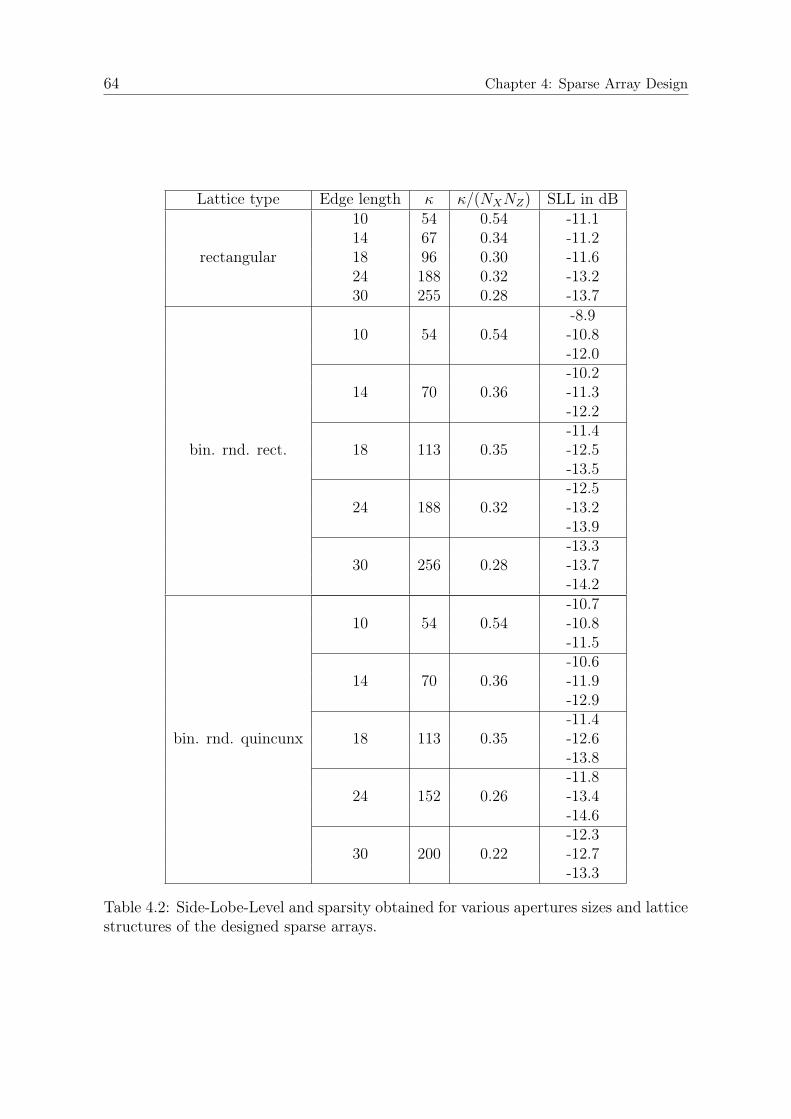
64 Chapter 4: Sparse Array Design
Lattice type Edge length κ κ/(NXNZ) SLL in dB10 54 0.54 -11.114 67 0.34 -11.2
rectangular 18 96 0.30 -11.624 188 0.32 -13.230 255 0.28 -13.7
-8.910 54 0.54 -10.8
-12.0-10.2
14 70 0.36 -11.3-12.2-11.4
bin. rnd. rect. 18 113 0.35 -12.5-13.5-12.5
24 188 0.32 -13.2-13.9-13.3
30 256 0.28 -13.7-14.2-10.7
10 54 0.54 -10.8-11.5-10.6
14 70 0.36 -11.9-12.9-11.4
bin. rnd. quincunx 18 113 0.35 -12.6-13.8-11.8
24 152 0.26 -13.4-14.6-12.3
30 200 0.22 -12.7-13.3
Table 4.2: Side-Lobe-Level and sparsity obtained for various apertures sizes and latticestructures of the designed sparse arrays.
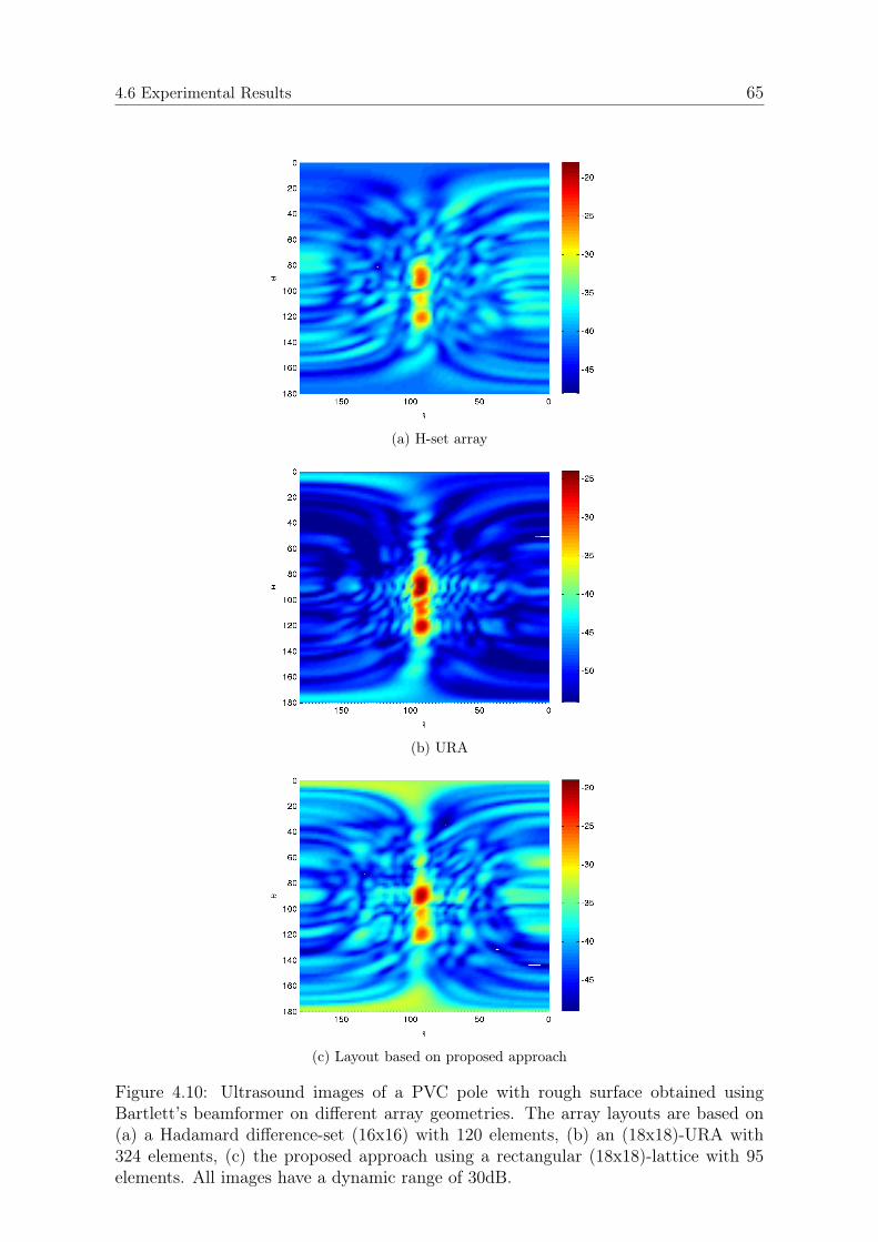
4.6 Experimental Results 65
(a) H-set array
(b) URA
(c) Layout based on proposed approach
Figure 4.10: Ultrasound images of a PVC pole with rough surface obtained usingBartlett’s beamformer on different array geometries. The array layouts are based on(a) a Hadamard difference-set (16x16) with 120 elements, (b) an (18x18)-URA with324 elements, (c) the proposed approach using a rectangular (18x18)-lattice with 95elements. All images have a dynamic range of 30dB.
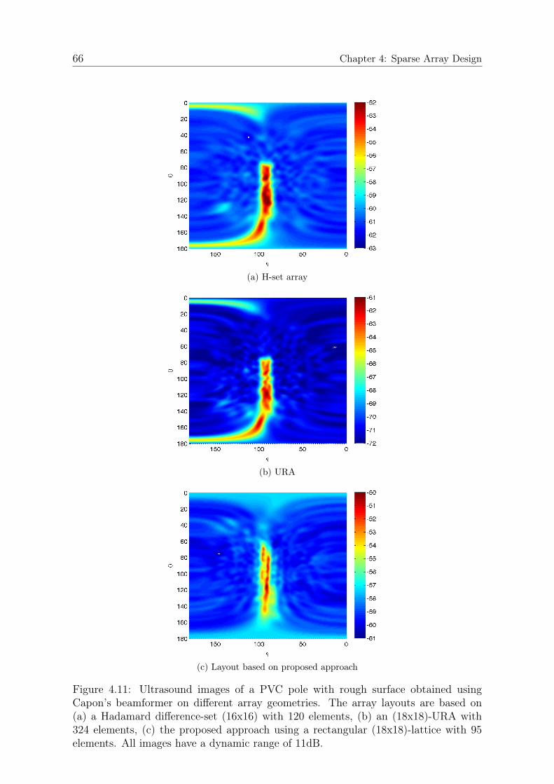
66 Chapter 4: Sparse Array Design
(a) H-set array
(b) URA
(c) Layout based on proposed approach
Figure 4.11: Ultrasound images of a PVC pole with rough surface obtained usingCapon’s beamformer on different array geometries. The array layouts are based on(a) a Hadamard difference-set (16x16) with 120 elements, (b) an (18x18)-URA with324 elements, (c) the proposed approach using a rectangular (18x18)-lattice with 95elements. All images have a dynamic range of 11dB.
67
Chapter 5
Human Detection and Classification
5.1 Introduction
While the previous chapters of this thesis address the problem of design and calibrationof an acoustic imaging systems, this chapter focuses on the question how such a systemcan be used in robotic applications. While it should be clear that objects can bedetected generally by the identification of peaks in the acoustic images, we will showthe possibility of detecting a class of objects which is of crucial importance for roboticapplications, namely the detection of humans. In robotics, for example, it is notonly generally important to detect obstacles in the surroundings of a system, butto specifically become aware of the presence of humans. Detecting persons in thesurroundings is crucial for control of robot awareness and navigation [LWLW06,BH09,STI08]. Based on the latter, the trajectory of a person can be estimated and the robotcan respond meaningfully, e.g., it can step out of the way of the human, address theperson, etc.
Before we go into more detail, we want to motivate the use of acoustic imaging in thiscontext. The benefits in this application will become even clearer after investigation ofthe limitations and weaknesses of other sensor modalities. In current systems, mainlyoptical (mono or stereo) cameras and radar are used [YTN05]. While it seems naturalto use optical sensors, these suffer from the fact that their performance varies greatlywith lighting conditions or employ expensive infrared cameras [LWLW06]. At the sametime, optical systems do not always reliably detect range and often assume motion ora specific shape of the persons [CD00,LWLW06]. To mitigate these limitations, theyoften employ complex multi-layered hierarchies inspired by biology (e.g., see [TBPI10]).Radar-based systems, on the other hand, are currently used, but require expensivehardware and can be unreliable due to the large variability and low intensity of radarreflections from humans [YTN05]. If we were interested in the detection of movingobjects only, using an acoustic or electro-magnetic excitation signal and the Dopplereffect would be sufficient. However, it would not be possible to detect all still standingobjects or persons in the scene.
Acoustic imaging allows for precise angular and range information. Due to the slowwave propagation speed of sound, we can easily discriminate close objects from back-ground and therefore identify obstacles in the surroundings. Additionally, we will show
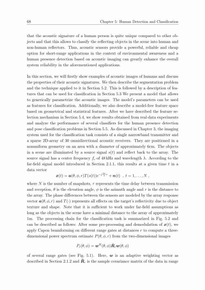
68 Chapter 5: Human Detection and Classification
that the acoustic signature of a human person is quite unique compared to other ob-jects and that this allows to classify the reflecting objects in the scene into human andnon-human reflectors. Thus, acoustic sensors provide a powerful, reliable and cheapoption for short-range applications in the context of environmental awareness and ahuman presence detection based on acoustic imaging can greatly enhance the overallsystem reliability in the aforementioned applications.
In this section, we will firstly show examples of acoustic images of humans and discussthe properties of their acoustic signatures. We then describe the segmentation problemand the technique applied to it in Section 5.2. This is followed by a description of fea-tures that can be used for classification in Section 5.3 We present a model that allowsto generically parametrize the acoustic images. The model’s parameters can be usedas features for classification. Additionally, we also describe a model-free feature spacebased on geometrical and statistical features. After we have described the feature se-lection mechanism in Section 5.4, we show results obtained from real-data experimentsand analyze the performance of several classifiers for the human presence detectionand pose classification problems in Section 5.5. As discussed in Chapter 3, the imagingsystem used for the classification task consists of a single narrowband transmitter anda sparse 2D-array of 30 omnidirectional acoustic receivers. They are positioned in anonuniform geometry on an area with a diameter of approximately 6cm. The objectsin a scene are illuminated by a source signal s(t) and reflect back to the array. Thesource signal has a center frequency fc of 48 kHz and wavelength λ. According to thefar-field signal model introduced in Section 2.1.1, this results at a given time t in adata vector
x(t) = a(θ, φ, r)T (s(t))e−j2πλτ + n(t) , t = 1, . . . , N ,
where N is the number of snapshots, τ represents the time delay between transmissionand reception, θ is the elevation angle, φ is the azimuth angle and r is the distance tothe array. The phase differences between the sensors are modeled by the array responsevector a(θ, φ, r) and T (·) represents all effects on the target’s reflectivity due to objecttexture and shape. Note that it is sufficient to work under far-field assumptions aslong as the objects in the scene have a minimal distance to the array of approximately1m. The processing chain for the classification task is summarized in Fig. 5.2 andcan be described as follows: After some pre-processing and demodulation of x(t), weapply Capon beamforming on different range gates at distances r to compute a three-dimensional power spectrum estimate P (θ, φ, r) from the two-dimensional images
Pr(θ, φ) = wH(θ, φ)Rrw(θ, φ)
of several range gates (see Fig. 5.1). Here, w is an adaptive weighting vector asdescribed in Section 2.1.2 and Rr is the sample covariance matrix of the data in range
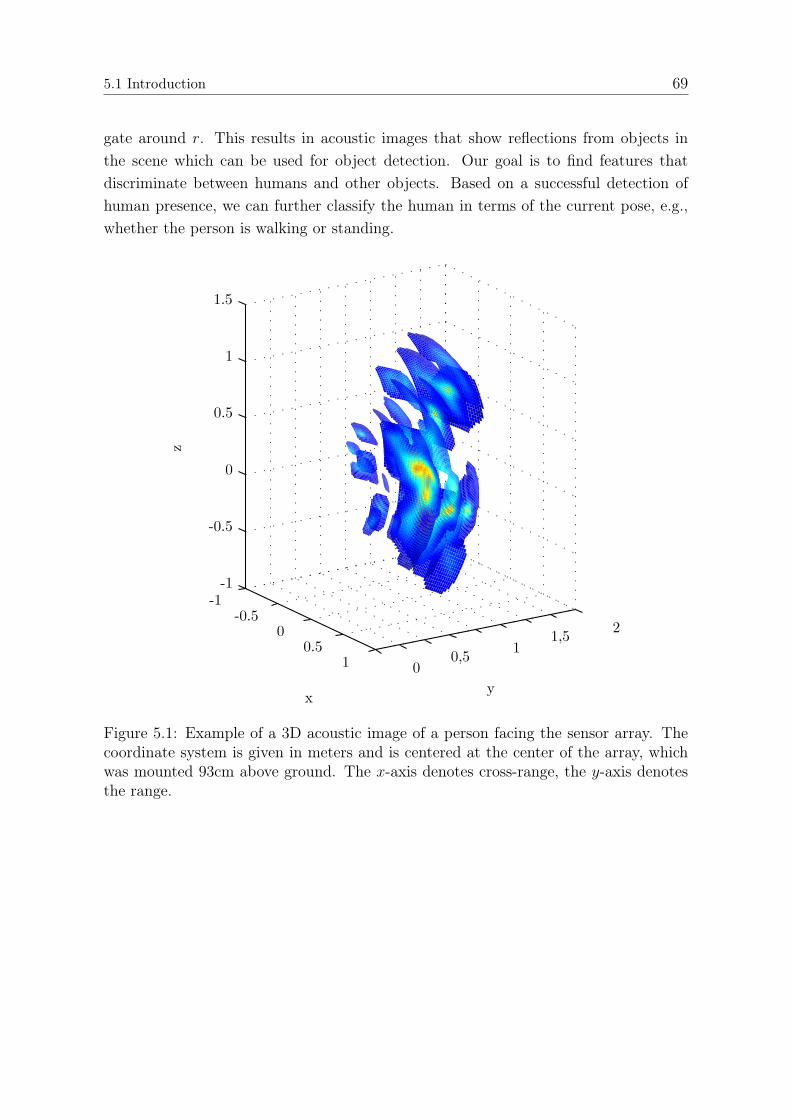
5.1 Introduction 69
gate around r. This results in acoustic images that show reflections from objects inthe scene which can be used for object detection. Our goal is to find features thatdiscriminate between humans and other objects. Based on a successful detection ofhuman presence, we can further classify the human in terms of the current pose, e.g.,whether the person is walking or standing.
Figure 5.1: Example of a 3D acoustic image of a person facing the sensor array. Thecoordinate system is given in meters and is centered at the center of the array, whichwas mounted 93cm above ground. The x-axis denotes cross-range, the y-axis denotesthe range.
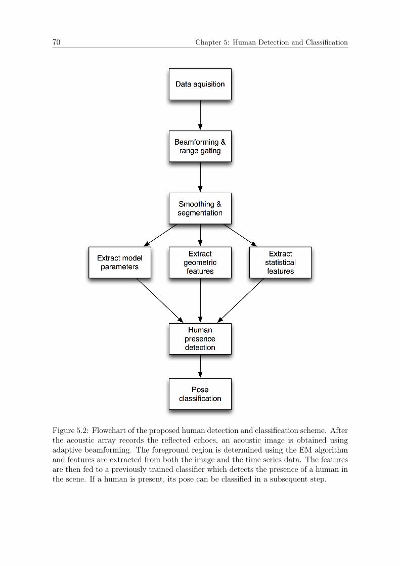
70 Chapter 5: Human Detection and Classification
Figure 5.2: Flowchart of the proposed human detection and classification scheme. Afterthe acoustic array records the reflected echoes, an acoustic image is obtained usingadaptive beamforming. The foreground region is determined using the EM algorithmand features are extracted from both the image and the time series data. The featuresare then fed to a previously trained classifier which detects the presence of a human inthe scene. If a human is present, its pose can be classified in a subsequent step.
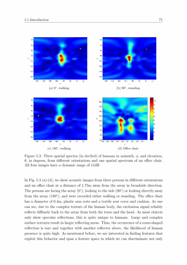
5.1 Introduction 71
(a) 0◦, walking (b) 90◦, standing
(c) 180◦, walking (d) Office chair
Figure 5.3: Three spatial spectra (in decibel) of humans in azimuth, φ, and elevation,θ, in degrees, from different orientations and one spatial spectrum of an office chair.All four images have a dynamic range of 11dB.
In Fig. 5.3 (a)-(d), we show acoustic images from three persons in different orientationsand an office chair at a distance of 1.75m away from the array in broadside direction.The persons are facing the array (0◦), looking to the side (90◦) or looking directly awayfrom the array (180◦), and were recorded either walking or standing. The office chairhas a diameter of 0.4m, plastic arm rests and a textile seat cover and cushion. As onecan see, due to the complex texture of the human body, the excitation signal reliablyreflects diffusely back to the array from both the torso and the head. As most objectsonly show specular reflections, this is quite unique to humans. Large and complexsurface textures result in larger reflecting areas. Thus, the occurrence of a torso-shapedreflection is rare and together with another reflector above, the likelihood of humanpresence is quite high. As mentioned before, we are interested in finding features thatexploit this behavior and span a feature space in which we can discriminate not only
72 Chapter 5: Human Detection and Classification
between humans and non-human objects, but also classify fundamental poses such asa walking movement in contrast to standing still.
5.2 Segmentation
To solve the classification problem formulated above, we need to segment the imagein order to detect the foreground region in a first step. This is followed by a featureextraction where the geometric features are based on properties of this foreground re-gion. Due to the nature of the excitation and reflection of sound, and the fact thatthe acoustic images are created by scanning the scene using beamforming, the imagewill not show any sharp edges, but rather smooth contours. The degree of smoothnessdepends mainly on the object’s shape and the beam-width of the applied beamformer,but is inevitable because the array has a limited aperture. Due to these facts, commoncomplex segmentation techniques traditionally used in the image processing commu-nity are not required here. For example, active contours [KWT88, BI98, CV01] ormin-cut/max-flow techniques [BK04, Set99] were mainly developed to segment highlydetailed images, e.g., photographic images or medical images from magnetic resonancebrain tomography [CJS93, FD96]. While such methods are undoubtedly very power-ful, they do not perform superior to simpler, threshold-based techniques when appliedto acoustic images, due to the relative simplicity of the shape of echoes. Thus, itis sufficient to detect acoustic echoes simply based on individual voxel power. Toachieve that, we smooth the image Pr(θ, φ) in an initial step to reduce potential multi-modalities of the torso echoes. We then use the EM algorithm [DLR77,RW84,Bis07] tofit a Gaussian-Mixture-Model (GMM) with two Gaussians G(µ1, σ1),G(µ2, σ2), whereµ1 < µ2, to the voxel intensity histogram of the smoothed image. Although the reflectedpower intensity can also be modeled according to a Rayleigh or Weibull distribution,a sufficient approximation can be obtained using a superposition of Gaussians, whichdirectly results in a low-intensity background and a high-intensity foreground region.The foreground region R is formed by voxels in the image that have a higher probabil-ity to belong to the Gaussian G(µ2, σ2) (see Fig. 5.4). This approach is well-known asa simple segmentation technique (e.g., see [Bis07]). In Figure 5.5, we show an exampleof the resulting foreground region where the head and torso echoes are not separatedinto distinct segments.
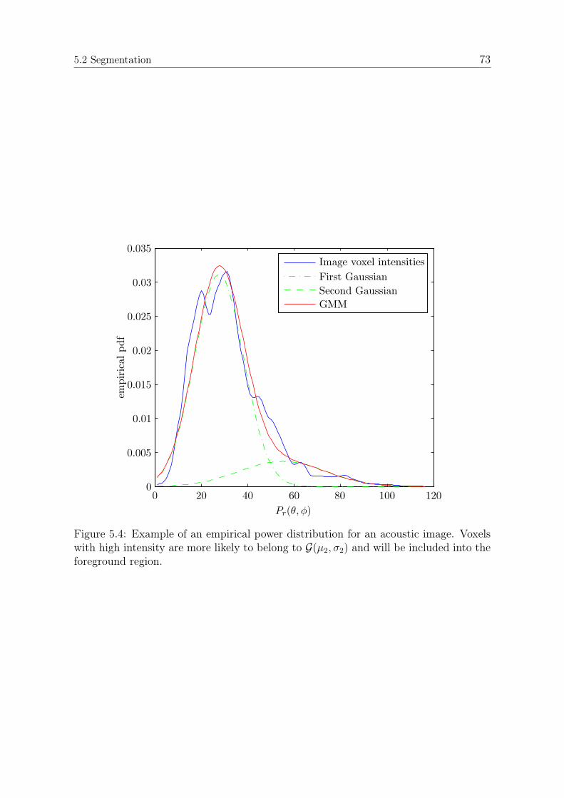
5.2 Segmentation 73
Figure 5.4: Example of an empirical power distribution for an acoustic image. Voxelswith high intensity are more likely to belong to G(µ2, σ2) and will be included into theforeground region.
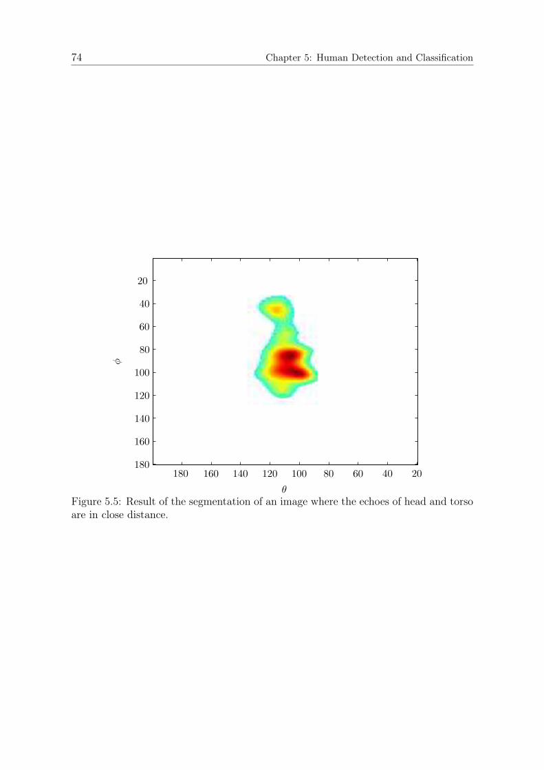
74 Chapter 5: Human Detection and Classification
Figure 5.5: Result of the segmentation of an image where the echoes of head and torsoare in close distance.

5.3 Feature Extraction 75
5.3 Feature Extraction
In order to obtain a feature space for human presence detection or classification of aspecific pose, we extract features from the acoustic images in three different ways:
1. First, we formulate a generic model for acoustic images and extract the model’sparameters as features.
2. Secondly, we extract statistical features from the time series data x(t) recordedby the array.
3. Finally, we also extract geometric features from the acoustic images Pr(θ, φ)
obtained from x(t).
In the following, we describe each of those ways in more detail. The implementedfeatures are chosen such that they correspond to some physical meaning or imageparameter that changes with respect to the object in the scene, e.g., the contours of themain echoes or the size of its reflective surface. While it is easily possible to implementmany more shape parameters, we restrict the presentation to the features that are usedin the classification. Their choice is motivated not only by physical meaning, but alsoan information-theoretic feature selection procedure described in Section 5.4. This isalso validated by the achieved classification performance we describe in Section 5.5.The features are described such that their values are affected by the object’s range.However, it is straightforward to make them range-invariant by transforming them tothe Cartesian coordinate system and/or normalize them with respect to their TOF.
5.3.1 Modeling the Acoustic Signature
In this section, we describe how the acoustic images can be generically modeled. Ourgoal is to extract the model parameters as features for further classification of theobjects present in the scene. We are interested in two aspects, based on the reliableoccurrence of head and torso echoes. First, we want to parametrize the image suchthat the acoustic signature is preserved and we can establish geometric propertiesin the image. Secondly, we aim to find clusters in the parameter space that allowus to discriminate between humans and other objects present in the scene. Withrespect to the detection and classification of persons, this means that we want toobtain parameter sets that are unique to the presence of a large torso echo, a weaker
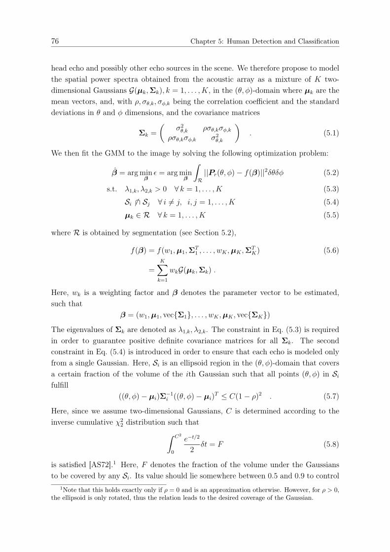
76 Chapter 5: Human Detection and Classification
head echo and possibly other echo sources in the scene. We therefore propose to modelthe spatial power spectra obtained from the acoustic array as a mixture of K two-dimensional Gaussians G(µk,Σk), k = 1, . . . , K, in the (θ, φ)-domain where µk are themean vectors, and, with ρ, σθ,k, σφ,k being the correlation coefficient and the standarddeviations in θ and φ dimensions, and the covariance matrices
Σk =
(σ2θ,k ρσθ,kσφ,k
ρσθ,kσφ,k σ2θ,k
). (5.1)
We then fit the GMM to the image by solving the following optimization problem:
β = arg minβε = arg min
β
∫R||Pr(θ, φ)− f(β)||2δθδφ (5.2)
s.t. λ1,k, λ2,k > 0 ∀ k = 1, . . . , K (5.3)
Si 6 ∩ Sj ∀ i 6= j, i, j = 1, . . . , K (5.4)
µk ∈ R ∀ k = 1, . . . , K (5.5)
where R is obtained by segmentation (see Section 5.2),
f(β) = f(w1,µ1,ΣT1 , . . . , wK ,µK ,Σ
TK) (5.6)
=K∑k=1
wkG(µk,Σk) .
Here, wk is a weighting factor and β denotes the parameter vector to be estimated,such that
β = (w1,µ1, vec{Σ1}, . . . , wK ,µK , vec{ΣK})
The eigenvalues of Σk are denoted as λ1,k, λ2,k. The constraint in Eq. (5.3) is requiredin order to guarantee positive definite covariance matrices for all Σk. The secondconstraint in Eq. (5.4) is introduced in order to ensure that each echo is modeled onlyfrom a single Gaussian. Here, Si is an ellipsoid region in the (θ, φ)-domain that coversa certain fraction of the volume of the ith Gaussian such that all points (θ, φ) in Sifulfill
((θ, φ)− µi)Σ−1i ((θ, φ)− µi)T ≤ C(1− ρ)2 . (5.7)
Here, since we assume two-dimensional Gaussians, C is determined according to theinverse cumulative χ2
2 distribution such that∫ C2
0
e−t/2
2δt = F (5.8)
is satisfied [AS72].1 Here, F denotes the fraction of the volume under the Gaussiansto be covered by any Si. Its value should lie somewhere between 0.5 and 0.9 to control
1Note that this holds exactly only if ρ = 0 and is an approximation otherwise. However, for ρ > 0,the ellipsoid is only rotated, thus the relation leads to the desired coverage of the Gaussian.

5.3 Feature Extraction 77
the separation between the Gaussians effectively. The third constraint in Eq. (5.5) isbased on the segmentation result and simply restricts the mean of the Gaussians tolie inside the foreground region. It is not strictly necessary, but prevents divergence ofthe solving algorithm from reasonable solutions. The problem formulated in Eq. (5.2)can be initialized using knowledge of R, e.g. the mean vectors µk, k = 1, . . . , K can bedefined to be at the locations of the K largest extrema in R.
To accelerate the convergence properties in the solution space, it is beneficial to refor-mulate the constraints in Eq. (5.3) and (5.5) into penalty terms of the cost function,e.g. a positive definite Σk can be favored by a penalty term log(det Σk). The constraintin Eq. (5.5) can be taken into account by penalizing the distance of µk to the centerof mass of R. Thus, the problem from Eq. (5.2) can be reformulated to
β = arg minβε = arg min
β
∫R||Pr(θ, φ)− f(β)||2δθδφ (5.9)
− l1 log(det Σk) + l2∑k
log(det Σk)||µk − (θ, φ)||
s.t. Si 6 ∩ Sj ∀ i 6= j (5.10)
Here, l1, l2 represent constant penalty cost factors that have to be chosen manuallyand control the weighting of the different terms in the cost function. The point (θ, φ)
denotes the center of gravity in the foreground region R and is defined by
θ =
s
RθPr(θ, φ)δθδφ
s
RPr(θ, φ)δθδφ
, φ =
s
RφPr(θ, φ)δθδφ
s
RPr(θ, φ)δθδφ
(5.11)
The problem in Eq. (5.9) can be solved numerically, e.g. using a Quasi-Newton algo-rithm, for different K, depending on the target object class, i.e.. As the knees, handsand feet of humans are not always visible in the image, it is sufficient to set K = 2
to model only the head and torso echoes, assuming there are not other objects presentin the scene. Clearly, one has to set K higher when there is no knowledge about thescene and the number of reflectors available.
Based on the found estimate of the model parameters β, we can then formulate otherfeatures that are meaningful to detect humans in the image, e.g. the relative position,distance and angle of the centroids. Additionally, we can expect the head echo to bemuch smaller than the torso echo, meaning that the ratio of variances is an additionalfeature. However, the solution of Eq. (5.9) provides not only β, but also the residu-als ε as a measure for the goodness-of-fit of the model. Therefore, it is theoreticallypossible to set K as a free parameter and vary the model order. One can then choosehow accurately the image should be modeled or whether small reflectors, clutter and
78 Chapter 5: Human Detection and Classification
noise should also be modeled or neglected. The classic information criteria can thenbe used to balance model accuracy versus complexity based on the principle of par-simony (see [SS04,WK85,WZ89]). Together with the segmentation contours, β andε allow to represent humans in acoustic images quite uniquely and can be suppliedto a subsequent classifier. A strong advantage of the method is that head and torsoechoes of a human are always explicitly determined, such that it works reliably evenwhen those echo regions are so close that the segmentation does not find disjoint re-gions anymore. On the other hand, the approach has the sever disadvantage that theformulated optimization problem is based on the least-squares principle and requirescomplex problem solving routines. The accuracy of the resulting model also dependsheavily on the initialization of the problem. We therefore seek to also find more simplefeatures that are easy to compute and do not rely on complex optimization problems
5.3.2 Geometric Features
5.3.2.1 Elliptic Torso Fitting
For the above mentioned reasons, the use of ellipse fitting is a reasonable choice, since itis computationally cheap. Additionally, the torso is not only a reliable source of acousticreflection of any human, but also shows a significant elliptic shape. We therefore modelthe contours of the largest echoes in the foreground region R. We assume that thesegment with the largest area represents the torso and extract its contourC = (cθ cφ)T ,where cθ, cφ represent the coordinates of the contour pixels and are, thus, of varyinglength and the superscript T denotes transpose. Now, given the general quadraticexpression of an ellipse as
CTe Σ−1Ce + c = 0 , (5.12)
we can transform the data by subtraction of its center of mass and rotation to obtaina standardized ellipse of the form
CTe SCe + c = 0 .
With λ1, λ2 being the eigenvalues of Σ−1, a =√− cλ1, b =
√− cλ2
are the ellipse’saxes and, since λ1, λ2 are invariant to translation and rotation, S = diag(λ1, λ2). Wethen fit the ellipse parameters to the data by minimizing the geometric distances ofthe ellipse to C, meaning that we minimize the sum of the squares of the distancesto the data points [GGS94]. This can be obtained using the constraint λ1 + λ2 = 1
(or trace(S) = 1). This has been shown to be more robust than minimizing thealgebraic distances [GGS94,FPF99,FF95] and results in a nonlinear (total) least squares
5.3 Feature Extraction 79
problem which we solve using a Gauss-Newton procedure following [GGS94]. The initialestimates of the parameters are found using the Bookstein constraint λ2
1+λ22 = 1, which
is more efficient, but not as accurate as the trace constraint. In [FPF99], an alternativeapproach is given and the authors show that their strategy is even more robust for thegeneral problem of conic fitting. However, we found that for the acoustic images, usingthe trace constraint as described above is sufficient and the results do not differ largely.
5.3.2.2 Generic Shape Parameters
In addition to the elliptic parameters, we also use more generic shape parameters of theacoustic images. The most simple feature used here is the total area A of the largestcontinuous segment in R. Based on that, we also compute a measure of smoothness ofthe contours. We implemented several features such as the model order of a polygonalfit to the contour, the eccentricity of the contour in polar coordinates and also moresophisticated transformations of the contour (see also [ZL04]). However, we found thata rather simple measure performed best from this category of features. To obtain it,we determine the smallest convex polygon that fully contains the echo segment anddetermine its area Ac. Then, simply the convexity
cv = Ac/A
shows how smooth the contour of an echo segment is. The feature selection describedin Section 5.4 showed that this convexity dominates other shape parameters than A
for the problem of pose classification.
5.3.3 Statistical Features
In addition to features extracted from the acoustic images, we also analyze the timeseries data of the array channels in x(t). They contain direct information about echodistribution in depth as well as information about the object’s general pose. An analysisof the distribution of the data shows changes within the classes. More specifically,the extreme values as well as the percentile spreads in the empirical distributions arecorrelated with the reflecting surface of the objects in the scene, suggesting that thetails of the distributions change depending on the human pose. This is likely due to thefact that a walking human rotates the body slightly. The received power will thereforevary in signal strength because the reflections stem from reflective surfaces that arenot orthogonal to the direct line between array and person. For these reasons, weextract features which estimate the tails of the time series as well as measures of powerconcentration along the range.
80 Chapter 5: Human Detection and Classification
5.3.3.1 Hill Estimator
There exist several indices that measure the extent to which a distribution is heavy-tailed (see [PDM98] for an overview). Here, we use the Hill estimator [Hil75] which isdefined as follows: Let X(1), X(2), . . . , X(n) be the order statistics, obtained by X(1) ≥X(2) ≥ . . . ≥ X(n), of a distribution F (x) and x(1) ≥ x(2) ≥ . . . ≥ x(N) realizationsthereof. F (x) can be of any form, but its (upper) tail should follow a general formsuch that for large x, 1 − F (x) ∝ x−α. A value of α = 1 corresponds to the Cauchydistribution and distributions with α→ 2 approach the normal distribution [PDM98].The Hill estimator of the tail index of F (x) is then given by
α(m)H =
m+ 1∑mi=1 i · ln
(x(i)
x(i+1)
) ,
where m is the number of order statistics taken into account in the estimation. Thechoice of m influences the statistical properties of α(m)
H , e.g., a large m will result ina small variance, but a large bias of the estimator. An iterative selection procedureto choose m optimally is described in [Hsi99]. Applied to this problem, it results inapproximately m = 0.2N . Clearly, the samples x(n) could be taken from any singlechannel of the array. At the same time, it is advisable to make use of all the data in x(t),not only a single channel. However, one should not simply merge data from differentchannels in order to increase the sample size as the channels are highly correlatedand the Hill estimator was developed based on the assumption of independent andidentically distributed statistics. Alternatively, we average the absolute values of thedata across all channels in the base-band to obtain a pseudo-channel x(t), t = 1, . . . , N
with order statistics X(i), which greatly reduces the variance of α(m)H compared to using
a single channel.
5.3.3.2 Power-related Tail Parameters
Since α(m)H is a shape parameter that does not contain information about the strength of
the received echoes, we additionally look at other measures based on the samples abovethe 80-percentile of the empirical distribution, denoted by x(i)
0.8 = x(m), . . . , x(1) ,m =
b0.2Nc to obtain more information about the maximally returned power. We thenestimate both the sample mean and the sample variance in the upper tail as
µ0.8 =1
m
m∑i=1
x(i)
5.4 Feature Selection 81
and
σ0.8 =1
m− 1
m∑i=1
(x(i) − µ0.8)2 .
These features measure the amount of power and the concentration in the tail, whichconsistently shows to possess discriminative power especially for the pose classification(see Section 5.5.4).
5.3.3.3 Depth-related Parameters
As the reflected echoes from the objects vary across range depending on the shape ofan object or the pose of a human, it is reasonable to also measure the concentrationof power along the distance to the array. While walking humans will most likely swingtheir arms during movement, a standing human is expected to hold them closer totheir bodies most of the time. This results in the fact that walking humans on averagereflect echoes across a larger range than standing humans. To measure this effect,we estimate central geometric moments in the pseudo-channel, i.e., the moment offirst order by m1 =
∑Ni=1 x(i)(i − tp)2, where tp denotes the location of the point of
mass along the samples. If a human is present, tp will correspond to the depth atwhich the torso reflects the largest echo. To obtain an even stronger emphasis on thepower received, we also estimate the second central geometric moment, which is simplym2 =
∑Ni=1 x
2(i)(i− tp)2.
5.4 Feature Selection
To select a good feature subset for the human presence detection, it is reasonable toselect features that are heavily affected by the presence of a large torso echo from thehuman. Thus, we manually choose to select the ellipse’s axis parameters a, b obtainedfrom the elliptic fit of the largest echo. Together with the reflective area A, we obtaina three-dimensional feature space that is well separated (see Section 5.5.3). However,the selection of features is more complex for the problem of pose classification. While itis straightforward to identify several features that are clearly correlated with the classlabel, the selection of a reasonable feature subspace for that problem is more difficultand a statistical analysis of the feature space is necessary to obtain good classificationperformance.
There exist numerous approaches for feature selection such as sequential searches, ge-netic algorithms, branch-and-bound search (see [JZ97] for an overview). They all have
82 Chapter 5: Human Detection and Classification
in common that they need to define a measure of merit in order to evaluate a specificfeature space for some training data. The most common measure here is the clas-sification error rate, which determines how accurate a specific classifier performs inseparating data into a number of classes. However, it can only be calculated by choos-ing a certain classifier which has to be retrained for every feature subset. While this isclearly possible, there is also the possibility to analyze the feature space and possiblesubspaces without the need of a specific classifiers. We use the minimal-Redundancy-Maximal-Relevance (mRMR) method of [PLD05], which is proven to give results thatmaximize the dependency of the class labels on the selected features. The methodrelies on the mutual information between two random variables X and Y , defined as
I(X, Y ) =x
p(x, y) logp(x, y)
p(x)p(y)dxdy .
The relevance of a set S of features is then measured by the averaged mutual informa-tion of all features with the class labels as
D(S, Cn) =1
|S|∑fi∈S
I(fi, Cn)
and the redundancy of S is measured by the average mutual information between twofeatures fi, fj as
R(S) =1
|S|2∑
fi,fj∈S
I(fi, fj) .
The algorithm maximizes the relevance while simultaneously minimizing the redun-dancy in S. This is performed by maximizing the difference D(S, Cn) − R(S) withrespect to single features in S. Thus, a set with high discriminative power is createdusing only a small number of features that complement one another. Kernel densityestimation is used to obtain estimates of D and R. Gaussian kernels have been foundto be suitable. The features are then selected using an incremental search that addsone feature at a time. In [PLD05], this "first-order incremental selection” is shown tobe optimal in that it maximizes the dependency of the class label on the resulting fea-ture subspace. The features selected with this procedure are the ones described in theprevious section. They also validate the manual selection of the elliptical parametersand the torso area as sufficient for the human detection problem because additionalfeatures only have a small effect on D(S, Cn) while increasing R(S). While it is suffi-cient to use only geometric features for the detection problem, only the combinationof features from statistical and geometric categories allows a reasonable classificationperformance for the pose classification problem. The GMM parameters can be used fora successful detection, but are inferior to the simpler geometric features described insection 5.3.2 due to their complexity. We therefore show the results using the model-based approach, but do not further include those parameters in the feature space forthe classification results.
5.5 Results 83
5.5 Results
In this section, we present the experimental setup used to record the real data on whichthe results in this section are based. We will compare the classification performanceof several methods for both the human presence detection and the pose classificationproblem. All features are scaled before any feature selection, training or testing toavoid numerical dominance of any feature. The scaling factors were chosen such thatall features lie in the interval from 0 to 1. We apply four different classifiers to allclassification problems:
• a simple LDA classifier that assumes homoscedastic (equal covariance matrices)distributions for the classes,
• a QDA classifier that makes no assumptions about the covariances of the classes,
• SVMs using a linear kernel,
• and SVMs using a Gaussian radial basis function as kernel.
The performance is compared based on the same training and test data. The SVMswere tested with several penalty terms and function parameters (e.g. variances ofthe Gaussian kernels). The described results are obtained using the best choice ofparameters from a logarithmic grid search.
5.5.1 Experimental Setup
The imaging system we use consists of a single narrow-band acoustic transmitter witha center-frequency of 48 kHz. The receiving 2D-array consists of 30 omnidirectionalmicrophones which are positioned in a nonuniform sparse geometry. It is mounted ata height of 93cm. The transmitter is specified to have a beam pattern such that the3dB-cutoff area is approximately 60◦ in azimuth and elevation and is mounted close tothe array. The system was placed in an indoor scenario and we recorded several datasets from humans and non-human objects. The class of non-human objects consists ofseveral pieces of typical office furniture, such as an office chair, a desk, a room plant,etc. All objects were put in front of the array at different orientations relative to thearray and the scene was illuminated by the single transmitter. The recorded echos werethen processed using adaptive beamforming as described in Sections 2.1.2 and 3.1.
84 Chapter 5: Human Detection and Classification
5.5.2 Modeling Results
We demonstrate the approach described above and apply it to data from two differentscenes, each containing a single object. In the first scene, a human was standing infront of the array at a distance of 1.75m, facing the array. In the second scene, theoffice chair from Figure 5.3 was placed at the same position. In Figure 5.6, we cansee the reconstructed images based on the segmentation region R and the estimatedparameters β for a GMM withK = 2. The resulting image for the first scene (Fig. 5.6a)clearly shows the Gaussian that models the strong torso echo (w1 = 8.296) while thehead echo, modeled by a significantly weaker Gaussian above (w2 = 3.637), is lessstrongly visible, but reliably located above the torso as expected. Thus, although thetwo echo sources were not well separated, the image was successfully parametrized.In the second scene, the two strongest echoes are reflected from both one of the armrests and a corner of the seat cushion. This is also modeled in the reconstructed image(Fig. 5.6b), where only two smaller, almost equally strong reflections are modeled atboth corresponding regions in the image. We see that modeling the acoustic imageby a GMM allows to represent the spatial information about the position of reflectingsurfaces in a parameter vector. As described previously, the approach can be extendedby application of the model with a varying order K if it is desired to model the imagein more detail, resulting in a model-order selection problem.
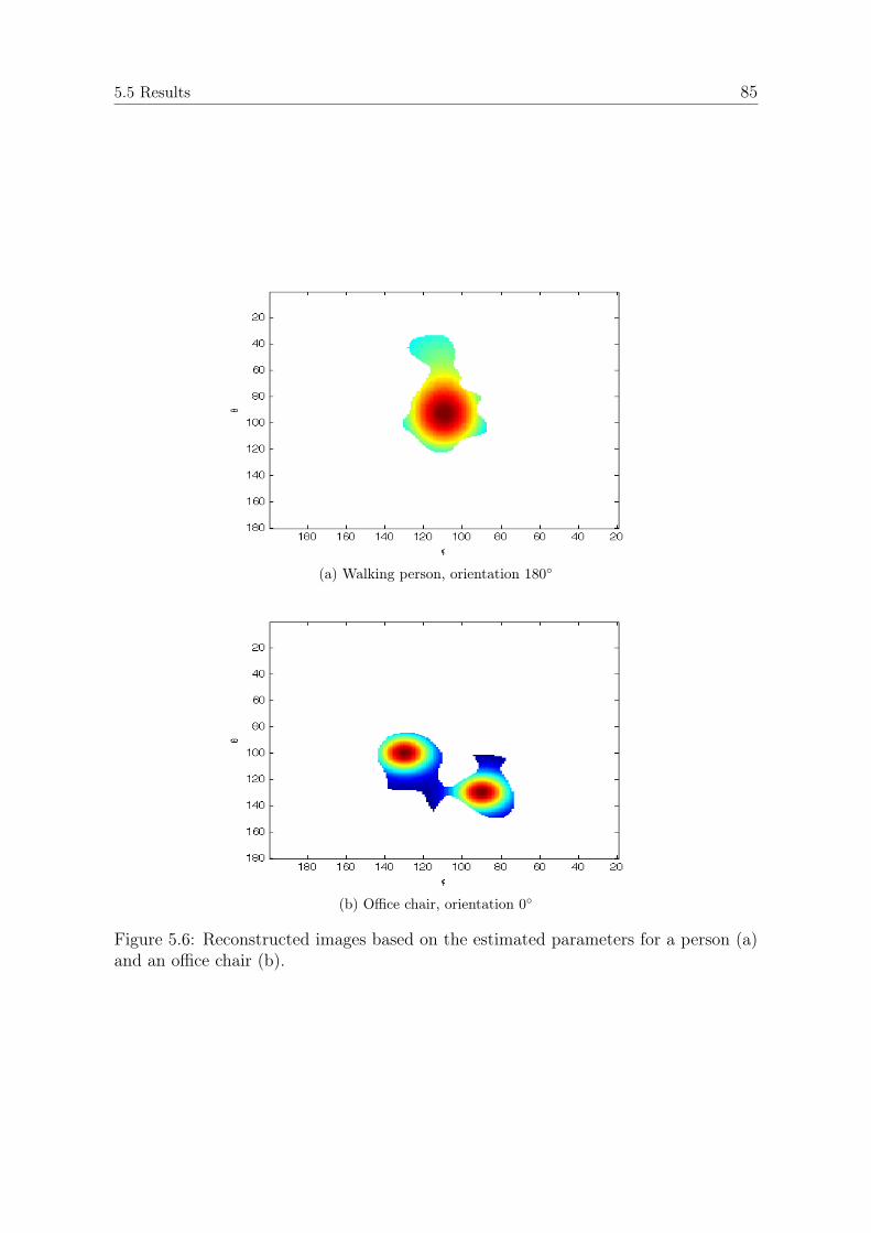
5.5 Results 85
(a) Walking person, orientation 180◦
(b) Office chair, orientation 0◦
Figure 5.6: Reconstructed images based on the estimated parameters for a person (a)and an office chair (b).
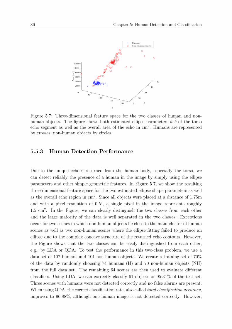
86 Chapter 5: Human Detection and Classification
Figure 5.7: Three-dimensional feature space for the two classes of human and non-human objects. The figure shows both estimated ellipse parameters a, b of the torsoecho segment as well as the overall area of the echo in cm2. Humans are representedby crosses, non-human objects by circles.
5.5.3 Human Detection Performance
Due to the unique echoes returned from the human body, especially the torso, wecan detect reliably the presence of a human in the image by simply using the ellipseparameters and other simple geometric features. In Figure 5.7, we show the resultingthree-dimensional feature space for the two estimated ellipse shape parameters as wellas the overall echo region in cm2. Since all objects were placed at a distance of 1.75m
and with a pixel resolution of 0.5◦, a single pixel in the image represents roughly1.5 cm2. In the Figure, we can clearly distinguish the two classes from each otherand the large majority of the data is well separated in the two classes. Exceptionsoccur for two scenes in which non-human objects lie close to the main cluster of humanscenes as well as two non-human scenes where the ellipse fitting failed to produce anellipse due to the complex concave structure of the returned echo contours. However,the Figure shows that the two classes can be easily distinguished from each other,e.g., by LDA or QDA. To test the performance in this two-class problem, we use adata set of 107 humans and 101 non-human objects. We create a training set of 70%
of the data by randomly choosing 74 humans (H) and 70 non-human objects (NH)from the full data set. The remaining 64 scenes are then used to evaluate differentclassifiers. Using LDA, we can correctly classify 61 objects or 95.31% of the test set.Three scenes with humans were not detected correctly and no false alarms are present.When using QDA, the correct classification rate, also called total classification accuracy,improves to 96.88%, although one human image is not detected correctly. However,
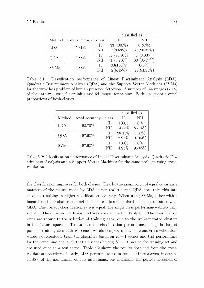
5.5 Results 87
classified asMethod total accuracy class H NH
LDA 95.31%H 33 (100%) 0 (0%)NH 3(9.68%) 28(90.32%)
QDA 96.88%H 32 (96.97%) 1 (3.03%)NH 1 (3.23%) 30 (96.77%)
SVMs 96.88%H 33(100%) 0(0%)NH 2(6.45%) 29(93.55%)
Table 5.1: Classification performance of Linear Discriminant Analysis (LDA),Quadratic Discriminant Analysis (QDA) and the Support Vector Machines (SVMs)for the two-class problem of human presence detection. A number of 144 images (70%)of the data was used for training and 64 images for testing. Both sets contain equalproportions of both classes.
classified asMethod total accuracy class H NH
LDA 92.79%H 100% 0%NH 14.85% 85.15%
QDA 97.60%H 98.13% 1.87%NH 2.97% 97.03%
SVMs 97.60%H 100% 0%NH 4.95% 95.05%
Table 5.2: Classification performance of Linear Discriminant Analysis, Quadratic Dis-criminant Analysis and a Support Vector Machines for the same problem using cross-validation.
the classification improves for both classes. Clearly, the assumption of equal covariancematrices of the classes made by LDA is not realistic and QDA does take this intoaccount, resulting in higher classification accuracy. When using SVMs, either with alinear kernel or radial basis functions, the results are similar to the ones obtained withQDA. The correct classification rate is equal, the single class performance differs onlyslightly. The obtained confusion matrices are depicted in Table 5.1. The classificationrates are robust to the selection of training data, due to the well-separated clustersin the feature space. To evaluate the classification performance using the largestpossible training sets with K scenes, we also employ a leave-one-out cross-validation,where we repeatedly train the classifiers based on K − 1 scenes and test performancefor the remaining one, such that all scenes belong K − 1 times to the training set andare used once as a test scene. Table 5.2 shows the results obtained from the cross-validation procedure. Clearly, LDA performs worse in terms of false alarms, it detects14.85% of the non-human objects as humans, but maintains the perfect detection of

88 Chapter 5: Human Detection and Classification
all humans. In summary, LDA results in a classifier that is biased towards humans. Itis not generally recommendable due to its simple linear decision rule and assumptionsabout the equal covariance of the classes. Both QDA and SVMs perform better intotal classification accuracy. However, the results using SVMs indicate also a biastowards humans, although on a much smaller scale. The quadratic classifier shows amore balanced result, at the cost of a slightly reduced detection of humans. Its totalclassification accuracy is again identical to the one obtained using SVMs.
5.5.4 Pose Classification Performance
To analyze the classification performance for standing and walking humans, we recordedanother data set of 73 scenes in which one of 4 different persons is present at a time.The subjects were recorded both while walking and standing and looking at differentdirections relative to the array (0◦, 90◦, 180◦, 270◦). The persons were recorded duringsix poses while walking a full sequence of steps which forms the basis of a periodicwalking movement. In the following, we describe the recorded poses with an exampleof a walking movement that starts with the right leg:
1. Initially, the person stands on one foot (e.g. the left) and extends the other tostep forward.
2. In the second pose, the person has shifted weight to the other (right) foot andstands on it while the heel of the initial (left) foot is lifted from the ground.
3. The next sample is recorded when the person’s initial (left) foot is moved forwardand is parallel to the standing foot. Weight is still on the other (right) foot. Theknee of the left foot is slightly bent, the foot above ground.
4. Afterwards, the person extends the left leg forward, placing the heel on theground, while body weight is still mainly on the right foot.
5. Again, body weight is shifted during the step such that the person lifts the heelof the right foot and is now standing on the left foot.
6. In the last pose of the sequence, the person pulls the right leg forward. Therecorded pose is symmetric to pose 3.
A walking person will periodically follow this sequence of poses. Due to the similarityof pose 3 and 6 to a standing pose, it is hard to decide binary between a walking and
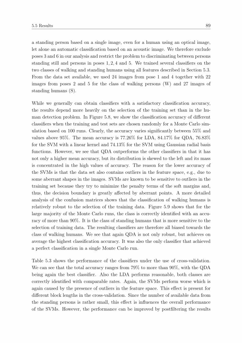
5.5 Results 89
a standing person based on a single image, even for a human using an optical image,let alone an automatic classification based on an acoustic image. We therefore excludeposes 3 and 6 in our analysis and restrict the problem to discriminating between personsstanding still and persons in poses 1, 2, 4 and 5. We trained several classifiers on thetwo classes of walking and standing humans using all features described in Section 5.3.From the data set available, we used 24 images from pose 1 and 4 together with 22images from poses 2 and 5 for the class of walking persons (W) and 27 images ofstanding humans (S).
While we generally can obtain classifiers with a satisfactory classification accuracy,the results depend more heavily on the selection of the training set than in the hu-man detection problem. In Figure 5.8, we show the classification accuracy of differentclassifiers when the training and test sets are chosen randomly for a Monte Carlo sim-ulation based on 100 runs. Clearly, the accuracy varies significantly between 55% andvalues above 95%. The mean accuracy is 77.26% for LDA, 84.17% for QDA, 76.83%
for the SVM with a linear kernel and 74.13% for the SVM using Gaussian radial basisfunctions. However, we see that QDA outperforms the other classifiers in that it hasnot only a higher mean accuracy, but its distribution is skewed to the left and its massis concentrated in the high values of accuracy. The reason for the lower accuracy ofthe SVMs is that the data set also contains outliers in the feature space, e.g., due tosome aberrant shapes in the images. SVMs are known to be sensitive to outliers in thetraining set because they try to minimize the penalty terms of the soft margins and,thus, the decision boundary is greatly affected by aberrant points. A more detailedanalysis of the confusion matrices shows that the classification of walking humans isrelatively robust to the selection of the training data. Figure 5.9 shows that for thelarge majority of the Monte Carlo runs, the class is correctly identified with an accu-racy of more than 90%. It is the class of standing humans that is more sensitive to theselection of training data. The resulting classifiers are therefore all biased towards theclass of walking humans. We see that again QDA is not only robust, but achieves onaverage the highest classification accuracy. It was also the only classifier that achieveda perfect classification in a single Monte Carlo run.
Table 5.3 shows the performance of the classifiers under the use of cross-validation.We can see that the total accuracy ranges from 79% to more than 90%, with the QDAbeing again the best classifier. Also the LDA performs reasonable, both classes arecorrectly identified with comparable rates. Again, the SVMs perform worse which isagain caused by the presence of outliers in the feature space. This effect is present fordifferent block lengths in the cross-validation. Since the number of available data fromthe standing persons is rather small, this effect is influences the overall performanceof the SVMs. However, the performance can be improved by postfiltering the results
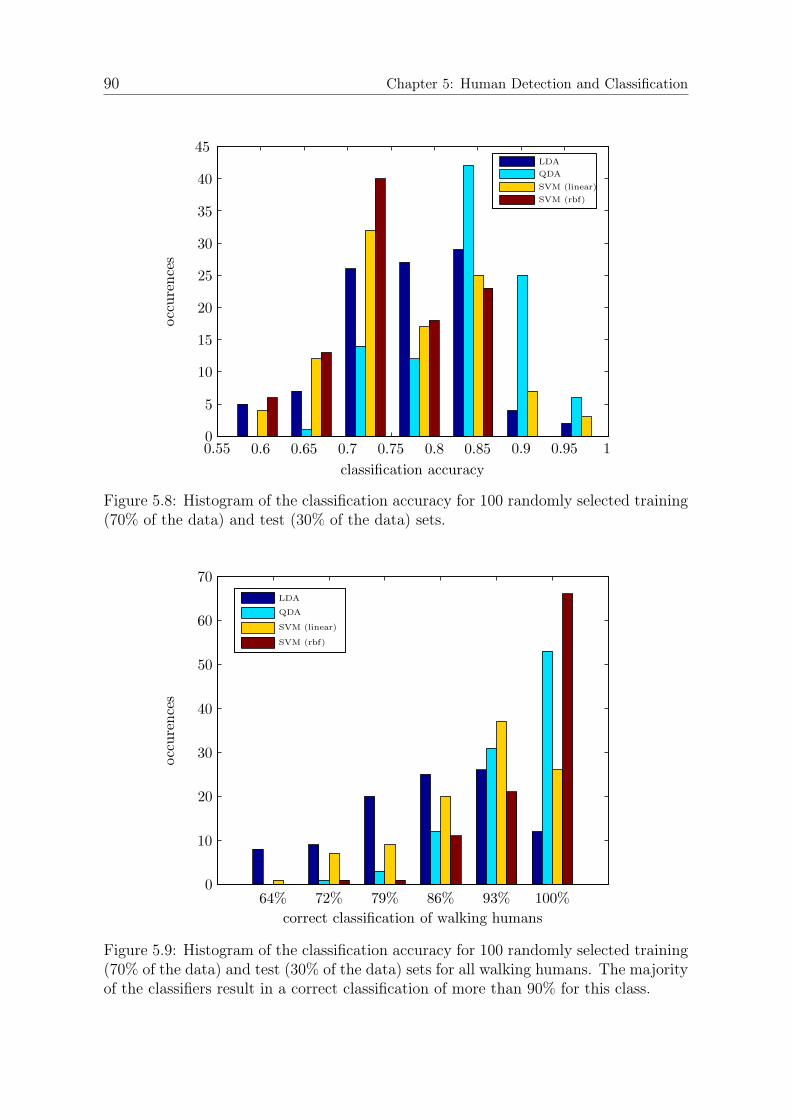
90 Chapter 5: Human Detection and Classification
Figure 5.8: Histogram of the classification accuracy for 100 randomly selected training(70% of the data) and test (30% of the data) sets.
Figure 5.9: Histogram of the classification accuracy for 100 randomly selected training(70% of the data) and test (30% of the data) sets for all walking humans. The majorityof the classifiers result in a correct classification of more than 90% for this class.

5.5 Results 91
classified asMethod total accuracy class W S
LDA 87.31%W 86.30% 13.70%S 10.96% 89.04%
QDA 91.89%W 100% 0%S 21.92% 78.08%
SVM (linear) 79.21%W 86.30% 13.70%S 32.88% 67.12%
SVM (rbf) 79.47%W 93.15% 6.85%S 43.84% 56.16%
Table 5.3: Classification performance of Linear Discriminant Analysis, Quadratic Dis-criminant Analysis and Support Vector Machines with linear and Gaussian kernels forthe classes of walking and standing humans using cross-validation.
of the elliptic fitting in order to detect aberrant shapes prior to the classification.Alternatively, using more training data will also improve the performance of the SVMssuch that they perform equally good or even better than the other classifiers.
92
Chapter 6
Conclusions and Outlook
This chapter presents an overview of the conclusions drawn from results in the precedingchapters as well as an outlook to possible future work.
6.1 Conclusions
In this thesis, we have discussed the design of active acoustic imaging systems usingacoustic arrays for general object detection tasks as well as object classification in thecontext of robotic applications. Acoustic imaging can greatly increase the reliabilityof scene analysis by offering and spatial resolution and direct range measurementsindependently of any other sensor entity. Furthermore, the echoes depend mainlyon the shape of an object, not its material. It is therefore possible to compensatelimitations and weaknesses of other sensors such as cameras, radar or lidar. Due totheir cheap costs and reliability even in most severe conditions, acoustic sensors canbe used for imaging and are a valuable tool in all situations where objects have to bedetected and analyzed. We have discussed basic principles of active acoustic imagingsystems that operate in air and presented an approach to calibrate acoustic arrays whichare affected by position errors and other, direction-independent errors using a methodthat overcomes some limitations of previous methods and is computationally simple.This allows the calibration of acoustic arrays using only a low number of calibrationsources. Due to the cost-sensitive nature of some applications, we also emphasized onthe problem of sparse array design. We presented approaches to design highly sparsearrays with good resolution and noise suppression capabilities and demonstrated theireffectiveness by both simulations and application to real data measurements. Theimages obtained using those sparse layouts show the significant echoes and shapes ofobjects in the scene. For large reflecting areas, the power reception can be altered.However, this is not affecting the ability to detect objects and model their shapesin a 3D fashion. On the functional level, we have developed features which allow areliable detection of persons and distinguishes them from other objects. The obtainedclassifiers allow correct classification of human and non-human objects with a rate ofalmost 97 percent. Furthermore, we have shown that it is possible to classify the poseof a person even further, e.g., we presented a feature set which allows to distinguishbetween walking and standing persons using not only geometrical features, but also
6.2 Outlook 93
statistical features obtained from the time-series data of the system. The features havebeen chosen using a feature selection method based on mutual information criteria.Based on this feature set, a correct classification rate of 87−90 percent can be achieved.
6.2 Outlook
The system used throughout this work was so far limited to narrowband excitationsignals. Therefore, it is worthwhile to consider broadband excitation which is expectedto allow even higher spatial resolution, if needed. Additionally, the obtained echoesfrom the objects could be analyzed for different frequencies which extends the possi-bilities to infer information about texture and shape of the objects. Another intuitivestep to take of the presented work is the extension to dynamic scenes, i.e., to trackobjects over time. This would allow infer more information about more complicatedobjects or estimate and predict trajectories in a scene. By analyzing echoes obtainedfrom different viewing angles, it could be possible to obtain a more precise model of thereflecting objects and model the surrounding scene of the platform more accurately.With respect to sparse array design, a natural extension of the presented methodswould be to apply the design concepts to 3D arrays. In that context, the pressure ofreducing the number of sensors is even higher, and we expect similar gains in sparsityby applying the theory of array redundancy and controlled manipulation thereof. Itwould also be worthwhile to analyze the relation between the non-uniformity of arraysand their performance in application-specific figures of merit. For example, some ap-plications of acoustic imaging require a reliable detection not only of the object it self,but also its shape. Simply using the mean square error (MSE) in such situations isnot sufficient and it would be beneficial to have a an effective way of measuring whatthe effect of an increased sparsity of the array is in terms of reduced quality of shaperepresentation. On the other hand, in DOA estimation problems, the effect of sparsitycan not be measured by the Cramer-Rao-Bound, but more general bounds have to betaken into account. With a more general figure of merit, one could more easily designarrays with maximal sparsity, if the desired estimation accuracy is known.
The presented results on human presence detection and classification can be extendedto other classes. For example, it should be possible to classify the pose of a humannot only by movement, but also by the orientation relative to the array, e.g., whetherthe person is facing the platform or looking to left, to the right or away from theplatform. Moreover, it might be possible to even recognize simple gestures in 3D andtherefore improve the gesture recognition of a robot by combining acoustic imaging withoptical cameras. As stated above, also the classification of dynamic scenes is possible

94 Chapter 6: Conclusions and Outlook
and the classifier could be integrated in a framework to obtain reliable detection andclassification results over a period of time.
95
Bibliography
[AGGS96] Y. I. Abramovich, D. A. Gray, A. Y. Gorokhov, and N. K. Spencer. Com-parison of doa estimation performance for various types of sparse antennaarray geometries. In Proceedings of the EUSIPCO, 1996.
[AGGS98] Y.I. Abramovich, D.A. Gray, A.Y. Gorokhov, and N.K. Spencer. Positive-definite Toeplitz completion in DOA estimation for nonuniform linearantenna arrays. I. fully augmentable arrays. IEEE Trans. Signal Process.,46(9):2458–2471, 1998.
[AH02] A. Austeng and S. Holm. Sparse 2-D arrays for 3-D phased array imaging- design methods. IEEE Trans. Ultrason., Ferroelectr., Freq. Control,49(8):1073–1086, Aug 2002.
[AHW+97] A. Austeng, S. Holm, P.K. Weber, N. Aakvaag, and K. Iranpour. 1D and2D algorithmically optimized sparse arrays. In Proceedings of the IEEEUltrasonics Symposium, volume 2, pages 1683–1686 vol.2, 1997.
[Aka74] H. Akaike. A new look at the statistical model identification. IEEE Trans.Autom. Control, AC 19:716–723, 1974.
[AS72] M Abramowitz and I A Stegun. Handbook of mathematical functionswith formulas, graphs, and mathematical tables, 1972.
[ASG99a] Y.I. Abramovich, N.K. Spencer, and A.Y. Gorokhov. Positive-definiteToeplitz completion in DOA estimation for nonuniform linear antennaarrays. II. partially augmentable arrays. IEEE Trans. Signal Process.,47(6):1502–1521, 1999.
[ASG99b] Y.I. Abramovich, N.K. Spencer, and A.Y. Gorokhov. Resolving mani-fold ambiguities in direction-of-arrival estimation for nonuniform linearantenna arrays. IEEE Trans. Signal Process., 47(10):2629–2643, 1999.
[AW89] A.S. Acampora and J.H. Winters. Three-dimensional ultrasonic vision forrobotic applications. IEEE Trans. Pattern Anal. Mach. Intell., 11(3):291–303, 1989.
[BB99] Dimitri P. Bertsekas and Dimitri P. Bertsekas. Nonlinear Programming.Athena Scientific, 2nd edition, September 1999.
[Bed86] S.D. Bedrosian. Nonuniform linear arrays: Graph-theoretic approach tominimum redundancy. Proc. of the IEEE, 74(7):1040–1043, 1986.
[BH09] Nicola Bellotto and Huosheng Hu. Multisensor-based human detectionand tracking for mobile service robots. IEEE Trans. Syst., Man, Cybern.B, 39(1):167–181, 2009.
[BI98] A. Blake and M. Isard. Active Contours: The Application of Techniquesfrom Graphics,Vision,Control Theory and Statistics to Visual Tracking ofShapes in Motion. Springer-Verlag New York, Inc., New York, USA, 1998.
96 Bibliography
[Bis07] C. M. Bishop. Pattern Recognition and Machine Learning. Springer, 1stedition, October 2007.
[BK04] Y. Boykov and V. Kolmogorov. An experimental comparison of min-cut/max- flow algorithms for energy minimization in vision. IEEE Trans.Pattern Anal. Mach. Intell., 26(9):1124–1137, 2004.
[Boh88] D.A. Bohn. Environmental effects on the speed of sound. J. of AudioEngineering, 36(4):223–231, April 1988.
[BV98] K.L. Bell and H.L. Van Trees. Adaptive beamforming for spatially spreadsources. In Proceedings of the Ninth IEEE SP Workshop on StatisticalSignal and Array Processing, pages 1–4, 1998.
[Cab08] Cabinet Office of Japan. Strategy for innovative technology. Technicalreport, Council for Science and Technology Policy, 2008.
[Cap69] J. Capon. High-resolution frequency-wavenumber spectrum analysis. Pro-ceedings of the IEEE, 57(8):1408–1418, 1969.
[CD00] R. Cutler and L.S. Davis. Robust real-time periodic motion detection,analysis, and applications. IEEE Trans. Pattern Anal. Mach. Intell.,22(8):781–796, 2000.
[CJS93] Z.-H. Cho, J. P. Jones, and M. Singh. Foundations of Medical Imaging.Wiley, New York, 1993.
[CST00] N. Cristianini and J. Shawe-Taylor. An introduction to Support VectorMachines. Cambridge University Press, March 2000.
[CV01] T.F. Chan and L.A. Vese. Active contours without edges. IEEE Trans.Image Process., 10(2):266–277, 2001.
[CZO87] H. Cox, R. Zeskind, and M. Owen. Robust adaptive beamforming. IEEETrans. Acoust., Speech, Signal Process., 35(10):1365– 1376, Oct 1987.
[DD94a] M.A. Doron and E. Doron. Wavefield modeling and array processing, parti - spatial sampling. IEEE Trans. Signal Process., 42(10):2549–2559, Oct1994.
[DD94b] M.A. Doron and E. Doron. Wavefield modeling and array processing, partii - algorithms. IEEE Trans. Signal Process., 42(10):2560–2570, Oct 1994.
[DD94c] M.A. Doron and E. Doron. Wavefield modeling and array processing, partiii - resolution capacity. IEEE Trans. Signal Process., 42(10):2571–2580,Oct 1994.
[DHS01] R.O. Duda, P.E. Hart, and D.G. Stork. Pattern Classification. Wiley,New York, 2001.
[DLR77] A. P. Dempster, N. M. Laird, and D. B. Rubin. Maximum likelihood fromincomplete data via the EM algorithm. Journal of the Royal StatisticalSociety. Series B (Methodological), 39(1):1–38, 1977.

Bibliography 97
[DLX00] K.R. Dandekar, H. Ling, and G. Xu. Smart antenna array calibrationprocedure including amplitude and phase mismatch and mutual couplingeffects. In IEEE International Conference on Personal Wireless Commu-nications, pages 293–297, 2000.
[EJS82] J.E. Evans, J.R. Johnson, and D.F. Sun. High resolution angular spec-trum estimation techniques for terrain scattering analysis and angle ofarrival estimation in atc navigation and surveillance system. TechnicalReport 582, MIT Lincoln Lab, Lexington, MA, 1982.
[FD96] A. Fenster and D.B. Downey. 3-D ultrasound imaging: a review. IEEEEngineering in Medicine and Biology Magazine, 15(6):41–51, 1996.
[fE10] United Nations Economic Commission for Europe. Statistical database -road accidents by accident type, light condition, country and year, 2010.
[FF95] Andrew Fitzgibbon and Robert B. Fisher. A buyer’s guide to conic fitting.In In British Machine Vision Conference, pages 513–522, 1995.
[FPF99] A. Fitzgibbon, M. Pilu, and R.B. Fisher. Direct least square fitting ofellipses. IEEE Trans. Pattern Anal. Mach. Intell., 21(5):476–480, 1999.
[FW92] B. Friedlander and A.J. Weiss. Direction finding using spatial smoothingwith interpolated arrays. IEEE Trans. Aerosp. Electron. Syst., 28(2):574–587, 1992.
[GCB+08] S. Gidel, P. Checchin, C. Blanc, T. Chateau, and L. Trassoudaine. Pedes-trian detection method using a multilayer laserscanner: Application inurban environment. In International Conference on Intelligent Robotsand Systems, pages 173–178, 2008.
[GGS94] W. Gander, G.H. Golub, and R. Strebel. Least-squares fitting of circlesand ellipses. BIT Numerical Mathematics, 43(4):558–578, Dec 1994.
[HAIH01] S. Holm, A. Austeng, K. Iranpour, and J.-F. Hopperstad. NonuniformSampling - Theory and Practice, chapter 19, pages 787–833. Kluwer, NewYork, 2001.
[HB91] Y.D. Huang and M. Barkat. Near-field multiple source localization bypassive sensor array. IEEE Trans. Antennas Propag., 39(7):968–975, 1991.
[Hen91] W.J. Hendricks. The totally random versus the bin approach for randomarrays. IEEE Trans. Antennas Propag., 39(12):1757–1762, 1991.
[Hil75] B.M. Hill. A simple general approach to inference about the tail of adistribution. The Annals of Statistics, 3(5):1163–1174, Sep. 1975.
[HJOK85] S. Haykin, J.H. Justice, N.L. Owsley, and A.C. Kak. Array Signal Pro-cessing. Prentice-Hall, New Jersey, USA, 1985.
98 Bibliography
[HMJG06] M. Heckmann, M. Moebus, F. Joublin, and C. Goerick. Speaker indepen-dent voiced-unvoiced detection evaluated in different speaking styles. InProc. of Interspeech 2006, International Conference on Spoken LanguageProcessing, Pittsburgh, USA, September 2006.
[Hol00] S. Holm. Sparse and irregular sampling in array processing. In Proc.of the IEEE International Conference on Acoustics, Speech, and SignalProcessing, volume 6, pages 3850–3853 vol.6, 2000.
[Hsi99] P.-H. Hsieh. Robustness of tail index estimation. Journal of Computa-tional and Graphical Statistics, 8(2):318–332, 1999.
[Hun00] E.K.L. Hung. Matrix-construction calibration method for antenna arrays.IEEE Trans. Aerosp. Electron. Syst., 36(3):819–828, 2000.
[ISO10] ISO 17386:2010: Transport information and control systems – manoeu-vring aids for low speed operation (MALSO) – performance requirementsand test procedures, 2010.
[JPAE09] Graziella Jost, Marco Popolizio, Richard Allsop, and Vojtech Eksler. 3rdroad safety annual report - 2010 on the horizon. Technical report, Euro-pean Transport Safety Council (ETSC), 2009.
[JRS07] N. Jin and Y. Rahmat-Samii. Advances in particle swarm optimizationfor antenna designs: Real-number, binary, single-objective and multiob-jective implementations. IEEE Trans. Antennas Propag., 55(3):556–567,2007.
[JZ97] A. Jain and D. Zongker. Feature selection: evaluation, application, andsmall sample performance. IEEE Trans. Pattern Anal. Mach. Intell.,19(2):153–158, 1997.
[Kop92] L.E. Kopilovich. New approach to constructing two-dimensional aperturesynthesis systems. IEE Proc. F, Radar and Signal Processing, 139(5):365–368, 1992.
[Kop08] L. E. Kopilovich. Square array antennas based on Hadamard differencesets. IEEE Trans. Antennas Propag., 56(1):263–266, Jan 2008.
[KS91] L.E. Kopilovich and L.G. Sodin. Two-dimensional aperiodic antenna ar-rays with a low sidelobe level. IEE Proc. H, Microwaves, Antennas andPropagation, 138(3):233–237, 1991.
[KV96] H. Krim and M. Viberg. Two decades of array signal processing research.IEEE Signal Process. Mag., 13(4):67–94, 1996.
[KWT88] Michael Kass, Andrew Witkin, and Demetri Terzopoulos. Snakes: Ac-tive contour models. INTERNATIONAL JOURNAL OF COMPUTERVISION, 1(4):321–331, 1988.
[Lee56] J. Leech. On the representation of 1, 2, ..., n by differences. J. of theLondon Mathematical Society, 31:160–169, 1956.
Bibliography 99
[Lee99] D.G. Leeper. Isophoric arrays-massively thinned phased arrays with well-controlled sidelobes. IEEE Trans. Antennas Propag., 47(12):1825–1835,Dec 1999.
[Lie09] Bernd Liepert. The strategic research agenda for robotics in europe. Tech-nical report, European Robotics Technoloy Platform, 2009.
[Lin92] D.A. Linebarger. A fast method for computing the coarray of sparse lineararrays. IEEE Trans. Antennas Propag., 40(9):1109–1112, 1992.
[Lit09] Gudrun Litzenberger. World robotics. Technical report, InternationalFederation of Robotics, 2009.
[LLV06] M. Lanne, A. Lundgren, and M. Viberg. Calibrating an array with scandependent errors using a sparse grid. In Fortieth Asilomar Conference onSignals, Systems and Computers (ACSSC), pages 2242–2246, 2006.
[Lo63] Y. Lo. A probabilistic approach to the design of large antenna arrays.IEEE Trans. Antennas Propag., 11(1):95–96, 1963.
[Lo64] Y. Lo. A mathematical theory of antenna arrays with randomly spacedelements. IEEE Trans. Antennas Propag., 12(3):257–268, 1964.
[LST93] D.A. Linebarger, I.H. Sudborough, and I.G. Tollis. Difference bases andsparse sensor arrays. IEEE Trans. Inf. Theory, 39(2):716–721, 1993.
[LSW03] J. Li, P. Stoica, and Z. Wang. On robust capon beamforming and diagonalloading. IEEE Trans. Signal Process., 51(7):1702–1715, 2003.
[LTB98] G.R. Lockwood, J.R. Talman, and S.S. Brunke. Real-time 3-D ultrasoundimaging using sparse synthetic aperture beamforming. IEEE Trans. Ul-trason., Ferroelectr., Freq. Control, 45(4):980–988, 1998.
[LVL05] B.K. Lau, M. Viberg, and Y.-H. Leung. Data-adaptive array interpo-lation for DOA estimation in correlated signal environments. In IEEEInt. Conf. Acoustics, Speech, and Signal Processing (ICASSP), volume 4,pages iv/945–iv/948 Vol. 4, 2005.
[LVL07] M. Lanne, M. Viberg, and A. Lundgren. Adaptive beamforming using cal-ibration vectors with unknown gain and phase. IEEE Antennas and Prop-agation Society International Symposium, pages 4208–4211, June 2007.
[LWLW06] Z. Li, K. Wang, L. Li, and F.-Y. Wang. A review on vision-based pedes-trian detection for intelligent vehicles. In Vehicular Electronics and Safety,2006. ICVES 2006. IEEE International Conference on, pages 57–62, 2006.
[Mar86] F. Marvasti. Signal recovery from nonuniform samples and spectral analy-sis on random nonuniform samples. In IEEE Int. Conf. Acoustics, Speech,and Signal Processing (ICASSP), volume 11, pages 1649–1652, 1986.
[MC90] F.A. Marvasti and L. Chuande. Parseval relationship of nonuniform sam-ples of one- and two-dimensional signals. IEEE Trans. Acoust., Speech,Signal Process., 38(6):1061–1063, 1990.
100 Bibliography
[MD01] Y. Meurisse and J.-P. Delmas. Bounds for sparse planar and volumearrays. IEEE Trans. Inf. Theory, 47(1):464–468, 2001.
[Mof68] A. Moffet. Minimum-redundancy linear arrays. IEEE Trans. AntennasPropag., 16(2):172–175, 1968.
[MT94] V. Murino and A. Trucco. Underwater 3D imaging by FFT dynamicfocusing beamforming. In Image Processing, 1994. Proc.. ICIP-94., IEEEInternational Conference, volume 1, pages 890–894 vol.1, 1994.
[MT00] V. Murino and A. Trucco. Three-dimensional image generation and pro-cessing in underwater acoustic vision. Proc. of the IEEE, 88(12):1903–1948, 2000.
[MVZ10] M. Moebus, M. Viberg, and A.M. Zoubir. Parametrization of acousticimages for the detection of human presence by mobile platforms. In Proc.of the IEEE Int’l Conference on Acoustics, Speech and Signal Processing,2010.
[MWW96] Yan Meng, Kon Max Wong, and Qiang Wu. Direction finding for pointand dispersed sources: VEC-MUSIC and its performance. In IEEE In-ternational Conference on Acoustics, Speech, and Signal Processing, vol-ume 5, pages 2908–2911, 1996.
[Myo09] Yumiko Myoken. Research and development for next generation servicerobots in japan. Technical report, British Embass Japan, Science andInnovation Sectio, Jan 2009.
[MZ07a] M. Moebus and A.M. Zoubir. A comparison of beamforming algorithmsfor 3D ultrasound imaging in air. In Proceedings of the 3rd Biennial onDSP for In-Vehicle and Mobile Systems, Istanbul, Turkey, June 2007.
[MZ07b] M. Moebus and A.M. Zoubir. Three-dimensional ultrasound imaging inair using a 2D array on a fixed platform. In Proc. of the IEEE Int’lConference on Acoustics, Speech and Signal Processing, volume 2, pagesII–961–II–964, 2007.
[MZ08a] M. Moebus and A.M. Zoubir. 2D nonuniform array design for imagingapplications. In Proc. of the Int’l ITG Workshop on Smart Antennas(WSA), pages 180 – 183, Darmstadt, Germany, Februar 2008.
[MZ08b] M. Moebus and A.M. Zoubir. In-Vehicle Corpus and Signal Processingfor Driver Behavior, chapter 13, pages 147–159. Springer, 2008.
[MZ08c] M. Moebus and A.M. Zoubir. On the design of sparse arrays using differ-ence sets. In Proc. of the 5th IEEE Sensor Array and Multichannel SignalProcessing Workshop (SAM), pages 247–251, Darmstadt, Germany, 2008.
[MZ09a] M. Moebus and A.M. Zoubir. Local array calibration using parametricmodeling of position errors and a sparse calibration grid. In Proc. of theInt’l IEEE Workshop on Statistical Signal Processing, Cardiff, Wales, UK,Sep 2009.
Bibliography 101
[MZ09b] M. Moebus and A.M. Zoubir. Verfahren zum Entwerfen einer Anordnungvon Sensoren, 2009. in application phase, app.-no. 10 2009 044 230.8.
[MZ10a] M. Moebus and A.M. Zoubir. Detection and classification of humansusing acoustic imaging. Pattern Recognition, 2010. under review.
[MZ10b] M. Moebus and A.M. Zoubir. Ultrasound object detection using 2D sparsearrays with low sidelobes. Signal Processing, 2010. under review.
[NS96] B. C. Ng and C. M. S. See. Sensor-array calibration using a maximum-likelihood approach. IEEE Trans. Antennas Propag., 44(6):827–835, 1996.
[NW99] Jorge Nocedal and Stephen J. Wright. Numerical Optimization. SpringerSeries in Operations Research. Springer, New York, 2nd edition, July1999.
[OM05] U. Oktel and R.L. Moses. A Bayesian approach to array geometry design.IEEE Trans. Signal Process., 53(5):1919–1923, May 2005.
[OV91] B. Ottersten and M. Viberg. Local modeling and robust estimation forhigh-resolution direction finding. In Conference Record of the Twenty-Fifth Asilomar Conference on Signals, Systems and Computers, volume 2,pages 1005–1009, 1991.
[PBNH85] S.U. Pillai, Y. Bar-Ness, and F. Haber. A new approach to array geom-etry for improved spatial spectrum estimation. Proceedings of the IEEE,73(10):1522–1524, Oct. 1985.
[PDM98] O.V. Pictet, M.M. Dacrorogna, and U.A. Müller. A practical guide toheavy tails: statistical techniques and applications, chapter 3, pages 283–310. Birkhäuser Boston Inc., Cambridge, MA, USA, 1998.
[PH96] D.J. Powell and G. Hayward. Flexible ultrasonic transducer arrays fornondestructive evaluation applications. I. The theoretical modeling ap-proach. IEEE Trans. Ultrason., Ferroelectr., Freq. Control, 43(3):385–392, 1996.
[PK91] J. Pierre and M. Kaveh. Experimental performance of calibration anddirection-finding algorithms. In IEEE Int. Conf. Acoustics, Speech, andSignal Processing (ICASSP), pages 1365–1368 vol.2, 1991.
[PLD05] H. Peng, F. Long, and C. Ding. Feature selection based on mutual infor-mation criteria of max-dependency, max-relevance, and min-redundancy.IEEE Trans. Pattern Anal. Mach. Intell., 27(8):1226–1238, 2005.
[PPL90] D. Pearson, S.U. Pillai, and Y. Lee. An algorithm for near-optimal place-ment of sensor elements. IEEE Trans. Inf. Theory, 36(6):1280–1284, 1990.
[Ric07] C.D. Richmond. Cross coherence and joint pdf of the bartlett and caponpower spectral estimates. In IEEE International Conference on Acoustics,Speech and Signal Processing, volume 2, pages II–901–II–904, 2007.
102 Bibliography
[Ric10] C.D. Richmond. Statistical analysis of capon-bartlett 2-d cross spectrum.In IEEE International Conference on Acoustics, Speech and Signal Pro-cessing, 2010.
[RL75] W. Richards and Yuen Lo. Antenna pattern synthesis based on optimiza-tion in a probabilistic sense. IEEE Trans. Antennas Propag., 23(2):165–172, 1975.
[Ruf93] C.S. Ruf. Numerical annealing of low-redundancy linear arrays. IEEETrans. Antennas Propag., 41(1):85–90, 1993.
[RW84] Richard A. Redner and Homer F. Walker. Mixture densities, maximumlikelihood and the EM algorithm. SIAM Review, 26(2):195–239, Apr.,1984.
[SC08] Ingo Steinwart and Andreas Christmann. Support Vector Machines.Springer, 2008.
[Sch86] R. Schmidt. Multiple emitter location and signal parameter estimation.IEEE Trans. Antennas Propag., 34(3):276–280, 1986.
[Set99] J. A. Sethian. Level Set Methods and Fast Marching Methods: Evolv-ing Interfaces in Computational Geometry, Fluid Mechanics, ComputerVision, and Materials Science. Cambridge University Press, June 1999.
[SK85] T.-J. Shan and T. Kailath. Adaptive beamforming for coherent signalsand interference. IEEE Trans. Acoust., Speech, Signal Process., 33(3):527– 536, Jun 1985.
[SK92] A. L. Swindlehurst and T. Kailath. A performance analysis of subspace-based methods in the presence of model errors. I. The MUSIC algorithms.IEEE Trans. Signal Process., 40(7):1758–1774, July 1992.
[SK93] A. L. Swindlehurst and T. Kailath. A performance analysis of subspace-based methods in the presence of model error. II. Multidimensional algo-rithms. IEEE Trans. Signal Process., 41(9):2882–2890, Sept. 1993.
[SS98] A. L. Swindlehurst and P. Stoica. Maximum likelihood methods in radararray signal processing. Proc. IEEE, 86(2):421–441, Feb. 1998.
[SS04] P. Stoica and Y. Selen. Model-order selection: a review of informationcriterion rules. IEEE Signal Process. Mag., 21(4):36–47, 2004.
[Ste72] B. Steinberg. The peak sidelobe of the phased array having randomlylocated elements. IEEE Trans. Antennas Propag., 20(2):129–136, 1972.
[Ste00] S. Stergiopoulos. Advanced Signal Processing Handbook: Theory and Im-plementation for Radar, Sonar, and Medical Imaging Real-Time Systems.CRC Press, Inc., 2000.
Bibliography 103
[STI08] Go Shingu, Kenichi Takizawa, and Tetushi Ikegami. Human body de-tection using mimo-uwb radar sensor network in an indoor environment.International Conference on Parallel and Distributed Computing Appli-cations and Technologies, 0:437–442, 2008.
[SWK85] T.-J. Shan, M. Wax, and T. Kailath. On spatial smoothing for direction-of-arrival estimation of coherent signals. IEEE Trans. Acoust., Speech,Signal Process., 33(4):806 – 811, Aug 1985.
[Tap02] M. Tapio. Direction and spread estimation of spatially distributed signalsvia the power azimuth spectrum. In IEEE Int. Conf. Acoustics, Speech,and Signal Processing (ICASSP), volume 3, pages 3005–3008, 2002.
[TBPI10] F.H.C. Tivive, A. Bouzerdoum, S.L. Phung, and K.M. Iftekharuddin.Adaptive hierarchical architecture for visual recognition. Appl. Opt.,49(10):B1–B8, April 2010.
[TDMO04] M. Tons, R. Doerfler, M.-M. Meinecke, and M.A. Obojski. Radar sen-sors and sensor platform used for pedestrian protection in the ec-fundedproject save-u. In Intelligent Vehicles Symposium, 2004 IEEE DOI -10.1109/IVS.2004.1336489, pages 813–818, 2004.
[Tru99] A. Trucco. Thinning and weighting of large planar arrays by simulatedannealing. IEEE Trans. Ultrason., Ferroelectr., Freq. Control, 46(2):347–355, 1999.
[Van02] H. L. Van Trees. Detection, Estimation and Modulation Theory Part IV- Optimum Array Signal Processing, volume 4. Wiley, 2002.
[Vib10] M. Viberg. Error modeling and calibration for high resolution doa esti-mation. Signal Processing, 90(5):279–282, May 2010.
[VO91] M. Viberg and B. Ottersten. Sensor array processing based on subspacefitting. IEEE Trans. Signal Process., 39(5):1110–1121, 1991.
[VS94a] M. Viberg and A. L. Swindlehurst. Analysis of the combined effects offinite samples and model errors on array processing performance. IEEETrans. Signal Process., 42(11):3073–3083, Nov. 1994.
[VS94b] M. Viberg and A.L. Swindlehurst. A Bayesian approach to auto-calibration for parametric array signal processing. IEEE Trans. SignalProcess., 42(12):3495–3507, 1994.
[VVB88] B.D: Van Veen and K.M. Buckley. Beamforming: A versatile approachto spatial filtering. IEEE ASSP Mag., 5(2):4–24, 1988.
[WF93] A.J. Weiss and B. Friedlander. Performance analysis of spatial smoothingwith interpolated arrays. IEEE Trans. Signal Process., 41(5):1881–1892,1993.
[WHO09] Global status report on road safety, 2009.

104 Bibliography
[WK85] M. Wax and T. Kailath. Detection of signals by information theoreticcriteria. IEEE Trans. Acoust., Speech, Signal Process., 33(2):387 – 392,1985.
[WWMR94] Q. Wu, K.M. Wong, Y. Meng, and W. Read. DOA estimation of pointand scattered sources - VET-MUSIC. In IEEE Seventh SP Workshop onStatistical Signal and Array Processing, pages 365–368, 1994.
[WZ88] M. Wax and I. Ziskind. Detection of fully correlated signals by themdl principle. IEEE Int. Conf. Acoustics, Speech, and Signal Process-ing (ICASSP), 5:2777 – 2780, 1988.
[WZ89] M. Wax and I. Ziskind. Detection of the number of coherent signals by themdl principle. IEEE Trans. Acoust., Speech, Signal Process., 37(8):1190– 1196, 1989.
[YTN05] N. Yamada, Y. Tanaka, and K. Nishikawa. Radar cross section for pedes-trian in 76GHz band. In European Microwave Conference, volume 2, Oct.2005.
[ZL04] D. Zhang and G. Lu. Review of shape representation and descriptiontechniques. Pattern Recognition, 37(1):1–19, 2004.

105
Curriculum Vitae
Education & Work Experience
Since Oct. 2010 Project Leader Advanced Active SafetyGeneral Motors Europe, Adam Opel GmbHRüsselsheim, Germany
July 2009 Visiting researcher at the division "Signal Processing & Antennas”,Department of Signals & Systems, Chalmers University of TechnologyGöteborg, Sweden
Apr. 2006 - Sep. 2010 Research Associate at the Signal Processing Group,Institute of Telecommunications, Technische Universität DarmstadtDarmstadt, Germany
Feb. 2006 - Mar. 2006 Visitor at the Communications and Signal Processing Lab,Curtin University of TechnologyPerth, Australia
Oct. 2005 Diploma (Dipl.-Wirtsch.-Ing.) for the combined studies ofelectrical engineering and business administration,Technische Universität DarmstadtDarmstadt, GermanyGrade "very good" (1.4)
Apr. 2006 - Sep. 2010 Diploma thesis on "Speaker-independent Voiced/UnvoicedDetection in Spontaneous and Read Speech"Honda Research Institute Europe, Offenbach, Germany
Apr. 2006 - Sep. 2010 Study thesis on "Finance problems in project portfolio management" ,at Campana & Schott, Frankfurt, Germany
Dec. 2003 - Apr. 2004 Study thesis on "Detection of Digital Watermarks inGeodetic Map Data Using the Bootstrap”Institute of Telecommunications, Technische Universität DarmstadtDarmstadt, Germany
Okt. 1999 - Mar 2002 Study of electrical engineering and business administrationTechnische Universität Darmstadt, Darmstadt, Germany(Vordiplom "good”, 2nd best of class)
Apr. 2006 - Sep. 2010 Abitur at Elly-Heuss-Gymnasium, WiesbadenGrade 1.1

107
Publications
A.1 Internationally Refereed Publications
• M. Heckmann, M. Moebus, F. Joublin, and C. Goerick. Speaker independentvoiced-unvoiced detection evaluated in different speaking styles. In Proc. of In-terspeech 2006, International Conference on Spoken Language Processing, Pitts-burgh, USA, September 2006
• M.Moebus and A.M. Zoubir. Three-dimensional ultrasound imaging in air using a2D array on a fixed platform. In Proc. of the IEEE Int’l Conference on Acoustics,Speech and Signal Processing, volume 2, pages II–961–II–964, 2007
• M. Moebus and A.M. Zoubir. A comparison of beamforming algorithms for 3Dultrasound imaging in air. In Proceedings of the 3rd Biennial on DSP for In-Vehicle and Mobile Systems, Istanbul, Turkey, June 2007
• M. Moebus and A.M. Zoubir. 2D nonuniform array design for imaging applica-tions. In Proc. of the Int’l ITG Workshop on Smart Antennas (WSA), pages 180– 183, Darmstadt, Germany, Februar 2008
• M. Moebus and A.M. Zoubir. In-Vehicle Corpus and Signal Processing for DriverBehavior, chapter 13, pages 147–159. Springer, 2008
• M. Moebus and A.M. Zoubir. On the design of sparse arrays using differencesets. In Proc. of the 5th IEEE Sensor Array and Multichannel Signal ProcessingWorkshop (SAM), pages 247–251, Darmstadt, Germany, 2008
• M. Moebus and A.M. Zoubir. Local array calibration using parametric model-ing of position errors and a sparse calibration grid. In Proc. of the Int’l IEEEWorkshop on Statistical Signal Processing, Cardiff, Wales, UK, Sep 2009
• M. Moebus, M. Viberg, and A.M. Zoubir. Parametrization of acoustic images forthe detection of human presence by mobile platforms. In Proc. of the IEEE Int’lConference on Acoustics, Speech and Signal Processing, 2010
• M. Moebus and A.M. Zoubir. Ultrasound object detection using 2D sparse arrayswith low sidelobes. Signal Processing, 2010. under review
• M. Moebus and A.M. Zoubir. Detection and classification of humans using acous-tic imaging. Pattern Recognition, 2010. under review
A.2 Filed Patent Applications
• M. Moebus and A.M. Zoubir. Verfahren zum Entwerfen einer Anordnung vonSensoren, 2009. in application phase, app.-no. 10 2009 044 230.8