Objective

To provide an introduction to the exciting and frustrating world of MATLAB.

Overview

The ancients created a programming environment to manipulate vectors and matrices.They (Mathworks) named it MATLAB which stands for MATrix LABoratory not to beconfused with MATLAV (MATrix LAVatory) a program for flushing matrices down thetoilet. MATLAB is a sophisticated numerical software package in the same vein as itscompetitor Mathematica. It includes advanced numerical algorithms and highly developvisualization tools which makes it very useful in solving and simulating complex systemsof equations. In addition, it uses a high-level programming language that allows users toquickly code and manipulate data.

Why use MATLAB

Matrices. Anything that is a vector or matrix is in the wheelhouse of MATLAB. With itsbuilt-in graphics capabilities, it is very easy to quickly analyze data and generate results.Other packages often require a bit more effort to manipulate data and visualize it, andmany more have copied MATLAB’s approach and style.

Common. MATLAB is widely used and thus enjoys a large community of support. Thelanguage is also copied by others like Octave and Julia which means that code can easilybe converted or shared.

Simulations. Many simulation techniques make use of vector and matrix formulationsand so MATLAB is very useful in large-scale simulations.

Ease. The high-level programming language of MATLAB means it is easy to code upan algorithm and fairly transparent to read/understand. There is also little overhead sovariables can be defined and modified on a whim, without prior declarations. No need totype “x = Int64[];”.

Debugging. MATLAB has two awesome features that assist in debugging and refiningcode. One are break points which temporarily stop code (even in functions) and allow theuser to check the state of various variables. The other is Profiler which computes the timeand number of calls of each segment of code within a program. Thus, it is easy to identifywhat is slowing down a program or what line is being called way too often.

Error messages. Perhaps this is person-specific but the error messages in MATLAB seemmuch clearer and easier to fix than certain other coding languages.

Why not to use MATLAB

Cost. MATLAB is a commercial product and as such costs money. It is cheaper forstudents but still has a price tag that many find prohibitive. Adding insult to injury, ittypically updates twice a year and these updates must be purchased separately. Fortu-nately, the basic language is the same but the performance can change.

1

2

Updates. As mentioned above, MATLAB frequently updates. Although this results inan overall improvement in performance, it can change the performance of user-written codebetween releases. It is not uncommon for codes to run slower and require reformatting torun faster– i.e. coding techniques may need to change with different releases.

Text processing. While MATLAB can handle strings and manipulate them, it is not itsstrong suit. MATLAB is quantitative and prefers to manipulate numbers. Languages likepython and perl are better options for this task.

Speed. MATLAB is faster than most languages but it is not the fastest. There is atradeoff to the user-friendly aspects of MATLAB and performance speed. For example,Julia code can be much faster than MATLAB (one pieces of code was 6X faster) but it canalso take longer to optimize Julia code.

Window Structure

MATLAB uses a collection of windows as part of its user interface. Each window containsdifferent types of information and can be removed or highlighted based on user desires.

(1) Current Folder: shows the contents of the current directory MATLAB is accessing.(2) Command Window: where most of the commands will be typed. It should probably

be the most prominent window.(3) Workspace: lists the variables currently defined and available.(4) Command History keeps track of the previous commands typed into the command

window.

They can be configured to individual preferences by messing around with the preferencessection. Basically, the Command Window and Workspace windows are the most useful/im-portant for regular programming.

Basics of the language

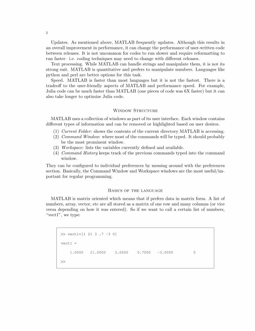
MATLAB is matrix oriented which means that if prefers data in matrix form. A list ofnumbers, array, vector, etc are all stored as a matrix of one row and many columns (or viceversa depending on how it was entered). So if we want to call a certain list of numbers,“vect1”, we type:

>> vect1=[1 21 3 .7 -3 0]

vect1 =

1.0000 21.0000 3.0000 0.7000 -3.0000 0

>>

3

Alternatively, if we did not want to write every element of a vector but just wanted aninterval starting at some number a increasing by δt and ending when b is reached, we wouldwrite vect2=[a:δt:b]. For instance:

>> vect2=[1:.2:2]

vect2 =

1.0000 1.2000 1.4000 1.6000 1.8000 2.0000

>> vect2=[1:.3:2]

vect2 =

1.0000 1.3000 1.6000 1.9000

>> vect2=[2:-.3:1]

vect2 =

2.0000 1.7000 1.4000 1.1000

>>

If we do not want MATLAB displaying the data then we simply put a semicolon atthe end of the line. Any line without a semicolon, is effectively asking MATLAB to printout the result of the code. This can be an eyesore and for certain codes can slow downperformance. Semicolons tell MATLAB, “Shut up.”

>> vect1=[1 21 3 .7 -3 0];>>

To access a certain element, say the third, from vect1, we simply type:

>> vect1(3)

ans =

3

>>

4

Note that MATLAB begins counting with 1 which means vect1(0) would return anerror. Furthermore, the results are stored as ans which means if we type ans+4 we get7. The Workspace window should also show the existence of a variable named ans. Toget the size (dimensionality) of vect1, we have two options. The first is using the built-infunction size and the second is the built-in function length.

>> size(vect1)

ans =

1 6

>> size(vect1,1)

ans =

1

>> size(vect1,2)

ans =

6

>> length(vect1)

ans =

6

>>

The function size displays the number of rows and then columns. It takes in onemandatory input, the item of which the size is requested. The second input, separated bya comma, is optional. It indicates whether one wants the number of rows (size( ,1)) orcolumns (size( ,2)). The function length reports back the biggest of the two dimen-sions, either row or column number. Dimensions is particularly important in MATLABand the cause of most errors. To make notation easier, we will say that a matrix withdimensions Z x Y (Z “by” Y) will have Z rows and Y columns (just like size reports).Using linear algebra, anything multiplied by this Z x Y must have Y as its first dimension.Thus, if a vector is to be multiplied by this matrix it must be Y x 1 and will return avector of Z x 1, i.e. (Z x Y) * (Y x 1) = (Z x 1). The “inner dimensions” must agree, i.e.

5

(Z x Y) * (Y x 1). This linear algebra fact forms the basis of MATLAB manipulations.Let’s try to square each element in vect1.

>> vect1*vect1Error using * Inner matrix dimensions must agree.

>>

This command did not work because the inner dimensions do not agree (1 x Y) * (1 xY), Y6= 1. One way to make it work is to transpose the second vect1 by adding a singleapostrophe after it vect1'. This changes it from a row vector (1 x Y) to a column vector(Y X 1) and gives (1 x Y) * (Y x 1 = 1 x 1. In other words, this is the dot product.Alternatively, we could transpose the first vect1 and get...?

>> vect1*(vect1')

ans =

460.4900

>>

To actually get a vector where each entry is the square of the corresponding entry invect1, we type:

>> vect1.*vect1

ans =

1.0000 441.0000 9.0000 0.4900 9.0000 0

>>

Any time a “.” appears before an operation it means “element-wise”, ignoring linearalgebra rules. So we can also use “.” with the exponent notation “ˆ”.

>> vect1.ˆ2

6

ans =

1.0000 441.0000 9.0000 0.4900 9.0000 0

>>

Here, are some other common commands with vectors in MATLAB.

>> sum(vect1)

ans =

22.7000

>> min(vect1)

ans =

-3

>> max(vect1)

ans =

21

>>

We could try taking the average of vect1.

>> average(vect1)Undefined function ’average’ for input arguments of type ’double’.

>>

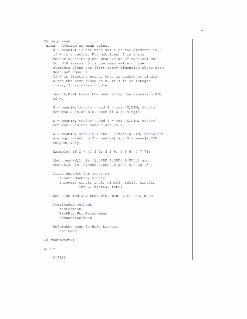
This error indicates that average is a function which does not exist in MATLAB. Isthere another way of doing it based on the functions presented so far? We can check tosee if another function exists using help.

7

>> help meanmean Average or mean value.

S = mean(X) is the mean value of the elements in Xif X is a vector. For matrices, S is a rowvector containing the mean value of each column.For N-D arrays, S is the mean value of theelements along the first array dimension whose sizedoes not equal 1.If X is floating point, that is double or single,S has the same class as X. If X is of integerclass, S has class double.

mean(X,DIM) takes the mean along the dimension DIMof X.

S = mean(X,'double') and S = mean(X,DIM,'double')returns S in double, even if X is single.

S = mean(X,'native') and S = mean(X,DIM,'native')returns S in the same class as X.

S = mean(X,'default') and S = mean(X,DIM,'default')are equivalent to S = mean(X) and S = mean(X,DIM)respectively.

Example: If X = [1 2 3; 3 3 6; 4 6 8; 4 7 7];

then mean(X,1) is [3.0000 4.5000 6.0000] andmean(X,2) is [2.0000 4.0000 6.0000 6.0000].'

Class support for input X:float: double, singleinteger: uint8, int8, uint16, int16, uint32,

int32, uint64, int64

See also median, std, min, max, var, cov, mode.

Overloaded methods:fints/meanProbDistUnivParam/meantimeseries/mean

Reference page in Help browserdoc mean

>> mean(vect1)

ans =

3.7833

8

>>

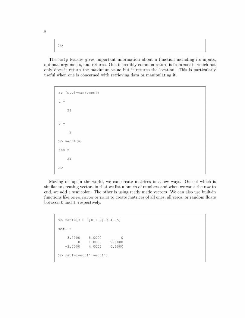
The help feature gives important information about a function including its inputs,optional arguments, and returns. One incredibly common return is from max in which notonly does it return the maximum value but it returns the location. This is particularlyuseful when one is concerned with retrieving data or manipulating it.

>> [u,v]=max(vect1)

u =

21

v =

2

>> vect1(v)

ans =

21

>>

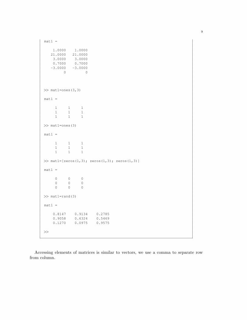
Moving on up in the world, we can create matrices in a few ways. One of which issimilar to creating vectors in that we list a bunch of numbers and when we want the row toend, we add a semicolon. The other is using ready made vectors. We can also use built-infunctions like ones,zeros,or rand to create matrices of all ones, all zeros, or random floatsbetween 0 and 1, respectively.

>> mat1=[3 8 0;0 1 9;-3 4 .5]

mat1 =

3.0000 8.0000 00 1.0000 9.0000

-3.0000 4.0000 0.5000

>> mat1=[vect1' vect1']

9

mat1 =

1.0000 1.000021.0000 21.00003.0000 3.00000.7000 0.7000

-3.0000 -3.00000 0

>> mat1=ones(3,3)

mat1 =

1 1 11 1 11 1 1

>> mat1=ones(3)

mat1 =

1 1 11 1 11 1 1

>> mat1=[zeros(1,3); zeros(1,3); zeros(1,3)]

mat1 =

0 0 00 0 00 0 0

>> mat1=rand(3)

mat1 =

0.8147 0.9134 0.27850.9058 0.6324 0.54690.1270 0.0975 0.9575

>>

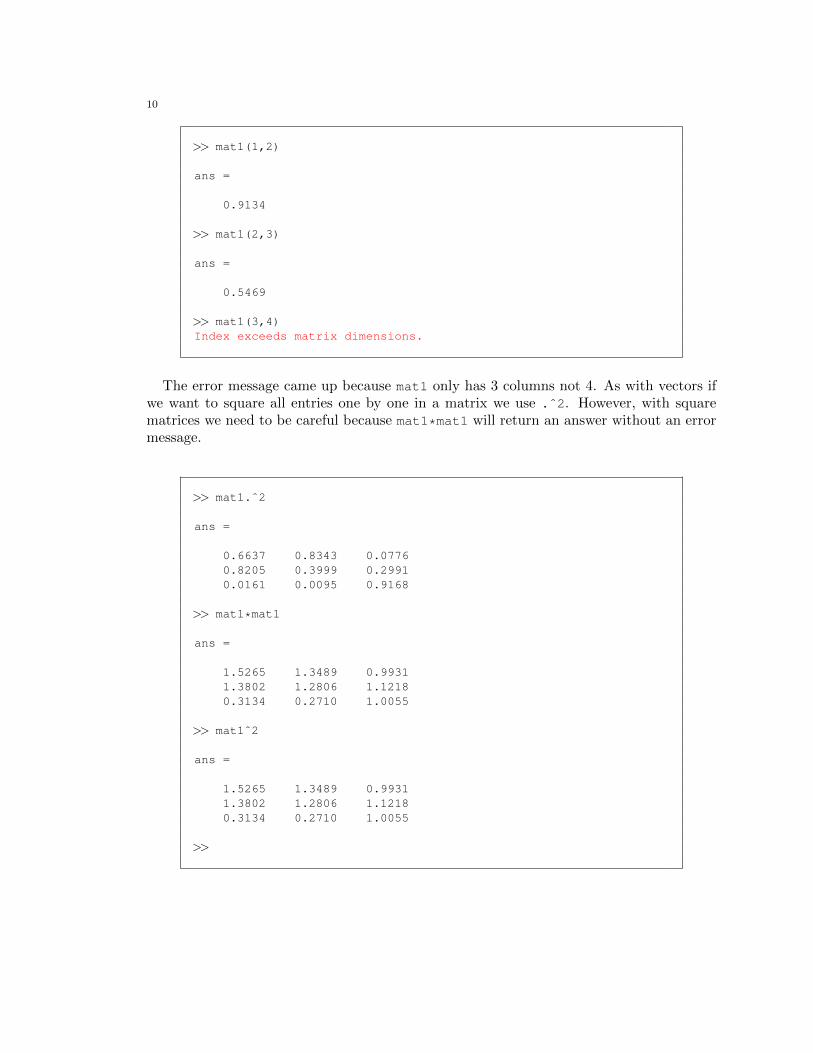
Accessing elements of matrices is similar to vectors, we use a comma to separate rowfrom column.

10

>> mat1(1,2)

ans =

0.9134

>> mat1(2,3)

ans =

0.5469

>> mat1(3,4)Index exceeds matrix dimensions.

The error message came up because mat1 only has 3 columns not 4. As with vectors ifwe want to square all entries one by one in a matrix we use .ˆ2. However, with squarematrices we need to be careful because mat1*mat1 will return an answer without an errormessage.

>> mat1.ˆ2

ans =

0.6637 0.8343 0.07760.8205 0.3999 0.29910.0161 0.0095 0.9168

>> mat1*mat1

ans =

1.5265 1.3489 0.99311.3802 1.2806 1.12180.3134 0.2710 1.0055

>> mat1ˆ2

ans =

1.5265 1.3489 0.99311.3802 1.2806 1.12180.3134 0.2710 1.0055

>>

11

Loading and saving data

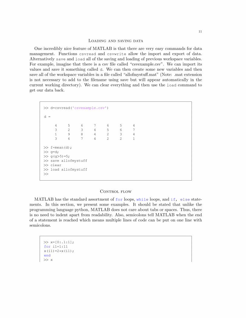
One incredibly nice feature of MATLAB is that there are very easy commands for datamanagement. Functions csvread and csvwrite allow the import and export of data.Alternatively save and load all of the saving and loading of previous workspace variables.For example, imagine that there is a csv file called “csvexample.csv”. We can import itsvalues and save it something called d. We can then create some new variables and thensave all of the workspace variables in a file called “allofmystuff.mat” (Note: .mat extensionis not necessary to add to the filename using save but will appear automatically in thecurrent working directory). We can clear everything and then use the load command toget our data back.

>> d=csvread('csvexample.csv')

d =

4 5 6 7 6 5 43 2 3 4 5 6 71 9 8 4 2 3 43 6 7 4 2 2 1

>> f=mean(d);>> g=d;>> g(g>5)=5;>> save allofmystuff>> clear>> load allofmystuff>>

Control flow

MATLAB has the standard assortment of for loops, while loops, and if, else state-ments. In this section, we present some examples. It should be stated that unlike theprogramming language python, MATLAB does not care about tabs or spaces. Thus, thereis no need to indent apart from readability. Also, semicolons tell MATLAB when the endof a statement is reached which means multiple lines of code can be put on one line withsemicolons.

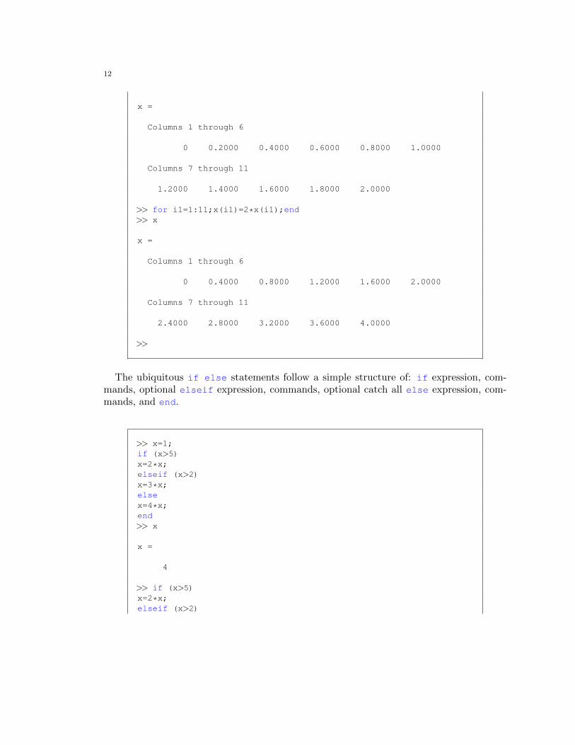
>> x=[0:.1:1];for i1=1:11x(i1)=2*x(i1);end>> x

12

x =

Columns 1 through 6

0 0.2000 0.4000 0.6000 0.8000 1.0000

Columns 7 through 11

1.2000 1.4000 1.6000 1.8000 2.0000

>> for i1=1:11;x(i1)=2*x(i1);end>> x

x =

Columns 1 through 6

0 0.4000 0.8000 1.2000 1.6000 2.0000

Columns 7 through 11

2.4000 2.8000 3.2000 3.6000 4.0000

>>

The ubiquitous if else statements follow a simple structure of: if expression, com-mands, optional elseif expression, commands, optional catch all else expression, com-mands, and end.

>> x=1;if (x>5)x=2*x;elseif (x>2)x=3*x;elsex=4*x;end>> x

x =

4

>> if (x>5)x=2*x;elseif (x>2)

13

x=3*x;elsex=4*x;end>> x

x =

12

>> if (x>5)x=2*x;elseif (x>2)x=3*x;elsex=4*x;end>> x

x =

24

>>

In true/false evaluated expressions true is the same as the number 1 and 0 representsfalse. The logical AND is represented by & and the OR is represented by —. What is thedifference between & and &&?

>> (x>2) & (x<6)

ans =

1

>> (x>2) & (x>6)

ans =

0

>> (x>2) | (x>6)

ans =

1

14

>>

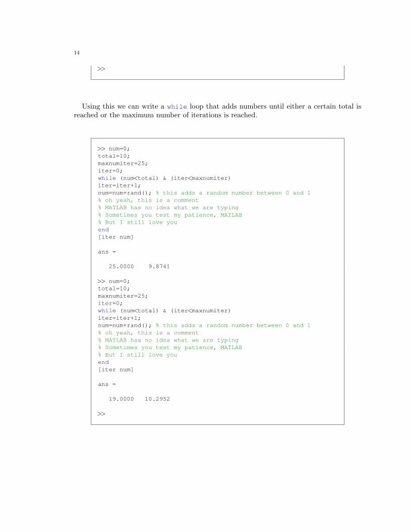
Using this we can write a while loop that adds numbers until either a certain total isreached or the maximum number of iterations is reached.

>> num=0;total=10;maxnumiter=25;iter=0;while (num<total) & (iter<maxnumiter)iter=iter+1;num=num+rand(); % this adds a random number between 0 and 1% oh yeah, this is a comment% MATLAB has no idea what we are typing% Sometimes you test my patience, MATLAB% But I still love youend[iter num]

ans =

25.0000 9.8741

>> num=0;total=10;maxnumiter=25;iter=0;while (num<total) & (iter<maxnumiter)iter=iter+1;num=num+rand(); % this adds a random number between 0 and 1% oh yeah, this is a comment% MATLAB has no idea what we are typing% Sometimes you test my patience, MATLAB% But I still love youend[iter num]

ans =

19.0000 10.2952

>>

15

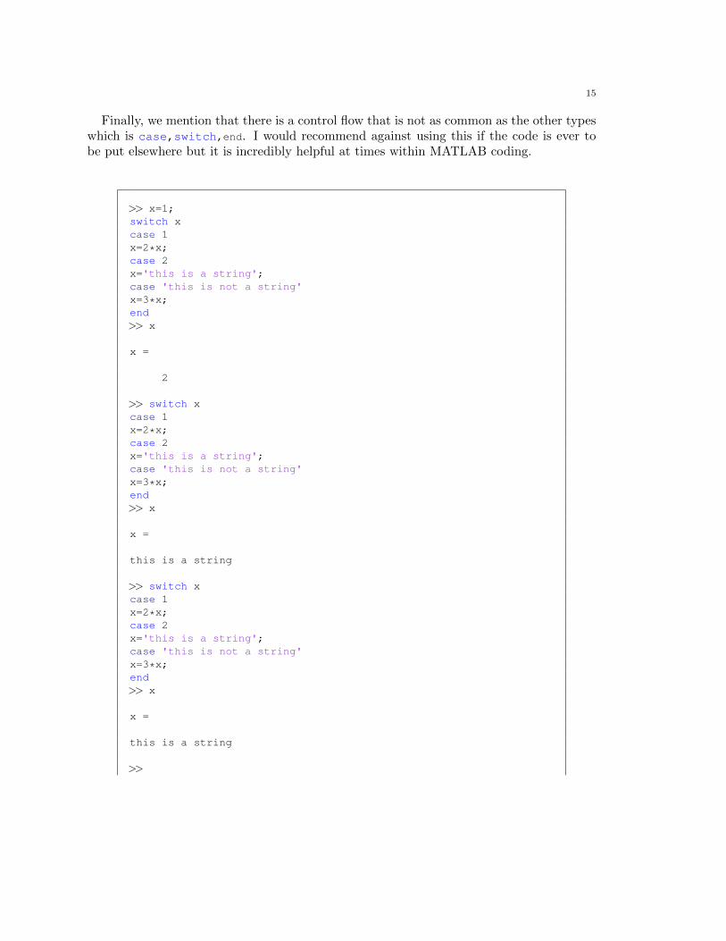
Finally, we mention that there is a control flow that is not as common as the other typeswhich is case,switch,end. I would recommend against using this if the code is ever tobe put elsewhere but it is incredibly helpful at times within MATLAB coding.

>> x=1;switch xcase 1x=2*x;case 2x='this is a string';case 'this is not a string'x=3*x;end>> x

x =

2

>> switch xcase 1x=2*x;case 2x='this is a string';case 'this is not a string'x=3*x;end>> x

x =

this is a string

>> switch xcase 1x=2*x;case 2x='this is a string';case 'this is not a string'x=3*x;end>> x

x =

this is a string

>>

16

For more information about any of these, use the help feature or similarly use doc whichbrings up a window of MATLAB documentation. So typing doc case brings up helpfulinformation about case. If your code is risky and takes chances which may result in errorsdoc try is something worthy reading.

Visualizing data, plotting

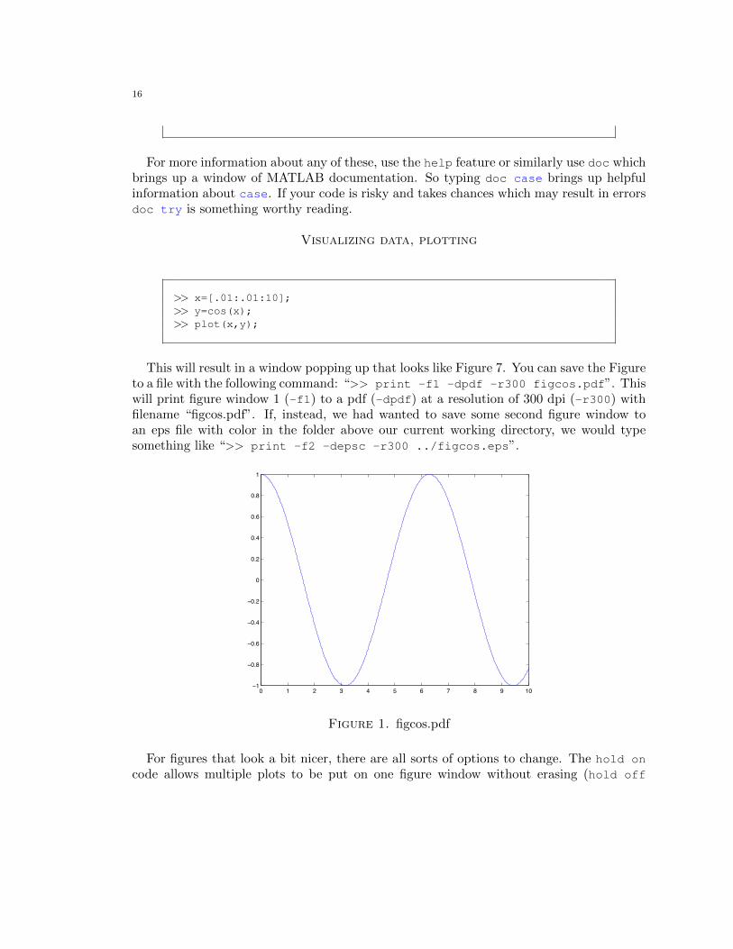
>> x=[.01:.01:10];>> y=cos(x);>> plot(x,y);

This will result in a window popping up that looks like Figure 7. You can save the Figureto a file with the following command: “>> print -f1 -dpdf -r300 figcos.pdf”. Thiswill print figure window 1 (-f1) to a pdf (-dpdf) at a resolution of 300 dpi (-r300) withfilename “figcos.pdf”. If, instead, we had wanted to save some second figure window toan eps file with color in the folder above our current working directory, we would typesomething like “>> print -f2 -depsc -r300 ../figcos.eps”.

0 1 2 3 4 5 6 7 8 9 10−1

−0.8

−0.6

−0.4

−0.2

0

0.2

0.4

0.6

0.8

1

Figure 1. figcos.pdf

For figures that look a bit nicer, there are all sorts of options to change. The hold oncode allows multiple plots to be put on one figure window without erasing (hold off

17

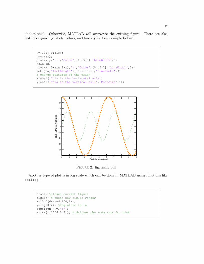
undoes this). Otherwise, MATLAB will overwrite the existing figure. There are alsofeatures regarding labels, colors, and line styles. See example below:

x=[.01:.01:10];y=cos(x);plot(x,y,'--','Color',[1 .5 0],'LineWidth',5);hold on;plot(x,.5*sin(2*x),':','Color',[0 .5 0],'LineWidth',3);set(gca,'TickLength',[.025 .025],'LineWidth',3)% change features of the graphxlabel('This is the horizontal axis')ylabel('This is the vertical axis','FontSize',14)

0 1 2 3 4 5 6 7 8 9 10−1

−0.8

−0.6

−0.4

−0.2

0

0.2

0.4

0.6

0.8

1

This is the horizontal axis

This

is th

e ve

rtica

l axi

s

Figure 2. figcosadv.pdf

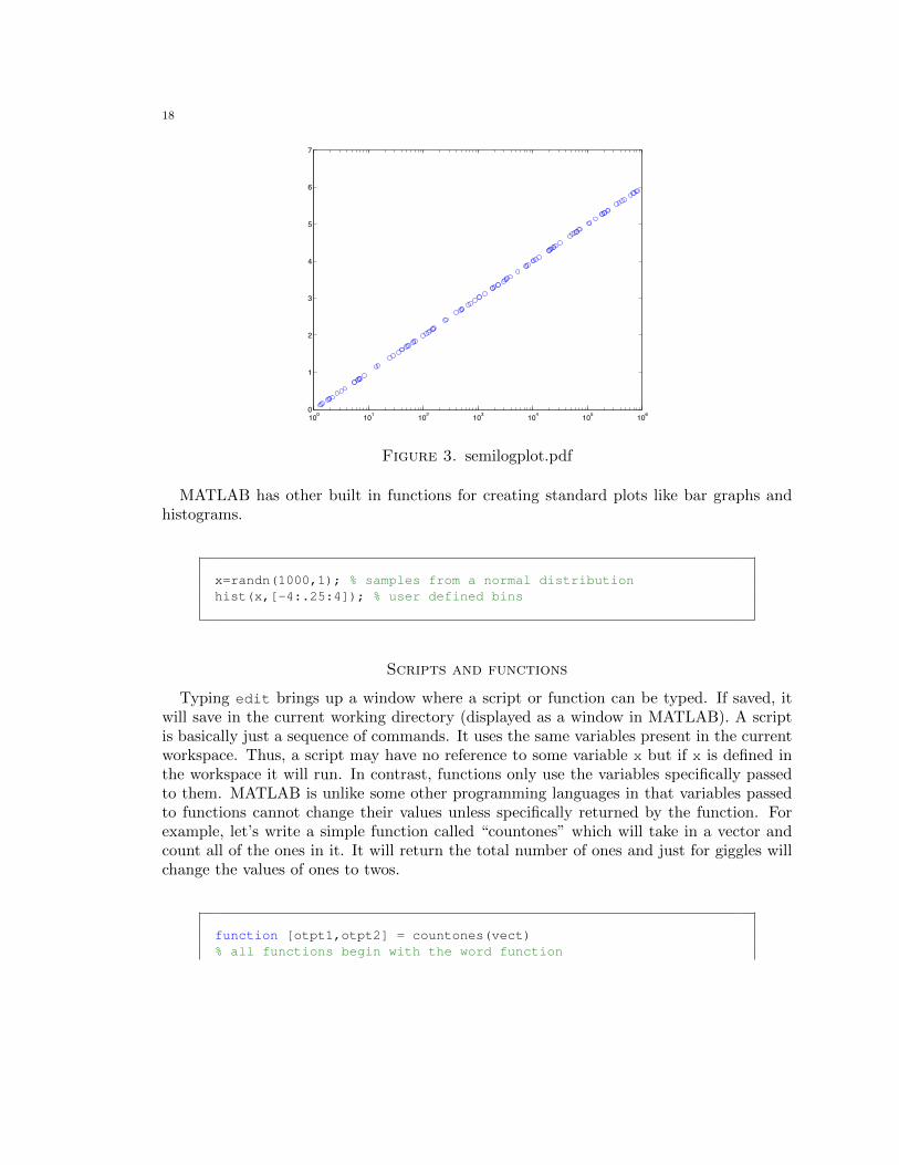
Another type of plot is in log scale which can be done in MATLAB using functions likesemilogx.

close; %closes current figurefigure; % opens new figure windowx=10.ˆ(6*rand(100,1));y=log10(x); %log alone is lnsemilogx(x,y,'o');axis([1 10ˆ6 0 7]); % defines the zoom axis for plot

18

100 101 102 103 104 105 1060

1

2

3

4

5

6

7

Figure 3. semilogplot.pdf

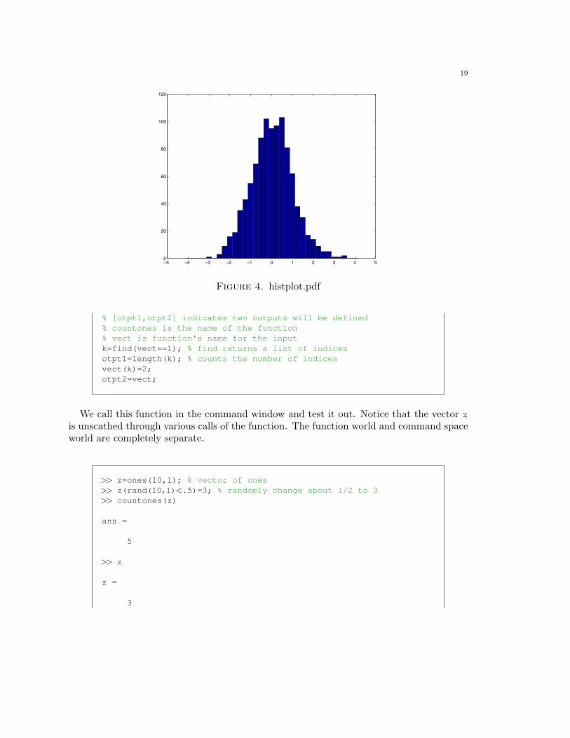
MATLAB has other built in functions for creating standard plots like bar graphs andhistograms.

x=randn(1000,1); % samples from a normal distributionhist(x,[-4:.25:4]); % user defined bins

Scripts and functions

Typing edit brings up a window where a script or function can be typed. If saved, itwill save in the current working directory (displayed as a window in MATLAB). A scriptis basically just a sequence of commands. It uses the same variables present in the currentworkspace. Thus, a script may have no reference to some variable x but if x is defined inthe workspace it will run. In contrast, functions only use the variables specifically passedto them. MATLAB is unlike some other programming languages in that variables passedto functions cannot change their values unless specifically returned by the function. Forexample, let’s write a simple function called “countones” which will take in a vector andcount all of the ones in it. It will return the total number of ones and just for giggles willchange the values of ones to twos.

function [otpt1,otpt2] = countones(vect)% all functions begin with the word function

19

−5 −4 −3 −2 −1 0 1 2 3 4 50

20

40

60

80

100

120

Figure 4. histplot.pdf

% [otpt1,otpt2] indicates two outputs will be defined% countones is the name of the function% vect is function's name for the inputk=find(vect==1); % find returns a list of indicesotpt1=length(k); % counts the number of indicesvect(k)=2;otpt2=vect;

We call this function in the command window and test it out. Notice that the vector zis unscathed through various calls of the function. The function world and command spaceworld are completely separate.

>> z=ones(10,1); % vector of ones>> z(rand(10,1)<.5)=3; % randomly change about 1/2 to 3>> countones(z)

ans =

5

>> z

z =

3

20

113313311

>> a=countones(z)

a =

5

>> z

z =

3113313311

>> a,b=countones(z) % this fails because we need brackets

a =

5

b =

5

>> [a,b]=countones(z) % this works

a =

5

b =

21

3223323322

>> z

z =

3113313311

>>

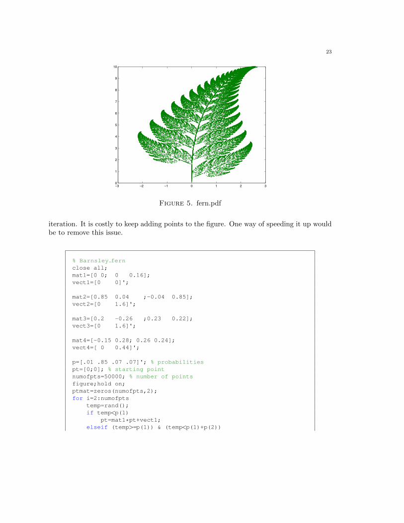
An example with ferns

Here, we show an example of MATLAB code designed to generate a Barnsley fern. Webegin with a point in the x,y coordinate system. We then apply 1 of 4 transformationsto this point. We plot that point and then choose another transformation. While thesetransformations are chosen randomly they are not equally likely. The details are below:

(1) Transformation 1 chosen 1% of the time:

xt+1 = 0xt + 0yt + 0

yt+1 = 0xt + 0.16yt + 0

(2) Transformation 2 chosen 85% of the time:

xt+1 = 0.85xt + 0.04yt + 0

yt+1 = −0.04xt + 0.85yt + 1.6

22

(3) Transformation 3 chosen 7% of the time:

xt+1 = 0.20xt +−0.26yt + 0

yt+1 = 0.23xt + 0.22yt + 1.6

(4) Transformation 4 chosen 7% of the time:

xt+1 = −0.15xt + 0.28yt + 0

yt+1 = 0.26xt + 0.24yt + 0.44

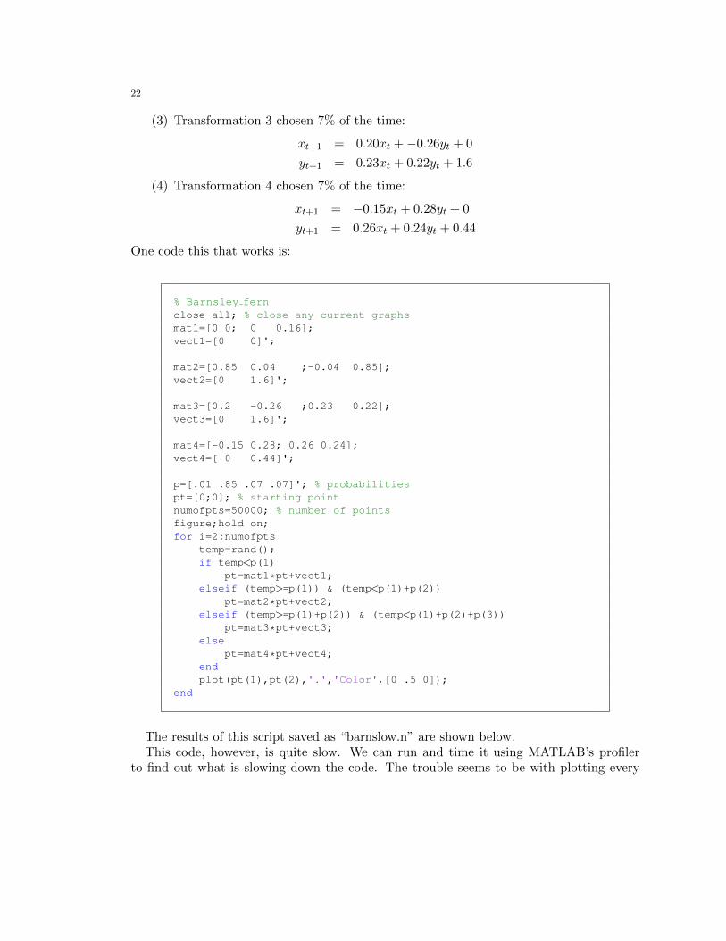
One code this that works is:

% Barnsley fernclose all; % close any current graphsmat1=[0 0; 0 0.16];vect1=[0 0]';

mat2=[0.85 0.04 ;-0.04 0.85];vect2=[0 1.6]';

mat3=[0.2 -0.26 ;0.23 0.22];vect3=[0 1.6]';

mat4=[-0.15 0.28; 0.26 0.24];vect4=[ 0 0.44]';

p=[.01 .85 .07 .07]'; % probabilitiespt=[0;0]; % starting pointnumofpts=50000; % number of pointsfigure;hold on;for i=2:numofpts

temp=rand();if temp<p(1)

pt=mat1*pt+vect1;elseif (temp>=p(1)) & (temp<p(1)+p(2))

pt=mat2*pt+vect2;elseif (temp>=p(1)+p(2)) & (temp<p(1)+p(2)+p(3))

pt=mat3*pt+vect3;else

pt=mat4*pt+vect4;endplot(pt(1),pt(2),'.','Color',[0 .5 0]);

end

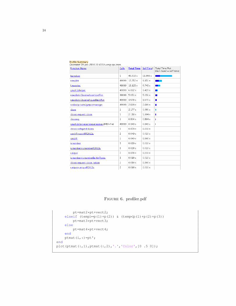
The results of this script saved as “barnslow.n” are shown below.This code, however, is quite slow. We can run and time it using MATLAB’s profiler

to find out what is slowing down the code. The trouble seems to be with plotting every

23

−3 −2 −1 0 1 2 30

1

2

3

4

5

6

7

8

9

10

Figure 5. fern.pdf

iteration. It is costly to keep adding points to the figure. One way of speeding it up wouldbe to remove this issue.

% Barnsley fernclose all;mat1=[0 0; 0 0.16];vect1=[0 0]';

mat2=[0.85 0.04 ;-0.04 0.85];vect2=[0 1.6]';

mat3=[0.2 -0.26 ;0.23 0.22];vect3=[0 1.6]';

mat4=[-0.15 0.28; 0.26 0.24];vect4=[ 0 0.44]';

p=[.01 .85 .07 .07]'; % probabilitiespt=[0;0]; % starting pointnumofpts=50000; % number of pointsfigure;hold on;ptmat=zeros(numofpts,2);for i=2:numofpts

temp=rand();if temp<p(1)

pt=mat1*pt+vect1;elseif (temp>=p(1)) & (temp<p(1)+p(2))

24

Figure 6. profiler.pdf

pt=mat2*pt+vect2;elseif (temp>=p(1)+p(2)) & (temp<p(1)+p(2)+p(3))

pt=mat3*pt+vect3;else

pt=mat4*pt+vect4;endptmat(i,:)=pt';

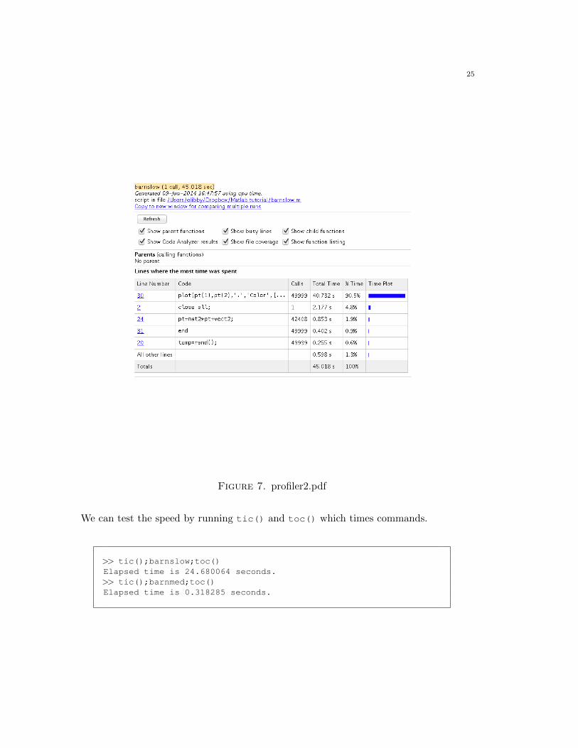
endplot(ptmat(:,1),ptmat(:,2),'.','Color',[0 .5 0]);

25

Figure 7. profiler2.pdf

We can test the speed by running tic() and toc() which times commands.

>> tic();barnslow;toc()Elapsed time is 24.680064 seconds.>> tic();barnmed;toc()Elapsed time is 0.318285 seconds.

26

Another way of coding that can show smaller gains in speed is shown below.

% Barnsley fernclose all;mat{1}=[0 0; 0 0.16]; % this is a cell arrayvect{1}=[0 0]';mat{2}=[0.85 0.04 ;-0.04 0.85];vect{2}=[0 1.6]';mat{3}=[0.2 -0.26 ;0.23 0.22];vect{3}=[0 1.6]';mat{4}=[-0.15 0.28; 0.26 0.24];vect{4}=[ 0 0.44]';p=cumsum([0 .01 .85 .07 .07]'); % probabilitiesnumofpts=50000; % number of pointsptmat=zeros(2,numofpts);inds=rand(numofpts,1);inds(inds<p(2))=1;inds(inds<p(3))=2;inds(inds<p(4))=3;inds(inds<p(5))=4;for i=2:numofpts

ptmat(:,i)=mat{inds(i)}*ptmat(:,i-1)+vect{inds(i)};endplot(ptmat(1,:),ptmat(2,:),'.','Color',[0 .5 0]);

An Example with ODE’s

Let’s imagine that we have a set of differential equations that we would like to solve.

dx

dt= 0.750x− 0.100xy

dy

dt= 0.050yx− 0.010y − 0.025yz

dz

dt= 0.025zy − 0.010z

MATLAB has several built-in functions for solving such a set of ordinary differential equa-tions. For help look up ode45. The first and last parts are particularly important.

>> help ode45ode45 Solve non-stiff differential equations, medium order method.

[TOUT,YOUT] = ode45(ODEFUN,TSPAN,Y0) with TSPAN = [T0 TFINAL]integrates the system of differential equations y' = f(t,y)from time T0 to TFINAL with initial conditions Y0.

27

ODEFUN is a function handle. For a scalar T and a vector Y,ODEFUN(T,Y) must return a column vector corresponding to f(t,y).Each row in the solution array YOUT corresponds to a timereturned in the column vector TOUT. To obtain solutions atspecific times T0,T1,...,TFINAL (all increasing or alldecreasing), use TSPAN = [T0 T1 ... TFINAL].

SKIP A BUNCH

Example[t,y]=ode45(@vdp1,[0 20],[2 0]);plot(t,y(:,1));

solves the system y' = vdp1(t,y), using the default relativeerror tolerance 1e-3 and the default absolute tolerance of1e-6 for each component, and plots the first component ofthe solution.

Class support for inputs TSPAN, Y0, and the result ofODEFUN(T,Y): float: double, single

See also ode23, ode113, ode15s, ode23s, ode23t, ode23tb,ode15i, odeset, odeplot, odephas2, odephas3, odeprint,deval, odeexamples, rigidode, ballode, orbitode,function handle.

Reference page in Help browserdoc ode45

>>

So ode45 requires a function that takes in a scalar time t and a vector Y and returns acolumn vector of the derivative of the vector y. We write a code for this set of differentialequations and name it sampdiff.

function [vp]=sampdiff(t,v)x=v(1);y=v(2);z=v(3);dxdt=.75*x-.1*x*y;dydt= .05*y*x-.01*y-.025*y*z;dzdt= .025*z*y-.01*z;vp=[dxdt ; dydt ; dzdt];

Note that this is a function which takes in a scalar time t but does not use it becausethe differentiation equations do not explicitly incorporate time. We can then call ode45

28

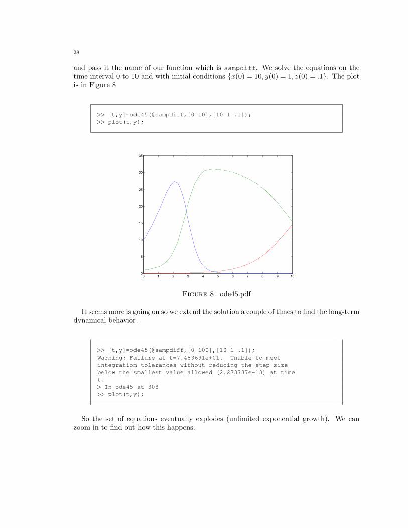
and pass it the name of our function which is sampdiff. We solve the equations on thetime interval 0 to 10 and with initial conditions {x(0) = 10, y(0) = 1, z(0) = .1}. The plotis in Figure 8

>> [t,y]=ode45(@sampdiff,[0 10],[10 1 .1]);>> plot(t,y);

0 1 2 3 4 5 6 7 8 9 100

5

10

15

20

25

30

35

Figure 8. ode45.pdf

It seems more is going on so we extend the solution a couple of times to find the long-termdynamical behavior.

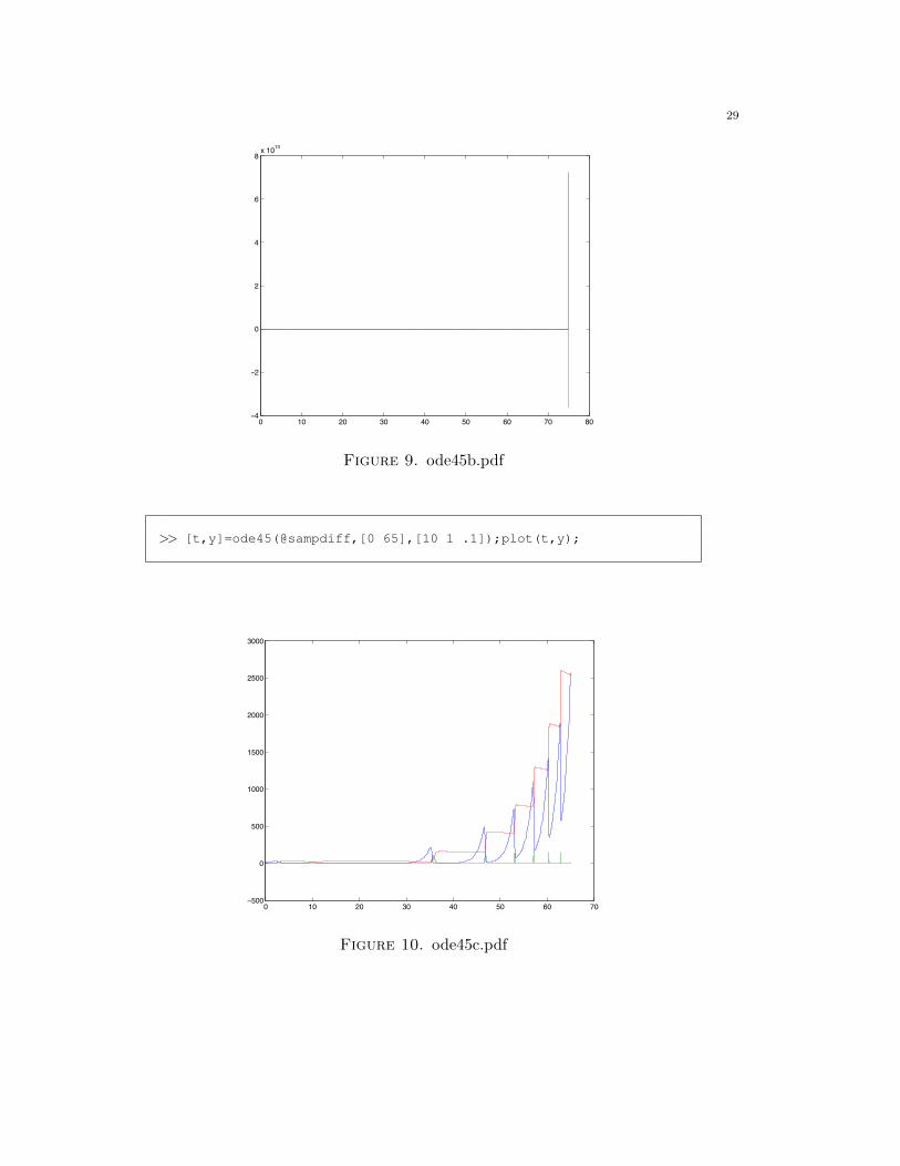
>> [t,y]=ode45(@sampdiff,[0 100],[10 1 .1]);Warning: Failure at t=7.483691e+01. Unable to meetintegration tolerances without reducing the step sizebelow the smallest value allowed (2.273737e-13) at timet.> In ode45 at 308>> plot(t,y);

So the set of equations eventually explodes (unlimited exponential growth). We canzoom in to find out how this happens.

29

0 10 20 30 40 50 60 70 80−4

−2

0

2

4

6

8x 1013

Figure 9. ode45b.pdf

>> [t,y]=ode45(@sampdiff,[0 65],[10 1 .1]);plot(t,y);

0 10 20 30 40 50 60 70−500

0

500

1000

1500

2000

2500

3000

Figure 10. ode45c.pdf

30

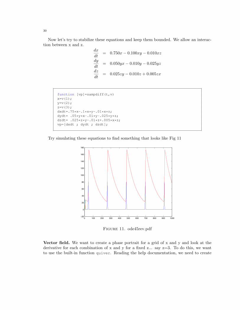
Now let’s try to stabilize these equations and keep them bounded. We allow an interac-tion between x and z.

dx

dt= 0.750x− 0.100xy − 0.010xz

dy

dt= 0.050yx− 0.010y − 0.025yz

dz

dt= 0.025zy − 0.010z + 0.005zx

function [vp]=sampdiff(t,v)x=v(1);y=v(2);z=v(3);dxdt=.75*x-.1*x*y-.01*x*z;dydt= .05*y*x-.01*y-.025*y*z;dzdt= .025*z*y-.01*z+.005*x*z;vp=[dxdt ; dydt ; dzdt];

Try simulating these equations to find something that looks like Fig 11

0 100 200 300 400 500 600 700 800 900 1000−20

0

20

40

60

80

100

120

140

160

180

Figure 11. ode45rev.pdf

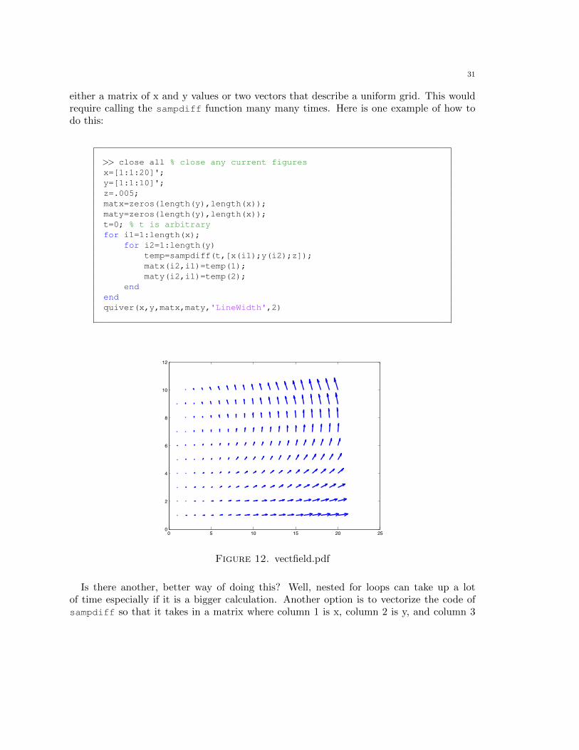
Vector field. We want to create a phase portrait for a grid of x and y and look at thederivative for each combination of x and y for a fixed z... say z=3. To do this, we wantto use the built-in function quiver. Reading the help documentation, we need to create

31

either a matrix of x and y values or two vectors that describe a uniform grid. This wouldrequire calling the sampdiff function many many times. Here is one example of how todo this:

>> close all % close any current figuresx=[1:1:20]';y=[1:1:10]';z=.005;matx=zeros(length(y),length(x));maty=zeros(length(y),length(x));t=0; % t is arbitraryfor i1=1:length(x);

for i2=1:length(y)temp=sampdiff(t,[x(i1);y(i2);z]);matx(i2,i1)=temp(1);maty(i2,i1)=temp(2);

endendquiver(x,y,matx,maty,'LineWidth',2)

0 5 10 15 20 250

2

4

6

8

10

12

Figure 12. vectfield.pdf

Is there another, better way of doing this? Well, nested for loops can take up a lotof time especially if it is a bigger calculation. Another option is to vectorize the code ofsampdiff so that it takes in a matrix where column 1 is x, column 2 is y, and column 3

32

is z and returns a matrix of the corresponding derivatives. That way we only need to callsampdiff once. We also rename it samdiffv to avoid confusion.

function [vp]=sampdiffv(t,v)x=v(:,1);y=v(:,2);z=v(:,3);dxdt=.75*x-.1*x.*y-.01*x.*z;dydt= .05*y.*x-.01*y-.025*y.*z;dzdt= .025*z.*y-.01*z+.005*x.*z;vp=[dxdt dydt dzdt];

We then need to give it proper input which is a single matrix of x,y,and z which coversall possible combinations of x and y. This is an example of how to do this.

>> close all % close any current figuresx=[1:1:20];y=[1:1:10];z=.005;t=0;tot=length(x)*length(y);[x2,y2]=meshgrid(x,y);v=[reshape(x2,tot,1) reshape(y2,tot,1) z*ones(tot,1)];vp=sampdiffv(t,v);quiver(v(:,1),v(:,2),vp(:,1),vp(:,2),'LineWidth',2)

Coding Tips

Where the heck is my Figure? MATLAB will only show a Figure if it is newly created.Any additions to an existing Figure will not bring the window forward. Instead of huntingfor the figure, simply type shg to show graph.

Faster typing. The tab key will autocomplete commands using variables from the Workspaceand previous commands typed. This is particularly helpful if your commands or variablenames are long and involved, “all of the stuff I ever needed is in this vector”. Alterna-tively, using the up arrow key will scroll through previous commands.

Common error messages

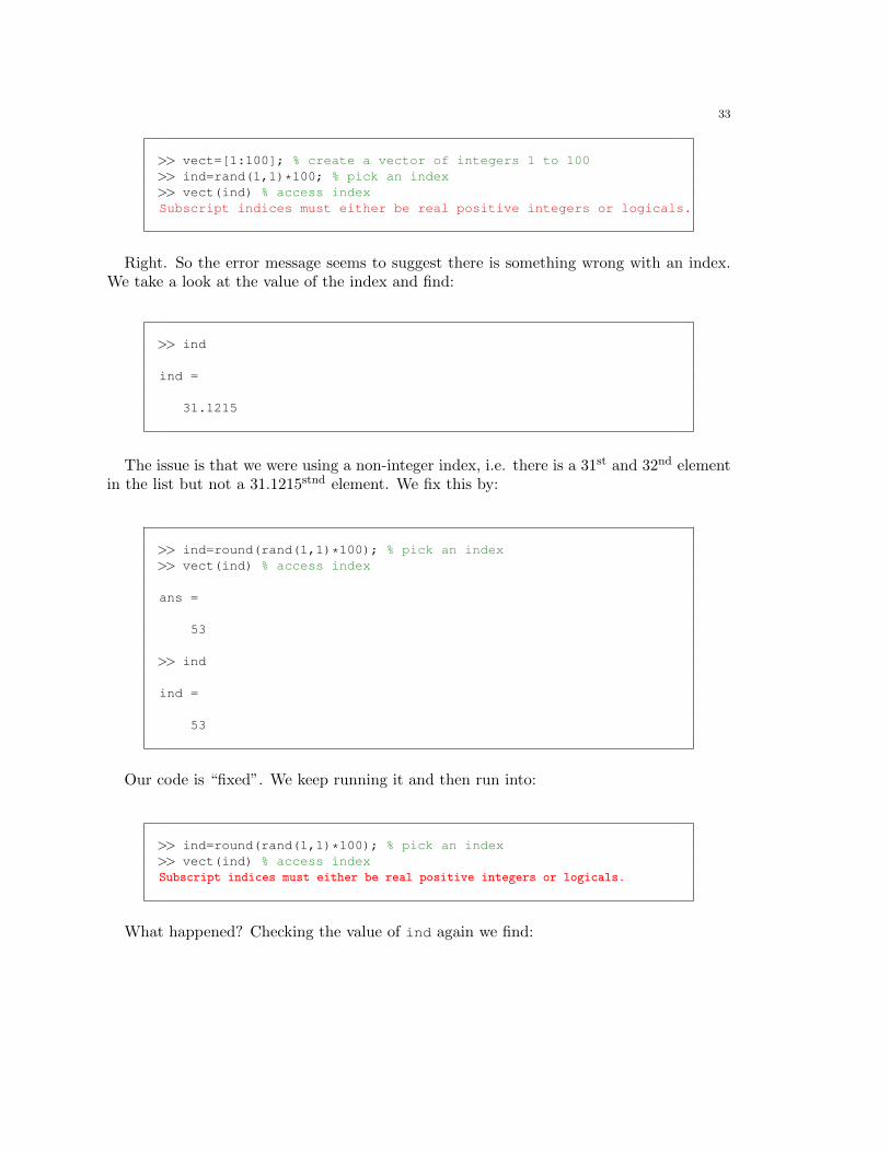
Let’s try a simple task of drawing a random sample from a vector.

33

>> vect=[1:100]; % create a vector of integers 1 to 100>> ind=rand(1,1)*100; % pick an index>> vect(ind) % access indexSubscript indices must either be real positive integers or logicals.

Right. So the error message seems to suggest there is something wrong with an index.We take a look at the value of the index and find:

>> ind

ind =

31.1215

The issue is that we were using a non-integer index, i.e. there is a 31st and 32nd elementin the list but not a 31.1215stnd element. We fix this by:

>> ind=round(rand(1,1)*100); % pick an index>> vect(ind) % access index

ans =

53

>> ind

ind =

53

Our code is “fixed”. We keep running it and then run into:

>> ind=round(rand(1,1)*100); % pick an index>> vect(ind) % access indexSubscript indices must either be real positive integers or logicals.

What happened? Checking the value of ind again we find:

34

>> ind

ind =

0

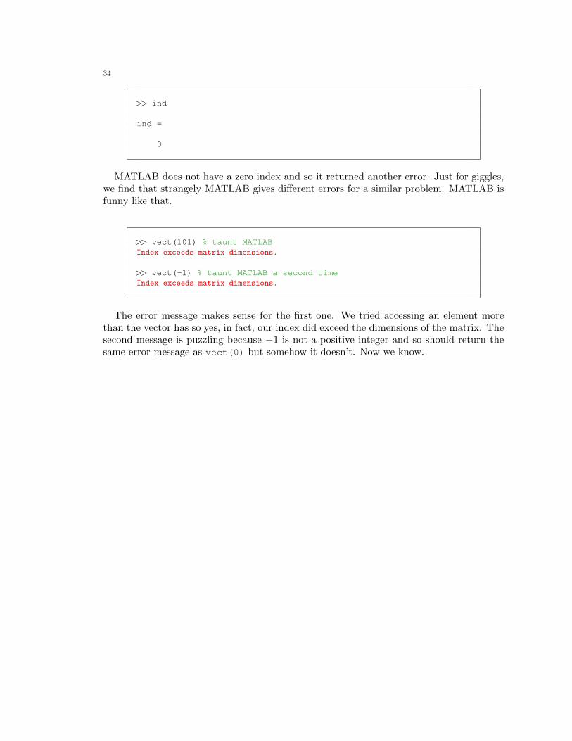
MATLAB does not have a zero index and so it returned another error. Just for giggles,we find that strangely MATLAB gives different errors for a similar problem. MATLAB isfunny like that.

>> vect(101) % taunt MATLABIndex exceeds matrix dimensions.

>> vect(-1) % taunt MATLAB a second timeIndex exceeds matrix dimensions.

The error message makes sense for the first one. We tried accessing an element morethan the vector has so yes, in fact, our index did exceed the dimensions of the matrix. Thesecond message is puzzling because −1 is not a positive integer and so should return thesame error message as vect(0) but somehow it doesn’t. Now we know.

35

Coding challenges

Binomial code. We want a function that takes in two variables: the sample size N andthe probability p of being chosen and returns y, the number chosen– effectively samplingfrom a binomial distribution. Imagine that N is very large N, say 106, and p is small, saysomewhere between 10−5 and .5. There are many ways of doing this code but here speedis of the utmost importance as this code will be sampled potentially millions of times.Write as fast a code as you can that still accurately sample from a binomial distribution.Note, MATLAB has a built in command called binornd that performs this task. Canyou determine what algorithm binornd based on clock performance alone? Can you beatbinornd?

Neutral sequence evolution. There is a population of organisms who each contain a100 base pair piece of DNA code. We are interested in the neutral evolution of this codeover time. The population goes through expansions and contractions so that it starts at106 and then goes through a growth phase of 10 generations of reproduction (growing bya factor of 210) to ≈ 109. Of this population 106 are randomly selected and the processcontinues. The DNA code of each organism is identical at the starting point and is avector of 100 entries between 1 and 4 (for A,C,G,T). Each base pair has a probability µ ofmutating into another base pair when the organism reproduces. Write a MATLAB codethat tracks the evolution of the DNA code of these organisms.

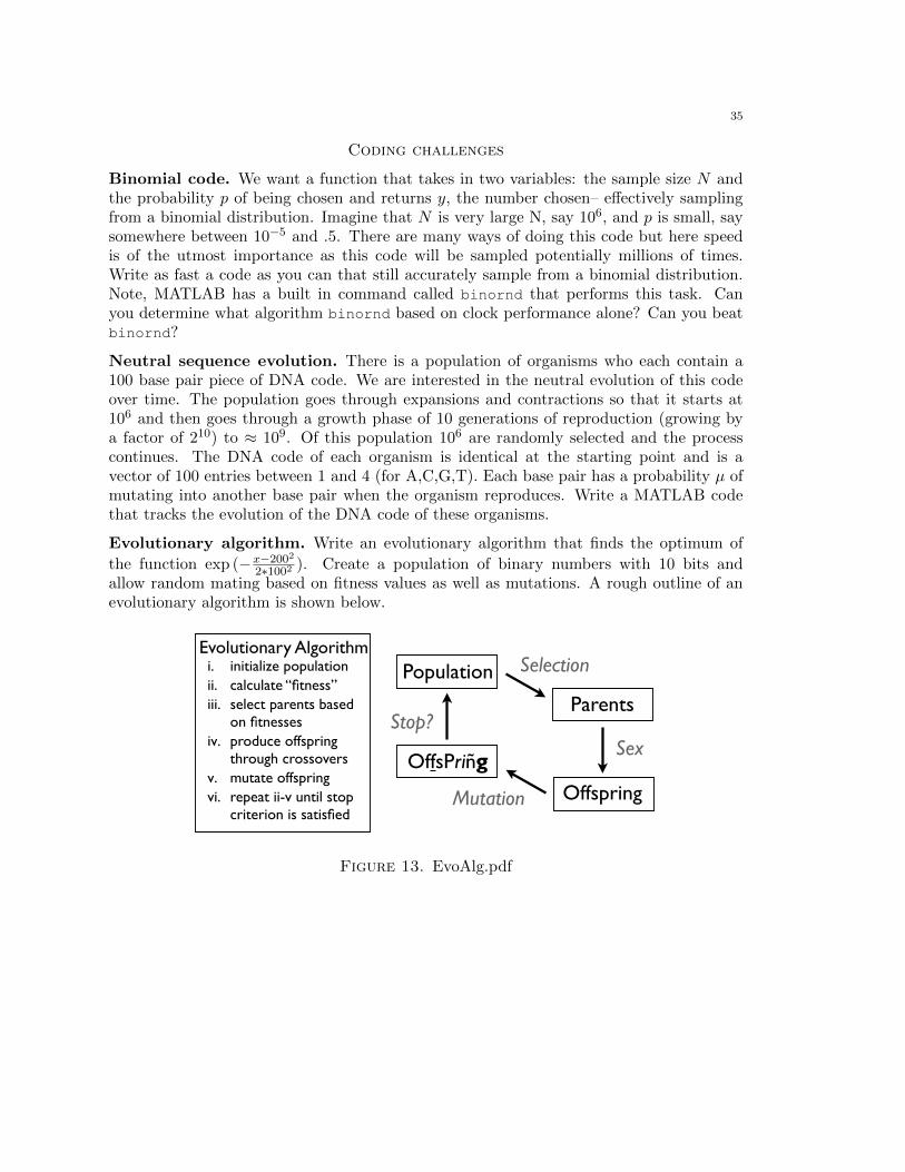
Evolutionary algorithm. Write an evolutionary algorithm that finds the optimum of

the function exp (−x−2002

2∗1002 ). Create a population of binary numbers with 10 bits andallow random mating based on fitness values as well as mutations. A rough outline of anevolutionary algorithm is shown below.

i. initialize populationii. calculate “fitness” iii. select parents based

on fitnessesiv. produce offspring

through crossoversv. mutate offspringvi. repeat ii-v until stop

criterion is satisfied

Population

Parents

Offspring

Stop?

OffsPriñg

Mutation

Selection

Sex

Evolutionary Algorithm

Figure 13. EvoAlg.pdf