NOAA Grant NA90RAH00077 National Oceanic and Atmospheric Administration

NSF Grant ATM-9015485 National Science Foundation

An Observational and Theoretical Study of Squall Line Evolution

by Erik Rasmussen

Department of Atmospheric Science Colorado State University

Fort Collins, Colorado

Steven A. Rutledge, P.1.

AN OBSERVATIONAL AND THEORETICAL STUDY

OF

SQUALL LINE EVOLUTION

by

Erik Rasmussen

Department of Atmospheric Science

Colorado State University

Fort Collins, CO 80523

Research Supported by

National Oceanic and Atmospheric Administration

under Grant NA90RAHOOO77

National Science Foundation

under Grant A TM-9015485

May 29,1992

Atmospheric Science Paper No. 500

ABSTRACT OF DISSERTATION

AN OBSERVATIONAL AND THEORETICAL STUDY OF

SQUALL LINE EVOLUTION

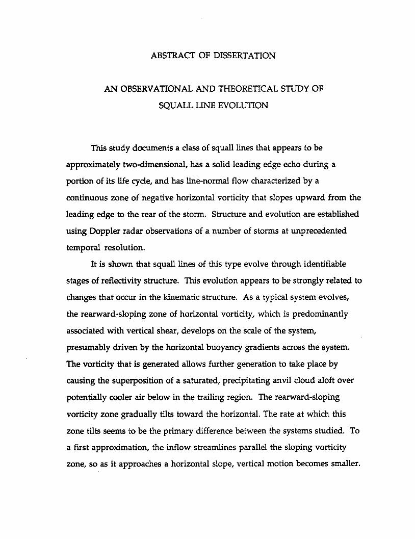
This study documents a class of squall lines that appears to be

approximately two-dimensional, has a solid leading edge echo during a

portion of its life cycle, and has line-normal flow characterized by a

continuous zone of negative horizontal vorticity that slopes upward from the

leading edge to the rear of the storm. Structure and evolution are established

using Doppler radar observations of a number of storms at unprecedented

temporal resolution.

It is shown that squall lines of this type evolve through identifiable

stages of reflectivity structure. This evolution appears to be strongly related to

changes that occur in the kinematic structure. As a typical system evolves,

the rearward-sloping zone of horizontal vorticity, which is predominantly

associated with vertical shear, develops on the scale of the system,

presumably driven by the horizontal buoyancy gradients across the system.

The vorticity that is generated allows further generation to take place by

causing the superposition of a saturated, precipitating anvil cloud aloft over

potentially cooler air below in the trailing region. The rearward-sloping

vorticity zone gradually tilts toward the horizontal. The rate at which this

zone tilts seems to be the primary difference between the systems studied. To

a first approximation, the inflow streamlines parallel the sloping vorticity

zone, so as it approaches a horizontal slope, vertical motion becomes smaller.

Eventually, convective-scale ascent ceases, giving the impression that the gust

front has surged out ahead of the precipitation.

To gain understanding of the dynamics of this class of squall lines, this

study explores the role of horizontal vorticity, and the means through which

the environment influences the rate of tilting and hence the time scale of

evolution. The observed generation of vorticity in six systems is discussed

and compared to earlier theories for squall line longevity. Motivated by these

observations, a new theory is developed which attempts to explain squall line

evolution, and the possibility of steadiness, as a function of an environment

that has both upper and lower shear regions. Predictions based on the theory

are compared to the new observations, as well as other observed and

numerically simulated squall lines.

Erik Nels Rasmussen Atmospheric Science Department Colorado State University Fort Collins, CO 80523 Spring 1992

ACKNOWLEDGEMENTS

I wish to thank my advisor, Dr. Steven Rutledge, for his support,

encouragement, and helpful discussions. I gratefully acknowledge the

support provided by the National Severe Storms Laboratory, particularly Drs.

Robert Maddox and Charles Doswell nI, who encouraged me to pursue this

degree.

The patient support of Lisa Rasmussen, and the friendship of her

family have been invaluable. I also wish to thank my parents for many years

of encouragement.

Finally, the support and friendship of Mike Smith and Dan Bowman at

WeatherData, Inc., without which the pursuit this degree would have been

much more difficult, are acknowledged with much gratitude.

TABLE OF CONTENTS

Chapter Page

1. Introduction 1

2. Observational data and methods 9 a. Data and cases studied 10 b. Analysis methods 11

3. Observations 14 a. Formative stage 16 b. Intensifying stage 16 c. Mature stage 19 d. Dissipating stage 23 e. The sloping vorticity zone 26 f. Vorticity dynamics near the leading edge 29

4. A theory for the role of the environment in evolution 32 a. Theories based on vorticity budgets: the problem of

cross-boundary transport 32 b. A simple three-region squall line 33 c. Determination of flow and vorticity fluxes 36

i. Flow as a function of inflow strength 37 ii. Flow as a function of vorticity zone strength 39 iii. Flow as a function of slope 40 iv. Total flux determined from relaxation solutions 41

d. Slope, tilt, and the predictive equation for tilting 43 e. A role of the environment in storm evolution 44 f. Comparison to observed cases 47 g. Comparison to other observations 51 h. The findings of RKW and LM interpreted

though this theory 54

5. Discussion 57

6. Conclusions 66

7. References 112

Chapter 1

Introduction

Squall lines can be defined as any non-frontal line or band of

convective activity, and the convective activity need not be continuous along

the leading edge (Hane, 1986). This study will examine a subset of this class of

convection in which the line is solid, quasi-two-dimensional, and the system

contains stratiform trailing precipitation sometime during its life cycle.

Further refinements of this definition will be made which mainly involve

the kinematic structure of the systems.

Numerous earlier studies have focused on the kinematic and

reflectivity structure of this type of precipitation system, presenting

IIsnapshots" which generally document a IImature" phase. Many findings of

the more recent studies are summarized in Rutledge (1991). Synthesis of the

observational studies has led to a conceptual model of the structure of a

mature squall line (Houze et al., 1989) illustrated in Fig. 1. Of particular

relevance here is the existence of mesoscale quasi-horizontal flow branches in

the trailing region of the storm.

As depicted in Fig. 1, a rear inflow branch slopes downward toward th~

front of the system, and is located beneath a front-to-rear branch that slopes

upward toward the rear. The strength of the storm-relative rear inflow has

been shown to vary from one system to another (Smull and Houze, 1987a).

Although this variation may be partly the result of the reference frame

chosen for the analyses, Smull and Houze showed that storms with strong

1

rear inflow also had stronger front-to-rear (FI'R) flow aloft. They also showed

that relative rear-to-front (RTF) flow was in some cases the result of

dynamical processes internal to the squall lines, and not the result of

environmental momentum being conserved as air entered the rear of the

system.

Although in previously published cases, the FI'R and RTF branches

vary in relative strength from one system to another, careful inspection

shows that there is almost always a sloping band of negative horizontal

vorticity in these systems which is largely the result of vertical shear between

the flow branches. In some storms, the vorticity zone does not extend across

the entire system, but appears only in the trailing region. In the type of squall

line investigated herein, the vorticity zone extends across the entire system.

Horizontal vorticity is defined as au aw

17=--­ik ax (1)

in a right-handed cartesian system with x normal to the squall line in the

direction of motion, and z vertical. In this study, discussion of the "vorticity

zone" refers to the region of negative horizontal vorticity which typically

extends from near the surface at the leading edge to middle or upper levels at

the rear of the system. In the conceptual model shown in Fig. I, it is found

between the sloping RTF and FI'R branches.

Examination of several previously published cases provides examples

of the nature of the vorticity zone. The 2-3 August 1981 CCOPE (Cooperative

Convective Precipitation Experiment) squall line (Schmidt and Cotton, 1989)

contained a relatively weak rear inflow jet (Fig. 2). However, it featured a

sloping region of large values of negative horizontal vorticity. This region,

situated just above the relative rear inflow zone, began near the surface at the

2

leading edge, and sloped. upward toward the rear of the storm. Similarly, a

squall line observed on 23 June 1981 during the COPI' 81 (Convection Profonde

Tropicale) experiment in tropical West Africa (Rowe, 1988) also featured the

sloping zone of vorticity (Fig. 3). In this case, it appears to be the result of

strong shear just below the upper FrR flow. An example of a system with

comparatively stronger relative rear inflow is the 10-11 June 1985 PRE­

STORM (Preliminary Regional Experiment for Stormscale Operational and

Research Meteorology) squall line (Rutledge et al., 1988), which will be

examined in further detail in this study.

In many published squall line cases, evidence can be clearly seen in the

velocity distribution of the sloping zone of negative vorticity (see, for

example Chong et al., 1987; Chalon, et al., 1988). In addition, field

observations made by the author of many squall lines in tropical northern

Australia indicate that this feature is common to most, if not all, of the squall

lines that occur there. The existence of negative vorticity in the interior part

of the squall line is a common feature of this class of squall lines, whereas the

relative strengths of the individual flow branches is not consistent from

storm to storm.

Some published cases do not show evidence of a well-defined

continuous rearward-sloping zone of negative horizontal vorticity. The

Oklahoma squallUne of 22 May 1976 has been documented using Doppler

radar analyses (Smull and Houze, 1985; Smull and Houze, 1987b) and

sounding network analyses (Ogura and Liou, 1980). Fig. 4 shows the along­

line averaged reflectivity and line-normal horizontal velocity relative to the

leading edge of this storm (from Smull and Houze, 1985). Fig. 5 shows the

larger-scale view of the same storm based on sounding analyses by Ogura and

liou (1980). In this particular squall line, a region of negative vorticity was

3

present near the leading edge (x = a in Fig. 5) in the lowest two kilometers,

and another region sloped upward from about 800 hPa to 400 hPa in the

trailing region. However, this storm did not appear to have a well-defined,

continuous rearward-sloping zone of negative vorticity. The Oklahoma squall

line of 19 May 1977 (Kessinger et al., 1987) is similar to the 22 May 1976 squall

line and also did not fit the vorticity structure of the conceptual model

described herein.

In the cases cited above, relatively little documentation was provided

on the evolution of the squall lines. One of the few studies that was able to

address evolution was that of Leary and Houze (1979). Using reflectivity data

from the GATE (GARP Atlantic Tropical Experiment), they associated the

following stages with observed reflectivity patterns:

- formative stage: line of isolated cells;

- intensifying stage: breaks fill in between cells and reflectivity

increases;

- mature stage: mesoscale precipitation features are present;

- dissipating stage: leading edge convection dissipates

The squall lines examined in this study generally followed similar

patterns in reflectivity evolution as those described by Leary and Houze.

Since there is no clear reason to depart from their terminology, these names

for the various stages will be used herein. However, the echo character and

evolution described in this study will differ significantly from those of Leary

and Houze.

This study will show evidence that certain characteristics of the squall

line, seen in both the reflectivity and kinematic structure, determine the stage

of evolution. It will be shown that squall lines undergo common patterns of

evolution. In addition, this dissertation will describe the interdependency

4

between the evolution of the reflectivity structure and the evolution of the

vorticity structure of squall lines.

Over 250 Doppler vol~e scans have been analyzed in the course of

this research, documenting numerous squall lines. For many of these cases,

data were analyzed at time intervals of about ten minutes, providing

information about squall line structure and evolution in unprecedented

detail. Ten cases were selected for detailed study based primarily on data

coverage (spatial and temporal) and the desire to span a large variety of

ambient CAPE (Convective Available Potential Energy) and environmental

wind shear conditions.

Recently, several theories have been advanced to explain the structure

and motion of squall lines and the potential for steady, long-lived systems.

Verification of these theories has awaited detailed observational and

modelling work. The validity of these the9ries is examined herein from the

perspective of the observations. Motivated by the theoretical approaches of

the earlier studies, a new theory is advanced to crudely account for variations

in the environmental vertical shear structure, and to explain evolution

without making a steadiness assumption.

Based on the results of numerical simulations, the potential for

steadiness in a squall line was examined by Rotunno et al. (1988, hereafter

referred to as RKW). RKW studied storm longevity by examining the degree

of balance (or imbalance) between vorticity transports associated with the low­

level shear in the pre-storm environment, and the generation of vorticity

5

due to the convectively-generated cold pool. The vorticity equation

appropriate to this two-dimensional, inviscid, Boussinesq problem is

where 11 is given by (1) and

d1] dB -+V·1]V=-g-at ax

B = 1- 8y + q 8 c. y

(2)

(3)

Total buoyancy is represented by B, with qc being the total condensate mixing

ratio, and 9v is the virtual potential temperature.

Several assumptions were made by RKW to permit the integration of

this vorticity equation. First, it was assumed that an ideal condition in a long­

lived, intense squall line was a vertically-issuing, symmetric updraft above

the propagating cold pool. Furthermore, it was assumed that vorticity is only

transported across the forward boundary of the integration volume, and not

the rear boundary. By assuming a steady flow, RKW demonstrated that a

balance between the cold-pool generation of vorticity and the transport of the

low-level ambient vorticity associated with the vertical shear of the

horizontal wind in the pre-storm environment is required for steady, intense

systems. RKW focussed on the dynamiCS of the lowest few kilometers, and

did not address the effects of buoyancy gradients or transport in the regions

above.

In simulations of a West Africa squall line case from the COPT 81

experiment, Lafore and Moncrieff (1989, hereafter referred to as LM)

recognized that vorticity generation occurs on the scale of the squall line,

including the trailing stratiform region. In terms of the horizontal extent

detected by radar, this can be as broad as 100 km or more (refer to Fig. 1). They

argued that vorticity is generated by horizontal gradients of buoyancy that

6

result from thermodynamic and microphysical processes throughout the

storm, not just in the vicinity of the leading edge of the cold pool. This

argument is clearly supported by the observations of vorticity evolution

presented herein. However, LM did not address the issue of how the system­

scale vorticity structure and generation impacts the rate of evolution or

potential for steadiness.

In comments following publication of LM, Rotunno et al. (1990)

indicate that the theory of RI<W only addressed the conditions necessary for

producing vigorous, uninhibited ascent at the gust front of a squall line. They

suggested that an intense, long-lived system would be more likely when such

ascent occurs. In reply, Lafore and Moncrieff (1990) reiterated that although

the process described by RI<W is a necessary condition for an intense, long­

lived system, other factors impact "both the leading edge convection and the

global dynamics." Further, Lafore and Moncrieff (1990) stressed that the

upstream environment, in which low-level shear is measured, is itself

modified by squall lines.

Seitter and Kuo (1983) also argued that vorticity generation is a storm­

scale process, and showed the role of gravity in generating buoyancy gradients'

through the decoupling of the buoyant updraft air and the negatively buoyant

precipitation-laden air. Emanuel (1986) used linear theory to expand on this

concept and demonstrate the likely modes of propagation and orientation of

squall-line like disturbances.

It is very convenient to use vorticity arguments to describe storm

dynamics. Clearly, the buoyancy and momentum distributions lead to the

generation of pressure perturbations which also could be used to describe the

evolution of the flow. Many observational studies have focussed on the role

of these pressure perturbations. For example, Lemone (1983) documented the

7

role of lowered pressure beneath the sloping cloudy region, warmed by

condensation heating, to explain various observed accelerations. The roles of

the surface mesoscale pressure perturbations have also been explored (e.g.

Johnson and Hamilton, 1988). Modelling studies have long indicated the

importance of perturbation high pressure near the summits of updrafts in

leading to adverse vertical accelerations as well as summit divergent flow

(e.g. Schlesinger, 1975). It is important to note that the accelerations that must

occur to alter the distribution of horizontal vorticity are partially the result of

these pressure perturbations. Any or all of the following pressure features

may be associated with increasing negative vorticity in the interior of the

squall line: high pressure aloft near the leading edge, low pressure along the

underside of a sloping region of relatively warm air, and high pressure near

the surface in the area behind the convective line. However, in order to

understand the evolution of squall lines, horizontal vorticity arguments are

often simpler and do not require discussion of the actual distribution of

pressure in the storm.

Following the vorticity viewpoint and utilizing Doppler radar

observations, this study will further explore the role of buoyancy gradients·

and vorticity transport in controlling squall line evolution. Motivated by the

observational findings, a theory is presented for squall line evolution that

includes consideration of environmental shear in two layers (a "lower" and

"upper" layer in contrast to the single layer in RKW) and the storm-generated

vorticity structure.

8

Chapter 2

Observational data and methods

The focus .of this study is the evolution of the two-dimensional, line­

normal structure of squall lines. Such a focus is best suited to cases in which

the variation in flow along the convective line is small compared to that

across the line. From a dynamical viewpoint, one condition for two­

dimensionality is that the regions containing buoyancy anomalies of a given

sign be much longer than they are wide. These conditions generally exclude

those periods of squall line life cycles with structures typified by mesoscale

vortex motion, and squall lines composed of individual storms separated by

echo-weak regions, while still allowing for some cellul.ar structure to the

leading edge convection. The possibility of along-line flow is not excluded,

even if it is strong.

All of the squall lines analyzed in this research were chosen because of

their apparently high degree of two-dimensionality in order facilitate

interpretation of their dynamics from theoretical perspectives. The dynamiCS

of squall lines that satisfy two-dimensionality can be readily assessed using

single Doppler radar data, provided that data samples can be obtained normal

to the leading edge of the system. Of great importance is the availability of

data with sufficient temporal resolution to document changes in the squall

line structure. The needed temporal resolution depends somewhat on the

rate of evolution, but most of the cases selected for this study had volume

scan data at intervals of ten to fifteen minutes.

9

a. Data and cases studied

Radar data used in this research were obtained in two experiments: the

Down-Under Doppler and Electricity Experiment ("DUNDEE", Rutledge et al.,

1992) in tropical northern Australia, and the 1985 PRE-STORM experiment

(Cunning, 1986) in Kansas and Oklahoma. The radars from these

experiments used in this study were the MIT (Massachusetts Institute of

Technology) and NOAA/TOGA (National Oceanic and Atmospheric

Administration/Tropical Oceans and Global Atmosphere) radars in the

DUNDEE cases, and the NCAR (National Center for Atmospheric Research)

CP-4 radar in the PRE-STORM case. All of these radars are 5 an wavelength

Doppler radars. Further details concerning these radars can be found in the

references cited immediately above.

Table 1 summarizes the cases studied. Various data sets had certain

limitations, such as inadequate temporal resolution, failure to scan at high

elevation angles, etc. So although all ten cases were useful in determining

Table 1: List of cases analyzed.

Number of volume scans analYZed

10-11 June 1985 25 26 November 1988 21 26 January 1989 20 18 November 1989 23 5 December 1989 19 24 January 1990 9 7 February 1990, first storm 14 7 February 1990, second storm 18 7 February 1990, third storm 9 14 February 1990 29

10

Experiment

PRE-STORM DUNDEE DUNDEE DUNDEE DUNDEE DUNDEE DUNDEE DUNDEE DUNDEE DUNDEE

the general features of structure and evolution described in this study, only

seven were suitable for the detailed analyses required to evaluate vorticity

budget integrals.

b. Analysis methods

The first step in the data analysis involved editing the raw radar data to

remove non-meteorological echoes and unfold the radial velocity data. It was

assumed that the target velocity vectors were composed of purely horizontal

flow plus the hydrometeor fallspeed, so that

vr Vh = ---vttana

cosa (4)

where Vh is the horizontal velocity component, Vr is the radial (measured)

component, a is the elevation angle, and Vt is an estimated terminal velocity.

The terminal velocity was estimated using a power law relation with

different values for coefficientand exponent above and below the melting

level. The general conclusions reached herein are based largely on velocities

observed at elevation angles low enough that the cosa and Vt sensitivities

were unimportant.

In order to examine the evolution of the 2-D flow on the scale of the

squall line, reflectivity and horizontal velocity data were averaged in slabs

that extended across the squall line approximately orthogonal to the leading

edge. The slabs were usually 20 kIn wide, and the orientation and width was

held constant for the duration of the storm, even if the squall line orientation

shifted somewhat as the system propagated. Each radar data point that fell

11

within the slab was assigned to the nearest grid point, with the grid resolution

being 1000 m in the horizontal, line-normal direction, and 500 m in the

vertical.

The purpose of the slab-averaging technique was to filter the features

in the along-line direction, while retaining all features with broad line­

normal extent. Using only single Doppler radar data, it was not possible to

obtain legitimate 2-D averages over wider sections of the squall line. The

good degree of temporal continuity in the slab-averaged data suggests that the

technique is a reasoriably good method for filtering the convective scale

along-line variations. In order to ensure that the horizontal velocity

computed in the manner described above was representative of the

component in the line-normal direction, only data that fell within 12.5·

azimuth of the slab center-line were used. This requirement implied that at

ranges very close to the radar, smaller-scale, features were being retained since

a smaller along-line sample is utilized. Because of this, quantities such as

vertical velocity are interpreted with great caution when diagnosed near the

radar, because they may be representative of an individual convective cell

instead of an average over the slab width. Finally, if more than one-third of

all possible radar data points that mapped to a single slab data point had data,

the data were averaged for that point. If too few radar data estimates were

available, the slab-average value was not obtained for that grid point.

After computing slab averages, an additional smoothing step was

performed on the horizontal velocities using a Gaussian filter. This filter

retained approximately 75% of the amplitude of features with 4 kilometer

wavelengths, increasing toward 100% at longer wavelengths and filtering

more strongly at shorter wavelengths. For regions below the radar horizon of

1.5 km depth or less, horizontal velocity estimates were filled using

12

objectively analyzed estimates of du/ dz, applying the same Gaussian

weighting function to the nearby estimates of du/ dz above the radar horizon.

This technique was tested by assuring that the resulting vorticity fields had

good spatial continuity from data-rich to data-poor regions, and that as the

storms propagated into regions with different radar horizons, vorticity fields

near the ground showed good temporal continuity. The primary purpose of

filling velocities below the radar horizon was to obtain estimates of

horizontal divergence in that region for use in computing vertical velocity.

The sub-horizon velocity estimates do not have a significant impact on the

findings presented herein.

The vertical velocity was diagnosed using downward integration of the

anelastic continuity equation, with the boundary condition being w=O at the

radar echo top. A density profile appropriate for the particular geographical

region was used. Residual velocity at the bottom of each column was used to

compute the amount of divergence required over the column depth to satisfy

a lower boundary condition of w=O. This divergence was then applied, and

the integration performed again, resulting in satisfying boundary conditions

of w=O at both the echo top and ground. It was found that this technique

produced vertical velocity fields that were more uniform in time and space,

and more "realistic looking", than those produced with simple top-down

integration. Using centered finite differences, horizontal vorticity (Eq. 1) was

then computed from horizontal and vertical velocity data.

13

Chapter 3

Observations

A large number of slab-average fields have been examined in detail

(temporal resolution of 10-15 min) for ten squall line cases. These fields

include reflectivity, horizontal and vertical velocity, horizontal vorticity,

divergence, and vertical and horizontal shear. In this section, each stage of

evolution will be described in detail. These descriptions form a conceptual

model of squall line evolution that is based on thorough analysis of all ten

squall line cases, and represents a synthesis of those features that appear to be

common to all of the cases. In addition to the ten cases, numerous other

storms have been observed by the author that fit the general model presented

here. Based on the case study analysis, four distinct stages of evolution are

recognizable. Retaining the nomenclature of Leary and Houze (1979), these

are called the formative, intensifying, mature, and dissipating stages. Since

not every storm was observed in all four stages (because of limitations in

radar coverage), those cases best representing each stage will be used for

illustration in this section. A special nomenclature will be used to name the

cases consisting of the date and a suffix (F,M,S) to indicate whether the storm

was fast-evolving, moderately. evolving, or slow-evolving when subjectively

compared to the other cases in this study. For example, the case designated

7feb90M is a squall line that occurred on 7 February 1990, and was moderate in

speed of evolution compared to the other cases.

14

The data will be described in terms of storm-relative flow, with the

translation speed being that of the leading edge of the squall line during the

mature stage. This seems to be the most common way to represent squall line

flow. However, two caveats are necessary. First, squall line motion is not

generally steady in the systems examined. Rather, the systems tend to

accelerate during the intensifying stage. Second, propagation speed is not

uniform for all parts of the convective system. The leading edge propagates

the most quickly, with features further rearward propagating more slowly,

and the trailing anvil edge moving the slowest. This variance in propagation

speed is obviously required if the system is to expand rearward with time. It

is for these reasons that the squall lines discussed herein will be described

mainly in terms of vorticity, which is invariant for any choice of translation

speed.

All of the slab-average vertical cross. sections sho~ in this dissertation

are oriented so that the system is propagating from left to right. The leading

edge convection is placed near the right edge of the figures. The horizontal

distance is in kIn along the path of propagation (positive x), with the radar

situated near x=115 kIn. The orientation of the slabs is depicted in the figures .

showing the horizontal distribution of reflectivity.

Defining the four stages of evolution is done mainly to facilitate

discussion. The evolution is really a continuum of changes in the kinematic

and reflectivity structure, broadly characterized by gradual tih.'1.e flow

branches and reduction in updraft strength and echo intensity. FucuLd

discussion and illustration of the four stages can be found in Chapter 5 and

Fig. 45.

15

a. Formative stage

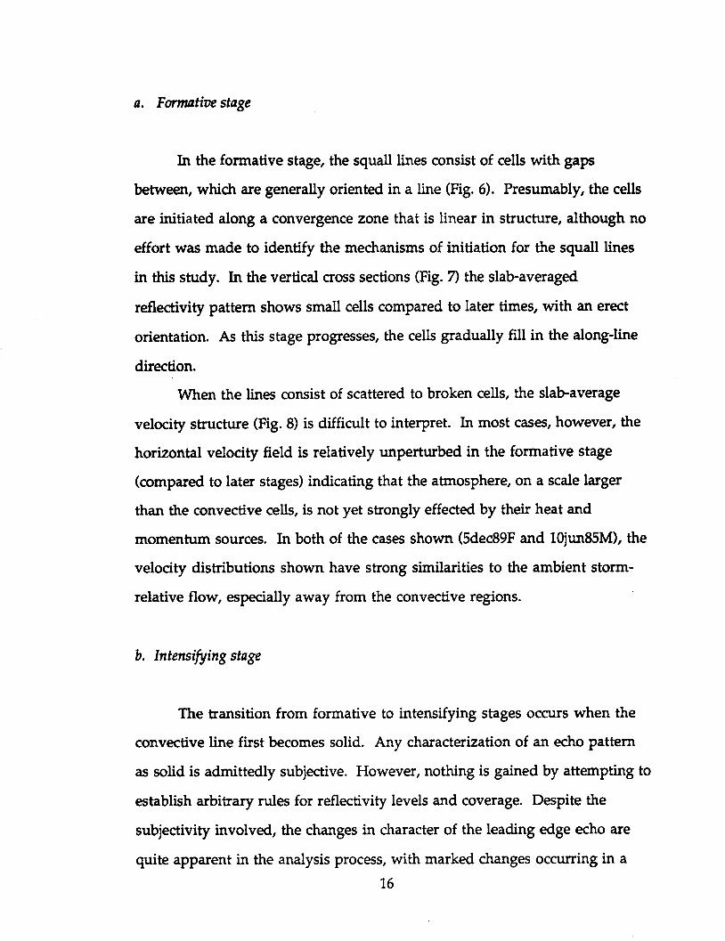
In the formative stage, the squall lines consist of cells with gaps

between, which are generally oriented in a line (Fig. 6). Presumably, the cells

are initiated along a convergence zone that is linear in structure, although no

effort was made to identify the mechanisms of initiation for the squall lines

in this study. In the vertical cross sections (Fig. 7) the slab-averaged

reflectivity pattern shows small cells compared to later times, with an erect

orientation. As this stage progresses, the cells gradually fill in the along-line

direction.

When the lines consist of scattered to broken cells, the slab-average

velocity structUre (Fig. 8) is difficult to interpret. In most cases, however, the

horizontal velocity field is relatively unperturbed in the formative stage

(compared. to later stages) indicating that the atmosphere, on a scale larger

than the convective cells, is not yet strongly effected by their heat and

momentum sources. In both of the cases shown (Sdec89F and lOjun85M), the

velocity distributions shown have strong similarities to the ambient storm­

relative flow, especially away from the convective regions.

b. Intensifying stage

The transition from formative to intensifying stages occurs when the

convective line first becomes solid. Any characterization of an echo pattern

as solid is admittedly subjective. However, nothing is gained by attempting to

establish arbitrary rules for reflectivity levels and coverage. Despite the

subjectivity involved, the changes in character of the leading edge echo are

quite apparent in the analysis process, with marked changes occurring in a

16

matter of minutes (i.e. from one volume scan to the next). Comparison of

the horizontal reflectivity distributions of the formative stage (Fig. 6) and the

intensifying stage (Fig. 9) shows the change in echo character.

The slab-averaged reflectivity (Fig. 10) shows that the cells have grown

in horizontal and vertical extent. There is a sligh t rearward tilt to the leading

edge convective cores (especially 26nov88S, 5dec89F, and 10jun85M; panels b­

d), and there is also a small area of trailing echo in some of the cases. This

trailing echo may be the remnants of earlier convective cells that have

moved rearward relative to the leading edge.

By the end of the intensifying stage, the leading edge convective cells

reach their greatest vertical extent and largest updraft speeds. Examples of the

evolution of updraft speeds, based on the 2-D calculation of vertical velocity,

are shown in Fig. 11. For each slab, vertical velocities were averaged in

regions 2 kIn deep and 5 kIn in line-normal extent. The vertical velocities

obtained with this averaging method are shown in Fig. 11. Neglecting the

higher frequency variations, broad peaks in vertical velocity of about 5-6 ms-1

occur toward the end of the intensifying stage. The peak updraft velocity then

falls off rapidly during the mature stage. This pattern is repeated among allot

the cases, and thus it is suggested that the peak vertical velocity is the clearest

indicator of the transition from intensifying to mature stages.

The observations above indicate that the intensifying stage should be

defined as the period beginning when the line becomes solid, and ending at

the time of maximum vertical .echo extent and updraft intensity in the

leading edge. This definition of the intensifying stage differs from that of

Leary and Houze which allows gaps between cells. However, the data

presented herein suggest that changes in the flow structure occur much more

rapidly after the line becomes solid. This is almost certainly associated with

17

r

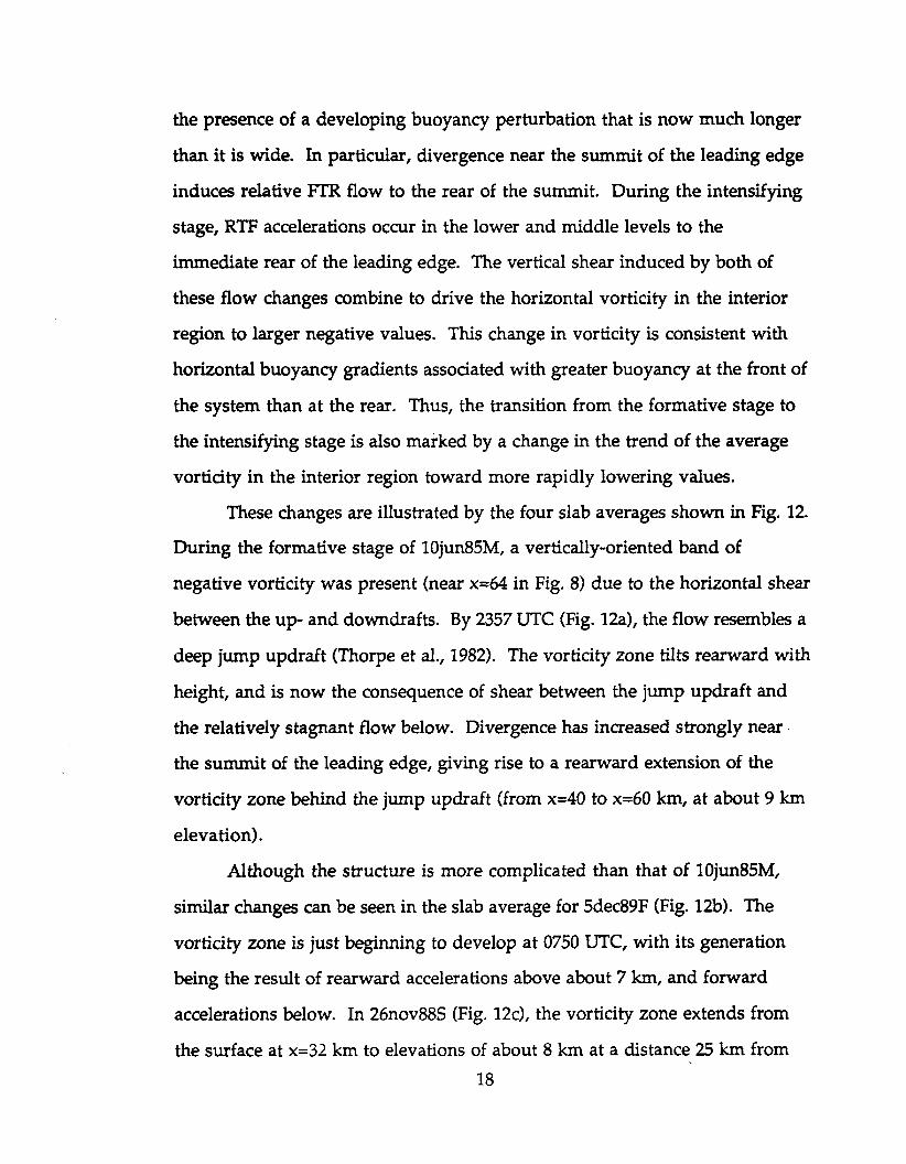
the presence of a developing buoyancy perturbation that is now much longer

than it is wide. In particular, divergence near the summit of the leading edge

induces relative FIR flow to the rear of the summit. During the intensifying

stage, RTF accelerations occur in the lower and middle levels to the

immediate rear of the leading edge. The vertical shear induced by both of

these flow changes combine to drive the horizontal vorticity in the interior

region to larger negative values. This change in vorticity is consistent with

horizontal buoyancy gradients associated with greater buoyancy at the front of

the system than at the rear. Thus, the transition from the formative stage to

the intensifying stage is also marked by a change in the trend of the average

vorticity in the interior region toward more rapidly lowering values.

These changes are illustrated by the four slab averages shown in Fig. 12.

During the formative stage of 10jun8SM, a vertically-oriented band of

negative vorticity was present (near x=64 in Fig. 8) due to the horizontal shear

between the up- and downdrafts. By 2357 UTC (Fig. 12a), the flow resembles a

deep jump updraft (Thorpe et al., 1982). The vorticity zone tilts rearward with

height, and is now the consequence of shear between the jump updraft and

the relatively stagnant flow below. Divergence has increased strongly near·

the summit of the leading edge, giving rise to a rearward extension of the

vorticity zone behind the jump updraft (from x=40 to x=60 km, at about 9 km

elevation).

Although the structure is more complicated than that of 10jun8SM,

similar changes can be seen in the slab average for Sdec89F (Fig. 12b). The

vorticity zone is just beginning to develop at 0750 UTC, with its generation

being the result of rearward accelerations above about 7 km, and forward

accelerations below. In 26nov885 (Fig. 12c), the vorticity zone extends from

the surface at x=32 km to elevations of about 8 km at a distance 25 km from

18

the leading edge. A similar slope can be seen in the vorticity pattern of

14feb90M (Fig. 12d).

Another interesting transition found in the majority of the cases is

seen in the propagation speed of the leading edge convection, shown in Fig.

13. During the formative and intensifying stages, the speed is relatively small

and less than the mean flow through the depth of the convection. It is

perhaps representative of some combination of Usteering flow" and low-level

momentum. However, at about the time of the transition between the

intensifying and mature stages, the squall line suddenly accelerates to a speed

more representative of a density current propagation speed (Charba, 1974).

The reasons for these changes in propagation speed are not clear, but it is

possible that the acceleration in the speed of the system may be associated

with the development of a low-level cold pool that propagates in a similar

fashion to a density current and forces ascent along its leading edge.

c. Mature Stage

The transition from the intensifying to the mature stage is more subtle

than the transition between the earlier stages. During the intensifying stage,

convective vigor increases as measured by peak updraft velocities, for

example. During the mature stage, the vorticity zone and attendant draft

structure gradually tilt tuward the horizontal, leading to a gradual decrease in the

updraft strength. Based on updraft speed alone, it could be argued that there

is not a "mature" stage, since the leading edge updrafts begin dissipating after

the intensifying stage. However, mesoscale ascent and vorticity generation

continue, leading to a marked increase in the horizontal extent of the system.

Thus, although leading edge vigor may wane slowly during the mature stage,

19

the system continues to grow and produce precipitation over larger areas, in

agreement with the findings of McAnelly and Cotton (1989).

During the mature stage, inflow is initially lifted near the leading edge

of the cold pool, but then continues to ascend for some distance behind the

leading edge. As tilting progresses, the streamlines become more horizontal

after passing over the gust front. The mature stage ends when these

streamlines become oriented so horizontally that the leading edge character

changes from a solid line of convection to patchy, weak, and shallow

convective cells atop the cold pool or weak stratiform ascent. This is a

difficult transition to detect, but is dynamically important since the heating

generated by convective ascent at the leading edge of the system changes from

a solid, relatively deep and strong heat source to a shallow, weak source

which may be discontinuous along the line. At the same time, heating forced

by mesoscale ascent becomes more widespread in the trailing region.

Negative vorticity continues to be generated through the mature stage.

This generation is the result of buoyancy gradients between the solid leading

edge (positive buoyancy anomaly) and a negative buoyancy anomaly toward

the rear of the system. The increasing FfR relative flow aloft increases the

transport of hydrometeors from the leading region into the trailing region

aloft, causing the echo and precipitation area to expand rearward. Increasing

RTF relative flow beneath this expanding anvil cloud, or often simply the

expansion of the anvil over relatively stagnant lower-level air, can lead to

cooling from evaporation and sublimation. Cooling owing to melting also

occurs as ice hydrometeors fall through the melting level. Observations of

the location and slope of the vorticity zone in the squall lines in this study

indicate that the negative buoyancy anomaly is better characterized as a

20

sloping region, presumably following the underside of the anvil cloud in the

trailing region, rather than a "cold pool" at the ground.

Thus the mesoscale flow structure is characterized by negative

vorticity, with relative rearward-directed flow above weaker flow in the same

direction, or relative forward-directed flow. As the vorticity increases, the

relative flows increase, and ice is transported to ever greater distances to the

rear of the leading edge. This in turn causes the continual spreading of the

negative buoyancy anomaly further toward the rear aloft. As long as these

buoyancy anomalies persist, the negative vorticity can increase. One effect of

this feedback process is that the overall system increases in horizontal scale. .

This is because the generation of vorticity in the storm is manifested as

increasingly-sheared horizontal flow, which allows the precipitation­

generating anvil cloud to move rearward relative to the leading edge source

region.

The general structure of all of these squall lines is one of a jump

updraft (Thorpe et ai. 1982), with the overturning updraft branch occasionally

observed. The inflowing air turns upward in the jump updraft and then

turns rearward at higher elevations, with storm-relative streamlines parallel'

to the vorticity zone (to a first approximation), as shown in Fig. 14. The more

erect portion of the jump updraft comprises the convective-scale ascent, and

since the streamlines are approximately parallel to the vorticity zone, the

slight slope of the trailing portion indicates mesoscale ascent. As time

progresses during the mature stage, the vorticity zone becomes less sloped,

tending toward a more horizontal orientation. Thus the ascent becomes

weaker and spread over a wider band. This agrees with the observation that

leading edge echoes become broader and weJ.ker with time. The dynamics

and implications of this tilting process are discussed in detail in Chapter 4.

21

Data from cases 10jun85M, 14feb90M, 26nov88S, and 26jan89S are used

to illustrate various aspects of the mature stage. The low-level, horizontal

distribution of reflectivity is shown in Fig. 15. Several marked changes are

apparent when this stage is compared to the intensifying stage (Fig. 9). First,

the leading edge convection remains relatively intense in the low levels, but

the convective cores have widened rearward. Because of the more horizontal

orientation of the streamlines described above, the leading edge ascent, and

thus precipitation generation, is now spread over a wider zone. Three storms

featured transition zones (all but 14feb90M). In all cases, stratiform

precipitation had become quite widespread in the mature stage. This is a

consequence of the strong storm-generated shear and the mechanism of

upscale-growth described above. Clearly, this increase in horizontal scale is

the major difference between the intensifying and mature stage.

The slab-average vertical reflectivity structure is shown in Fig. 16. It

can be seen, especially in the vertical extent of the 20 dBZ contour, that the

leading edge convection in the mature stage is shallower than in the

intensifying stage (d. Fig. 10). Also shown is the major increase in horizontal

line-normal extent of the precipitation region. Although these depictions are

not designed to highlight the bright band, this feature can be clearly seen in

the 10jun85M system rearward of x=l25 kIn.

Strong similarities between systems can be seen in the velocity and

vorticity depictions of the mature stage (Fig. 17). All of the systems, including

the four illustrated here, featured jump updrafts. The shear on the underside

of the jump updraft is associated with the sloping zone of negative vorticity

already discussed. Rearward of the jump updraft, the vorticity zone is

associated with a region of shear between the upper FTR flow, and the weaker

flow below. The strength of the RTF in the four cases illustrated varied from

22

near zero (26nov88S, Fig. 17a) to about 8 ms-I (10jun85M, Fig. 17c). In general,

positive horizontal vorticity can be found in the upper part of the leading

edge region, but vorticity of either sign is found in the lower part of the

trailing region.

In all of the cases, including the four shown in Fig. 17, the vorticity

zone and the streamlines slope slightly upward toward the rear in the trailing

region, with the flow generally parallel to the vorticity zone. This implies

that weak ascent is occurring in the trailing region during the mature stage.

In the case of 10jun85M (Fig. 17c), the slope is very slight, but the flow along

the streamlines is relatively large. Thus significant ascent was occurring

despite the very shallow slope. The typical vertical velocity in the upper

portion of the trailing region was 0.15 to 0.5 ms-1, with a typical mesoscale

downdraft velocity of -0.4 to -0.6 ms-1 centered at about 3 km elevation.

These values are in good agreement with the EV AD-derived vertical

velocities found in this storm by Rutledge et al. (1988).

d. Dissipating stage

Eventually, deep ascent near the leading edge can no longer be

maintained. Depending on the reference frame chosen for squall line

propagation, this event is manifested as the gust front surging ahead of the

system, or the precipitation-producing inflow being swept rearward over the

cold pool. This transition can be very rapid, with horizontal reflectivity

depictions showing a sharp change from fairly continuous large reflectivity

along the leading edge, to a more "scalloped" pattern with weaker, discrete

cells. Slab-average analyses show that these weaker cells are also much

shallower than the earlier convection. In some systems the convection

23

comes to consist of weak, patchy cells atop the propagating cold pool, with

little or no convection immediately above the surface gust front. In other

systems, the precipitation pattern at this stage resembles one of stratiform

ascent near the leading edge.

The transition to weak, shallow stratiform ascent or patchy shallow

convection at the leading edge marks the change from mature to dissipating

stages. The dissipating stage is usually the longest-duration stage. In fact, in

most of the cases examined in this study, the dissipating stage persisted until

the squall lines moved out of the observational domains. With the demise of

the continuous along-line heat source, the buoyancy gradients weaken, and

negative vorticity generation weakens or ceases in the storm interior. Thus

the transition from the mature to dissipating stage often occurs near the time

of the peak magnitudes of horizontal vorticity, but during the dissipating

stage the negative horizontal vorticity in the interior becomes smaller in

magnitude.

The dissipating stage is characterized by the nearly-horizontal

orientation of the zone of maximum negative vorticity. If RTF exists, the

vorticity distribution implies that it also is nearly horizontal. In fact, during

the dissipating stage, a horizontal RTF flow is usually observed that

penetrates through the stratiform precipitation region, and often through the

leading edge. Since the flow is approximately parallel to the vorticity surfaces,

the horizontal orientation indicates a cessation of organized ascent on the

scale o( the squall line.

The total precipitation rate over the area of the storm is not

immediately reduced in the dissipating stage. In fact, the stratiform

precipitation,may reach its greatest extent during this stage in agreement with

the observations of McAnelly and Cotton (1989). The term "dissipating", as

24

used here, refers to the vigor and organization of the leading edge convection,

not the entire storm. The mesoscale precipitation area can persist as long as

upward motion and hydrometeor generation persist on that scale (generally

requiring finite slope to the mesoscale flow), and for a period afterward that is

determined by the time taken for hydrometeors to fall from upper levels.

Horizontal reflectivity patterns in the dissipating stage are illustrated in

Fig. 18. As described above, the nature of the leading edge convection has

changed markedly since the mature stage ended. Precipitation is generally

less intense, and echoes are patchy compared to the solid echoes earlier.

Examination of the vertical reflectivity distributions for these cases (Fig. 19)

reveals that the leading edge echoes are much shallower than in earlier

stages. In 26nov88S and 26jan89S (Figs. 19a,b), the ascent is more stratiform,

with a very broad, rather weak leading edge region. In 14feb90M and 5dec89F

Figs. 19c,d), there are patchy shallow cells near the leading edge of the cold

pool (near x=100 km in Fig. 19c and near x=173 km in Fig. 19d).

The trailing regions reveal a variety of patterns. In general, trailing

echoes seem to be most intense where earlier convection was the most

vigorous, allowing for translation of the hydrometeors deposited in upper

levels. The more slowly evolving systems seem to have more uniform

trailing precipitation areas. These systems maintain greater updraft slopes

over longer periods, implying that for a typical updraft strength, ice is

deposited over large upper regions. Shorter-lived systems have deep

convection over relatively short time periods, and thus deposit ice in the

upper levels over smaller areas, and have less likelihood of in situ

production of ice due to mesoscale ascent. In terms of precipitation processes

in the trailing region, it is important to note that the slab-average vertical

velocity fields in all ten cases show organized small-scale ascent and descent

25

•

with magnitudes on the order of 1 ms-1 and line-normal horizontal

wavelengths of about 5-15 km. Whether or not these features are real or an

artifact of noise and the data processing remains to be determined.

The respective patterns of vorticity and velocity in the dissipating stage

are shown in Fig. 20. In 26nov88S (Fig. 20a) there is a small, weak updraft at

the leading edge of the cold pool near x= 170 km. The streamlines and

vorticity zone then rise only slightly to the rear, supporting the broad weak

leading edge echo. A similar pattern is shown for 26jan89S (Fig. 20b), with the

weak leading edge updraft near x=130 km. The slab average shown for

14feb90M (Fig. 20c) is from very early in the dissipating stage, at which time

there is still slight slope to the vorticity zone; after this time it quickly

becomes quasi-horizontal. In the case of 5dec89F (Fig. 20d), the vorticity zone

is elevated near z=5 km and is nearly horizontal.

e. The sloping vorticity zone

A few additional details need to be presented concerning the nature of

the sloping zone of negative horizontal vorticity. As described previously,·

the tilt of the zone of negative vorticity is consistently observed to become

more horizontal with time, and there appears to be a strong link between the

slope of the vorticity zone and the nature of mesoscale vertical motion in the

trailing region. To a first approximation, the vorticity is uniform in broad,

sloped. regions, and the streamlines are parallel to the vorticity surfaces. This

is especially true away from the ground and the tropopause. Since the

streamlines slope upward toward the rear of the storm, then everywhere that

the flow is front-to-rear (FTR) relative to the ground, there is upward motion.

Likewise, everywhere the flow is rear-to-front (RTF), there is downward

26

motion. This pattern of downward motion in the RTF flow and ascent in the

FrR flow has been previously documented by Rutledge et al. (1988) for the lO­

II June 1985 PRE-STORM squall line. In examining the squall lines discussed

in the previous section, it is found that this pattern of ascent and descent is

common to most squall lines that feature rearward-sloping vorticity zones,

and is, in the simplest sense, a consequence of the tilt of the parallel flow

branches.

In this study, emphasis is placed on the vorticity distribution and storm

evolution, not the presence or absence of FrR or RTF flow. To further

examine the role of the vorticity zone and the mesoscale vertical motion, it is

of interest to compare the distributions of vorticity and horizontal

divergence. As a first approximation, assume that there is a region of the

storm in which the vorticity surfaces and streamlines are parallel (Le. the

vorticity is the result of shear only), and the windspeed is constant along each

streamline. If the streamlines and vorticity surfaces are oriented at some

angle 9 from the horizontal (in general, 1C /2 < 9 < 1C if 9 is measured from

the +x axis), then

1 au 17=

sin 8 cos 8 dx.

and thus horizontal divergence can be expressed as a function of vorticity:

. ~ = -17 sin 8 cos 8

The functionsin8cos8 is negative whenever the slope is upward toWCl ...

rear, and largest when the slope is upward toward the rear at a 45 degree

angle. Therefore, for sheared parallel flow with constant speed along each

27

(5)

(6)

streamline, horizontal convergence will occur most strongly where vorticity

is the most negative. In all of the squall lines examined in the previous

section, the sloping zone of negative vorticity was approximately collocated

with a region of horizontal convergence. This implies that the flow in squall

lines (at least those examined in this research) is fairly well represented by the

simplifications made above. More importantly, the presence of horizontal

convergence in the region of negative vorticity implies a tendency for larger

vertical velocity above the vorticity zone, and smaller or negative vertical

velocity below.

Mesoscale vertical motion in the trailing region can thus be viewed

from two perspectives. In one, it is merely a consequence of the tilted

structure of the streamlines. In the other, sheared parallel flow is shown to

have maximum horizontal convergence associated with maximum negative

vorticity. From either viewpoint, it is dear that the mesoscale ascent in the

upper part of the trailing region, and the mesoscale descent below, is

associated with the tilt of the mesoscale flow branches themselves. The

trailing region is not characterized by convergence between two horizontal

streams, leading to ascent somewhere in the midst of the region. Rather, it" is

more adequately characterized by tilted, sheared flow, or FfR and RTF

streams slipping past one another on tilted streamlines. And once this

sheared flow, and the associated vorticity structure, become horizontal,

mesoscale vertical motion largely ceases (although localized pockets of ascent

may remain).

The presence of horizontal vorticity plays one other crucial role in the

dynamics of the trailing region. In order for sublimation and/or evaporation

to occur beneath the trailing anvil cloud and ascending FTR flow region,

unsaturated air must be present below. The superposition of the saturated,

28

precipitating layer and the subsaturated, potentially cooler air is a result of the

shear between the upper and lower flow branches, and thus is crudely a

function of the magnitude of the negative vorticity in the middle part of the

trailing region. It is not necessary to have rear inflow relative to the leading

edge transporting potentially cooler air into the area beneath the anvil cloud.

FrR flow aloft could achieve the necessary superposition by transporting

saturated air over stationary potentially cooler air below, for example. Thus

shear, characterized by the presence of negative vorticity, is all that is required

(kinematically) to enable the thermodynamic processes at the rear of the

storm to lead to the further generation of vorticity. The strength of the

relative rear inflow per se is not relevant in these processes.

f. Vorticity dynamics near the leading edge

Observations of the seven squall lines have been examined further in

order to evaluate the simplifying assumptions presented by RKW, and to find

replacements if these are not correct. Fig. 19a illustrates the flow pattern that _

embodies the assumptions of RKW. A cursory examination of the velocity

fields shown herein make it clear that squall lines (at least those in the

sample studied) do not, in general, contain vertically issuing symmetric

updrafts in the vicinity of the cold pool. Nor do they contain stagnant flow

with respect to the motion of the gust front in the cold pool region.

Neither of these observations invalidate the findings of RKW,

however. In a broad sense, it is only required that the flux terms at the rear

(left) and top of a chosen volume sum to zero (see Eq. 5 in RKW) in order to

arrive at the RKW finding that "the import of the positive vorticity 3.ssociat"d

29

with the low-level shear just balances the net buoyant generation of negative

vorticity by the cold pool in the volume." When these two terms sum to

zero, Eq. 5 of RI<W simplifies to

(7)

The situation described by this equation is illustrated in Fig. 21b. The

orientation and vorticity transport by the updraft (FU) is arbitrary, but must be

exactly opposed by the vorticity transport at the left face (FL)' The control

volume must be chosen in such a way that the updraft issues from its top,

since it is the impact of vorticity transport and buoyancy generation on the

updraft structure that RI<W are addressing.

In light of this more relaxed condition for the RI<W integration, sums

of left and upper face fluxes were computed for a number of storms and

times. These sums were computed for volumes of 10 km width and varying

depth, always chosen such that the right side was ahead of the gust front and

the updraft branch passed through the top face. This process was repeated for

all suitable integration volumes.

In general, these two terms did not sum to zero for any reasonable

choice of upper and left face positions. In fact, this sum was typically of the

same order as the transport estimated from environmental differential

kinetic energy at the right face. Much of the contribution to the sum came

from the left face, where either rearward flow was transporting negative

vorticity (positive integral) into the cold pool region, or forward flow was

transporting positive vorticity (again a positive integral) toward the front of

the cold pool region. Other volumes were also analyzed to determine if any

volumes existed with zero net flux at the upper and left faces, even if the

30

upper face contained a mixture of upward and downward motion. No

volumes were found for which suitable assumptions could be made about the

term involving integrated buoyancy in Eq. 5 of RKW.

These total transports are illustrated in Fig. 19 for three times during

case 26nov88s. For any given point in these figures, the value at that point

represents the swn of the left-face flux below that point and the top-face flux

on the surface extending 10 km to the right of that point. Thus, the value is

the sum of the two relevant fluxes for a rectangle having its upper left comer

at that point. The gust front position, and position of the sloping vorticity

zone, are marked. The updraft is a rearward-directed stream immediately

above this zone. It can be seen that for reasonable control volumes, the total

flux on the two relevant faces is near the maximum found in the forward

part of the storm. Values are generally in excess of 100 m2s-2, which is the

same order as the flux at the right side due to the environment. This is a

general result based on similar calculations for all seven squall lines.

A number of other approaches to simplifying the integration of Eq. 5 in

RKW were investigated. It was not possible to find any simplifying

assumptions that could be reasonably applied to all storms at all times.

Therefore, since the simplifications of RKW are not valid for the sample of

storms investigated, and the data do not suggest any widely-valid

replacements, a new approach was developed which is described in the

remainder of this dissertation.

31

--- ... .--

Chapter 4 A theory for the role of the environment in evolution

a. Theories based on vorticity budgets: the problem of cross-boundary

transport.

As documented in the previous section, no apparent simplifications

are available for solving the integration problem posed in RKW. Although

one can make reasonable assumptions about the buoyancy distribution, it is

also necessary to know the magnitude of the flux of vorticity across the

boundary of the volume of interest. The flux associated with the inflow at

the forward side can be assumed to be based on environmental values of

differential kinetic energy, but the transport at the rear and upper sides of a

rectangular region cannot be neglected, nor can their magnitudes be readily

approximated. Since any equation for the tendency of circulation about the

region involves these same quantities, that problem also is not amenable to

simplifying assumptions about fluxes.

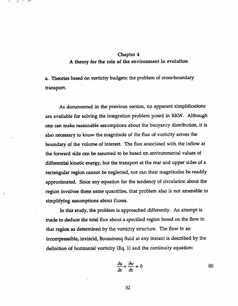
In this study, the problem is approached differently. An attempt is

made to deduce the total flux about a specified region based on the flow in

that region as determined by the vorticity structure. The flow in an

incompressible, inviscid, Boussinesq fluid at any instant is described by the

definition of horizontal vorticity (Eq. 1) and the continuity equation:

au aw -+-=0 ax (}z

32

(8)

Combining these expressions by differentiating Eq. 8 with respect to z and Eq.

1 with respect to x leads to the following Poisson equation describing w:

(9)

Once this equation is solved for w, u can be computed by integrating the

continuity equation from a lateral boundary upon which u is assumed to be

known. Thus, by assuming a vorticity structure, not only can the velocity

distribution be determined, but also the fluxes of vorticity across various

boundaries.

b. A simple three-region squall line

The observations discussed in Chapter 3 suggest that a squall line is

approximately described as a sloping zone of negative vorticity. This is

shown in Fig. 23 as the region labeled "i" (this name was chosen to since the

sloping region is generally near the interface between two distinct flow

branches). The slope of this vorticity zone is indicated by the angle a, as

shown in Fig. 23. As established in Chapter 3, evolution of a squall line is

characterized by the gradual tilting of this vorticity zone from an upright

orientation to a quasi-horizontal orientation.

The environmental wind profiles associated with the storms described

in Chapter 3, as well as with most squall lines examined in the literature

through observational, modelling, and theoretical studies, can be

approximated by a layer of about 3000 m depth with constant shear (from the

surface to height Zj), located below an upper layer with a different value of

constant shear. If shear "reverses" in the upper layer (Le. line-normal flow

becomes increasingly negative with height), the flow near Zj resembles a jet.

33

These ~FOftles will be discussed further in later sections. This , .:..

commonly observed two-layer structure to the environmental flow requires :,:!If-:.

that two'other regions of vorticity must be included on this simple model: a

lower environmental shear layer and an upper layer.

For this discussion, it will be assumed, based on observations, that the

vorticity in each ,region remains constant. In Fig. 24, the average vorticity in

the interior region of the six well-observed squall lines is depicted. The cases

are arranged, from a-f, in order of increasing rate of evolution. As described

in Chapter 3, it can be seen that vorticity becomes rapidly more negative

during the formative and intensifying stages, remains approximately constant

during the mature stage, and then increases gradually during the dissipating;:

stage. It is during the mature stage that a squall line tilts from its most erect .

orientation to quasi-horizontal, and it is this stage that is characterized by

relatively slow changes to the average vorticity.

In regions a and b, few observations are available to support the

assumption of constant vorticity. It is reasonable to expect that the forward

environment will be modified due to the presence of the squall line (e.g.,

Hoxit tt Ill., 1976, and LM). However, it will be assumed herein that the

environmental shear is steady. Thus, in this model, changes in circulation

are a~t1!d ~usively by changes in the areas of the regions, not by C'"'.,.. . . : ' ... ..:, .... ,~

~:i.~~~dty. This model is unquestionably highly simplified ... ~,,~' .' ,,,,;'" .;'

compal"!lf'l~l~ line and environmental flows, but it will allow for " " •.. "<1\ .• ," .:-\i-

some ~1lncIin8iittegarding the role of environmental shear. It does

include some of the typical squall line flow features, including a low-level

gust front, a sloping updraft, and a region of rear inflow (examples of the

Simplified flow are shown in the next section).

34

Circulation in this problem is defined as

C=J17' ndS s (10)

where 5 describes a vertically oriented surface orthogonal to the squall line

orientation, and n is the unit normal vector to the surface. Letting 11

represent the spatially averaged vorticity in each region,

(11)

is the circulation about the regions a, b, and i combined, where A represents

the area of the respective regions. Further, with vorticity constant, the

circulation tendency is simply

dC dAa dAb ~ -=-17 +-17b+-17" dt dt a dt dt'

(12)

It is assumed that the width of region i is fixed, so its area is constant

regardless of the slope. Thus any changes in circulation (as a result of

buoyancy effects, for example) about the combined region lead to changes in

the areas of regions a and b. In the atmosphere, the average vorticity in each

region could adjust to accommodate the circulation tendency, but in this

simple model it is required that the slope of the storm is the only feature that can

change. The impact and validity of these assumptions are addressed in later

sections.

In the three-region model described above, the area of region a is given

by

(13)

35

· .,.r-.•.... " '.~.:~.';t.:. ~;~

The area of region b is given by z~

A" =...:L . 2a

(14)

The area of region i remains fixed because it is assumed, that its width

remains approximately constant (based on observations of the storms

discussed in Chapter 3). Differentiating Eqs. 13 and 14 with respect to time,

with levels Zj and Zt fixed, and substituting in Eq. 12 yields an expression for

the tendency of circulation as a function of slope ex:

de 1 22 2da -=~[11 (Z'-Zt)-l1'~']- . m 2a· G J ~J m (15)

c. Determination of flow and vorticity fluxes

An alternative expression for the circulation tendency about a circuit

that is not a material curve,. where 1 is a unit vector along the curve and k is

the unit vector in the +z direction, can be expressed as

(16)

This equation shows that two processes can lead to changes in the circulation:

transport of vorticity across the boundaries and the generation of circulation ,,;-.;. '--4 .,.,.' ... ~ ,;~~ .: ... .: ••. :

owing 'to. buOyancy effects. The difficulties in evaluating the first term on the ...• ~~:~;.,....

right,tbeJilx' of vOJticity across the boundaries of a region, have already been ~ ~.~ ~ ~::;~.~~.~ t!t·J-" . '.~: > "'; • .'\~

documented: : . . .:,-

In this study, a new approach is used in an attempt to approximate

these terms. The Poisson equation for w (Eq. 9) is solved using a relaxation

technique. The vorticity distribution is as described in the discussion of the

three-region model shown in Fig. 23: constant vorticity with different values

36

in regions a and b, and negative vorticity in region i. The sloping vorticity

zone, region i, is assumed to have a linear increase in vorticity from a

specified minimum along the center line, hmin, to the surrounding ambient

value. The width of this zone is kept fixed at 10 km, a value very typical of

observed storms. Boundary values of w were specified to be zero at left and

right boundaries, well-removed from the sloping vorticity zone, and at z=O

and z=15 km. The vorticity flux term at the upper boundary is computed at

level Zt (6000 m) along the line from the rear of the sloping vorticity zone to

the right lateral boundary (upper bold line in Fig. 23). The vorticity flux was

also computed at the sloping rear boundary of the region i using the normal

velocity component. Vorticity flux at the surface is known to be zero since

w=O. In a series of experiments the slope a of region i, vorticity in region i,

and ambient upper and lower shear were varied over the entire range

observed in the cases described in Chapter 3, plus a large surrounding range of

values that encompass all squall line cases reported in the literature.

i) Flow as a function of inflow strength

The validity of the simple three region model is explored in this

section by examining the velocity distributions derived from its vorticity

structure. The vertical velocity distribution in this model is determined

entirely by the vorticity distribution. Thus changing the magnitude of the

horizontal flow at a boundary does not alter the distribution of w, but d~s

change the orientation of the streamlines.

Figure 25 illustrates this effect using a vorticity zone sloped at 45

degrees, shear of 4xl0-3s-1 (12 ms-1 over 3000 m depth) in the lower layer, and

37

no shear in the upper layer. In the case of strong inflow (18 ms-1 velocity at

the lowest level, shown in panel a), the updraft tilts rearward above a gust

front that has a surface location at x=37 kIn. With inflow of 12 ms-1, the

updraft issues vertically (as required in RKW), but is highly asymmetric.

With weaker inflow (6 ms-1 in panel c) the gust front is located near x=40 kIn,

slightly more forward than in the stronger inflow solutions, and the updraft

streamlines tilt forward with height.

The orientation of the updraft would seem to imply that there is a

minimum inflow strength required for rearward-sloping updraft trajectories,

prohibiting precipitation from falling into the inflow. However, this

sensitivity was not tested in this study. Since it is the actual trajectories of the

inflow rather than the streamlines that are important here, the propagation

speed would also playa role in determining whether or not precipitation is

deposited in the inflow.

Several important features of squall lines are shown in these solutions

based on the simple three-region model. A surface gust front is present at the

source region for the updraft. The updraft slopes rearward above the sloped

vorticity zone. Also, a rear inflow jet is present that descends toward the .

surface near the leading edge. The slope of the inflow jet may appear extreme

in these solutions, but the 45 degree slope of region i is quite large for a

mature squa11line as shown in Chapter 3. With more realistic slopes, the rear

inflow jet would descend more gradually.

38

ii) Flow as a function of vorticity zone strength

The effect of varying the minimum vorticity in the sloping region i is

illustrated in Fig. 26. The most obvious effect is the increase in the strength of

the perturbed flow with increasing magnitude of negative vorticity. In all

three solutions, the width of the sloping vorticity zone, inflow strength, and

ambient shears are the same. Interestingly, in panel c of Fig. 26, the ambient

vorticity below 3 km is equal to the minimum vorticity in the sloping zone.

Thus, this solution most nearly represents a "balance" between ambient and

storm-generated vorticity. However, this set of solutions shows that if an

"optimal" configuration is one with an intense updraft, it is preferable to

have much stronger storm generated vorticity than ambient shear, as in

panel a. On the other hand, if it is optimal to have a vertically issuing

updraft, another combination of shear and storm-generated vorticity is

desirable. The "balanced" solution leads to a rather weak, sloped updraft in

these particular combinations of parameters.

More subtle effects of varying the vorticity are also illustrated. The

flow at the lowest level has stagnation points ahead of and behind region i.

When storm-generated vorticity is small, as in panel c, the stagnation points

are closer to the centerline of region i. As storm-generated vorticity becomes

large, the stagnation points move away from the centerline.

39

iii) Flow as a function of slope

A major finding discussed previously is that the storm evolution is

described by the gradual tilting of the zone of negative vorticity, from erect to

quasi-horizontal. Fig. 27 shows the effect of tilting on the relaxation

solutions. The slope of region i in panel a is 1.0 (45 degrees inclined from

horizontal). Such a slope is quite extreme, and was usually only observed in

the formative and intensifying stages of the squall lines. At this slope, the

flow represents an updraft above a surface "windshift", with a trailing

downdraft and developing rear inflow.

In panel b, the slope is 0.5 (about 27 degrees). This also is a rather large

slope for the mature stage of a squall line, but was observed in at least one

case (26jan89s). At this slope, rear inflow has expanded and occupies a region

20-30 km in horizontal extent behind the leading edge. In panel c, the slope is

0.25 (about 14 degrees). This slope is quite typical of the mature stage of most

of the squall lines examined. At this slope, descending rear inflow in the

region below 6 kIn extends at least 60 km behind the leading edge. Thus, the

upscale growth of the squall line circulation can be approximated by the

tilting of the vorticity zone toward the horizontal.

These solutions are similar in many important respects to squall line

flows in the lowest 6 km. They all feature an updraft that begins near a

surface windshift region, and slopes upward and rearward. As the vorticity

zone (region i) tilts toward the horizontal, the updraft streamlines become

more horizontally inclined, and vertical velocities become weaker, in strong

agreement with the findings presented in Chapter 3. In addition, the

solutions show a downdraft region that, at large slopes, resembles convective

40

downdrafts, and as the system tilts toward the horizontal, resembles a

descending rear inflow jet. Again, these findings show striking similarity to

the gross features of structure and evolution described in previously. Panel c

of Fig. 27 also bears considerable resemblance to the conceptual model for a

"mature" squall line storm (Fig. 1).

One other, feature merits discussion. In this simple model, the strength

and orientation of the rear inflow jet is a function of the environmental flow

and the strength and orientation of the vorticity in region i. If the shear in

region b is strong enough to cause storm-relative RTF flow in the

environment, this flow penetrates to near region i. It remains "elevated"

when the region i vorticity is relatively weak, and it "plunges" when the

vorticity is relatively strong.

iv) Total flux determined from relaxation solutions

Several hundred solutions to Eq. 9 were assembled that span a large

range of lower and upper ambient shear, strength of the vorticity zone, slope, '

etc. The ranges of these variables that were used encompass all of the storms

observed in Chapter 3, and most (perhaps all) other published squall line

cases. This was done in order to find an expression for total flux as a function

of the other parameters.

Allowing only slope to vary, it is found that in all cases the total flux of

vorticity across the boundary shown with the heavy bold line in Fig. 23 is a

nearly linear function of slope up to about a=O.66 (approximately 38 degrees).

For more erect slopes, flux is approximately constant at the value

corresponding to a=O.66. This is illustrated in Fig. 28 for zero upper shear,

41

4xlO-3s-1 lower shear, and vorticity zone strength -lxl0-2s-1. This finding

greatly simplifies the process of determining an approximation for total flux

based on the other parameters. The dependence on a is linear, so it is only

necessary to approximate the total flux at (say) a=0.66.

Another major simplification results from the fact that total flux is not

a function of inflow strength. For given upper and lower shears, the wind

speed at any level (z=O, for example) determines the speed at all levels. In

this model, for a given vorticity distribution, w is determined. Thus the

transport through the upper part of the domain is a function of vorticity

distribution alone. Since w is fixed, increasing inflow at the right side of the

domain correspondingly increases rearward flow at the sloping rear surface

(mass is conserved in the domain). The vorticity distribution is the same at

both of these faces, so an increase in vorticity flux at one face causes an equal

and opposite transport at the other face.

With the simplifications just discussed, the process of determining

total vorticity flux (first term on RHS of Eq. 18) becomes one of fitting the flux

at a slope a=0.66 as a function of upper and lower shears and minimum

vorticity in region i. Several hundred relaxation solutions to total flux were

computed. The following expression describes the dependence of total flux

(Ft) on the other parameters:

Fr = -16.4 + 1. 78xl0317min + 1. 62x10617~

+1.12xl0717min17a - 9. 65x10317b - 1. 57x10717min17b

-1.13xl0717a17b + 1. 37xl0717~

(17)

Here, the subscript "min" represents the minimum value on the center line

of region i. Fig. 29 shows that this expression provides an excellent fit to the

total fluxes computed in the many relaxation solutions. It should be noted

that this expression is valid for the following ranges of parameters:

42

a ~ 0.66

-1. 5x10-2 < 11_ < 0

o < 11b < 1. 5xlO-2

-5xlO-3 < 11a < 5xlO-3

For slopes greater than a=0.66 (about 38 degrees), Ft can be approximated

using the value for a=0.66.

d. Slope, tilt, and the predictive equation for tilting

In this dissertation, the term slope (represented by angle a) is used to

represent the inclination from the horizontal of the sloping vorticity zone.

The term "tilt" is used as a verb to represent the change of slope, da/ dt. An

equation for da/ dt can be arrived at by combining Eq. 16 with Eq. 15 to yield

(18)

This expression is general, and not dependent on the relaxation solutions and

curve fitting described above. The technique described in the previous

section gives an expression for Ft which can be used to evaluate the effects of

environmental shear in the tilt of the sloping vorticity zone.

Eq. 18 indicates that one condition for steadiness (da/dt = 0) is for the

transport of vorticity out of the domain (Ft> to be exactly offset by the

generation due to buoyancy at the rear side of the domain. Another

implication of Eq. 18 is that as the slope approaches horizontal, the tilting

diminishes. And most important, the denominator can be of either sign

according to sign in the following inequality:

43

2 3: < T1a ZI T1a - T1b

(19)

The value of the denominator in Eq. 18 is shown in Fig. 30. It can be seen that

the denominator can take either sign over the range of shears observed in

squall line environments. In the region where the denominator is near zero,

Eq. 18 implies that tilting will be rapid, either forward or rearward depending

on the balance of integrated negative buoyancy and Ft. This region

corresponds to the physical situation of little net average vorticity in the

environment, so that very large changes of area are required to accommodate

any changes in circulation. Some implications of this are explored in later

sections.

e. A role of the environment in storm evolution

In this section, the role played by the environment in determining

tilting rate is explored. As an introduction, the nature of the solutions for a

given set of vorticity values in the three regions is shown graphically in Fig.

31. The nature of the curves can change dramatically as the shears are varied,

so this example should not be interpreted as illustrating the role of shear and

buoyancy across the parameter space. This particular set of curves is

presented to make one major point concerning the possibility of a steady

slope under the given conditions. The graph shows tilt versus slope for a set

of four combinations of shears and integrated negative vorticity, DCAPE

(Downdraft Convective Available Potential Energy). The term "DCAPE" is

used here because, as shown in Chapter 3, it seems that the region containing

the most negative buoyancy probably slopes up and rearward along the

underside of the ;;;loping vorticity zone, and is not confined to a surface-based

44

"cold pool." It should be noted that DCAPE is sensitive to the time of day,

since it involves the integrated difference between the environmental virtual

potential temperature ahead of the storm and the virtual potential

temperature of the negatively buoyant air in the storm. Thus, significantly

smaller DCAPE is to be expected with a nocturnal boundary layer compared to

a daytime bound,ary layer.

For certain values of DCAPE, one curve (open circles) shows that, for

any slope, the tendency is for the vorticity zone to continue to tilt rearward

(da/dt < 0). For other combinations (e.g. the curve with filled squares), erect

zones initially tilt rearward, but then slow and stop tilting as certain slopes are

reached. The observations presented previously indicate that in the

formative and intensifying stages, updrafts and negative vorticity zones are

erect. Thus this theory indicates that for certain combinations of shears,

storm-generated vorticity strength, and DCAPE, the storm will arrive at an

equilibrium slope and remain steady at that slope (presumably until

environmental shears or DCAPE changes). Additionally, it appears that if a

storm "finds itself' with slope shallower than the equilibrium slope, it will

become more upright until it reaches the equilibrium. In this section, the

general findings of this theory will be explored with regard to the possibility

of an equilibrium slope being reached. With yet other combinations, a

rearward-sloped storm will tend to become more erect (filled circles).

Figure 32 show the equilibrium slopes (defined as the slope above

which region i tilts rearward and below which region i tilts forward) as a

function of environmental upper and lower shear for three different values

of DCAPE. All of these graphs are for minimum region i vorticity of

-8xl0-3s-1, a typical value for the observed storms. Where the curves are

plotted, it can be said that a steady storm (da/ dt=O) is possible. More

45

specifically, it can be seen that as DCAPE increases (from panel a to c), larger

lower shears are required for steadiness. For the case of a DCAPE of

-1500 m2s-2, low-level shear must generally be larger than 1x10-2s-1 (30 ms-1

in 3 kIn) to "balance" the cold pool and lead to a steady system. Note that in

these results it is the magnitude of the low-level shear that is important, not

its transport (i.e., not differential kinetic energy). This is a consequence of the

fact that in this model, total flux of vorticity (Ft) does not vary with

environmental flow strength, but only with vorticity.

It can also be seen in Fig. 32 that as upper shear goes from negative to

positive, the possibility of a steady, rearward-sloping, quasi-2D squall line

becomes more remote. Finally, as low-level shear increases for a given upper

shear and DCAPE, the equilibrium slope becomes shallower. In light of

RKW, this seems counterintuitive. However, the explanation is

straightforward: as low-level shear increases, the total flux (Ft) increases. For

a given large slope (a), the flux is more than sufficient to balance the cold

pool, leading to a numerator in Eq. 18 that is positive. All of these curves fall

in the region of Fig. 30 in which the denominator of Eq. 18 is less than zero, so

rearward tilting is expected for the assumed large slope. Thus as low level·

shear increases, the tilting tendency is increasingly negative at large slopes.

Therefore tilting tendency does not go to zero until shallower slopes are

reached.

If this theory is correct, it appears that the intuitive concepts proposed

by RKW must be reconsidered. Storm structure and evolution is a function

of the degree of balance between DCAPE and total flux. However, total flux is

a function of the slope of the storm and the shear in both the lower and upper

levels. The implications of Eq. 18 will be further illustrated in later sections

where observations and previous modelling results are considered.

46

The data presented in Fig. 32 pose a forecast dilemma: as low-level

shear increases, a sudden transition is made from conditions in which no

steady rearward-sloped storm is possible, to those supporting an erect, steady

storm. Presumably the erect configuration would also imply a relatively

more intense storm, since updraft magnitudes would be larger and confined

to a narrower b~d.

As a final illustration of the predictions of this theory, the average

DCAPE that can lead to a steady storm (da/ dt=O) is shown in Fig. 33a for a

variety of shears. The minimum vorticity in region i is again assumed to be

-8xlO-3s-1. Where curves are not plotted, a steady rearward-sloping squall

line is not possible. One general finding is that larger DCAPE can be balanced

by increasing low-level shear, as argued in RKW. Another finding is that

upper-level shears less than zero (reverse shear) supports allows stronger cold

pools to be associated with steady storms. In Fig. 33b, the full width of the

range of cold pools associated with steady storms is shown. The clear

interpretation is that a very wide range of DCAPE can lead to steady storms if

the low-level shear is large (these steady storms will have a variety of

equilibrium slopes). On the other hand, as upper shear increases and/or low-"

level shear becomes smaller, the storms require a more exact DCAPE for

steadiness.

f. Comparison to observed cases

In this section, the predictions of the theory are compared to the seven

cases from Chapter 3, in which the mature stage and tilting rate were well

documented. In order to evaluate the theory, soundings were used that were

nearest in time and space to the leading edges, yet appeared to be unaffected by

47

the squall lines. The shears below and above 3 km were estimated by

approximating the line-normal velocity profile with straight lines in those

layers. A good technique for estimating integrated negative buoyancy has not

yet been developed. For these tests, DCAPE was evaluated as the integral of

the difference between the sounding wet bulb temperature profile and the

environmental t~mperature below 6 km. The tilting rate equation was

evaluated for this particular value of DCAPE + / - 30%. This range should

allow the effects of condensate loading, vertical redistribution of cooled air,

and other effects to be represented. Since soundings were not generally

available to the immediate rear of the leading edge of these systems, any

refinement to the estimated DCAPE would be highly speculative.

Earlier in Fig. 24, the slope a of the six well-observed squall lines was

depicted as a function of time (solid curves). The cases are arranged from a-f

according to a crude estimate of rate of tilti:ng during the mature stages. These

cases are examined in that order: slowest-evolving to most-quickly evolving.

The environment of the storm denoted 26jan89s (the slowly evolving

system on 26 January 1989 from DUNDEE) is examined in Fig. 34. As shown

earlier in Fig. 24a, the vorticity zone in this storm essentially oscillated about

a very large slope; hence it was quasi-steady. The estimated DCAPE of this

storm was in the range -569 to -1057 m2s-2. The storm-relative line-normal

wind component had large shear below the jet (4x10-3s-1), and relatively large

"reverse" shear above the jet (-1.2xlO-3s-1). It can be seen that the

environmental flow is front-to-rear at all levels. Although rear-to-front

relative environmental flow occasionally was observed in DUNDEE, in

general the flow was front to rear in substantial agreement with the

observation of Zipser (1977) of tropical squall lines having relative inflow

(front-to-rear) at all levels. The solutions for the tilting in this environment

48

are also shown in Fig. 34c, using an assumed minimum vorticity in the

sloping zone of -8x1o-3s-1. This value is fairly typical of the systems analyzed;

the observed range was approximately -6x10-3s-1 to -10x10-3s-1. The curves

are not especially sensitive to this parameter in most cases. The graph has a

simple and clear interpretation: an initially erect storm will tilt fairly rapidly

rearward. As it does, the rate of tilting rapidly goes to zero, so that the storm

will eventually stop tilting and reach a steady configuration. For the

sounding-derived DCAPE, equilibrium occurs at slopes greater than 30

degrees, in strong agreement with the observed equilibrium slope (Fig. 24).

Two other curves are shown for smaller DCAPE, showing that as DCAPE is

reduced, equilibrium occurs at shallower slopes.

Another rather slowly-evolving storm occurred during DUNDEE on 26

November, 1988 (26nov88s). Fig. 35 depicts the environmental conditions, as

well as the solutions for rate of tilting for this storm. DCAPE is estimated to

have been between -670 and -1244 m2s-2, with an upper shear of about

-1.8xlO-3s-1 and a lower shear of about 3.9x10-3s-1. The solutions for this case

are unique among the six cases in that it appears that a storm with DCAPE

near or less than -670 m2s-2 and a slope of more than about 25 degrees will

become more erect with time. The early history of this squall line is not

known, since it formed beyond the range of the radar coverage. However, in

Fig. 24 it can be seen that the storm generally had a slope less than 25 degrees,

and in fact tilted only very slowly rearward with time. This seems to be in

substantial agreement with th~ prediction of the theory for the observed

slopes.

Another relatively slowly evolving storm occurred during the PRE­

STORM on 10-11 June, 1985 (10jun85m). Fig. 24 shows that this storm tilted

rather slowly rearward until it reached a slope of around 10 degrees, at which

49

time it appeared to be steady. This is a remarkably shallow slope for the

vorticity zone; the storm's apparent vigor even at these shallow slopes can be

attributed to the unusually strong storm-relative inflow, a condition which

implies stronger-than-usual ascent for a given slope. The environmental

conditions and solution for tilting are shown in Fig. 35. The curves are

similar to those for 26jan89, in that they show a comparatively slow tilting

rate, and the likelihood of steadiness. In contrast to 26jan89s, it appears that

this storm should become steady at a much shallower slope (12-21 degrees),

which is well supported by the observations (i.e. this storm became steady at a

much shallower slope than 26jan89s).

A more quickly evolving storm occurred in DUNDEE on 7 February,

1990 (7feb90m). The environment (Fig. 37) contained weaker average shear in

the low levels (about 5x10-3s-1) than the three previous cases, as well as

weaker reverse shear above the jet (about -lxl0-3s-1). DCAPE was estimated

to have the second-largest magnitude of the six cases (-889 to -1651 m2s-2).

The solution for tilting for this case disagrees with the observations (Fig. 24).

However, note from Fig. 30 that the denominator in Eq. 18 for this case is very

close to zero. This implies fairly rapid evolution (unless the flux and DCAPE

are very nearly balanced) but the sign of tilting is somewhat uncertain. This

is an interesting part of the parameter space. The physical implication based

on this theory is that evolution is rather unpredictable in this vicinity.

The last two storms illustrated in Fig. 24 evolved very quickly (other

storms were observed which e:volved so quickly that the mature stage was too

short for estimates of tilting rates to be obtained). The environmental

conditions for the DUNDEE storms on 5 December 1989 (5dec89f) and 18

November 1989 (18nov89f) are shown in Figures 38 and 39 respectively. It can

be seen that both cases had relatively weak shear in the lower levels

50

(2.4x1o-3 5-1 and Sx10-3 5-1 respectively) and moderate reverse shear above

(about -2xlo-3 5-1). DCAPE in the case 5dec89f was estimated as -547 to -1012

m2s-2, the weakest of the six cases, whereas in 18nov89f it was -982 to -1824

m2s-2, the largest of the six. The solution curves for both cases correctly show

that a steady storm is not possible. Rather, in both cases storms at any slope have

the tendency to tilt further rearward.

In summation, the theory expressed by Eq. 18 correctly predicts the

possibility of steadiness, the approximate slope at which steadiness occurs,

and the correct sense of the rate of tilt (except for 7feb90m). It should be

pointed out that, despite these strengths, the theory predicts tilting rates that

are too large by an order of magnitude or more (-0.1 deg s-1 vs. the observed

rates of -O.Olrleg s-I). Possible reasons for this overprediction are discussed in

later sections.

g. Comparison to other observations

Herein predictions of Eq. 18 are compared to observations based on

other published studies. Bluestein and Jain (1985) described an echo category

they termed ''broken line" which most nearly resembles the typical echo

patterns of quasi-two-dimensional squall lines described herein. Using their

published average line-normal wind components and standard deviations,

the average low-level shear for their "broken line" classification is

approximately between 0.7xl0-3 s-l and 4xl0-3 s-l. The average shear from 3

to 6 km is approximately between -0.7xl0-3 s-l and 2.7xl0-3 s-l. The 26 May

1976 squall line in Oklahoma (Ogura and Liou, 1980; Smull and Houze, 1985;

1987) is one example of a storm that occurred within this range of shears.

Referring to Fig. 33 it can be seen that these shears should be associated with

51

I

stonns falling well outside the ranges associated with steady systems except

perhaps those with unusually small DCAPE. Another classification that

seems to encompass the quasi-two-dimensional squalilines discussed herein

is the "strongly classifiable symmetric" class of Houze et al. (1990), identified

from climatological studies of Oklahoma squall lines. Their values of lower

shear (1.2xlo-3s-1) and upper shear (1.8xl0-3s-1) fall into the same parameter

space as those given by Bluestein and Jain for squall lines in the same region.

Solutions to Eq. 18 spanning the likely range of cold pools strengths are

shown in Fig. 40. It can be seen that for all values of OCAPE with these two

given shears, the vorticity zones tilt forward regardless of the slope.

For all of the available mid-latitude data discussed above (except for the

10-11 June 1985 PRE-STORM case described above), it appears that the low­

level shear is too weak to allow for steady, rearward-sloped storms. The

possible exception to this finding is for mid-latitude cases occurring at night

when DCAPE is much smaller due to the relative coolness of the nocturnal

boundary layer. Under the "typical" middle latitude environmental

conditions, it appears that steady, rearward-sloped systems are quite possible

at night, but highly unlikely during the daytime, due to the expected changes

in OCAPE.

It is likely that many of the daytime middle latitude systems examined

as individual cases or part of climatological studies, are not quasi-2D,

rearward-sloped steady systems. It is interesting that in examining the slab.

averages of reflectivity for the tropical systems, even at 10 minute temporal

resolution, individual cells were not seen propagating rearward from the

leading edge, and horizontal depictions of reflectivity showed very uniform

structure to the leading edge compared to published middle latitude cases.

The conceptual model based on middle latitude systems features rearward-

52

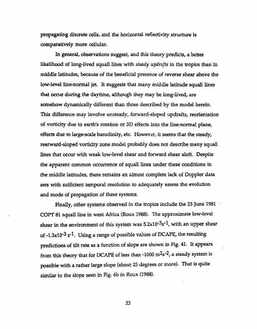
propagating discrete cells, and the horizontal reflectivity structure is

comparatively more cellular.

In general, observations suggest, and this theory predicts, a better

likelihood of long-lived squall lines with steady updrafts in the tropics than in

middle latitudes, because of the beneficial presence of reverse shear above the

low-level line-normal jet. It suggests that many middle latitude squall lines

that occur during the daytime, although they may be long-lived, are

somehow dynamically different than those described by the model herein.

This difference may involve unsteady, forward-sloped updrafts, reorientation

of vorticity due to earth's rotation or 3D effects into the line-normal plane,

effects due to large-scale baroclinity, etc. However, it seems that the steady,

rearward-sloped vorticity zone model probably does not describe many squall

lines that occur With weak low-level shear and forward shear aloft. Despite

the apparent common occurrence of squall1ines under these conditions in

the middle latitudes, there remains an almost complete lack of Doppler data

sets with sufficient temporal resolution to adequately assess the evolution

and mode of propagation of these systems.

Finally, other systems observed in the tropics include the 23 June 1981

COPT 81 squall line in west Africa (Roux 1988). The approximate low-level

shear in the environment of this system was 5.2xl0-3s-1, with an upper shear

of -1.3x1o-3 s-1. Using a range of possible values of DCAPE, the resulting

predictions of tilt rate as a function of slope are shown in Fig. 41. It appears

from this theory that for DCAPE of less than -1000 m2s-2, a steady system is

possible with a rather large slope (about 25 degrees or more). That is quite

similar to the slope seen in Fig. 6b in Roux (1988).

53

h. The findings of RKW and LM interpreted through this theory

This theory embodies, albeit crudely, some the system-scale effects

described by LM as being important to squall line longevity. To the extent

that quasi-2D squall lines are represented by sloping vorticity zones embedded

in a two-layer environment, these features are included. As described

previously, these include a rearward-sloping updraft, a possible overturning

updraft branch, and descending rear inflow branches of various strengths and

configurations. Clearly, this is a highly simplified model, but it implicitly

represents a much broader scale of influences than a simple cold pool/low­

level shear balance.

Based on numerical modelling studies, Thorpe et al. (1982, hereafter

referred to as TMM), demonstrated that even with low-level shear held

constant, the shear above had profound influences on the resulting storm

structure and evolution. Using their shears, and a DCAPE of -800 m2s-2, the

theory herein predicts results (Fig. 42) similar to those reported by TMM. For

instance, it appears that for strong forward shear, denoted "P( + 10)" in TMM~ a

forward-tilting vorticity zone is likely. Presumably, in a 2-D simulation, this

system would deposit precipitation into its inflow, thereby reducing potential

buoyancy and storm longevity. TMM report that the P(+10) storm consisted

of essentially one pulse of convection followed immediately by decay. The

P( +5) simulation produced a "vigorous second cell" which also decayed

rapidly. This is an interesting finding in light of the discussion above

concerning the middle latitude squall line cases, and lends credence to the

speculation that, where the present theory p~edicts slow forward tilting, squall

54

lines are possible but their leading edge convection will exhibit pulsing

behavior, or the commonly reported "succession of cells" in the 2-D structure.

The remaining curves suggest steady, rearward-sloped storms. The

smallest predicted equilibrium slope is associated with "reverse" shear of 10

ms-1 aloft, while the most erect is associated with no shear aloft. These

correspond to the "P(-lO)" and "P(O)" storms in TMM. Their results indicate

that the longest-lived storm occurred with no shear aloft, and the theory

herein predicts that this storm should indeed be steady. With the shallower

equilibrium slope, the theory implies that the "P(-lO)" storm should deposit

precipitation over the largest rearward-extending region, which it did in the

simulations of TMM. Computations for other values of DCAPE indicate that,

for this particular set of shears, the tilting rates and equilibrium slopes are

highly sensitive to DCAPE. Despite this fact, it is clear that a variety of

possibilities for steadiness and equilibrium slopes are possible when only

upper shear is varied, in complete agreement with the findings of TMM.

RI<W did not consider the role of upper shear. In their study, upper

shear was held constant at zero, while lower shear was varied in a search for

an optimal value. Using a velocity profile containing no shear in the upper

levels, Eq. 18 predicts that the optimal lower shear is approximately where

RKW predicted it to be. Although DCAPE in the RKW simulations is not

known, for a strength of -600 m2s-2 the most erect, steady storm should occur

with a lower shear of about 7xl0-3s-1, exactly as found by RKW (see Fig. 43).

With a OCAPE of -1200 m2s-2, this "optimal" shear value increases to around

9xl0-3s-1. Other "optimal" values of DCAPE for wind profiles with no upper

shear can be found in Fig. 33 along the line where ambient upper shear equals

zero.

55

The RKW theory involved only cold pool strength and vorticity

transport from the environment in the lower levels in an attempt to explain

strong, long-lived squall lines. The RKW approach, and the need to verify

their conclusions from an observational perspective, motivated this study. In

light of the agreement between observations, modelling work, and

observations shown in the present paper, it does appear that lower shear and

OCAPE need to be considered together with upper shear and system slope

when drawing conclusions about intensity and longevity.

56

Chapter 5

Discussion

Examination of the various cases documented observationally in this

study reveals common features in the reflectivity and kinematic structure of

these squall lines which can be associated with the stages of evolution. Of

primary importance is the observation that although the storms undergo

common patterns of evolution, the time scale over which the evolution

occurs varies greatly among systems. Combined durations of the formative,

intensifying, and mature stages of the stonns varied from about an hour

(18nov89F, 5dec89F), to over four hours (26jan89S). Measurements of the

rate of change of slope of the vorticity zone in the jump updraft region shows

that these systems may span an order of magnitude in evolution rates.

Another observation of major importance is that the structure of this type of

squall line is characterized by a sloping zone of horizontal vorticity, with

streamlines approximately parallel to the vorticity zone. The evolution is

characterized by the gradual tilting of this vorticity zone toward the

horizontal. During the intensifying stage the sloping zone of negative

horizontal vorticity develops, strengthens, and reaches its most upright

orientation. During the mature stage, its strength remains about constant

while it tilts toward the horizontal. During the dissipating stage, its

orientation remains quasi-horizontal, and the vorticity weakens. These

57

generalizations seem to apply across a fairly large range of storm intensities

and relative flow strengths.

Observations of features that can be used to classify storm stage are

summarized in Table 2 and in 'Fig. 45. Because the structure of the flow and

reflectivity change so much from one stage to another, the "snapshot"

structure of a squall line depends strongly on the stage of evolution. For this

reason, the

Table 2: Characteristics of sQuall line evolutionmy staus.

STAGE

Cbaracteristic Founative Intensifyin~ Mature Dissipatin~

Horizontal Scattered or Soild line of Solid line of Cellular leading reflectivity broken cells in a cells. Trailing cells. Large becoming structure line region fonns trailing region. patchy.

Transition zone Stratiform weakens

Vertical Deepening Reaches Gradually Shallow, reflectivity deepest, most becomes relatively weak structure intense, and shallower, cells or

most upright weaker, and stratiform ascent more tilted

Vertical Increasing Increases more Gradually Small velocity in quickly to decreases leading edge maximum

values

Motion Generally less Continued Suddenly faster; Varies than the mean relatively slow resembles cold flow pool

propagation speed

Slope Varies Most upright Gradually more Quasi-horizontal horizontal mesoscale flow

branches

58

features depicted in conceptual models of squall line structure (e.g. Fig. 1)

should be interpreted with caution as such a model may be a synthesis of

features that occur at different times during the life cycle instead of typifying

any certain stage. The rate at which evolution occurs in the squall lines

described here makes any assumptions about steadiness of questionable

value. Before a system is assumed steady from a dynamical viewpoint, a

careful analysis of the relative magnitudes of terms in predictive equations

should be made. In general, a priori assumptions of steadiness may not be

justified when describing squaUline dynamics.

The squall line examples presented herein, as well as the additional

cases analyzed, but not discussed in detail, make it clear that the generation of

vorticity is a system-scale phenomenon, as proposed by Lafore and Moncrieff

(1989). This can be seen by examining the slab-averaged horizontal vorticity

for the cases presented. Negative horizontal vorticity develops across the

system shortly after the leading edge first becomes solid. The appearance of

negative vorticity aloft to the rear of the leading edge seems to occur much

too quickly to be attributed to advection rearward from some leading edge

generation region alone. It appears that there is not a distinct separation

between the negative horizontal vorticity in the low-level cold pool near the

leading edge, and the vorticity that appears at higher elevations rearward of

the leading edge (except perhaps during the dissipating stage). Instead, a

nearly continuous zone of negative vorticity strengthens fairly uniformly

across the system with time. 1?is implies that important buoyancy gradients

occur across the entire squall line and through most of its depth, not just near

the leading edge of the low-level cold pool.

It is apparent from the data presented, that once a squall line becomes

more-or-Iess solid at its leading edge, the buoyancy distribution leads to the

59

generation of negative vorticity to the rear of the leading edge. The flow

structure associated with this vorticity is such that ice particles are carried

rearward, relative to the leading edge, in the upper portion of the trailing

region. Sublimation, melting, and evapontion below and to the rear of this

expanding cloud, as well as condensate loading near the leading edge, should

lead to a negative buoyancy anomaly along the sloping lower boundary of the

trailing stratiform cloud. Heating due to condensation and freezing should

maintain a positive buoyancy anomaly in the cloudy region as long as ascent

persists. These anomalies produce a horizontal buoyancy gradient across the

system, aiding in vorticity generation in the interior. One consequence of the

generation of negative vorticity in the storm interior, under certain

environmental conditions is that the strongest drafts gradually tilt from

nearly vertical during the formative stage, to nearly horizontal in the

dissipating stage, and the scale grows from that of convection to mesoscale.

The demise of the squall line is apparently caused by the tilting process as it

reorients the major drafts to quaSi-horizontal slopes.

With respect to the role of upper level jets and ambient baroclinity in

causing the development of a rear inflow jet, almost all of the cases studied

developed significant rear inflows of 5-10 ms-1. In some cases, rear inflow

magnitudes of 10 to 20 ms-1 relative to the motion of the leading edge were

present. The development of rear inflow did not depend on the presence of

an upper jet impinging on the storm from the rear, which is the causative

factor cited by Zhang and Gao (1989) in their modelling study of the 10-11 June

PRE-STORM case. In several cases with significant rear inflow, there was no

environmental RTF flow relative to the motion of the surface position of the

leading edge. From the vorticity viewpoint, rear inflow should be expected to

result from the storm-generated buoyancy gradients (as shown by Fovell and

60

Ogura, 1988) which lead to the generation of horizontal vorticity across the

storm. While the "blocking" of middle- and upper-level momentum may

indeed playa role in the rear inflow dynamics, it is not a sole causative role.

The observations indicate a strong connection between the occurrence

of horizontal convergence and negative vorticity. It can be shown that such a

correspondence is to be expected when the vorticity is due to shear alone

between uniformly tilted streamlines. Thus the mesoscale ascent often

observed in the upper part of the interior region, and mesoscale descent

below, are a function of the magnitude of negative horizontal vorticity as

well as the slope of the vorticity distribution. As tilting proceeds, the

mesoscale ascent weakens until the streamlines in the interior region become

horizontal. However, the velocity data suggest that there are pockets of

vertical motion occurring in the upper portion of the interior region on a

scale much more like that of the leading edge convection.

In one respect, the large magnitudes of negative vorticity generated in

the storm interior tend to lead to additional generation of vorticity. This is

because the shearing flow associated with the vorticity brings potentially

cooler air beneath the saturated, precipitating anvil cloud, or in another

frame of reference, draws the anvil cloud rearward over the potentially cooler

air. In this way, the negative buoyancy anomaly at the rear of the system,

beneath the anvil cloud, can be reinforced through diabatic processes. This in

turn maintains the horizontal buoyancy gradients that cause additional

vorticity generation.

It has been shown that the simplifying assumptions made by RI<W do

not seem to apply generally when the observations are examined. It is also

clear from observations, as well as the work of TMM, that squall line

61

structure and evolution seem to be sensitively influenced by upper shear, not

just by a balance between low-level vorticity transport and DCAPE.

Motivated by these observations, a new theory has been developed and

tested which considers the roles of both lower and upper shear, as well as

OCAPE, the strength of storm-generated vorticity, and storm slope as

measured by the. slope of the negative vorticity zone. There is much evidence

that this theory offers improved predictions of storm evolution and the

possibility of steadiness. The theory also makes it clear that storm slope and

upper shear play roles as important as DCAPE and low-level shear in

determining squal1line behavior.

There are numerous potential problems with this theory that must be

reiterated. Some of these potential problems are inherent to the dynamical

approximations made (e.g. two-dimensionality, inviscid fluid, Boussinesq

approximation applied over a deep layer, etc.). A major issue that has not

been addressed in this theory is the role of updraft available potential energy

(CAPE), which is often significant below 6 km. In the context of the three­

region model, the only role of CAPE that has been neglected would be to give

a positive vorticity tendency in the upper region (region a) ahead of the

storm. This would clearly have an effect on the circulation tendency and

tilting rate, since it was assumed that vorticity is constant in each of the three

regions. Another potentially important physical process that has been

neglected is mixing. Mixing could transport the negative vorticity from

region i into regions a and b ahead of the storm, thereby giving a non-zero

tendency to the average vorticity in these regions. It is felt that mixing does

playa large role in this regard, and that if mixing were somehow included in

this model, the predicted tilting rates might be much closer to those observed.

On the other hand, in a system with a very shallow slope, mixing between the

62

cold pool and inflow over the long inflow trajectories could mean that the

system would no longer survive.

Also, it seems likely that storms do modify their environments and

this also would lead to non-zero vorticity tendencies in the environment. In

fact, from the standpoint of this theory, the only way a steady storm could

eventually begin, tilting again and dissipate is for changes to occur in the

environment, either through storm modifications or larger scale or diurnal

processes. From a prediction point of view, it is hoped that despite the

changes that occur in the environment, the storm probably stays in one

general part of the parameter space, and hence the general characteristics of

structure and evolution remain predictable. Finally, no attempt has been

made to understand how the strength of the vorticity in the sloping region i

relate to environmental characteristics. The observations suggest that this

parameter is generally between 6xlO-3s-1 and lxlO-2s-1, and the solutions to

the tilting equation do not seem especially sensitive to this parameter over a

large range of ambient shears and DCAPE. Despite the shortcomings, it seems

that for observed cases and other modelling results in which enough

information is available to document structure as well as evolution, this

simple theory produces meaningful results.

In general, this theory indicates that, as low-level shear increases, larger

DCAPE is associated with steady rearward-sloped storms, and that steady

storms can occur over a larger range of DCAPE. It also shows that steady

storms are more likely with reverse shear aloft (Le. with a low-level line­

normal jet profile) than with forward shear aloft. Thirdly, if the reverse shear

is too strong and/or lower shear too weak, no steady system is possible

(storms continue tilting rearward until they collapse).

63

Fig. 44 presents one more look at the question of the structure and

evolution of mid-latitude versus tropical squall lines. This figure is a

duplicate of Fig. 33 with certain ranges of shears for various storms

superimposed. The box in the middle left portion of the picture is an

approximation of the range of shears, using mean line-normal wind profiles

+/- one standard deviation, derived from Bluestein and Jain (1985) and

associated with the broken line form of severe squall lines in Oklahoma. The

Houze et. a1 mean condition for strongly classifiable symmetric systems in

Oklahoma falls within this same box, as well as the 26 May 1976 Oklahoma

squall line investigated by several different authors. The range of shears for

the tropical squall lines, including those from DUNDEE, the 23 June 1981

COPT 81 squall line (Roux, 1988, marked "Roux"t and the 22 June 1981 COPT

81 squall line (Chong et al., 1987, marked "Chong") is denoted by the second

box in the lower center, with individual data points marked. Finally, the lO­

II June 1985 PRE-STORM squall line is marked "10jun", and is found quite

removed from the other middle latitude storms.

It is likely that DCAPE in middle latitudes is similar in magnitude to

that in the tropics: although water loading contributions are smaller, the

contribution due to evaporation is likely larger. If the present theory is

correct, it suggests that many middle latitude storms occurring during the

daytime do not feature draft structures described by steady, rearward-sloping

vorticity zones. However, steady rearward-sloping storms become more

likely during the night when DCAPE is reduced due to cooling in the

boundary layer. Perhaps the three-region model does not even apply to the

daytime storms in the part of the parameter space determined from the

Bluestein and Jain (1985) data. Or perhaps these systems have forward-tilting

draft structures that are continuously regenerated through discrete

64

development at the gust front or gravity-wave induced propagation. Also

possible is that the role of earth's rotation, perhaps in terms of inertial

stability, or the role of the often-observed vortex features in the stratiform

region, must be considered. All of these issues will remain unresolved until

the evolution of a number of middle latitude squall lines can be documented

with adequate temporal resolution.

65

Chapter 6

Conclusions and suggestions for additional research

The scope of this study is limited to a description of the evolution of

quasi-two-dimensional squall lines that feature a continuous, rearward­

sloping vorticity zone, and a possible mechanism for environmental control

of this evolution. It does not address the conditions necessary for the

initiation of a squall line. Also, storms with a system-scale three­

dimensionality, and those consisting of well-separated thunderstorms in a

line, have not been examined. The main emphasis herein has been on a

description of events and processes that occur during one cycle of

intensification and decay. Many of the squall lines analyzed exhibited very

prolonged dissipating stages, and it appears that squall lines can progress from

a deep convective mode, to one of much shallower, less-organized, but

persistent leading edge convection. Also, in several of the systems, deep

leading-edge convection recurred after a prolonged period of the dissipating

stage. It is plausible that such regeneration is due to changes in the

environment, or to weakening or slowing in the propagation of the cold pool

after it surges ahead of the dissipating leading edge. These issues merit

further research.

A simple vorticity budget approach to understanding squall line

dynamics is employed in this study. Approaches of this type require many

simplifying assumptions in order to obtain meaningful solutions. Based on

the predictions of the theory presented herein, it seems that this approach is

66

an improvement over that used by RKW, primarily because the effects of

upper shear are accounted for, and the allowable storm morphologies much

more closely correspond to ob~ervations. However, it seems that the limit to

this type of approach has probably been reached, and further advances must

come through numerical modelling.

H the findings of this study are correct, future numerical simulations

should systematically explore the parameter space described by low-level

shear, upper shear, and DCAPE. It appears that for this class of storm, two­

dimensional simulations may be adequate. However, in light of the

fundamental role of DCAPE (also see Emanuel, 1989), it will be vitally

important to correctly model the buoyancy distribution in the part of the

storm featuring negative buoyancy.

Some fundamental aspects of squall line dynamics remain to be

explored observationally. The evolution of middle latitude squall lines has

not been adequately documented. The present theory suggests that middle

latitude squall lines with large DCAPE are dynamically different from

"typical" tropical squall lines; it appears that a quasi-two-dimensional system

with a continuous vorticity zone should not occur in weakly sheared

environments with large OCAPE. Rather, it is suspected that in these

environments squall lines consist of much more cellular, unsteady leading

edges, and that organized rear inflow probably does not penetrate across the

entire storm to the leading edge. Though fundamentally unsteady at the

convective scale, it should still be possible to have a long-lived system that

appears quasi-steady at larger scales. And from a climatological perspective, it

seems that at night, since DCAPE decreases with boundary layer cooling, the

possibility of steady systems like those described in this dissertation becomes

much greater.

67

This study, because of its focus on two-dimensional dynamics, has

emphasized events that occur relatively early in the life cycle of a mesoscale

convective system (Maddox, 1980). A squall line that tilts rearward and

dissipates is not likely to grow upscale into a longer-lived mesoscale

convective system (except perhaps if convection repeatedly regenerates at the

gust front). However, for those environments capable of supporting a steady

system, growth will occur upscale through the mechanisms described in this

dissertation, and the possibilities that the system will evolve toward inertial

stability and geostrophic balance [a definition of an MCC proposed by Cotton

and Anthes (1989), p. 673] are much enhanced. For this reason, among others,

further research into the dynamics of squall lines is definitely needed,

especially in the middle latitudes. Future observational programs must

obtain Doppler radar data at intervals of about ten minutes or less over the

longest possible periods in order to be useful. Observational data sets that

provide infrequent snapshots of storm structure are of comparatively little

use. Reliable methods to assess the in-storm buoyancy structure also are

needed, as well as realistic techniques to estimate DC APE from pre-storm

soundings.

Finally, this work provides a basis for a re-examination of the derecho

phenomenon (Johns and Rirt, 1983). A cursory examination of the data

published thus far indicates that derechos may occur in environments

supporting steady, rearward-tilted systems. If derechos are in this class, it will

be interesting to find out what makes them an especially intense variation on

this basic storm type.

68

A

::::> Storm motIon

Gu.t fron' ".Iur. c.1I ~ ..

hIIIwr-ect • ...... B

Figure 1. Conceptual model of the line-normal s~cture of a squall line (adapted from Houze et aI., 1989).

69

14.0 r"'I""T""I"''T'''"r~~'T"T"T'''T''''T'''''~'''''''"T'''T"''1'''''I~T'"''T"T'''T-r-r-r-T'T"T'''T-r-I'''T"T"T'"T'''T~'''''''''''''''''''I'''''T''''''''''''''

50. 60. 70. 80. 90

Figure 2. A single cross-section of line-normal horizontal velocity from the 2-3 August 1981 CCOPE squall line (from Schmidt and Cotton, 1989). Stippled regions represent flow left-to-right. Velocity values are storm­relative.

23 JUNE: 1981 2322 YO-20km ~~-------------------------Z~--------------~~--------~

o

---.~"',/ *,-' .--., .. --.,.,--"~ .. , ... , ... " .. ,!,., ..... ·,,··1 ,., - - - - • • • , , - - , I , . ,

..... ·---·-·~'··'I'·' e . . • • .. - - - , , , . , , , . ,

..J: ••• ··._-",."1.'

.... ~ a:

o 10 20 X(kml

.,,--

UI'.;..~ .... ___ ~--~ ... -- -

30 40

Figure 3. Storm relative velocity vectors for the 23 June 1981 COPT-81 storm (from Roux, 1988). Solid contours are radar reflectivity values in dBZ.

70

..

-..J C)

« E

..lIC -

-70 -60 -50 -40 -30 -20 0 10 EAST - WEST DISTANCE (km)

Figure 4. Average line-normal velodty in the 22 May 1976 Oklahoma squall line (from Smull and Houze, 1987b). Negative values indicate flow from right-to-left.

lOO~----~~----~-----T~----~rT----~--------~--------~----~ u

200~ ___

300

_ 400 ~ e -

-180 -135 -90

,.--....... .... "" ----5-- __ -..... -I ..... -----'"

) ,_--- 10 ___ ' /

..... -- " ---- -5 __ /

0----===

--- -15 -_-.I -45 0 45 90 180

x (km)

Figure 5. As in Figure 4, but based on rawinsonde analysis (from Ogura and Uou, 1980).

71

&

(0) (b)

120

~ 120

I ~

a 20 l5 II) 80

a 20 .!I 60

40 40

]' 0 + 0 -...;

>-! lit"

-4Q 1" ..... -40

. ~. ...... . .....

-8) -8)

• -120 -120 I

-~2O -00 -40 0 40 eo 120 -120 -aJ -40 0 40 !rl ~2G

x (Icm) x (In'!)

Figure 6. Horizontal reflectivity maps for the formative stage. The radar is at the" +" symbol, with the parallel lines denoting the region for vertical cross-section slab averages used in later figures. Horizontal axes labeled in km from radar. a) 5 December 1989 tropical case, 0710 UTe. b) 10 June 1985 middle latitude case, 2319 UTe.

-7 1-

""","," (0)

20

16 , ~ 5decB9F' -071MC 020.3560

I 12

... 8

4 .. 0

-10 10 :30 (b) 50 70 ~

20

16 I ~ 10ju64 2319UTC 020.3560

I 12

... 8

4

0 -20 0 20 x (Iqn) 40

Figure 7. Slab-averaged (vertical cross-section) reflectivities in the formative stage. Shading levels are as in Figure 6. Axes labeled in km, the horizontal distance being distance in the direction of propagation (left to right), with the radar always at x=114 km. a) 5 December 1989. b) 10 June 1985.

73

i

'~I " --=-

~ ~f .. '" 5

c+------x (i<m)

~s -r-____ ---l-__ ...:.-(b.=......) __ .L-. ____ _

:x:ec89F 071CUTC -=-'0 +--. +-- .

........

J "

5 .. ,.

- ~-.. -.... '~.~-= ......""',: .. -.. ..: ,.".. -

-.4:--=:..-. .. .,..-... -J1-------------.---~~~~~--~

60 70 x (i<m)

Figure 8. Slab-averaged (vertical cross-section) velocities and vorticity in the formative stage, Velocity vectors scaled to the plot dimensions (as shown in the upper right). Vorticity contours at 5x10-3s-1, with positive vorticity shaded lightly, and negative values shaded darkly. Note that the horizontal and vertical scales are different than in Figure? a) 10 June 1985. b) 5 December 1989.

74

/ ,..,\ .' '- \ \ ...... ) ~: , ,

.~'"

-I "--

I t:.HI !

3J (J ~ .35

~t 50., 20 .5 &'J 1-

~ I !

4{) f-

""='

i ,.. '. 'L -J 0 >. l -!Q ....:.0 , I

-00 -80 i 1-

-120 14fCS),t 101aJTC

-i20 ~~~cl

: , I I I I

-~20 ~ -40 0 40 a:> ~2O -120 -00 ~ J 40 ~ .~,.,

... .;

X (qn) X ~4'!"1)

(C) (C)

'20 '20 - I a; 0 20 J5 eo :J 20 s ;01

80 I

~ 40 I

....... ~ 0 .. 0 '-"

>.

-4() -40 •

-00 .... -8J ....

'O~ U!/'v~ -:20 -120 I I I

-~2O ~ -40 0 40 8:J 120 -120 -00 ~ J 40 3J .~('

,-"

x Clem) x (~)

Figure 9. Horizontal reflectivity maps in the intensifying stage. As in Fig. 6. a) 14 February 1990. b) 26 November 1988. c) 5 December 1989. d) 10 June 1985.

75

,... ~I

l~_ . .!'ec.;(;M ~C'C:C"'C

- : -,~

25~ <.~ i - - ~

~

'" 3-1 ~

I

~1 I

J I I , I I -.:.0 -20 J (' \ :0 4.Q :a

I Jj)

:'J f ~ 26r"0188S C828UTC i

oj I

0 -" 2560 "-

_'J I I

....... '2 !

3-

:J I

L i

!

I I I

-~ -3) -10 ( C\ :u

2] j \ )

~ ,.... 5oecB9F C750UTC

'5 0 20 J5 60 -

'2 -.6 I

" 3 : ,.... I

4 r C -~O 10 30 (d) 70 ~

20

:6 I ~ 10junB5M 2357UTC 0 20 35 60

-::- .,., 1

...

.... 8

4-

,)

-20 0 2.0 4.Q 60 50

x (~)

Figure 10. Slab-averaged reflectivities in the intensifying stage. As in Fig. 7. a) 14 February 1990. b) 26 November 1988. c) 5 December 1989. d) 10 June 1985.

76

6

5

1 Formative

, , o 0 20

6

5

1

a o 20

..

(a)

Intens. Mature

40 60 80

40

time (min)

(b)

60 time (min)

80

18nov88F

Dissipating I

100 120

14feb90M

100 120

Figure 11. Graphs of maximum slab-averaged vertical velocity for a) 18 November 1988 and b) 14 February 1990.

77

t

.--...

d. ..

.--...

J ....

·5;-----------------~--------~--------

'0

:5

,

-- --O~-----+--~~,~~--~~~~--~~~~

5AJ 60 70

(b)

·,5T-------------.......:I...-------.L------~ xecB9F 0750lJTC

'0 -t

5 :-

o~------------------------~----~ :0

Figure 12. Slab-averaged velocities and vorticity in the intensifying stage. As in Fig. 8. a) 10 June 1985. b) 5 December 1989. c) 26 November 1988. d) 14 February 1990.

78

? ~

"

'=' J, '"

~I

.-J

'5~1----------------------------~------------~---------------2Erc.vB8S i i~UiC

'0

--- -5

o~------------~

(d)

'54---------------~--------------~--------------~---------------14fec:OOM 101a.rrC

10

5

0+--....... • ~5 25

-.....

35 45 x (km)

Figure 12 (continued).

79

15

-

o 18nov89F 26nov88S 1~un85M 5dec89F

Figure 13. Graph of the average leading edge propagation speed for the formative and intensifying stages (dark) and the mature stage (light) for four cases in which both speeds could be measured.

80

INTENSIFYING

Mesoscale

LATE MATURE

Overturning Updraft

Figure 14. Schematic diagram of squall line flow features adapted from Thorpe, Miller, and Moncrieff (1982). The vorticity zone referred to in the text is shaded. Modifications shown here are the designation of "mesoscale updraft" and the evolution shown: the top schematic is representative of an intensifying squall line and the bottom schematic represents the structure late in the mature stage.

81

I , ,...,1 ,~)

I~) ,'"" ,~.~ ~---__ -"-_":'-_.J..! ~~

I~I ·:;:s '""t'------~-...J...--..:........--

~j : 20 35 5j J 20 .5 60i ,-

!

( ~ I

, I r ! •

-00 , "'. ~

-: 20 -+---,---,--.,....-.,;.==..;==+. -120 T __ '_---rI __ ,--T2!:ro.ClBS;..;.·.;.;;;;:;:.--F!~..;;..;.;:JU...;;'T'c...;...1 -'A) --oJ -010 0 40 00 120 -120 -8) ~ 0 40 20

x (m'l) x (10m)

(c) '20 +-_-'--_ ............ _...J......._....I.-_....I.-_~

I~ 1~~------~--"--~-~

~! o 20 .l5 eo

80 to 20 3S 601

4Q

o

-80

-'. 20 -+--.,.....-.,.....-.,....-~;;;;;:....;::::=.:.:-+- -, ~ I

-~2O -8) -40 0 40 00 120 -120 -8) -40 0 40 x (i<m) x (1m)

Figure 15. Horizontal reflectivity maps in the mature stage. As in Fig, 6. a) 14 February 1990. b) 26 November 1988. c) 26 January 1989. d) 10 June 1985.

82

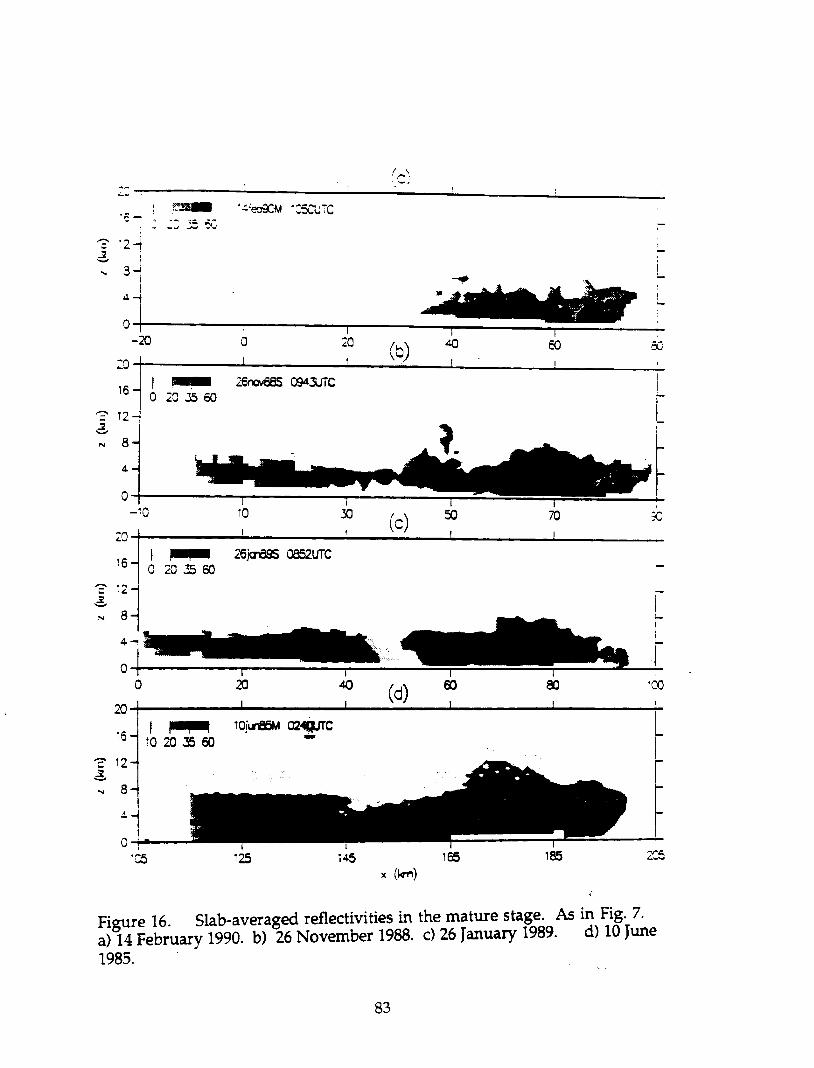
16

....., 12 .2 '-"

"" 8

4.

}'3l!_

= '::.35 5C

I \ , ro ' --;-

L

I

L L

201.-==----=~---!......-~-....L-----L---.-:.. f ,... 26jCTB95 Cl852UTC

16

,... .... ... "

.6 ,.,. 8

16

? 12 ~ ... 8

a 20.35 60

I~ 10 203560

O~--

·co

10j~ 02-GJTC -

125 165 185

Figure 16. Slab-averaged reflectivities in the mature stage. As in Fig. 7. a) 14 February 1990. b) 26 November 1988. c) 26 January 1989. d) 10 June

1985.

83

/_\

,-j

.: -------...:..--.-~----..!.--~----, I

i -'J""i

I .--.. I

6 ""

;::,

:; , I

'0 20 .:D 40 :D 6J :;Q

I, ) \W

'c:

',j,fetJ9JM lCSOUTC

J4-----~-----------J

x (i<m)

Figure 17, Slab-averaged velocities and vorticity in the mature stage. As in Fig. 8. a) 26 November 1988. b) 14 February 1990. c) 10 June 1985. d) 26 January 1989,

84

.-/

.~------~------------~----------------~----~-------·: . ..r55M :2':':L.-:

I I

,....

OJ, I

6 I

"

5

0 '.30 140 150 100

.=:

26;CTC9S C852UiC

'0

---6

" 5

Figure 17 (continued).

170

(d)

85

" -_ ..

'8)

~·r ---~~-t ... ,! " .. , .... -­

>.

t , ,... ..

\ I ,

'00 '2J)J

-,~ , ---:. .'1.

t··- · ....

...... ""\ .. ~

.:0 .

I , ~,

.-" .....:' ________ ~_l...__.!...

-l • 20 J5 it)

.-~ ~i-----.;.----.!.-........:...~~=-

:j -I

-1 ~ -t---;,-~I----;I;-----=r=:::::::....~.:::.:.::..+- -120 +--~-_r_-_r_-~:.:::.::....,...:::=..:::...;.... - ~ 20 -BO -J.() .J 4() aJ 120 -120 -8J -40 0 4()

x (4'1'1) x (10m)

(c)

'20 -t1---'----'----'-----l--L' -~

~~ ! ~ 120 -t--~-.....L--.....L--......I.... ___ ....J' ___ --_I 80

10 2C ~ .;0 I

!

-4Q

..-..

-:§. 0

40

·411 .r' I L

-120 I i ! i -'~ -BO -40 0

X (~)

i 00

o

Figure 18. Horizontal reflectivity maps in the mature stage. As in Fig. 6. a) 26 November 1988. b) 26 January 1989. c) 14 February 1990. . d) 5 December 1989.

86

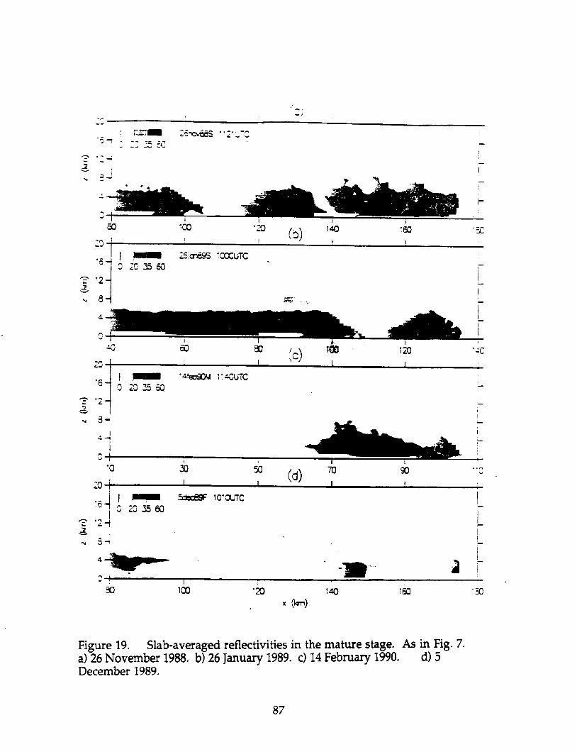
'-~---:----~----.:.....----:...--~ r:z_ :: __ :c

-I

140 .:c

25:cr89S 1ca:urC

~.

8;-----==r=======;~-........;

-'"'1 _ ..... ~.J. 0' ~ _ 20 J5 50

,6 " 8-

C1--------~,----------r-------~~~~~~~ '0 )) 50 (d) 70 .. ('\

"

L ~ L

L : 1 i

-. i

j

120 140 1&'J '30 x (m,)

Figure 19. Slab-averaged. reflectivities in the mature stage. As in Fig. 7. a) 26 November 1988. b) 26 January 1989. c) 14 February 1990. d) 5 December 1989.

87

'~~--------------~----------------~----~-----I • -:':~~M __ 1_ .....

~~II'1

I ') ~a

.:~----~----~--~----~----~----~----~-----5cec89F ~ c: a... TC

---

C~--~~----------------~--~~~~--~~--, ----~~~----110 120 140 15J ~70

x (km)

Figure 20. Slab-averaged velocities and vorticity in the mature stage. As in Fig. 8, except horizontal scale is different. a) 26 November 1989. b) 26 January 1989. c) 14 February 1990. d) 5 December 1989.

88

.:;

':>:--a.'E.CS 4, . ..J ....

I i

........ '~1

~ ....

5

0 'CO 110

'S -26j<T89S tCXX)UTC

'0

-J, N

::

Figure 20 (continued).

-~

:20 1.lJ 140

(' ) \0

110

89

-400- -

1&l

120 1.l)

--'00

--~ ~ -~

08

Figure 21. Integration volume for vorticity equation, adapted from Rotunno et al. (1988). Plus and minus signs enclosed in circular arrow symbols denote vorticity, streamlines are bold arrows, and the boundary of the cold pool is shown with the conventional cold front symbol. The integration region is the smaller rectangle, with FU denoting flux at the upper face, and FL denoting flux at the left face. a) RKW assumptions; b) Relaxed assumptions as described in the text.

90

a

--N

'i:

. I I

I - .. ~ E I ~

I I

! - i N

2 ....

--.lC :0 60

C .

I - I .:.~

E 1 ~ -

N 2

'-.'0-J

I

50 a:l 70 20

X ( k m ) Figure 22. Left- and upper-face vorticity transport (described in text) from the 26 November 1988 DUNDEE squall line. Times are a) 1830 LT, b) 1851 LT, and c) 1913 LT. The lightest gray shading corresponds to values between 50 and -50 m2s-2, medium gray represents magnitudes between 50 and 200 m2s·2, and darkest gray greater than 200 m2s·2. The heavy curve represents the vorticity minimum. The arrow represents the gust front position. In a), the heavy box is a hypothetical integration volume (see text).

91

Figure 23. The three-region model. Region i is a sloping zone of constant vorticity with slope a.. It is embedded in region "b" (below) characterized by constant vorticity and depth Zjl as well as region "a" (above) which is also characterized by constant vorticity and depth ZrZj. The bold outline denotes the region over which circulation is determined, as described in the text.

92

26jan89s 0.0 100 r:-:-------------.

t.l 60 a.

q " 50 '\11

~ ·1.0 10.3 ->

'i ')." ,~~ ~o. (;'D.

~ V . 0 00_. 40 _

01 CD 15 'g j ·1.5 10.3

5 30 i 11:1 0

(j5

20 < .2.0 10')

M 10 .2.5 10.3 •

100 150 200 2Se time (min)

26novU. 0.0 10° r:-r. •• ---------------.60

.3.0 10'3 ............................................ '--'--........................ L...i... .......... ....J a o so 100 150 200 250

timelninl

lOjun85a 0.0 10° r-"""'!r"-----------. 60

'. · . · . · . M d 0 50

40 _ r 'a

30 -J WI

20

'tr 10

0 a so 100 1 so 200 250

time (min)

(a)

(b)

(c)

Figure 24. Observed slopes and average vorticity in the interior of six squall lines. Dashed lines with open squares are average vorticity. Solid lines with filled circles are the slope of the zone of maximum negative vorticity in degrees (scale at right). The symbol "M" represents the Mature stage, with vertical bars denoting the approximate beginning and end of that stage. a) 26 January 1989. b) 26 November 1988. c) 10 June 1985. d) 7 February 1990. e) 5 December 1989. f) 18 November 1989.

93

7fab90m 0.010° 60

-5.0 10 4 I M I ? 50 - . ' II>

~ :.. - -1.010.3 c 40 0 >

q~ 0" .. 0" 0 9 -1.510 3 r-

Q>

iii '. : 0 30 ~ '. .c 5 0·0 !. (d) Q> 5! > -2.0 10.3 I-« 20 '"

-2.510.3 10

-3.0 10.3 I 0

0 50 100 150 200 250 lime (min)

Sdec89l

0.0 10° 60

-5.0 10.4 . D 0- a " 50

-~ -1.0 10.3 po. 40 0 0 p.od Q> > '0 - - - -0 - - - 0 ~ 0 -1.5 10.3. 30 I § <e) == '" Q>

-2.0 10.3 > 20 «:

-2.510.3 a : '0

10

-3.010.30 50 100 150 200 25cP lime (min)

18n09"~ 0.0 10° 60

-5.0 10.4 50

~ -1.010.3 40 _ > 0

0 oC:! C III

-1.5 10-3 ,0- ~ !!. c 30 I !!

'= (I) • '" ~ -2_010-3 20

-2.5 10-3 M

10

-3.010-3

0 50 100 150 200 259 time(lTin)

Figure 24 (continued).

94

a 6 \ \ \ "- "- \ \ \ \ \ , , , \ \ \ \. \, "- \ \ \ \ , , , \ \ "- \. '- "- , \ \ \ \ , , '4 \ '\ "- "- "" - T

, \ \ \ \

\, "- "- "- '" - ~ T .\ \ \ \

" "- " "- "'- - ." r 1 , , , "- '- "- " ........ / r , , Q ,

" ...... '" ......... -.... - /' I , , ... - - - -"- ..... ...... ""~--.~ /' / T ... - - - - - -.... -. ........... -.... • ......... /' ,

.. - -- .. ~ ~ ... - ... ~

20 .lJ 40 50

b 'E "\ \, "- "" " -

, \ \ , "- '- '-""'" ..... , , \ , , t .... "- '" "", ...... ... r i , , . t ..... '- ....... ~, ....... ,

T l t r "- '- ....... " .................. - ;I' I T T 1 , .... ...... ...... ....... "'- ......... -- -- I , r r , .... ..... ...... ............................ -.-,,? I , t -2 .... ..... ...... .................. -...~".,;t ./ I I "' ~ .... -. ....... -....- ... ,.-.,/ ,,? /

... - ---~- ., :.0 ~~.,.... ;I'

--., ~ ~ ~ ~---+ - , - - - -0

20 .lJ 40 50

C ~

" ,,-,~ ....... - , f l T r I I " ,

....... "'-" ................. ." , r I I ,

" ,

...... .............. , ............... - , 1 ~ , I ,

" ,

" ........................... ~- /' ! I I ;' , , ...... "" ........................... - ".;t I ! ! ,

" , .-

..... ............................ ~-....-. ./ I / / ,;- "" .-..... ...... ....... ~ .......... -.....-..--..~ /' / I , ,;- , ~ -. ..................... -......-. ........... /' ./ / ,;- , - ..... - -.. -.....---r- oJ ~ ~//' ,,? ;'

- - - - -..--. ~ ~ ~ ...................... ~ - - - -- ., ~ ~ .. ~ .... - ... .t)

20 JO 40 50

Figure 25. The effects of inflow strength on the velocity distribution. Vectors spanning one grid unit in either dimension represent 20 ms-1. All plots are for lower shear of 4xlo-3s-1, zero upper shear, and Region i slope of 1.0 (a = 45 "). Surface velocities at the right boundary (inflow strengths) are a) -18 ms· I, b) -12 ms-1, and c) -6 ms-I .

95

a 6 j 1 ) \ ,,> , 'S os "" , • • .. 'i" {\ \ \ \ \

\ \ ~ ~, \ \ ~ \ \

4

2.

\ \ \ \ \

" ,

\\~"--..,. i \\\ \ \ \ ~ ~ ~ r i ~ \ \ '- '- ~'-..'-.- ~ f i' \ , \''-."",,'-.~- ..... / r it ..... "''''''----....'''-.~-)' T r t '> " -.... ......... ~--..- ........ I r r ... , ................ '"-..;~-.-" /' I r .. .... --...~~~~/)' , - ---...~ ) )~........ " - -., ) .~ ....

o I i) 20 .l) 40

b 6 1 ) I) 5 ' I, I , , , < , , (

4-

2-

\ \ \, \ \ \ \ '- ~ ... \ \ \ '- , .... \ \ \", ..... \ \ " ..... ..... ..... - ... , 1 .... " " ...... - I r ... '> , ...... - / I ................ - .... /

\ \ \ \ , ! I

.... ___ -/' I

--.--.~."... .",.

-.. ---. ---+ ~

, , , \

o Iii W .l) 40

c 6 I

4-

...

2

... " " ... ... " " ... , , ... ...

, , , ... , ... ...

...

\ ,

50

... , ,

~

I-

50

o Iii i W .l) 40 ~

Figure 26. The effects of the strength of Region i vorticity on the velocity distribution. Vectors spanning one grid unit in either dimension represent 20 ms-1. All plots are for lower shear of 2x1O-3s-1, zero upper shear, and inflow strength of 12 ms-1. Minimum Region i vorticities are a) -1x10-2s-1, b) -6x10-3s-1, and c) -2xlO-3s-1.

96

5

4

2

a

: : ~ ~ ~~:} 1 \ \ \ '" ~~~I r T ,

1 I '

I ,

. , \ ",'~~--.y" r T

., ''' ...... '-......... ~~l ", , , " ...................... ~--...,..../' !"

, ......................... ~~/! f' • , " ................ -.::::; 'S ... ;'# /' / ' ,

, ........ ~ ; '9 ,..,,/ I I

... - .. '4 , ):~ .. /' '

> )s:)~

O~-------r------~------~------~--------~~~~~------~ 20 40 60 70

b

""" ..... ~~~ ......... -\"\'" , 5 • , , ... " ............................... ~ ~ \ \ \ \ , I

, , , ........... '" ................ ~ , \ \ \ , I I

4 .,' , .... ' ...................... -..:;--r .... ' \, I I •

................. _ ....... ~-...;;--~ .... ," I'

3 • .. ........ - _ ...... -, ~ .. • ..... , T I I

............ --- ... ., ., .. "' T , ' 2

....... ___ ~. .. v, , I

..... ....... -- .... » •• / , , .. - ... - ____ ._J-tI~ ...... / , I-

1.' .... '----O~------~------~------~------~----~~_+~+_~------4_

20 40 60 70

c 6~----__ ~I--------~I--------~J--------~J--------~1--------~I------~

5- ..... ~ ............................ - . " " " " .... "" '\ ,

4- ....... -- .... -. ......................... --- '" , " '" , , , , -- - ... - -- -- .... -..-..-..--..-..-. ~ , , " , , ,

3- - - ........................... -..-.-.~ ~ \ , , \ ..

2-___ -._. .... .-..-...-.e", ....

, - --- ... ~-----.-- .... '\ - - - - ~ . ------ ... - ... .-..... --,,-

0~--------~1---------~1--------1~------~1---------T-1------~1~-------4-20 ~ 40 ~ 60 70 ~ 90

Figure 27. The effects of the slope of Region i on the velocity distribution. Vectors spanning one grid unit in either dimension represent 20 ms-I . All plots are for lower shear of 2xIO-3s-1, zero upper shear, and inflow strength of 12 ms-I . a) a=4S", b) a=27", and c) a=I4".

97

800

700

C':l- 600 (I)

N 500 g x ~ 400 ~ "0 300 f-

200

100

0 0 0.5 1.5 2 2.5

(l

Figure 28. Total flux for conditions of zero upper shear, 4xl0-3s-1 lower shear, and vorticity zone strength -lxl0-2s-1.

4000

C':l- 3500 (I)

Ng 3000 x ~ 2500 B - 2000 ... Cl) "0 0 1500 -c c::: 0 1000 (.) Cl)

(J)

500

0 0 500 1000 1500 2000 2500 3000 3500 4000

max flux from relaxation solution (m2s'2)

Figure 29. Total flux computed using Eq. 18 (ordinate) vs. the total flux computed using the relaxation solution. The sloping solid line represents a ratio of 1:1.

98

'-Q) 0.C01

a. a. ::> E -O.CO' Q)

:c E

«-O.COJ

ClCXl3 0.cx:J3 0.012

Ambient Lower Shear

Figure 30. The value of the denominator of Eq. 18 for a range of shear values. Shears units are s-l.

99

0.15

0.1

0.05 -~

0 I r.J) C) Q) '0 -0.05 -::: ~

-0.1

-0.15

-0.2

-0.25

5 10 15 20 25 30 35 slope(deg)

Figure 31. Examples of solutions to Eq. 18. Values on the abscissa are the slope of the Region i vorticity zone in degrees. Values on the ordinate are the tilting rate from Eq. 18, in degrees per second. See text for additional explanation.

100

a DCAPE = -500 m2s-2

0.003 0.CXl3 0.012

Figure 32. Equilibrium slopes (<I, degrees) as a function of upper and lower shear strength, for cold pool strengths of a) -500 m2s-2, b) -1000 m2s-2, and c) -1500 m2s-2.

101

0.003 O.C03 0.Oi2

Ambient lower shear (s-1)

Figure 33. a) Average magnitudes of cold pool strength (m2s·2) that are associated with steady storms, as a function of upper and lower shear. b) As in a), but range of magnitudes of cold pools strengths (m2s·2) where steady storms are possible.

102

...: -- ,/

<' " /

<:-/ ,

; / /',

" ./ :=: :-----'---'--..:....r---"'-.,..-"?~~

:~' , "',(/ / ~::- ',/' ,', /

.' "< e::-' / <.<,/ )<~ s:: / ',(

20000

15000

f., 10000 ]

5000

( e,

.....

'<

~:

0_25 -20 -IS -10 -5 0 5 10 15 20 2S

0.25

~~ -56W.·~ 0

\ & -0.25 \ ! ;0 ..aom2s-2 ....

-0.5

-0.75 -200rnz.·Z\\ \

\

~, ~ \

-1 5 10 15 20 25 30 35

510pe(089)

a

b

C

Figure 34. Pre-storm environment and tilting solutions for 26 January 1989. a) skew-T log-P diagram (temperature in degrees C) from 0000 UTC, with moist adiabats at 340, 350, and 360K; b) storm-relative line-normal environmental flow; c) tilting rate (degs-1) as a function of slope (l for lower and upper estimates of cold pool strength (labelled in graph).

103

a

.'

/

".

" 2::- /""-. ---------~----~------~~~----

--0

b :~ ~----------------------------~

15000

sooo

o ~----~~------------------~ -25 -20 -15 -10 -5 0 5 10 15 20 25 relalive u (ms· 1)

c 0.25

0

-'"

-0.25 -670m~-2 01 = So.

,:: -0.5

-0.75 ~-'2~5-2 -1

5 10 15 20 25 30 35 SIOI)e(Cleg)

Figure 35. As in Fig. 34, but for 26 November 1988.

104

- - ,

/ ,/

/ . ,\

-::-/ 'XC /

--0 -:;: -2:

a

J:

b :~ r-----------------------~

15000

< \

5000

o~~--~~------~----~ ·30 -25 ·20 -IS -10 -5 0 5 10 15 20 relative u (ms' I)

c 0,25

o

'1-0.25

-0.5

-0.75

-1

5 10 15 20 25 30 35 slope (deg)

Figure 36. As in Fig. 34, but for 10 June 1985.

105

a

·_oJ 3:

b ::0000

15000

-~ 10000 ]

5000

0 ·15 ·20 ·15 ·10 ·5 0 5 10 15 20 25

relative u (ms :)

C 0.'5

0.1 / 0.05 ~

- 0 '0 al ·0.05 ~

i= ·0.'

·0.'5

·0.2

·0.25

5 10 15 20 25 30 35 slope(deg)

Figure 37. As in Fig. 34, but for 7 February 1990.

106

-~ ~

/

"

(

/ '/ (

'<

/' ,

,

/ -' .',

a

"

~ ' ..... / ---:----~~--~~~~~~~~

-~o -3: -2:

b ::0000

15000

10000

5000

o~ __ ~--~--~~~~~~ -25 -20 -15 -10 -5 0 5 10 15 20 25

relative u (ms'l)

c 0,25

o

'I -0,25

-0.5

-0.75

-1

5 10 15 20 25 30 35 slope (deg)

Figure 38. As in Fig. 34, but for 18 November 1989.

107

a

'.

<

" ~----~--~----------~~~~--~

a::-

- -'J J:

b :oooor-----------------------~

• 15000

/

'. .§.

~10000

~ ]

5000

~ 0 -25 -20 -15 -to -5 0 5 10 15 20 25

relative u (rns· l )

C 0.25

0

1-0.25

i§ -0.5

-0.75

-1

5 10 1S 20 2S 30 3S slope (deg)

Figure 39. As in Fig. 34, but for 5 December 1989.

108

2.5 10.1

0.0 10°

- ·2.5 10.1 in en Q)

:9-::: ·5.0 10.1 i=

-7.510.1

-1.0 10° 5 10 15 20 25 30 35

slope(deg)

Figure 40. Graph of tilting rate versus slope for mid-latitude environments. The curves are for DCAPE of -100, -500, -1000, and -1500 m2s-2.

0.25

o

.- -0.25 en C) -soo m2s·2 Q)

:E.. - -0.5 ~

-0.75

-1

5 10 15 20 25 30 35 slope(deg)

Figure 41. Graph of tilting rate (degs-1 on ordinate) versus slope for the environmental conditions associated with the 23 June 1981 COPT 81 squall line. Cold pool strengths are indicated on the graph.

109

0.15

0.1

0.05

?- 0 , (J) C) Q)

-0.05 "0 --i= -0.1

-0.15

-0.2

-0.25 5 10 15

I ,

20 slope (deg)

- -,.,.

25

, 0 '()

h 5 ~ --10 '

30 35

Figure 42. Graph of tilting rate versus slope for the five shear conditions examined in Thorpe et al. (1982).

0.15

0.1

0.05 --- 0 , (J)

en Q)

:2. -0 05 = . i=

-0.1

-0.15

-0.2

-0.25 5 10 15 20 25 30 35

Figure 43. Graph of tilting rate versus slope for four shear configurations including the optimal shear determined by RKW, using the RKW units of ms-1per2500 m.

110

0.CXl3

- 0.004 -~ '- ~ CU <b 0.C02 .c en ...

f,f ) <b Q. a. ~ 0 E .I'f <b :c E

10iunl( <: -o.C02 Tropics f I

Chong

-O.C()4. +

-o.C02 o.em O.COO 0.012

Ambient lower shear (s-1)

Figure 44. As in Fig. 33, but with various individual cases and climatological parameter spaces superimposed. The sloped lines represent fixed DCAPE in units of m2s-2. See text for additional details.

111

A Formative stage

B Intensifying stage

Figure 45. Conceptual model of squall line evolution. Heavy lines represent the cloud boundary and thin lines are streamlines of the line-normal flow. The sign of the vorticity is indicated with "+" and "_". The square inset represents a low-level horizontal depiction of the reflectivity. The arrow associated with the label "w" represents relative updraft magnitude in a slab average, and with "c" a relative propagation speed.

112

C Mature stage ..

c

D Dissipating stage

- - - - - -

Figure 45 continued.

113

I

REFERENCES

Bluestein, H. B., and M. H. Jain, 1985: Formation of mesoscale lines of

precipitation: severe squall lines in Oklahoma during the spring. J.

Atmos. Sci., 42, 1711-1732.

Charba, J., 1974: Application of the gravity current model to analysis of squall­

line gust fronts. Mon. Wea. Rev., 102, 140-156.

Chalon, J. P., G. Jaubert, F. Roux, and J. P. Lafore, 1988: The west African

squall line observed on 23 June 1981 during COPT 81: Mesoscale

structure and transports. J. Atmos. Sci., 45,2744-2763.

Chong, M., P. Amayenc, G. Scialom, and J. Testud, 1987: A tropical squall line

observed during COPT 81 experiment in West Africa. Part I:

Kinematic structure inferred from dual-Doppler data. Mon. Wea. Rev.., 115, 670-694.

Cotton, W. R, and R A. Anthes, 1989: Storm and cloud dynamics. Academic

Press, 883 pp.

Cunning, J. B., 1986: The Oklahoma-Kansas Preliminary Regional Experiment

for STORM-Central. Bull. Amer. Meteor. Soc., 67, 1478-1486.

114

Emanuel, K. A., 1986: Some dynamical aspects of precipitating convection. J.

Atmos. Sci., 43, 2183-2198.

Emanuel, K. A., 1989: Dynamical theories of tropical convection. Aust. Met.

Mag., 37, 3-10.

Fovell, R G., and Y. Ogura, 1988: Numerical simulation of a midlatitude

squall line in two dimensions. Mon. Wea. Rev., 45, 3846-3879.

Hane, C. E., 1986: Extratropical squall lines and rainbands. Mesoscale

Meteorology and Forecasting. P. S. Ray, Ed., American Meteorological

Society, pp. 359-389.

Houze, R A., S. A. Rutledge, M. I. Biggerstaff, and B. F. Smull, 1989:

Interpretation of Doppler weather radar displays of midlatitude

mesoscale convective systems. Bull. Amer. Met. Soc., 70, 608-619.

Houze, R A" B. F. Smull, and P. Dodge, 1990: Mesoscale organization of

springtime rainstorms in Oklahoma. Mon. Wea. Rev., 118, 613-654.

Hoxit, L. R, C. F. Chappell, and J. M. Fritsch" 1976: Formation of mesolows or

pressure troughs in advance of cumulonimbus clouds. Mon. Wea. Rev.,

104, 1419-1428.

115

Johns, R. H., and W. D. Hirt,1983: The derecho- A severe weather producing

convective system. Preprints, 13th Conf. on Severe Local Storms, Tulsa,

Oklahoma, Amer. Meteor. Soc., 178-181.

Johnson, R. H., and P. J. Hamilton, 1988: The relationship of surface pressure

features to precipitation and airflow structure of an intense midlatitude

squall line. Mon. Wea. Rev., 116, 1444-1472.

Kessinger, C. J., P. S. Ray, and C. E. Hane, 1987: The Oklahoma squall line of

19 May 1977. Part I: A multiple Doppler analysis of convective and

stratiform structure. ]. Atmos. Sci., 44, 2840-2864.

Lafore, J.-P., and M. W. Moncrieff, 1989: A numerical investigation of the .

convective and stratiform regions of tropical squall lines. ]. Atmos. Sci.,

46, 521-544.

Lafore, J.-P., and M. W. Moncrieff, 1990: Reply. J. Atmos. Sci., 47, 1034-1035.

Leary, C. A, and R. A. Houze, 1979: The structure and evolution of

convection in a tropical cloud duster. J. Atmos. Sci., 36, 437-457.

Lemone, M. A., 1983: Momentum transport by a line of cumulonimbus. ,.

Atmos. Sci., 40, 1815-1834.

116

Maddox, R. A., 1980: Mesoscale convective complexes. Bull. Amer. Meteor.

Soc., 61, 1374-1387.

McAnelly, R. L, and W. R. Cotton, 1989: Precipitation life cycle of mesoscale

convective complexes over the central United States. Mon. Wea. Rev.,

117, 784-808.

Ogura, Y., and M.-T. Liou, 1980: The structure of a midlatitude squall line: A

case study. ]. Atmos. Sci., 37, 553-567.

Rotunno, R., J. B. Klemp and M. L. Weisman, 1988: A theory for strong, long­

lived squall lines. ]. Atmos. Sci., 45, 463-485.

Rotunno, R., J. B. Klemp and M. L. Weisman, 1990: Comments on "A

numerical investigation of the organization and interaction of the

convective and stratiform regions of tropical squall lines." J. Atmos.

50.,47,1031-1033.

Roux, F., 1988: The west African squall line observed on 23 June 1981 during

COPT 81: Kinematics and thermodynamics of the convective region. J.

Atmos. Sci., 45, 406-426.

117

,.

. '. '~\. .".~.,. .,........ :

Rut .... jL· .. , 1991: Middle Latitude and ttopical mesoscale convective .• f~j,···:· "",,~, Geophys., Supplement (April 1991), 88-97 . . ,:.1;?i~~~ ~'<:... ~. "

Rutledge, S. A., R. A. Houze, M. L Biggerstaff, and T. Matejka, 1988: The

Oklahoma-Kansas mesoscale convective system of 10-11 June 1985:

PrecipitatiOn structure and single-Doppler radar analysis. Mon. Wea.

ReD., 116, 1409-1430.

Rutledge, S. A., E. R. Williams, and T. D. Keenan, 1992: The Down Under

Doppler and Electricity Experiment (DUNDEE): Overview and ".;, r::;'

preliminary results. Bull. Amer. Meteor. Soc., in press. __ ,.

i<

Schlesinger, R. E., 1975: A three-dimension8I numerical model of an isolated ,

deep convective cloud: Preliminary results. J. Atmos. Sci., 32, 934-957.

Schmidt, J. M., and W. R. Cotton, 1989: A High Plains squall line associated .

wi. severe surface winds. J. Atmos. Sci., 46, 281-302. .... ~

.-_ ... _,1983: The dynamical structure of squall-line type

Smull, B. F., and R. A. Houze, 1985: A midlatitude squall line with a ttailing

region Of stratiform rain: Radar and satellite observations. Mon. Wea.

Rev., 113, 117-133.

118

Smull, B. F., and R A. Houze, 1987: Rear inflow in squall lines with trailing

stratiform precipitation. Mon. Wea. Rev., 115, 2869-2889.

Smull, B. F., and R A. Houze, 1987: Dual-Doppler radar analysis of a

midlatitude squall line with a trailing region of stratiform rain. J.

Atmos. Sci., 44, 2128-2148.

Thorpe, A. J., M. J. Miller, and M. W. Moncrieff, 1982: Two-dimensional

convection in non-constant shear: A model of mid-latitude squall

lines. Quart. J. R. Met. Soc., 108, 739-762.

Zhang, D.-L., and K. Gao, 1989: Numerical simulation of an intense squall

line during 10-11 June 1985 PRE-STORM. Part II: Rear inflow, surface

pressure perturbations and stratiform precipitation. Mon. Wea. Rev.,

117,2067-2094.

Zipser, E. J., 1977: Mesoscale and convective-scale downdrafts as distinct

components of squall-line structure. Mon. Wea. Rev., 105, 1568-1589.

119