6

Observations and initial fields

‘. . . the icy layers of the upper atmosphere contain conundrums enoughto be worthy of humanity’s greatest efforts . . . ’ . (Hergesell, 1905)

We have seen in the last chapter how Richardson constructed a complete algorithmfor integrating the equations of motion and, in the following one, we will studythe application of his method to an actual weather situation. To do that, initialconditions are required, and we describe in this chapter the means of obtainingthem. We outline the emergence of aerology, the study of the upper atmosphere.We describe an ingenious instrument for making aerological observations Then weconsider some results of Bjerknes’ ‘diagnostic programme’. Finally, we discussthe preparation of the initial fields for the numerical forecast.

6.1 Aerological observations

During the 19th century, measurements of atmospheric conditions at the Earth’ssurface were made on a regular basis, and daily surface weather maps were issuedby several meteorological institutes. Observations at elevated locations were muchmore difficult to obtain. A number of mountain stations were established towardsthe end of the century: Mt. Washington in 1870, Pike’s Peak in 1873, Pic du Midiin 1886, Fujiyama in 1898 and Zugspitze in 1900 (Khrgian, 1959). However, cli-matological conditions at mountain stations have particular characteristics. Whatwas desirable was an investigation of conditions in the free atmosphere. Severalintrepid balloonists ascended with instruments to measure the vertical structure ofthe atmosphere. James Glaisher, of the Royal Observatory in Greenwich, madenumerous ascents in the 1860’s to measure the variations of temperature and hu-midity with height. Such explorations were both expensive and dangerous; indeed,there were a number of fatalities. The credit for initiating systematic observationsof the upper air goes to Lawrence Rotch of Blue Hill Observatory, Boston, who

95

96 Observations and initial fields

around 1895, started the method of attaching self-recording instruments to kites.Kites and tethered balloons had a limited vertical range, and the steel piano-wireused to control them occasionally snapped, with serious consequences.1

Sounding balloons, which carried self-registering instruments aloft as they roseby natural buoyancy, were proposed by George Besancon and Gustave Hermite (anephew of the renowned mathematician, Charles Hermite) as a powerful, practicaltechnique for exploring the higher reaches of the atmosphere. These balloons weretracked by two theodolites, separated by a baseline of 1 km or more. Balloonslaunched at night were equipped with a small light to render them visible. Thewind speed and direction at each level could be deduced from the azimuth andelevation bearings of the theodolites. A large specially-designed slide-rule wasused for the calculations, and the winds were available in near ‘real-time’. Pilotballoons were small balloons without any instruments attached. They were namedfor the aviators who launched them prior to take-off to see how the winds aloftwere blowing. For the temperature and humidity, the recording instrument had tobe recovered. This normally took at least several days. Such data were clearly ofno relevance for operational weather prediction, but would prove hugely beneficialto researchers.

In addition to the government-funded activities, several aerological observato-ries were established by enthusiasts. Thus, the observatories at Blue Hill, Bostonand at Trappes, Paris were run by Lawrence Rotch and Teisserenc de Bort respec-tively, using their own financial resources. Aeronautical pioneers also contributedto the advancement of this emerging science.2 The first instrumented balloon as-cent was carried out by Gustave Hermite on September, 17th, 1892, using a waxedpaper balloon. Constant volume balloons halt their ascent when they reach theirlevel of neutral buoyancy. Around 1900, Richard Assmann, Director of the RoyalPrussian Observatory in Berlin, revolutionised the sounding technique when heintroduced rubber balloons. These expand with height, maintaining an approxi-mately constant rate of ascent. Assuming this rate to be known, the position can bedetermined by means of a single theodolite. These expanding balloons never reacha position of equilibrium, but continue to rise until they burst. They enable mea-surements to be made at heights up to 15 or 20 km. They are reliable and relativelyinexpensive and are still in use today. The method of upper air observation usingsounding balloons came into widespread use from this time. It was now possible

1 In one notorious incident an array of kites, launched by Teisserenc de Bort, broke loose and drifted acrossParis trailing 7 km of wire. They stopped a steamer and a train and disrupted telegraphic communicationswith Rennes on the day when the results of the Dreyfus court-martial in that city were anxiously awaited(Ohring, 1964).

2 Bjerknes (1910) summarized the symbiosis between aviation and aerology: ‘The development of aeronauticswill make these [aerological] observations not only possible, but also necessary.’

6.1 Aerological observations 97

Fig. 6.1. International Meteorological Conference, Paris, 1896 (from Shaw, 1932).

to launch balloons simultaneously from several locations, raising the possibility ofsynoptic aerology (Nebeker, 1995).

At the Conference of the International Meteorological Organization in Paris in1896 (see Fig. 6.1), a Commission for Scientific Aeronautics (ICSA) was estab-lished. Hugo Hergesell, Director of the Meteorological Institute of Strasbourg,was appointed President of the Commission. Hergesell was actively involved inupper air observations. He was also a consummate diplomat, and succeeded inovercoming the rivalry between the French and German scientists and establish-ing excellent international collaboration. The tasks of the Commission were toco-ordinate and regulate upper air research in Europe, to establish standards and toorganize simultaneous observations of the free atmosphere on ‘International Aero-logical Days’. Hergesell published a series of reports of the ICSA Conferences. Healso published, between 1901 and 1912, some 22 volumes of data acquired duringthe Aerological Days. The first such experiment was on 13/14 November, 1896,with remarkable results, which Shaw would, much later, refer to as ‘the most sur-prising discovery in the whole history of meteorology’ (Shaw, 1932, p. 225). Thesonde launched from Paris showed an isothermal layer above 12 km. This was the

98 Observations and initial fields

first indication of the stratosphere, but the measurements were discounted as erro-neous and it took several years before the existence of the tropopause and strato-sphere were firmly established, independently by Teisserenc de Bort and RichardAssmann. For an interesting account of the events surrounding the discovery of thetropopause, see Hoinka, 1997.

Upper air observations were made only intermittently, typically for one or a fewdays each month, as agreed by the countries participating in the work of the ICSA.European aerological stations active at this time included Aachen, Bath, Berlin,Copenhagen, De Bilt, Guadalajara, Hamburg, Kontcheiv, Lindenberg, Milan, Mu-nich, Pavia, Pavlovsk, Strasbourg, Trappes, Uccle, Vienna and Zurich. The Inter-national Aerological Days, or ‘Balloon Days’, were normally on the first Thursdayof each month. In three months of each year the adjacent Wednesday and Fridaywere added, giving three consecutive days and, once a year, six consecutive days,the ‘international week’. The co-operation came to a sudden end with the FirstWorld War. Although the radiosonde was invented in 1927, it was not until afterthe Second World War that a real synoptic upper air network was established inEurope.

6.2 Dines’ meteorograph

William Henry Dines (Fig. 6.2) was a master in the design and construction of me-teorological instruments. He was active on the Wind-Force Committee that wasset up following the Tay Bridge disaster. A train fell into the river when the bridgewas blown down in a storm in December, 1879, with the loss of over one hundredlives. This provided a strong incentive for the development of instruments capableof measuring the wind accurately. One result was Dines’ pressure-tube anemome-ter, an ingenious construction that gives a continuous record of the wind speed anddirection, with detailed reading of gusts and lulls. Dines also expended consider-able energy investigating solar and terrestrial radiation, and undertook some moregeneral studies of atmospheric structure. However, his main contributions were tothe study of the upper atmosphere. Although it was not until 1908 that regular aero-logical observations began in England, Dines began his investigatons of observingtechniques some years earlier. Shortly after Sir Napier Shaw took charge of theMet Office in 1900, he encouraged Dines to undertake observational studies of theupper air. Dines had exceptional flair in designing meteorological instruments, andhis meteorograph, which we will describe now, was a masterpiece of economy andefficiency (Dines 1909).

Registering balloons measured pressure, temperature and humidity during theirascent and recorded the values by means of an instrument called a meteorograph.Analysis of the values was dependent upon this instrument being found after its de-

6.2 Dines’ meteorograph 99

Fig. 6.2. W. H. Dines (1855–1927). From Collected Scientific Papers of William HenryDines, Royal Meteorological Society, 1931.

scent by parachute. To encourage finders to return the device, a notice was attachedto the instrument, offering a reward (see Fig. 6.3). According to Dines (1919) ‘it isastonishing how many are returned; the [European] continental stations do not losemore than one out of ten, but in England many fall in the sea and the loss reaches30 or 40 per cent.’

Wind speeds and directions at various heights were deduced by following thecourse of the ascending balloon. Obviously this became impossible once the bal-loon entered cloud. But these observations were available promptly, whereas thepressure and temperature data were obtained only when the instrument was foundand returned after its descent. As Dines wrote (1919), ‘The mere sending up ofa registering instrument attached to a balloon does not necessarily mean a goodobservation. The instrument may never be found, the clock may stop, the pen may

100 Observations and initial fields

Fig. 6.3. Label attached to meteorographs of the Met Office, offering a five shilling rewardfor return of the instrument (from Dines, 1912).

not write, the finder may efface the record; there are many possibilities of failure.’On 20 May 1910, for example, the observation for Vienna comprised only winds;no pressures or temperatures were available, the registering balloon being recordedas bis heute noch nicht gefunden (Hergesell, 1913). It is unlikely to be found now.

The instruments were not standardised, different systems being used in differentcountries. In the French and German instruments, records were made on smokedpaper secured to a drum which was turned by a clock. The instruments weighedabout 1 kg and required a ballon of diameter 2 m to carry them. The meteorographdesigned by Dines was of elegant simplicity, inexpensive to make and weighingabout an ounce (30 g). Its cost was only £1, in comparison to £15 or £20 forinstruments used in other countries. It carried no clock but recorded temperatureas a function of pressure. In favourable circumstances the instrument could becarried by a small balloon to a height of 20 km.

A diagram of Dines’ meteorograph is presented in Figure 6.4. The frame iscut from a single piece of metal, the end

�being turned down at right angles to

allow it to open and close like a pair of scissors as the aneroid box � expands orcontracts with changing pressure. One side of the frame carries two steel points(pens) � and � and on the other there is a small square metal plate the size of apostage stamp on which they etch marks as they move. Pen � , attached to bar �records the pressure. The lever ���� carrying pen � is free to pivot about � ; asthe temperature falls, the strip of German silver contracts, so point � moves

6.2 Dines’ meteorograph 101

Fig. 6.4. Dines meteorograph for upper air soundings. (A) Photograph of instrument show-ing the aneroid box. (B) Schematic diagram indicating the operating principle. (C) Mete-orogram, showing scratches on a small metal plate. [Dines, 1909, 1912].

downward and pen � upward. With uniform temperature, a decrease of pressurecauses two parallel scratches on the plate, whereas a change of temperature causesa change in the distance between the scratches. After retrieval, the small plateis removed from the instrument and examined under a microscope. The distancebetween the marks indicates the temperature as a function of the pressure. A thirdelement to measure humidity can easily be added. It is similar to the temperatureelement but the expanding metal strip is replaced by strands of hair, the lengthof which is sensitive to the relative humidity of the air. The right-hand panel inFig. 6.4 is a meteorogram produced by Dines’ instrument.

The height may be obtained by means of the hydrostatic relationship so that, for

102 Observations and initial fields

a column between pressures ��� and ��� , the thickness is

����� ��� � � �� ���� ������� � ��� ����� � ���

where �� is the mean temperature of the column. This can easily be evaluatedusing special graph-paper. A detailed example was given in Dines (1909). He alsogave an estimate of the accuracy of his meteorograph: the error in temperature isgenerally less than � � C; the pressure error less than 10 mm Hg (about 13 hPa).This means that at 10 km the height error may be up to 400 m, and at 20 km upto about 1500 m. These are quite large errors and cause considerable uncertainty,particularly for the analysis at higher levels.

6.3 The Leipzig charts

The forecast made by Richardson was based on ‘one of the most complete sets ofobservations on record’ (WPNP, p. 181). At the time he made this forecast (be-tween 1916 and 1918) a comprehensive set of analyses of atmospheric conditionshad become available. The two volumes of ‘Dynamic Meteorology and Hydrog-raphy’, by Vilhelm Bjerknes and various collaborators, had appeared in 1910 and1911. The second volume was accompanied by a large atlas in which the firstisobaric analyses were published. These maps were the first attempt to analysesynoptic conditions in the upper atmosphere. On becoming Director of the newGeophysical Institute in Leipzig, Bjerknes began a consolidated and systematicdiagnostic analysis of the aerological data. The first of the series of ‘Synoptis-che Darstellungen atmospharischer Zustande’ (the synoptic representation of theatmospheric conditions) was published in 1913. This related to January 6, 1910.Further analyses, also relating to the year 1910, appeared over the following twoyears. The issue of primary interest to us is Bjerknes, 1914b.

Bjerknes’ analyses consisted of sets of charts of atmospheric conditions at tenstandard pressure levels from 100 hPa to 1000 hPa. These charts were pro-duced to high-quality, in large format ( !#"%$�"'& cm), covering Europe at a scaleof 1:10,000,000. There were normally fourteen charts for each observation time(see Table 6.1). The compilation of the charts was performed for the most part byBjerknes’ assistant, Robert Wenger. They were the first comprehensive aerologi-cal analyses ever published. They enabled Bjerknes to study the three-dimensionalevolution of atmospheric conditions, and to test his prognostic methods that werebased on graphical techniques (Bjerknes, et al., 1910, 1911). He was convincedthat, ultimately, charts such as these would be the basis for a rational forecastingscheme. In this he was correct, although perhaps not in the manner he envisaged:

6.3 The Leipzig charts 103

Table 6.1. Analysed charts in Synoptische Darstellungen atmospharischerZustande. Jahrgang 1910, Heft 3 (Bjerknes, et al, 1914b). The Roman numerals

in column 2 are the level indicators used by Bjerknes. For 0700, 20 May, 1910 the100 mb analysis is missing, due to lack of sufficient observational data at this

level.

Chart Level Content

1 Sea Level Pressure (mm Hg) and Temperature ( � C)2 Surface streamlines and isotachs (m/s)3 Cloud cover and precipitation4 X 1000mb Height and 1000-900 Relative Topography5 IX 900mb Height and 900-800 Relative Topography6 VIII 800mb Height and 800-700 Relative Topography7 VII 700mb Height and 700-600 Relative Topography8 VI 600mb Height and 600-500 Relative Topography9 V 500mb Height and 500-400 Relative Topography

10 IV 400mb Height and 400-300 Relative Topography11 III 300mb Height and 300-200 Relative Topography12 II 200mb Height and 200-100 Relative Topography13 I 100mb Height14 Tropopause Height

the charts provided Richardson with the data required for his arithmetical forecast-ing procedure.

The ‘international days’ were normally on the first Thursday of each month. Innormal circumstances, there would have been a balloon day on Thursday, 5th May,1910. It is interesting that the observational period for May 1910 was postponedto coincide with the passage of Halley’s comet. There was some speculation thatthe comet might cause a detectable response in the atmospheric conditions, andwhat would now be called an ‘intensive observing period’ was undertaken. Forexample, on 19 May, a series of hourly ascents over a period of twenty-four hourswas carried out at Manchester to ascertain the diurnal variation of temperature.The comet passed between the Earth and the Sun on 18th May; as the tail curvedslightly backwards, the passage of the Earth through it occurred a little later, onthe 20th, the day chosed by Richardson (Lancaster-Browne, 1985). Comets arepopularly thought to portend dramatic events; one may say that on this occasion a

104 Observations and initial fields

Table 6.2. Upper Air Observations from registering balloons, pilot balloons andkites for 0700 UTC, 20 May, 1910. For the full reports, see Hergesell, 1913.

Location Minimum Maximum Temperature Instrumentof Pressure Height ( � C)Launch (mm Hg) (metres)

Aachen 360 6,000 -15.3 Registering BalloonBergen 9,600 Pilot BalloonChristiania 8,100 Pilot BalloonCopenhagen 12,020 Pilot BalloonFriedrichshaven 460 4,110 -3.9 Kite BalloonHamburg 195 10,410 -50.1 Registering BalloonLindenberg 299 7,420 -25.9 Registering BalloonMunich 186 10,600 -55.6 Registering BalloonNizhni-Olchedaev 632 1,580 5.9 Captive Balloon/KitePavia 108 13,850 -63.7 Registering BalloonPavlovsk 132 12,560 -46.5 Registering BalloonPyrton Hill 69 17,600 -45.5 Registering BalloonStrasbourg 85 15,530 -54.2 Registering BalloonTenerife 4,710 Pilot BalloonUccle 91 14,980 -57.8 Registering BalloonVienna 19,700 Reg. Balloon (lost)Zurich 118 13,450 -47.7 Registering Balloon

comet was associated with an event of great significance for meteorology, thoughnot due to its having any direct influence on the atmosphere.

The date and time chosen by Richardson for his initial data was 20 May, 1910,0700 UTC. During the three day observing period there ascended altogether 73registering balloons (33 of which included wind observations), 35 kite and captiveballoons, 81 pilot balloons and four manned balloons. Aerological observationswere reported for the following locations: Aachen, Bergen, Christiania, Copen-hagen, De Bilt, Ekaterinburg, Friedrichshafen, Hamburg, HMS Dinara (near Pola),Lindenberg, Manchester, Munich, Nizhni-Olchedaev, Omsk, Pavia, Pavlovsk, Pe-tersfield, Puy de Dome, Pyrton Hill, Strasbourg, Stuttgart, Tenerife, Trappes, Uc-cle, Vienna, Vigne di Valle, Zurich and, from outside Europe, Apia, Blue Hill andMt. Weather. The stations of most relevance for Richardson’s forecast are indicatedin Fig. 6.9 on page 109 below. The soundings and reports of upper level winds overwestern Europe for 0700 on 20th May, 1910 are given in Table 6.2. The full compi-

6.3 The Leipzig charts 105

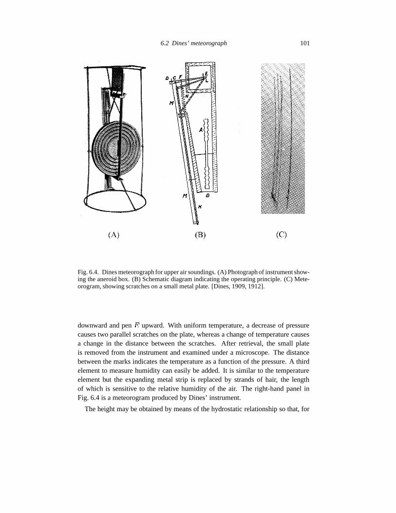
Fig. 6.5. Bjerknes’ analysis of sea level pressure (solid lines, mm Hg) and surface temper-ature (dashed lines, � C) for 0700 UTC on May 20, 1910.

lation of observations occupies more than one hundred pages in Hergesell (1913).The observations are tabulated in a compressed form in Bjerknes, 1914b.

The weather conditions during the period 18–20 May, 1910 were summarized inHergesell’s publication:

The distribution of atmospheric pressure was very irregular on the days of the as-cents and, consequently, there were frequent thunderstorms, especially in west-ern and central Europe. A cyclone moved northwards from the Bay of Biscaywhile a weak minimum drifted westwards from the Adriatic, gradually inten-sifying and an anti-cyclone over Scandanavia gradually increased in strength(Hergesell, 1913).

The Leipzig publication contains 13 charts for the time in question: sea-levelpressure and surface temperature, surface streamlines and isotachs, cloud and pre-cipitation, geopotential heights and thicknesses for nine standard levels at 100 hPaintervals from 1000 hPa to 200 hPa, and tropopause height (see Table 6.1). The

106 Observations and initial fields

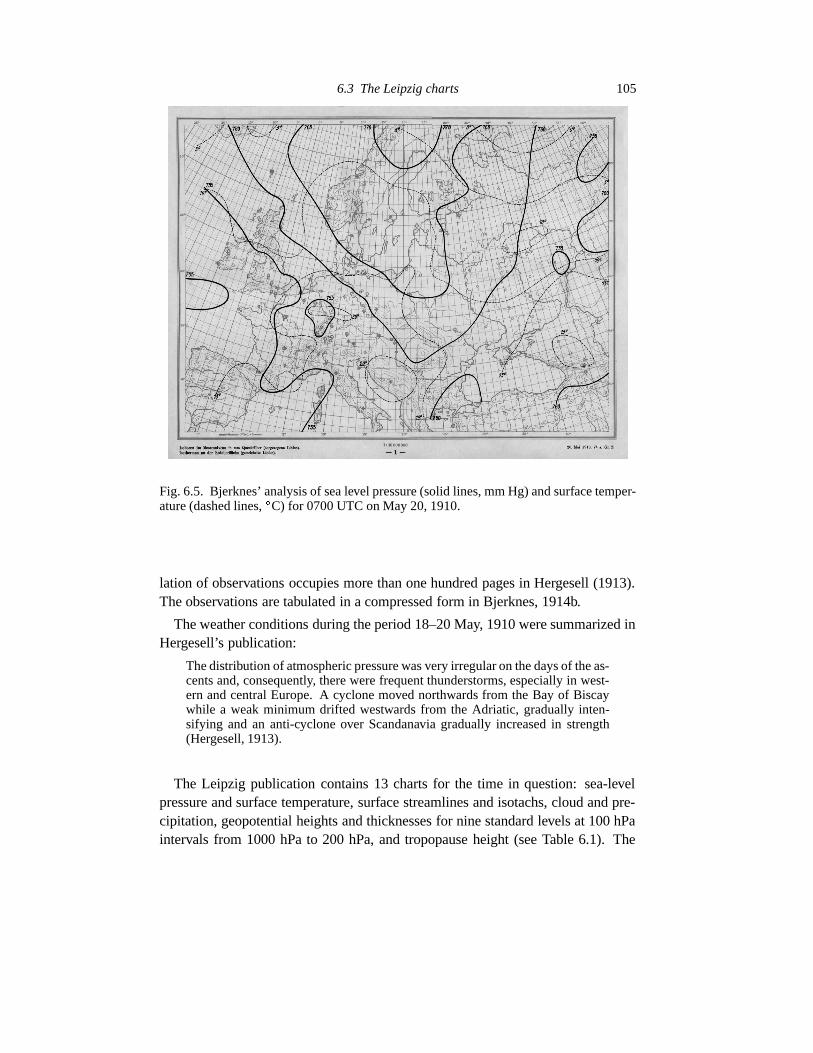
Fig. 6.6. Bjerknes’ analysis of 500 hPa height (heavy lines, dam) and 500–400 hPa relativetopography (light lines, dam) for 0700 UTC on May 20, 1910.

sea-level pressure and surface temperature chart is reproduced in Fig. 6.5 and the500 hPa height in Fig. 6.6.3

Data coverage was reasonable at the surface; for the upper levels, the number ofobservations is seriously limited, leaving great uncertainty over much of the areaof interest. In a commentary on the analysis, Wenger wrote that there was no causeto doubt the reliability of any of the ascents. He further commented that ‘the goodagreement of the wind vectors with the topography of the main isobaric levels’ wasa ground for confidence in the pressure analysis. Thus, he explicitly recognized thatthe flow in the free atmosphere should be close to geostrophic balance.

Conditions at the surface are also shown in the analysis of the Met Office(Fig. 6.7). The left panel shows the sea level pressure at 0700 UTC. It is in generalagreement with Bjerknes’ analysis (Fig. 6.5). There is high pressure over Scan-danavia and low pressure over Biscay, associated with a generally south-easterlydrift over Germany and France. The right panel of Fig. 6.7 shows the sea-levelpressure at 1800 UTC on the same day. There is little change in the overall pattern

3 The full series of charts is available online at http://maths.ucd.ie/ � plynch/Dream/Leipzig-Charts.html.

6.3 The Leipzig charts 107

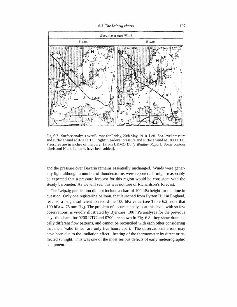
Fig. 6.7. Surface analysis over Europe for Friday, 20th May, 1910. Left: Sea-level pressureand surface wind at 0700 UTC. Right: Sea-level pressure and surface wind at 1800 UTC.Pressures are in inches of mercury. [From UKMO Daily Weather Report. Some contourlabels and H and L marks have been added].

and the pressure over Bavaria remains essentially unchanged. Winds were gener-ally light although a number of thunderstorms were reported. It might reasonablybe expected that a pressure forecast for this region would be consistent with thesteady barometer. As we will see, this was not true of Richardson’s forecast.

The Leipzig publication did not include a chart of 100 hPa height for the time inquestion. Only one registering balloon, that launched from Pyrton Hill in England,reached a height sufficient to record the 100 hPa value (see Table 6.2; note that100 hPa � 75 mm Hg). The problem of accurate analysis at this level, with so fewobservations, is vividly illustrated by Bjerknes’ 100 hPa analyses for the previousday: the charts for 0200 UTC and 0700 are shown in Fig. 6.8; they show dramati-cally different flow patterns, and cannot be reconciled with each other consideringthat their ‘valid times’ are only five hours apart. The observational errors mayhave been due to the ‘radiation effect’, heating of the thermometer by direct or re-flected sunlight. This was one of the most serious defects of early meteorographicequipment.

108 Observations and initial fields

(a) Valid time 0200 UTC (b) Valid time 0700 UTC

Fig. 6.8. Bjerknes’ height analyses at 100 hPa at two times on 19 May, 1910. (a) Analysisat 0200 UTC. (b) Analysis at 0700 UTC. Note that only five hours separate the two analysistimes.

6.4 Preparation of the initial fields

6.4.1 Richardson’s analysis

Using the most complete set of observations available to him, Richardson derivedthe values of the prognostic parameters at a small number of grid points in centralEurope. The values he obtained were presented in his ‘Table of Initial Distribu-tion’ (WPNP, p. 185). Richardson chose to divide the atmosphere into five layers,centered approximately at pressures 900, 700, 500, 300 and 100 hPa (see Fig 5.1on page 89). He divided each layer into boxes and assumed that the value of a vari-able in each box could be represented by its value at the central point. The boxeswere separated by

��� � ��� & � in longitude and��� ��� �� � in latitude. Richardson

tabulated his initial values for a selection of points over central Europe. The areais shown on a map on page 184 of WPNP (reproduced as Fig. 6.9).

In 9/1 of WPNP, Richardson describes the various steps he took in preparinghis initial data. He prepared the mass and wind analyses independently (today, thisis called univariate analysis). The data were obtained from the compilations ofHergesell and the aerological charts of Bjerknes. The pressure values were com-puted from heights read directly from Bjerknes’ charts. The momentum valueswere computed using the observations tabulated by Hergesell, followed by visualinterpolation or extrapolation to the grid points. Richardson recognized the un-certainty of this procedure: ‘It makes one wish that pilot balloon stations couldbe arranged in rectangular order, alternating with stations for registering balloons

6.4 Preparation of the initial fields 109

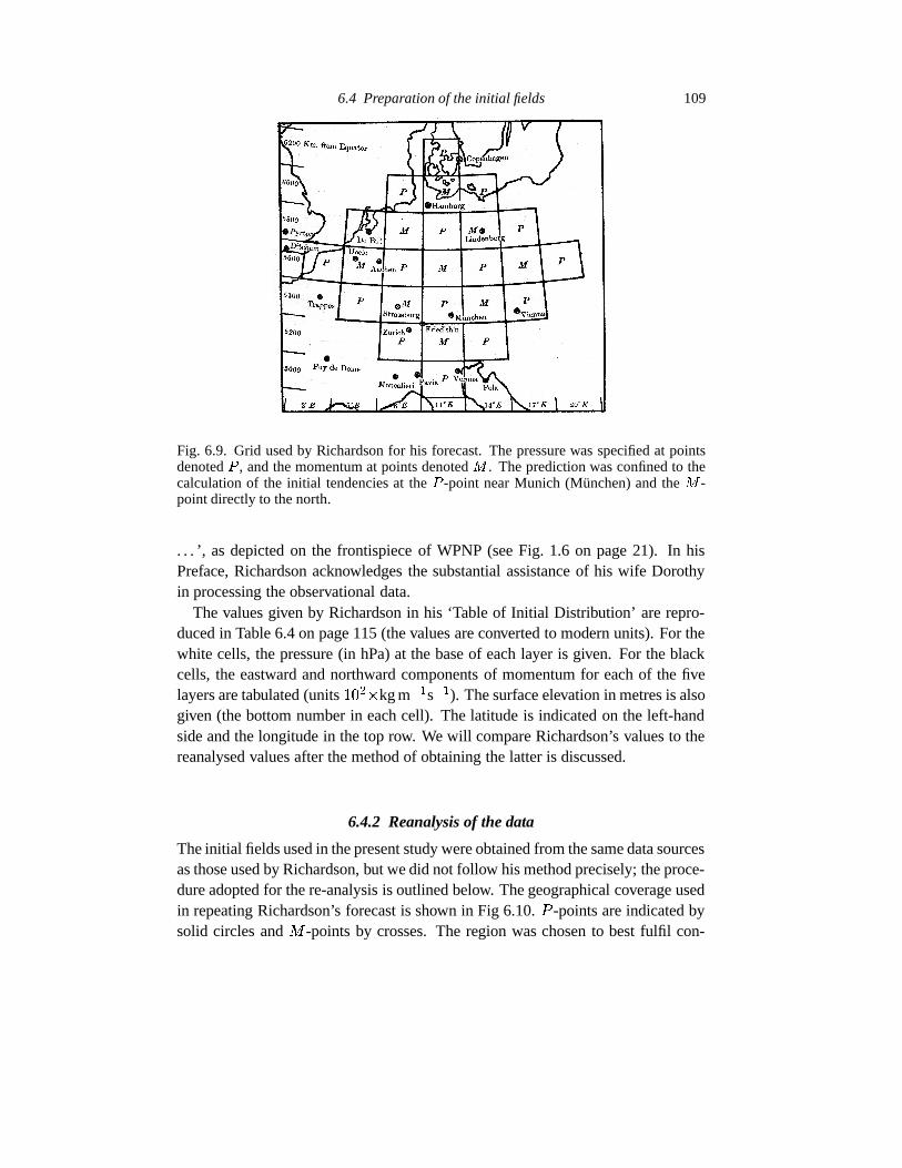
Fig. 6.9. Grid used by Richardson for his forecast. The pressure was specified at pointsdenoted � , and the momentum at points denoted � . The prediction was confined to thecalculation of the initial tendencies at the � -point near Munich (Munchen) and the � -point directly to the north.

. . . ’, as depicted on the frontispiece of WPNP (see Fig. 1.6 on page 21). In hisPreface, Richardson acknowledges the substantial assistance of his wife Dorothyin processing the observational data.

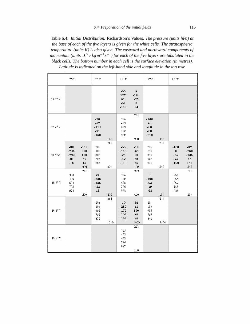
The values given by Richardson in his ‘Table of Initial Distribution’ are repro-duced in Table 6.4 on page 115 (the values are converted to modern units). For thewhite cells, the pressure (in hPa) at the base of each layer is given. For the blackcells, the eastward and northward components of momentum for each of the fivelayers are tabulated (units

� & � $ kg m � � s � � ). The surface elevation in metres is alsogiven (the bottom number in each cell). The latitude is indicated on the left-handside and the longitude in the top row. We will compare Richardson’s values to thereanalysed values after the method of obtaining the latter is discussed.

6.4.2 Reanalysis of the data

The initial fields used in the present study were obtained from the same data sourcesas those used by Richardson, but we did not follow his method precisely; the proce-dure adopted for the re-analysis is outlined below. The geographical coverage usedin repeating Richardson’s forecast is shown in Fig 6.10. � -points are indicated bysolid circles and -points by crosses. The region was chosen to best fulfil con-

110 Observations and initial fields

Fig. 6.10. The geographical coverage used in repeating and extending Richardson’s fore-cast. � -points are indicated by spots and � -points by crosses. The � -point and � -pointfor which Richardson calculated his tendencies are shown by encircled marks.

flicting requirements: That it be as large as possible; that data coverage over thearea be adequate; and that the points used by Richardson be located centrally in theregion. The absence of observations precluded the extension of the region beyondthat shown. The � -point and -point for which Richardson calculated his ten-dencies are shown by encircled marks. In order that the geostrophic relationshipshould not be allowed to dominate the choice of values, the pressure and velocityanalyses were performed separately (and by two different people).

The mass field

The initial pressure fields at level interfaces were derived from Bjerknes’ charts ofgeopotential height at 200, 400, 600 and 800 hPa (his charts 6, 8, 10 and 12). Atransparent sheet marked with the grid-points was super-imposed on each chart andthe height at each point read off. Each level ��� corresponds to a standard height

� �with temperature

� � . Conversion from height�

to pressure � was made using thesimple formula

� � ��� � � � � � � ������

6.4 Preparation of the initial fields 111

where ��� � � ��� � . The geodynamic heights� � of the standard levels were 1.959,

4.113, 7.048 and 11.543 km (see WPNP, p. 181). The standard temperatures� � at

the surface and interfaces were � ��� ����� � ����� � � ����� � �� ��� ����� � � & ��� .Sea-level pressure values were extracted in the same way as heights, from Bjerk-

nes’ Chart #1 (Fig. 6.5). His values, in mm Hg, were converted to hectopascals bymultiplication by 4/3. Then the surface pressure ��� was calculated from

��� � �������� � ���

���� � ��� �"!

where�

is orographic height at the point in question, � �#��� is the sea-level pressureand standard values

�$� � � �&% and �� & � &�&'! � %(' � � were used for the surface

temperature and vertical lapse-rate.In the absence of a 100 hPa chart in the Leipzig collection for the time in ques-

tion, the 100 hPa topography and 200-100 hPa thickness were analysed using thefew available observations and a generous allowance of imagination. The thicknessvalues

� � �� � �)� � � � �)� were then used to calculate the stratospheric temperature,

� � �� � �� � � � � � �

where �� � ��� &+*�, � and� � � � &�&+*�, � are the mean pressure and pressure thick-

ness of the layer. Considering the uncertainties, the values were surprisingly closeto those obtained by Richardson (see below).

The momentum field

The initial values of momenta for each of the five layers are required. These werederived from the wind velocities at the intermediate levels 100, 300, 500, 700 and900 hPa. The observed wind speeds and directions for each level, as compiled byHergesell and also tabulated in Bjerknes’ publication, were plotted on charts uponwhich isotachs and isogons (lines of constant wind speed and direction) were thendrawn by hand. The grid-point values of speed and direction were then read off.It was necessary to exercise a degree of imagination as the observational cover-age was so limited, particularly over the Iberian peninsula. The wind values wereconverted to components - and . and the layer momenta / and 0 were defined by

/ �21 - � � �� . � 0 ��1 . � � �� . (6.1)

where� � is the pressure across the layer (obtained in the pressure analysis).

Orography

The atlas included with Part II of Dynamic Meteorology and Hydrography (Bjerk-nes, et al., 1911) contains two charts of orographic height, one ‘moderately ideal-

112 Observations and initial fields

Fig. 6.11. Bjerknes’ chart of ‘greatly idealized’ orography. Contours are at 200 m (dotted),500 m (dashed), 1000 m (solid) and 2000 m (solid). (Plate XXIX in Bjerknes, et al., 1911).

ized’ and one ‘greatly idealized’. Values of surface height at each grid-point wereread off from the latter chart (Bjerknes, et al., 1911, Plate XXIX), which is re-produced in Fig. 6.11. As Richardson remarks, ‘At some points there is a largeuncertainty as to the appropriate value of

�; for example in Switzerland the uncer-

tainty amounts to several hundred metres.’

6.4.3 Tables of initial data

The pressure, temperature and momentum values, at a selection of points in thecentre of the domain, resulting from the reanalysis, are given in Table 6.3. Thecorresponding values obtained and used by Richardson, extracted from his ‘Tableof Initial Distribution’(WPNP, p. 185), are reproduced in Table 6.4. The orographicheights are also indicated (bottom number in each block). To facilitate comparison,the orography values used by Richardson were also used in the reanalysis.

There is reasonable agreement between the pressure and stratospheric tempera-ture values in the two tables. In general, pressure differences are within one or twohectopascals. There is a notable exception at the point

� " ��� !�� � � � � &���� � , wherethe old and new values differ by 10 hPa. We will see below that Richardson’svalue at this point is suspect. A similar table of initial values appears in Platzman(1967) in which two surface pressures at " !����� � are question-marked. In fact, it

6.4 Preparation of the initial fields 113

is the orographic heights in Platzman’s table that are incorrectly transcribed fromWPNP.

Comparing the momenta in Tables 6.3 and 6.4, we see much more significantdiscrepancies. Although the overall flow suggested by the momenta is similar ineach case, point values are radically different from each other, with variations aslarge as the values themselves and occasional differences of sign. These dissimilar-ities arise partly from the different analysis procedures used, but mainly from thelarge margin of error involved in the interpolation from the very few observationsto the grid-points.

The investigation of the comparison between the old and new momentum values,using modern techniques of objective analysis, is an attractive possibility, but itwill not be explored here.4 Instead, in the forecast in Chapter 7, we have simplyreplaced the reanalysed values of all fields by Richardson’s original values at the(few) gridpoints where the latter are available. The values in Table 6.4 are thusthe initial values for both Richardson’s forecast and the forecasts described in thefollowing chapters. In consequence of this, the calculated tendencies at the centralpoints of the domain will be found to be essentially the same as those obtained byRichardson.

4 Recently, ECMWF has completed a reanalysis back to 1957 (see � 11.4 below). Perhaps some day ‘in the dimfuture’, they will reach back to 1910.

114 Observations and initial fields

Table 6.3. Initial Distribution: Reanalysed Values. The pressure (units hPa) atthe base of each of the five layers is given for the white cells. The stratospherictemperature (units K) is also given. The eastward and northward components ofmomentum (units

� & � $ kg m � � s � � ) for each of the five layers are tabulated in theblack cells. The bottom number in each cell is the surface elevation (in metres).

Latitude is indicated on the left-hand side and longitude in the top row.

� � ��� ��� ���

����

����

��� �����

��� ��������������

����� ���� �������� ���

���� ��� ����� �����

����� ���� �������� ���������� ����

���� ���� ����� ����� �������� ���� ����

���� ��� ��� ���� ����� �����

���� ���� ���� ��������� ���� ���������� �� �� �����

���� ����� ����� ����� �������� ����

���� ��������� �����

�� �� ���� ��� ����� ���� ���� ����

������ ������� �����������

���������

����� ��������������

�����

� � � � �

���

���

���

���

���

���

� � � � �

�

�

�

�

�

�

����� � ����!����� ����"�"� � !#�

� $#% �� ���#� !#�

� ��� �&�('����)�! �*%�$����)�) �����#%����)�' ����'������'�' ����!#�

����%�' ����! ������' ����!�� �*����� �&�+��!� ��$�� ����) � ����! � )�! �*���#% �&�+��)� ��"#$ ��%�" � ���#� ����! �*��'�' �*��)��������! $($ ����$�$ %�) �&�+��" �� !�! '+� �����#% %�) �*�(%�' !(�

����'�$ ����)#�� �#%�' � ����'� �#��� ����",%����)#� ������$� ��� �&!+�

� ����! ��!� ��!�$ �����%�� ��%���-"#' ��"� )�� )�!

6.4 Preparation of the initial fields 115

Table 6.4. Initial Distribution. Richardson’s Values. The pressure (units hPa) atthe base of each of the five layers is given for the white cells. The stratospherictemperature (units K) is also given. The eastward and northward components ofmomentum (units

� & � $ kg m � � s � � ) for each of the five layers are tabulated in theblack cells. The bottom number in each cell is the surface elevation (in metres).

Latitude is indicated on the left-hand side and longitude in the top row.

� � ��� ��� ���

���

��� �

��������

����� ��������������

���� ��� �������� �����

���� �������� ����

���� ���� ��������� ���������� �����

��� ��� ��� ��� �������� ����� �����

���� ���� �������� ���� ����

����� ���� ���� ��������� ����� ���������� ����� �����

��� ��� ��� ��� �������� �����

���� �������� ����

����� ���� ��������� ���������� �����

����� ����� ����������

��������

���� ��������������

���

� � � � �

���

���

���

���

���

���

� � � � �

�

�

�

�

�

�

����� !�"$# � !�%�&

! � " ��� ! %

� !�' &

� #�% � ! � %

�(� " &$%

� !)!�& �(� %

� '$! �(� %

� ! � % � "$!�'

�(* % � !�!�% ����� � ! � !�%)% �(* "

� "�& � * %)% � !�& � �(� " % � " � %

� ")" * ! �) � ' � "�' �(�)� � ! *)�� '$! # ��� " �� � " � & � ! ! � � !)!�% ��� � !�')% ! � %

"$# %

�(* " � ! ���� ! *)� � ' ��(*)* � !�'& �(�)�

��� % %

� " % &+!

� !)# � ! � %

� !�% � %

� ! �)� &,%