1

Observed Climate Change and the NegligibleGlobal Effect of Greenhouse-gas Emission

Limits in the State of Alabama

www.scienceandpublicpolicy.org

[202] 288-5699

2

Summary for Policy Makers 3

Observed climate change in Alabama 4Annual temperature: 4Seasonal temperatures: 5Precipitation 6Drought 7Crop Yields: 8Sea Level Rise: 8Extreme events - Hurricanes: 11Vector-borne Diseases: 18

Impacts of climate-mitigation measures 22

in the state of Alabama

Obama’s Cap & Trade Proposal 26

Impact of the EU Actions – Other nations 28

Conclusion 30

Costs of Federal Legislation 30State Pension funds at risk? 31

Alabama Scientists Reject UN’s GlobalWarming Claims 33

Appendix: Recent Global Temperatures 34

References 35

Table of Contents

3

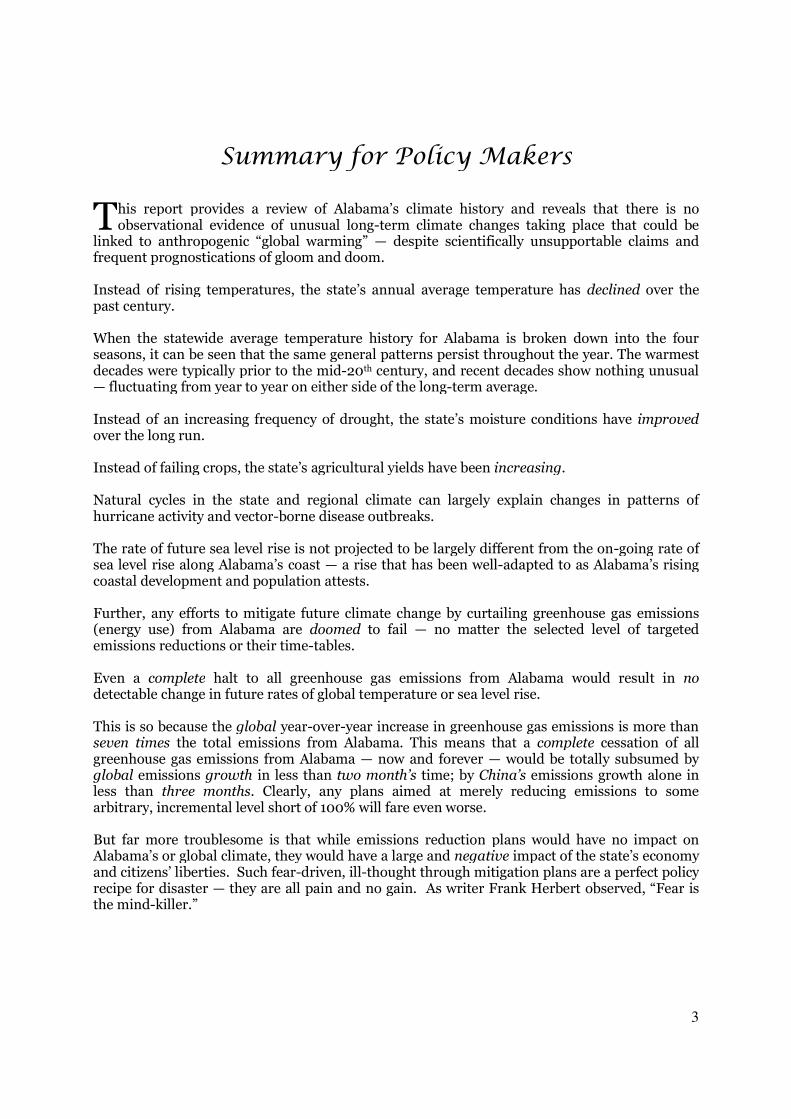
Summary for Policy Makers

his report provides a review of Alabama’s climate history and reveals that there is noobservational evidence of unusual long-term climate changes taking place that could be

linked to anthropogenic “global warming” — despite scientifically unsupportable claims andfrequent prognostications of gloom and doom.

Instead of rising temperatures, the state’s annual average temperature has declined over thepast century.

When the statewide average temperature history for Alabama is broken down into the fourseasons, it can be seen that the same general patterns persist throughout the year. The warmestdecades were typically prior to the mid-20th century, and recent decades show nothing unusual— fluctuating from year to year on either side of the long-term average.

Instead of an increasing frequency of drought, the state’s moisture conditions have improvedover the long run.

Instead of failing crops, the state’s agricultural yields have been increasing.

Natural cycles in the state and regional climate can largely explain changes in patterns ofhurricane activity and vector-borne disease outbreaks.

The rate of future sea level rise is not projected to be largely different from the on-going rate ofsea level rise along Alabama’s coast — a rise that has been well-adapted to as Alabama’s risingcoastal development and population attests.

Further, any efforts to mitigate future climate change by curtailing greenhouse gas emissions(energy use) from Alabama are doomed to fail — no matter the selected level of targetedemissions reductions or their time-tables.

Even a complete halt to all greenhouse gas emissions from Alabama would result in nodetectable change in future rates of global temperature or sea level rise.

This is so because the global year-over-year increase in greenhouse gas emissions is more thanseven times the total emissions from Alabama. This means that a complete cessation of allgreenhouse gas emissions from Alabama — now and forever — would be totally subsumed byglobal emissions growth in less than two month’s time; by China’s emissions growth alone inless than three months. Clearly, any plans aimed at merely reducing emissions to somearbitrary, incremental level short of 100% will fare even worse.

But far more troublesome is that while emissions reduction plans would have no impact onAlabama’s or global climate, they would have a large and negative impact of the state’s economyand citizens’ liberties. Such fear-driven, ill-thought through mitigation plans are a perfect policyrecipe for disaster — they are all pain and no gain. As writer Frank Herbert observed, “Fear isthe mind-killer.”

T

4

Observed climate change in Alabama

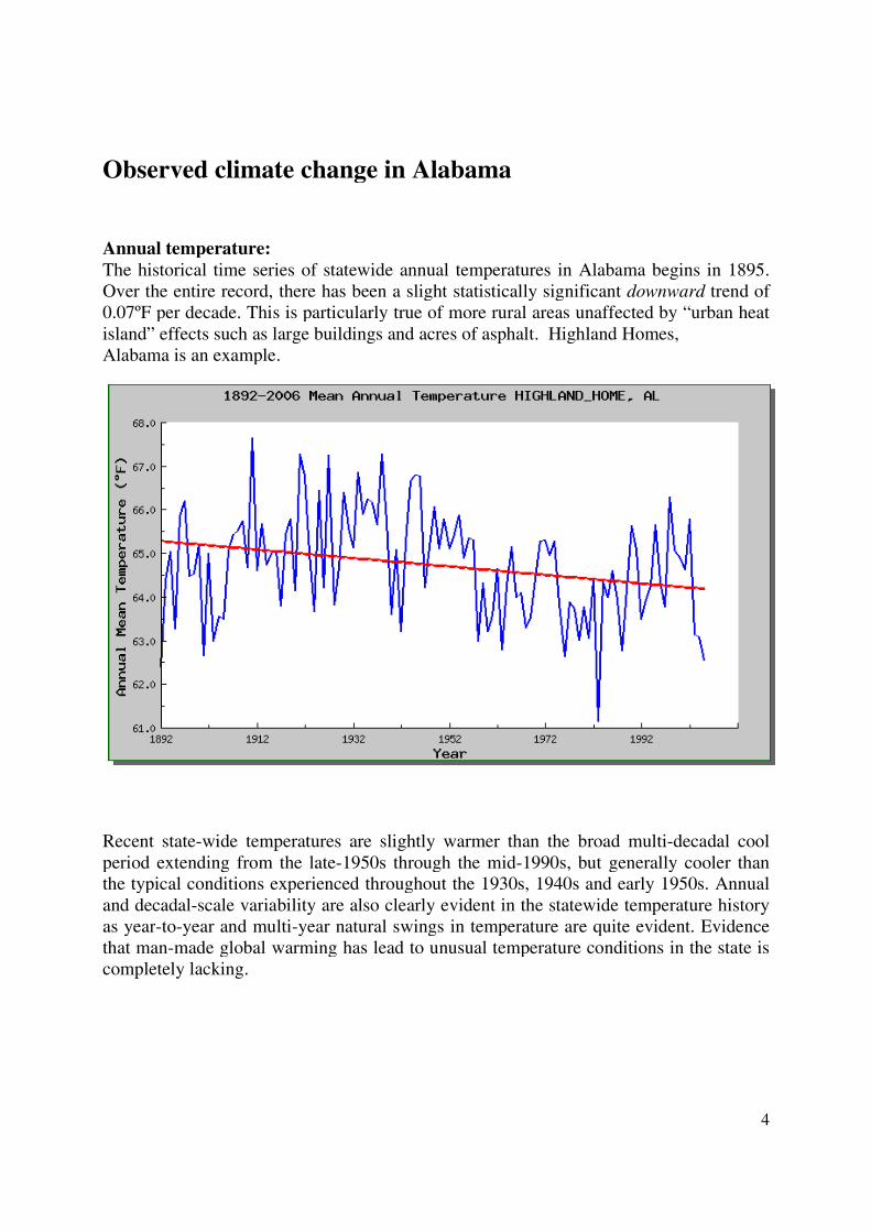
Annual temperature:The historical time series of statewide annual temperatures in Alabama begins in 1895.Over the entire record, there has been a slight statistically significant downward trend of0.07ºF per decade. This is particularly true of more rural areas unaffected by “urban heatisland” effects such as large buildings and acres of asphalt. Highland Homes,Alabama is an example.

Recent state-wide temperatures are slightly warmer than the broad multi-decadal coolperiod extending from the late-1950s through the mid-1990s, but generally cooler thanthe typical conditions experienced throughout the 1930s, 1940s and early 1950s. Annualand decadal-scale variability are also clearly evident in the statewide temperature historyas year-to-year and multi-year natural swings in temperature are quite evident. Evidencethat man-made global warming has lead to unusual temperature conditions in the state iscompletely lacking.

5

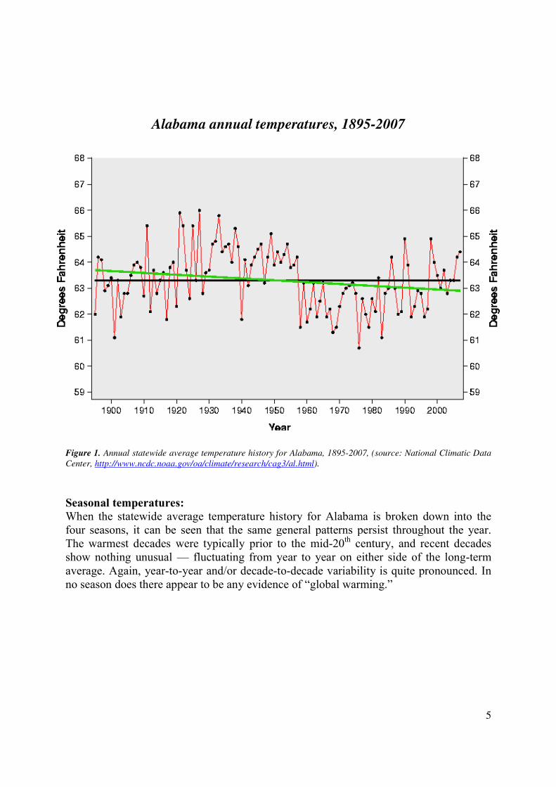
Alabama annual temperatures, 1895-2007

Figure 1. Annual statewide average temperature history for Alabama, 1895-2007, (source: National Climatic DataCenter, http://www.ncdc.noaa.gov/oa/climate/research/cag3/al.html).

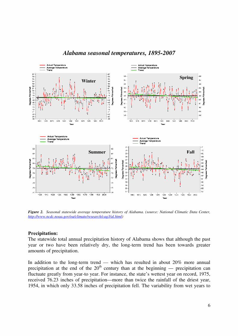
Seasonal temperatures:When the statewide average temperature history for Alabama is broken down into thefour seasons, it can be seen that the same general patterns persist throughout the year.The warmest decades were typically prior to the mid-20th century, and recent decadesshow nothing unusual — fluctuating from year to year on either side of the long-termaverage. Again, year-to-year and/or decade-to-decade variability is quite pronounced. Inno season does there appear to be any evidence of “global warming.”

6

Alabama seasonal temperatures, 1895-2007

Figure 2. Seasonal statewide average temperature history of Alabama. (source: National Climatic Data Center,http://www.ncdc.noaa.gov/oa/climate/research/cag3/al.html)

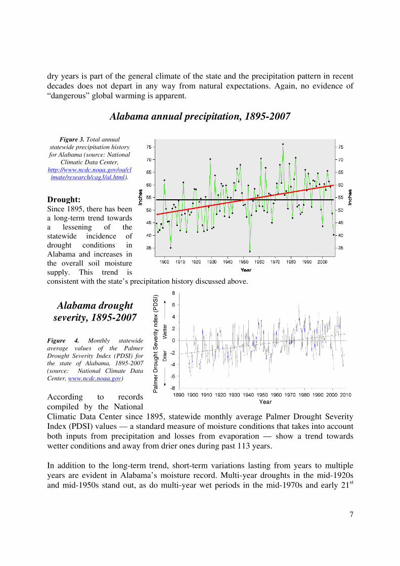
Precipitation:The statewide total annual precipitation history of Alabama shows that although the pastyear or two have been relatively dry, the long-term trend has been towards greateramounts of precipitation.

In addition to the long-term trend — which has resulted in about 20% more annualprecipitation at the end of the 20th century than at the beginning — precipitation canfluctuate greatly from year-to year. For instance, the state’s wettest year on record, 1975,received 76.23 inches of precipitation—more than twice the rainfall of the driest year,1954, in which only 33.58 inches of precipitation fell. The variability from wet years to

WinterSpring

Summer Fall

7

dry years is part of the general climate of the state and the precipitation pattern in recentdecades does not depart in any way from natural expectations. Again, no evidence of“dangerous” global warming is apparent.

Alabama annual precipitation, 1895-2007

Figure 3. Total annualstatewide precipitation historyfor Alabama (source: National

Climatic Data Center,http://www.ncdc.noaa.gov/oa/climate/research/cag3/al.html).

Drought:Since 1895, there has beena long-term trend towardsa lessening of thestatewide incidence ofdrought conditions inAlabama and increases inthe overall soil moisturesupply. This trend isconsistent with the state’s precipitation history discussed above.

Alabama droughtseverity, 1895-2007

Figure 4. Monthly statewideaverage values of the PalmerDrought Severity Index (PDSI) forthe state of Alabama, 1895-2007(source: National Climate DataCenter, www.ncdc.noaa.gov)

According to recordscompiled by the NationalClimatic Data Center since 1895, statewide monthly average Palmer Drought SeverityIndex (PDSI) values — a standard measure of moisture conditions that takes into accountboth inputs from precipitation and losses from evaporation — show a trend towardswetter conditions and away from drier ones during past 113 years.

In addition to the long-term trend, short-term variations lasting from years to multipleyears are evident in Alabama’s moisture record. Multi-year droughts in the mid-1920sand mid-1950s stand out, as do multi-year wet periods in the mid-1970s and early 21st

8

century. Dry conditions which characterize the past year or two are a natural part of theregion’s climate and not an unusual occurrence that could be related to “global warming.”

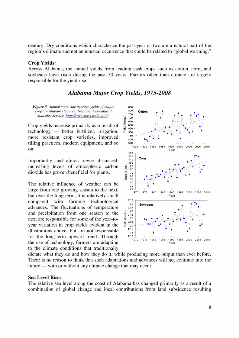
Crop Yields:Across Alabama, the annual yields from leading cash crops such as cotton, corn, andsoybeans have risen during the past 30 years. Factors other than climate are largelyresponsible for the yield rise.

Alabama Major Crop Yields, 1975-2008

Figure 5. Annual statewide average yields of majorcrops in Alabama (source: National Agricultural

Statistics Service, http://www.nass.usda.gov/).

Crop yields increase primarily as a result oftechnology — better fertilizer, irrigation,more resistant crop varieties, improvedtilling practices, modern equipment, and soon.

Importantly and almost never discussed,increasing levels of atmospheric carbondioxide has proven beneficial for plants.

The relative influence of weather can belarge from one growing season to the next,but over the long-term, it is relatively smallcompared with farming technologicaladvances. The fluctuations of temperatureand precipitation from one season to thenext are responsible for some of the year-to-year variation in crop yields evident in theillustrations above; but are not responsiblefor the long-term upward trend. Throughthe use of technology, farmers are adaptingto the climate conditions that traditionallydictate what they do and how they do it, while producing more output than ever before.There is no reason to think that such adaptations and advances will not continue into thefuture — with or without any climate change that may occur.

Sea Level Rise:The relative sea level along the coast of Alabama has changed primarily as a result of acombination of global change and local contributions from land subsidence resulting

9

from on-going geologic processes. While land subsidence dominates the relative rate ofsea level rise further west along the Gulf Coast, the shores of Alabama have fairly securegeologic bedding such that the rates of land subsidence are relatively small. The total rateof sea level rise along the Alabama Gulf Coast has been about 3mm/yr (or about 1 footper 100 years) over the past half-century or so. As the rising population of Alabama’scoastal communities attests, the residents of Alabama have adapted to this on-going rateof sea level rise.

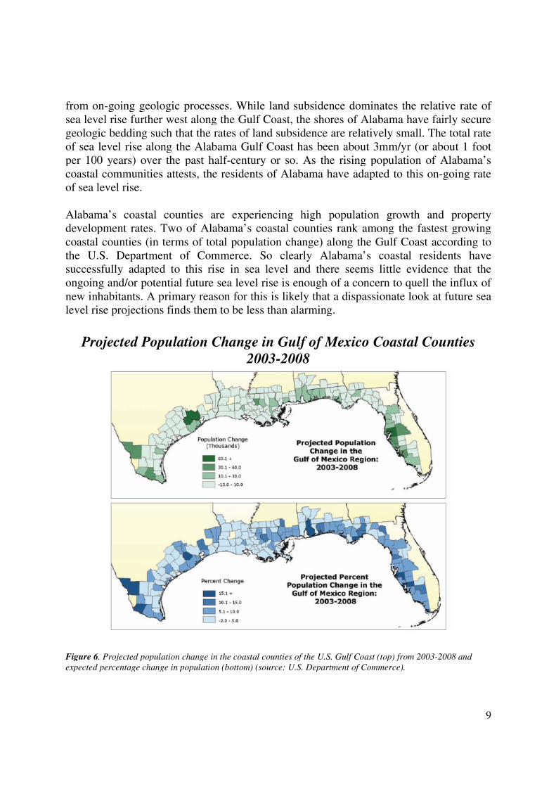
Alabama’s coastal counties are experiencing high population growth and propertydevelopment rates. Two of Alabama’s coastal counties rank among the fastest growingcoastal counties (in terms of total population change) along the Gulf Coast according tothe U.S. Department of Commerce. So clearly Alabama’s coastal residents havesuccessfully adapted to this rise in sea level and there seems little evidence that theongoing and/or potential future sea level rise is enough of a concern to quell the influx ofnew inhabitants. A primary reason for this is likely that a dispassionate look at future sealevel rise projections finds them to be less than alarming.

Projected Population Change in Gulf of Mexico Coastal Counties2003-2008

Figure 6. Projected population change in the coastal counties of the U.S. Gulf Coast (top) from 2003-2008 andexpected percentage change in population (bottom) (source: U.S. Department of Commerce).

10

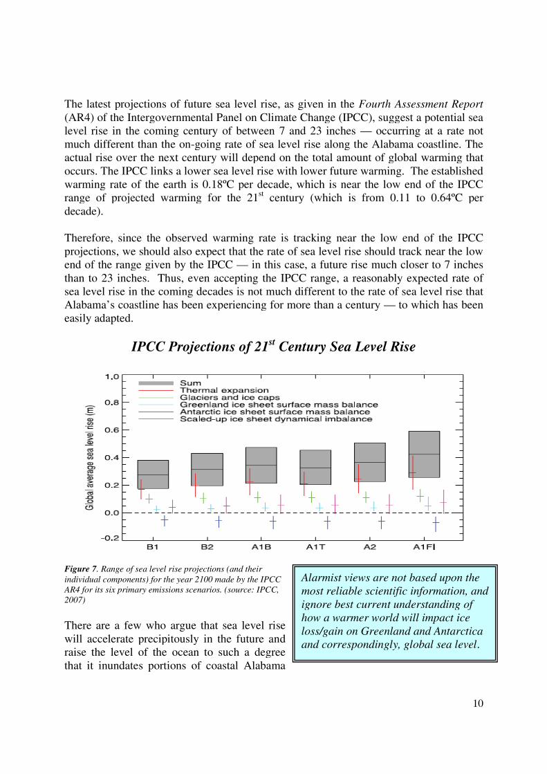
The latest projections of future sea level rise, as given in the Fourth Assessment Report(AR4) of the Intergovernmental Panel on Climate Change (IPCC), suggest a potential sealevel rise in the coming century of between 7 and 23 inches — occurring at a rate notmuch different than the on-going rate of sea level rise along the Alabama coastline. Theactual rise over the next century will depend on the total amount of global warming thatoccurs. The IPCC links a lower sea level rise with lower future warming. The establishedwarming rate of the earth is 0.18ºC per decade, which is near the low end of the IPCCrange of projected warming for the 21st century (which is from 0.11 to 0.64ºC perdecade).

Therefore, since the observed warming rate is tracking near the low end of the IPCCprojections, we should also expect that the rate of sea level rise should track near the lowend of the range given by the IPCC — in this case, a future rise much closer to 7 inchesthan to 23 inches. Thus, even accepting the IPCC range, a reasonably expected rate ofsea level rise in the coming decades is not much different to the rate of sea level rise thatAlabama’s coastline has been experiencing for more than a century — to which has beeneasily adapted.

IPCC Projections of 21st Century Sea Level Rise

Figure 7. Range of sea level rise projections (and theirindividual components) for the year 2100 made by the IPCCAR4 for its six primary emissions scenarios. (source: IPCC,2007)

There are a few who argue that sea level risewill accelerate precipitously in the future andraise the level of the ocean to such a degreethat it inundates portions of coastal Alabama

Alarmist views are not based upon themost reliable scientific information, andignore best current understanding ofhow a warmer world will impact iceloss/gain on Greenland and Antarcticaand correspondingly, global sea level.

11

and other low-lying areas around the world and they clamor that the IPCC was far tooconservative in its projections.

However, these rather alarmist views are not based upon the most reliable scientificinformation, and ignore best current understanding of how a warmer world will impactice loss/gain on Greenland and Antarctica and correspondingly, global sea level. It is afact, that all of the extant models of the future of Antarctica indicate that a warmerclimate leads to more snowfall, the majority of which remains for hundreds to thousandsof years because it is so cold. This acts to slow the rate of global sea level rise becausethe water remains trapped in ice and snow. New data suggest that rapid rates of ice lossfrom Greenland in the future are not likely (Joughin et al., 2008; van de Wal et al. 2008).Scenarios of disastrous rises in sea level are predicated upon Antarctica and Greenlandlosing massive amounts of snow and ice in a very short period of time — an occurrencewith zero likelihood.

An author of the IPCC AR4 chapter dealing with sea level rise projections, Dr. RichardAlley, recently testified before the House Committee on Science and Technologyconcerning the state of scientific knowledge of accelerating sea level rise and pressure toexaggerate what it known about it. Dr. Alley told the Committee:

This document [the IPCC AR4] works very, very hard to be an assessment of whatis known scientifically and what is well-founded in the refereed literature andwhen we come up to that cliff and look over and say we don’t have a foundationright now, we have to tell you that, and on this particular issue, the trend ofacceleration of this flow with warming we don’t have a good assessedscientific foundation right now. [emphasis added]

Thus, the IPCC projections of future sea level rise, which average only about 15 inchesfor the next 100 years, stand as the best projections that can be made based upon ourcurrent level of scientific understanding. These projections are far less severe that thealarming projections of many feet of sea level rise that have been made by a fewindividuals whose views lie outside of the scientific consensus.

Extreme events - Hurricanes:

While Alabama’s rather short coastlinemakes direct hurricane landfalls ratherinfrequent, Alabama’s residents know alltoo well that whether a major hurricanemakes a direct strike (2004’s HurricaneIvan) or comes ashore nearby (2005’sHurricane Katrina), the impacts can bedevastating. Consequently, the state’s

While Alabama’s rather short coastlinemakes direct hurricane landfalls ratherinfrequent, Alabama’s residents knowall too well that whether a majorhurricane makes a direct strike (2004’sHurricane Ivan) or comes ashorenearby (2005’s Hurricane Katrina), theimpacts can be devastating.

12

interest in the potential influence of global warming on the past, present, and futuretrends in hurricane frequency and/or intensity is reasonable. Fortunately, our bestscientific understanding is that global warming will have a minor, if at all detectable,impact on Atlantic and Gulf hurricanes.

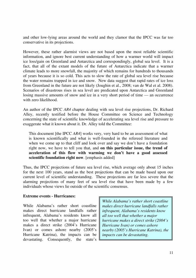
Since 1995 there has been a short-termincrease in the frequency of tropical stormsand hurricanes in the Atlantic basin. Whilesome scientists have attempted to link thisincrease to anthropogenic global warming,others have pointed out that Atlantichurricanes exhibit long-term cycles, and that this latest upswing is simply a return toconditions that characterized earlier decades in the 20th century.

Natural cycles dominate the observed record of Atlantic tropical cyclones, which dateback to the 18th and 19th centuries (e.g., Chylek and Lesins, 2008). Multi-decadaloscillations are obvious in the long-term record of hurricane activity in the Atlantic basin— hurricane activity was quiet in the 1910s and 1920s, elevated in the 1950s and 1960s,quiet in the 1970s and 1980s, and has picked up again since 1995.

Atlantic Hurricane Activity, 1930-2007

Figure 8. Annual number of tropical cyclones and major hurricanes observed in the Atlantic basin, 1930-2007.Bars depict number of named systems (light gay) and major ( category 3 or greater) hurricanes (dark gray) (source:National Hurricane Center).

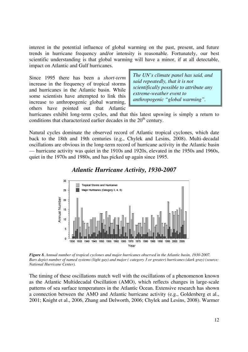
The timing of these oscillations match well with the oscillations of a phenomenon knownas the Atlantic Multidecadal Oscillation (AMO), which reflects changes in large-scalepatterns of sea surface temperatures in the Atlantic Ocean. Extensive research has showna connection between the AMO and Atlantic hurricane activity (e.g., Goldenberg et al.,2001; Knight et al., 2006, Zhang and Delworth, 2006; Chylek and Lesins, 2008). Warmer

The UN’s climate panel has said, andsaid repeatedly, that it is notscientifically possible to attribute anyextreme-weather event toanthropogenic “global warming”.

13

cycles of the AMO — such as currently — are associated with enhanced tropical cycloneactivity in the Atlantic Ocean and Gulf of Mexico, while the cold phase of the AMO isassociated with lessened storm activity. Analyzing patterns in paleoclimate datasetscoupled with model simulations, the AMO can be simulated back for more than 1,400years (Knight et al., 2005). This is strong evidence that the AMO is part of the earth’snatural climate variations and cycles, and not a consequence of recent “global warming.”

Further, not only is there evidence that the AMO has been operating for at least manycenturies prior to any possible human influence on the climate, but there is also growingevidence that there have been active and inactive periods in the Atlantic hurricanefrequency and strength extending many centuries into the past. For instance, research byMiller et al. (2006) using oxygen isotope information stored in tree-rings in thesoutheastern United States, finds distinct periods of activity/inactivity in a record datingback 220 years. In research that examined sediment records deposited from beachoverwash in a lagoon in Puerto Rico, scientists Donnelly and Woodruff (2007) haveidentified patterns of Atlantic tropical cyclone activity extending back 5,000 years.

Atlantic Multidecadal Oscillation (AMO)

Figure 9. The observed historical timeseries of the Atlantic Multidecadal Oscillation (AMO) (from Goldenberg etal., 2001).

14

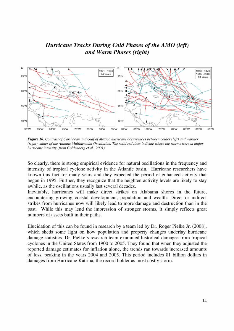
Hurricane Tracks During Cold Phases of the AMO (left)and Warm Phases (right)

Figure 10. Contrast of Caribbean and Gulf of Mexico hurricane occurrences between colder (left) and warmer(right) values of the Atlantic Multidecadal Oscillation. The solid red lines indicate where the storms were at majorhurricane intensity (from Goldenberg et al., 2001).

So clearly, there is strong empirical evidence for natural oscillations in the frequency andintensity of tropical cyclone activity in the Atlantic basin. Hurricane researchers haveknown this fact for many years and they expected the period of enhanced activity thatbegan in 1995. Further, they recognize that the heighten activity levels are likely to stayawhile, as the oscillations usually last several decades.Inevitably, hurricanes will make direct strikes on Alabama shores in the future,encountering growing coastal development, population and wealth. Direct or indirectstrikes from hurricanes now will likely lead to more damage and destruction than in thepast. While this may lend the impression of stronger storms, it simply reflects greatnumbers of assets built in their paths.

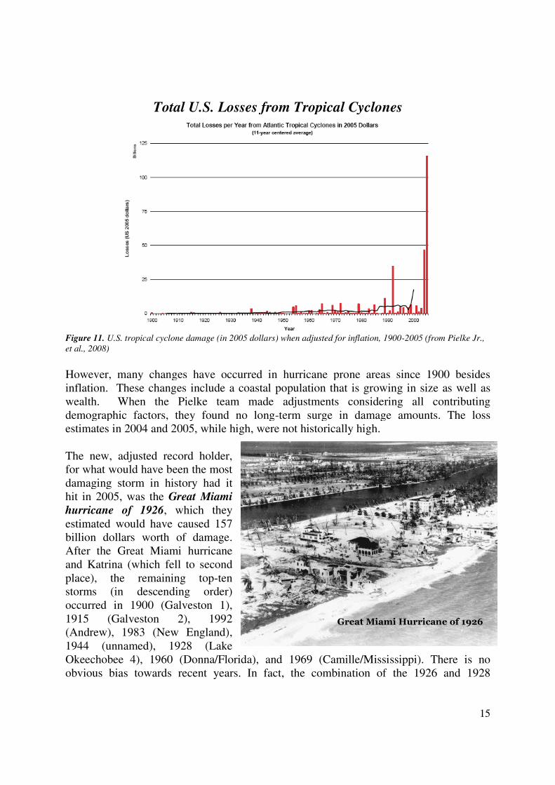
Elucidation of this can be found in research by a team led by Dr. Roger Pielke Jr. (2008),which sheds some light on how population and property changes underlay hurricanedamage statistics. Dr. Pielke’s research team examined historical damages from tropicalcyclones in the United States from 1900 to 2005. They found that when they adjusted thereported damage estimates for inflation alone, the trends ran towards increased amountsof loss, peaking in the years 2004 and 2005. This period includes 81 billion dollars indamages from Hurricane Katrina, the record holder as most costly storm.

15

Total U.S. Losses from Tropical Cyclones

Figure 11. U.S. tropical cyclone damage (in 2005 dollars) when adjusted for inflation, 1900-2005 (from Pielke Jr.,et al., 2008)

However, many changes have occurred in hurricane prone areas since 1900 besidesinflation. These changes include a coastal population that is growing in size as well aswealth. When the Pielke team made adjustments considering all contributingdemographic factors, they found no long-term surge in damage amounts. The lossestimates in 2004 and 2005, while high, were not historically high.

The new, adjusted record holder,for what would have been the mostdamaging storm in history had ithit in 2005, was the Great Miamihurricane of 1926, which theyestimated would have caused 157billion dollars worth of damage.After the Great Miami hurricaneand Katrina (which fell to secondplace), the remaining top-tenstorms (in descending order)occurred in 1900 (Galveston 1),1915 (Galveston 2), 1992(Andrew), 1983 (New England),1944 (unnamed), 1928 (LakeOkeechobee 4), 1960 (Donna/Florida), and 1969 (Camille/Mississippi). There is noobvious bias towards recent years. In fact, the combination of the 1926 and 1928

Great Miami Hurricane of 1926

16

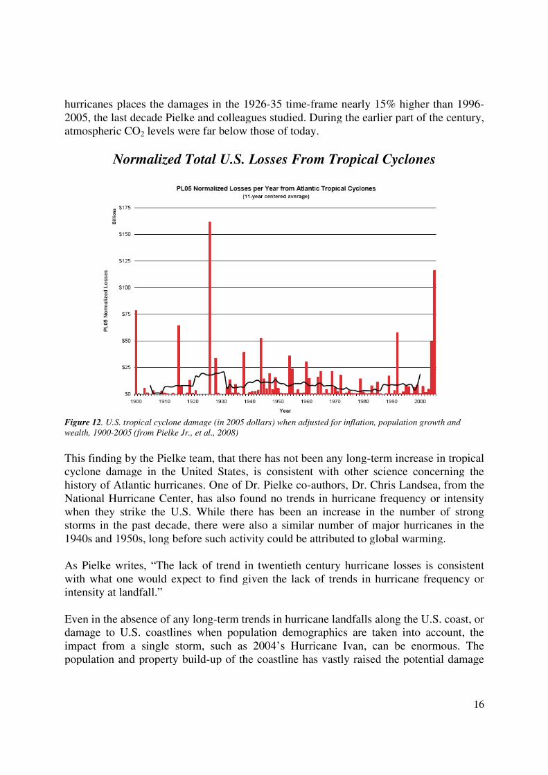
hurricanes places the damages in the 1926-35 time-frame nearly 15% higher than 1996-2005, the last decade Pielke and colleagues studied. During the earlier part of the century,atmospheric CO2 levels were far below those of today.

Normalized Total U.S. Losses From Tropical Cyclones

Figure 12. U.S. tropical cyclone damage (in 2005 dollars) when adjusted for inflation, population growth andwealth, 1900-2005 (from Pielke Jr., et al., 2008)

This finding by the Pielke team, that there has not been any long-term increase in tropicalcyclone damage in the United States, is consistent with other science concerning thehistory of Atlantic hurricanes. One of Dr. Pielke co-authors, Dr. Chris Landsea, from theNational Hurricane Center, has also found no trends in hurricane frequency or intensitywhen they strike the U.S. While there has been an increase in the number of strongstorms in the past decade, there were also a similar number of major hurricanes in the1940s and 1950s, long before such activity could be attributed to global warming.

As Pielke writes, “The lack of trend in twentieth century hurricane losses is consistentwith what one would expect to find given the lack of trends in hurricane frequency orintensity at landfall.”

Even in the absence of any long-term trends in hurricane landfalls along the U.S. coast, ordamage to U.S. coastlines when population demographics are taken into account, theimpact from a single storm, such as 2004’s Hurricane Ivan, can be enormous. Thepopulation and property build-up of the coastline has vastly raised the potential damage

17

that a storm can inflict. Recently, a collection of some of the world’s leading hurricaneresearchers issued the following statement that reflects the current thinking on hurricanesand their potential impact (http://wind.mit.edu/~emanuel/Hurricane_threat.htm):

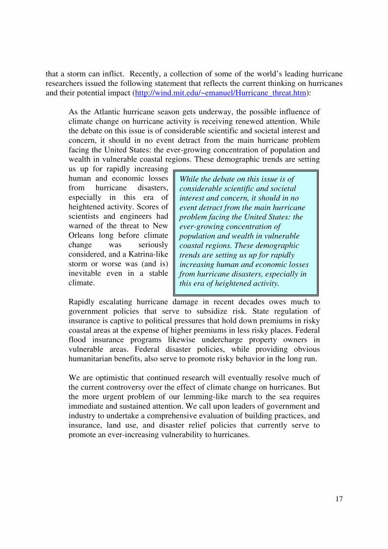
As the Atlantic hurricane season gets underway, the possible influence ofclimate change on hurricane activity is receiving renewed attention. Whilethe debate on this issue is of considerable scientific and societal interest andconcern, it should in no event detract from the main hurricane problemfacing the United States: the ever-growing concentration of population andwealth in vulnerable coastal regions. These demographic trends are settingus up for rapidly increasinghuman and economic lossesfrom hurricane disasters,especially in this era ofheightened activity. Scores ofscientists and engineers hadwarned of the threat to NewOrleans long before climatechange was seriouslyconsidered, and a Katrina-likestorm or worse was (and is)inevitable even in a stableclimate.

Rapidly escalating hurricane damage in recent decades owes much togovernment policies that serve to subsidize risk. State regulation ofinsurance is captive to political pressures that hold down premiums in riskycoastal areas at the expense of higher premiums in less risky places. Federalflood insurance programs likewise undercharge property owners invulnerable areas. Federal disaster policies, while providing obvioushumanitarian benefits, also serve to promote risky behavior in the long run.

We are optimistic that continued research will eventually resolve much ofthe current controversy over the effect of climate change on hurricanes. Butthe more urgent problem of our lemming-like march to the sea requiresimmediate and sustained attention. We call upon leaders of government andindustry to undertake a comprehensive evaluation of building practices, andinsurance, land use, and disaster relief policies that currently serve topromote an ever-increasing vulnerability to hurricanes.

While the debate on this issue is ofconsiderable scientific and societalinterest and concern, it should in noevent detract from the main hurricaneproblem facing the United States: theever-growing concentration ofpopulation and wealth in vulnerablecoastal regions. These demographictrends are setting us up for rapidlyincreasing human and economic lossesfrom hurricane disasters, especially inthis era of heightened activity.

18

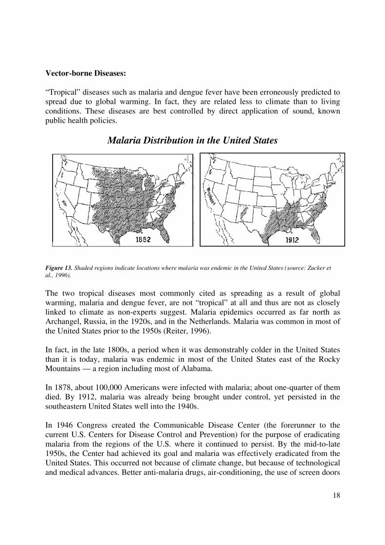
Vector-borne Diseases:

“Tropical” diseases such as malaria and dengue fever have been erroneously predicted tospread due to global warming. In fact, they are related less to climate than to livingconditions. These diseases are best controlled by direct application of sound, knownpublic health policies.

Malaria Distribution in the United States

Figure 13. Shaded regions indicate locations where malaria was endemic in the United States (source: Zucker etal., 1996).

The two tropical diseases most commonly cited as spreading as a result of globalwarming, malaria and dengue fever, are not “tropical” at all and thus are not as closelylinked to climate as non-experts suggest. Malaria epidemics occurred as far north asArchangel, Russia, in the 1920s, and in the Netherlands. Malaria was common in most ofthe United States prior to the 1950s (Reiter, 1996).

In fact, in the late 1800s, a period when it was demonstrably colder in the United Statesthan it is today, malaria was endemic in most of the United States east of the RockyMountains — a region including most of Alabama.

In 1878, about 100,000 Americans were infected with malaria; about one-quarter of themdied. By 1912, malaria was already being brought under control, yet persisted in thesoutheastern United States well into the 1940s.

In 1946 Congress created the Communicable Disease Center (the forerunner to thecurrent U.S. Centers for Disease Control and Prevention) for the purpose of eradicatingmalaria from the regions of the U.S. where it continued to persist. By the mid-to-late1950s, the Center had achieved its goal and malaria was effectively eradicated from theUnited States. This occurred not because of climate change, but because of technologicaland medical advances. Better anti-malaria drugs, air-conditioning, the use of screen doors

19

and windows, and the elimination of urban overpopulation brought about by thedevelopment of suburbs and automobile commuting were largely responsible for thedecline in malaria (Reiter, 1996; Reiter, 2001). Today, the mosquitoes that spread malariaare still widely present in the Unites States, but the transmission cycle has been disruptedand the pathogen leading to the disease is absent. Climate change is not involved.

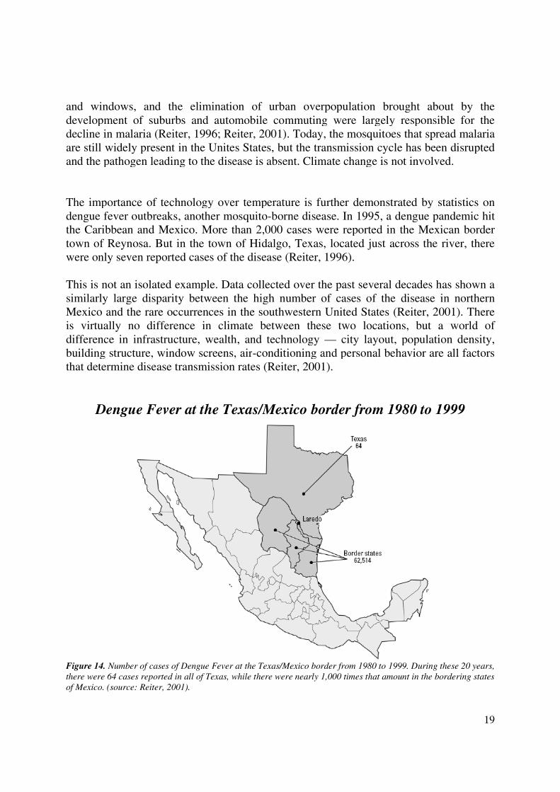
The importance of technology over temperature is further demonstrated by statistics ondengue fever outbreaks, another mosquito-borne disease. In 1995, a dengue pandemic hitthe Caribbean and Mexico. More than 2,000 cases were reported in the Mexican bordertown of Reynosa. But in the town of Hidalgo, Texas, located just across the river, therewere only seven reported cases of the disease (Reiter, 1996).

This is not an isolated example. Data collected over the past several decades has shown asimilarly large disparity between the high number of cases of the disease in northernMexico and the rare occurrences in the southwestern United States (Reiter, 2001). Thereis virtually no difference in climate between these two locations, but a world ofdifference in infrastructure, wealth, and technology — city layout, population density,building structure, window screens, air-conditioning and personal behavior are all factorsthat determine disease transmission rates (Reiter, 2001).

Dengue Fever at the Texas/Mexico border from 1980 to 1999

Figure 14. Number of cases of Dengue Fever at the Texas/Mexico border from 1980 to 1999. During these 20 years,there were 64 cases reported in all of Texas, while there were nearly 1,000 times that amount in the bordering statesof Mexico. (source: Reiter, 2001).

20

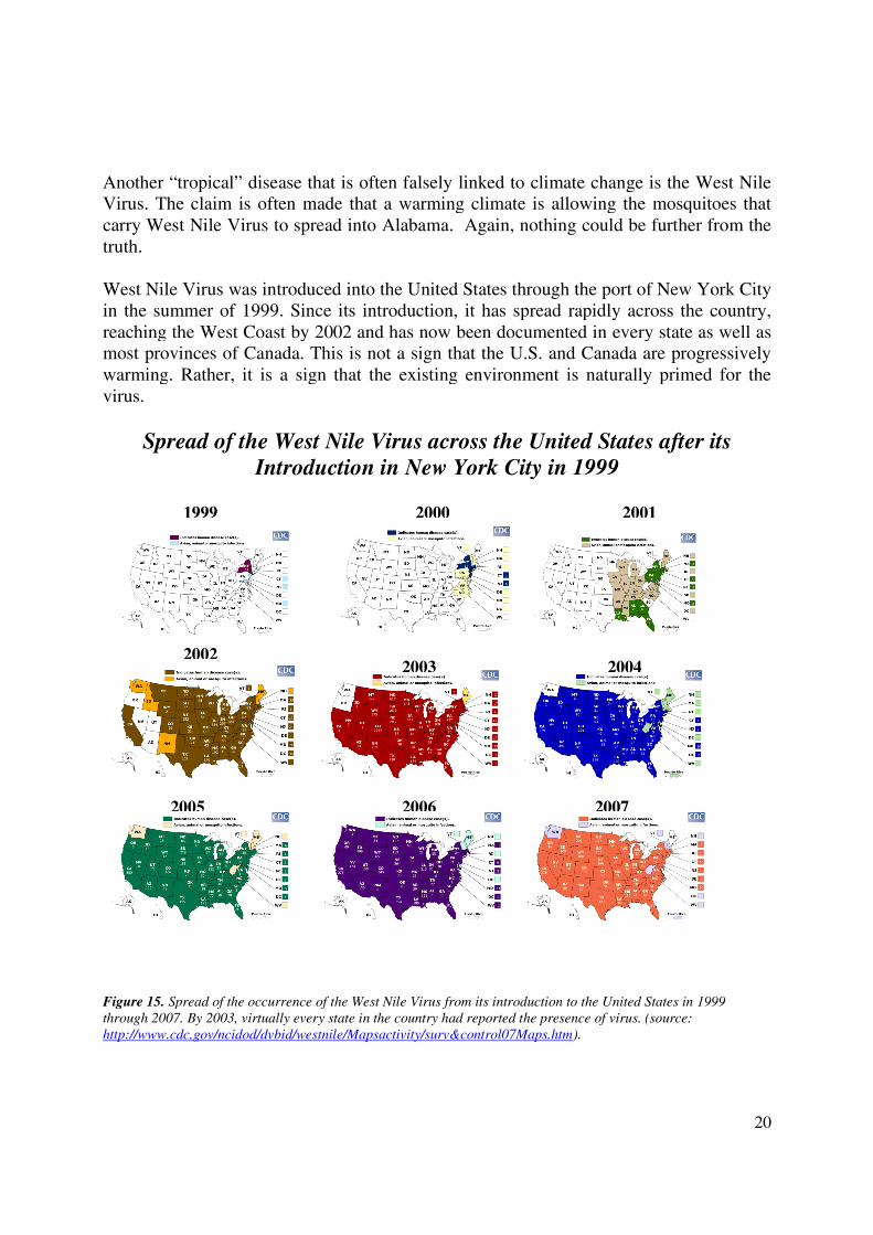
Another “tropical” disease that is often falsely linked to climate change is the West NileVirus. The claim is often made that a warming climate is allowing the mosquitoes thatcarry West Nile Virus to spread into Alabama. Again, nothing could be further from thetruth.

West Nile Virus was introduced into the United States through the port of New York Cityin the summer of 1999. Since its introduction, it has spread rapidly across the country,reaching the West Coast by 2002 and has now been documented in every state as well asmost provinces of Canada. This is not a sign that the U.S. and Canada are progressivelywarming. Rather, it is a sign that the existing environment is naturally primed for thevirus.

Spread of the West Nile Virus across the United States after itsIntroduction in New York City in 1999

Figure 15. Spread of the occurrence of the West Nile Virus from its introduction to the United States in 1999through 2007. By 2003, virtually every state in the country had reported the presence of virus. (source:http://www.cdc.gov/ncidod/dvbid/westnile/Mapsactivity/surv&control07Maps.htm).

2000 20011999

20022003 2004

2005 2006 2007

21

The vector for West Nile is mosquitoes; wherever there is a suitable host mosquitopopulation, an outpost for West Nile virus can be established. And it is not just onemosquito species that is involved. Instead, the disease has been isolated in over 40mosquito species found throughout the United States. So the simplistic argument thatclimate change is allowing a West Nile carrying mosquito species to move into Alabamais simply wrong. The already-resident mosquito populations of Alabama are appropriatehosts for the West Nile virus — as is true in every other state.

Clearly, as is evident from the establishment of West Nile virus in every state in thecontiguous U.S., climate has little, or nothing, to do with its spread. The annual averagetemperature from the southern part of the United States to the northern part spans a rangeof more than 40ºF, so clearly the virus exists in vastly different climates. In fact, WestNile virus was introduced in New York City — hardly the warmest portion of thecountry—and has spread westward and southward into both warmer and colder andwetter and drier climates. This didn’t happen because climate changes facilitated itsspread, but instead because the virus was introduced into a place that was ripe for itsexistence — basically any location with a resident mosquito population: basicallyanywhere in the U.S.

West Nile virus now exists in Alabama because the extant climate/ecology of Alabama isone in which the virus can thrive. The reason that it was not found in Alabama in the pastwas simply because it had not been introduced. Temperature trends in Alabama hadabsolutely nothing to do with it (as fig. 1 shows, the temperature trend over the centurywas downward). Besides, by following the virus’ progression from 1999 through 2007,one clearly sees that the virus spread from the cooler region of NYC southward andwestward, it did not invade slowly from the warmer south, as one would have expected ifwarmer temperatures really was the driver.

Thus, since the disease spreads in a wide range of both temperature and climatic regimes,one could raise or lower the average annual temperature in Alabama by many degrees orvastly change the precipitation regime and not make a bit of difference in the aggressionof the West Nile Virus. Science-challenged claims to the contrary are not only ignorantbut also dangerous, serving to distract from real epidemiological diagnosis which allowshealth officials critical information for protecting the citizens of Alabama.

Put another way, demonstrably false claims by climate activities about disease causesputs at risk the health and lives of Alabama citizens, particularly that of children and theelderly.

22

Impacts of climate-mitigation measures in the state ofAlabama

Globally, in 2004, humankind emitted 27,186 million metric tons of carbon dioxide(mmtCO2), of which emissions from Alabama accounted for 140.3 mmtCO2, or a mere0.52% (EIA, 2007; EIA, 2008). The proportion of manmade CO2 emissions fromAlabama will decrease over the 21st century as the rapid demand for power in developingcountries such as China and India rapidly outpaces the growth of Alabama’s CO2

emissions (EIA, 2007).

During the past 5 years, global emissions of CO2 from human activity have increased atan average rate of 3.5%/yr (EIA, 2007), meaning that the annual global increase ofanthropogenic global CO2 emissions is nearly 7 times greater than Alabama’s totalemissions. Put differently, even a complete cessation of all CO2 emissions in Alabamawould be completely subsumed by global emissions growth in under two month’s time!

In fact, China alone adds about four Alabama’s-worth of new emissions to its emissionstotal each and every year. Thus, a complete cessation of all CO2 emissions in Alabamawould be completely subsumed by Chinese emissions growth in about 84 days!

Clearly, given the magnitude of the global and Chinese emissions growth, regulationsprescribing a total cessation of Alabama’s CO2 emissions would have absolutely zeroeffect on global climate. Thus, any schedule of incremental reductions would be evenmore vanishingly insignificant and futile.

Wigley (1998) examined the climate impact of adherence to the emissions controlsagreed under the Kyoto Protocol by participating nations, and found that, if all developedcountries meet their commitments in 2010 and maintain them through 2100, with a mid-range sensitivity of surface temperature to changes in CO2, the amount of warming“saved” by the Kyoto Protocol would be 0.07°C by 2050 and 0.15°C by 2100. The globalsea level rise “saved” would be 2.6 cm, or one inch.

Even a complete cessation of CO2 emissions in Alabama is only a tiny fraction of theworldwide reductions assumed in Dr. Wigley’s global analysis, so its impact on futuretrends in global temperature and sea level will be only a minuscule fraction of thenegligible effects calculated by Dr. Wigley.

To demonstrate the futility of emissions regulations in Alabama, we apply Dr. Wigley’sresults to the state, assuming that the ratio of U.S. CO2 emissions to those of thedeveloped countries which have agreed to limits under the Kyoto Protocol remainsconstant at 39% (25% of global emissions) throughout the 21st century. We also assumethat developing countries such as China and India continue to emit at an increasing rate.

23

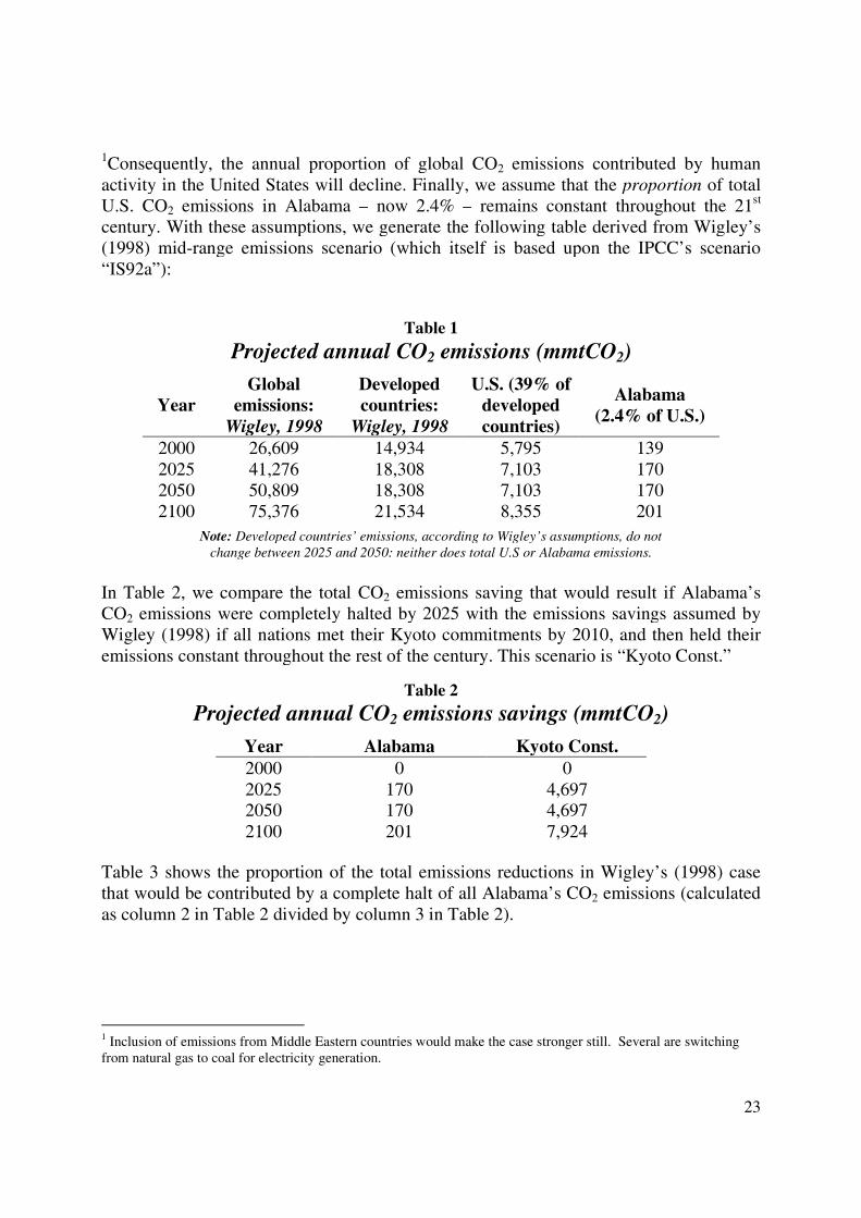
1Consequently, the annual proportion of global CO2 emissions contributed by humanactivity in the United States will decline. Finally, we assume that the proportion of totalU.S. CO2 emissions in Alabama – now 2.4% – remains constant throughout the 21st

century. With these assumptions, we generate the following table derived from Wigley’s(1998) mid-range emissions scenario (which itself is based upon the IPCC’s scenario“IS92a”):

Table 1

Projected annual CO2 emissions (mmtCO2)

YearGlobal

emissions:Wigley, 1998

Developedcountries:

Wigley, 1998

U.S. (39% ofdevelopedcountries)

Alabama(2.4% of U.S.)

2000 26,609 14,934 5,795 1392025 41,276 18,308 7,103 1702050 50,809 18,308 7,103 1702100 75,376 21,534 8,355 201

Note: Developed countries’ emissions, according to Wigley’s assumptions, do notchange between 2025 and 2050: neither does total U.S or Alabama emissions.

In Table 2, we compare the total CO2 emissions saving that would result if Alabama’sCO2 emissions were completely halted by 2025 with the emissions savings assumed byWigley (1998) if all nations met their Kyoto commitments by 2010, and then held theiremissions constant throughout the rest of the century. This scenario is “Kyoto Const.”

Table 2

Projected annual CO2 emissions savings (mmtCO2)

Year Alabama Kyoto Const.2000 0 02025 170 4,6972050 170 4,6972100 201 7,924

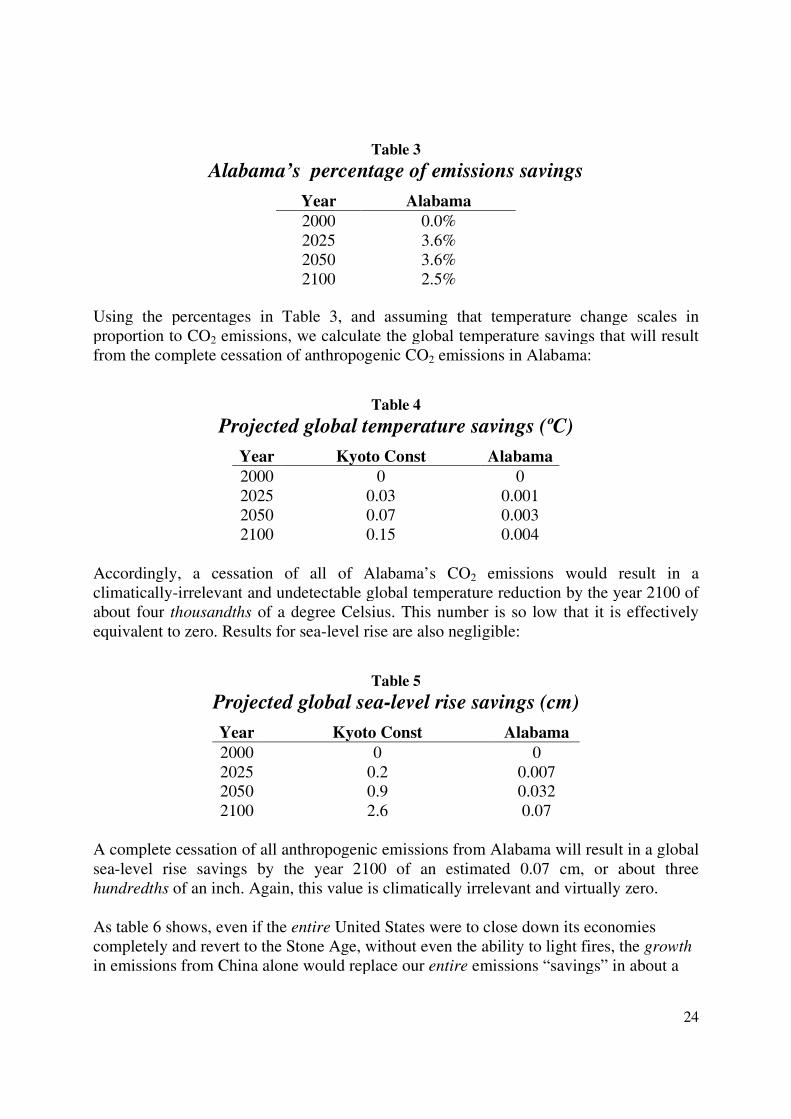
Table 3 shows the proportion of the total emissions reductions in Wigley’s (1998) casethat would be contributed by a complete halt of all Alabama’s CO2 emissions (calculatedas column 2 in Table 2 divided by column 3 in Table 2).

1 Inclusion of emissions from Middle Eastern countries would make the case stronger still. Several are switchingfrom natural gas to coal for electricity generation.

24

Table 3

Alabama’s percentage of emissions savings

Year Alabama2000 0.0%2025 3.6%2050 3.6%2100 2.5%

Using the percentages in Table 3, and assuming that temperature change scales inproportion to CO2 emissions, we calculate the global temperature savings that will resultfrom the complete cessation of anthropogenic CO2 emissions in Alabama:

Table 4

Projected global temperature savings (ºC)

Year Kyoto Const Alabama2000 0 02025 0.03 0.0012050 0.07 0.0032100 0.15 0.004

Accordingly, a cessation of all of Alabama’s CO2 emissions would result in aclimatically-irrelevant and undetectable global temperature reduction by the year 2100 ofabout four thousandths of a degree Celsius. This number is so low that it is effectivelyequivalent to zero. Results for sea-level rise are also negligible:

Table 5

Projected global sea-level rise savings (cm)

Year Kyoto Const Alabama2000 0 02025 0.2 0.0072050 0.9 0.0322100 2.6 0.07

A complete cessation of all anthropogenic emissions from Alabama will result in a globalsea-level rise savings by the year 2100 of an estimated 0.07 cm, or about threehundredths of an inch. Again, this value is climatically irrelevant and virtually zero.

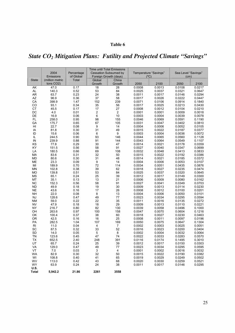
As table 6 shows, even if the entire United States were to close down its economiescompletely and revert to the Stone Age, without even the ability to light fires, the growthin emissions from China alone would replace our entire emissions “savings” in about a

25

Table 6

State CO2 Mitigation Plans: Futility and Projected Climate “Savings”

Time until Total EmissionsCessation Subsumed byForeign Growth (days)

Temperature “Savings”(ºC)

Sea Level “Savings”(cm)

State

2004Emissions

(million metrictons CO2)

Percentageof Global

Total GlobalGrowth

ChinaGrowth 2050 2100 2050 2100

AK 47.0 0.17 18 28 0.0008 0.0013 0.0108 0.0217AL 140.3 0.52 53 84 0.0025 0.0037 0.0321 0.0647AR 63.7 0.23 24 38 0.0011 0.0017 0.0146 0.0294AZ 96.9 0.36 37 58 0.0017 0.0026 0.0222 0.0447CA 398.9 1.47 152 239 0.0071 0.0106 0.0914 0.1840CO 93.1 0.34 35 56 0.0017 0.0025 0.0213 0.0430CT 45.5 0.17 17 27 0.0008 0.0012 0.0104 0.0210DC 4.0 0.01 2 2 0.0001 0.0001 0.0009 0.0018DE 16.9 0.06 6 10 0.0003 0.0004 0.0039 0.0078FL 258.0 0.95 98 155 0.0046 0.0069 0.0591 0.1190GA 175.7 0.65 67 105 0.0031 0.0047 0.0402 0.0810HI 22.7 0.08 9 14 0.0004 0.0006 0.0052 0.0105IA 81.8 0.30 31 49 0.0015 0.0022 0.0187 0.0377ID 15.6 0.06 6 9 0.0003 0.0004 0.0036 0.0072IL 244.5 0.90 93 146 0.0044 0.0065 0.0560 0.1128IN 239.9 0.88 91 144 0.0043 0.0064 0.0549 0.1107KS 77.8 0.29 30 47 0.0014 0.0021 0.0178 0.0359KY 151.5 0.56 58 91 0.0027 0.0040 0.0347 0.0699LA 180.5 0.66 69 108 0.0032 0.0048 0.0413 0.0833MA 83.6 0.31 32 50 0.0015 0.0022 0.0192 0.0386MD 80.6 0.30 31 48 0.0014 0.0021 0.0185 0.0372ME 23.3 0.09 9 14 0.0004 0.0006 0.0053 0.0107MI 189.9 0.70 72 114 0.0034 0.0051 0.0435 0.0876MN 102.8 0.38 39 62 0.0018 0.0027 0.0235 0.0474MO 139.8 0.51 53 84 0.0025 0.0037 0.0320 0.0645MS 65.1 0.24 25 39 0.0012 0.0017 0.0149 0.0300MT 35.1 0.13 13 21 0.0006 0.0009 0.0080 0.0162NC 152.3 0.56 58 91 0.0027 0.0041 0.0349 0.0703ND 49.9 0.18 19 30 0.0009 0.0013 0.0114 0.0230NE 43.6 0.16 17 26 0.0008 0.0012 0.0100 0.0201NH 22.0 0.08 8 13 0.0004 0.0006 0.0050 0.0101NJ 128.6 0.47 49 77 0.0023 0.0034 0.0295 0.0594NM 59.0 0.22 22 35 0.0011 0.0016 0.0135 0.0272NV 47.9 0.18 18 29 0.0009 0.0013 0.0110 0.0221NY 216.7 0.80 82 130 0.0039 0.0058 0.0496 0.1000OH 263.6 0.97 100 158 0.0047 0.0070 0.0604 0.1216OK 100.4 0.37 38 60 0.0018 0.0027 0.0230 0.0463OR 42.5 0.16 16 25 0.0008 0.0011 0.0097 0.0196PA 282.5 1.04 107 169 0.0050 0.0075 0.0647 0.1304RI 11.0 0.04 4 7 0.0002 0.0003 0.0025 0.0051SC 87.5 0.32 33 52 0.0016 0.0023 0.0200 0.0404SD 14.0 0.05 5 8 0.0002 0.0004 0.0032 0.0064TN 123.6 0.45 47 74 0.0022 0.0033 0.0283 0.0570TX 652.5 2.40 248 391 0.0116 0.0174 0.1495 0.3010UT 65.7 0.24 25 39 0.0012 0.0017 0.0150 0.0303VA 129.0 0.47 49 77 0.0023 0.0034 0.0295 0.0595VT 7.0 0.03 3 4 0.0001 0.0002 0.0016 0.0032WA 82.9 0.30 32 50 0.0015 0.0022 0.0190 0.0382WI 108.8 0.40 41 65 0.0019 0.0029 0.0249 0.0502WV 113.0 0.42 43 68 0.0020 0.0030 0.0259 0.0521WY 63.9 0.24 24 38 0.0011 0.0017 0.0146 0.0295U.S.Total 5,942.2 21.86 2261 3558

26

decade. In this context, any cuts in emissions from Alabama would be extravagantlypointless. Alabama’s carbon dioxide emissions, it their sum total, effectively do notimpact world climate in any way whatsoever.

Pres-Elect Obama’s Cap and Trade Proposal

President-elect Obama has promised to “bankrupt” the coal industry with the most

draconian cap and trade scheme in the world.

Under his announced greenhouse gas emissions reduction plan, he proposes to reduce

the U.S.’s annual greenhouse house gas emissions total such that the U.S. total

emissions in the year 2020 are the same as what the U.S. total emissions were in the

year 1990. Even further, he vows to reduce total greenhouse gas emissions from the

U.S. to 80% below what they were in 1990 by the year 2050.

The numbers look something like this (all numbers are in million metric tons CO2):

Year U.S. CO2 Emissions

1990 5013

2007 5984

Obama’s Proposed Target

Year CO2 Emissions Savings from 2007 level Savings/year

2020 5013 971 75

2050 1003 4981 116

Now, let’s compare the total emissions savings (under the Obama plan) to annual

growth in CO2 emissions from countries besides the United States.

27

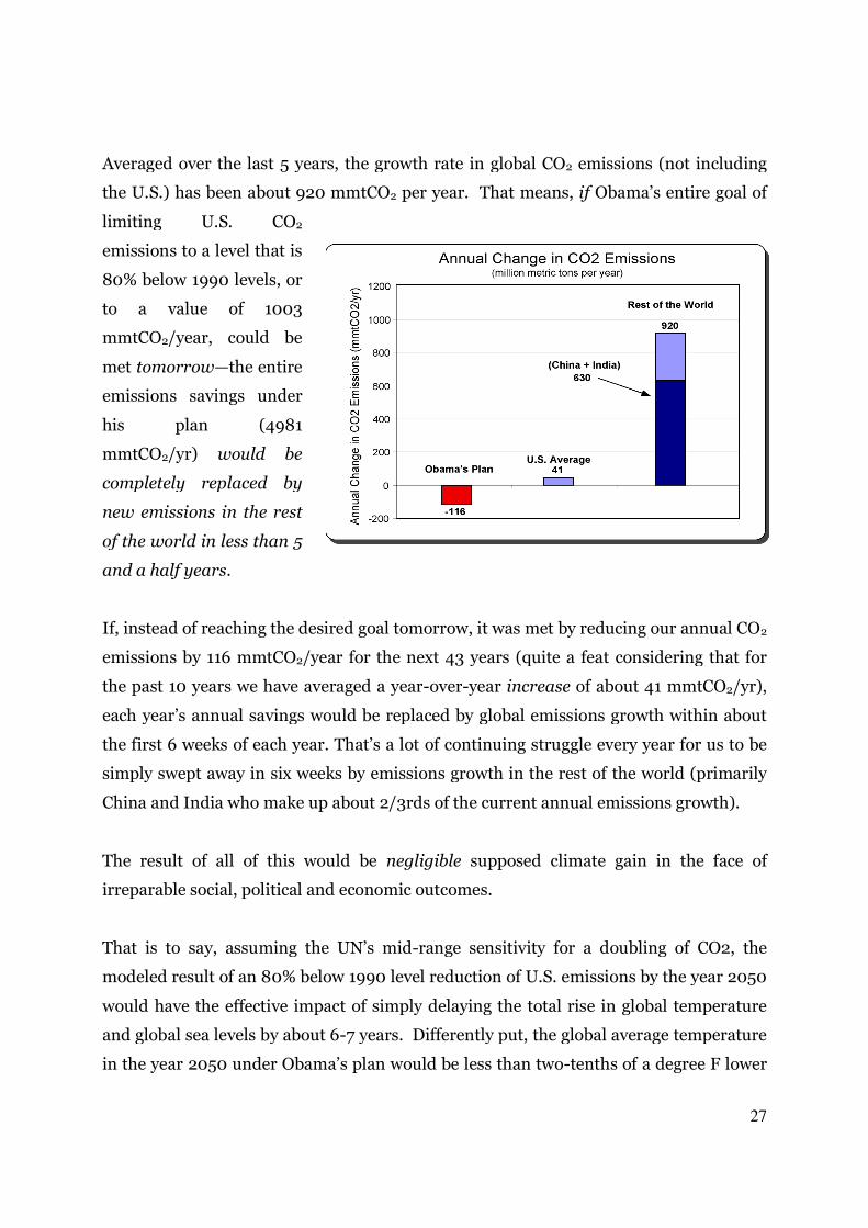
Averaged over the last 5 years, the growth rate in global CO2 emissions (not including

the U.S.) has been about 920 mmtCO2 per year. That means, if Obama’s entire goal of

limiting U.S. CO2

emissions to a level that is

80% below 1990 levels, or

to a value of 1003

mmtCO2/year, could be

met tomorrow—the entire

emissions savings under

his plan (4981

mmtCO2/yr) would be

completely replaced by

new emissions in the rest

of the world in less than 5

and a half years.

If, instead of reaching the desired goal tomorrow, it was met by reducing our annual CO2

emissions by 116 mmtCO2/year for the next 43 years (quite a feat considering that for

the past 10 years we have averaged a year-over-year increase of about 41 mmtCO2/yr),

each year’s annual savings would be replaced by global emissions growth within about

the first 6 weeks of each year. That’s a lot of continuing struggle every year for us to be

simply swept away in six weeks by emissions growth in the rest of the world (primarily

China and India who make up about 2/3rds of the current annual emissions growth).

The result of all of this would be negligible supposed climate gain in the face of

irreparable social, political and economic outcomes.

That is to say, assuming the UN’s mid-range sensitivity for a doubling of CO2, the

modeled result of an 80% below 1990 level reduction of U.S. emissions by the year 2050

would have the effective impact of simply delaying the total rise in global temperature

and global sea levels by about 6-7 years. Differently put, the global average temperature

in the year 2050 under Obama’s plan would be less than two-tenths of a degree F lower

28

than it otherwise would have been in the year 2050. The global sea level would be about

one-half an inch lower than where it otherwise would have been.

These impacts on the climate [even if scientifically believable] are, for all intents and

purposes scientifically and physically meaningless.

Impact of the European Union Actions – and other Nations

Oftentimes, the actions of the European Union aimed towards reducing carbon dioxide

emissions are held up as an example of how to combat climate change through decisive

government action. But as with the U.S., the EU is actually quite ineffective when it

comes to actually making a difference on global climate by regulating CO2.

It is no secret that the EU talks the talk about climate change, but it doesn't walk the

walk. Most EU countries will fail to meet their Kyoto emissions-reduction targets. While

the much-reviled US administration succeeded in quietly cutting total US carbon

emissions in recent years, the EU's carbon emissions have increased. Also, the EU's first

attempt at carbon trading ended in characteristic farce when all member-states except

the UK awarded themselves emissions rights that comfortably exceeded previous

emissions. Result: the "price" of carbon emissions per ton of CO2 fell below 50 cents,

rendering the entire scheme useless. No climatic benefit ensued, and none will ensue

from the EU's current scheme, which is nothing more than a purposeless extra cost to

already hard-pressed businesses, many of which are finding it simpler to move out of

the EU altogether.

In fact, even if the entirety of the EU-27 nations were to completely and forever cease all

CO2 emissions from this day forward, it would have an insignificant impact on the

course of the world’s future climate (Table 2). In 50 years, the global temperature

“savings” produced by an immediate cessation of all EU-27 CO2 emissions is estimated

to be less than one-tenth of a degree Celsius, and increasing to just a bit more than a

tenth of a degree by centuries end. The impacts of future sea level would be equally

miniscule.

29

Needless to say, the efforts to simply reduce CO2 emissions from individual countries

within the EU-27 produce even less of in impact—effectively no climate moderation…no

lessening of the global temperature rise, no slowing of global sea level rise, nothing.

Worse, all of their efforts will be quickly subsumed by new CO2 emissions resulting

from the rapid development and accompanying growth in emissions from the rest of the

world, primarily China and India. In fact, a complete cessation of all EU-27 CO2

emissions would be subsumed by new emissions from the rest of the world in under 4 ½

years. For individual EU countries, the timing is even more disheartening. For example,

growth in emissions from China would replace the entirety of Austria’s annual emissions

in just 47 days, those from Denmark in 31, Spain’s in less than 8 months, and those from

the U.K. in just under a year. Monumental efforts gone within a relative blink of an eye.

Ditto for Australia, New Zealand and Japan.

This is a scenario that — just as in the U.S. — is best described as one which produces no

climate gain for incredible economic pain.

SPPI: Additional Readings in Climate Science

Environmental Effects of Increased Atmospheric Carbon Dioxidehttp://scienceandpublicpolicy.org/other/increasedco2effects.html

35 Inconvenient Truths: The errors in Al Gore’s moviehttp://scienceandpublicpolicy.org/monckton/goreerrors.html

Hockey Stick? What Hockey Stick?http://scienceandpublicpolicy.org/monckton/what_hockey_stick.html

An unscientific “Science Brief” by the Pew Center on “The Causes of Global Climate Change”http://scienceandpublicpolicy.org/originals/pew_center_science_brief.html

Letter to Senator McCainhttp://scienceandpublicpolicy.org/reprint/letter_to_mccain.html

Sherwood and Craig Idso examine James Hansen’s Senate testimony.http://scienceandpublicpolicy.org/other/sherwood_and_craig_idso_examine_james_hansen_s_recent_senate_test

imony.html

30

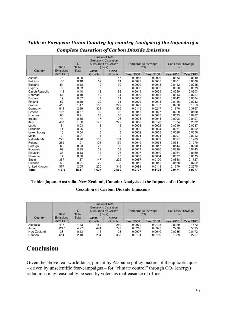
Table 2: European Union Country-by-country Analysis of the Impacts of a

Complete Cessation of Carbon Dioxide Emissions

Time until TotalEmissions CessationSubsumed by Growth

(days)Temperature “Savings”

(ºC)Sea Level “Savings”

(cm)Country

2005Emissions(mmt CO2)

%GlobalTotal Global

GrowthChina

Growth Year 2050 Year 2100 Year 2050 Year 2100Austria 78 0.28 30 47 0.0013 0.0020 0.0173 0.0349Belgium 136 0.48 52 81 0.0023 0.0035 0.0301 0.0606Bulgaria 51 0.18 19 30 0.0009 0.0013 0.0112 0.0225Cyprus 9 0.03 3 5 0.0002 0.0002 0.0020 0.0039Czech Republic 113 0.40 43 68 0.0019 0.0029 0.0250 0.0503Denmark 51 0.18 19 31 0.0009 0.0013 0.0113 0.0227Estonia 19 0.07 7 11 0.0003 0.0005 0.0042 0.0084Finland 52 0.19 20 31 0.0009 0.0013 0.0116 0.0233France 415 1.47 158 249 0.0072 0.0107 0.0920 0.1853Germany 844 2.99 321 505 0.0145 0.0217 0.1870 0.3767Greece 103 0.37 39 62 0.0018 0.0027 0.0229 0.0460Hungary 60 0.21 23 36 0.0010 0.0015 0.0133 0.0267Ireland 44 0.16 17 26 0.0008 0.0011 0.0098 0.0197Italy 467 1.66 178 279 0.0080 0.0120 0.1034 0.2082Latvia 8 0.03 3 5 0.0001 0.0002 0.0019 0.0037Lithuania 14 0.05 5 8 0.0002 0.0004 0.0031 0.0062Luxembourg 13 0.04 5 8 0.0002 0.0003 0.0028 0.0056Malta 3 0.01 1 2 0.0001 0.0001 0.0007 0.0013Netherlands 270 0.96 103 161 0.0046 0.0069 0.0597 0.1203Poland 285 1.01 108 170 0.0049 0.0073 0.0631 0.1270Portugal 65 0.23 25 39 0.0011 0.0017 0.0144 0.0290Romania 99 0.35 38 59 0.0017 0.0026 0.0220 0.0443Slovakia 38 0.13 14 23 0.0007 0.0010 0.0084 0.0169Slovenia 17 0.06 6 10 0.0003 0.0004 0.0037 0.0075Spain 387 1.37 147 232 0.0067 0.0100 0.0858 0.1727Sweden 59 0.21 22 35 0.0010 0.0015 0.0130 0.0262United Kingdom 577 2.05 220 346 0.0099 0.0149 0.1279 0.2575Total 4,276 15.17 1,627 2,560 0.0737 0.1101 0.9471 1.9077

Table: Japan, Australia, New Zealand, Canada: Analysis of the Impacts of a Complete

Cessation of Carbon Dioxide Emissions

Time until TotalEmissions CessationSubsumed by Growth

(days)Temperature “Savings”

(ºC)Sea Level “Savings”

(cm)Country

2006Emissions(mmt CO2)

%GlobalTotal Global

GrowthChina

Growth Year 2050 Year 2100 Year 2050 Year 2100Australia 417 1.43 159 250 0.0072 0.0108 0.0929 0.1872Japan 1247 4.27 474 747 0.0216 0.0323 0.2778 0.5595New Zealand 38 0.13 15 23 0.0007 0.0010 0.0085 0.0172Canada 614 2.10 234 368 0.0101 0.0159 0.1369 0.2757

Conclusion

Given the above real-world facts, pursuit by Alabama policy makers of the quixotic quest– driven by unscientific fear-campaigns – for “climate control” through CO2 (energy)reductions may reasonably be seen by voters as malfeasance of office.

31

Costs of Federal Legislation

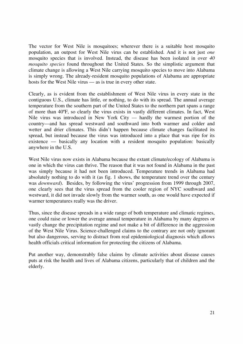
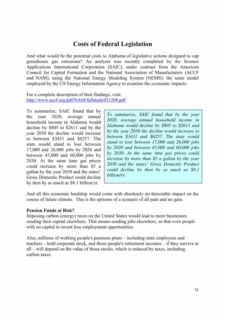
And what would be the potential costs to Alabama of legislative actions designed to capgreenhouse gas emissions? An analysis was recently completed by the ScienceApplications International Corporation (SAIC), under contract from the AmericanCouncil for Capital Formation and the National Association of Manufacturers (ACCFand NAM), using the National Energy Modeling System (NEMS); the same modelemployed by the US Energy Information Agency to examine the economic impacts.

For a complete description of their findings, visit:http://www.accf.org/pdf/NAM/fullstudy031208.pdf

To summarize, SAIC found that bythe year 2020, average annualhousehold income in Alabama woulddecline by $805 to $2611 and by theyear 2030 the decline would increaseto between $3431 and $6257. Thestate would stand to lose between17,000 and 26,000 jobs by 2020 andbetween 45,000 and 60,000 jobs by2030. At the same time gas pricescould increase by more than $5 agallon by the year 2030 and the states’Gross Domestic Product could declineby then by as much as $8.1 billion/yr.

And all this economic hardship would come with absolutely no detectable impact on thecourse of future climate. This is the epitome of a scenario of all pain and no gain.

Pension Funds at Risk?Imposing carbon (energy) taxes on the United States would lead to more businessessending their capital elsewhere. That means sending jobs elsewhere, so that even peoplewith no capital to invest lose employment opportunities.

Also, millions of working people's pensions plans – including state employees andteachers – hold corporate stock, and those people's retirement incomes – if they survive atall – will depend on the value of those stocks, which is reduced by taxes, includingcarbon taxes.

To summarize, SAIC found that by the year2020, average annual household income inAlabama would decline by $805 to $2611 andby the year 2030 the decline would increase tobetween $3431 and $6257. The state wouldstand to lose between 17,000 and 26,000 jobsby 2020 and between 45,000 and 60,000 jobsby 2030. At the same time gas prices couldincrease by more than $5 a gallon by the year2030 and the states’ Gross Domestic Productcould decline by then by as much as $8.1billion/yr.

32

Part of the severe results of futile CO2 reduction plans could be crippling of Alabama’smajor public sector pension funds. The state has two major pension funds for itsworkers.

Alabama Employees Retirement System has$9.2 billion in actuarial assets and $11.4billion actuarial liabilities.

The Alabama Teachers Retirement Systemhas $19.8 in actuarial assets and $23.9 billionin actuarial liabilities.

The systems rely on the following assumptions: 8.0 percent annual investment return and4.50 percent annual inflation. As of 12/31/06, about 43 percent of the Public Employeefund portfolio was in equities.

Both funds currently pass the "80 percent" test-- assets should be at least 80% of liabilities.Alabama’s ERS is funded at 81.1 percent whilethe Teachers fund is as 82.8%. But thesefigures are as of 9-30-07 when the marketswere substantially higher than before thecurrent -- October 2008 -- financial crisis.

Current Alabama workers and pensionersshould be very, very concerned about their jobs

and retirement funds if state and/or federal regulatory attacks through CO2 mitigationplans reduce GDP, kill jobs, reduce tax revenues and further erode equity markets.

Part of the severe results of futileCO2 reduction plans could becrippling of Alabama’s major publicsector pension funds.

Current Alabama workers andpensioners should be very, veryconcerned about their jobs andretirement funds if state and/orfederal regulatory attacks throughCO2 mitigation plans reduce GDP,kill jobs, reduce tax revenues andfurther erode equity markets.

33

Figure 16. The projected economic impacts in Alabama of federal legislation to limit greenhouse gasemissions green. (Source: Science Applications International Corporation, 2008,http://www.instituteforenergyresearch.org/cost-of-climate-change-policies/)

Alabama Scientists Reject UN’s Global Warming Claims2

At least 485 Alabama scientists agree in principle with our analysis, they havingpetitioned the Federal government that the UN’s human-caused global warminghypothesis is “without scientific validity and that government action on the basis of thishypothesis would unnecessarily and counterproductively damage both human prosperityand the natural environment of the Earth.”

They are joined by over 31,072 Americans with university degrees in science – including9,021 PhDs.

The petition and entire list of US signers can be found here:http://www.petitionproject.org/index.html

Names of the Alabama scientists who signed the petition can be viewed here:http://petitionproject.org/gwdatabase/Signers_BY_State.html

2 Questions about this survey should be addressed to the petition organizers.

34

Appendix: Recent global temperatures: As the global temperature graphbelow shows, all four of the world’s major global surface temperature datasets (NASAGISS; RSS; UAH; and Hadley/University of East Anglia) show a decline in temperaturesthat have now persisted for seven years. The fall in temperatures between January 2007and January 2008 was the greatest January-January fall since records began in 1880.

All four of the world’s major surface-temperature datasets show seven yearsof global cooling. The straight lines are the regression lines showing the trend

over past seven years. It is decisively downward.

Lower-troposphere global surface temperature anomalies, 1979-2008 (UAH satellite data).

The year 2008 will turn out to have been no warmer than 1980 – 28 years ago. This is nota short-run change: the cooling trend set in as far back as late 2001, seven full years ago,and there has been no net warming since 1995 on any measure.

35

References

Chylek, P., and G. Lesins (2008), Multi-decadal variability of Atlantic hurricane activity: 1851-2007, J.Geophys. Res., doi:10.1029/2008JD010036, in press.

Donnelly, J.P., and J.D. Woodruff. 2007. Intense hurricane activity over the past 5,000 years controlledby El Niño and the West African monsoon. Nature, 447, 465-468.

Energy Information Administration, 2007. International Energy Annual, 2005 (and updates) U.S.Department of Energy, Washington, D.C., http://www.eia.doe.gov/iea/contents.html

Energy Information Administration, 2008. State-by-state carbon dioxide emissions available on-line athttp://www.eia.doe.gov/oiaf/1605/ggrpt/excel/tbl_statetotal.

Goldenberg, S., et al., 2001.The recent increase in Atlantic hurricane activity: Causes and implications.Science, 293, 474-479.

Intergovernmental Panel on Climate Change, 2007. Summary for Policymakers,(http://www.ipcc.ch/SPM2feb07.pdf)

Joughin, I., et al., 2008. Seasonal speedup along the western flank of the Greenland Ice Sheet. Science,320, 781-783 (http://www.sciencemag.org/cgi/content/abstract/320/5877/781).

Knight, J.R., et al., 2005. A signal of natural thermohaline cycles in observed climate. GeophysicalResearch Letters, L20708, doi:10.1029/2005GL24233.

Knight, J.R., et al., 2006. Climate impacts of the Atlantic Multidecadal Oscillation. Geophysical ResearchLetters, L17706, doi:10.1029/2006GL026242.

Landsea, C. W., 2005. Hurricanes and global warming. Nature, 438, E11-13.

Miller, D.L., C.I. Mora, H.D. Grissino-Mayer, C.J. Mock, M.E. Uhle, and Z. Sharp, 2006. Tree-ring isotoperecords of tropical cyclone activity. Proceedings of the National Academy of Sciences, 103, 14,294-14,297.

National Climatic Data Center, U.S. National/State/Divisional Data,(www.ncdc.noaa.gov/oa/climate/climatedata.html)

Pielke Jr., R. A., et al., 2008. Normalized hurricane damages in the United States: 1900-2005. NaturalHazards Review, 9, 29-42.

Reiter, P., 1996. Global warming and mosquito-borne disease in the USA. The Lancet, 348, 662.

U. S. Department of Commerce, 2004 Population trends along the Coastal United States: 1980-2008,http://oceanservice.noaa.gov/programs/mb/supp_cstl_population.html

van de Wal, R. S. W., et al., 2008. Large and rapid melt-induced velocity changes in the ablation zone ofthe Greenland ice sheet. Science, 321, 111-113(http://www.sciencemag.org/cgi/content/abstract/321/5885/111)

Wigley, T.M.L., 1998. The Kyoto Protocol: CO2, CH4 and climate implications. Geophysical ResearchLetters, 25, 2285-2288.

36

Zhang, R., and T. Delworth, 2006. Impact of Atlantic Multidecadal Oscillation on India/Sahel rainfall andAtlantic hurricanes. Geophysical Research Letters, 33, L17712, doi:10.1029/2006GL026267.

Zucker, J.R., 1996. Changing patterns of autochthonous malaria transmission in the United States: Areview of recent outbreaks. Emerging Infectious Diseases, 2, 37-43.