Observer Design and Model Augmentation

for Bias Compensation Applied to an Engine

Erik Hockerdal ∗,∗∗, Erik Frisk ∗, and Lars Eriksson ∗

∗ Department of Electrical Engineering, Linkopings universitet,Sweden, {hockerdal,frisk,larer}@isy.liu.se

∗∗ Scania CV AB, Sodertalje, Sweden, erik.hockerdal@scania.com

Abstract: A systematic design method for reducing bias in observers is developed. The methodutilizes an observable default model of the system together with measurement data from the realsystem and estimates a model augmentation. The augmented model is then used to design anobserver which reduces the estimation bias compared to a default observer. A key result is thetheoretical analysis that characterizes the possible augmentations is also conducted. The methodis applied to a truck engine where the resulting augmented observer reduces the estimation biaswith 50 % in an ETC.

Keywords: bias compensation, EKF, non-linear, observer

1. INTRODUCTION

In all model based control or diagnosis systems, the perfor-mance of the system is directly dependent on the accuracyof the model. Further, modeling is time consuming and,even if much time is spent on physical modeling, therewill always be errors in the model. This is especially trueif there are constraints on the model complexity, as is thecase in most real time systems. Another scenario is thata model developed for some purpose, e.g. control, existsbut needs corrections before it can be used in for examplediagnosis.

In many applications, for example engine control andengine diagnosis, it is crucial to have unbiased estimates. Inmodel based diagnosis, the true system is often monitoredby comparing measured signals to estimated signals. Ifthe magnitude of the difference, the residual, is above acertain limit a decision that something is wrong is made.In engine control, the goal is to maximize torque outputwhile keeping the emissions below legislated levels and thefuel consumption as low as possible. For diesel engines thisis especially hard since the control system does not haveany feedback information from a λ- or NOx-sensor andhave to rely on estimated signals instead. In both cases,biased estimates impairs the performance.

The objective of this work is to develop a systematicmethod for reducing estimation bias in model based ob-servers without involving further modeling efforts.

The model utilizes an observable model of, and measure-ment data from a true system. The given model, referred toas the default model, and the measured inputs and outputsfrom the true system are used to estimate a suitablemodel augmentation. Then, the augmented model is usedto design an observer that is shown to give estimates withreduced bias compared to an observer based on the defaultmodel. A key result is a theoretical characterization of allpossible augmentations. Finally the method is evaluated

on a non-linear diesel engine model with experimental datafrom an engine test cell.

2. PROBLEM FORMULATION

Previous experience at Scania CV AB of state estimationbased on an existing state-space model of a truck enginereveals that the model captures dynamic behavior reason-ably well but suffers from stationary errors. Designing anobserver based on this model results in biased estimatesand how to reduce this problem in a systematic manner isthe topic of this paper.

The starting point is an existing model, referred to as thedefault model, that is provided in state-space form

x = f(x, u) (1a)

y = h(x), (1b)

where x is the state-vector, u the known control inputs,y the measurement vector, and f and h are non-linearfunctions.

The objective is to find a systematic way to design anobserver that gives an unbiased estimate of either thecomplete state x or a function of the state z = g(x). Thisshould be done even though the default model is subjectedto significant bias errors. A direct approach to compensatefor constant, or slowly varying, biases is to augment thedefault model with bias variables q as

x = f(x, u, q) (2a)

q = 0 (2b)

y = h(x, q) (2c)

and design the observer using this augmented model. If theaugmentation captures the true modeling errors and theaugmented system is observable, the observer estimatescan be made unbiased.

An obvious question is then how to introduce the biasvariable q in the model equations. One way is through

process knowledge but in this paper we propose an esti-mation procedure based on available measurement data.Besides the natural restriction, that the augmented model(2) is observable, it is also desirable to not introduce moreextra bias states than necessary. It is therefore desirable tofind a bias vector q with as low dimension as possible thatmanages to reduce the bias. Another reason for finding alow dimensional bias is that, since the model is a first-principles physical model, bias in multiple states may beexplained by one underlying bias affecting all these states.For example, bias in two pressures can originate from abias in the mass flow between the two volumes or anincorrect modeling of energy conservation can give rise tobias in several states connected to the energy.

In the model (1) there are two natural ways to introducebiases, in the dynamic equation (1a) or in the measurementequation (1b). In the truck engine application the sensors,intake and exhaust manifold pressures and turbine speed,are considered more reliable than the model and thebias augmentation is therefore introduced in the dynamicequations according to

x = f(x − Aqq, u) (3a)

q = 0 (3b)

y = h(x). (3c)

where a stationary point of the system is moved by Aqq.The matrix Aq is thus a description on how the underlyingbias variable q influences the stationary value of the statevariable x. The model (3) will be referred to as theaugmented model.

2.1 Problem outline

Based on the discussion above, the problem studied in thesections to follow can now be stated as: Given a defaultmodel (1) and available measurement data, find a loworder bias augmented model (3) and design an observerthat estimates x with reduced bias compared to using thedefault model. The observer should also be implementablein an Engine Control Unit (ECU).

To solve the problems, some issues need to be addressed.First, which matrices Aq are at all possible? Not allare possible since we require that the augmented systemshould be observable and a characterization of possibleaugmentations is derived in Section 3. Among these pos-sible bias augmentations, which should be used? Section 4describes three approaches for how to estimate a, for biascompensation, suitable low order Aq based on measure-ment data. Section 5 finally summarizes the procedure andSection 6 presents two examples of the proposed estimatordesign methodology applied to a Scania diesel engine usingsimulated and real measurement data respectively.

2.2 Discretization

As a first step, the nonlinear augmented model (3) is trans-formed to a linearized time discrete model. A reason forthe discretization is the demand on the implementation,which will be done in the ECU as a time discrete system.An Euler forward discretization with step size Ts seconds isused. The reasons for the linearization are, to simplify theobservability analysis and to get a model that fits into the

EKF frame-work used in the observer design. It is furtherassumed that conclusions on observability made locallycan be used to draw conclusions of the global observabilityproperties of the model. This gives the following model

[

xt+1

qt+1

]

=

[

I + TsA −TsAAq

0 I

] [

xt

qt

]

+

[

B0

]

ut (4a)

yt = [C 0]

[

xt

qt

]

, (4b)

where

A =∂f

∂x

∣

∣

∣

∣ x=x0

u=u0

, B =∂f

∂u

∣

∣

∣

∣ x=x0

u=u0

, and C =∂h

∂x

∣

∣

∣

∣ x=x0

u=u0

3. POSSIBLE AUGMENTATIONS

Augmenting a model with more states may affect theobservability of the model. Since the purpose of the aug-mented model is to use it for estimation, observability hasto be maintained also after the augmentation. To findwhich augmentations that are possible an observabilityinvestigation of the augmented model is performed. Theaim is to derive a necessary and sufficient condition onAq such that the augmented model is observable. The ob-servability criterion used is known as the Popov-Belevitch-Hautus(PBH)-test (Kailath, 1980).

Theorem 1. A pair (C,F ) is observable if and only if thematrix

O =

(

CF − λI

)

has full column rank for all λ ∈ C.

To proceed, two assumptions regarding the default modelare made. First, the default model is used for observerdesign and is therefore assumed to be observable. Second,A is assumed to be invertible, which is the case in theapplication example. Now, using Theorem 1 and the twoassumptions above, the main result of this section can beformulated as

Theorem 2. Assume that (C,A) in (4) is an observablepair and that A is non-singular, then the augmentedsystem is observable if and only if

ImAq ∩ Ker C = {0}

which is equivalent to CAq having full column rank.

Proof. The PBH-test applied to the augmented model (4)gives

Oaug =

C 0I + TsA − λI −TsAAq

0 I − λI

Since the default model is assumed to be observable, theupper left block in Oaug has full column rank for all λ andOaug can lose rank only for λ = 1. It is therefore sufficientto check the column rank of

(

C 0TsA −TsAAq

)

Which is equivalent to requiring that the only solution to

Cx = 0

TsA(x − Aqq) = 0

is x = 0, q = 0. Since A is non-singular this is equivalentto,

Cx = 0

x = Aqq

Hence the augmented system is observable if and only if

ImAq ∩ Ker C = {0}

or, equivalently, that the matrix CAq has full column rank.�

This means that the space spanned by the columns in Aq

can not lie in the null space of C for the augmented modelto be observable.

A closer look at the requirement that CAq has to havefull column rank convey some interesting results. Firstly,it is easily seen that the number of augmented states,nq = dim q, never can exceed the number of measurementsignals, ny = dim y, i.e. nq ≤ ny. Secondly, imagine a Cthat has one or several zero columns, then the productCAq will not contain any information from those rows inAq corresponding to the zero columns in C. That is, thoserows in Aq that correspond to zero columns in C will notcontribute to the observability.

Also note that the following results regarding observabilityare not dependent on the method chosen for discretization.As long as Ts is chosen small enough the results are validalso for, e.g. zero-order-hold (Kalman et al., 1963).

Example 1. Possible augmentations of a small system withinvertible A, and

C =

[

1 0 00 1 0

]

(1) An augmentation

Aq =

[

1 00 00 1

]

is not observable since CAq =

[

1 00 0

]

and does not have full column rank. The reason forthis is that the second column in Aq only has non-zero components in the row corresponding to the zerocolumn in C.

(2) However, if either of the two zeros in the secondcolumn of Aq is interchanged to, for example a one,the augmentation becomes observable.

Aq =

[

1 00 10 1

]

⇒ CAq =

[

1 00 1

]

⋄

4. AUGMENTATION ESTIMATION

The next question is how to find a suitable augmentation,that fulfills the requirements derived in Section 3, usingdata (y, u) from the real system. Three approaches for howto estimate a suitable augmentation have been developed.In the following, I + TsA is substituted for F to increasereadability.

4.1 Approach 1

The first approach utilizes the discretized linearizationdirectly,

xt+1 = Ftxt + (I − Ft)Aqqt + Btut

yt = Ctxt

Inverting the measurement equation and inserting theresulting x in the dynamic equation, gives

Aqqt = (I − Ft)−1(C†

t+1yt+1 − FtC†t yt − Btut),

where † denotes the pseudo inverse. To find a suitable aug-mentation, the Aqqt’s are collected in a matrix, RAqqt

=[Aqq1, . . . , AqqN ], which is analyzed by singular valuedecomposition (SVD). Here it is crucial that the SNR ishigh enough, otherwise the noise is a dominating part ofAqqt and an SVD would give a basis for the noise, not thebias. However, if the SNR is high enough the SVD gives abasis for the space in which the bias moves and Aq can bechosen to span that space.

An advantage with this approach over the other two is thatthere is no need for computing any intermediate observerfor estimating the augmentation. A disadvantage, besidesthat C has to have full column rank, is that, since no filteris involved, it is sensitive to measurement noise.

4.2 Approach 2

The second approach is based on an SVD of the residualsoriginating from an observer based on the default model.Here, the observer is an extended Kalman filter (EKF)(Kailath et al., 2000), where the noise covariance matricesQ and R are design parameters tuned by the user. Theestimation error becomes,

et+1 = xt+1 − xt+1|t+1

= Ftxt + (I − Ft)Aqq + Btut−

(Ftxt|t + Btut + Kt(yt+1 − CtFtxt|t − CtBtut))

= {yt+1 = CtFtxt + Ct(I − Ft)Aqq + CtBtut}

= (Ft − KtCtFt)et + (I − KtCt)(I − Ft)Aqq (7)

Equation (7) requires that the estimation error is knownwhich normally is not the case, hence the residuals,

rt = yt − yt|t = Ct(xt − xt|t) = Ctet, (8)

are used for estimating an augmentation. The fact thatresiduals from an observer is used instead of the mea-surements makes this approach less sensitive to low SNR,compared to Approach 1.

Here, solely stationary parts of the residuals are involvedwhen searching an appropriate augmentation, Aq. In theexample the stationary parts are separated out throughvisual inspection of the data at hand. It would be possibleto use also dynamical parts of the residuals and a dynami-cal inverse. The reason for not utilizing these is to preventdynamical estimation errors from affecting the estimationof the constant or slowly varying bias. This results in

rstat = Cstatestat

= Cstat(I − Fstat + KstatCstatFstat)−1×

(I − KstatCstat)(I − Fstat)Aqqstat

According to this Aq can be found by first finding thestationary residuals in a set of system operating points,collect these in the same way as in Approach 4.1, and per-form an SVD. The SVD returns a basis for the residuals,Vr, and Aq can be estimated as

Aq = (Cstat(I − Fstat + KstatCstatFstat)−1×

(I − KstatCstat)(I − Fstat))†Vr (9)

4.3 Approach 3

An alternative to Approach 2 for finding Aq is to augmentthe default model with as many extra states as possible.According to Theorem 2, CAq has to have full columnrank. This means that Aq can have a maximum of ny

columns, one non-zero element per column, and these non-zero elements have to correspond to non-zero columnsof C. Run the observer based on the augmented model,perform an SVD on the stationary parts of the augmentedstates, and assemble Aq.

An advantage with this approach is that no inversionsas those in (9) are needed. A disadvantage is that theorder of the observer may become quite large during theaugmentation estimation. In the worst case the order ofthe augmented model will be twice the order of the defaultmodel.

Example 2. Here the maximum possible augmentation isillustrated for a default model with

C =

[

1 0 00 1 0

]

Let × denote a non-zero element, then some possibleaugmentations are

A1q =

[

× 00 ×0 0

]

, and A2q =

[

0 ×× 00 0

]

since

CA1q =

[

× 00 ×

]

, and CA2q =

[

0 ×× 0

]

,

which have full column rank. While an augmentation

A3q =

[

× 00 00 ×

]

is not possible since CA3q =

[

× 00 0

]

does not have full column rank. ⋄

4.4 Remarks

The SVD returns a matrix, Vr, containing orthogonalvectors spanning the space in which the bias moves andthe corresponding singular values. The singular valuesconstitute the diagonal of a matrix, Sr and the i:thdiagonal element corresponds to the i:th column in Vr. Thesingular values in Sr are ordered in descending order whichmeans that the far left columns, corresponding to largesingular values, represent the most dominating directionsalong in the space in which the bias moves. Therefore thedimension of q can be found by comparing the singularvalues in Sr, and picking the most significant ones. Thenthe corresponding columns of Vr are used in the estimationof Aq.

Also note that, according to the discussion in the endof Section 3, the properties of C place restrictions onwhich Aq:s that are possible to find. The conclusionof that discussion is that rows in Aq corresponding tozero columns in C become zero in the estimation step.As a consequence, the observer based on an estimatedaugmentation may not be able to reduce the bias inthe estimates to acceptable levels. This problem can becircumvented in, for example one of the two following ways.The first is for an engineer to design an Aq not possible to

find through estimation, for example through knowledge ofthe underlying physics. The second is to add extra sensorsto the true system to acquire a full column rank C whichenables estimation of all rows in Aq.

The example below illustrates the remarks regarding theaffects the properties of C have on the augmentationestimation.

Example 3. Consider a true system with

F =

[

1 1 −1−1 0 11 1 −1

]

, and C =

[

1 0 00 1 0

]

and a true bias,

Aq =

[

111

]

Then the estimation of Aq, according to (9), will have thefollowing structure

Aq =

[

××0

]

That is, rows in Aq corresponding to zero columns in Ccan not be estimated. ⋄

5. METHOD

The procedure can be summarized in three steps.

Step 1 - Linearize and discretize the model if necessary.Normally, the default model is a non-linear time contin-uous model, (1), and has to be linearized and discretized.There are several ways to discretize a model, Eulerforward/backward, central difference etc, that have dif-ferent stability properties.

Step 2 - Find an appropriate augmentation, Aq, andcompile an augmented model (4). Here the designer hasa choice, either to estimate an augmentation from mea-sured data using one of the three approaches presentedin Section 4, or introduce an augmentation found insome other way. With good knowledge of the system,the designer might have some idea of what is causingthe bias in the estimates and can chose an appropriateAq.

Step 3 - Design an observer based on the augmentedmodel (3) and the Aq found in Step 2.

6. EXPERIMENTAL EVALUATION

To evaluate the approach two experiments are performedon a non-linear model of a truck engine.

In the first experiment the method is applied to syntheticdata created by introducing known biases in a non-linearmodel of a Diesel engine with three states. The states,x1, x2, and x3, represent intake and exhaust manifoldpressures, and turbine speed respectively, see Appendix A.In the second experiment, real data from the engine is usedtogether with the engine model to illustrate the gain in areal application.

In many real applications it is convenient to have a filterwhen estimating an augmentation to reduce the influenceof measurement noise, therefore approach 2 is chosen in

both these experiments. The observer based on the defaultmodel is referred to as the default observer while theobserver based on the augmented model is referred to asthe augmented observer.

6.1 Simulation study

The introduced bias is represented by

Aq =

[

1 −22 10 0

]

and two slowly varying biases q1 and q2. This Aq meansthat there are two independent biases affecting the pres-sures in the model which varies between approximately 0and 10 % of the state values. The default system has thelinear measurement equation where y1 = x1 and y2 = x3.However, according to the discussion in Section 4.4, anaugmentation as the one introduced in this example cannot be estimated without a direct connection between x2

and y. Therefore the measurement equation is extendedwith an extra sensor for x2. To make the simulation morerealistic, white system and measurement noise are addedin the creation of the synthetic data. Using the syntheticdata and the default model the augmentation estimationresults in

Sr ≈

[

136 0 00 30 00 0 0.01

]

, and Aq ≈

[

0.892 −0.4520.452 0.8920.017 0.006

]

where Sr indicates that there are two slowly varying biasespresent. Hence, Aq is estimated using the first two columnsof Vr and (9).

At a first look Aq does not appear similar to Aq. However,

the crucial fact is that the columns of Aq and Aq span,approximately, the same space. A closer look reveals thatthe elements in the bottom row is significantly smaller thanthe other elements, and that the factor between row oneand two are approximately 2. That is, the only thing thatdiffers, besides a scaling, is that the signs do not match.

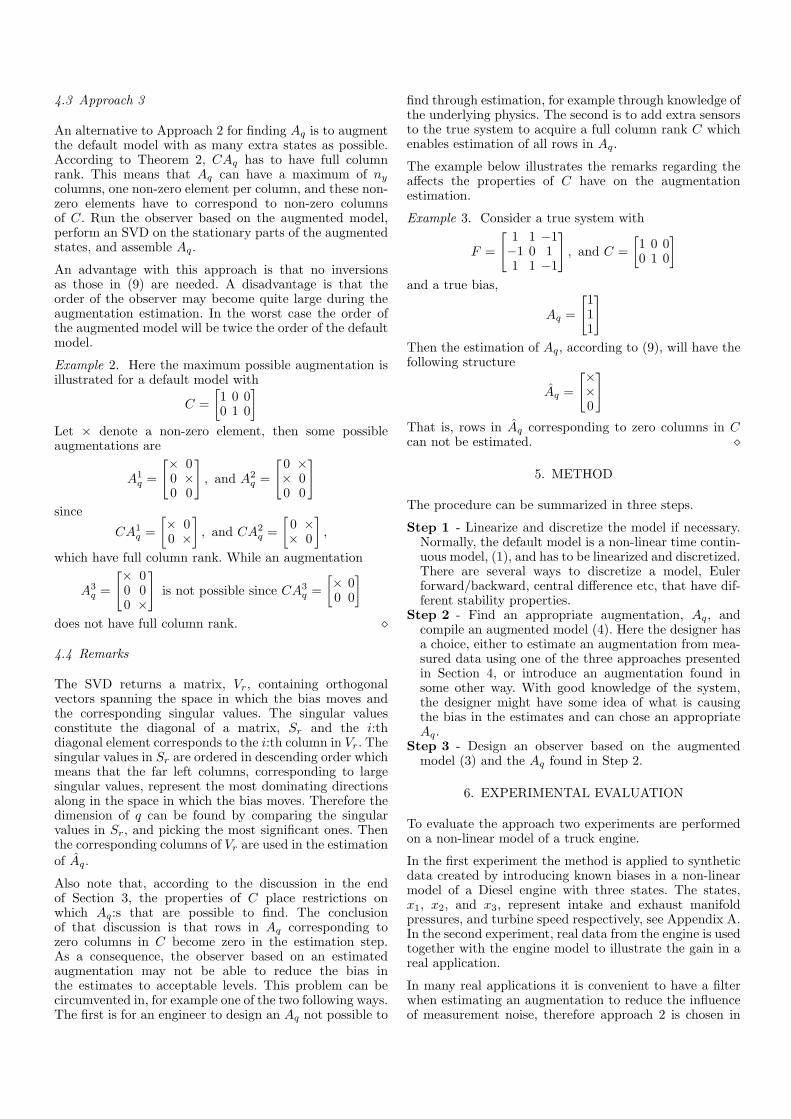
An observer is created using EKF methodology and amodel augmented according to this estimated Aq. Theperformance is compared to the default observer. The stateestimates of x1 and x2 are presented in Figure 1 togetherwith the true states. The reason for not presenting x3 islack of space and that the quality of the estimates arecomparable to the estimates of x1.

It can be seen that the augmented observer estimates x2

better than the default observer while they both seem toestimate x1 equally well.

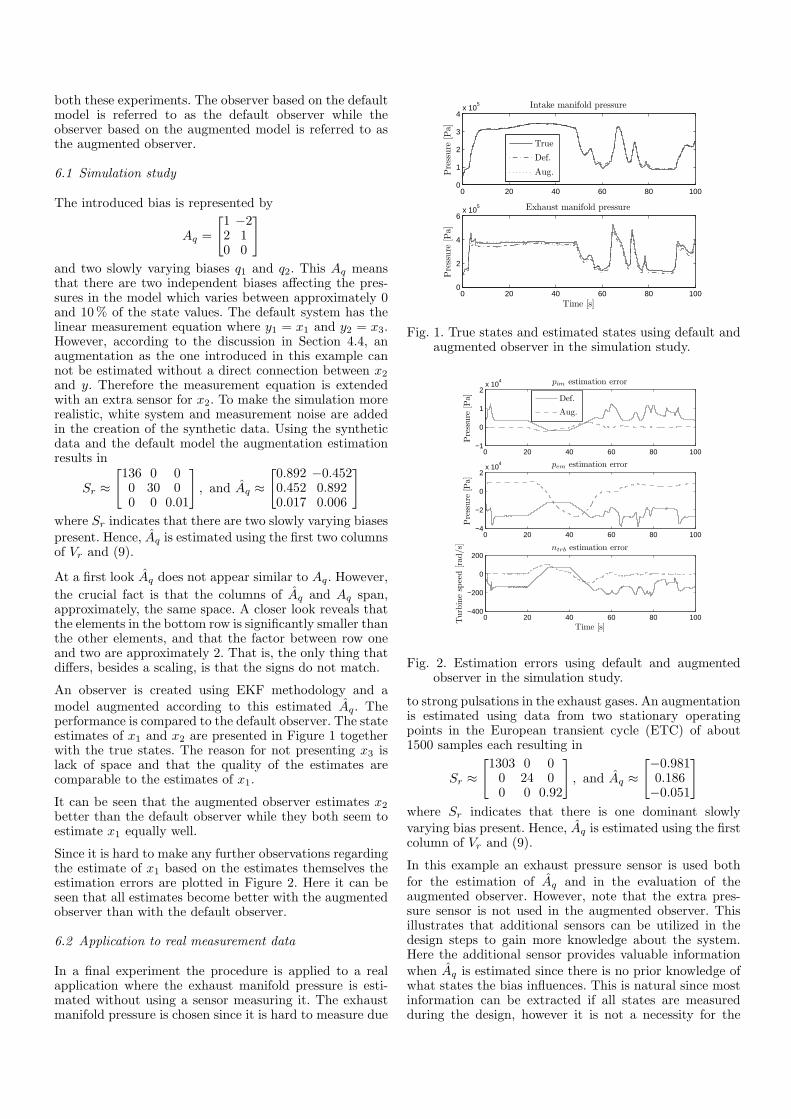
Since it is hard to make any further observations regardingthe estimate of x1 based on the estimates themselves theestimation errors are plotted in Figure 2. Here it can beseen that all estimates become better with the augmentedobserver than with the default observer.

6.2 Application to real measurement data

In a final experiment the procedure is applied to a realapplication where the exhaust manifold pressure is esti-mated without using a sensor measuring it. The exhaustmanifold pressure is chosen since it is hard to measure due

0 20 40 60 80 1000

1

2

3

4x 10

5

Pre

ssure

[Pa]

Intake manifold pressure

0 20 40 60 80 1000

2

4

6x 10

5

Time [s]

Pre

ssure

[Pa]

Exhaust manifold pressure

True

Def.

Aug.

Fig. 1. True states and estimated states using default andaugmented observer in the simulation study.

0 20 40 60 80 100−1

0

1

2x 10

4

Pre

ssure

[Pa]

pim estimation error

Def.

Aug.

0 20 40 60 80 100−4

−2

0

2x 10

4P

ress

ure

[Pa]

pem estimation error

0 20 40 60 80 100−400

−200

0

200

Time [s]

Turb

ine

spee

d[rad

/s]

ntrb estimation error

Fig. 2. Estimation errors using default and augmentedobserver in the simulation study.

to strong pulsations in the exhaust gases. An augmentationis estimated using data from two stationary operatingpoints in the European transient cycle (ETC) of about1500 samples each resulting in

Sr ≈

[

1303 0 00 24 00 0 0.92

]

, and Aq ≈

[

−0.9810.186−0.051

]

where Sr indicates that there is one dominant slowlyvarying bias present. Hence, Aq is estimated using the firstcolumn of Vr and (9).

In this example an exhaust pressure sensor is used bothfor the estimation of Aq and in the evaluation of theaugmented observer. However, note that the extra pres-sure sensor is not used in the augmented observer. Thisillustrates that additional sensors can be utilized in thedesign steps to gain more knowledge about the system.Here the additional sensor provides valuable informationwhen Aq is estimated since there is no prior knowledge ofwhat states the bias influences. This is natural since mostinformation can be extracted if all states are measuredduring the design, however it is not a necessity for the

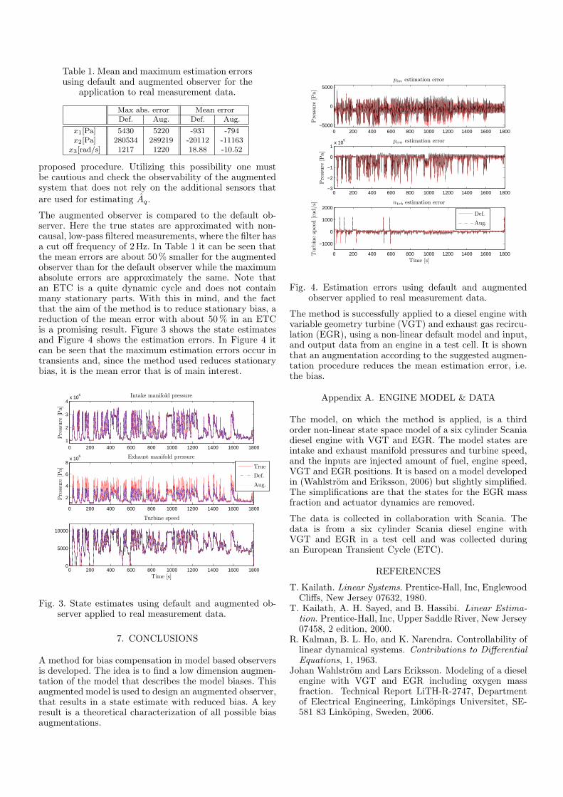
Table 1. Mean and maximum estimation errorsusing default and augmented observer for the

application to real measurement data.

Max abs. error Mean errorDef. Aug. Def. Aug.

x1[Pa] 5430 5220 -931 -794x2[Pa] 280534 289219 -20112 -11163

x3[rad/s] 1217 1220 18.88 -10.52

proposed procedure. Utilizing this possibility one mustbe cautious and check the observability of the augmentedsystem that does not rely on the additional sensors thatare used for estimating Aq.

The augmented observer is compared to the default ob-server. Here the true states are approximated with non-causal, low-pass filtered measurements, where the filter hasa cut off frequency of 2 Hz. In Table 1 it can be seen thatthe mean errors are about 50 % smaller for the augmentedobserver than for the default observer while the maximumabsolute errors are approximately the same. Note thatan ETC is a quite dynamic cycle and does not containmany stationary parts. With this in mind, and the factthat the aim of the method is to reduce stationary bias, areduction of the mean error with about 50 % in an ETCis a promising result. Figure 3 shows the state estimatesand Figure 4 shows the estimation errors. In Figure 4 itcan be seen that the maximum estimation errors occur intransients and, since the method used reduces stationarybias, it is the mean error that is of main interest.

0 200 400 600 800 1000 1200 1400 1600 18001

2

3

4x 10

5

Pre

ssure

[Pa]

Intake manifold pressure

0 200 400 600 800 1000 1200 1400 1600 1800

2

4

6

8x 10

5

Pre

ssure

[Pa]

Exhaust manifold pressure

0 200 400 600 800 1000 1200 1400 1600 18000

5000

10000

Time [s]

Turbine speed

True

Def.

Aug.

Fig. 3. State estimates using default and augmented ob-server applied to real measurement data.

7. CONCLUSIONS

A method for bias compensation in model based observersis developed. The idea is to find a low dimension augmen-tation of the model that describes the model biases. Thisaugmented model is used to design an augmented observer,that results in a state estimate with reduced bias. A keyresult is a theoretical characterization of all possible biasaugmentations.

0 200 400 600 800 1000 1200 1400 1600 1800−5000

0

5000

Pre

ssure

[Pa]

pim estimation error

0 200 400 600 800 1000 1200 1400 1600 1800−3

−2

−1

0

1x 10

5

Pre

ssure

[Pa]

pem estimation error

0 200 400 600 800 1000 1200 1400 1600 1800

−1000

0

1000

2000

Time [s]

Turb

ine

spee

d[rad/s] ntrb estimation error

Def.

Aug.

Fig. 4. Estimation errors using default and augmentedobserver applied to real measurement data.

The method is successfully applied to a diesel engine withvariable geometry turbine (VGT) and exhaust gas recircu-lation (EGR), using a non-linear default model and input,and output data from an engine in a test cell. It is shownthat an augmentation according to the suggested augmen-tation procedure reduces the mean estimation error, i.e.the bias.

Appendix A. ENGINE MODEL & DATA

The model, on which the method is applied, is a thirdorder non-linear state space model of a six cylinder Scaniadiesel engine with VGT and EGR. The model states areintake and exhaust manifold pressures and turbine speed,and the inputs are injected amount of fuel, engine speed,VGT and EGR positions. It is based on a model developedin (Wahlstrom and Eriksson, 2006) but slightly simplified.The simplifications are that the states for the EGR massfraction and actuator dynamics are removed.

The data is collected in collaboration with Scania. Thedata is from a six cylinder Scania diesel engine withVGT and EGR in a test cell and was collected duringan European Transient Cycle (ETC).

REFERENCES

T. Kailath. Linear Systems. Prentice-Hall, Inc, EnglewoodCliffs, New Jersey 07632, 1980.

T. Kailath, A. H. Sayed, and B. Hassibi. Linear Estima-tion. Prentice-Hall, Inc, Upper Saddle River, New Jersey07458, 2 edition, 2000.

R. Kalman, B. L. Ho, and K. Narendra. Controllability oflinear dynamical systems. Contributions to DifferentialEquations, 1, 1963.

Johan Wahlstrom and Lars Eriksson. Modeling of a dieselengine with VGT and EGR including oxygen massfraction. Technical Report LiTH-R-2747, Departmentof Electrical Engineering, Linkopings Universitet, SE-581 83 Linkoping, Sweden, 2006.