DRAFT: May 16, 2015Preprint typeset using LATEX style emulateapj v. 08/13/06

OBSERVING STRATEGY FOR THE SDSS-IV/MANGA IFU GALAXY SURVEY

David R. Law1, Renbin Yan2, Matthew A. Bershady3, Kevin Bundy4, Brian Cherinka5, Niv Drory6, NicholasMacDonald7, Jose R. Sanchez-Gallego2, David A. Wake3,8 Anne-Marie Weijmans9, Michael R. Blanton10, Mark

A. Klaene11, Sean M. Moran12, Sebastian F. Sanchez13, Kai Zhang2

DRAFT: May 16, 2015

ABSTRACTMaNGA (Mapping Nearby Galaxies at Apache Point Observatory) is an integral-field spectroscopic

survey that is one of three core programs in the fourth-generation Sloan Digital Sky Survey (SDSS-IV).MaNGA’s 17 pluggable optical fiber-bundle integral field units (IFUs) will observe a sample of 10,000nearby galaxies distributed throughout the SDSS imaging footprint (focusing particularly on the NorthGalactic Cap). In each pointing these IFUs are deployed across a 3 field; they yield spectral coverage3600-10,300 A at a typical resolution R ∼ 2000, and sample the sky with 2” diameter fiber apertureswith a total bundle fill factor of 56%. Observing over such a large field and range of wavelengthsis particularly challenging for obtaining uniform and integral spatial coverage and resolution at allwavelengths and across each entire fiber array. Data quality is affected by the IFU constructiontechnique, chromatic and field differential refraction, the adopted dithering strategy, and many othereffects. We use numerical simulations to constrain the hardware design and observing strategy for thesurvey with the aim of ensuring consistent data quality that meets the survey science requirementswhile permitting maximum observational flexibility. We find that MaNGA science goals are bestachieved with IFUs composed of a regular hexagonal grid of optical fibers with rms displacement of5 µm or less from their nominal packing position; this goal is met by the MaNGA hardware, whichachieves 3 µm rms fiber placement. We further show that MaNGA observations are best obtained insets of three 15-minute exposures dithered along the vertices of a 1.44 arcsec equilateral triangle; thesesets form the minimum observational unit, and are repeated as needed to achieve a combined signal-to-noise ratio of 5 A−1 per fiber in the r-band continuum at a surface brightness of 23 AB arcsec−2.In order to ensure uniform coverage and delivered image quality, we require that the exposures in agiven set be obtained within a 60 minute interval of each other in hour angle, and that all exposuresbe obtained at airmass . 1.2 (i.e., within 1-3 hours of transit depending on the declination of a givenfield).Subject headings: atmospheric effects, methods: observational, surveys: galaxies, techniques: imaging

spectroscopy

1 Space Telescope Science Institute, 3700 San Martin Drive, Bal-timore, MD 21218, USA (dlaw@stsci.edu)

2 Department of Physics and Astronomy, University of Ken-tucky, 505 Rose Street, Lexington, KY 40506-0055, USA

3 Department of Astronomy, University of Wisconsin-Madison,475 N. Charter Street, Madison, WI, 53706, USA

4 Kavli Institute for the Physics and Mathematics of the Uni-verse, Todai Institutes for Advanced Study, the University ofTokyo, Kashiwa, Japan 277-8583 (Kavli IPMU, WPI)

5 Dunlap Institute for Astronomy and Astrophysics, Universityof Toronto, 50 St. George Street, Toronto, Ontario M5S 3H4,Canada

6 McDonald Observatory, Department of Astronomy, Universityof Texas at Austin, 1 University Station, Austin, TX 78712-0259,USA

7 Department of Astronomy, Box 351580, University of Wash-ington, Seattle, WA 98195, USA

8 Department of Physical Sciences, The Open University, MiltonKeynes, MK7 6AA, UK

9 School of Physics and Astronomy, University of St Andrews,North Haugh, St Andrews KY16 9SS, UK

10 Center for Cosmology and Particle Physics, Department ofPhysics, New York University, 4 Washington Place, New York, NY10003

11 Apache Point Observatory, P.O. Box 59, Sunspot, NM 88349,USA

12 Smithsonian Astrophysical Observatory, 60 Garden Street,Cambridge, MA 02138, USA

13 Instituto de Astronomia, Universidad Nacional Autonoma deMexico, A.P. 70-264, 04510 Mexico D.F., Mexico

1. INTRODUCTION

Integral field spectroscopy (IFS) at optical and infraredwavelengths is among the most significant developmentsin modern observations of galaxies at all redshifts be-cause it combines the benefits of two-dimensional photo-metric analysis with physical diagnostics of baryon com-position and kinematics (e.g., Emsellem et al. 2004; Lawet al. 2009; Bershady al. 2010; Sanchez et al. 2012; Wei-jmans et al. 2014; Fabricius et al. 2014). Recent ad-vances now enable multi-object IFS with instrumentssuch as SAMI (Croom et al. 2012), KMOS (Sharples etal. 2013), and MaNGA (Drory et al. 2015). As a partof the 4th generation of the Sloan Digital Sky Survey(SDSS-IV), the MaNGA (Mapping Nearby Galaxies atAPO) project (Bundy et al. 2015) bundles fibers from theBOSS (Baryon Oscillation Spectroscopic Survey) spec-trograph (Smee et al. 2013) into integral-field units toobtain spatially resolved optical spectroscopy of 10,000nearby galaxies over a 6 year survey. Early results ob-tained with prototype MaNGA hardware (Belfiore et al.2015; Li et al. 2015; Wilkinson et al. 2015) demonstratethe richness of the data for exploring the stellar and gascomposition.

Because current large-format detectors lack energy res-olution throughout most of the electromagnetic spec-

2 Law et al.

trum, IFS has adopted a range of technical approachesto down-selecting and formatting a subset of the three-dimensional data cube of wavelength and spatial positiononto a two-dimensional detector array. These approachesyield different, science-driven trades in the data-cubesampling. Simultaneous and integral coverage of thespatial field is desirable and achieved by a number ofinstruments using lenslets (e.g., SAURON, OSIRIS; Ba-con et al. 2001; Larkin et al. 2003) or image slicers (e.g.,SINFONI, MUSE; Eisenhauer et al. 2003; Bacon et al.2010). However, the two current wide-field, multi-object,IFS instruments–SAMI and MaNGA–use bare-fiber ar-rays to minimize cost while maximizing flexibility andpatrol area, but at the penalty of not achieving truly in-tegral spatial coverage at any one time. This shortfallcan be overcome by careful attention to the interplay ofthe hardware design of the fiber bundles and the observ-ing strategy.

The most immediate challenge is that the MaNGAfiber bundle, composed of circular apertures with largeinterstitial gaps that significantly undersample the PSFat the focal plane of the telescope, has a non-uniform re-sponse across each IFU. This means that (under mosttechniques for the reconstruction of images from thedata) the appearance of objects that are small with re-spect to the fiber size (e.g., AGN or H ii regions) canvary across an IFU. The reconstructed image of such un-resolved objects can either look small and circular (if theobject was centered on a single fiber), large and circular(if the object was centered in the interstitial gap betweenthree fibers), highly elongated (if the object was cen-tered midway between two fibers), along with any rangeof shapes in between.

This is highly undesirable from a science standpoint,and therefore typical fiber-bundle IFU surveys (e.g.,Croom et al. 2012; Sanchez et al. 2012) dither their ob-servations. Small dithers of a fraction of the fiber spac-ing sample the missing points in the image plane andallow reconstructed images based on multiple, ditheredexposures to achieve fairly uniform and integral spatialcoverage.

This dithering is complicated by atmospheric refrac-tion however, especially given the extremely wide spa-tial and spectral coverage of MaNGA. Chromatic dif-ferential refraction over the MaNGA wavelength range(λλ 3600− 10300 A) can be comparable to the diameterof individual fibers, and field differential refraction (fromvariation in the amount and direction of refraction overthe 3 field of an SDSS plugplate) contributes similarly.These effects combine to degrade the effectiveness of aregular dithering scheme in sampling the image plane.

This paper presents simulations that explore the im-pact of these effects on the expected MaNGA data qual-ity, and thereby constrain the hardware design and ob-serving strategy for the survey. In §2 we give an overviewof the SDSS 2.5m telescope and plugplate system, alongwith a brief description of the MaNGA legacy hardwareand IFU ferrule designs considered for the survey. Wedescribe the basic design considerations for the survey in§3. Using the science requirements summarized in §3.1,typical integration times set by the read noise character-istics of our detectors (§3.2), and numerical simulations(§3.3) we motivate the need for dithered observations andregular hexagonal packing of the IFU fiber bundles, cul-

minating in a baseline hardware design and observingstrategy described in §3.4. This baseline observing strat-egy is significantly complicated by atmospheric differen-tial refraction, and we discuss the impact of chromaticand field differential refraction on our data quality in §4.1and 4.2 respectively, defining a uniformity statistic Ω todescribe the data quality in §5. Using the Ω statistic weformulate our final observing strategy in terms of visi-bility windows in §6, noting a few additional practicalconsiderations (e.g., dithering accuracy and IFU bundlerotation) in §7. We summarize our conclusions in §8.

2. OBSERVATORY AND HARDWARE OVERVIEW

2.1. Observatory and Legacy HardwareMaNGA operates on the SDSS 2.5-m telescope (Gunn

et al. 2006) located at Apache Point Observatory (APO;latitude φ = +32 46′ 49′′). The telescope is a modifiedRitchey-Chretien with alt-az mount that is designed withan interchangeable cartridge system that can be installedat the Cassegrain focus. The MaNGA hardware is de-scribed in greater detail by Drory et al. (2015); here webriefly review the major salient features of the system.

MaNGA has 6 cartridges, each of which contains aplugplate with a field of view ∼ 3 in diameter that hasbeen pre-drilled with holes corresponding to the locationsof target galaxies into which optical fibers and IFUs canbe plugged each day in preparation for a night of observ-ing. These plates are fixed at zero degrees position angle(i.e., the on-sky orientation of the telescope focal planecoordinate reference frame is fixed).

Each MaNGA cartridge has a total of 1423 fibers (709on spectrograph 1, 714 on spectrograph 2), correspond-ing to 17 science IFUs ranging in size from 19 to 127fibers (12.5 − 32.5 arcsec diameter; 1247 fibers total),twelve 7-fiber mini-bundles used for spectrophotometiccalibration (84 fibers total; see Yan et al. in prep), and92 single fibers used for sky subtraction that can be de-ployed within a 14’ radius of their associated IFU har-ness.14 Each IFU has its rotation fixed using alignmentpins in the ferrules that plug into corresponding align-ment holes located a short distance West of each targetgalaxy.

These optical fibers feed the twin BOSS (Dawson et al.2013, Baryonic Oscillation Spectroscopic Survey,) spec-trographs (Smee et al. 2013). The collimated beams ineach spectrograph are split with a dichroic and feed ablue (λλ3600−6000 A) and red camera (λλ6000−10300A). The blue cameras use blue-sensitive 4k × 4k e2VCCDs while the red cameras use 4k × 4k fully-depletedLBNL CCDs; all cameras have 15µm pixels. Spectral res-olution varies with wavelength from R = λ/δλ ∼ 1400at 3600 A to R ∼ 2000 at 6000 A (blue channel), andR ∼ 1800 at 6000 A to R ∼ 2200 at 10300 A (red chan-nel; see Fig. 36 of Smee et al. 2013). Spectra fromeach of these four cameras are extracted and processedthrough sky subtraction, spectrophotometric calibration,astrometric registration, and reconstructed into three-dimensional data cubes using a software pipeline (Law

14 The physical size of the hardware components also definesa minimum-distance exclusion zone around each plugged object.These exclusion distances are 116” (7 mm), 89” (5.35 mm), and62” (3.7 mm) for IFU-IFU, IFU-sky, and sky-sky fiber placementrespectively.

MaNGA Observing Strategy 3

32.5’’ 19.7’’

Fig. 1.— Fiber bundle designs considered for MaNGA (whiteregions represent live fiber cores). The left-hand panel shows a 127-fiber bundle for which the fibers are arranged in a regular hexago-nal array (i.e., the final MaNGA IFU design; shown here is as-builtharness ma024); the right-hand panel shows an example bundle of61 fibers in a circular packing arrangement based on that adoptedby the SAMI team for use at the Australian Astronomical Obser-vatory (Croom et al. 2012, compare their Fig. 3). Although thehexagonal arrangement of fibers has greater regularity, the circulararrangement has greater effective filling factor since the protectivebuffers are stripped.

et al. in prep) descended from that previously used forBOSS (idlspec2d; see Bolton et al. 2012, Schlegel et al.in prep)

The telescope guider system is optimized for a wave-length of ∼ 5500 A and uses endoscopic fibers insertedinto 16 holes in each plugplate corresponding to the lo-cations of bright guide stars. These endoscopic fibersproduce images of the guide stars on a guider camera,and the guider actively adjusts the focus, scale, rota-tion, and offset of the telescope focal plane to track thesestars through varying weather conditions and observingangles.

2.2. IFU Ferrule DesignThe ability of an IFU fiber bundle to deliver good, re-

peatable, and uniform image quality depends most fun-damentally on the arrangement of fibers within the bun-dle; while dithering (§3.3.2), differential refraction (§4),and other considerations are important, the fiber place-ment sets the basis for the sampling regularity of theentire survey.

As described by Drory et al. (2015), the MaNGA fibershave an inner light-sensitive core diameter (ID) of 120 µm(corresponding to 2.0 arcsec in the telescope focal plane)and an outer diameter (OD) of 151.0±0.5 µm with theirprotective buffers and cladding. We originally consideredtwo kinds of fiber bundles for MaNGA, as illustrated inFigure 1. The first was a circular bundle of fibers thatmaximizes the filling factor of light-sensitive fiber coresrelative to the total IFU footprint by chemically strippingthe protective buffers from the ends of each fiber. As de-veloped for the SAMI survey by Bland-Hawthorn et al.(2010), these ‘Sydney-style’ bundles maximize the effec-tive filling factor at the cost of decreased fiber throughputdue to focal ratio degradation (FRD), greater fragility ofthe glass cores, and irregular fiber packing due to thecircular ferrule geometry. Based on the numerical per-formance simulations described in §3.3.3, we prototyped(and ultimately chose to adopt) a second style of fiberbundle composed of a regular arrangement of bufferedfibers within a tapered hexagonal ferrule for which wepioneered a novel construction technique (see details in

0 10 20 30Buffer + Clad Thickness (microns)

0.2

0.4

0.6

0.8

1.0

Fill

ing

Fa

cto

r

Fig. 2.— Effective IFU filling factor (live fiber core area dividedby total IFU footprint) as a function of buffer thickness for anideal 127-fiber (solid line) and a 19-fiber (dotted line) hexagonalIFU. The small difference between the solid and dotted lines repre-sents the diminishing importance of edge effects in the hexagonalfootprint as the IFU area increases. The filled star represents themeasured 56% filling factor of the as-built 127-fiber MaNGA IFUs(Drory et al. 2015), which is consistent with theoretical expecta-tions. The filled triangle shows the 75% filling factor of the SAMIsurvey bundles (5 µm cladding) for comparison.

Drory et al. 2015). While reaching lower effective fillingfactor, this technique improves fiber throughput,15 de-creases breakage,16 and (by virtue of its hexagonal geom-etry) permits extremely regular fiber placement withineach IFU.

The theoretical effective fiber packing density of thehexagonal IFUs can be defined as the ratio of the totalfiber core area (Acore) to the area of the hexagon circum-scribing the fiber bundle (Ahex), where:

Ahex =√

32d2(√

3NR + 1)2 (1)

Acore = π

(d− 2t

2

)2

(1 + 3NR(NR + 1)) (2)

Here d = 151 µm is the outer diameter of an individualfiber, t = 15.5 µm is the thickness of the fiber buffer andcladding, and NR is the number of ‘rings’ in the bundle(NR = 2 for a 19-fiber IFU, and NR = 6 for a 127-fiber IFU). In Figure 2 we plot the effective filling factorf = Acore/Ahex as a function of the buffer thickness t.

15 A conservative estimate can be made by comparing Figure 4of Croom et al. (2012) to Figure 11 of Drory et al. (2015): MaNGAachieves 95 ±1 % throughput with an exit f-ratio of f/4 for fibersfed at f/5. In contrast, the original SAMI bundles achieved 50-75% throughput with an exit f-ratio of f/3.15 fed at f/3.4. We notethat the FRD of even the second-generation SAMI bundles (Fig.5 of Bryant et al. 2014) is sufficiently large that it would requireour optics to be 40% larger in area to collect the same ensquaredenergy given the Sloan telescope feed.

16 After ∼ 6 months of operation, 7 individual fibers within IFUshave broken (1 in manufacturing, 1 in assembly, 5 in operation),representing < 0.1% of the total. Detailed statistics on the break-age frequency of stripped, fused fiber bundles are unknown butwould have represented a significant cost increase in manufactur-ing.

4 Law et al.

In accord with these predictions, the prototype circularSydney-style bundles (whose fibers are chemically etchedto an outer diameter of ∼ 132 µm) achieve a filling fac-tor of ∼ 70%, while the as-built hexagonal bundles withfully-buffered fibers achieve a filling factor of 56%.

3. BASIC CONSIDERATIONS

3.1. Required PerformanceSince the fiber bundles consist of 2” diameter circu-

lar apertures separated by large interstitial gaps, eachexposure will significantly undersample the point spreadfunction (PSF) at the focal plane of the telescope (typi-cally ∼ 1.5”) and produce a non-uniform response func-tion across the face of each IFU. We require that theMaNGA IFUs deliver sufficiently uniform performancethat physical structures do not vary in shape as a func-tion of where they happen to fall within the IFU (i.e., acircular star forming region within a galaxy should ap-pear circular in the final MaNGA data cube regardless ofwhether it is in the center or the outskirts of the galaxy).

A convenient way to place a limit on the level of unifor-mity required is to ensure that variations in the 2d PSFof the reconstructed MaNGA data cubes do not signifi-cantly impact measurements of the Balmer decrement orBPT-style (e.g., Baldwin et al. 1981) line ratio diagrams.Since atmospheric differential refraction shifts the effec-tive position of each fiber as a function of wavelength(§4), [O II] and Hα observations of a given H ii regionfor instance will be obtained with a slightly different con-figuration of fibers – while Hα emission may be centeredin a given fiber, spatially coincident [O II] emission maybe centered in the interstitial region between fibers.

As outlined in the MaNGA Science Requirements Doc-ument (SRD; see Yan et al. in prep), relative spectopho-tometry between [O II] (λ = 3727 A) and Hα (λ = 6564A) must be accurate to 7% or better in order to ob-tain the desired constraints on the star formation rate(SFR) and nebular metallicity within galaxies. We there-fore explore how this required spectrophotometric accu-racy translates to limits on the spatial variability of theMaNGA PSF.

We begin by assuming that the PSF in a typicalMaNGA reconstructed data cube can be characterizedby a circular gaussian with a FWHM of 2.5 arcsec (as wediscuss at greater length in Law et al., in prep, this modelis a good approximation to the MaNGA commissioningdata). Using typical aperture photometry techniques, acircular aperture of radius 2.66 arcsec (i.e., 2.5 times theradial scalelength of the PSF) would nominally enclose96% of the total flux.17 In Figure 3 we illustrate how de-viations from the nominal PSF model would affect thistotal; as the PSF becomes broader or more elongatedthe flux contained within the fixed aperture decreases,meaning that the derived aperture-corrected total fluxeswould be in error.18 In particular, we find that an er-ror of 20% in the profile FWHM and 15% in the profile

17 If we were to adopt a PSF model with more power in thewings, or shrink the size of the circular aperture the variabilitybetween different PSF shapes would increase and lead to morestringent constraints on the allowable variability in the deliveryMaNGA PSF.

18 If the goal were to measure the flux from a single bright sourcewhose structure is known a-priori to be effectively a point sourcethen the actual light profile could be measured at each wavelength

Fra

ctio

na

l u

x e

rror

0

0.1

0.2

XFWHM

(arcsec)

YF

WH

M /

XF

WH

M

2.52.0 3.0

1.0

1.5

0.5

Underestimated

Overestimated

7%

Fig. 3.— Fractional error in the recovered flux from a pointsource if the assumed FWHM and axis ratio were incorrect. Thereference source is taken to have a circular gaussian PSF withFWHM 2.5 arcsec; integrating the flux within a 2.5 RMS widthaperture nominally encloses 95.7% of the total flux. If the actualFWHM is smaller (larger) than the model along any dimension thetotal flux enclosed by the aperture increases (decreases), resultingin an overestimate (underestimate) of the total flux. The dashedred line indicates the 7% error threshhold set by the MaNGA SRD;the solid black star indicates our adopted limits on the allowablevariability of the delivered MaNGA PSF (15% in axis ratio, and15% in circularly averaged PSF FWHM).

minor/major axis ratio is sufficient to bias the resultingflux measurements at the 7% level (filled star in Figure3).

Similarly, in order to ensure that our limiting fluxesfor undetected nebular transition features are accurate atthe 7% level we also require that the signal-to-noise ratioof our data is constant at the 7% level across each IFU.Since the limiting flux is proportional to the square rootof the exposure time, this translates to a requirementthat the exposure time is effectively constant across eachIFU at the 15% level.

These three metrics (circularity, FWHM, and signal-to-noise ratio) therefore set our requirements on the uni-formity of the reconstructed image profile such that thecalibrated fluxes derived from MaNGA data cubes areaccurate at the 7% level. Ideally, however, we wouldprefer that spatial sampling issues not dominate the fluxcalibration accuracy budget for the MaNGA data cubes,and we therefore set a goal of achieving photometric per-formance at the 3.5% level where possible. The MaNGAhardware construction, dithering pattern, and observingstrategy is therefore set by the following three high-levelconsiderations:

1. The reconstructed FWHM of all angular resolutionelements in a bundle should vary by < 10% (goal)or 20% (requirement) across each IFU.

2. The reconstructed minor-to-major axis ratio of allresolution elements in a bundle should be b/a ≥0.93 (goal) or 0.85 (requirement) across each IFU.

3. The effective integration time of all resolution ele-ments in a bundle should vary by < 7% (goal) or15% (requirement) across each IFU.

and the aperture adjusted accordingly. However, such a-prioriknowledge of the intrinsic source structure cannot generally beassumed. Similarly, we assume that wavelength-dependant vari-ations from the λ−1/5 Kolmogorov atmospheric turbulence profileare taken into account in determining the appropriate aperture.

MaNGA Observing Strategy 5

3.2. Integration TimeThe total integration time is set by our requirement

that MaNGA reach a signal-to-noise ratio of 5 A−1

fiber−1 in the r-band continuum at a surface brightnessof 23 AB arcsec−2. As described by Wake et al. (inprep.) and Yan et al. (in prep.) the typical integrationtime per plate to reach this target is anticipated to beabout 3 hours in median conditions. In good conditionshowever the required time could be as low as 1.5-2 hours,and for particularly low-latitude fields the required timecould be as much as 4-5 hours. This substantial varia-tion in total exposure time requires an observing strategyflexible enough to accommodate it.

The optimal integration time for individual exposuresis constrained by the MaNGA hardware and typical back-ground sky spectrum at APO. One of the strengths ofMaNGA is the high throughput of the BOSS spectro-graphs shortward of 4000 A, and we therefore integrateeach exposure for long enough that the shot noise fromthe background sky spectrum and detector dark currentexceeds the read noise. The total noise N as a functionof wavelength is given by

N(λ) =√

(fs(λ) + fd n1) t+ n1N2r (3)

where fs(λ) is the background sky spectrum in units ofe− minute−1 per spectral pixel, fd is the dark current ine− pixel−1 minute−1, Nr is the read noise in e− pixel−1,n1 = 3 pixels is the spatial width of a spectrum on thedetector (see discussion by Law et al. in prep), and tis the integration time of an exposure in minutes. Re-arranging Eqn. 3 we find the time tmin required for thecombined sky background and dark current to equal theread noise:

tmin(λ) =n1N

2r

fs(λ) + fdn1(4)

We estimate fs(λ) for a typical MaNGA dark-time ob-servation using commissioning data from all-sky plate7341 (i.e., a calibration plate for which all IFUs targetregions of blank sky) observed on MJD 56693.19 Fol-lowing the data model outlined by Law et al. (in prep),we take the FLUX array of the reduced mgFrame file(in units of flatfielded e− per spectral pixel), multiplyby the SUPERFLAT array to obtain spectra in raw e−

per spectral pixel, and combine ∼ 600 individual fiberspectra to construct an extremely high-precision modelof the background sky. We take the detector read noiseto be Rn = 2.0 (2.8) e− pixel−1, and the dark current tobe 0.033 (0.066) e− pixel−1 minute−1 for the blue (red)camera (see Table 4 of Smee et al. 2013).20

We plot tmin as a function of wavelength in Figure 4,and note that the sky background rapidly dominates overread noise at almost all wavelengths, especially in thevicinity of strong OH atmospheric emission lines in thenear-IR. The upturn in tmin shortward of 4000 A repre-sents the falloff in blue sensitivity of the detectors, but anintegration time of 15 minutes per exposure ensures thatobservations are shot-noise dominated for all λ > 3700A.

19 MJD (Modified Julian Date) 56693 corresponds to February5, 2014.

20 The dark current is typically . 2% of the dark-time sky back-ground signal.

Although an integration time of longer than 15 minuteswould further decrease the contribution of read noise tothe total error budget, such longer integrations are un-desirable because of the cosmic ray event rate recordedby the red-channel detectors. In practice, the maximumintegration time of each exposure is also limited by dif-ferential atmospheric refraction considerations (see §7.2),and we therefore adopt a nominal time of 15 minutes perexposure. Each completed plate will therefore consist of∼ 6− 20 exposures in order to reach the target depth.

3.3. Numerical Simulations3.3.1. Simulation Method

In order to assess the relative performance of differ-ent IFU bundles and observing techniques we perform aseries of numerical simulations designed to test the uni-formity of their response to unresolved point sources (forwhich spatial structure is most pronounced). Adopting aworking box size of ∼ 45× 45 arcsec with simulated pix-els spaced every 0.1 arcsec we first compute the footprintof a given IFU; this defines a mask image for which eachfiber in the IFU is associated with a given set of pixels inthe telescope focal plane that its light-sensitive core sub-tends. We then create an input ‘image’ to be observedby the simulated MaNGA IFUs by convolving a deltafunction by a model of the PSF at the focal plane of theSDSS 2.5-m telescope. This focal-plane PSF is taken tobe the sum of two Gaussian profiles with FWHM θ and2θ respectively (where θ = 1.4 arcsec is the FWHM ofthe median atmospheric seeing profile divided by 1.05)and peak amplitude ratio of 9/1.21 This input image isconvolved with the top-hat fiber mask to determine thetotal amount of light received by each fiber; althoughthe present simulation considers only a single input im-age the technique is immediately generalizable to multi-wavelength input image slices.

We reconstruct a two-dimensional image from the in-dividual fiber fluxes using a flux-conserving variant ofShepards method (inverse-distance weighting) similar tothat used by the CALIFA survey (Sanchez et al. 2012).As part of MaNGA design simulations we explored alter-native methods of image reconstruction such as drizzling(e.g., as adopted by SAMI, see Sharp et al. 2015), thin-plate-spline fits, minimum curvature surface fits, andkriging. As discussed by Law et al. (in prep) the modifiedShepard’s method yielded the best results, and here weadopt the same parameters (e.g., final spaxel scale of 0.5arcsec) as used by the MaNGA Data Reduction Pipeline(DRP) for genuine survey data. The reconstructed imageis fit with a 2d Gaussian model to determine its FWHMand axial ratio; major axis rotation is left as a free pa-rameter.

This exercise is repeated for delta functions locatedin each of the 0.1 arcsec grid squares that lie within thecentral 75% of the IFU fiber bundle footprint (i.e., ignor-ing edge effects from point sources located on the outerring of an IFU), resulting in ∼ 40, 000 simulated points

21 Mathematically, this is equivalent to the linear sum of 9/13times the input image convolved with a Gaussian of FWHM θ plus4/13 times the input image convolved with a Gaussian of FWHM2θ. This profile provides a reasonable approximation of the on-axisSDSS focal plane PSF, matching the inner parts of the profile welland accounting for most of the flux in the outer wings (J.E. Gunn,priv. comm.).

6 Law et al.

4000 6000 8000 10000Wavelength (Angstroms)

0

5

10

15

20

Tim

e (

Min

ute

s)

Red cameraBlue camera

Fig. 4.— Exposure time tmin required for a typical MaNGA dark-time sky spectrum to be dominated by Poisson noise from thebackground sky plus detector dark current. The break around 6000 A represents the dichroic break between red and blue channels; inreality there is a ∼ 300 A overlap between these channels. Strong features longwards of ∼ 8000 A are due to bright OH sky lines. Thedashed line indicates the adopted 15 minute exposure time.

across a 127-fiber IFU bundle. In Figure 5 (top row) weplot the on-sky footprint of a hexagonal fiber array, alongwith the variations in effective exposure time (exposuretime multiplied by the fraction of the total light that iscollected by fibers rather than being lost to interstitialregions), FWHM, and minor-to-major axis ratio of thereconstructed point spread function (PSF) as a functionof the location of the point source within the fiber bun-dle. As anticipated, we note that all three quantities varysubstantially across a given IFU in a single exposure.

We quantify these results by calculating the RMS ofthe distributions in effective exposure time and recon-structed PSF FWHM (relative to the median values as[X − Xmedian]/Xmedian), the 3σ width W99 encompass-ing 99% of these values, and the 99% lower bound forthe minor-to-major axis ratio. For a single exposure, theeffective integration time varies by W99 = 30.7% aroundthe median22 value; unsurprisingly, the greatest fractionof the total light is recorded for objects that are centeredin a fiber, while the least amount is recorded for objectsin interstitial regions. Similarly, the reconstructed PSFFWHM varies by almost 80% (from ∼ 2 to 4 arcsec) de-pending on where a source falls with respect to the fibergrid, and the minor-to-major axis ratio b/a of the recon-structed image varies from ∼ 0.5 − 1.0 (99% of valuesb/a ≥ 0.53).

In practical terms, this means that an unresolved H iiregion observed with such an IFU for just a single expo-sure may appear to be compact and circularly symmet-ric if it lands directly in the middle of a fiber, elongatedand skinny if it falls directly between two fibers, or largeand triangular if it falls midway between three adjacentfibers.23 Allowing for the effects of chromatic differentialrefraction (§4.1), this means that a single such H ii regionmay simultaneously be sampled by all three different suchconfigurations at different wavelengths.

3.3.2. Dithering

22 The median effective exposure time is just the filling factor(0.56) times the actual exposure time.

23 Strictly, a single exposure simply does not have the spatialsampling in these cases to discriminate (for instance) between anunresolved point source and an elongated source.

The sampling irregularities from fiber-bundle IFUswith substantial interstitial light losses are well knownfrom previous IFU surveys (e.g., Sanchez et al. 2012;Sharp et al. 2015), and can be largely overcome byobtaining dithered observations. The geometry of thehexagonal fiber arrangement readily lends itself to a fixedtriangular three-point dithering scheme that effectivelyfills the interstitial regions as illustrated in Figure 6. Re-peating the simulations performed in §3.3.1 with suchdithered observations, we find that the combined datafrom just three exposures is able to achieve remarkablyuniform image quality at all locations within a single IFU(Figure 5, bottom row). In contrast to the unditheredcase, 3-point dithering delivers effective exposure timeconstant to within 0.3% RMS, FWHM of 2.69±0.01 arc-sec, and ellipticity ≤ 0.04. This uniformity easily meetsthe MaNGA science requirements described in §3.1.

Logically, the 3-point dithering pattern could be ex-panded to a regular 9-point pattern that also providesuniform coverage of the interstitial gaps, but with a finersampling of the image plane. Although simulations sug-gest that this could provide ∼ 10% improvement in thedelivered PSF FWHM, such gains were not realized on-sky in tests with the MaNGA prototype hardware. Thislack of improvement with respect to theoretical calcula-tions is likely due to a confluence of numerous complicat-ing factors, including degradation of the nominal dither-ing pattern by atmospheric refraction (see §4), variationsin fiber-to-fiber sensitivity, and changes in seeing andtransparency conditions between exposures (see §6.2).

3.3.3. Fiber Packing Regularity

The gains achievable with such dithering depend fun-damentally on the uniformity of each IFU fiber bundleso that a single telescope offset can simultaneously dithereach of our 29 IFUs (17 science and 12 calibration bun-dles) across the 3 field such that their fibers align withthe interstitial gaps from the previous exposure. If fibersare not located at regular positions within every IFU,the dithering will not be able to uniformly sample theimage plane. We explore the effect of fiber packing ir-regularity by repeating our earlier simulations with theintroduction of a random perturbation to the position ofeach fiber in the simulated IFU fiber bundle, such that

MaNGA Observing Strategy 7

Areal Footprint Relative Exp Time Relative PSF FWHM Axis Ratio

0%-20% +20% 0%-50% +50%0 0.5 1.0 0.5 0.75 1.0

σ = 8.3 %

W99

= 30.7 %

σ = 28.4 %

W99

= 79.8 % (b/a)99

≥ 0.53

σ = 0.3 %

W99

= 1.2 %

σ = 1.0 %

W99

= 5.1 % (b/a)99

≥ 0.96

Undithered

Dithered

Fig. 5.— Simulations of point-source response as a function of location within an IFU for a single exposure (top row) and a dithered setof exposures (bottom row) using a theoretically perfect hexagonal fiber bundle. The left-most panels show the footprint of the IFU fiberson the sky, the second column of panels show the percentage variations about the median exposure time as a function of position withinthe bundle. The third column of panels shows the deviation from the median delivered PSF, and the right-hand column of panels showsthe recovered minor/major axis ratio. For undithered observations the greatest effective depth is obtained for sources located in the middleof a fiber (as is the smallest and most circular reconstructed image of a point source), while point sources falling in interstitial regionsbetween fibers have minor/major axis ratios as low as ∼ 0.5 and FWHM nearly double that of sources centered within a fiber. Numbers inpanels 2-4 indicate the RMS deviation between values (σ), the 3σ width encompassing 99% of all values (W99), and the minor/major axisratio above which 99% of point lie ((b/a)99).

N

E

ON-SKY VIEW

a = 86.6 μm = 1.44’’

b = 50.0 μm = 0.83’’

S

E

N

a

b

C

75 μm

60 μm

Fig. 6.— Schematic diagram of the 7 central fibers within a hexagonally-packed MaNGA IFU, showing the 120 micron diameter fibercore and surrounding cladding plus buffer. The triangular figure shows the relative positions of the three dither positions; the fiber bundleis located at position ‘S’. The central (C) ‘home’ position is labeled, along with the north (N), south (S), and east (E) dither positions.The nominal plate scale of the SDSS telescope is 217.7358 mm/degree, or 60.48 microns/arcsec.

8 Law et al.

each fiber is slightly offset from its nominal position bysome distance drawn randomly from a Gaussian distri-bution with a given rms. Each simulated IFU bundle isobserved with a nominal 3-pt dither pattern as defined byFigure 6. Additionally, we simulate the effect of observ-ing the circular Sydney-style fiber bundle with a 7-pointdither pattern (based on that adopted by the SAMI sur-vey) that compensates for the irregular fiber placementwith greater filling factor and a larger number of ditheredsampling points.

As indicated by Figure 7, neither the dithered Sydney-style circular fiber bundle nor the 20 µm tolerance hexag-onal fiber bundles meet our target regularity goals, witha recovered PSF FWHM24 varying by > 20% over theextent of an IFU (i.e., 2.66±0.12 arcsec with 99% valuesranging from ∼ 2.3 - 2.9 arcsec), and minor/major axisratios as low as b/a ∼ 0.8. In contrast, using a hexag-onal fiber array constructed to a tolerance of 5 µm rmswith a 3-point dither pattern we expect to achieve a PSFFWHM that varies by less than 10% over a given IFU.

As detailed by Drory et al. (2015), the as-built MaNGAfiber bundles meet and exceed our target threshold witha typical fiber placement accuracy of 3 µm rms. Usingthe as-measured fiber metrology25 for 127-fiber MaNGAbundle ma024, we simulate the anticipated performanceusing this fiber bundle in row E of Figure 7. With a nom-inal dither pattern we expect to achieve a PSF FWHMwhich varies by less than 7% over an IFU (i.e., 2.66±0.01arcsec with 99% values ranging from ∼ 2.6 to 2.7 arc-sec), and has a nearly circular profile everywhere withb/a > 0.95.

3.4. Baseline Observing StrategyThe dithered observing simulations presented in §3.3.2

and exposure time requirements described in §3.2 mo-tivate a nominal observing scheme in which targets areobserved in sets of 3 dithered exposures (N-S-E) of 15minutes each. Given the regularity of fiber placementwith each IFU and the locator pins that constrain eachIFU to have the same position angle, correctly-ditheredexposures can be simultaneously obtained for all IFUs ona given plate by simply offsetting the telescope pointingwith respect to the guide stars. Since the coverage andimage quality of a single set of three dithered exposuresis known to be acceptably uniform, the total summedcoverage of N such sets will also be uniform and havea depth of 0.75N hours, allowing us to simply observeadditional sets of 3 exposures until the combined datareaches our target signal-to-noise ratio of 5 A−1 fiber−1

in the r-band continuum at a surface brightness of 23 ABarcsec−2.

Such a scheme provides us with considerable flexibil-ity to adjust our total exposure time in 45-minute in-crements without adversely impacting the delivered dataquality whether there are 6 or 20 total exposures for agiven galaxy. It is this flexibility as much as the ditheredperformance simulations themselves that drives us toadopt the regular hexagonal fiber arrays for MaNGArather than the SAMI-style circular fiber bundles, which

24 We quote the average of the minor- and major-axis FWHMvalues.

25 The final placement of individual fibers within an IFU can bemeasured to an accuracy of better than 1 µm (Drory et al. 2015).

rely upon a large number of exposures at many differ-ent dither positions to statistically fill in the interstitialgaps.26 However, since this technique relies upon tightlycontrolling the fiber locations to provide uniform cover-age we must properly mitigate a variety of effects thatwill act to degrade this uniformity, and this goal in turndrives many aspects of the survey operation.

4. ATMOSPHERIC REFRACTION

As a photon passes through the Earth’s atmosphere itis refracted by variations in the density of the air. Un-der the usual assumption of a plane-parallel atmospherewith a vertical density gradient this bends the light froman astronomical target along the parallactic angle (thegreat circle connecting the target and the observers localzenith), causing astronomical objects to appear slightlyhigher in the sky than they truly are. Atmospheric re-fraction introduces significant optical distortions that ad-versely affect our ability to dither our IFU observationsto the desired accuracy. Loosely speaking, the effects canbe split into chromatic differential refraction and fielddifferential refraction which we detail below.

4.1. Chromatic Differential RefractionAtmospheric refraction is a function of atmospheric

conditions (temperature, pressure, and relative humid-ity), zenith distance (i.e., the amount of atmospherethat an incoming photon must traverse), and wavelength.The impact of such refraction on astronomical observa-tions has been studied at some length in the literature(e.g., Filippenko 1982; Cuby et al. 1998, and referencestherein); we adopt estimates of the magnitude of refrac-tion r at a given wavelength relative to a fixed ‘guide’wavelength developed by Enrico Marchetti for ESO.27The direction of the refraction is along the local altitudevector for a given star; this corresponds to the parallacticangle η defined by the spherical triangle with vertices atthe star, the celestial pole, and the local zenith.

tan η =sinh cosφ cos δ

sinφ− sin δ cos z(5)

where h is the hour angle (h > 0 towards the West),φ is the local latitude (φ = 32 46′ 49′′ for APO), δ isthe target declination, z is the zenith distance cos z =sinφ sin δ+ cosφ cos δ cosh, and η is defined in the range−180 to +180.

The SDSS 2.5-m telescope is equipped with an alt-az mount and all plates are observed with a positionangle of 0, so the amount of refraction in focal-planecoordinates28 is given by

∆xfocal = −r sin η (6)

∆yfocal = −r cos η (7)

26 Additionally, the hexagonal tapered ferrule construction tech-nique can be scaled up to bundles with large numbers of hexagonal‘rings’ without significantly degrading the packing regularity.

27 See http://www.eso.org/gen-fac/pubs/astclim/lasilla/diffrefr.html

28 SDSS xfocal/yfocal coordinates are defined such that +xfocalcorresponds to +right ascension and +yfocal corresponds to+declination.

MaNGA Observing Strategy 9

Areal Footprint Relative Exp Time Relative PSF FWHM Axis Ratio

F

E

D

C

B

A

0%-20% +20% 0%-10% +10%0 0.5 1.0 0.7 0.85 1.0

σ = 1.4 %

W99

= 7.4 %

σ = 1.3 %

W99

= 6.5 % (b/a)99

≥ 0.95(ma024 as built)

σ = 20 μm

σ = 10 μm

σ = 5 μm

σ = 0 μm

σ = 3 μm

σ = 0.3 %

W99

= 1.2 %

σ = 1.0 %

W99

= 5.1 % (b/a)99

≥ 0.96

σ = 3.0 %

W99

= 13.8 %

σ = 4.2 %

W99

= 20.1 % (b/a)99

≥ 0.83

σ = 11.2 %

W99

= 52.6 %

σ = 4.5 %

W99

= 23.9 % (b/a)99

≥ 0.83

Circular hexabundle

σ = 5.8 %

W99

= 28.0 %

σ = 2.5 %

W99

= 12.8 % (b/a)99

≥ 0.90

σ = 2.9 %

W99

= 14.4 %

σ = 1.5 %

W99

= 7.4 % (b/a)99

≥ 0.94

Fig. 7.— As Figure 5, but showing simulated point-source response as a function of location in an IFU for dithered observations of fiberbundles built to a variety of specifications. Row A simulates a Sydney-style 61-fiber bundle using a 7-point dither pattern. Rows B-Fsimulate a 3-point dither pattern applied to a hexagonal arrangement of 127 fibers with varying RMS deviations of each fiber from thenominal position (σ = 0− 20 µm). Note that for display purposes panel A is zoomed in slightly compared to panels B-F. In order to meetour uniformity criteria we require σ < 5 µm, which our as-built IFUs achieve (row E).

10 Law et al.

Fig. 8.— Differential atmospheric refraction in arcsec of altituderelative to 5500 A for the MaNGA wavelength range as a func-tion of zenith distance. Calculations assume median conditions forAPO with air temperature 10.5 C, 24.5% relative humidity, andatmospheric pressure of 730 mbar.

i.e., at transit h = 0, η = 0, and hence the entirety ofthe apparent refraction is along the yfocal direction.29

Since differential refraction (particularly shortward of4000 A) can be substantial compared to the fiber radiusof 1 arcsec (see Figure 8) the spectrum recorded by asingle fiber is not strictly the spectrum of a single regionin a given galaxy; it is a bent ’tube’ that traces differ-ent regions of the galaxy at different wavelengths. Mostimmediately, this means that the effective on-sky foot-print of the MaNGA IFUs can be shifted by up to ∼ 1arcsec between blue and red wavelengths, requiring thatthe MaNGA data reduction pipeline (DRP; see Law etal. in prep) rectify the spectra to a common astrometricgrid when reconstructing the data cubes. More prob-lematically, since the three exposures in a given ditherset will be obtained at different hour angles the relativeoffset at a given wavelength will change between thesethree exposures and degrade the intended dither patterncoverage.

At the guide wavelength of 5500 A, the three ditherswill be executed properly. As illustrated in Figure 9 how-ever, at other wavelengths there will be variable shifts ofthe effective dithering pattern. These shifts can in somecases be comparable to the dither distances themselves,thereby degrading the effective dither pattern such thatentire dither postions can be effectively ‘lost’ at certainwavelengths. As suggested by Figures 5 and 7 this pro-duces substantial and undesirable non-uniformities in thereconstructed image depth and recovered FWHM profileacross the face of each IFU.

4.2. Field Differential RefractionIn addition to varying with wavelength, both the mag-

nitude and the direction of atmospheric refraction varyaccording to the location of an object on the sky, and

29 In the present work we neglect the relatively small effect ofdistortions introduced by the SDSS 2.5m optical system; these are,however, accounted for in the actual data pipeline described byLaw et al. (in prep).

the 3 SDSS plugplate field over which our IFUs are dis-tributed is sufficiently large that this variation cannot beneglected. As a given field rises, transits, and sets, theapparent locations of astronomical targets in the tele-scope focal plane shift. As described in §2, the SDSStelescope guider system compensates for this using guidefibers placed on astrometric standard stars distributedthroughout a given field, and adjusts the overall shift,rotation, and scale of the focal plane to compensate.However, since field compression occurs along only a sin-gle direction (altitude) it cannot be fully corrected by aglobal change in the focal plane scale, leaving a resid-ual quadrupole term in the guider-corrected focal planelocations of the target galaxies (see Figure 10).30

Such field differential effects are most noticeable whenobserving with single fibers or an array of slits (see, e.g.,discussion by Cuby et al. 1998, for the 16’ x 16’ VI-MOS field of view) since targets can rapidly shift outof the aperture. Hence, previous generations of SDSSthat have used single fiber spectroscopy have been care-ful to observe at hour angles close to that for which agiven plate is drilled. In contrast, MaNGA is relativelyinsensitive to shifts in the effective centroid of an IFUsince such shifts are small compared to the total field ofview of each IFU (∼ 30 arcsec for the 127-fiber IFUs).31The MaNGA plugplates are therefore all drilled for tran-sit (h = 0 hours), so the holes into which the MaNGAIFUs are inserted correspond to the expected focal planelocations of the galaxies at this point in time.

More important for MaNGA is the change in field dif-ferential refraction between exposures in a given ditherset, which leads to degradation of the effective ditherpattern akin to what was seen for chromatic differentialrefraction in Figure 9. As illustrated by Figure 10, themagnitude of this effect depends on the field declination,the hour angle h of exposures within a given set, andthe location of an IFU within the plugplate. In the ex-treme example shown in Figure 10 (low declination, withexposures obtained many hours apart) the shift can becomparable to a fiber diameter. In more realistic andtypical cases (field center at δ = +40, observed at h = 0and h = +1 hours) the shift after guider corrections istypically . 0.1 arcsec.

5. THE UNIFORMITY STATISTIC Ω

Given the presence of both chromatic and field differ-ential refraction, no two exposures taken by MaNGA willhave an identical fiber sampling pattern even in the ab-sence of dithering. The primary driver of the MaNGAobserving strategy is therefore mitigation of the impactof atmospheric differential refraction on the regularity ofthe dither pattern in order to achieve maximally-uniformdata quality and depth within a given IFU.

Given any two exposures separated by a time ∆t thereare vectors ~r1 and ~r2 defining the effective offset of a fiberfrom its intended location on the target galaxy due to

30 Field differential refraction is calculated using the SDSS platedesign code located on the collaboration SVN repository.

31 This effect is more important for the spectrophotometric mini-bundles which have a diameter of only 7.5 arcsec; as discussed byYan et al. (in prep), large offsets of the spectrophotometric stan-dard stars from the center of the calibration minibundles due toa combination of differential refraction, dither offsets, and othereffects can complicate flux calibration.

MaNGA Observing Strategy 11

Coverage pattern: 5500 Å Coverage pattern: 3500 Å

N

S

E

Ω

Fig. 9.— Illustrative figure showing degradation of the intended dither pattern due to chromatic differential refraction. In this examplewe assume a target at δ = +60 was observed with a standard N-S-E dither pattern, but the three exposures were taken at hour anglesh = −4h, 0h, and +4h respectively (corresponding to parallactic angles η = −97, 180,+97). The image on the left shows the offset dueto chromatic refraction at 3500 A relative to the nominal center of a given fiber and defines the regularity statistic Ω. While the achieveddither pattern is nominal at the guide wavelength (central panel), at 3500 A the fibers in positions S and E lie almost atop each other(right panel).

-400 -200 0 200 400Xfocal (mm)

-400

-200

0

200

400

Yfo

ca

l (m

m)

Fig. 10.— Magnified illustration of the effects of field differen-tial refraction at the guide wavelength (∼ 5500 A) across the 3

diameter SDSS plugplate. Black ‘+’ symbols indicate the nominalpositions in focal plane coordinates of a randomly-selected set of 30target galaxies. These locations are computed assuming that theplate center has declination +7 and is observed at transit (h = 0hours); these correspond to the locations of the physically drilledholes in the plugplate into which the MaNGA IFUs are inserted.If the same plate were observed 4 hours later (h = +4 hours) theapparent locations of the galaxies in the focal plane would be dif-ferent due to field differential refraction both before (red asterisks)and after (green open boxes) guider corrections have been applied.Note that all offsets from the nominal positions have been magni-fied by a factor of 300 to enhance visibility; the maximum actualshift after guider corrections in this example is ∼ 2 arcsec.

chromatic differential refraction, and ~s1 and ~s2 the offsetdue to uncorrectable field differential refraction effects.In our rectilinear focal-plane coordinate system the totalshifts from differential refraction are given by:

∆x1 = r1 sin η1 + ~x · ~s1 (8)∆y1 = r1 cos η1 + ~y · ~s1 (9)∆x2 = r2 sin η2 + ~x · ~s2 (10)∆y2 = r2 cos η2 + ~y · ~s2 (11)

where η1 and η2 are the respective parallactic angles forthe two exposures and the vectors ~s1 and ~s2 are eachprojected into their components along the x/y focal planecoordinate system. The quantity of interest for survey

planning purposes is the total distance between theseshifted locations in the focal plane:

Ω =√

(∆x1 −∆x2)2 + (∆y1 −∆y2)2 (12)

In practice, we calculate Ω between the first and lastexposures in a dithered set of three frames (see illus-trative diagram in Figure 9).32 Using the tools devel-oped in §3.3 we simulate four test cases where Ω rangesfrom 0 to 1”. We use the as-built MaNGA 127-fiberIFU ma024, and assume a standard three-point (N-S-E)dithering strategy in which exposure N is shifted by Ω/2in the -Xfocal direction, exposure S is shifted by Ω/3 inthe -Yfocal direction and exposure E is shifted by Ω/2in the +Xfocal direction (see, e.g., Figure 9). Note thatwe are free to assume such symmetry because any shiftcommon to all three exposures will simply result in atranslation of the entire pattern.

We show results for the expected exposure time, re-constructed PSF FWHM, and reconstructed axis ratiouniformity as a function of Ω in Figure 11.33 Figure12 suggests that so long as Ω . 0.2 arcsec observationsshould meet the target uniformity criteria outlined in§3.3.3 with FWHM 2.65±0.08 arcsec. At Ω = 0.4 arcsec,degradations in the reconstructed PSF uniformity andcircularity start to become apparent; although the meanreconstructed PSF in the bundle has FWHM 2.65± 0.14arcsec the total spread of FWHM values can be as largeas ∼ 0.3 arcsec, and 99% of locations have minor/majoraxis ratio greater than 0.85. By Ω = 1.0 arcsec the ditherpattern is badly degraded, with reconstructed FWHMvalues varying by over an arcsecond depending on wherea point source falls within the bundle. Our science re-quirements (§3.1) therefore translate to a requirementthat Ω < 0.4 arcsec, with the goal of reaching Ω < 0.2arcsec for the majority of observations so that it does notdominate the flux calibration accuracy budget.

32 Each exposure is 15 minutes in length; we adopt the mid-point of each exposure as the characteristic instant for purposes ofcalculating Ω (although see §7.2).

33 Note that while Ω degrades the expect coverage pattern, weassume that the magnitude and direction of all of these shifts areknown (see discussion by Law et al. in prep) and the true effectivelocations of each fiber are used when reconstructing the data cube.

12 Law et al.

Areal Footprint Relative Exp Time Relative PSF FWHM Axis Ratio

D

C

B

A

0%-20% +20% 0%-20% +20%0 0.5 1.0 0.7 0.85 1.0

σ = 1.4 %

W99

= 7.4 %

σ = 1.3 %

W99

= 6.5 % (b/a)99

≥ 0.95

Ω = 0.0’’

σ = 1.6 %

W99

= 8.1 %

σ = 2.8 %

W99

= 12.3 % (b/a)99

≥ 0.91

Ω = 0.2’’

σ = 2.3 %

W99

= 10.9 %

σ = 5.3 %

W99

= 22.0 % (b/a)99

≥ 0.85

Ω = 0.4’’

σ = 4.3 %

W99

= 18.5 %

σ = 11.9 %

W99

= 44.2 % (b/a)99

≥ 0.72

Ω = 1.0’’

Fig. 11.— As Figure 5, but showing simulated point-source response variability as a function of location in an IFU for ditheredobservations of MaNGA 127-fiber bundle ma024 with different values of the pattern degradation Ω.

6. MANGA OBSERVING STRATEGY

6.1. Set Lengths and Visibility WindowsAs described above, Ω is a complicated function of

wavelength, integration time, target declination, hourangle, and location of an IFU on a given plate. How-ever, it is possible to define a series of relatively simpleobserving guidelines that will ensure that Ω stays belowour 0.4 arcsec threshold.

First, we note that Ω behaves nearly linearly with theamount of elapsed time between exposures in a given set,meaning that it is desirable to obtain all three exposuresin the set as close in time to each other as possible. Sinceeach exposure is 15 minutes long, we therefore requirethat all three exposures be obtained in a set length ofone hour (i.e., the change in hour angle between the startof the first exposure and the end of the last exposureshould be 1 hour or less, corresponding to 45 minutes

between the effective midpoint of the first and last expo-sure). While we expect that each set of three exposureswill typically last 48 minutes accounting for typical read-out times and overheads, this hour-long block providesnecessary flexibility in scheduling, especially during vari-able weather conditions.

We next calculate the expected Ω within a 1-hour longset as a function of the midpoint hour angle hset of theset (hset denotes the absolute value of the hour anglemidway between the start of the first and end of the lastexposure). In Figure 12 we show the results of this cal-culation for three different wavelengths, three locationson a plate, and a range of different declinations.34 As

34 Due to symmetries inherent in this exercise (chromatic andfield differential effects combining constructively or destructively),at fixed wavelength one side of the plate will exhibit the worst Ω atpositive hour angles (west of meridian) and the other at negativehour angles (east of meridian). For convenience we collapse the

MaNGA Observing Strategy 13

3600 Å 5500 Å 9000 Å

0.0

º o

set

1.0

6º o

se

t1

.5º o

se

t

Fig. 12.— Ω statistic as a function of midpoint hour angle of the set (hset) for a range of wavelengths, target declinations, and locationson a plate. Left, middle, and right columns respectively show results for wavelengths of 3600, 5500, and 9000 A; top, middle, and bottomrow respectively show results for an IFU in the middle of the plate, 1.06 towards the E edge of the plate (a circle at this radius encloses50% of the plate area), and on the E edge of the plate. Red, orange, green, blue, black, and grey solid lines respectively indicate resultsfor declinations δ = 0, 15, 30, 45, 60, and 75. The horizontal dotted lines at Ω = 0.2 and 0.4 indicate the thresholds of ideal andacceptable performance respectively. High-frequency structure in some lines is due to discrete changes in the best-fit guider correctionsbetween individual simulation points.

expected, Ω is largest at extremely blue wavelengths (forwhich chromatic differential refraction is greatest) andon the edges of a plate (where uncorrected field differ-ential refraction is greatest). More importantly however,we note that Ω grows rapidly with increasing hour an-gle (either East or West of the meridian) meaning thatwe want to obtain our observations as close to transit aspossible. Our Ω limit therefore equates to defining a se-ries of visibility windows around transit within whichall MaNGA observations must be taken.

In order to compute the length of these visibility win-dows we require that Ω must be less than 0.4 arcsec forall sets, at all wavelengths, at all locations on a givenplate, and at all declinations. As indicated by Figure

problem such that hset refers to the absolute value of the hourangle, and Ω is taken to be the greater of the value from ±hset.

12, the worst wavelength for Ω will be 3600 A, wherethe chromatic refraction is greatest. We work out theworst location on a given plate as a function of declina-tion by using Monte Carlo techniques to compute Ω foreach of 20,000 randomly chosen locations on an SDSSplugplate over the course of a 1-hour set. As illustratedby Figure 13, the worst Ω is typically for IFUs locatedon the Eastern/Western edges of the plate for targetdeclinations ∼ +30 − 40; this pattern shifts at morenortherly/southerly declinations.

Using these simulations we finally have all of the piecesrequired to define our visibility windows. For a gridof declinations spaced every 5 from δ = 0 to 70 wecompute the limiting set hour angle such that Ω = 0.4arcsec at λ = 3600 A at the worst location on a givenplate. Converting the set midpoint hour angle to themaximum midpoint hour angle of an individual exposure

14 Law et al.

-1.5 -1.0 -0.5 0.0 0.5 1.0 1.5

-1.5

-1.0

-0.5

0.0

0.5

1.0

1.5 0.5

0.4

0.3

0.2

0.1

0.0

Ω (a

rcsec)

Δ R.A. (degrees)

0.0-1.0 1.0

0.0

-1.0

1.0

Δ D

ecl

. (d

eg

ree

s)

Fig. 13.— Ω as a function of location on a plate centered atδ = 40. Simulations are performed at 3600 A and assume a 5-hour observing window (i.e., hset = 2.5 hours either side of transit).Each point represents the maximum value of Ω experienced at agiven location for a hour-long set of exposures taken within thisobserving window (for one side of the plate this maximum willoccur prior to transit, for the other side it will occur after transit).

0 20 40 60Declination (degrees)

0.0

0.5

1.0

1.5

2.0

2.5

3.0

Ho

ur

An

gle

(h

ou

rs)

AM=1.05

AM=1.30

Fig. 14.— Black asterisks show the maximum hour angle awayfrom transit (hexp) within which all MaNGA exposures must beobtained as a function of declination based on numerical simula-tions. The solid black line represents a polynomial fit to these 15data points. Dotted lines indicate contours of constant airmass(every 0.05 from AM 1.05 to 1.30) as a function of declination andhour angle; note that these contours closely track the derived hourangle limits.

(hexp = hset + 22.5 minutes for 1-hour sets), we show thefinal visibility windows as a function of declination inFigure 14. These windows range from about 1h eitherside of transit for fields near the celestial equator to ∼ 3hours for declinations δ ∼ +40.

Intriguingly, despite all of the complications involvedin computing these visibility windows they are nearlyequivalent to simple airmass limits, independent of fielddeclination. As illustrated by Figure 14, our visibilitywindows can be described as a 6th order polynomial asa function of declination, or more simply by the require-ment that airmass AM < 1.21 for all exposures at all de-clinations. This airmass limit is determined by the SDSSplate diameter, the BOSS spectrograph wavelength cov-

erage, and the assumed length of each set.35We note that while these visibility windows have been

established to ensure that Ω < 0.4 arcsec at all wave-lengths for all MaNGA observations, typical performanceis expected to be considerably better than this. At mostwavelengths, most locations on a plate, and most hourangles within the visibility window Ω will be 0.2 arc-sec or below (see, e.g., Figs. 12 and 13). Additionally,these simulations have assumed that sets are completedin one hour (45 minutes between the midpoint of firstand last exposures in a set). Early survey observationsat APO suggest efficiency such that most sets are actu-ally observed in more like 48 minutes (33 minutes be-tween the midpoint of first and last exposures); since Ωscales roughly linearly with the set length we thereforeexpect on-sky performance to typically be a factor ∼ 33%better than assumed in these simulations. Additionally,irregular coverage of an astronomical target in one set ofexposures will tend to be averaged out across many suchsets, resulting in more uniform performance for the finaldata cube of a given source.

6.2. Observing Conditions and Missing ExposuresThus far, all simulations have assumed that atmo-

spheric seeing remains constant throughout all exposuresin a given set, and that small variations in transparencycan be normalized via per-exposure flux calibration (al-though see §7.4). This assumption is often reasonableover the course of any given hour, but since rapid changesin observing conditions occur on some nights we mustformulate our observing strategy accordingly.

Consider, for instance, the pathological case where twodithered exposures have been successfully obtained ingood conditions, but the third is lost. Whether it isnever taken, or taken in extremely poor conditions (e.g.,heavy cloud, seeing greater than 4 arcsec FWHM, etc.),the combined set of exposures no longer uniformly sam-ples the source image. In such a situation, the missingexposure would have to be made up on another night,and obtained within a small range of allowable hour an-gles such that the total set length is still less than onehour.

We therefore establish a series of additional require-ments for image uniformity across exposures within agiven set. Based on simulations similar to those de-scribed in §3.3 and §5 but allowing for variable seeingand transparency, we find that

• All exposures in a set should have seeing within 0.8arcsec of each other.

• All exposures in a set should have (S/N)2 valueswithin a factor of two of each other.

• Each set of exposures should have median seeing2.0 arcsec or below in order for the reconstructedimage to have FWHM less than 3 arcsec (ensuringuniformity of image quality between galaxies in theMaNGA survey).

35 It is therefore possible to increase the airmass limit by reduc-ing the set length or effective plate diameter (i.e., restricting thelocations of IFUs on the plate). For instance, a set length of 48minutes instead of 1 hour would increase the airmass limit to 1.34,expanding the visibility windows significantly. Such modificationsto the observing strategy set forth here will be actively exploredover the lifetime of the survey.

MaNGA Observing Strategy 15

Historical conditions at APO and experience duringMaNGA commissioning suggest that atmospheric con-ditions are generally stable enough that these criteriawill not pose a serious limitation to survey operations.In practice, exposures also can often be rearranged be-tween sets to optimize observing efficiency and minimizethe need for patching of missing dither positions (seediscussion by Yan et al. in prep), and further modifica-tions to the baseline strategy will continue to be exploredthroughout the survey.

7. ADDITIONAL CONSIDERATIONS

Although differential refraction considerations are theprimary factor that sets the MaNGA observing strategy,we also highlight a few additional considerations herethat will impact the MaNGA reconstructed image qualityand must be accounted for in survey operations.

7.1. Required Dithering AccuracyJust as differential refraction effects degrade the ef-

fective dithering pattern and contribute to non-uniformsampling of an astronomical source, so too does thedithering accuracy of the telescope. As described abovein §6.1, Ω from refractive sources will frequently be lessthan 0.1 − 0.2 arcsec, and the individual telescope off-sets must therefore be good to better than 0.1 arcsecin order to not be the limiting factor governing the im-age sampling regularity for the majority of observations.Indeed, it is particularly important to minimize the con-tribution of offsetting errors for cases with already-highΩ from differential refraction as the compounded errorsmay easily make the difference between an acceptably-versus unacceptably-uniform set of exposures. Based onobservations performed at APO during MaNGA commis-sioning,36 the dither offset error has a median of 0.063arcsec, and is smaller than 0.1 arcsec in 76% of expo-sures. Although the current dithering accuracy degradesto a median of 0.1 arcsec at altitudes higher than 80,work is ongoing to improve this performance (see detailsin Yan et al. in prep).

7.2. Required Guiding AccuracyIn addition to the accuracy with which the telescope

offsets are performed it is also important to consider theguiding accuracy of the telescope (i.e., how well a givenposition is maintained over the course of an exposure).Although poor guiding performance will not degrade thecoverage uniformity of a set of exposures, it will degradethe image quality of the exposures by contributing inquadrature to the effective astronomical seeing. Obser-vations obtained during MaNGA commissioning showthat the median guiding accuracy (based on variationsin guide star positions across all 15-second guider cam-era exposures during each 15-minute science exposure;see details in Yan et al. in prep) is 0.12 arcsec, substan-tially smaller than the median SDSS 2.5m seeing of ∼1.′′5 (computed across all BOSS spectroscopy in 2012).

We note that a similar effect is caused by differentialrefraction; just as changing refraction causes the effective

36 The guider system uses 16 coherent imaging fiber bundlesplugged on the plate and imaged by a separate guider camera; bymonitoring the positions of these 16 stars and comparing themto the desired positions we can measure the dithering accuracydirectly.

location of a fiber to move between two exposures (§4.2),so too does it cause the effective location of a fiber on agiven astronomical target to move during the exposureas well. However, for observations obtained using thestrategy outlined in §6 above this effect is small. Sincedifferential motion of a fiber with respect to a fiducialposition (i.e., Ω) scales roughly linearly with time, themotion in a 15-minute exposure will be ∼ 1/3 of that fora given set of 3 exposures. Since we require the latterto be < 0.4 arcsec even in extreme cases, the motion ina single exposure will be . 0.1 arcsec, which is smallcompared to the guider accuracy and atmospheric seeingprofile.

7.3. Bundle RotationThe rotational position θ of the MaNGA IFU bun-

dles is controlled via clocking pins that ensure properalignment of each IFU. However, mechanical tolerancesof the pinhole translate to a rotational uncertainty foreach bundle at the level of ∼ 3. In order to ensure thatindividual sets meet the Ω < 0.2 arcsec coverage regular-ity goal at the edges of the largest fiber bundles (∼ 16.5arcsec radius) we specify that the rotational offset ∆θrequired between any two exposures in a given set be

∆θ < tan−1(0.2/16.5) = 0.7 (13)

Generally, rotational tension in the IFU cables shouldensure that θ remains relatively constant for a given plug-ging, and preliminary tests indicate that ∆θ ≈ 0.2 (seeLaw et al, in prep for further details). However, changesin the routing path of each IFU cable through the car-tridge can lead to a different rotation (and small trans-lational offsets) each time the plate is replugged, and wetherefore require that sets be completed within a singleplugging.

Rotation between sets of exposures can also degradethe reconstructed image quality if it is not measured andaccounted for in the final astrometric solution. In Fig-ure 15 we simulate the effect of stacking together twosets with different rotations without accounting for theirrotational offset in the fiber astrometry. Visible degrada-tion of the reconstructed PSF starts to become apparentat the edges of the IFU bundle once the sets are rotatedfrom each other by ∼ 3, and distortions become severeonce the rotation reaches 6 (i.e., ∼ a fiber radius at theedge of the largest bundles). We therefore require thatthe MaNGA data pipeline be able to measure the rota-tional clocking of each IFU at the level of ∼ ±1 so thatit can be incorporated into the astrometric solution.

7.4. Errors in SpectrophotometryAs discussed by Law et al. (in prep) and Yan et al.

(in prep), each MaNGA exposure is flux calibrated in-dependently to account for variations in the atmosphericseeing and transparency. Adequate image reconstructionis therefore dependent on the relative accuracy of the fluxcalibration between exposures in a given set; any offsetsbetween exposures will hamper the ability of the ditheredexposures to properly sample the source profile. Themost pronounced effect of such offsets is not their degra-dation of the spatial profile of unresolved structures (e.g.,point sources) however, but rather their introduction ofartificial spatial structure into a smooth background.

16 Law et al.

Areal Footprint Relative Exp Time Relative PSF FWHM Axis Ratio

D

C

B

A

0%-20% +20% 0%-10% +10%0 0.5 1.0 0.7 0.85 1.0

σ = 1.4 %

W99

= 7.4 %

σ = 1.3 %

W99

= 6.5 % (b/a)99

≥ 0.95

Δθ = 0˚

σ = 1.4 %

W99

= 7.5 %

σ = 1.2 %

W99

= 5.9 % (b/a)99

≥ 0.96

Δθ = 1˚

σ = 1.4 %

W99

= 7.4 %

σ = 1.4 %

W99

= 6.8 % (b/a)99

≥ 0.95

Δθ = 3˚

σ = 1.3 %

W99

= 7.2 %

σ = 4.1 %

W99

= 15.9 % (b/a)99

≥ 0.86

Δθ = 6˚

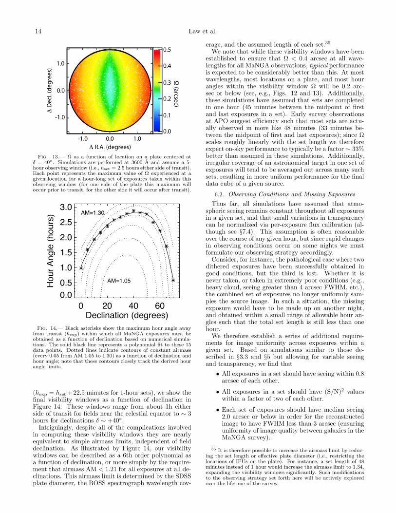
Fig. 15.— As Figure 5, but showing the impact of uncorrected bundle rotation on the reconstructed image quality. Note the markedincrease in FWHM and ellipticity of reconstructed point sources near the edges of the bundle for offsets ∼ 6.

We therefore simulate dithered observations of a con-stant surface-brightness source (e.g., like the outskirts ofa smooth elliptical galaxy), assuming typical observingconditions with visual seeing ∼ 1.5 arcsec. We mimicflux calibration errors by multiplying the fiber fluxes foreach exposure by a scale factor drawn randomly from agaussian distribution with a given RMS width and a me-dian of 1.0 before reconstructing the composite image.As illustrated in Figure 16, calibration errors betweenindividual exposures results in a stippling of the smoothbackground, introducing artificial spatial structure cor-related with the dithered fiber pattern.

In a single set of 3 exposures, we find that RMS fluxcalibration errors of 2% between exposures results in areconstructed image whose surface brightness varies by0.4% (RMS) from pixel to pixel. This is comparable tothe 0.3% pixel-to-pixel variations that we find in the re-constructed image assuming perfect flux calibration of

all exposures. As flux calibration accuracy degrades fur-ther to 5%, 15%, and 50% RMS between exposures, wefind pixel-to-pixel variations of 1%, 2%, and 8% respec-tively in the reconstructed image. If flux calibration er-rors are uncorrelated between exposures in different sets,this variation will average out over the course of obser-vations for a given plate. Even in the case where indi-vidual exposures are calibrated as poorly as to withina factor of 2, the pixel-to-pixel flux for a uniform back-ground source varies by just 2% RMS when averagedover 4 sets (12 total exposures). In contrast, preliminaryresults from MaNGA commissioning data indicate thatindividual exposures are typically calibrated to within2.5% (Yan et al. in prep), suggesting that flux calibra-tion errors are unlikely to contribute significantly to theimage reconstruction fidelity.

8. SUMMARY

MaNGA Observing Strategy 17

The MaNGA hardware design and observing strat-egy is driven by the desire to ensure high, uniform im-age quality and depth across all 10,000 of the galax-ies that will be observed during SDSS-IV. In particular,the goal of reaching 7% spectrophotometric accuracy be-tween [O II] λ3727 and Hα λ6564 requires that the recon-structed PSF varies by 10% or less (in both width andellipticity) across the face of each IFU. This goal is par-ticularly challenging given the variable total number ofexposures per field (∼ 6−20) required to reach the targetdepth, chromatic differential refraction arising from thelarge wavelength coverage of the survey (λλ3600−10, 000A), and field differential refraction caused by the 3 widefield of view over which individual IFUs are deployed.

We summarize the requirements necessary to meet ourgoal as follows:

1. Each IFU fiber bundle should be constructed of aregular hexagonal grid of fibers to an accuracy of5 µm rms. The MaNGA IFUs meet and exceedthis specification with a filling factor of 56% and atypical fiber placement accuracy of ∼ 3 µm rms.

2. Exposures should be obtained in sets of three 15-minute exposures dithered to the vertices of an1.′′44 equilateral triangle in order for each set touniformly sample the image plane.

3. The telescope must be able to dither to an accuracyof 0.′′1 or better.

4. Each plate should be observed for an integer num-ber of sets until the combined depth reaches asignal-to-noise ratio of 5 A−1 fiber−1 in the r-band continuum at a surface brightness of 23 ABarcsec−2.

5. All three exposures in a set must be observedwithin one hour of each other (i.e., the change inhour angle between the start of the first exposureand the end of the last exposure should be one houror less), and in a single plugging of a given plate.

6. All three exposures in a set should have (S/N)2within a factor of two of each other, and be ob-tained in atmospheric seeing that varies by lessthan 0.′′8. Each set should be obtained in medianseeing of 2.′′0 or better.

7. All MaNGA exposures should be obtained in vis-ibility windows ∼ 2 − 6 hours in length corre-sponding to airmass ≤ 1.21.

8. MaNGA relative flux calibration between expo-sures must be good to ∼ 5% or better.

In reality, many of the issues considered here will tendto average out over the course of the 3-4 sets that willtypically be obtained on a given plate since effects thatcause a slight gap in coverage for one set will often befilled in by another. However, our objective in designingthe MaNGA program is to ensure that the depth, cov-erage, and image quality of the entire survey is as goodand uniform as possible for the entire wavelength rangeof each of our 10,000 galaxies. In forthcoming contribu-tions (Law et al. in prep, Yan et al. in prep) we will

Fig. 16.— Simulated MaNGA observation of a constant surface-brightness field showing the characteristic stippling pattern intro-duced by relative flux calibration errors between dithered expo-sures. Such errors introduce artificial spatial structure correlatedwith the dithered fiber pattern. Greyscale stretch is arbitrary;in this example the blackpoint (whitepoint) is set to 20% below(above) the mean flux, corresponding to an RMS variation of about8% over the field of view. Note that the simulated field has beentrimmed to omit effects from regions at the edge of the IFU field.

explore in greater detail how well we succeed in meetingthese goals.

We thank Maryna Tsybulska for early contributions tothis project, and acknowledge the Summer Undergrad-uate Research Program at the Dunlap Institute, Uni-versity of Toronto for their support. AW acknowledgessupport of a Leverhulme Trust Early Career Fellowship.DRL thanks the anonymous referee whose comments ledto an improved version of the manuscript. Funding forthe Sloan Digital Sky Survey IV has been provided bythe Alfred P. Sloan Foundation and the Participating In-stitutions. SDSS-IV acknowledges support and resourcesfrom the Center for High-Performance Computing at theUniversity of Utah. The SDSS web site is www.sdss.org.

SDSS-IV is managed by the Astrophysical ResearchConsortium for the Participating Institutions of theSDSS Collaboration including the Carnegie Institutionfor Science, Carnegie Mellon University, the Chilean Par-ticipation Group, Harvard-Smithsonian Center for As-trophysics, Instituto de Astrofısica de Canarias, TheJohns Hopkins University, Kavli Institute for the Physicsand Mathematics of the Universe (IPMU) / Univer-sity of Tokyo, Lawrence Berkeley National Laboratory,Leibniz Institut fur Astrophysik Potsdam (AIP), Max-Planck-Institut fur Astrophysik (MPA Garching), Max-Planck-Institut fur Extraterrestrische Physik (MPE),Max-Planck-Institut fur Astronomie (MPIA Heidelberg),National Astronomical Observatory of China, New Mex-ico State University, New York University, The OhioState University, Pennsylvania State University, Shang-hai Astronomical Observatory, United Kingdom Par-ticipation Group, Universidad Nacional Autonoma deMexico, University of Arizona, University of ColoradoBoulder, University of Portsmouth, University of Utah,University of Washington, University of Wisconsin, Van-derbilt University, and Yale University.

18 Law et al.

REFERENCES

Bacon, R., Copin, Y., Monnet, G., et al. 2001, MNRAS, 326, 23Bacon, R., et al. 2010, SPIE, 7735Baldwin, J. A., Phillips, M. M., & Terlevich, R. 1981, PASP, 93, 5Belfiore, F., et al., 2015, MNRAS, 449, 867Bershady, Matthew A., Verheijen, Marc A. W., Westfall, Kyle B.,

Andersen, David R., Swaters, Rob A., Martinsson, Thomas 2010,ApJ, 716, 234

Bland-Hawthorn, J., Bryant, J., Robertson, G., et al. 2010,Proc. SPIE, 7735, 773541

Bolton, A. S., Schlegel, D. J., Aubourg, E., et al. 2012, AJ, 144,144

Bryant, J. J., Bland-Hawthorn, J., Fogarty, L. M. R., Lawrence,J. S., & Croom, S. M. 2014, MNRAS, 438, 869

Bundy, K., Bershady, M. A., Law, D. R., et al. 2015, ApJ, 798, 7Croom, S. M., Lawrence, J. S., Bland-Hawthorn, J., et al. 2012,

MNRAS, 421, 872Cuby, J. G., Bottini, D., & Picat, J. P. 1998, Proc. SPIE, 3355, 36Dawson, K. S., Schlegel, D. J., Ahn, C. P., et al. 2013, AJ, 145, 10Drory, N., et al., 2015, AJ, 149, 77Emsellem, E., Cappellari, M., Peletier, R. F. 2004, MNRAS, 352,

721Eisenhauer, F., Abuter, R., Bickert, K. et al. 2003, SPIE, 4841,

1548Fabricius, Maximilian H., Coccato, Lodovico, Bender, Ralf, Drory,

Niv, Gossl, Claus, Landriau, Martin, Saglia, Roberto P.,Thomas, Jens, Williams, Michael J. 2014, MNRAS, 441, 2212

Filippenko, A. V. 1982, PASP, 94, 715Gunn, J. E., Siegmund, W. A., Mannery, E. J., et al. 2006, AJ,

131, 2332Larkin, James E., Quirrenbach, Andreas, Krabbe, Alfred et al.

2003, SPIE, 4841, 1600Law, David R., Steidel, Charles C., Erb, Dawn K., Larkin, James

E., Pettini, Max, Shapley, Alice E., Wright, Shelley A. 2009, ApJ,697, 421

Li, C., et al., 2015, ApJ, in pressSanchez, S. F., Kennicutt, R. C., Gil de Paz, A., et al. 2012, A&A,

538, AA8Sharp, R., Allen, J. T., Fogarty, L. M. R., et al. 2015, MNRAS,

446, 1551Sharples, R., Bender, R., Berbel, A. et al. 2013, The Messenger,

151, 21Smee, S. A., Gunn, J. E., Uomoto, A., et al. 2013, AJ, 146, 32Weijmans, Anne-Marie, de Zeeuw, P. T., Emsellem, Eric, et al.

2014, MNRAS, 444, 3340Wilkinson, D.M., et al., 2015, MNRAS, 449, 328