Embed Size (px)
Citation preview

Occupancy Survey Guidelines
for Prairie Plant Species at Risk
Darcy C. Henderson
Prairie and Northern Region
Canadian Wildlife Service


OCCUPANCY SURVEY GUIDELINES FOR PRAIRIE PLANT SPECIES AT RISK Darcy C. Henderson1
August 2009 Canadian Wildlife Service Prairie and Northern Region 1 Prairie and Northern Wildlife Research Centre 115 Perimeter Road, Saskatoon, Saskatchewan CANADA S7N 0X4

Library and Archives Canada Cataloguing in Publication Henderson, Darcy C. (Darcy Christopher), 1970-
Occupancy survey guidelines for prairie plant species at risk / Darcy C. Henderson. Issued also in French under title: Lignes directrices du relevé d'occupation pour les espèces végétales en périls. Available also on the Internet. Issued by: Prairie and Northern Region. ISBN 978-1-100-15453-4 Cat. no.: En4-130/2010E
1. Vegetation surveys--Methodology. 2. Vegetation surveys--Prairie Provinces. 3. Rare plants--Sampling--Prairie Provinces--Methodology. 4. Endangered plants--Sampling--Prairie Provinces--Methodology. 5. Rare plants--Prairie Provinces. 6. Endangered plants--Prairie Provinces. I. Canadian Wildlife Service. Prairie and Northern Region II. Title. QH77 C3 H46 2010 333.95'321109712 C2010-980102-4 Cover photo credits: Western Spiderwort, © Candace Elchuk Slender Mouse-ear-cress, © Jennifer Neudorf Rough Agalinis, © Marjorie Hughes ©Her Majesty the Queen in Right of Canada, represented by the Minister of Environment, 2010
iii
SUMMARY Occupancy surveys fill a particular niche in generating information about the number of occurrences, area of occupancy and extent of occurrence of species. This data is needed to assess or rank the status of rare plants, and monitor the success of recovery actions for species at risk. These guidelines cover the most effective methods, expert tips and practical examples for surveying terrestrial grasslands to find new locations, or occurrences, of rare plant species. Rare plants do not lend themselves to the most well-known and widely available methods for sampling plant populations. These guidelines bring together a unique combination of scientific and technical information to help plan, execute or report on rare plant surveys. Individuals who undertake occupancy surveys and those who review and evaluate grant and permit applications for this work will also benefit from the information. Detectability, or the probability of finding a rare plant where it is known to occur, is one of the most important considerations for designing a rare plant survey. A properly prepared team is not the only ingredient for maximizing detectability, and other considerations, including survey timing, the year the survey takes place, search rate and sampling intensity will affect the outcome of a survey. These guidelines provide a checklist for maximizing detectability, and quantitative methods for estimating detectability. Occurrence locations are geographic data documented with attention to logistical, technical, biological and administrative considerations. Global positioning systems and geographic information systems have become essential tools for helping to integrate these requirements, and these guidelines outline how best to apply those tools. Survey layouts will depend on the size and complexity of the study area. Stratification will be necessary to make most efficient use of surveyor time and effective estimation of rare plant occurrence where multiple habitat types occur. Small study areas can be searched in their entirety, but larger study areas require some form of sampling. Sampling requires a lot of decision making about the best size and shape of a sample unit, the minimum sample size, and arrangement of sample units in the study area. These guidelines provide recommendations for all types of study areas and projects commonly encountered in the Prairie provinces. Data management and reporting are the final and lasting component of occupancy surveys. Future projects will benefit from well-documented survey designs and results, even if no plant occurrences were found. Absence-data documentation helps establish where a species does not occur, and eliminates question marks on the map. These guidelines outline how best to document and manage absence data, along with all other project data. Finally, there is consideration of what the minimum “data set” to report should be as an outcome to any and all occupancy surveys.


v
TABLE OF CONTENTS 1.0 ABOUT THESE GUIDELINES 1
1.1 Why are these guidelines needed?
1.2 Who needs these guidelines?
1.3 What is included and how are these guidelines organized?
1.4 When and where are occupancy surveys not enough?
1
1
2
2
2.0 FINDING RARE PLANTS – WHAT DOES IT TAKE? 3
2.1 Limitations of surveyors, plant dispersal and habitats
2.2 A seven-point checklist for maximizing detectability
2.3 Quantitative methods to estimate detectability
3
4
9
3.0 RECORDING AND DOCUMENTING RARE PLANT FINDS 10
3.1 Defining an occurrence
3.2 Filling grid cells
3.3 Marking transect segments
3.4 Mapping points and polygons
10
12
12
13
4.0 DESIGNING LAYOUTS FOR CENSUS-SURVEYS: SMALL STUDY AREA 16
4.1 Linear search patterns reduce bias
4.2 Census-survey of small patches <1 ha and narrow corridors <30 m wide
4.3 Stratified census-survey of landscapes <100 ha
16
16
17
4.3.1 Stratification versus bias
4.3.2 Minimum mapping unit scales for stratification
18
19
5.0 DESIGNING LAYOUTS FOR SAMPLE-SURVEYS: LARGE STUDY AREA 20
5.1 General principles of sampling 20
5.1.1 Representative stratified sample size threshold
5.1.2 Power and minimum sample size
20
21
5.2 Random or stratified sampling within buffer zones <300 m wide
5.3 Stratified random sampling of landscapes or regions
21
24
5.3.1 Landscapes lacking regular patterns
5.3.2 Regularly patterned landscapes
5.3.3 Valley and wetland complexes
24
25
26

vi
5.4 Phased or adaptive cluster-sampling landscapes 28
6.0 DOCUMENTING SEARCH-EFFORT AND ABSENCE DATA 29
6.1 Simple documentation
6.2 Automated GPS functions for documentation
29
29
7.0 MANAGING AND REPORTING PROJECT DATA 31
7.1 Data structure and relational tables
7.2 Minimum data set to report
31
32
8.0 ACKNOWLEDGEMENTS 34
9.0 REFERENCES 35
10.0 APPENDIX A: PLANT SPECIES AT RISK RESOURCES 38

1
1.0 ABOUT THESE GUIDELINES
1.1 WHY ARE THESE GUIDELINES NEEDED? Rare plants are restricted in distribution or abundance and often hard to find (McDonald 2004). Where rare plants have been afforded legal protection under the federal Species at Risk Act or similar provincial legislation, our primary objective is to find the specific locations where these plant species at risk occur in order to protect them and reduce liabilities of people who use or manage the habitat. Occupancy surveys are specifically designed to locate and describe these rare plant occurrences, and are often the optimal inventory strategy (Joseph et al. 2006). Occupancy survey techniques and methods for rare species are not well known or widely available, and commonly used sampling strategies to locate and map populations (see Elzinga et al. 2001) are not designed for the most rare and difficult to find species (Thompson 2004; MacKenzie and Royle 2005). Previous rare plant survey guidelines have focused on advice for small industrial sites in short-term projects, and for general natural history collections (see Bizecki-Robson 2000; Lancaster 2000; Wallis 2001; California Native Plant Society 2001). Different guidelines are needed to include complementary methods for the inventory of larger land parcels like parks and protected areas, military training areas, community pastures and grazing reserves, leased crown or public lands, and industrial buffer zones. These surveys may become the basis for changing land use or constraining development, so surveys need to be scientifically rigorous to justify the costs of subsequent actions (BC Ministry of Environment, Lands and Parks 1998; Fancy 2000; Thompson 2004; Kirk 2004; Vesely et al. 2006).
1.2 WHO NEEDS THESE GUIDELINES? Conservation science professionals will benefit most from these guidelines. In particular, people who regularly design, execute or report on rare plant surveys will identify with the familiar challenges presented, but may be surprised by some of the recommendations and methods used to overcome those challenges. Biologists with government agencies, environmental consultants and non-governmental land stewards are likely to be among those practitioners. People who evaluate rare plant survey designs or reports while reviewing environmental assessments, contract or grant proposals, species status reports, or other resource management plans will also find the content useful. In addition to biologists, this list may include academics, permit or contract specialists, enforcement officers, agronomists or other land managers. Plant species at risk in the Prairie provinces are also the focus of these guidelines (see list in Appendix A), so people working on these projects in Alberta, Saskatchewan, Manitoba, and the adjacent states of Montana and the Dakotas will find the guidelines most useful.

2
1.3 WHAT IS INCLUDED AND HOW ARE THESE GUIDELINES ORGANIZED? These guidelines include general concepts, literature references, specific examples, and quantitative or technical specifications for the design, execution and reporting components of occupancy surveys. General concepts often include definitions, and frequently used terms are highlighted in bold.
Flowcharts or bulleted and numbered lists describe concepts comprised of multiple components. Literature references are primarily refereed journal articles and scholarly books, with occasional
government or non-governmental organization publications where information cannot be found elsewhere.
Specific examples are drawn from Environment Canada projects, contractors and their reports, and
scientific literature relevant to temperate grasslands in the Prairie provinces. Figures and tables describing data are included where possible.
Quantitative or technical specifications are sometimes described as numbered lists of sequential
instructions, or priority options, and in some cases as equations or constants.
1.4 WHEN AND WHERE ARE OCCUPANCY SURVEYS NOT ENOUGH? It may make sense to put immediate investment in more detailed population enumeration and habitat description, rather than simple occupancy surveys:
Where there is considerable confidence a species is restricted to one or a few occurrences (i.e., island or locally endemic species); or
Where short-term demographic threats to the species outweigh long-term threats to habitat; or
Where an occurrence faces immediate extirpation due to human activity and any population or habitat information could be of conservation and mitigation value.
To learn more about the distribution and biology of rare plants in the Prairie provinces, there are several excellent reports and books (e.g., Argus and White 1978; Maher et al. 1979; White and Johnson 1980; Kershaw et al. 2001). Conservation Data Centres (CDCs) or Natural Heritage Information Centres (NHICs) also maintain databases of the most up-to-date rare plant occurrence records and status ranks in each province. The Species at Risk Public Registry has status reports and recovery strategies for all federally listed species (see Appendix A).

3
2.0 FINDING RARE PLANTS – WHAT DOES IT TAKE?
2.1 LIMITATIONS OF SURVEYORS, PLANT DISPERSAL AND HABITATS Personal characteristics of patience, perseverance and a positive attitude are essential for successfully completing rare plant surveys, because in many cases the result of a project will be no new occurrences after much effort at trying to find them. Aside from those personal characteristics, the overriding principle to keep in mind is that the purpose of the survey:
IS to objectively search available habitat for the target species, based on a pre-designed plan to reduce bias and increase accuracy and precision of estimates. Success should be measured by executing and confidently reporting the results of the survey regardless of whether the target species was found (MacKenzie and Royle 2005). IS NOT to subjectively hunt for the target species, based on natural history reasoning that cannot be repeated by another observer. Success should not be measured by simply finding a rare plant or finding one faster than anyone else."
Many rare species occurrence records have been a result of the latter process, or from incidental records in the course of monitoring vegetation. Most recorded rare plant occurrences are close to urban centres, access roads, or rights-of-way, only because people have spent more time searching these areas, and it is at these locations where threats to occurrences are most likely. This search and documentation bias is well known across North America (Moerman and Estabrook 2006), the data may not be useful for modeling critical habitat (Edwards et al. 2006), and threat information based on a few occurrences could lead to incorrect status assessments and inappropriate recovery plans by the Committee on the Status of Endangered Wildlife in Canada (COSEWIC). You cannot find rare plants everywhere, and part of the reason for their rarity may be a specialized habitat that is limited in space and time, or random long-distance dispersal events that create uncommon patchy distributions in a larger matrix of potentially suitable habitat. Many COSEWIC- listed plant species in the Prairie provinces do not occupy all available and suitable habitats within their extent of occurrence (EOO), which results in a smaller area of occupancy (AOO) than what is expected for common species with a similar EOO. Rare plant surveys do not always result in a rare plant find, in part because of these dispersal and habitat limitations, and also because of imperfect detectability during surveys. Detectability is the probability of finding a rare plant where it actually occurs (MacKenzie et al. 2002; Pollock et al. 2004), and is perhaps the most important consideration for rare plant surveys. In most cases you can never truly declare the absence of a species, because a number of factors may have reduced detectability. Thus it is more correct to refer to absence data as no-detection.

4
2.2 A SEVEN-POINT CHECKLIST FOR MAXIMIZING DETECTABILITY Many factors influence detectability, and it is a useful exercise to work through the following seven-point checklist for each and every rare plant survey. 1. Is the survey team organized, prepared and managed appropriately?
Target species characteristics should be studied from floras, herbarium specimens and photographs prior to a survey, and all similar species that could be mistaken for targets should receive similar attention. Independent evaluations of observer bias indicate many species, usually the rare ones, are regularly misidentified or overlooked in multi-species surveys of large plots (100 to 1000 m2) in temperate forests and grasslands (Archaux et al. 2006). Why these errors occur even amongst groups of experienced botanists appears to have a lot to do with how teams are organized and managed to keep people alert, motivated and equipped to cooperatively solve problems. Recommendations for an ideal team that will generate the most reliable data include having two or more individuals work together, one of whom possesses a decade or more experience in taxonomy of the local flora, and work days should start soon after sunrise and not exceed eight hours.
2. Is the habitat suitable for the target species?
We usually know very little about rare plant distribution and abundance, and we know relatively little about their habitat needs. For many rare grassland plants it is reasonable to assume a wetland or forest canopy does not provide suitable habitat, and for other species the texture and salinity of the soil may be key factors. Beyond these habitat characteristics that can be derived from soil survey maps and air
EXPERT TIP 1: To develop a search image for rare species that will extend the annual window of opportunity for surveys, begin a photo collection of accurately identified plants, under field conditions with vegetative individuals, seedlings and surrounding habitats, preferably from different locations and years. The Web is a great source for these photos if you do not have many of your own to start with.
photos, we cannot assume we “know” where these plants occur. For example, using long belt transects to sample all habitat types for two perennial plants anecdotally associated with sand dunes, Dalea villosa and Tradescantia occidentalis, resulted in the discovery that more plants occur in partly vegetated dunes and some are even found beneath a forest canopy (Godwin and Thorpe 2007). If only barren sand dunes were searched, much of the suitable habitat would remain unsearched, resulting in underestimated distribution and abundance, and inaccurate habitat, threat or management recommendations.
3. Is the time of year suitable for the target species?
Survey timing is usually organized to keep personnel busy and regularly employed over the snow-free season, however many rare native plants may only be detected for a few weeks each year. Phenological stages most readily detectable by observers should be used to plan targeted rare plant surveys (Table 2.1). While some evergreen perennials like soapweed yucca (Yucca glauca) can be observed nearly year-round, some annual and biennial plants

5
like slender mouse-ear-cress (Halimolobos virgata) can only be reliably identified for a few weeks in May and June during flowering and seed pod development. Multi-species surveys may require two, and rarely three, visits over the course of the snow-free season. To determine how many visits may be needed when planning a survey, consult regional floras and expert opinion.
BOX 1: Research shows…you are not as good as you think you are
The following points were derived from multiple sources, where researchers have specifically evaluated observer bias in monitoring programs for temperate forest or grassland species composition and cover in plots of varying size (see Klimes 2003; Kercher et al. 2003; Archaux et al. 2006; Vittoz and Guisan 2007; Johnson et al. 2008; Milberg et al. 2008; Archaux et al. 2009). The results may surprise you! Overlapping similarity of species lists collected by two or more experienced botanists in large-plot
multi-species surveys are on average 67% to 89% (range 45% to 98%), indicating botanists regularly misidentify or overlook species in the course of these surveys.
Misidentification rates in large-plot multi-species surveys are 5% to 10% for botanists with 10 to
30 years experience in the regional flora. Overlooking rates in large-plot multi-species surveys are >10% for botanists with experience in
the regional flora, and no time-limit restrictions. Overlooking and misidentification rates are greater for graminoids and bryophytes (difficult to
identify), while trees and shrubs (largest plants) are the least frequently overlooked or misidentified.
Overlooking rates increase as the area occupied by a species decreases, and below 1% cover the
overlooking rate increases exponentially from 10% up to 80%. Thus, it is more likely to miss a small rare species than a large common species.
Overlooking rates increase as the time spent searching decreases, such that <1 second m-2 will
normally detect only the most common species and sometimes >10 seconds m-2 are needed to detect the smaller and most rare species.
These results are from multi-species surveys, whereas surveys for a few specific rare species targets may involve more focus from a well-developed search image and corresponding lower rates of misidentification or overlooking. Nonetheless, people are fallible and results of rare plant surveys can never truly result in absences being confirmed. Thus, it is more correct to refer to presence-absence surveys as presence-no detection surveys.

6
Table 2.1 Interim recommended thresholds to maximize detectability of selected plant species at risk
Seasonal timing (months)
Transect width (m) Vegetation
Walk speed (km/hr) Vegetation
Species
Flowering Fruiting Tall-dense
Short-bare
Tall-dense
Short-bare
Slender mouse-ear-cress Lt May-Jun May-Jun 1 3 0.5 2 Western spiderwort Lt Jun-Jul Jul 2 5 1 3 Tiny cryptanthe Jun-Jul Jul-Sep 1 2 0.5 2 Small-flowered sand-verbena1
Jun-Aug Jul-Aug n/a 3 1 3
Buffalograss2 Lt Jun-Jul Jul-Sep 1 4 1 3 Hairy prairie-clover Jul-Aug Aug-Sep 2 6 1 4 Soapweed (Yucca) Jun-Jul Year-round 5 10 3 5 1 Seedlings are distinctive and can be readily detected on the barren sand habitat beginning early May. 2 Stolons connecting ramets are distinctive if observed in close proximity and can be seen year-round. 4. Is the year suitable for the target species?
Fluctuations in abundance can occur in response to climate, and this affects whether a rare species will be detected even if it is present as seeds or dormant buds in the soil. Dry and cold spring conditions can cause lady’s slipper (Cypripedium) buds to remain dormant on creeping rootstocks, resulting in underestimates of abundance (Kery 2004). To determine suitability of the year, first consult local and regional climate patterns for the past week, growing season to date, or a longer interval that may be most relevant to the target species under consideration. Second, revisit one or more previously known locations to compare present density and detectability with that documented in the past.
5. Is the search width suitable? 6. Is the search speed suitable?
Both the speed of travel and search width combine to affect the search rate, and what is an appropriate rate will vary with the above factors as well as plant size and obstructing vegetation cover (Figure 2.1). In large plots used to describe species richness, the largest plants or most common species with cover >1% are normally detected in the first few minutes, while rare species make up the bulk of plants found in the minutes or even hours thereafter. Unlike misidentification error rates, the rate of overlooking species in multi-species inventories range from 10% to 30% when searching at an equivalent rate
EXPERT TIP 2: Plan multi-species surveys to target the most difficult-to-detect species, and plan for search rates and seasonal timing that best suits those problem species.
of 9 seconds m-2 (Archaux et al. 2009). Targeted searches for one or a few rare species should improve on that overlooking rate. However, in controlled detectability trials conducted by Environment Canada using pipe cleaners fashioned to resemble tiny cryptanthe, observers with varying levels of experience only found an average 70% of the individuals placed in a mowed lawn at search rates of 3 to 8 seconds m-2. When in doubt, consult expert opinion or conduct detection trials to determine the appropriate search rate.

7
Figure 2.1 Variability in time to complete a search within 500 x 5 meter belt transects for various habitats and target species: (dashed line) buffalograss on flat mixed-prairie in SE Saskatchewan, mean = 14.6 min; (solid line) hairy prairie-clover on partly wooded rolling sand dunes in SW Manitoba, mean = 19.6 min; (dotted line) tiny cryptanthe on undulating to rolling dry mixed-prairie in SE Alberta, mean = 24 min (data source: Environment Canada). 7. Is there sufficient sampling intensity?
Small study areas can be census-searched, but larger study areas may only be sampled. Determining the proportion of the study area to search, and in what arrangement of sample units, is the major subject of Section 5. Unlike most vegetation sampling methods, rare plant surveys need to cover much more ground but with the focused attention to the target species. Large plots and long belt transects with >500 m2 are usually necessary to detect rare plants, unlike quadrats <1 m2 or pin frames used to sample the abundance of the most common plant species (Stohlgren 2006). The more plots or transects used will increase the proportion of the study area sampled and will increase detection probability of the target (Figure 2.2).
8
0
20
40
60
80
100
0 5 10 15 20 25
Transect Density
Det
ecta
bilit
y (%
)
2004
2005
2006
2007
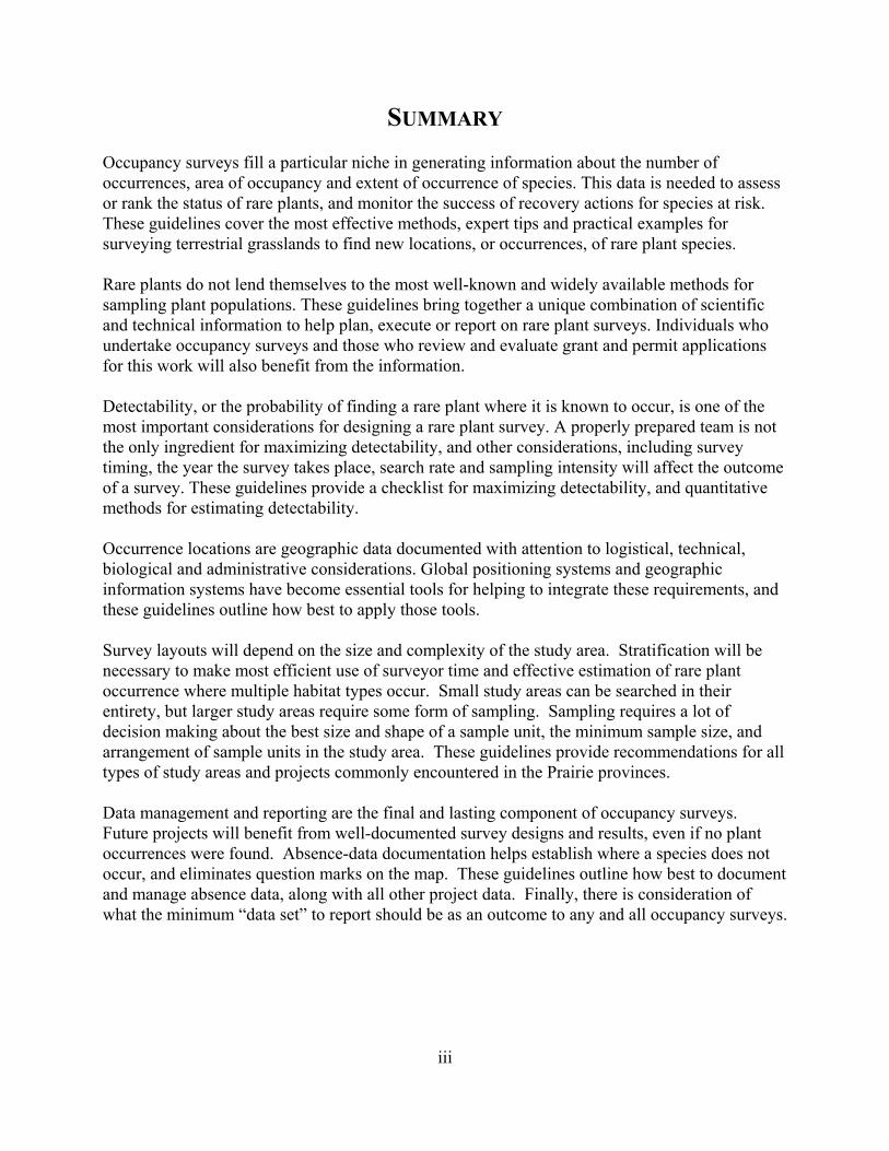
Figure 2.3 Detectability as a function of sampling intensity for slender mouse-ear-cress at Prairie National Wildlife Area #20. Following census-surveys, the known area of occupancy was mapped each year from 2004–2007. Simulated sampling was conducted with randomly located 800 x 2 metre belt transects overlaid on the 800 x 800 metre quarter section to estimate detectability. Results are a count of hits after 100 iterations of each transect density level (data source: Environment Canada).
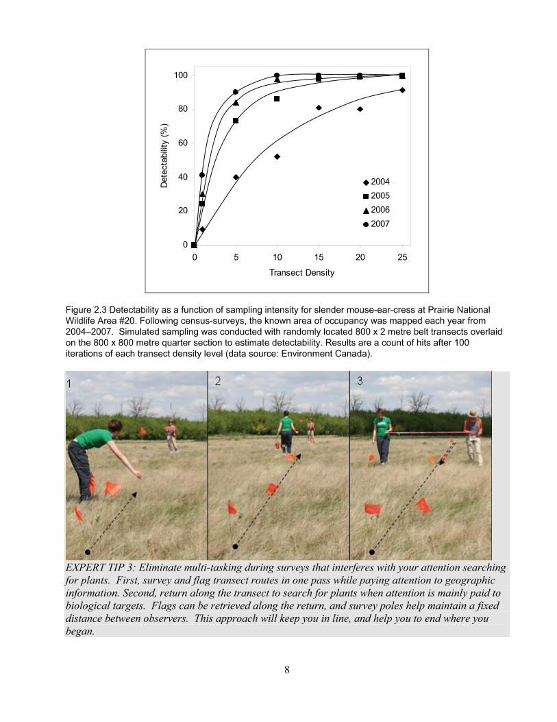
EXPERT TIP 3: Eliminate multi-tasking during surveys that interferes with your attention searching for plants. First, survey and flag transect routes in one pass while paying attention to geographic information. Second, return along the transect to search for plants when attention is mainly paid to biological targets. Flags can be retrieved along the return, and survey poles help maintain a fixed distance between observers. This approach will keep you in line, and help you to end where you began.

9
2.3 QUANTITATIVE METHODS TO ESTIMATE DETECTABILITY For an added sense of credibility a rare plant survey should quantitatively estimate detectability. Double sampling by different observers, at different times, using the same sampling protocol.
Some occurrences found by one observer will be overlooked by another observer, and vice versa. The number of occurrences recorded by both divided by the total number of all occurrences will equal a detection probability usually <1. This is identical to the method used for estimating similarity indices in community ecology. Replicated double sampling can also be used to generate a more accurate detection probability average with a measure of variation.
D = (2 * c) / (a + b)
a = occurrences or individuals recorded by observer 1 b = occurrences or individuals recorded by observer 2 c = occurrences or individuals recorded and in common to both observers D = detection probability
Double sampling by different observers using different sampling protocols. Option 1 (double
observer) involves the first observer marking all occurrences he or she find while simultaneously the second observer records the first observer’s finds, and adds the second observer’s own additional occurrences. Option 2 is to have the first observer use a standard but rapid sampling protocol while the second observer uses an extremely intensive protocol to document all overlooked occurrences possible. In both cases the number of occurrences recorded by the first observer is divided by those of the second observer to equal a detection probability usually <1. Replication is also advised for this approach to estimate average and variance.
D = a / b
a = occurrences or individuals recorded by observer 1 b = occurrences or individuals recorded by observer 2 D = detection probability
Detection probabilities >1 sometimes result from misidentification and inclusion of the wrong species or exclusion of the right species, or by incorrectly including or excluding individuals that occur on or near the edge of sample units, or mistakenly double-counting a single occurrence or individual. These errors
EXPERT TIP 4: Replicated detection trials should represent all observers, habitats, target species and search rates. If lots of variation occurs, the average may not be as meaningful as examining separately the different detection probabilities under each set of conditions
of commission will occur and have occurred in experimental trials, which further emphasize the need for replication of detectability trials to best estimate these probabilities. Ultimately, detection probabilities can be used to correct estimates of distribution and abundance (see detailed calculations in MacKenzie et al. 2002; Pollock et al. 2004; Rondinini et al. 2006). Essentially the true number of occurrences or individuals (N) is equal to those counted (C) divided by the detection probability (P).
N = C / P

10
3.0 RECORDING AND DOCUMENTING RARE PLANT FINDS Historically it was physical collections of plants, usually pressed and preserved for a public or private herbarium that constituted evidence of a plant find. However, there are now many technological means to increase the accurate and precise geographic information needed for planning mitigations or recovery and monitoring programs for rare plants, and to leave the plants in-situ. All of those methods depend on a clear definition of what constitutes an occurrence.
3.1 DEFINING AN OCCURRENCE An occurrence is one or more plants of a single species that share a point, line or polygon in space. Factors affecting the definition of an occurrence for a particular field-based survey may include the following:
1. Logistically, an occurrence will depend on the desired resolution of the project. Where presence or absence at the quarter-section scale is desired in a landscape or regional project, any physical evidence of the species in that area constitutes an occurrence and is recorded as present for the quarter-section. The same can be done for habitat patches defined at landscape to site scales. However, more resolution is usually desired.
2. Technically, the minimum mapping units for NatureServe Biotics is 12.5 metres (U.S.A.) or
25 metres (Canada) based on the use of either 1:25 000 or 1:50 000 map scales (NatureServe 2004). More precision is always possible in the field, and most hand-held Global Positioning Systems (GPS) available by 2010 have a positional accuracy of less than ± 5 metres. Surveyor total stations can achieve accuracy to within millimetres.
3. Biologically, not all plant parts can be observed aboveground (i.e., lateral roots or soil
seedbanks), many plants reproduce vegetatively and not all single stems are genetically distinct individuals (genets) but rather clones of a single parent (ramets), and many plants have a small basal area relative to the diameter or coverage provided by the canopy. Therefore, species-specific decisions must be made to group, split or buffer what can be observed aboveground by surveyors into biologically meaningful occurrences (Table 3.1).
4. Administratively, organizations may use standard definitions applied to all plant species after
a survey. NatureServe and member CDCs or NHICs classify occurrence records into element occurrences (EO) that may group or split polygons or clusters of points on the basis of distance, habitat connectivity or similarity (NatureServe 2004). Similarly, COSEWIC estimates area of occupancy on the basis of 1x1 km and 2x2 km UTM grid squares, regardless of whether a record occupies all or a small portion of each grid square.

11
BOX 2: Should you collect voucher specimens of plant species at risk? Collecting whole plants, plant parts or seeds of a plant species at risk may represent a threat to survival and recovery of some populations. Voucher specimen collection to facilitate detailed taxonomic identification and provide physical evidence of occurrence is a prohibition under sections 32 and 36 of the Species at Risk Act (Government of Canada 2002). However, with the appropriate permits it is possible to collect a plant or plant part for the purposes of confirming taxonomy. Collecting and preserving a plant requires care to ensure structures essential for accurate identification are not damaged (see Alberta Native Plant Council 2006 for more information on plant collection, pressing and preservation). The question remains, how many plants can be safely collected. Menges et al. (2004) conducted population viability analyses and estimated extinction risks for a range of perennial plant species under various scenarios of initial population size, seed collection extent and frequency. Based on that analysis, Menges et al. (2004) recommended that less than 10% of the seed produced by a population in a given year be collected once every 10 years, regardless of population size, to ensure a 95% probability of population persistence. We could extend this to mean only 1 in 10 individuals should be collected as voucher specimens from a given population, once every 10 years; but it is difficult to extrapolate the impact of seed collection to the collection of whole plants. Digital photography in-situ is preferred for plant species at risk, instead of voucher specimen collections. Advantages of digital cameras: In common-use and readily available, more so than plant presses; Provide extremely high resolution images equivalent to dissecting microscope quality; Photo quality can be reviewed immediately to ensure high quality images are taken from a living
specimen, while damage to a plant during collection cannot be undone; Memory limitations on the number of images and specimens photographed are minor, compared
with space limitations for pressed specimens; Images can be archived permanently with little or no degradation, while pressed specimens can be
damaged, desiccated, and lose colour over time such that the most important identifying structures are difficult to observe;
Habitats can also be photographed for independent classification of the habitat type, which is often more informative than the single and subjective narrative description;
Perhaps the greatest advantage of digital photographs is the ease with which images can be circulated to multiple plant taxonomy experts in multiple locations for confirmation of identification, while pressed specimens usually cannot be removed from the herbarium where they are stored.
Disadvantages of digital cameras include: Scale is missing from photographs, and size of structures is often important for identification; Important structures needed for identification may have been overlooked. Precise location
coordinates taken with GPS can facilitate relocation for more photographs with a scale bar.

12
Table 3.1 Changing definitions of what constitutes an individual plant species at risk based upon the life form, life history, and perspective or objective of the definition
Species Evolutionarily relevant unit for selection
COSEWIC status assessment unit
Practical and efficient unit to observe in the field
Sand-verbena Slender mouse-ear-cress Hairy prairie-clover Soapweed Buffalograss Alkaline wing-nerved moss
Seed and plant Seed and plant Genet Genet Genet Spores
Shoot & flower or fruit Shoot & flower or fruit Ramet or single shoot Ramet or single shoot Ramet or single shoot Patches
Rooted shoot Flowering shoot (not rosettes) Rooted shoot Rosette Patch or foliar cover Patches with sporophytes
3.2 FILLING GRID CELLS Grids may be specific to a survey plan to capture a predefined resolution of data, or one of the existing geographic or land survey grids can be used instead.
1. Dominion Land Survey grids divide most of Western Canada into 10x10 km townships, each of which is comprised of 36 sections each 1.6x1.6 km, each of which can be subdivided into four quarter sections 0.8x0.8 km or into 16 legal subdivisions 0.4x0.4 km in size. This approach has been used in census-surveys for buffalograss in southeastern Saskatchewan to specifically increase our knowledge of the EOO and AOO at the quarter-section scale.
2. Universal Transverse Mercator Grid divides the planet into a metric network of squares that
are most often represented at the 1x1 km resolution on maps with 1:50 000 or 1:250 000 resolution. Below a grid resolution of 100x100 m the risk of accuracy errors increases in the UTM grid or the occurrence data.
3.3 MARKING TRANSECT SEGMENTS Belt transects pre-designed to have geographically identified start and end points, and fixed widths, are ideal for sampling occurrences and sometimes for estimating population size. Depending upon the size of the occurrence in relation to the belt transect, there are two basic ways to identify the occurrence.
1. Single plants or patches of plants much smaller than the width of a belt transect may be identified by specific points with a pair of both E-W and N-S coordinates. But assuming the likelihood of a zone of influence surrounding the plant that contains living roots and a soil seedbank, it may be wise to define these small occurrences as segments of the larger transect.
2. Patches of one or more plants larger than the width of a belt transect are readily identified
by starting and ending coordinates of a transect segment, and an area of occupancy is

13
automatically generated by multiplying the segment length by the fixed width of the belt transect. This approach has been used to monitor tiny cryptanthe populations in the Suffield National Wildlife Area, and to estimate population size of hairy prairie clover in the Dundurn sandhills.
EXPERT TIP 5: Transects oriented on a constant latitude, longitude, easting or northing make it easy to mark occupied segments, because start or end points only require recording a single number. This saves time and reduces error in hand transcription, or simplifies digital input.
Segments do not always represent discrete patches and may simply be several lobes of a larger single patch occurring next to a belt transect. That is not always a concern for the belt transect method, where calculations and monitoring to detect change occurs with phenomena that are measured within the transect only. Figure 3.1 Conceptual representation of how transect segments are used to identify occurrences in long belt transect surveys. This example is of a transect on a constant UTM easting, so only northings are recorded to describe the segments.
3.4 MAPPING POINTS AND POLYGONS The “Track” function available on most GPS units is the most efficient means to mark points and polygon boundaries of rare plant occurrences. Tracks simply record a sequence of points on a time (5 seconds to several minutes) or distance (5 metres or more) delay, and this function can be turned on and off to reduce the memory requirement. Decisions need to be made about the maximum distance between plants in order to be mapped as the same polygon, and hopefully this is decided upon when defining an occurrence for the purposes of your project. Where the objective is to apply buffers for avoidance constraints on an industrial development, plants that are closer together than double the buffer distance can be grouped. Conversely, where the information is intended for multiple users for multiple purposes, mapping should be as precise as that allowed by the equipment, and polygons as small as 2x2 metres can be created.
Occurrence 1
N 5556789
Occurrence 2Start N 5556775End N 5556765
Occur
renc
e 3
N 555
6759
Occurrence 4Start N 5556699End N 5556694
2 m widetransect
Occurrence 1
N 5556789
Occurrence 2Start N 5556775End N 5556765
Occur
renc
e 3
N 555
6759
Occurrence 4Start N 5556699End N 5556694
Occurrence 1
N 5556789
Occurrence 2Start N 5556775End N 5556765
Occur
renc
e 3
N 555
6759
Occurrence 4Start N 5556699End N 5556694
2 m widetransect

14
0 0.5 10.25 Kms 0 100 20050 m
2004
2005
2006
2007
Figure 3.2 Polygons created with GPS will appear more or less detailed depending upon the resolution desired. Image at left describes hairy prairie-clover patches where plants <30 m apart were grouped into polygons. Image at right describes slender mouse-ear-cress patches in multiple years where plants <2 m apart were grouped into polygons.
EXPERT TIP 6: Before using a GPS to map the perimeter of a polygon, first mark the perimeter with temporary pin flags through a careful systematic search for the plants without a GPS. Afterwards, you can then focus attention on the GPS to monitor satellite reception, position accuracy and ensure the track is recording properly while you remove flags on the second pass. The resulting data can be downloaded as a sequence of points, and projected in a low-tech (MS Excel chart) or high-tech (GIS geospatial data layer) environment. GPS specifications recommended include:
1. Using a 5 to 10 second delay increment while walking 2 to 4 km/hour. Longer time delays or a distance function >10 m result in less accurate representations with frequent cross-over or gap errors where you start and end mapping the polygon lines.
15
2. Recording tracks only after the location error has stabilized at or below 5 metres to minimize
those same cross-overs or gap errors that occur when reception changes among multiple satellites. These errors are expected but within reason for accurate locations.
Alternative approaches to measuring occurrences and calculating the area of occupancy do exist but should be avoided where possible for the following reasons.
1. Waypoints along polygon boundaries consume more time and memory, and limit what you can accomplish in a survey (i.e., Garmin E-trex Vista 2006 can only store 250 waypoints, but up to 10 000 track points).
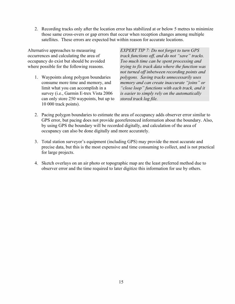
EXPERT TIP 7: Do not forget to turn GPS track functions off, and do not “save” tracks. Too much time can be spent processing and trying to fix track data where the function was not turned off inbetween recording points and polygons. Saving tracks unnecessarily uses memory and can create inaccurate “joins” or “close loop” functions with each track, and it is easier to simply rely on the automatically stored track log file.
2. Pacing polygon boundaries to estimate the area of occupancy adds observer error similar to GPS error, but pacing does not provide georeferenced information about the boundary. Also, by using GPS the boundary will be recorded digitally, and calculation of the area of occupancy can also be done digitally and more accurately.
3. Total station surveyor’s equipment (including GPS) may provide the most accurate and
precise data, but this is the most expensive and time consuming to collect, and is not practical for large projects.
4. Sketch overlays on an air photo or topographic map are the least preferred method due to
observer error and the time required to later digitize this information for use by others.

16
4.0 DESIGNING LAYOUTS FOR CENSUS-SURVEYS: SMALL STUDY AREA 4.1 LINEAR SEARCH PATTERNS REDUCE BIAS Intersecting or overlapping survey transects or plots could result in the repeated measurement of the same individual or patch, which inflates estimates of density by including errors of commission. This would include “meandering” or “random walk” search patterns that are sometimes advocated (Figure 4.1). This is an unrepeatable method that does not allow an objective calculation of search effort, because meanders vary in frequency and amplitude leading to both random and systematic errors in accuracy that cannot be corrected (Edwards et al. 2006). This is why linear, parallel and adjacent transects are recommended in nearly all cases to reduce those sources of bias that lead to low detectability and low quality of survey results.
EXPERT TIP 8: To keep on track with parallel and adjacent transects, use temporary pin flags to mark the outside boundary of a belt transect while searching, then swing around and retrieve these flags on the next pass while searching. The lines do not have to be perfectly straight, but it helps ensure you do not miss anything like you would with meanders.
Figure 4.1 Conceptual representation of random and systematic cross-over and gap errors created by the uncontrolled frequency and amplitude of “meanders” relative to parallel and adjacent linear transects.
17
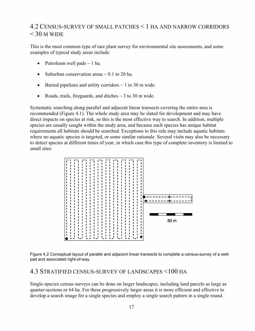
4.2 CENSUS-SURVEY OF SMALL PATCHES < 1 HA AND NARROW CORRIDORS < 30 M WIDE This is the most common type of rare plant survey for environmental site assessments, and some examples of typical study areas include:
Petroleum well pads ~ 1 ha.
Suburban conservation areas ~ 0.1 to 20 ha.
Buried pipelines and utility corridors ~ 1 to 30 m wide.
Roads, trails, fireguards, and ditches ~ 3 to 30 m wide. Systematic searching along parallel and adjacent linear transects covering the entire area is recommended (Figure 4.1). The whole study area may be slated for development and may have direct impacts on species at risk, so this is the most effective way to search. In addition, multiple species are usually sought within the study area, and because each species has unique habitat requirements all habitats should be searched. Exceptions to this rule may include aquatic habitats where no aquatic species is targeted, or some similar rationale. Several visits may also be necessary to detect species at different times of year, in which case this type of complete inventory is limited to small sites. Figure 4.2 Conceptual layout of parallel and adjacent linear transects to complete a census-survey of a well-pad and associated right-of-way.
4.3 STRATIFIED CENSUS-SURVEY OF LANDSCAPES <100 HA Single-species census surveys can be done on larger landscapes, including land parcels as large as quarter-sections or 64 ha. For these progressively larger areas it is more efficient and effective to develop a search image for a single species and employ a single search pattern in a single round.
50 m50 m

18
Search times for study areas as large as a quarter section could vary from a low of 40 to a high of over 100 person-hours, assuming the species is absent or not detected. Systematic searching along parallel and adjacent linear transects covering the entire area is recommended. Normally the whole area is not immediately threatened by development, and the survey can be completed progressively over the course of days if necessary. For efficiency, some clearly unsuitable habitats could be excluded from searching through division of a more heterogeneous or variable study area into many smaller habitat units that are more similar or homogenous at that smaller scale (Figure 4.2). This is called stratification. 4.3.1 STRATIFICATION VERSUS BIAS Stratification contrasts with bias in several important ways:
Stratification is a conscious, preplanned effort to exclude, reduce or increase search intensity among patches that differ in some measured and repeatedly observed habitat characteristic. Stratification then allows quantitative estimation of varying search intensity, quantitative evaluation of how that affected results, and correctly limits or weights extrapolation of results among habitat patches.
Bias is a term usually reserved for unplanned, conscious or subconscious, decisions made
on-site to adjust search intensity. Bias results in variability caused by observer error that cannot be quantified, repeated or extrapolated.
Figure 4.3 Conceptual layout of parallel and adjacent linear transects to complete a stratified census-survey of grassland habitats in a quarter-section.
Tree & Shrub Cover
Grassland
Grassland (sand)
Wetland
500 m
Tree & Shrub Cover
Grassland
Grassland (sand)
Wetland
Tree & Shrub Cover
Grassland
Grassland (sand)
Wetland
500 m

19
4.3.2 MINIMUM MAPPING UNIT SCALES FOR STRATIFICATION Stratification of habitats in the Prairie Ecozone can be simple or difficult depending upon the complexity and scale.
1. Simple, coarse-scale and repeatable stratification is recommended, because the habitats of rare plant species are not always well known. For example, tiny cryptanthe and slender mouse-ear cress both occupy dry coarse-textured soils within mixed-grass prairie, in which case all grassland on coarse soils that are not wetlands or forests represent potential habitat. Minimum mapping units of 1 to 0.25 ha are suggested.
2. Moderately complex, medium-scale stratification that separates habitats based on a few
simple criteria is an ideal case. For example, alkaline wing-nerved moss will only occur in margins of alkaline wetlands, and hairy prairie clover will only occur on coarse-textured soils on or adjacent to sand dunes with little or no shrub canopy cover. Minimum mapping units of 0.25 to 0.01 ha are suggested.
3. Complicated, fine-scale strata that separate patches based on dominant plant species or
species assemblages, despite similar vegetation structure, soil type, and climate are difficult to separate in advance of a survey, and difficult to justify unless detailed and species-specific competitive or other functional effects are well understood. Although species lists are commonly recorded for rare plant occurrences, this data is rarely useful for the above reason. Stratification <0.01 ha is not recommended for occupancy surveys.

20
5.0 DESIGNING LAYOUTS FOR SAMPLE-SURVEYS: LARGE STUDY AREA
5.1 GENERAL PRINCIPLES OF SAMPLING Where larger areas of land are to be surveyed, census techniques become less practical and a sampling plan must be employed to estimate the number of occurrences and area of occupancy. Three principles of sampling habitats that help reduce biased estimates include:
1. Randomization of sample units. Randomization of sample unit locations can be achieved by selecting numbers from a random number table, generating random numbers digitally or using random location functions in a Geographic Information System (GIS).
2. Independence of sample units. Independent units are usually equal in area and shape, do not
overlap, and are sampled at the same time to the extent possible. Linear belt transects should always be parallel to avoid the likelihood of cross-overs or intersections, and all types of sample plots should avoid sharing boundaries where overlap is most likely.
3. Replication of sample units. Replication allows estimation of variability and central
tendency in the data. The minimum number of replicates required will be affected by the time and resources available, the size of sample units selected, and some predetermined mathematical criteria for minimum acceptable errors.
To determine the minimum sample size needed, there are two general means that employ inferential statistics. Consult a statistics text for equations and software recommendations. 5.1.1 REPRESENTATIVE STRATIFIED SAMPLE SIZE THRESHOLD Often you simply want to know if you have replicated random sample units enough to represent the proportional distributions of habitats in the study area, and you want to do this in advance of a survey with only map-based information to go on (MacKenzie and Royle 2005). This is particularly true of an area where no surveys have occurred before, and no biological information about habitat preferences of the target species are available.
1. First, create an expected distribution based on the proportional distribution of all stratified and potentially sampled habitats in the study area.
2. Second, create one or more observed distributions based on the proportional distribution of
all habitat strata contained in one or more random samples of survey units. Assuming a detection probability >50% you need to have at least two survey units in your sample.
3. Third, use an iterative goodness of fit or chi-squared test to determine at what point a
progressively larger observed sample size creates an observed distribution that is no longer different from the expected distribution of habitats. Depending upon how many strata you

21
create or the size of survey units, the type 1 error rate can be set between 10% and 1% (α = 0.1 to 0.01), and the statistical test only works for sample sizes >4 survey units.
This process can be automated in GIS applications given a sample unit of known size and shape. If you are still failing to sample the most-rare habitats, you can purposely select those habitats to improve representation. A minimum number of samples per stratum can be selected in GIS applications to improve representation while minimizing bias. 5.1.2 POWER AND MINIMUM SAMPLE SIZE If your objective is to specifically estimate population size, occurrence density or area of occupancy for a rare plant species, then you need some information from past studies and you have to decide upon some specific criteria.
1. Find or estimate variance for a given sample size based on previous studies or professional
expertise. This is often the most difficult information to gather or estimate for a rare species about which we know very little.
2. Pre-select acceptable thresholds for precision of estimates. Statistical confidence limits
should not overlap zero, so the sample variation must be low; if possible, no sample units should have zero values, and detection probability may be used to drag confidence limits away from zero. Often a maximum type 1 error rate of 10% or α = 0.1 is desired.
3. Pre-select acceptable thresholds for detecting trends or differences over time or between
habitats. This effect size needs to be greater than error caused by uncontrolled observer bias (misidentification, overlooking, commission errors) and environmental variation. Often a minimum effect size threshold of 20% to 40% may be reasonable.
4. Pre-select acceptable thresholds for type 2 error rate and thus the power of the test (1 –
type 2 error). Power is the probability that a difference truly does exist and your data was sufficient to detect the difference. In the case of rare species where the risks of not detecting a declining or increasing trend may be high from biological, legal and economic standpoints, power should also be high (>70%). Retrospective power analysis based on information in 1 to 3 above will estimate actual power achieved, or by selecting the desired power a priori you can estimate the minimum sample size needed.
Generally, power increases with an increase in sample size, effect size or type 1 error rate, and a decrease in variance. Consult a statistics text or software package for more information.
5.2 STRATIFIED OR RANDOM SAMPLING WITHIN BUFFER ZONES <300 M WIDE Systematic searching along parallel and adjacent linear transects covering the entire development area is recommended (see Section 4.2). However, there are cases where additional sampling in buffer zones may be required where a set-back distance buffer is placed around the development

22
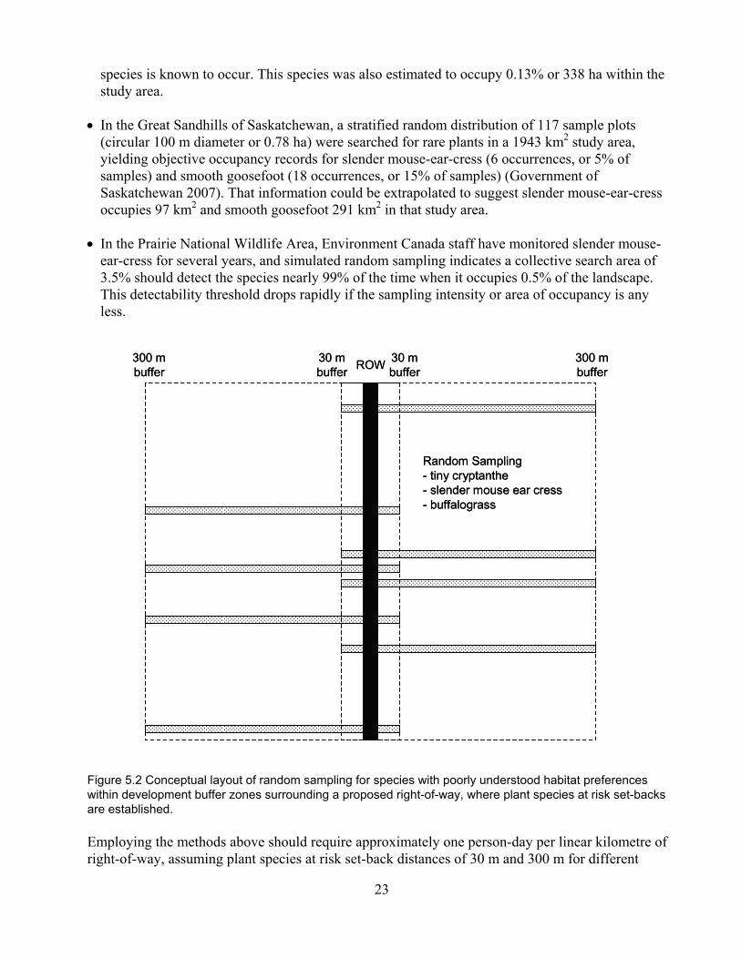
area. The combined effort of both census-search in the development zone and sampling in the buffer should be aimed at maximizing detectability through adequate sampling intensity. For species with well-known habitat affinities, a reasonable sampling intensity would depend on the distribution of those habitats and whether the study area is within the known EOO (Figure 5.1). For example, within dune sand polygons from soil surveys of the Prairie Ecozone, an average of 3% to 5% of the landscape is barren or sparsely vegetated dunes (Environment Canada unpublished analyses), and these are the preferred habitats of several plant species at risk. Figure 5.1 Conceptual layout of stratified sampling for species with well-known habitat preferences within development buffer zones surrounding a proposed right-of-way, within plant species at risk set-backs. For species with unknown or poorly understood habitat affinities, some minimum stratification and sampling threshold is warranted. Random sampling of 3% to 5% of the landscape should detect species that occupy as little as 0.2% to 0.3% of the sample area. For upland grassland species, it may be most efficient to stratify and exclude wetlands and forests from consideration, and then randomly sample the remaining grassland (Figure 5.2). Some examples of where this random sampling has worked include: In the Suffield National Wildlife Area, Environment Canada staff have detected tiny cryptanthe
along 1 of every 15 random belt transects (500x2 m) within a 260 km2 study area where the
ROW30 mbuffer
30 mbuffer
300 mbuffer
300 mbuffer
Sand Dune Stratum- small-flowered sand verbena- western spiderwort- hairy prairie clover- smooth goosefoot
Wetland Margin Stratum- alkaline wing-nerved moss- dwarf woolyheads- western blue flag
ROW30 mbuffer
30 mbuffer
300 mbuffer
300 mbuffer
Sand Dune Stratum- small-flowered sand verbena- western spiderwort- hairy prairie clover- smooth goosefoot
Wetland Margin Stratum- alkaline wing-nerved moss- dwarf woolyheads- western blue flag
23
species is known to occur. This species was also estimated to occupy 0.13% or 338 ha within the study area.
In the Great Sandhills of Saskatchewan, a stratified random distribution of 117 sample plots
(circular 100 m diameter or 0.78 ha) were searched for rare plants in a 1943 km2 study area, yielding objective occupancy records for slender mouse-ear-cress (6 occurrences, or 5% of samples) and smooth goosefoot (18 occurrences, or 15% of samples) (Government of Saskatchewan 2007). That information could be extrapolated to suggest slender mouse-ear-cress occupies 97 km2 and smooth goosefoot 291 km2 in that study area.
In the Prairie National Wildlife Area, Environment Canada staff have monitored slender mouse-
ear-cress for several years, and simulated random sampling indicates a collective search area of 3.5% should detect the species nearly 99% of the time when it occupies 0.5% of the landscape. This detectability threshold drops rapidly if the sampling intensity or area of occupancy is any less.
Figure 5.2 Conceptual layout of random sampling for species with poorly understood habitat preferences within development buffer zones surrounding a proposed right-of-way, where plant species at risk set-backs are established. Employing the methods above should require approximately one person-day per linear kilometre of right-of-way, assuming plant species at risk set-back distances of 30 m and 300 m for different
ROW30 mbuffer
30 mbuffer
300 mbuffer
300 mbuffer
Random Sampling- tiny cryptanthe- slender mouse ear cress- buffalograss
ROW30 mbuffer
30 mbuffer
300 mbuffer
300 mbuffer
Random Sampling- tiny cryptanthe- slender mouse ear cress- buffalograss
24
developments. Where more than one species is expected, and phenological patterns also differ such that a single visit is unlikely to detect both species, then two visits are required. The most time-sensitive species to detect is slender mouse-ear-cress (28 days from mid-May to mid-June) and western spiderwort (28 days in the month of July), in which case 28 linear km would be the maximum searchable area per person, per year. Accessibility and labour availability could further limit the distance covered.
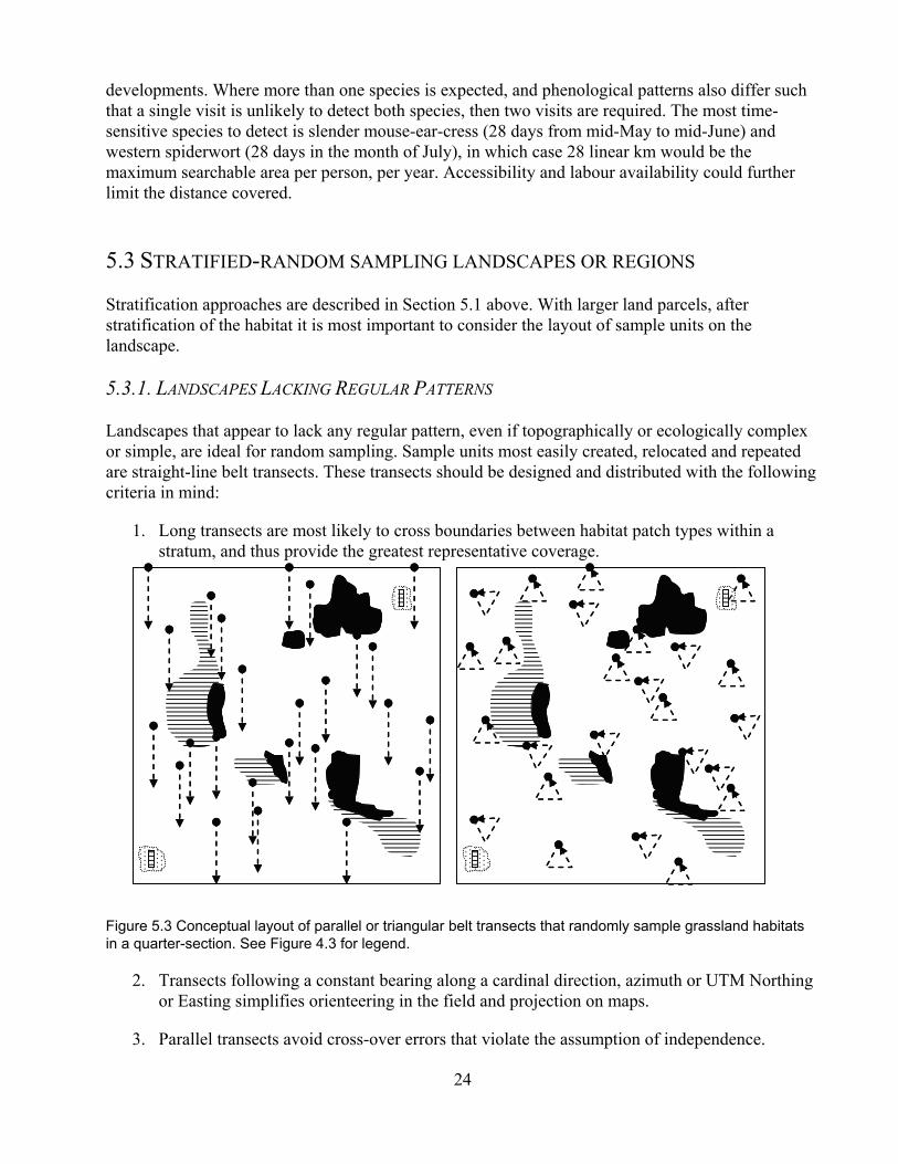
5.3 STRATIFIED-RANDOM SAMPLING LANDSCAPES OR REGIONS Stratification approaches are described in Section 5.1 above. With larger land parcels, after stratification of the habitat it is most important to consider the layout of sample units on the landscape. 5.3.1. LANDSCAPES LACKING REGULAR PATTERNS Landscapes that appear to lack any regular pattern, even if topographically or ecologically complex or simple, are ideal for random sampling. Sample units most easily created, relocated and repeated are straight-line belt transects. These transects should be designed and distributed with the following criteria in mind:
1. Long transects are most likely to cross boundaries between habitat patch types within a stratum, and thus provide the greatest representative coverage.
Figure 5.3 Conceptual layout of parallel or triangular belt transects that randomly sample grassland habitats in a quarter-section. See Figure 4.3 for legend.
2. Transects following a constant bearing along a cardinal direction, azimuth or UTM Northing or Easting simplifies orienteering in the field and projection on maps.
3. Parallel transects avoid cross-over errors that violate the assumption of independence.

25
An alternative approach to straight-line transects is a triangular configuration of belt transects, which are most efficient because a surveyor begins and ends a search at the same point (Figure 5.3). Where a surveyor is using a vehicle or ATV to travel between sample units on a large landscape, triangular belt transects may be preferred. Orienteering will be more difficult, and random start points that result in cross-over errors with nearby sample units will need to be eliminated or the randomization procedure constrained to otherwise avoid overlap. 5.3.2 REGULARLY PATTERNED LANDSCAPES Landscapes with repeated topographic or ecological pattern present special cases for sampling that require special techniques. Examples of these patterned landscapes include ridged end-moraines, sand dune complexes, glacial lake beach ridges and patterned fens. Autocorrelation of a sample unit arrangement with the underlying landscape pattern can unintentionally under-sample or over-sample a habitat type and violate the assumptions of randomization. To avoid this problem on patterned landscapes, the following approaches are recommended:
1. Where habitat requirements are poorly understood, parallel belt transects should be purposefully oriented perpendicular to the landscape pattern to bisect all possible habitats in proportion to their occurrence (Figure 5.4).
Figure 5.4 Conceptual layout of sample units oriented perpendicular to the underlying landscape pattern of sand dunes (samples grasslands and dunes) in a quarter-section.
2. Where habitat requirements are very well known, sampling can be restricted to only the preferred habitats, and either belt transects are oriented parallel to the pattern, or census-surveys are conducted in a random sample of habitat polygons.
500 m500 m
Tree & Shrub Cover
Grassland
Grassland (sand)
Wetland
Tree & Shrub Cover
Grassland
Grassland (sand)
Wetland

26
There is a natural temptation to search the more obvious and easily identified patterns in the landscape, but this assumes the surveyor has perfect knowledge of habitat preference for the targeted species. A sand dune specialist can occur on bare soil created by animal mounds or interspersed with other vegetation in interdunal swales, but no one will know if that habitat remains unsampled. 5.3.3 VALLEY OR WETLAND COMPLEXES Valley complexes provide many habitats varying in slope aspect, slope gradient, elevation and geological soil parent material. Wetlands are additionally affected by hydrologic regime, salinity and permanence of the water. Sampling for a rare species must take into account the degree of uncertainty of habitat preference information and the natural tendencies of surveyors that are not provided detailed direction.
1. Where habitat preference is poorly understood an ideal approach is to establish sample plots that include all or stratified among all slope positions or wetland zones (Figure 5.5). The search pattern within the plot should follow a parallel and adjacent transect pattern oriented perpendicular to the slope or wetland gradient, and surveyors then switch-back from the top to the bottom of the slope for ease of travel and least erosional impact (relative to uphill and downhill directions).
Figure 5.5 Conceptual layout of sample units within a valley complex that occupies a quarter-section. Numbers indicate the strategies outlined in Section 5.3.3.
2. If a species consistently occupies one particular exposed geological strata or wetland zone, it makes sense to search transects within those strata and perpendicular to the slope or wetland gradient. The search pattern is easy to travel and has minimal erosion impact (relative to uphill and downhill directions).
500 m
3
1
2
1
2
500 m
3
1
2
1
2
3
1
2
1
2

27
3. If a species consistently occupies colluvial or alluvial deposits in a valley complex (i.e., Buffalograss) or alkaline flats with indicator halophytes (i.e., alkaline wing-nerved moss) it makes sense to search transects within those strata only.
Figure 5.6 Cluster sampling of quarter-sections that were census-searched for presence or absence on available native grassland habitat in a 100 km2 study area. Cluster sampling is incomplete and will continue over a period of years until the extent of occurrence is known.
10 km
x
Native grassland
Sampled – present
Sampled – absent
x
xx
x
x
xx
x
x
xx
Urban
Lands
10 km10 km
x
Native grassland
Sampled – present
Sampled – absentx
Native grassland
Sampled – present
Sampled – absent
x
xx
x
x
xx
x
x
xx
Urban
Lands
x
xx
x
x
xx
x
x
xx
Urban
Lands

28
5.4 PHASED OR ADAPTIVE CLUSTER-SAMPLING LANDSCAPES Very large study areas present a number of logistical challenges that require special consideration to ensure project objectives are realistic and survey effort is adequate. Some simple solutions to this problem are to reduce the extent of the study area, or subdivide the study area or collection of sample units and complete the project in phases over multiple years. Dispersal-limitations of rare plant species often lead to a clustered regional distribution, and sampling methods have been developed to accommodate this reality. Adaptive cluster sampling involves a random sampling phase followed by a cluster sampling phase (Thompson 1991; Acharya et al. 2000), which more rapidly reveals the EOO and AOO of a rare plant species (Smith et al. 2004).
1. In the first phase, random sampling of the study area proceeds. If no occurrences are found, the intensity of the random sampling can be increased by addition of more randomly located sample units. If an occurrence is found, random sampling ceases and a second phase of cluster sampling begins.
2. In the second phase, additional sample units are purposely placed adjacent to and
surrounding the sample units containing occurrences. If more occurrences are found in those adjacent sample units, this adaptive process will continue until a peripheral ring of absent sample units is created.
If a very small proportion of the landscape or region was sampled, the process can continue with random sampling until another occurrence is encountered, followed by implementation of additional cluster sampling. Where it is more important to find all the occurrences to protect them from an immediate threat, adaptive cluster sampling may be the most efficient tool. For further efficiency, once an occurrence is discovered inside a sample unit the remainder of that unit does not need to be sampled. Instead, it is more efficient to move on to an adjacent sample unit to increase knowledge of EOO and AOO (Smith et al. 2004). This approach has been implemented at the scale of a 100 km2 municipality in southeastern Saskatchewan to find buffalograss (Buchloe dactyloides) at the scale of quarter-section sample units (Figure 5.6). Additional survey work occurs each year to build on previous surveys and as a result has expanded the known EOO and AOO each year.
29
6.0 DOCUMENTING SEARCH-EFFORT AND ABSENCE DATA
6.1 SIMPLE DOCUMENTATION Search-effort calculations can be partially completed in advance of a survey by first documenting the size and area of survey units. The second step is simply to record the start and end times for surveying each unit. Finally, enough information will be collected to calculate an area searched by unit time (i.e., m2/minute, or hectares/hour), or time required to search a unit of area (i.e., seconds/m2, or hours/hectare). Where many survey units exist, it is also possible to calculate measures of central tendency, range and variation. Absence information is most easily calculated as the area of all sample units minus the area occupied by plant occurrences. Where a survey resulted in no new rare plant records, the entire study design can serve as an absence data set with coordinates for transects or plot boundaries. Future surveys may choose to resample the same transects to estimate detectability or changes in distribution over time, so careful description and documentation of all survey units is absolutely important regardless of whether a plant was found the first time around.
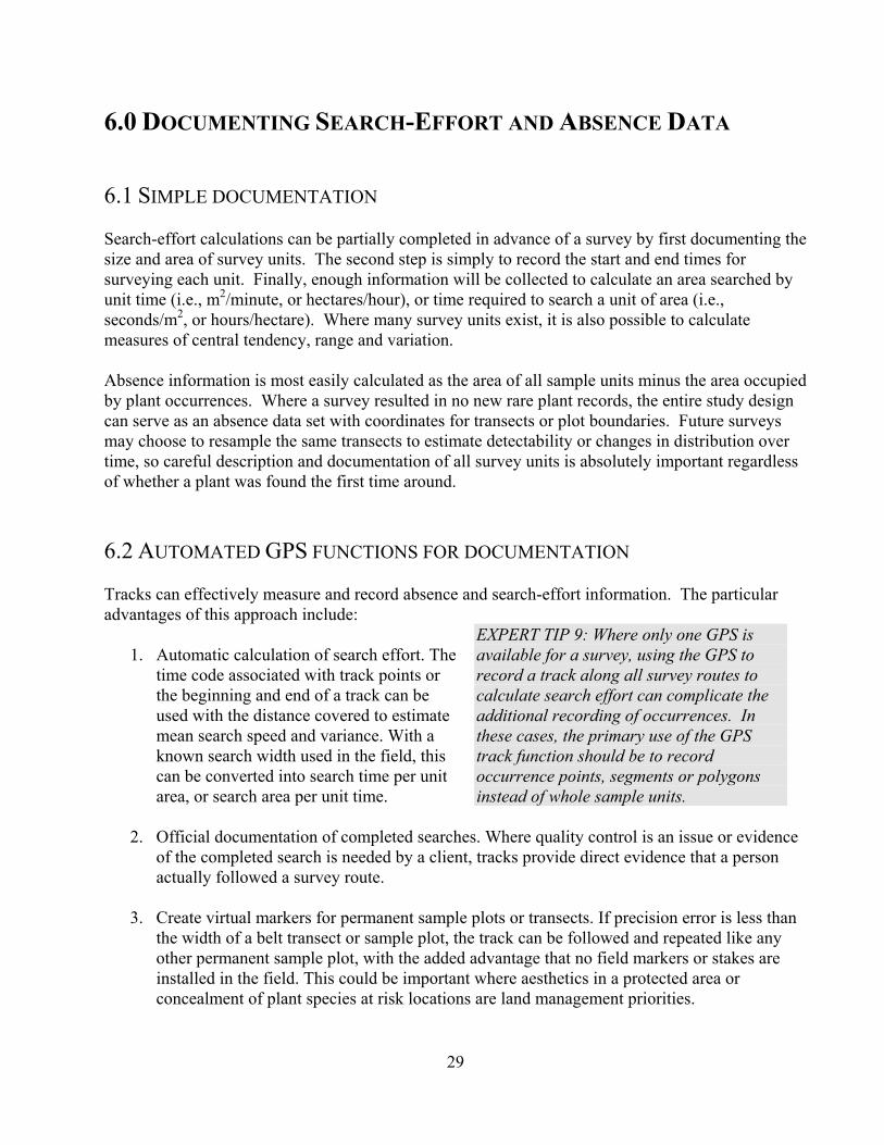
6.2 AUTOMATED GPS FUNCTIONS FOR DOCUMENTATION Tracks can effectively measure and record absence and search-effort information. The particular advantages of this approach include:
1. Automatic calculation of search effort. The
time code associated with track points or the beginning and end of a track can be used with the distance covered to estimate mean search speed and variance. With a known search width used in the field, this can be converted into search time per unit area, or search area per unit time.
EXPERT TIP 9: Where only one GPS is available for a survey, using the GPS to record a track along all survey routes to calculate search effort can complicate the additional recording of occurrences. In these cases, the primary use of the GPS track function should be to record occurrence points, segments or polygons instead of whole sample units.
2. Official documentation of completed searches. Where quality control is an issue or evidence of the completed search is needed by a client, tracks provide direct evidence that a person actually followed a survey route.
3. Create virtual markers for permanent sample plots or transects. If precision error is less than
the width of a belt transect or sample plot, the track can be followed and repeated like any other permanent sample plot, with the added advantage that no field markers or stakes are installed in the field. This could be important where aesthetics in a protected area or concealment of plant species at risk locations are land management priorities.

30
4. Identifies logistical problems with pre-planned straight-line transects. There will always be cases where a pre-planned linear transect cannot be followed, because hazards or barriers prevent surveyors from following the route. Those problems can be identified to adjust future plans to resample the area, or to specifically exclude areas from analytical extrapolation that will never be surveyed for confirmation.
0 50 10025 m
Figure 6.1 Survey track surrounding a constructed wetland (dugout impoundment on a coulee) in southeastern Saskatchewan. The objective was to complete a census-survey for buffalograss on accessible terrain within 75 m of the centre point of each dugout or similar wetland. The pattern follows a switch-back down steep coulee slopes toward the wetland edge, and across the coulee bottom downstream of the impoundment. Cross-over errors result from changing satellite reception as the surveyor on the ground used pin-flags to definitively avoid these errors and walk straight lines (data source: Environment Canada).
Survey area
(75 m radius)
Streamflow
direction
DUGOUT

31
7.0 MANAGING AND REPORTING PROJECT DATA
7.1 DATA STRUCTURE AND RELATIONAL TABLES Every rare plant survey will generate several kinds of data that can be kept in separate data files or tables. By keeping these data files separate but relational, projects can be more easily repeated for verification or monitoring, or expanded to more species or larger areas at some future point. No software recommendations are suggested, but database files create more secure records that are difficult to accidentally sort or otherwise edit in a way that renders them useless. The following data file contents are suggested for projects:
1. Observer Information: Each person conducting surveys should be identified by a unique observer code for the census or sample locations he or she visit (see below). This code can be related to this observer information table, where contact information and qualifications for that observer can be included for later reference.
2. Study Area Boundaries: This can be a spatial layer (i.e., GIS shapefile) or a tabular list of
coordinates that outline a polygon for the study area (i.e., spreadsheet). This can form the base map or mask for any GIS project associated with the survey.
3. Census or Sampling Station Locations: These can also be spatial or tabular data (points,
lines, polygons), and represent the smallest units to be surveyed for a given species, nested within the study area boundaries. In the case of census-surveys, these may be cells in a grid or adjacent rectangular polygons, while sampling-surveys may have discrete sampling plots, belt or line transects that do not share boundaries. Each station can be visited several times by different observers, and within each station the rare plant occurrences may appear, disappear, expand or contract over time.
4. Visits: Only where a project involves repeated sampling of the same units would this
information be recorded. This could be as simple as a yes/no answer for a given year, or as detailed as a GPS track file documenting the actual searched route inside each unit at each interval.
5. Occurrences: Many options are available to record occurrence information.
a) Where census or sample station locations are small enough, it may be sufficient to indicate presence or absence for each visit of a unit as a single digit (0 or 1). This works best where sample units are smaller than the typical patch size.
b) Where one or more segments of a single belt transect contains or intersects one or more occurrences, it may be sufficient to indicate the starting and ending coordinates of each segment within each transect for each visit. With parallel and adjacent transects in a census-survey, the coordinates will automatically outline the polygon boundaries of each occurrence.

32
c) When sampling, the occurrence may overlap into unsurveyed territory on either side of a belt transect or sample plot. Depending upon the objectives of the project there are two options:
1. To extrapolate the occurrence using presence and absence data within sample units, it is only important to record the occupied segment following the method in 5.b) above.
2. Sometimes the sampling regime is really a means to locate occurrences, with the real objective to map the boundary of occurrences inside and outside of the original sample unit. This data may require many rows for coordinates in a vector polygon or cells in a raster polygon, or could be identified by a unique shapefile name that is located elsewhere. An overlay of this data will also satisfy the objective in 5.c)1. above.
Relates to separate table Relates to separate table Starting and ending Eastings describing the Study Area describing the Observer describing segments of a belt transect that is occupied
STUDY STATION OBSERVER VISIT SPECIES START E END E SUFFIELD NWA004 DCH 12/06/08 CRYMIN 560870 560890 SUFFIELD NWA004 DCH 06/06/09 CRYMIN 560875 560885 SHILO E1006 CLN 16/08/06 DALVIL 456090 456095
Relates to separate table Entry unto itself or Code for the target describing the sampling related to a separate rare plant species Station position table of the track Figure 7.1 Example layout of an occurrence data table with fields identifying study area, station, observer and visit information contained in separate but related data tables.
7.2 MINIMUM DATA SET TO REPORT In order to demonstrate a survey project was designed as objectively as possible, is described sufficiently to repeat the work, and data summaries provide meaningful information for status assessment updates and future monitoring efforts, there is a minimum data set to report. A Materials and Methods section should include the following: Map of the study area, any strata and arrangement of survey routes within the study area.
Tables with coordinates outlining study area, strata and survey boundaries (see Section 7.1).
Equations or references thereto for all calculations undertaken.
Units for all numerical values reported, including significant digits if necessary.

33
Calendar dates of all surveys undertaken in the field.
Definition of an occurrence in light of the study design.
A Results section should include all or some of the following, where appropriate: Search effort in time per unit area, or area per unit time. Include an appropriate statistical estimate
for central tendency, range and variance in the search effort data.
Number of occurrences. Include an estimate for central tendency, range and variance.
Element occurrence record numbers from previous surveys that are associated with the
occurrences found and described in this survey.
Area of occupancy. Include an estimate for central tendency, range and variance.
Detection probability in units of percent or decimal proportion. Include an estimate for central
tendency, range and variance.

34
8.0 ACKNOWLEDGEMENTS The Recovery Team for Plant Species at Risk in the Prairie Provinces identified the need for standardized inventory and monitoring protocols at several meetings between 2004 and 2006. That team included Dean Nernberg and Candace Neufeld (Environment Canada), Jason Greenall (Manitoba Conservation), Robin Gutsell and Joel Nicholson (Alberta Sustainable Resource Development), Sue McAdam (Saskatchewan Environment), Chris Nykoluk (Agriculture and Agri-food Canada’s Agri-Environmental Services Branch, formerly Prairie Farm Rehabilitation Administration), Peggy Strankman (Canadian Cattlemen’s Association), and Cheryl-Ann Beckles, Delaney Boyd, and Sherry-Lynn Punak-Murphy (Department of National Defence). Jennifer Neudorf undertook efforts to make species-specific detectability guidelines in 2005, which then evolved into a joint effort to create inventory and monitoring guidelines with Darcy Henderson in 2006. That first draft was reviewed in 2007 by Bob Godwin (Saskatchewan Research Council), Jennifer Rowland (Department of National Defence), Jennifer Doubt (Canadian Museum of Nature), Joyce Gould (Alberta Sustainable Resource Development), Bret Ward (Agriculture and Agri-food Canada’s Agri-Environmental Services Branch, formerly Prairie Farm Rehabilitation Administration), Wade Sumner (MDH Solutions Inc.), Diana Bizecki-Robson (Manitoba Museum of Man and Nature), Renny Grilz and Cary Hamel (Nature Conservancy of Canada), Catherine Foster (Manitoba Conservation), Richard St. Pierre (Plant Gene Resources Canada), and Lisa Matthias (Alberta Sustainable Resource Development). The results of these reviews, and the field testing of methods with contractors and summer students in 2007 and 2008 helped change and improve a second and third draft in innumerable ways. Special thanks are owed to Candace Neufeld, Monika Tan, Robin Bloom, Rachel Banting, Bob Godwin, Anna Leighton and Beryl Waite for useful insights.

35
9.0 REFERENCES
Acharya, B., Bhattarai, B., de Gier, A. and Stein, A. 2000. Systematic adaptive cluster sampling for the assessment of rare tree species in Nepal. Forest Ecology and Management 137: 65-73.
Alberta Native Plant Council. 2006. Plant collection guidelines for researchers, students and consultants, Version 2. Alberta Native Plant Council. Edmonton AB.
Archaux, F., Gosselin, F., Berges, L., Chevalier, R. 2006. Effects of sampling time, species richness and observer on the exhaustiveness of plant censuses. Journal of Vegetation Science. 17: 299-306.
Archaux, F., Camaret, S., Dupouey, J-L., Ulrich, E., Corcket, E., Bourjot, L. Brethes, A., Chevalier, R., Dobremez, J-F., Dumas, Y, Dume, G., Foret, M., Forgeard, F., Lebret-Gallet, M., Picard, J-F., Richard, F., Savoie, J-M., Seytre, L. Timbal, J., Touffet, J. 2009. Can we reliably estimate species richness with large plots? An assessment through calibration training. Plant Ecology. 203: 303-315.
Argus, G.W. and White, D.J. 1978. The rare vascular plants of Alberta. Syllogeus No. 17. National Museum of Natural Sciences. Ottawa ON.
BC Ministry of Environment, Lands and Parks. 1998. Species inventory fundamentals: standards for components of British Columbia’s biodiversity No. 1. Terrestrial Ecosystems Task Force, Resources Inventory Committee, BC Ministry of Environment, Lands and Parks. Victoria BC.
Bizecki-Robson, D. 2000. Guidelines for rare plant surveys. Native Plant Society of Saskatchewan. Saskatoon SK.
California Native Plant Society. 2001. CNPS botanical survey guidelines. Pp. 38-40 In: Tibor, D.P. (ed). California Native Plant Society’s inventory of rare and endangered vascular plants of California, sixth edition. Special Publication No. 1. California Native Plant Society. Sacramento CA.
COSEWIC 2006. COSEWIC’s assessment process and criteria. Committee on the Status of Endangered Wildlife in Canada. Canadian Wildlife Service, Environment Canada. Ottawa ON.
Edwards, T.C. Jr., Cutler, D.R., Zimmermann, N.E., Geiser, L. and Moisen, G.G. 2006. Effects of sample survey design on the accuracy of classification tree models in species distribution models. Ecological Modeling. 199: 132-141.
Elzinga, C.L., Salzer, D.W., Willoughby, J.W. 2001. Measuring and monitoring plant populations. U.S. Bureau of Land Management Technical Reference 1730-1. Denver CO.
Fancy, S.G. 2000. Guidance for the design of sampling schemes for inventory and monitoring of biological resources in National Parks. National Park Service Inventory and Monitoring Program.
Godwin, B., Thorpe, J. 2007. Targeted surveys for plant species at risk in Elbow, Dundurn, and Rudy-Rosedale AAFC-PFRA Pastures, 2006. Saskatchewan Research Council Publication No. 11997-1E07. Saskatoon SK.
Government of Canada. 2002. Species at Risk Act. Statutes of Canada 2002, Chapter 29, An Act respecting the protection of wildlife species at risk in Canada. Bill C-5. Assented to 12th December, 2002. Ottawa ON.
Government of Saskatchewan. 2007. The Great Sand Hills Regional Environmental Study: Final Report. Government of Saskatchewan report 2007-104. Regina SK.
Johnson, S.E., Mudrak, E.L., Beever, E.A., Sanders, S. and Waller, D.M. 2008. Comparing power among three sampling methods for monitoring forest vegetation. Canadian Journal of Forest Research. 38: 143-156.
Joseph, L.N., Field, S.A., Wilcox, C. and Possingham, H.P. 2006. Presence-absence versus abundance data for monitoring threatened species. Conservation Biology 20: 1679-1687.
Kercher, S.M., Frieswyk, C.B., Zedler, J.B. 2003. Effects of sampling teams and estimate methods on the assessment of plant cover. Journal of Vegetation Science. 14: 899-906.
Kershaw, L., Gould, J., Johnson, D. and Lancaster, J. 2001. Rare vascular plants of Alberta. University of Alberta Press. Edmonton AB.

36
Kery, M. 2004. Extinction rate estimates for plant populations in revisitation studies: importance of detectability. Conservation Biology. 18: 570-574.
Kirk, D. 2004. Guidance for inventory and monitoring of species at risk on Environment Canada federal lands. Canadian Wildlife Service.
Klimes, L. 2003. Scale-dependent variation in visual estimates of grassland plant cover. Journal of Vegetation Science. 14: 815-821.
Lancaster, J. 2000. Guidelines for rare plant surveys. Alberta Native Plant Council. Edmonton AB.
MacKenzie, D.I. and Royle, J.A. 2005. Designing occupancy studies: general advice and allocating survey effort. Journal of Applied Ecology. 42: 1105-1114.
MacKenzie, D.I., Nichols, J.D., Lachman, G.B., Droege, S., Royle, J.A. and Langtimm, C.A. 2002. Estimating site occupancy rates when detection probabilities are less than one. Ecology 83: 2248-2255.
Maher, R.V., Argus, G.W., Harms, V.L. and Hudson, J.H. 1979. The rare vascular plants of Saskatchewan. Syllogeus No. 20. National Museum of Natural Sciences. Ottawa ON.
McDonald, L.L. 2004. Sampling rare populations. Pp. 11-42 in Thompson, W.L. (ed.) Sampling rare or elusive species: Concepts, designs, and techniques for estimating population parameters. Island Press. Covelo CA.
Menges, E.S., Guerrant, E.O. Jr., and Hamze, S. 2004. Effects of seed collection on the extinction risk of perennial plants. Pp. 305-324 in Guerrant, E.O. Jr., Havens, K. and Maunder, M. (eds). Ex situ plant conservation: Supporting species survival in the wild. Society for Ecological Restoration International and Center for Plant Conservation. Island Press. Covelo CA.
Milberg, P., Bergstedt, J., Fridman, J., Odell, G., Westerberg, L. 2008. Observer bias and random variation in vegetation monitoring data. Journal of Vegetation Science 19: 633-644.
Moerman, D.E. and Estabrook, G.F. 2006. The botanist effect: Counties with maximal species richness tend to be home to universities and botanists. Journal of Biogeography. 33: 1969-1974.
NatureServe. 2004. NatureServe benchmark data content standards. NatureServe. Arlington VA.
Pollock, K.H., Marsh, H., Bailey, L.L., Farnsworth, G.L., Simons, T.R. and Alldredge, M.W. 2004. Separating components of detection probability in abundance estimation: An overview with diverse examples. Pp. 43-58 in Thompson, W.L. (ed.) Sampling rare or elusive species: Concepts, designs, and techniques for estimating population parameters. Island Press. Covelo CA.
Rondinini, C., Wilson, K.A., Boitani, L., Grantham, H. and Possingham, H.P. 2006. Tradeoffs of different types of species occurrence data for use in systematic conservation planning. Ecology Letters. 9: 1136-1145.
Smith, D.R., Brown, J.A. and Lo, N.C.H. 2004. Application of adaptive sampling to biological populations. Pp. 77-122 in Thompson, W.L. (ed.) Sampling rare or elusive species: Concepts, designs, and techniques for estimating population parameters. Island Press. Covelo CA.
Stohlgren, T. J. 2006. Measuring plant diversity; lessons from the field. Oxford University Press. New York.
Thompson, S.K. 1991. Adaptive cluster sampling: Designs with primary and secondary units. Biometrics. 47: 1103.
Thompson, W.L. (ed.) 2004. Sampling rare or elusive species: Concepts, designs, and techniques for estimating population parameters. Island Press. Covelo CA.
Vesely, D. McComb, B.C., Vojta, C.D., Suring, L.H., Halaj, J., Holthausen, R.S., Zuckerberg, B., Manley, P.M. 2006. Development of Protocols To Inventory or Monitor Wildlife, Fish, or Rare Plants. Gen. Tech. Rep. WO-72. U.S. Department of Agriculture – Forest Service. Washington DC.
Vittoz, P. Guisan, A. 2007. How reliable is the monitoring of permanent vegetation plots? A test with multiple observers. Journal of Vegetation Science. 18: 413-422.
Wallis, C. 2001. Proposed protocols for inventories of rare plants of the Grassland Natural Region. Alberta Species at Risk Report No. 21. Alberta Sustainable Resource Development, Fish and Wildlife Service. Edmonton AB.
White, D.J. and Johnson, K.L. 1980. The rare vascular plants of Manitoba. Syllogeus No. 27. National Museum of Natural Sciences. Ottawa ON.

37
10.0 APPENDIX A: PLANT SPECIES AT RISK RESOURCES Plant species at risk in the Prairie Ecozone afforded protection under the Species at Risk Act.
Common Name Scientific Name Status 2007 Life History and Form Rough agalinis Agalinis aspera Endangered Annual Gattinger’s agalinis Agalinis gattingerii Endangered Annual Small-flowered sand-verbena Tripterocalyx micranthus Endangered Annual Small white lady’s slipper Cypripedium candidum Endangered Perennial, herbaceous Tiny cryptanthe Cryptantha minima Endangered Annual Western prairie fringed orchid Platanthera praeclara Endangered Perennial, herbaceous Buffalograss Buchloë dactyloides Threatened Perennial, herbaceous Hairy prairie-clover Dalea villosa var. villosa Threatened Perennial, herbaceous Slender mouse-ear-cress Halimolobos virgata Threatened Biennial Smooth goosefoot Chenopodium subglabrum Threatened Annual Soapweed (Yucca) Yucca glauca Threatened Perennial, evergreen Western blue flag Iris missouriensis Threatened Perennial, herbaceous Western silvery aster Symphyotrichum sericeum Threatened Perennial, herbaceous Western spiderwort Tradescantia occidentalis Threatened Perennial, herbaceous COSEWIC (learn about the Canadian species at risk assessment process) www.cosewic.gc.ca SARA Public Registry (find all status reports, recovery strategies, permits and policies) www.sararegistry.gc.ca NatureServe Canada (learn about their conservation ranking process and resources) www.natureserve-canada.ca Manitoba Conservation Data Centre (element occurrence records for Manitoba) http://web2.gov.mb.ca/conservation/cdc Saskatchewan Conservation Data Centre (element occurrence records for Saskatchewan) www.biodiversity.sk.ca Alberta Natural Heritage Information Centre (element occurrence records for Alberta) http://tpr.alberta.ca/parks/heritageinfocentre/default.aspx