Occupant Behaviour Prediction in Ambient … M. J. Akhlaghinia1 et al.：Occupant Behaviour Prediction in Ambient Intelligence Computing Environment the main focus of this article,

858585858516

Journal of Uncertain SystemsVol.2, No.2, pp.85-100, 2008

Online at: www.jus.org.uk

Occupant Behaviour Prediction in Ambient Intelligence

Computing Environment

M. Javad Akhlaghinia*, Ahmad Lotfi, Caroline Langensiepen, Nasser Sherkat School of Computing and Informatics

Nottingham Trent University, Clifton Campus, Nottingham, NG118NS, United Kingdom

Received 20 July 2007; Accepted 25 December 2007

Abstract

In this paper, the application of ambient intelligence computing techniques in the prediction of occupant behaviours is addressed. It is aimed to deliver a wellbeing monitoring and assistive environment to support elderly lives independently, in control of their day to day activities. A wireless sensor network is constructed to collect the required occupancy data. Individual sensory data are combined to form an occupancy time series. In this paper different techniques in time series prediction are investigated. The prediction techniques include an Evolving Fuzzy Predictor (EFP) model along with Auto Regressive Moving Average (ARMA) model, Adaptive-Network-based Fuzzy Inference System (ANFIS), as well as Transductive Neuro-Fuzzy Inference model with Weighted data normalization (TWNFI). These prediction techniques are used to predict the occupancy time series representing anticipated occupancy of different areas of the environment, and the results are compared. Experimental results are presented based on a home environment with four separate areas and each area is equipped with a wireless passive infrared motion detector linked to a central processing unit. For wireless communication of the sensor network, ZigBee wireless modules are employed in the prototype ambient intelligence environment.

© 2008 World Academic Press, UK. All rights reserved. Keywords: ambient intelligence, computational intelligence, Wireless Sensor Network (WSN), time series, prediction, evolving, fuzzy, neuro-fuzzy, Auto Regressive Moving Average (ARMA)

1 Introduction It is always useful to be able to predict a particular event in the future in more certain terms rather than a forecast. Prediction techniques have been applied in different areas of science and technology. In financial systems, for example, stock market prediction has attracted a great deal of attention. In mechanical and electrical systems, condition monitoring and predictive maintenance have the benefit of determining the condition of in-service equipment and providing an accurate alarm before a fault reaches critical level [1].

In this paper, it is intended to investigate prediction techniques in a smart home environment where the behaviours of occupants are predicted. This kind of smart environment is called a predictive ambient intelligence environment, which can be categorized as the new third generation of smart environments [2]. The new emerging third generation of smart environments also known as predictive ambient intelligence environments can learn from environmental changes as well as behavioural patterns of occupants.

Predictive ambient intelligence environments collect data acquired from a sensor network. Collected data include a variety of attributes, such as the environmental changes and occupants’ interactions with the environment. These data are used in a learning approach to make a predictive ambient intelligence environment that can predict the occupancy of different areas, as well as requirements and interests of occupants at different times. This predictive feature, for example, can improve the performance of energy saving approaches in a smart environment; in addition, it enhances the convenience of occupants as well as security and safety.

Data collection and prediction are two key challenges of predictive ambient intelligence environments. The first challenge is due to the energy and bandwidth constraints in sensor networks [3, 4], but the second challenge, which is

* Corresponding author. Email: [email protected]. (M. J. Akhlaghinia)

M. J. Akhlaghinia1 et al.：Occupant Behaviour Prediction in Ambient Intelligence Computing Environment 86

the main focus of this article, is a learning problem in distributed sensor networks. A predictive ambient intelligence environment can predict the next state of consecutive interactions with the use of the knowledge it has learnt from previously observed interactions. For instance, it can predict the favourite light intensity of different occupants in a specific area of the environment at a specific time of a day. Prediction consists of pattern extraction to identify sequences of actions, and then sequence matching to predict the next action in one of these sequences [5].

The prime application of the research reported here is to deliver a wellbeing monitoring and assistive environment to support elderly people to live independently, in control and able to care for themselves within the limits of their abilities. To take into account the chaotic behaviour of the occupant, the uncertainty and anomalies of the occupant behaviour will be modelled. To achieve this goal, historical data are used as the basis for estimating occupant behaviour in future.

In this paper, as part of our ongoing research, a comprehensive comparative study is conducted to investigate different approaches available in predictive techniques in prediction of occupant behaviour. A summary of available prediction techniques focusing mainly in three areas of data mining, soft computing techniques and statistical modelling prediction techniques is reported in section 2. Section 3 covers the data acquisition technologies and the proposed data acquisition system for this research. Our proposed environment and data representation for our prediction strategy is considered in section 4. Prediction techniques are explained in Section 5 followed by experimental results in Section 6. Relevant concluding remarks and further works are discussed in the final section. 2 Prediction Techniques in Ambient Intelligence Environment Prediction in ambient environments is a learning challenge in distributed sensor networks. There are a variety of techniques for this learning challenge including data mining techniques, soft computing techniques and statistical modelling techniques. A review of these techniques is presented in this section. 2.1 Data Mining Prediction Techniques Two prediction techniques coming from the area of data mining are discussed in this section including Case-Based Reasoning and Distributed Voting Approach. Case-Based Reasoning

Case-Based Reasoning (CBR) is a classification method that uses previous experiences to find a solution for current problem. It has two basic operations including case-generation and case-selection [6]. As a method of prediction, context-aware based case-based reasoning proposed in [7] is used as a method of pattern extraction of occupants’ behaviour in a predictive ambient intelligence environment. In this method, the context in a smart home is classified into three dimensions, namely time, environment and person [8]. In this method each case is represented as follows:

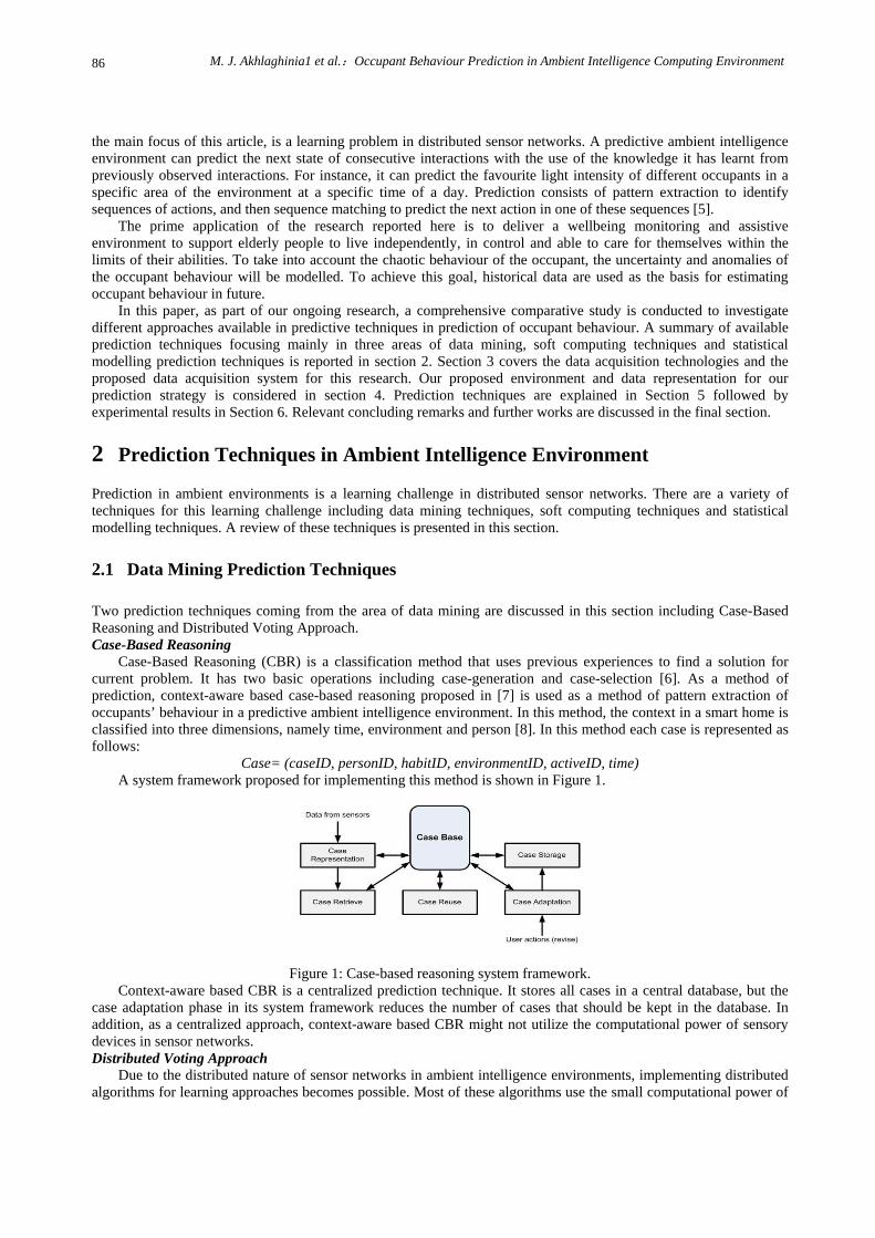
Case= (caseID, personID, habitID, environmentID, activeID, time) A system framework proposed for implementing this method is shown in Figure 1.

Figure 1: Case-based reasoning system framework. Context-aware based CBR is a centralized prediction technique. It stores all cases in a central database, but the

case adaptation phase in its system framework reduces the number of cases that should be kept in the database. In addition, as a centralized approach, context-aware based CBR might not utilize the computational power of sensory devices in sensor networks. Distributed Voting Approach

Due to the distributed nature of sensor networks in ambient intelligence environments, implementing distributed algorithms for learning approaches becomes possible. Most of these algorithms use the small computational power of

Journal of Uncertain Systems, Vol.2, No.2, pp.85-100, 2008 87

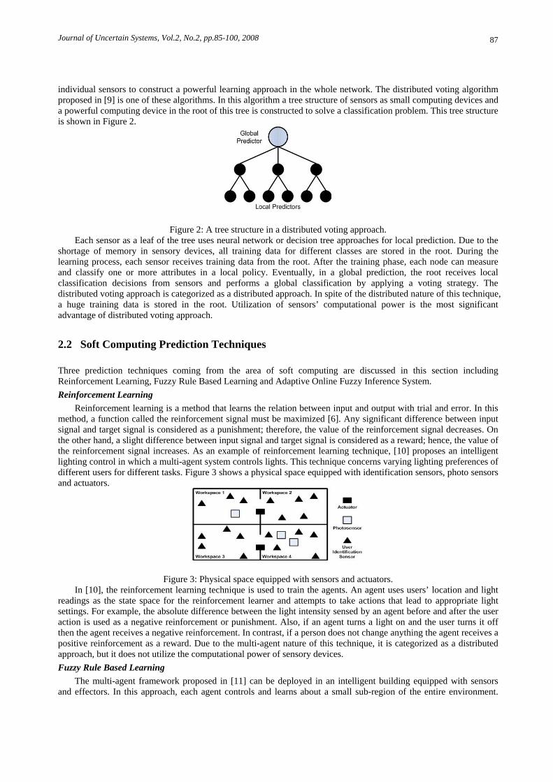
individual sensors to construct a powerful learning approach in the whole network. The distributed voting algorithm proposed in [9] is one of these algorithms. In this algorithm a tree structure of sensors as small computing devices and a powerful computing device in the root of this tree is constructed to solve a classification problem. This tree structure is shown in Figure 2.

Figure 2: A tree structure in a distributed voting approach. Each sensor as a leaf of the tree uses neural network or decision tree approaches for local prediction. Due to the

shortage of memory in sensory devices, all training data for different classes are stored in the root. During the learning process, each sensor receives training data from the root. After the training phase, each node can measure and classify one or more attributes in a local policy. Eventually, in a global prediction, the root receives local classification decisions from sensors and performs a global classification by applying a voting strategy. The distributed voting approach is categorized as a distributed approach. In spite of the distributed nature of this technique, a huge training data is stored in the root. Utilization of sensors’ computational power is the most significant advantage of distributed voting approach.

2.2 Soft Computing Prediction Techniques Three prediction techniques coming from the area of soft computing are discussed in this section including Reinforcement Learning, Fuzzy Rule Based Learning and Adaptive Online Fuzzy Inference System. Reinforcement Learning

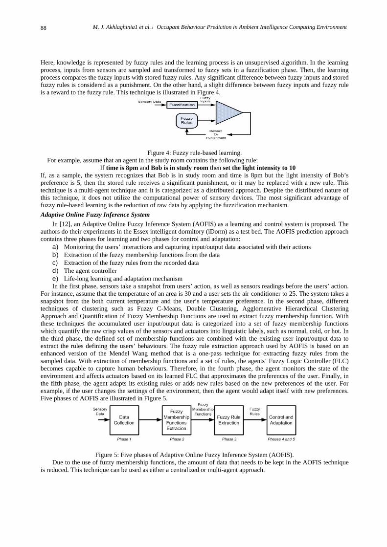
Reinforcement learning is a method that learns the relation between input and output with trial and error. In this method, a function called the reinforcement signal must be maximized [6]. Any significant difference between input signal and target signal is considered as a punishment; therefore, the value of the reinforcement signal decreases. On the other hand, a slight difference between input signal and target signal is considered as a reward; hence, the value of the reinforcement signal increases. As an example of reinforcement learning technique, [10] proposes an intelligent lighting control in which a multi-agent system controls lights. This technique concerns varying lighting preferences of different users for different tasks. Figure 3 shows a physical space equipped with identification sensors, photo sensors and actuators.

Figure 3: Physical space equipped with sensors and actuators. In [10], the reinforcement learning technique is used to train the agents. An agent uses users’ location and light

readings as the state space for the reinforcement learner and attempts to take actions that lead to appropriate light settings. For example, the absolute difference between the light intensity sensed by an agent before and after the user action is used as a negative reinforcement or punishment. Also, if an agent turns a light on and the user turns it off then the agent receives a negative reinforcement. In contrast, if a person does not change anything the agent receives a positive reinforcement as a reward. Due to the multi-agent nature of this technique, it is categorized as a distributed approach, but it does not utilize the computational power of sensory devices. Fuzzy Rule Based Learning

The multi-agent framework proposed in [11] can be deployed in an intelligent building equipped with sensors and effectors. In this approach, each agent controls and learns about a small sub-region of the entire environment.


Here, knowledge is represented by fuzzy rules and the learning process is an unsupervised algorithm. In the learning process, inputs from sensors are sampled and transformed to fuzzy sets in a fuzzification phase. Then, the learning process compares the fuzzy inputs with stored fuzzy rules. Any significant difference between fuzzy inputs and stored fuzzy rules is considered as a punishment. On the other hand, a slight difference between fuzzy inputs and fuzzy rule is a reward to the fuzzy rule. This technique is illustrated in Figure 4.

Figure 4: Fuzzy rule-based learning. For example, assume that an agent in the study room contains the following rule:

If time is 8pm and Bob is in study room then set the light intensity to 10 If, as a sample, the system recognizes that Bob is in study room and time is 8pm but the light intensity of Bob’s preference is 5, then the stored rule receives a significant punishment, or it may be replaced with a new rule. This technique is a multi-agent technique and it is categorized as a distributed approach. Despite the distributed nature of this technique, it does not utilize the computational power of sensory devices. The most significant advantage of fuzzy rule-based learning is the reduction of raw data by applying the fuzzification mechanism. Adaptive Online Fuzzy Inference System

In [12], an Adaptive Online Fuzzy Inference System (AOFIS) as a learning and control system is proposed. The authors do their experiments in the Essex intelligent dormitory (iDorm) as a test bed. The AOFIS prediction approach contains three phases for learning and two phases for control and adaptation:

a) Monitoring the users’ interactions and capturing input/output data associated with their actions b) Extraction of the fuzzy membership functions from the data c) Extraction of the fuzzy rules from the recorded data d) The agent controller e) Life-long learning and adaptation mechanism In the first phase, sensors take a snapshot from users’ action, as well as sensors readings before the users’ action.

For instance, assume that the temperature of an area is 30 and a user sets the air conditioner to 25. The system takes a snapshot from the both current temperature and the user’s temperature preference. In the second phase, different techniques of clustering such as Fuzzy C-Means, Double Clustering, Agglomerative Hierarchical Clustering Approach and Quantification of Fuzzy Membership Functions are used to extract fuzzy membership function. With these techniques the accumulated user input/output data is categorized into a set of fuzzy membership functions which quantify the raw crisp values of the sensors and actuators into linguistic labels, such as normal, cold, or hot. In the third phase, the defined set of membership functions are combined with the existing user input/output data to extract the rules defining the users’ behaviours. The fuzzy rule extraction approach used by AOFIS is based on an enhanced version of the Mendel Wang method that is a one-pass technique for extracting fuzzy rules from the sampled data. With extraction of membership functions and a set of rules, the agents’ Fuzzy Logic Controller (FLC) becomes capable to capture human behaviours. Therefore, in the fourth phase, the agent monitors the state of the environment and affects actuators based on its learned FLC that approximates the preferences of the user. Finally, in the fifth phase, the agent adapts its existing rules or adds new rules based on the new preferences of the user. For example, if the user changes the settings of the environment, then the agent would adapt itself with new preferences. Five phases of AOFIS are illustrated in Figure 5.

Figure 5: Five phases of Adaptive Online Fuzzy Inference System (AOFIS). Due to the use of fuzzy membership functions, the amount of data that needs to be kept in the AOFIS technique

is reduced. This technique can be used as either a centralized or multi-agent approach.


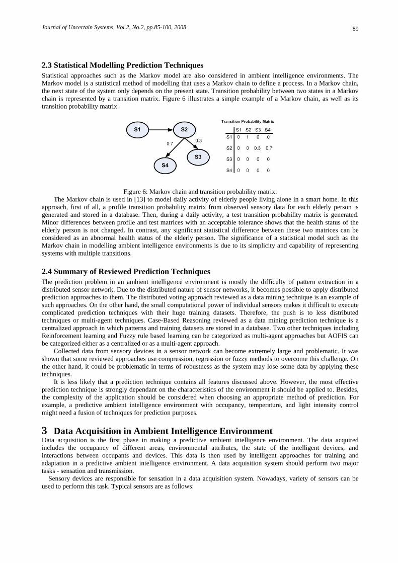
2.3 Statistical Modelling Prediction Techniques Statistical approaches such as the Markov model are also considered in ambient intelligence environments. The Markov model is a statistical method of modelling that uses a Markov chain to define a process. In a Markov chain, the next state of the system only depends on the present state. Transition probability between two states in a Markov chain is represented by a transition matrix. Figure 6 illustrates a simple example of a Markov chain, as well as its transition probability matrix.

Figure 6: Markov chain and transition probability matrix. The Markov chain is used in [13] to model daily activity of elderly people living alone in a smart home. In this

approach, first of all, a profile transition probability matrix from observed sensory data for each elderly person is generated and stored in a database. Then, during a daily activity, a test transition probability matrix is generated. Minor differences between profile and test matrices with an acceptable tolerance shows that the health status of the elderly person is not changed. In contrast, any significant statistical difference between these two matrices can be considered as an abnormal health status of the elderly person. The significance of a statistical model such as the Markov chain in modelling ambient intelligence environments is due to its simplicity and capability of representing systems with multiple transitions.

2.4 Summary of Reviewed Prediction Techniques The prediction problem in an ambient intelligence environment is mostly the difficulty of pattern extraction in a distributed sensor network. Due to the distributed nature of sensor networks, it becomes possible to apply distributed prediction approaches to them. The distributed voting approach reviewed as a data mining technique is an example of such approaches. On the other hand, the small computational power of individual sensors makes it difficult to execute complicated prediction techniques with their huge training datasets. Therefore, the push is to less distributed techniques or multi-agent techniques. Case-Based Reasoning reviewed as a data mining prediction technique is a centralized approach in which patterns and training datasets are stored in a database. Two other techniques including Reinforcement learning and Fuzzy rule based learning can be categorized as multi-agent approaches but AOFIS can be categorized either as a centralized or as a multi-agent approach.

Collected data from sensory devices in a sensor network can become extremely large and problematic. It was shown that some reviewed approaches use compression, regression or fuzzy methods to overcome this challenge. On the other hand, it could be problematic in terms of robustness as the system may lose some data by applying these techniques.

It is less likely that a prediction technique contains all features discussed above. However, the most effective prediction technique is strongly dependant on the characteristics of the environment it should be applied to. Besides, the complexity of the application should be considered when choosing an appropriate method of prediction. For example, a predictive ambient intelligence environment with occupancy, temperature, and light intensity control might need a fusion of techniques for prediction purposes.

3 Data Acquisition in Ambient Intelligence Environment Data acquisition is the first phase in making a predictive ambient intelligence environment. The data acquired includes the occupancy of different areas, environmental attributes, the state of the intelligent devices, and interactions between occupants and devices. This data is then used by intelligent approaches for training and adaptation in a predictive ambient intelligence environment. A data acquisition system should perform two major tasks - sensation and transmission.

Sensory devices are responsible for sensation in a data acquisition system. Nowadays, variety of sensors can be used to perform this task. Typical sensors are as follows:


a) Passive Infrared Sensor (PIR): PIR or motion detector is sensitive to the movements of living objects. This sort of sensors is normally used to control the occupancy of different areas.

b) Door Contact Sensor: Door contact sensor is a type of magnetic switch which can detect the open and closed states of a door.

c) Temperature Sensor: A type of resistive sensor which is sensitive to the environmental temperature. d) Light Intensity Sensor: A type of resistive sensor which is sensitive to the light intensity of the environment. e) Electrical Current Sensor: A type of sensor that can monitor the activity of electrical devices by measuring

their electrical current consumption. The transmission mechanism in a data acquisition system is responsible for the transmission of sensed values by

sensory devices to the central processing unit for data collection and processing. To overcome the challenge of sensory data transmission, a sensor network can be set up. A sensor network is a network of interconnected sensors in which the sensors can communicate with each other as well as the base station. The role of a sensor network in a very large environment with many sensors becomes more significant. There are two types of sensor networks, namely wired sensor network and Wireless Sensor Network (WSN).

It is apparent that in a wired sensor network, sensory devices are connected via a wired network. In spite of its simplicity, a wired sensor network is a very expensive means of sensory data transmission due to the wiring costs, particularly in environments with massive numbers of sensors. For example, X10 is a well established wired sensor networks in which sensory devices and actuators can communicate with the base station via electrical power lines.

In a WSN, there is no need for any wired infrastructure. Sensory devices accompanied by their wireless modules can be deployed anywhere in an ambient intelligence environment. Wireless sensor networks, in comparison with wired sensor networks, are more flexible in terms of the deployment and the required infrastructure of the network in ambient intelligence environments. Power consumption is the most important concern in wireless sensor networks because sensory devices and their wireless modules are usually powered by batteries [3, 4].

The new IEEE standard (IEEE 802.15.4) in wireless technology for low speed communications has opened a new direction in WSN [14]. This standard can support up to 250 Kbps data rate which is a very good speed for communication in the scale of a sensor network. This standard was then applied by the ZigBee Alliance to develop the ZigBee protocol as a wireless network suitable for low speed communications in the scale of a network of sensory devices. Many companies have produced wireless modules based on ZigBee protocol so far. For example, Atmel, Texas Instruments, Maxstream (XBee), Silicon Lab and Telegesis have introduced their version of ZigBee wireless devices.

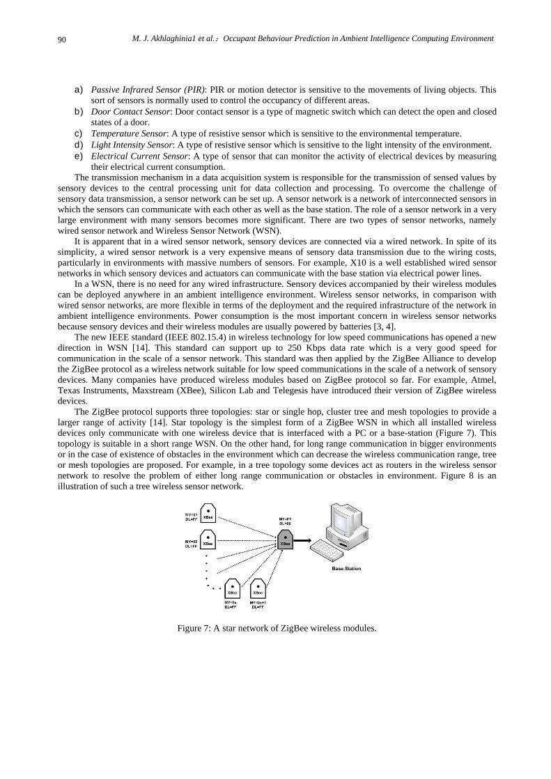
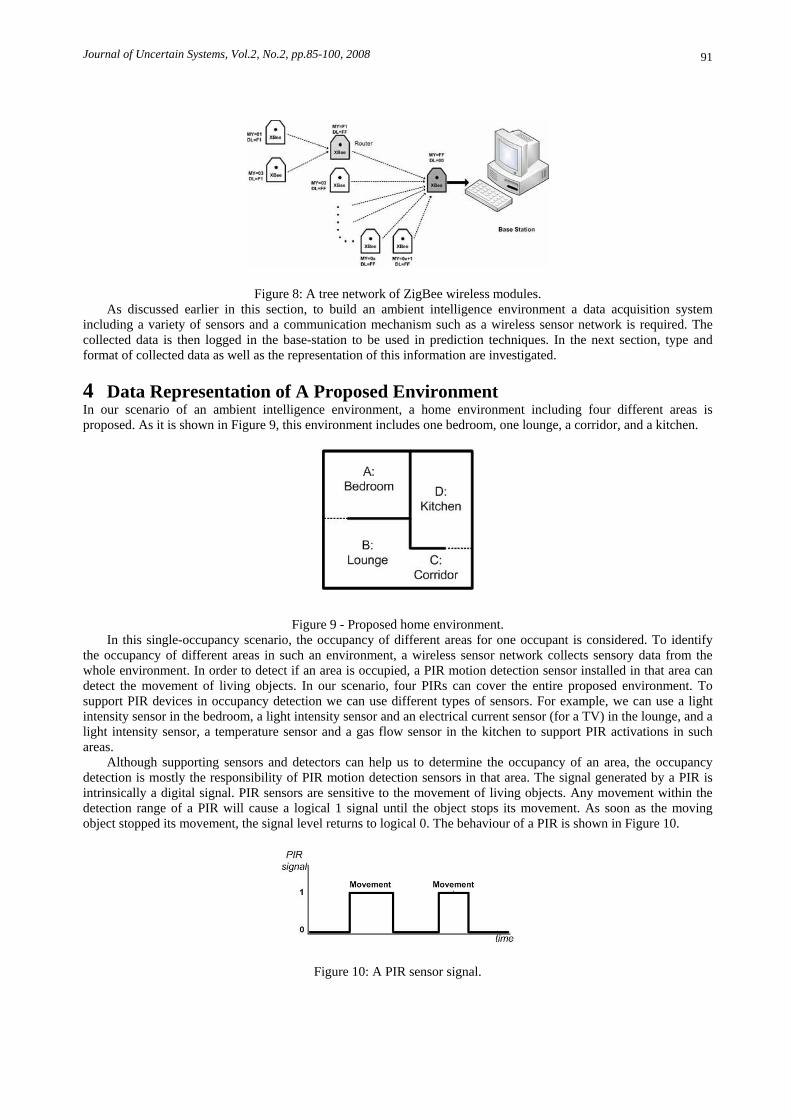
The ZigBee protocol supports three topologies: star or single hop, cluster tree and mesh topologies to provide a larger range of activity [14]. Star topology is the simplest form of a ZigBee WSN in which all installed wireless devices only communicate with one wireless device that is interfaced with a PC or a base-station (Figure 7). This topology is suitable in a short range WSN. On the other hand, for long range communication in bigger environments or in the case of existence of obstacles in the environment which can decrease the wireless communication range, tree or mesh topologies are proposed. For example, in a tree topology some devices act as routers in the wireless sensor network to resolve the problem of either long range communication or obstacles in environment. Figure 8 is an illustration of such a tree wireless sensor network.

Figure 7: A star network of ZigBee wireless modules.


Figure 8: A tree network of ZigBee wireless modules. As discussed earlier in this section, to build an ambient intelligence environment a data acquisition system

including a variety of sensors and a communication mechanism such as a wireless sensor network is required. The collected data is then logged in the base-station to be used in prediction techniques. In the next section, type and format of collected data as well as the representation of this information are investigated.

4 Data Representation of A Proposed Environment In our scenario of an ambient intelligence environment, a home environment including four different areas is proposed. As it is shown in Figure 9, this environment includes one bedroom, one lounge, a corridor, and a kitchen.

Figure 9 - Proposed home environment. In this single-occupancy scenario, the occupancy of different areas for one occupant is considered. To identify

the occupancy of different areas in such an environment, a wireless sensor network collects sensory data from the whole environment. In order to detect if an area is occupied, a PIR motion detection sensor installed in that area can detect the movement of living objects. In our scenario, four PIRs can cover the entire proposed environment. To support PIR devices in occupancy detection we can use different types of sensors. For example, we can use a light intensity sensor in the bedroom, a light intensity sensor and an electrical current sensor (for a TV) in the lounge, and a light intensity sensor, a temperature sensor and a gas flow sensor in the kitchen to support PIR activations in such areas.

Although supporting sensors and detectors can help us to determine the occupancy of an area, the occupancy detection is mostly the responsibility of PIR motion detection sensors in that area. The signal generated by a PIR is intrinsically a digital signal. PIR sensors are sensitive to the movement of living objects. Any movement within the detection range of a PIR will cause a logical 1 signal until the object stops its movement. As soon as the moving object stopped its movement, the signal level returns to logical 0. The behaviour of a PIR is shown in Figure 10.

Figure 10: A PIR sensor signal.


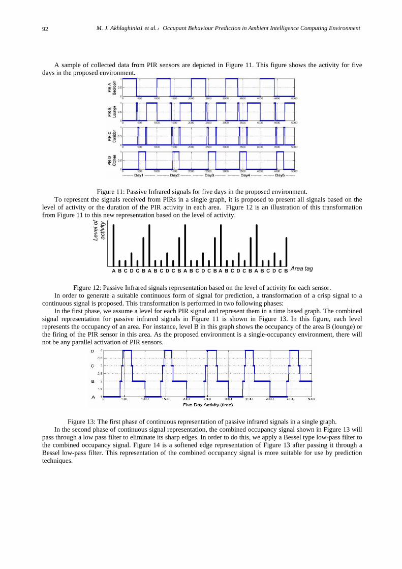
A sample of collected data from PIR sensors are depicted in Figure 11. This figure shows the activity for five days in the proposed environment.

Figure 11: Passive Infrared signals for five days in the proposed environment. To represent the signals received from PIRs in a single graph, it is proposed to present all signals based on the

level of activity or the duration of the PIR activity in each area. Figure 12 is an illustration of this transformation from Figure 11 to this new representation based on the level of activity.

Figure 12: Passive Infrared signals representation based on the level of activity for each sensor. In order to generate a suitable continuous form of signal for prediction, a transformation of a crisp signal to a

continuous signal is proposed. This transformation is performed in two following phases: In the first phase, we assume a level for each PIR signal and represent them in a time based graph. The combined

signal representation for passive infrared signals in Figure 11 is shown in Figure 13. In this figure, each level represents the occupancy of an area. For instance, level B in this graph shows the occupancy of the area B (lounge) or the firing of the PIR sensor in this area. As the proposed environment is a single-occupancy environment, there will not be any parallel activation of PIR sensors.

Figure 13: The first phase of continuous representation of passive infrared signals in a single graph. In the second phase of continuous signal representation, the combined occupancy signal shown in Figure 13 will

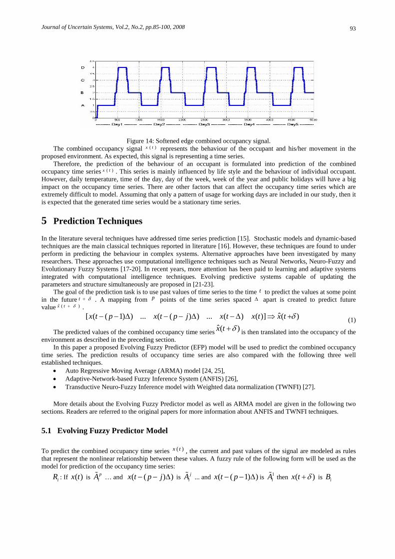
pass through a low pass filter to eliminate its sharp edges. In order to do this, we apply a Bessel type low-pass filter to the combined occupancy signal. Figure 14 is a softened edge representation of Figure 13 after passing it through a Bessel low-pass filter. This representation of the combined occupancy signal is more suitable for use by prediction techniques.


Figure 14: Softened edge combined occupancy signal. The combined occupancy signal represents the behaviour of the occupant and his/her movement in the

proposed environment. As expected, this signal is representing a time series. ( )x t

Therefore, the prediction of the behaviour of an occupant is formulated into prediction of the combined occupancy time series . This series is mainly influenced by life style and the behaviour of individual occupant. However, daily temperature, time of the day, day of the week, week of the year and public holidays will have a big impact on the occupancy time series. There are other factors that can affect the occupancy time series which are extremely difficult to model. Assuming that only a pattern of usage for working days are included in our study, then it is expected that the generated time series would be a stationary time series.

( )x t

5 Prediction Techniques In the literature several techniques have addressed time series prediction [15]. Stochastic models and dynamic-based techniques are the main classical techniques reported in literature [16]. However, these techniques are found to under perform in predicting the behaviour in complex systems. Alternative approaches have been investigated by many researchers. These approaches use computational intelligence techniques such as Neural Networks, Neuro-Fuzzy and Evolutionary Fuzzy Systems [17-20]. In recent years, more attention has been paid to learning and adaptive systems integrated with computational intelligence techniques. Evolving predictive systems capable of updating the parameters and structure simultaneously are proposed in [21-23].

The goal of the prediction task is to use past values of time series to the time t to predict the values at some point in the future t δ+ . A mapping from p points of the time series spaced Δ apart is created to predict future value ˆ ( )x t δ+ .

ˆ[ ( ( 1) ) ... ( ( ) ) ... ( ) ( )] ( )x t p x t p j x t x t x t δ− − Δ − − Δ −Δ ⇒ + (1)

The predicted values of the combined occupancy time series ˆ(x t )δ+ is then translated into the occupancy of the environment as described in the preceding section.

In this paper a proposed Evolving Fuzzy Predictor (EFP) model will be used to predict the combined occupancy time series. The prediction results of occupancy time series are also compared with the following three well established techniques.

• Auto Regressive Moving Average (ARMA) model [24, 25], • Adaptive-Network-based Fuzzy Inference System (ANFIS) [26], • Transductive Neuro-Fuzzy Inference model with Weighted data normalization (TWNFI) [27].

More details about the Evolving Fuzzy Predictor model as well as ARMA model are given in the following two sections. Readers are referred to the original papers for more information about ANFIS and TWNFI techniques.

5.1 Evolving Fuzzy Predictor Model To predict the combined occupancy time series ( )x t , the current and past values of the signal are modeled as rules that represent the nonlinear relationship between these values. A fuzzy rule of the following form will be used as the model for prediction of the occupancy time series:

iR : If ( )x t is piA … and ( ( ) )x t p j− − Δ is j

iA ... and ( ( 1) )x t p− − Δ is 1iA then ( )x t δ+ is iB


where iR is the label of i th rule, ( ( ) ) : = 1, ,x t p j j− − Δ … p is the j th input, (x t )δ+ is the output,

( and ) is a fuzzy label, and

jiA

= 1,2, ,i n… = 1, ,j … p iB is either a real number or a linear combination of inputs

. and 0 1= * ( ) * ( ( 1)i i i piB q q x t q x t p+ + + − −… n)Δ p are the numbers of rules and individual inputs respectively. It is assumed that the universe of input variables is limited to a specific domain interval, i.e.

( ) [ , ]x t x x− +∈ .

The decision, ˆ (x t )δ+ for the th instance, as a function of inputs i ( ( ) ) : = 1 , ,x t p j j p− − Δ … , is given in the following equation:

=1

=1

ˆ ( ) =

n

i ii

n

ii

w Bx t

wδ+

∑

∑ (2)

where iB is the consequent parameters and is the rule firing strength given by: iw

(3) =1

= ( ( ( ) ) = 1, 2,p

i jAij

w x t p j iμ − − Δ∏ …, n

where jAiμ is the membership function (MF) of the fuzzy value . Gaussian membership functions with two

parameters

jiA

jiρ and j

iσ as the mean and spread of MFs are considered.

2

( ( ) )( ( ( ) )) = expj

ij jAi i

x t p jx t p j ρμσ

⎛ ⎞⎛ ⎞− − Δ −⎜ ⎟− − Δ −⎜⎜ ⎟⎝ ⎠⎝ ⎠⎟

)

. (4)

In short, the parameters of a fuzzy rule-based system are defined as . = [ , , ]j ji j i i iBσ ρΘ

The prediction problem is now in the form of identifying the parameters of the rule base, . Starting from the initial values of the parameters, to update these parameters as more data is available, the adaptation technique presented in the next section can be employed.

i jΘ

5.1.1 Predictor Model Adaptation To minimize the difference between the predicted occupancy time series ˆ (x t δ+ and actual occupancy time series

(x t )δ+ , the error generated from all data must be minimized. The following mean square error function is considered for minimization of the prediction error.

2

=1 =1

1 1 ˆ( ) = ( ) = ( ( ) ( ))2 2

s s

k ijk k

E e x t x t 2δ δΘ Θ + − +∑ ∑ (5)

where is the difference between the actual value,ke (x t )δ+ , and the predicted value, ˆ(x t )δ+ , for the k th training data sample. We assume that there are a total of samples in the training data set. s

All parameters of the fuzzy predictor model, = [ , , ]j ji j i i iBσ ρΘ , can be updated using a steepest gradient

descent method to minimize the error function ( )E Θ given in expression (5). The parameters then will be updated by the following rule:

| |ij new ij old ijeηΘ = Θ − ∇ (6)

where is the gradient of parameters and ije∇ η is the rate of descent which may be chosen arbitrarily. The partial derivative of the error function, ( )E Θ with respect to each parameter is given below:

=ij j ji i i

E E EeBσ ρ

⎡ ⎤∂ ∂ ∂∇ ⎢ ⎥∂ ∂ ∂⎣ ⎦

(7)


where

1

k in

i ii

e wEB w

=

∂= −

∂ ∑ (8)

( )

( )

2

1

( ( ) )2 ( )

( ( ) )

ji

k i i jinj j

i i ii

x t p je w B x tE

x t p j w

ρδσ

ρ ρ=

⎛ ⎞− − Δ −− + ⎜ ⎟

∂ ⎝= −∂ − − Δ − ∑

⎠ (9)

( )

2

1

( ( ) )2 ( )j

ik i i j

inj j

i i ii

x t p je w B x tE

w

ρδσ

σ σ=

⎛ ⎞− − Δ −− + ⎜ ⎟

∂ ⎝= −∂ ∑

⎠

T

(10)

It is anticipated that when the parameters are adapted, the prediction error will be reduced. It should be noted that the gradient descent technique mentioned above suffers from various convergence problems. This has been investigated by many researchers. The convergence problem of the steepest descent technique in fuzzy inference systems modelling is discussed in [28].

It is reasonable to take large steps down the gradient at locations where the gradient is small and small steps where the gradient is large. If both gradient and curvature information namely the second derivatives are used then the error will be minimized in shorter time and more accurately.

The gradient descent is too slow for real-time adaptation. To increase the speed, the Levenberg-Marquardt (LM) algorithm is considered for parameters adaptation [29]. This algorithm is designed to approach second-order training speed without having to compute the Hessian matrix. The LM algorithm update rule is given as:

1| | ( )Tij new ij old kJ J I J eμ −Θ = Θ − + (11)

where 0μ ≥ , and ijJ e= ∇ I is the identity matrix. Even though this technique is computationally more demanding, it will update the parameters of the fuzzy rule-base more quickly. This has proven to be a useful tool for real-time rule adaptation.

5.2 Auto Regressive Moving Average This technique is used as a basis for the analysis and it is a well established technique in prediction of financial time series. Any ARMA model has two parameters respectively, p and . The first parameter is the Auto Regression

parameter and the second parameter is the Moving Average parameter. Hence an ARMA process

q

( )x t can be presented as follows [25]:

1 1( ) ( 1) ... ( ) ( ) ( 1) ... ( )p qx t x t x t p z t z t z t qφ φ θ θ− − − − − = + − + + − (12)

where is the white noise with mean 0 and variance( )z t 2σ , φ is the coefficient of the Auto Regression part, and θ

is the coefficient of the Moving Average part. Expression (12) can be formulated as:

1 1( ) ( ) ( ) ( )

p q

i ii i

x t z t x t i z t iφ θ= =

= + − + −∑ ∑ (13)

The polynomials φ and θ will be referred to as the autoregressive and moving average polynomials

respectively. Applying the Innovations Algorithm Proposition [25] to the transformed process, ( )x t , we obtain:

1

11

( 1) ( ( 1 ) ( 1 ) ) 1

( 1) ( ) . . . ( 1 ) ( ( 1 ) ( 1 ) )

m a x ( , )

t

t jj

q

p t jj

x t x t j x t j

x t x t x t p x t j x t j t m

m p q

θ

ϕ ϕ θ

∧ ∧

=

∧ ∧

=

⎧+ = + − − + − ≤ <⎪

⎪⎨⎪ + = + + + − + + − − + − ≥⎪⎩

=

∑

∑

t m (14)


Equations (14) determine the one-step predictors ( 2 )x∧

, ( 3 )x∧

, … recursively.

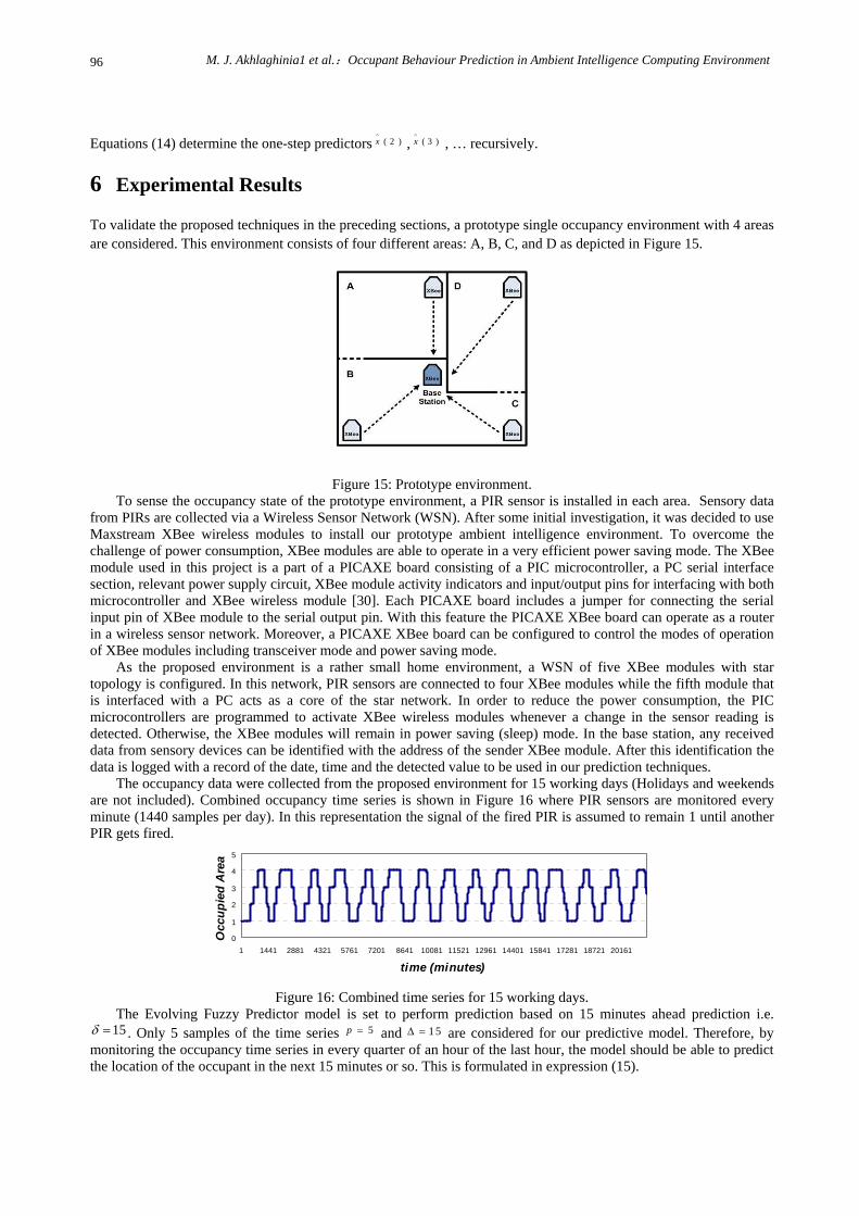
6 Experimental Results To validate the proposed techniques in the preceding sections, a prototype single occupancy environment with 4 areas are considered. This environment consists of four different areas: A, B, C, and D as depicted in Figure 15.

Figure 15: Prototype environment. To sense the occupancy state of the prototype environment, a PIR sensor is installed in each area. Sensory data

from PIRs are collected via a Wireless Sensor Network (WSN). After some initial investigation, it was decided to use Maxstream XBee wireless modules to install our prototype ambient intelligence environment. To overcome the challenge of power consumption, XBee modules are able to operate in a very efficient power saving mode. The XBee module used in this project is a part of a PICAXE board consisting of a PIC microcontroller, a PC serial interface section, relevant power supply circuit, XBee module activity indicators and input/output pins for interfacing with both microcontroller and XBee wireless module [30]. Each PICAXE board includes a jumper for connecting the serial input pin of XBee module to the serial output pin. With this feature the PICAXE XBee board can operate as a router in a wireless sensor network. Moreover, a PICAXE XBee board can be configured to control the modes of operation of XBee modules including transceiver mode and power saving mode.

As the proposed environment is a rather small home environment, a WSN of five XBee modules with star topology is configured. In this network, PIR sensors are connected to four XBee modules while the fifth module that is interfaced with a PC acts as a core of the star network. In order to reduce the power consumption, the PIC microcontrollers are programmed to activate XBee wireless modules whenever a change in the sensor reading is detected. Otherwise, the XBee modules will remain in power saving (sleep) mode. In the base station, any received data from sensory devices can be identified with the address of the sender XBee module. After this identification the data is logged with a record of the date, time and the detected value to be used in our prediction techniques.

The occupancy data were collected from the proposed environment for 15 working days (Holidays and weekends are not included). Combined occupancy time series is shown in Figure 16 where PIR sensors are monitored every minute (1440 samples per day). In this representation the signal of the fired PIR is assumed to remain 1 until another PIR gets fired.

0

1

2

3

4

5

1 1441 2881 4321 5761 7201 8641 10081 11521 12961 14401 15841 17281 18721 20161

time (minutes)

Occ

upie

d A

rea

Figure 16: Combined time series for 15 working days.

The Evolving Fuzzy Predictor model is set to perform prediction based on 15 minutes ahead prediction i.e. 15δ = . Only 5 samples of the time series 5p = and 15Δ = are considered for our predictive model. Therefore, by

monitoring the occupancy time series in every quarter of an hour of the last hour, the model should be able to predict the location of the occupant in the next 15 minutes or so. This is formulated in expression (15).


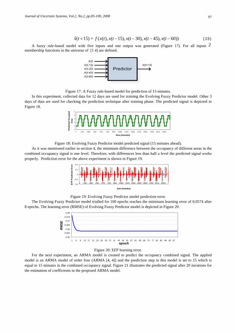
(15) ˆ( 15) = ( ( ), ( 15), ( 30), ( 45), ( 60))x t f x t x t x t x t x t+ − − − −A fuzzy rule-based model with five inputs and one output was generated (Figure 17). For all inputs 2

membership functions in the universe of [1 4] are defined.

Figure 17: A Fuzzy rule-based model for prediction of 15 minutes. In this experiment, collected data for 12 days are used for training the Evolving Fuzzy Predictor model. Other 3

days of data are used for checking the prediction technique after training phase. The predicted signal is depicted in Figure 18.

0

1

2

3

4

5

1 1441 2881 4321 5761 7201 8641 10081 11521 12961 14401 15841 17281 18721 20161

time (minutes)

Pred

icte

d O

ccup

ied

Are

a

Figure 18: Evolving Fuzzy Predictor model predicted signal (15 minutes ahead).

As it was mentioned earlier in section 4, the minimum difference between the occupancy of different areas in the combined occupancy signal is one level. Therefore, with differences less than half a level the predicted signal works properly. Prediction error for the above experiment is shown in Figure 19.

-0.4

-0.2

0

0.2

0.4

1 1441 2881 4321 5761 7201 8641 10081 11521 12961 14401 15841 17281 18721 20161

time (minutes)

EFP

Pre

dict

ion

Err

or

Figure 19: Evolving Fuzzy Predictor model prediction error.

The Evolving Fuzzy Predictor model trialled for 100 epochs reaches the minimum learning error of 0.0574 after 8 epochs. The learning error (RMSE) of Evolving Fuzzy Predictor model is depicted in Figure 20.

0.05

0.055

0.06

0.065

0.07

0.075

0.08

1 5 9 13 17 21 25 29 33 37 41 45 49 53 57 61 65 69 73 77 81 85 89 93 97epoch

RM

SE

Figure 20: EFP learning error.

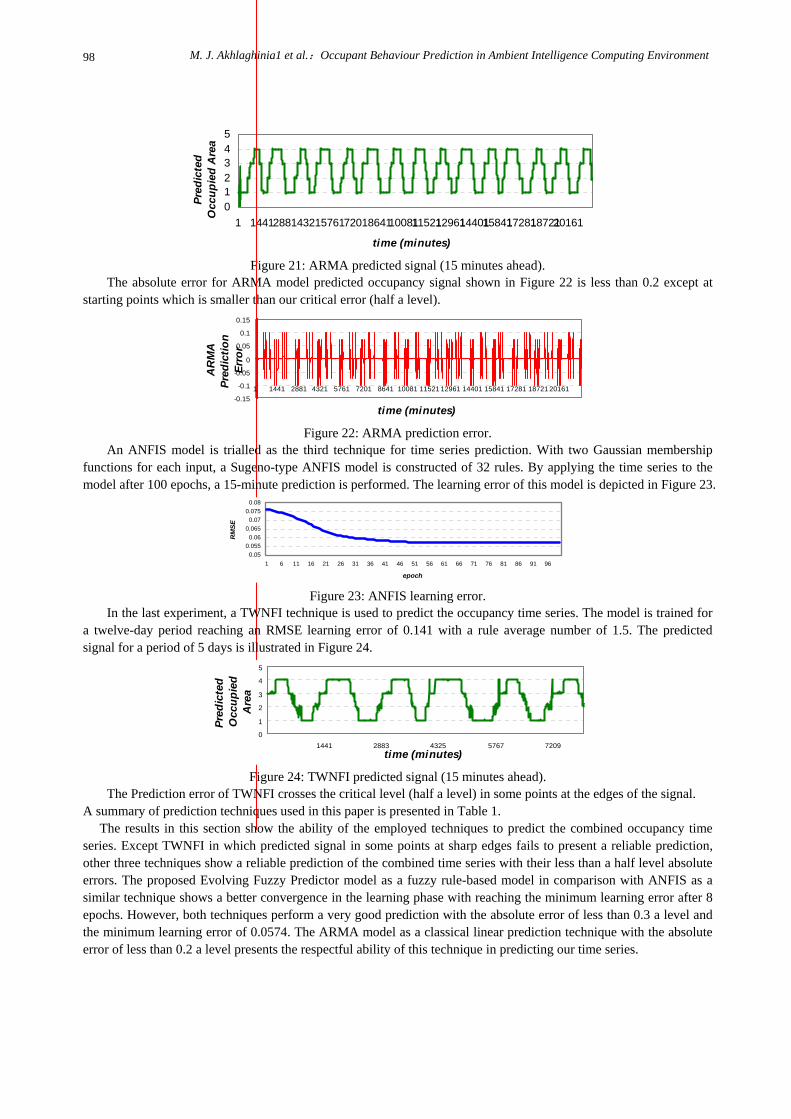
For the next experiment, an ARMA model is created to predict the occupancy combined signal. The applied model is an ARMA model of order four (ARMA [4, 4]) and the prediction step in this model is set to 15 which is equal to 15 minutes in the combined occupancy signal. Figure 21 illustrates the predicted signal after 20 iterations for the estimation of coefficients in the proposed ARMA model.


012345

1 1441288143215761720186411008111521129611440115841172811872120161

time (minutes)

Pred

icte

dO

ccup

ied

Are

a

Figure 21: ARMA predicted signal (15 minutes ahead).

The absolute error for ARMA model predicted occupancy signal shown in Figure 22 is less than 0.2 except at starting points which is smaller than our critical error (half a level).

-0.15

-0.1

-0.05

0

0.05

0.1

0.15

1 1441 2881 4321 5761 7201 8641 10081 11521 12961 14401 15841 17281 18721 20161

time (minutes)

AR

MA

Pred

ictio

nEr

ror

Figure 22: ARMA prediction error.

An ANFIS model is trialled as the third technique for time series prediction. With two Gaussian membership functions for each input, a Sugeno-type ANFIS model is constructed of 32 rules. By applying the time series to the model after 100 epochs, a 15-minute prediction is performed. The learning error of this model is depicted in Figure 23.

0.050.0550.06

0.0650.07

0.0750.08

1 6 11 16 21 26 31 36 41 46 51 56 61 66 71 76 81 86 91 96

epoch

RM

SE

Figure 23: ANFIS learning error.

In the last experiment, a TWNFI technique is used to predict the occupancy time series. The model is trained for a twelve-day period reaching an RMSE learning error of 0.141 with a rule average number of 1.5. The predicted signal for a period of 5 days is illustrated in Figure 24.

0

1

2

3

4

5

1441 2883 4325 5767 7209time (minutes)

Pred

icte

dO

ccup

ied

Are

a

Figure 24: TWNFI predicted signal (15 minutes ahead).

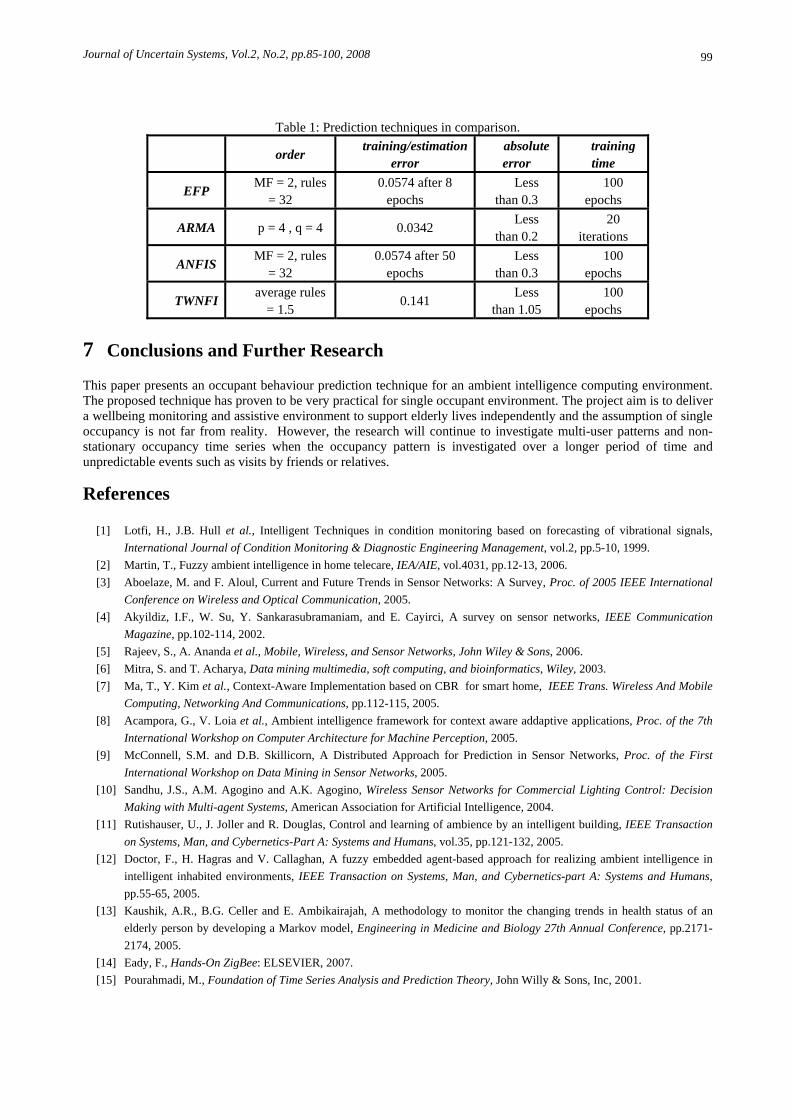
The Prediction error of TWNFI crosses the critical level (half a level) in some points at the edges of the signal. A summary of prediction techniques used in this paper is presented in Table 1. The results in this section show the ability of the employed techniques to predict the combined occupancy time series. Except TWNFI in which predicted signal in some points at sharp edges fails to present a reliable prediction, other three techniques show a reliable prediction of the combined time series with their less than a half level absolute errors. The proposed Evolving Fuzzy Predictor model as a fuzzy rule-based model in comparison with ANFIS as a similar technique shows a better convergence in the learning phase with reaching the minimum learning error after 8 epochs. However, both techniques perform a very good prediction with the absolute error of less than 0.3 a level and the minimum learning error of 0.0574. The ARMA model as a classical linear prediction technique with the absolute error of less than 0.2 a level presents the respectful ability of this technique in predicting our time series.


Table 1: Prediction techniques in comparison.

order training/estimation error

absolute error

training time

EFP MF = 2, rules = 32

0.0574 after 8 epochs

Less than 0.3

100 epochs

ARMA p = 4 , q = 4 0.0342 Less than 0.2

20 iterations

ANFIS MF = 2, rules = 32

0.0574 after 50 epochs

Less than 0.3

100 epochs

TWNFI average rules = 1.5 0.141 Less

than 1.05 100

epochs

7 Conclusions and Further Research This paper presents an occupant behaviour prediction technique for an ambient intelligence computing environment. The proposed technique has proven to be very practical for single occupant environment. The project aim is to deliver a wellbeing monitoring and assistive environment to support elderly lives independently and the assumption of single occupancy is not far from reality. However, the research will continue to investigate multi-user patterns and non-stationary occupancy time series when the occupancy pattern is investigated over a longer period of time and unpredictable events such as visits by friends or relatives.

References

[1] Lotfi, H., J.B. Hull et al., Intelligent Techniques in condition monitoring based on forecasting of vibrational signals, International Journal of Condition Monitoring & Diagnostic Engineering Management, vol.2, pp.5-10, 1999.

[2] Martin, T., Fuzzy ambient intelligence in home telecare, IEA/AIE, vol.4031, pp.12-13, 2006. [3] Aboelaze, M. and F. Aloul, Current and Future Trends in Sensor Networks: A Survey, Proc. of 2005 IEEE International

Conference on Wireless and Optical Communication, 2005. [4] Akyildiz, I.F., W. Su, Y. Sankarasubramaniam, and E. Cayirci, A survey on sensor networks, IEEE Communication

Magazine, pp.102-114, 2002. [5] Rajeev, S., A. Ananda et al., Mobile, Wireless, and Sensor Networks, John Wiley & Sons, 2006. [6] Mitra, S. and T. Acharya, Data mining multimedia, soft computing, and bioinformatics, Wiley, 2003. [7] Ma, T., Y. Kim et al., Context-Aware Implementation based on CBR for smart home, IEEE Trans. Wireless And Mobile

Computing, Networking And Communications, pp.112-115, 2005. [8] Acampora, G., V. Loia et al., Ambient intelligence framework for context aware addaptive applications, Proc. of the 7th

International Workshop on Computer Architecture for Machine Perception, 2005. [9] McConnell, S.M. and D.B. Skillicorn, A Distributed Approach for Prediction in Sensor Networks, Proc. of the First

International Workshop on Data Mining in Sensor Networks, 2005. [10] Sandhu, J.S., A.M. Agogino and A.K. Agogino, Wireless Sensor Networks for Commercial Lighting Control: Decision

Making with Multi-agent Systems, American Association for Artificial Intelligence, 2004. [11] Rutishauser, U., J. Joller and R. Douglas, Control and learning of ambience by an intelligent building, IEEE Transaction

on Systems, Man, and Cybernetics-Part A: Systems and Humans, vol.35, pp.121-132, 2005. [12] Doctor, F., H. Hagras and V. Callaghan, A fuzzy embedded agent-based approach for realizing ambient intelligence in

intelligent inhabited environments, IEEE Transaction on Systems, Man, and Cybernetics-part A: Systems and Humans, pp.55-65, 2005.

[13] Kaushik, A.R., B.G. Celler and E. Ambikairajah, A methodology to monitor the changing trends in health status of an elderly person by developing a Markov model, Engineering in Medicine and Biology 27th Annual Conference, pp.2171-2174, 2005.

[14] Eady, F., Hands-On ZigBee: ELSEVIER, 2007. [15] Pourahmadi, M., Foundation of Time Series Analysis and Prediction Theory, John Willy & Sons, Inc, 2001.


[16] Armstrong, J.S., Principles of forecasting: a handbook for researchers and practitioner, Norwell, Massachusetts, Kluwer Academic Publishers, 2001.

[17] Acampora, G. and V. Loia, Using fuzzy technology in ambient intelligence environment, Proc. of IEEE International Conference on Fuzzy Systems, FUZZ-IEEE2005 Reno, NV, United States, 2005.

[18] Figueiredo, M., R. Ballini et al., Learning algorithms for a class of neuro-fuzzy network and applications, IEEE Transactions on Systems, Man, and Cybernetics – Part C: Applications and Review, vol.34, pp.293-301, 2004.

[19] Ishibuchi, H. and T. Yamamoto, Rule weight specification in fuzzy rule-based classification systems, IEEE Transactions on Fuzzy Systems, vol.13, pp.428-435, 2005.

[20] Liang, Y. and X. Liang, Improving signal prediction performance of neural networks through multi-resolution learning approach, IEEE Transactions on Systems, Man, and Cybernetics-Part B: Cybernetics, vol.36, pp.341-352, 2006.

[21] Angelov, P., Evolving Rule Based Models: A Tool for Design of Flexible Adaptive Systems, Physical-Verlag, Heidelberg, 2002.

[22] Chen, Y.M. and C.-T. Lin, Dynamic parameter optimization of evolutionary computation for on-line prediction of time series with changing dynamics, Applied Soft Computing Journal-Soft Computing for Time Series Prediction, vol.7, pp.1170-1176, 2007.

[23] Kasabov, N. and Q. Song, DENFIS: dynamic evolving neural-fuzzy inference system and its application for time-series prediction, IEEE Transactions on Fuzzy Systems, vol.10, pp.144-154, 2002.

[24] Makhoul, J., Linear prediction: A tutorial review, IEEE, pp.561-580, 1975 [25] Brockwell, P. J. and R. A. Davis, Time Series: Theory and Methods, Springer-Verlag, 1987. [26] Jang, J.-S.R., C.-T. Sun and E. Mizutani, Neuro-Fuzzy and Soft Computing: a computational approach to learning and

machine intelligence, Prentice-Hall, 1996. [27] Song, Q. and N. Kasabov, TWNFI-a transductive neuro-fuzzy inference system with weighted data normalization for

personalized modeling, Neural Networks, vol.19, pp.1591-1596, 2006. [28] Wang, J.-S. and G. Lee, Selft-Adaptive Neuro-Fuzzy Inference Systems for Classification Applications, IEEE Transactions

on Fuzzy Systems, vol.10, 2002. [29] Miller, R. E., Optimization: Foundations and Application, Wiley-Interscience, 1999. [30] PICAXE and Xbee, Tutorial, Revolution Education Ltd., 2006.

Documents

Occupant Behaviour Prediction in Ambient … M. J. Akhlaghinia1 et al.：Occupant Behaviour Prediction in Ambient Intelligence Computing Environment the main focus of this article,