Occurrence and Movement of Groundwater

8/4/2019 Occurrence and Movement of Groundwater

http://slidepdf.com/reader/full/occurrence-and-movement-of-groundwater 1/18

Snow

Infiltration

Precipitation

Water table

Lake

Spring

Surface

Transpiration

Evaporation

Condensation

Groundwater

RiverOcean

runoff

EM 1110-2-142128 Feb 99

2-1

Figure 2-1. Hydrologic cycle

Chapter 2

Occurrence and Movement of Groundwater

2-1. General

The occurrence and movement of groundwater are

related to physical forces acting in the subsurface and

the geologic environment in which they occur. This

chapter presents a general overview of basic concepts

which explain and quantify these forces and

environments as related to groundwater. For Corps-

specific applications, a section on estimating capture

zones of pumping wells is included. Additionally, a

discussion on saltwater intrusion is included. For a

more detailed understanding of general groundwater

concepts, the reader is referred to Fetter (1994).

2-2. Hydrologic Cycle

a. The Earth's hydrologic cycle consists of many

varied and interacting processes involving all three

phases of water. A schematic diagram of the flow of

water from the atmosphere, to the surface and

subsurface, and eventually back to the atmosphere is

shown in Figure 2-1.

b. Groundwater flow is but one part of this com-

plex dynamic hydrologic cycle. Saturated formations

below the surface act as mediums for the transmission

of groundwater, and as reservoirs for the storage of

water. Water infiltrates to these formations from the

surface and is transmitted slowly for varying distances

until it returns to the surface by action of natural flow,

vegetation, or man (Todd 1964). Groundwater is the

largest source of available water within the United

States, accounting for 97 percent of the available fresh

water in the United States, and 23 percent of fresh-

water usage (Solley and Pierce 1992).

2-3. Subsurface Distribution

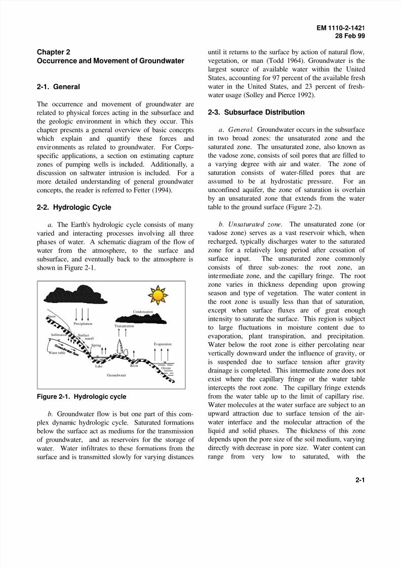
a. General. Groundwater occurs in the subsurface

in two broad zones: the unsaturated zone and the

saturated zone. The unsaturated zone, also known as

the vadose zone, consists of soil pores that are filled to

a varying degree with air and water. The zone of

saturation consists of water-filled pores that are

assumed to be at hydrostatic pressure. For an

unconfined aquifer, the zone of saturation is overlain

by an unsaturated zone that extends from the watertable to the ground surface (Figure 2-2).

b. Unsaturated zone. The unsaturated zone (or

vadose zone) serves as a vast reservoir which, when

recharged, typically discharges water to the saturated

zone for a relatively long period after cessation of

surface input. The unsaturated zone commonly

consists of three sub-zones: the root zone, an

intermediate zone, and the capillary fringe. The root

zone varies in thickness depending upon growing

season and type of vegetation. The water content in

the root zone is usually less than that of saturation,

except when surface fluxes are of great enough

intensity to saturate the surface. This region is subject

to large fluctuations in moisture content due to

evaporation, plant transpiration, and precipitation.

Water below the root zone is either percolating near

vertically downward under the influence of gravity, or

is suspended due to surface tension after gravity

drainage is completed. This intermediate zone does not

exist where the capillary fringe or the water table

intercepts the root zone. The capillary fringe extends

from the water table up to the limit of capillary rise.Water molecules at the water surface are subject to an

upward attraction due to surface tension of the air-

water interface and the molecular attraction of the

liquid and solid phases. The thickness of this zone

depends upon the pore size of the soil medium, varying

directly with decrease in pore size. Water content can

range from very low to saturated, with the



h ' z% p

Dg%

v 2

2g

EM 1110-2-142128 Feb 99

2-2

Figure 2-2. Subsurface distribution of water

lower part of the capillary fringe often being saturated. groundwater flows through interconnected voids in

Infiltration and flow in the unsaturated zone are response to the difference in fluid pressure and

discussed in Section 6-3. elevation. The driving force is measured in terms of

c. Saturated zone. In the zone of saturation, all head) is defined by Bernoulli's equation:communicating voids are filled with water under

hydrostatic pressure. Water in the saturated zone is

known as groundwater or phreatic water.

2-4. Forces Acting on Groundwater

External forces which act on water in the subsurface

include gravity, pressure from the atmosphere and

overlying water, and molecular attraction between

solids and water. In the subsurface, water can occur in

the following: as water vapor which moves fromregions of higher pressure to lower pressure, as

condensed water which is absorbed by dry soil

particles, as water which is retained on particles under

the molecular force of adhesion, and as water which is

not subject to attractive forces towards the surface of

solid particles and is under the influence of

gravitational forces. In the saturated zone,

hydraulic head. Hydraulic head (or potentiometric

(2-1)

where

h = hydraulic head

z = elevation above datum

p = fluid pressure with constant density D

g = acceleration due to gravity

v = fluid velocity

Pressure head (or fluid pressure) h is defined as: p



h p

' p

Dg

h ' z%h p

EM 1110-2-142128 Feb 99

2-3

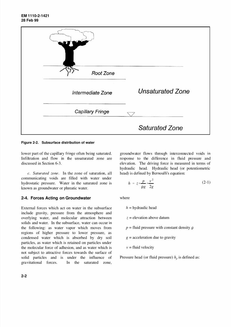
Figure 2-3. Relationship between hydraulic head,pressure head, and elevation head within a well

(2-2)

By convention, pressure head is expressed in units

above atmospheric pressure. In the unsaturated zone,

water is held in tension and pressure head is less thanatmospheric pressure (h < 0). Below the water table, p

in the saturated zone, pressure head is greater than

atmospheric pressure (h > 0). Because groundwater p

velocities are usually very low, the velocity component

of hydraulic head can be neglected. Thus, hydraulic

head can usually be expressed as:

(2-3)

Figure 2-3 depicts Equation 2-3 within a well.

2-5. Water Table

As illustrated by Figure 2-3, the height of water

measured in wells is the sum of elevation head and

pressure head, where the pressure head is equal to theheight of the water column above the screened interval

within the well. Freeze and Cherry (1979) define the

water table as located at the level at which water

stands within a shallow well which penetrates the

surficial deposits just deeply enough to encounter

standing water. Thus, the hydraulic head at the water

table is equal to the elevation head; and the pore water

pressure at the water table is equivalent to atmospheric

pressure.

2-6. Potentiometric Surface

The water table is defined as the surface in a

groundwater body at which the pressure is

atmospheric, and is measured by the level at which

water stands in wells that penetrate the water body just

far enough to hold standing water. The potentiometric

surface approximates the level to which water will rise

in a tightly cased well which can be screened at the

water table or at greater depth. In wells that penetrate

to greater depths within the aquifer, the potentiometric

surface may be above or below the water table

depending on whether an upward or downward

component of flow exists. The potentiometric surface

can vary with the depth of a well. In confined aquifers(Section 2-6), the potentiometric surface will rise

above the aquifer surface. The water table is the

potentiometric surface for an unconfined aquifer

(Section 2-6). Where the head varies appreciably with

depth in an aquifer, a potentiometric surface is

meaningful only if it describes the static head along a

particular specified stratum in that aquifer. The

concept of potentiometric surface is only rigorously

valid for defining horizontal flow directions from

horizontal aquifers.

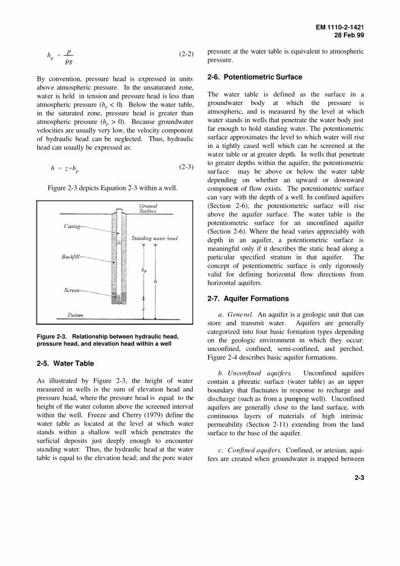
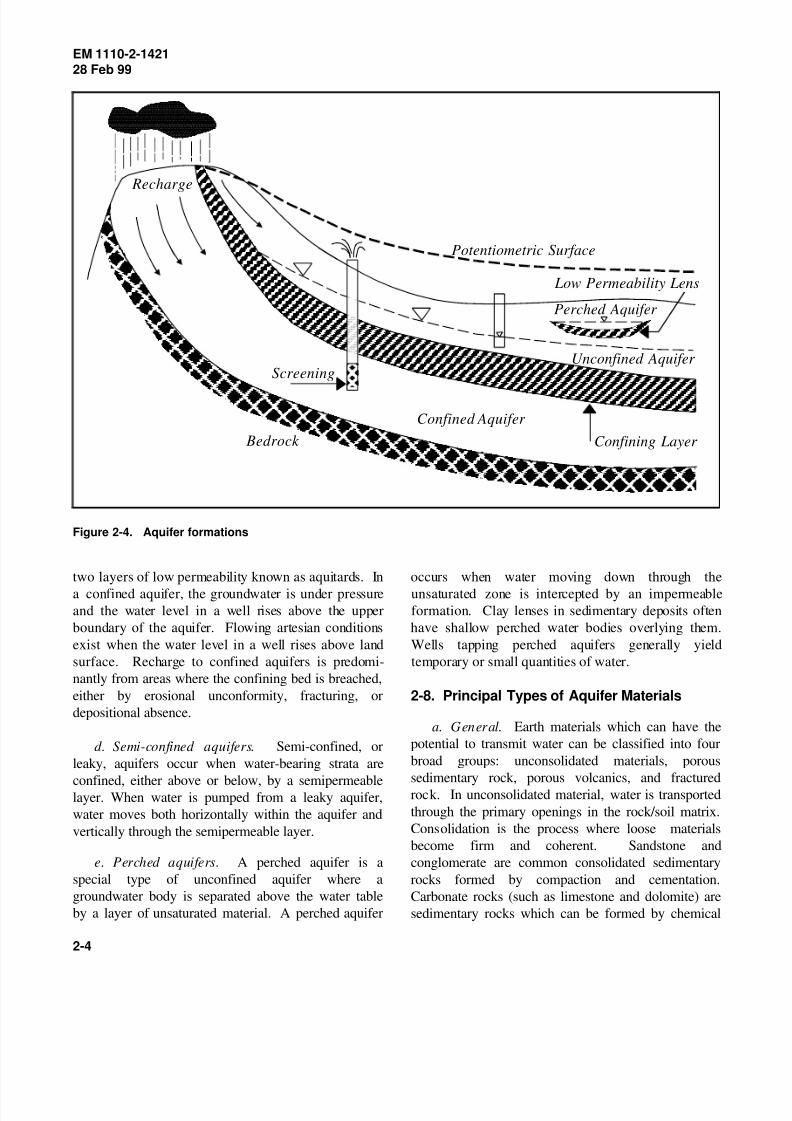
2-7. Aquifer Formations

a. General. An aquifer is a geologic unit that can

store and transmit water. Aquifers are generally

categorized into four basic formation types depending

on the geologic environment in which they occur:

unconfined, confined, semi-confined, and perched.

Figure 2-4 describes basic aquifer formations.

b. Unconfined aquifers. Unconfined aquifers

contain a phreatic surface (water table) as an upper

boundary that fluctuates in response to recharge and

discharge (such as from a pumping well). Unconfinedaquifers are generally close to the land surface, with

continuous layers of materials of high intrinsic

permeability (Section 2-11) extending from the land

surface to the base of the aquifer.

c. Confined aquifers. Confined, or artesian, aqui-

fers are created when groundwater is trapped between



Confined Aquifer

Recharge

Unconfined Aquifer

Potentiometric Surface

Bedrock Confining Layer

Perched Aquifer

Low Permeability Lens

Screening

EM 1110-2-142128 Feb 99

2-4

Figure 2-4. Aquifer formations

two layers of low permeability known as aquitards. In occurs when water moving down through the

a confined aquifer, the groundwater is under pressure unsaturated zone is intercepted by an impermeableand the water level in a well rises above the upper formation. Clay lenses in sedimentary deposits often

boundary of the aquifer. Flowing artesian conditions have shallow perched water bodies overlying them.

exist when the water level in a well rises above land Wells tapping perched aquifers generally yield

surface. Recharge to confined aquifers is predomi- temporary or small quantities of water.

nantly from areas where the confining bed is breached,

either by erosional unconformity, fracturing, or

depositional absence.

d. Semi-confined aquifers. Semi-confined, or

leaky, aquifers occur when water-bearing strata are

confined, either above or below, by a semipermeablelayer. When water is pumped from a leaky aquifer,

water moves both horizontally within the aquifer and

vertically through the semipermeable layer.

e. Perched aquifers. A perched aquifer is a

special type of unconfined aquifer where a

groundwater body is separated above the water table

by a layer of unsaturated material. A perched aquifer

2-8. Principal Types of Aquifer Materials

a. General. Earth materials which can have the

potential to transmit water can be classified into four

broad groups: unconsolidated materials, porous

sedimentary rock, porous volcanics, and fractured

rock. In unconsolidated material, water is transported

through the primary openings in the rock/soil matrix.

Consolidation is the process where loose materials

become firm and coherent. Sandstone and

conglomerate are common consolidated sedimentary

rocks formed by compaction and cementation.

Carbonate rocks (such as limestone and dolomite) are

sedimentary rocks which can be formed by chemical



EM 1110-2-142128 Feb 99

2-5

precipitation. Water is usually transported through common sequence in the southern United States.

secondary openings in carbonate rocks enlarged by the Additionally, coral reefs, shells, and other calcite-rich

dissolution of rock by water. The movement of water deposits commonly occur in areas with temperate

through volcanics and fractured rock is dependent upon climatic conditions.

the interconnectedness and frequency of flow

pathways. (4) Eolian deposits. Materials which are

b. Gravel and sand. Gravel and sand aquifers are The sorting action of the wind tends to produce

the source of most water pumped in the United States. deposits that are uniform on a local scale, and in some

Gravels and sands originate from alluvial, lacustrine, cases quite uniform over large areas. Eolian deposits

marine, or eolian glacial deposition. consist of silt or sand. Eolian sands occur wherever

(1) Alluvial deposits. Alluvial deposits of peren- comparison with alluvial deposits, eolian sands are

nial streams are usually fairly well sorted and therefore quite homogeneous and are as isotropic (Section 2-13)

permeable. Ephemeral streams typically deposit sand as any deposits occurring in nature. Eolian deposits of

and gravel with much less sorting. Stream channels silt, called loess, are associated with the abnormally

are sensitive to changes in sediment load, gradient, and high wind velocities associated with glacial ice fronts.

velocity. This can result in lateral distribution of Loess occurs in the shallow subsurface in large areasalluvial deposits over large areas. Areas with greater of the Midwest and Great Plains regions of North

streambed slope typically contain coarser deposits. America.

Alluvial fans occur in arid or semiarid regions where a

stream issues from a narrow canyon onto a plain or (5) Glacial deposits. Unlike water and wind,

valley floor. Viewed from above, they have the shape glacial ice can entrain unconsolidated deposits of all

of an open fan, the apex being at the valley mouth. sizes from sediments to boulders. Glacial till is non-

These alluvial deposits are coarsest at the point where sorted, non-stratified sediment deposited beneath, from

the stream exits the canyon mouth, and become finer within, or from the top of glacial ice. Glacial outwash

with increasing distance from the point of initial (or glaciofluvial) deposits consist of coarse-grained

deposition. sediments deposited by meltwater in front of a glacier.

The sorting and homogeneity of glaciofluvial deposits

(2) Lacustrine deposits. The central and lowerportions of alluvium-filled valleys may consist of fine-

grained lacustrine (or lakebed) deposits. When a

stream flows into a lake, the current is abruptly c. Sandstone and conglomerate. Sandstone and

checked. The coarser sediment settles rapidly to the conglomerates are the consolidated equivalents of sand

bottom, while finer materials are transported further and gravel. Consolidation results from compaction and

into the body of relatively still water. Thus, the central cementation. The highest yielding sandstone aquifers

areas of valleys which have received lacustrine occur where partial consolidation takes place. These

deposits often consist of finer-grained, yield water from the pores between grains, although

lower-permeability materials. Lacustrine deposits secondary openings such as fractures and joints can

usually consist of fine-grained materials that are not also serve as channels of flow.

normally considered aquifers.

(3) Marine deposits. Marine deposits originate from calcium, magnesium, or iron, are widespread

from sediment transported to the ocean by rivers and throughout the United States. Limestone and dolomite,

erosion of the ocean floor. As a sea moves inland, which originate from calcium-rich deposits, are the

deposits at a point in the ocean bottom near the shore most common carbonate rocks. Carbonates are

become gradually finer due to uniform wave energy. typically brittle and susceptible to fracturing.

Conversely, as the sea regresses, deposition progresses Fractures and joints in limestone yield water in small to

gradually from finer to coarser deposits. This is a moderate amounts. However, because water acts as a

transported by the wind are known as eolian deposits.

surface sediments are available for transport. In

depend upon environmental conditions and distancefrom the glacial front.

d. Carbonate rocks. Carbonate rocks, formed



n '

V v

V T

EM 1110-2-142128 Feb 99

2-6

weak acid to carbonates, dissolution of rock by water

enlarges openings. The limestones that yield the

highest amount of water are those in which a sizable

portion of the original rock has been dissolved or

removed. These areas are commonly referred to as

karst. Thus, large amounts of flow can potentially be

transmitted in carbonate rocks.

e. Volcanics. Basalt is an important aquifer

material in parts of the western United States, most

notably central Idaho, where enormous flows of lava

have spread out over large areas in successive sheets of

varying thickness. The ability of basalt formations to

transmit water is dependent on the presence of

fractures, cracks, and tubes or caverns, and can be

significant. Near the surface, rapid cooling produces

jointing. Fracturing below the surface occurs as the

crust cools, causing differential flow velocities withdepth. Other volcanic rocks, including rhyolite and

other more siliceous rocks, do not usually yield water

in quantities comparable to those secured from basalt.

Another major source of groundwater in some parts of

the western United States is found in sedimentary

“interbed” materials which occur between basalt flows.

This interbedded material is generally alluvial or

colluvial in nature, consisting of sands, gravels, and

residuum (particularly granite). When the interbedded

materials tend to be finer-grained, the interbed acts as a

confining layer.

f. Fractured rock. Crystalline and metamorphic

rocks, including granite, basic igneous rocks, gneiss,

schist, quartzite, and slate are relatively impermeable.

Water in these areas is supplied as a result of jointing

and fracturing. The yield of water from fractured rock

is dependent upon the frequency and interconnected-

ness of flow pathways.

2-9. Movement of Groundwater

Groundwater moves through the sub-surface fromareas of greater hydraulic head to areas of lower

hydraulic head (Equation 2-3). The rate of

groundwater movement depends upon the slope of the

hydraulic head (hydraulic gradient), and intrinsic

aquifer and fluid properties.

2-10. Porosity and Specific Yield

a. Porosity. Porosity n is defined as the ratio of

void space to the total volume of media:

(2-4)

where

V = volume of void space [L ]v3

V = total volume (volume of solids plus volumeT

of voids) [L ]3

In unconsolidated materials, porosity is principally

governed by three properties of the media: grain

packing, grain shape, and grain size distribution. The

effect of packing may be observed in two-dimensional

models comprised of spherical, uniform-sized balls.

Arranging the balls in a cubic configuration (each ball

touching four other balls) yields a porosity of 0.476

whereas rhombohedral packing of the balls (each ball

touching eight other balls) results in a porosity of

0.260. Porosity is not a function of grain size, but

rather grain size distribution. Spherical models

comprised of different sized balls will always yield a

lower porosity than the uniform model arranged in a

similar packing arrangement. Primary porosity in a

material is due to the properties of the soil or rock matrix, while secondary porosity is developed in the

material after its emplacement through such processes

as solution and fracturing. Representative porosity

ranges for sedimentary materials are given in

Table 2-1.

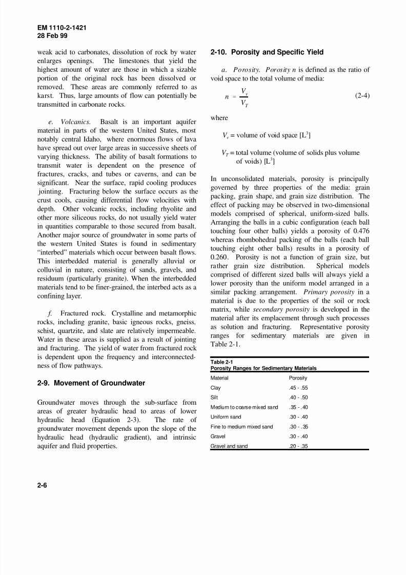
Table 2-1Porosity Ranges for Sedimentary Materials

Material Porosity

Clay .45 - .55

Silt .40 - .50

Medium to coarse mixed sand .35 - .40

Uniform sand .30 - .40

Fine to medium mixed sand .30 - .35

Gravel .30 - .40

Gravel and sand .20 - .35



0

5

10

15

20

25

30

35

40

45

50

C l a y a n d s i l t

F

i n e s a n d

M e d i u m s

a n d

C o a

r s e s a n d

F i n e g r a v e l

M e d i u

m g

r a v e l

C o a r s e g r a v e l

Soil Classification

P e r c e n t

Total Porosity

Specific Yield

Specific Retention

Q ' & KAdh

dl

EM 1110-2-142128 Feb 99

2-7

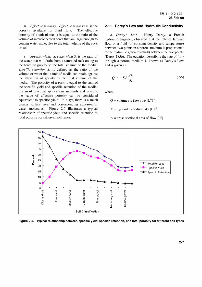
Figure 2-5. Typical relationship between specific yield, specific retention, and total porosity for different soil types

b. Effective porosity. Effective porosity n is thee

porosity available for fluid flow. The effective

porosity of a unit of media is equal to the ratio of the

volume of interconnected pores that are large enough to

contain water molecules to the total volume of the rock

or soil.

c. Specific yield. Specific yield S is the ratio of y

the water that will drain from a saturated rock owing to

the force of gravity to the total volume of the media.

Specific retention Sr is defined as the ratio of the

volume of water that a unit of media can retain against

the attraction of gravity to the total volume of the

media. The porosity of a rock is equal to the sum of

the specific yield and specific retention of the media.

For most practical applications in sands and gravels,

the value of effective porosity can be considered

equivalent to specific yield. In clays, there is a muchgreater surface area and corresponding adhesion of

water molecules. Figure 2-5 illustrates a typical

relationship of specific yield and specific retention to

total porosity for different soil types.

2-11. Darcy’s Law and Hydraulic Conductivity

a. Darcy's Law. Henry Darcy, a French

hydraulic engineer, observed that the rate of laminar

flow of a fluid (of constant density and temperature)

between two points in a porous medium is proportional

to the hydraulic gradient (dh/dl) between the two points

(Darcy 1856). The equation describing the rate of flow

through a porous medium is known as Darcy’s Law

and is given as:

(2-5)

where

Q = volumetric flow rate [L T ]3 -1

K = hydraulic conductivity [LT ]-1

A = cross-sectional area of flow [L ]2



K '

k Dg

µ

v 'Q

A' & K

dh

dl

V x

'Q

ne A

' &Kdh

nedl

EM 1110-2-142128 Feb 99

2-8

h = hydraulic head [L]

l = distance between two points [L]

The negative sign on the right-hand side of Equa-

tion 2-5 (Darcy's Law) is used by convention to

indicate a downward trending flow gradient.

b. Hydraulic conductivity. The hydraulic

conductivity of a given medium is a function of the

properties of the medium and the properties of the

fluid. Using empirically derived proportionality

relationships and dimensional analysis, the hydraulic

conductivity of a given medium transmitting a given

fluid is given as:

(2-6)

where

k = intrinsic permeability of porous medium [L ]2

D = fluid density [ML ]-3

µ = dynamic viscosity of fluid [ML T ]-1 -1

g = acceleration of gravity [LT ]-2

The intrinsic permeability of a medium is a function of

the shape and diameter of the pore spaces. Several

empirical relationships describing intrinsic perme-

ability have been presented. Fair and Hatch (1933)

used a packing factor, shape factor, and the geometric

mean of the grain size to estimate intrinsic perme-

ability. Krumbein (1943) uses the square of the

average grain diameter to approximate the intrinsic

permeability of a porous medium. Values of fluid

density and dynamic viscosity are dependent upon

water temperature. Fluid density is additionally

dependent upon total dissolved solids (TDS). Ranges

of intrinsic permeability and hydraulic conductivity

values for unconsolidated sediments are presented in

Table 2-2.

c. Specific discharge. The volumetric flow

velocity v can be determined by dividing the volumetric

flow rate by the cross-sectional area of flow as:

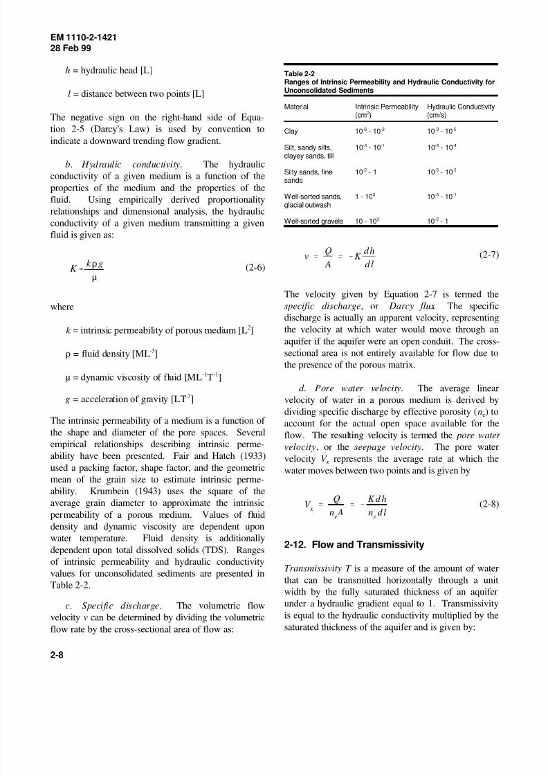
Table 2-2Ranges of Intrinsic Permeability and Hydraulic Conductivity forUnconsolidated Sediments

Material Intrinsic Permeability Hydraulic Conductivity(cm ) (cm/s)2

Clay 10 - 10 10 - 10-6 -3 -9 -6

Silt, sandy silts, 10 - 10 10 - 10clayey sands, till

-3 -1 -6 -4

Silty sands, fine 10 - 1 10 - 10sands

-2 -5 -3

Well-sorted sands, 1 - 10 10 - 10glacial outwash

2 -3 -1

Well-sorted gravels 10 - 10 10 - 13 -2

(2-7)

The velocity given by Equation 2-7 is termed the

specific discharge, or Darcy flux. The specific

discharge is actually an apparent velocity, representing

the velocity at which water would move through an

aquifer if the aquifer were an open conduit. The cross-

sectional area is not entirely available for flow due to

the presence of the porous matrix.

d. Pore water velocity. The average linear

velocity of water in a porous medium is derived by

dividing specific discharge by effective porosity (n ) toe

account for the actual open space available for the

flow. The resulting velocity is termed the pore water

velocity, or the seepage velocity. The pore water

velocity V represents the average rate at which the x

water moves between two points and is given by

(2-8)

2-12. Flow and Transmissivity

Transmissivity T is a measure of the amount of water

that can be transmitted horizontally through a unit

width by the fully saturated thickness of an aquifer

under a hydraulic gradient equal to 1. Transmissivity

is equal to the hydraulic conductivity multiplied by the

saturated thickness of the aquifer and is given by:



K z1

K z2

K x1K x

2

K z1

K z2

K x1K x

2

K z1

K z2

K x1K x

2

K z1

K z2

K x1K x

2

Homogeneous

Isotropic

Kz1 = Kz2

Kx1 = Kx2

Kx = Kz

Homogeneous

Anisotropic

Kz1 = Kz2

Kx1 = Kx2

Kx … Kz

Heterogeneous

Isotropic

Kz1 … Kz2

Kx1 … Kx2

Kx = Kz

Heterogeneous

Anisotropic

Kz1 … Kz2

Kx1 … Kx2

Kx … Kz

T ' Kb

Q x

' K x A

x

)hT

x

EM 1110-2-142128 Feb 99

2-9

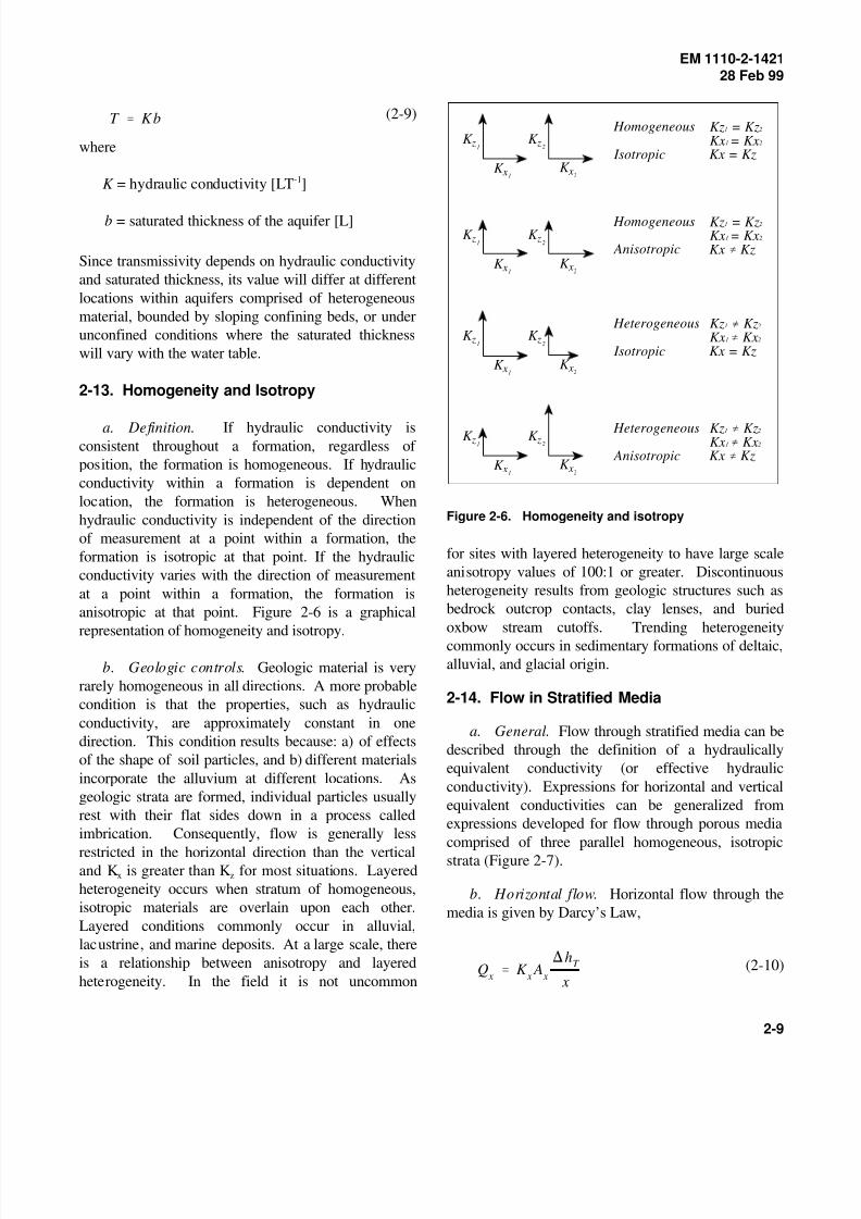
Figure 2-6. Homogeneity and isotropy

(2-9)

where

K = hydraulic conductivity [LT ]-1

b = saturated thickness of the aquifer [L]

Since transmissivity depends on hydraulic conductivity

and saturated thickness, its value will differ at different

locations within aquifers comprised of heterogeneous

material, bounded by sloping confining beds, or under

unconfined conditions where the saturated thickness

will vary with the water table.

2-13. Homogeneity and Isotropy

a. Definition. If hydraulic conductivity isconsistent throughout a formation, regardless of

position, the formation is homogeneous. If hydraulic

conductivity within a formation is dependent on

location, the formation is heterogeneous. When

hydraulic conductivity is independent of the direction

of measurement at a point within a formation, the

formation is isotropic at that point. If the hydraulic

conductivity varies with the direction of measurement

at a point within a formation, the formation is

anisotropic at that point. Figure 2-6 is a graphical

representation of homogeneity and isotropy.

b. Geologic controls. Geologic material is very

rarely homogeneous in all directions. A more probable

condition is that the properties, such as hydraulic

conductivity, are approximately constant in one

direction. This condition results because: a) of effects

of the shape of soil particles, and b) different materials

incorporate the alluvium at different locations. As

geologic strata are formed, individual particles usually

rest with their flat sides down in a process called

imbrication. Consequently, flow is generally less

restricted in the horizontal direction than the verticaland K is greater than K for most situations. Layeredx z

heterogeneity occurs when stratum of homogeneous,

isotropic materials are overlain upon each other.

Layered conditions commonly occur in alluvial,

lacustrine, and marine deposits. At a large scale, there

is a relationship between anisotropy and layered

heterogeneity. In the field it is not uncommon

for sites with layered heterogeneity to have large scale

anisotropy values of 100:1 or greater. Discontinuous

heterogeneity results from geologic structures such as

bedrock outcrop contacts, clay lenses, and buried

oxbow stream cutoffs. Trending heterogeneity

commonly occurs in sedimentary formations of deltaic,alluvial, and glacial origin.

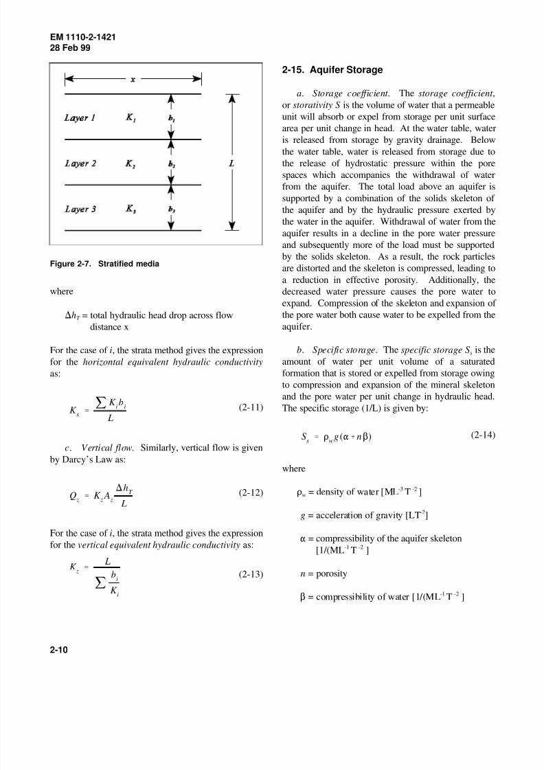
2-14. Flow in Stratified Media

a. General. Flow through stratified media can be

described through the definition of a hydraulically

equivalent conductivity (or effective hydraulic

conductivity). Expressions for horizontal and vertical

equivalent conductivities can be generalized from

expressions developed for flow through porous media

comprised of three parallel homogeneous, isotropic

strata (Figure 2-7).

b. Horizontal flow. Horizontal flow through the

media is given by Darcy’s Law,

(2-10)



K x

' j K i bi

L

Q z

' K z A

z

)hT

L

K z

' L

jb

i

K i

Ss

' Dw

g("% n$)

EM 1110-2-142128 Feb 99

2-10

Figure 2-7. Stratified media

where

)h = total hydraulic head drop across flowT

distance x

For the case of i, the strata method gives the expression

for the horizontal equivalent hydraulic conductivity

as:

(2-11)

c. Vertical flow. Similarly, vertical flow is given

by Darcy’s Law as:

(2-12)

For the case of i, the strata method gives the expression

for the vertical equivalent hydraulic conductivity as:

(2-13)

2-15. Aquifer Storage

a. Storage coefficient. The storage coefficient ,

or storativity S is the volume of water that a permeable

unit will absorb or expel from storage per unit surface

area per unit change in head. At the water table, water

is released from storage by gravity drainage. Below

the water table, water is released from storage due to

the release of hydrostatic pressure within the pore

spaces which accompanies the withdrawal of water

from the aquifer. The total load above an aquifer is

supported by a combination of the solids skeleton of

the aquifer and by the hydraulic pressure exerted by

the water in the aquifer. Withdrawal of water from the

aquifer results in a decline in the pore water pressure

and subsequently more of the load must be supported

by the solids skeleton. As a result, the rock particles

are distorted and the skeleton is compressed, leading toa reduction in effective porosity. Additionally, the

decreased water pressure causes the pore water to

expand. Compression of the skeleton and expansion of

the pore water both cause water to be expelled from the

aquifer.

b. Specific storage. The specific storage S is thes

amount of water per unit volume of a saturated

formation that is stored or expelled from storage owing

to compression and expansion of the mineral skeleton

and the pore water per unit change in hydraulic head.

The specific storage (1/L) is given by:

(2-14)

where

D = density of water [ML T ]w-3 -2

g = acceleration of gravity [LT ]-2

" = compressibility of the aquifer skeleton[1/(ML T ]-1 -2

n = porosity

$ = compressibility of water [1/(ML T ]-1 -2



S ' bSs

S ' S y

% hSs

V w

' SA)h

EM 1110-2-142128 Feb 99

2-11

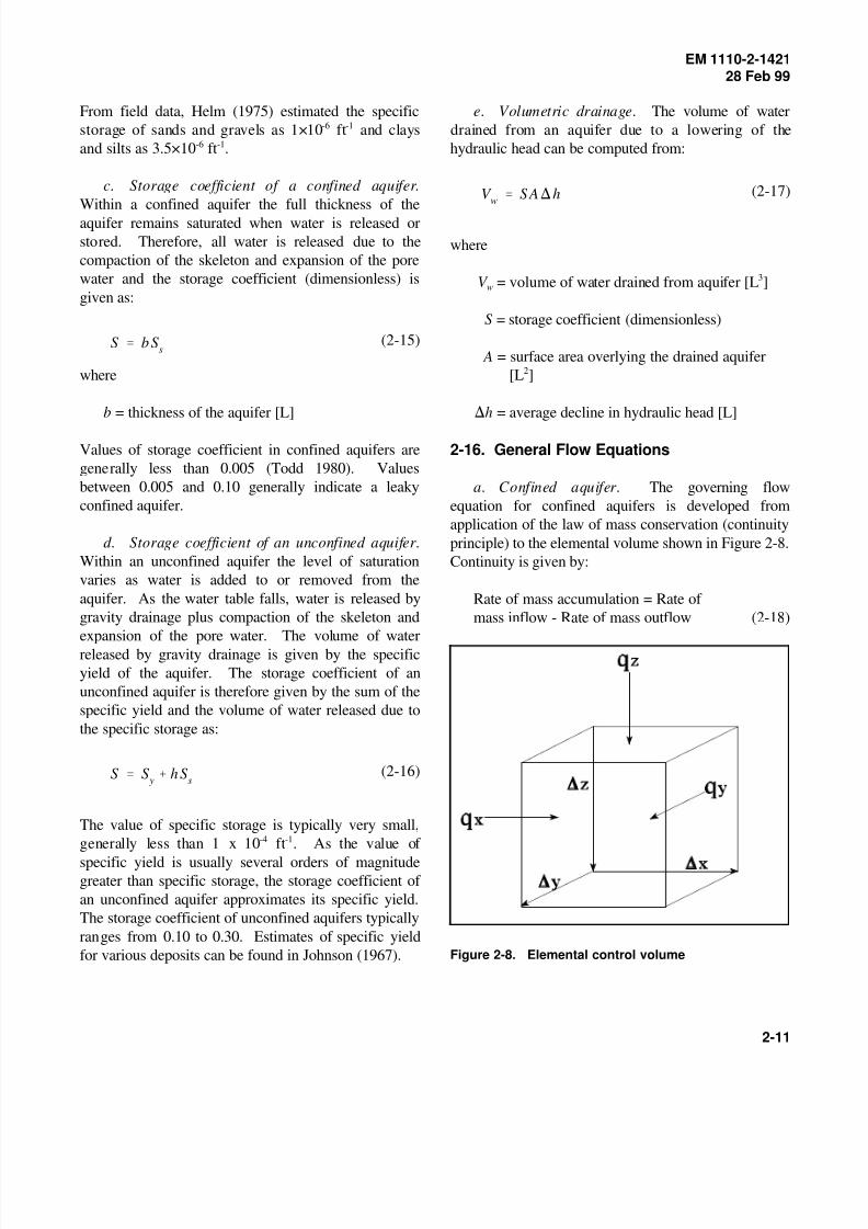
Figure 2-8. Elemental control volume

From field data, Helm (1975) estimated the specific e. Volumetric drainage. The volume of water

storage of sands and gravels as 1×10 ft and clays drained from an aquifer due to a lowering of the-6 -1

and silts as 3.5×10 ft . hydraulic head can be computed from:-6 -1

c. Storage coefficient of a confined aquifer.

Within a confined aquifer the full thickness of the

aquifer remains saturated when water is released or

stored. Therefore, all water is released due to the

compaction of the skeleton and expansion of the pore

water and the storage coefficient (dimensionless) is

given as:

(2-15)

where [L ]

b = thickness of the aquifer [L] )h = average decline in hydraulic head [L]

Values of storage coefficient in confined aquifers are

generally less than 0.005 (Todd 1980). Values

between 0.005 and 0.10 generally indicate a leaky

confined aquifer.

d. Storage coefficient of an unconfined aquifer.

Within an unconfined aquifer the level of saturation

varies as water is added to or removed from the

aquifer. As the water table falls, water is released by

gravity drainage plus compaction of the skeleton and

expansion of the pore water. The volume of water

released by gravity drainage is given by the specific

yield of the aquifer. The storage coefficient of an

unconfined aquifer is therefore given by the sum of the

specific yield and the volume of water released due to

the specific storage as:

(2-16)

The value of specific storage is typically very small,

generally less than 1 x 10 ft . As the value of -4 -1

specific yield is usually several orders of magnitudegreater than specific storage, the storage coefficient of

an unconfined aquifer approximates its specific yield.

The storage coefficient of unconfined aquifers typically

ranges from 0.10 to 0.30. Estimates of specific yield

for various deposits can be found in Johnson (1967).

(2-17)

where

V = volume of water drained from aquifer [L ]w3

S = storage coefficient (dimensionless)

A = surface area overlying the drained aquifer2

2-16. General Flow Equations

a. Confined aquifer. The governing flow

equation for confined aquifers is developed from

application of the law of mass conservation (continuity

principle) to the elemental volume shown in Figure 2-8.

Continuity is given by:

Rate of mass accumulation = Rate of

mass inflow - Rate of mass outflow (2-18)



Ss

Mh

M t '

M

M x K xMh

M x%

M

M y K yMh

M y

%M

M zK

z

Mh

M z

Ss

Mh

M t % W '

M

M xK

x

Mh

M x%

M

M yK

y

Mh

M y

%M

M zK

z

Mh

M z

Ss

Mh

M t ' K

x

M

M x

Mh

M x% K

y

M

M y

Mh

M y

% K z

M

M z

Mh

M z

Ss

Mh

M t ' K

M

M x

Mh

M x%

M

M y

Mh

M y%

M

M z

Mh

M z

Ss

Mh

M t ' K

M2 h

M x 2%

M2 h

M y 2%

M2 h

M z 2

M2 h

M x2

%M

2 h

M y2

%M

2 h

M z2

'S

T

Mh

Mt

M2 h

M x 2%

M2 h

M y 2%

M2 h

M z 2' 0

M

M xK

xhMh

M x%

M

M yK

yhMh

M y%

M

M zK

zhMh

M z

' S y

Mh

M t

M

M xhMh

M x%

M

M yhMh

M y%

M

M zhMh

M z

'

S y

K

Mh

M t

EM 1110-2-142128 Feb 99

2-12

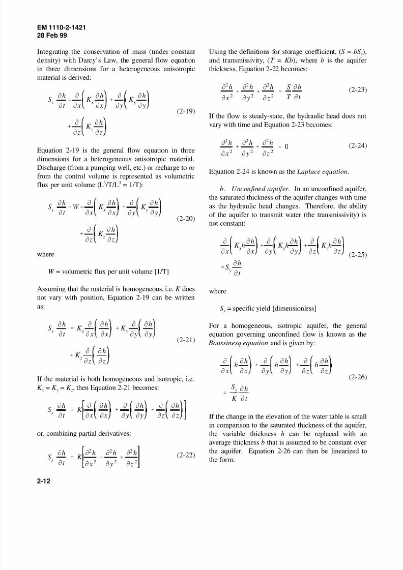
Integrating the conservation of mass (under constant Using the definitions for storage coefficient, (S = bS ),

density) with Darcy’s Law, the general flow equation and transmissivity, (T = Kb), where b is the aquifer

in three dimensions for a heterogeneous anisotropic thickness, Equation 2-22 becomes:

material is derived:

(2-19)

Equation 2-19 is the general flow equation in three

dimensions for a heterogeneous anisotropic material.

Discharge (from a pumping well, etc.) or recharge to or

from the control volume is represented as volumetric

flux per unit volume (L /T/L = 1/T):3 3

(2-20)

where

W = volumetric flux per unit volume [1/T]

Assuming that the material is homogeneous, i.e. K does

not vary with position, Equation 2-19 can be writtenas:

(2-21)

If the material is both homogeneous and isotropic, i.e.

K = K = K , then Equation 2-21 becomes: x y z

or, combining partial derivatives:

(2-22)

s

(2-23)

If the flow is steady-state, the hydraulic head does not

vary with time and Equation 2-23 becomes:

(2-24)

Equation 2-24 is known as the Laplace equation.

b. Unconfined aquifer. In an unconfined aquifer,

the saturated thickness of the aquifer changes with timeas the hydraulic head changes. Therefore, the ability

of the aquifer to transmit water (the transmissivity) is

not constant:

(2-25)

where

S = specific yield [dimensionless] y

For a homogeneous, isotropic aquifer, the general

equation governing unconfined flow is known as the

Boussinesq equation and is given by:

(2-26)

If the change in the elevation of the water table is small

in comparison to the saturated thickness of the aquifer,

the variable thickness h can be replaced with an

average thickness b that is assumed to be constant over

the aquifer. Equation 2-26 can then be linearized to

the form:



M2 h

M x 2%

M2 h

M y 2%

M2 h

M z 2'

S y

Kb

Mh

M t

T

S(M

2 h

M x 2%

M2 h

M y 2%

M2 h

M z 2) '

Mh

M t

q1

' K ) z)h

) x

q1

' K )h ' K )h

T

N d

qT

' q1

% q2

qT

' N f q

1

EM 1110-2-142128 Feb 99

2-13

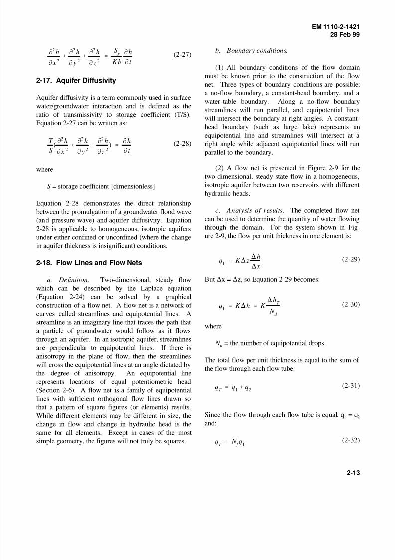
(2-27)

2-17. Aquifer Diffusivity

Aquifer diffusivity is a term commonly used in surfacewater/groundwater interaction and is defined as the

ratio of transmissivity to storage coefficient (T/S).

Equation 2-27 can be written as:

(2-28)

where

S = storage coefficient [dimensionless]

Equation 2-28 demonstrates the direct relationship

between the promulgation of a groundwater flood wave

(and pressure wave) and aquifer diffusivity. Equation

2-28 is applicable to homogeneous, isotropic aquifers

under either confined or unconfined (where the change

in aquifer thickness is insignificant) conditions.

2-18. Flow Lines and Flow Nets

a. Definition. Two-dimensional, steady flow

which can be described by the Laplace equation

(Equation 2-24) can be solved by a graphical

construction of a flow net. A flow net is a network of

curves called streamlines and equipotential lines. A

streamline is an imaginary line that traces the path that

a particle of groundwater would follow as it flows

through an aquifer. In an isotropic aquifer, streamlines

are perpendicular to equipotential lines. If there is

anisotropy in the plane of flow, then the streamlines

will cross the equipotential lines at an angle dictated by

the degree of anisotropy. An equipotential line

represents locations of equal potentiometric head

(Section 2-6). A flow net is a family of equipotentiallines with sufficient orthogonal flow lines drawn so

that a pattern of square figures (or elements) results.

While different elements may be different in size, the

change in flow and change in hydraulic head is the

same for all elements. Except in cases of the most

simple geometry, the figures will not truly be squares.

b. Boundary conditions.

(1) All boundary conditions of the flow domain

must be known prior to the construction of the flow

net. Three types of boundary conditions are possible:

a no-flow boundary, a constant-head boundary, and a

water-table boundary. Along a no-flow boundary

streamlines will run parallel, and equipotential lines

will intersect the boundary at right angles. A constant-

head boundary (such as large lake) represents an

equipotential line and streamlines will intersect at a

right angle while adjacent equipotential lines will run

parallel to the boundary.

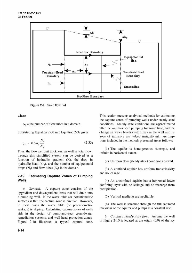
(2) A flow net is presented in Figure 2-9 for the

two-dimensional, steady-state flow in a homogeneous,

isotropic aquifer between two reservoirs with different

hydraulic heads.

c. Analysis of results. The completed flow net

can be used to determine the quantity of water flowing

through the domain. For the system shown in Fig-

ure 2-9, the flow per unit thickness in one element is:

(2-29)

But )x = )z, so Equation 2-29 becomes:

(2-30)

where

N = the number of equipotential dropsd

The total flow per unit thickness is equal to the sum of

the flow through each flow tube:

(2-31)

Since the flow through each flow tube is equal, q = q1 2

and:

(2-32)



qT ' K )hT

N f

N d

EM 1110-2-142128 Feb 99

2-14

Figure 2-9. Basic flow net

where This section presents analytical methods for estimating

N = the number of flow tubes in a domain conditions. Steady-state conditions are approximated f

Substituting Equation 2-30 into Equation 2-32 gives: change in water levels (with time) in the well and its

(2-33)

Thus, the flow per unit thickness, as well as total flow,

through this simplified system can be derived as a

function of hydraulic gradient (K), the drop in

hydraulic head (ªh ), and the number of equipotentialt

drops (N ) and flow tubes (N ) in the domain.d f

2-19. Estimating Capture Zones of Pumping

Wells

a. General. A capture zone consists of the

upgradient and downgradient areas that will drain into

a pumping well. If the water table (or potentiometric

surface) is flat, the capture zone is circular. However,

in most cases the water table (or potentiometric

surface) is sloping. Calculating capture zones of wells

aids in the design of pump-and-treat groundwater

remediation systems, and well-head protection zones.

Figure 2-10 illustrates a typical capture zone.

the capture zones of pumping wells under steady-state

after the well has been pumping for some time, and the

zone of influence are judged insignificant. Assump-

tions included in the methods presented are as follows:

(1) The aquifer is homogeneous, isotropic, and

infinite in horizontal extent.

(2) Uniform flow (steady-state) conditions prevail.

(3) A confined aquifer has uniform transmissivity

and no leakage.

(4) An unconfined aquifer has a horizontal lower

confining layer with no leakage and no recharge from

precipitation.

(5) Vertical gradients are negligible.

(6) The well is screened through the full saturated

thickness of the aquifer and pumps at a constant rate.

b. Confined steady-state flow. Assume the well

in Figure 2-10 is located at the origin (0,0) of the x,y



x '

& y

tan(2BKbiy / Q)

x '

& y

tan[BK (h2

1&h2

2 ) y / QL]

EM 1110-2-142128 Feb 99

2-15

Figure 2-10. Capture zone of a pumping well in plan view. The well is located at the origin (0,0) of the x,y plane

plane. The equation to describe the edge of the capture The maximum width of the capture zone as the

zone (groundwater divide) for a confined aquifer when distance (x) upgradient from the pumping well

steady-state conditions have been reached is (Grubb approaches infinity is given by (Todd 1980):

1993):

(2-34)

where

Q = pumping rate [L /T]3

K = hydraulic conductivity [L/T]

b = aquifer thickness [L]

i = hydraulic gradient of the flow field in the

absence of the pumping well (dh/dx) and

tan (*) is in radians.

The distance from the pumping well downstream to the

stagnation point that marks the end of the capture zone

is given by:

x = -Q/(2BKbi) (2-35)0

y = Q/Kbi (2-36)c

c. Unconfined steady-state flow. Assume the

well in Figure 2-10 is located at the origin (0,0) of thex,y plane. The equation to describe the edge of the

capture zone (groundwater divide) for an unconfined

aquifer when steady-state conditions have been reached

is (Grubb 1993):

(2-37)

where

Q = pumping rate [L /T]3

K = hydraulic conductivity [L/T]

h = upgradient head above lower boundary of 1

aquifer prior to pumping



N

GW Flow Direction

2,000 m

400 mMunicipal Well

Q = 19,250 m3 /day

Toxic Spill

x '& y

tan(2BKbiy / Q)

EM 1110-2-142128 Feb 99

2-16

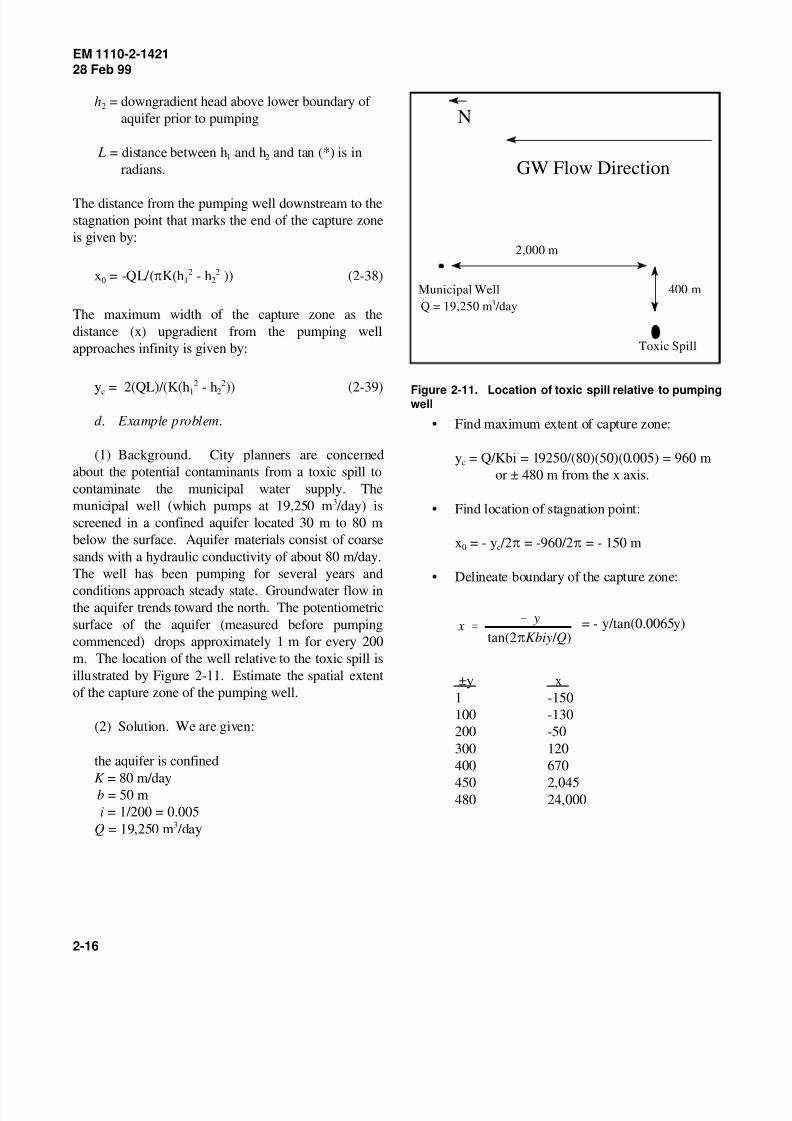
Figure 2-11. Location of toxic spill relative to pumpingwell

h = downgradient head above lower boundary of 2

aquifer prior to pumping

L = distance between h and h and tan (*) is in1 2

radians.

The distance from the pumping well downstream to the

stagnation point that marks the end of the capture zone

is given by:

x = -QL/(BK(h - h )) (2-38)0 1 22 2

The maximum width of the capture zone as the

distance (x) upgradient from the pumping well

approaches infinity is given by:

y = 2(QL)/(K(h - h )) (2-39)c 1 2

2 2

d. Example problem.

(1) Background. City planners are concerned

about the potential contaminants from a toxic spill to

contaminate the municipal water supply. The

municipal well (which pumps at 19,250 m /day) is3

screened in a confined aquifer located 30 m to 80 m

below the surface. Aquifer materials consist of coarse

sands with a hydraulic conductivity of about 80 m/day.

The well has been pumping for several years and

conditions approach steady state. Groundwater flow inthe aquifer trends toward the north. The potentiometric

surface of the aquifer (measured before pumping

commenced) drops approximately 1 m for every 200

m. The location of the well relative to the toxic spill is

illustrated by Figure 2-11. Estimate the spatial extent

of the capture zone of the pumping well.

(2) Solution. We are given:

the aquifer is confined

K = 80 m/day

b = 50 m

i = 1/200 = 0.005

Q = 19,250 m /day3

• Find maximum extent of capture zone:

y = Q/Kbi = 19250/(80)(50)(0.005) = 960 mc

or ± 480 m from the x axis.

• Find location of stagnation point:

x = - y /2B = -960/2B = - 150 m0 c

• Delineate boundary of the capture zone:

= - y/tan(0.0065y)

±y x

1 -150

100 -130

200 -50

300 120

400 670

450 2,045480 24,000



EM 1110-2-142128 Feb 99

2-17

(3) Analysis of results. The capture zone at a turbulent where Darcy’s law rarely applies. Solution

distance x = 2,000 m from the pumping well extends channels leading to high permeability are favored in

450 m from the horizontal (x) axis. Therefore, initial areas where topographic, bedding, or jointing features

calculations indicate that a portion of the contaminant promote flow localization which focuses the solvent

plume will contaminate the municipal water supply action of circulating groundwater, or well-connected

unless mitigative measures are taken. Further pathways exist between recharge and discharge zones,

investigation is warranted. favoring higher groundwater velocities (Smith and

2-20. Specialized Flow Conditions

a. General. Darcy's Law (Section 2-11) is an

empirical relationship which is only valid under the

assumption of constant density and laminar flow.

These assumptions are not always met in nature. Flow

conditions in which Darcy's Law is not necessarily

applicable are cited below.

(1) Fractured flow. Fractured-rock aquifers occurin environments in which the flow of water is primarily

through fractures, joints, faults, or bedding planes

which have not been significantly enlarged by

dissolution. Fracturing adds secondary porosity to a

soil medium that already has some original porosity.

The original porosity consists of pores that are roughly

similar in length and width. These pores interconnect to

form a tortuous water network for groundwater flow.

Fractured porosity is significantly different. The

fractures consist of pathways that are much greater in

length than width. These pathways provide conduits for

groundwater flow that are much less tortuous than the

original porosity. At a local scale, fractured rock can

be extremely heterogeneous. Effective permeability of

crystalline rock typically decreases by two or three

orders of magnitude in the first thousand feet below

ground surface, as the number of fractures decrease or

close under increased lithostatic load (Smith and

Wheatcraft 1992).

(2) Karst aquifers. Karst aquifers occur in

environments where all or most of the flow of water is

through joints, faults, bedding planes, pores, cavities,conduits, and caves, any or all of which have been

significantly enlarged by dissolution. Effective

porosity in karst environments is mostly tertiary, where

secondary porosity is modified by dissolution through

pores, bedding planes, fractures, conduits, and caves.

Karst aquifers are generally highly anisotropic and

heterogeneous. Flow in karst aquifers is often fast and

Wheatcraft 1992).

(3) Permafrost. Temperatures significantly below

0E C are required to produce permafrost. The depth

and location of frozen water within the soil depends

upon many factors such as fluid pressure, salt content

of the pore water, the grain size distribution of the soil,

soil mineralogy, and the soil structure. The presence of

frozen or partially frozen groundwater has a

tremendous effect upon flow. As water freezes, it

expands to fill pore spaces. Soil that normally conveyswater easily becomes an aquitard or aquiclude when

frozen. The flow of water in permafrost regions is

analogous to fractured flow environments where flow

is confined to conduits in which complete freezing has

not taken place.

(4) Variable-density flow. Unlike aquifers con-

taining constant-density water, where flow is controlled

only by the hydraulic head gradient and the hydraulic

conductivity, variable-density flow is also affected by

change in the spatial location within the aquifer. Water

density is commonly affected by temperature, or totaldissolved solids. As water temperature increases, its

density decreases. A temperature gradient across an

area influences the measurements of hydraulic head

and the corresponding hydraulic gradient. Intrinsic

hydraulic conductivity is also a function of water

temperature (Equation 2-6). Thus, it is important to

assess effects of fluid density on hydraulic gradient and

hydraulic gradient in all site investigations.

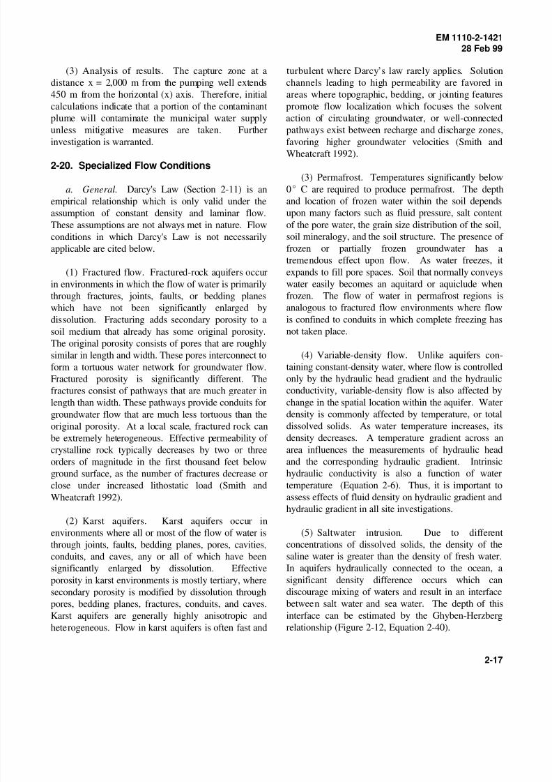
(5) Saltwater intrusion. Due to different

concentrations of dissolved solids, the density of thesaline water is greater than the density of fresh water.

In aquifers hydraulically connected to the ocean, a

significant density difference occurs which can

discourage mixing of waters and result in an interface

between salt water and sea water. The depth of this

interface can be estimated by the Ghyben-Herzberg

relationship (Figure 2-12, Equation 2-40).



zs'

D f

Ds&D

f

zw

zs' 40 z

w

EM 1110-2-142128 Feb 99

2-18

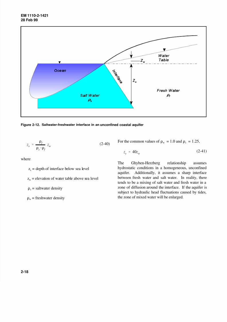
Figure 2-12. Saltwater-freshwater interface in an unconfined coastal aquifer

(2-40)

where

z = depth of interface below sea levels

z = elevation of water table above sea levelw

D = saltwater densitys

D = freshwater densityw

For the common values of D = 1.0 and D = 1.25,w s

(2-41)

The Ghyben-Herzberg relationship assumes

hydrostatic conditions in a homogeneous, unconfinedaquifer. Additionally, it assumes a sharp interface

between fresh water and salt water. In reality, there

tends to be a mixing of salt water and fresh water in a

zone of diffusion around the interface. If the aquifer is

subject to hydraulic head fluctuations caused by tides,

the zone of mixed water will be enlarged.

Documents

Occurrence and Movement of Groundwater