Ocean modeling - UiO

Ocean modelingKai H. Christensen

Division for Ocean and Ice, R&D Department

OGCM● OGCM = ocean general circulation model.● Solves primitive equations for the state of the ocean.● Typically a community model (open source) with large user base.● Typically written in Fortran and optimized for speed.● Examples:

- HYCOM

- NEMO

- POM

- MITgcm

- MOM

- FVCOM

- ROMS

(Hedstrom, 2015)

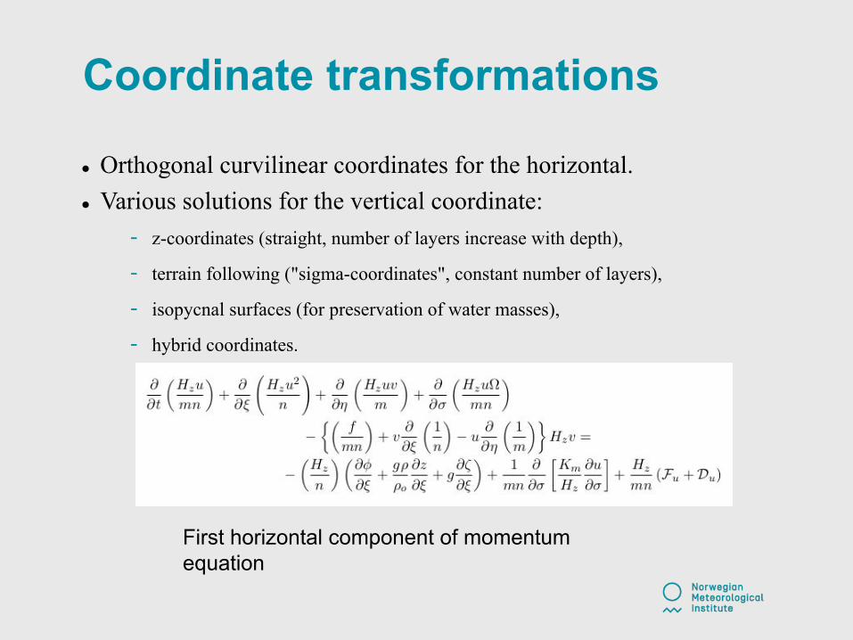
Coordinate transformations

● Orthogonal curvilinear coordinates for the horizontal.● Various solutions for the vertical coordinate:

- z-coordinates (straight, number of layers increase with depth),

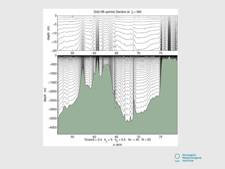
- terrain following ("sigma-coordinates", constant number of layers),

- isopycnal surfaces (for preservation of water masses),

- hybrid coordinates.

First horizontal component of momentum equation

(Røed et al., 2016)

Discretization● The time-space domain is

discretized and the equations recast as finite differences*.

● The aspect ratio is large! Horizontal grid spacing is typically 1-50 km, vertical grid spacing 0.1-100 m.

● Numerical stability depends on how the equations are discretized.

* In most OGCMs.

Staggered grids

● Staggered grids are often used, in which velocity and tracer variables are not co-located.

● ROMS uses the Arakawa C grid.

● CICE uses the Arakawa B grid (with some modifications).

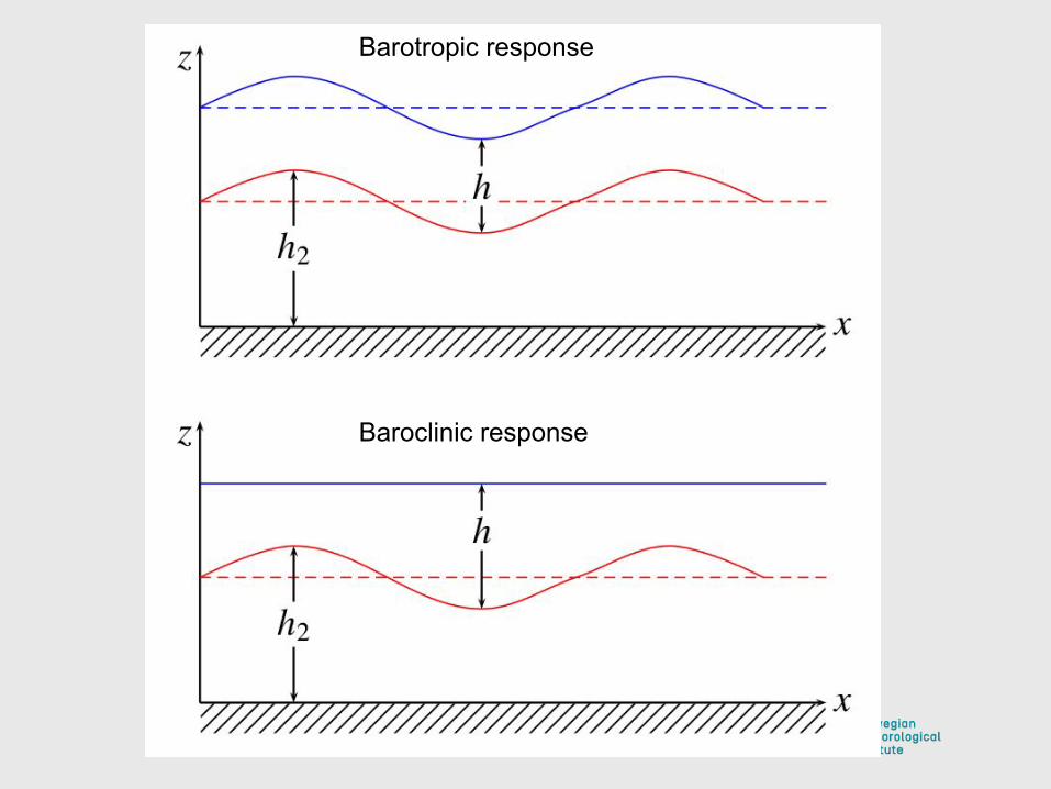
Barotropic response

Baroclinic response

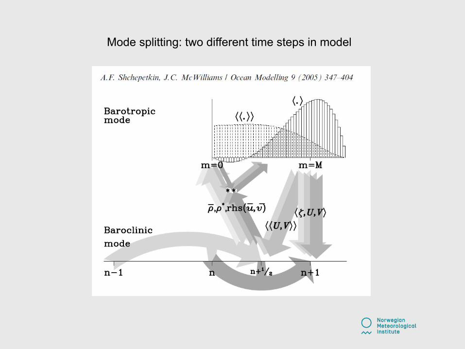
Mode splitting: two different time steps in model

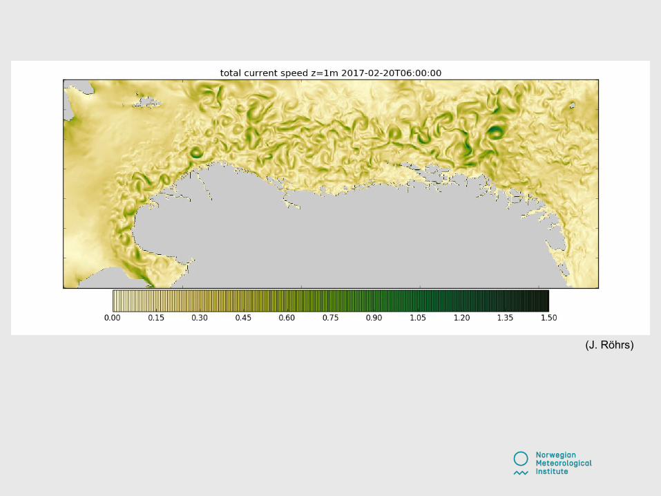
(J. Röhrs)

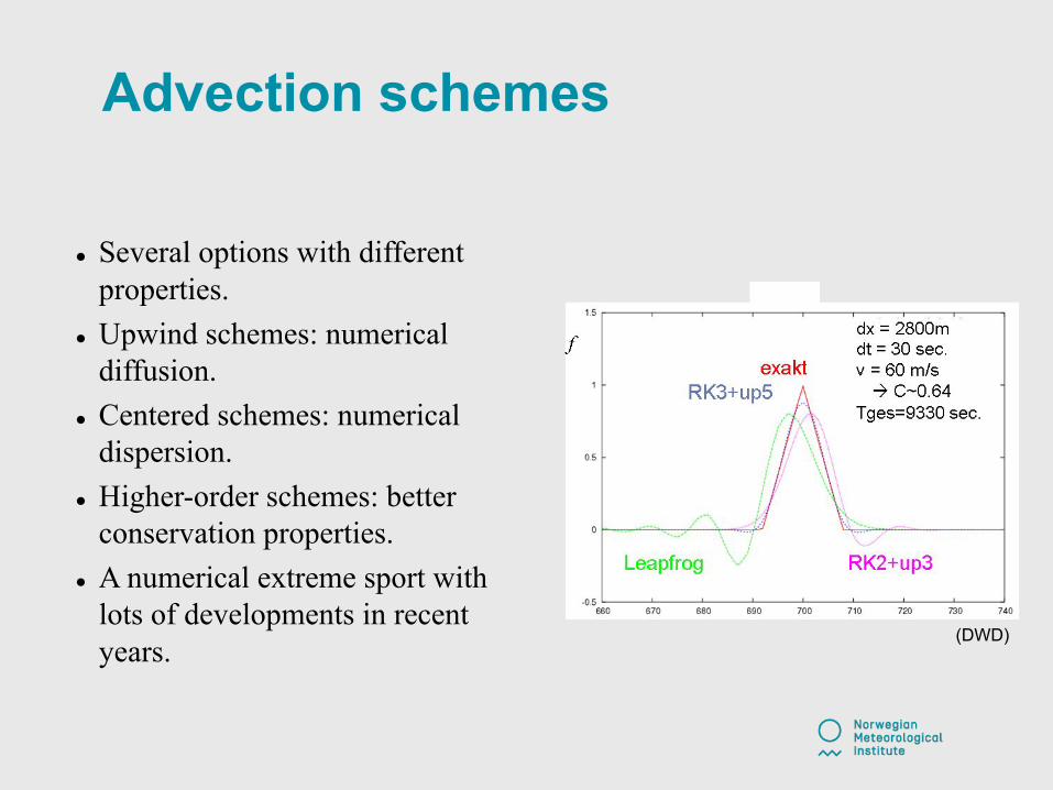
https://docs.google.com/file/d/11j6OyGiDvkj2GG_bF6MZHIqFWgDn-Nx7/preview

Advection schemes

● Several options with different properties.

● Upwind schemes: numerical diffusion.

● Centered schemes: numerical dispersion.

● Higher-order schemes: better conservation properties.

● A numerical extreme sport with lots of developments in recent years.

(DWD)

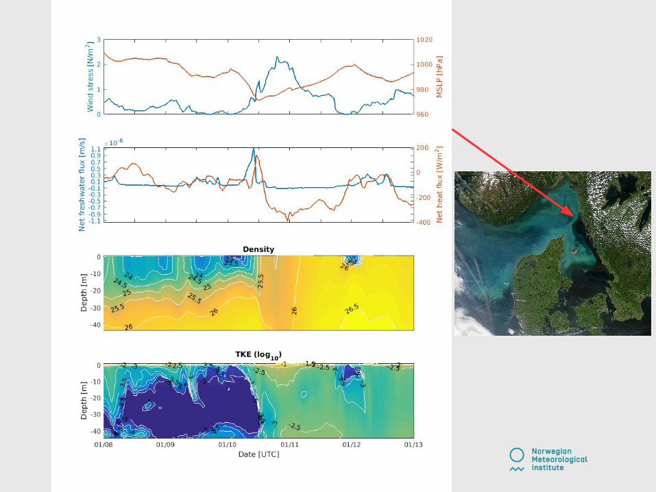
Vertical mixing

● Separate routines for calculating exchange coefficients for vertical turbulent mixing (eddy viscosity, eddy diffusivities).

● Critical part of the modeling system for operational use.● Several options ranging from simple diagnostic schemes to full

prognostic two-equation systems for turbulence kinetic energy (TKE) and turbulence length/time scales (e.g. k-ε).

● Two-equation systems are CPU-intensive (~30% of the resources).● Surface waves are important.

Norwegian Meteorological Institue<footer>19

(Janssen, 2012)

TKE – turb.fluctuations

2D wave spectrum

mean hor. velocity shear

salinity and temperature profiles

turbulence dissipation ratepressure and vert. velocity

fluctuationsTKE, turb. length scaleand stratification


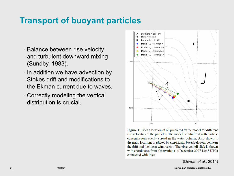
Transport of buoyant particles

· Balance between rise velocity and turbulent downward mixing (Sundby, 1983).

· In addition we have advection by Stokes drift and modifications to the Ekman current due to waves.

· Correctly modeling the vertical distribution is crucial.

(Drivdal et al., 2014)


Forcing

· The ocean model requires fluxes on all physical boundaries for

- momentum,- energy (heat, TKE), and- mass (precipitation and rivers).

· Ideally, the ocean model should be fully coupled to the models for the atmosphere, the sea ice, and the waves.

· The ocean has a long memory, and errors in the forcing are detrimental for the final result (rubbish in = rubbish out).


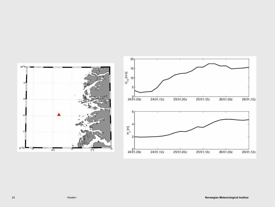
Atmospheric forcing

· Either use bulk flux algorithms: provide e.g. 10 m winds, 2 m temperature, relative humidity etc., and calculate fluxes using parameterizations,

· or provide the fluxes directly from a stand-alone or coupled modeling system.

· Sea ice and surface waves greatly influence the air-sea fluxes.




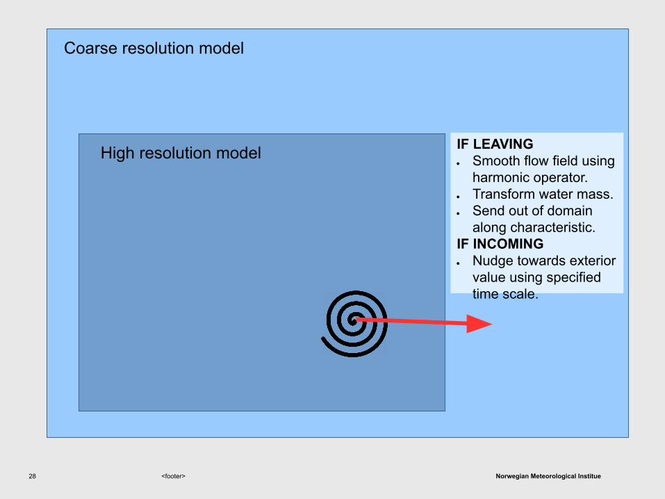
Lateral boundary conditions in regional ocean modeling

· The downscaling from a coarse resolution to a high resolution model is called "nesting".

· We differ between full two-way nesting, which is fine, and one-way nesting, which constitutes an ill-posed mathematical problem (and is unfortunately most common).

Coarse resolution model

High resolution model







IF LEAVING● Smooth flow field using

harmonic operator.● Transform water mass.● Send out of domain

along characteristic. IF INCOMING● Nudge towards exterior

value using specified time scale.


<footer>30

ATMOSPHERIC MODEL

WAVE MODEL ICE MODEL

BOUNDARIES

MIXING

KERNEL

NL TL AD

OCEAN MODEL

Ocean+ modeling:

Improved physics by coupling model components.

<footer>31

<footer>32

<footer>33

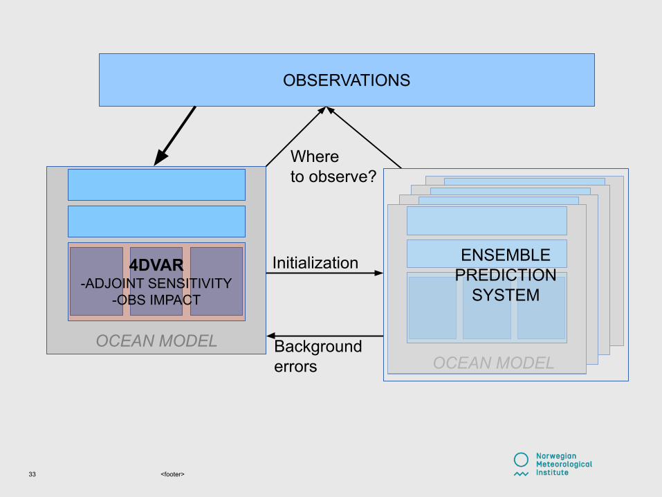
4DVAR-ADJOINT SENSITIVITY

-OBS IMPACT

OCEAN MODEL

OBSERVATIONS

Initialization

Backgrounderrors

Whereto observe?

OCEAN MODEL

ENSEMBLEPREDICTION

SYSTEM

OCEAN MODELOCEAN MODEL

ENSEMBLEPREDICTION

SYSTEM


ENSEMBLEPREDICTION

SYSTEM


ENSEMBLEPREDICTION

SYSTEM

OCEAN MODEL

ENSEMBLEPREDICTION

SYSTEM

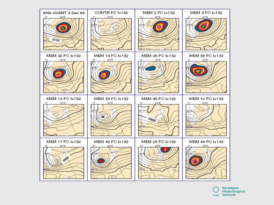
Ensemble prediction systems

● An EPS consists of several instances of a model with slightly perturbed physical forcing and/or initial conditions

● The difference between the ensemble members reflect the uncertainties in the model, and can be used to assess multivariate error covariances (ensemble Kalman filters)

● The challenge is to have a realistic spread in the ensemble, and to avoid ensemble collapse

● EPS verification is based on a basic hypothesis: the ensemble members and the observations are drawn from the same probability distribution

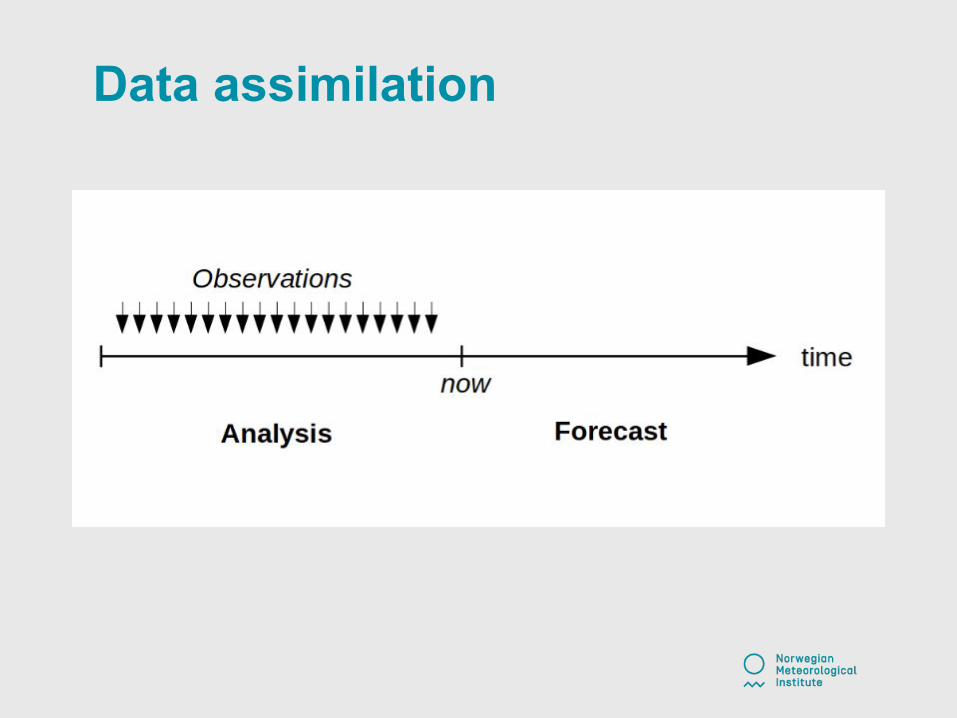
Data assimilation

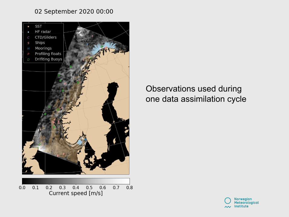
Observations used duringone data assimilation cycle

Summary

● Ocean general circulation models are complex tools for estimating the physical state of the ocean.

● There is no "best" model, only one "best" model for a particular purpose, and that model can be improved.

● Due to limitations in computing resources, we will struggle with unresolved dynamical processes in the foreseeable future.

● Data assimilation provides the best estimate of the physical state of the ocean in the entire space-time domain of the model.

● Progress is expected due to model coupling efforts and increased availability of observations in near-real-time.

Documents

Ocean modeling - UiO