This article was downloaded by: [Tufts University]On: 05 May 2014, At: 11:01Publisher: Taylor & FrancisInforma Ltd Registered in England and Wales Registered Number: 1072954 Registeredoffice: Mortimer House, 37-41 Mortimer Street, London W1T 3JH, UK

International Journal of RemoteSensingPublication details, including instructions for authors andsubscription information:http://www.tandfonline.com/loi/tres20

Ocean surface Stokes drift fromscatterometer observationsGuoqiang Liua, William A. Perriea & Yijun Heb

a Bedford Institute of Oceanography, Fisheries and OceansCanada, Dartmouth, NS, Canada B2Y 4A2b School of Marine Sciences, Nanjing University of InformationScience and Technology, Nanjing 210044, ChinaPublished online: 26 Feb 2014.

To cite this article: Guoqiang Liu, William A. Perrie & Yijun He (2014) Ocean surface Stokes driftfrom scatterometer observations, International Journal of Remote Sensing, 35:5, 1966-1978, DOI:10.1080/01431161.2014.880818

To link to this article: http://dx.doi.org/10.1080/01431161.2014.880818

PLEASE SCROLL DOWN FOR ARTICLE

Taylor & Francis makes every effort to ensure the accuracy of all the information (the“Content”) contained in the publications on our platform. However, Taylor & Francis,our agents, and our licensors make no representations or warranties whatsoever as tothe accuracy, completeness, or suitability for any purpose of the Content. Any opinionsand views expressed in this publication are the opinions and views of the authors,and are not the views of or endorsed by Taylor & Francis. The accuracy of the Contentshould not be relied upon and should be independently verified with primary sourcesof information. Taylor and Francis shall not be liable for any losses, actions, claims,proceedings, demands, costs, expenses, damages, and other liabilities whatsoever orhowsoever caused arising directly or indirectly in connection with, in relation to or arisingout of the use of the Content.

This article may be used for research, teaching, and private study purposes. Anysubstantial or systematic reproduction, redistribution, reselling, loan, sub-licensing,systematic supply, or distribution in any form to anyone is expressly forbidden. Terms &Conditions of access and use can be found at http://www.tandfonline.com/page/terms-and-conditions

Ocean surface Stokes drift from scatterometer observations

Guoqiang Liua, William A. Perriea*, and Yijun Heb

aBedford Institute of Oceanography, Fisheries and Oceans Canada, Dartmouth, NS, CanadaB2Y 4A2; bSchool of Marine Sciences, Nanjing University of Information Science and Technology,

Nanjing 210044, China

(Received 1 October 2012; accepted 26 October 2013)

Stokes drift, a mean Lagrangian motion induced by ocean surface gravity waves, playsan important role in modifying the upper ocean circulation. In this study, two empiricalmodels are developed to estimate ocean surface Stokes drift Uss, based on a multilayer-perceptron Back-Propagation Neural Network (BP NN) algorithm, using buoy datacollocated with European Remote Sensing (ERS) data, and using (1) bulk waveparameters and (2) spectral wave density. Both BP NN models perform reasonablywell, with correlation coefficients of 0.92 between the retrieved Uss and buoy mea-surements, for the former bulk-parameter-based NN model, compared to 0.87, for thelatter spectral wave-density-based NN model. Uss values were estimated over theglobal ocean during 27–29 August 1998. We found Uss in the range from 2 to36 cm s−1 with an average of 9 cm s−1, which is in good agreement with previousobservations. With the retrieved Uss, we calculated the Langmuir number Lat and thescaled Langmuir vertical turbulent velocity. The distribution of Lat (generally in therange 0.25–0.58) provides a measure of the dominance of Langmuir turbulence overkinetic energy turbulence in regions with high Uss, such as the westerlies in theSouthern Ocean.

1. Introduction

Stokes drift, defined as the difference between the average Lagrangian velocity of afluid parcel and the Eulerian current at a fixed point (Stokes 1847), plays an importantrole in mass fluxes and ocean surface circulation (e.g. McWilliams et al. 1999). Recentstudies suggest that ocean surface Stokes drift Uss accounts for two-thirds of thesurface wind-induced drift in the open oceans. Thus, at times, Uss determines thefate of oil pollutions and larvae recruitment (Ardhuin et al. 2004, 2008; Kantha andClayson 2004; Rascle, Ardhuin, and Terry 2006; Rascle et al. 2008). Furthermore,Stokes drift is crucial for dynamic processes in the oceanic mixed layer. On the onehand, Stokes drift dissipation enhances the upper ocean layer turbulence and its effectscan be felt potentially throughout the entire mixed layer (Kantha et al. 2009). On theother hand, the non-linear interaction between wind-driven mean currents and Stokesdrift generates Langmuir circulation, which is believed to deepen the mixed layer andsignificantly complicate the upper ocean dynamics (e.g. Craik and Leibovich 1976;Leibovich 1980, 1983; Li, Zahariev, and Garrett 1995; Noh, Gahyun, and Siegfried2011).

Given the vital importance of Stokes drift in the upper ocean dynamics, it isnecessary and urgent to estimate the magnitude and distribution of Uss over the global

*Corresponding author. Email: William.Perrie@dfo-mpo.gc.ca

International Journal of Remote Sensing, 2014Vol. 35, No. 5, 1966–1978, http://dx.doi.org/10.1080/01431161.2014.880818

© 2014 Her Majesty the Queen in right of Canada

Dow

nloa

ded

by [

Tuf

ts U

nive

rsity

] at

11:

01 0

5 M

ay 2

014

oceans. However, there is a paucity of in situ observations of Stokes drift over openoceans, although coastal North American buoy data are available. Recently, Rascle et al.(2008) used numerical wave model results to estimate Uss over the global ocean. Kanthaet al. (2009) also estimated the Stokes drift dissipation from wave model results. Bymeans of ocean wave models, we can indeed obtain the distribution of Uss over theglobal oceans, obtaining estimates that are in good agreement with buoy-derived results.However, the results tend to be limited by the reliability of atmospheric wind input data,and unsolved wave model physics (e.g. non-linear wave–wave interactions, and wavedissipation). Alternately, empirical formulae for estimating Uss have been developed.For example, McWilliams et al. (1999) parameterized Uss as simply a function of thewind vector and ocean depth, assuming that the ocean waves are fully developed,although that is clearly not the case in situations where winds are rapidly changing,such as developing cyclones (Hanley, Belcher, and Sullivan 2010). As another example,Ardhuin et al. (2009) proposed an accurate empirical formula that is a function of windspeed U10 and significant wave height H. However, the altimeter’s nadir-pointinggeometry only permits estimates of wave height and wind speed along a very narrowswath (~2 km). Therefore, we cannot obtain reliable synoptic-scale estimates for Uss

over the global ocean from altimeter-retrieved data, because the Stokes drift changesrapidly owing to variability in the forcing winds and sea state, which are alwayschanging.

The scatterometer sensor can obtain ocean surface winds from model functions ofBragg scattering owing to ocean surface roughness. It is well known that sea state canmodulate the Bragg waves, thus affecting the backscatter signals. Quilfen, Chapron, andVandemark (2001) reported that the highest correlations are obtained between (H/T) andthe measured minus predicted backscatter cross-sections (σ0), as well as between (H/T2)and again the measured minus predicted σ0; here, T is the average wave period. Using alarge collocated data set of scatterometer and buoy measurements, Quilfen et al. (2004)found that the σ0 dependency is not strictly related to the significant slope parameter(~H/T2); rather, it depends on a combination of the significant slope parameter and thesquare root of the significant orbital velocity (~H/T). Uss can be scaled following wavebulk parameters ~ (H2/T3), written as (~H/T2· H/T). Therefore it is reasonable to suggestthat the non-linear relationship may potentially be represented in terms of the backscatterσ0 and Uss.

Another reason to suggest that the scatterometer has the ability to retrieve Uss is thatthe wind speed from the geophysical model function corresponds to the upper frequencypart of the ocean wave spectrum, which is the dominant contribution to Uss. Moreover,σ0 also reflects sea state (wave slope and wave age), which modifies and contributes toUss (Liu et al. 2011; Guo et al. 2009). In addition, scatterometer observations provideglobally distributed backscatter data on synoptic timescales. This implies that there is anopportunity to explore the capability of the scatterometer to retrieve global-scale valuesfor Uss.

In this study, we construct BP NN algorithms to retrieve Uss from the ERS-1/2scatterometer products, following Liu et al. (2011). Section 2 introduces the data,describes the BP NN methodology used for the retrievals, and presents two empiricalformulae to estimate Uss. Section 3 discusses the spatial distribution of Uss retrieved fromthe ERS-2 scatterometer for the period 27–29 August 2008 over the global ocean, basedon a newly developed BP NN model. Section 4 presents a discussion of the characteristicsof Langmuir circulation by considering the Langmuir number and the scaled Langmuirturbulent vertical velocity. Conclusions are provided in Section 5.

International Journal of Remote Sensing 1967

Dow

nloa

ded

by [

Tuf

ts U

nive

rsity

] at

11:

01 0

5 M

ay 2

014

2. Methods

2.1. Data selection

Microwave scatterometer data became available with the launch of the ERS-1 spacecraftin July 1991, which operated simultaneously with the ERS-2 satellite from April 1995 toMarch 2000, transmitting and receiving vertically polarized signals at 5.3 GHz, with anoverall swath width of 475 km, resulting from 19 cells, each covering 25 km. Thus, theBP NN training and validation data are derived from collocations of ERS-1/2 observationsand in situ data taken from 12 National Data Buoy Center (NDBC) buoys. Buoys far fromthe coast (>50 km) are chosen to avoid the effects of the coastline. The maximum spatialdifferences between buoy wave data and satellite scatterometer data are required to be lessthan 0.15° in latitude and longitude, and the maximum time difference is required to beless than 0.5 hours.

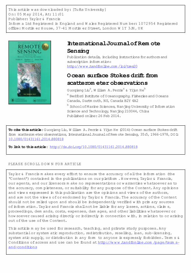
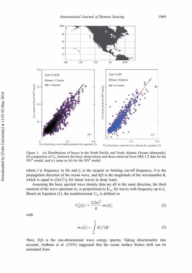
A total of 10,485 pairs of ERS-1/2 scatterometer observations and corresponding buoywave bulk parameter data were obtained. Because spectral wave density data were notprovided by NDBC buoys until 1996, we only obtained 5092 data pairs of ERS-1/2scatterometer observations and corresponding spectral wave density data from buoys.Moreover, 4866 collocated data are obtained among satellite, buoy wave bulk parameter,and buoy spectral wave density data. The buoy locations are shown in Figure 1(a), in deepwater, with an average depth of 2212 m and a minimum depth of 88 m.

2.2. Back-propagation NN model for inversion of ERS-1/2 data

A BP NN methodology defines a computational architecture for complex data processingusing sets of several simple processors called neurons. Inside the NN, all neurons aredecomposed into non-overlying subsets (layers) that are interconnected by neuron weightsand bias coefficients via transfer functions. NNs are widely used in satellite remote-sensing studies (Goodberlet and Swift 1992; Smith 1993; Krasnopolsky 2007). Thenetwork has at least three layers: input layer, hidden layer, and output layer. The inputlayer distributes the input parameters to the hidden layer, consisting of a varying numberof neurons, where each input parameter is multiplied by its connection’s weight parameterand all the inputs to the neurons are summed and passed through the transfer function.The third (output) layer receives the output of the hidden layer, where it is again processedby the neurons (Keiner et al. 1998). In this study, the input data include the incidenceangles (θ), and values of cos(Φ – φ), where Φ is the azimuth angle and φ is the winddirection, normalized radar backscatter cross-sections (σ0), whereas U10 data are takenfrom the ERS-1/2 level1B products.

Because one wind vector corresponds to three independent backscatter measurements,obtained by three different viewing directions, we have three sets of input data for eachcollocated buoy data set. Here, all three sets of data are used to train and validate themodel. The output data are the ocean surface Stokes drift calculated from two methods.One method is based on the ocean wave directional spectral data E(f,θ); in this case, theocean surface Stokes drift vector Uss for waves with frequencies up to fc can be written as(Kenyon 1969)

U ss ¼ 4πZfc0

Z2π0

f k f ; #ð ÞE f ; θð Þdfd#; (1)

1968 G. Liu et al.

Dow

nloa

ded

by [

Tuf

ts U

nive

rsity

] at

11:

01 0

5 M

ay 2

014

where f is frequency in Hz and fc is the nyquist or limiting cut-off frequency, θ is thepropagation direction of the ocean wave, and k(f) is the magnitude of the wavenumber k,which is equal to (2πf )2/g for linear waves in deep water.

Assuming the buoy spectral wave density data are all in the same direction, the thirdmoment of the wave spectrum m3 is proportional to Uss, for waves with frequency up to fc.Based on Equation (1), the nondirectional Uss is defined as

U 1ss fcð Þ ¼ 2 2πð Þ2

gm3 fcð Þ (2)

with

m3 fcð Þ ¼Zfc0

E fð Þdf : (3)

Here, E(f) is the one-dimensional wave energy spectra. Taking directionality intoaccount, Ardhuin et al. (2009) suggested that the ocean surface Stokes drift can beestimated from

60N

48

36

24

12

180

0.4

Corr = 0.918

Rmse = 1.7cm/s

Nb = 1.9cm/s

Corr = 0.87

Rmse = 3.6cm/s

Nb = 3.1cm/s0.3

0.2

Uss

ret

riev

ed f

rom

NN

A m

odel

Uss

ret

riev

ed f

rom

NN

S mod

el

0.1

0 0.2Uss from buoy wave bulk parameter by eqaution (5) Uss from buoy spectral wave density by eqaution (3)

0.4 0.2 0.4

150 120 90 60W

(a)

(b) (c)

Figure 1. (a) Distributions of buoys in the North Pacific and North Atlantic Oceans (diamonds),(b) comparison of Uss between the buoy observations and those retrieved from ERS-1/2 data for theNNA model, and (c) same as (b) for the NNS model.

International Journal of Remote Sensing 1969

Dow

nloa

ded

by [

Tuf

ts U

nive

rsity

] at

11:

01 0

5 M

ay 2

014

USss fcð Þ ffi 0:85U1

ss fcð Þ; (4)

for typical wave spectra, based on Equations (1) and (2). The second method follows thesemi-empirical equation also proposed by Ardhuin et al. (2009):

UAss fcð Þ ffi 5:0� 10�4 5

4� 1

4

fc2

� �13

" #U10 � min U10; 14:5f g þ 0:025 H � 0:4ð Þ; (5)

where H and U10 are both measured by the buoys. Here, fc is taken as 0.4 Hz, which isestimated to be the upper limit for reliable buoy measurements.

For comparison, we also calculated Uss using bulk wave parameters, specifically thesignificant wave height and the peak period Tp, from Tamura, Miyazawa, and Oey (2012),written as

Ubss ¼ π3H2=gT 3

p : (6)

Based on the collocated scatterometer data, buoy bulk wave parameters, and buoy spectraldensity data, Table 1 provides a comparison of Uss estimates from Equations (5) and (6),with results based on Equation (4) with wave spectrum density data. Here, Nb is the

normalized bias defined as Nb ¼ 1N

PNi¼1

Mi � Oið Þ=ORms, where ORms ¼ 1N

PNi¼1

Oð Þ� �1=2

, Rmse

is the root mean squared error Rmse ¼ 1N

PNi¼1

Mi � Oið Þ� �1=2

, Corr is the correlation coeffi-

cient, with O representing USss, and M representing UA

ss and Ubss. Statistically, Equation

(5) performs well. The normalized bias is 2.45%, suggesting a slight underestimation, theroot mean squared error is less than 2 cm, and the correlation coefficient is about 95.2%.By comparison, the bulk parameter Equation (6) provides a relatively poor representationof Uss, with the normalized bias indicating an underestimation by more than 65%, withroot mean squared error of about 7.79 cm, and a correlation coefficient of only 71% withrespect to the Stokes drift estimated from buoy wave spectral densities. These statisticalresults are consistent with the results of Tamura, Miyazawa, and Oey (2012) obtainedfrom six Pacific Ocean buoys. Thus, our analysis suggests that Equation (5) is sufficientlyrobust and reliable to represent the ocean surface Stokes drift.

Therefore, we have shown that the Stokes drift might be adequately characterizedusing our three-layer BP NN model consisting of an input layer, with four nodes torepresent the four parameter inputs, a single hidden layer with five nodes, and a one-nodeoutput layer. A log-sigmoid transfer function and a linear function are applied for thehidden layer and the output layer, respectively. The Back Propagation function based onLevenberg-Marquardt optimization is used to update weight and bias values. Of the total

Table 1. Performance of UAss and Ub

ss against USss.

Nb Rmse Corr

UAss –2.45% 1.61 cm 95.2%

Ubss –65% 7.79 cm 71%

1970 G. Liu et al.

Dow

nloa

ded

by [

Tuf

ts U

nive

rsity

] at

11:

01 0

5 M

ay 2

014

data selected, two-thirds of UAss (or U

Sss) were used to train the BP NN and the remaining

data were used to verify the results.In the present study, two BP NN models were developed based on collocated

scatterometer data, denoted UAss (NNA) and US

ss (NNS), respectively. For NNA, the Corr

to the buoy measurements is very high, reaching 0.92, the error expressed as Rmse is1.7 cm s−1 and Nb is 1.9 cm s−1, as shown in Figure 1(b). However, because any BP NNmodel critically depends on the amount of data, to achieve a reliable regression, more datacan increase the statistical significance (e.g. Sha 2007). Comparatively, NNS providessomewhat poorer results than NNA. With respect to buoy-derived measurements, Corr forNNS is 0.87, Rmse is 3.6 cm s−1, and Nb is 3.1 cm s−1, as shown in Figure 1(c).

These results indicate that both BP NN models can retrieve Uss well from thescatterometer observations, especially NNA. Section 2.3 will establish empirical equationsbased on these two BP NN models.

2.3. Empirical equation for surface ocean Stokes drift

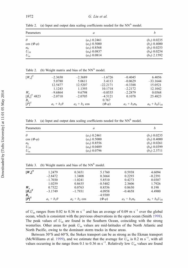
The BP NN models allow us to obtain an empirical equation for the Uss with four inputparameters Uss = f (θ, cos (Φ – φ), σ0, U10). As noted above, a log-sigmoid transferfunction fnet = [1 + exp–x]−1 and linear output function fnet = x are used for the hiddenlayer and output layer for both BP NN models. All four inputs are normalized to between0.1 and 0.9, owing to the asymptotic limits of the hidden-layer transfer function; thescaling coefficients are listed in Table 1. The output empirical equation gives Uss as

Uss ¼ Y � a5ð Þ=b5; (7)

where variable Y is derived as

Y ¼ W yXT þ BT

y (8)

and X is defined as

X ¼ 1þ exp� WXPTþBTX½ �h i�1

: (9)

The subscripts on scaling coefficients (a5 and b5) correspond to the surface oceanStokes drift calculated from the buoy data UA

ss (or USss), where boldface variables are

vectors and superscript T denotes vector transpose. Here, P is a four-row input matrixto the BP NN model transfer function. Equations (7), (8), and (9) provide the BP NNoutputs once they are renormalized using the scaling coefficients in Tables 2 and 3 forNNA and NNS.

3. Global distribution of ocean surface Stokes drift

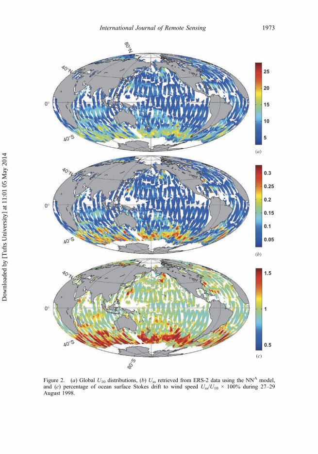
Because the NNA model performs better than the NNS model, we choose this model toretrieve Uss for the global ocean from the ERS-2 scatterometer wind field products (θ, cos(Φ – φ), σ0, U10) for the period 27–29 August 1998, shown in Figure 2(a). During thistime the scatterometer covered the entire oceans of the world just once. The distributionand magnitude of the retrieved Uss are shown in Figure 2(b). We find that the distribution

International Journal of Remote Sensing 1971

Dow

nloa

ded

by [

Tuf

ts U

nive

rsity

] at

11:

01 0

5 M

ay 2

014

of Uss ranges from 0.02 to 0.36 m s−1 and has an average of 0.09 m s−1 over the globalocean, which is consistent with the previous observations in the open ocean (Smith 1998).The peak values of Uss are found in the Southern Ocean, coinciding with the strongwesterlies. Other areas for peak Uss values are mid-latitudes of the North Atlantic andNorth Pacific, owing to the dominant storm tracks in these areas.

Between 30°S and 60°S, the Stokes transport can be as strong as the Ekman transport(McWilliams et al. 1999), and we estimate that the average for Uss is 0.2 m s−1, with allvalues occurring in the range from 0.1 to 0.36 m s−1. Relatively low Uss values are found

Table 2. (a) Input and output data scaling coefficients needed for the NNA model.

Parameters a b

θ (a1) 0.2461 (b1) 0.0235cos (Φ-φ) (a2) 0.5000 (b2) 0.4000σ0 (a3) 0.8568 (b3) 0.0253U10 (a4) 0.0837 (b4) 0.0254Uss (a5) 0.0814 (b5) 2.1592

Table 3. (b) Weight matrix and bias of the NNS model.

[Wx]T 1.2479 0.3651 5.1760 0.5938 4.6094

–2.8472 1.3408 0.3664 0.2293 –0.2391–1.7030 –1.0241 5.8510 0.4273 0.03071.0259 0.8635 –0.5402 2.3606 1.7926

Wy 0.7322 0.0763 0.8556 0.8630 0.198[Bx]

T –3.1749 –1.7931 4.0958 –0.4658 4.4900By –4.9389[P]T a1 + b1θ a2 + b2 cos (Φ-φ) a3 + b3σ0 a4 + b4U10

Table 3. (a) Input and output data scaling coefficients needed for the NNS model.

Parameters a b

θ (a1) 0.2461 (b1) 0.0235cos (Φ-φ) (a2) 0.5000 (b2) 0.4000σ0 (a3) 0.8556 (b3) 0.0261U10 (a4) 0.0489 (b4) 0.0399Uss (a5) 0.0796 (b5) 2.3711

Table 2. (b) Weight matrix and bias of the NNA model.

[Wx]T –2.3650 –2.3689 –1.6726 –0.4045 6.4056

5.0780 5.0611 3.4113 –0.0629 –33.164412.5477 12.5207 –22.2171 –0.3388 15.05211.1243 1.1393 10.1718 –2.2172 12.1042

Wy –9.6864 9.6798 –0.0535 –2.2879 0.0568[Bx]

T 4823 –2.0710 –2.0705 –4.5121 0.1078 25.4823By 0.767[P]T a1 + b1θ a2 + b2 cos (Φ-φ) a3 + b3σ0 a4 + b4U10

1972 G. Liu et al.

Dow

nloa

ded

by [

Tuf

ts U

nive

rsity

] at

11:

01 0

5 M

ay 2

014

25

80°N

40°N

40°N

40°N

0°

0°

0°

40°S

40°S

40°S

80°S

20

15

10

5

(a)

(b)

(c)

0.3

0.25

0.2

0.15

0.1

0.05

1.5

1

0.5

Figure 2. (a) Global U10 distributions, (b) Uss retrieved from ERS-2 data using the NNA model,and (c) percentage of ocean surface Stokes drift to wind speed Uss/U10 × 100% during 27–29August 1998.

International Journal of Remote Sensing 1973

Dow

nloa

ded

by [

Tuf

ts U

nive

rsity

] at

11:

01 0

5 M

ay 2

014

in the tropical and eastern Pacific Ocean and in the tropical Atlantic Ocean, where Uss isgenerally less than 0.09 m s−1 and has an average of 0.05 m s−1. High winds have alsobeen found to correspond to high wave steepness (Liu et al. 2011). Generally, high windsoften induce high wave heights and consequently result in high Uss values. Estimates ofthe percentage of the ocean surface Stokes drift to the wind speed Uss/U10 × 100% areshown in Figure 2(c). The range is from 0.42% to 1.56% with an average of 1.16%.Maximum values are found in areas of high wind speeds in the Southern Ocean wester-lies, where waves are often both fully developed and large, and also in mid-latitudes of theNorth Atlantic and North Pacific regions, related to the dominant storm track areas. SmallStokes drift values are generally found in tropical areas of the eastern Pacific and AtlanticOceans.

4. Scaling Langmuir circulation over the global oceans

4.1. Estimating the Langmuir number

Stokes drift and the associated vortex force are considered to be the possible mechanismsresponsible for the Langmuir circulation (LC) (e.g. Leibovich 1983; McWilliams,Sullivan, and Moeng 1997). Thus, we are motivated to use our newly derived oceansurface Stokes drift and wind stress estimates to characterize this upper ocean phenom-enon. As mentioned above, the vertical mixing induced by Langmuir circulation can reachthe base of the oceanic mixed layer, and the Langmuir circulation often dominates thevelocity field of the ocean mixed layer, which is usually fully turbulent. For surface waveswith a characteristic wavenumber k and Uss, the occurrence of Langmuir circulation inlaminar flow with constant viscosity kv is determined by the Langmuir number La(Leibovich 1977) defined as

La ¼ kvu�

� �32 2u�

Uss

� �12

; (10)

assuming a constant waterside friction velocity u�. This relation represents a balancebetween the rate of diffusion of streamwise vorticity and the rate of production ofstreetwise vorticity by vortex stretching, via the Stokes force.

McWilliams, Sullivan, and Moeng (1997) suggest that the turbulent Langmuir numberLat is the relevant parameter to represent the turbulent oceanic mixed layer and quasi-equilibrium conditions of wind and waves

Lat ¼ u�=Ussð Þ1=2; (11)

because it is indicative of the competition between shear instability of the wind-drivencurrents and the vortex force. We estimated Lat using Equation (11) and u� ¼ τw=ρwð Þ1=2,where τw is the wind stress and τw ¼ CDρaU

210. Here, CD ¼ 0:8þ 0:065� U10ð Þ � 10�3

is the drag coefficient proposed by Wu et al. (1982) and ρw is the density of seawater. Thedistribution of Lat is given in Figure 3(a). Lat is generally in the range from 0.30 to 0.45,which is consistent with observations (e.g. Smith 1992).

It is generally accepted that Langmuir turbulence dominates the TKE energy budget inthe ocean mixed layer when Lat ≤ 0.3. Thus, it is regions such as the Southern Oceanwesterlies and the mid-latitudes storm-tracks corresponding to high Uss that fuel theLangmuir circulation. Transition between Langmuir turbulence and shear turbulence

1974 G. Liu et al.

Dow

nloa

ded

by [

Tuf

ts U

nive

rsity

] at

11:

01 0

5 M

ay 2

014

occurs at 0.5 < Lat < 2 (Grant and Belcher 2009). Therefore, these mid-latitude regions inthe Northern Hemisphere and the tropical Pacific and Atlantic Oceans are where there isintense competition between the shear turbulence and Langmuir turbulence.

4.2. Vertical velocity scale of Langmuir turbulence

Polton and Belcher (2007) analysed Langmuir turbulence in a large eddy simulation(LES) study and argued that within the Stokes layer (where the Stokes drift is dominant),the main competition is between the Stokes production of TKE and dissipation, whenwave breaking is unimportant or absent. Grant and Belcher (2009) also studied the TKEbudget and suggested an approximate velocity scale,

w�L ¼ u2�Uss

� �1=3: (12)

0.42

80°N

40°N

40°N

40°S

40°S

80°S

0°

0.4

0.38

0.36

0.34

0.32

0.3

0.08

0.06

0.04

0.02

(a)

(b)

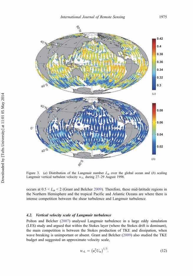
Figure 3. (a) Distribution of the Langmuir number Lat over the global ocean and (b) scalingLangmuir vertical turbulent velocity w�L during 27–29 August 1998.

International Journal of Remote Sensing 1975

Dow

nloa

ded

by [

Tuf

ts U

nive

rsity

] at

11:

01 0

5 M

ay 2

014

Based on Equation (12), we calculated the vertical velocity scale induced by Langmuirturbulence over the global ocean during 27–29 August 1998, as shown in Figure 3(b). Wefound that w�L is as high as 0.1 m s−1 in storm-latitude regions, and also in the westerliesin the Southern Ocean. The average value is 0.02 m s−1. It is clear that high w�L correlateswell with high Uss (Figure 2(b)) and low Lat (Figure 3(a)), whereas low w�L is just theopposite. We estimate that Langmuir turbulence causes dramatic vertical mixing in themixed layer in most of the Southern Ocean, and in some high Uss regions where Langmuirturbulence overwhelms the shear turbulence (Lat < 0.3) and dominates the TKE budget.However, the intensity of the Langmuir turbulence is affected not only by the winds andwaves, but also by the stratification and dynamics of the upper ocean mixed layer, whichare not considered in the present study.

5. Conclusions

Sea state conditions can certainly affect the measurements of wind vectors by scatte-rometer sensors. Moreover, scatterometer backscatter σ0 from the ocean surface canpotentially include sea state information. Whereas previous studies have attempted toexplore the effects of sea state on σ0 for retrievals of wind fields and other variables, inthis study, we explore the relationships between Uss and the ERS-1/2 scatterometersignals. In particular, although it is difficult to measure Stokes drift over the openocean from in situ data, we present a methodology to retrieve Uss from ERS-1/2scatterometer observations, globally. Specifically, we describe a Back-PropagationNeural Network (BP NN) methodology that is applied to retrieve Uss induced byocean waves, and we developed two BP NN models, denoted UA

ss and USss, based on

collocations of in situ buoy data and scatterometer data. This methodology is analternate way to estimate Uss based on remote-sensing data, in conjunction withintegrated wave spectrum parameters estimated from a wave model. In this way, wecalculated Uss over the global ocean during 27–29 August 1998 based on a recentlydeveloped empirical formula for Uss.

The retrieved distribution of Uss ranges from 0.02 to 0.36 m/s and has an average of0.09 m/s over the global ocean. The peak values of Uss correspond to westerlies in theSouthern Ocean and other regions, such as the mid-latitude storm track region where thereare strong winds. Stokes dissipation from ocean wave energy was estimated, assumingthat the wind vector is in the same direction as the surface Stokes drift vector. Fullydeveloped sea state conditions are assumed in order to estimate the wave periods. Duringthe study period, we scaled the Langmuir turbulence to obtain the distributions ofLangmuir number Lat and the associated vertical velocity scale w�L. The Lat distributionsuggests that Langmuir turbulence dominates the energy budget in the westerlies region ofthe Southern Ocean and other high Uss regions, such as those of mid-latitude storm tracks.In addition, strong Langmuir turbulence produces a high-velocity scale within the Stokeslayer.

Thus, we derived global distributions for Uss, and characteristics of the Langmuirturbulence, using scatterometer data. These new results promote a better understanding ofStokes production and its effect on mixing in the ocean mixed layer and the dynamics ofLangmuir circulation. Although this method contains biases, Stokes drift and theLangmuir circulation are essential to the vertical mixing and the transport of materialsand momentum. It is therefore necessary to parameterize these processes in climatestudies, ocean models, and atmosphere–ocean coupled model systems.

1976 G. Liu et al.

Dow

nloa

ded

by [

Tuf

ts U

nive

rsity

] at

11:

01 0

5 M

ay 2

014

AcknowledgementsThanks for the useful suggestions from Jerry Smith from Scripps Institute of Oceanography. Thispaper was supported by the Project from National Natural Science Foundation of China (no.41176159), the Canadian Space Agency GRIP projects ‘Spaceborne Ocean Intelligence Network–SOIN’ and ‘RADARSAT-2 SAR wind retrievals without using external wind direction information’,and PERD (Panel on Energy Research and Development).

ReferencesArdhuin, F., F. Collard, B. Chapron, P. Queffeulou, J.-F. Filipot, and M. Hamon. 2008. “Spectral

Wave Dissipation Based on Observations: A Global Validation.” In Proceedings of the Chinese–German Joint Symposium on Hydraulics & Ocean Engineering, 391–400. Darmstadt: Institutfür Wasserbau und Wasserwirtschaft. www.comc.ncku.edu.tw/joint/joint2008/papers/69.pdf

Ardhuin, F., L. Marié, N. Rascle, P. Forget, and A. Roland. 2009. “Observation of Lagrangian,Stokes and Eulerian Currents Induced by Wind and Waves at the Sea Surface.” Journal ofPhysical Oceanography 39: 2820–2832.

Ardhuin, F., F. R. Martin-lauzer, B. Chapron, P. Craneguy, F. Girard-Ardhuin, and T. Elfouhaily.2004. “Dérive à La Surface de L ’Océan Sous L'Effet des Vagues.” Comptes Rendus Geoscience336: 1121–1130.

Craik, A. D. D., and S. Leibovich. 1976. “A Rational Model for Langmuir Circulations.” Journal ofFluid Mechanics 73: 401–426.

Goodberlet, M. A., and C. T. Swift. 1992. “Improved Retrievals From the DMSP Wind SpeedAlgorithm Under Adverse Weather Conditions.” IEEE Transactions on Geoscience and RemoteSensing 30: 1076–1077.

Grant, A. L. M., and S. E. Belcher. 2009. “Characteristics of Langmuir Turbulence in the OceanMixed Layer.” Journal of Physical Oceanography 39: 1871–1887.

Guo, J., Y. He, X. Chu, L. Cui, and G. Q. Liu. 2009. “Wave Parameters Retrieved from QuikSCATData.” Canadian Journal of Remote Sensing 35: 345–351.

Hanley, K. E., S. E. Belcher, and P. R. Sullivan. 2010. “A Global Climatology of Wind–WaveInteraction.” Journal of Physical Oceanography 40: 1263–1282.

Kantha, L. H., and C. A. Clayson. 2004. “On the Effect of Surface Gravity Waves on Mixing in theOceanic Mixed Layer.” Ocean Modelling 6: 101–124.

Kantha, L. H., P. Wittmann, M. Sclavo, and S. Carniel. 2009. “A Preliminary Estimate of the StokesDissipation of Wave Energy in the Global Ocean.” Geophysical Research Letters 36: L02605.

Keiner, L. E., and X. Yan. 1998. “A Neural Network Model for Estimating Sea Surface Chlorophylland Sediments from Thematic Mapper Imagery.” Remote Sensing of Environment 66: 153–165.

Kenyon, K. E. 1969. “Stokes Drift for Random Gravity Waves.” Journal of Geophysical Research74: 6991–6994.

Krasnopolsky, V. M. 2007. “Neural Network Emulations for Complex MultidimensionalGeophysical Mappings: Applications of Neural Network Techniques to Atmospheric andOceanic Satellite Retrievals and Numerical Modeling.” Reviews of Geophysics 45: RG3009.

Leibovich, S. 1977. “Convective Instability of Stably Stratified Water in the Ocean.” Journal ofFluid Mechanics 82: 561–581.

Leibovich, S. 1980. “On Wave-Current Interaction Theories of Langmuir Circulations.” Journal ofFluid Mechanics 99: 715–724.

Leibovich, S. 1983. “The Form and Dynamics of Langmuir Circulations.” Annual Review of FluidMechanics 15: 391–427.

Li, M., K. Zahariev, and C. Garrett. 1995. “Role of Langmuir Circulation in the Deepening of theOcean Surface Mixed Layer.” Science 270: 1955–1957.

Liu, G. Q., Y. J. He, H. Shen, and J. Guo. 2011. “Global Drag Coefficient Estimates fromScatterometer Wind and Wave Steepness.” IEEE Transactions on Geoscience and RemoteSensing 49: 1499–1503.

McWilliams, J. C., and J. M. Restrepo. 1999. “The Wave-Driven Ocean Circulation.” Journal ofPhysical Oceanography 29: 2523–2540.

McWilliams, J. C., P. P. Sullivan, and C. H. Moeng. 1997. “Langmuir Turbulence in the Ocean.”Journal of Fluid Mechanics 334: 1–30.

International Journal of Remote Sensing 1977

Dow

nloa

ded

by [

Tuf

ts U

nive

rsity

] at

11:

01 0

5 M

ay 2

014

Noh, Y., G. Gahyun, and R. Siegfried. 2011. “Influence of Langmuir Circulation on the Deepeningof the Wind-Mixed Layer.” Journal of Physical Oceanography 41: 472–484.

Polton, J. A., and S. E. Belcher. 2007. “Langmuir Turbulence and Deeply Penetrating Jets in anUnstratified Mixed Layer.” Journal of Geophysical Research 112: C09020.

Quilfen, Y., B. Chapron, F. Collard, and D. Vandemark. 2004. “Relationship between ERSScatterometer Measurement and Integrated Wind and Wave Parameters.” Journal ofAtmospheric and Oceanic Technology 21: 368–373.

Quilfen, Y., B. Chapron, and D. Vandemark. 2001. “The ERS Scatterometer Wind MeasurementAccuracy: Evidence of Seasonal and Regional Biases.” Journal of Atmospheric and OceanicTechnology 18: 1684–1697.

Rascle, N., F. Ardhuin, P. Queffeulou, and D. Croize-Fillon. 2008. “A Global Wave ParameterDatabase for Geophysical Applications. Part 1: Wave-Current-Turbulence InteractionParameters for the Open Ocean Based on Traditional Parameterizations.” Ocean Modelling25: 154–171.

Rascle, N., F. Ardhuin, and E. A. Terry. 2006. “Drift and Mixing Under the Ocean Surface: ACoherent One-Dimensional Description with Application to Unstratified Conditions.” Journalof Geophysical Research 111: C03016.

Sha, W. 2007. “Comments on ‘Water Quality Retrievals From Combined Landsat TM Data andERS-2 SAR Data in the Gulf of Finland.’” IEEE Transactions on Geoscience and RemoteSensing 45: 1896–1897.

Smith, J. 1992. “Observed Growth of Langmuir Circulation.” Journal of Geophysical Research 97:5651–5664.

Smith, J. 1998. “Evolution of Langmuir Circulation During a Storm.” Journal of GeophysicalResearch 103: 12,649–12,668.

Smith, J. A. 1993. “LAI Inversion Using a Back-Propagation Neural Network Trained with aMultiple Scattering Model.” IEEE Transactions on Geoscience and Remote Sensing 31:1102–1106.

Stokes, G. G. 1847. “On the Theory of Oscillatory Waves.” Transactions of the CambridgePhilosophical Society 8: 441–455.

Tamura, H., Y. Miyazawa, and L.-Y. Oey. 2012. “The Stokes Drift and Wave Induced-Mass Flux inthe North Pacific.” Journal of Geophysical Research 117: C08021.

Wu, J. 1982. “Wind-Stress Coefficients over Sea Surface from Breeze to Hurricane.” Journal ofGeophysical Research 87: 9704–9706.

1978 G. Liu et al.

Dow

nloa

ded

by [

Tuf

ts U

nive

rsity

] at

11:

01 0

5 M

ay 2

014