OCEANLYZ Ocean Wave Analyzing Toolbox - Arash … · OCEANLYZ, Ocean Wave Analyzing Toolbox, ... fmaxpcorr maximum frequency for applying pressure attenuation factor ... TMA Spectrum

OCEANLYZ Ocean Wave Analyzing Toolbox

Version 1.3 MATLAB Toolbox

User Manual Arash Karimpour

www.arashkarimpour.com

January, 2015

http://www.arashkarimpour.com/

OCEANLYZ, User Manual

2

Contents License Agreement and Disclaimer ............................................................................................................... 3

Citation .......................................................................................................................................................... 3

Introduction: ................................................................................................................................................. 4

Installation: ................................................................................................................................................... 4

Running: ........................................................................................................................................................ 5

Set up “Run.m”.............................................................................................................................................. 5

Input File: ...................................................................................................................................................... 8

Data recorded in burst mode: ....................................................................................................................... 8

Data recorded in burst mode: ....................................................................................................................... 9

Functions ..................................................................................................................................................... 10

Calculating Wave Parameters Using Spectral Analysis Method (WaveSpectraFun) .................................. 11

Calculating Wave Parameters Using Zero-Crossing Method (WaveZerocrossingFun) ............................... 13

Correcting Wave Pressure Data Using Fast Fourier Transform (PcorFFTFun) ............................................ 14

Correcting Wave Pressure Data Using Linear Wave Theory (PcorZerocrossingFun) .................................. 16

Separating Sea and Swell (SeaSwellFun)..................................................................................................... 17

Sample Files ................................................................................................................................................ 19

Applying Pressure Response Factor ............................................................................................................ 20

Applying Diagnostic Tail .............................................................................................................................. 23

References .................................................................................................................................................. 24


3

License Agreement and Disclaimer This is free software which distributed ONLY for scientific purposes. Series of tests in different conditions have been done to check liability and accuracy of the result, but it is a user responsibility to check the final results for any possible errors. By downloading this package, user agreed that user is responsible for all the outcomes of using this package and developer does not liable and responsible in any way for any problems, shortcomings, errors, and consequences regards of using of this package and its results for any purposes such as design and decision-making process. This software is "AS IS" package, without any kind of warranty and support. The developer is not liable for any type of liability such as claim or damage as a result of the use of this package. Citation Please reference this document as: Karimpour A. (2015), OCEANLYZ, Ocean Wave Analyzing Toolbox, user manual, http://www.arashkarimpour.com/download.html


4

Introduction: OCEANLYZ, Ocean Wave Analyzing Toolbox, is a toolbox for analyzing the wave time series data collected by sensors in open body of water such as ocean, sea, and lake. This toolbox contains functions that each one is suitable for a special purpose. Both spectral and zero-crossing methods are offered for wave analysis. Functions can calculate wave properties such as zero-moment wave height, significant wave height, mean wave height, peak wave period and mean period. This toolbox can correct the pressure attention effect for data selected by the pressure sensor. Sea and swell can be separated and their properties can be reported. Installation: For using this package, after you download it, unzip it in any location you wish. Then open the file named “Run.m” in MATLAB and modify it based on your configuration and requirement. For more information on that, please refer to “Running” section.


5

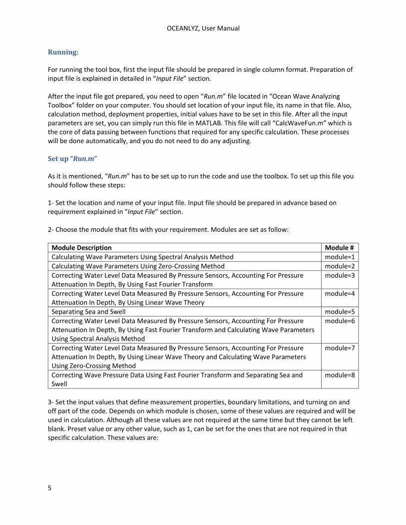
Running: For running the tool box, first the input file should be prepared in single column format. Preparation of input file is explained in detailed in “Input File” section. After the input file got prepared, you need to open “Run.m” file located in “Ocean Wave Analyzing Toolbox” folder on your computer. You should set location of your input file, its name in that file. Also, calculation method, deployment properties, initial values have to be set in this file. After all the input parameters are set, you can simply run this file in MATLAB. This file will call “CalcWaveFun.m” which is the core of data passing between functions that required for any specific calculation. These processes will be done automatically, and you do not need to do any adjusting. Set up “Run.m” As it is mentioned, “Run.m” has to be set up to run the code and use the toolbox. To set up this file you should follow these steps: 1- Set the location and name of your input file. Input file should be prepared in advance based on requirement explained in “Input File” section. 2- Choose the module that fits with your requirement. Modules are set as follow:

Module Description Module #

Calculating Wave Parameters Using Spectral Analysis Method module=1

Calculating Wave Parameters Using Zero-Crossing Method module=2

Correcting Water Level Data Measured By Pressure Sensors, Accounting For Pressure Attenuation In Depth, By Using Fast Fourier Transform

module=3

Correcting Water Level Data Measured By Pressure Sensors, Accounting For Pressure Attenuation In Depth, By Using Linear Wave Theory

module=4

Separating Sea and Swell module=5

Correcting Water Level Data Measured By Pressure Sensors, Accounting For Pressure Attenuation In Depth, By Using Fast Fourier Transform and Calculating Wave Parameters Using Spectral Analysis Method

module=6

Correcting Water Level Data Measured By Pressure Sensors, Accounting For Pressure Attenuation In Depth, By Using Linear Wave Theory and Calculating Wave Parameters Using Zero-Crossing Method

module=7

Correcting Wave Pressure Data Using Fast Fourier Transform and Separating Sea and Swell

module=8

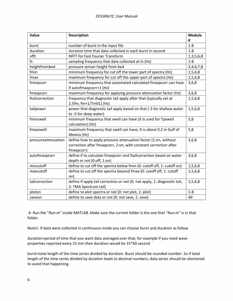
3- Set the input values that define measurement properties, boundary limitations, and turning on and off part of the code. Depends on which module is chosen, some of these values are required and will be used in calculation. Although all these values are not required at the same time but they cannot be left blank. Preset value or any other value, such as 1, can be set for the ones that are not required in that specific calculation. These values are:


6

Value Description Module #

burst number of burst in the input file 1-8

duration duration time that data collected in each burst in second 1-8

nfft NFFT for Fast Fourier Transform 1,3,5,6,8

fs sampling frequency that data collected at in (Hz) 1-8

heightfrombed pressure sensor height from bed 3,4,6,7,8

fmin minimum frequency for cut off the lower part of spectra (Hz) 1,5,6,8

fmax maximum frequency for cut off the upper part of spectra (Hz) 1,5,6,8

fminpcorr minimum frequency that automated calculated fmaxpcorr can have if autofmaxpcorr=1 (Hz)

3,6,8

fmaxpcorr maximum frequency for applying pressure attenuation factor (Hz) 3,6,8

ftailcorrection frequency that diagnostic tail apply after that (typically set at 2.5fm, fm=1/Tm01) (Hz)

1,5,6,8

tailpower power that diagnostic tail apply based on that (-3 for shallow water to -5 for deep water)

1,5,6,8

fminswell minimum frequency that swell can have (it is used for Tpswell calculation) (Hz)

5,8

fmaxswell maximum frequency that swell can have, It is about 0.2 in Gulf of Mexico (Hz)

5,8

pressureattenuation define how to apply pressure attenuation factor (1:on, without correction after fmaxpcorr, 2:on, with constant correction after fmaxpcorr)

3,6,8

autofmaxpcorr define if to calculate fmaxpcorr and ftailcorrection based on water depth or not (0:off, 1:on)

3,6,8

mincutoff define to cut off the spectra below fmin (0: cutoff off, 1: cutoff on) 1,5,6,8

maxcutoff define to cut off the spectra beyond fmax (0: cutoff off, 1: cutoff on)

1,5,6,8

tailcorrection define if apply tail correction or not (0: not apply, 1: diagnostic tail, 2: TMA Spectrum tail)

1,5,6,8

ploton define to plot spectra or not (0: not plot, 1: plot) 1-8

saveon define to save data or not (0: not save, 1: save) All

4- Run the “Run.m” inside MATLAB. Make sure the current folder is the one that “Run.m” is in that folder. Note1: If data were collected in continuous mode you can choose burst and duration as follow duration=period of time that you want data averaged over that, for example if you need wave properties reported every 15 min then duration would be 15*60 second burst=total length of the time series divided by duration. Burst should be rounded number. So if total length of the time series divided by duration leads to decimal numbers, data series should be shortened to avoid that happening.


7

Note2: In the calculation, NFFT value that is set in RUN file will be used. Also, user can set it to be calculated automatically. This should be done inside each function. In that case, NFFT will be set equal to the smallest power of two that is larger than or equal to the absolute value of the total number of data points in each burst. This should be done manually inside that function. Note3: Welch spectrum was used to calculate the spectral power density. In all spectral calculation, Hamming window with segment length of 256 data points and 50% overlap between segments were used. If any other values are required, it should be changed manually inside that function. Note4: autofmaxpcorr=1 will set the software to calculate fmaxpcorr and ftailcorrection based on water depth and sensor height from bed (refer to technical notes). Maximum value for calculated fmaxpcorr and ftailcorrection will be limited to the ones user set in RUN file.


8

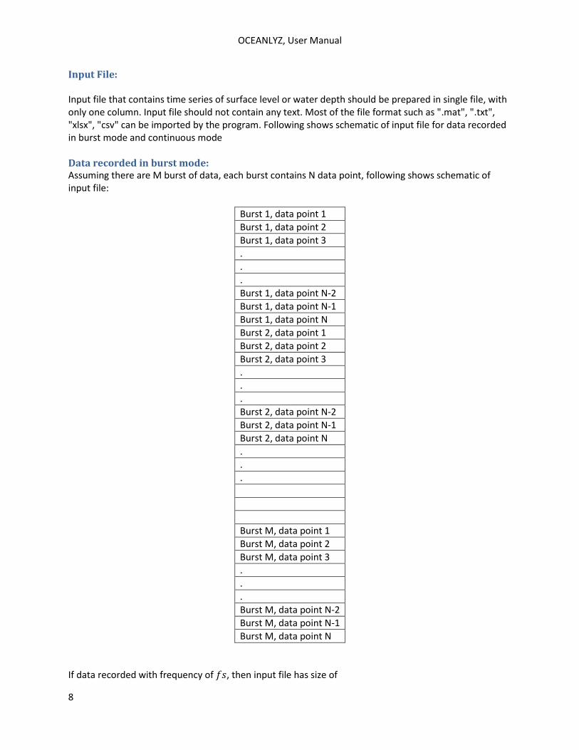
Input File: Input file that contains time series of surface level or water depth should be prepared in single file, with only one column. Input file should not contain any text. Most of the file format such as ".mat", ".txt", "xlsx", "csv" can be imported by the program. Following shows schematic of input file for data recorded in burst mode and continuous mode Data recorded in burst mode: Assuming there are M burst of data, each burst contains N data point, following shows schematic of input file:

Burst 1, data point 1



.

.

.

Burst 1, data point N-2


Burst 1, data point N




.

.

.



Burst 2, data point N

.

.

.

Burst M, data point 1



.

.

.

Burst M, data point N-2

Burst M, data point N-1

Burst M, data point N

If data recorded with frequency of 𝑓𝑠, then input file has size of


9

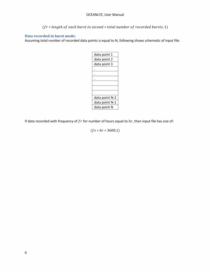
(𝑓𝑟 ∗ 𝑙𝑒𝑛𝑔𝑡ℎ 𝑜𝑓 𝑒𝑎𝑐ℎ 𝑏𝑢𝑟𝑠𝑡 𝑖𝑛 𝑠𝑒𝑐𝑜𝑛𝑑 ∗ 𝑡𝑜𝑡𝑎𝑙 𝑛𝑢𝑚𝑏𝑒𝑟 𝑜𝑓 𝑟𝑒𝑐𝑜𝑟𝑑𝑒𝑑 𝑏𝑢𝑟𝑠𝑡𝑠, 1) Data recorded in burst mode: Assuming total number of recorded data points is equal to N, following shows schematic of input file:

data point 1

data point 2

data point 3

.

.

.

data point N-2

data point N-1

data point N

If data recorded with frequency of 𝑓𝑟 for number of hours equal to ℎ𝑟, then input file has size of:

(𝑓𝑠 ∗ ℎ𝑟 ∗ 3600,1)


10

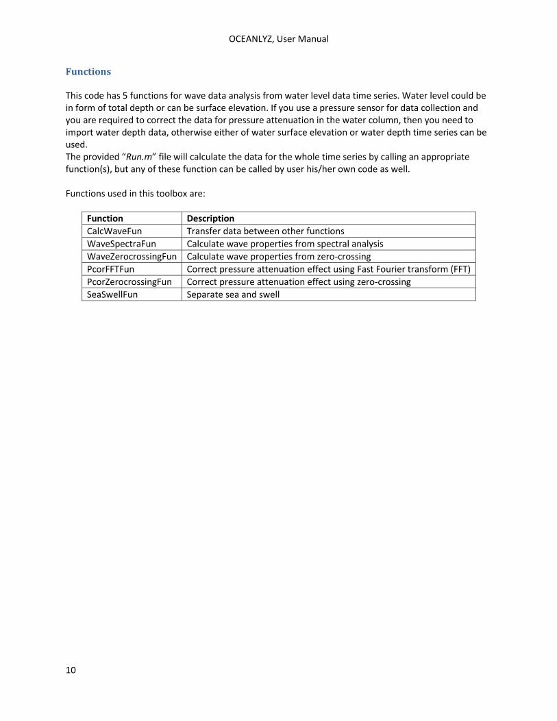
Functions This code has 5 functions for wave data analysis from water level data time series. Water level could be in form of total depth or can be surface elevation. If you use a pressure sensor for data collection and you are required to correct the data for pressure attenuation in the water column, then you need to import water depth data, otherwise either of water surface elevation or water depth time series can be used. The provided “Run.m” file will calculate the data for the whole time series by calling an appropriate function(s), but any of these function can be called by user his/her own code as well. Functions used in this toolbox are:

Function Description

CalcWaveFun Transfer data between other functions

WaveSpectraFun Calculate wave properties from spectral analysis

WaveZerocrossingFun Calculate wave properties from zero-crossing

PcorFFTFun Correct pressure attenuation effect using Fast Fourier transform (FFT)

PcorZerocrossingFun Correct pressure attenuation effect using zero-crossing

SeaSwellFun Separate sea and swell


11

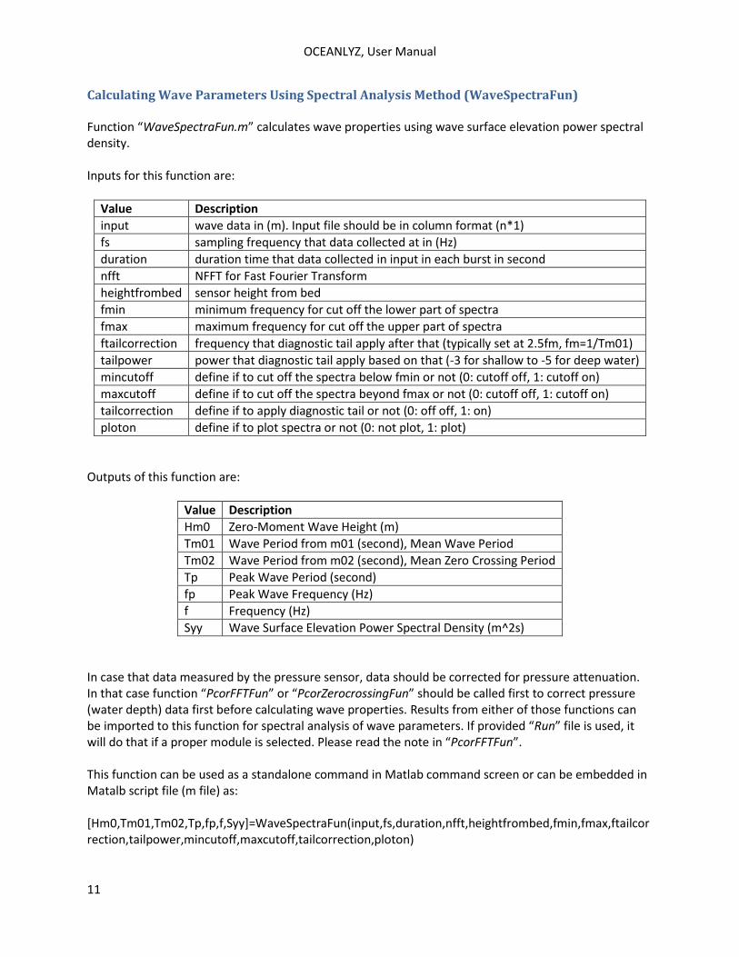
Calculating Wave Parameters Using Spectral Analysis Method (WaveSpectraFun) Function “WaveSpectraFun.m” calculates wave properties using wave surface elevation power spectral density. Inputs for this function are:

Value Description

input wave data in (m). Input file should be in column format (n*1)

fs sampling frequency that data collected at in (Hz)

duration duration time that data collected in input in each burst in second

nfft NFFT for Fast Fourier Transform

heightfrombed sensor height from bed

fmin minimum frequency for cut off the lower part of spectra

fmax maximum frequency for cut off the upper part of spectra

ftailcorrection frequency that diagnostic tail apply after that (typically set at 2.5fm, fm=1/Tm01)

tailpower power that diagnostic tail apply based on that (-3 for shallow to -5 for deep water)

mincutoff define if to cut off the spectra below fmin or not (0: cutoff off, 1: cutoff on)

maxcutoff define if to cut off the spectra beyond fmax or not (0: cutoff off, 1: cutoff on)

tailcorrection define if to apply diagnostic tail or not (0: off off, 1: on)

ploton define if to plot spectra or not (0: not plot, 1: plot)

Outputs of this function are:

Value Description

Hm0 Zero-Moment Wave Height (m)

Tm01 Wave Period from m01 (second), Mean Wave Period

Tm02 Wave Period from m02 (second), Mean Zero Crossing Period

Tp Peak Wave Period (second)

fp Peak Wave Frequency (Hz)

f Frequency (Hz)

Syy Wave Surface Elevation Power Spectral Density (m^2s)

In case that data measured by the pressure sensor, data should be corrected for pressure attenuation. In that case function “PcorFFTFun” or “PcorZerocrossingFun” should be called first to correct pressure (water depth) data first before calculating wave properties. Results from either of those functions can be imported to this function for spectral analysis of wave parameters. If provided “Run” file is used, it will do that if a proper module is selected. Please read the note in “PcorFFTFun”. This function can be used as a standalone command in Matlab command screen or can be embedded in Matalb script file (m file) as: [Hm0,Tm01,Tm02,Tp,fp,f,Syy]=WaveSpectraFun(input,fs,duration,nfft,heightfrombed,fmin,fmax,ftailcorrection,tailpower,mincutoff,maxcutoff,tailcorrection,ploton)


12

Example, using provided sample input file: [Hm0,Tm01,Tm02,Tp,fp,f,Syy]= WaveSpectraFun(input,10,1024,2^10, 0.05,0.04,2,0.9,-4,1,1,0,1);


13

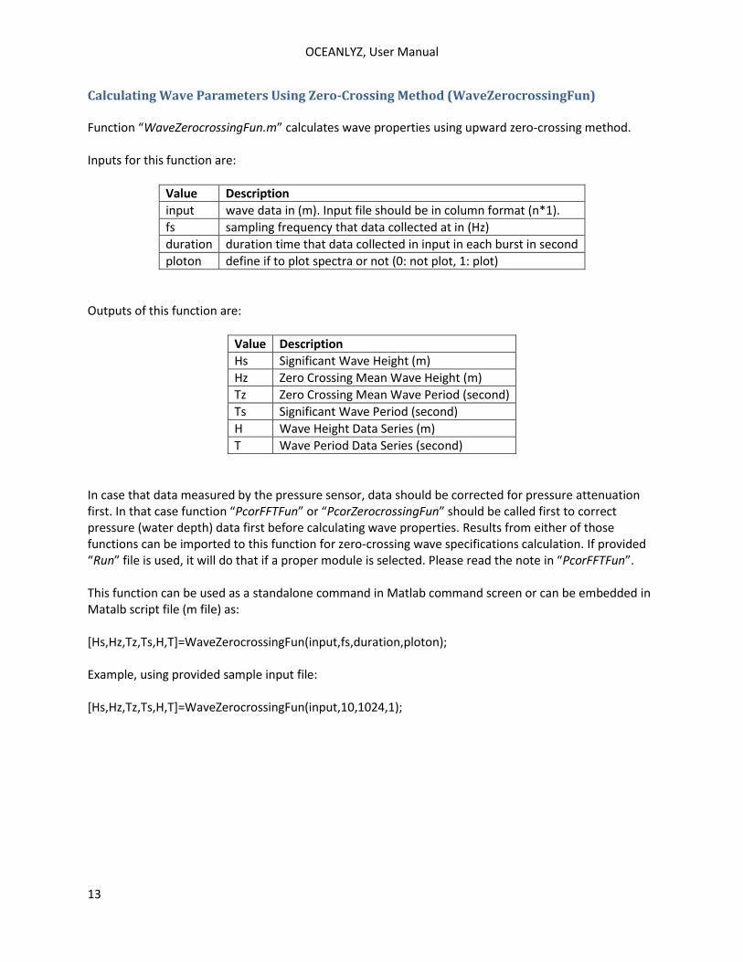
Calculating Wave Parameters Using Zero-Crossing Method (WaveZerocrossingFun) Function “WaveZerocrossingFun.m” calculates wave properties using upward zero-crossing method. Inputs for this function are:

Value Description

input wave data in (m). Input file should be in column format (n*1).





Value Description

Hs Significant Wave Height (m)

Hz Zero Crossing Mean Wave Height (m)

Tz Zero Crossing Mean Wave Period (second)

Ts Significant Wave Period (second)

H Wave Height Data Series (m)

T Wave Period Data Series (second)

In case that data measured by the pressure sensor, data should be corrected for pressure attenuation first. In that case function “PcorFFTFun” or “PcorZerocrossingFun” should be called first to correct pressure (water depth) data first before calculating wave properties. Results from either of those functions can be imported to this function for zero-crossing wave specifications calculation. If provided “Run” file is used, it will do that if a proper module is selected. Please read the note in “PcorFFTFun”. This function can be used as a standalone command in Matlab command screen or can be embedded in Matalb script file (m file) as: [Hs,Hz,Tz,Ts,H,T]=WaveZerocrossingFun(input,fs,duration,ploton); Example, using provided sample input file: [Hs,Hz,Tz,Ts,H,T]=WaveZerocrossingFun(input,10,1024,1);


14

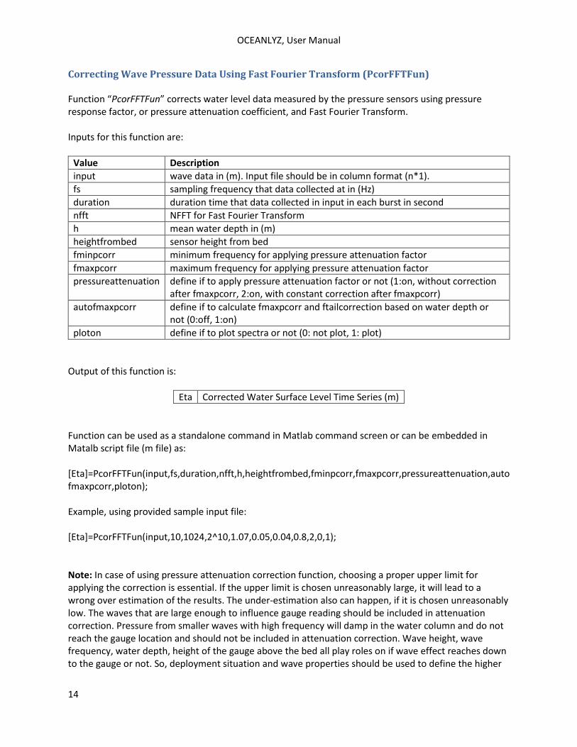
Correcting Wave Pressure Data Using Fast Fourier Transform (PcorFFTFun) Function “PcorFFTFun” corrects water level data measured by the pressure sensors using pressure response factor, or pressure attenuation coefficient, and Fast Fourier Transform. Inputs for this function are:

Value Description





h mean water depth in (m)


fminpcorr minimum frequency for applying pressure attenuation factor

fmaxpcorr maximum frequency for applying pressure attenuation factor

pressureattenuation define if to apply pressure attenuation factor or not (1:on, without correction after fmaxpcorr, 2:on, with constant correction after fmaxpcorr)

autofmaxpcorr define if to calculate fmaxpcorr and ftailcorrection based on water depth or not (0:off, 1:on)


Output of this function is:

Eta Corrected Water Surface Level Time Series (m)

Function can be used as a standalone command in Matlab command screen or can be embedded in Matalb script file (m file) as: [Eta]=PcorFFTFun(input,fs,duration,nfft,h,heightfrombed,fminpcorr,fmaxpcorr,pressureattenuation,autofmaxpcorr,ploton); Example, using provided sample input file: [Eta]=PcorFFTFun(input,10,1024,2^10,1.07,0.05,0.04,0.8,2,0,1); Note: In case of using pressure attenuation correction function, choosing a proper upper limit for applying the correction is essential. If the upper limit is chosen unreasonably large, it will lead to a wrong over estimation of the results. The under-estimation also can happen, if it is chosen unreasonably low. The waves that are large enough to influence gauge reading should be included in attenuation correction. Pressure from smaller waves with high frequency will damp in the water column and do not reach the gauge location and should not be included in attenuation correction. Wave height, wave frequency, water depth, height of the gauge above the bed all play roles on if wave effect reaches down to the gauge or not. So, deployment situation and wave properties should be used to define the higher


15

frequency which has an effect on sensor reading, which pressure correction should not be applied beyond that point.


16

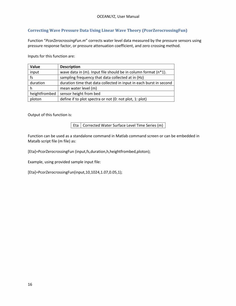
Correcting Wave Pressure Data Using Linear Wave Theory (PcorZerocrossingFun) Function “PcorZerocrossingFun.m” corrects water level data measured by the pressure sensors using pressure response factor, or pressure attenuation coefficient, and zero crossing method. Inputs for this function are:

Value Description




h mean water level (m)



Output of this function is:

Eta Corrected Water Surface Level Time Series (m)

Function can be used as a standalone command in Matlab command screen or can be embedded in Matalb script file (m file) as: [Eta]=PcorZerocrossingFun (input,fs,duration,h,heightfrombed,ploton); Example, using provided sample input file: [Eta]=PcorZerocrossingFun(input,10,1024,1.07,0.05,1);


17

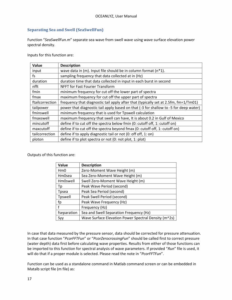
Separating Sea and Swell (SeaSwellFun) Function “SeaSwellFun.m” separate sea wave from swell wave using wave surface elevation power spectral density. Inputs for this function are:

Value Description





fmin minimum frequency for cut off the lower part of spectra

fmax maximum frequency for cut off the upper part of spectra

ftailcorrection frequency that diagnostic tail apply after that (typically set at 2.5fm, fm=1/Tm01)

tailpower power that diagnostic tail apply based on that (-3 for shallow to -5 for deep water)

fminswell minimum frequency that is used for Tpswell calculation

fmaxswell maximum frequency that swell can have, It is about 0.2 in Gulf of Mexico

mincutoff define if to cut off the spectra below fmin (0: cutoff off, 1: cutoff on)

maxcutoff define if to cut off the spectra beyond fmax (0: cutoff off, 1: cutoff on)

tailcorrection define if to apply diagnostic tail or not (0: off off, 1: on)



Value Description

Hm0 Zero-Moment Wave Height (m)

Hm0sea Sea Zero-Moment Wave Height (m)

Hm0swell Swell Zero-Moment Wave Height (m)

Tp Peak Wave Period (second)

Tpsea Peak Sea Period (second)

Tpswell Peak Swell Period (second)

fp Peak Wave Frequency (Hz)

f Frequency (Hz)

fseparation Sea and Swell Separation Frequency (Hz)

Syy Wave Surface Elevation Power Spectral Density (m^2s)

In case that data measured by the pressure sensor, data should be corrected for pressure attenuation. In that case function “PcorFFTFun” or “PcorZerocrossingFun” should be called first to correct pressure (water depth) data first before calculating wave properties. Results from either of those functions can be imported to this function for spectral analysis of wave parameters. If provided “Run” file is used, it will do that if a proper module is selected. Please read the note in “PcorFFTFun”. Function can be used as a standalone command in Matlab command screen or can be embedded in Matalb script file (m file) as:


18

[Hm0,Hm0sea,Hm0swell,Tp,Tpsea,Tpswell,fp,fseparation,f,Syy]=SeaSwellFun(input,fs,duration,nfft,fmin,fmax,ftailcorrection,tailpower,fminswell,fmaxswell,mincutoff,maxcutoff,tailcorrection,ploton); Example, using provided sample input file: [Hm0,Hm0sea,Hm0swell,Tp,Tpswell,fp,fseparation,f,Syy]= SeaSwellFun(input,10,1024,2^10,0.04,2,0.9,-4,0.1,0.25,1,1,0,1);


19

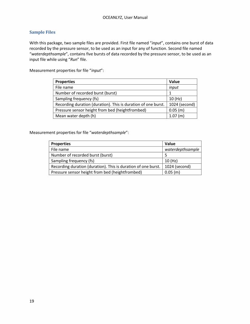
Sample Files With this package, two sample files are provided. First file named “input”, contains one burst of data recorded by the pressure sensor, to be used as an input for any of function. Second file named “waterdepthsample”, contains five bursts of data recorded by the pressure sensor, to be used as an input file while using “Run” file. Measurement properties for file “input”:

Properties Value

File name input

Number of recorded burst (burst) 1

Sampling frequency (fs) 10 (Hz)

Recording duration (duration). This is duration of one burst. 1024 (second)

Pressure sensor height from bed (heightfrombed) 0.05 (m)

Mean water depth (h) 1.07 (m)

Measurement properties for file “waterdepthsample”:

Properties Value

File name waterdepthsample

Number of recorded burst (burst) 5

Sampling frequency (fs) 10 (Hz)

Recording duration (duration). This is duration of one burst. 1024 (second)

Pressure sensor height from bed (heightfrombed) 0.05 (m)


20

Applying Pressure Response Factor Dynamic pressure from wave will attenuate by moving from the water surface toward a bed. Because of that, data collected by the pressure sensor have lower magnitude compared to actual pressure values. To fix this issue, pressure data read by the pressure sensor should be divided by pressure response factor. For that, first pressure data should be converted to water depth as:

ℎ𝑠𝑒𝑛𝑠𝑜𝑟 =𝑃

𝜌𝑔+ 𝑑𝑠

And then, it should be corrected as:

ℎ =ℎ𝑠𝑒𝑛𝑠𝑜𝑟

𝐾𝑃

𝐾𝑃 =cosh 𝑘(𝑑𝑠)

cosh 𝑘ℎ𝑚

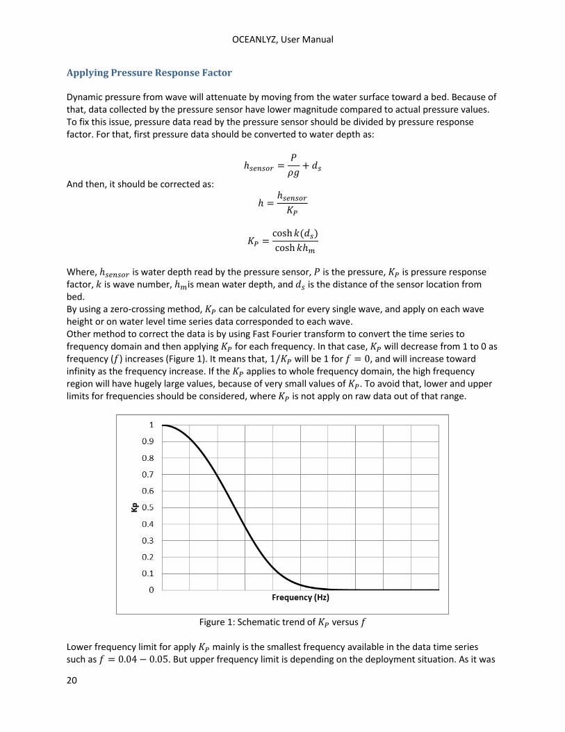
Where, ℎ𝑠𝑒𝑛𝑠𝑜𝑟 is water depth read by the pressure sensor, 𝑃 is the pressure, 𝐾𝑃 is pressure response factor, 𝑘 is wave number, ℎ𝑚is mean water depth, and 𝑑𝑠 is the distance of the sensor location from bed. By using a zero-crossing method, 𝐾𝑃 can be calculated for every single wave, and apply on each wave height or on water level time series data corresponded to each wave. Other method to correct the data is by using Fast Fourier transform to convert the time series to frequency domain and then applying 𝐾𝑃 for each frequency. In that case, 𝐾𝑃 will decrease from 1 to 0 as frequency (𝑓) increases (Figure 1). It means that, 1/𝐾𝑃 will be 1 for 𝑓 = 0, and will increase toward infinity as the frequency increase. If the 𝐾𝑃 applies to whole frequency domain, the high frequency region will have hugely large values, because of very small values of 𝐾𝑃. To avoid that, lower and upper limits for frequencies should be considered, where 𝐾𝑃 is not apply on raw data out of that range.

Figure 1: Schematic trend of 𝐾𝑃 versus 𝑓

Lower frequency limit for apply 𝐾𝑃 mainly is the smallest frequency available in the data time series such as 𝑓 = 0.04 − 0.05. But upper frequency limit is depending on the deployment situation. As it was


21

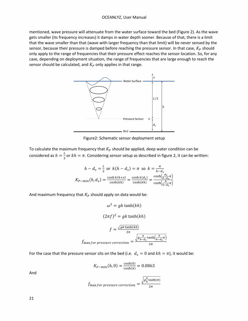
mentioned, wave pressure will attenuate from the water surface toward the bed (Figure 2). As the wave gets smaller (its frequency increases) it damps in water depth sooner. Because of that, there is a limit that the wave smaller than that (wave with larger frequency than that limit) will be never sensed by the sensor, because their pressure is damped before reaching the pressure sensor. In that case, 𝐾𝑃 should only apply to the range of frequencies that their pressure effect reaches the sensor location. So, for any case, depending on deployment situation, the range of frequencies that are large enough to reach the sensor should be calculated, and 𝐾𝑃 only applies in that range.

Figure2: Schematic sensor deployment setup

To calculate the maximum frequency that 𝐾𝑃 should be applied, deep water condition can be

considered as ℎ =𝐿

2 or 𝑘ℎ = 𝜋. Considering sensor setup as described in figure 2, it can be written:

ℎ − 𝑑𝑠 =𝐿

2 or 𝑘(ℎ − 𝑑𝑠) = 𝜋 so 𝑘 =

𝜋

ℎ−𝑑𝑠

𝐾𝑃−𝑚𝑖𝑛(ℎ, 𝑑𝑠) =cosh 𝑘(ℎ+𝑧)

cosh(𝑘ℎ)=

cosh 𝑘(𝑑𝑠)

cosh(𝑘ℎ)=

cosh(𝑑𝑠

ℎ−𝑑𝑠𝜋)

cosh(ℎ

ℎ−𝑑𝑠𝜋)

And maximum frequency that 𝐾𝑃 should apply on data would be:

𝜔2 = 𝑔𝑘 tanh(𝑘ℎ)

(2𝜋𝑓)2 = 𝑔𝑘 tanh(𝑘ℎ)

𝑓 =√𝑔𝑘 tanh(𝑘ℎ)

2𝜋

𝑓max 𝑓𝑜𝑟 𝑝𝑟𝑒𝑠𝑠𝑢𝑟𝑒 𝑐𝑜𝑟𝑟𝑒𝑐𝑡𝑖𝑜𝑛 =√𝑔

𝜋

ℎ−𝑑𝑠tanh(

ℎ

ℎ−𝑑𝑠𝜋)

2𝜋

For the case that the pressure sensor sits on the bed (i.e. 𝑑𝑠 = 0 and 𝑘ℎ = 𝜋), it would be:

𝐾𝑃−𝑚𝑖𝑛(ℎ, 0) =cosh(0)

cosh(𝜋)= 0.0863

And

𝑓max 𝑓𝑜𝑟 𝑝𝑟𝑒𝑠𝑠𝑢𝑟𝑒 𝑐𝑜𝑟𝑟𝑒𝑐𝑡𝑖𝑜𝑛 =√𝑔

𝜋

ℎtanh(𝜋)

2𝜋


22

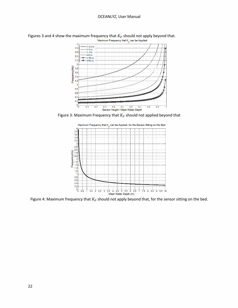
Figures 3 and 4 show the maximum frequency that 𝐾𝑃 should not apply beyond that.

Figure 3: Maximum Frequency that 𝐾𝑃 should not applied beyond that

Figure 4: Maximum frequency that 𝐾𝑃 should not apply beyond that, for the sensor sitting on the bed.


23

Applying Diagnostic Tail Diagnostic is used to correct the high frequency part of the wave spectrum for modeling purpose. It is not recommended to use for measured data, unless data is recorded with low frequency, and no measured data is available for higher frequency, or the noise in higher frequency influence the data. In these cases, higher part of the spectrum can be replaced by diagnostic tail (Siadatmousavi et al. 2012) as:

𝑆𝑦𝑦(𝑓) = 𝑆𝑦𝑦(𝑓𝑡𝑎𝑖𝑙) × (𝑓

𝑓𝑡𝑎𝑖𝑙)

−𝑛 for 𝑓 > 𝑓𝑡𝑎𝑖𝑙

Where 𝑆𝑦𝑦(𝑓) is water surface level power spectrum, 𝑓 is frequency, 𝑓𝑡𝑎𝑖𝑙 is the frequency that tail

applies after that, and 𝑛 is power coefficient. 𝑓𝑡𝑎𝑖𝑙 typically set at 2.5𝑓𝑚 where 𝑓𝑚 = 1/𝑇𝑚01 is a mean frequency (Ardhuin et al. 2010). Value of 𝑛 depends on deployment condition, but typically it is -5 for deep and -3 for shallow water (for more detail refer to literature e.g. Kaihatu et al. 2007, Siadatmousavi et al. 2012).


24

References Ardhuin, F., Rogers, E., Babanin, A. V., Filipot, J. F., Magne, R., Roland, A., ... & Collard, F. (2010). Semiempirical dissipation source functions for ocean waves. Part I: Definition, calibration, and validation. Journal of Physical Oceanography, 40(9), 1917-1941. Kaihatu, J. M., Veeramony, J., Edwards, K. L. & Kirby, J. T. 2007 Asymptotic behaviour of frequency and wave number spectra of nearshore shoaling and breaking waves. J. Geophys. Res. 112, C06016 Siadatmousavi, S. M., Jose, F., & Stone, G. W. (2011). On the importance of high frequency tail in third generation wave models. Coastal Engineering.

Documents

OCEANLYZ Ocean Wave Analyzing Toolbox - Arash … · OCEANLYZ, Ocean Wave Analyzing Toolbox, ... fmaxpcorr maximum frequency for applying pressure attenuation factor ... TMA Spectrum