The interior of dynamical vacuum black holes I:

The C0-stability of the Kerr Cauchy horizon

Mihalis Dafermos∗1 and Jonathan Luk†2

1Department of Mathematics, Princeton University,Washington Road, Princeton NJ 08544, United States of America

1Department of Pure Mathematics and Mathematical Statistics,University of Cambridge, Wilberforce Road, Cambridge CB3 0WB, United Kingdom

2Department of Mathematics, Stanford University,450 Serra Mall Building 380, Stanford CA 94305-2125, United States of America

October 5, 2017

Dedicated to our teacher and mentor Demetrios Christodoulou

Abstract

We initiate a series of works where we study the interior of dynamical rotating vacuum black holeswithout symmetry. In the present paper, we take up the problem starting from appropriate Cauchydata for the Einstein vacuum equations defined on a hypersurface already within the black hole interior,representing the expected geometry just inside the event horizon. We prove that for all such data, themaximal Cauchy evolution can be extended across a non-trivial piece of Cauchy horizon as a Lorentzianmanifold with continuous metric. In subsequent work, we will retrieve our assumptions on data assumingonly that the black hole event horizon geometry suitably asymptotes to a rotating Kerr solution. Inparticular, if the exterior region of the Kerr family is proven to be dynamically stable—as is widelyexpected—then it will follow that the C0-inextendibility formulation of Penrose’s celebrated strong cosmiccensorship conjecture is in fact false. The proof suggests, however, that the C0-metric Cauchy horizonsthus arising are generically singular in an essential way, representing so-called “weak null singularities”,and thus that a revised version of strong cosmic censorship holds.

Contents

1 Introduction 41.1 The Schwarzschild a = 0 case . . . . . . . . . . . . . . . . . . . . . . . . . . . . . . . . . . . . 6

1.1.1 Completeness of I+ and “weak cosmic censorship” . . . . . . . . . . . . . . . . . . . . 61.1.2 The black hole region and the event horizon H+ . . . . . . . . . . . . . . . . . . . . . 71.1.3 Trapped surfaces imply geodesic incompleteness . . . . . . . . . . . . . . . . . . . . . 71.1.4 C0-inextendibility . . . . . . . . . . . . . . . . . . . . . . . . . . . . . . . . . . . . . . 8

1.2 The rotating a 6= 0 Kerr case . . . . . . . . . . . . . . . . . . . . . . . . . . . . . . . . . . . . 91.2.1 Stationary uniqueness and the stability of the exterior . . . . . . . . . . . . . . . . . . 101.2.2 The Cauchy horizon CH+ and the breakdown of determinism . . . . . . . . . . . . . . 111.2.3 The blue-shift instability . . . . . . . . . . . . . . . . . . . . . . . . . . . . . . . . . . . 121.2.4 The C0-formulation of strong cosmic censorship . . . . . . . . . . . . . . . . . . . . . . 121.2.5 Is the finite boundary generically spacelike? . . . . . . . . . . . . . . . . . . . . . . . . 13

∗dafermos@math.princeton.edu†jluk@stanford.edu

1

arX

iv:1

710.

0172

2v1

[gr

-qc]

4 O

ct 2

017

1.3 The main theorems . . . . . . . . . . . . . . . . . . . . . . . . . . . . . . . . . . . . . . . . . . 141.3.1 The evolution of spacelike data and the non-linear C0-stability of the Cauchy horizon 141.3.2 Forthcoming work: event horizon data and the stability of the red-shift region . . . . 141.3.3 Corollary: The C0-formulation of strong cosmic censorship is false . . . . . . . . . . . 151.3.4 Forthcoming work: The C0-stability of the bifurcation sphere of the Cauchy horizon . 15

1.4 Previous work and a reformulation of strong cosmic censorship . . . . . . . . . . . . . . . . . 161.4.1 The linear wave equation on Kerr (and Reissner–Nordstrom) and Christodoulou’s re-

formulation of strong cosmic censorship . . . . . . . . . . . . . . . . . . . . . . . . . . 171.4.2 A non-linear, spherically symmetric toy-model . . . . . . . . . . . . . . . . . . . . . . 221.4.3 Local construction of vacuum weak null singularities without symmetry . . . . . . . . 24

1.5 First remarks on the proof and guide to the paper . . . . . . . . . . . . . . . . . . . . . . . . 251.5.1 The Einstein equations in double null gauge . . . . . . . . . . . . . . . . . . . . . . . . 261.5.2 The bootstrap argument and the logic of the proof . . . . . . . . . . . . . . . . . . . . 271.5.3 The method of [80]: Renormalisation, local weights and null structure . . . . . . . . . 281.5.4 The main estimates . . . . . . . . . . . . . . . . . . . . . . . . . . . . . . . . . . . . . 291.5.5 Auxiliary issues . . . . . . . . . . . . . . . . . . . . . . . . . . . . . . . . . . . . . . . . 321.5.6 The continuity of the extension . . . . . . . . . . . . . . . . . . . . . . . . . . . . . . . 331.5.7 Outline of the paper . . . . . . . . . . . . . . . . . . . . . . . . . . . . . . . . . . . . . 33

1.6 Addendum: the case Λ 6= 0 . . . . . . . . . . . . . . . . . . . . . . . . . . . . . . . . . . . . . 341.7 Acknowledgments . . . . . . . . . . . . . . . . . . . . . . . . . . . . . . . . . . . . . . . . . . . 36

2 Spacetimes covered by double null foliations 362.1 The general class of spacetimes . . . . . . . . . . . . . . . . . . . . . . . . . . . . . . . . . . . 36

2.1.1 The differential structure . . . . . . . . . . . . . . . . . . . . . . . . . . . . . . . . . . 372.1.2 The metric and time-orientation . . . . . . . . . . . . . . . . . . . . . . . . . . . . . . 372.1.3 Frames and metric components . . . . . . . . . . . . . . . . . . . . . . . . . . . . . . . 37

2.2 Geometric interpretation and construction of coordinates . . . . . . . . . . . . . . . . . . . . 382.2.1 The eikonal equation and the double null foliation . . . . . . . . . . . . . . . . . . . . 382.2.2 Construction of double null coordinates . . . . . . . . . . . . . . . . . . . . . . . . . . 38

2.3 Computations . . . . . . . . . . . . . . . . . . . . . . . . . . . . . . . . . . . . . . . . . . . . . 392.3.1 Derivatives and connections . . . . . . . . . . . . . . . . . . . . . . . . . . . . . . . . . 392.3.2 Ricci coefficients and null curvature components . . . . . . . . . . . . . . . . . . . . . 412.3.3 Some basic identities . . . . . . . . . . . . . . . . . . . . . . . . . . . . . . . . . . . . . 42

2.4 Kerr interior in double null foliation . . . . . . . . . . . . . . . . . . . . . . . . . . . . . . . . 43

3 Equations in the double null foliation and the schematic notation 443.1 Equations . . . . . . . . . . . . . . . . . . . . . . . . . . . . . . . . . . . . . . . . . . . . . . . 453.2 Schematic Notation . . . . . . . . . . . . . . . . . . . . . . . . . . . . . . . . . . . . . . . . . . 473.3 Equations in schematic notation . . . . . . . . . . . . . . . . . . . . . . . . . . . . . . . . . . 48

4 Statement of main theorem and the construction of the double null foliation 504.1 Statement of main theorem starting from geometric Cauchy data . . . . . . . . . . . . . . . . 504.2 Setting up a double null foliation . . . . . . . . . . . . . . . . . . . . . . . . . . . . . . . . . . 524.3 Identification with Kerr spacetime and the difference quantities . . . . . . . . . . . . . . . . . 534.4 Initial data for geometric quantities defined with respect to a double null foliation . . . . . . 554.5 Definition of initial data energy with respect to a double null foliation . . . . . . . . . . . . . 584.6 Energies for controlling the solution . . . . . . . . . . . . . . . . . . . . . . . . . . . . . . . . 59

4.6.1 Region of integration . . . . . . . . . . . . . . . . . . . . . . . . . . . . . . . . . . . . . 594.6.2 Conventions for integration . . . . . . . . . . . . . . . . . . . . . . . . . . . . . . . . . 594.6.3 Definitions of the norms . . . . . . . . . . . . . . . . . . . . . . . . . . . . . . . . . . . 594.6.4 Definition of the weight functions . . . . . . . . . . . . . . . . . . . . . . . . . . . . . . 614.6.5 Definition of the energies for the differences of the geometric quantities in (Uuf , g) . . 61

4.7 Statement of main theorem in the double null foliation gauge . . . . . . . . . . . . . . . . . . 644.8 Main bootstrap assumption . . . . . . . . . . . . . . . . . . . . . . . . . . . . . . . . . . . . . 65

2

5 The preliminary estimates 655.1 Sobolev embedding . . . . . . . . . . . . . . . . . . . . . . . . . . . . . . . . . . . . . . . . . . 665.2 General elliptic estimates for elliptic systems . . . . . . . . . . . . . . . . . . . . . . . . . . . 68

6 Estimates for general covariant transport equations 69

7 The reduced schematic equations 777.1 Conventions for the reduced schematic equations . . . . . . . . . . . . . . . . . . . . . . . . . 777.2 Preliminaries . . . . . . . . . . . . . . . . . . . . . . . . . . . . . . . . . . . . . . . . . . . . . 787.3 The inhomogeneous terms . . . . . . . . . . . . . . . . . . . . . . . . . . . . . . . . . . . . . . 867.4 Reduced schematic equations for the difference of the metric components . . . . . . . . . . . 867.5 Reduced schematic null structure equations for the differences of the Ricci coefficients . . . . 897.6 Additional reduced schematic equations for the highest order derivatives of the Ricci coefficients 947.7 Reduced schematic Bianchi equations for the difference of the renormalised null curvature

components . . . . . . . . . . . . . . . . . . . . . . . . . . . . . . . . . . . . . . . . . . . . . . 96

8 The error terms and the main estimate for Nint and Nhyp 99

9 Estimates for the integrated energies via transport equations 1019.1 Preliminary pointwise estimates for the metric components . . . . . . . . . . . . . . . . . . . 1019.2 Estimates for the metric components . . . . . . . . . . . . . . . . . . . . . . . . . . . . . . . . 1049.3 Estimates for the Ricci coefficients . . . . . . . . . . . . . . . . . . . . . . . . . . . . . . . . . 106

10 Energy estimates for the null curvature components 11010.1 First remarks on using (4.27) and Sobolev embedding to control the nonlinear terms . . . . . 111

10.2 Energy estimates for /∇2β, /∇2

K and /∇2˜σ . . . . . . . . . . . . . . . . . . . . . . . . . . . . . 112

10.3 Energy estimates for /∇2K, /∇2˜σ and /∇2

β . . . . . . . . . . . . . . . . . . . . . . . . . . . . . 119

11 Elliptic estimates 124

11.1 Estimates for /∇3η and /∇3

η . . . . . . . . . . . . . . . . . . . . . . . . . . . . . . . . . . . . . 124

11.2 Estimates for /∇3ψH . . . . . . . . . . . . . . . . . . . . . . . . . . . . . . . . . . . . . . . . . 125

11.3 Estimates for /∇3ψH and /∇3

ω . . . . . . . . . . . . . . . . . . . . . . . . . . . . . . . . . . . . 130

11.3.1 Preliminary estimate for /∇ig . . . . . . . . . . . . . . . . . . . . . . . . . . . . . . . . 131

11.3.2 Preliminary estimate for /∇3ω . . . . . . . . . . . . . . . . . . . . . . . . . . . . . . . . 132

11.3.3 Elliptic estimates for /∇3χ . . . . . . . . . . . . . . . . . . . . . . . . . . . . . . . . . . 134

11.3.4 L∞u L2uL

2(S) estimate for /∇3ψH . . . . . . . . . . . . . . . . . . . . . . . . . . . . . . . 135

11.3.5 Estimates for /∇ig, /∇3ω and /∇iη . . . . . . . . . . . . . . . . . . . . . . . . . . . . . . 138

11.3.6 L2uL

2uL

2(S) estimate for /∇3ψH . . . . . . . . . . . . . . . . . . . . . . . . . . . . . . . 138

11.4 Proof of Proposition 8.1 . . . . . . . . . . . . . . . . . . . . . . . . . . . . . . . . . . . . . . . 140

12 Controlling the error terms 14012.1 The Nint,1, Nint,2 and Nhyp,1 energies . . . . . . . . . . . . . . . . . . . . . . . . . . . . . . . 14112.2 Estimates for E1 and E2 . . . . . . . . . . . . . . . . . . . . . . . . . . . . . . . . . . . . . . . 14112.3 Estimates for T1 and T2 . . . . . . . . . . . . . . . . . . . . . . . . . . . . . . . . . . . . . . . 14512.4 Proof of Proposition 12.1 . . . . . . . . . . . . . . . . . . . . . . . . . . . . . . . . . . . . . . 147

13 Recovering the bootstrap assumptions 148

13.1 L1uL∞u L

2(S) estimate for /∇iψH and L1uL∞u L

2(S) estimate for /∇iψH . . . . . . . . . . . . . . 148

13.2 General transport estimates for obtaining L∞u L∞u L

2(S) bounds . . . . . . . . . . . . . . . . . 148

13.3 Main L∞u L∞u L

2(S) estimates . . . . . . . . . . . . . . . . . . . . . . . . . . . . . . . . . . . . 14913.4 Proof of Theorem 4.27 . . . . . . . . . . . . . . . . . . . . . . . . . . . . . . . . . . . . . . . . 154

14 Propagation of higher regularity 154

3

15 Completion of the bootstrap argument 162

16 Continuity of the metric up to the Cauchy horizon 16516.1 The Cauchy horizon CH+ . . . . . . . . . . . . . . . . . . . . . . . . . . . . . . . . . . . . . . 165

16.1.1 Definition of uCH+ and the Cauchy horizon . . . . . . . . . . . . . . . . . . . . . . . . 16516.1.2 Differential structures on U∞ ∪ CH+ . . . . . . . . . . . . . . . . . . . . . . . . . . . . 166

16.2 Additional estimates for /∇4 log Ω . . . . . . . . . . . . . . . . . . . . . . . . . . . . . . . . . . 16716.3 Preliminary continuity estimates . . . . . . . . . . . . . . . . . . . . . . . . . . . . . . . . . . 17116.4 A new coordinate system . . . . . . . . . . . . . . . . . . . . . . . . . . . . . . . . . . . . . . 17516.5 Proof of continuity of the metric . . . . . . . . . . . . . . . . . . . . . . . . . . . . . . . . . . 18216.6 C0-closeness to the Kerr metric . . . . . . . . . . . . . . . . . . . . . . . . . . . . . . . . . . . 18316.7 Conclusion of the proof of Theorem 4.24 . . . . . . . . . . . . . . . . . . . . . . . . . . . . . . 185

17 Relation with weak null singularities 185

A Geometry of Kerr spacetime 188A.1 The Pretorius–Israel coordinate system . . . . . . . . . . . . . . . . . . . . . . . . . . . . . . . 188A.2 Basic estimates on r∗ and θ∗ . . . . . . . . . . . . . . . . . . . . . . . . . . . . . . . . . . . . 190A.3 Estimates for higher derivatives of r and θ as functions of r∗ and θ∗ . . . . . . . . . . . . . . 195A.4 The Kerr metric in double null coordinates . . . . . . . . . . . . . . . . . . . . . . . . . . . . 201A.5 The event horizon and the Cauchy horizon . . . . . . . . . . . . . . . . . . . . . . . . . . . . . 205

A.5.1 Another system of double null coordinates for r close to r+ . . . . . . . . . . . . . . . 205A.5.2 Another system of double null coordinates for r close to r− . . . . . . . . . . . . . . . 206A.5.3 Definition of the event horizon . . . . . . . . . . . . . . . . . . . . . . . . . . . . . . . 206A.5.4 Definition of the Cauchy horizon . . . . . . . . . . . . . . . . . . . . . . . . . . . . . . 206A.5.5 MKerr as a manifold-with-corner . . . . . . . . . . . . . . . . . . . . . . . . . . . . . . 206A.5.6 Metric components in regular coordinates at CH+ . . . . . . . . . . . . . . . . . . . . 207

A.6 Estimates for the Ricci coefficients on Kerr spacetime . . . . . . . . . . . . . . . . . . . . . . 207A.7 Estimates for the null curvature components on Kerr spacetime . . . . . . . . . . . . . . . . . 210A.8 Spacelike hypersurfaces in MKerr . . . . . . . . . . . . . . . . . . . . . . . . . . . . . . . . . 211

1 Introduction

The two-parameter family of Kerr spacetimes (M, ga,M ) [70] constitutes the most celebrated class of explicitsolutions to the Einstein vacuum equations

Ric(g) = 0, (1.1)

the governing equations of general relativity [42] in the absence of matter. The family includes the Schwarz-schild solutions [112] as the non-rotating one-parameter a = 0 subcase. In general, when the rotation param-eter is strictly less than the mass, i.e. |a| < M , the spacetimes (M, ga,M ) contain a black hole region [7, 12],bounded in the past by a null hypersurface H+ known as the event horizon. The Kerr stationary exteriorregion, i.e. the complement of the black hole, is conjectured (see e.g. [31]) to be dynamically stable as asolution of (1.1), under small perturbation of initial data, up to modulation of the parameters. The Kerrexterior geometry is moreover expected to represent the endstate of a wide variety of complicated real-worldastrophysical systems which undergo gravitational collapse [99].

In view of the central role of the Kerr exterior for our current world picture, it is disturbing to recallthat the Kerr black hole region itself, in the strictly rotating case a 6= 0, hides in its interior one of themost difficult conceptual puzzles of general relativity: the dynamical breakdown of classical “Laplacian”determinism for all observers entering the black hole. This breakdown is manifested by the presence of a so-called Cauchy horizon CH+ (see [57]) beyond which Cauchy data no longer uniquely determine the solution.The unsettling nature of this state of affairs has given rise to a conjecture, strong cosmic censorship, firstformulated by Penrose [98], which postulates that the above puzzling behaviour of Kerr is in fact non-generic.This conjecture would imply in particular that the interior region of Kerr must be in some way unstable(under small perturbation of initial data) in the vicinity of its Cauchy horizon CH+. The original formulation

4

Σ

I+ I +H + H

+

CH+

CH +

Σ0

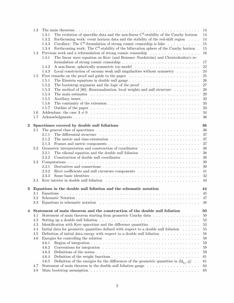
Figure 1: The stability of the Cauchy horizon CH+ from data on Σ0

of the conjecture was modelled on the prototype of the exceptional non-rotating Schwarzschild case a = 0,where no Cauchy horizon is present, but rather, the spacetime can be viewed as terminating at a “spacelikesingularity” across which the metric cannot be extended, even merely continuously [110]. The singularbehaviour of Schwarzschild, though fatal for reckless observers entering the black hole, can be thought ofas epistemologically preferable for general relativity as a theory, since this ensures that the future, howeverbleak, is indeed determined.

We here initiate a series of works to address the stability of the Kerr Cauchy horizon for vacuum space-times governed by (1.1), with no symmetry assumed, and more generally, the question of the nature of theboundary of spacetime in dynamical black hole interiors. The present paper will take up the problem startingfrom general spacelike initial data which are meant to represent a hypersurface Σ0 already in a black holeinterior but close to the event horizon H+ in a suitable sense. For the evolution of such data, the C0-stabilityof a piece of the Kerr Cauchy horizon CH+ will be obtained, contrary to the original expectations motivatedby the Schwarzschild picture. See Figure 1. In a subsequent paper [32], the data considered here will beshown to arise from general characteristic initial data posed on two intersecting null hypersurfaces, one ofwhich is meant to represent the event horizon H+ of a dynamical black hole whose geometry approachesKerr. In a third paper [33], the case of double null data H+

1 ∪ H+2 both hypersurfaces H+

i (i = 1, 2) ofwhich are future complete, globally close to, and asymptote to two nearby Kerr solutions will be considered,and the global C0-stability of the entire bifurcate Cauchy horizon of two-ended Kerr will be obtained. Inparticular, the arising spacetimes will have no spacelike singularities.

Taken together with a future positive resolution of the stability of the exterior of Kerr conjecture, ourresults in particular falsify the C0 formulation of strong cosmic censorship, as well as theoriginal expectation that spacetime generically terminates at a spacelike singularity.

The picture established here of C0-stable Cauchy horizons was in fact first suggested from the detailedstudy of a series of spherically symmetric toy models [64, 102, 93, 10] culminating in the Einstein–Maxwell–scalar field system, for which the analogous result was proven in [26, 27, 29]. For this latter model, it hasbeen proven [82, 83] moreover that, under suitable genericity conditions, the Cauchy horizons that persistinside black holes are singular in an essential sense, and in particular, that the C0 extensions of the metriccannot be C2, in fact, the results strongly suggest that they cannot have locally square integrable Christoffelsymbols (and thus cannot be interpreted even as weak solutions of the Einstein vacuum equations (1.1)).Though in this paper we shall not prove analogues of these instability results in our non-symmetric setting,we note that our theorem is compatible with the statement that for generic initial data for (1.1), the C0-stable Cauchy horizons CH+ will at the same time indeed be singular from the point of view of higherregularity, in precisely the sense suggested by the vacuum “weak null singularities” recently constructedin [80]. (In fact, the expectation that these Cauchy horizons are indeed generically singular in an essentialway is one of the fundamental difficulties of our stability proof, and the methods of [80] will thus play herea paramount role.) For earlier heuristic studies of the relevance of the spherically symmetric toy modelsfor vacuum dynamics without symmetry, see [8, 94, 95]. Thus, our work suggests that an alternative,well-motivated formulation of strong cosmic censorship, originally due to Christodoulou [20],could still hold.

In the remainder of this introduction, we flesh out the above comments with a more detailed discussion,starting in Section 1.1 with a review of the Schwarzschild case and its spacelike singularity. We will thenturn in Section 1.2 to the rotating Kerr case and its smooth Cauchy horizon in the black hole interior,

5

Σ

I+ I +

r = 0

H+H +

Figure 2: Schwarzschild as the maximal future Cauchy development of Σ

formulating both the conjectured stability of the exterior (Conjecture 1) and C0 formulation of strongcosmic censorship (Conjecture 2), which would imply instability of the interior. With this background wewill present in Section 1.3 a first version of the main theorem of the present paper on the C0 stability ofthe Cauchy horizon (Theorem 1), as well as the upcoming results of [32, 33] (Theorems 2 and 3). Inparticular, these theorems together with a positive resolution of Conjecture 1 imply that Conjecture 2 is infact false. In Section 1.4, we will put these theorems in the context of relevant previous work, motivatingthe revised formulation of strong cosmic censorship (Conjecture 3). (For a more detailed discussion ofprevious work, see our survey [34].) Finally, in Section 1.5 we will give a first indication of the proof anda guide to the rest of the paper.

1.1 The Schwarzschild a = 0 case

Any discussion of black holes in general relativity must begin with the simplest example, that of Schwarz-schild [112]. This vacuum solution, discovered already in 1915, sits in the larger Kerr family (M, ga,M ) (tobe reviewed in Section 1.2 below) as the special one-parameter subfamily (M, g0,M ) corresponding to a = 0.The early discovery of Schwarzschild was made possible by its high degree of symmetry. The metric is bothstationary (in fact, static) and spherically symmetric, as is most easily seen from the following explicit formin a coordinate patch:

g0,M = −(1− 2M/r)dt2 + (1− 2M/r)−1dr2 + r2(dθ2 + sin2 θ dφ2). (1.2)

In fact, according to Birkhoff’s theorem [69], all spherically symmetric solutions of (1.1) can be writtenlocally in the form (1.2) for some parameter M ∈ R. In what follows, we shall only consider the case M > 0,whose global geometry will be seen in Section 1.1.2 to indeed contain a black hole region.

The modern interpretation of “the Schwarzschild spacetime” (M, g0,M ) views it as the maximal Cauchydevelopment (see [15]) of vacuum initial data prescribed on an appropriate two-ended asymptotically flathypersurface Σ.1 The spacetime is best illustrated by the Penrose diagram of Figure 2, which depicts—as abounded subset of the plane—the range of a global double null coordinate system U , U . We depict in factonly the maximal future Cauchy development of Σ.2

Astrophysical black holes which arise in gravitational collapse do not have two ends! The potentialphysical relevance of the extended Schwarzschild metric was first exhibited by its connection with theOppenheimer–Snyder model [92] of gravitational collapse of a dust surrounded by vacuum. The latter space-times contain a subset of (M, g0,M ) which can be thought of as the maximal future Cauchy development ofthe hypersurface-with boundary Σ′ depicted in Figure 3. All our statements can be reinterpreted so as torefer only to this region. Nonetheless, it is convenient in the meantime for definiteness to base our discussionon (M, g0,M ) as we have defined it. With reference to Figure 2, we may now review in Sections 1.1.1–1.1.4the features of Schwarzschild geometry relevant for us.

1.1.1 Completeness of I+ and “weak cosmic censorship”

The asymptotic boundary I+ is known as future null infinity and is an idealisation of far away observersin the “radiation zone”. Note that as Σ has two asymptotically flat ends, in our convention I+ has two

1This happens to coincide with the so-called “maximal analytically extended” Schwarzschild spacetime [74, 113], but it isessential here to think of it in terms of the language of the global initial value problem of [15] as a maximal Cauchy development.See the discussion in [34]. The distinction will be fundamental when we turn to Kerr in Section 1.2.

2The specific choice of Σ, so that the bifurcation sphere (see Section 1.1.2 below) lies in its future has simply been made forgreater generality.

6

connected components. A fundamental property that I+ enjoys in Schwarzschild is that of completeness. (Anaive concrete realisation of this is the statement that the spacetime in a neighbourhood of each componentof I+ can be covered by coordinates r, u, θ, φ, related to (1.2) by u = t + r∗(r), with r∗ defined by theequation dr∗

dr = (1− 2M/r), and where u takes on all positive and negative values. See [51] where this issuewas first discussed. For a general definition of what it means for an asymptotically flat vacuum spacetime to“possess a complete future null infinity I+”, see [18].) The completeness of I+ has then the interpretationthat “far-away observers” can observe for all retarded time u. In view of the properties to be discussed inSections 1.1.2–1.1.4 below, this completeness is quite fortuitous!

The conjecture that “for solutions of (1.1) arising from generic asymptotically flat initial data, nullinfinity I+ is complete” is the modern formulation of what is known as weak cosmic censorship. See [18].3

The genericity restriction, not present in the original expectation, was motivated from subsequent work ofChristodoulou [19] on the coupled Einstein–scalar field equations

Ricµν −1

2gµνR = 8πTµν

.= 8π(∂µψ∂νψ −

1

2gµν∂

αψ∂αψ), gψ = 0, (1.3)

under spherical symmetry. In contrast to the vacuum equations (1.1) which are constrained by Birkhoff’stheorem mentioned above, equations (1.3) do admit non-trivial dynamics in spherical symmetry and canbe thought of as one of the simplest toy-models for understanding general dynamics of (1.1) in a 1 + 1dimensional context, in the astrophysically relevant case of one asymptotically flat end. For (1.3) underspherical symmetry, Christodoulou [19] proved the analogue of weak cosmic censorship, but he also showedthat the genericity assumption is indeed necessary via explicit examples of “naked singularities” [17]. Provingweak cosmic censorship for (1.1) without symmetry assumptions is a fundamental open problem in classicalgeneral relativity with potential significance for observational astronomy. It can be thought of as the “globalexistence conjecture” for the Einstein equations. See [20] for this terminology. We will contrast this conjecturewith strong cosmic censorship in Section 1.2.4.

1.1.2 The black hole region and the event horizon H+

The notion of future null infinity I+ allows us to identify the so-called black hole region of (M, g0,M ). Thiscan be characterized as the complement of the past of I+, i.e. M\ J−(I+), and corresponds to the darkershaded region of the Penrose diagram of Figure 2. The interior of the black hole can be represented in theform (1.2) by the range 0 < r < 2M , −∞ < t <∞ (together with standard spherical coordinates θ, φ). Thefuture event horizon H+ (on which r extends smoothly to 2M but the coordinates of (1.2) break down) isa bifurcate future complete null hypersurface separating the black hole region from its exterior4. Note thatthe “stationary” Killing field ∂t in the coordinates of (1.2) is spacelike in the interior of the black hole region.

The constant-(r, t) spheres of the interior of the black hole region are examples of closed trapped sur-faces [100], i.e. both future null expansions are negative. The presence of these trapped surfaces is relatedto the geodesic incompleteness property which we will turn to immediately below.

1.1.3 Trapped surfaces imply geodesic incompleteness

Despite being the Cauchy development of complete, asymptotically flat initial data, the Schwarzschild man-ifold (M, g0,M ) is itself future causally geodesically incomplete. More specifically, timelike geodesics γ arefuture incomplete if and only if they cross H+ into the black hole region; in particular, observers who stayin the exterior J−(I+) live forever (cf. the completeness of I+ discussed in Section 1.1.1).

3The original informal statement of this conjecture, due to Penrose [97], is that “singularities are cloaked by event horizons”.We will discuss the notion of event horizon in Section 1.1.2. The formulation in terms of completeness of future null infinityI+, which is easier to make precise and already captures the essence of the conjecture, originates with [51, 50] and is givena definitive form in [18]. See also [68]. Note of course that to make sense, this formulation must be applied to the maximalCauchy development, not some non-globally hyperbolic extension thereof, cf. the example of negative mass Schwarzschild.See our survey [34]. The conjecture used to be referred to simply as “cosmic censorship”. The term “weak” was added todifferentiate with strong cosmic censorship, discussed in Section 1.2.4, although the modern formulations of these conjecturesare not logically related in the way these adjectives would suggest.

4In our convention, with Σ as depicted, the “exterior” contains a compact subset of the so-called white-hole region M \J+(I−).

7

Σ′

I +

H+

r = 0

Figure 3: The astrophysically relevant maximal future Cauchy development of Σ′

It was originally speculated that the geodesic incompleteness property of Schwarzschild was a result ofits high degree of symmetry [77, 76]. This expectation was spectacularly falsified by Penrose’s celebratedincompleteness5 theorem [100]. This theorem states that a globally hyperbolic spacetime with a non-compactCauchy hypersurface satisfying Ric(v, v) ≥ 0 for all null vectors v is future causally geodesically incompleteif it contains a closed trapped surface. Under additional assumptions of asymptotic flatness, one can alsoinfer that necessarily M\ J−(I+) 6= ∅. Note that by Cauchy stability (see for instance [58]), the existenceof a closed trapped surface in the spacetime is always stable to perturbation of initial data. Applied to themaximal future Cauchy development of vacuum initial data sufficiently close to Schwarzschild data on Σ,this in particular implies that the geodesic incompleteness property of Schwarzschild, as well as the propertythat M\ J−(I+) 6= ∅,6 is stable to perturbation of initial data on Σ.7

1.1.4 C0-inextendibility

What fate awaits incomplete observers γ in the Schwarzschild spacetime? One easily shows that such γasymptote (in finite proper time) to what can be considered as a spacelike8 “singular” boundary of spacetime(“r = 0”), where the curvature (in fact the Kretschmann scalar) blows up asymptotically [58]. This latterproperty is readily computable from the form (1.2). It follows that the manifold (M, g0,M ) is inextendibleas a Lorentzian manifold with C2 metric, i.e. there does not exist a connected 4-dimensional Lorentzianmanifold (M, g) with C2 metric g and an isometric embedding i :M→ M such that i(M) 6= M.

Seen from the PDE perspective, it is not clear that the mere failure of the metric to be C2 is in itselfsufficient to justify interpreting spacetime as having ended at an essential, “terminal” singularity.9 Indeed,the Einstein equations can be shown [71] to be well-posed for general initial data with curvature only inL2. Moreover, explicit solutions with δ-function singularities in curvature on null hypersurfaces have beenconsidered in the physics literature [101], and recently a general well posedness theorem has been provenallowing data with such singular fronts [84]. It turns out, however, that one can say something muchstronger about the singular behaviour of Schwarzschild. Physically speaking, incomplete observers γ notonly measure infinite curvature but are torn apart by infinite tidal deformations as they approach r = 0. Arelated more natural statement is that the spacetime (M, g) is future inextendible as a Lorentzian manifold,in the sense above, but now with metric only assumed to be continuous. This C0-inextendibility property ofSchwarzschild, stated already in [58], has only recently been proven by Sbierski [110].

The prospect of observers being torn apart by infinite tidal deformations may at first seem a ratherunpleasant feature of the Schwarzschild solution. We will see it in a different light, however, after examiningthe situation in the rotating case a 6= 0, where it is precisely the absence of this feature which turns out to beproblematic! The Schwarzschild C0-inextendibility property will then serve as a model for the formulationof strong cosmic censorship reviewed in Section 1.2.4.

5Following [18], we have referred to the result of [100] as an “incompleteness” theorem and not a “singularity” theorem.See again the discussion in [34]. This distinction will be quite clear when the theorem is applied to Kerr (cf. Section 1.2.2).In the Schwarzschild case, geodesic incompleteness of M is indeed related to true “singular” behaviour as will be shown inSection 1.1.4.

6One cannot, however, infer the completeness of I+, cf. Section 1.1.1. Thus weak cosmic censorship is non-trivial even in aneighbourhood of Schwarzschild. See also the statement of Conjecture 1.

7So as not to refer to the two-ended case, note that we could also apply Penrose’s theorem to the maximal Cauchy developmentof small perturbations of complete, one-ended initial data to a suitable Einstein–matter system which are vacuum when restrictedto the subset Σ′ depicted in Figure 3. In this way, the theorem applies to small perturbations away from spherical symmetryof the collapsing dust spacetimes of Oppenheimer–Snyder [92]. The theorem can also be non-trivially applied to the set ofsolutions of Christodoulou’s model [19] which are proven to dynamically form a trapped surface, or, the recent dynamicallyforming trapped surfaces in vacuum [20].

8We will discuss in what sense this boundary can be viewed as spacelike in Section 1.2.5.9For an early discussion of this issue, see the comments in Section 8.4 of [58].

8

Σ

I+ I +

CH+ CH +

H + H+

Figure 4: Kerr as the maximal future Cauchy development of Σ, with a non-unique extension

Σ′

I +

H+

CH +

Figure 5: The astrophysically relevant maximal future Cauchy development of Σ′

1.2 The rotating a 6= 0 Kerr case

The larger two-parameter Kerr family of metrics ga,M in which the one-parameter Schwarzschild subfamilysits was only discovered in 1963 [70]. These metrics retain a stationary Killing field ∂t but, for a 6= 0, onlyone of the generators of spherical symmetry ∂φ; they are thus stationary and axisymmetric. We refer thereader to (A.1) in Appendix A for the form of the Kerr metric in local coordinates and to [91] for a leisurelydiscussion of its geometry. We will only consider the subextremal case 0 ≤ |a| < M .10

In our convention, “the Kerr spacetime” (M, ga,M ) will be the maximal Cauchy development of two-

ended asymptotically flat initial data Σ. This is a proper subset of the maximal analytic extension Mof [7, 12]. Restricting again to the future of Σ, we may illustrate the Kerr spacetime (M, ga,M ) in therotating case a 6= 0 as the two darker shaded regions of the Penrose diagram of Figure 4. Concretely,as in Schwarzschild, we are simply depicting above the range of a global bounded double null coordinatesystem U , U . (The existence of such a global coordinate system is now non-trivial, but was indeed shownby Pretorius–Israel [103]. This type of coordinate system will form the basis of our work in Section 2.) The

significance of the lightest shaded region—not part of (M, g) in our convention but part of (M, g)—willbe discussed in Section 1.2.2 below. The existence of such a smooth extension when a 6= 0 is in completecontrast with the Schwarzschild case.

Before turning to the Kerr black hole interior and its extendibility properties, let us quickly remarksome fundamental similarities with the a = 0 case. The Kerr manifold (M, ga,M ) in the subextremal range|a| < M shares with Schwarzschild all the properties described in Sections 1.1.1–1.1.3, in particular, it has acomplete null infinity I+, a nontrivial black hole region M\ J−(I+), and it is geodesically incomplete. Aswith Schwarzschild, timelike geodesics in (M, ga,M ) are future incomplete if and only if they cross H+.

Though basing our discussion on the Cauchy development (M, ga,M ) of a two-ended hypersurface Σ,just as in the Schwarzschild case, the potentially astrophysically relevant regime is only the future Cauchydevelopment of Σ′ depicted now in Figure 5. The main result of the present paper, Theorem 1, as well as ourupcoming Theorem 2, has an interpretation in terms of this region alone, and it is only the considerationsrelated to Theorem 3 which are intimately connected to the unphysical two-ended picture specifically. Wewill return to this issue at various points in what follows.

The Kerr family of spacetimes should not be viewed as representing merely a particular class of explicitsolutions generalising Schwarzschild. The family can be uniquely characterized by certain properties amongstationary solutions and, in view of this, Kerr is conjectured to play a central role for the dynamics of generalsolutions of (1.1) without symmetry. Thus, various properties of Kerr—if stable!—would have profound

10We note that the dynamics near the extremal case |a| = M are expected to be complicated, see for instance [3]. We willmake some comments regarding extremality at various points further on.

9

(Σ, g, k) ≈ (Σ, ga0,M0 , ka0,M0 )

I+ I +

H +H+

?

g→g a

1,M

1ga

2,M

2←g

Figure 6: The conjectured stability of the Kerr exterior from two-ended data

significance for general relativity. We begin thus with a review of Kerr’s role in the dynamics of (1.1).

1.2.1 Stationary uniqueness and the stability of the exterior

Let us first remark that the sub-extremal Kerr family is known to exhaust all stationary, axisymmetricvacuum exterior spacetimes bounded by a connected non-degenerate event horizon H+ [13, 106]. Moreover,axisymmetry follows from stationarity in the case where the metric is close to Kerr, thus showing that the Kerrfamily is at the very least isolated in the family of stationary, not necessarily axisymmetric, solutions [1]. Thissuggests that it is natural to conjecture the asymptotic stability of the Kerr exterior region under evolutionby (1.1). This is a celebrated conjecture in classical general relativity (see e.g. [31] for background):

Conjecture 1. (Nonlinear stability of the Kerr exterior) Let (Σ, g, k) denote an initial data set for (1.1)suitably close to the induced data of a subextremal Kerr solution with parameters 0 ≤ |a0| < M0. Then themaximal Cauchy development

(a) will possess a complete null infinity I+ (cf. weak cosmic censorship discussed in Section 1.1.1),

(b) will have a black hole exterior region J−(I+) bounded to the future by a smooth future affine completehorizon H+ such that the geometry remains close to ga0,M0 in J−(I+) (See Figure 6) and

(c) will dynamically approach another Kerr metric with nearby parameters 0 ≤ |ai| < Mi, i=1, 2, in eachof the exterior parts J−(I+

i ) corresponding to the two components of null infinity (I+ = I+1 ∪ I

+2 ), in

particular, along H+i , at an inverse polynomial rate. For generic initial data, ai 6= 0, for i = 1, 2.

Thus, according to the above, for small perturbations of Kerr, not only is null infinity I+ still complete(i.e. “weak cosmic censorship” is true restricted to a neighbourhood of Kerr), but the Kerr form of the metricis (asymptotically) stable in the exterior region J−(I+), up to modulation of parameters. We emphasisethat the conjecture makes no statement about the structure of the black hole interior, i.e. the non-emptycomplement M\ J−(I+)! One should compare with the celebrated nonlinear stability of Minkowski spaceR3+1, proven by Christodoulou–Klainerman [21]: There, it is shown that for spacetimes (M, g) arising fromsmall perturbations of trivial initial data, then (a) I+ is complete, (b) M = J−(I+), i.e. there is no blackhole region and the spacetime remains everywhere close to R3+1 and (c) the spacetime asymptotically againsettles down to R3+1 at an at least inverse polynomial rate. Note that in the Kerr case, the statement thatgenerically ai 6= 0, i = 1, 2, simply reflects the expectation that the set of initial data for which the finalparameter ai takes any particular value will be of finite codimension in the set of all data.

We have stated Conjecture 1 for clarity in terms of two-ended initial data. We remark that, in view of atrivial domain of dependence argument, the full content of Conjecture 1 would be captured by statements (a),(b) and (c) restricted to the Cauchy development of Σ′, where I+ has now only one connected component.The situation is depicted in Figure 7. It is the assumption that the boundary of Σ′ is trapped which wouldensure that for sufficiently small perturbations of Kerr data, the new event horizon H+ again lies in thedomain of dependence of Σ′.

It is well known that the assumption of closeness to Kerr in the stationary uniqueness theorem of [1] canbe dropped if one introduces the a priori assumption that the metric is real analytic [58]. Indeed, this wasthe original formulation of the “no-hair” theorem. This analyticity assumption is artificial however becausestationarity does not guarantee that the Killing vector ∂t is timelike everywhere in the exterior, and it isonly in the latter case where analyticity follows from the ellipticity of the reduced equations. (Indeed, inKerr itself with a 6= 0, there is a region outside the black and white holes where ∂t becomes spacelike. Thisis the so-called ergoregion.) If the assumption of analyticity can be replaced by mere smoothness, then the

10

Σ′

I +H+

g→g a,M

Figure 7: The stability of the Kerr exterior localised to the one-ended case

resulting uniqueness property would suggest the more ambitious conjecture that vacuum spacetimes arisingfrom generic asymptotically flat Cauchy data (with one end, and not necessarily initially close to Kerr)will either disperse or settle down to finitely many rotating Kerr black holes moving away from each other.See [99]. According to this then, not only would the Kerr exterior be a stable endstate, but it would be thegeneric endstate of all non-dispersing vacuum solutions.

1.2.2 The Cauchy horizon CH+ and the breakdown of determinism

We now turn to the issue of breakdown of determinism in Kerr. As we have remarked already, the spacetime(M, ga,M ) is smoothly extendible to a larger Lorentzian manifold (M, g), again satisfying the Einstein vacuum

equations (1.1), such that the boundary CH+ of M in M is a bifurcate null hypersurface. Seen from thepoint of view of the global initial value problem [15], however, these extensions are severely non-unique!

What has happened in the above example is a breakdown of global hyperbolicity, the notion first introducedby J. Leray [75] to characterize (for a general class of hyperbolic equations) the region where the domain ofdependence property allows for proofs of uniqueness. The hypersurface Σ is no longer a Cauchy hypersurfacefor M, and this is why data on Σ no longer uniquely determine the solution in M\M, cf. the lightest shadedregion depicted in the Penrose diagram of Figure 4. The null boundary CH+ is thus known as a Cauchyhorizon. This terminology is originally due to Hawking [57].

Kerr in fact exhibits an especially spectacular manifestation of breakdown of determinism in that pre-dictability fails without any local observer directly measuring that the classical regime has been exited.All incomplete observers γ of the original spacetime cross CH+ into the extension M \ M.11 In particu-lar, it is this that justifies our convention, following [18], in referring to Penrose’s theorem of [100] as anincompleteness theorem, and not as a singularity theorem.12

A tempting escape from the epistemological problem of the above breakdown of determinism associatedto the Kerr Cauchy horizon is to appeal to the fact that it is an issue which after all only concerns observersfalling into the black hole. Recall from above that inextendible timelike geodesics γ of Kerr are futureincomplete if and only if they enter M \ J−(I+). The entire future is in particular still determined forobservers “at infinity”, in the sense that I+ is itself complete. Moreover, if “weak cosmic censorship” ofSection 1.1.1 indeed holds, then this latter completeness property is true for the evolution of generic initialdata, i.e. the entire future is safely determined for observers at infinity. Thus, one could ask: Why worryabout the failure of determinism if it only applies to observers who enter black holes?

The above arguments notwithstanding, there is a consensus that such an escape is unsatisfactory. Thequestion of determinism is meant to be an issue of principle. If determinism is indeed a fundamentalproperty of the theory, it should be independent of our choice not to recklessly fall into a black hole. Thus,irrespectively of the validity of “weak cosmic censorship”, the presence of the Kerr Cauchy horizon is generallyconsidered to pose a serious problem for classical general relativity.

11This is in contrast with the Cauchy horizons associated with Christodoulou’s [17] naked singularity solutions of (1.3). Seethe discussion in Section 1.2.4.

12The situation is confused by the fact that the maximal analytic extension (M, g) of [12] happens to itself be incomplete,on account of what can be viewed as “timelike singularities”. There have been several attempts in the literature to formulate

theorems which would imply that any “reasonable” extension of M, not necessarily the analytic M, would still have tobe incomplete. Applying this to some maximal non-globally hyperbolic extension one could infer that there must be localobstructions to extension which could be identified as “singularities”. Indeed, the paper [57], where the terminology “Cauchyhorizon” was introduced, proves precisely such a theorem, followed by [59]. In view of their many assumptions, these theoremsare not, however, very satisfactory. In retrospect, it is precisely identifying the significance of the failure of determinismconnected to Cauchy horizons which appears to be the more fundamental legacy of [57], rather than successfully restoring the“inevitability” of singularity.

11

CH +

A

H+

BI +

Figure 8: The blue-shift instability

1.2.3 The blue-shift instability

It was Penrose again who first identified a key to a promising potential resolution of the conceptual prob-lems generated by Cauchy horizons. He observed [96] that the Kerr Cauchy horizon is associated with aninfinite blue-shift effect depicted in Figure 8. Here, A and B denote the projection of two timelike geodesics(i.e. observers). The wordline of observer A avoids the black hole and has infinite proper length. ObserverB enters the black hole and arrives at the Cauchy horizon in finite proper time. A signal sent by A atconstant frequency will be infinitely shifted to the blue when received by B as B approaches his Cauchyhorizon crossing time.

The above geometric optics effect is indeed manifested as an instability in the behaviour of linear waveequations like the scalar wave equation

gψ = 0 (1.4)

on a fixed Kerr background (M, ga,M ) for a 6= 0. See already Section 1.4.1 for details. Equation (1.4)can in turn be viewed as a naive linearisation of the Einstein vacuum equations (1.1). Thus, this alreadysuggests that perhaps the Kerr Cauchy horizon CH+ is in some sense unstable. Let us emphasise that suchan instability would still be in principle compatible with Conjecture 1, as the latter stability conjecture onlyconcerns the exterior to the black hole.

Of course, linear equations like (1.4) on a fixed globally hyperbolic background can at worst blow upasymptotically (see for instance Chapter 12 of [105]), i.e. exactly at the Cauchy horizon CH+ itself. In thefull non-linear theory, however, governed by (1.1), one might reasonably expect that this instability forcesspacetime to generically break down “before” a Cauchy horizon has the chance to form. This led to thefurther expectation that upon small perturbation, not only is the Cauchy horizon unstable, but the Penrosediagram of the spacetime would revert to the Schwarzschild picture (Figure 2), with a strong spacelikesingularity across which the metric is inextendible as a continuous Lorentzian metric, just as described inSection 1.1.4.

1.2.4 The C0-formulation of strong cosmic censorship

The above considerations regarding the blue-shift allowed Penrose to put forth a general conjecture—nowknown as strong cosmic censorship—which tries to salvage Laplacian determinism for general relativity [98].The gist of this conjecture is that, the Kerr solution notwithstanding, for generic asymptotically flat initialdata, the type of behaviour exhibited in Section 1.2.2 does not arise. There have appeared many differentformulations in the literature over the years; for further discussion see the monograph [41] and our survey [34].One can distill the following mathematical formulation, presented in [20], which captures the spirit of theoriginal expectation of the conjecture:

Conjecture 2 (C0-formulation of strong cosmic censorship). For generic compact or asymptotically flatvacuum initial data, the maximal Cauchy development is inextendible as a Lorentzian manifold with C0

(continuous) metric.

In the language of PDE’s, strong cosmic censorship should be viewed as a statement of global unique-ness.13 The above C0 formulation corresponds precisely with the inextendibility statement that indeed holdsfor Schwarzschild as described in Section 1.1.4, and thus would mean that the maximal Cauchy development

13Cf. the discussion of “weak cosmic censorship” as a statement of “global existence” in Section 1.1.1. We again emphasisethat, with these formulations here, “strong cosmic censorship” is not stronger than “weak cosmic censorship”! See [18] forfurther discussion.

12

is unique in what would appear to be the largest possible reasonable class of spacetimes to consider. Amanifestly weaker formulation which has been considered in the literature replaces C0 with C2 (see [105]).In view of our discussion in Section 1.1.4 above, however, the C2-formulation would fail to capture unique-ness from the perspective of the modern PDE theory of (1.1), for which well-posedness has been proven wellbelow the C2 threshold. We will have to revisit this issue in Section 1.4, after the main results of our paperwill force us to rethink the validity of Conjecture 2.

Let us remark finally that some assumption of compactness or asymptotic flatness in Conjecture 2is clearly necessary in any formulation of strong cosmic censorship, as otherwise there exist trivial, sta-ble examples of Cauchy horizons. For instance, the maximal Cauchy evolution of the Minkowski subsetst = 0 ∩ |r| < 1, and more interestingly, t2 = r2 + 1 ∩ t > 0, are extendible beyond smooth Cauchyhorizons, and this property can be seen to be stable in a suitable sense. One should not think, however,that Cauchy horizons are necessarily associated with non-compactness or other causal pathologies, or nec-essarily hidden inside black holes as in the case of Kerr. Indeed, the examples of naked singularities ofChristodoulou [17], referred to in Section 1.1.1, in addition to exhibiting spacetimes with an incompleteI+, provide examples where spacetime is extendible beyond a Cauchy horizon CH+ such that all p ∈ CH+

correspond to TIPs (see [52] for this terminology) whose past have compact closure with initial data.14 Inshowing the instability of naked singularities for (1.3), Christodoulou has in fact obtained a version of Con-jecture 2 for the system (1.3) under spherical symmetry, together with his proof of weak cosmic censorshipdiscussed in Section 1.1.1. This does not have much bearing, however, for the issue of the stability of theKerr Cauchy horizon, since for Christodoulou’s model, one can show relatively easily that Kerr-like Cauchyhorizons arising from i+ cannot occur under any initial conditions. We will discuss a spherically symmetricmodel generalising (1.3) that does allow for such Kerr-like Cauchy horizons in Section 1.4.2.

1.2.5 Is the finite boundary generically spacelike?

Let us comment explicitly on the other expectation mentioned above connected with strong cosmic censor-ship: the statement that, for generic initial data, the finite boundary of the maximal Cauchy developmentis spacelike.

As in our discussion of Conjecture 2, this expectation can be thought of as being suggested by theSchwarzschild behaviour. One can try to understand this spacelike nature of the boundary canonically inthe sense of TIPs [52]. In that language, the Schwarzschild singularity can indeed be viewed as “spacelike”in the sense that the set of TIPs corresponding to r = 0 have the property that any two are disjointafter intersecting with the future of a sufficiently late Cauchy surface. (Note that this property yieldsmore than the statement that the boundary of the Penrose diagram is spacelike, as the latter suppressesinformation about the angular directions.) For general vacuum Cauchy developments, without symmetry,it is not however straightforward to distinguish a priori the TIPs representing the “finite boundary” fromthe TIPs representing various points at infinity (e.g. from I+). Thus we shall not attempt here a generaldefinition of what it means for the “finite boundary” of spacetime to be spacelike.

Of course, if we happen to know that the maximal Cauchy development (M, g) is indeed extendible

continuously to (M, g), then this gives a direct way of identifying the causal structure of the boundary of

∂M in M. Thus, if Conjecture 2 fails, then we can immediately entertain in this sense the causal propertiesof the part of the finite boundary corresponding to ∂M⊂ M.15 With this, we shall see in the next sectionthat the expectation that the finite boundary is generically spacelike—however one might have hoped toformulate this precisely—will share the same negative fate of Conjecture 2.

14Before the examples of Christodoulou [17], one could imagine that the Kerr-type Cauchy horizons arising from i+ werethe only type of smooth Cauchy horizons which occurred in evolution from smooth asymptotically flat data. This led toformulations of strong cosmic censorship in the literature which did not impose a genericity assumption but focussed only onexcluding completely TIPs whose past had compact closure when intersected with Σ. (See for instance the formulation in thetextbook [115].) Of course, such formulations simply side-step the problem posed by the existence of Kerr, for which a separateconjecture would still have to be formulated. In any case, the examples of [17] would seem to make this a mute point, thoughfor the vacuum equations (1.1), it remains an open problem to construct examples analogous to [17].

15Note that if extensions are suitably regular, then general causality theory and well-posedness already tell us that ∂M⊂ Mis almost everywhere a C1 null hypersurface.

13

CH +

Σ0

g →ga,

M

Figure 9: Stability of CH+ from data on Σ0

CH +

Σ0

H+

Ng−→g a

1,M

1

Figure 10: Stability of CH+ from data on H+ ∪N

1.3 The main theorems

In this paper, we will inaugurate a series of works giving a definitive resolution of the C0-metric stabilityproperties of the Kerr Cauchy horizon. Our results will in particular imply (see Section 1.3.3 below) that, ifthe exterior stability of Kerr (Conjecture 1) is indeed true, then the formulation of strong cosmic censorshipgiven in Section 1.2.4 (Conjecture 2) is in fact false, and moreover, the entire finite boundary of spacetimeis null for all spacetimes arising from data sufficiently near two-ended Kerr data.

1.3.1 The evolution of spacelike data and the non-linear C0-stability of the Cauchy horizon

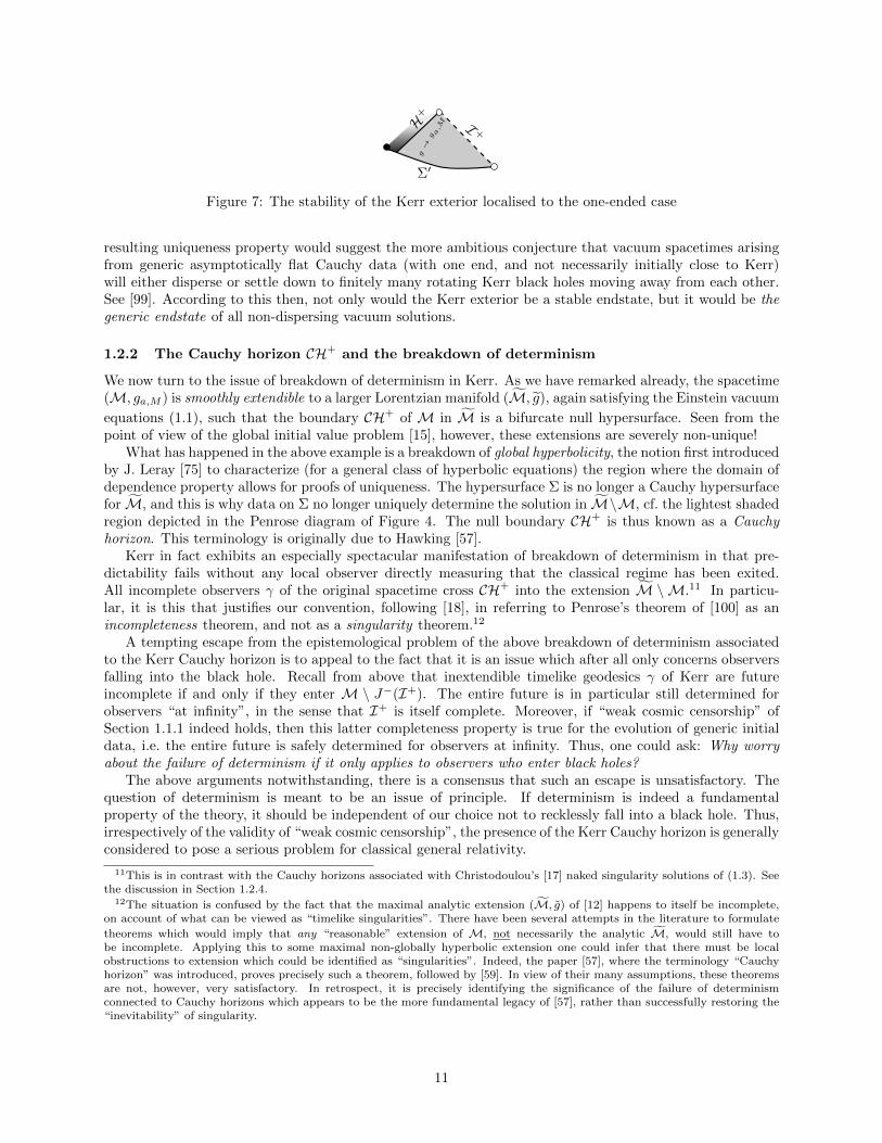
In the present paper, we take up the problem from initial data for (1.1) posed on a hypersurface Σ0 which ismodelled on a Pretorius–Israel u+ u = C hypersurface sandwiched between two constant-r hypersurfaces ofthe Kerr interior with r close to its event horizon value. The assumption on our data is that they asymptoteto induced Kerr data on Σ0, with parameters 0 < |a| < M , at an inverse polynomial rate in u. We thinkof these (see Section 1.3.2 immediately below!) as the “expected induced data” from a general dynamicalvacuum black hole settling down to Kerr, when viewed on a suitably chosen spacelike hypersurface “justinside” the event horizon. The hypersurface is in fact foliated by trapped spheres. The main result of thepresent paper is then the following

Theorem 1. Consider general vacuum initial data corresponding to the expected induced geometry of adynamical black hole settling down to Kerr (with parameters 0 < |a| < M) on a suitable spacelike hypersurfaceΣ0 in the black hole interior. Then the maximal future development spacetime (M, g) corresponding to Σ0

is globally covered by a double null foliation and has a non-trivial Cauchy horizon CH+ across which themetric is continuously extendible.

The domain of the spacetime is depicted in Figure 9. It turns out that we can in fact retrieve ourassumptions on the geometry of Σ0 from an assumption on the event horizon H+ and thus directly relatethem to the stability of Kerr conjecture as formulated in Conjecture 1, as well as to the expectation thatgeneric vacuum spacetimes (not necessarily initially close to Kerr) must either disperse or eventually settledown to a number of Kerr black holes. This event horizon formulation will be the subject of the forthcomingpaper discussed below.

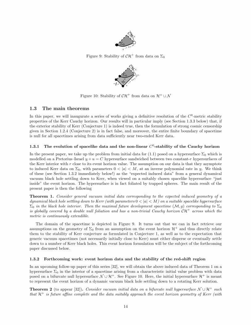
1.3.2 Forthcoming work: event horizon data and the stability of the red-shift region

In an upcoming follow-up paper of this series [32], we will obtain the above induced data of Theorem 1 on ahypersurface Σ0 in the interior of a spacetime arising from a characteristic initial value problem with dataposed on a bifurcate null hypersurface N ∪H+. See Figure 10. Here, the initial hypersurface H+ is meantto represent the event horizon of a dynamic vacuum black hole settling down to a rotating Kerr solution.

Theorem 2 (to appear [32]). Consider vacuum initial data on a bifurcate null hypersurface N ∪H+ suchthat H+ is future affine complete and the data suitably approach the event horizon geometry of Kerr (with

14

Σ

CH +

Σ0

H+

N

g−→ga,M

i+

Figure 11: The C0 formulation of SCC is false!

parameters 0 < |a| < M). Then the maximal future development (M, g) contains a hypersurface Σ0 as inTheorem 1 and thus again has a non-trivial Cauchy horizon CH+ across which the metric is continuouslyextendible.

It follows from the above that any black hole spacetime suitably settling down to a rotating Kerr in itsexterior will have a non-trivial piece of Cauchy horizon. Given the conjectured stability of the Kerr exterior(Conjecture 1), we can already infer a negative result for the C0 formulation of strong cosmic censorship(Conjecture 2). We make this explicit in what follows.

1.3.3 Corollary: The C0-formulation of strong cosmic censorship is false

If the exterior region of Kerr is indeed proven stable up to and including the event horizon H+, it will followthat all spacetimes arising from asymptotically flat initial data sufficiently close to Kerr data on Σ will satisfythe assumptions of Theorem 2, where N is simply taken to be an arbitrary sufficiently short incoming nullhypersurface intersecting H+. A corollary of our results is thus

Corollary. If stability of the Kerr exterior (Conjecture 1) is true, then the Penrose diagram of Kerr is stablenear i+ and the C0-formulation of strong cosmic censorship (Conjecture 2) is false.

The Corollary is depicted in Figure 11. The above statement thus also falsifies the expectation thatgenerically the finite boundary of spacetime is spacelike (cf. Section 1.2.5).

If the more speculative final state picture of [99], described at the end of Section 1.2.1, indeed holds, thenit will follow from Theorem 2 that generic, non-dispersing solutions of the vacuum equations (1.1) arisingfrom asymptotically flat initial data have a metric which is C0-extendible across a piece of a non-empty nullCauchy horizon. In this sense, null finite boundaries of spacetime are ubiquitous in gravitational collapse.

1.3.4 Forthcoming work: The C0-stability of the bifurcation sphere of the Cauchy horizon

For our final forthcoming result, we return to the conclusion of Conjecture 1 as applied specifically in the two-ended case. In that setting, not only does one have a single future-affine complete hypersurface asymptotingto Kerr, but one has in fact a bifurcate future event horizon H+

1 ∪H+2 , both parts of which remain globally

close to a reference Kerr, each moreover asymptoting to two nearby subextremal Kerr’s with parameters ai,Mi, i = 1, 2. Taking such a bifurcate hypersurface as our starting point, we have then the following theorem:

Theorem 3 (to appear [33]). Consider vacuum initial data on a bifurcate null hypersurface H+1 ∪H

+2 , such

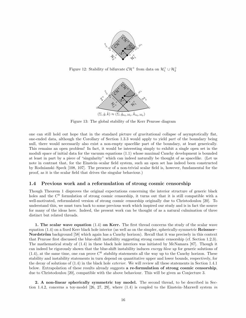
that both hypersurfaces are future complete, and globally close to, and asymptote to Kerr metrics with nearbyparameters 0 < |a1| < M1, and 0 < |a2| < M2, respectively. Then the maximal future development (M, g)can be covered by a double null foliation and moreover can be extended as a C0 metric across a bifurcateCauchy horizon CH+ as depicted in Figure 12. All future-inextendible causal geodesics inM can be extendedto cross CH+.

Thus, if Conjecture 1 is true, then not only is Conjecture 2 false, but the entire Penrose diagram of Kerris stable, up to and including the bifurcation sphere of the Cauchy horizon. See Figure 13. It follows in thiscase that no part of the boundary of spacetime is spacelike, a spectacular failure of the original expectationdescribed in Section 1.2.5.

Of course, the above picture where the entire finite boundary of spacetime consists of a Cauchy horizon(of TIPs with non-compact intersection with initial data) could be an artifice of the two-ended case. Thus,

15

H +2

N

H+

1g−→g a

1,M

1ga2 ,M

2 ←−g

CH+

CH +

Σ0

Figure 12: Stability of bifurcate CH+ from data on H+1 ∪H

+2

N

(Σ, g, k) ≈ (Σ, ga0,M0 , ka0,M0)

I+ I +

H +2 H

+1

CH+

CH +ga2 ,M

2 ←−g g

−→g a

1,M

1

Figure 13: The global stability of the Kerr Penrose diagram

one can still hold out hope that in the standard picture of gravitational collapse of asymptotically flat,one-ended data, although the Corollary of Section 1.3.3 would apply to yield part of the boundary beingnull, there would necessarily also exist a non-empty spacelike part of the boundary, at least generically.This remains an open problem! In fact, it would be interesting simply to exhibit a single open set in themoduli space of initial data for the vacuum equations (1.1) whose maximal Cauchy development is boundedat least in part by a piece of “singularity” which can indeed naturally be thought of as spacelike. (Let usnote in contrast that, for the Einstein–scalar field system, such an open set has indeed been constructedby Rodnianski–Speck [108, 107]. The presence of a non-trivial scalar field is, however, fundamental for theproof, as it is the scalar field that drives the singular behaviour.)

1.4 Previous work and a reformulation of strong cosmic censorship

Though Theorem 1 disproves the original expectations concerning the interior structure of generic blackholes and the C0 formulation of strong cosmic censorship, it turns out that it is still compatible with awell-motivated, reformulated version of strong cosmic censorship originally due to Christodoulou [20]. Tounderstand this, we must turn back to some previous work which inspired our study and is in fact the sourcefor many of the ideas here. Indeed, the present work can be thought of as a natural culmination of threedistinct but related threads.

1. The scalar wave equation (1.4) on Kerr. The first thread concerns the study of the scalar waveequation (1.4) on a fixed Kerr black hole interior (as well as on the simpler, spherically-symmetric Reissner–Nordstrom background [58] which again has a Cauchy horizon). Recall that it was precisely in this contextthat Penrose first discussed the blue-shift instability suggesting strong cosmic censorship (cf. Section 1.2.3).The mathematical study of (1.4) in these black hole interiors was initiated by McNamara [87]. Though itcan indeed be rigorously shown that the blue-shift instability induces energy blow up for generic solutions of(1.4), at the same time, one can prove C0 stability statements all the way up to the Cauchy horizon. Thesestability and instability statements in turn depend on quantitative upper and lower bounds, respectively, forthe decay of solutions of (1.4) in the black hole exterior. We will review all these statements in Section 1.4.1below. Extrapolation of these results already suggests a re-formulation of strong cosmic censorship,due to Christodoulou [20], compatible with the above behaviour. This will be given as Conjecture 3.

2. A non-linear spherically symmetric toy model. The second thread, to be described in Sec-tion 1.4.2, concerns a toy-model [26, 27, 29], where (1.4) is coupled to the Einstein–Maxwell system in

16

spherical symmetry. On the one hand, as a gravitationally coupled non-linear problem, study of this systemgoes beyond the strictly linear setting described in the previous paragraph; on the other hand, it is morerestricted in that it is purely spherically symmetric. This toy-model is itself inspired by even simpler modelproblems considered by Hiscock [64], Poisson–Israel [102], and Ori [93] where the wave equation is replacedby null dust. The toy-model completely vindicates extrapolation of the linear theory of (1.4) describedabove: It has now been proven for the spherically symmetric Einstein–Maxwell–scalar field equations that(i) for all admissible initial data part of the boundary is null and the spacetime extends continuously toa larger spacetime [27, 29] (thus, Conjecture 2 is false for this toy model under spherical symmetry), andthat (ii) for generic initial data in the symmetry class, these null boundaries are singular in a sense to bedescribed [82, 83]; this type of singularity was given the name “weak null singularity”. This gives furtherevidence that Conjecture 3 is the proper formulation of strong cosmic censorship16.

3. Local construction of vacuum weak null singularities without symmetry. The picture of weaknull singularities arising from the above toy model gave rise to much discussion and ongoing debate. At thetime when the spherically symmetric model was first considered, there were no known examples of vacuumspacetimes with null singularities of that type. Thus, one could still even hope that such singular frontsnever occurred for the vacuum equations (1.1). Similarly, one could hope that the weak null singularitiesof [27, 29, 82] would become spacelike when perturbed outside of symmetry. This brings us to the thirdthread, to be discussed in Section 1.4.3. Here, we consider the completely local problem of constructingpatches of vacuum spacetime bounded by “weak null singularities”. A definitive statement was recentlyobtained in [80]. Imposing characteristic initial data with a specific singular profile, one can first showthat a solution exists in a full “rectangular” domain covered by a double null foliation, i.e. no spacelikesingularity immediately arises (stability). Moreover, one can then show a posteriori that the initial singularprofile propagates, naturally inducing a weak null singular boundary on spacetime. This construction can begeneralised from the vacuum equations (1.1) to the Einstein–Maxwell–scalar field equations, the latter nowwithout symmetry. In particular, one can obtain the stability of the weak null singularities of [27, 29, 82] inthe black hole interior, provided that these have already formed.

We turn now in Sections 1.4.1, 1.4.2 and 1.4.3, respectively, to a more detailed discussion of each of theabove threads.

1.4.1 The linear wave equation on Kerr (and Reissner–Nordstrom) and Christodoulou’s re-formulation of strong cosmic censorship

The most basic setting for understanding the stability and instability properties of the Cauchy horizon isthe study of the linear wave equation (1.4) on a fixed Kerr background with initial data defined on Σ.

A simplified setting is the so-called Reissner–Nordstrom background [58]. Recall that the Reissner–Nordstrom family gQ,M is a two parameter family of spherically symmetric metrics which in local coordinatestake the form

gQ,M = −(1− 2M/r +Q2/r2)dt2 + (1− 2M/r +Q2/r2)−1dr2 + r2(dθ2 + sin2 θ dφ2). (1.5)

The metrics are electrovacuum, i.e. together with an appropriate electromagnetic field Fµν they solve theEinstein–Maxwell system

Ricµν −1

2gµνR = 8πTµν

.= 8π(

1

4π(F λµ Fλν −

1

4gµνFαβF

αβ)), (1.6)

∇µFµν = 0, ∇[λFµν] = 0. (1.7)

In the parameter range 0 < |Q| < M , the discussion in Section 1.2 applies equally well to Reissner–Nordstrom, in particular, the form of the Penrose diagram and existence and properties of the Cauchyhorizon. The metric in the region between the event and Cauchy horizon can be expressed as (1.5), where rranges in

M −√M2 −Q2 < r < M +

√M2 −Q2. (1.8)

16though, as we shall see, it is difficult to infer that the most satisfying analogue of Conjecture 3 is true even in this toymodel, in view of the geometric nature of its statement.

17

u=∞

u+ u = C

u=−∞

U=

0

Figure 14: Null coordinates in the black hole interior

Defining r∗ by dr∗

dr = (1−2M/r+Q2/r2)−1, then the region (1.8) is covered by the unbounded null coordinates

u =1

2(r∗ − t), u =

1

2(r∗ + t) (1.9)

as (−∞,∞) × (−∞,∞), with the Cauchy horizon formally parameterised as u = ∞ ∪ u = ∞. SeeFigure 14. The metric can be extended beyond the Cauchy horizon by passing to Kruskal type coordinates:For instance, defining

U = −e−2κ−u, (1.10)

where κ− = r+−r−2r2−

is the surface gravity of the Cauchy horizon, then u =∞ maps to U = 0, and the metric

is seen to be smooth. We will discuss versions of the null coordinates u and u appropriate for non-sphericallysymmetric spacetimes including Kerr in Section 1.5.1. The hypersurface Σ0 corresponds to u+ u = C.

As described in Section 1.2.3, it was precisely in the setting of (1.4) that the blue-shift effect, and itspossible role in allowing for some version of strong cosmic censorship to be true, was originally discussed.Theorem 1.2, to follow shortly below, will indeed provide a rigorous manifestation of the instability associatedwith this effect. What is much less well known, however, is that solutions of the wave equation enjoyglobal C0 stability properties within the black hole interior, still compatible with the blue-shiftinstability. The proof of these interior stability statements is in turn related to quantitative decay estimatesin the exterior, which themselves have only been obtained recently. We turn first to both of these stabilitystatements.

Stability. The study of the wave equation (1.4) on a Kerr background has been the subject of intenseactivity in the past years, and definitive boundedness and decay results, both in the exterior, but, surprisingly,in the interior, have been obtained. The following theorem summarises the statements relevant for us.

Theorem 1.1. Let ψ be a solution of (1.4) on sub-extremal Kerr or Reissner–Nordstrom arising from regularCauchy data on Σ decaying sufficiently fast at spatial infinity.17 Then

1. The solution ψ remains globally bounded in the exterior J−(I+) and decays inverse polynomially to 0,in particular, on the event horizon H+. See [36, 22].

2. The polynomial decay on H+ propagates to similar decay on the spacelike hypersurface Σ0 in the blackhole interior, with respect to coordinates u, u. See [78, 44].

3. The solution ψ is in fact uniformly bounded in all of M, and extends continuously to CH+. See [44,45, 62, 86].

Let us note that the first partial result in the direction of statement 3. was due to McNamara [87], whoessentially showed that 3. held for fixed spherical harmonics ψ` on Reissner–Nordstrom, provided that thescalar field decayed suitably fast on the event horizon, i.e. assuming the analogue of 1., something which atthe time had not been proven. It is interesting that the significance of this stability does not seem to havebeen explicitly noted in most subsequent papers. As we shall see in the discussion below, statement 3. ofthe above theorem can be thought of as the first prototype of our Theorem 1.

17For convenience, one can assume that the data are smooth and compactly supported on Σ, but the result is true undermuch weaker regularity and decay assumptions!

18

The proof of statement 3. depends on obtaining weighted energy estimates for ψ, with appropriate poly-nomial weights in the null coordinates u and u described above. For (1.4), such energy estimates naturallyarise from well-chosen vector fields. Given a vector field V one can associate currents Jµ[ψ] and K[ψ] by

Jµ[ψ] = Tµν [ψ]V µ, K = (V )πµνTµν [ψ] =1

2(LV g)µνTµν [ψ],

where Tµν [ψ] denotes the standard energy momentum tensor18. The wave equation (1.4) implies the diver-gence identity ∫

∇µJµ[ψ] =

∫K[ψ], (1.11)

which upon integration in an appropriate region of the form R = J+(Σ0)∩J−(Σ1) yields an energy identity∫Σ1

Jµ[ψ]nµΣ1+

∫RK[ψ] =

∫Σ0

Jµ[ψ]nµΣ0(1.12)

where integration is always with respect to the induced volume form and nµΣi denotes an appropriate nor-

mal.19

Let us discuss first the Reissner–Nordstrom case. One considers the vector field20

V = r2N (|u|1+2δ∂u + u1+2δ∂u), (1.13)

and applies (1.12) in the region bounded between Σ0 described above and Σ1 = (u = c∪u = c)∩J+(Σ0).The arising flux term

∫Σ1

Jµ[ψ]nµΣ1on the left hand side of (1.12) is positive and controls the following

weighted L2 energies

‖u 12 +δrN∂uψ‖2L2(du sin θdθdφ) + ‖u 1

2 +δΩrN | /∇ψ|‖2L2(du sin θdθdφ), (1.14)

‖|u| 12 +δrN∂uψ‖2L2(du sin θdθdφ) + ‖u 12 +δΩrN | /∇ψ|‖2L2(du sin θdθdφ), (1.15)

where the integrals are taken on u = c∩J+(Σ0) and u = c∩J+(Σ0), respectively. Here | /∇ψ| denotes thenorm of the induced gradient of ψ on the constant-(u, u) spheres of symmetry and Ω2 = −(1−2M/r+Q2/r2).The initial flux on Σ0 appearing on the right hand side of (1.12) is controlled in view of statement 2. ofTheorem 1.1 for sufficiently small δ > 0. Thus, to infer an estimate on (1.14) and (1.15), it remains toexamine the bulk K term in (1.12).

Herein lies the significance of the rN -weight in (1.13). This weight is of course globally bounded aboveand below to the future of Σ0 in view of (1.8), but for N 1, this generates a favourable non-negative partof the “bulk” K-term on the left hand of (1.12),∫

u+u≥C∩u≥c∩u≤cNrN−1[|u|1+2δ(∂uψ)2 + u1+2δ(∂uψ)2] · r2Ω2 sin θ dθ dφ du du (1.16)

which can be used to absorb mixed terms ∂uψ∂uψ also appearing in K, which do not come with a sign.Moreover, quite fortuitously, the only additional terms in K containing angular derivatives come with a goodsign: ∫

u+u≥C∩u≥c∩u≤crN (|u|1+2δ + u1+2δ)‖ /∇ψ|2 · r2Ω2 sin θ dθ dφ du du. (1.17)

Thus, for N 1, the K term is nonnegative, and (1.12) indeed implies a uniform bound for (1.14) and (1.15)from initial data, independent of u ≥ C, u ≤ 0.

18This is defined exactly as in the expression on the right hand side of (1.3).19We will in fact be interested in the case where Σ1 is null; the choice of a volume form again then induces a notion of normal,

which is however tangential to Σ1.20Here the coordinate vector fields are defined with respect to (u, u, θ, φ) coordinates. The argument described here is a

streamlined version of that in [44], where the r-weight and u, u weights were applied in separate regions.

19

Note that along u = c ≤ 0, we may integrate in u1 ≥ u ≥ u0 ≥ C − c to obtain

ψ2(c, u1, θ, φ) .

(∫ u1

u0

∂uψ(c, u, θ, φ)du

)2

+ ψ2(c, u0, θ, φ)

.∫ u1

u0

u−1−2δdu

∫ u1

u0

u1+2δ(∂uψ)2du+ ψ2(c, u0, θ, φ)

. (u−2δ1 − u−2δ

0 )

∫ u1

u0

u1+2δ(∂uψ)2du+ ψ2(c, u0, θ, φ) (1.18)

.∫ u1

u0

u1+2δ(∂uψ)2du+ ψ2(c, u0, θ, φ), (1.19)

where to obtain (1.19) from (1.18) we have used fundamentally that δ > 0. Note that we may apply theabove to WiWjψ in place of ψ, where Wi denote generators of so(3), since the spherical symmetry of (1.5)implies that (1.4) commutes with Wi. Applying the commuted inequality (1.19) with u0 = C− c, so that thesecond term on the right hand side is bounded by data, and integrating further with respect to sin θdθdφ,application of a Sobolev inequality

|ψ|2(u, u, θ, φ) .3∑

i,j=1

∫(|ψ|2 + |WiWjψ|2)(u, u, θ, φ) sin θdθdφ (1.20)

allows one to immediately obtain uniform C0 bounds for ψ from the boundedness of (1.14), giving the firstpart of statement 3. Note that commutation of (1.4) with the Killing field ∂t reveals that ∂tψ is also uniformlybounded. Using this latter fact, the continuous extendibility of ψ to CH+ follows easily by revisiting (1.18)with u0 →∞.

The argument in the Kerr case that statement 2. of Theorem 1.1 implies statement 3. is in fact not muchmore difficult than in Reissner–Nordstrom. One can apply the argument in various coordinates, but forcomparison with the present work, it is most natural to work in a double null foliation of the interior of Kerrdefined by functions u and u, normalised analogously to (1.9) as in Reissner–Nordstrom. This is in fact theapproach of [45]. (We shall review such a foliation in Section 1.5.1.) It is convenient to replace r in (1.13)by a quantity $ which is related to the square root of the area of the constant (u, u)-spheres foliation. Theessential estimate now again follows from the energy identity of the analogue of vector field (1.13). One mustalso deal with the difficulty that the usual commuting in the angular directions now generates error terms.See [62, 86] for alternative approaches.

Instability. We turn now to the blue-shift instability for (1.4).We have already noted the original heuristic considerations of Penrose [96]. It turns out that, together

with the Gaussian beam approximation, the argument of Section 1.2.3 can easily be used to infer that genericfinite-energy solutions on Σ fail to be H1

loc at the Cauchy horizon. See Sbierski [109]. This class of solutionsis too large, however. What we are interested in are solutions which arise from localised initial data on Σ,as in the statement of Theorem 1.1. For such ψ, the decay of waves in the exterior proven as statement 1. ofTheorem 1.1 is a potential counterweight to the blue-shift effect.

Let us discuss first the Reissner–Nordstrom case, where the most definitive results have been obtained:

Theorem 1.2 (L.–Oh [81]). In the Reissner–Nordstrom case, let ψ arise from generic compactly supported21

initial data on Σ. Then

(i) there is a lower bound for the rate of polynomial decay on H+ and

(ii) any non-trivial extension of ψ to an open subset of M fails to be H1loc.

21One can also consider generic data in classes allowing for specific “tails” at spatial infinity.

20

In the above M can be taken to be the standard maximal analytic extension of Reissner–Nordstrom.Note that the failure of ψ to be H1

loc is compatible with the boundedness of (1.14), since if U is the Kruskaltype coordinate (1.10), then the first term of (1.14) transforms to

‖(−U)12 | log(−U)|1/2+δ∂Uψ‖L2(dU sin θdθdφ) (1.21)

which no longer controls ‖∂Uψ‖2L2(dU sin θdθdφ). We will return to the relation between (1.14) and (1.21) inSection 1.5.4, as this will be very relevant for the methods of the present paper.

As we have remarked above, a fundamental difficulty in obtaining instability is that the blue-shift effectis offset by the decay of waves in the exterior. The statement (i) that there is a lower bound on the rate ofdecay on H+ thus turns out to be intimately related to the proof of the H1

loc inextendibility (ii). A strongerlower bound than that of [81] can be obtained by using also the results of [2], and this together with amonotonicity argument of [26] allows one to show that ψ at the Cauchy horizon is not in W 1,p

loc for any p > 1.

An alternative proof of this follows from [54]. Note on the other hand that solutions are indeed in W 1,1loc at

the Cauchy horizon. The special relevance of the space H1loc = W 1,2

loc will become clear below.Turning to Kerr, the failure of ψ to be H1

loc at the Cauchy horizon has been proven in [86], assuming,however, the analogous lower bound on H+ given in Theorem 1.2. It thus remains to obtain the genericityof these lower bounds on H+ to complete the picture.

An alternative approach to obtain a version of Theorem 1.2 in the Kerr case is to construct a suitablesolution from scattering data on past null infinity I−. This approach was pioneered by McNamara [88] andwas completed in [38], using the results of [37]. The result of [38] again yields that the generic localisedsolution on Σ fails to be in H1

loc, but in contrast to Theorem 1.2, it requires working in a class of data slightlylarger than compactly supported functions. Moreover, it does not yield a direct relation between behaviouron H+ and CH+.

Let us note finally that the extremal case |Q| = M or |a| = M hides several subtle surprises both for thestability in the black hole exterior and for the stability and instability questions in the interior. See [3, 48, 49]and the discussion in our survey [34].

Christodoulou’s reformulation of strong cosmic censorship. Were one to naively extrapolate fromthe linear wave equation (1.4) to the non-linear Einstein vacuum equations (1.1), under the identification

g ∼ ψ, Γ ∼ ∂ψ,

then Theorem 1.1 would already suggest the picture of C0-metric stability of our theorems of Section 1.3.Indeed, Theorem 1.1 can be thought of as representing at the same time the analogues of Conjecture 1(statement 1), as well as all three of the main results of this series, Theorems 1–3.

At the same time, naive extrapolation of Theorem 1.2 would suggest that for generic vacuum initial data,the Christoffel symbols Γ would in particular fail to be locally square integrable at the Cauchy horizon. Thesignificance of the Christoffel symbols failing to be in L2

loc is that this implies breakdown even as a weaksolution of the Einstein vacuum equations (1.1). Thus, though not as strong as C0-inextendibility, this notionof inextendibility could still justify viewing the maximal Cauchy development as the unique spacetime whichone can associate with initial data. These considerations motivated Christodoulou to propose the followingreformulation of strong cosmic censorship in his monograph [20]:

Conjecture 3 (Christodoulou re-formulation of strong cosmic censorship [20]). For generic asymptoticallyflat vacuum initial data, the maximal Cauchy development is inextendible as a Lorentzian manifold withcontinuous metric and Christoffel symbols locally square integrable.

With the hindsight of Theorem 1, it is clear that the problem is precisely to show that the naive extrap-olations described above indeed survive in the non-linear theory governed by the Einstein vacuum equations(1.1). Without, however, one might reasonably have thought that given the linear instability of Theorem 1.2,non-linear effects would effectively invalidate the relevance of Theorem 1.1 to the analysis of (1.1) in a neigh-bourhood of the Cauchy horizon. The first evidence to the contrary came from the spherically symmetricnon-linear toy model to be discussed immediately below.

21

1.4.2 A non-linear, spherically symmetric toy-model

We have already remarked that the model (1.3) of Christodoulou does not admit Kerr-like Cauchy horizonsin spherical symmetry. One way to allow for such Cauchy horizons is to add charge to the model, so thatReissner–Nordstrom (1.5) becomes an explicit solution.

The earliest attempts to probe the effects of back-reaction in the context of our problem concernedthe Vaidya model of a self-gravitating, spherically symmetric null dust in the presence of charge, and wereundertaken by Hiscock [64]. A more realistic model considered a spherically symmetric configuration of twonull dusts interacting gravitationally in the presence of charge and was first studied in a seminal work ofPoisson–Israel [102]. For a detailed discussion of these early models, we refer the reader to our survey [34].The most basic truly satisfying toy model, however, is the spherically symmetric Einstein–Maxwell–realscalar field system. Here one couples (1.4) to the Einstein–Maxwell equations (1.6)–(1.7) under sphericalsymmetry, that is to say one considers the evolution of

Ricµν −1

2gµνR = 8πTµν

.= 8π(

1

4π(F λµ Fλν −

1

4gµνFαβF

αβ) + ∂µψ∂νψ −1

2gµν∂

αψ∂αψ), (1.22)

∇µFµν = 0, ∇[λFµν] = 0, gψ = 0, (1.23)

for asymptotically flat spherically symmetric data. If the electromagnetic tensor F is non-trivial, such datanecessarily have two ends, while if F = 0, then the model reduces to the self-gravitating scalar field modelpioneered by Christodoulou [16, 17, 19], mentioned already in Section 1.1.1. We note that the model (1.22)–(1.23) had been discussed heuristically in [6] and studied numerically by [56, 55] and [10, 11], initially withconflicting results.

In the two-ended case, in view of the absence of fixed points for the rotation symmetries, one can easilyshow that, in general, the maximal future Cauchy development of spherically symmetric data will possess acomplete future null infinity I+ with two connected components and a non-empty black hole region, whichwill moreover be bounded in the future by the union CH+ ∪ r = 0, where CH+ = CH+

1 ∪ CH+2 is itself

the union of two possibly empty null boundary components arising from the future endpoints of the eventhorizon. See Figure 15. We have already remarked that in Section 1.2.4, for the model of Christodoulou,i.e. F = 0 in (1.22)–(1.23), one can show easily that CH+ = ∅, while one can show moreover that theboundary r = 0 is spacelike and singular in a suitable sense. This allows one to easily infer a version ofConjecture 2 for Christodoulou’s model in the 2-ended case, without any quantitative understanding of theglobal behaviour of ψ.22 Allowing charge, however, the situation changes completely:

Theorem 1.3. (D. [27, 29], D.–Rodnianski [35]) Let (M, g, Fµν , ψ) be the maximal Cauchy developmentarising from spherically symmetric, admissible23, regular asymptotically flat two-ended initial data for thesystem (1.22)–(1.23). Then the Penrose diagram is as in Figure 15, with I+ complete and H+ non-empty,but with either CH+ or r = 0 possibly empty. The scalar field ψ and its derivatives decay at least inversepolynomially along H+, as well as along a suitable spacelike hypersurface Σ0 in the black hole interior, andthe geometry towards each end approaches a subextremal24 Reissner–Nordstrom 0 ≤ |Q| < Mi. We haveQ = 0 iff Fµν = 0 identically.

If Q = 0 then CH+ = ∅, while if Q 6= 0, then the segments CH+ are necessarily non-empty. Both ψ andthe metric g are continuously extendible beyond CH+.

If the initial data are globally close25 to Reissner–Nordstrom with Q 6= 0, then the boundary r = 0is necessarily empty and CH+ is thus a bifurcate null hypersurface to which g and ψ extend continuously.It follows that the Penrose diagram of Reissner–Nordstrom of Figure 4 is globally stable, and (M, g) is

C0-extendible to (M, g) such that all future incomplete causal geodesics γ pass into M \M.

These results confirmed in particular the numerical studies [10, 11]. A corollary of the above is thefollowing statement

22This is in contrast to the one-ended case, where, as mentioned already in Section 1.2.4, there is an additional (possiblyempty) CH+ segment arising from the centre across which the solution may be extendible. The deep proof [19] of both cosmiccensorship conjectures in the one-ended case amounts to showing that this segment is indeed empty for generic initial data.

23The notion of “admissibility” is a generalisation of the no anti-trapped surfaces condition of Christodoulou, appropriatenow for the two-ended case.

24The sub-extremality can indeed be deduced from the admissibility assumption by an argument of Kommemi. See [82].25Note, in this case, by Cauchy stability one can drop the assumption of “admissibility” and consider Cauchy hypersurfaces

Σ as in Figure 4.

22

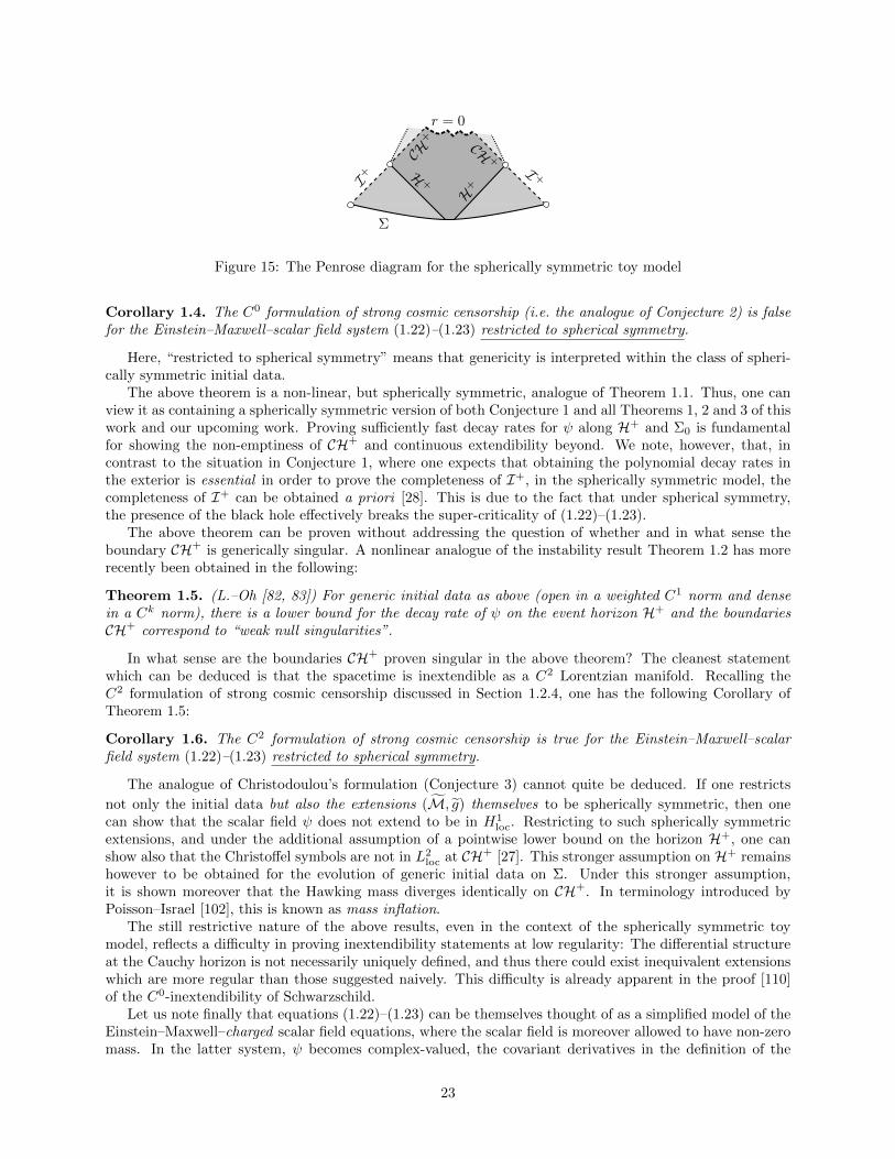
Σ

I +H +

H+

CH+

I+

CH +

r = 0

Figure 15: The Penrose diagram for the spherically symmetric toy model

Corollary 1.4. The C0 formulation of strong cosmic censorship (i.e. the analogue of Conjecture 2) is falsefor the Einstein–Maxwell–scalar field system (1.22)–(1.23) restricted to spherical symmetry.

Here, “restricted to spherical symmetry” means that genericity is interpreted within the class of spheri-cally symmetric initial data.

The above theorem is a non-linear, but spherically symmetric, analogue of Theorem 1.1. Thus, one canview it as containing a spherically symmetric version of both Conjecture 1 and all Theorems 1, 2 and 3 of thiswork and our upcoming work. Proving sufficiently fast decay rates for ψ along H+ and Σ0 is fundamentalfor showing the non-emptiness of CH+ and continuous extendibility beyond. We note, however, that, incontrast to the situation in Conjecture 1, where one expects that obtaining the polynomial decay rates inthe exterior is essential in order to prove the completeness of I+, in the spherically symmetric model, thecompleteness of I+ can be obtained a priori [28]. This is due to the fact that under spherical symmetry,the presence of the black hole effectively breaks the super-criticality of (1.22)–(1.23).

The above theorem can be proven without addressing the question of whether and in what sense theboundary CH+ is generically singular. A nonlinear analogue of the instability result Theorem 1.2 has morerecently been obtained in the following:

Theorem 1.5. (L.–Oh [82, 83]) For generic initial data as above (open in a weighted C1 norm and densein a Ck norm), there is a lower bound for the decay rate of ψ on the event horizon H+ and the boundariesCH+ correspond to “weak null singularities”.

In what sense are the boundaries CH+ proven singular in the above theorem? The cleanest statementwhich can be deduced is that the spacetime is inextendible as a C2 Lorentzian manifold. Recalling theC2 formulation of strong cosmic censorship discussed in Section 1.2.4, one has the following Corollary ofTheorem 1.5:

Corollary 1.6. The C2 formulation of strong cosmic censorship is true for the Einstein–Maxwell–scalarfield system (1.22)–(1.23) restricted to spherical symmetry.

The analogue of Christodoulou’s formulation (Conjecture 3) cannot quite be deduced. If one restricts

not only the initial data but also the extensions (M, g) themselves to be spherically symmetric, then onecan show that the scalar field ψ does not extend to be in H1

loc. Restricting to such spherically symmetricextensions, and under the additional assumption of a pointwise lower bound on the horizon H+, one canshow also that the Christoffel symbols are not in L2

loc at CH+ [27]. This stronger assumption on H+ remainshowever to be obtained for the evolution of generic initial data on Σ. Under this stronger assumption,it is shown moreover that the Hawking mass diverges identically on CH+. In terminology introduced byPoisson–Israel [102], this is known as mass inflation.

The still restrictive nature of the above results, even in the context of the spherically symmetric toymodel, reflects a difficulty in proving inextendibility statements at low regularity: The differential structureat the Cauchy horizon is not necessarily uniquely defined, and thus there could exist inequivalent extensionswhich are more regular than those suggested naively. This difficulty is already apparent in the proof [110]of the C0-inextendibility of Schwarzschild.

Let us note finally that equations (1.22)–(1.23) can be themselves thought of as a simplified model of theEinstein–Maxwell–charged scalar field equations, where the scalar field is moreover allowed to have non-zeromass. In the latter system, ψ becomes complex-valued, the covariant derivatives in the definition of the

23

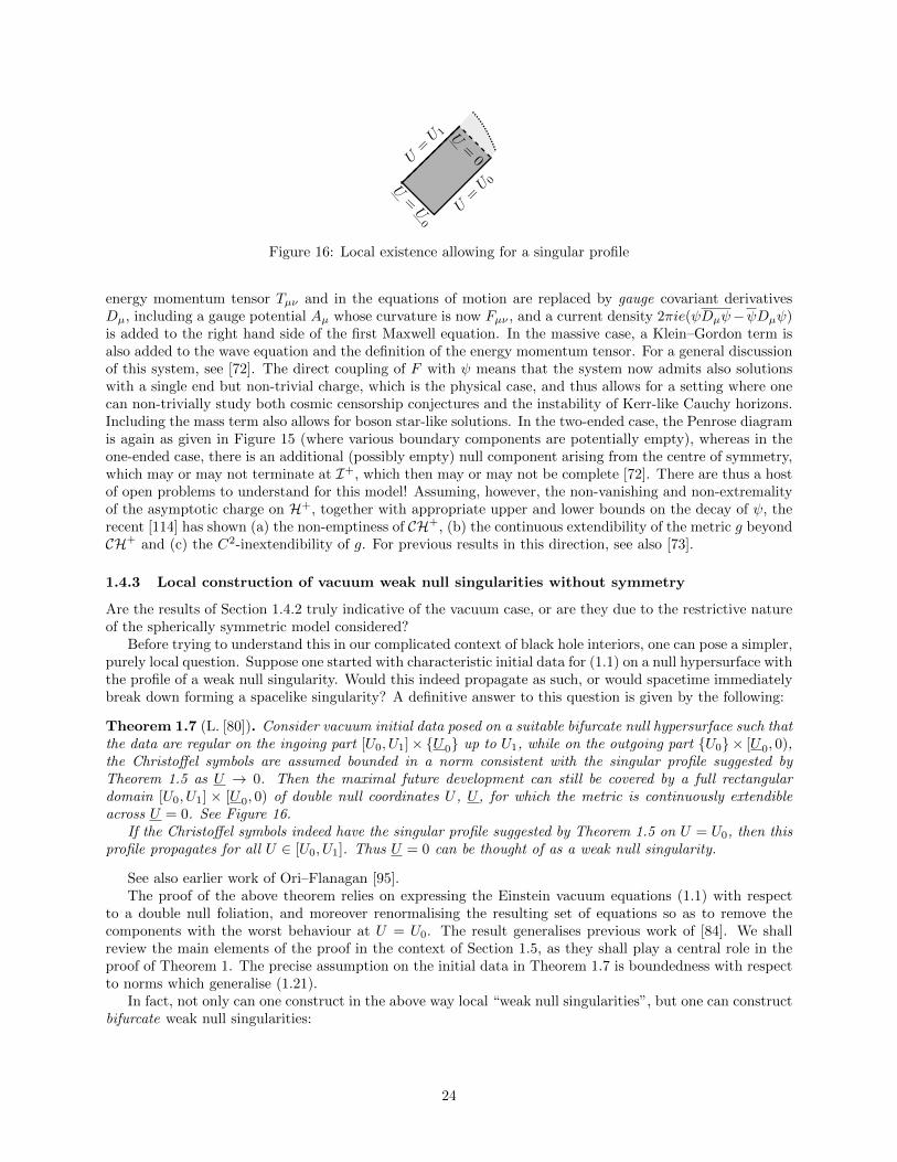
U=U 0

U=

0U=U 1

U=U0

Figure 16: Local existence allowing for a singular profile

energy momentum tensor Tµν and in the equations of motion are replaced by gauge covariant derivativesDµ, including a gauge potential Aµ whose curvature is now Fµν , and a current density 2πie(ψDµψ−ψDµψ)is added to the right hand side of the first Maxwell equation. In the massive case, a Klein–Gordon term isalso added to the wave equation and the definition of the energy momentum tensor. For a general discussionof this system, see [72]. The direct coupling of F with ψ means that the system now admits also solutionswith a single end but non-trivial charge, which is the physical case, and thus allows for a setting where onecan non-trivially study both cosmic censorship conjectures and the instability of Kerr-like Cauchy horizons.Including the mass term also allows for boson star-like solutions. In the two-ended case, the Penrose diagramis again as given in Figure 15 (where various boundary components are potentially empty), whereas in theone-ended case, there is an additional (possibly empty) null component arising from the centre of symmetry,which may or may not terminate at I+, which then may or may not be complete [72]. There are thus a hostof open problems to understand for this model! Assuming, however, the non-vanishing and non-extremalityof the asymptotic charge on H+, together with appropriate upper and lower bounds on the decay of ψ, therecent [114] has shown (a) the non-emptiness of CH+, (b) the continuous extendibility of the metric g beyondCH+ and (c) the C2-inextendibility of g. For previous results in this direction, see also [73].

1.4.3 Local construction of vacuum weak null singularities without symmetry

Are the results of Section 1.4.2 truly indicative of the vacuum case, or are they due to the restrictive natureof the spherically symmetric model considered?

Before trying to understand this in our complicated context of black hole interiors, one can pose a simpler,purely local question. Suppose one started with characteristic initial data for (1.1) on a null hypersurface withthe profile of a weak null singularity. Would this indeed propagate as such, or would spacetime immediatelybreak down forming a spacelike singularity? A definitive answer to this question is given by the following:

Theorem 1.7 (L. [80]). Consider vacuum initial data posed on a suitable bifurcate null hypersurface such thatthe data are regular on the ingoing part [U0, U1]×U0 up to U1, while on the outgoing part U0× [U0, 0),the Christoffel symbols are assumed bounded in a norm consistent with the singular profile suggested byTheorem 1.5 as U → 0. Then the maximal future development can still be covered by a full rectangulardomain [U0, U1] × [U0, 0) of double null coordinates U , U , for which the metric is continuously extendibleacross U = 0. See Figure 16.

If the Christoffel symbols indeed have the singular profile suggested by Theorem 1.5 on U = U0, then thisprofile propagates for all U ∈ [U0, U1]. Thus U = 0 can be thought of as a weak null singularity.

See also earlier work of Ori–Flanagan [95].The proof of the above theorem relies on expressing the Einstein vacuum equations (1.1) with respect

to a double null foliation, and moreover renormalising the resulting set of equations so as to remove thecomponents with the worst behaviour at U = U0. The result generalises previous work of [84]. We shallreview the main elements of the proof in the context of Section 1.5, as they shall play a central role in theproof of Theorem 1. The precise assumption on the initial data in Theorem 1.7 is boundedness with respectto norms which generalise (1.21).

In fact, not only can one construct in the above way local “weak null singularities”, but one can constructbifurcate weak null singularities:

24

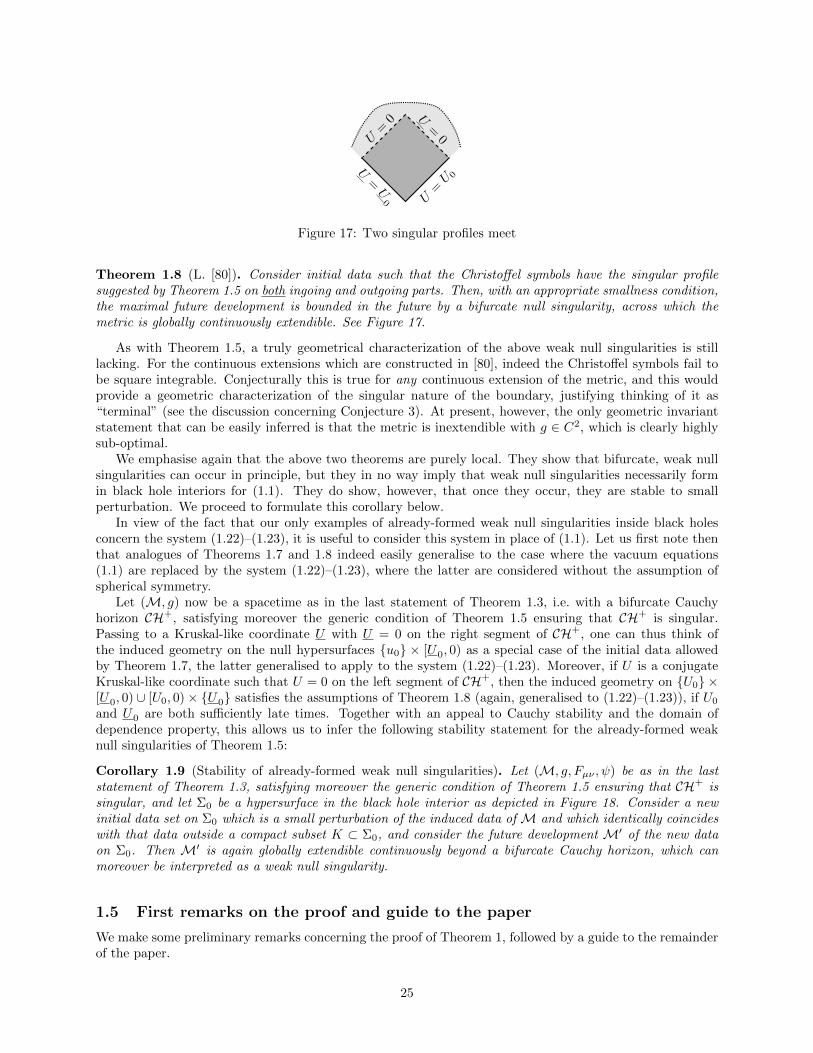
U=

0

U=U 0

U=U0

U=

0

Figure 17: Two singular profiles meet

Theorem 1.8 (L. [80]). Consider initial data such that the Christoffel symbols have the singular profilesuggested by Theorem 1.5 on both ingoing and outgoing parts. Then, with an appropriate smallness condition,the maximal future development is bounded in the future by a bifurcate null singularity, across which themetric is globally continuously extendible. See Figure 17.

As with Theorem 1.5, a truly geometrical characterization of the above weak null singularities is stilllacking. For the continuous extensions which are constructed in [80], indeed the Christoffel symbols fail tobe square integrable. Conjecturally this is true for any continuous extension of the metric, and this wouldprovide a geometric characterization of the singular nature of the boundary, justifying thinking of it as“terminal” (see the discussion concerning Conjecture 3). At present, however, the only geometric invariantstatement that can be easily inferred is that the metric is inextendible with g ∈ C2, which is clearly highlysub-optimal.

We emphasise again that the above two theorems are purely local. They show that bifurcate, weak nullsingularities can occur in principle, but they in no way imply that weak null singularities necessarily formin black hole interiors for (1.1). They do show, however, that once they occur, they are stable to smallperturbation. We proceed to formulate this corollary below.

In view of the fact that our only examples of already-formed weak null singularities inside black holesconcern the system (1.22)–(1.23), it is useful to consider this system in place of (1.1). Let us first note thenthat analogues of Theorems 1.7 and 1.8 indeed easily generalise to the case where the vacuum equations(1.1) are replaced by the system (1.22)–(1.23), where the latter are considered without the assumption ofspherical symmetry.

Let (M, g) now be a spacetime as in the last statement of Theorem 1.3, i.e. with a bifurcate Cauchyhorizon CH+, satisfying moreover the generic condition of Theorem 1.5 ensuring that CH+ is singular.Passing to a Kruskal-like coordinate U with U = 0 on the right segment of CH+, one can thus think ofthe induced geometry on the null hypersurfaces u0 × [U0, 0) as a special case of the initial data allowedby Theorem 1.7, the latter generalised to apply to the system (1.22)–(1.23). Moreover, if U is a conjugateKruskal-like coordinate such that U = 0 on the left segment of CH+, then the induced geometry on U0 ×[U0, 0) ∪ [U0, 0)× U0 satisfies the assumptions of Theorem 1.8 (again, generalised to (1.22)–(1.23)), if U0

and U0 are both sufficiently late times. Together with an appeal to Cauchy stability and the domain ofdependence property, this allows us to infer the following stability statement for the already-formed weaknull singularities of Theorem 1.5:

Corollary 1.9 (Stability of already-formed weak null singularities). Let (M, g, Fµν , ψ) be as in the laststatement of Theorem 1.3, satisfying moreover the generic condition of Theorem 1.5 ensuring that CH+ issingular, and let Σ0 be a hypersurface in the black hole interior as depicted in Figure 18. Consider a newinitial data set on Σ0 which is a small perturbation of the induced data of M and which identically coincideswith that data outside a compact subset K ⊂ Σ0, and consider the future development M′ of the new dataon Σ0. Then M′ is again globally extendible continuously beyond a bifurcate Cauchy horizon, which canmoreover be interpreted as a weak null singularity.

1.5 First remarks on the proof and guide to the paper

We make some preliminary remarks concerning the proof of Theorem 1, followed by a guide to the remainderof the paper.

25

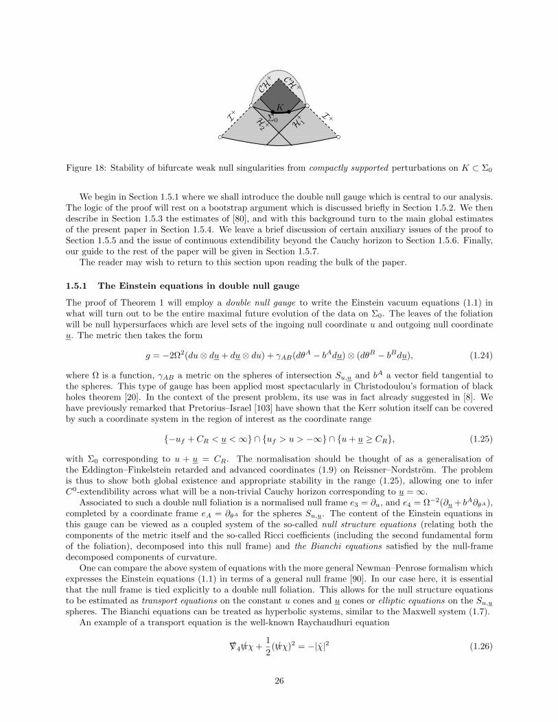
Σ0

K

I+ I +H +

2 H+

1

CH+ CH +

Figure 18: Stability of bifurcate weak null singularities from compactly supported perturbations on K ⊂ Σ0

We begin in Section 1.5.1 where we shall introduce the double null gauge which is central to our analysis.The logic of the proof will rest on a bootstrap argument which is discussed briefly in Section 1.5.2. We thendescribe in Section 1.5.3 the estimates of [80], and with this background turn to the main global estimatesof the present paper in Section 1.5.4. We leave a brief discussion of certain auxiliary issues of the proof toSection 1.5.5 and the issue of continuous extendibility beyond the Cauchy horizon to Section 1.5.6. Finally,our guide to the rest of the paper will be given in Section 1.5.7.

The reader may wish to return to this section upon reading the bulk of the paper.

1.5.1 The Einstein equations in double null gauge

The proof of Theorem 1 will employ a double null gauge to write the Einstein vacuum equations (1.1) inwhat will turn out to be the entire maximal future evolution of the data on Σ0. The leaves of the foliationwill be null hypersurfaces which are level sets of the ingoing null coordinate u and outgoing null coordinateu. The metric then takes the form

g = −2Ω2(du⊗ du+ du⊗ du) + γAB(dθA − bAdu)⊗ (dθB − bBdu), (1.24)

where Ω is a function, γAB a metric on the spheres of intersection Su,u and bA a vector field tangential tothe spheres. This type of gauge has been applied most spectacularly in Christodoulou’s formation of blackholes theorem [20]. In the context of the present problem, its use was in fact already suggested in [8]. Wehave previously remarked that Pretorius–Israel [103] have shown that the Kerr solution itself can be coveredby such a coordinate system in the region of interest as the coordinate range

−uf + CR < u <∞ ∩ uf > u > −∞ ∩ u+ u ≥ CR, (1.25)

with Σ0 corresponding to u + u = CR. The normalisation should be thought of as a generalisation ofthe Eddington–Finkelstein retarded and advanced coordinates (1.9) on Reissner–Nordstrom. The problemis thus to show both global existence and appropriate stability in the range (1.25), allowing one to inferC0-extendibility across what will be a non-trivial Cauchy horizon corresponding to u =∞.

Associated to such a double null foliation is a normalised null frame e3 = ∂u, and e4 = Ω−2(∂u + bA∂θA),completed by a coordinate frame eA = ∂θA for the spheres Su,u. The content of the Einstein equations inthis gauge can be viewed as a coupled system of the so-called null structure equations (relating both thecomponents of the metric itself and the so-called Ricci coefficients (including the second fundamental formof the foliation), decomposed into this null frame) and the Bianchi equations satisfied by the null-framedecomposed components of curvature.

One can compare the above system of equations with the more general Newman–Penrose formalism whichexpresses the Einstein equations (1.1) in terms of a general null frame [90]. In our case here, it is essentialthat the null frame is tied explicitly to a double null foliation. This allows for the null structure equationsto be estimated as transport equations on the constant u cones and u cones or elliptic equations on the Su,uspheres. The Bianchi equations can be treated as hyperbolic systems, similar to the Maxwell system (1.7).

An example of a transport equation is the well-known Raychaudhuri equation

/∇4 /trχ+1

2(/trχ)2 = −|χ|2 (1.26)

26

relating two Ricci coefficients, the outgoing expansion /trχ and the shear χ, whereas an elliptic equation isgiven by

/div χ =1

2/∇/trχ− η · (χ− /trχγ)− β, (1.27)

relating the shear χ with the curvature component βA = 12R(eA, e4, e3, e4). The one-form ηA appearing

above is an additional Ricci coefficient. Here and in the formulas that follow, /∇3 and /∇4 are covariantdifferential operator in the direction of e3 and e4, respectively while /∇, /div denote differential operatorsassociated to the Su,u-spheres. Note that the above Ricci coefficients both also satisfy transport equationsin the e3 direction:

/∇3 /trχ+1

2/trχ /trχ = 2ω /trχ+ 2ρ− χ · χ+ 2 /div η + 2|η|2, (1.28)

/∇3χ+1

2/trχχ = /∇⊗η + 2ωχ− 1

2/trχχ+ η⊗η. (1.29)

In the formula above, we see the Ricci coefficient ω, defined by

ω = − /∇3(log Ω) (1.30)

as well as various conjugate quantities to the ones we have defined, where the roles of e3 and e4 are inter-changed with various sign conventions.

The curvature component β together with the couple (ρ = 14R(e4, e3, e4, e3), σ = 1

4∗R(e4, e3, e4, e3)) can

be thought of as a “Bianchi pair” related by the equations

/∇3β + /trχβ = /∇ρ+∗ /∇σ + 2ωβ + 2χ · β + 3(ηρ+∗ ησ), (1.31)

/∇4σ+3

2/trχσ = − /div

∗β+

1

2χ∧α− ζ ∧β− 2η∧β, /∇4ρ+

3

2/trχρ = /div β− 1

2χ ·α+ ζ ·β+ 2η ·β. (1.32)

Here ∗ denotes Hodge dual. In estimating (1.31)–(1.32) as a hyperbolic system one exploits the fact thatthe angular operators ( /∇,∗ /∇) and /div can be viewed as L2 adjoints on the spheres Su,u.

As first understood in the context of the monumental proof of the stability of Minkowski space byChristodoulou–Klainerman [21], use of (1.26) and (1.27) together (as well as related pairs of transport andelliptic equations involving /trχ and the quantities µ, µ and ω/ to be discussed later) allows one to eventuallyestimate all Ricci coefficients at one level of differentiability greater than curvature. Briefly, the point isthat neither curvature nor first derivatives of Ricci coefficients appear on the right hand side of (1.26) andthus, integration of (1.26) does not lose a derivative, in contrast to the generic transport equation, like(1.28)–(1.29), for which one sees /div η and /∇⊗η. On the other hand, the elliptic equation (1.27) gains aderivative with respect its right hand side, where the curvature term β is present.

1.5.2 The bootstrap argument and the logic of the proof

As with many non-linear analyses for the Einstein vacuum equations (1.1), the proof of Theorem 1 willproceed via the method of continuity (or “bootstrap”). One considers the set I ⊂ (−uf + CR,∞) ofuc ∈ (−uf + CR,∞) such that there exists a solution of the form (1.24) on

−uf + CR < u < uc ∩ uf > u > −uc + CR ∩ u+ u ≥ CR, (1.33)

satisfying a number of estimates, known in this context as “bootstrap assumptions” (see already (1.42)below). This region is depicted as the darker shaded region in Figure 19.

This set I is non-empty by a suitable local existence result and it will be manifestly closed by the natureof the inequalities. Finally, we shall show that the set is open by “improving the bootstrap assumptions”,i.e. by (a) proving estimates on all quantities, including stronger estimates than the assumed bootstrapassumptions, and then (b) applying local existence again to obtain that the stronger estimates hold in aslightly larger region. It will follow that I = (−uf +CR,∞) and thus the solution exists on the entire domain(1.25).

In Section 1.5.4 below, we will focus entirely on (a), i.e. on proving estimates on the solution in a region(1.33) on which the solution is already known to exist. We will return to discuss the completion of thebootstrap argument in Section 1.5.5.

27

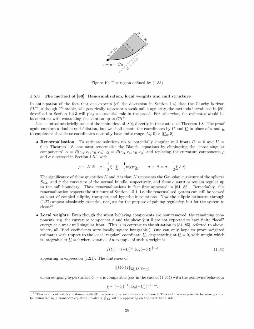
u=∞

u+ u = CRu

=−∞

u=u f

u=uc

Figure 19: The region defined by (1.33)

1.5.3 The method of [80]: Renormalisation, local weights and null structure

In anticipation of the fact that one expects (cf. the discussion in Section 1.4) that the Cauchy horizonCH+, although C0 stable, will generically represent a weak null singularity, the methods introduced in [80]described in Section 1.4.3 will play an essential role in the proof. For otherwise, the estimates would beinconsistent with controlling the solution up to CH+.

Let us introduce briefly some of the main ideas of [80], directly in the context of Theorem 1.8. The proofagain employs a double null foliation, but we shall denote the coordinates by U and U in place of u and uto emphasise that these coordinates naturally have finite range [U0, 0)× [U0, 0).

• Renormalisation. To estimate solutions up to potentially singular null fronts U = 0 and U =0 in Theorem 1.8, one must renormalise the Bianchi equations by eliminating the “most singularcomponents” α = R(eA, e4, eB , e4), α = R(eA, e3, eB , e3) and replacing the curvature components ρand σ discussed in Section 1.5.1 with

ρ K.= −ρ+

1

2χ · χ− 1

4/trχ/trχ, σ σ = σ +

1

2χ ∧ χ.

The significance of these quantities K and σ is that K represents the Gaussian curvature of the spheresSU,U and σ the curvature of the normal bundle, respectively, and these quantities remain regular upto the null boundary. These renormalisations in fact first appeared in [84, 85]. Remarkably, thisrenormalisation respects the structure of Section 1.5.1, i.e. the renormalised system can still be viewedas a set of coupled elliptic, transport and hyperbolic equations. Now the elliptic estimates through(1.27) appear absolutely essential, not just for the purpose of gaining regularity, but for the system toclose.26

• Local weights. Even though the worst behaving components are now removed, the remaining com-ponents, e.g. the curvature component β and the shear χ still are not expected to have finite “local”energy at a weak null singular front. (This is in contrast to the situation in [84, 85], referred to above,where, all Ricci coefficients were locally square integrable.) One can only hope to prove weightedestimates with respect to the local “regular” coordinate U , degenerating at U = 0, with weight whichis integrable at U = 0 when squared. An example of such a weight is

f(U) = (−U)12 | log(−U)| 12 +δ (1.34)

appearing in expression (1.21). The finiteness of

‖f(U)χ‖L2UL

2(SU,U )

on an outgoing hypersurface U = c is compatible (say in the case of (1.34)) with the pointwise behaviour

χ ∼ (−U)−1| log(−U)|−1−2δ.

26This is in contrast, for instance, with [31], where elliptic estimates are not used. This in turn was possible because χ couldbe estimated by a transport equation involving /∇4χ with α appearing on the right hand side.

28

Note that this is in turn compatible with the finiteness of the L1 norm

‖χ‖L1UL

2(SU,U ),

which is to be expected if the metric is to be continuously extendible beyond U = 0.

For a linear equation like (1.4), such weighted estimates are readily seen to locally propagate. For thenon-linear Einstein equations (1.1), however, the question of the local propagation of such weightedestimates becomes highly non-trivial, dependent on the precise null structure in the nonlinearities.

• Schematic notation and null structure. In order to describe the above structure, it is useful tofirst introduce a schematic notation.27 One can group (a subset of) the Ricci coefficients into familiesas follows:

ψ ∈ η, η, ψH ∈ /trχ, χ, ψH ∈ /trχ, χ

according to their expected singular behaviour. All terms ψH have expected behaviour similar toχ (and β) and thus can be estimated either in L1

UL2(S) on outgoing hypersurfaces U = c, or with

the weight (1.34) in L2UL

2(S). Analogous statements hold for ψH with ingoing hypersurfaces U = creplacing outgoing ones. The terms ψ, on the other hand, can be estimated without degeneration.Energy identities for β lead in particular to having to estimate spacetime integrals of the form

‖f2(U)(βψHβ + βψHβ + βψK)‖L1UL

1UL

1(S) (1.35)

All the terms appearing above can be seen to be admissible from the point of view of integrability. Incontrast, terms like βψHβ or βψHβ would not have been controllable. It is thus precisely the absenceof such terms which captures the “null structure” essential for this argument.

Of course, the story is more complicated, in that the equations need to be sufficiently commuted sothat indeed trilinear terms can be controlled by top order L2 estimates and Sobolev inequalities. We deferdiscussion of these issues to the setting of our actual problem in Section 1.5.4 below.

1.5.4 The main estimates

Already in the context of the linear wave equation (1.4) discussed in Section 1.4.1, it is clear that weightedestimates with respect to the (infinite-range) coordinates u and u are necessary in view of the global aspectsof the problem special to the black hole interior.

The remarkable fact, central to the present work, is that these two systems of weights, thoseintroduced in the study of the wave equation as discussed in Section 1.4.1 and those introducedin [80] as discussed in Section 1.4.3, are in fact compatible, and the null condition is reflectedin both.

Indeed, we have already seen that the polynomially growing weight in u, coupled with the degeneratecoordinate derivative ∂u and degenerate one-form du, when looked at for fixed u, behaves precisely like(1.21).

We outline below the main ideas in adapting the global weighted estimates of (1.4), combined with therenormalisation of Section 1.5.3, to the global analysis of the Einstein vacuum equations (1.1) in the blackhole interior.

• Differences, angular commutation and reduced schematic notation. First of all, it is nowdifferences which must be estimated, i.e. one must subtract from each quantity, e.g. the outgoingexpansion /trχ or the curvature component β, its Kerr value, considering

/trχ.= /trχ− (/trχ)K, β

.= β − βK. (1.36)

We will extend the schematic notation of Section 1.5.3 to differences by defining

ψ ∈ η, η , ψH ∈ /trχ, ˜χ , ψH ∈ /trχ, ˜χ27The notation and conventions of [80] are slightly different. Here we follow notation to be used in the present paper.

29

and defining also a schematic notation for difference quantities at the level of the metric itself:

g ∈ γAB − (γAB)K, . . . , log Ω− log ΩK.

We note already that the metric component b and the Ricci coefficient difference ω defined from (1.30)do not have a schematic representation and must always be dealt with explicitly. Moreover, for ourestimates to close, we will need to control quantities in a higher Lp norm via Sobolev inequalities (seealso Section 1.5.5 below!), so we will have to commute (in the angular directions /∇) the null structureequations for the Ricci coefficients up to three times, and the Bianchi equations up to two times, i.e. we

shall consider quantities /∇3ψ,. . . /∇2

β,. . . .28 After commuting the equations, we shall moreover adoptthe convention that lower order terms which can be controlled in L∞ will not be written explicitly. Thesystem for differences will retain the structural properties of the renormalised system, but gives riseto additional “inhomogeneous” terms. We shall call this system the “reduced schematic equations”.They are derived in Section 7.

For instance, the equation for /∇3/trχ arising from taking differences and commuting (1.26) can be

written in reduced schematic form as

/∇4 /∇3/trχ =RS

∑i1+i2+i3≤3

(1 + /∇i1 g + /∇mini1,2ψ)(1 + /∇i2 ψH)( /∇i3(ψH , g) + Ω−2K /∇i3 b), (1.37)

where =RS denotes that the relation holds in the sense of our conventions described above. As we

shall see, the quantity /trχ has a special role in the context of not losing differentiability for the secondfundamental form (cf. the discussion at the end of Section 1.5.1). We remark already that the equation

(1.37) does not contain top-order terms (e.g. terms like /∇3ψ or /∇2

β on its right hand side).

• Global weights in ΩK, $N , u and u. In contrast to the case of the linear scalar wave equation(1.4), there is no longer a standard Lagrangian structure naturally giving rise to weighted estimatesvia vector fields such as (1.13), so the weights must be put in by hand in a more ad hoc fashion in

the context of direct integration by parts. For instance, the curvature difference quantity β of (1.36)is estimated in the weighted norm

‖u 12 +δ$NΩ2

Kβ‖L∞u L2uL

2(Su,v). (1.38)

Comparing the above expression to the first expression in (1.14) which arose as a flux of the vector field(1.13), we note that Ω2

Ke4 is in some sense equivalent to ∂u, and we see the quantity rN is replaced by$N , appropriate for Kerr, as discussed in Section 1.4.1.

• The controlling energies N . As remarked already, the top-order estimates will be at the level of

two angular commutations of curvature, e.g. /∇2β. In view of the elliptic estimates mentioned already

in Section 1.5.1 (see also below), we will be able to estimate all terms /∇3ψ, /∇3

ψH , /∇3ψH , from top-

order curvature terms, and conversely. This motivates defining a certain master energy, defined withreference only to the metric and Ricci coefficients, which will finally be shown to control the entiresystem.

The master energy is in fact best separated into three parts, some of whose terms are displayed below:

Nhyp = ‖u 12 +δ$NΩ2

K /∇3ψH‖2L∞u L2

uL2(S) + ‖|u| 12 +δ$N /∇3

ψH‖2L∞u L2uL

2(S) + · · · (1.39)

Nint = ‖u 12 +δ$NΩ3

K /∇3ψH‖2L2

uL2uL

2(S) + ‖|u|12 +δ

$NΩK /∇3ψH‖2L2

uL2uL

2(S)

+‖u 12 +δ$NΩK /∇

3ψ‖2L2

uL2uL

2(S) · · · (1.40)

Nsph = ‖ /∇3g‖2L∞u L∞u L2(S) + · · ·+ ‖ψH‖2L1

uL∞u L

2(S) + · · · . (1.41)

28Compare with the role of commutation in obtaining the L∞ estimate (1.20). Note that in view of the lack of exactly

commuting operators Wi, it is more natural to commute tensorially here, just as in [84, 85, 31]. Note that /∇iψ is a higher rankSu,u-tensor than ψ.

30

We note that the energy Nhyp of (1.39), which consists of null hypersurface integrals, controls in

particular all the top order flux terms of curvature, for instance (1.38) where β is replaced by /∇2β.

See already Section 4.6.5 for the complete definitions of these energies.

The energy Nint of (1.40) consists of spacetime integrals. The integrals in the first line of (1.40) aretypically generated by good-sign bulk terms in energy identities which arise from the insertion of agood weight like $N above, cf. (1.16) that arose in estimates for the wave equation (1.4). The termdisplayed in the second line of (1.40) is analogous to (1.17). As with (1.4), the latter term miraculouslynaturally appears in various estimates with a good sign. Note, however, the different ΩK weightscomparing (1.39) with (1.40), signifying that (1.40) is more degenerate and thus gives less control.

Finally, the energy Nsph of (1.41) gives higher Lp control on lower order terms. We remark alreadythat on lower order terms, the order of L∞ norm is inside, providing a stronger estimate than otherwise.See for instance the second term of (1.41). This will be crucial, because for the top order terms likethe first two terms of (1.39), the L∞ norm will have to be taken outside.

We note that the bootstrap assumption (cf. Section 1.5.2) can in fact be expressed entirely in terms of(1.41) as

Nsph ≤ ε. (1.42)

Given (1.42), our estimates for the null structure equations and the Bianchi identities (see below!) willallow us to estimate

Nhyp . ε2, Nint . ε2 (1.43)

provided that an initial data quantity D satisfies

D ≤ ε2, (1.44)

for ε sufficiently small. Finally, this will allow us to infer (using the null structure equations togetherwith 1-dimensional Sobolev inequalities) that

Nsph . ε2, (1.45)

which, for ε sufficiently small, improves (1.42). This will then complete part (a) of the bootstrapargument as outlined in Section 1.5.2.

We thus turn in the remainder of this section to a discussion of how to obtain (1.43).

• Transport estimates for Ricci coefficients and wave-type estimates for curvature. In general,the Ricci coefficients will be estimated via integrating transport equations while the curvature will beestimated from the Bianchi identities. Since the Bianchi identities encode the hyperbolic aspect ofthe Einstein vacuum equations (1.1) expressed in a double null gauge, they are in some sense mostanalogous to the linear wave equation (1.4), their tensorial structure not withstanding. In particular,energy estimates with weights related to those described in Section 1.4.1 (see already Section 10)would indeed allow one to obtain (1.43) for some of the top order terms displayed in (1.39) and (1.40),provided that certain “error terms” can be controlled, which can be classified into various types E1,E2, T1, F2. (These are defined in Section 8.)

The analogous estimates for Ricci coefficients are simpler (and precede the treatment of curvature in thepaper; see already Section 9), following by weighted estimates applied directly to transport equations.This again allows for control of all of the lower order estimates for Ricci coefficients displayed in (1.39)and (1.40), conditional on being able to recover estimates for error terms. Before turning to the toporder estimates for the remaining Ricci coefficients let us discuss how some of these error terms areestimated.

• Estimating error terms. Let us examine briefly two types of error terms that arise in the process

of estimating the second term of (1.38) at highest order (where β is replaced by /∇2β), via the Bianchi

identities. See already Section 12.

31

We have already seen in Section 1.5.3 one type of error term which arises, namely, those arising fromthe nonlinearities. An example of such a term is:

‖u1+2δ$2NΩ4K /∇

3ψH /∇

3ψH ψH‖L1

uL1uL

1(S). (1.46)

Note that this is analogous to the first term of (1.35). In the notation of Section 8, this term arisesfrom one of the error terms contained in T2. It can be easily bounded by the first term of (1.39) andthe second term of (1.41), noting the importance of the order of the L1L∞ norm in (1.41). Again,we see here a manifestation of the “null condition”. (See already the proof of Proposition 12.5 ofSection 12.3.)

Another type of error term which arises are linear inhomogeneous terms that are generated from theprocess of taking differences. An example of such a term that must be estimated is

‖u 12 +δ$NΩK /∇

3ψH‖L2

uL2uL

2(S). (1.47)

In the notation of Section 8, this term arises from one of the error terms contained in E1. (Note thatthis term is not directly controlled by the second term of Nint in (1.40) since |u| . u.) For (1.47), wemust divide the region of integration into −u > 1

2u and −u < 12u. In the first region, we may replace

u by |u| and estimate this term by the second term of (1.40). In the second region, we use the bound

supSu,u

|ΩK|(u, u) . e−12κ−u, sup

Su,u

u12 +δ|ΩK|(u, u) . e−

14κ−u

to bound (1.47) restricted to this region by

‖|u| 12 +δ$N /∇3ψH‖L∞u L2

uL2(S)‖e−

14κ−u‖L∞u L2

u,

which can now be bound by (1.39). Here κ− = r+−r−2(r2−+a2)

denotes the surface gravity of the Kerr Cauchy

horizon. (See already the proof of Proposition 12.2 of Section 12.2.)

• Top order estimates for Ricci coefficients. To obtain (1.43) for the remaining top-order quantities,i.e. those that cannot be directly related to curvature, is tricky because one must at the same time usethe structure described at the end of Section 1.5.1 and still be be compatible with the global weights.See already Section 11.

For instance, for top order estimates we must estimate the quantity /trχ via the commuted Raychaudhuriequation (1.37).

To handle the conjugate quantity /trχ via its analogous Raychaudhuri equation, we re-express thatequation in terms of the geodesic vector field to avoid the worst coupling with ω. Recall that thislatter Ricci coefficient does not have a schematic representation, and has anomalous decay properties.

(The renormalised form of the transport equation satisfied by /trχ is given in Proposition 7.19 and isused in the proof of Proposition 11.10.)

The importance of the “null condition” for either long term existence or local regularity issues has beenmade clear many times in previous work on the Einstein equations (1.1). The former role is most famouslyrepresented by the monumental proof of the stability of Minkowski space [21], while the latter role can beseen in the works [84, 80], discussed above, as well as the proof of the bounded L2 curvature conjecture [71].In this context, it is interesting to remark how in the present work, our weights in u and u capture bothroles of null structure, seamlessly transitioning as u → ∞ from their role in proving sufficiently long-timeexistence to their role in ensuring the propagation of low regularity.

1.5.5 Auxiliary issues

Let us briefly comment on certain auxiliary issues in the proof which we have not emphasised so far.

32

• Initial data and local existence. An initial data set for (1.1) constitutes a triple (Σ0, g, k) satisfyingthe Einstein constraint equations (see already (4.1)). The first version of our theorem (stated asTheorem 4.2) will give a smallness condition expressed solely in terms of the geometric initial data

g and k. Applying well posedness in the smooth category [15], together with ode arguments, wewill be able to construct locally a double null gauge (1.24) which will be the non-emptiness step ofthe bootstrap argument. We can also globally re-express the initial data in terms of the quantitiesassociated to (1.24). This will allow us to give a more precise version of the theorem (stated asTheorem 4.27), identifying the smallness condition (1.44), in terms directly related to the quantities(1.39), (1.41) appearing in estimates.

• Sobolev and ellipticity constants. The estimates described in Section 1.5.4 require being able toapply the Sobolev inequality to handle lower order terms, and exploiting ellipticity of equations like(1.27). This in turn requires quantitative control of various Sobolev constants with respect to theinduced geometry of the spheres Su,u, and some a priori input on the behaviour of the metric will benecessary. The bootstrap assumption (1.42) will suffice for this, and thus bounding these constantsis in fact the first task of the proof, handled already in Section 5. Note that the conventions relatedto the reduced schematic equations hide many terms estimated by Sobolev, for instance, already inwriting (1.37).

• Propagation of higher regularity. As in Christodoulou’s formation of black holes work [20], forshowing the extendibility of our solution (in the context of step (b) of the bootstrap argument describedin Section 1.5.2) we will appeal to a local existence result in the C∞ category, just as we have doneabove to show that the evolution is non-empty.29 On the other hand, the main estimates described inSection 1.5.4 close at the finite regularity defined by the quantities (1.39)–(1.41). Thus, to completestep (b) of Section 1.5.2, we need to show first the propagation of higher regularity. These estimates aretypically very straightforward because the equations are linear in the highest order quantities, and oneonly requires the finiteness for given u, not uniform control as u → ∞. Nonetheless, in our problem,special care has to be made, however, since, by having renormalised our system as in Section 1.5.3, theenergies (1.39)–(1.41) no longer control all relevant quantities. This will be the subject of Section 14.

1.5.6 The continuity of the extension

Having shown global existence up to the boundary u = ∞, the last step in the proof of Theorem 1 is toshow that the metric is indeed continuously extendible beyond. This will require certain additional estimates

on the quantity /∇4 log Ω (see already Proposition 16.2). In addition to defining—in complete analogy withwhat was already done in the proof of Theorem 1.3 concerning the spherically symmetric toy model ofSection 1.4.2—a rescaled coordinate U = uCH+ , proving continuity now also requires redefining the angularcoordinates (θACH+) which effectively serves to renormalise the metric coefficient b. We will show in additionthat the spacetime remains close to Kerr in the C0 norm. This will be the subject of Section 16.

1.5.7 Outline of the paper

We end this guide to the paper with a brief section-by-section account of its contents (referring back to ourdiscussion above when relevant).

We begin in Section 2 with a general discussion of the double null gauge (1.24) defined on a suitabledomain U , in particular, putting the Kerr metric in this framework.

We then present in Section 3 the Einstein vacuum equations (1.1) written in this gauge, moving immedi-ately to the renormalised form (described above in Section 1.5.3), and introducing the schematic notations ψ,ψH and ψH . This will allow us in Section 4 to set up the initial value problem with initial data (Σ0, g, K),giving the two progressively more detailed (cf. the discussion above in Section 1.5.5) statements of Theo-rem 1, given as Theorem 4.2 and Theorem 4.24, as well as the statement of the main estimates in thebootstrap region Uuf , Theorem 4.27 (cf. the discussion in Section 1.5.2).

29We shall need both local existence for the standard Cauchy problem, for which we quote [15], but also for a characteristicinitial value problem. One could quote [104], but it will in fact be more convenient to appeal to a local existence for theequations expressed already in the double null gauge, as this ensures that one can obtain a whole neighbourhood of an initialingoing hypersurface. See already Section 15.

33

Sections 5–13 will concern the proof of Theorem 4.27. We shall use the bootstrap assumption to obtainin Section 5 preliminary bounds in Uuf on Sobolev constants and ellipticity estimates which will be useful

throughout (cf. Section 1.5.5). This will allow us to derive a general estimate for quantities satisfyingcovariant transport equations in Section 6. We then derive in Section 7 the “reduced schematic equations”for differences, which incorporate L∞ bounds derived by Sobolev that hold in Uuf . Section 8 will definethe error expressions E1, E2, T1, T2 and state Proposition 8.1, which corresponds to the main estimate forthe quantities Nint and Nhyp in terms of these error expressions (cf. the discussion above in Section 1.5.4).The proof of Proposition 8.1 will then occupy the next three sections: Section 9 will bound the Riccicoefficients via transport estimates for the null structure equations, Section 10 will bound the curvature viaenergy estimates for the Bianchi equations and Section 11 will bound the remaining top order estimates forRicci coefficients using elliptic estimates. Finally, the error terms on the right hand side of the estimate ofProposition 8.1 will be themselves estimated in Section 12, thus completing the proof of the boundedness ofNint and Nhyp in Uuf , stated as Proposition 12.1 (cf. (1.43)). The bootstrap assumptions will be recovered

in Section 13 (cf. (1.45)), completing the proof of Theorem 4.27.With Theorem 4.27, proven, we turn in Section 14 to the propagation of higher regularity discussed

above in Section 1.5.5, which, together with an application of local existence, will allow us in Section 15 toobtain the global existence part of Theorem 4.24 from Theorem 4.27, stated as Theorem 15.6. This yieldsthe existence of a solution on U∞.

It will remain only to identify the solution (U∞, g) as the maximal Cauchy development of data, andshow the continuous extendibility of the metric beyond a non-trivial Cauchy horizon (Theorem 16.14);this will be accomplished in Section 16, completing the proof of Theorem 4.24.

Although in this paper we do not show that the Cauchy horizon is in any sense generically singular, weend our paper in Section 17 with a discussion of the compatibility of our estimates with the Cauchy horizonbeing a weak null singularity in the sense of [80]. This is given as Theorem 17.1.

Several computations relating to the Kerr metric in double null gauge are relegated to Appendix A.

1.6 Addendum: the case Λ 6= 0

As is well known, Einstein entertained early on a certain modification [43] of his equations (1.1) by addinga non-vanishing “cosmological” constant Λ:

Ricµν −1

2gµνR+ Λgµν = 8πTµν . (1.48)

This constant Λ is known observationally to be very small, effectively zero for the scale of astrophysicalblack holes which motivate the considerations of this paper. As of the present writing, however, the case of asmall Λ > 0 is favoured on so-called “cosmological” scales where the universe is thought to be approximatelyisotropic and homogeneous, and can be described with an energy momentum tensor corresponding to dust.In contrast, the case Λ < 0 can be related to various speculations in high energy physics, and has receivedmuch recent interest in that context [53].

In the vacuum, equation (1.48) reduces to

Ricµν = Λgµν . (1.49)

The “trivial” solution of (1.49) with Λ > 0 was first studied in [39] and is known as de Sitter space. Theanalogous solution for Λ < 0 is traditionally known as anti-de Sitter space [58]. There is a generalisationof the Kerr family to (1.49), known as Kerr–de Sitter in the positive case and Kerr–anti de Sitter in thenegative case which contain analogues of “black holes”. These solutions are unfortunately not contained inthe standard elementary textbooks, but one can find a detailed discussion of their geometry in [14].

The cosmological case Λ > 0. In the Kerr–de Sitter case, in addition to an event horizon H+ and Cauchyhorizon CH+, there is a cosmological horizon C+ further partitioning the exterior of the “black hole” into twosubregions. See Figure 20. The region between the event and cosmological horizons is spatially compact and,in remarkable recent work of Hintz–Vasy [63], this region has been shown to be nonlinearly stable ,as a solution to (1.49), without symmetry assumptions, in the case of parameters sufficiently close to

34

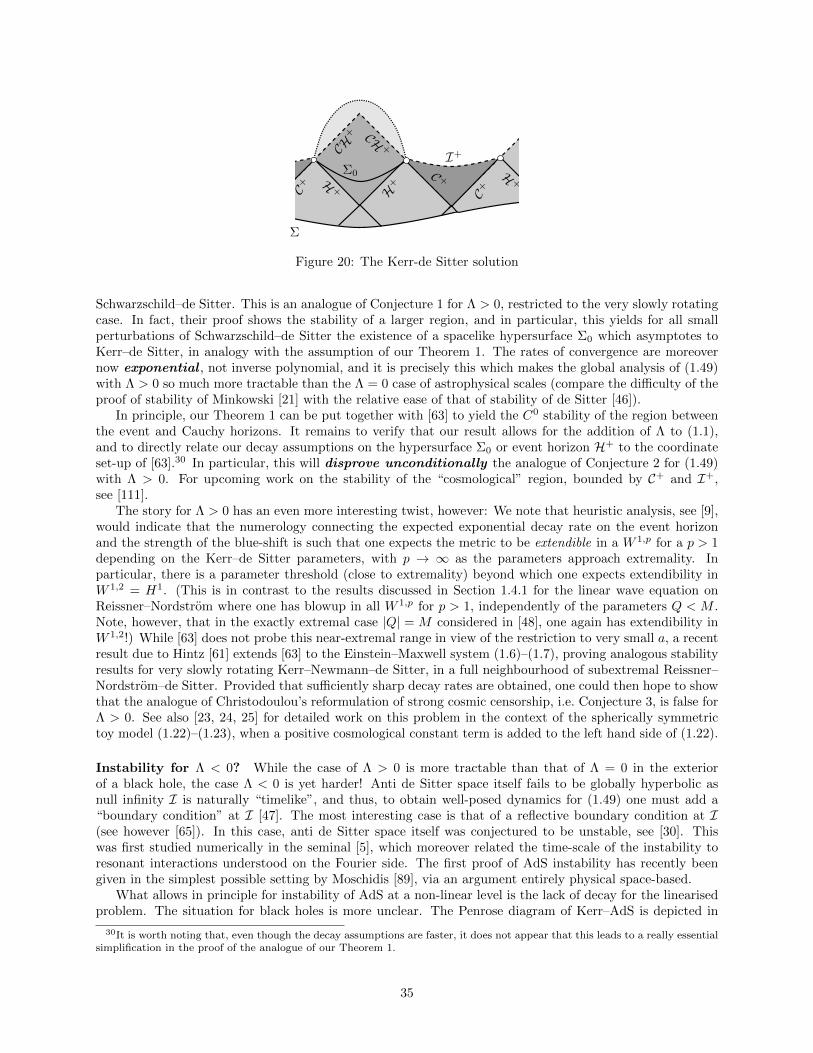
Σ

C +

CH+

H +

I+

H +

CH +

H+C+ C+

Σ0

Figure 20: The Kerr-de Sitter solution

Schwarzschild–de Sitter. This is an analogue of Conjecture 1 for Λ > 0, restricted to the very slowly rotatingcase. In fact, their proof shows the stability of a larger region, and in particular, this yields for all smallperturbations of Schwarzschild–de Sitter the existence of a spacelike hypersurface Σ0 which asymptotes toKerr–de Sitter, in analogy with the assumption of our Theorem 1. The rates of convergence are moreovernow exponential , not inverse polynomial, and it is precisely this which makes the global analysis of (1.49)with Λ > 0 so much more tractable than the Λ = 0 case of astrophysical scales (compare the difficulty of theproof of stability of Minkowski [21] with the relative ease of that of stability of de Sitter [46]).

In principle, our Theorem 1 can be put together with [63] to yield the C0 stability of the region betweenthe event and Cauchy horizons. It remains to verify that our result allows for the addition of Λ to (1.1),and to directly relate our decay assumptions on the hypersurface Σ0 or event horizon H+ to the coordinateset-up of [63].30 In particular, this will disprove unconditionally the analogue of Conjecture 2 for (1.49)with Λ > 0. For upcoming work on the stability of the “cosmological” region, bounded by C+ and I+,see [111].

The story for Λ > 0 has an even more interesting twist, however: We note that heuristic analysis, see [9],would indicate that the numerology connecting the expected exponential decay rate on the event horizonand the strength of the blue-shift is such that one expects the metric to be extendible in a W 1,p for a p > 1depending on the Kerr–de Sitter parameters, with p → ∞ as the parameters approach extremality. Inparticular, there is a parameter threshold (close to extremality) beyond which one expects extendibility inW 1,2 = H1. (This is in contrast to the results discussed in Section 1.4.1 for the linear wave equation onReissner–Nordstrom where one has blowup in all W 1,p for p > 1, independently of the parameters Q < M .Note, however, that in the exactly extremal case |Q| = M considered in [48], one again has extendibility inW 1,2!) While [63] does not probe this near-extremal range in view of the restriction to very small a, a recentresult due to Hintz [61] extends [63] to the Einstein–Maxwell system (1.6)–(1.7), proving analogous stabilityresults for very slowly rotating Kerr–Newmann–de Sitter, in a full neighbourhood of subextremal Reissner–Nordstrom–de Sitter. Provided that sufficiently sharp decay rates are obtained, one could then hope to showthat the analogue of Christodoulou’s reformulation of strong cosmic censorship, i.e. Conjecture 3, is false forΛ > 0. See also [23, 24, 25] for detailed work on this problem in the context of the spherically symmetrictoy model (1.22)–(1.23), when a positive cosmological constant term is added to the left hand side of (1.22).

Instability for Λ < 0? While the case of Λ > 0 is more tractable than that of Λ = 0 in the exteriorof a black hole, the case Λ < 0 is yet harder! Anti de Sitter space itself fails to be globally hyperbolic asnull infinity I is naturally “timelike”, and thus, to obtain well-posed dynamics for (1.49) one must add a“boundary condition” at I [47]. The most interesting case is that of a reflective boundary condition at I(see however [65]). In this case, anti de Sitter space itself was conjectured to be unstable, see [30]. Thiswas first studied numerically in the seminal [5], which moreover related the time-scale of the instability toresonant interactions understood on the Fourier side. The first proof of AdS instability has recently beengiven in the simplest possible setting by Moschidis [89], via an argument entirely physical space-based.

What allows in principle for instability of AdS at a non-linear level is the lack of decay for the linearisedproblem. The situation for black holes is more unclear. The Penrose diagram of Kerr–AdS is depicted in

30It is worth noting that, even though the decay assumptions are faster, it does not appear that this leads to a really essentialsimplification in the proof of the analogue of our Theorem 1.

35

Σ

CH+ CH +

H+ II H +

Figure 21: The Kerr–AdS solution

Figure 21. Holzegel–Smulevici [66, 67] have shown that while solutions of the linear wave equation on Kerr–AdS indeed decay, the rate of decay is only logarithmic, and this slow decay is moreover in general sharp.One scenario is that at the non-linear level, backreaction builds up, and Kerr–AdS shares the unstable fateof pure AdS, and thus the picture of an event horizon settling down to Kerr–AdS is generically not realised.If this is the case, then all bets are off regarding the validity of either weak or strong cosmic censorship!Alternatively, however, the linear picture of slow logarithmic decay could survive in the full non-linear theory,as is suggested in [40]. The latter situation would mean that the proper setting for understanding black holeinteriors in Λ < 0 requires that we replace the assumption of Theorem 1 or 2 with an assumption of dataon Σ0 or H+ logarithmically approaching that of Kerr–AdS in a suitable sense. Now, it would appear thatsuch a slow logarithmic decay does not allow for our stability mechanism, for which it seems essential thatone can prove weighted estimates with polynomial weights in u, as in the quantities (1.39)–(1.40). See alsothe discussion in [4]. Perversely, could this “worse” event horizon behaviour be sufficient to ensure that theoriginal C0 formulation of cosmic censorship (Conjecture 2) becomes true after all for Λ < 0?

We leave such musings for another occasion!

1.7 Acknowledgments

M. D. is supported by NSF grant DMS-1709270 as well as an EPSRC programme grant EP/K00865X/1.J. L. is supported by a Sloan fellowship, a Terman fellowship, and NSF grant DMS-1709458. Much of thisresearch was conducted when J. L. was at the University of Cambridge. The authors thank DemetriosChristodoulou for suggesting this problem many years ago and for many conversations over the years.

2 Spacetimes covered by double null foliations

In this section, we will derive the structure equations satisfied by a spacetime (U , g) globally foliated by adouble null foliation intersecting on spheres. We will not require here the metric g to satisfy the Einsteinequations.

We begin in Section 2.1 with the basic assumptions on the underlying manifold U and metric in explicitform. We shall then show in Section 2.2 that the geometrical interpretation of these assumptions isequivalent to the existence of a natural double null foliation; importantly, this allows us to find appropriateregions of a general spacetime which allow for parametrisation as (U , g). In Section 2.3, we introduce theRicci coefficients and curvature components with respect to a natural null frame associated to the doublenull foliation, and collect several basic facts about them. Finally, in Section 2.4, we describe how the workof Pretorius–Israel [103] implies that that Kerr interior can indeed be parametrised as (U , g).

2.1 The general class of spacetimes

We will introduce here the general class of spacetimes (U , g) we will be considering in this paper. The classof spacetimes is sufficiently general so as to include the Kerr interior and as well as the spacetimes that weconstruct31 in Theorem 1.

31In fact, it will include both the full spacetimes in Theorem 1, as well as appropriate subsets thereof that we consider in thecontext of the bootstrap argument.

36

In Section 2.1.1, we will define the underlying manifold U , followed by the metric and time orientationin Section 2.1.2. We will define an associated null frame in Section 2.1.3.

2.1.1 The differential structure

Let us denote by u and u the standard Euclidean coordinates on R2, and let W ⊂ R2 be a connected opensubset, and let S2 denote the standard unit sphere, with local coordinates θA where A = 1, 2. We define thesmooth manifold U =W × S2.

We can consider (u, u, θ1, θ2) as local coordinates on U .

2.1.2 The metric and time-orientation

Let γ : W → Γ(T ∗S2 × T ∗S2) denote a Riemannian metric on S2, let b : W → Γ(TS2) denote a vector fieldon S2, and let Ω :W → Γ(S2 × R) denote a positive function, all depending smoothly on W.

We can denote the components of b and γ with respect to the local coordinates θA by bA and γAB .These choices induce a Lorentzian metric on U defined by:

g = −2Ω2(du⊗ du+ du⊗ du) + γAB(dθA − bAdu)⊗ (dθB − bBdu). (2.1)

We time-orient the above by requiring that du and du are future directed. With this choice, (U , g) is asmooth 4-dimensional spacetime.

2.1.3 Frames and metric components

Let ∂∂u , ∂

∂u , ∂∂θA

be coordinate vector fields defined with respect to the (u, u, θ1, θ2) coordinate system that

we introduced above.Define the vector fields

L =∂

∂u+ bA

∂

∂θA, L =

∂

∂u. (2.2)

These are easily seen to be globally defined null vector fields on U . We can in fact write L = −2Ω2Du,L = −2Ω2Du, where D denotes the gradient with respect to (2.1).

These vector fields satisfy the properties

Lu = Lu = 0, Lu = Lu = 1. (2.3)

We have

g(L,L) = −2Ω2, g(L,∂

∂θA) = g(L,

∂

∂θA) = g(L,L) = g(L,L) = 0,

γAB.= g(

∂

∂θA,∂

∂θB).

As a consequence, the inverse metric g−1 is given by

g−1 = − 1

2Ω2(L⊗ L+ L⊗ L) + γ−1.

The inverse metric g−1 has the following non-vanishing components:

(g−1)AB = (γ−1)AB , (g−1)uu = − 1

2Ω2, (g−1)uA = − 1

2Ω2bA,

the remaining components being zero.We define L′ and L′ as the following null vector fields

L′.= −2Du = Ω−2 ∂

∂u, L′

.= −2Du = Ω−2

(∂

∂u+ bA

∂

∂θA

). (2.4)

It is easy to check that L′ and L′ are geodesic, i.e.

DL′L′ = DL′L

′ = 0. (2.5)

37

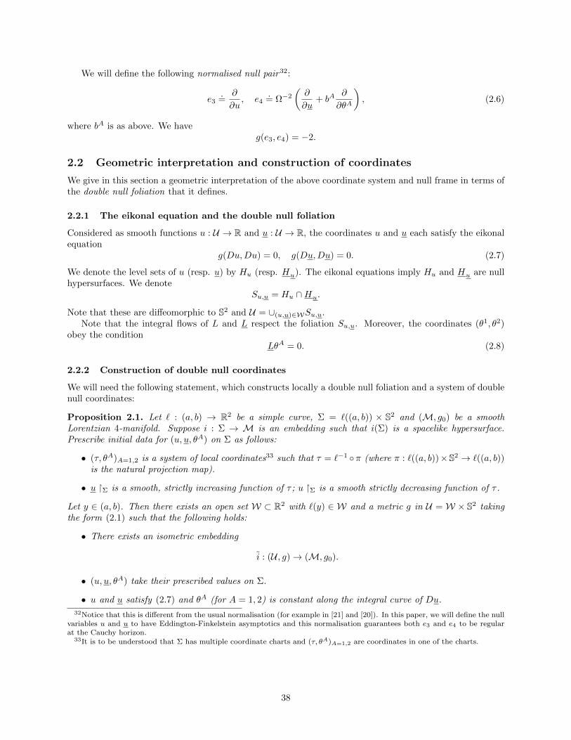
We will define the following normalised null pair32:

e3.=

∂

∂u, e4

.= Ω−2

(∂

∂u+ bA

∂

∂θA

), (2.6)

where bA is as above. We haveg(e3, e4) = −2.

2.2 Geometric interpretation and construction of coordinates

We give in this section a geometric interpretation of the above coordinate system and null frame in terms ofthe double null foliation that it defines.

2.2.1 The eikonal equation and the double null foliation

Considered as smooth functions u : U → R and u : U → R, the coordinates u and u each satisfy the eikonalequation

g(Du,Du) = 0, g(Du,Du) = 0. (2.7)

We denote the level sets of u (resp. u) by Hu (resp. Hu). The eikonal equations imply Hu and Hu are nullhypersurfaces. We denote

Su,u = Hu ∩Hu.

Note that these are diffeomorphic to S2 and U = ∪(u,u)∈WSu,u.Note that the integral flows of L and L respect the foliation Su,u. Moreover, the coordinates (θ1, θ2)

obey the conditionLθA = 0. (2.8)

2.2.2 Construction of double null coordinates

We will need the following statement, which constructs locally a double null foliation and a system of doublenull coordinates:

Proposition 2.1. Let ` : (a, b) → R2 be a simple curve, Σ = `((a, b)) × S2 and (M, g0) be a smoothLorentzian 4-manifold. Suppose i : Σ → M is an embedding such that i(Σ) is a spacelike hypersurface.Prescribe initial data for (u, u, θA) on Σ as follows:

• (τ, θA)A=1,2 is a system of local coordinates33 such that τ = `−1 π (where π : `((a, b))×S2 → `((a, b))is the natural projection map).

• u Σ is a smooth, strictly increasing function of τ ; u Σ is a smooth strictly decreasing function of τ .

Let y ∈ (a, b). Then there exists an open set W ⊂ R2 with `(y) ∈ W and a metric g in U = W × S2 takingthe form (2.1) such that the following holds:

• There exists an isometric embedding

i : (U , g)→ (M, g0).

• (u, u, θA) take their prescribed values on Σ.

• u and u satisfy (2.7) and θA (for A = 1, 2) is constant along the integral curve of Du.

32Notice that this is different from the usual normalisation (for example in [21] and [20]). In this paper, we will define the nullvariables u and u to have Eddington-Finkelstein asymptotics and this normalisation guarantees both e3 and e4 to be regularat the Cauchy horizon.

33It is to be understood that Σ has multiple coordinate charts and (τ, θA)A=1,2 are coordinates in one of the charts.

38

Proof. According to Section 2.2.1, the key is to solve (2.7), which can in turn be achieved by solving thegeodesic equation. More precisely, given the initial data for (u, u, θA) as above, we prescribe the initial data34

L′ Σ=2

(−nu)(N + n), L′ Σ=

2

nu(N − n).

where n is the unique unit normal in Σ to the constant-τ satisfying nτ > 0, and N is unique future directedunit normal to Σ.

We then solve the following system of equations: L′ and L′ satisfy the geodesic equation, and (u, u, θA)satisfy transport equations:

DL′L′ = DL′L

′ = 0, L′u = L u = 0, LθA = 0.

The existence of a solution (L′, L′, u, u, θA) follows from compactness and standard local existence theoryfor odes.

It can then be checked that for such a solution, u and u satisfy the eikonal equation (2.7). In view of thediscussions in Section 2.2.1, this then implies the conclusion of the proposition.

2.3 Computations

2.3.1 Derivatives and connections

Before we proceed, it is convenient to introduce the convention that lower case Greek letter µ, ν, etc. arespacetime indices, while capital Latin indices A, B, C, etc. are indices for the 2-spheres Su,u, i.e. they runthrough 1 and 2. Unless otherwise stated, repeated indices will be summed over.

We denote the spacetime covariant derivative with respect to the Levi–Civita connection associated to gby D. We compute a subset of the spacetime Christoffel symbols (which we will denote using boldface Γ),which will be useful below:

ΓABu =1

2(γ−1)AC

∂

∂uγBC ,

ΓABu =1

2(γ−1)AC(

∂

∂uγBC −

∂

∂θB(γCDb

D) +∂

∂θC(γBDb

D)) +1

4Ω2bA(2

∂

∂θBΩ2 − ∂

∂u(γBCb

C)),

ΓABC =1

2(γ−1)AD(− ∂

∂θDγBC +

∂

∂θBγCD +

∂

∂θCγBD) +

1

4Ω2bA

∂

∂uγBC ,

ΓuAu = 0,

ΓuAu = − 1

4Ω2(2

∂

∂θAΩ2 − ∂

∂u(γABb

B)),

ΓuAB =

1

4Ω2

∂

∂uγAB .

For the remainder of the paper, we will frequently consider tensor fields which are tangential to thespheres Su,u (or simply, S-tangent), i.e. tensorfields of the form

φ = φB1...BsA1...Ar

dθA1 ⊗ · · · ⊗ dθAr ⊗ ∂

∂θB1⊗ · · · ⊗ ∂

∂θBs.

We define the differential operators /∇, /∇3 and /∇4, which act on these S-tangent vector fields:

Definition 2.2. We denote by /∇ the Levi–Civita connection35 induced by the metric γ on Su,u and by /∇3,/∇4 the projections to Su,u of the covariant derivatives D3 = De3 , D4 = De4 .

34Note that the coefficients in the initial data for L′ and L′ are chosen to follow the notation introduced in (2.4). Indeed,since

L′u Σ= 0 =⇒ Nu = −nu,it follows that

Du Σ= −(Nu)N + (nu)n = (nu)(N + n) = −1

2L′ Σ .

Similarly for L′.35We note that using the above calculations for the spacetime Christoffel symbols, the induced covariant derivative operator

coincides with the projection of the spacetime covariant derivatives to the tangent space of Su,u.

39

We now apply the above calculations for Γ to derive the expressions for /∇, /∇3 and /∇4 in coordinates.First, the formula for /∇ is standard: for every tensor φ of rank r tangential to the spheres Su,u, /∇BφA1A2...Ar

is a tensor of rank r + 1 tangential to the spheres Su,u given by

/∇BφA1A2...Ar =∂

∂θBφA1A2...Ar −

r∑i=1

/ΓCAiBφA1...AiC...Ar

, (2.9)

where Ai denotes that the Ai which was originally present is removed.

/ΓCDE =

1

2(γ−1)CF (

∂

∂θDγEF +

∂

∂θEγDF −

∂

∂θFγDE). (2.10)

To derive the expressions for /∇3 and /∇4, it is convenient for later reference to introduce the null secondfundamental forms as a covariant 2-tensor tangential to the 2-spheres Su,u by

χAB = g(D ∂

∂θAe4,

∂

∂θB), χ

AB= g(D ∂

∂θAe3,

∂

∂θB). (2.11)

In the double null coordinate system, for every tensor φ of rank r tangential to the spheres Su,u, we have

/∇3φA1A2...Ar

=∂

∂uφA1A2...Ar −

r∑i=1

(ΓBAiu − bBΓ

uAiu

)φA1...AiB...Ar

=∂

∂uφA1A2...Ar −

r∑i=1

(γ−1)BCχAiC

φA1...AiB...Ar.

(2.12)

/∇4 can be expressed in the double null coordinate system as

/∇4φA1A2...Ar

=Ω−2(∂

∂u+ bC

∂

∂θC)φA1A2...Ar −

r∑i=1

Ω−2(ΓBAiu + bCΓBAiC − bBΓ

uAiu− bBbCΓ

uAiC

)φA1...AiB...Ar

=Ω−2(∂

∂u+ bC

∂

∂θC)φA1A2...Ar −

r∑i=1

((γ−1)BCχAiC − Ω−2 ∂

∂θAibB)φA1...AiB...Ar

.

(2.13)

We can directly check by using the above formula that

/∇γ = 0, /∇3γ = /∇4γ = 0. (2.14)

Moreover, for χ and χ as in (2.11), we have the first variation formulae

L/ Lγ = 2Ω2χ, L/ Lγ = 2χ, (2.15)

where L/ L denotes the restriction of the Lie derivative to TSu,u (See [20], Chapter 1).We end this subsection with the definitions of a few more differential operators on tensors tangential

to Su,u which will be useful for later use. For totally symmetric tensors φ of rank r + 1, the /div and /curloperators are defined by the formulas

( /div φ)A1...Ar.= (γ−1)BC /∇BφCA1...Ar , (2.16)

( /curl φ)A1...Ar.=∈BC /∇BφCA1...Ar . (2.17)

For a scalar function φ, define /∆ to be the Laplace–Beltrami operator associated to the metric γ, i.e.

/∆φ.= (γ−1)AB /∇A /∇Bφ. (2.18)

Finally, define the operator /∇⊗ on a 1-form φA by

( /∇⊗φ)AB.= /∇AφB + /∇BφA − γAB /div φ. (2.19)

40

2.3.2 Ricci coefficients and null curvature components

As before, we use capital Latin indices A,B to denote 1, 2, which are indices on the spheres Su,u. LettingeA = ∂

∂θAfor A = 1, 2, we define the Ricci coefficients relative to e1, e2, e3, e4. These can be viewed as

tensor fields tangent to Su,u, the 2-spheres adapted to the double null foliation. Let

χAB.= g(DAe4, eB), χ

AB

.= g(DAe3, eB),

ηA.= −1

2g(D3eA, e4), η

A

.= −1

2g(D4eA, e3),

ω.= −1

4g(D4e3, e4), ω

.= −1

4g(D3e4, e3),

ζA.=

1

2g(DAe4, e3),

(2.20)

where DA = DeA , D3 = De3 and D4 = De4 . It is clear from the definitions that these Ricci coefficients areof different rank, namely that χ and χ are symmetric 2-tensors, η, η and ζ are 1-forms and ω and ω arescalars.

We also introduce the null curvature components as follows:

αAB.= R(eA, e4, eB , e4), αAB

.= R(eA, e3, eB , e3),

βA.=

1

2R(eA, e4, e3, e4), β

A

.=

1

2R(eA, e3, e3, e4),

ρ.=

1

4R(e4, e3, e4, e3), σ

.=

1

4∗R(e4, e3, e4, e3).

(2.21)

Here, R is the Riemann curvature tensor of g, given by

R(X,Y, Z,W ).= −g(DXDY Z −DYDXZ,W ),

and ∗R denotes the Hodge dual of R given by36

∗Rµνλσ.= εµναβR

αβλσ,

where ε is the volume form of (U , g). As the Ricci coefficients, the null curvature components are also tensorfields tangent to Su,u. It is easy to see that α and α are symmetric 2-tensors, βA and β

Aare 1-forms and ρ,

σ are scalars.For the null second fundamental forms χAB and χ

AB, we also use χAB and χ

ABto denote their respective

traceless parts, i.e.

χAB.= χAB −

1

2(/trχ)γAB , χ

AB

.= χAB −

1

2(/trχ)γAB , (2.22)

where /trχ and /trχ denote the trace of the null second fundamental forms with respect to γ, i.e.

/trχ.= (γ−1)ABχAB , /trχ

.= (γ−1)ABχ

AB. (2.23)

As we will see later, it will be convenient to also introduce two more scalars related to curvature37. First,we use K to denote the Gauss curvature of the 2-surface Su,u adapted to the double null foliation, i.e.

γBCK =∂

∂θA/ΓABC −

∂

∂θC/ΓABA + /Γ

AAD/Γ

DBC − /Γ

ACD/Γ

DBA, (2.24)

where /Γ is as in (2.10). We also define

σ.= σ +

1

2∈AB (γ−1)CDχ

ACχBD (2.25)

36Recall that Greek indices denote spacetime indices.37These are the renormalised curvature components; see Sections 1.5.3 and 3.1.

41

where ∈ is the volume form associated to the metric γ. The importance of K and σ is that together withβ and β, they form a set of renormalised null curvature components. They behave better than general nullcurvature components and play a fundamental role in our argument, cf. Section 1.5.3.

In anticipation of the top order estimates38, we introduce three scalars, which are special combinationsof angular covariant derivatives of the Ricci coefficients and the curvature components (or their derivatives).Define39

µ.= − /div η +K, µ

.= − /div η +K, ω/

.= /∆ω +

1

2/div β. (2.26)

2.3.3 Some basic identities

For the Su,u-tangent covariant tensor fields defined in (2.20) and (2.21), when there is no risk of confusion40,we will raise and lower indices with respect to the metric γ on Su,u without further comments.

In the remainder of this subsection, we prove some simple identities for the Ricci coefficients, which holdbecause of our choice of the normalisation of e3 and e4 in (2.6). In Proposition 2.3, we prove some relationsbetween the Ricci coefficients and in Proposition 2.4 we will relate the Ricci coefficients and the metriccomponents defined in Section 2.1.1.

Proposition 2.3. In the gauge given by (2.6), we have41

ω = 0, ω = − /∇3(log Ω),

ζA = ηA, /∇A(log Ω) =1

2(ηA + η

A).

(2.27)

Proof. The first equality follows immediately from the fact that e4 is geodesic, i.e.

ω = −1

4g(D4e3, e4) =

1

4g(e3, D4e4) = 0.

For the second equality, we use the fact that Ω−2e3 is geodesic to get

ω = −1

4g(D3e4, e3) =

1

4g(e4, D3(Ω2Ω−2e3)) =

1

4(e3Ω2)Ω−2g(e3, e4) = −(e3 log Ω).

Since e3 = ∂∂u and eA = ∂

∂θA, we have g([e3, eA], e4) = 0. Therefore,

ηA = −1

2g(D3eA, e4) = −1

2g(DAe3, e4) =

1

2g(DAe4, e3) = ζA.

Finally, since e4 = 1Ω2 ( ∂

∂u + bA ∂∂θA

) and eA = ∂∂θA

, we have

g([e4, eA], e3) = −(eAΩ−2)Ω2g(e3, e4) = 2(eAΩ−2)Ω2 = −4(eA log Ω).

As a consequence, this implies

ηA

= −1

2g(D4eA, e3) = −1

2g(DAe4, e3)− 1

2g([e4, eA], e3) = −ζA + 2(eA log Ω) = −ηA + 2(eA log Ω).

After rearranging, we obtain

/∇A(log Ω) =1

2(ηA + η

A).

38µ and µ satisfy better estimates than general first angular covariant derivatives of the Ricci coefficients or general curvaturecomponents (similarly, ω/ satisfies better estimates than general second angular covariant derivatives of the Ricci coefficients orgeneral first angular covariant derivatives of curvature components); see Sections 3.3, 7.5 and 7.6. This observation, originatingin [20, 21], will be crucial in Section 11.

39Recall here the notations introduced in (2.16) and (2.18).40As we will see later, we will encounter more than one metric in the proof of our main theorem, in which case we will further

specify the metric with respect to which we raise and lower indices.41Although ω = 0, we will still keep it in the equations below (see Section 3.1) for easy comparison with the formulae found

in the literature where a difference normalisation of e3 and e4 is chosen.

42

We also have the following equations relating the metric components and the Ricci coefficients:

Proposition 2.4. γ satisfies the equations:

∂

∂uγAB = 2χ

AB,

(∂

∂u+ bC

∂

∂θC)γAB + γAC

∂

∂θBbC + γBC

∂

∂θAbC = 2Ω2χAB .

Ω verifies the equation:∂

∂ulog Ω = −ω.

bA satisfies the following equation:

∂bA

∂u= 2Ω2(ηA − ηA) = 4Ω2(ζA − /∇A log Ω).

Proof. The equation for γ follows from (2.15) and the equation for Ω is derived in (2.27). Finally, recall from(2.6) that

e3 =∂

∂u, e4 = Ω−2

(∂

∂u+ bA

∂

∂θA

).

Therefore,

[e3, e4] = (∂

∂uΩ−2)Ω2e4 + Ω−2 ∂b

A

∂u

∂

∂θA.

As a consequence,

Ω−2γAB∂bB

∂u=g([e3, e4], eA) = g(D3e4, eA)− g(D4e3, eA)

=− g(D3eA, e4) + g(D4eA, e3) = 2ηA − 2ηA.

The conclusion follows from combining this with (2.27).

2.4 Kerr interior in double null foliation

As we mentioned in the beginning of Section 2.1, the interior of the Kerr spacetime can be put into the formof the general class of spacetime that we consider. In other words, there exists a global double null foliationin the Kerr interior. This fact is a consequence of [103]. Detailed discussions of the double null foliation inthe Kerr interior, as well as many calculations and proofs, are deferred to Appendix A. Here, however, wegather a few facts which will be repeatedly used in the proof of the main theorem.

Fix M, a ∈ R with 0 < |a| < M . The Kerr interior (MKerr, ga,M ) with mass M and specific angularmomentum a is a spacetime whereMKerr = R2×S2 and the metric ga,M in the Boyer–Lindquist coordinates(t, r, θ, φ) takes the form (A.1). Here, t ∈ R, r ∈ (r−, r+), θ ∈ (0, π) and φ ∈ [0, 2π), where r± = M ±√M2 − a2 are the roots of ∆ = r2 + a2 − 2Mr.

The Kerr interior (MKerr, ga,M ) admits a global double null foliation so that in an appropriate doublenull coordinate system, the metric inMKerr = R2×S2 takes the form as in the class of spacetimes describedin Section 2.1. More precisely, ga,M can be written as

ga,M = −2Ω2K(du⊗ du+ du⊗ du) + (γK)AB(dθA − (bK)Adu)⊗ (dθB − (bK)Bdu).

where42 ΩK, γK and bK are given in (A.43) (and expressions in (A.43) are functions of (u, u, θ1, θ2) and aredefined implicitly in Sections A.1 and A.4).

The following are some facts regarding the Kerr metric in this coordinate system that are useful in theremaining of this paper:

42Note that in Appendix A, the metric is given so that a set of spherical-like coordinates are used on the 2-spheres. Therefore,the local coordinate system (u, u, θ1, θ2) misses the two points on the rotation axis on every S2. Nevertheless, it is easy to checkthat one can introduce regular coordinates there.

43

• (Event and Cauchy horizons) Upon appropriate change of coordinates (both rescaling the null u andu coordinates and rotating the angular coordinates), one can attach appropriate boundaries toMKerr

and define the event horizon and Cauchy horizon. The metric moreover extends smoothly up to theevent and Cauchy horizons. See Section A.5.

• (Behaviour of the metric components) ΩK is degenerate as u, u→ ±∞ and in fact obeys the followingbounds in the region43 (u, u) : u + u ≥ CR, u ≤ −1 × S2 for any fixed CR ∈ R (see Figure 24 inAppendix A for a depiction of this subset)

e− r+−r−r2−+a2 (u+u)

.CR Ω2K .CR e

− r+−r−r2−+a2 (u+u)

,

while γK and bK are globally bounded and have non-vanishing limits as u, u → ±∞. As before,here, r± = M ±

√M2 − a2. Moreover, the angular coordinate partial derivatives of Ω2

K and γK havesimilar behaviour, and the angular coordinate partial derivatives of bK is degenerate as u, u → ±∞(see Propositions A.12, A.14 and A.15).

• (Estimates for the Ricci coefficients) For any CR ∈ R and I ∈ N, in (u, u) : u+u ≥ CR, u ≤ −1×S2,the Ricci coefficients satisfy the following estimates (see Definition A.13 and Proposition A.19)∑

0≤i≤I

(|( /∇K)iχK|γK + |( /∇K)iηK|γK + |( /∇K)iηK|γK) .CR,I 1,

∑0≤i≤I

|( /∇K)i(ωK −1

2

r+ − r−r2− + a2

)|γK +∑

0≤i≤I

|( /∇K)iχK|γK .CR,I e− r+−r−r2−+a2 (u+u)

.

• (Estimates for the renormalised null curvature components) For any CR ∈ R and I ∈ N, in (u, u) :u+u ≥ CR, u ≤ −1× S2, the renormalised null curvature components satisfy the following estimates(see Definition A.13, Propositions A.21 and A.23)

∑0≤i≤I

|( /∇K)iβK|γK .CR,I e− r+−r−r2−+a2 (u+u)

,∑

0≤i≤I

(|( /∇K)iσK|γK + |( /∇K)iKK|γK) .CR,I 1,

∑0≤i≤I

|( /∇K)iβK|γK .CR,I 1.

Further elaboration of these statements, as well as their proofs, can all be found Appendix A. In additionto the facts listed above, there are a number of other results regarding the Kerr interior in the double nullfoliation gauge that we will use in the remainder of the paper. For all those results, we will also refer thereader to Appendix A.

3 Equations in the double null foliation and the schematic nota-tion

In this section, we derive consequences of the Einstein vacuum equations under the geometric setup intro-duced in Section 2. From now on, we consider a spacetime (U , g) (with U =W × S2 and W ⊂ R2) where gtakes the form (2.1). Assume that (U , g) satisfies the Einstein vacuum equations (1.1). We will recast (1.1)as a system for Ricci coefficients and null curvature components (recall the definition from (2.20) and (2.21)in Section 2.3.2).

In Section 3.1, we will write down the arising system for Ricci coefficients and null curvature components.As we have discussed earlier, for most of this paper, the exact form of the terms in the equations will notbe too important. Instead, for most of the nonlinear terms, it suffices to understand the “null structure”

43We especially highlight this region since the present paper is exactly concerned with perturbations of the Kerr spacetimein this region.

44

hidden in the equations. For this reason, we introduce a schematic notation in Section 3.2 so as to simplifythe exposition and to emphasise the structures of the equations that we need (cf. Sections 1.5.3, 1.5.4 and[80]). We end the section by writing down the equations in schematic form in Section 3.3.

Let us already note here that the schematic notation introduced in this section will be further developedlater in Section 7.1, cf. Section 1.5.4.

3.1 Equations

Before writing down the equations, we need to introduce a few more notations. First, for S-tangent tensorfields, we define the following conventions for contraction with respect to the metric γ:

φ(1) · φ(2) .= (γ−1)AC(γ−1)BDφ

(1)ABφ

(2)CD for symmetric 2-tensors φ

(1)AB , φ

(2)AB ,

φ(1) · φ(2) .= (γ−1)ABφ

(1)A φ

(2)B for 1-forms φ

(1)A , φ

(2)A ,

(φ(1) · φ(2))A.= (γ−1)BCφ

(1)ABφ

(2)C for a symmetric 2-tensor φ

(1)AB and a 1-form φ

(2)A ,

(φ(1)⊗φ(2))AB.= φ

(1)A φ

(2)B + φ

(1)B φ

(2)A − γAB((γ−1)CDφ

(1)C φ

(2)D ) for one forms φ

(1)A , φ

(2)A ,

φ(1) ∧ φ(2) .=∈AB (γ−1)CDφ

(1)ACφ

(2)BD for symmetric two tensors φ

(1)AB , φ

(2)AB ,

where ∈ is the volume form associated to the metric γ. Define ∗ of 1-forms and symmetric 2-tensorsrespectively as follows (note that on 1-forms this is the Hodge dual on Su,u):

∗φA.=γAC ∈CB φB ,

∗φAB.= γBD ∈DC φAC .

Define also the trace for totally symmetric tensors of rank r to be

( /tr φ)A1...Ar−1

.= (γ−1)BCφBCA1...Ar−1

. (3.1)

We now write down the equations. For this it is useful to recall the definitions (2.16), (2.17) and (2.19).First, after separating into their trace and traceless parts (cf. (2.22) and (2.23)), χ and χ satisfy the followingnull structure equations:

/∇4 /trχ+1

2(/trχ)2 = −|χ|2 − 2ω /trχ,

/∇4χ+ /trχχ = −2ωχ− α,

/∇3 /trχ+1

2(/trχ)2 = −2ω /trχ− |χ|2,

/∇3χ+ /trχ χ = −2ωχ− α,

/∇4 /trχ+1

2/trχ/trχ = 2ω /trχ+ 2ρ− χ · χ+ 2 /div η + 2|η|2,

/∇4χ+1

2/trχχ = /∇⊗η + 2ωχ− 1

2/trχχ+ η⊗η,

/∇3 /trχ+1

2/trχ/trχ = 2ω /trχ+ 2ρ− χ · χ+ 2 /div η + 2|η|2,

/∇3χ+1

2/trχχ = /∇⊗η + 2ωχ− 1

2/trχχ+ η⊗η.

(3.2)

The other Ricci coefficients satisfy the following null structure equations:

/∇4η = −χ · (η − η)− β,/∇3η = −χ · (η − η) + β,

/∇3ω + /∇4ω = 4ωω + ζ · (η − η)− η · η + ρ.

(3.3)

In our choice of gauge, since ω = 0 (see (2.27)), the last equation in (3.3) reduces to the following equationfor ω:

/∇4ω = ζ · (η − η)− η · η + ρ. (3.4)

45

The Ricci coefficients also satisfy the following constraint equations:

/div χ =1

2/∇/trχ− ζ · (χ− /trχγ)− β,

/div χ =1

2/∇/trχ+ ζ · (χ− /trχγ) + β,

/curl η = − /curl η = σ +1

2χ ∧ χ,

K = −ρ+1

2χ · χ− 1

4/trχ/trχ.

(3.5)

where we recall again that K is the Gauss curvature of the spheres Su,u. The null curvature componentssatisfy the following null Bianchi equations:

/∇3α+1

2/trχα = /∇⊗β + 4ωα− 3(χρ+∗ χσ) + (ζ + 4η)⊗β,

/∇4β + 2/trχβ = /div α− 2ωβ + (2ζ + η) · α,/∇3β + /trχβ = /∇ρ+ 2ωβ +∗ /∇σ + 2χ · β + 3(ηρ+∗ ησ),

/∇4σ +3

2/trχσ = − /div

∗β +

1

2χ ∧ α− ζ ∧ β − 2η ∧ β,

/∇3σ +3

2/trχσ = − /div

∗β − 1

2χ ∧ α+ ζ ∧ β − 2η ∧ β,

/∇4ρ+3

2/trχρ = /div β − 1

2χ · α+ ζ · β + 2η · β,

/∇3ρ+3

2/trχρ = − /div β − 1

2χ · α+ ζ · β − 2η · β,

/∇4β + /trχβ = − /∇ρ+∗ /∇σ + 2ωβ + 2χ · β − 3(ηρ−∗ ησ),

/∇3β + 2/trχβ = − /div α− 2ωβ − (−2ζ + η) · α,

/∇4α+1

2/trχα = − /∇⊗β + 4ωα− 3(χρ−∗ χσ) + (ζ − 4η)⊗β.

(3.6)

We now rewrite the Bianchi equations in terms of the renormalised null curvature components, i.e. wewill use the Gauss curvature K of the spheres Su,u and the renormalised null curvature component σ definedin (2.25) instead of ρ and σ. Notice that with the notation that has now been introduced, we can write

σ = σ +1

2χ ∧ χ.

Recall again that one of the main challenges of the problem in this paper is the potential null singularityat the Cauchy horizon. In [80], where the local existence problem for null singularities was treated, it wascrucial that the null curvature components ρ and σ were eliminated in favor of K and σ (cf. Section 1.5.3).The use of these renormalised null curvature components will also be important in this paper.

46

The (renormalised) Bianchi equations take the following form:

/∇3β + /trχβ =− /∇K +∗ /∇σ + 2ωβ + 2χ · β − 3(ηK −∗ ησ) +1

2( /∇(χ · χ) +∗ /∇(χ ∧ χ))

+3

2(ηχ · χ+∗ ηχ ∧ χ)− 1

4( /∇/trχ/trχ+ /trχ/∇/trχ)− 3

4η /trχ/trχ,

/∇4σ +3

2/trχσ =− /div

∗β − ζ ∧ β − 2η ∧ β − 1

2χ ∧ ( /∇⊗η)− 1

2χ ∧ (η⊗η),

/∇4K + /trχK =− /div β − ζ · β − 2η · β +1

2χ · /∇⊗η +

1

2χ · (η⊗η)− 1

2/trχ /div η − 1

2/trχ|η|2,

/∇3σ +3

2/trχσ =− /div

∗β + ζ ∧ β − 2η ∧ β +

1

2χ ∧ ( /∇⊗η) +

1

2χ ∧ (η⊗η),

/∇3K + /trχK = /div β − ζ · β + 2η · β +1

2χ · /∇⊗η +

1

2χ · (η⊗η)− 1

2/trχ /div η − 1

2/trχ|η|2,

/∇4β + /trχβ = /∇K +∗ /∇σ + 2ωβ + 2χ · β + 3(ηK +∗ ησ)− 1

2( /∇(χ · χ)−∗ /∇(χ ∧ χ))

+1

4( /∇/trχ/trχ+ /trχ/∇/trχ)− 3

2(ηχ · χ−∗ ηχ ∧ χ) +

3

4η /trχ/trχ.

(3.7)

Notice that we have obtained a system for the renormalised null curvature components in which the nullcurvature components α and α do not appear.44

3.2 Schematic Notation

We introduce a schematic notation for the equations that we consider. We will use the symbol =S toemphasise that an equation is only to be understood schematically.

We first introduce schematic expressions for the Ricci coefficients according to the estimates that theywill eventually be shown to obey. More precisely, let

ψ ∈ η, η, ψH ∈ /trχ, χ, ψH ∈ /trχ, χ.

When writing an equation in the schematic notation, the following conventions will be used:

• (Numerical constants) We use the convention that the exact constants are kept on the left hand sideof =S while we do not keep track45 of the constants on the right hand side of =S.

• (Quantities on left and right hand side) When a schematic quantity, say ψH , appears on the right handside of a schematic equation, one should understand it as summing over all possible ψH ∈ /trχ, χ. Onthe other hand, when a schematic quantity, again say ψH , appears on the left hand side, one shouldunderstand it as representing a fixed ψH ∈ /trχ, χ. For instance, in (3.8) below, the /∇3ψH−2ωψH onthe left hand side is meant to represent either /∇3 /trχ−2ω /trχ or /∇3χ−2ωχ (but not, say, /∇3χ−2ω /trχγ).

• (Contractions with respect to the metric) We will denote by ψψ (or ψψH , etc) an arbitrary contractionwith respect to the metric γ.

• (Derivatives and products) /∇iψj will be used to denote the sum of all terms which are products of j

factors, such that each factor takes the form /∇ikψ and that the sum of all ik’s is i, i.e.

/∇iψj =S

∑i1+i2+...+ij=i

/∇i1ψ /∇i2ψ... /∇ijψ︸ ︷︷ ︸j factors

.

• (The bracket notation) We will use brackets to denote terms with one of the components in the brackets.For instance, the notation ψ(ψ,ψH) denotes the sum of all terms of the form ψψ or ψψH .

44Moreover, compared to the renormalisation in [84], this system do not contain the terms /trχ|χ|2 and /trχ|χ|2 which wouldbe uncontrollable in the context of this paper. This observation already played an important role in [80].

45Obviously, we will use this schematic notation only in situations where the exact constant in front of the term is irrelevantto the argument.

47

• (Extra terms) We will allow in the schematic expression some terms on the right hand side of =S whichare not present in the original equation46. This creates no extra problems since in the proof of thetheorem, we will be bounding all the terms on the right hand side of =S.

• (Rank of the tensor) When using the schematic notation, we suppress the rank of the tensor involved.This will allow us to write schematically the equations for various tensors of different rank in a compactmanner.

• (Norm of a schematic quantity) We will often write |ψ|, |ψH |, etc. to denote the norm of a schematicquantity, which is understood to be taken with respect to γ.

Remark 3.1 (Differentiating the schematic equations). Note that with the conventions we introduced above,we can differentiate the schematic equation without knowing precisely the terms on the right hand side ofthe schematic equation. For instance, if φ =S φ

′, then it holds that /∇φ =S /∇φ′. Similar statements hold forhigher derivatives.

We again remind the reader that we will further develop the above schematic notation in Section 7.1,where we introduce the reduced schematic notations; see also Section 1.5.4.

3.3 Equations in schematic notation

Given the schematic notation introduced in Section 3.2, we now rewrite some of the equations in Section 3.1in schematic form. These include the transport and constraint equations for the Ricci coefficients, as well asthe Bianchi equations for the renormalised null curvature components. In addition, we will write down theschematic transport equations for the quantities we defined in (2.26). (Note that while we do not explicitlywrite down schematic equations for the metric components, in the rest of the paper, we do need to rely onthe equations in (2.14) and Proposition 2.4 satisfied by the metric components.)

The Ricci coefficients ψH satisfy the schematic equation

/∇3ψH − 2ωψH =S K + /∇ψ + ψψ + ψHψH . (3.8)

Here, we recall our convention that (1) all the exact constants are kept on the left hand side of the equalitysign and (2) the ψH on the left hand side refers to the same Ricci coefficient while ψH on the right handside can denote any of ψH ∈ /trχ, χ. The Ricci coefficients ψH similarly obey the schematic

/∇4ψH =S K + /∇ψ + ψψ + ψHψH . (3.9)

In fact, for later applications, it will be useful to note that ψH and ψH obey slightly more precise schematicequations, which we also record here:

/∇3ψH − 2ωψH =S K + /∇η + ψψ + ψHψH , (3.10)

/∇4ψH =S K + /∇η + ψψ + ψHψH . (3.11)

The Ricci coefficients ψ ∈ η, η obey either one of the following schematic equations:

/∇3η − β =S ψψH (3.12)

or/∇4η + β =S ψψH . (3.13)

The Ricci coefficient ω verifies the following schematic equation:

/∇4ω +K =S ψψ + ψHψH . (3.14)

The Codazzi equations, i.e. the first two equations in (3.5), can be expressed schematically as follows:

/div χ+ β =S /∇/trχ+ ψψH , (3.15)

46This should already be apparent in the discussions of “derivatives and products” and “the bracket notation” since we allowthe sum of all terms of a particular form.

48

and/div χ− β =S /∇/trχ+ ψψH . (3.16)

Using the Codazzi equations, we can further simplify the schematic equations (3.12) and (3.13) for η andη to obtain

/∇3η =S

∑i1+i2=1

ψi1 /∇i2ψH (3.17)

and/∇4η =S

∑i1+i2=1

ψi1 /∇i2ψH . (3.18)

We also rewrite the Bianchi equations in the schematic notation:

/∇3β + /∇K −∗ /∇σ − 2ωβ =S

∑i1+i2+i3=1

ψi1 /∇i2ψH /∇i3ψH + ψK +

∑i1+i2=1

ψi1ψ /∇i2ψ,

/∇4σ + /div∗β =S

∑i1+i2+i3=1

ψi1 /∇i2ψ /∇i3ψH ,

/∇4K + /div β =S ψHK +∑

i1+i2+i3=1

ψi1 /∇i2ψ /∇i3ψH ,

/∇3σ + /div∗β =S

∑i1+i2+i3=1

ψi1 /∇i2ψ /∇i3ψH ,

/∇3K − /div β =S ψHK +∑

i1+i2+i3=1

ψi1 /∇i2ψ /∇i3ψH ,

/∇4β − /∇K −∗ /∇σ =S

∑i1+i2+i3=1

ψi1 /∇i2ψH /∇i3ψH + ψK +

∑i1+i2=1

ψi1ψ /∇i2ψ.

(3.19)

Notice that in order to derive the schematic equations in (3.19), we have used the first three equations in(3.5) to express the (renormalised) null curvature components β, β and σ in terms of the Ricci coefficientsand their derivatives.

Finally, we have the schematic equation for the quantities defined in (2.26)47:

/∇3µ =S ψHK +∑

i1+i2+i3=1

ψi1 /∇i2ψ /∇i3ψH , (3.20)

/∇4µ =S ψHK +∑

i1+i2+i3=1

ψi1 /∇i2ψ /∇i3ψH , (3.21)

/∇4ω/ =S

∑i1+i2+i3=2

ψi1 /∇i2ψ /∇i3ψ +∑

i1+i2+i3=2

ψi1 /∇i2ψH /∇i3ψH +

∑i1+i2+i3=1

ψi1 /∇i2ψ /∇i3K. (3.22)

Importantly, the special combinations µ, µ and ω/ of (derivatives of) Ricci coefficients and the curvaturecomponents (or their derivatives) remove the top order derivative of the curvature component on the righthand side48.

47These schematic equations can be easily derived using Proposition 7.2 (that we prove later), the fact /div∗ /∇σ = 0 and

the schematic equations above. Specifically, (3.20) follows from (3.17) and (3.19); (3.21) follows from (3.18) and (3.19); (3.22)follows from (3.14) and (3.19); we omit the straightforward details.

48For instance, in the equation (3.20), if one considers /∇η instead of µ, then the schematic equation takes the form

/∇3 /∇η =S /∇β + ψHK +∑

i1+i2+i3=1

ψi1 /∇i2ψ /∇i3ψH .

The additional term /∇β on the right hand side is one derivative of a curvature component.

49

4 Statement of main theorem and the construction of the doublenull foliation

In this section, we formulate precisely Theorem 1 of Section 1.3.1. In fact, it will be convenient to statetwo versions of the theorem: the first will be given in Section 4.1 as Theorem 4.2, where the notion ofthe “expected induced geometry of a dynamical black hole settling down to Kerr on a suitable spacelikehypersurface Σ0 in the black hole interior” will be given in terms of the geometric data on Σ0. The secondversion will be given in Section 4.7 as Theorem 4.24 in terms of the geometric quantities associated to a doublenull foliation (cf. Section 2). The latter version has the additional advantage that it is more in line withthe geometric setup of the proof of the theorem and we can therefore also describe in a quantitative mannerthe closeness of the maximal globally hyperbolic future development and the background Kerr solution.Moreover, we will show that the conditions on the geometric data given in Theorem 4.2 indeed imply theconditions in Theorem 4.24 for an appropriately defined double null foliation.

The section will be organised as follows. In Section 4.1, we state Theorem 4.2, which is a formulationof Theorem 1 in terms of the geometric data on Σ0. In Section 4.2–Section 4.7, we discuss the formulation ofthe main theorem in the double null foliation gauge. More precisely, in Section 4.2, we set up the data fora double null foliation and a system of double null coordinate system. In Section 4.3, given an appropriatesolution in a double null foliation gauge, we introduce an identification of the spacetime with the backgroundKerr spacetime. In Section 4.4, we derive the initial data for the geometric quantities with respect to thedouble null foliation gauge. In particular, we prove that given the assumptions on the geometric data inTheorem 4.2, the data for the differences of the geometric quantities with respect to the double null foliationgauge are appropriately small. In Section 4.5, we define the initial data energy. In Section 4.6, weintroduce the energies that we will use to control the solution (cf. Section 1.5.4). In Section 4.7, we stateTheorem 4.24, which is our second formulation49 of Theorem 1, and is given in terms of the geometricquantities in the double null foliation gauge. In Section 4.8, we discuss the main bootstrap assumptionand the main bootstrap theorem (Theorem 4.27).

4.1 Statement of main theorem starting from geometric Cauchy data

We begin by describing the initial data that we consider. For fixed parameters M and a such that 0 < |a| <M , we consider initial data (Σ0 = [1,∞)×S2, g, k) which approach the corresponding data on an admissiblespacelike hypersurface in a Kerr spacetime with parameters M and a. We first fix a constant CR ∈ R. Wewill compare our initial data (Σ0, g, k) with the induced first and second fundamental forms (gK, kK) on thehypersurface ΣK

.= (u, u) : u+ u = CR, u ≥ 1 × S2 in Kerr spacetime (cf. Section A.8).

We require the geometric initial data (Σ0, g, k) to be smooth, and to solve the following constraintequations

Rg + (trgk)2 − |k|2g = 0, divgk − ∇(trgk) = 0, (4.1)

where ∇ is the Levi–Civita connection associated to g, Rg is the scalar curvature of g and divg and trg areboth taken with respect to g.

We also require (Σ0, g, k) to be close to (ΣK, gK, kK). Since Σ0 and ΣK are diffeomorphic, we stipulate

the existence of a diffeomorphism Φ : Σ0 → ΣK such that g − Φ∗gK and k − Φ∗kK are small. To preciselystate the smallness condition, we first pullback the function τ

.= u introduced in Section A.8. Then, (from

now on) slightly abusing notation and writing gK, kK instead of Φ∗gK, Φ∗kK, we require (g, k) to satisfy thefollowing smallness conditions:

5∑i=0

‖τ 12 +δ∇iK(g − gK)‖L2(Σ0,gK) +

4∑i=0

‖τ 12 +δ∇iK(k − kK)‖L2(Σ0,gK) ≤ ε (4.2)

and3∑i=0

‖τ 12 +δ∇iK(g − gK)‖L∞(Σ0,gK) +

2∑i=0

‖τ 12 +δ∇iK(k − kK)‖L∞(Σ0,gK) ≤ ε (4.3)

49In view of Section 4.4, Theorem 4.24 indeed implies Theorem 4.2.

50

for some δ > 0 and ε > 0 to be specified below and where ∇K is the Levi–Civita connection with respect tothe induced metric gK on Σ0. The L2(Σ0, gK) norm in (4.2) is defined for a general rank-r covariant tensorφi1i2...ir tangential to Σ0 by

‖φ‖L2(Σ0,gK).=

(∫Σ0

(g−1K )i1j1 · · · (g−1

K )irjrφi1i2...irφj1j2...jr dVg

) 12

,

where dVg is the volume form induced by the Riemannian metric g. The L∞(Σ0, gK) norm in (4.3) is definedfor a general rank-r covariant tensor φi1i2...ir tangential to Σ0 by

‖φ‖L∞(Σ0,g).= ess sup

((g−1K )i1j1 · · · (g−1

K )irjrφi1i2...irφj1j2...jr) 1

2 .

Moreover, in both the (4.2) and (4.3), ∇iK(g − gK) and ∇iK(k − kK) are considered as covariant tensorstangential to Σ0 of rank i+ 2.

Remark 4.1. It is easy to check, using the estimates for the Kerr metric in Appendix A, that (4.2) and(4.3) imply the following smallness condition in terms of Lie derivatives

5∑i=0

∑X1,...,Xi∈n, ∂

∂θA

‖τ 12 +δLX1

· · · LXi(g − gK)‖L2(Σ0,gK)

+

4∑i=0

∑X1,...,Xi∈n, ∂

∂θA

‖τ 12 +δLX1

· · · LXi(k − kK)‖L2(Σ0,gK) ≤ CLε,

and

3∑i=0

∑X1,...,Xi∈n, ∂

∂θA

‖τ 12 +δLX1 · · · LXi(g − gK)‖L∞(Σ0,gK)

+

2∑i=0

∑X1,...,Xi∈n, ∂

∂θA

‖τ 12 +δLX1 · · · LXi(k − kK)‖L∞(Σ0,gK) ≤ CLε,

for some CL > 0 depending only on CR, δ and the background Kerr parameters M and a, as long as ε in(4.2) and (4.3) is sufficiently small. To see this, it suffices to use the estimates we obtained for the Kerrmetric in Appendix A to control the Christoffel symbols associated to gK.

We can now formulate Theorem 1 with the precise assumptions:

Theorem 4.2. Let (Σ0, g, k) be a smooth initial data set for the Einstein vacuum equations satisfying the

constraint equations (4.1). For a fixed CR ∈ R, let (ΣK, g, k) be the induced data on ΣK = (u, u) : u+ u =CR, u ≥ 1 × S2 in (MKerr, ga,M ) (see Section A.8).

Assume that (Σ0, g, k) is close to and approaches (ΣK, gK, kK) in the sense that the smallness conditions(4.2) and (4.3)

5∑i=0

‖τ 12 +δ∇iK(g − gK)‖L2(Σ0,gK) +

4∑i=0

‖τ 12 +δ∇iK(k − kK)‖L2(Σ0,gK) ≤ ε (4.2)

and3∑i=0

‖τ 12 +δ∇iK(g − gK)‖L∞(Σ0,gK) +

2∑i=0

‖τ 12 +δ∇iK(k − kK)‖L∞(Σ0,gK) ≤ ε (4.3)

hold for some δ > 0 and ε > 0.Let (M, g) be the maximal globally hyperbolic future development of the restriction of the initial data

on50 Σ0 ∩ (τ : τ < −uf + CR × S2) as given by [15]. Then for every δ > 0 there exist εCauchy > 0

50Note that the set Σ0 ∩ (τ : τ < −uf + CR × S2) is a subset of the initial hypersurface containing the infinite end.

51

and uCauchy ≤ CR − 1 (depending on δ, CR and the Kerr parameters a and M) such that if ε < εCauchyand uf ≤ uCauchy, (M, g) has a non-trivial Cauchy horizon CH+ across which the metric is continuouslyextendible. Moreover, (M, g) remains C0 close to the background Kerr spacetime.

Remark 4.3. The non-trivial Cauchy horizon CH+ should be understood as a null boundary that one canattach to the solution in a similar manner as the Cauchy horizon in the Kerr spacetime (cf. Section A.5).This is in contrast to the “trivial” Cauchy horizon that one can attach to the solution simply because werestrict our initial data to have an incomplete end. We will give a more descriptive discussion in Remark 4.26in Section 4.7, after we set up the double null foliation; see also Section 16.

Remark 4.4. The sense in which (M, g) is close to the background Kerr solution will be made precise inTheorem 4.24 in Section 4.7.

Remark 4.5. It is convenient in this paper to restrict only to the maximal globally hyperbolic future devel-opment of a subset of Σ0 as indicated in Theorem 4.2. As in the statement of Theorem 4.2, in the remainderof the paper, we will denote by (M, g) the maximal globally hyperbolic future development only of the subsetΣ0 ∩ (τ, θ1, θ2) : τ < −uf + CR ⊂ Σ0. Nevertheless, when combined with Theorem 3 (which is to appearin [33]), one sees that this restriction is not necessary, but instead the conclusion of Theorem 4.2 holds forthe entire maximal globally hyperbolic future development of the data on Σ0.

Remark 4.6. In principle, one can directly construct initial data sets satisfying the constraint equationsthat obey the bound (4.2). Nevertheless, we will not pursue this since we will show in [32] that such an initial

data set (Σ0, g, k) indeed arises from solving a characteristic initial value problem starting from a completenull hypersurface that approaches the event horizon of Kerr spacetimes.

4.2 Setting up a double null foliation

Given (Σ0, g, k) as in Theorem 4.2, our goal in this subsection is to set up the initial data for a double nullfoliation as well as a double null coordinate system. After setting up the initial data, we will also constructan open neighbourhood of an appropriate subset of Σ0 to the future of Σ0 in which a double null foliationas well as a double null coordinate system exist; see Proposition 4.7.

Introduction of coordinates on Σ0. Let (τ, θ1Σ, θ

2Σ) be a local coordinate system on the spacelike

hypersurface ΣK in Kerr spacetime as in Section A.8, i.e. τ.= u and θAΣ

.= θA, where θA are spherical local

coordinates for 2-spheres Su,u inMKerr satisfying LθA = 0. Since Σ0 is diffeomorphic to ΣK = [1,∞)× S2,we can (locally) pull back the coordinate functions (τ, θ1

Σ, θ2Σ) such that the metric g on Σ0 takes the form

g = Φ dτ ⊗ dτ + wA(dτ ⊗ dθAΣ + dθAΣ ⊗ dτ) + (γΣ)ABdθAΣ ⊗ dθBΣ , (4.4)

where Φ, wA and (γΣ)AB are close to their corresponding values51 on Kerr spacetime in the sense of (4.2).Initial data for the double null foliation and double null coordinate system. According to

Proposition 2.1, in order to construct a double null foliation and a double null coordinate system, it sufficesto prescribe appropriate initial data for u, u, θA. We specify the initial data for u, u, θA (A = 1, 2) asfollows:

u Σ0= τ, u Σ0

= −τ + CR, θA Σ0= θAΣ . (4.5)

We are now in a position to use Proposition 2.1 and show that there is always (at least) a small neigh-bourhood such that the double null foliation and the double null coordinate system are both well-defined:

Proposition 4.7. There exists a solution (Uulocal , g) to the Einstein vacuum equations, where Uulocal.=

Wulocal× S2 and Wulocal

.= (u, u) : u+ u ≥ CR, u < uf , u < ulocal for some ulocal ∈ (−uf +CR,∞), such

that the metric g takes the form (2.1). Moreover, on Uulocal ∩ u+ u = CR,

• the induced first and second fundamental forms coincide with the geometric initial data (g, k), and

• (u, u, θA) obey the initial conditions (4.5), u, u satisfy the eikonal equation (2.7) and for A = 1, 2, θA

is constant along a integral curve of Du.

51Recall that the metric on ΣK on Kerr spacetime is given by (A.57).

52

u=∞

u+ u = CRu

=−∞

u=u f

u=uf

Wuf

Figure 22: The domain Wuf

Proof. Let (M, g) be the maximal globally hyperbolic future development of the data (Σ0, g, k) as given by

[15]. (Note that M is a superset ofM.) We then apply Proposition 2.1 (for y = −uf +CR) to obtain locallya double null foliation and a system of double null coordinates. Restricting then to u + u ≥ CR, u < uf ,u < ulocal yields the conclusion.

Remark 4.8. We note already that in the context of the bootstrap argument (see Sections 1.5.2 and 15),Proposition 4.7 plays the role of establishing the non-emptiness of I.

4.3 Identification with Kerr spacetime and the difference quantities

In this subsection, we introduce an identification of an appropriate spacetime arising from (appropriate sub-

sets) of the initial data set (Σ0, g, k) with the background Kerr spacetime (MKerr, ga,M ) (see Appendix A).This identification relies on the double null coordinates and in particular applies to the solution (Uulocal , g)that we constructed in Proposition 4.7. Nevertheless, it is convenient to already consider a more generalclass of spacetimes.

For the rest of this subsection, assume we are given a solution (Uuf , g) (see Figure 22) to the Einstein

vacuum equation, where Uuf =Wuf× S2, and Wuf

⊂ R2 is given by

Wuf= (u, u) : u+ u ≥ CR, u < uf , u < uf

for some uf ∈ (−uf + CR,∞] such that both the geometric data and the data for the double null coordi-nates (cf. (4.5)) are as prescribed. On such a spacetime (Uuf , g), we can identify Uuf with the backgroundKerr spacetime and compare their geometries. For this purpose, we will use the double null coordinates(u, u, θ∗, φ∗) on MKerr defined in Section A.4; see also Section 2.4.

Identification of Uuf with Kerr spacetime. Recall from Section 4.1 that there exists a diffeomorphism

Φ : Σ0 → ΣK. We now extend this to a map Φ : Uuf →MKerr, which is a diffeomorphism onto its image.

This in particular induces an identification of Uuf and Φ(Uuf ) ⊂MKerr.

Let p ∈ Uuf . Since u and u can be understood as functions Uuf → R, u(p) and u(p) are well-defined.Moreover, there exists a unique point p on the sphere S−u(p)+CR,u(p) ⊂ Σ0 such that p and p can be connected

by an integral curve of L. Define Φ(p) to be the unique point q ∈ Su(p),u(p) ⊂MKerr such that q and Φ(p)

can be connected by an integral curve of LK. It is easy to check that Φ is indeed an extension of Φ, andthat it is a diffeomorphism onto its image.

The above identification can also be understood after introducing local coordinates on the 2-spheres.More precisely, consider a local coordinate system (τ, θ1

Σ, θ2Σ) on ΣK, and pull back these coordinates to

Σ0 via Φ. Define in each of Uuf and MKerr a system of local double null coordinate (u, u, θ1, θ2) as in

Section 4.2. (Note that (u, u, θ1, θ2) in particular satisfies (2.8).) Now the identification above is equivalentto an identification of Uuf and (the corresponding subset of)MKerr via the values of the coordinate functions

(u, u, θ1, θ2). (Note that we must use at least two charts in order to cover S2. Nevertheless, the identificationwe describe above is independent of coordinates.)

53

The identification that we introduced in particular allows us to pull back tensors and functions definedMKerr to Uuf . This in particular includes the Ricci coefficients and the curvature components.

Differences of geometric quantities of (Uuf , g) and Kerr. A particular consequence of the discus-sions above is that we can define the difference of the metric components γ, Ω, b; the Ricci coefficients χ, χ,η, η, ω, ζ, the renormalised null curvature components β, K, σ, β and the quantities µ, µ, ω/ of (Uuf , g) with

that on the Kerr spacetime (MKerr, ga,M ). These differences will be understood as the differences of tensorfields tangential to the 2-spheres Su,u.

We now define the conventions that we will use for the difference of the geometric quantities:

• (The K convention) An unsubscripted tensor denotes a geometric quantity associated to(Uuf , g), a tensor with a subscript K denotes a geometric quantity associated to the back-ground Kerr metric.

• (The ˜ convention) ˜ denotes the difference of the quantities between the spacetime (U , g)and the background Kerr spacetime. For instance, we have

γ.= γ − γK,

where γ is the metric on the 2-spheres Su,u in (Uuf , g) and γK is the corresponding metric in thebackground Kerr metric.

• (Quantities used for the ˜ convention) The ˜ convention that we have introduced in the previous bulletpoint will be used for all metric components, Ricci coefficients (2.20), curvature components (2.21),higher order quantities associated to the Ricci coefficients (2.26), as well as null frames, differentialoperators (Proposition 2.2), etc. There are expressions “involving more than one objects” and thereforehave various ways to take differences. When there is no risk of confusion, we simply distinguish themby the location that the ˜ is placed. For instance,

– ˜/∇4 log Ω = /∇4 log Ω− ( /∇4 log Ω)K, while /∇4 log Ω = /∇4(log Ω− log ΩK).

– /trχ = (γ−1)ABχAB − (γ−1K )ABχK, while (/trχ) = (γ−1)AB(χAB − (χK)AB).

• (Combination of the K, ˜ conventions with the schematic notation) We will use the same K and ˜convention for the schematic quantities ψ, ψH and ψH (see Section 3.2). For example, ψH denotes

either /trχ or ˜χ.

• (Differences of tensorial quantities) We use the following convention when discussing the differencesof the geometric quantities on (U , g) and on Kerr spacetime. For the Ricci coefficients and the renor-malised null curvature components, the ˜ notation will always denote the difference of the covariantSu,u-tangent tensors52. The same convention will be used for the difference of γ. On the other hand,for bA and (γ−1)AB , the difference is taken for the contravariant Su,u-tensors.

• (Additional schematic notation for metric components) We define an additional schematic notationfor the difference of the metric components. We will denote by g one of the following four differencequantities

g ∈ γAB − (γAB)K, (γ−1)AB − (γ−1K )AB ,

Ω2 − Ω2K

Ω2, log Ω− log ΩK. (4.6)

We note explicitly that we do not use the notation g for any difference quantities associated to themetric component bA. This is because we will prove slightly different estimates for them compared tothat for g.

• (Derivatives of the differences of the geometric quantities) We will also consider the derivatives of thedifference quantities. Unless otherwise stated53, we differentiate these difference quantities using theconnections /∇3, /∇4 and /∇ associated to the spacetime (Uuf , g) (as opposed to those associated to the

background Kerr metric).52Recall that the Ricci coefficients and the null curvature components are indeed defined as covariant tensors although we

raise indices with respect to γ53i.e. unless we write ( /∇3)K ( /∇4)K, /∇K explicitly.

54

4.4 Initial data for geometric quantities defined with respect to a double nullfoliation

As we will discuss below, the geometric initial data (Σ0, g, k) together with the initial data for the doublenull coordinate system introduced in Section 4.2 induce the initial data for the metric components and theRicci coefficients with respect to the double null foliation gauge. This subsection is devoted to computingand estimating these initial data.

To compute the initial data for the geometric quantities defined with respect to the double null foliationgauge, let us assume that there is a solution54 (Uaux, g) to the Einstein vacuum equations with Uaux

.=

Waux × S2, where Waux ⊂ R2 contains a full neighbourhood of (u, u) : u > 1, u + u = CR and such thatboth the geometric data and the data (4.5) are achieved on Σ0 = (u, u) : u > 1, u + u = CR × S2. Wecan then consider the metric components and the Ricci coefficients with respect to the double null foliationgauge in Uaux, and restrict them to Σ0. We define this restriction to be the initial data for the geometricquantities defined with respect to the double null foliation gauge. It can be easily checked that as long as(Uaux, g) satisfies the above conditions, the definition of initial data for the geometric quantities defined withrespect to the double null foliation gauge does not depend on the particular choice of (Uaux, g). Moreover,as we will show below, the initial data for the geometric quantities defined with respect to the double nullfoliation gauge can be expressed in terms of the geometric data (Σ0, g, k) alone.

We will compute these initial data these initial data below. Moreover, we will show that the smallnessassumptions (4.2) and (4.3) for the geometric data translate to smallness conditions for the initial data ofthe geometric quantities with respect to the double null foliation gauge.

To proceed, let us compute the restriction of the geodesic vector field L′ and L′ defined according to(2.4). Let N be the future-directed unit normal to Σ0 in Uaux. Denoting |w|2γ = (γ−1

Σ )ABwAwB , define

n.=

1√Φ− |w|2γ

(∂

∂τ− (γ−1

Σ )CDwC∂

∂θDΣ

), (4.7)

which is tangent to Σ0, to be the outward-pointing55 unit normal to the constant-τ 2-spheres.We claim that the vector fields L′ = −2Du and L′ = −2Du take the following form on Σ0:

L′ Σ0

.=

2√Φ− |w|2γ

(N + n) , L′ Σ0

.=

2√Φ− |w|2γ

(N − n). (4.8)

To see this, first note that by (4.7), nτ = 1√Φ−|w|2γ

. Hence, using (4.5) ,

L′ u = 0 =⇒ (N − n)u = 0 =⇒ Nu Σ0= nτ =1√

Φ− |w|2γ.

L′u = 0 =⇒ (N + n)u = 0 =⇒ Nu Σ0= nτ =

1√Φ− |w|2γ

.

Therefore,

Du Σ0= −(Nu) Σ0 N + (nu)n = − 1√Φ− |w|2γ

(N + n) = −1

2L′ Σ0

, (4.9)

Du Σ0= −(Nu) Σ0

N + (nu)n = − 1√Φ− |w|2γ

(N − n) = −1

2L′ Σ0

. (4.10)

We are now ready to compute and estimate the initial data in the double null foliation gauge. We beginwith the metric components.

54It is possible to construct such a solution (Uaux, g) using Proposition 2.1 and applying compactness arguments on a suitableexhaustion of Σ0. However, since (Uaux, g) will only be used to define the initial data for the geometric quantities defined withrespect to the double null foliation gauge and will play no role in the rest of the paper, we will not give the details of theconstruction of (Uaux, g).

55i.e. τ increases along the integral curves of n.

55

Proposition 4.9. Given the initial metric g as in (4.4), and the initial data for the double null foliationand the double null coordinates as in (4.5) in Section 4.2, the initial data for the metric components in thedouble null foliation gauge are given as follows:

γAB Σ0= (γΣ)AB , Ω Σ0

=1

2

√Φ− |w|2γ , bA Σ0

= −(γ−1)ABwB .

Proof. The expression for γ is obvious since ∂∂θAΣ

= ∂∂θA

. Ω can be computed using 2Ω−2 = −g(L′, L′). By

(4.8), we have

2Ω−2 Σ0=

8

Φ− |w|2γ.

For bA, by (2.2) and (4.8), we have bA = LθA = Ω2L′θA. Since LθA = 0 (by (2.2)), by (4.7), (4.8), and theexpression of Ω Σ0

derived above, we obtain

bA Σ0= 2Ω Σ0

(nθA) = 2Ω Σ0

1√Φ− |w|2γ

(∂

∂τ− (γ−1)CDwC

∂

∂θDΣ

) θA = −(γ−1)ABwB .

The above expressions, together with (4.2), imply the following smallness estimates:

Proposition 4.10. For every δ > 0, there exist εID,1 > 0 and CID,1 > 0 (depending on δ, CR, M and a)such that if the assumptions (4.2) and (4.3) hold for some ε ≤ εID,1, then the following L2 and L∞ boundsfor the metric components γAB, bA and Ω and their derivatives hold on Σ0:∑

i≤5

∥∥∥τ 12 +δ

(| /∇i(Ω− ΩK)|γ + | /∇i(b− bK)|γ + | /∇i(γ − γK)|γ

)∥∥∥L2(Σ0,g)

≤ CID,1ε. (4.11)

and ∑i≤3

∥∥∥τ 12 +δ

(| /∇i(Ω− ΩK)|γ + | /∇i(b− bK)|γ + | /∇i(γ − γK)|γ

)∥∥∥L∞(Σ0,g)

≤ CID,1ε. (4.12)

Here, norms are taken with respect to γ, e.g., |b − bK|γ.= (γAB(bA − bAK)(bB − bBK))

12 and |γ − γK|γ

.=

((γ−1)AA′(γ−1)BB

′(γAB − (γK)AB)(γA′B′ − (γK)A′B′))

12 and /∇ is the Levi–Civita connection of the induced

metric γΣ (= γ) on the τ = constant spheres.

Proof. This is almost an immediate consequence of (4.2), (4.3) and Proposition 4.9. We only note that in(4.2) and (4.3), the estimates are expressed in terms of covariant derivatives in terms of the Levi–Civitaconnection ∇ with respect to g, while according to (4.11) and (4.12), we want to prove estimates so that thederivatives are covariant derivatives in terms of the Levi–Civita connection /∇ with respect to γ.

To handle this, first, we note that by Remark 4.1, the smallness assumptions (4.2) and (4.3) implysmallness estimates with the covariant derivatives replaced by Lie derivatives. Second, by (2.9) and (2.10),we can rewrite the left hand sides of (4.11) and (4.12) in terms of (potentially nonlinear) expressions thatdepend only on g and its Lie derivatives. Finally, in view of the fact that we have both L2 and L∞ estimatesin (4.2) and (4.3), we can control the nonlinear expressions to obtain the desired estimates.

In the following proposition, we compute the initial data for the Ricci coefficients on Σ0 in terms of gand k:

Proposition 4.11. Given the geometric initial data (Σ0, g, k) as in Theorem 4.2, and the initial data forthe double null foliation and the double null coordinates as in (4.5) in Section 4.2, the initial data for theRicci coefficients in the double null foliation gauge are given as follows:

χABΣ0

= Ωk(∂

∂θA,∂

∂θB)− Ωg(∇ ∂

∂θAn,

∂

∂θB), χAB Σ0

= Ω−1k(∂

∂θA,∂

∂θB) + Ω−1g(∇ ∂

∂θAn,

∂

∂θB),

ζA Σ0= ηA Σ0

=∂

∂θAlog Ω− k(

∂

∂θA, n), η

AΣ0

=∂

∂θAlog Ω + k(

∂

∂θA, n),

ω Σ0= −Ωk(n, n) + Ω(n log Ω), e4 log Ω Σ0

= Ω−1k(n, n) + Ω−1(n log Ω).

56

Proof. We first note that by (2.2) and (4.8),

e4 Σ0

.= Ω−1 (N + n) , e3 Σ0

.= Ω(N − n). (4.13)

The identities for χAB and χAB

are then immediate from the definitions. For ζA, we compute using(4.13) and Proposition 4.9 that

ζA =1

2g(D ∂

∂θAe4, e3) =

1

2g(D ∂

∂θA(Ω−1(N + n)),Ω(N − n))

=∂

∂θAlog Ω− 1

2g(D ∂

∂θAN,n)) +

1

2g(D ∂

∂θAn,N)

=∂

∂θAlog Ω− k(

∂

∂θA, n).

The formulae for ηA and ηA

then follow from (2.27).For ω and e4 log Ω, we first compute using (2.5), (4.7), (4.8) and Proposition 4.9 that

k(n, n) =g(DnN,n) =1

8Ω2g(DL′−L′(Ω(L′ + L′)), L′ − L′)

=1

8Ω3g(DL′L

′ −DL′L′, L′ − L′) =

1

2Ω−1

((∂

∂u+

∂

∂u+ bA

∂

∂θA

)log Ω

)= N log Ω,

where we have used

DL′L′ −DL′L

′ =[L′, L′] =

[Ω−2

(∂

∂u+ bA

∂

∂θA

),Ω−2 ∂

∂u

]=

((∂

∂u+ bA

∂

∂θA

)Ω−2

)L′ − ∂Ω−2

∂uL′ − Ω−4 ∂b

A

∂u

∂

∂θA.

As a consequence, by (2.27) and (4.13),

ω = −e3 log Ω = −Ω(N log Ω− n log Ω) = −Ωk(n, n) + Ω(n log Ω)

ande4 log Ω = Ω−1(N log Ω + n log Ω) = Ω−1k(n, n) + Ω−1(n log Ω).

Finally, we estimate the initial data for the Ricci coefficients:

Proposition 4.12. For every δ > 0, there exist εID,2 > 0 and CID,2 > 0 (depending on δ, CR, M and a)such that if the assumptions (4.2) and (4.3) hold for some ε ≤ εID,2, then the following L2 bounds for theRicci coefficients and their derivatives hold on Σ0∑

i≤4

(‖τ 1

2 +δ(| /∇i(χ− χK)|γ + | /∇i(χ− χK)|γ)‖L2(Σ0,g)

+‖τ 12 +δ(| /∇i(η − ηK)|γ + | /∇i /∇j3 /∇

k4(η − ηK)|γ)‖L2(Σ0,g)

+‖τ 12 +δ(| /∇i(ζ − ζK)|γ + | /∇i /∇4( /∇ log Ω− /∇ log ΩK)|γ + | /∇i(ω − ωK)|γ)‖L2(Σ0,g)

)≤ CID,2ε.

(4.14)

and the following pointwise bounds hold on Σ0:∑i≤2

(‖τ 1

2 +δ(| /∇i(χ− χK)|γ + | /∇i(χ− χK)|γ)‖L∞(Σ0,g)

+‖τ 12 +δ(| /∇i(η − ηK)|γ + | /∇i(η − ηK)|γ)‖L∞(Σ0,g)

+‖τ 12 +δ(| /∇i(ζ − ζK)|γ + | /∇i /∇4( /∇ log Ω− /∇ log ΩK)|γ + | /∇i(ω − ωK)|γ)‖L∞(Σ0,g)

)≤ CID,2ε.

(4.15)

57

Proof. Just as in the proof of Proposition 4.10, these estimates are almost immediate consequences of (4.2),(4.3) and Proposition 4.11. Again, the only point to note is that we need to control the Christoffel symbolsassociated to /∇.

Nevertheless, by (2.9) and Proposition 4.11, we can write the left hand sides of (4.14), (4.15) as nonlinear

expressions in terms of Lie derivatives of g − gK and k− kK. According to Remark 4.1, we have L2 and L∞

bounds for these Lie derivatives of g − gK and k − kK, and we can therefore conclude that these nonlinearexpressions are small as desired.

4.5 Definition of initial data energy with respect to a double null foliation

We now define the initial data energy D, which is defined for the difference of the initial data sets (Σ0, g, k)

and (ΣK, gK, kK) in terms of the geometric quantities with respect to the double null foliation gauge. For thispurpose, we will define the data in the double null gauge by the expressions on the right hand sides of theequations in Propositions 4.9 and 4.11. We note that this is well-defined without referring to the auxiliaryspacetime (Uaux, g).

In order that one can easily compare the quantities in the initial data energy with the quantities that weuse to prove our main theorem, we define D using the schematic notation introduced in Section 3.2 and thenotation for the difference quantities introduced in Section 4.3, even though the data quantities are definedon Σ0 instead of Uuf . Moreover, we will use the weights u and u (defined via (4.5)) instead of τ . Before weproceed, let us introduce some notations

Sg.= γ, γ−1, log Ω, Ω−2Ω2, Sψ

.= η, η, SψH

.= /trχ, ˜χ, SψH

.= /trχ, ˜χ. (4.16)

We define the data energy D as follows:

D .=∑i≤3

∑g∈Sg, ψ∈Sψ,

ψH∈SψH , ψH∈SψH

‖u 12 +δ( /∇i(ψH , ω, g, b, ψ, ψH , /∇4 log Ω), /∇mini,2

K)‖2L2uL

2(Su,−u+CR)

+∑i≤3

∑g∈Sg, ψ∈Sψ,

ψH∈SψH , ψH∈SψH

‖u 12 +δ( /∇i(ψH , ω, g, b, ψ, ψH , /∇4 log Ω), /∇mini,2

K)‖2L∞u L2(Su,−u+CR).

(4.17)

Here (and below), we use the notation that L2uL

2(Su,−u+CR) denotes the following norm on Σ0:

‖φ‖L2uL

2(Su,−u+CR).=

(∫ uf

−∞

(∫Su,−u+CR

|φ|2γ dV olγ

)du

) 12

,

where dV olγ is the volume form on the 2-spheres Su,−u+C+R induced by the metric γ and du is the Lebesguemeasure. Similarly, L∞u L

2(Su,−u+CR) denotes

‖φ‖L∞u L2(Su,−u+CR).= supu∈(−∞,uf ]

(∫Su,−u+CR

|φ|2γ dV olγ

) 12

.

Furthermore, the weight u in the initial data energy D is to be understood as a function of u, which is definedvia (4.5).

Propositions 4.10 and 4.12 in Section 4.4 show that given the assumptions on the geometric data inTheorem 4.2, the D energy is small. We summarise this in the following proposition:

Proposition 4.13. Let (Σ0, g, k) be an initial data set as in Theorem 4.2 which satisfies

5∑i=0

‖τ 12 +δ∇iK(g − gK)‖L2(Σ0,gK) +

4∑i=0

‖τ 12 +δ∇iK(k − kK)‖L2(Σ0,gK) ≤ ε (4.2)

58

and3∑i=0

‖τ 12 +δ∇iK(g − gK)‖L∞(Σ0,gK) +

2∑i=0

‖τ 12 +δ∇iK(k − kK)‖L∞(Σ0,gK) ≤ ε. (4.3)

Then for every δ > 0, there exists εID > 0 sufficiently small and CID > 0 (both depending on δ, CR and thebackground Kerr parameters M and a) such that whenever ε < εID, it holds that

D ≤ CIDε2.

In view of Proposition 4.13, in the rest of the paper, we will assume that D is small. In fact we willslightly abuse notation and assume

D ≤ ε2,

where ε > 0 is small (see Theorem 4.24).

4.6 Energies for controlling the solution

In this subsection, we define the spacetime energies that we use to control the difference of the geometricquantities of (Uuf , g) and the background Kerr solution.

We begin with some preliminaries in Sections 4.6.1 and 4.6.2. After that we define the various Lebesguenorms (Section 4.6.3) and weights (Section 4.6.4) that we will use to define our energies. Finally, we definethe various energies in Section 4.6.5.

4.6.1 Region of integration

We will always be working in a region (see Figure 22) of the form

Uuf.=Wuf

× S2 .= (u, u) : −uf + CR < −u+ CR ≤ u < uf × S2.

Here,

• uf is a parameter quantifying the closeness of the region to timelike infinity. It will be chosen as partof the proof of Theorem 4.24 (cf. Theorem 4.2). In the proof, one can therefore view |uf |−1 as a smallparameter.

• uf ∈ (−uf + CR,∞) is arbitrary. We will show that for any choice of uf ∈ (−uf + CR,∞), underappropriate bootstrap assumption, one can control the geometry of the region Uuf . In the context of

the bootstrap argument (see Sections 1.5.2 and 15), this allows us to conclude that the solution existsand remains regular in ∪u∈(−uf+CR,∞)Uu. Therefore, it is important that (unless explicitly statedotherwise) any estimates that we prove are independent of uf .

Without loss of generality (by choosing uf more negative depending on CR otherwise), we will assume fromnow on that u ≤ −1 and u ≥ 1 in Uf .

4.6.2 Conventions for integration

When there is no danger of confusion, when integrating over the 2-spheres Su,u, we will suppress in ournotation the volume form dV olγ , i.e. we will write

∫Su,u

=∫Su,u

dV olγ .

4.6.3 Definitions of the norms

Definition 4.14 (Spacetime norms). We will use LpuLquL

r(S) or LquLpuL

r(S) norms to control the geometricquantities in (Uuf , g). We will use the notation that the norms on the right are taken first. Here, Lr(S)is defined to be the Lr norm on the 2-sphere Su,u taken with respect to the volume form associated to theinduced metric γ. On the other hand Lpu and Lqu are taken with respect to the measures du and du respectively.

59

Moreover, we implicitly assume that all spacetime norms are taken in the region Uuf . More precisely, for1 ≤ p, q, r <∞ and for an arbitrary tensor φ, we define

‖φ‖LpuLquLr(S).=

∫ uf

−uf+CR

∫ uf

−u+CR

(∫Su,u

|φ|rγ dV olγ

) qr

du

pq

du

1p

and

‖φ‖LquLpuLr(S).=

∫ uf

CR−uf

∫ −u+CR

uf

(∫Su,u

|φ|rγ dV olγ

) pr

du

qp

du

1q

.

We will also allow p, q or r to be ∞, where the integral norms are replaced by the esssup norms in theobvious manner.

Remark 4.15 (Changing the order in the LpuLqu norm). In this paper, we will frequently use the following

standard facts:‖φ‖LpuLquLr(S) . ‖φ‖LquLpuLr(S), for p ≥ q

and‖φ‖LquLpuLr(S) . ‖φ‖LpuLquLr(S), for p ≤ q.

In particular, notice that in the Nhyp energies below, we use all of the following norms: L2uL∞u L

2(S),

L∞u L2uL

2(S), L2uL∞u L

2(S) and L∞u L2uL

2(S).

In addition to the above norms, we will also use norms defined on lower dimensional subsets of Uuf . Moreprecisely,

Definition 4.16 (Norms on constant u or constant u null hypersurfaces). For 1 ≤ q, r <∞, we define

‖φ‖LquLr(S).=

∫ uf

−u+CR

(∫Su,u

|φ|rγdV olγ

) qr

du

1q

,

which is to be understood as a function of u. For q = ∞ or r = ∞, this is defined by replacing the integralnorms with the esssup norm in the obvious manner. In order to emphasise the dependence on u explicitly,we will often write ‖φ‖LquLr(Su,u) = ‖φ‖LquLr(S). We also define ‖φ‖LquLr(S) as a function of u in a completelyanalogous manner.

Definition 4.17 (Norms on the 2-spheres Su,u). For 1 ≤ r <∞, we define

‖φ‖Lr(Su,u).=

(∫Su,u

|φ|rγdV olγ

) 1r

,

which is to be understood as a function of u and u. For r =∞, we define

‖φ‖L∞(Su,u).= ess sup

p∈Su,u|φ|(p),

which is again to be understood as a function of u and u.

In the remainder of this paper, we will frequently not mention the dependence of uf in the definition ofthe norms. We emphasise that all estimates that we derive will be independent of uf .

60

4.6.4 Definition of the weight functions

We incorporate in our energies the weight functions |u| 12 +δ, u12 +δ, $N and ΩK, which we now describe in

further details. The quantity $ is defined as

$ = 1 + e− r+−r−r2−+a2 (u+u−CR)

. (4.18)

Notice that in the region u+ u ≥ CR, $ obeys the estimate

1 ≤ $ ≤ 2. (4.19)

Moreover, by Proposition A.15,∂

∂u$ =

∂

∂u$ . −Ω2

K (4.20)

and/∇$ = 0. (4.21)

In (4.20), we recall that ΩK is defined using the identification of (Uuf , g) with the background Kerr spacetimein Section 4.3 to be the value of the metric component Ω in the background Kerr spacetime.

Finally, δ and N appearing in the weights are positive constants. δ > 0 is an arbitrary constant. N > 0will be a large constant (depending on M , a, δ and CR) to be chosen later56.

4.6.5 Definition of the energies for the differences of the geometric quantities in (Uuf , g)

Recalling the notations introduced in (4.16), we now define the integrated energy Nint, the hypersurfaceenergy Nhyp and the sphere energy Nsph. Namely57,

Nint.=∑i≤3

∑ψH∈SψH

‖|u| 12 +δ$NΩK /∇i(ψH , ω)‖2L2

uL2uL

2(S)

+∑g∈Sgψ∈S

ψ

‖u 12 +δ$NΩK( /∇i(ψ, g, b), /∇mini,2

K)‖2L2uL

2uL

2(S)

+∑

ψH∈SψH

‖u 12 +δ$NΩ3

K /∇iψH‖2L2

uL2uL

2(S)

(4.22)

56N will moreover satisfy ε ≤ N−1. We refer the readers to further discussions regarding the constants in Remark 4.28.57Here, we adopt the notation that /∇−1

= 0

61

and

Nhyp.=∑i≤2

∑ψH∈SψH

‖|u| 12 +δ$N /∇i(ψH , ω)‖2L2uL∞u L

2(S) + ‖u 12 +δ$NΩK /∇

iη‖2L2

uL∞u L

2(S)

+‖|u| 12 +δ$NΩK( /∇iη, /∇mini,1K)‖2L∞u L2

uL2(S) + ‖u 1

2 +δ$NΩK( /∇iη, /∇iη, /∇mini,1K)‖2L2

uL∞u L

2(S)

+∑

ψH∈SψH

‖u 12 +δ$NΩ2

K /∇iψH‖2L2

uL∞u L

2(S)

+

∑ψH∈SψH

‖|u| 12 +δ$N /∇3(ψH , ω))‖2L∞u L2

uL2(S) + ‖u 1

2 +δ$NΩK( /∇3η, /∇2

K)‖2L∞u L2uL

2(S)

+ ‖|u| 12 +δ$NΩK( /∇3η, /∇2

K)‖2L∞u L2uL

2(S) +∑

ψH∈SψH

‖u 12 +δ$NΩ2

K /∇3ψH‖2L∞u L2

uL2(S)

+∑i≤3

∑g∈Sg

(‖u 1

2 +δ$NΩK /∇ig‖2L2

uL∞u L

2(S) + ‖|u| 12 +δ$NΩK /∇ig‖2L∞u L2

uL2(S)

)+∑i≤3

‖u 12 +δ$N /∇ib‖2L2

uL∞u L

2(S)

(4.23)

and

Nsph.=∑i≤3

∑g∈Sg

‖ /∇ig‖2L∞u L∞u L2(S) +∑i≤2

∑ψH∈SψHψ∈S

ψ

‖ /∇i(ψH , ω, ψ, b)‖2L∞u L∞u L2(S)

+∑i≤2

∑ψH∈SψH

‖Ω2K /∇

iψH‖2L∞u L∞u L2(S) +

∑i≤1

‖ /∇iK‖2L∞u L∞u L2(S)

+∑i≤2

∑ψH∈SψH

‖ /∇iψH‖2L1uL∞u L

2(S) +∑i≤2

∑ψH∈SψH

‖Ω2K /∇

iψH‖2L1

uL∞u L

2(S).

(4.24)

We end this subsection with some remarks on the energies defined above.

Remark 4.18 (Remarks on regularity). We now make some remarks about the number of derivatives usedin the energies above.

• Our energies control the differences of all the Ricci coefficients up to 3 angular derivatives.

• Except for the difference K of the Gauss curvature of the 2-spheres of the double null foliation, thecurvature components do not explicitly appear in the definition of the energies. This may at the firstsight seem different from the energies used in [20, 21]. Nevertheless, in the course of the proof, we will

in fact also control the differences of the renormalised curvature components β, K, ˜σ, β in appropriatenorms up to 2 angular derivatives.

• Notice however that in the energies above, for the differences of the metric components g and b, we ingeneral only control up to 3 angular derivatives. In other words, it is only some special combinationof derivatives of the (differences of the) metric components, namely those which can be written as 3angular derivatives of Ricci coefficients, that we control up to 4 derivatives.

Remark 4.19 (Naming of the energies). We name our energies as the integrated energy Nint, hypersurfaceenergy Nhyp and sphere energy Nsph because

• for Nint, all the geometric quantities are integrated over all spacetime in the L2uL

2uL

2(S) norm;

62

• for Nhyp, many of the geometric quantities are integrated over a constant-u or constant-u null hyper-surface (with supremum taken over all such hypersurfaces), i.e. they are controlled in the L∞u L

2uL

2(S)

or L∞u L2uL

2(S) norms;

• for Nsph, many of the geometric quantities are integrated on a 2-sphere Su,u adapted to the doublenull foliation (with supremum taken over all such spheres), i.e. they are controlled in the L∞u L

∞u L

2(S)norm.

Notice however the following:

• In the Nhyp energy, it is convenient to have a slightly stronger norm by changing the order of the L2

and the L∞ norms for the lower order quantities (cf. Remark 4.20 below).

• In the Nsph energy, in addition to controlling the L∞u L∞u L

2(S) norm of the geometric quantities, we

also put in the L1uL∞u L

2(S) control for /∇iψH (with i ≤ 2) and the L1uL∞u L

2(S) control for /∇i(ψH , ω)

(with i ≤ 2). This is stronger than just using the L∞u L∞u L

2(S) and directly integrating in the u or udirection, and will be crucial in closing our estimates.

Remark 4.20 (Order of integration in the energies). Let us note that in Nhyp, while there is always oneL2 norm and one L∞ norm in the u, u variable, for the lower derivatives of most of the terms (i.e. up totwo angular derivatives of the Ricci coefficients), the L∞ norm is taken before the L2 norm, while for thehigher derivatives (i.e. third derivatives of the Ricci coefficients), the L∞ norm is taken after the L2 norm.Recalling Remark 4.15, this means that we control a stronger norm when there are fewer derivatives.58 59

Remark 4.21 (Remarks on the ΩK weights). Let us remark also the following:

• Recall from Proposition A.15 that ΩK vanishes on the Cauchy horizon and is moreover comparable to

e− r+−r−r2−+a2 (u+u)

. Thus powers of ΩK in the energies should be viewed as degenerate weights.

• Notice that whenever ψH appears, whether it is in the Nhyp, Nint or Nsph energies, it always comes

with at least a weight of Ω2K. This degeneration is associated to the expectation that ψH is potentially

singular for solutions arising from a generic subset of initial data that we consider (cf. Conjecture 3and related discussions in the introduction and in Section 17).

• For ψH , ω, ψH , note that the powers of ΩK are different in Nint and Nhyp. Namely, there is anadditional ΩK weight in the Nint energy, and the Nint energy can therefore be thought of as moredegenerate; see also the discussions in Section 1.5.4 in the introduction. (We remark that by re-defining $N , it is possible to arrange for this additional degeneration to not be a full power of ΩK, butbe instead an additional degeneration of 1

log2( 1ΩK

); see [86] for a similar estimate for the linear wave

equation. We will however not pursue this stronger estimate in order to simplify the exposition.)

• Importantly, however, in the energies for ψ, K, g, b, the ΩK weights are the same in the Nint and inNhyp. (This is related to the fact that these weights are not generated by $N ; see discussions inSection 1.5.4 and Remark 8.2.) This will be important for closing our estimates.

Remark 4.22 (Remarks on the |u| 12 +δ and u12 +δ weights). In Nint and Nhyp, notice that sometimes there

is a weight u12 +δ and sometimes there is a weight |u| 12 +δ. In the region we consider, clearly having a u

12 +δ

weight is stronger than having a |u| 12 +δ weight. On the other hand, for quantities such as (ψH , ω), note that

one cannot hope to put in a u12 +δ weight since in general, one expects (ψH , ω) to be non-vanishing at the

Cauchy horizon.

58We note also that for technical reasons, g, η and K obey only L∞u L2u estimates even at lower order (although they do obey

L2uL∞u estimates).

59On the other hand, although we do not explicitly indicate this in the definition of the energies, note that some of the highest

order quantities, namely /∇3 /trχ, /∇3 /trχ, /∇3µ, /∇2

µ and /∇ω/ , in fact obey stronger estimates for which the L∞ norm is takenfirst; see Section 11.

63

Remark 4.23 (Remark on /∇i /∇4 log Ω). Note that the quantity /∇i /∇4 log Ω is not estimated in any of theenergies Nint, Nhyp or Nsph. However, it is included in the initial data energy D in (4.17). This is because

we do not need any information on /∇i /∇4 log Ω when closing the bootstrap argument, but we need to ensure

that /∇i /∇4 log Ω decays sufficiently fast in order to guarantee the continuous extendibility of the metric to theCauchy horizon.

4.7 Statement of main theorem in the double null foliation gauge

We are now ready to state the main theorem:

Theorem 4.24. For every fixed Kerr spacetime with 0 < |a| < M and every δ > 0, CR ∈ (−∞,+∞), thereexists ε0 = ε0(a,M, δ, CR) > 0 and uf = uf (a,M, δ, CR) ≤ −1 such that the following holds:

Suppose that for the given geometric initial data (Σ0, g, k) and the initial data for the double null foliationand double null coordinates defined as in (4.5) in Section 4.2, the initial data energy D obeys

D ≤ ε2 (4.25)

for ε ≤ ε0, then the following holds:

• Let (M, g) be the maximal globally hyperbolic future development of the restriction of the initial dataon Σ0 ∩ (τ : τ < −uf + CR × S2) as given by [15]. Then (M, g) can be endowed with a double nullfoliation (u, u) attaining the prescribed initial data for the foliation in Section 4.2 so that it is isometricto a smooth spacetime (U∞

.=W∞ × S2, g) with W∞

.= (u, u) : u < uf , u+ u ≥ CR and g taking the

form (2.1).

• In addition, (U∞, g) remains close to Kerr spacetime in the sense that

Nint, Nhyp, Nsph ≤ Cε2, (4.26)

for some C > 0 which depends only on a, M , δ and CR.

• Moreover, there exists a non-trivial Cauchy horizon CH+, which is a future null boundary of (U∞, g),across which the spacetime metric extends continuously.

Remark 4.25 (Theorem 4.24 implies Theorem 4.2). In view of Proposition 4.13, Theorem 4.24 impliesTheorem 4.2.

Remark 4.26 (Continuous extension to the Cauchy horizon). In Theorem 4.24, we show that there is anon-trivial Cauchy horizon across which the spacetime metric extends continuously. (The non-trivial Cauchyhorizon can be thought of as analogous to the Kerr Cauchy horizon. This is in contrast to the null boundaryu = uf, which can be thought of as a trivial Cauchy horizon associated to the incompleteness of initialhypersurface, cf. Section 16.1.) The non-trivial Cauchy horizon can be most easily described in the doublenull coordinate system that we are using. We will show that by rescaling u to uCH+ and introducing a newsystem of coordinates (θ1

CH+ , θ2CH+) on the 2-spheres Su,u (cf. the analogous change of variable in Kerr in

Section A.5.2), one can attach a null boundary CH+ such that the metric extends continuous to the manifold-with-boundary. Moreover, in the coordinate system (u, uCH+ , θ1

CH+ , θ2CH+), the metric g is in fact close to

the Kerr metric in C0 up to and including the Cauchy horizon. See Section 16 for details.

We note that the first bullet point in Theorem 4.24 will be finally obtained by combining Theorem 15.6(proven in Section 15) and the fact that (U∞, g) is indeed the maximal globally hyperbolic future developmentof the restriction of the data (proven in Proposition 16.16 in Section 16). The second bullet point inTheorem 4.24 will be obtained as part of Theorem 15.6 in Section 15. Finally, the third bullet point inTheorem 4.24 will be obtained in Theorem 16.14 in Section 16. We refer the reader also to Section 16.7,where the proof of Theorem 4.24 will be completed.

64

4.8 Main bootstrap assumption

In order to prove the bound (4.26), we will use a bootstrap argument. As above, we assume that wehave a solution (Uuf , g) to the Einstein vacuum equations in a system of double null coordinates with the

prescribed data (see precise statement in Theorem 4.27). Assume that the following bootstrap assumptionholds throughout Uuf :

Nsph ≤ ε. (4.27)

Under the bootstrap assumption (4.27), we will prove the bounds on Nint and Nhyp stated in (4.26) inSections 5–12. In Section 13, we will then use the estimates on Nhyp to show that (4.27) can be improvedto a bound

Nsph ≤ Cε2

where C is a constant depending only on a, M , δ and CR and will be chosen later. Thus, for ε sufficientlysmall depending only on a, M , δ and CR, we have Cε2 ≤ ε

2 . This then improves (4.27). We summarise thisdiscussion in the following theorem, the proof of which will be our goal in Sections 5–13 (see the conclusionof the proof in Section 13.4).

Theorem 4.27 (Bootstrap theorem). For every fixed Kerr spacetime with 0 < |a| < M and every δ > 0,CR ∈ (−∞,+∞), there exists ε0 = ε0(a,M, δ, CR) > 0 and uf = uf (a,M, δ, CR) ≤ −1 such that the followingholds:

Let (Uuf.=Wuf

×S2, g) be a smooth solution to the Einstein vacuum equation, where Wuf⊂ R2 is given

by Wuf= (u, u) : u ∈ [−u+ CR, uf ), u ∈ [−u+ CR,−uf ), such that

• the metric g takes the form (2.1),

• the metric g achieves the prescribed initial data on (u, u) : u+ u = CR × S2 as in Theorem 4.24.

Assume that (4.25) holds for some ε ≤ ε0 and that the bootstrap assumption (4.27) holds in Wuf×S2. Then

the following estimate holds in Wuf× S2:

Nint, Nhyp, Nsph ≤ Cε2

for some C > 0 which depends only on a, M , δ and CR.

Remark 4.28 (Comment regarding the smallness constants). Before we proceed, we make a further commenton the constants in the proof of the theorem. In addition to the size of the initial data ε, we will use anothersmallness parameter N−1, which appeared60 in the definition of the energies Nint and Nhyp. In the proofof the theorem, the constants a, M , δ and CR are taken to be given. We will then choose N large and ε0small (in that order) depending on these parameters and show that we can close the bootstrap argument asdescribed above. In particular, we will always assume that ε ≤ ε0 ≤ N−1.

Remark 4.29. Section 5–Section 13 will concern the proof of the bootstrap theorem (Theorem 4.27). Inparticular, we will work with a solution (Uuf , g) satisfying the hypotheses of Theorem 4.27 and assume that

(4.27) holds without further comments. Moreover, in the proof of the estimates, unless otherwise stated, wewill use61 the notation A . B to denote A ≤ CB for some C > 0 depending only on a, M , δ andCR. (This dependence of the constants is consistent with that in Theorem 4.27.) In particular, the constantsin . are independent of uf , uf , ε and N .

5 The preliminary estimates

Recall that we continue to work under the setting described in Remark 4.29.

60The constant N appear as the exponents of the weight function $ in the energies.61Note that we will use this notation both when A, B > 0 and when A, B < 0.

65

5.1 Sobolev embedding

In this subsection, we derive bounds on the isoperimetric constant on the 2-spheres Su,u adapted to thedouble null foliation. This will in turn allow us to obtain the Sobolev embedding theorems that we willuse the in remainder of the paper. First, we define the isoperimetric constant for any Riemannian 2-surface(S, γ):

I(S, γ).= sup

U∂U∈C1

minArea(U),Area(U c)(Perimeter(∂U))2

.

We note that in applications, S will be one of the 2-spheres Su,u adapted to the double null foliation.As is well-known, the constants in the Sobolev embedding theorem can be controlled by the isoperimetric

constant. We will need an L2 − Lp Sobolev embedding and also an Lp − L∞ Sobolev embedding in thispaper. To this end, we will use the following propositions quoted directly from [20]. The first is an L2 − Lpembedding theorem:

Proposition 5.1 ([20], Lemma 5.1). Let 2 < p < ∞ and r ∈ N ∪ 0. There exists a constant Cp,r > 0,depending only on p and r, such that for any closed Riemannian 2-manifold (S, γ),

(Area(S))−1p ‖ξ‖Lp(S) ≤ Cp,r

√maxI(S), 1(‖ /∇ξ‖L2(S) + (Area(S))−

12 ‖ξ‖L2(S))

for any covariant tensor ξ of rank r.

The second is an Lp − L∞ embedding:

Proposition 5.2 ([20], Lemma 5.2). Let 2 < p < ∞ and r ∈ N ∪ 0. There exists a constant Cp,r > 0,depending only on p and r, such that for any closed Riemannian 2-manifold (S, γ),

‖ξ‖L∞(S) ≤ Cp,r√

maxI(S), 1(Area(S))12−

1p (‖ /∇ξ‖Lp(S) + (Area(S))−

12 ‖ξ‖Lp(S))

for any covariant tensor ξ of rank r.

In order to apply Propositions 5.1 and 5.2, we need to bound the isoperimetric constants on the 2-spheres(Su,u, γ) in the spacetime (Uuf , g). The proof on one hand relies on the bound in Proposition A.22 for theisoperimetric constant of the background Kerr solution and on the other hand uses the fact that the metricγ is close to the corresponding metric γK on the background Kerr spacetime. We first need to show that themetrics γ and γK are close to each other:

Proposition 5.3. There exists a universal small constant c > 0 such that if

|γ − γK|γ ≤ c,

we have|γ−1 − (γK)−1|γ . |γ − γK|γ .

Moreover, let Λ and λ be respectively the larger and smaller eigenvalue62 of the matrix (γ−1K )γ. Then we also

have|Λ− 1|+ |λ− 1| . |γ − γK|γ .

Proof. By definition,

|γ − γK|2γ = Tr(γ−1(γ − γK)(γ−1(γ − γK))T ) = Tr((Id− γ−1γK)(Id− γ−1γK)T ).

Here, T denotes the transpose of a matrix and Id is the 2 × 2 identity matrix. The assumption of theproposition thus implies that we have the following bound for every entry of the matrix63:

|IdBA − (γ−1γK)BA |2 ≤ c2.62Notice that (γ−1

K )γ can be viewed as a map : TpSu,u → TpSu,u and the eigenvalues are defined independently of the choiceof coordinates.

63Here, we note that for a (2× 2) matrix A =

[a11 a12

a21 a22

], Tr(AAT ) = a2

11 + a212 + a2

21 + a222.

66

Therefore, by choosing c sufficiently small, we have

|det(γ−1γK)− 1| ≤ 3 supA,B|IdBA − (γ−1γK)BA |.

Using Cramer’s rule, and choosing c smaller if necessary, this implies

|IdB′

A′ − (γ−1K γ)B

′

A′ | . supA′, B′

|IdB′

A′ − (γ−1γK)B′

A′ |. (5.1)

Now, notice that

|γ−1 − (γK)−1|2γ = Tr((γ−1 − (γK)−1)γ((γ−1 − (γK)−1)γ)T ) = Tr((Id− γ−1K γ)(Id− γ−1

K γ)T ). (5.2)

(5.1) and (5.2) together imply|γ−1 − (γK)−1|γ . |γ − γK|γ .

Moreover, returning to (5.1), we obtain the desired bounds on Λ and λ.

Since our bootstrap assumption (4.27) implies in particular that the metric γ is close to the correspondingmetric γK on the background Kerr spacetime, we can use Proposition 5.1 to obtain the following estimateon the isoperimetric constant:

Proposition 5.4. For any Su,u ⊂ Uuf , the area of Su,u satisfies the following estimates for some C > 0depending only on M and a:

Area(Su,u, γK)− Cε 12 ≤ Area(Su,u, γ) ≤ Area(Su,u, γK) + Cε

12 .

Moreover, the isoperimetric constant obeys the following bound:

I(Su,u, γ) ≤ 2IK,

where IK is the constant as in Proposition A.22.

Proof. By a standard continuity argument64, it suffices to prove this proposition under the bootstrap as-sumption

supu,u

I(Su,u, γ) ≤ 4IK. (5.3)

Under the assumption (5.3), we can apply the Sobolev embedding theorems in Propositions 5.1 and 5.2 toobtain a bound on the L∞ norm of |γ − γK|γ . More precisely, using the bootstrap assumption (4.27) andPropositions 5.1 and 5.2, we have

‖γ − γK‖L∞u L∞u L∞(S) . ε12 .

From this the area bound immediately follows. Moreover, we can apply Proposition 5.3 to obtain

supu,u

supSu,u

(|Λ− 1|+ |λ− 1|) . ε 12 . (5.4)

We now turn to the bound for the isoperimetric constant. Fix (u, u) and a domain U ⊂ Su,u with C1

boundary. We now compare the perimeters of ∂U and the areas of U and U c given by the metrics γK andγ. More precisely, we have

Perimeter(∂U, γ)

Perimeter(∂U, γK)≥√

infSu,u

λ

andArea(U, γ)

Area(U, γK)≤ supSu,u

√Λλ,

Area(U c, γ)

Area(U c, γK)≤ supSu,u

√Λλ.

Now, the conclusion follows from the bound on the isoperimetric constant on the background Kerr spacetimein Proposition A.22 and the bounds for Λ and λ in (5.4).

64Note that the isoperimetric constants are initially bounded on the hypersurface Σ0 by 2IK due to the smallness of D.

67

Finally, combining Propositions 5.1, 5.2 and 5.4, we obtain the following Sobolev embedding theorem inthe spacetime (Uuf , g):

Proposition 5.5. For any tensor ξ on Su,u ⊂ Uuf , we have the following two estimates:

‖ξ‖L4(Su,u) .∑i≤1

‖ /∇iξ‖L2(Su,u)

and‖ξ‖L∞(Su,u) .

∑i≤1

‖ /∇iξ‖L4(Su,u).

Combining these two estimates, we also have the bound:

‖ξ‖L∞(Su,u) .∑i≤2

‖ /∇iξ‖L2(Su,u).

Proof. Proposition 5.4 gives an upper bound on the isoperimetric constant on every Su,u in (Uuf , g). More-

over, since the spheres Su,u in (MKerr, ga,M ) have uniformly upper and lower bounded areas, Proposition 5.4gives uniform upper and lower bounds on Area(Su,u) for Su,u in (Uuf , g). The conclusion therefore followsdirectly from Propositions 5.1 and 5.2.

An immediate corollary of the bootstrap assumption (4.27) and the Sobolev embedding in Proposition 5.5is that we can obtain some L∞u L

∞u L∞(S) bounds. Since we will repeatedly use the following estimates, we

record them in the following corollary:

Corollary 5.6. The following L∞u L∞u L∞(S) estimates hold:∑

i≤1

‖ /∇ig‖L∞u L∞u L∞(S) + ‖(b, ψ, ψH , ω,Ω2KψH)‖L∞u L∞u L∞(S) . ε

12 .

In particular, the estimates on g impliesΩK . Ω . ΩK. (5.5)

5.2 General elliptic estimates for elliptic systems

In this subsection, we will give two general elliptic estimates which hold for 2-spheres Su,u ⊂ Uuf . One of

them is for div-curl systems (Proposition 5.7) and the other one is for Poisson equations (Proposition 5.8).To state our first proposition, we recall the definitions of divergence, curl and trace in (2.16), (2.17) and

(3.1) respectively. The following elliptic estimate is standard65 (see for example Lemmas 2.2.2, 2.2.3 in [21]or Lemmas 7.1, 7.2, 7.3 in [20]):

Proposition 5.7. Let φ be a totally symmetric r + 1 covariant tensor field on (Su,u, γ) satisfying

/div φ = f, /curl φ = g, /tr φ = h.

Then for i ≤ 3, we have the estimate

|| /∇iφ||L2(Su,u) .i−1∑j=0

|| /∇j(f, g, h, φ)||L2(Su,u).

We now also prove elliptic estimates for the Poisson’s equation.

65The estimate is restricted to the case i ≤ 3 here because according to the bootstrap assumption (4.27), we only control upto 1 derivative of the Gauss curvature K in L∞u L

∞u L

2(S).

68

Proposition 5.8. Let φ be a scalar function on (Su,u, γ) satisfying

/∆φ = f,

where /∆ is the Laplace–Beltrami operator associated to γ (see (2.18)). Then

‖ /∇3φ‖L2(Su,u) .

∑i≤1

‖ /∇if‖L2(Su,u) +∑i≤2

‖ /∇iφ‖L2(Su,u).

Proof. First, notice that by the bootstrap assumption (4.27), we have the following bound on the Gausscurvature: ∑

i≤1

‖ /∇iK‖L2(Su,u) . 1. (5.6)

Now using Poisson’s equation, we have66

| /∆ /∇φ| . | /∇ /∆φ|+ |[ /∆, /∇]φ| . | /∇f |+ |K|| /∇φ|. (5.7)

Integrating by parts, we have the estimate∣∣∣∣∣∫Su,u

| /∆ /∇φ|2 −∫Su,u

| /∇3φ|2∣∣∣∣∣ .

∫Su,u

|K|| /∇2φ|2. (5.8)

Combining (5.7) and (5.8), we obtain

‖ /∇3φ‖2L2(Su,u) . ‖ /∇f‖

2L2(Su,u) + ‖K /∇φ‖2L2(Su,u) + ‖K /∇2

φ /∇2φ‖L1(Su,u).

The conclusion then follows from Holder’s inequality, Sobolev embedding (Proposition 5.5) and the bound(5.6) for the Gauss curvature.

6 Estimates for general covariant transport equations

Recall that we continue to work under the setting described in Remark 4.29.In this section, we consider a general S-tangent tensor φ and control it in terms of either /∇3φ or /∇4φ.

In later sections, this will then be applied to estimate φ using the covariant transport equation (either inthe e3 or e4 directions) that it satisfy. In other words, what we proved in this section can be thought of asestimates for general covariant transport equations. First, we derive the following general identities relatinggeneral S-tangent tensors and their /∇3 or /∇4 derivatives:

Proposition 6.1. Let φ be a tensor field of arbitrary rank tangential to the spheres Su,u. The followingidentities hold:

||φ||2L2(Su,u) = ||φ||2L2(Su,u′ )+ 2

∫ u

u′

∫Su,u′′

Ω2

(〈φ, /∇4φ〉γ +

1

2/trχ|φ|2γ

)du′′

||φ||2L2(Su,u) = ||φ||2L2(Su′,u) + 2

∫ u

u′

∫Su′′,u

(〈φ, /∇3φ〉γ +

1

2/trχ|φ|2γ

)du′′.

Proof. The following identities67 hold for any scalar f :

∂

∂u

∫Su,u

f =

∫Su,u

Ω2(e4(f) + /trχf

),

∂

∂u

∫Su,u

f =

∫Su,u

(e3(f) + /trχf

).

Hence, taking f = |φ|2γ and noting e4(|φ|2γ) = 2〈φ, /∇4φ〉γ and e3(|φ|2γ) = 2〈φ, /∇3φ〉γ , we obtain the conclusion.

66Note that we have the commutator estimate |[ /∆, /∇]φ| . |K|| /∇φ|.67We remark that in the first identity, ∂

∂uis to be understood as the coordinate vector field in the (2-dimensional) (u, u)-plane.

Similar remarks apply to the second identity.

69

Using Proposition 6.1, we show the following estimate for φ in terms of /∇3φ. In particular, we show thatby choosing a $N weight with N sufficiently large, we have a term in L2

uL2uL

2(S) with a good sign and witha large coefficient N .

Proposition 6.2. Let φ be a tensor field of arbitrary rank tangential to the spheres Su,u. Then φ satisfiesthe following estimate:

‖u 12 +δ$Nφ‖2L2

uL∞u L

2(S) +N‖u 12 +δ$NΩKφ‖2L2

uL2uL

2(S)

. ‖u 12 +δ$Nφ‖2L2

uL2(S−u+CR,u

) + ‖u1+2δ$2Nφ /∇3φ‖L1uL

1uL

1(S),

where here (and below in Propositions 6.3 and 6.4), we simply write φ /∇3φ = 〈φ, /∇3φ〉γ .

Proof. We now apply the second identity in Proposition 6.1 to u12 +δ$Nφ. Noticing that /∇3u = 0, we obtain

‖u 12 +δ$Nφ‖2L2(Su,u)

= ‖u 12 +δ$Nφ‖2L2(S−u+CR,u

) + 2

∫ u

−u+CR

∫Su′,u

u1+2δ〈$Nφ, (N$N−1 /∇3$)φ+$N /∇3φ〉γ du′

+

∫ u

−u+CR

∫Su′,u

u1+2δ$2N /trχ|φ|2γ du′.

(6.1)

Since $ is a scalar function, /∇3$ = ∂∂u$. Recall from (4.19) and (4.20) that

1 ≤ $ ≤ 2, /∇3$ . −Ω2K ≤ 0. (6.2)

Now, since /∇3$ is negative, we can move the second term on the right hand side of (6.1) to the left handside to obtain a positive term, i.e.

‖u 12 +δ$Nφ‖2L2(Su,u) +N

∫ u

−u+CR

‖u 12 +δ$NΩKφ‖2L2(Su′,u)du

′

. ‖u 12 +δ$Nφ‖2L2(S−u+CR,u

) + |∫ u

−u+CR

∫Su′,u

u1+2δ〈$Nφ,$N /∇3φ〉γ du′|

+ |∫ u

−u+CR

∫Su′,u

u1+2δ$2N /trχ|φ|2γdu′|.

(6.3)

Now, by Proposition A.17 we have68

|/trχ| ≤ |/trχK|+ |/trχ− /trχK| . Ω2K + |ψH |. (6.4)

Therefore, returning to (6.3), we have

‖u 12 +δ$Nφ‖2L2(Su,u) +N

∫ u

−u+CR

‖u 12 +δ$NΩKφ‖2L2(Su′,u)du

′

. ‖u 12 +δ$Nφ‖2L2(S−u+CR,u

) + |∫ u

−u+CR

∫Su′,u

u1+2δ〈$Nφ,$N /∇3φ〉γdu′|

+

∫ u

−u+CR

∫Su′,u

u1+2δ$2NΩ2K|φ|2γdu′ +

∫ u

−u+CR

∫Su′,u

u1+2δ$2N |ψH ||φ|2γdu′.

(6.5)

For N sufficiently large, since∫ u

−u+CR

∫Su′,u

u1+2δ$2NΩ2K|φ|2γdu′ .

∫ u

−u+CR

‖u 12 +δ$NΩKφ‖2L2(Su′,u)du

′,

68We remark that the background term /trχK in fact has a good sign for this estimate, but we nonetheless simply bound itsabsolute value.

70

we can absorb this term to the left hand side to obtain

‖u 12 +δ$Nφ‖2L2(Su,u) +N

∫ u

−u+CR

‖u 12 +δ$NΩKφ‖2L2(Su′,u)du

′

.‖u 12 +δ$Nφ‖2L2(S−u+CR,u

) + |∫ u

−u+CR

∫Su′,u

u1+2δ〈$Nφ,$N /∇3φ〉γdu′|

+

∫ u

−u+CR

∫Su′,u

u1+2δ$2N |ψH ||φ|2γdu′.

Applying Gronwall’s inequality, we obtain

‖u 12 +δ$Nφ‖2L2(Su,u) +N

∫ u

−u+CR

‖u 12 +δ$NΩKφ‖2L2(Su′,u)du

′

.

(‖u 1

2 +δ$Nφ‖2L2(S−u+CR,u) + |

∫ u

−u+CR

∫Su′,u

u1+2δ〈$Nφ,$N /∇3φ〉γdu′|

)× e

∫ u−u+CR

‖ψH‖L∞(Su′,u) du

′

.

Finally, by Corollary 5.6, ∫ u

−u+CR

‖ψH‖L∞(Su′,u) du′ . ε

12 .

Therefore, we conclude by taking supremum in u and then integrating in L2 in u.

If we put in an extra factor of ΩK in the norm, then we have an additional term with a good sign. Thisextra term, while it does not have a factor N in front, has the good property that it has the same ΩK weightas the boundary term.

Proposition 6.3. Let φ be a tensor field of arbitrary rank tangential to the spheres Su,u. Then φ satisfiesthe following estimate:

‖u 12 +δ$NΩKφ‖2L2

uL∞u L

2(S) +N‖u 12 +δ$NΩ2

Kφ‖2L2uL

2uL

2(S) + ‖u 12 +δ$NΩKφ‖2L2

uL2uL

2(S)

. ‖u 12 +δ$NΩKφ‖2L2

uL2(S−u+CR,u

) + ‖u1+2δ$2NΩ2Kφ /∇3φ‖L1

uL1uL

1(S).

Proof. We prove a slightly more general statement which will be useful later (see Proposition 6.4). Let m ∈[1, 3]. We now apply the second identity in Proposition 6.1 to u

12 +δ$NΩmKφ. Noting also that /∇3u

12 +δ = 0,

we obtain

‖u 12 +δ$NΩmKφ‖2L2(Su,u)

= ‖u 12 +δ$NΩmKφ‖2L2(S−u+CR,u

) + 2

∫ u

−u+CR

∫Su′,u

u1+2δ(〈$NΩmKφ, ( /∇3($NΩmK ))φ〉γ

)du′

+ 2

∫ u

−u+CR

∫Su′,u

u1+2δ〈$NΩmKφ,$NΩmK /∇3φ〉γ du′

+

∫ u

−u+CR

∫Su′,u

u1+2δ /trχ$2NΩ2mK |φ|2γ du′.

(6.6)

The term in which /∇3 acts on the weights can be expanded as follows:

/∇3($NΩmK ) = N$N−1ΩmK /∇3$ +m$NΩm−1K /∇3ΩK

.= I + II.

The term /∇3$ has appeared also in Proposition 6.2. By (6.2), we see that I is negative and satisfies thebound

I . −N$N−1Ωm−2K .

71

For the term involving /∇3ΩK, since ΩK is a scalar function and e3 = ∂∂u is a fixed vector field on the

background differential structure, /∇3ΩK simply takes the value as on the background Kerr spacetime. Hence,by Proposition A.16,

| /∇3ΩK| . ΩK.

Moreover, we can fix a CR′ sufficiently large so that

/∇3ΩK . −ΩK ≤ 0 for u+ u ≥ CR′ .

To proceed, we note that by Proposition A.15,

1 . ΩK . 1

in the region −u + CR ≤ u ≤ −u + CR′ , where the implicit constant depends only on M , a, CR andCR′ . Therefore, by choosing N large enough, the term II is dominated by the term I. Combining theseobservations, we obtain the following bound which holds everywhere in u+ u ≥ CR:

/∇3($NΩmK ) . −(NΩm+2K + ΩmK ). (6.7)

Using (6.7) and following the proof of Proposition 6.2, we move the second term on the right hand side of(6.6) to the left hand side to obtain a positive term69. More precisely, we have

‖u 12 +δ$NΩmKφ‖2L2(Su,u) +N

∫ u

−u+CR

‖u 12 +δ$NΩm+1

K φ‖2L2(Su′,u)du′

+

∫ u

−u+CR

‖u 12 +δ$NΩmKφ‖2L2(Su′,u)du

′

.‖u 12 +δ$NΩKφ‖2L2(S−u+CR,u

) +

∫ u

−u+CR

∫Su′,u

u1+2δ$2NΩ2mK |〈φ, /∇3φ〉γ |du′

+

∫ u

−u+CR

∫Su′,u

u1+2δ$2NΩ2mK |/trχ||φ|2γdu′.

(6.8)

We now deal with the last term in (6.8), which involves /trχ. Using (6.4), we have∫ u

−u+CR

∫Su′,u

u1+2δ$2NΩ2mK |/trχ||φ|2γdu′

.∫ u

−u+CR

∫Su′,u

u1+2δ$2NΩ2m+2K |φ|2γdu′ +

∫ u

−u+CR

∫Su′,u

u1+2δ$2NΩ2mK |ψH ||φ|2γdu′.

(6.9)

The two terms on the right hand side in (6.9) can be handled in exactly the same manner as the last twoterms in (6.5) so that we obtain

‖u 12 +δ$NΩmKφ‖2L2(Su,u) +N

∫ u

−u+CR

‖u 12 +δ$NΩm+1

K φ‖2L2(Su′,u)du′

+

∫ u

−u+CR

‖u 12 +δ$NΩmKφ‖2L2(Su′,u)du

′

. ‖u 12 +δ$NΩmKφ‖2L2(S−u+CR,u

) +

∫ u

−u+CR

∫Su′,u

u1+2δ$2NΩ2mK |〈φ, /∇3φ〉γ |du′.

(6.10)

Let m = 1. The proposition follows from first taking supremum in u and then integrating in L2 in u.

It will also be useful to have the following slight variant of Proposition 6.3. Notice that the followingproposition is an estimate on a fixed u hypersurface, unlike the previous bounds where we took L2 over theu variable. Moreover, the weights70 can now either be in terms of |u| or in terms of u.

69which is then written as two positive terms in (6.8).70Since we only work in the region u + u ≥ CR, the bounds with |u| weights are weaker than those with u weights. On the

other hand, according to Proposition 6.4, in this case we also only need to control the error terms in a |u|-weighted (instead ofu-weighted) norm.

72

Proposition 6.4. Let φ be a tensor field of arbitrary rank tangential to the spheres Su,u. Then for m = 1,2 or 3, φ satisfies the following two estimates on a fixed u = constant hypersurface:

‖u 12 +δ$NΩmKφ‖2L∞u L2(S) +N‖u 1

2 +δ$NΩm+1K φ‖2L2

uL2(S) + ‖u 1

2 +δ$NΩKφ‖2L2uL

2(S)

.‖u 12 +δ$NΩmKφ‖2L2(S−u+CR,u

) + ‖u1+2δ$2NΩ2mK φ /∇3φ‖L1

uL1(S)

and

‖|u| 12 +δ$NΩmKφ‖2L∞u L2(S) +N‖|u| 12 +δ$NΩm+1K φ‖2L2

uL2(S) + ‖|u| 12 +δ$NΩmKφ‖2L2

uL2(S)

.‖|u| 12 +δ$NΩmKφ‖2L2(S−u+CR,u) + ‖|u|1+2δ$2NΩ2m

K φ /∇3φ‖L1uL

1(S).

Proof. The first claimed estimate simply follows from (6.10) in the proof of Proposition 6.3. To obtain the

second claimed estimate, we now revisit the proof of Proposition 6.3 and show that we can put in a |u| 12 +δ

weight instead of the u12 +δ weight. Applying Proposition 6.1 to |u| 12 +δ$NΩKφ instead of u

12 +δ$NΩKφ, we

obtain the following analogue of (6.6):

‖|u| 12 +δ$NΩmKφ‖2L2(Su,u)

=‖|u| 12 +δ$NΩmKφ‖2L2(S−u+CR,u)

+ 2

∫ u

−u+CR

∫Su′,u

|u′|1+2δ(〈$NΩmKφ, ( /∇3(|u| 12 +δ$NΩmK ))φ〉γ

)du′

+ 2

∫ u

−u+CR

∫Su′,u

|u′|1+2δ(〈$NΩmKφ,$

NΩmK /∇3φ〉γ)du′

+

∫ u

−u+CR

∫Su′,u

|u′|1+2δ /trχ$2NΩ2mK |φ|2γdu′.

We now compute

/∇3(|u| 12 +δ$NΩmK ) = N |u| 12 +δ$N−1ΩmK /∇3$ +m|u| 12 +δ$NΩm−1K /∇3ΩK +$NΩmK /∇3|u|

12 +δ.

Notice that because we have used the |u| weight instead of the u weight, we have an additional /∇3|u|12 +δ as

compared to Proposition 6.3. Nevertheless, since /∇3|u|12 +δ ≤ 0, (6.7) implies that

/∇3(|u| 12 +δ$NΩmK ) . −(N |u| 12 +δΩm+2K + |u| 12 +δΩmK ). (6.11)

Using this, we can proceed as in the proof of Proposition 6.3 to obtain the desired conclusion.

We now move to the corresponding estimates which control tensors φ in terms of /∇4φ. We first have thefollowing analogue of Proposition 6.2:

Proposition 6.5. Let φ be a tensor field of arbitrary rank tangential to the spheres Su,u. Then φ satisfiesthe following estimate:

‖|u| 12 +δ$Nφ‖2L2uL∞u L

2(S) +N‖|u| 12 +δ$NΩKφ‖2L2uL

2uL

2(S)

.‖|u| 12 +δ$Nφ‖2L2uL

2(Su,−u+CR) + ‖|u|1+2δ$2NΩ2

Kφ /∇4φ‖L1uL

1uL

1(S).

Here (and in Propositions 6.6 and 6.7), we simply write φ /∇4φ = 〈φ, /∇4φ〉γ .

Proof. Applying the first identity in Proposition 6.1 to |u| 12 +δ$Nφ, and using /∇4|u|12 +δ = 0, we obtain

‖|u| 12 +δ$Nφ‖2L2(Su,u)

= ‖|u| 12 +δ$Nφ‖2L2(Su,−u+CR)

+ 2

∫ u

−u+CR

∫Su,u′

|u|1+2δΩ2〈$Nφ,N$N−1( /∇4$)φ+$N /∇4φ〉γ du′

+

∫ u

−u+CR

∫Su′,u

|u|1+2δ /trχΩ2$2N |φ|2γ du′.

(6.12)

73

By (4.20) and (5.5), we have/∇4$ . −1 ≤ 0. (6.13)

Therefore, the second term on the right hand side of (6.12) has a favorable sign. Moreover, using again (5.5),we can move the term in (6.12) with a good sign to the left hand side to obtain

‖|u| 12 +δ$Nφ‖2L2(Su,u) +N

∫ u

−u+CR

‖|u| 12 +δ$NΩKφ‖2L2(Su,u′ )du′

. ‖|u| 12 +δ$NΩKφ‖2L2(Su,−u+CR) +

∫ u

−u+CR

∫Su,u′

|u|1+2δ$2NΩ2K|〈φ, /∇4φ〉γ | du′

+

∫ u

−u+CR

∫Su′,u

|u|1+2δ|/trχ|Ω2K$

2N |φ|2γ du′.

(6.14)

We now control the last term in (6.14). Using Proposition A.17, we bound

|/trχ| ≤ |(/trχ)K|+ | /trχ| . 1 + |ψH |. (6.15)

Hence, ∫ u

−u+CR

∫Su′,u

|u|1+2δ|/trχ|Ω2K$

2N |φ|2γdu′

.∫ u

−u+CR

‖|u| 12 +δ$NΩKφ‖2L2(Su,u′ )du′ +

∫ u

−u+CR

∫Su′,u

|u|1+2δ|ψH |Ω2K$

2N |φ|2γdu′.(6.16)

For N sufficiently large, the first term on the right hand side of (6.16) can be controlled by the second termon the left hand side of (6.14). Therefore, we have

‖|u| 12 +δ$Nφ‖2L2(Su,u) +N

∫ u

−u+CR

‖|u| 12 +δ$NΩKφ‖2L2(Su,u′ )du′

.‖|u| 12 +δ$NΩKφ‖2L2(Su,−u+CR) +

∫ u

−u+CR

∫Su,u′

|u|1+2δ$2NΩ2K|〈φ, /∇4φ〉γ | du′

+

∫ u

−u+CR

∫Su,u′

|u|1+2δ|Ω2KψH |$2N |φ|2γdu′.

(6.17)

Finally, applying Gronwall’s inequality to (6.17),

‖|u| 12 +δ$Nφ‖2L2(Su,u) +N

∫ u

−u+CR

‖|u| 12 +δ$NΩKφ‖2L2(Su,u′ )du′

.

(‖|u| 12 +δ$NΩKφ‖2L2(Su,−u+CR

) +

∫ u

−u+CR

|u|1+2δ$2N‖Ω2Kφ /∇4φ‖L1(Su,u′ )

du′)× e

∫ uu+CR

‖Ω2KψH‖L∞(Su,u) du

′.

By Corollary 5.6,‖Ω2KψH‖L1

uL∞u L∞(S) . ε

12 .

This implies

‖|u| 12 +δ$Nφ‖2L2(Su,u) +N

∫ u

−u+CR

‖|u| 12 +δ$NΩKφ‖2L2(Su,u′ )du′

.‖|u| 12 +δ$NΩKφ‖2L2(Su,−u+CR) +

∫ u

−u+CR

|u|1+2δ$2N‖Ω2Kφ /∇4φ‖L1(Su,u′ )

du′.

The conclusion follows from first taking supremum in u and then integrating the equation (6.14) in L2 inu.

74

We also have the following analogue of Proposition 6.3 where we put an extra ΩK in the norms. Noticethat because of the additional good term that we obtain, we have a slightly stronger71 estimate where wehave the weight u

12 +δ instead of |u| 12 +δ.

Proposition 6.6. Let φ be a tensor field of arbitrary rank tangential to the spheres Su,u. Then φ satisfiesthe following estimate:

‖u 12 +δ$NΩKφ‖2L2

uL∞u L

2(S) +N‖u 12 +δ$NΩ2

Kφ‖2L2uL

2uL

2(S) + ‖u 12 +δ$NΩKφ‖2L2

uL2uL

2(S)

. ‖u 12 +δ$NΩKφ‖2L2

uL2(Su,−u+CR

) + ‖u1+2δ$2NΩ4Kφ /∇4φ‖L1

uL1uL

1(S).

Proof. As in the proof of Proposition 6.3, we will prove a slightly more general statement that will be usefullater (see Proposition 6.7). Let m ∈ [1, 3]. Applying the identity in Proposition 6.1 to u

12 +δ$NΩmKφ, we

obtain

‖u 12 +δ$NΩmKφ‖2L2(Su,u)

= ‖u 12 +δ$NΩmKφ‖2L2(Su,−u+CR

) + 2

∫ u

−u+CR

∫Su,u′

u′1+2δΩ2〈$NΩmKφ, ( /∇4(u12 +δ$NΩmK ))φ〉γ du′

+ 2

∫ u

−u+CR

∫Su,u′

u′1+2δΩ2〈$NΩmKφ,$NΩmK /∇4φ〉γ du′

+

∫ u

−u+CR

∫Su′,u

u′1+2δ$2N /trχΩ2Ω2mK |φ|2γ du′.

(6.18)

We first consider the term where /∇4 acts on the weights. Product rule implies that

/∇4(u12 +δ$NΩmK ) = Nu

12 +δ$N−1ΩmK /∇4$+mu

12 +δ$NΩm−1

K /∇4ΩK+( /∇4u12 +δ)$NΩmK

.= I+II+III. (6.19)

We consider each of these terms. By (6.13),

/∇4$ . −1 ≤ 0.

Since e4 = 1Ω2 ( ∂

∂u + bA ∂∂θA

), the difference of the vector fields e4 and (e4)K can be computed as follows:

e4 − (e4)K =Ω2K − Ω2

Ω2Ω2K

(∂

∂u+ (bK)A

∂

∂θA) +

1

Ω2(bA − bAK)

∂

∂θA.

As a consequence, using Propositions A.15, A.16 and Corollary 5.6, we have

| /∇4ΩK| . Ω−1K .

After fixing CR′ to be sufficiently large, we moreover have

/∇4ΩK . −Ω−1K ≤ 0 for u+ u ≥ CR′ .

Therefore, the term I in (6.19) is negative everywhere (with quantitative bounds) and the term II in (6.19)is negative (again with quantitative bounds) in the region u + u ≥ CR′. Moreover, as in the proof ofProposition 6.3, by Proposition A.15, we have

1 . ΩK . 1

for −u + CR ≤ u′ ≤ −u + CR′ , where the implicit constants depend only on M , a, CR and CR′ . Henceby choosing N to be sufficiently large, one can absorb the term II by the term I in (6.19) in the region−u+ CR ≤ u′ ≤ −u+ CR′, which then leads to a bound

I + II . −(Nu12 +δ$NΩm+2

K + u12 +δ$NΩmK )

71Of course, at the same time, we also need the slightly stronger u-weighted norms on the right hand side to control the errorterms.

75

that holds everywhere. On the other hand, while the contribution from /∇4u12 +δ has a bad sign (i.e. it is

positive), it can be controlled by

| /∇4u12 +δ| . Ω−2

K u−12 +δ.

Therefore, after choosing |uf | to be sufficiently large (which then guarantees u−12 +δ u

12 +δ when u+ u ≥

CR), the term III can be absorbed by the term II in (6.19). Putting together all these observations, wethus obtain the following bound everywhere in u+ u ≥ CR:

/∇4(u12 +δ$NΩmK ) . −(Nu

12 +δ$NΩm+2

K + u12 +δ$NΩmK ). (6.20)

Therefore, after using (5.5), we can move the terms in (6.18) with a good sign to the left hand side to obtain

‖u 12 +δ$NΩmKφ‖2L2(Su,u) +N

∫ u

−u+CR

‖u′ 12 +δ$NΩm+1K φ‖2L2(Su,u′ )

du′

+

∫ u

−u+CR

‖u′ 12 +δ$NΩmKφ‖2L2(Su,u′ )du′

.‖u 12 +δ$NΩmKφ‖2L2(Su,−u+CR

) +

∫ u

−u+CR

u′1+2δ$2N‖Ω2m+2K φ /∇4φ‖L1(Su,u′ )

du′

+

∫ u

−u+CR

u′1+2δ$2N‖Ω2m+2K /trχφφ‖L1(Su,u′ )

du′.

(6.21)

To handle the last term on the right hand side of (6.21), we apply (6.15) in the proof of Proposition 6.5 toobtain∫ u

−u+CR

u′1+2δ$2N‖Ω2m+2K /trχφφ‖L1(Su,u′ )

du′

.∫ u

−u+CR

‖u′ 12 +δ$NΩm+1K φ‖2L2(Su,u′ )

du′ +

∫ u

−u+CR

‖Ω2KψH‖L∞(Su,u′ )

‖u′ 12 +δ$NΩmKφ‖2L2(Su,u′ )du′.

(6.22)

After choosing N to be sufficiently large, the first term in (6.22) can be controlled by the second term on

the left hand side of (6.21). This term can therefore be absorbed. Moreover, since ‖Ω2KψH‖L∞u L∞u L∞(S) . ε

12

according to Corollary 5.6, the second term on the right hand side of (6.22) can be absorbed by the thirdterm on the left hand side of (6.21) for ε0 (and hence ε) sufficiently small. We therefore obtain

‖u 12 +δ$NΩmKφ‖2L2(Su,u) +N

∫ u

−u+CR

‖u′ 12 +δ$NΩm+1K φ‖2L2(Su,u′ )

du′

+

∫ u

−u+CR

‖u′ 12 +δ$NΩmKφ‖2L2(Su,u′ )du′

.‖u 12 +δ$NΩmKφ‖2L2(Su,−u+CR

) +

∫ u

−u+CR

u′1+2δ$2N‖Ω2m+2K φ /∇4φ‖L1(Su,u′ )

du′.

(6.23)

Now take m = 1. The conclusion followed from first taking supremum in u and then integrating in L2 in uin equation (6.23).

In the proof of the above proposition, we first prove an estimate on a fixed u = constant hypersurfaceand then integrate in u to obtain the desired bound. In the following proposition, we also give a version ofthe estimate without integrating in u. This can be viewed as an analogue of Proposition 6.4.

Proposition 6.7. Let φ be a tensor field of arbitrary rank tangential to the spheres Su,u. Then for m = 1,2 or 3, φ satisfies the following estimate on any fixed u = constant hypersurface:

‖u 12 +δ$NΩmKφ‖2L∞u L2(S) +N‖u 1

2 +δ$NΩm+1K φ‖2L2

uL2(S) + ‖u 1

2 +δ$NΩmKφ‖2L2uL

2(S)

.‖u 12 +δ$NΩmKφ‖2L2(Su,−u+CR

) + ‖u1+2δ$2NΩ2m+2K φ /∇4φ‖L1

uL1(S).

Proof. This is a direct consequence of equation (6.23) in the proof of Proposition 6.3.

76

7 The reduced schematic equations

Recall that we continue to work under the setting described in Remark 4.29.In this section, we introduce our notion of reduced schematic equations. These are expressions which

further simplify the schematic equations introduced in Section 3.3 and will be used for the differences of thegeometric quantities and their derivatives. The main additional simplification is that all factors boundedin L∞u L

∞u L∞(S) by a constant depending only on M and a will be suppressed . Reduced schematic

equations will be written with the symbol =RS and a more detailed discussion of the conventions associatedto reduced schematic equations will be given in Section 7.1.

After introducing the conventions, the main goal of this section is to derive reduced schematic equationsfor the angular covariant derivatives (with respect to (Uuf , g)) of the difference of the metric components,the Ricci coefficients and the renormalised null curvature components.

In Section 7.2, we will derive the commutation formula for [ /∇4, /∇] and [ /∇3, /∇] (Proposition 7.1) andthe formulae for the differences of the connection coefficients /∇− /∇K (Proposition 7.3), /∇3−( /∇3)K (Proposi-tion 7.4) and /∇4− ( /∇4)K (Proposition 7.6). These computations will then allow us to derive general reducedschematic equations for the difference of the geometric quantities satisfying a /∇3 equation (Proposition 7.5)or a /∇4 equation (Proposition 7.7).

To derive the reduced schematic equations, it is useful to define four types of inhomogeneous terms whicharise in most of the equations for the differences of the geometric quantities. These inhomogeneous termswill be introduced in Section 7.3. We will denote these terms72 by F1, F2, F3 and F4.

In the remainder of this section, we then proceed to the derivation of the reduced schematic equations,showing that indeed only F1, F2, F3 and F4 show up as inhomogeneous terms. Section 7.4 will be

dedicated to the reduced schematic equations for γ and log Ω, b and their angular covariant derivatives. InSection 7.5 and Section 7.6, we derive the reduced schematic equations for the Ricci coefficients. Finally,in Section 7.7, we obtain the reduced schematic equations for the renormalised null curvature components.

7.1 Conventions for the reduced schematic equations

We now formally introduce our notion of reduced schematic equations, already described in Section 1.5.4.We will use the convention =RS to denote that the “equation” holds only in the reduced schematic sense.These reduced schematic equations will be equations for the difference quantities, i.e. the ˜ quantities;see Section 4.3. These include differences of metric components, Ricci coefficients, renormalised curvaturecomponents, quantities in (2.26), and their derivatives.

The conventions that we will use are as follows:

• (Conventions from the schematic equations) All the conventions introduced for the schematic equationsin Section 3.2 will be used for the reduced schematic equations.

• (Conventions regarding taking differences) All the conventions introduced in Section 4.3 regardingtaking differences will be used for the reduced schematic equations.

• (Terms bounded in L∞u L∞u L∞(S) are suppressed) On the right hand side of the reduced schematic

equations, we will use the convention that all factors bounded in L∞u L∞u L∞(S) by a constant

depending only on M and a will not be written . These include terms associated to the geometricquantities of the background Kerr spacetime, as well as terms which are bounded by ε

12 in L∞ using

Corollary 5.6.

• (Reduced schematic equations cannot be differentiated) We emphasise explicitly that since we suppressthe terms that are bounded in L∞u L

∞u L∞(S) in the reduced schematic equations, one is not allowed

to differentiate the reduced schematic equations. This stands in contrast to the schematic equationsintroduced in Section 3.2; see Remark 3.1.

To illustrate the conventions above, we already give an example here. Consider the schematic equation(3.17). We now take the difference of the /∇3η equation and the ( /∇3)KηK equation. First, we have /∇3η −

72In fact, we will also need the versions F ′1, F ′2, F ′3 and F ′4 which contain only a subset of the terms in F1, F2, F3 and F4.The precise structure of these terms will be used to obtain some refined estimates.

77

( /∇3)KηK = /∇3η + /∇3ηK. The first term will be the main term of our new equation, and will be put on theleft hand side. The second term will be considered as an error term, and will be put on the right hand side.

Now when taking the difference of∑i1+i2≤1 ψ

i1 /∇i2ψH and∑i1+i2≤1(ψi1 /∇i2ψH)K, we have the differences

of ψi1 and /∇i2ψH , and additionally we also have the difference g, which appears because our conventions forschematic equations (cf. Section 3.2) allow for arbitrary contractions with respect to γ. By Corollary 5.6, gis bounded in L∞ and can be suppressed in the reduced schematic equations. We will therefore only keeptrack of it if it is multiplied by background Kerr quantities. In other words, we obtain the following reducedschematic equation:

/∇3η =RS /∇3ηK +∑

i1+i2≤1

ψi1( /∇i2ψH)K +∑

i1+i2≤1

ψi1K /∇i2ψH +

∑i1+i2≤1

ψi1 /∇i2ψH + g∑

i1+i2≤1

ψi1K ( /∇i2ψH)K.

Recalling (2.12), and using that η and χ can be schematically represented by ψ and ψH respectively, we

have73 /∇3ηK =S (ψH + (ψH)Kg)ψK. Thus the reduced schematic equation above can be further simplifiedas follows:

/∇3η =RS

∑i1+i2≤1

ψi1( /∇i2ψH)K +∑

i1+i2≤1

ψi1K /∇i2ψH +

∑i1+i2≤1

ψi1 /∇i2ψH + g∑

i1+i2≤1

ψi1K ( /∇i2ψH)K.

Using Corollary 5.6 and information about the background Kerr spacetime, we know that |ψ|, |ψK| . 1 and

|(ψH)K|, |( /∇ψH)K| . Ω2K. For the /∇ψH term, we can write /∇ψH =S /∇(ψH)K + /∇ψH . By (2.9), /∇ can be

expressed as follows:

/∇φ =RS (/Γ− /ΓK)φ

We will show below that (/Γ− /ΓK) is bounded by /∇g (see Proposition 7.3). In particular, together with theconsiderations above, this implies

/∇ψH =RS /∇g(ψH)K + /∇ψH =RS Ω2K /∇g + /∇ψH .

Combining all these facts, we have the following reduced schematic equation:

/∇3η =RS

∑i≤1

Ω2K /∇

ig + Ω2

Kψ +∑i≤1

/∇iψH .

In the remainder of the section, we will derive reduced schematic equations for higher derivatives of thedifference quantities. In particular, one will encounter more terms which are not in L∞ and the derivationwill be more involved. Nevertheless, the basic principle is as we have illustrated above.

7.2 Preliminaries

As mentioned above, the main goal of this subsection is to prove Propositions 7.5 and 7.7 below, which givea general recipe to obtain equations for the difference of the geometric quantities from the correspondingequations on (Uuf , g) and the background Kerr spacetime.

To begin, we need some formulae for the commutators [ /∇4, /∇], [ /∇3, /∇] and [ /∇3, /∇4]. We have thefollowing formula from Lemma 7.3.3 in [21]:

Proposition 7.1. The commutator [ /∇4, /∇] acting on a rank-r covariant S-tensor is given by

[ /∇4, /∇B ]φA1...Ar = (ηB

+ ζB) /∇4φA1...Ar − (γ−1)CDχBD /∇CφA1...Ar

+

r∑i=1

((γ−1)CDχAiBηD − (γ−1)CDχBDηAi+ ∈Ai C∗βB)φA1...AiC...Ar

.

73Note already that the reduced schematic equation for /∇4 is slightly more complicated than /∇3; see the proof of Proposi-tion 7.6.

78

Similarly, the commutator [ /∇3, /∇] acting on a rank-r covariant S-tensor is given by74

[ /∇3, /∇B ]φA1...Ar = (ηB − ζB) /∇3φA1...Ar − (γ−1)CDχBD

/∇CφA1...Ar

+

r∑i=1

((γ−1)CDχAiB

ηD − (γ−1)CDχBD

ηAi− ∈Ai C∗βB)φA1...AiC...Ar.

Moreover, the commutator [ /∇3, /∇4] acting on a rank-r covariant S-tensor is given by75 76

[ /∇3, /∇4]φA1...Ar = 2ω /∇3φA1...Ar + 2ω /∇4φA1...Ar + (γ−1)BC(ηB − ηB) /∇CφA1...Ar

+

r∑i=1

2(γ−1)BC(ηAiηB − ηAiηB+ ∈AiB σ)φA1...AiC...Ar

.

By induction and the schematic Codazzi equations (cf. (3.15) and (3.16))

β =S /∇χ+ ψχ, β =S /∇χ+ ψχ, (7.1)

we obtain the following schematic formula for repeated commutations (see77 [84]):

Proposition 7.2. Suppose /∇4φ = F0. Let /∇4 /∇iφ = Fi. Then

Fi =S

∑i1+i2+i3=i

/∇i1ψi2 /∇i3F0 +∑

i1+i2+i3+i4=i

/∇i1ψi2 /∇i3χ/∇i4φ.

Similarly, suppose /∇3φ = G0. Let /∇3 /∇iφ = Gi. Then

Gi =S

∑i1+i2+i3=i

/∇i1ψi2 /∇i3G0 +∑

i1+i2+i3+i4=i

/∇i1ψi2 /∇i3χ/∇i4φ.

Next, we turn to the computations for the differences of the connections /∇, /∇3 and /∇4. This will thenallow us to take the difference of the equations on (Uuf , g) and that on the background Kerr spacetime andthus to derive the reduced schematic equations. First, we show that the difference of the Christoffel symbolson the spheres can be expressed in terms of covariant derivatives of the difference of the metrics:

Proposition 7.3. The following formula holds:

(/Γ− /ΓK)CAB =1

2(γ−1K )CD

(/∇A(γ − γK)BD + /∇B(γ − γK)AD − /∇D(γ − γK)AB

).

Proof. Using the fact that ( /∇K)γK = 0, we obtain

/∇A(γK)BC = /∇A(γK)BC − ( /∇K)A(γK)BC

=(∂

∂θA(γK)BC − /Γ

DAB(γK)CD − /Γ

DAC(γK)BD)

− (∂

∂θA(γK)BC − (/ΓK)DAB(γK)CD − (/ΓK)DAC(γK)BD)

=− (/Γ− /ΓK)DAB(γK)CD − (/Γ− /ΓK)DAC(γK)BD

This implies

(/Γ− /ΓK)CAB =− 1

2(γ−1K )CD( /∇A(γK)BD + /∇B(γK)AD − /∇D(γK)AB).

74Notice that in our choice of gauge, we have ηB − ζB = 0, i.e. the first term is in fact absent. Nevertheless, we keep thisexpression in the following form for easy comparison with Lemma 7.3.3 in [21].

75Notice that with our choice of gauge, we have ω = 0. Again, we keep ω for easy comparison with [21].76Note that while σ (which appears in this equation) is not explicitly controlled by our energies, we can nonetheless estimate

it using (2.25) and the bounds for σ, χ and χ.77While the gauge in the present paper is different from that in [84] (and as a consequence the analogue of Proposition 7.1

is also different), the derivation of Proposition 7.2 is nonetheless completely analogous.

79

Using now the fact that /∇γ = 0, we thus obtain

(/Γ− /ΓK)CAB =1

2(γ−1K )CD

(/∇A(γ − γK)BD + /∇B(γ − γK)AD − /∇D(γ − γK)AB

).

We now turn to deriving the general formulae that will be used to obtain reduced schematic equations.First, given /∇3 equations for a tensor φ on both (Uuf , g) and the background Kerr spacetime, we derive the

/∇3 equation for the difference φ− φK. The following proposition is an immediate consequence of (2.12):

Proposition 7.4. Let φ be a rank-r covariant S-tensor and φK be a corresponding tensor on backgroundKerr spacetime. Suppose

/∇3φ = G, ( /∇3)KφK = GK.

Then the difference φ− φK satisfies the following equation:

/∇3(φ− φK)A1...Ar

=GA1...Ar − (GK)A1...Ar −r∑i=1

((γ−1)BCχCAi− (γ−1

K )BC(χK)CAi)(φK)A1...AiB...Ar.

Using the commutation formula Proposition 7.1 (or more specifically, its schematic version in Proposition7.2), this gives the following reduced schematic /∇3 equation for the angular covariant derivatives of thedifference quantities:

Proposition 7.5. Let φ be a rank-r covariant S-tensor and φK be a corresponding tensor on backgroundKerr spacetime. Suppose

/∇3φ = G, ( /∇3)KφK = GK.

Then the following reduced schematic equation holds for i ≤ 3:

/∇3 /∇i(φ− φK)

=RS

∑i1+i2≤i

(1 + /∇i1 g + /∇i1−1ψ) /∇i2(G−GK)

+∑

i1+i2+i3≤i

(1 + /∇i1 g + /∇i1−1ψ)(Ω2

K /∇i2 g + /∇i2 ψH) /∇i3φK

+∑

i1+i2+i3+i4≤i

(1 + /∇i1 g + /∇i1−1ψ)(Ω2

K + Ω2K /∇

i2 g + /∇i2 ψH) /∇i3(φ− φK).

(7.2)

Moreover, if φ is a scalar, then the second term on the right hand side is absent, i.e.

/∇3 /∇i(φ− φK)

=RS

∑i1+i2≤i

(1 + /∇i1 g + /∇i1−1ψ) /∇i2(G−GK)

+∑

i1+i2+i3≤i

(1 + /∇i1 g + /∇i1−1ψ)(Ω2

K + Ω2K /∇

i2 g + /∇i2 ψH) /∇i3(φ− φK).

Proof. We combine the formula in Proposition 7.4 for the derivation of the difference equation and theformula in Proposition 7.2 for repeated commutation with /∇. According to Proposition 7.2, there are two

terms in the equation for /∇3 /∇i(φ− φK), namely,∑

i1+i2+i3≤i

/∇i1ψi2 /∇i3 /∇3(φ− φK) (7.3)

and ∑i1+i2+i3+i4≤i

/∇i1ψi2 /∇i3ψH /∇i4(φ− φK). (7.4)

80

Notice that for i ≤ 2, we have

/∇iψ = /∇i(ψ − ψK) + /∇iψK =RS /∇iψ + /∇ig + 1. (7.5)

The last equality (as a reduced schematic equation) in (7.5) holds because |( /∇K)iψK| . 1 and accordingto Proposition 7.3, the difference between the connections /∇ and /∇K can be expressed as the derivative(with respect to the connection /∇) of the difference of the metrics γ and γK (and hence bounded in L∞ byCorollary 5.6).

Therefore, for i ≤ 3, the term (7.3) can be expressed as follows:∑i1+i2+i3≤i

/∇i1ψi2 /∇i3 /∇3(φ− φK)

=RS

∑i1≤i

/∇i1 /∇3(φ− φK) +∑

i1+i2≤i−1

/∇i1(g, ψ) /∇i2 /∇3(φ− φK).

Notice that we have used the fact that ψ, ψ, g, /∇g are bounded in L∞ here (by Corollary 5.6) to deal withthe case i2 > 1. Now, we combine this with Proposition 7.4 to obtain∑

i1+i2+i3≤i

/∇i1ψi2 /∇i3 /∇3(φ− φK)

=RS

∑i1≤i

/∇i1(G−GK) +∑

i1+i2≤i−1

/∇i1(g, ψ) /∇i2(G−GK) +∑

i1+i2+i3≤i

/∇i1 g /∇i2(ψH)K /∇i3φK

+∑

i1+i2+i3≤i

/∇i1gK /∇i2 ψH /∇

i3φK +∑

i1+i2+i3≤i

/∇i1 g /∇i2 ψH /∇i3φK

+∑

i1+i2+i3+i4≤i−1

/∇i1(g, ψ) /∇i2 g /∇i3(ψH)K /∇i4φK +

∑i1+i2+i3+i4≤i−1

/∇i1(g, ψ) /∇i2gK /∇i3 ψH /∇

i4φK

+∑

i1+i2+i3+i4≤i−1

/∇i1(g, ψ) /∇i2 g /∇i3 ψH /∇i4φK.

Again, we have used the boundedness of ψ in L∞. This expression can be simplified using the reducedschematic expressions

/∇igK =RS

∑i1≤i

/∇i1 g + 1, /∇i(ψH)K =RS

∑i1≤i

Ω2K /∇

i1 g + Ω2K, (7.6)

which hold as a consequence of (2.9), (2.10), Propositions A.19 and 7.3. More precisely, we obtain∑i1+i2+i3≤i

/∇i1ψi2 /∇i3 /∇3(φ− φK)

=RS

∑i1+i2≤i

(1 + /∇i1 g + /∇i1−1ψ) /∇i2(G−GK)

+∑

i1+i2+i3≤i

(1 + /∇i1 g + /∇i1−1ψ)(Ω2

K /∇i2 g + /∇i2 ψH) /∇i3φK,

(7.7)

where we have again used the fact that ψ, ψ, g and /∇g are bounded in L∞.

We now turn to the term (7.4). The factor /∇i1ψi2 can be expressed using (7.5). The factor /∇i3ψH canbe expressed in the following reduced schematic form:

/∇iψH = /∇i(ψH − (ψH)K) + /∇i(ψH)K =RS /∇iψH +

∑i1≤i

Ω2K /∇

i1 g + Ω2K,

where we have used/∇i(ψH)K =RS

∑i1≤i

Ω2K /∇

i1 g + Ω2K,

81

which is a consequence of (2.9), (2.10), Propositions A.19 and 7.3. Putting these together, we have∑i1+i2+i3+i4≤i

/∇i1ψi2 /∇i3ψH /∇i4(φ− φK)

=RS

∑i1+i2+i3≤i

(1 + /∇i1 g + /∇i1−1ψ)(Ω2

K + Ω2K /∇

i2 g + /∇i2 ψH) /∇i3(φ− φK).(7.8)

(7.2) follows from (7.7) and (7.8). Finally, notice that if φ is a scalar, then when applying Proposition 7.4,the last term is absent. Tracing through the above argument, this shows that (7.7) can be replaced by∑

i1+i2+i3≤i

/∇i1ψi2 /∇i3 /∇3(φ− φK) =RS

∑i1+i2≤i

(1 + /∇i1 g + /∇i1−1ψ) /∇i2(G−GK)

and as a consequence we obtain the improvement in that case.

We now provide a general proposition which allows us to derive a /∇4 transport equation for the differencequantities.

Proposition 7.6. Let φ be a rank-r covariant S-tangent tensor and φK be a corresponding tensor on Kerrspacetime. Suppose

/∇4φ = F, ( /∇4)KφK = FK.

Then the difference φ− φK satisfies the following equation:

/∇4(φ− φK)A1...Ar

=FA1...Ar − (FK)A1...Ar −Ω2K − Ω2

Ω2( /∇4)K(φK)A1...Ar

−r∑i=1

Ω2K − Ω2

Ω2(γ−1K )BC(χK)CAi(φK)A1...AiB...Ar

−r∑i=1

((γ−1)BCχCAi − (γ−1K )BC(χK)CAi)(φK)A1...AiB...Ar

− 1

Ω2(bB − (bK)B) /∇B(φK)A1...Ar −

r∑i=1

1

Ω2/∇Ai(b

B − (bK)B)(φK)A1...AiB...Ar.

Proof. Unlike for the /∇3 equations, in addition to the difference of the connections, we also have to computethe difference of the vector fields e4 and (e4)K. In the coordinate system (u, u, θ∗, φ∗), we have

e4 =1

Ω2(∂

∂u+ bA

∂

∂θA).

Therefore, the difference of the vector fields e4 and (e4)K can be computed as follows:

e4 − (e4)K =Ω2K − Ω2

Ω2Ω2K

(∂

∂u+ (bK)A

∂

∂θA) +

1

Ω2(bA − bAK)

∂

∂θA.

The difference of the Christoffel symbols associated to the connection /∇4 (cf. (2.13)) can be computed asfollows:

(γ−1)BDχDC − Ω−2 ∂

∂θCbB − ((γ−1)BDχDC − Ω−2 ∂

∂θCbB)K

=((γ−1)BDχDC − (γ−1K )BD(χK)DC)− Ω2

K − Ω2

Ω2Ω2K

∂

∂θCbBK −

1

Ω2

∂

∂θC(bB − (bK)B)

Given a covariant tensor φA1...Ar of rank r, we observe that by (2.9), (2.10),

(bB − (bK)B)∂

∂θBφA1...Ar +

r∑i=1

∂

∂θAi(bB − (bK)B)φA1...AiB...Ar

=(bB − (bK)B) /∇BφA1...Ar +

r∑i=1

/∇Ai(bB − (bK)B)φA1...AiB...Ar

.

82

By (2.13), this implies the following formula for /∇4 − ( /∇4)K:

( /∇4 − ( /∇4)K)φA1...Ar

=Ω2K − Ω2

Ω2( /∇4)KφA1...Ar +

r∑i=1

Ω2K − Ω2

Ω2(γ−1K )BC(χK)CAiφA1...AiB...Ar

−r∑i=1

((γ−1)BCχCAi − (γ−1K )BC(χK)CAi)φA1...AiB...Ar

+1

Ω2(bB − (bK)B) /∇BφA1...Ar +

r∑i=1

1

Ω2/∇Ai(b

B − (bK)B)φA1...AiB...Ar.

Now, since/∇4φ− ( /∇4φ)K = /∇4(φ− φK) + ( /∇4 − ( /∇4)K)φK,

we have

/∇4(φ− φK)A1...Ar

= /∇4φA1...Ar − (( /∇4φ)K)A1...Ar −Ω2K − Ω2

Ω2( /∇4)K(φK)A1...Ar

−r∑i=1

Ω2K − Ω2

Ω2(γ−1K )BC(χK)CAi(φK)A1...AiB...Ar

+

r∑i=1

((γ−1)BCχCAi − (γ−1K )BC(χK)CAi)(φK)A1...AiB...Ar

− 1

Ω2(bB − (bK)B) /∇B(φK)A1...Ar −

r∑i=1

1

Ω2/∇Ai(b

B − (bK)B)(φK)A1...AiB...Ar,

which is the desired formula.

Using the above formula together with the commutation formula Proposition 7.1 (or more specifically,its schematic version in Proposition 7.2), we deduce the following general reduced schematic formula fordifference quantities.

Proposition 7.7. Let φ be a rank-r covariant S-tensor and φK be a corresponding tensor on backgroundKerr spacetime. Suppose

/∇4φ = F, ( /∇4)KφK = FK.

Then, if φ is a scalar, the following holds for i ≤ 3:

/∇4 /∇i(φ− φK) =RS

∑i1+i2≤i

(1 + /∇i1 g + /∇i1−1ψ) /∇i2(F − FK)

+∑

i1+i2+i3≤i

(1 + /∇i1 g + /∇i1−1ψ) /∇i2 g /∇i3( /∇4)KφK

+∑

i1+i2+i3≤i

Ω−2K (1 + /∇i1 g + /∇i1−1

ψ) /∇i2 b /∇i3( /∇K)φK

+∑

i1+i2+i3≤i

(1 + /∇i1 g + /∇i1−1ψ)(1 + /∇i2(g, ψH)) /∇i3(φ− φK).

(7.9)

83

If φ is a tensor of rank ≥ 1, the following holds for i ≤ 2:

/∇4 /∇i(φ− φK) =RS

∑i1+i2≤i

(1 + /∇i1 g + /∇i1−1ψ) /∇i2(F − FK)

+∑

i1+i2+i3≤i

(1 + /∇i1 g + /∇i1−1ψ) /∇i2 g /∇i3( /∇4)KφK

+∑

i1+i2+i3≤i

Ω−2K (1 + /∇i1 g + /∇i1−1

ψ) /∇i2 b /∇i3( /∇K)φK

+∑

i1+i2+i3≤i

(1 + /∇i1 g + /∇i1−1ψ)(1 + /∇i2(g, ψH)) /∇i3(φ− φK)

+∑

i1+i2+i3≤i

(1 + /∇i1 g + /∇i1−1ψ) /∇i2(g, ψH) /∇i3φK

+∑

i1+i2+i3≤i

Ω−2K (1 + /∇i1 g + /∇i1−1

ψ) /∇i2+1b /∇i3φK.

(7.10)

Proof. We first derive the reduced schematic equation for scalars. According to Proposition 7.6, if φ is ascalar, we have

/∇4(φ− φK) = F − FK −Ω2K − Ω2

Ω2( /∇4)K(φK)− 1

Ω2(bB − (bK)B) /∇BφK. (7.11)

In other words, compared to the formula for general tensors in Proposition 7.6, we do not have the termsarising from the connection coefficients associated to /∇4. Most importantly from the point of view of thisproposition, we do not have terms involving /∇b on the right hand side. As we will see, this will play animportant role in avoiding a loss of derivative (see Proposition 11.3).

As in the proof of Proposition 7.5, we now apply the schematic commutation formula in Proposition 7.2to obtain the reduced schematic equation for higher angular derivatives. More precisely, by Proposition 7.2,we have the following terms: ∑

i1+i2+i3≤i

/∇i1ψi2 /∇i3 /∇4(φ− φK) (7.12)

and ∑i1+i2+i3+i4≤i

/∇i1ψi2 /∇i3ψH /∇i4(φ− φK). (7.13)

We first deal with the term (7.12). Notice that as long as i ≤ 3, we have

/∇i(Ω−2(bA − (bK)A)) =RS

∑i1+i2≤i

Ω−2K (1 + /∇i1 g) /∇i2 b. (7.14)

Therefore, using (7.11), (7.5) and the convention that g can schematically representΩ2K−Ω2

Ω2 (see (4.6)), wehave ∑

i1+i2+i3≤i

/∇i1ψi2 /∇i3 /∇4(φ− φK)

=RS

∑i1+i2≤i

(1 + /∇i1 g + /∇i1−1ψ) /∇i2 /∇4(F − FK)

+∑

i1+i2+i3≤i

(1 + /∇i1 g + /∇i1−1ψ) /∇i2 g /∇i3( /∇4)KφK

+∑

i1+i2+i3≤i

Ω−2K (1 + /∇i1 g + /∇i1−1

ψ) /∇i2 b /∇i3( /∇K)φK.

(7.15)

We now turn to the term (7.13). Note that for i ≤ 3 we have

/∇iψH =RS

∑i1≤i

( /∇i1 ψH + /∇i1 g) + 1. (7.16)

84

Using this together with (7.5), we thus have∑i1+i2+i3+i4≤i

/∇i1ψi2 /∇i3ψH /∇i4(φ− φK)

=RS

∑i1+i2+i3≤i

(1 + /∇i1 g + /∇i1−1ψ)(1 + /∇i2(g, ψH)) /∇i3(φ− φK).

(7.17)

Combining (7.15) and (7.17), we conclude the proof of (7.9), i.e. the case when φ is a scalar.Now, we turn to the case where φ is a tensor with rank ≥ 1. According to Propositions 7.2 and 7.6, we

have the extra terms ∑i1+i2+i3≤i

/∇i1ψi2 /∇i3Fe,

where Fe is given by

Fe =−r∑i=1

Ω2K − Ω2

Ω2(γ−1K )BC(χK)CAi(φK)A1...AiB...Ar

−r∑i=1

((γ−1)BCχCAi − (γ−1K )BC(χK)CAi)(φK)A1...AiB...Ar

−r∑i=1

1

Ω2/∇Ai(b

B − (bK)B)(φK)A1...AiB...Ar.

These terms can be expressed as follows using (5.5), (7.5), (7.14) and (7.16):∑i1+i2+i3≤i

/∇i1ψi2 /∇i3Fe

=RS

∑i1+i2+i3≤i

(1 + /∇i1 g + /∇i1−1ψ) /∇i2(g, ψH) /∇i3φK

+∑

i1+i2+i3≤i

Ω−2K (1 + /∇i1 g + /∇i1−1

ψ) /∇i2+1b /∇i3φK.

Together with the terms which were treated in (7.15) and (7.17), we thus have that for φ being a tensor ofrank ≥ 1, ∑

i1+i2+i3≤i

/∇i1ψi2 /∇i3 /∇4(φ− φK)

=RS

∑i1+i2≤i

(1 + /∇i1 g + /∇i1−1ψ) /∇i2 /∇4(F − FK)

+∑

i1+i2+i3≤i

(1 + /∇i1 g + /∇i1−1ψ) /∇i2 g /∇i3( /∇4)KφK

+∑

i1+i2+i3≤i

Ω−2K (1 + /∇i1 g + /∇i1−1

ψ) /∇i2 b /∇i3( /∇K)φK

+∑

i1+i2+i3≤i

(1 + /∇i1 g + /∇i1−1ψ) /∇i2(g, ψH) /∇i3φK

+∑

i1+i2+i3≤i

Ω−2K (1 + /∇i1 g + /∇i1−1

ψ) /∇i2+1b /∇i3φK.

(7.18)

Combining (7.17) and (7.18), we thus obtain (7.10). This concludes the proof of the proposition.

85

7.3 The inhomogeneous terms

We now turn to the derivation of the reduced schematic equations. We will show that the following fourtypes of inhomogeneous terms will arise:

F1.= Ω2

K

∑i1+i2≤3

(1 + /∇i1(g, ψ))( /∇i2(g, ψ, ψH , ω) + Ω2K /∇

i2 ψH + /∇i2−1K) + /∇2

g( /∇K, /∇2ψ)

+ Ω2

K

∑i1+i2+i3≤3

(1 + /∇i1 g + /∇mini1,2ψ) /∇i2(ψH , ω) /∇i3 ψH ,

F2.=

∑i1+i2≤3

(1 + /∇i1(g, ψ))(Ω−2K /∇i2 b+ /∇i2(g, ψ, ψH) + /∇i2−1

K) + /∇2g /∇2

ψH + /∇K /∇ψH ,

F3.=

∑i1+i2≤3

(1 + /∇i1(g, ψ))(Ω2K /∇

i2(g, ψ) + /∇i2(ψH , ω) + /∇i2−1K) + /∇2

g /∇2ψH + /∇K /∇ψH ,

F4.=

∑i1+i2≤3

(1 + /∇i1(g, ψ))( /∇i2(g, b, ψ, ψH , ω) + Ω2K /∇

i2 ψH + /∇i2−1K) + /∇2

g( /∇K, /∇2ψ)

+∑

i1+i2+i3≤3

(1 + /∇i1 g + /∇mini1,2ψ) /∇i2(ψH , ω)( /∇i3 ψH + Ω−2K /∇i3 b).

(7.19)

Here, we have used that notation where /∇−1= 0. We immediately also define the “primed” versions of these

inhomogeneous terms F ′i . Notice that each of F ′i contains a subset of the terms that are found in Fi. The

difference is that some of the /∇3(ψH , ψ, ψH) terms are absent in the expressions of F ′i compared to that of

Fi. However, at the same time, not all of the differences of Ricci coefficients with three angular derivativesare absent in these expressions – the structure of the equations is such that the potentially most harmfulterms are absent and we can use this fact to obtain the bounds for Nsph. We remark moreover that thestructure of the equations with F ′i inhomogeneous terms is useful to obtain some refined integrated estimatesand hypersurface estimates. The F ′i terms are defined as follows:

F ′1.= Ω2

K /∇3(g, η) + Ω2

K /∇2K + Ω2

K

∑i1+i2≤2

(1 + /∇i1(g, ψ))( /∇i2(g, ψ, ψH , ω) + Ω2K /∇

i2 ψH)

+ Ω2

K

∑i1+i2+i3≤2

(1 + /∇i1(g, ψ)) /∇i2(ψH , ω) /∇i3 ψH ,

F ′2.=

∑i1+i2≤3

(1 + /∇i1 g + /∇mini1,2ψ)(Ω−2K /∇i2 b+ /∇mini2,2ψ + /∇i2(g, ψH)),

F ′3.=

∑i1+i2≤3

(1 + /∇i1 g + /∇mini1,2ψ)(Ω2K /∇

i2 g + Ω2K /∇

mini2,2ψ + /∇i2(ψH , ω)),

F ′4.= /∇3

(g, η) + /∇2K +

∑i1+i2≤2

(1 + /∇i1(g, ψ))( /∇i2(g, b, ψ, ψH , ω) + Ω2K /∇

i2 ψH)

+∑

i1+i2+i3≤2

(1 + /∇i1 g + /∇mini1,2ψ) /∇i2(ψH , ω)( /∇i3 ψH + Ω−2K /∇i3 b).

(7.20)

7.4 Reduced schematic equations for the difference of the metric components

In this subsection, we derive the reduced schematic equations for the difference of the metric components,i.e. g and b. Recall our convention (see (4.6)) that we use g to denote any of the terms γAB − (γAB)K,

γAB − (γAB)K,Ω2−Ω2

KΩ2 and log Ω− log ΩK. On the other hand, we will show that (Propositions 9.1 and 9.2)

once we have the estimates for γAB − (γAB)K and log Ω− log ΩK and their angular covariant derivatives, it

follows that γAB − (γAB)K andΩ2−Ω2

KΩ2 and their angular covariant derivatives are also bounded. Therefore,

it suffices to obtain the reduced schematic equations for γAB − (γAB)K and log Ω − log ΩK. This will be

86

achieved in Propositions 7.8 and 7.9 respectively. Before we end the subsection, we will then obtain thereduced schematic equation for b and its derivatives in Proposition 7.10.

Proposition 7.8. For i ≤ 3, /∇iγ obeys the following reduced schematic equation

/∇3 /∇iγ =RS F ′3.

Proof. By (2.14),/∇3γ = 0, ( /∇3γ)K = 0.

By Proposition 7.5, we thus have the following for i ≤ 3.

/∇3 /∇i(γ − γK)

=RS

∑i1+i2+i3≤i

(1 + /∇i1 g + /∇i1−1ψ)(Ω2

K /∇i2 g + /∇i2 ψH) /∇i3γK

+∑

i1+i2+i3+i4≤i

(1 + /∇i1 g + /∇i1−1ψ)(Ω2

K + Ω2K /∇

i2 g + /∇i2 ψH) /∇i3(γ − γK).

(7.21)

We claim that every term is acceptable, i.e. can be expressed as one of the terms in F ′3. Since this is the firstsuch proof, we will discuss every step in detail. Note that terms on the right hand side of (7.21) are cubicwhile terms in F ′3 are quadratic. To see that terms on the right hand side of (7.21) are acceptable, we thususe the L∞ bounds in Corollary 5.6.

For the first term on the right hand side of (7.21), first note that by (2.14), Corollary 5.6 and Proposi-tion 7.3,

/∇i3γK =RS 1 +∑i′3≤i3

/∇i′3 g. (7.22)

Now since i ≤ 3, either i1 ≤ 1 or i3 ≤ 1. If i1 ≤ 1, then by Corollary 5.6, 1 + /∇i1 g + /∇i1−1ψ =RS 1 and so

using (7.22) and relabelling the indices∑i1+i2+i3≤i

i1≤1

(1 + /∇i1 g + /∇i1−1ψ)(Ω2

K /∇i2 g + /∇i2 ψH) /∇i3γK =RS

∑i1+i2≤3

(1 + /∇i1 g)(Ω2K /∇

i2 g + /∇i2 ψH).

If i3 ≤ 1, by (7.22), /∇i3γK =RS 1. Hence,∑i1+i2+i3≤i

i3≤1

(1 + /∇i1 g + /∇i1−1ψ)(Ω2

K /∇i2 g + /∇i2 ψH) /∇i3γK =RS

∑i1+i2≤3

(1 + /∇i1 g + /∇i1−1ψ)(Ω2

K /∇i2 g + /∇i2 ψH).

In both cases the terms are acceptable.Finally, the second term on the right hand side of (7.21) can be handled in a similar manner.

We now derive the reduced schematic equations for the derivatives of the difference of log Ω:

Proposition 7.9. For i ≤ 3, /∇i(log Ω− log ΩK) obeys the following reduced schematic equation

/∇3 /∇i(log Ω− log ΩK) =RS F ′3.

Proof. Recall from (2.27) that/∇3 log Ω = −ω.

By Proposition 7.5, since log Ω is a scalar, we have the following reduced schematic equation:

/∇3 /∇i(log Ω− log ΩK)

=RS

∑i1+i2≤i

(1 + /∇i1 g + /∇i1−1ψ) /∇i2 ω

+∑

i1+i2+i3≤i

(1 + /∇i1 g + /∇i1−1ψ)(Ω2

K + Ω2K /∇

i2 g + /∇i2 ψH) /∇i3(log Ω− log ΩK).

87

The first term is obviously acceptable. For the second term, note that either i1 ≤ 1 or i3 ≤ 1 so that by

Corollary 5.6, either (1 + /∇i1 g + /∇i1−1ψ) or /∇i3(log Ω− log ΩK) is bounded in L∞.

After deriving the equations for γ and Ω, we now turn to the derivation of the equation for b, thusobtaining the schematic equations for all the components of the spacetime metric. It turns out that b obeysa /∇3 equation similar to that for g. Nevertheless, there is a crucial difference that we need to exploit: Noneof the linear terms contain ψH . More precisely, ψH always appears on the right hand side in combination

with b. This will allow us to obtain an estimate for b that is stronger than the bounds for g. This turns outto be necessary to close the argument.

Proposition 7.10. For i ≤ 3, /∇ib obeys the following reduced schematic equation

/∇3 /∇ib =RS

∑i1+i2≤i

(1 + /∇i1(g, ψ))(Ω2K /∇

i2(g, ψ, b)) +∑

i1+i2+i3≤i

(1 + /∇i1(g, ψ)) /∇i2 ψH /∇i3 b.

Proof. To obtain the reduced schematic equation for bA, we will first consider the difference equation incoordinates and then rewrite in covariant form. This is because the general formula in Proposition 7.5 isa schematic equation which does not keep track of the exact coefficients and using it would miss a crucialcancellation.

To proceed, recall the following equation for bA in Proposition 2.4:

∂

∂ubA = 4Ω2(ζA − /∇A log Ω).

Taking the difference between the equations for bA and bAK, we have

∂

∂u(bA − bAK) =4Ω2(ζA − ζAK − /∇A log Ω + ( /∇K)A log ΩK) + 4(Ω2 − Ω2

K)(ζAK − ( /∇K)A log ΩK).

Using78 the definition of /∇3 in (2.12), we have

/∇3(bA − bAK) =∂

∂u(bA − bAK)− χ

BA(bB − bBK)

=4Ω2(ζA − ζAK − /∇A logΩ

ΩK) + 4(Ω2 − Ω2

K)(ζAK − ( /∇K)A log ΩK)

+ 4Ω2((γ−1K )AB − (γ−1)AB) /∇B log ΩK − χB

A(bB − bBK).

(7.23)

We thus obtain the desired conclusion for i = 0. Notice in particular that χ is contracted with b − bK,

i.e. when expanded schematically χ =RS χK + ψH , the ψH term indeed comes in the form ψH b.We now use Proposition 7.2 to derive the reduced schematic equations for the higher derivatives. Ac-

cording to Proposition 7.2, there are two contributing terms:∑i1+i2+i3≤i

/∇i1ψi2 /∇i3 /∇3(bA − bAK) (7.24)

and ∑i1+i2+i3+i4≤i

/∇i1ψi2 /∇i3ψH /∇i4(bA − bAK). (7.25)

Using (7.23), (7.6) and the fact that ψ, ψ, g, /∇g are bounded in L∞ (by Corollary 5.6), the term (7.24) canbe expressed as follows ∑

i1+i2+i3≤i

/∇i1ψi2 /∇i3 /∇3(bA − bAK)

=RS

∑i1+i2≤i

Ω2K(1 + /∇i1(g, ψ)) /∇i2(g, ψ)

+∑

i1+i2+i3≤i

(1 + /∇i1(g, ψ))(Ω2K + Ω2

K /∇i2 g + /∇i2 ψH) /∇i3 b.

(7.26)

78With the obvious modifications for contravariant tensors.

88

Using again (7.6) and the L∞ boundedness of ψ, ψ, g, /∇g, the term (7.25) can be expressed as follows∑i1+i2+i3+i4≤i

/∇i1ψi2 /∇i3ψH /∇i4(bA − bAK) =RS

∑i1+i2+i3≤i

(1 + /∇i1(g, ψ))(Ω2K + Ω2

K /∇i2 g + /∇i2 ψH) /∇i3 b. (7.27)

Combining (7.26) and (7.27), we obtain the desired conclusion of the proposition.

7.5 Reduced schematic null structure equations for the differences of the Riccicoefficients

In this section, we derive the reduced schematic equations for the derivatives of the difference of the Riccicoefficients η, η, ψH , ψH , ω. Before we proceed, we first give the following preliminary result, which allowsus to rewrite the difference of the Gauss curvature as combinations of angular covariant derivatives of thedifference of γ. As a result, in deriving the reduced schematic equations, we only need to track the second(i.e. the highest) derivative of K and can rewrite the K and /∇K in terms of derivatives of g.

Proposition 7.11. The difference of the Gauss curvatures K −KK can be expressed in terms of γ, γK, /Γand /ΓK using the following formula:

K −KK =1

2((γ−1)BC − (γ−1

K )BC)(γK)BCKK

+1

2

(((γ−1)BC − (γ−1

K )BC) + (γ−1K )BC

)×(/∇A(/Γ− /ΓK)ABC − /∇C(/Γ− /ΓK)ABA

− (/Γ− /ΓK)AAD(/Γ− /ΓK)DBC + (/Γ− /ΓK)ACD(/Γ− /ΓK)DBA).

Proof. Recall from (2.24) that the Gauss curvature K is given by

γBCK =∂

∂θA/ΓABC −

∂

∂θC/ΓABA + /Γ

AAD/Γ

DBC − /Γ

ACD/Γ

DBA.

From this, we can derive the following formula:

γBCK − (γK)BCKK

=∂

∂θA(/Γ− /ΓK)ABC −

∂

∂θC(/Γ− /ΓK)ABA + /Γ

AAD(/Γ− /ΓK)DBC + /Γ

DBC(/Γ− /ΓK)AAD

− /ΓACD(/Γ− /ΓK)DBA − /ΓDBA(/Γ− /ΓK)ACD − (/Γ− /ΓK)AAD(/Γ− /ΓK)DBC + (/Γ− /ΓK)ACD(/Γ− /ΓK)DBA

= /∇A(/Γ− /ΓK)ABC − /∇C(/Γ− /ΓK)ABA − (/Γ− /ΓK)AAD(/Γ− /ΓK)DBC + (/Γ− /ΓK)ACD(/Γ− /ΓK)DBA.

Therefore,

K −KK =1

2

((γ−1)BCγBCK − (γ−1

K )BC(γK)BCKK)

=1

2((γ−1)BC − (γ−1

K )BC)(γK)BCKK +1

2((γ−1)BC − (γ−1

K )BC)(γBCK − (γK)BCKK)

+1

2(γ−1K )BC(γBCK − (γK)BCKK)

=1

2((γ−1)BC − (γ−1

K )BC)(γK)BCKK

+1

2

(((γ−1)BC − (γ−1

K )BC) + (γ−1K )BC

)×(/∇A(/Γ− /ΓK)ABC − /∇C(/Γ− /ΓK)ABA

− (/Γ− /ΓK)AAD(/Γ− /ΓK)DBC + (/Γ− /ΓK)ACD(/Γ− /ΓK)DBA).

As mentioned earlier, an easy consequence of the formula above is that K and /∇K can be controlled byg and its first two angular covariant derivatives:

89

Proposition 7.12. For i ≤ 1, K obeys the following reduced schematic equation

/∇iK =RS

∑i1≤i+2

/∇i1 g.

Proof. First, apply Proposition 7.11. Next, we apply Proposition 7.3 to express /Γ − /ΓK in terms of thecovariant derivative of g. Recall now that g and /∇g are in L∞ and thus suppressed in the reduced schematicequations. The conclusion follows.

We now derive the reduced schematic equations for the Ricci coefficients and their first and second angularcovariant derivatives. We begin with η:

Proposition 7.13. For i ≤ 2, /∇iη obeys the following reduced schematic equation:

/∇3 /∇iη =RS F ′3.

Proof. We first recall the schematic equation (3.17)

/∇3η =S

∑i1+i2=1

ψi1 /∇i2ψH .

Applying Proposition 7.5, we obtain

/∇3 /∇i(η − ηK)

=RS

∑i1+i2≤i

(1 + /∇i1 g + /∇i1−1ψ) /∇i2(G−GK)

+∑

i1+i2+i3≤i

(1 + /∇i1 g + /∇i1−1ψ)(Ω2

K /∇i2 g + /∇i2 ψH) /∇i3ηK

+∑

i1+i2+i3≤i

(1 + /∇i1 g + /∇i1−1ψ)(Ω2

K + Ω2K /∇

i2 g + /∇i2 ψH) /∇i3(η − ηK),

(7.28)

whereG =S

∑i1+i2=1

ψi1 /∇i2ψH .

First, notice that for j ≤ 2

/∇j(G−GK) =RS

∑j1+j2≤j+1

(1 + /∇j1 g + /∇j1−1ψ)(Ω2

K /∇j2−1

ψ + Ω2K /∇

j2 g + /∇j2 ψH). (7.29)

We have used here that if j ≤ 2, in the terms∑j1+j2+j3≤j+1

/∇j1 g /∇j2−1ψ /∇j3 ψH ,

we must either have j1 ≤ 1 or j2 − 1 ≤ 0. Since g, /∇g, ψ are in L∞ (by Corollary 5.6), according to ourconvention for the reduced schematic equations, we can write these terms as∑

j1+j2≤j+1

( /∇j1 g + /∇j1−1ψ) /∇j2 ψH .

Now (7.29) implies that for i ≤ 2∑i1+i2≤i

(1 + /∇i1 g + /∇i1−1ψ) /∇i2(G−GK)

=RS

∑i1+i2≤3

(1 + /∇i1 g + /∇i1−1ψ)(Ω2

K /∇i2−1

ψ + Ω2K /∇

i2 g + /∇i2 ψH).

90

Returning to (7.28), we thus have

/∇3 /∇i(η − ηK)

=RS

∑i1+i2≤3

(1 + /∇i1 g + /∇i1−1ψ)(Ω2

K /∇i2−1

ψ + Ω2K /∇

i2 g + /∇i2 ψH)

+∑

i1+i2+i3≤i

(1 + /∇i1 g + /∇i1−1ψ)(Ω2

K /∇i2 g + /∇i2 ψH)(1 + /∇i3 g)

+∑

i1+i2+i3≤i

(1 + /∇i1 g + /∇i1−1ψ)(Ω2

K + Ω2K /∇

i2 g + /∇i2 ψH) /∇i3 ψ.

Finally, using the L∞ estimates in Corollary 5.6, it can be checked that all these terms are contained in F ′3(cf. the argument in the proof of Proposition 7.8).

The reduced schematic equation for µ (recall (2.26)) can be derived in a similar way as Proposition 7.13,using (3.20) instead of (3.17). It is important to note that

• µ is defined so that there are no terms containing first derivatives of curvature in the equation /∇3µ;

• there are some extra terms so that we need F3 instead of F ′3 on the right hand side.

We omit the details of the proof.

Proposition 7.14. For i ≤ 2, /∇iµ satisfies the following reduced schematic equation:

/∇3 /∇iµ = F3.

We now consider the /∇3 equation for ψH , i.e. the terms /trχ and ˜χ.

Proposition 7.15. For i ≤ 2, /∇iψH obeys the following reduced schematic equation:

/∇3( /∇i(Ω2KψH)) =RS F ′1.

Proof. We recall the schematic equation (3.10)

/∇3ψH − 2ωψH =S K + /∇η + ψψ + ψHψH .

Using (cf. (2.27))/∇3 log Ω = −ω,

we derive the following equation for Ω2KψH :

/∇3(Ω2KψH) =S Ω2

K(K + /∇η + ψHψH + ψψ + ωψH).

We now apply Proposition 7.5 to obtain

/∇3 /∇i(Ω2KψH)

=RS

∑i1+i2≤i

(1 + /∇i1 g + /∇i1−1ψ) /∇i2(G−GK)

+∑

i1+i2+i3≤i

(1 + /∇i1 g + /∇i1−1ψ)(Ω2

K /∇i2 g + /∇i2 ψH) /∇i3(Ω2

K(ψH)K)

+∑

i1+i2+i3≤i

(1 + /∇i1 g + /∇i1−1ψ)(Ω2

K + Ω2K /∇

i2 g + /∇i2 ψH) /∇i3(Ω2KψH),

(7.30)

where in this context G−GK is given schematically by

Ω2K((K + /∇η + ψHψH + ψψ)− (K + /∇η + ψHψH + ψψ)K + ωψH).

91

Therefore,∑i1+i2≤i(1 + /∇i1 g + /∇i1−1

ψ) /∇i2(G−GK) can be expressed as∑i1+i2≤i

(1 + /∇i1 g + /∇i1−1ψ) /∇i2(G−GK)

=RS

∑i1+i2≤i

Ω2K(1 + /∇i1 g + /∇i1−1

ψ)( /∇i2(K, ψ, ψH , ω) + /∇i2+1(g, η) + Ω2

K /∇i2 ψH)

+∑

i1+i2≤i

Ω2K(1 + /∇i1 g + /∇i1−1

ψ) /∇i2 ψH /∇i3(ψH , ω).

Substituting this into (7.30) and using the fact that

/∇j(Ω2K(ψH)K) =RS Ω2

K(1 +∑j1≤j

( /∇j1 ψH + /∇j1 g)), /∇j(Ω2KψH) =RS Ω2

K(∑j1≤j

( /∇j1 ψH + /∇j1 g)),

we obtain

/∇3 /∇i(Ω2KψH)

=RS

∑i1+i2≤i

Ω2K(1 + /∇i1 g + /∇i1−1

ψ)( /∇i2( /∇i2(K, ψ, ψH , ω) + /∇i2+1(g, η) + Ω2

K /∇i2 ψH)

+∑

i1+i2≤i

Ω2K(1 + /∇i1 g + /∇i1−1

ψ) /∇i2 ψH /∇i3(ψH , ω)

+∑

i1+i2+i3≤i

Ω2K(1 + /∇i1 g + /∇i1−1

ψ)(Ω2K /∇

i2 g + /∇i2 ψH)(1 + /∇i3 ψH + /∇i3 g)

+∑

i1+i2+i3≤i

Ω2K(1 + /∇i1 g + /∇i1−1

ψ)(Ω2K + Ω2

K /∇i2 g + /∇i2 ψH)( /∇i3 ψH + /∇i3 g).

One finally checks that all these terms are acceptable using Corollary 5.6.

We now turn to the Ricci coefficients satisfying a /∇4 equation. We begin with the reduced schematicequations for η:

Proposition 7.16. For i ≤ 2, /∇iη satisfies the following reduced schematic equation:

/∇4 /∇iη =RS F ′2.

Proof. Since η is a rank 1 tensor, we apply (7.10) in Proposition 7.7 to obtain

/∇4 /∇iη =RS

∑i1+i2≤i

(1 + /∇i1 g + /∇i1−1ψ) /∇i2 /∇4(F − FK)

+∑

i1+i2+i3≤i

(1 + /∇i1 g + /∇i1−1ψ) /∇i2 g /∇i3( /∇4)KηK

+∑

i1+i2+i3≤i

Ω−2K (1 + /∇i1 g + /∇i1−1

ψ) /∇i2 b /∇i3( /∇K)ηK

+∑

i1+i2+i3≤i

(1 + /∇i1 g + /∇i1−1ψ)(1 + /∇i2(g, ψH)) /∇i3 η

+∑

i1+i2+i3≤i

(1 + /∇i1 g + /∇i1−1ψ) /∇i2(g, ψH) /∇i3ηK

+∑

i1+i2+i3≤i

Ω−2K (1 + /∇i1 g + /∇i1−1

ψ) /∇i2+1b /∇i3ηK,

(7.31)

where according to (3.18),

F =S

∑i1+i2=1

ψi1 /∇i2ψH .

92

Note that by Propositions 7.3 and A.19, for i ≤ 2,

/∇iηK =RS 1 +∑i′≤i

/∇i′

g

Using also Corollary 5.6, one then checks that indeed all terms on the right hand side of (7.31) can be writtenas F ′2.

A similar equation is obeyed by µ (recall (2.26)), except that we use (3.21) instead of (3.18). We willomit the proof, except for noting that

• µ is defined such that in the equation /∇4µ, we do not have terms which are derivatives of null curvaturecomponents;

• there are some extra terms too so that we need to use F2 instead of F ′2 on the right hand side.

Proposition 7.17. For i ≤ 2, /∇iµ satisfies the following reduced schematic equation:

/∇4 /∇iµ =RS F2.

We use Proposition 7.6 to also derive the reduced schematic equations for /∇iψH , /∇iω and /∇ω/ :

Proposition 7.18. For i ≤ 2, /∇iψH and /∇iω satisfy the following reduced schematic equations:

/∇4 /∇iψH =RS F ′4, /∇4 /∇

iω =RS F ′4.

Moreover, /∇ω/ (recall (2.26)) obeys the following reduced schematic equation:

/∇4 /∇ω/ =RS F4.

Proof. We begin by considering ψH . Recall (3.11)

/∇4ψH =S K + /∇η + ψψ + ψHψH .

By Proposition 7.6, this implies

/∇4 /∇iψH =RS

∑i1+i2≤i

(1 + /∇i1 g + /∇i1−1ψ) /∇i2 /∇4(F − FK)

+∑

i1+i2+i3≤i

(1 + /∇i1 g + /∇i1−1ψ) /∇i2 g /∇i3( /∇4)K(ψH)K

+∑

i1+i2+i3≤i

Ω−2K (1 + /∇i1 g + /∇i1−1

ψ) /∇i2 b /∇i3( /∇K)(ψH)K

+∑

i1+i2+i3≤i

(1 + /∇i1 g + /∇i1−1ψ)(1 + /∇i2(g, ψH)) /∇i3 ψH

+∑

i1+i2+i3≤i

(1 + /∇i1 g + /∇i1−1ψ) /∇i2(g, ψH) /∇i3(ψH)K

+∑

i1+i2+i3≤i

Ω−2K (1 + /∇i1 g + /∇i1−1

ψ) /∇i2+1b /∇i3(ψH)K,

whereF =S K + /∇η + ψψ + ψHψH .

By (7.6),

/∇i(ψH)K =RS

∑i′≤i

Ω2K /∇

i′

g + Ω2K.

93

In a similar manner, we have

/∇i( /∇K)(ψH)K =RS

∑i′≤i

Ω2K /∇

i′

g + Ω2K.

Moreover, using (3.11) applied to the Kerr background, and applying Propositions 7.3 and A.19 to the righthand side, one obtains

/∇i( /∇4)K(ψH)K =RS

∑i′≤i

/∇i′

g + 1.

Therefore, using also Corollary 5.6, one checks that all terms are acceptable.

The reduced schematic equations for /∇iω can be derived in a completely identical manner since accordingto (3.14) and (3.11), /∇4ω (schematically) has a only subset of the terms in /∇4ψH .

Finally, to obtain the reduced schematic equation for /∇ω/ , we first recall (3.22) and then apply Proposi-tion 7.6 and argue similarly as above, except noticing that because of the additional higher order terms, weneed to use F4 instead of F ′4 on the right hand side.

7.6 Additional reduced schematic equations for the highest order derivativesof the Ricci coefficients

We now consider the highest order derivatives for /trχ and /trχ. These equations will be used together with

the Codazzi equations in (3.5) to obtain the highest order estimates for ψH and ψH . Recall that in the

previous subsection, we have derived the reduced schematic equations for /∇3 /∇iψH and /∇4 /∇

iψH . On the

other hand, as in the case of the local weak null singularity [80], at the level of three derivatives, the use ofthese equations leads to a loss of derivatives. Instead, we will derive the reduced schematic equations for

/∇4 /∇3/trχ and /∇3 /∇

3/trχ. Notice that the inhomogeneous terms in these equations cannot be written in terms

of F1, F2, F3 and F4 and are therefore treated independently.

First, we consider /∇3 /∇3/trχ:

Proposition 7.19. /∇3/trχ obeys the following reduced schematic equation:

/∇3(Ω−2K /∇3

/trχ) =RS Ω−2K

∑i1+i2+i3≤3

(1 + /∇i1 g + /∇i1−1ψ)( /∇i2 ψH + Ω2

K)( /∇i3(ω, ψH) + Ω2K /∇

i3 g).

Proof. We begin with the following equation in (3.2):

/∇3 /trχ+1

2(/trχ)2 = −2ω /trχ− |χ|2.

We now apply Proposition 7.5 to the above equation except we keep the term79 2 /∇3(ω /trχ − ωK /trχK) on

the left hand side. Using moreover the fact that /trχ is a scalar, we obtain the following reduced schematicequation:

/∇3 /∇3ABC /trχ+ 2 /∇3

ABC(ω /trχ− ωK(/trχ)K)

=RS

∑i1+i2≤3

(1 + /∇i1 g + /∇i1−1ψ) /∇i2(G−GK)

+∑

i1+i2+i3≤3

(1 + /∇i1 g + /∇i1−1ψ)(Ω2

K + Ω2K /∇

i2 g + /∇i2 ψH) /∇i3 /trχ,

(7.32)

where G is given by

G = −1

2(/trχ)2 − |χ|2.

79Notice that we have crucially used the fact that according to (2.27), η − ζ = 0. Hence, according to Proposition 7.1, thereare no other terms which involve ω or ωK.

94

It can now be checked using Corollary 5.6 that the right hand side of (7.32) can be expressed as Ω2K multiplied

by the expression on the right hand side of the reduced schematic equation in the statement of the proposition.Next, we handle the terms on the left hand side of (7.32). We now make the following simple observation.

According to Propositions A.17 and A.19, while ωK approaches a constant near the Cauchy horizon, the

tensor ( /∇iω)K obeys the bound

‖( /∇iω)K‖L∞(Su,u) . ‖Ω2K‖L∞(Su,u)

as long as i ≥ 1. This in turn implies the reduced schematic equation that

/∇i(ωK) =RS Ω2K(1 +

∑i1≤2

/∇i1 g)

whenever 1 ≤ i ≤ 3. Therefore, we can write the following reduced schematic equation

/∇i(ω /trχ− ωK /trχK)− ωK /∇i/trχ

=RS

∑i1+i2≤ii1≥1

/∇i1ωK /∇i2 /trχ+

∑i1+i2≤i

/∇i1 ω /∇i2 /trχK +∑

i1+i2≤i

/∇i1 ω /∇i2 /trχ

=RS

∑i1+i2≤i

(Ω2K + Ω2

K /∇i1 g + /∇i1 ψH) /∇i2(ω, ψH)

for i ≤ 3. Now, we substitute this into (7.32) to obtain the following reduced schematic equation:

/∇3 /∇3/trχ+ 2ωK /∇

3/trχ =RS

∑i1+i2+i3≤3

(1 + /∇i1 g + /∇i1−1ψ)( /∇i2 ψH + Ω2

K)( /∇i3(ω, ψH) + Ω2K /∇

i3 g).

Finally, we recall that e3 = ∂∂u represents the same vector field in (Uuf , g) as in the background Kerr solution.

Therefore, we can use that fact (cf. (2.27))

ωK = − /∇3(log ΩK)

to obtain/∇3 /∇

3/trχ+ 2ωK /∇

3/trχ = Ω2

K /∇3(Ω−2K /∇3

/trχ)

and derive the final conclusion.

We now consider the equation for /∇4 /∇3/trχ. Unlike for /∇3 /∇

3/trχ, we now do not need to treat the

coefficients containing ωK and the derivation is more straightforward using Proposition 7.7.

Proposition 7.20. /∇3/trχ obeys the following reduced schematic equation:

/∇4 /∇3/trχ =RS

∑i1+i2+i3≤3

(1 + /∇i1 g + /∇i1−1ψ)(1 + /∇i2 ψH)( /∇i3(ψH , g) + Ω−2

K /∇i3 b).

Proof. Recall that we have the following equation from (3.2)

/∇4 /trχ+1

2(/trχ)2 = −|χ|2.

95

We now apply Proposition 7.7 to the above equation, noting that /trχ is a scalar80:

/∇4 /∇3/trχ =RS

∑i1+i2≤3

(1 + /∇i1 g + /∇i1−1ψ) /∇i2(F − FK)

+∑

i1+i2+i3≤3

(1 + /∇i1 g + /∇i1−1ψ) /∇i2 g /∇i3( /∇4)K /trχK

+∑

i1+i2+i3≤3

Ω−2K (1 + /∇i1 g + /∇i1−1

ψ) /∇i2 b /∇i3( /∇K)/trχK

+∑

i1+i2+i3≤3

(1 + /∇i1 g + /∇i1−1ψ)(1 + /∇i2(g, ψH)) /∇i3 /trχ,

(7.33)

where

F = −1

2(/trχ)2 − |χ|2.

Now, one can check using Corollary 5.6 that all the terms in (7.33) are acceptable.

7.7 Reduced schematic Bianchi equations for the difference of the renormalisednull curvature components

Finally, we derive the reduced schematic Bianchi equations for the second derivatives of the difference ofrenormalised null curvature components. They will be used in Section 10 to obtain energy estimates. First,

we have the following reduced schematic equations for /∇2β, /∇2

K and /∇2˜σ:

Proposition 7.21. β, K and ˜σ obey the following reduced schematic equations:

/∇3 /∇2AB(ΩΩKβC) + /∇C(ΩΩK /∇

2ABK)− ∈CD /∇D(ΩΩK /∇

2AB˜σ) =RS F1,

/∇4 /∇2AB˜σ + /∇C /∇2

AB(∈CD βD) =RS F2,

/∇4 /∇2ABK + /∇C /∇2

ABβC =RS F2.

Proof. The main difference in deriving these reduced schematic equations compared to those in the previoussubsections (for the metric components and Ricci coefficients) is that we need to keep the terms with thehighest order angular derivatives with the precise structure and coefficient. This is necessary because thesehighest order terms cannot be treated as error terms, for otherwise this will result in a loss of derivatives.

We begin with the following schematic equations from (3.19):

/∇3β + /∇K −∗ /∇σ − 2ωβ =S

∑i1+i2+i3=1

ψi1 /∇i2ψH /∇i3ψH + ψK +

∑i1+i2=1

ψi1ψ /∇i2ψ,

/∇4σ + /div∗β =S

∑i1+i2+i3=1

ψi1 /∇i2ψ /∇i3ψH ,

/∇4K + /div β =S ψHK +∑

i1+i2+i3=1

ψi1 /∇i2ψ /∇i3ψH .

(7.34)

For the first equation, we treat the term −2ωβ in a similar way as the −2ωψH in Proposition 7.15, exceptthat for technical reasons that we become clear later (see81 Proposition 10.2), we use the weight ΩΩK insteadof Ω2

K. More precisely, we can use the relations (cf. (2.27))

/∇3 log Ω = −ω, ( /∇3 log Ω)K = −ωK80We remark that it is important that we do not have /∇4

b in this equation. This can potentially happen since we are takingthe third angular derivatives (for the first time!) of a difference quantity that satisfies a /∇4 equation. The crucial point hereis that /trχ is a scalar and therefore we do not see the Christoffel symbols associated to /∇4 in the equation for the difference

quantity /trχ.81More precisely, this is done so that the cancellation that is needed in Proposition 10.2 can be manifestly seen.

96

together with the schematic Codazzi equation (3.15) (see also (7.1)) to rewrite the equation schematically as

/∇3(ΩΩKβ) + ΩΩK /∇K − ΩΩK∗ /∇σ =S ΩΩK

∑i1+i2+i3=1

(ψi1 /∇i2(ψH , ω) /∇i3ψH + ψi1ψ /∇i2ψ + ψK

).

We now apply Proposition 7.5 with i = 2, except we also keep the highest order terms in the renormalisednull curvature components K and σ on the left hand side. More precisely, we have

/∇3 /∇2AB(ΩΩKβC) + /∇2

AB(ΩΩK( /∇CK − ( /∇CK)K))− /∇2AB(ΩΩK(∗ /∇C σ − (∗ /∇C σ)K))

=RS

∑i1+i2≤2i2≤1

Ω2K(1 + /∇i1 g + /∇i1−1

ψ) /∇i2+1(K, ˜σ)

+∑

i1+i2≤2

Ω2K(1 + /∇i1 g + /∇i1−1

ψ) /∇i2(G−GK)

+∑

i1+i2+i3≤2

Ω2K(1 + /∇i1 g + /∇i1−1

ψ)(Ω2K /∇

i2 g + /∇i2 ψH) /∇i3βK

+∑

i1+i2+i3≤2

Ω2K(1 + /∇i1 g + /∇i1−1

ψ)(Ω2K + Ω2

K /∇i2 g + /∇i2 ψH) /∇i3 β,

(7.35)

whereG =S

∑i1+i2+i3=1

ψi1 /∇i2(ψH , ω) /∇i3ψH + ψK +∑

i1+i2=1

ψi1ψ /∇i2ψ.

We now consider the terms involving K and σ on the left hand side of (7.35). Using that K is a scalarand expressing the commutators [ /∇A, /∇B ], [ /∇B , /∇C ] in terms of K, we obtain

/∇2AB(ΩΩK( /∇CK − ( /∇CK)K))− /∇C(ΩΩK /∇

2ABK)

= /∇2AB(ΩΩK /∇CK)− /∇C(ΩΩK /∇

2ABK)

= /∇2AB(ΩΩK) /∇CK + 2 /∇(A(ΩΩK) /∇2

B)CK − /∇C(ΩΩK) /∇2ABK + ΩΩK( /∇3

ABCK − /∇3CABK)

= /∇2AB(ΩΩK) /∇CK + 2 /∇(A(ΩΩK) /∇2

B)CK − /∇C(ΩΩK) /∇2ABK + ΩΩKK(γBC /∇AK − γAB /∇CK).

Using Propositions 7.3 and 7.11, we obtain the following reduced schematic equation

/∇2AB(ΩΩK( /∇CK − ( /∇CK)K))− /∇C(ΩΩK /∇

2ABK) =RS

∑i1+i2≤3

Ω2K(1 + /∇i1 g) /∇mini2,2K. (7.36)

For the highest order term in σ, we have an additional contribution arising from the difference of ∗ /∇. Hence,we have

/∇2AB(ΩΩK(∈CD /∇Dσ − (∈CD /∇Dσ)K))− ∈CD /∇D(ΩΩK /∇

2AB˜σ)

= /∇2AB(ΩΩK)∈CD /∇D ˜σ + /∇2

AB(ΩΩK)(∈ − ∈K)CD( /∇Dσ)K

+ 2 /∇(A(ΩΩK) /∇B)(∈CD /∇D ˜σ) + 2 /∇(A(ΩΩK) /∇B)((∈ − ∈K)CD( /∇Dσ)K)− ∈CD /∇D(ΩΩK) /∇2

AB˜σ

+ ΩΩK /∇2AB((∈ − ∈K)C

D( /∇D ˜σ)K) + ΩΩK∈CD( /∇2AB /∇D ˜σ − /∇D /∇

2AB˜σ).

Notice that the last term can be rewritten using

/∇2AB /∇D ˜σ − /∇D /∇

2AB˜σ = /∇A /∇D /∇B ˜σ − /∇D /∇

2AB˜σ = K(γDB /∇A˜σ − γAB /∇D ˜σ).

Therefore, using the constraint equation/curl η = σ

97

from (3.5) and also expressing K in terms of g and its derivatives using Proposition 7.12, we have thefollowing reduced schematic equation

/∇2AB(ΩΩK(∈CD /∇Dσ − (∈CD /∇Dσ)K))− ∈CD /∇D(ΩΩK /∇

2AB˜σ)

=RS

∑i1+i2≤3

Ω2K(1 + /∇i1 g)( /∇i2 g + /∇i2 ψ) + Ω2

K /∇2g /∇2

ψ. (7.37)

We then note that all the terms on the right hand sides of (7.35), (7.36) and (7.37) are terms that arecontained in F1. Therefore, we have

/∇3 /∇2AB(ΩΩKβC) + /∇C(ΩΩK /∇

2ABK)− ∈CD /∇D(ΩΩK /∇

2AB˜σ) =RS F1.

We now turn to the second equation in (7.34). Applying Proposition 7.7 to the second equation in (7.34)while keeping the highest order terms in the null curvature components β on the left hand side, we obtain

/∇4 /∇2AB˜σ + /∇2

AB /∇C

(∈CDβD)− /∇2AB( /∇C(∈CDβD))K

=RS

∑i1+i2≤i

(1 + /∇i1 g + /∇i1−1ψ) /∇i2(F − FK)

+∑

i1+i2+i3≤i

(1 + /∇i1 g + /∇i1−1ψ) /∇i2 g /∇i3( /∇4)KσK

+∑

i1+i2+i3≤i

Ω−2K (1 + /∇i1 g + /∇i1−1

ψ) /∇i2 b /∇i3( /∇K)σK

+∑

i1+i2+i3≤i

(1 + /∇i1 g + /∇i1−1ψ)(1 + /∇i2(g, ψH)) /∇i3 ˜σ

+∑

i1+i2+i3≤i

(1 + /∇i1 g + /∇i1−1ψ) /∇i2(g, ψH) /∇i3 σK

+∑

i1+i2+i3≤i

Ω−2K (1 + /∇i1 g + /∇i1−1

ψ) /∇i2+1b /∇i3 σK,

(7.38)

whereF =S

∑i1+i2+i3=1

ψi1 /∇i2ψ /∇i3ψH .

To handle the terms on the left hand side of (7.38), we commute the angular derivatives to show that

/∇2AB /∇C(∈CDβD)− /∇2

AB( /∇C(∈CD βD))K − /∇3CAB(∈CD βD)

= /∇2AB /∇C(∈CDβD + (∈ −∈K)CD(βK)D) + /∇2

AB( /∇− /∇K)C(∈CD βD)K − /∇3CAB(∈CD βD).

(7.39)

We gather the first term and the last term and compute as follows

/∇3ABC(∈CDβD)− /∇3

CAB(∈CD βD) = ( /∇3ABC − /∇3

ACB + /∇3ACB − /∇3

CAB)(∈CD βD)

= /∇A(K∈BDβD)−KγAB /∇C(∈CD βD) +K /∇A(∈BDβD) +K /∇B(∈ADβD) =RS F2,

where at the very last step we have used Proposition 7.12. Plugging this back into (7.39) and estimating theremaining terms in (7.39), we obtain

/∇2AB /∇C(∈CDβD)− /∇2

AB( /∇C(∈CD βD))K − /∇3CAB(∈CD βD) =RS F2.

Plugging this back into (7.38), and noting82 that all terms on the right hand side take the general form F2,we obtain

/∇4 /∇2AB˜σ + /∇C /∇2

AB(∈CD βD) =RS F2

as desired.Finally, we can obtain the third reduced schematic equation stated in the proposition from the third

equation in (7.34) in a completely analogous manner as for the second equation; we omit the details.

82To see this, we use in particular /curl η = σ in (3.5).

98

We now turn to the remaining reduced schematic Bianchi equations that we will use in this paper. Theproof is similar to the previous proposition83 and we only sketch the proof.

Proposition 7.22. β, K and ˜σ obey the following reduced schematic equations:

/∇4 /∇2ABβC − /∇3

CABK− ∈CD /∇D /∇2AB˜σ =RS F4,

/∇3 /∇2AB˜σ + /∇C /∇2

AB(∈CD βD

) =RS F3,

/∇3 /∇2ABK − /∇C /∇2

ABβC =RS F3.

Sketch of the proof. We begin with the schematic equations in (3.19).

/∇4β − /∇K −∗ /∇σ =S

∑i1+i2+i3=1

ψi1 /∇i2ψH /∇i3ψH + ψK +

∑i1+i2=1

ψi1ψ /∇i2ψ,

/∇3σ + /div∗β =S

∑i1+i2+i3=1

ψi1 /∇i2ψ /∇i3ψH ,

/∇3K − /div β =S ψHK +∑

i1+i2+i3=1

ψi1 /∇i2ψ /∇i3ψH .

Applying Propositions 7.5 and 7.7 for i = 2, but keeping the highest order derivatives of the renormalisednull curvature components on the left hand side, we obtain

/∇4 /∇2ABβC − /∇2

AB /∇CK − /∇2AB(∈CD /∇Dσ) =RS F4,

/∇3 /∇2ABσ + /∇2

AB /∇C(∈CD βD

) =RS F3,

/∇3 /∇2ABK − /∇2

AB /∇CβC

=RS F3,

(7.40)

where the right hand sides indeed take the forms F4 and F3 can be easily checked as in Propositions 7.16 and7.18. Finally, to get from (7.40) to the conclusion of the proposition, we commute the angular derivativesas in the proof of Proposition 7.21 and check that the commutators indeed give rise to acceptable terms; weomit the details.

8 The error terms and the main estimate for Nint and Nhyp

Recall that we continue to work under the setting described in Remark 4.29.In Sections 9 to 11, our goal is to bound the integrated energy Nint and the hypersurface energy Nhyp for

the metric components, Ricci coefficients and the renormalised null curvature components. For this purpose,it will be convenient to introduce some general error terms. Define E1, E2, T1 and T2 as follows (recall the

83except that in fact it is now easier because we do not have to introduce the extra Ω or ΩK weights.

99

notation in (4.16)):

E1.=

∑i1+i2≤3

(1 +∑

g∈Sg, ψ∈Sψ

| /∇i1(g, ψ)|+ | /∇i1−1K|)

× (∑

ψH∈SψH

ΩK| /∇i2(ψH , ω, b)|+

∑g∈Sg, ψ∈SψψH∈SψH

Ω3K| /∇

i2(ψ, g, ψH)|+ Ω3K| /∇

i2−1K|)

+∑

g∈Sg, ψH∈SψH

|ΩK /∇2g /∇2

ψH |+∑

g∈Sg, ψH∈SψH

|Ω3K /∇

2g /∇2

ψH |,

E2.=

∑i1+i2≤3

ΩK(1 +∑

g∈Sg, ψ∈Sψ

| /∇i1(g, ψ)|+ | /∇i1−1K|)(

∑g∈Sg, ψ∈Sψ

| /∇i2(ψ, g)|+ | /∇i2−1K|)

+∑

g∈Sg, ψ∈Sψ

ΩK| /∇2g( /∇K, /∇2

ψ)|,

T1.= (

∑ψH∈SψH

∑i1+i2≤3

(1 + | /∇i1 g|+ | /∇mini1,2ψ|)| /∇i2(ψH , ω)|)

× (∑

g∈Sg, ψ∈SψψH∈SψH , ψH∈SψH

∑i3+i4+i5≤3

(1 + | /∇i3 g|+ | /∇mini3,2ψ|)(| /∇i4 ψH |,Ω−2K | /∇

i4 b|)| /∇i5(ψH , ω)|),

T2.= (

∑ψH∈SψH

∑i1+i2≤3

(1 + | /∇i1 g|+ | /∇mini1,2ψ|)(| /∇i2 ψH |,Ω−2K | /∇

i2 b|))

× (∑

g∈Sg, ψ∈SψψH∈SψH , ψH∈SψH

∑i3+i4+i5≤3

(1 + | /∇i3 g|+ | /∇mini3,2ψ|)(| /∇i4 ψH |,Ω−2K | /∇

i4 b|)| /∇i5(ψH , ω)|).

(8.1)

We briefly comment on these terms. E1 and E2 are error terms which, after bounding appropriate quantitiesusing the bootstrap assumption (4.27) on Nsph, can be treated essentially by linear estimates. Notice that

E1 contains all of the quantities ψH , ψH , ψ, g, b, K while E2 only contains the subset ψ, g, K. Moreover, forthe quantities that appear in both E1 and E2, they show up in E2 with a worse weight. On the other hand,the terms T1 and T2 cannot be treated by linear estimates alone. It will be important that we can capturethe full trilinear structure of these terms.

The following proposition will be the goal of Sections 9 to 11:

Proposition 8.1. The following estimate holds:

Nint +Nhyp .N22ND + ‖u 12 +δ$NE1‖2L2

uL2uL

2(S) +N−1‖u 12 +δ$NE2‖2L2

uL2uL

2(S)

+ ‖|u|1+2δ$2NΩ2KT1‖L1

uL1uL

1(S) + ‖u1+2δ$2NΩ4KT2‖L1

uL1uL

1(S).

Moreover, some terms in Nint can be controlled with an additional factor of N . More precisely, we have

N∑i≤3

(‖|u| 12 +δ$NΩK /∇

i(ψH , ω)‖2L2

uL2uL

2(S) + ‖u 12 +δ$NΩ2

K /∇i(ψ, g)‖2L2

uL2uL

2(S)

+‖u 12 +δ$NΩ2

K /∇mini,2

K‖2L2uL

2uL

2(S) + ‖u 12 +δ$NΩ3

K /∇iψH‖2L2

uL2uL

2(S)

+‖u 12 +δ$NΩK /∇

ib‖2L2

uL2uL

2(S)

).N22ND + ‖u 1

2 +δ$NE1‖2L2uL

2uL

2(S) +N−1‖u 12 +δ$NE2‖2L2

uL2uL

2(S)

+ ‖|u|1+2δ$2NΩ2KT1‖L1

uL1uL

1(S) + ‖u1+2δ$2NΩ4KT2‖L1

uL1uL

1(S).

(8.2)

100

Remark 8.2 (Bulk terms with a good sign and the estimates for Nint). As we already discussed in Sec-tion 1.5.4, an important aspect of our proof is that while proving the transport and energy estimates, somebulks terms (i.e. those that are integrated over spacetime) with a good sign can be generated. These termsgive us the desired bounds for Nint.

There are two ways that these terms are generated. Some of these good bulk terms are generated becauseof the $N weights that we have put in the energies. Note that these terms are moreover proportional to N(cf. (8.2) in the statement of Proposition 8.1). Hence, by choosing N to be large, these terms are useful inhandling many error terms.

However, not all of the good bulk terms are generated in this way by the $ weight. In fact, the bulk termsfor g, ψ and K with only ΩK weights in Nint estimates84 are not generated by the $N weights. Instead, thesigns of these terms, which fortunately work in our favour in this case, are dictated by the geometry of theinterior of Kerr solution.

Finally, note that this type of bulk terms with a good sign is already useful in establishing energy estimatesfor the linear scalar wave equation (1.4); see Section 1.4.1.

9 Estimates for the integrated energies via transport equations

Recall that we continue to work under the setting described in Remark 4.29.From this section to Section 11, our goal is to bound the integrated energy Nint and the hypersurface

energy Nhyp for the metric components, Ricci coefficients and the renormalised null curvature componentsand to prove Proposition 8.1. In this section, we begin with estimating a subset of the terms in Nint andNhyp which have the property that their bounds can be proved using transport equations alone. This sectionis organised as follows. We begin with some preliminary pointwise estimates for the difference of the metriccomponents and their derivatives (Section 9.1).We then prove the main estimates of this section, includingthe bounds for the difference of the metric components up to their third angular covariant derivatives(Section 9.2) and the difference of the Ricci coefficients up to their second angular covariant derivatives85

(Section 9.3). In Section 9.3, we also prove some estimates for the quantities (2.26) and their angularcovariant derivatives. (These estimates will be used later in Section 11.)

As we will see below, given the reduced schematic equations in Section 7 and the general propositions forderiving estimates from transport equations in Section 6, the estimate that we derive in this section simplyfollows from comparing the inhomogeneous terms F1, F2, F3, F4 with the error terms E1, E2, T1, T2.

9.1 Preliminary pointwise estimates for the metric components

Before we prove the estimates for the difference of the metric components and their angular covariantderivatives, recall from (4.6) that we use g to denote any of the following: γAB − (γAB)K, γAB − (γAB)K,Ω2−Ω2

KΩ2K

and log Ω− log ΩK. In this subsection, we prove the following two propositions, which shows that in

order to control g, it suffices to obtain estimates for γAB − (γAB)K and log Ω− log ΩK.We first show that the derivatives of the difference of log Ω controls the difference of the derivatives of Ω

in a weighted space. More precisely,

84To further illustrate this, notice that the term

‖u12

+δ$NΩK /∇i(ψ, g)‖2

L2uL

2uL

2(S)

in Nint does not come with a factor of N in the estimates, and it is only the weaker (in terms of ΩK) term

‖u12

+δ$NΩ2K /∇

i(ψ, g)‖2

L2uL

2uL

2(S)

that can be controlled with a factor N according to Proposition 8.1. The fact that the former term has a good sign (and sothat we can control it in the Nint energy) is due the geometry of the Kerr interior, or more precisely the behaviour of Ω2

K.85However, notice that even for these components, we do not obtain at this point all the necessary Nhyp bounds. In particular,

the bounds for /∇ig and /∇iη in L∞u L2uL

2(S) are coupled to the highest order estimates for /∇3ψH and /∇3

ω and their proof willtherefore be postponed to Section 11.

101

Proposition 9.1. We have the following pointwise bound:

∑i≤2

∣∣∣∣∣ /∇i(Ω2 − Ω2

K)

Ω2K

∣∣∣∣∣γ

.∑i≤2

| /∇i(log Ω− log ΩK)|γ

and the following schematic pointwise bound:∣∣∣∣∣ /∇3(Ω2 − Ω2

K)

Ω2K

∣∣∣∣∣γ

.∑

i1+i2≤3

(1 + | /∇i1 g|γ)| /∇i2(log Ω− log ΩK)|γ .

Proof. If i = 0, the desired bound is equivalent to the statement∣∣∣∣ (Ω2 − Ω2K)

Ω2K

∣∣∣∣ . | log Ω− log ΩK|,

which, by the calculus inequality |eϑ − 1| ≤ |ϑ|e|ϑ|, is true as long as, say, | log Ω− log ΩK| ≤ 12 . This latter

estimate holds in view of Corollary 5.6.For i = 1, we have

/∇(log Ω− log ΩK) =1

2(/∇Ω2

Ω2−/∇Ω2K

Ω2K

) =1

2

/∇(Ω2 − Ω2K)

Ω2+

1

2( /∇Ω2

K)(1

Ω2− 1

Ω2K

).

By (5.5), we have 1Ω2 . 1

Ω2K

. Also, we have | /∇Ω2K| . 1. Finally, using the result for i = 0 to control 1

Ω2 − 1Ω2K

,

we obtain the desired result for i = 1.For i = 2, we have

/∇2AB(log Ω− log ΩK)

=1

2

/∇2AB(Ω2 − Ω2

K)

Ω2+

1

2( /∇2

ABΩ2K)(

1

Ω2− 1

Ω2K

)− 1

2

/∇AΩ2 /∇BΩ2

Ω4+

1

2

/∇AΩ2K /∇BΩ2

KΩ4K

=1

2

/∇2AB(Ω2 − Ω2

K)

Ω2+

1

2( /∇2

ABΩ2K + /∇AΩK /∇BΩK)(

1

Ω2− 1

Ω2K

)

+1

2Ω4( /∇AΩ2

K − /∇AΩ2)( /∇BΩ2K + /∇BΩ2).

We now apply Corollary 5.6, use the result for the i = 0, 1 cases and argue as before to obtain the desiredbound for i = 2.

We finally turn to the case of i = 3:

/∇3CAB(log Ω− log ΩK)

=1

2

/∇2CAB(Ω2 − Ω2

K)

Ω2− 1

2

/∇2AB(Ω2 − Ω2

K) /∇CΩ

Ω4+

1

2( /∇3

CABΩ2K + 2 /∇2

C(AΩK /∇B)ΩK)(1

Ω2− 1

Ω2K

)

+1

2( /∇2

ABΩ2K + /∇AΩK /∇BΩK)(−

/∇CΩ2

Ω4+/∇CΩ2

KΩ4K

)−/∇CΩ2

Ω6/∇A(Ω2

K − Ω2) /∇B(Ω2K + Ω2)

+1

Ω4/∇2CA(Ω2

K − Ω2) /∇B(Ω2K + Ω2) +

1

Ω4/∇A(Ω2

K − Ω2) /∇2CB(Ω2

K + Ω2).

The main difference between the i = 3 case and the i = 0, 1, 2 cases is that we now have the terms 1ΩK

/∇3Ω2K

and 1Ω2 /∇

2Ω2, which are not bounded pointwise by Corollary 5.6, unlike the corresponding lower order terms

in the previous cases. Nevertheless, we can still control these terms by (1 +∑i≤2 | /∇

ig|γ). We can then

conclude by arguing as before: using Corollary 5.6 as well as the i = 0, 1, 2 cases.

We now show that the differences of the inverses of γ and their derivatives can be controlled by thedifferences of the derivatives of γ. This is an extension of Proposition 5.3 to higher derivatives. Moreprecisely, we have

102

Proposition 9.2. For i ≤ 3, we have the following pointwise bound:

| /∇i(γ−1 − (γK)−1)|γ .∑i1≤i

| /∇i1(γ − γK)|γ .

Proof. The i = 0 case is proved in Proposition 5.3. To deal with the i ≥ 1, we apply Proposition 7.3. Moreprecisely, using the fact that /∇γ−1 = ( /∇K)(γ−1

K ) = 0, we have

/∇(γ−1 − (γK)−1) = − /∇(γK)−1 = ( /∇K − /∇)(γK)−1.

Therefore, using Proposition 7.3, we have

/∇A(γ−1 − (γK)−1)BC

=− (/Γ− /ΓK)CAD(γ−1K )BD − (/Γ− /ΓK)BAD(γ−1

K )CD

=− 1

2(γ−1K )BD(γ−1

K )CE( /∇A(γ − γK)DE + /∇D(γ − γK)AE − /∇E(γ − γK)AD)

− 1

2(γ−1K )BE(γ−1

K )CD( /∇A(γ − γK)DE + /∇D(γ − γK)AE − /∇E(γ − γK)AD).

(9.1)

This implies the desired conclusion for i = 1 as long as γ−1(γK) and its inverse are both bounded, which isthe case by Proposition 5.3. We now turn to the i = 2 case. Using again /∇γ−1 = ( /∇K)(γ−1

K ) = 0, we obtain

/∇2FA(γ−1 − (γK)−1)BC =(( /∇2

K)FA − /∇2FA)(γ−1

K )BC

=( /∇K)F (( /∇K)A − /∇A)(γ−1K )BC + (( /∇K)F − /∇F )( /∇A − ( /∇K)A)(γ−1

K )BC

= /∇F (( /∇K)A − /∇A)(γ−1K )BC .

Combining this with (9.1), we thus obtain

/∇2FA(γ−1 − (γK)−1)BC

=− 1

2/∇F((γ−1K )BD(γ−1

K )CE( /∇A(γ − γK)DE + /∇D(γ − γK)AE − /∇E(γ − γK)AD))

− 1

2/∇F((γ−1K )BE(γ−1

K )CD( /∇A(γ − γK)DE + /∇D(γ − γK)AE − /∇E(γ − γK)AD)).

(9.2)

Consider the first term in (9.2) since all the other terms can be treated similarly.

1

2/∇F((γ−1K )BD(γ−1

K )CE /∇A(γ − γK)DE)

=1

2(γ−1K )BD(γ−1

K )CE /∇F /∇A(γ − γK)DE +1

2/∇A(γ − γK)DE( /∇F − ( /∇K)F )((γ−1

K )BD(γ−1K )CE).

By Propositions 5.3 and 7.3, this can be controlled (in the norm induced by γ) by∑i1+i2≤2

(1 + | /∇i1(γ − γK)|γ)| /∇i2(γ − γK)|γ . (9.3)

On the other hand, by Corollary 5.6,∑i≤1

‖ /∇i(γ − γK)‖L∞u L∞u L∞(S) . ε12 . (9.4)

Therefore, (9.3) is bounded by ∑i1≤2

| /∇i1(γ − γK)|γ .

103

Finally, the i = 3 case can be treated in a completely similar manner. We use the fact that /∇γ−1 =( /∇K)(γ−1

K ) = 0 to obtain

/∇3GFA(γ−1 − (γK)−1)BC

=(( /∇3K)GFA − /∇3

GFA)(γ−1K )BC

=( /∇K)G( /∇K)F (( /∇K)A − /∇A)(γ−1K )BC + ( /∇K)G(( /∇K)F − /∇F ) /∇A(γ−1

K )BC

+ (( /∇K)G − /∇G) /∇F /∇A(γ−1K )BC .

(9.5)

It is easy to see that after expanding this using (9.1), the term is bounded by∑i1+i2+i3≤3

(1 + | /∇i1(γ − γK)|γ)(1 + | /∇i2(γ − γK)|γ)| /∇i3(γ − γK)|γ .

Using (9.4), we can therefore control (9.5) by∑i1≤3

| /∇i1(γ − γK)|γ .

This concludes the proof of the proposition.

9.2 Estimates for the metric components

By Propositions 9.1 and 9.2, in order to bound /∇ig, it suffices to control log Ω and γ and their derivatives.We now show the following bounds for g and their angular covariant derivatives using this fact:

Proposition 9.3. For i ≤ 3, /∇ig obeys the following L2uL∞u L

2(S) and L2uL

2uL

2(S) estimates:∑i≤3

(‖u 12 +δ$NΩK /∇

ig‖2L2

uL∞u L

2(S) + ‖u 12 +δ$NΩK /∇

ig‖2L2

uL2uL

2(S) +N‖u 12 +δ$NΩ2

K /∇ig‖2L2

uL2uL

2(S))

.22ND + ‖u 12 +δ$NE1‖2L2

uL2uL

2(S).

Proof. Recall from Propositions 7.8 and 7.9 that for i ≤ 3, we have the reduced schematic equations86

/∇3 /∇iγ =RS F3, /∇3 /∇

i(log Ω− log ΩK) =RS F3.

By Proposition 6.3, (4.17) and (4.19), we have∑i≤3

‖u 12 +δ$NΩK /∇

i(γ, log Ω− log ΩK)‖2L2

uL∞u L

2(S) +∑i≤3

‖u 12 +δ$NΩK /∇

i(γ, log Ω− log ΩK)‖2L2

uL2uL

2(S)

+∑i≤3

N‖u 12 +δ$NΩ2

K /∇i(γ, log Ω− log ΩK)‖2L2

uL2uL

2(S)

.22ND + ‖u1+2δ$2NΩ2K(∑i≤3

/∇ig)F3‖L1uL

1uL

1(S).

By Propositions 9.1 and 9.2, the terms /∇i(γ, log Ω− log ΩK) control all the /∇ig terms pointwise. Therefore,∑i≤3

‖u 12 +δ$NΩK /∇

ig‖2L2

uL∞u L

2(S)

+∑i≤3

(‖u 12 +δ$NΩK /∇

ig‖2L2

uL2uL

2(S) +N‖u 12 +δ$NΩ2

K /∇ig‖2L2

uL2uL

2(S))

.22ND + ‖u1+2δ$2NΩ2K(∑i≤3

/∇ig)F3‖L1uL

1uL

1(S)

.22ND + ‖u 12 +δ$NΩKF3‖2L2

uL2uL

2(S),

(9.6)

86According to Propositions 7.8 and 7.9, we in fact have the stronger statement that the right hand sides take the form F ′3.Nevertheless, we only use the weaker bounds for the proof of this proposition so that the proof can be directly adapted forProposition 9.6.

104

where in the last line we have used the Cauchy–Schwarz inequality and absorbed the quantity∑i≤3

‖u 12 +δ$NΩK /∇

ig‖2L2

uL2uL

2(S)

to the left hand side. Comparing the definitions of F3 in (7.19) and E1 in (8.1), we see that

ΩK|F3| . E1. (9.7)

The conclusion thus follows from combining (9.6) and (9.7).

Remark 9.4. We recall here that in the Nhyp energy, we also need the estimates for /∇ig in a weightedL∞u L

2uL

2(S) space. However, this will be postponed to Proposition 11.7 in Section 11. This is because the

estimate for /∇ig in L∞u L2uL

2(S) will be achieved by integrating the equations for on the fixed u = constanthypersurface without integrating in u. As we will see, the estimates will therefore be coupled with that for

/∇iψH , which we will derive later.

We now turn to the terms /∇ib. It is easy to see from the schematic equation that /∇ib obeys that wecan also obtain the same estimates for b and its angular covariant derivative as those for g and its angularcovariant derivatives. Nevertheless, this will be insufficient to close the estimates. Instead, we need to take

advantage of the fact that on the right hand side of the equation /∇3 /∇ib, there are no linear terms of the

form /∇iψH . Indeed, all the appearances of /∇iψH arise from the commutator [ /∇4, /∇] and contain the factor

/∇i1 ψH /∇i2 b. Using this observation, we obtain the following bounds for /∇ib, which “gain” an ΩK weight

compared to the corresponding estimates for /∇ig:

Proposition 9.5. For i ≤ 3, /∇ib obeys the following L2uL∞u L

2(S) and L2uL

2uL

2(S) estimates:∑i≤3

(‖u 12 +δ$N /∇ib‖2L2

uL∞u L

2(S) +N‖u 12 +δ$NΩK /∇

ib‖2L2

uL2uL

2(S))

.22ND +N−1‖u 12 +δ$NE1‖2L2

uL2uL

2(S) +N−1‖u 12 +δ$NE2‖2L2

uL2uL

2(S) + ‖u1+2δ$2NΩ4KT2‖L1

uL1uL

1(S).

Proof. Recall from Proposition 7.10 that for i ≤ 3, the reduced schematic equation for /∇ib takes the form

/∇3 /∇ib =RS

∑i1+i2≤3

(1 + /∇i1(g, ψ))(Ω2K /∇

i2(g, ψ, b)) +∑

i1+i2+i3≤3

(1 + /∇i1(g, ψ)) /∇i2 ψH /∇i3 b.

By Proposition 6.2, (4.17) and (4.19), we have∑i≤3

(‖u 12 +δ$N /∇ib‖2L2

uL∞u L

2(S) +N‖u 12 +δ$NΩK /∇

ib‖2L2

uL2uL

2(S))

.22ND + ‖u1+2δ$2N (∑i≤3

/∇ib)(∑

i1+i2≤3

(1 + /∇i1(g, ψ))(Ω2K /∇

i2(g, ψ, b)))‖L1uL

1uL

1(S)

+ ‖u1+2δ$2N (∑i≤3

/∇ib)(∑

i1+i2+i3≤3

(1 + /∇i1(g, ψ)) /∇i2 ψH /∇i3 b)‖L1

uL1uL

1(S).

(9.8)

For the first error term, we can use the Cauchy–Schwarz inequality and absorb

N

2

∑i≤3

‖u 12 +δ$NΩK /∇

ib‖2L2

uL2uL

2(S)

to the left hand side. It thus suffices to control the term

N−1∑

i1+i2≤3

‖u 12 +δ$NΩK(1 + /∇i1(g, ψ)) /∇i2(g, ψ, b)‖2L2

uL2uL

2(S),

105

which by inspection (cf. (8.1)) can be controlled by

N−1‖u 12 +δ$NE1‖2L2

uL2uL

2(S) +N−1‖u 12 +δ$NE2‖2L2

uL2uL

2(S).

Finally, we notice that by the definition of T2 in (8.1), the second error term in (9.8) can be controlled by

‖u1+2δ$2NΩ4KT2‖L1

uL1uL

1(S).

This concludes the estimates for the differences of the metric components and their derivatives that weprove in this section.

9.3 Estimates for the Ricci coefficients

We now move on to the differences of the Ricci coefficients and their derivatives. We begin by proving the

bounds for /∇iη (i ≤ 2). We will also simultaneously control /∇iµ (i ≤ 2). (This will be later used to controlthe top derivative of η via elliptic estimates; see Section 11.1.)

According to Propositions 7.13 and 7.14, for i ≤ 2, /∇iη and /∇iµ both satisfy a /∇3 reduced schematic

equation which is similar to that for /∇iγ and /∇i log Ω, i.e. the right hand sides have the terms F3. As a

consequence, /∇iη and /∇iµ obey the same estimates as the ones for /∇ig that we proved in Proposition 9.3:

Proposition 9.6. For i ≤ 2, /∇iη and /∇iµ obey the following L2uL∞u L

2(S) and L2uL

2uL

2(S) estimates:∑i≤2

‖u 12 +δ$NΩK /∇

i(η, µ)‖2L2

uL∞u L

2(S)

+∑i≤2

(‖u 12 +δ$NΩK /∇

i(η, µ)‖2L2

uL2uL

2(S) +N‖u 12 +δ$NΩ2

K /∇i(η, µ)‖2L2

uL2uL

2(S))

.22ND + ‖u 12 +δ$NE1‖2L2

uL2uL

2(S).

We now prove the estimates for /∇iη and /∇iµ for i ≤ 2, using the /∇4 equation that they satisfy.

Proposition 9.7. For i ≤ 2, /∇iη and /∇iµ obey the following L2uL∞u L

2(S) and L2uL

2uL

2(S) estimates:∑i≤2

‖u 12 +δ$NΩK /∇

i(η, µ)‖2L2

uL∞u L

2(S)

+∑i≤2

(‖u 12 +δ$NΩK /∇

i(η, µ)‖2L2

uL2uL

2(S) +N‖u 12 +δ$NΩ2

K /∇i(η, µ)‖2L2

uL2uL

2(S))

. 22ND + ‖u 12 +δ$NE1‖2L2

uL2uL

2(S).

Proof. Applying Propositions 6.6, 7.16 and 7.17, we have∑i≤2

‖u 12 +δ$NΩK /∇

i(η, µ)‖2L2

uL∞u L

2(S)

+∑i≤2

(‖u 12 +δ$NΩK /∇

i(η, µ)‖2L2

uL2uL

2(S) +N‖u 12 +δ$NΩ2

K /∇i(η, µ)‖2L2

uL2uL

2(S))

.∑i≤2

‖u 12 +δ$N /∇i(η, µ)‖2L2

uL2(Su,−u+CR

) + ‖u1+2δ$2NΩ4K(∑i≤2

/∇i(η, µ))F2‖L1uL

1uL

1(S)

.22ND + ‖u 12 +δ$NΩ3

KF2‖2L2uL

2uL

2(S),

where in the last line we have used the Cauchy–Schwarz inequality and absorbed the term∑i≤2

‖u 12 +δ$NΩK /∇

i(η, µ)‖2L2

uL2uL

2(S)

106

to the left hand side. Finally, the conclusion follows after noting that

Ω3K|F2| . E1. (9.9)

Notice that in Proposition 9.7, /∇iη is only bounded in (appropriately weighted) L2uL∞u L

2(S) norm but

not in the L2uL∞u L

2(S) norm (as is also stated in the Nhyp energy). Nevertheless, if we combine the bounds

for /∇i log Ω in Proposition 9.3 and that for /∇iη in Proposition 9.6 and use the fact (cf. (2.27)) that

η = 2 /∇(log Ω)− η,

we immediately obtain

Proposition 9.8. For i ≤ 2, /∇iη satisfies the following L2uL∞u L

2(S) estimates:∑i≤2

‖u 12 +δ$NΩK /∇

iη‖2L2

uL∞u L

2(S) . 22ND + ‖u 12 +δ$NE1‖2L2

uL2uL

2(S).

Remark 9.9. Eventually, we will also need to bound /∇iη in (appropriately weighted) L∞u L2uL

2(S). (Notice

that Proposition 9.6 gives an estimate for /∇iη in L2uL∞u L

2(S) instead.) This will be postponed to Proposi-

tion 11.13 in Section 11, after we obtain the bounds for /∇i log Ω in L∞u L2uL

2(S).

We now derive the estimates for /∇iψH .

Proposition 9.10. For i ≤ 2, /∇iψH obeys the following L2uL∞u L

2(S) and L2uL

2uL

2(S) estimates:∑i≤2

(‖|u| 12 +δ$N /∇iψH‖2L2uL∞u L

2(S) +N‖|u| 12 +δ$NΩK /∇iψH‖2L2

uL2uL

2(S))

.22ND + ‖|u| 12 +δ$NE1‖2L2uL

2uL

2(S) +N−1‖|u| 12 +δ$NE2‖2L2uL

2uL

2(S) + ‖|u|1+2δ$2NΩ2KT1‖L1

uL1uL

1(S).

Proof. Recall from Proposition 7.18 that we have

/∇4 /∇iψH =RS F4.

By Proposition 6.5, and using (4.17) and (4.19) for the data term, we thus have∑i≤2

(‖|u| 12 +δ$N /∇iψH‖2L2uL∞u L

2(S) +N‖|u| 12 +δ$NΩK /∇iψH‖2L2

uL2uL

2(S))

.22ND + ‖|u|1+2δ$2NΩ2K(∑i≤2

/∇iψH)F4‖L1uL

1uL

1(S).(9.10)

Recall from the definition of F4 in (7.19) that there are two contributions, i.e.

F4 = F4,1 + F4,2,

where

F4,1.=

∑i1+i2≤3

(1 + /∇i1(g, ψ))( /∇i2(g, b, ψ, ψH , ω) + Ω2K /∇

i2 ψH + /∇i2−1K) + /∇2

g( /∇K, /∇2ψ)

andF4,2

.=

∑i1+i2+i3≤3

(1 + /∇i1 g + /∇mini1,2ψ) /∇i2(ψH , ω)( /∇i3 ψH + Ω−2K /∇i3 b). (9.11)

Now, it is easy to check thatΩK|F4,1| . E1 + E2 (9.12)

107

by comparing ΩKF4,1 with E1 and E2 in (8.1). By the Cauchy–Schwarz inequality, this implies

‖|u|1+2δ$2NΩ2K(∑i≤2

/∇iψH)F4,1‖L1uL

1uL

1(S)

.

∑i≤2

N12 ‖|u|1+2δ$2NΩK /∇

iψH‖L2

uL2uL

2(S)

N−12 ‖|u|1+2δ$2NΩKF4,1‖L2

uL2uL

2(S)

.

∑i≤2

N12 ‖|u|1+2δ$2NΩK /∇

iψH‖L2

uL2uL

2(S)

×(N−

12 ‖|u|1+2δ$2NE1‖L2

uL2uL

2(S) +N−12 ‖|u|1+2δ$2NE2‖L2

uL2uL

2(S)

).

(9.13)

The term F4,2 can be controlled by ∑i≤3

| /∇iψHF4,2| . T1 (9.14)

so that

‖|u|1+2δ$2NΩ2K(∑i≤2

/∇iψH)F4,2‖L1uL

1uL

1(S) .‖|u|1+2δ$2NΩ2KT1‖L1

uL1uL

1(S). (9.15)

The conclusion then follows from (9.10), (9.13) and (9.15) after applying Young’s inequality to (9.13) andabsorbing the term

N

2

∑i≤2

‖|u|1+2δ$2NΩK /∇iψH‖2L2

uL2uL

2(S)

to the left hand side.

By Proposition 7.18, /∇iω satisfies a similar schematic equation as /∇iψH for i ≤ 2. Therefore, we also

have the following estimates for /∇iω:

Proposition 9.11. For i ≤ 2, /∇iω obeys the following L2uL∞u L

2(S) and L2uL

2uL

2(S) estimates:∑i≤2

(‖|u| 12 +δ$N /∇iω‖2L2uL∞u L

2(S) +N‖|u| 12 +δ$NΩK /∇iω‖2L2

uL2uL

2(S))

.22ND + ‖|u| 12 +δ$NE1‖2L2uL

2uL

2(S) +N−1‖|u| 12 +δ$NE2‖2L2uL

2uL

2(S) + ‖|u|1+2δ$2NΩ2KT1‖L1

uL1uL

1(S).

In general, the third derivative of ω cannot be controlled using transport equations alone. Nevertheless,by Proposition 7.18, /∇ω/ (cf. (2.26)), which is a special linear combination of third derivatives of ω and second

derivatives of the null curvature component β, satisfies a similar equation

/∇4 /∇ω/ =RS F4

and therefore we have

Proposition 9.12. /∇ω/ obeys the following L2uL∞u L

2(S) and L2uL

2uL

2(S) estimates:∑i≤2

(‖|u| 12 +δ$N /∇ω/ ‖2L2uL∞u L

2(S) +N‖|u| 12 +δ$NΩK /∇ω/ ‖2L2uL

2uL

2(S))

.22ND + ‖|u| 12 +δ$NE1‖2L2uL

2uL

2(S) +N−1‖|u| 12 +δ$NE2‖2L2uL

2uL

2(S) + ‖|u|1+2δ$2NΩ2KT1‖L1

uL1uL

1(S).

Finally, we derive the estimates for ψH and its derivatives:

108

Proposition 9.13. For i ≤ 2, /∇iψH obeys the following L2uL∞u L

2(S) and L2uL

2uL

2(S) estimates:∑i≤2

(‖u 12 +δ$NΩ2

K /∇iψH‖2L2

uL∞u L

2(S) +N‖u 12 +δ$NΩ3

K /∇iψH‖2L2

uL2uL

2(S))

.22ND + ‖u 12 +δ$NE1‖2L2

uL2uL

2(S) +N−1‖u 12 +δ$NE2‖2L2

uL2uL

2(S) + ‖u1+2δ$2NΩ4KT2‖L1

uL1uL

1(S).

Proof. Recall from Proposition 7.15 that for i ≤ 2, /∇iψH obeys the following reduced schematic equation87:

/∇3 /∇i(Ω2KψH) =RS F1.

Combining this with Proposition 6.2, and using (4.17) and (4.19) for the data term, we have∑i≤2

(‖u 12 +δ$N /∇i(Ω2

KψH)‖2L2uL∞u L

2(S) +N‖u 12 +δ$NΩK /∇

i(Ω2KψH)‖2L2

uL2uL

2(S))

. 22ND + ‖u1+2δ$2N (∑i≤2

/∇i(Ω2KψH))F1‖L1

uL1uL

1(S).(9.16)

Similar to the proof of Proposition 9.10, we consider each contribution to F1 separately. Recall that we canwrite

F1 = F1,1 + F1,2,

where

F1,1.= Ω2

K

∑i1+i2≤3

(1 + /∇i1(g, ψ))( /∇i2(g, ψ, ψH , ω) + Ω2K /∇

i2 ψH + /∇i2−1K) + /∇2

g( /∇K, /∇2ψ)

(9.17)

andF1,2

.= Ω2

K

∑i1+i2+i3≤3

(1 + /∇i1 g + /∇mini1,2ψ) /∇i2(ψH , ω) /∇i3 ψH . (9.18)

Observe now (by comparing directly with E1 and E2 in (8.1)) that F1,1 obeys

Ω−1K |F1,1| . E1 + E2. (9.19)

Hence,

‖u1+2δ$2N (∑i≤2

(Ω2K /∇

iψH))F1,1‖L1

uL1uL

1(S)

.(∑i≤2

N12 ‖u1+2δ$2NΩK /∇

i(Ω2KψH)‖L2

uL2uL

2(S))N− 1

2 ‖u1+2δ$2NΩ−1K F1,1‖L2

uL2uL

2(S)

.(∑i≤2

N12 ‖u1+2δ$2NΩK /∇

i(Ω2KψH)‖L2

uL2uL

2(S))

×N− 12 (‖u1+2δ$2NE1‖L2

uL2uL

2(S) + ‖u1+2δ$2NE2‖L2uL

2uL

2(S)).

(9.20)

For F1,2, notice that ∑i≤3

| /∇iψHF1,2| . Ω2KT2. (9.21)

Since ∑1≤i≤2

‖ /∇i(log ΩK)‖L∞u L∞u L∞(S) . 1 (9.22)

87Here, we recall that the terms in F ′1 is of course by definition a subset of those in F1.

109

using88 Corollary 5.6, (9.21) implies

‖u1+2δ$2N (∑i≤2

/∇i(Ω2KψH))F1,2‖L1

uL1uL

1(S) . ‖u1+2δ$2NΩ2K(∑i≤2

/∇iψH)F1,2‖L1uL

1uL

1(S)

. ‖u1+2δ$2NΩ4KT2‖L1

uL1uL

1(S).

(9.23)

Combining (9.16), (9.20) and (9.23), using Young’s inequality on (9.20) and absorbing

N

2

∑i≤2

‖u1+2δ$2NΩ3K /∇

iψH‖2L2

uL2uL

2(S)

to the left hand side, we obtain∑i≤2

(‖u 12 +δ$N /∇i(Ω2

KψH)‖2L2uL∞u L

2(S) +N‖u 12 +δ$NΩK /∇

i(Ω2KψH)‖2L2

uL2uL

2(S))

.22ND + ‖u 12 +δ$NE1‖2L2

uL2uL

2(S) +N−1‖u 12 +δ$NE2‖2L2

uL2uL

2(S) + ‖u1+2δ$2NΩ4KT2‖L1

uL1uL

1(S).

(9.24)

Finally, we apply (9.22) again to obtain∑i≤2

(‖u 12 +δ$NΩ2

K /∇iψH‖2L2

uL∞u L

2(S) +N‖u 12 +δ$NΩ3

K /∇iψH‖2L2

uL2uL

2(S))

.∑i≤2

(‖u 12 +δ$N /∇i(Ω2

KψH)‖2L2uL∞u L

2(S) +N‖u 12 +δ$NΩK /∇

i(Ω2KψH)‖2L2

uL2uL

2(S)),

which together with (9.24) give the desired conclusion.

10 Energy estimates for the null curvature components

Recall that we continue to work under the setting described in Remark 4.29.In this section, we derive the energy estimates for the second angular covariant derivatives of the difference

of the renormalised null curvature components β, K, σ, β.The derivation of the energy estimates in this section is similar to that for the estimates in the previous

section, except that the equations for β, K, σ, β form a system of hyperbolic equations instead of transportequations. For this reason, we need an extra integration by parts on the 2-spheres Su,u to avoid the loss ofderivatives. To this end, we recall the following standard integration by parts formula on Su,u, which canbe proved by a direct computation:

Proposition 10.1. Given S-tangent tensor fields (1)φ and (2)φ with ranks r and r − 1 respectively,∫Su,u

((1)φA1A2...Ar /∇Ar

(2)φA1...Ar−1

)+

∫Su,u

(/∇Ar (1)φA1A2...Ar

(2)φA1...Ar−1

)= 0.

There are two main energy estimates that will be proven in this section. Before we prove these energyestimates, we first make some general comments on how we apply (4.27) and Sobolev embedding to controlthe nonlinear terms in Section 10.1. This discussion will also be relevant in later sections. Then, the

estimates for /∇2β, /∇2

K and /∇2˜σ will be proven in Section 10.2; the estimates for /∇2β, /∇2

K and /∇2˜σwill be proven in Section 10.3.

88Clearly∑

1≤i≤2 ‖( /∇i(log Ω))K)‖L∞u L∞u L∞(S) . 1. Hence, we only need to use Corollary 5.6 (and Proposition 7.3) to

control the difference of the connection /∇− /∇K.

110

10.1 First remarks on using (4.27) and Sobolev embedding to control the non-linear terms

In Section 9, since we mostly control the inhomogeneous F terms by directly comparing them with E1, E2,T1 and T2, we did not need to handle many nonlinear terms. However, starting from this section (see inparticular the terms III in Proposition 10.2 and 10.3), we will have to control more nonlinear error terms.

In particular, we will often need to bound terms with a factor of (1 + /∇i1 g + /∇mini1,2ψ). In the case of g,/∇g and ψ, we can simply bound these terms in L∞ using Corollary 5.6 (as we have done in the derivationof the reduced schematic equations in Section 7). In general, while these terms are not in L∞, they can stillbe handled using a combination of (4.27) and Proposition 5.5.

Since we will repeatedly use this type of estimate, we include here a detailed discussion. For this purpose,it is instructive to consider the following example89:∑

i1+i2≤3

(1 + /∇i1 g + /∇mini1,2ψ) /∇i2F.

To control this we consider various possibilities of i1 and i2 which are allowed by the numerology. It is easyto check that while the following are not mutually exclusive, they exhaust all possibilities.

1. i1 = 0. This is the simplest case since by Corollary 5.6, we can simply control (g, ψ) in L∞u L∞u L∞(S).

This yields

‖∑i≤3

(1 + g + ψ) /∇i2F‖L2(Su,u) .∑i2≤3

‖ /∇i2F‖L2(Su,u).

2. i2 ≤ 1. In this case, we first control the ( /∇i1 g, /∇mini1,2ψ) term in L2(S) and the /∇i2F term inL∞(S) and then use Sobolev embedding (Proposition 5.5) and the bootstrap assumption (4.27). Moreprecisely,

‖∑

i1≤3, i2≤1

(1 + /∇i1 g + /∇mini1,2ψ) /∇i2F‖L2(Su,u)

. (1 +∑i1≤3

‖( /∇i1 g, /∇mini1,2ψ)‖L2(Su,u))(∑i2≤1

‖ /∇i2F‖L∞(Su,u))

. (1 +∑i1≤3

‖( /∇i1 g, /∇mini1,2ψ)‖L2(Su,u))(∑i2≤3

‖ /∇i2F‖L2(Su,u)) .∑i2≤3

‖ /∇i2F‖L2(Su,u).

3. i1 = 1, i2 ≤ 2. In this case, we first use Holder’s inequality to put the terms in L4, and then useSobolev embedding (Proposition 5.5) and finally the bootstrap assumption (4.27).

‖∑i≤2

(1 + /∇g + /∇ψ) /∇iF‖L2(Su,u) . (1 + ‖ /∇(g, ψ)‖L4(Su,u))(∑i≤2

‖ /∇iF‖L4(Su,u))

. (1 +∑i1≤2

‖ /∇i1(g, ψ)‖L2(Su,u))(∑i2≤3

‖ /∇i2F‖L2(Su,u)) .∑i2≤3

‖ /∇i2F‖L2(Su,u).

Combining all these observations, we have

‖∑

i1+i2≤3

(1 + /∇i1 g + /∇mini1,2ψ) /∇i2F‖L2(Su,u) .∑i≤3

‖ /∇iF‖L2(Su,u). (10.1)

The estimate (10.1) obviously also holds with weights depending only on u and u. Moreover, since (by

Proposition A.15) e− r+−r−r2−+a2 (u+u)

. Ω2K . e

− r+−r−r2−+a2 (u+u)

, this estimates can also be implemented with ΩK

89Note that we often have ∑i1+i2≤3

(1 + /∇i1 g + /∇i1−1ψ) /∇i2F,

which is a strictly better expression.

111

weights. More precisely, for w a positive smooth function of u and u (for u < uf , u + u ≥ CR) and form ∈ Z, the following holds (with implicit constants depending also on w and m):

‖w(u, u)ΩmK∑

i1+i2≤3

(1 + /∇i1 g + /∇mini1,2ψ) /∇i2F‖L2(Su,u) .∑i≤3

‖w(u, u)ΩmK /∇iF‖L2(Su,u). (10.2)

Clearly we can also apply this when there are additional integrations in u and u. In particular, for anyp, q ∈ [1,∞],

‖w(u, u)ΩmK∑

i1+i2≤3

(1 + /∇i1 g + /∇mini1,2ψ) /∇i2F‖LpuLquL2(S)

. (1 +∑i1≤2

‖( /∇i1 g, /∇mini1,2ψ)‖L∞u L∞u L2(S))∑i2≤3

‖w(u, u)ΩmK /∇i2F‖LpuLquL2(S)

.∑i≤3

‖w(u, u)ΩmK /∇iF‖LpuLquL2(S).

(10.3)

There are other variations of these estimates. For instance, we have

‖w(u, u)ΩmK∑

i1+i2≤2

(1 + /∇i1 ψ) /∇i2F‖L2(Su,u) .∑i≤2

‖w(u, u)ΩmK /∇iF‖L2(Su,u), (10.4)

and also

‖w(u, u)ΩmK∑

i1+i2≤2

(1 + /∇i1 ψ) /∇i2F‖LpuLquL2(S) .∑i≤2

‖w(u, u)ΩmK /∇iF‖LpuLquL2(S), (10.5)

where the latter estimate holds for any p, q ∈ [1,∞]. Since these are broadly similar to the estimates above,we omit the details except to note that when i1 = i2 = 1, we first use Holder’s inequality to put each termin L4(Su,u) as in case 3. above.

In what follows, when estimates in the style of (10.1), (10.2), (10.3), (10.4) and (10.5) are used, we willoften not include all the details of considering the various cases that the numerology allows. The reader willbe referred here for details.

10.2 Energy estimates for /∇2β, /∇2

K and /∇2˜σWe have the following energy estimates for /∇2

β, /∇2K and /∇2˜σ:

Proposition 10.2. /∇2(β, K, ˜σ) satisfy the following bound:

‖u 12 +δ$NΩ2

K /∇2β‖2L∞u L2

uL2(S) +N‖u 1

2 +δ$NΩ3K /∇

2β‖2L2

uL2uL

2(S)

+ ‖u 12 +δ$NΩK /∇

2(K, ˜σ)‖2L∞u L2

uL2(S) +N‖u 1

2 +δ$NΩ2K /∇

2(K, ˜σ)‖2L2

uL2uL

2(S)

+ ‖u 12 +δ$NΩK /∇

2(K, ˜σ)‖2L2

uL2uL

2(S)

.22ND + ‖u 12 +δ$NE1‖2L2

uL2uL

2(S) +N−1‖u 12 +δ$NE2‖2L2

uL2uL

2(S) + ‖u1+2δ$2NΩ4KT2‖L1

uL1uL

1(S).

Proof. Application of Propositions 6.1 and 7.21. To prove the desired estimates, we will use thereduced schematic equations in Proposition 7.21. First, we apply the identities in Proposition 6.1. Fix u

and u. Applying Proposition 6.1 to u12 +δ$N /∇2

(ΩΩKβ), we obtain

‖u 12 +δ$N /∇2

(ΩΩKβ)‖2L2(Su,u)

=‖u 12 +δ$N /∇2

(ΩΩKβ)‖2L2(S−u+CR,u)

+ 2

∫ u

−u+CR

∫Su′,u

(u1+2δ$N /∇2

AB(ΩΩKβC) /∇3

($N ( /∇2

)AB(ΩΩKβC)))

du′

+

∫ u

−u+CR

∫Su′,u

(u1+2δ$2N /trχ| /∇2

(ΩΩKβ)|2γ)du′.

(10.6)

112

Applying Proposition 6.1 to u12 +δ$NΩK /∇

2˜σ and u12 +δ$NΩK /∇

2K, we obtain

‖u 12 +δ$NΩK /∇

2˜σ‖2L2(Su,u)

=‖u 12 +δ$NΩK /∇

2˜σ‖2L2(Su,−u+CR)

+ 2

∫ u

−u+CR

∫Su,u′

Ω2(u′

12 +δ$NΩK /∇

2AB˜σ /∇4(u

12 +δ$NΩK( /∇2

)AB ˜σ))du′

+

∫ u

−u+CR

∫Su,u′

Ω2(/trχ|u′ 12 +δ$NΩK /∇

2˜σ|2γ) du′(10.7)

and

‖u 12 +δ$NΩK /∇

2K‖2L2(Su,u)

=‖u 12 +δ$NΩK /∇

2K‖2L2(Su,−u+CR

)

+ 2

∫ u

−u+CR

∫Su,u′

Ω2(u′

12 +δ$NΩK /∇

2ABK /∇4(u

12 +δ$NΩK( /∇2

)ABK))du′

+

∫ u

−u+CR

∫Su,u′

Ω2(/trχ|u′ 12 +δ$NΩK /∇

2K|2γ

)du′

(10.8)

respectively.We now integrate (10.6) in u and integrate (10.7) and (10.8) in u. We then add up these three equations

to obtain an equation of the form∫ u

−u+CR

‖u 12 +δ$N /∇2

(ΩΩKβ)‖2L2(Su,u′ )du′

+

∫ u

−u+CR

(‖u 1

2 +δ$NΩK /∇2˜σ‖2L2(Su′,u) + ‖u 1

2 +δ$NΩK /∇2K‖2L2(Su′,u)

)du′

=

∫ u

−u+CR

‖u 12 +δ$N /∇2

(ΩΩKβ)‖2L2(S−u′+CR,u′)du′

+

∫ u

−u+CR

(‖u 1

2 +δ$NΩK /∇2˜σ‖2L2(Su′,−u′+CR

) + ‖u 12 +δ$NΩK /∇

2K‖2L2(Su′,−u′+CR

)

)du′

+ I + II + III + IV,

(10.9)

where I, II, III and IV are terms arising from combining the right hand sides of (10.6), (10.7) and (10.8)and using the reduced schematic equations in Proposition 7.21. We now define these terms. First, we havethe terms where one of the curvature components has three angular derivatives:

I = − 2

∫ u

−u+CR

∫ u

−u′+CR

∫Su′,u′

u′1+2δ$2N /∇2AB(ΩΩKβC) /∇C(ΩΩK( /∇2

)ABK)du′du′

+ 2

∫ u

−u+CR

∫ u

−u′+CR

∫Su′,u′

u′1+2δ$2N /∇2AB(ΩΩKβC) ∈C D /∇

D(ΩΩK( /∇2

)AB ˜σ)du′du′

− 2

∫ u

−u+CR

∫ u

−u′+CR

∫Su′,u′

u′1+2δ$2NΩ2Ω2K /∇

2AB˜σ /∇C( /∇2

)AB(∈CD βD)du′du′

− 2

∫ u

−u+CR

∫ u

−u′+CR

∫Su′,u′

u′1+2δ$2NΩ2Ω2K /∇

2ABK /∇C( /∇2

)ABβCdu′du′.

Second, we have terms where /∇3 and /∇4 act on the weight functions. These terms have a good sign and canbe used to control the error terms as long as N and |uf | are both chosen to be sufficiently large (cf. (10.13)):

II = 2

∫ u

−u+CR

∫ u

−u′+CR

∫Su′,u′

u′1+2δ$N ( /∇3$N )| /∇2

(ΩΩKβ)|2γdu′du′

+ 2

∫ u

−u+CR

∫ u

−u′+CR

∫Su′,u′

u′12 +δ$NΩ2ΩK /∇4(u

12 +δ$NΩK)(| /∇2˜σ|2γ + | /∇2

K|2γ)du′du′.

113

Third, we have the terms which arise from the error terms in the reduced schematic equations in Proposi-tion 7.21. For these terms, we do not need their precise form and we will therefore only give their reducedschematic form:

III =RS 2

∫ u

−u+CR

∫ u

−u′+CR

∫Su′,u′

u′1+2δ$2N 〈 /∇2(ΩΩKβ),F1〉γdu′du′

+ 2

∫ u

−u+CR

∫ u

−u′+CR

∫Su′,u′

u′1+2δ$2NΩ2Ω2K〈 /∇

2˜σ + /∇2K,F2〉γdu′du′.

Finally, we have the term

IV =

∫ u

−u+CR

∫ u

−u′+CR

∫Su′,u′

u′1+2δ$2N(/trχ| /∇2

(ΩΩKβ)|2γ + /trχΩ2Ω2K

(| /∇2˜σ|2γ + | /∇2

K|2γ))

du′du′.

Estimates for the term I. We now estimate each of these terms. To handle I, we perform integrationby parts on the 2-spheres Su,u using Proposition 10.1. Applying Proposition 10.1 to the first line, it is easy

to see that the term where β has three angular derivatives cancel with the term on the fourth line. Similarly,

applying Proposition 10.1 to the second line, the term with /∇3β cancel with the term on the third line.

Therefore, the only contributions come from when /∇ hits on Ω or ΩK (notice that /∇u = /∇$ = 0). Also, bythe bootstrap assumption (4.27), we have the bound (when i ≤ 3)

| /∇i log ΩK|γ + | /∇i log Ω|γ . 1 +∑j≤i

| /∇j g|. (10.10)

Therefore, using (10.10), the Cauchy–Schwarz inequality and then (10.5), we obtain

|I| . ‖u1+2δ$2NΩ4K(

∑i1+i2≤2

(1 + /∇i1 g) /∇i2 β) /∇2(K, ˜σ)‖L1

uL1uL

1(S)

. (∑i≤2

‖u 12 +δ$NΩ3

K /∇iβ‖L2

uL2uL

2(S))‖u12 +δ$NΩK /∇

2(K, ˜σ)‖L2

uL2uL

2(S)

. ‖u 12 +δ$NΩK /∇

2(K, ˜σ)‖L2

uL2uL

2(S)‖u12 +δ$NE1‖L2

uL2uL

2(S).

(10.11)

Here, in the final inequality, we used the following reduced schematic equation (with j = 2), which can bededuced from the schematic Codazzi equation (3.15) (or (7.1)),∑

i≤j

/∇iβ =RS

∑i1+i2≤j+1

(1 + /∇i1−1ψ + /∇i1 g)( /∇i2(g, ψH), /∇mini2,2ψ) (10.12)

to bound the /∇iβ term by E1.Estimates for the term II. The term II will be handled similarly as in the proof of Propositions 6.2

and 6.6, i.e. we will use the fact that /∇3$N and /∇4(u

12 +δ$NΩK) both have good signs (after choosing |uf |

to be sufficiently large). More precisely, by (6.2) and (6.20), there exists some constant C > 0 dependingonly on M , a and CR, we have

II ≤− C−1

∫ u

−u+CR

∫ u

−u′+CR‖u 1

2 +δ$NΩK /∇2(K, ˜σ)‖2L2(Su′,u′ )

du′du′

− C−1N

∫ u

−u+CR

∫ u

−u′+CR‖u 1

2 +δ$NΩK /∇2(ΩΩKβ)‖2L2(Su′,u′ )

du′du′

− C−1N

∫ u

−u+CR

∫ u

−u′+CR‖u 1

2 +δ$NΩ2K /∇

2(K, ˜σ)‖2L2(Su′u′ )

du′du′.

(10.13)

Estimates for the term III. The term III is an error term. As in the proof of Proposition 9.13, wesplit the term F1 into

F1 = F1,1 + F1,2,

114

where, the following bounds hold:

Ω−1K |F1,1| . E1 + E2, |(

∑i1+i2≤3

(1 + /∇i1 g + /∇i1−1ψ) /∇i2 ψH)F1,2| . Ω2

KT2. (10.14)

The first bound in (10.14) is exactly (9.19) in the proof of Proposition 9.13, while the second bound is aneasy variation of (9.21), which again follows from comparing the terms with T2 in (8.1). The first relationin (10.14) immediately implies the following bound for the F1,1 term using the Cauchy–Schwarz inequality:

‖u1+2δ$2N /∇2(ΩΩKβ)F1,1‖L1

uL1uL

1(S)

. ‖u 12 +δ$NΩK /∇

2(ΩΩKβ)‖L2

uL2uL

2(S)(‖u12 +δ$NE1‖L2

uL2uL

2(S) + ‖u 12 +δ$NE2‖L2

uL2uL

2(S)).(10.15)

To handle the F2,2 term, we want to use the second relation in (10.14). For this purpose, we need to first

control∑i≤2

/∇i(ΩΩKβ) by∑i≤3 Ω2

K /∇iψH (plus some extra error terms) using the Codazzi equation for β.

This process introduces some error terms, which we will control using E1. We now turn to the details. Usingthe reduced schematic Codazzi equation (10.12), and appropriately controlling the derivatives of Ω and ΩKusing (10.10), we deduce that

(∑i≤2

/∇i(ΩΩKβ))F1,2 =RS Ω2K

∑i1+i2≤3

(1 + /∇i1 g + /∇i1−1ψ)( /∇i2(g, ψH), /∇mini2,2ψ)F1,2. (10.16)

The terms in (10.16) that contain a factor of /∇i2 ψH are the main terms. Using the second bound in (10.14),we obtain

‖u1+2δ$2NΩ2K

∑i1+i2≤3

(1 + /∇i1 g + /∇i1−1ψ) /∇i2 ψHF1,2‖L1

uL1uL

1(S) . ‖u1+2δ$2NΩ4KT2‖L1

uL1uL

1(S). (10.17)

For the remaining terms in (10.16), we use (9.18) to further estimate as follows

Ω2K

∑i1+i2≤3

(1 + /∇i1 g + /∇i1−1ψ)( /∇i2 g, /∇mini2,2ψ)F1,2

=RS Ω4K(

∑i1+i2≤3

(1 + /∇i1 g + /∇i1−1ψ)( /∇i2 g, /∇mini2,2ψ))

× (∑

i3+i4+i5≤3

(1 + /∇i3 g + /∇mini3,2ψ) /∇i4 ψH /∇i5(ψH , ω)).

(10.18)

Using the Cauchy–Schwarz inequality and applying (10.3) twice, we obtain

‖u1+2δ$2NΩ2K(

∑i1+i2≤3

(1 + /∇i1 g + /∇i1−1ψ)( /∇i2 g, /∇mini2,2ψ))F1,2‖L1

uL1uL

1(S)

. ‖u 12 +δ$NΩK(

∑i1+i2≤3

(1 + /∇i1 g + /∇i1−1ψ)( /∇i2 g, /∇mini2,2ψ))‖L2

uL2uL

2(S)

× ‖u 12 +δ$NΩK(

∑i3+i4+i5≤3

(1 + /∇i3 g + /∇mini3,2ψ) /∇i4 ψH /∇i5(ψH , ω))‖L2

uL2uL

2(S)

. (∑i≤3

‖u 12 +δ$NΩK( /∇ig, /∇mini,2

ψ)‖L2uL

2uL

2(S))(∑

i1+i2≤3

‖u 12 +δ$NΩK /∇

i1 ψH /∇i2(ψH , ω)‖L2

uL2uL

2(S))

. 22ND + ‖u 12 +δ$NE1‖2L2

uL2uL

2(S) +∑

i1+i2≤3

‖u 12 +δ$NΩK /∇

i1 ψH /∇i2(ψH , ω)‖2L2

uL2uL

2(S),

(10.19)

where in the last line, we used Young’s inequality and the estimates for /∇iψ (i ≤ 2) and /∇ig (i ≤ 3) derivedin Propositions 9.3, 9.6 and 9.7.

115

To estimate the last term in (10.19), we separate the cases i1 ≤ i2 and i1 > i2. Using Holder’s inequalityand Sobolev embedding (Proposition 5.5) in the style of Section 10.1, we obtain∑

i1+i2≤3

‖u 12 +δ$NΩK /∇

i1 ψH /∇i2(ψH , ω)‖2L2

uL2uL

2(S)

.∑

i1≤2, i2≤3

‖ /∇i1(ψH , ω)‖L∞u L∞u L2(S)‖u12 +δ$NΩ3

K /∇i2 ψH‖L2

uL2uL

2(S)

+∑

i1≤2, i2≤3

‖Ω2K /∇

i1 ψH‖2L∞u L∞u L2(S)‖u12 +δ$NΩK /∇

i2(ψH , ω)‖2L2uL

2uL

2(S)

. ‖u 12 +δ$NE1‖2L2

uL2uL

2(S),

(10.20)

where in the last line we have controlled the weighted L∞u L∞u L

2(S) norms of /∇iψH and /∇i(ψH , ω) (i ≤ 2)

by the bootstrap assumption (4.27), and controlled the weighted L2uL

2uL

2(S) norms of /∇iψH and /∇i(ψH , ω)(i ≤ 3) by directly comparing with E1 in (8.1). Plugging (10.20) back into (10.19), we then obtain

‖u1+2δ$2NΩ2K

∑i1+i2≤3

(1 + /∇i1 g + /∇i1−1ψ)( /∇i2 g, /∇mini2,2ψ)F1,2‖L1

uL1uL

1(S)

. 22ND + ‖u 12 +δ$NE1‖2L2

uL2uL

2(S).

(10.21)

Combining (10.15), (10.16), (10.17) and (10.21), and applying the Young’s inequality, we thus obtain

‖u1+2δ$2N /∇2(ΩΩKβ)F1‖L1

uL1uL

1(S)

. 22ND + ‖u 12 +δ$NΩK /∇

2(ΩΩKβ)‖L2

uL2uL

2(S)‖u12 +δ$NE2‖L2

uL2uL

2(S)

+ ‖u 12 +δ$NΩK /∇

2(ΩΩKβ)‖2L2

uL2uL

2(S) + ‖u1+2δ$2NΩ4KT2‖L1

uL1uL

1(S) + ‖u 12 +δ$NE1‖2L2

uL2uL

2(S).

(10.22)

Moreover, we have, as in the proof of Proposition 9.7 (see (9.9)),

Ω3K|F2| . E1,

which implies (after using also (5.5))

‖u1+2δ$2NΩΩK /∇2(K, ˜σ)F2‖L1

uL1uL

1(S) . ‖u12 +δ$NΩK /∇

2(K, ˜σ)‖L2

uL2uL

2(S)‖u12 +δ$NE1‖L2

uL2uL

2(S).

(10.23)Therefore, recalling the definition of III and using (10.22) and (10.23), we obtain

|III| . 22ND + ‖u 12 +δ$NΩK /∇

2(ΩΩKβ)‖L2

uL2uL

2(S)‖u12 +δ$NE2‖L2

uL2uL

2(S)

+ ‖u 12 +δ$NΩK /∇

2(ΩΩKβ)‖2L2

uL2uL

2(S) + ‖u1+2δ$2NΩ4KT2‖L1

uL1uL

1(S) + ‖u 12 +δ$NE1‖2L2

uL2uL

2(S)

+ ‖u 12 +δ$NΩK /∇

2(K, ˜σ)‖L2

uL2uL

2(S)‖u12 +δ$NE1‖L2

uL2uL

2(S).

(10.24)

Estimates for the term IV . Using the following estimates for /trχ and /trχ (which follow from the

bounds for the background (/trχ)K and (/trχ)K in Proposition A.17)

|/trχ| . Ω2K + |ψH |, |/trχ| . 1 + |ψH |,

and (5.5), the term IV obeys the bound

|IV | . ‖u 12 +δ$NΩK /∇

2(ΩΩKβ)‖2L2

uL2uL

2(S) + ‖u1+2δ$2N ψH /∇2(ΩΩKβ) /∇2

(ΩΩKβ)‖L1uL

1uL

1(S)

+ ‖u 12 +δ$NΩ2

K /∇2(K, ˜σ)‖2L2

uL2uL

2(S) + ‖u1+2δ$2NΩ4KψH /∇

2(K, ˜σ) /∇2

(K, ˜σ)‖L1uL

1uL

1(S).(10.25)

116

We now deal with the second term on the right hand side of (10.25). Using Holder’s inequality and thenusing Sobolev embedding (Proposition 5.5) and the bootstrap assumption (4.27) to control the L1

uL∞u L∞(S)

norm of ψH , we obtain

‖u1+2δ$2N ψH /∇2(ΩΩKβ) /∇2

(ΩΩKβ)‖L1uL

1uL

1(S)

. ‖ψH‖L1uL∞u L∞(S)‖u

12 +δ$N /∇2

(ΩΩKβ)‖2L∞u L2uL

2(S)

. ε12 ‖u 1

2 +δ$N /∇2(ΩΩKβ)‖2L∞u L2

uL2(S).

Similarly, for the last term on the right hand side of (10.25), we use Holder’s inequality and then use

Proposition 5.5 and (4.27) to control the L1uL∞u L∞(S) norm of Ω2

KψH to obtain

‖u1+2δ$2NΩ4KψH /∇

2(K, ˜σ) /∇2

(K, ˜σ)‖L1uL

1uL

1(S)

. ‖u 12 +δ$NΩK /∇

2(K, ˜σ)‖2L∞u L2

uL2(S)‖Ω

2KψH‖L1

uL∞u L∞(S)

. ε12 ‖u 1

2 +δ$NΩK /∇2(K, ˜σ)‖2L∞u L2

uL2(S).

Therefore, returning to (10.25), we obtain

|IV | . ‖u 12 +δ$NΩK /∇

2(ΩΩKβ)‖2L2

uL2uL

2(S) + ‖u 12 +δ$NΩ2

K /∇2(K, ˜σ)‖2L2

uL2uL

2(S)

+ ε12 ‖u 1

2 +δ$N /∇2(ΩΩKβ)‖2L∞u L2

uL2(S) + ε

12 ‖u 1

2 +δ$NΩK /∇2(K, ˜σ)‖2L∞u L2

uL2(S).

(10.26)

Putting together the terms I, II, III and IV . Gathering the bounds (10.9), (10.11), (10.13),(10.24) and (10.26), putting the terms in (10.13) with good signs to the left hand side, taking supremums inu and u, and controlling the data term by 22ND using (4.17) and (4.19), we obtain

‖u 12 +δ$N /∇2

(ΩΩKβ)‖2L∞u L2uL

2(S) +N‖u 12 +δ$NΩK /∇

2(ΩΩKβ)‖2L2

uL2uL

2(S)

+ ‖u 12 +δ$NΩK /∇

2(K, ˜σ)‖2L∞u L2

uL2(S) +N‖u 1

2 +δ$NΩ2K /∇

2(K, ˜σ)‖2L2

uL2uL

2(S)

+ ‖u 12 +δ$NΩK /∇

2(K, ˜σ)‖2L2

uL2uL

2(S)

. 22ND + ‖u 12 +δ$NE1‖2L2

uL2uL

2(S) + ‖u1+2δ$2NΩ4KT2‖L1

uL1uL

1(S)

+ ε12 ‖u 1

2 +δ$N /∇2(ΩΩKβ)‖2L∞u L2

uL2(S) + ε

12 ‖u 1

2 +δ$NΩK /∇2(K, ˜σ)‖2L∞u L2

uL2(S)

+ ‖u 12 +δ$NΩK /∇

2(ΩΩKβ)‖2L2

uL2uL

2(S) + ‖u 12 +δ$NΩ2

K /∇2(K, ˜σ)‖2L2

uL2uL

2(S)

+ ‖u 12 +δ$NΩK /∇

2(ΩΩKβ)‖L2

uL2uL

2(S)‖u12 +δ$NE2‖L2

uL2uL

2(S)

+ ‖u 12 +δ$NΩK /∇

2(K, ˜σ)‖L2

uL2uL

2(S)‖u12 +δ$NE1‖L2

uL2uL

2(S).

For the last two terms on the right hand side, we can apply Young’s inequality and absorb the terms with sec-ond derivatives of curvature to the left hand side. For the remaining terms, notice that for ε0 (and hence ε) suf-

ficiently small, the terms ε12 ‖u 1

2 +δ$N /∇2(ΩΩKβ)‖2L∞u L2

uL2(S) and ε

12 ‖u 1

2 +δ$NΩK /∇2(K, ˜σ)‖2L∞u L2

uL2(S) can be

absorbed to the left hand side. Similarly, for N sufficiently large, the term ‖u 12 +δ$NΩK /∇

2(ΩΩKβ)‖2L2

uL2uL

2(S)

and the term ‖u 12 +δ$NΩ2

K /∇2(K, ˜σ)‖2L2

uL2uL

2(S) can be absorbed to the left hand side. Therefore, we have

‖u 12 +δ$N /∇2

(ΩΩKβ)‖2L∞u L2uL

2(S) +N‖u 12 +δ$NΩK /∇

2(ΩΩKβ)‖2L2

uL2uL

2(S)

+ ‖u 12 +δ$NΩK /∇

2(K, ˜σ)‖2L∞u L2

uL2(S) +N‖u 1

2 +δ$NΩ2K /∇

2(K, ˜σ)‖2L2

uL2uL

2(S)

+ ‖u 12 +δ$NΩK /∇

2(K, ˜σ)‖2L2

uL2uL

2(S)

.22ND + ‖u 12 +δ$NE1‖2L2

uL2uL

2(S) +N−1‖u 12 +δ$NE2‖2L2

uL2uL

2(S) + ‖u1+2δ$2NΩ4KT2‖L1

uL1uL

1(S).

(10.27)

117

Estimating the β terms on the left hand side. It now remains to show that the two terms

‖u 12 +δ$N /∇2

(ΩΩKβ)‖2L∞u L2uL

2(S) and N‖u 12 +δ$NΩK /∇

2(ΩΩKβ)‖2L2

uL2uL

2(S) on the left hand side of (10.27)

indeed control ‖u 12 +δ$NΩ2

K /∇2β‖2L∞u L2

uL2(S) and N‖u 1

2 +δ$NΩ3K /∇

2β‖2L2

uL2uL

2(S) up to some acceptable error

terms.We first consider ‖u 1

2 +δ$N /∇2(ΩΩKβ)‖2L∞u L2

uL2(S) and commute the functions ΩΩK out of the angular

covariant derivatives. More precisely, using (10.10), we obtain∣∣∣∣∫ u

−u+CR

‖u 12 +δ$NΩ2

K /∇2β‖2L2(Su,u′ )

du′ −∫ u

−u+CR

‖u 12 +δ$N /∇2

(ΩΩKβ)‖2L2(Su,u′ )du′∣∣∣∣

.∑

i1+i2≤2

‖u 12 +δ$NΩ2

K /∇i1 g /∇i2 β‖2L∞u L2

uL2(S) +

∑i≤1

‖u 12 +δ$NΩ2

K /∇iβ‖2L∞u L2

uL2(S).

(10.28)

We control each of the terms in (10.28). For the first term, using the Holder’s inequality, Sobolev embeddingtheorem in Proposition 5.5 and the bootstrap assumption (4.27) (in the style of Section 10.1), we have∑

i1+i2≤2

‖u 12 +δ$NΩ2

K /∇i1 g /∇i2 β‖2L∞u L2

uL2(S)

. (∑i1≤2

‖ /∇i1 g‖L∞u L∞u L2(S))(∑i2≤2

‖u 12 +δ$NΩ2

K /∇i2 β‖2L∞u L2

uL2(S)) . ε

12

∑i≤2

‖u 12 +δ$NΩ2

K /∇iβ‖2L∞u L2

uL2(S).

(10.29)

In the case β has at most 1 derivative, we first use the reduced schematic Codazzi equation in (10.12) (inthe j = 1 case), and then use (10.5) to obtain the following estimate∑

i≤1

‖u 12 +δ$NΩ2

K /∇iβ‖2L∞u L2

uL2(S)

.∑

i1+i2≤2

‖u 12 +δ$NΩ2

K(1 + /∇i1−1ψ + /∇i1 g)( /∇i2(g, ψH), /∇mini2,2ψ)‖2L∞u L2

uL2(S)

.∑i≤2

‖u 12 +δ$NΩ2

K /∇i(g, ψ, ψH)‖2L∞u L2

uL2(S)

. 22ND + ‖u 12 +δ$NE1‖2L2

uL2uL

2(S) +N−1‖u 12 +δ$NE2‖2L2

uL2uL

2(S) + ‖u1+2δ$2NΩ4KT2‖L1

uL1uL

1(S),

(10.30)

where in the last step we have used the estimates derived in Propositions 9.3, 9.6, 9.8 and 9.13. Pluggingthis back into (10.29), we obtain the following bound for the first term in (10.28):∑

i1+i2≤2

‖u 12 +δ$NΩ2

K /∇i1 g /∇i2 β‖2L∞u L2

uL2(S)

. ε12 (22ND + ‖u 1

2 +δ$NE1‖2L2uL

2uL

2(S) +N−1‖u 12 +δ$NE2‖2L2

uL2uL

2(S) + ‖u1+2δ$2NΩ4KT2‖L1

uL1uL

1(S))

+ ε12 ‖u 1

2 +δ$NΩ2K /∇

2β‖2L∞u L2

uL2(S).

(10.31)

Now note that when proving the above bound, we have also establish the estimate (10.30) for the secondterm in (10.28). Therefore, combining (10.31) and (10.30), and returning to (10.28), we obtain

‖u 12 +δ$NΩ2

K /∇2β‖2L∞u L2

uL2(S)

. ‖u 12 +δ$N /∇2

(ΩΩKβ)‖2L∞u L2uL

2(S) + 22ND + ‖u 12 +δ$NE1‖2L2

uL2uL

2(S)

+N−1‖u 12 +δ$NE2‖2L2

uL2uL

2(S) + ‖u1+2δ$2NΩ4KT2‖L1

uL1uL

1(S)) + ε12 ‖u 1

2 +δ$NΩ2K /∇

2β‖2L∞u L2

uL2(S)

. ‖u 12 +δ$N /∇2

(ΩΩKβ)‖2L∞u L2uL

2(S) + 22ND + ‖u 12 +δ$NE1‖2L2

uL2uL

2(S) +N−1‖u 12 +δ$NE2‖2L2

uL2uL

2(S)

+ ‖u1+2δ$2NΩ4KT2‖L1

uL1uL

1(S)),

(10.32)

118

where the last line is achieved by absorbing ε12 ‖u 1

2 +δ$NΩ2K /∇

2β‖2L∞u L2

uL2(S) to the left hand side (for ε0, and

hence ε, sufficiently small).

The term N‖u 12 +δ$NΩK /∇

2(ΩΩKβ)‖2L2

uL2uL

2(S) can be treated similarly using (10.10), (10.12) and (10.5)

so that we obtain

N‖u 12 +δ$NΩ3

K /∇2β‖2L2

uL2uL

2(S)

.N‖u 12 +δ$NΩK /∇

2(ΩΩKβ)‖2L2

uL2uL

2(S) +Nε12 ‖u 1

2 +δ$NΩ3K /∇

2β‖2L2

uL2uL

2(S)

+Nε12 (∑i≤2

‖u 12 +δ$NΩ3

K /∇i(g, ψ, ψH)‖2L2

uL2uL

2(S))

.N‖u 12 +δ$NΩK /∇

2(ΩΩKβ)‖2L2

uL2uL

2(S) + 22ND + ‖u 12 +δ$NE1‖2L2

uL2uL

2(S) +N−1‖u 12 +δ$NE2‖2L2

uL2uL

2(S)

+ ‖u1+2δ$2NΩ4KT2‖L1

uL1uL

1(S),

(10.33)

where in the last line, we have

• used Propositions 9.3, 9.6, 9.8 and 9.13 to estimate∑i2≤2 ‖u

12 +δ$NΩ3

K /∇i2(g, ψ, ψH)‖2L2

uL2uL

2(S);

• absorbed the term Nε12 ‖u 1

2 +δ$NΩ3K /∇

2β‖2L2

uL2uL

2(S) to the left hand side.

Finally, combining (10.27), (10.32) and (10.33), we conclude the proof of the proposition.

10.3 Energy estimates for /∇2K, /∇2˜σ and /∇2

β

Next, we prove the energy estimates for the second derivatives of the remaining differences of curvaturecomponents, i.e. K, ˜σ and β. Here, we need to use |u| weights instead of u weights. As a consequence,

the spacetime term that we obtain for /∇i(K, ˜σ) in the following proposition are weaker than those we havealready derived in Proposition 10.2. Therefore, we will simply drop these terms in the following proposition.

Proposition 10.3. /∇2(K, ˜σ, β) obey the following estimate:

‖|u| 12 +δ$N /∇2β‖2L∞u L2

uL2(S) +N‖|u| 12 +δ$NΩK /∇

2β‖2L2

uL2uL

2(S) + ‖|u| 12 +δ$NΩK /∇2(K, ˜σ)‖2L∞u L2

uL2(S)

.22ND + ‖u 12 +δ$NE1‖2L2

uL2uL

2(S) +N−1‖|u| 12 +δ$NE2‖2L2uL

2uL

2(S) + ‖|u|1+2δ$2NΩ2KT1‖L1

uL1uL

1(S).

Proof. The proof will be very similar to that of Proposition 10.2, except that we will use the reducedschematic equations for the curvature components from Proposition 7.22 instead.

Application of Propositions 6.1 and 7.22. We now apply the identities in Proposition 6.1. Fix u

and u. Applying Proposition 6.1 to |u| 12 +δ$N /∇2β, we obtain

‖|u| 12 +δ$N /∇2β‖2L2(Su,u)

= ‖|u| 12 +δ$N /∇2β‖2L2(Su,−u+CR

)

+ 2

∫ u

−u+CR

∫Su,u′

|u′|1+2δΩ2($N /∇2

ABβC/∇4($N ( /∇2

)ABβC

))du′

+

∫ u

−u+CR

∫Su,u′

|u′|1+2δΩ2(/trχ$2N | /∇2

β|2γ)du′.

(10.34)

119

Applying Proposition 6.1 to |u| 12 +δ$NΩ /∇2˜σ and |u| 12 +δ$NΩ /∇2K, we obtain, respectively,

‖|u| 12 +δ$NΩ /∇2˜σ‖2L2(Su,u)

= ‖|u| 12 +δ$NΩ /∇2˜σ‖2L2(S−u+CR,u)

+ 2

∫ u

−u+CR

∫Su′,u

(|u′| 12 +δ$NΩ /∇2

AB˜σ /∇3(|u| 12 +δ$NΩ( /∇2

)AB ˜σ))du′

+

∫ u

−u+CR

∫Su′,u

(/trχ||u′| 12 +δ$NΩ /∇2˜σ|2γ) du′

(10.35)

and

‖|u| 12 +δ$NΩ /∇2K‖2L2(Su,u)

= ‖|u| 12 +δ$NΩ /∇2K‖2L2(S−u+CR,u

)

+ 2

∫ u

−u+CR

∫Su′,u

(|u′| 12 +δ$NΩ /∇2

ABK /∇3(|u| 12 +δ$NΩ( /∇2)ABK)

)du′

+

∫ u

−u+CR

∫Su′,u

(/trχ||u′| 12 +δ$NΩ /∇2

K|2γ)du′.

(10.36)

We now integrate (10.35) and (10.36) in u and integrate (10.34) in u. Then add up these three equationsand substituting in the reduced schematic equations in Proposition 7.22, we obtain the following equation∫ u

−u+CR

‖|u′| 12 +δ$N /∇2β‖2L2(Su′,u) du

′

+

∫ u

−u+CR

(‖|u| 12 +δ$NΩ /∇2˜σ‖2L2(Su,u′ )

+ ‖|u| 12 +δ$NΩ /∇2K‖2L2(Su,u′ )

)du′

=

∫ u

−u+CR

‖|u′| 12 +δ$N /∇2β‖2L2(Su′,−u′+CR

) du′

∫ u

−u+CR

(‖|u| 12 +δ$NΩ /∇2˜σ‖2L2(S−u′+CR,u′

) + ‖|u| 12 +δ$NΩ /∇2K‖2L2(S−u′+CR,u′

)

)du′ + I + II + III + IV,

(10.37)

where I, II, III and IV are to be defined now. First, we have the terms where one of the curvaturecomponents has three angular derivatives:

I = 2

∫ u

−u+CR

∫ u

−u′+CR

∫Su′,u′

|u′|1+2δ$2NΩ2 /∇2ABβC( /∇3

CABK+ ∈C D( /∇3)DAB ˜σ)du′du′

− 2

∫ u

−u+CR

∫ u

−u′+CR

∫Su′,u′

|u′|1+2δ$2NΩ2 /∇2AB˜σ /∇C /∇2

AB ∈C DβDdu′du′

+ 2

∫ u

−u+CR

∫ u

−u′+CR

∫Su′,u′

|u′|1+2δ$2NΩ2 /∇2ABK /∇C( /∇2

)ABβCdu′du′.

Second, we have terms where /∇3 and /∇4 act on the weight functions:

II = 2

∫ u

−u+CR

∫ u

−u′+CR

∫Su′,u′

|u′|1+2δ$NΩ2( /∇4$N )| /∇2

β|2γdu′du′

+ 2

∫ u

−u+CR

∫ u

−u′+CR

∫Su′,u′

|u′| 12 +δ$NΩ /∇3(|u| 12 +δ$NΩ)(| /∇2˜σ|2γ + | /∇2K|2γ)du′du′.

Third, we have the terms which arise from the error terms in the reduced schematic equations in Proposi-tion 7.22. Similarly as the proof of Proposition 10.2, it is sufficient for our purpose to give III in its reduced

120

schematic form.

III =RS 2

∫ u

−u+CR

∫ u

−u′+CR

∫Su′,u′

|u′|1+2δ$2NΩ2〈 /∇2β,F4〉γdu′du′

+ 2

∫ u

−u+CR

∫ u

−u′+CR

∫Su′,u′

|u′|1+2δ$2NΩ2〈 /∇2˜σ + /∇2K,F3〉γdu′du′.

Finally, we have the term

IV =

∫ u

−u+CR

∫ u

−u′+CR

∫Su′,u′

|u′|1+2δ$2NΩ2(/trχ| /∇2

β|2γ + /trχ| /∇2˜σ|2γ + /trχ| /∇2K|2γ

)du′du′.

Estimates for the term I. We now estimate each of these terms. I will be handled as in the proof ofProposition 10.2, where we perform an integration by parts on the 2-spheres Su,u using Proposition 10.1 toavoid a loss of derivatives. More precisely, we apply Proposition 10.1 to the first line and note that all theterms where one of the curvature components has three angular derivatives cancel. Notice moreover that wehave /∇$ = 0 (by (4.21)) and /∇Ω2 . Ω2

K (by Corollary 5.6). Therefore, using Young’s inequality, we have

|I| . ‖|u|1+2δ$2NΩ2K /∇

2β /∇2

(K, ˜σ)‖L1uL

1uL

1(S)

. ‖|u| 12 +δ$NΩK /∇2β‖L2

uL2uL

2(S)‖|u|12 +δ$NΩK /∇

2(K, ˜σ)‖L2

uL2uL

2(S)

.N12 ‖|u| 12 +δ$NΩK /∇

2β‖2L2

uL2uL

2(S) +N−12 ‖|u| 12 +δ$NΩK /∇

2(K, ˜σ)‖2L2

uL2uL

2(S).

(10.38)

Estimates for the term II. The term II will be handled similarly as in the proof of Propositions 6.4and 6.5, i.e. we use the estimates (6.11) and (6.13) for /∇3(|u| 12 +δ$NΩK) and /∇4$

N respectively to show thatII has a good sign (after choosing |uf | to be sufficiently large), except we also need to take into account the

difference between //∇3(|u| 12 +δ$NΩ) and //∇3(|u| 12 +δ$NΩK). This difference can be controlled by (cf. (2.27),(4.20) and (5.5))

//∇3(|u| 12 +δ$NΩ)− //∇3(|u| 12 +δ$NΩK)

= /∇3(|u| 12 +δ$N )(Ω− ΩK)− |u| 12 +δ$N (Ωω − ΩKωK) =RS N |u|12 +δ$NΩ3

Kg + |u| 12 +δ$NΩK(g, ω).

Therefore, using Corollary 5.6 for g and ω, and choosing ε0 (and hence ε) to be sufficiently small, theseterms can be controlled by the main terms in (6.11) and (6.13). In other words, for some constant C > 0depending only on M , a and CR,

II ≤− C−1‖|u| 12 +δ$NΩK /∇2(K, ˜σ)‖2L2

uL2uL

2(S)

− C−1N‖|u| 12 +δ$NΩK /∇2β‖2L2

uL2uL

2(S) − C−1N‖|u| 12 +δ$NΩ2

K /∇2(K, ˜σ)‖2L2

uL2uL

2(S).(10.39)

Estimates for the term III. The term III is an error term. As in the proof of Proposition 9.10, wesplit the term F4 into

F4 = F4,1 + F4,2,

where, F4,1 and F4,2 obey

ΩK|F4,1| . E1 + E2, |(∑

i1+i2≤3

(1 + /∇i1 g + /∇i1−1ψ) /∇i2 ψH)F4,2| . T1. (10.40)

Here, the first bound is (9.12) in the proof of Proposition 9.10 and the second bound is a variation of (9.14),which again follows from comparing the terms with those in (8.1). Using the Cauchy–Schwarz inequalityand (5.5), the first estimate in (10.40) implies

‖|u|1+2δ$2NΩ2 /∇2βF4,1‖L1

uL1uL

1(S)

. ‖|u| 12 +δ$NΩK /∇2β‖L2

uL2uL

2(S)(‖|u|12 +δ$NE1‖L2

uL2uL

2(S) + ‖|u| 12 +δ$NE2‖L2uL

2uL

2(S)).(10.41)

121

The term /∇2βF4,2 will be handled in a similar manner as the corresponding term in Proposition 10.2, namely,

we control /∇2β by

∑i≤3

/∇iψH plus some error terms using the Codazzi equation for β. More precisely, using

the schematic Codazzi equation (3.16) (cf. (7.1)), we have the following reduced schematic equation for /∇2β:

/∇2β =RS

∑i1+i2≤3

(1 + /∇i1 g + /∇i1−1ψ)( /∇i2 ψH ,Ω2

K /∇i2 g,Ω2

K /∇mini2,2ψ),

which implies

/∇2βF4,2 =RS

∑i1+i2≤3

(1 + /∇i1 g + /∇i1−1ψ)( /∇i2 ψH ,Ω2

K /∇i2 g,Ω2

K /∇mini2,2ψ)F4,2.

The terms containing /∇i2 ψH are the main terms, for which we use the second estimate in (10.40) and (5.5)to obtain

‖|u|1+2δ$2NΩ2∑

i1+i2≤3

(1 + /∇i1 g + /∇i1−1ψ) /∇i2 ψHF4,2‖L1

uL1uL

1(S) . ‖|u|1+2δ$2NΩ2KT1‖L1

uL1uL

1(S). (10.42)

For the remaining terms in /∇2βF4,2, we note that by (9.11),∑

i1+i2≤3

(1 + /∇i1 g + /∇i1−1ψ)(Ω2

K /∇i2 g,Ω2

K /∇mini2,2ψ)F4,2

=RS

∑i1+i2≤3

(1 + /∇i1 g + /∇i1−1ψ)(Ω2

K /∇i2 g,Ω2

K /∇mini2,2ψ)

× (∑

i3+i4+i5≤3

(1 + /∇i3 g + /∇mini3,2ψ) /∇i4(ψH , ω)( /∇i5 ψH + Ω−2K /∇i5 b)).

This term is almost the same as the term (10.18) in the proof of Proposition 10.2 (except for having an extra

Ω−2K /∇i5 b term, which can be dealt with in a similar manner). We therefore proceed as in (10.19) and (10.20)

(and use (5.5)) to obtain

‖|u|1+2δ$2NΩ2∑

i1+i2≤3

(1 + /∇i1 g + /∇i1−1ψ)(Ω2

K /∇i2 g,Ω2

K /∇mini2,2ψ)F4,2‖L1

uL1uL

1(S)

. (∑i≤3

‖|u| 12 +δ$NΩK( /∇ig, /∇mini,2ψ)‖L2

uL2uL

2(S))

× (∑

i1≤2, i2≤3

‖ /∇i1(ψH , ω)‖L∞u L∞u L2(S)‖|u|12 +δ$N (Ω3

K /∇i2 ψH ,ΩK /∇

i2 b)‖L2uL

2uL

2(S)

+∑

i1≤3 i2≤2

‖|u| 12 +δ$NΩK /∇i1(ψH , ω)‖L2

uL2uL

2(S)‖(Ω2K /∇

i2 ψH , /∇i2 b)‖L∞u L∞u L2(S))

. (∑i≤3

‖|u| 12 +δ$NΩK( /∇ig, /∇mini,2ψ)‖L2

uL2uL

2(S))‖|u|12 +δ$NE1‖L2

uL2uL

2(S)

. 22ND + ‖u 12 +δ$NE1‖2L2

uL2uL

2(S).

(10.43)

Moreover, by (9.7), F3 satisfiesΩK|F3| . E1,

which, after using the Cauchy–Schwarz inequality and (5.5), implies

‖|u|1+2δ$2NΩ2 /∇2(K, ˜σ)F3‖L1

uL1uL

1(S)

. ‖|u| 12 +δ$NΩK /∇2(K, ˜σ)‖L2

uL2uL

2(S)‖|u|12 +δ$NE1‖L2

uL2uL

2(S).(10.44)

122

Combining (10.41), (10.42), (10.43) and (10.44), we obtain

|III| . 22ND + ‖|u| 12 +δ$NΩK /∇2β‖L2

uL2uL

2(S)(‖|u|12 +δ$NE1‖L2

uL2uL

2(S) + ‖|u| 12 +δ$NE2‖L2uL

2uL

2(S))

+ ‖u 12 +δ$NE1‖2L2

uL2uL

2(S) + ‖|u|1+2δ$2NΩ2KT1‖L1

uL1uL

1(S)

+ ‖|u| 12 +δ$NΩK /∇2(K, ˜σ)‖L2

uL2uL

2(S)‖|u|12 +δ$NE1‖L2

uL2uL

2(S)

. 22ND + ‖|u| 12 +δ$NΩK /∇2β‖L2

uL2uL

2(S)‖|u|12 +δ$NE2‖L2

uL2uL

2(S)

+ ‖|u| 12 +δ$NΩK /∇2(K, ˜σ)‖L2

uL2uL

2(S)‖|u|12 +δ$NE1‖L2

uL2uL

2(S)

+ ‖|u| 12 +δ$NΩK /∇2β‖2L2

uL2uL

2(S) + ‖u 12 +δ$NE1‖2L2

uL2uL

2(S) + ‖|u|1+2δ$2NΩ2KT1‖L1

uL1uL

1(S),

(10.45)

where in the last line we have additionally used the Young’s inequality and noted that |u| . u.Estimates for the term IV . Finally, using the bounds for the background (/trχ)K and (/trχ)K in

Proposition A.17, we have the following estimates for /trχ and /trχ:

|/trχ| . Ω2K + |ψH | . Ω2

K + ε12 , |/trχ| . 1 + |ψH |.

Hence, the term IV obeys the bound

|IV | . ‖|u| 12 +δ$NΩK /∇2β‖2L2

uL2uL

2(S) + ‖|u|1+2δ$2NΩ2KψH /∇

2β /∇2

β‖L1uL

1uL

1(S)

+ ‖|u| 12 +δ$NΩ2K /∇

2(K, ˜σ)‖2L2

uL2uL

2(S) + ε12 ‖|u| 12 +δ$NΩK /∇

2(K, ˜σ)‖2L2

uL2uL

2(S).(10.46)

For the second term on the right hand side, we use Holder’s inequality and then apply Sobolev embedding(Proposition 5.5) and (4.27) to bound the L1

uL∞u L∞(S) norm of Ω2

KψH to obtain

‖|u|1+2δ$2NΩ2KψH /∇

2β /∇2

β‖L1uL

1uL

1(S)

. ‖Ω2KψH‖L1

uL∞u L∞(S)‖|u|

12 +δ$N /∇2

β‖2L∞u L2uL

2(S)

. ε12 ‖|u| 12 +δ$N /∇2

β‖2L∞u L2uL

2(S).

Therefore, plugging this back into (10.46), we obtain

|IV | . ‖|u| 12 +δ$NΩK /∇2β‖2L2

uL2uL

2(S) + ε12 ‖|u| 12 +δ$N /∇2

β‖2L∞u L2uL

2(S)

+ ‖|u| 12 +δ$NΩ2K /∇

2(K, ˜σ)‖2L2

uL2uL

2(S) + ε12 ‖|u| 12 +δ$NΩK /∇

2(K, ˜σ)‖2L2

uL2uL

2(S).(10.47)

Putting everything together. Gathering the bounds (10.38), (10.39), (10.45) and (10.47), plugginginto (10.37), putting the terms in (10.39) with good signs to the left hand side of (10.37), taking supremumin u and u, and bounding the initial data term using (4.17) and (4.19), we obtain

‖|u| 12 +δ$N /∇2β‖2L∞u L2

uL2(S) +N‖|u| 12 +δ$NΩK /∇

2β‖2L2

uL2uL

2(S)

+ ‖|u| 12 +δ$NΩK /∇2(K, ˜σ)‖2L∞u L2

uL2(S) +N‖|u| 12 +δ$NΩ2

K /∇2(K, ˜σ)‖2L2

uL2uL

2(S)

+ ‖|u| 12 +δ$NΩK /∇2(K, ˜σ)‖2L2

uL2uL

2(S)

.22ND + ‖u 12 +δ$NE1‖2L2

uL2uL

2(S) + |||u|1+2δ$2NΩ2KT1||L1

uL1uL

1(S)

+ ‖|u| 12 +δ$NΩK /∇2β‖L2

uL2uL

2(S)‖|u|12 +δ$NE2‖L2

uL2uL

2(S)

+ ‖|u| 12 +δ$NΩK /∇2(K, ˜σ)‖L2

uL2uL

2(S)‖|u|12 +δ$NE1‖L2

uL2uL

2(S)

+ (1 +N12 )‖|u| 12 +δ$NΩK /∇

2β‖2L2

uL2uL

2(S) + ε12 ‖|u| 12 +δ$N /∇2

β‖2L∞u L2uL

2(S)

+ ‖|u| 12 +δ$NΩ2K /∇

2(K, ˜σ)‖2L2

uL2uL

2(S) + (N−12 + ε

12 )‖|u| 12 +δ$NΩK /∇

2(K, ˜σ)‖2L2

uL2uL

2(S).

123

For the second and third lines on the right hand side, we can apply Young’s inequality and absorb the termswith second derivatives of curvature to the left hand side. Notice that for N sufficiently large and ε0 (and

hence ε) sufficiently small, the terms (1 +N12 )‖|u| 12 +δ$NΩK /∇

2β‖2L2

uL2uL

2(S), ε12 ‖|u| 12 +δ$N /∇2

β‖2L∞u L2uL

2(S),

‖|u| 12 +δ$NΩ2K /∇

2(K, ˜σ)‖2L2

uL2uL

2(S) and (N−12 + ε

12 )‖|u| 12 +δ$NΩK /∇

2(K, ˜σ)‖2L2

uL2uL

2(S) can be completely ab-

sorbed to the left hand side. Therefore, we have

‖|u| 12 +δ$N /∇2β‖2L∞u L2

uL2(S) +N‖|u| 12 +δ$NΩK /∇

2β‖2L2

uL2uL

2(S)

+ ‖|u| 12 +δ$NΩK /∇2(K, ˜σ)‖2L∞u L2

uL2(S) +N‖|u| 12 +δ$NΩ2

K /∇2(K, ˜σ)‖2L2

uL2uL

2(S)

+ ‖|u| 12 +δ$NΩK /∇2(K, ˜σ)‖2L2

uL2uL

2(S)

.22ND + ‖u 12 +δ$NE1‖2L2

uL2uL

2(S) +N−1‖|u| 12 +δ$NE2‖2L2uL

2uL

2(S) + ‖|u|1+2δ$2NΩ2KT1‖L1

uL1uL

1(S).

This concludes the proof of the proposition.

11 Elliptic estimates

Recall that we continue to work under the setting described in Remark 4.29.In this section, we obtain the bounds for the third angular derivatives of the difference of the Ricci

coefficients, i.e. we will prove Nhyp and Nint estimates for /∇3η, /∇3

η, /∇3/trχ, /∇3 ˜χ, /∇3

/trχ, /∇3 ˜χ and /∇3ω.

These estimates will be derived using a combination of transport estimates and elliptic estimates. More

precisely, we first use transport equations to derive estimates for /∇2µ, /∇2

µ, /∇3/trχ, /∇3

/trχ and /∇ω/ . (Someof these transport estimates were already derived in Section 9.3.) These quantities, while being top order interms of derivatives, are chosen so that the transport equations they obey do not contain terms with threederivatives of the curvature components90. We will then use the elliptic structure that was understood in[20, 21] hidden in the equations for the Ricci coefficients, and apply the elliptic estimates in Propositions 5.7and 5.8 to prove all the top order estimates for the Ricci coefficients.

This section will be organised as follows: The estimates for /∇3η and /∇3

η will be proved in Section 11.1;

the estimates for /∇3/trχ and /∇3 ˜χ will be proved in Section 11.2; the estimates for /∇3

/trχ, /∇3 ˜χ and /∇3ω

will be proved in Section 11.3.In order to close our elliptic estimates in Section 11.3, we will also need to obtain some additional

estimates for g and their angular covariant derivatives (Proposition 11.12). These will in turn also give the

bounds /∇iη for i ≤ 2 in L∞u L2uL

2(S) (Proposition 11.13). With all of these estimates, we will thus concludethe proof of Proposition 8.1 in Section 11.4.

11.1 Estimates for /∇3η and /∇3

η

We begin with the bounds for /∇3η and /∇3

η. First, we apply the elliptic estimates in Proposition 5.7 to each

fixed 2-sphere Su,u to control /∇3η and /∇3

η.

Proposition 11.1.

‖ /∇3η‖L2(Su,u) .

∑i≤2

‖ /∇i(ψ, µ, K, ˜σ)‖L2(Su,u) +∑i≤3

‖ /∇ig‖L2(Su,u).

and

‖ /∇3η‖L2(Su,u) .

∑i≤2

‖ /∇i(ψ, µ, K, ˜σ)‖L2(Su,u) +∑i≤3

‖ /∇ig‖L2(Su,u).

90Terms with third derivatives of the curvature components are uncontrollable and would show up in the transport equationfor a general third angular derivative of a Ricci coefficient.

124

Proof. We will only prove the bounds for /∇3η as the estimates for /∇3

η can be derived in a completelyanalogous manner. Recall that

/div η = −µ+K, /curl η = σ.

Taking the difference of these equations on (Uuf , g) and the background Kerr metric, we deduce that for

i ≤ 2, /∇i /div η and /∇i /curl η take the following reduced schematic form

/∇i( /div η, /curl η) =RS g /∇3η +

∑i1+i2≤3

(1 + /∇i1 g) /∇mini2,2(g, η) +∑i≤2

/∇i(µ, K, ˜σ).

We now apply Proposition 5.7 to obtain the bound

‖ /∇3η‖L2(Su,u)

.‖g /∇3η‖L2(Su,u) +

∑i1+i2≤3

‖(1 + /∇i1 g) /∇mini2,2(g, η)‖L2(Su,u) +∑i≤2

‖ /∇i(µ, K, ˜σ)‖L2(Su,u)

.ε12 ‖ /∇3

η‖L2(Su,u) +∑i≤3

‖ /∇ig‖L2(Su,u) +∑i≤2

‖ /∇i(η, µ, K, ˜σ)‖L2(Su,u),

where in the last step we have used Corollary 5.6 to control g in the first term and used (10.1) for the secondterm.

For ε0 (and hence ε) sufficiently small, we can subtract 12‖ /∇

3η‖L2(Su,u) on both sides to obtain the desired

conclusion for /∇3η. The estimate for /∇3

η follows similarly using instead the equations

/div η = −µ+K, /curl η = −σ.

Given the elliptic estimates for /∇3ψ in Proposition 11.1, we obtain the Nhyp and Nint bounds for /∇3

ψusing the estimates proved in the previous sections:

Proposition 11.2. /∇3ψ obeys the following L∞u L

2uL

2(S), L∞u L2uL

2(S) and L2uL

2uL

2(S) estimates:

‖u 12 +δ$NΩK /∇

3η‖2L∞u L2

uL2(S) + ‖u 1

2 +δ$NΩK /∇3η‖2L∞u L2

uL2(S)

+ ‖u 12 +δ$NΩK /∇

3ψ‖2L2

uL2uL

2(S) +N‖u 12 +δ$NΩ2

K /∇3ψ‖2L2

uL2uL

2(S)

.22ND + ‖u 12 +δ$NE1‖2L2

uL2uL

2(S) +N−1‖u 12 +δ$NE2‖2L2

uL2uL

2(S)

+ ‖u1+2δ$2NΩ4KT2‖L1

uL1uL

1(S) + ‖|u|1+2δ$2NΩ2KT1‖L1

uL1uL

1(S).

Proof. This is a direct consequence of Propositions 9.6, 9.7, 10.2, 10.3 and 11.1.

This concludes the estimates for /∇3η and /∇3

η.

11.2 Estimates for /∇3ψH

We now turn to the second group of terms and control /∇3/trχ and /∇3 ˜χ. We will first prove estimates for

/∇3/trχ using the transport equation (see Proposition 7.20) for /∇4 /∇

3/trχ. This will be achieved in Propositions

11.3 and 11.4. We then derive the elliptic estimates in Proposition 11.5 which allow us to control /∇3 ˜χ in

terms of the bounds /∇3/trχ and the estimates for lower order terms that we have already obtained in the

previous sections. Finally, in Proposition 11.6, we combine these estimates and conclude that /∇3ψH can be

controlled by the terms in Proposition 8.1.

We begin with deriving the estimates for /∇3/trχ via transport estimates. Notice that unlike for the lower

order derivatives of /trχ (see Proposition 9.13), we now need to prove an estimate for /∇3/trχ which is L2 in

125

the u direction using a transport equation which is also in the /∇4 direction. Therefore, instead of integratingin the spacetime region and obtain the L2

uL∞u estimate as a boundary term, we integrate on a fix constant u

hypersurface and after choosing appropriate weight functions, we obtain the L∞u L2u estimate as a bulk term.

More precisely, we have the following bounds:

Proposition 11.3. /∇3/trχ obeys the following L∞u L

∞u L

2(S) and L∞u L2uL

2(S) estimates:

‖u 12 +δ$NΩ2

K /∇3/trχ‖2L∞u L∞u L2(S) + ‖u 1

2 +δ$NΩ2K /∇

3/trχ‖2L∞u L2

uL2(S)

+N‖u 12 +δ$NΩ3

K /∇3/trχ‖2L∞u L2

uL2(S)

. 22ND + ‖u 12 +δ$NE1‖2L2

uL2uL

2(S) +N−1‖u 12 +δ$NE2‖2L2

uL2uL

2(S)

+ ‖u1+2δ$2NΩ4KT2‖L1

uL1uL

1(S) +N−1‖u 12 +δ$NΩ2

K /∇3ψH‖L∞u L2

uL2(S).

Proof. By Proposition 7.20, the reduced schematic equation for /∇4 /∇3/trχ takes the form

/∇4 /∇3/trχ =RS

∑i1+i2+i3≤3

(1 + /∇i1 g + /∇i1−1ψ)(1 + /∇i2 ψH)( /∇i3(ψH , g) + Ω−2

K /∇i3 b). (11.1)

Applying Proposition 6.7 with m = 2, and using (4.17) and (4.19), we obtain that for every fixed u, thefollowing holds:

‖u 12 +δ$NΩ2

K /∇3/trχ‖2L∞u L2(S) + ‖u 1

2 +δ$NΩ2K /∇

3/trχ‖2L2

uL2(S) +N‖u 1

2 +δ$NΩ3K /∇

3/trχ‖2L2

uL2(S)

. 22ND + ‖u1+2δ$2NΩ6K /∇

3/trχ/∇4 /∇

3/trχ‖L1

uL1(S).

(11.2)

We now control the term‖u1+2δ$2NΩ6

K /∇3/trχ/∇4 /∇

3/trχ‖L1

uL1(S).

We split the terms in equation (11.1) for /∇4 /∇3/trχ into the following two subsets:∑

i1+i2≤3

(1 + /∇i1 g + /∇i1−1ψ)( /∇i2(ψH , g) + Ω−2

K /∇i2 b) (11.3)

and ∑i1+i2+i3≤3

(1 + /∇i1 g + /∇i1−1ψ) /∇i2 ψH( /∇i3(ψH , g) + Ω−2

K /∇i3 b). (11.4)

Note that since /∇ig =RS 1 for i ≤ 1 and ψ =RS 1 (by Corollary 5.6), it is easy to see that (11.4) can beexpressed as a sum of the term (11.3) and the following term∑

i1+i2+i3≤3

(1 + /∇i1 g + /∇i1−1ψ) /∇i2 ψH( /∇i3 ψH + Ω−2

K /∇i3 b). (11.5)

We therefore control (11.3) and (11.5) below. Notice in particular that (11.3) is at most linear in (ψH , b)

and (11.5) is quadratic in (ψH , b). For the term (11.3), we apply the Cauchy–Schwarz inequality and (10.3)to obtain

‖u1+2δ$2NΩ6K /∇

3/trχ(

∑i1+i2≤3

(1 + /∇i1 g + /∇i1−1ψ)( /∇i2(ψH , g) + Ω−2

K /∇i2 b))‖L1uL

1(S)

. ‖u 12 +δ$NΩ3

K /∇3/trχ‖L2

uL2(S)

× ‖u 12 +δ$NΩ3

K

∑i1+i2≤3

(1 + /∇i1 g + /∇i1−1ψ)( /∇i2(ψH , g) + Ω−2

K /∇i2 b)‖L2uL

2(S)

.‖u 12 +δ$NΩ3

K /∇3/trχ‖L2

uL2(S)(

∑i≤3

(‖u 12 +δ$NΩ3

K /∇i(ψH , g)‖L2

uL2(S) + ‖u 1

2 +δ$NΩK /∇ib‖L2

uL2(S))).

(11.6)

126

For the term (11.5), we apply the Cauchy–Schwarz inequality, (10.3) and then Holder’s inequality and theSobolev embedding in Proposition 5.5 (in the style of Section 10.1) to obtain

‖u1+2δ$2NΩ6K /∇

3/trχ(

∑i1+i2+i3≤3

(1 + /∇i1 g + /∇i1−1ψ) /∇i2 ψH( /∇i3 ψH + Ω−2

K /∇i3 b)‖L1uL

1(S)

. ‖u 12 +δ$NΩ2

K /∇3/trχ‖L2

uL2(S)(

∑i2+i3≤3

‖ /∇i2 ψH( /∇i3 ψH + Ω−2K /∇i3 b)‖L2

uL2(S))

. ‖u 12 +δ$NΩ2

K /∇3/trχ‖L2

uL2(S)(

∑i2≤2

‖Ω2K /∇

i2 ψH‖L∞u L2(S))

× (∑i3≤3

(‖u 12 +δ$NΩ2

K /∇i3 ψH‖L2

uL2(S) + ‖u 1

2 +δ$N /∇i3 b‖L2uL

2(S)))

+ ‖u 12 +δ$NΩ2

K /∇3/trχ‖L2

uL2(S)(

∑i2≤3

‖u 12 +δ$NΩ2

K /∇i2 ψH‖L2

uL2(S))(

∑i3≤2

‖ /∇i3 b‖L∞u L2(S))

. ε12 ‖u 1

2 +δ$NΩ2K /∇

3/trχ‖L2

uL2(S)(

∑i≤3

(‖u 12 +δ$NΩ2

K /∇iψH‖L2

uL2(S) + ‖u 1

2 +δ$N /∇ib‖L2uL

2(S))),

(11.7)

where we have again used Sobolev embedding (Proposition 5.5) and also the bootstrap assumption (4.27)

for b and ψH . Combining (11.2), (11.6) and (11.7), we obtain

‖u 12 +δ$NΩ2

K /∇3/trχ‖2L∞u L2(S) + ‖u 1

2 +δ$NΩ2K /∇

3/trχ‖2L2

uL2(S) +N‖u 1

2 +δ$NΩ3K /∇

3/trχ‖2L2

uL2(S)

. 22ND

+ ‖u 12 +δ$NΩ3

K /∇3/trχ‖L2

uL2(S)(

∑i≤3

(‖u 12 +δ$NΩ3

K /∇i(ψH , g)‖L2

uL2(S) + ‖u 1

2 +δ$NΩK /∇ib‖L2

uL2(S)))

+ ε12 ‖u 1

2 +δ$NΩ2K /∇

3/trχ‖L2

uL2(S)(

∑i≤3

(‖u 12 +δ$NΩ2

K /∇iψH‖L2

uL2(S) + ‖u 1

2 +δ$N /∇ib‖L2uL

2(S))).

After applying Young’s inequality and absorbing the /∇3/trχ terms to the left hand side, we obtain

‖u 12 +δ$NΩ2

K /∇3/trχ‖2L∞u L2(S) + ‖u 1

2 +δ$NΩ2K /∇

3/trχ‖2L2

uL2(S) +N‖u 1

2 +δ$NΩ3K /∇

3/trχ‖2L2

uL2(S)

. 22ND +∑i≤3

(N−1‖u 12 +δ$NΩ3

K /∇ig‖2L2

uL2(S) + (ε+N−1)‖u 1

2 +δ$N /∇ib‖2L2uL

2(S))

+ (ε+N−1)∑i≤3

‖u 12 +δ$NΩ2

K /∇iψH‖2L2

uL2(S).

The desired conclusion then follows after applying the estimates in Propositions 9.3, 9.5 and 9.13 for /∇ig(i ≤ 3), /∇ib (i ≤ 3) and /∇iψH (i ≤ 2) respectively, recalling that ε ≤ N−1 (see Remark 4.28), and droppingextra favourable ε and N−1.

In addition to the above bounds for /∇3/trχ, we also have the following L2

uL2uL

2(S) estimates for /∇3/trχ:

Proposition 11.4. /∇3/trχ satisfies the following L2

uL2uL

2(S) estimate:

N‖u 12 +δ$NΩ3

K /∇3/trχ‖2L2

uL2uL

2(S)

.N22ND + ‖u 12 +δ$NE1‖2L2

uL2uL

2(S) +N−1‖u 12 +δ$NE2‖2L2

uL2uL

2(S)

+ ‖u1+2δ$2NΩ4KT2‖L1

uL1uL

1(S) + εN‖u 12 +δ$NΩ3

K /∇3ψH‖2L2

uL2uL

2(S).

Proof. Applying Proposition 6.7 with m = 3, we obtain, for every fixed u,

‖u 12 +δ$NΩ3

K /∇3/trχ‖2L∞u L2(S) + ‖u 1

2 +δ$NΩ3K /∇

3/trχ‖2L2

uL2(S) +N‖u 1

2 +δ$NΩ4K /∇

3/trχ‖2L2

uL2(S)

. 22N‖u 12 +δΩ3

K /∇3/trχ‖2L2(Su,−u+CR

) + ‖u1+2δ$2NΩ8K /∇

3/trχ/∇4 /∇

3/trχ‖L1

uL1(S).

127

Integrating in u, and using (4.17) and (4.19) for the data term, we obtain

‖u 12 +δ$NΩ3

K /∇3/trχ‖2L2

uL∞u L

2(S) + ‖u 12 +δ$NΩ3

K /∇3/trχ‖2L2

uL2uL

2(S)

+N‖u 12 +δ$NΩ4

K /∇3/trχ‖2L2

uL2uL

2(S)

. 22ND + ‖u1+2δ$2NΩ8K /∇

3/trχ/∇4 /∇

3/trχ‖L1

uL1uL

1(S).

(11.8)

We now use the equation (11.1) for /∇4 /∇3/trχ and the bootstrap assumption (4.27) to control the term

‖u1+2δ$NΩ6K /∇

3/trχ/∇4 /∇

3/trχ‖L1

uL1uL

1(S). As in the proof of Proposition 11.3, we control the two terms

(11.3) and (11.5) separately. For the term (11.3), dropping a good ΩK factor, using the Cauchy–Schwarzinequality and comparing the terms with E1 in (8.1), we have

‖u1+2δ$2NΩ8K /∇

3/trχ(

∑i1+i2≤3

(1 + /∇i1 g + /∇i1−1ψ)( /∇i2(ψH , g) + Ω−2

K /∇i2 b))‖L1uL

1uL

1(S)

. ‖u 12 +δ$NΩ4

K /∇3/trχ‖L2

uL2uL

2(S)‖u12 +δ$NE1‖L2

uL2uL

2(S).

(11.9)

For the term (11.5), we apply the Cauchy–Schwarz inequality, (10.3), Holder’s inequality, the bootstrapassumption (4.27) and Sobolev embedding (Proposition 5.5) to obtain

‖u1+2δ$2NΩ8K /∇

3/trχ(

∑i1+i2+i3≤3

(1 + /∇i1 g + /∇i1−1ψ) /∇i2 ψH( /∇i3 ψH + Ω−2

K /∇i3 b))‖L1uL

1uL

1(S)

.‖u 12 +δ$NΩ3

K /∇3/trχ‖L2

uL2uL

2(S)(∑i2≤2

‖Ω2K /∇

i2 ψH‖L∞u L∞u L2(S))

× (∑i3≤3

(‖u 12 +δ$NΩ3

K /∇i3 ψH‖L2

uL2uL

2(S) + ‖u 12 +δ$NΩK /∇

i3 b‖L2uL

2uL

2(S)))

+ ‖u 12 +δ$NΩ3

K /∇3/trχ‖L2

uL2uL

2(S)(∑i2≤3

‖u 12 +δ$NΩ3

K /∇i2 ψH‖L2

uL2uL

2(S))(∑i3≤2

‖ /∇i3 b‖L∞u L∞u L2(S))

.ε12 ‖u 1

2 +δ$NΩ3K /∇

3/trχ‖L2

uL2uL

2(S) × (∑i≤3

(‖u 12 +δ$NΩ3

K /∇iψH‖L2

uL2uL

2(S) + ‖u 12 +δ$NΩK /∇

ib‖L2

uL2uL

2(S))).

(11.10)

We now return to (11.8), substituting in the estimates (11.9) and (11.10) to obtain

‖u 12 +δ$NΩ3

K /∇3/trχ‖2L2

uL∞u L

2(S) + ‖u 12 +δ$NΩ3

K /∇3/trχ‖2L2

uL2uL

2(S) +N‖u 12 +δ$NΩ4

K /∇3/trχ‖2L2

uL2uL

2(S)

. 22ND + ‖u 12 +δ$NΩ4

K /∇3/trχ‖L2

uL2uL

2(S)‖u12 +δ$NE1‖L2

uL2uL

2(S)

+ ε12 ‖u 1

2 +δ$NΩ3K /∇

3/trχ‖L2

uL2uL

2(S) × (∑i≤3

(‖u 12 +δ$NΩ3

K /∇iψH‖L2

uL2uL

2(S) + ‖u 12 +δ$NΩK /∇

ib‖L2

uL2uL

2(S))).

Applying Young’s inequality and absorbing the terms involving /∇3/trχ to the left hand side, we obtain

‖u 12 +δ$NΩ3

K /∇3/trχ‖2L2

uL∞u L

2(S) + ‖u 12 +δ$NΩ3

K /∇3/trχ‖2L2

uL2uL

2(S) +N‖u 12 +δ$NΩ4

K /∇3/trχ‖2L2

uL2uL

2(S)

.22ND +N−1‖u 12 +δ$NE1‖2L2

uL2uL

2(S) + ε(∑i≤3

(‖u 12 +δ$NΩ3

K /∇iψH‖2L2

uL2uL

2(S) + ‖u 12 +δ$NΩK /∇

ib‖2L2

uL2uL

2(S))).

We now multiply by N ,91 apply Proposition 9.5 to∑i≤3 ‖u

12 +δ$NΩK /∇

ib‖2L2

uL2uL

2(S) and apply Proposi-

tion 9.13 to∑i≤2 ‖u

12 +δ$NΩ3

K /∇iψH‖2L2

uL2uL

2(S) to obtain the desired conclusion.

91noting that εN ≤ 1 by Remark 4.28.

128

We now use the above estimates for /∇3/trχ to obtain the desired bound for /∇3 ˜χ via elliptic estimates.

Notice that in Propositions 11.3 and 11.4, the estimates have an error term involving /∇3ψH . Nevertheless,

since this term comes with an appropriate smallness constant, the term can be absorbed after combining the

bounds for both /∇3/trχ and /∇3 ˜χ. We begin with elliptic estimates for /∇3 ˜χ on each 2-sphere Su,u:

Proposition 11.5. The following estimate holds on any sphere Su,u:

‖ /∇3 ˜χ‖L2(Su,u) .∑i≤3

‖ /∇i( /trχ, g)‖L2(Su,u) +∑i≤2

‖ /∇i(β, ψ, ψH)‖L2(Su,u).

Proof. Recall the Codazzi equation in (3.5):

/div χ =1

2/∇/trχ− ζ · (χ− 1

2/trχ)− β.

Since χ is traceless, we compute the curl of χ to be

/curl χ =∗ /div χ. (11.11)

From these equations, we can derive the following system, written in schematic form

/div ˜χ− 1

2/∇ /trχ+ β =S I,

/curl ˜χ− 1

2∗ /∇ /trχ+∗ β =S I,

/tr ˜χ =S II,

where for i ≤ 2, /∇iI takes the following reduced schematic form

/∇iI =RS g /∇3ψH + /∇3

g +∑

i1+i2≤3

/∇mini1,2ψH /∇i2 g +

∑i1+i2≤2

(1 + /∇i1(g, ψ)) /∇i2(g, ψ, ψH)

and /∇iII takes the following reduced schematic form

/∇iII =RS

∑i1+i2≤2

(1 + /∇i1(g, ψ)) /∇i2(g, ψ, ψH).

(Recall that /div, /curl, /tr and ∗ above are defined with respect to γ, and hence while χ is by definition

traceless, ˜χ is not necessarily traceless.) Therefore, controlling g in L∞ by Corollary 5.6 and using (10.1)

and (10.4), /∇iI and /∇iII are bounded as follows:∑i≤2

‖ /∇i(I, II)‖L2(Su,u)

. ‖g /∇3ψH‖L2(Su,u) + ‖ /∇3

g‖L2(Su,u) + ‖∑

i1+i2≤3

/∇mini1,2ψH /∇i2 g‖L2(Su,u)

+ ‖∑

i1+i2≤2

(1 + /∇i1(g, ψ)) /∇i2(g, ψ, ψH)‖L2(Su,u)

. ε12 ‖ /∇3

ψH‖L2(Su,u) + ‖ /∇3g‖L2(Su,u) +

∑i≤2

‖ /∇i(g, ψ, ψH)‖L2(Su,u).

Applying Proposition 5.7, and using the above estimate, we obtain that for any u, u, we have

‖ /∇3 ˜χ‖L2(Su,u) .∑i≤3

‖ /∇i /trχ‖L2(Su,u) +∑i≤2

‖ /∇i(β, ˜χ)‖L2(Su,u) +∑i≤2

‖ /∇i(I, II)‖L2(Su,u)

.∑i≤3

‖ /∇i( /trχ, g)‖L2(Su,u) +∑i≤2

‖ /∇i(β, ψ, ψH)‖L2(Su,u) + ε12 ‖ /∇3 ˜χ‖L2(Su,u).

129

Finally, notice that for ε0 (and hence ε) sufficiently small, we can absorb the term

ε12 ‖ /∇3 ˜χ‖L2(Su,u)

to the left hand side to obtain the desired conclusion.

Applying the estimates proved above for /∇3 ˜χ, together with the bounds for /∇3/trχ in Propositions 11.3

and 11.4, as well as the estimates from the previous sections, we obtain

Proposition 11.6. /∇3ψH obeys the following L∞u L

∞u L

2(S) and L∞u L2uL

2(S) estimates:

‖u 12 +δ$NΩ2

K /∇3ψH‖2L∞u L2

uL2(S) +N‖u 1

2 +δ$NΩ3K /∇

3ψH‖2L∞u L2

uL2(S)

.N22ND + ‖u 12 +δ$NE1‖2L2

uL2uL

2(S) +N−1‖u 12 +δ$NE2‖2L2

uL2uL

2(S)

+ ‖u1+2δ$2NΩ4KT2‖L1

uL1uL

1(S).

Proof. To prove the desired result, we apply Proposition 11.5 and integrate in appropriate weighted spaces.

First, by Propositions 9.3, 9.6, 9.7, 9.8, 9.13, 10.2, we note that except for the term involving /∇3/trχ, all of

the terms on the right hand side of the estimate in Proposition 11.5 can be controlled after integrating inweighted L∞u L

2uL

2(S) and L2uL

2uL

2(S) spaces, i.e. we have∑i≤3

‖u 12 +δ$NΩ2

K /∇ig‖2L∞u L2

uL2(S) +

∑i≤2

‖u 12 +δ$NΩ2

K /∇i(β, ψ, ψH)‖2L∞u L2

uL2(S)

+∑i≤3

N‖u 12 +δ$NΩ3

K /∇ig‖2L2

uL2uL

2(S) +∑i≤2

N‖u 12 +δ$NΩ2

K /∇i(β, ψ, ψH)‖2L2

uL2uL

2(S)

. 22ND + ‖u 12 +δ$NE1‖2L2

uL2uL

2(S) +N−1‖u 12 +δ$NE2‖2L2

uL2uL

2(S) + ‖u1+2δ$2NΩ4KT2‖L1

uL1uL

1(S).

Therefore, Proposition 11.5 implies that

‖u 12 +δ$NΩ2

K /∇3 ˜χ‖2L∞u L2

uL2(S) +N‖u 1

2 +δ$NΩ3K /∇

3 ˜χ‖2L2uL

2uL

2(S)

.22ND + ‖u 12 +δ$NE1‖2L2

uL2uL

2(S) +N−1‖u 12 +δ$NE2‖2L2

uL2uL

2(S) + ‖u1+2δ$2NΩ4KT2‖L1

uL1uL

1(S)

+ ‖u 12 +δ$NΩ2

K /∇3/trχ‖2L∞u L2

uL2(S) +N‖u 1

2 +δ$NΩ3K /∇

3/trχ‖2L2

uL2uL

2(S).

We then apply Propositions 11.3 and 11.4 to control the /∇3/trχ terms and to obtain

‖u 12 +δ$NΩ2

K /∇3 ˜χ‖2L∞u L2

uL2(S) +N‖u 1

2 +δ$NΩ3K /∇

3 ˜χ‖2L2uL

2uL

2(S)

+ ‖u 12 +δ$NΩ2

K /∇3/trχ‖2L∞u L2

uL2(S) +N‖u 1

2 +δ$NΩ3K /∇

3/trχ‖2L2

uL2uL

2(S)

.N22ND + ‖u 12 +δ$NE1‖2L2

uL2uL

2(S) +N−1‖u 12 +δ$NE2‖2L2

uL2uL

2(S) + ‖u1+2δ$2NΩ4KT2‖L1

uL1uL

1(S)

+N−1‖u 12 +δ$NΩ2

K /∇3ψH‖2L∞u L2

uL2(S) + εN‖u 1

2 +δ$NΩ3K /∇

3ψH‖2L2

uL2uL

2(S).

Finally, since N−1 1 and εN N , we can absorb the last two terms to the left hand side and obtain thedesired conclusion.

We have thus obtained all the estimates for /∇3ψH and this concludes the subsection.

11.3 Estimates for /∇3ψH and /∇3

ω

In this subsection, we prove the estimates for /∇3ω (Proposition 11.8) and /∇3

ψH (Proposition 11.15). The

elliptic estimates for /∇3ω and /∇3

ψH are coupled to each other and we have to prove them simultaneously.

130

Moreover, these bounds are also coupled with that for /∇ig in L∞u L2uL

2(S) for i ≤ 3. (Recall that in

Proposition 9.3, we have only obtain L2uL∞u L

2(S) and L2uL

2uL

2(S) estimates for /∇ig; see Remark 9.4.)In view of the coupling, we organise the estimates as follows. In Section 11.3.1 and Section 11.3.2,

we begin with some preliminary estimates for /∇ig and /∇3ω respectively. To handle the coupling, we allow

on the right hand side of the (L∞u L2uL

2(S)) estimates of /∇ig the term ‖|u| 12 +δ$NΩK /∇3(ψH , ω)‖2L∞u L2

uL2(S).

Similarly, we allow on the right hand side of the estimates for /∇3ω the term ‖|u| 12 +δ$NΩK /∇

3ψH‖2L∞u L2

uL2(S).

Then in Section 11.3.3, we prove an elliptic estimate controlling /∇3χ. In Section 11.3.4, we use the

estimates obtained so far to obtain L∞u L2uL

2(S) estimates for /∇3ψH . This in particular allows us to prove in

Section 11.3.5 estimates for /∇ig and /∇3ω, which improve those in Sections 11.3.1 and 11.3.2. We will also

at this point prove appropriate L∞u L2uL

2(S) bounds for /∇iη (cf. Remark 9.9). Finally, in Section 11.3.6,

we prove the L2uL

2uL

2(S) estimates for /∇3ψH and conclude this subsection.

11.3.1 Preliminary estimate for /∇ig

We begin with the following estimate for /∇ig (i ≤ 3). Recall from our earlier discussion that on the right

hand side of this estimate, we allow the term ‖|u| 12 +δ$NΩK /∇3(ψH , ω)‖2L∞u L2

uL2(S), which will be controlled

later; see Propositions 11.8 and 11.11 and 11.12.

Proposition 11.7. For i ≤ 3, /∇ig obeys the following L∞u L∞u L

2(S) and L∞u L2uL

2(S) estimates:∑i≤3

(‖|u| 12 +δ$NΩK /∇ig‖2L∞u L∞u L2(S) + ‖|u| 12 +δ$NΩK /∇

ig‖2L∞u L2

uL2(S) +N‖|u| 12 +δ$NΩ2

K /∇ig‖2L∞u L2

uL2(S))

. 22ND + ‖|u| 12 +δ$NΩK /∇3(ψH , ω)‖2L∞u L2

uL2(S)

+ ‖u 12 +δ$NE1‖2L2

uL2uL

2(S) +N−1‖|u| 12 +δ$NE2‖2L2uL

2uL

2(S) + ‖|u|1+2δ$2NΩ2KT1‖L1

uL1uL

1(S).

Proof. Recall from Propositions 9.1 and 9.2 that it suffices to control γ and log Ω. Applying the second

estimate in Proposition 6.4 (with m = 1) to the equation for /∇iγ in Proposition 7.8 and the equation for

/∇i(log Ω− log ΩK) in Proposition 7.9, taking supremum in u, and estimating the data term using (4.17) and(4.19), we obtain ∑

i≤3

‖|u| 12 +δ$NΩK /∇ig‖2L∞u L∞u L2(S)

+∑i≤3

(‖|u| 12 +δ$NΩK /∇ig‖2L∞u L2

uL2(S) +N‖|u| 12 +δ$NΩ2

K /∇ig‖2L∞u L2

uL2(S))

. 22ND + ‖|u|1+2δ$2NΩ2K(∑i≤3

/∇ig)F ′3‖L∞u L1uL

1(S).

(11.12)

Here, we recall from (7.20) that

F ′3 =∑

i1+i2≤3

(1 + /∇i1 g + /∇mini1,2ψ)(Ω2K /∇

i2 g + Ω2K /∇

mini2,2ψ + /∇i2(ψH , ω)).

Notice that we can in fact assume that /∇mini2,2ψ in the last pair of brackets to be /∇mini2,2η, since wehave η = 2 /∇ log Ω− η by (2.27).

131

We now control the error term in (11.12). Using the Cauchy–Schwarz inequality and (10.3), we obtain

‖|u|1+2δ$2NΩ2K(∑i≤3

/∇ig)F ′3‖L∞u L1uL

1(S)

. (∑i≤3

‖|u| 12 +δ$NΩK /∇ig‖L∞u L2

uL2(S))

× (∑i2≤3

‖|u| 12 +δ$NΩ2K /∇

i2 g‖L∞u L2uL

2(S) +∑i2≤3

‖|u| 12 +δ$NΩK /∇i2(ψH , ω)‖L∞u L2

uL2(S)

+∑i2≤2

‖|u| 12 +δ$NΩK /∇i2 η‖L∞u L2

uL2(S)).

(11.13)

By Proposition 9.7, and using that |u| . u, we have∑i2≤2

‖|u| 12 +δ$NΩK /∇i2 η‖L∞u L2

uL2(S) .

∑i2≤2

‖u 12 +δ$NΩK /∇

i2 η‖L∞u L2uL

2(S) . 2ND 12 + ‖u 1

2 +δ$NE1‖L2uL

2uL

2(S).

(11.14)

Returning to (11.12) and substituting in (11.13) and (11.14), we obtain∑i≤3

(‖|u| 12 +δ$NΩK /∇ig‖2L∞u L∞u L2(S) + ‖|u| 12 +δ$NΩK /∇

ig‖2L∞u L2

uL2(S) +N‖|u| 12 +δ$NΩ2

K /∇ig‖2L∞u L2

uL2(S))

. 22ND + (∑i≤3

‖|u| 12 +δ$NΩK /∇ig‖L∞u L2

uL2(S))(2

ND 12 + ‖u 1

2 +δ$NE1‖L2uL

2uL

2(S))

+ (∑i≤3

‖|u| 12 +δ$NΩK /∇ig‖L∞u L2

uL2(S))(

∑i2≤3

‖|u| 12 +δ$NΩ2K /∇

i2 g‖L∞u L2uL

2(S))

+ (∑i≤3

‖|u| 12 +δ$NΩK /∇ig‖L∞u L2

uL2(S))(

∑i2≤3

‖|u| 12 +δ$NΩK /∇i2(ψH , ω)‖L∞u L2

uL2(S)).

Apply Young’s inequality to all these terms and absorb∑i≤3 ‖|u|

12 +δ$NΩK /∇

ig‖2L∞u L2

uL2(S) to the left hand

side. Notice moreover that for the second line, the remaining term∑i≤3 ‖|u|

12 +δ$NΩ2

K /∇ig‖L∞u L2

uL2(S) can

also be absorbed to the left hand side after choosing N to be sufficiently large. Hence, we obtain∑i≤3

(‖|u| 12 +δ$NΩK /∇ig‖2L∞u L∞u L2(S)

+∑i≤3

(‖|u| 12 +δ$NΩK /∇ig‖2L∞u L2

uL2(S) +N‖u 1

2 +δ$NΩ2K /∇

ig‖2L∞u L2

uL2(S))

.22ND +∑i≤3

‖|u| 12 +δ$NΩK /∇i(ψH , ω)‖2L∞u L2

uL2(S) + ‖u 1

2 +δ$NE1‖2L2uL

2uL

2(S).

(11.15)

Finally, notice that in the second term on the right hand side, we can bound the contributions from i ≤ 2using Propositions 9.10 and 9.11, i.e.∑

i≤2

‖|u| 12 +δ$NΩK /∇i(ψH , ω)‖2L∞u L2

uL2(S)

.22ND + ‖|u| 12 +δ$NE1‖2L2uL

2uL

2(S) +N−1‖|u| 12 +δ$NE2‖2L2uL

2uL

2(S) + ‖|u|1+2δ$2NΩ2KT1‖L1

uL1uL

1(S).

Plugging this back into (11.15) concludes the proof of the proposition.

11.3.2 Preliminary estimate for /∇3ω

Next, we prove the following preliminary estimate for /∇3ω. For this, we need the elliptic estimates in Proposi-

tion 5.8. Notice that on the right hand side of this bound, there is a termN−1‖|u| 12 +δ$NΩK /∇3ψH‖2L∞u L2

uL2(S),

which will be controlled later; see Propositions 11.11 and 11.12.

132

Proposition 11.8. /∇3ω obeys that following L∞u L

2uL

2(S) and L2uL

2uL

2(S) estimates:

‖|u| 12 +δ$N /∇3ω‖2L∞u L2

uL2(S) +N‖|u| 12 +δ$NΩK /∇

3ω‖2L2

uL2uL

2(S)

.22ND + ‖u 12 +δ$NE1‖2L2

uL2uL

2(S) +N−1‖|u| 12 +δ$NE2‖2L2uL

2uL

2(S)

+ ‖|u|1+2δ$2NΩ2KT1‖L1

uL1uL

1(S) +N−1‖|u| 12 +δ$NΩK /∇3ψH‖2L∞u L2

uL2(S).

Proof. Recall that ω/ is defined by

ω/.= /∆ω +

1

2/div β.

In other words, ω satisfies a Poisson equation with ω/ and /div β on the right hand side. Taking appropriate

differences and derivatives, we obtain the following reduced schematic equations92:

/∆ω =RS

∑i≤1

/∇iω/ +∑i≤2

/∇i(β, ω) +∑i≤3

Ω2K /∇

ig

and/∇ /∆ω =RS

∑i≤1

/∇iω/ +∑i≤2

/∇i(β, ω) +∑i≤3

Ω2K /∇

ig.

Therefore, elliptic estimates from Proposition 5.8 imply that

‖|u| 12 +δ$N /∇3ω‖2L∞u L2

uL2(S) .

∑i≤1

‖|u| 12 +δ$N /∇iω/ ‖2L∞u L2uL

2(S) +∑i≤2

‖|u| 12 +δ$N /∇i(β, ω)‖2L∞u L2uL

2(S)

+∑i≤3

‖|u| 12 +δ$NΩ2K /∇

ig‖2L∞u L2

uL2(S).

(11.16)

We can now use the estimates in Propositions 9.11, 9.12, 10.3 and 11.7 to control the right hand side.

Notice in particular that the bounds in Proposition 11.7 for /∇ig in the L∞u L2uL

2(S) norm involve ψH and ωon the right hand side (in addition to the terms involving E1, E2 and T1). Nevertheless, since the bound for∑i≤3 ‖|u|

12 +δ$NΩ2

K /∇ig‖2L∞u L2

uL2(S) in Proposition 11.7 comes with a factor of N , the terms involving ψH

and ω in the estimate below come with an extra factor of N−1. More precisely, we obtain

‖|u| 12 +δ$N /∇3ω‖2L∞u L2

uL2(S) . 22ND + ‖u 1

2 +δ$NE1‖2L2uL

2uL

2(S) +N−1‖|u| 12 +δ$NE2‖2L2uL

2uL

2(S)

+ ‖|u|1+2δ$2NΩ2KT1‖L1

uL1uL

1(S) +N−1‖|u| 12 +δ$NΩK /∇3(ψH , ω)‖2L∞u L2

uL2(S).

For N sufficiently large, the last term with /∇3ω can be absorbed to the left hand side to obtain

‖|u| 12 +δ$N /∇3ω‖2L∞u L2

uL2(S)

.22ND + ‖u 12 +δ$NE1‖2L2

uL2uL

2(S) +N−1‖|u| 12 +δ$NE2‖2L2uL

2uL

2(S)

+ ‖|u|1+2δ$2NΩ2KT1‖L1

uL1uL

1(S) +N−1‖|u| 12 +δ$NΩK /∇3ψH‖2L∞u L2

uL2(S).

(11.17)

In a manner analogous to (11.16), we also have the bounds for /∇3ω in L2

uL2uL

2(S) using elliptic estimategiven by Proposition 5.8:

N‖|u| 12 +δ$NΩK /∇3ω‖2L2

uL2uL

2(S)

.N∑i≤1

‖|u| 12 +δ$NΩK /∇iω/ ‖2L2

uL2uL

2(S) +N∑i≤2

‖|u| 12 +δ$NΩK /∇i(β, ω)‖2L2

uL2uL

2(S)

+N∑i≤3

‖|u| 12 +δ$NΩ2K /∇

ig‖2L2

uL2uL

2(S).

92Note that we have in particular used Propositions A.19 and A.23 to control the background Kerr quantities.

133

We now bound the right hand side93 using Propositions 9.3, 9.11, 9.12 and 10.3 to obtain

N‖|u| 12 +δ$NΩK /∇3ω‖2L∞u L2

uL2(S)

.22ND + ‖u 12 +δ$NE1‖2L2

uL2uL

2(S) +N−1‖|u| 12 +δ$NE2‖2L2uL

2uL

2(S) + ‖|u|1+2δ$2NΩ2KT1‖L1

uL1uL

1(S).(11.18)

The conclusion of the proposition follows from (11.17) and (11.18).

11.3.3 Elliptic estimates for /∇3χ

We now begin to derive estimates for /∇3ψH . The general strategy for bounding /∇3

ψH is similar to that

for /∇3ψH in Propositions 11.5 and 11.6: we will control /∇3

/trχ by the transport equation and then bound

/∇3 ˜χ by elliptic estimates. The main result of this subsubsection is the following proposition, which is ananalogue of Proposition 11.5, in which we obtain the bounds for the third angular covariant derivative ofthe difference of χ. The proof of the following proposition is very similar to Proposition 11.5, except for the

fact that we have some extra factors of Ω2K in the estimates below, which arise from the bounds for (/trχ)K

and χK.

Proposition 11.9. The following estimate holds on any sphere Su,u:

‖ /∇3 ˜χ‖L2(Su,u) .∑i≤3

(‖ /∇i /trχ‖L2(Su,u) + ‖Ω2K /∇

ig‖L2(Su,u)) +

∑i≤2

(‖ /∇i(β, ψH)‖L2(Su,u) + ‖Ω2K /∇

iψ‖L2(Su,u)).

Proof. As in the proof of Proposition 11.5, we begin with the Codazzi equation, which is this case is

/div χ =1

2/∇/trχ+ ζ · (χ− /trχγ) + β.

Since χ is traceless, we again have (cf. (11.11))

/curl χ =∗ /div χ.

We now derive schematically the system of equations that ˜χ satisfies:

/div ˜χ− 1

2/∇ /trχ+ β =S I,

/curl ˜χ− 1

2∗ /∇ /trχ+∗ β =S I,

/tr ˜χ =S II,

where I is a schematic expression whose /∇i derivatives take the following reduced schematic form for i ≤ 2

/∇iI =RS g /∇3ψH + Ω2

K /∇3g +

∑i1+i2≤3

/∇mini1,2ψH /∇i2 g

+∑

i1+i2≤2

Ω2K(1 + /∇i1(g, ψ)) /∇i2(g, ψ) +

∑i1+i2≤2

(1 + /∇i1(g, ψ)) /∇i2 ψH

and the /∇i derivatives of II verifies, for i ≤ 2, the following reduced schematic equations

/∇iII =RS

∑i1+i2≤2

Ω2K(1 + /∇i1(g, ψ)) /∇i2(g, ψ) +

∑i1+i2≤2

(1 + /∇i1(g, ψ)) /∇i2 ψH .

93Although we do not need this fact for later estimates, the reader may note that since we used Proposition 9.3 instead of

Proposition 11.7, the right hand side of (11.18) does not contain terms involving /∇3ψH or /∇3

ω.

134

We bound /∇iI and /∇iII by controlling g in L∞ by Corollary 5.6 and using (10.2) and (10.4):∑i≤2

‖ /∇i(I, II)‖L2(Su,u)

. ε12 ‖ /∇3

ψH‖L2(Su,u) + ‖Ω2K /∇

3g‖L2(Su,u) +

∑i≤2

‖ /∇iψH‖L2(Su,u) +∑i≤2

‖Ω2K /∇

i(g, ψ)‖L2(Su,u).

Applying Proposition 5.7, we therefore obtain that for any u, u,

‖ /∇3 ˜χ‖L2(Su,u)

.∑i≤3

‖ /∇i /trχ‖L2(Su,u) +∑i≤2

‖ /∇i(β, ˜χ)‖L2(Su,u) +∑i≤2

‖ /∇i(I, II)‖L2(Su,u)

.∑i≤3

(‖ /∇i /trχ‖L2(Su,u) + ‖Ω2K /∇

ig‖L2(Su,u)) +

∑i≤2

(‖ /∇i(β, ψH)‖L2(Su,u) + ‖Ω2K /∇

iψ‖L2(Su,u))

+ ε12 ‖ /∇3 ˜χ‖L2(Su,u).

Finally, notice that for ε0 (and hence ε) sufficiently small, we can absorb the term

ε12 ‖ /∇3 ˜χ‖L2(Su,u)

to the left hand side to obtain the desired conclusion.

11.3.4 L∞u L2uL

2(S) estimate for /∇3ψH

We can now prove the bounds for /∇3/trχ in L∞u L

2uL

2(S) using the elliptic estimates derived in Proposi-

tion 11.9 above. Using Proposition 11.9 again, this then implies the bounds for /∇3ψH in L∞u L

2uL

2(S); seeProposition 11.11.

Before we proceed, let us note that it is convenient to have already expressed the reduced schematic

equation (cf. Proposition 7.19) in terms of Ω−2K /∇3

/trχ instead of /∇3/trχ. What this essentially does is to

re-express /∇3/trχ in terms of a geodesic vector field, and the new equation captures the linear behaviour of

/∇3/trχ. When combined with Proposition 6.4, it is easy to see that this gives an L∞u L

2uL

2(S) term with agood sign with no ΩK weights (see the second term on the left hand side in the estimate in Proposition 11.10),which is what we need to control in the Nhyp energy (see (4.23)).

Proposition 11.10. /∇3/trχ obeys the following L∞u L

∞u L

2(S) and L∞u L2uL

2(S) estimates:

‖|u| 12 +δ$N /∇3/trχ‖2L∞u L∞u L2(S) + ‖|u| 12 +δ$N /∇3

/trχ‖2L∞u L2uL

2(S)

+N‖|u| 12 +δ$NΩK /∇3/trχ‖2L∞u L2

uL2(S)

. 22ND + ‖u 12 +δ$NE1‖2L2

uL2uL

2(S) +N−1‖|u| 12 +δ$NE2‖2L2uL

2uL

2(S) + ‖|u|1+2δ$2NΩ2KT1‖L1

uL1uL

1(S).

Proof. Recall the reduced schematic equation for /∇3 /∇3/trχ from Proposition 7.19:

/∇3(Ω−2K /∇3

/trχ) =RS Ω−2K

∑i1+i2+i3≤3

(1 + /∇i1 g + /∇i1−1ψ)( /∇i2 ψH + Ω2

K)( /∇i3(ψH , ω) + Ω2K /∇

i3 g). (11.19)

Applying the second estimate in Proposition 6.4 with φ = Ω−2K /∇3

/trχ and with m = 2, and using (4.17) and(4.19) for the data term, we obtain

‖|u| 12 +δ$N /∇3/trχ‖2L∞u L2(S) + ‖|u| 12 +δ$N /∇3

/trχ‖2L2uL

2(S)

+N‖|u| 12 +δ$NΩK /∇3/trχ‖2L2

uL2(S)

.22ND + ‖|u|1+2δ$2NΩ2K /∇

3/trχ( /∇3(Ω−2

K /∇3/trχ))‖L1

uL1(S),

(11.20)

135

for every fixed u. According to (11.19), there are two terms that contribute to the error term in (11.20),which are

‖|u|1+2δ$2NΩ2K /∇

3/trχ(

∑i1+i2≤3

(1 + /∇i1 g + /∇mini1,2ψ)( /∇i2(ψH , ω) + Ω2K /∇

i2 g))‖L1uL

1(S) (11.21)

and

‖|u|1+2δ$2N /∇3/trχ(

∑i1+i2+i3≤3

(1 + /∇i1 g + /∇mini1,2ψ) /∇i2 ψH( /∇i3(ψH , ω) + Ω2K /∇

i3 g))‖L1uL

1(S). (11.22)

The term (11.21) can be estimated using the Cauchy–Schwarz inequality and (10.3) as follows

‖|u|1+2δ$2NΩ2K /∇

3/trχ(

∑i1+i2≤3

(1 + /∇i1 g + /∇mini1,2ψ)( /∇i2(ψH , ω) + Ω2K /∇

i2 g))‖L1uL

1(S)

. ‖|u| 12 +δ$NΩK /∇3/trχ‖L2

uL2(S)

× (∑i2≤3

(‖|u| 12 +δ$NΩK /∇i2(ψH , ω)‖L2

uL2(S) + ‖|u| 12 +δ$NΩ3

K /∇i2 g‖L2

uL2(S))).

(11.23)

The term (11.22) can be handled similarly, with an additional application of Holder’s inequality and Sobolevembedding (Proposition 5.5)

‖|u|1+2δ$2N /∇3/trχ(

∑i1+i2+i3≤3

(1 + /∇i1 g + /∇i1−1ψ) /∇i2 ψH( /∇i3(ψH , ω) + Ω2

K /∇i3 g))‖L1

uL1(S)

. ‖|u| 12 +δ$N /∇3/trχ‖L2

uL2(S)(

∑i2≤2

‖ /∇i2 ψH‖L∞u L2(S))(∑i3≤3

‖|u| 12 +δ$N ( /∇i3(ψH , ω) + Ω2K /∇

i3 g))‖L2uL

2(S))

. ε12 ‖|u| 12 +δ$N /∇3

/trχ‖L2uL

2(S)(∑i2≤3

(‖|u| 12 +δ$N /∇i2(ψH , ω)‖L2uL

2(S) + ‖|u| 12 +δ$NΩ2K /∇

i2 g‖L2uL

2(S))),

(11.24)

where in the last line we used (4.27). Combining (11.20), (11.23) and (11.24), we obtain

‖|u| 12 +δ$N /∇3/trχ‖2L∞u L2(S) + ‖|u| 12 +δ$N /∇3

/trχ‖2L2uL

2(S)

+N‖|u| 12 +δ$NΩK /∇3/trχ‖2L2

uL2(S)

. 22ND

+ ‖|u| 12 +δ$NΩK /∇3/trχ‖L2

uL2(S)(

∑i≤3

(‖|u| 12 +δ$NΩK /∇i(ψH , ω)‖L2

uL2(S) + ‖|u| 12 +δ$NΩ3

K /∇ig‖L2

uL2(S)))

+ ε12 ‖|u| 12 +δ$N /∇3

/trχ‖L2uL

2(S)(∑i≤3

(‖|u| 12 +δ$N /∇i(ψH , ω)‖L2uL

2(S) + ‖|u| 12 +δ$NΩ2K /∇

ig‖L2

uL2(S))).

Applying Young’s inequality, we can absorb the /∇3/trχ terms to the left hand side to obtain

‖|u| 12 +δ$N /∇3/trχ‖2L∞u L2(S) + ‖|u| 12 +δ$N /∇3

/trχ‖2L2uL

2(S) +N‖|u| 12 +δ$NΩK /∇3/trχ‖2L2

uL2(S)

. 22ND +N−1∑i≤3

(‖|u| 12 +δ$NΩK /∇i(ψH , ω)‖2L2

uL2(S) + ‖|u| 12 +δ$NΩ3

K /∇ig‖2L2

uL2(S))

+ ε∑i≤3

(‖|u| 12 +δ$N /∇i(ψH , ω)‖2L2uL

2(S) + ‖|u| 12 +δ$NΩ2K /∇

ig‖2L2

uL2(S)).

(11.25)

Comparing the terms in the two lines on the right hand side, we see that the terms on the last line haveworse weights. We therefore only have to consider those terms. By Propositions 9.10, 9.11, 11.7 and 11.8,

136

we have94∑i≤3

(‖|u| 12 +δ$N /∇iω‖L2uL

2(S) + ‖|u| 12 +δ$NΩ2K /∇

ig‖2L2

uL2(S)) +

∑i≤2

‖|u| 12 +δ$N /∇iψH‖L2uL

2(S)

. 22ND + ‖u 12 +δ$NE1‖2L2

uL2uL

2(S) +N−1‖|u| 12 +δ$NE2‖2L2uL

2uL

2(S)

+ ‖|u|1+2δ$2NΩ2KT1‖L1

uL1uL

1(S) +N−1‖|u| 12 +δ$NΩK /∇3ψH‖2L∞u L2

uL2(S).

(11.26)

In order to control the right hand side of (11.25), we also need to estimate /∇3ψH . By the elliptic estimates

in Proposition 11.9, we can bound /∇3 ˜χ by /∇3/trχ, /∇2

β and lower order terms. More precisely, we have

‖|u| 12 +δ$N /∇3ψH‖2L∞u L2

uL2(S)

.‖|u| 12 +δ$N /∇3/trχ‖2L∞u L2

uL2(S) + ‖|u| 12 +δ$N /∇2

β‖2L∞u L2uL

2(S)

+∑i≤3

‖|u| 12 +δ$NΩK( /∇ig, /∇mini,2ψ)‖2L∞u L2

uL2(S) +

∑i≤2

‖|u| 12 +δ$N /∇iψH‖2L∞u L2uL

2(S).

Using (2.27), for i ≤ 2, we have /∇iψ =RS

∑i1≤3( /∇i1 g, /∇mini1,2η). Therefore, applying Propositions 9.7,

9.10, 10.3 and 11.7, the previous estimate implies

‖|u| 12 +δ$N /∇3ψH‖2L∞u L2

uL2(S)

. 22ND + ‖|u| 12 +δ$N /∇3/trχ‖2L∞u L2

uL2(S) + ‖u 1

2 +δ$NE1‖2L2uL

2uL

2(S)

+N−1‖|u| 12 +δ$NE2‖2L2uL

2uL

2(S) + ‖|u|1+2δ$2NΩ2KT1‖L1

uL1uL

1(S) +N−1‖|u| 12 +δ$NΩK /∇3ψH‖2L∞u L2

uL2(S).

For N sufficiently large, since ΩK . 1, the last term can be absorbed to the left hand side so that

‖|u| 12 +δ$N /∇3ψH‖2L∞u L2

uL2(S) . 22ND + ‖|u| 12 +δ$N /∇3

/trχ‖2L∞u L2uL

2(S) + ‖u 12 +δ$NE1‖2L2

uL2uL

2(S)

+N−1‖|u| 12 +δ$NE2‖2L2uL

2uL

2(S) + ‖|u|1+2δ$2NΩ2KT1‖L1

uL1uL

1(S).(11.27)

Substituting the bounds in (11.26) and (11.27) into (11.25), we obtain

‖|u| 12 +δ$N /∇3/trχ‖2L∞u L2(S) + ‖|u| 12 +δ$N /∇3

/trχ‖2L2uL

2(S) +N‖|u| 12 +δ$NΩK /∇3/trχ‖2L2

uL2(S)

. 22ND + ‖u 12 +δ$NE1‖2L2

uL2uL

2(S) +N−1‖|u| 12 +δ$NE2‖2L2uL

2uL

2(S)

+ ‖|u|1+2δ$2NΩ2KT1‖L1

uL1uL

1(S) + (ε+N−1)‖|u| 12 +δ$NΩK /∇3ψH‖2L∞u L2

uL2(S)

. 22ND + ‖u 12 +δ$NE1‖2L2

uL2uL

2(S) +N−1‖|u| 12 +δ$NE2‖2L2uL

2uL

2(S)

+ ‖|u|1+2δ$2NΩ2KT1‖L1

uL1uL

1(S) + (ε+N−1)‖|u| 12 +δ$N /∇3/trχ‖2L∞u L2

uL2(S).

For ε0 (and hence ε) sufficiently small and N sufficiently large, the last term can be absorbed to the lefthand side to yield the desired conclusion.

Proposition 11.10 and the estimate (11.27) together imply a bound on /∇3ψH , which we record in the

following proposition:

Proposition 11.11. /∇3ψH obeys the following L∞u L

2uL

2(S) estimate:

‖|u| 12 +δ$N /∇3ψH‖2L∞u L2

uL2(S)

.22ND + ‖u 12 +δ$NE1‖2L2

uL2uL

2(S) +N−1‖|u| 12 +δ$NE2‖2L2uL

2uL

2(S) + ‖|u|1+2δ$2NΩ2KT1‖L1

uL1uL

1(S).

94Notice that there is an additional term ‖|u|12

+δ$NΩK /∇3ω‖2L∞u L

2uL

2(S)on the right hand side in Proposition 11.7, which

can be controlled by the terms in (11.26) using Proposition 11.8.

137

11.3.5 Estimates for /∇ig, /∇3ω and /∇iη

In this subsubsection, we derive some immediate corollaries of Proposition 11.11. First, substituting in theestimates from Proposition 11.11 to Propositions 11.7 and 11.8, we obtain the following estimates:

Proposition 11.12. /∇ig for i ≤ 3 and /∇3ω obey the following estimates:∑

i≤3

‖|u| 12 +δ$NΩK /∇ig‖2L∞u L∞u L2(S)

+∑i≤3

(‖|u| 12 +δ$NΩK /∇ig‖2L∞u L2

uL2(S) +N‖|u| 12 +δ$NΩ2

K /∇ig‖2L∞u L2

uL2(S))

+ ‖|u| 12 +δ$N /∇3ω‖2L∞u L2

uL2(S) +N‖|u| 12 +δ$NΩK /∇

3ω‖2L2

uL2uL

2(S)

.22ND + ‖u 12 +δ$NE1‖2L2

uL2uL

2(S) +N−1‖|u| 12 +δ$NE2‖2L2uL

2uL

2(S) + ‖|u|1+2δ$2NΩ2KT1‖L1

uL1uL

1(S).

Proof. Apply Propositions 11.7 and 11.8 and substitute in the bound from Proposition 11.11.

An immediate consequence of Proposition 11.12 is the following additional bound95 for /∇iη:

Proposition 11.13. For i ≤ 2, /∇iη obeys the following L∞u L2uL

2(S) estimate:∑i≤2

‖|u| 12 +δ$NΩK /∇iη‖2L∞u L2

uL2(S)

.22ND + ‖u 12 +δ$NE1‖2L2

uL2uL

2(S) +N−1‖|u| 12 +δ$NE2‖2L2uL

2uL

2(S) + ‖|u|1+2δ$2NΩ2KT1‖L1

uL1uL

1(S).

Proof. Use the identity (cf. (2.27)) η = 2 /∇(log Ω)−η and apply the bounds in Propositions 9.7 and 11.12.

11.3.6 L2uL

2uL

2(S) estimate for /∇3ψH

In addition to the L∞u L∞u L

2(S) and L∞u L2uL

2(S) estimates for /∇3/trχ in Proposition 11.10 above, we also

need the following L2uL

2uL

2(S) estimates. Note that using Proposition 11.9, this will then imply L2uL

2uL

2(S)

estimates for /∇3ψH ; see Proposition 11.15.

Proposition 11.14. /∇3/trχ obeys the following L2

uL2uL

2(S) estimates:

N‖|u| 12 +δ$NΩK /∇3/trχ‖2L2

uL2uL

2(S) . N22ND + ‖|u| 12 +δ$NE1‖2L2uL

2uL

2(S).

Proof. Using the second estimate in Proposition 6.4 with φ = Ω−2K /∇3

/trχ and m = 3, we have

‖|u| 12 +δ$NΩK /∇3/trχ‖2L∞u L2(S) + ‖|u| 12 +δ$NΩK /∇

3/trχ‖2L2

uL2(S)

+N‖|u| 12 +δ$NΩ2K /∇

3/trχ‖2L2

uL2(S)

.22N‖|u| 12 +δΩK /∇3/trχ‖2L2(S−u+CR,u

) + ‖|u|1+2δ$2NΩ4K /∇

3/trχ( /∇3(Ω−2

K /∇3/trχ))‖L1

uL1(S)

for every fixed u. Integrating in u, we obtain

‖|u| 12 +δ$NΩK /∇3/trχ‖2L2

uL∞u L

2(S) + ‖|u| 12 +δ$NΩK /∇3/trχ‖2L2

uL2uL

2(S)

+N‖|u| 12 +δ$NΩ2K /∇

3/trχ‖2L2

uL2uL

2(S)

.22N‖|u| 12 +δΩK /∇3/trχ‖2L2

uL2(S−u+CR,u

) + ‖|u|1+2δ$2NΩ4K /∇

3/trχ( /∇3(Ω−2

K /∇3/trχ))‖L1

uL1uL

1(S).

(11.28)

95Recall that previously in Proposition 9.6, we only have L2uL∞u L

2(S) bounds (and L2uL

2uL

2(S) bounds) for /∇iη.

138

We now control the term

‖|u|1+2δ$2NΩ4K /∇

3/trχ( /∇3(Ω−2

K /∇3/trχ))‖L1

uL1uL

1(S).

As in the proof of Proposition 11.10, we use Proposition 7.19 and divide into two cases, i.e. we considerseparately

‖|u|1+2δ$2NΩ4K /∇

3/trχ(

∑i1+i2≤3

(1 + /∇i1 g + /∇mini1,2ψ)( /∇i2(ψH , ω) + Ω2K /∇

i2 g))‖L1uL

1uL

1(S) (11.29)

and

‖|u|1+2δ$2NΩ2K /∇

3/trχ(

∑i1+i2+i3≤3

(1+ /∇i1 g+ /∇mini1,2ψ) /∇i2 ψH( /∇i3(ψH , ω)+Ω2K /∇

i3 g))‖L1uL

1uL

1(S). (11.30)

For the term (11.29), after using the Cauchy–Schwarz inequality and comparing the terms with E1 in (8.1),we have the estimate

‖|u|1+2δ$2NΩ4K /∇

3/trχ(

∑i1+i2≤3

(1 + /∇i1 g + /∇mini1,2ψ)( /∇i2(ψH , ω) + Ω2K /∇

i2 g))‖L1uL

1uL

1(S)

.‖|u| 12 +δ$NΩ2K /∇

3/trχ‖L2

uL2uL

2(S)‖|u|12 +δ$NE1‖L2

uL2uL

2(S).

(11.31)

Using the Cauchy–Schwarz inequality, (10.3), Holder’s inequality, Proposition 5.5 and (4.27), and comparingthe terms with E1 in (8.1), we bound the term (11.30) by

‖|u|1+2δ$2NΩ2K /∇

3/trχ(

∑i1+i2+i3≤3

(1 + /∇i1 g + /∇mini1,2ψ) /∇i2 ψH( /∇i3(ψH , ω) + Ω2K /∇

i3 g))‖L1uL

1uL

1(S)

. ‖|u| 12 +δ$NΩK /∇3/trχ‖L2

uL2uL

2(S)

× (∑i2≤2

‖ /∇i2 ψH‖L∞u L∞u L2(S))(∑i3≤3

‖|u| 12 +δ$NΩK( /∇i3(ψH , ω) + Ω2K /∇

i3 g))‖L2uL

2uL

2(S))

+ ‖|u| 12 +δ$NΩK /∇3/trχ‖L2

uL2uL

2(S)

× (∑i2≤3

‖( /∇i2 g, /∇mini2,2(ψH , ω))‖L∞u L∞u L2(S))(∑i3≤3

‖|u| 12 +δ$NΩK /∇i3 ψH‖L2

uL2uL

2(S))

. ε12 ‖|u| 12 +δ$NΩK /∇

3/trχ‖L2

uL2uL

2(S)

× (∑i2≤3

(‖|u| 12 +δ$NΩK /∇i2(ψH , ω)‖L2

uL2uL

2(S) + ‖|u| 12 +δ$NΩ3K /∇

i2 g‖L2uL

2uL

2(S)))

. ε12 ‖|u| 12 +δ$NΩK /∇

3/trχ‖L2

uL2uL

2(S)‖|u|12 +δ$NE1‖L2

uL2uL

2(S).

(11.32)

Substituting (11.31) and (11.32) into (11.28), and using (4.17) and (4.19) for the data term, we obtain

‖|u| 12 +δ$NΩK /∇3/trχ‖2L2

uL∞u L

2(S) + ‖|u| 12 +δ$NΩK /∇3/trχ‖2L2

uL2uL

2(S)

+N‖|u| 12 +δ$NΩ2K /∇

3/trχ‖2L2

uL2uL

2(S)

.22ND + ‖|u| 12 +δ$NΩ2K /∇

3/trχ‖L2

uL2uL

2(S)‖|u|12 +δ$NE1‖L2

uL2uL

2(S)

+ ε12 ‖|u| 12 +δ$NΩK /∇

3/trχ‖L2

uL2uL

2(S)‖|u|12 +δ$NE1‖L2

uL2uL

2(S).

Using Young’s inequality and absorbing the /∇3/trχ terms to the left hand side, we obtain

‖|u| 12 +δ$NΩK /∇3/trχ‖2L2

uL∞u L

2(S) + ‖|u| 12 +δ$NΩK /∇3/trχ‖2L2

uL2uL

2(S)

+N‖|u| 12 +δ$NΩ2K /∇

3/trχ‖2L2

uL2uL

2(S)

. 22ND + (N−1 + ε)‖|u| 12 +δ$NE1‖2L2uL

2uL

2(S).

(11.33)

139

Multiplying (11.33) by N and taking ε0 (and hence ε) to be sufficiently small96, we obtain the desiredestimate.

We now apply the elliptic estimates for /∇3 ˜χ thus obtaining control for all the terms /∇3ψH :

Proposition 11.15. /∇3ψH obeys the following L∞u L

2uL

2(S) and L2uL

2uL

2(S) estimates:

‖|u| 12 +δ$N /∇3ψH‖2L∞u L2

uL2(S) +N‖|u| 12 +δ$NΩK /∇

3ψH‖2L2

uL2uL

2(S)

.N22ND + ‖u 12 +δ$NE1‖2L2

uL2uL

2(S) +N−1‖|u| 12 +δ$NE2‖2L2uL

2uL

2(S) + ‖|u|1+2δ$2NΩ2KT1‖L1

uL1uL

1(S).

Proof. The estimates for /∇3/trχ and the L∞u L

2uL

2(S) estimate for /∇3 ˜χ follow directly from Propositions 11.11

and 11.14. To obtain the bound for /∇3 ˜χ in L2uL

2uL

2(S), we simply combine the elliptic estimates in Propo-sition 11.9 with the bounds in Propositions 9.3, 9.6, 9.7, 9.10, 10.3 and 11.14.

11.4 Proof of Proposition 8.1

We have now controlled the third angular covariant derivatives of all the differences of Ricci coefficients.Together with the estimates obtained in the previous sections, we have therefore controlled Nint and Nhyp(see (4.22) and (4.23)). In particular, we conclude the proof of Proposition 8.1:

Proof of Proposition 8.1. Proposition 8.1 is a consequence of the combination of Propositions 9.3, 9.5, 9.6,9.7, 9.8, 9.10, 9.11, 9.13, 10.2, 10.3, 11.2, 11.6, 11.12, 11.13 and 11.15.

12 Controlling the error terms

Recall that we continue to work under the setting described in Remark 4.29.By Proposition 8.1, we have obtained estimates for the metric components, the Ricci coefficients and the

curvature components in the hypersurface energy Nhyp and the integrated energy Nint in terms of the errorterms E1, E2, T1 and T2. In this section, we will prove the opposite bounds: we will show that the errorterms E1, E2, T1 and T2 can be controlled by the Nhyp energy and the Nint energy. Moreover, by choosingN sufficiently large and ε0 (and hence ε) sufficiently small, we can show that there is a smallness constant inthe estimates such that we can indeed derive the boundedness of Nhyp and Nint. The following propositionis the main goal of this section, the proof of which will be achieved in Section 12.4:

Proposition 12.1. For N sufficiently large and ε0 sufficiently small depending on M , a, δ and CR, we have

Nhyp +Nint . ε2,

whenever ε ≤ ε0 where the implicit constant depends only on M , a, δ and CR.

After we prove this proposition in Section 12.4, we will then fix the parameter N .The section is organised as follows. In Section 12.1, we define the energies Nint,1, Nint,2 and Nhyp,1,

which contain subsets of terms in Nint and Nhyp, and will be used to estimate the error terms. We thenbriefly explain the strategy used to control the error terms. In Section 12.2, we bound the E1, E2 errorterms; in Section 12.3, we bound the T1, T2 error terms. Finally, in Section 12.4, we put together theseestimates to conclude the proof of Proposition 12.1.

96We recall again that the constants ε0 and N satisfy ε0 ≤ N−1 (see Remark 4.28).

140

12.1 The Nint,1, Nint,2 and Nhyp,1 energies

In order to control the error terms, we in fact do not need the full strength of Nhyp and Nint and only needa subset of the terms.97 To facilitate the exposition, we introduce some additional notations. Recalling thenotations in (4.16), define

Nint,1.=∑i≤3

∑ψH∈SψH

‖|u| 12 +δ$NΩK /∇i(ψH , ω)‖2L2

uL2uL

2(S) +∑

ψH∈SψH

‖u 12 +δ$NΩ3

K /∇iψH‖2L2

uL2uL

2(S)

+‖u 12 +δ$NΩ2

K /∇mini,2

K)‖2L2uL

2uL

2(S) + ‖u 12 +δ$NΩK /∇

ib‖2L2

uL2uL

2(S)

+∑

g∈Sg, ψ∈Sψ

‖u 12 +δ$NΩ2

K /∇i(ψ, g)‖2L2

uL2uL

2(S)

,

Nint,2.=∑i≤3

∑g∈Sg, ψ∈Sψ

‖u 12 +δ$NΩK /∇

i(ψ, g)‖2L2

uL2uL

2(S) + ‖u 12 +δ$NΩK /∇

mini,2K)‖2L2

uL2uL

2(S)

and

Nhyp,1.=∑i≤2

∑ψH∈ /trχ, ˜χ

‖|u| 12 +δ$N /∇iψH‖2L2uL∞u L

2(S) +∑

ψH∈ /trχ, ˜χ‖u 1

2 +δ$NΩ2K /∇

iψH‖2L2

uL∞u L

2(S)

+

∑ψH∈ /trχ, ˜χ

‖|u| 12 +δ$N /∇3ψH‖2L∞u L2

uL2(S) +

∑ψH∈ /trχ, ˜χ

‖u 12 +δ$NΩ2

K /∇3ψH‖2L∞u L2

uL2(S)

+∑i≤3

‖u 12 +δ$N /∇ib‖2L2

uL∞u L

2(S).

Combining the estimates in the previous sections (see Proposition 8.1), we have in particular that

NNint,1 +Nint,2 +Nhyp,1.N22ND + ‖u 1

2 +δ$NE1‖2L2uL

2uL

2(S) +N−1‖u 12 +δ$NE2‖2L2

uL2uL

2(S)

+ ‖|u|1+2δ$2NΩ2KT1‖L1

uL1uL

1(S) + ‖u1+2δ$2NΩ4KT2‖L1

uL1uL

1(S).

(12.1)

In the remainder of this section, we will control each of the four error terms in (12.1). Our goal in Sections 12.2and 12.3 is to control the right hand side of (12.1) so as to establish an estimate of the form

NNint,1 +Nint,2 +Nhyp,1 . N22N ε2 +Nint,1 + (N−1 + ε)Nint,2 +N−1Nhyp,1 +N32

hyp,1,

which will then allow us to conclude (after choosing N to be sufficiently large and ε0 to be sufficiently small98)that

NNint,1 +Nint,2 +Nhyp,1 . N22N ε2.

12.2 Estimates for E1 and E2

We will first begin with the E1 term. Most of the terms can be directly controlled by Nint,1 or (N−1+ε)Nint,2.

The main difficulty in dealing with the E1 term is that it has a u12 +δ weight, while the control we have for

/∇i(ψH , ω) in the Nint,1 energy is only weighted in |u| 12 +δ. To overcome this challenge, we divide the

97Notice that while we have dropped some of the terms here, they will nevertheless be useful when we control the Nsph energyin the next section.

98Recall that ε ≤ ε0.

141

spacetime in two regions: in one region |u| and u are comparable, and in the other region ΩK . e−12κ−u. As

a consequence, in the second region, we can dominate any polynomial powers of u by ΩK after choosing |uf |to be sufficiently large. We now turn to the estimates.

Proposition 12.2. E1 obeys the following bound:

‖u 12 +δ$NE1‖2L2

uL2uL

2(S) . Nint,1 + εNint,2 +N−1Nhyp,1.

Proof. We recall from (8.1) that E1 denotes the terms

E1.=

∑i1+i2≤3

(1 +∑

g∈Sg, ψ∈Sψ

| /∇i1(g, ψ)|+ | /∇i1−1K|)

× (∑

ψH∈SψH

ΩK| /∇i2(ψH , ω, b)|+

∑g∈Sg, ψ∈SψψH∈SψH

Ω3K| /∇

i2(ψ, g, ψH)|+ Ω3K| /∇

i2−1K|)

+∑

g∈Sg, ψH∈SψH

|ΩK /∇2g /∇2

ψH |+∑

g∈Sg, ψH∈SψH

|Ω3K /∇

2g /∇2

ψH |.

(12.2)

We consider the following three contributions in the first two line. The first is the sum of all terms where

there are no /∇i(ψH , ω, b) terms in the last pair of brackets and that in the first pair of brackets, there are

at most two derivatives on ψ and at most one derivative on K, i.e.

I.= ‖u 1

2 +δ$N∑

i1+i2≤3

(1 + /∇i1 g + /∇mini1,2ψ + /∇mini1−1,1K)

× (Ω3K /∇

i2(ψ, g, ψH) + Ω3K /∇

i2−1K)‖2L2

uL2uL

2(S).

(12.3)

For II, we consider the terms that contain the factor /∇i2(ψH , ω, b) and that moreover in the first pair of

brackets, there are at most two derivatives on ψ and at most one derivative on K, i.e.

II.= ‖u 1

2 +δ$N∑

i1+i2≤3

(1 + /∇i1 g + /∇mini1,2ψ + /∇mini1−1,1K)ΩK /∇

i2(ψH , ω, b)‖2L2uL

2uL

2(S). (12.4)

Next, the third contribution contains the terms where there are three derivatives on ψ or two derivatives onK in the first pair of brackets. In this case, suppose we have g, ψ in the last pair of brackets. Then noticethat there cannot be any derivatives on g and ψ. In particular, these factors can be controlled in L∞ andafter relabelling the indices, we can consider this as part of term I above. Thus we only need to bound theterm:

III.= ‖u 1

2 +δ$N ( /∇3ψ, /∇2

K)(Ω3KψH ,ΩKψH ,ΩKω,ΩKb)‖2L2

uL2uL

2(S). (12.5)

Finally, we have the last two terms in (12.2), which have a larger total number of derivatives than the otherterms. We will call these terms IV .

IV.= ‖u 1

2 +δ$N (ΩK /∇2g /∇2

ψH + Ω3K /∇

2g /∇2

ψH)‖2L2uL

2uL

2(S). (12.6)

It is easy to check that controlling I, II, III and IV by Nint,1 + εNint,2 + N−1Nhyp,1 indeed implies thedesired estimate for E1.

We now control the term I in (12.3). First, by Proposition 7.12,∑i1≤3

/∇mini1−1,1K =RS

∑i1≤3

/∇i1 g.We then apply (10.3) in Section 10.1 and recall the definition of Nint,1 (and use ΩK . 1) to obtain

I .∑i≤3

(‖u 12 +δ$NΩ3

K /∇i(ψ, g, ψH)‖2L2

uL2uL

2(S) + ‖u 12 +δ$NΩ3

K /∇i−1

K‖2L2uL

2uL

2(S)) . Nint,1. (12.7)

142

We now bound the term II in (12.4). As in the estimates for I, we note∑i1≤3

/∇mini1−1,1K =RS∑

i1≤3/∇i1 g and use (10.3) to obtain

II .∑i2≤3

‖u 12 +δ$NΩK /∇

i2(ψH , ω, b)‖2L2uL

2uL

2(S)

.Nint,1 +∑i≤3

‖u 12 +δ$NΩK /∇

i(ψH , ω)‖2L2

uL2uL

2(S),(12.8)

since we observe that the b term can be bounded by the Nint,1 energy. We now have to control∑i≤3

‖u 12 +δ$NΩK /∇

i(ψH , ω)‖2L2

uL2uL

2(S).

Note that this is a difficult term that we have already discussed in the introduction; see (1.47). The difficulty

in estimating this term is due to the fact that the energies for ψH have weights in |u| while we need to controla term with weights in u. To overcome this problem, we divide the region of integration into −u > 1

2uand −u ≤ 1

2u. In the first region, since u ≤ 2|u|, we have∑i≤3

‖u 12 +δ$NΩK /∇

i(ψH , ω)‖L2

u,u((u,u):−u> 12u)L2(S)

≤ 212 +δ

∑i≤3

‖|u| 12 +δ$NΩK /∇i(ψH , ω)‖L2

uL2uL

2(S) . N12int,1.

(12.9)

In the second region, by Proposition A.15, ΩK satisfies the pointwise bound (recall r± = M ±√M2 − a2)

sup(u,u)×S2:−u≤ 1

2u|ΩK| . sup

(u,u)×S2:−u≤ 12u

e− r+−r−

2(r2−+a2)(u+u)

. e− r+−r−

2(r2−+a2)u+

r+−r−4(r2−+a2)

u. e− r+−r−

4(r2−+a2)u.

This then implies

sup(u,u)×S2:−u≤ 1

2uu

12 +δ|ΩK| . e

− r+−r−8(r2−+a2)

u.

Therefore, in the second region, we can control ψH and ω as follows:∑i≤3

‖u 12 +δ$NΩK /∇

i(ψH , ω)‖L2

u,u((u,u):−u≤ 12u)L2(S)

.∑i≤3

‖$N /∇i(ψH , ω)‖L∞u L2uL

2(S)‖u12 +δΩK‖(L2

uL∞u )((u,u):−u≤ 1

2u)L∞(S)

.∑i≤3

‖|u| 12 +δ$N /∇i(ψH , ω)‖L∞u L2uL

2(S)‖e− r+−r−

8(r2−+a2)u‖L2

u

. e− r+−r−

8(r2−+a2)|uf |N

12

hyp,1.

(12.10)

Clearly, we can choose |uf | to be sufficiently large to that e− r+−r−

8(r2−+a2)|uf |≤ N−

12 . Therefore, by (12.9) and

(12.10), we have ∑i≤3

‖u 12 +δ$NΩK /∇

i(ψH , ω)‖2L2

uL2uL

2(S) . Nint,1 +N−1Nhyp,1. (12.11)

Substituting (12.11) into (12.8), we obtain

II . Nint,1 +N−1Nhyp,1. (12.12)

143

We now control III in (12.5), i.e. the term where the highest derivatives fall on ψ and K. For this term,

we use Corollary 5.6 to bound (ψH , ω, b,Ω2KψH) in L∞u L

∞u L∞(S) to obtain

III . ‖u 12 +δ$NΩK( /∇3

ψ, /∇2K)‖2L2

uL2uL

2(S)(‖(ψH , ω, b)‖2L∞u L

∞u L∞(S) + ‖Ω2

KψH‖2L∞u L∞u L∞(S))

. εNint,2.(12.13)

Finally, we estimate the term IV from (12.6). For this term, we apply Holder’s inequality and the Sobolevembedding theorem in Proposition 5.5 to obtain

IV . ‖ /∇2g‖2L∞u L∞u L4(S)‖u

12 +δ$N (ΩK /∇

2ψH ,Ω

3K /∇

2ψH)‖2L2

uL2uL

4(S)

. (∑i1≤3

‖ /∇i1 g‖2L∞u L∞u L2(S))(∑i2≤3

‖u 12 +δ$N (ΩK /∇

i2 ψH ,Ω3K /∇

i2 ψH)‖2L2uL

2uL

2(S)

. εNint,1 + εN−1Nhyp,1,

(12.14)

where we have again used the bootstrap assumption (4.27) and (12.11) in the last line.Combining the estimates for the terms I, II, III and IV in (12.7), (12.12), (12.13) and (12.14) respec-

tively, this concludes the proof of the proposition.

We now move on to the second term in (12.1), i.e. the E2 term. Notice that since this term has a prefactorof N−1, it suffices to bound it by Nint,2. This is what we prove in the following proposition:

Proposition 12.3. E2 obeys the following bound:

‖u 12 +δ$NE2‖2L2

uL2uL

2(S) . Nint,2.

Proof. We recall from (8.1) that E2 denotes the terms

E2.=

∑i1+i2≤3

ΩK(1 +∑

g∈Sg, ψ∈Sψ

| /∇i1(g, ψ)|+ | /∇i1−1K|)(

∑g∈Sg, ψ∈Sψ

| /∇i2(ψ, g)|+ | /∇i2−1K|)

+∑

g∈Sg, ψ∈Sψ

ΩK| /∇2g( /∇K, /∇2

ψ)|.

We first handle the term with the summation over i1 and i2. Without loss of generality, we can assume

i1 ≤ i2. Moreover, by Proposition 7.12, since i1 ≤ 1, /∇i1K =RS

∑i′1≤3

/∇i′1 g. We then apply (10.3) in

Section 10.1 and recall the definition of Nint,2 to obtain∑i1+i2≤3i1≤i2

‖u 12 +δ$NΩK(1 + /∇i1(g, ψ) + /∇i1−1

K)( /∇i2(ψ, g) + /∇i2−1K)‖2L2

uL2uL

2(S)

.∑i≤3

‖u 12 +δ$NΩK /∇

i(ψ, g)‖2L2

uL2uL

2(S) +∑i≤2

‖u 12 +δ$NΩK /∇

iK‖2L2

uL2uL

2(S) . Nint,2.

For the remaining term, we control it using Holder’s inequality, the bootstrap assumption (4.27) and Sobolevembedding (Proposition 5.5) in the style of Section 10.1

‖u 12 +δ$NΩK /∇

2g( /∇K, /∇2

ψ)‖2L2uL

2uL

2(S)

. ‖ /∇2g‖2L∞u L∞u L4(S)(‖u

12 +δ$NΩK /∇K‖2L2

uL2uL

4(S) + ‖u 12 +δ$NΩK /∇

2ψ‖2L2

uL2uL

4(S))

. (∑i1≤3

‖ /∇i1 g‖2L∞u L∞u L2(S))(∑i2≤2

‖u 12 +δ$NΩK /∇

i2K‖2L2uL

2uL

2(S) +∑i2≤3

‖u 12 +δ$NΩK /∇

i2 ψ‖2L2uL

2uL

2(S))

. εNint,2.

This concludes the proof of the proposition.

144

12.3 Estimates for T1 and T2

We now turn to the terms T1 and T2. In order to control these error terms, we need to exploit their trilinearstructure. In particular, we will bound these terms using the Nhyp,1 energy.

Before we proceed, let us make one remark. For the estimates in this subsection, the order of u and uin the norms is crucial, and we heavily exploit the fact that according to the definition of Nhyp in (4.23),for many of the lower order terms, we can take L∞ before taking L2. To exploit this, we will often useRemark 4.15 without explicit comment.

We begin with the T1 term.

Proposition 12.4. The T1 term obeys the following bound:

‖|u|1+2δ$2NΩ2KT1‖L1

uL1uL

1(S) . N32

hyp,1.

Proof. Recall from (8.1) that T1 is defined as

T1.= (

∑ψH∈SψH

∑i1+i2≤3

(1 + | /∇i1 g|+ | /∇mini1,2ψ|)| /∇i2(ψH , ω)|)

× (∑

g∈Sg, ψ∈SψψH∈SψH , ψH∈SψH

∑i3+i4+i5≤3

(1 + | /∇i3 g|+ | /∇mini3,2ψ|)(| /∇i4 ψH |,Ω−2K | /∇

i4 b|)| /∇i5(ψH , ω)|).

Using the Holder’s inequality and applying the estimate (10.3) twice, we obtain99

‖|u|1+2δ$2NΩ2KT1‖L1

uL1uL

1(S)

.(∑i1≤3

‖|u| 12 +δ$N /∇i1(ψH , ω)‖L∞u L2uL

2(S))(∑

i2+i3≤3

‖u 12 +δ$NΩ2

K( /∇i2 ψH ,Ω−2K /∇i2 b) /∇i3(ψH , ω)‖L1

uL2uL

2(S))

.N12

hyp,1(∑

i2+i3≤3

‖|u| 12 +δ$NΩ2K( /∇i2 ψH ,Ω−2

K /∇i2 b) /∇i3(ψH , ω)‖L1uL

2uL

2(S)).

It remains to estimate the term in the last line. Notice that since i2 + i3 ≤ 3, we have either i2 ≤ 1 or i3 ≤ 1.In the case i2 ≤ 1, we have∑

i2+i3≤3i2≤1

‖|u| 12 +δ$NΩ2K( /∇i2 ψH ,Ω−2

K /∇i2 b) /∇i3(ψH , ω)‖L1uL

2uL

2(S)

. (‖u 12 +δ$NΩ2

K(ψH ,Ω−2K b)‖L2

uL∞u L∞(S))(

∑i3≤3

‖|u| 12 +δ /∇i3(ψH , ω)‖L∞u L2uL

2(S))‖u−12−δ‖L2

u

+ (∑i2≤1

‖u 12 +δ$NΩ2

K( /∇i2 ψH ,Ω−2K /∇i2 b)‖L2

uL∞u L

4(S))(∑i3≤2

‖|u| 12 +δ /∇i3(ψH , ω)‖L∞u L2uL

4(S))‖u−12−δ‖L2

u

. (∑i2≤2

‖u 12 +δ$NΩ2

K( /∇i2 ψH ,Ω−2K /∇i2 b)‖L2

uL∞u L

2(S))(∑i3≤3

‖|u| 12 +δ /∇i3(ψH , ω)‖L∞u L2uL

2(S)) . Nhyp,1,

where we have used Holder’s inequality, (4.19) and Sobolev embedding (Proposition 5.5).

99Note that the indices have been relabelled.

145

The case i3 ≤ 1 can be estimated in the similar manner:∑i2+i3≤3i3≤1

‖|u| 12 +δ$NΩ2K( /∇i2 ψH ,Ω−2

K /∇i2 b) /∇i3(ψH , ω)‖L1uL

2uL

2(S)

. (∑i2≤3

‖u 12 +δ$NΩ2

K( /∇i2 ψH ,Ω−2K /∇i2 b)‖L∞u L2

uL2(S))(‖|u|

12 +δ(ψH , ω)‖L2

uL∞u L∞(S))‖u−

12−δ‖L2

u

+ (∑i2≤2

‖u 12 +δ$NΩ2

K( /∇i2 ψH ,Ω−2K /∇i2 b)‖L∞u L2

uL4(S))(

∑i3≤1

‖|u| 12 +δ /∇i3(ψH , ω)‖L2uL∞u L

4(S))‖u−12−δ‖L2

u

. (∑i2≤3

‖u 12 +δ$NΩ2

K( /∇i2 ψH ,Ω−2K /∇i2 b)‖L∞u L2

uL2(S))(

∑i3≤2

‖|u| 12 +δ /∇i3(ψH , ω)‖L2uL∞u L

2(S)) . Nhyp,1.

As before, we used (4.19), (4.27) and Proposition 5.5. Combining all the above estimates yields the conclusionof the proposition.

Finally, we turn to the last error term T2.

Proposition 12.5. The T2 term obeys the following bound:

‖u1+2δ$2NΩ4KT2‖L1

uL1uL

1(S) . N32

hyp,1.

Proof. Recall from (8.1) that T2 is defined as

T2.= (

∑ψH∈SψH

∑i1+i2≤3

(1 + | /∇i1 g|+ | /∇mini1,2ψ|)(| /∇i2 ψH |,Ω−2K | /∇

i2 b|))

× (∑

g∈Sg, ψ∈SψψH∈SψH , ψH∈SψH

∑i3+i4+i5≤3

(1 + | /∇i3 g|+ | /∇mini3,2ψ|)(| /∇i4 ψH |,Ω−2K | /∇

i4 b|)| /∇i5(ψH , ω)|).

Using the Holder’s inequality and applying the estimate (10.3) twice, we obtain100

‖u1+2δ$2NΩ4KT2‖L1

uL1uL

1(S)

. (∑i1≤3

‖u 12 +δ$N (Ω2

K /∇i1 ψH , /∇

i1 b)‖L∞u L2uL

2(S))(∑

i2+i3≤3

‖u 12 +δ$N (Ω2

K /∇i2 ψH , /∇

i2 b) /∇i3(ψH , ω)‖L1uL

2uL

2(S))

.N12

hyp,1(∑

i2+i3≤3

‖u 12 +δ$N (Ω2

K /∇i2 ψH , /∇

i2 b) /∇i3(ψH , ω)‖L1uL

2uL

2(S)).

We now control the last term on the right hand side. As in the proof of Proposition 12.4, we note that sincei2 + i3 ≤ 3, we have either i2 ≤ 1 or i3 ≤ 1. In the case i2 ≤ 1, we use Holder’s inequality, (4.19) andProposition 5.5 to obtain∑

i2+i3≤3i2≤1

‖u 12 +δ$N (Ω2

K /∇i2 ψH , /∇

i2 b) /∇i3(ψH , ω)‖L1uL

2uL

2(S)

. (‖u 12 +δ$N (Ω2

KψH , b)‖L2uL∞u L∞(S))(

∑i3≤3

‖|u| 12 +δ /∇i3(ψH , ω)‖L∞u L2uL

2(S))‖|u|−12−δ‖L2

u

+ (∑i2≤1

‖u 12 +δ$N (Ω2

K /∇i2 ψH , /∇

i2 b)‖L2uL∞u L

4(S))(∑i3≤2

‖|u| 12 +δ /∇i3(ψH , ω)‖L∞u L2uL

4(S))‖|u|−12−δ‖L2

u

. (∑i2≤2

‖u 12 +δ$N (Ω2

K /∇i2 ψH , /∇

i2 b)‖L2uL∞u L

2(S))(∑i3≤3

‖|u| 12 +δ /∇i3(ψH , ω)‖L∞u L2uL

2(S)) . Nhyp,1.

100Note that the indices have been relabelled.

146

When i3 ≤ 1, we similarly use Holder’s inequality, (4.19) and Proposition 5.5 to obtain∑i2+i3≤3i3≤1

‖u 12 +δ$N (Ω2

K /∇i2 ψH , /∇

i2 b) /∇i3(ψH , ω)‖L1uL

2uL

2(S)

. (∑i2≤3

‖u 12 +δ$N (Ω2

K /∇i2 ψH , /∇

i2 b)‖L∞u L2uL

2(S)(‖|u|12 +δ(ψH , ω)‖L2

uL∞u L∞(S))‖|u|−

12−δ‖L2

u

+ (∑i2≤2

‖u 12 +δ$N (Ω2

K /∇i2 ψH , /∇

i2 b)‖L∞u L2uL

4(S)(∑i3≤1

‖|u| 12 +δ /∇i3(ψH , ω)‖L2uL∞u L

4(S))‖|u|−12−δ‖L2

u

. (∑i2≤3

‖u 12 +δ$N (Ω2

K /∇i2 ψH , /∇

i2 b)‖L∞u L2uL

2(S)(∑i3≤2

‖|u| 12 +δ /∇i3(ψH , ω)‖L2uL∞u L

2(S)) . Nhyp,1.

Combining all the above estimates yields the conclusion of the proposition.

12.4 Proof of Proposition 12.1

We have thus controlled all the error terms involving E1, E2, T1 and T2. Together with the estimates fromthe previous sections, we can show that the energies Nhyp and Nint are bounded. In other words, we canprove Proposition 12.1. Note that in the following proof, we will also fix the (large) auxiliaryparameter N .

Proof of Proposition 12.1. Recall from (12.1) that we have

NNint,1 +Nint,2 +Nhyp,1.N22ND + ‖u 1

2 +δ$NE1‖2L2uL

2uL

2(S) +N−1‖u 12 +δ$NE2‖2L2

uL2uL

2(S)

+ ‖|u|1+2δ$2NΩ2KT1‖L1

uL1uL

1(S) + ‖u1+2δ$2NΩ4KT2‖L1

uL1uL

1(S).

Combining this with the estimates for E1, E2, T1 and T2 in Propositions 12.2, 12.3, 12.4 and 12.5, and using(4.25) to control D, we have thus obtained

NNint,1 +Nint,2 +Nhyp,1 . N22N ε2 +Nint,1 + (N−1 + ε)Nint,2 +N−1Nhyp,1 +N32

hyp,1.

Since ε ≤ ε0, by choosing N sufficiently large and ε0 sufficiently small depending101 only M , a, δ and CR,this implies

NNint,1 +Nint,2 +Nhyp,1 . N22N ε2 +N32

hyp,1.

A simple continuity argument then implies that

NNint,1 +Nint,2 +Nhyp,1 . N22N ε2.

Recall now that the choice of N is only dependent on M , a, δ and CR, from this point onwards weconsider N to be fixed and absorb it into the constants in our inequality . Hence, we have

Nint,1 +Nint,2 +Nhyp,1 . ε2.

Returning to Propositions 12.2, 12.3, 12.4 and 12.5 again, we can thus conclude that

‖u 12 +δ$NE1‖2L2

uL2uL

2(S) + ‖u 12 +δ$NE2‖2L2

uL2uL

2(S)

+ ‖|u|1+2δ$2NΩ2KT1‖L1

uL1uL

1(S) + ‖u1+2δ$2NΩ4KT2‖L1

uL1uL

1(S) . ε2.

Finally, we apply Proposition 8.1 to obtain the desired conclusion.

101Here, the choice of N and ε0 is only dependent on the implicit constant in ., which in turn only depends on M , a, δ andCR.

147

13 Recovering the bootstrap assumptions

Recall that we continue to work under the setting described in Remark 4.29.Our goal in this section is to improve the bounds in the bootstrap assumptions (4.27), hence concluding

the proof of the a priori estimates (4.26) (and also Theorem 4.27). Recall that our bootstrap assumption(4.27) reads Nsph ≤ ε, where Nsph is defined in (4.24). Our goal in this section is to obtain an improvementof this and to prove

Nsph . ε2.The implicit constant here may depend on M , a, δ and CR. We note that in the course of the proof, theimplicit constant (as do all the constants in this section) here may depend on the parameter N in the previoussection, which is now fixed (see Section 12.4).

This section is organised as follows. First, in Section 13.1, we estimate the terms∑i≤2

‖ /∇iψH‖2L1uL∞u L

2(S),∑i≤2

‖Ω2K /∇

iψH‖2L1

uL∞u L

2(S) (13.1)

in the definition Nsph, which are the most straightforward in view of the bounds on Nhyp and the Cauchy–Schwarz inequality. For the rest of the terms, we prove in Section 13.2 a general proposition (Proposition13.2) which will be used to obtain L∞u L

∞u L

2(S) estimates from transport equations. In Section 13.3, wethen control the remaining terms in Nsph. The key to achieving these estimates is to use the transportequations and noting now that because of the weights in the Nhyp energies, the error terms are integrablein either u and u. Finally, in Section 13.4, we put together all the estimates for Nsph and combine themwith Proposition 12.1 to conclude the proof of Theorem 4.27.

13.1 L1uL∞u L

2(S) estimate for /∇iψH and L1

uL∞u L

2(S) estimate for /∇iψH

We first estimate the terms (13.1):

Proposition 13.1. The following estimates hold:∑i≤2

(‖ /∇iψH‖2L1uL∞u L

2(S) + ‖Ω2K /∇

iψH‖2L1

uL∞u L

2(S)) . ε2.

Proof. By the bound on Nhyp in Proposition 12.1, we have∑i≤2

(‖|u| 12 +δ$N /∇iψH‖2L2uL∞u L

2(S) + ‖u 12 +δ$NΩ2

K /∇iψH‖2L2

uL∞u L

2(S)) . ε2.

By the Cauchy–Schwarz inequality in u and u respectively and the observation that

‖|u|− 12−δ‖L2

u. 1, ‖u− 1

2−δ‖L2u. 1,

we have ∑i≤2

(‖ /∇iψH‖2L1uL∞u L

2(S) + ‖Ω2K /∇

iψH‖2L1

uL∞u L

2(S)) . ε2.

13.2 General transport estimates for obtaining L∞u L∞u L

2(S) bounds

For the remaining terms in Nsph, we will apply a general proposition which gives L∞u L∞u L

2(S) bounds usingthe transport equations. This is an easy consequence of Proposition 6.1.

Proposition 13.2. Let φ be a tensor of arbitrary rank tangential to the spheres Su,u. Then the followinghold:

‖φ‖L2(Su,u) . ‖φ‖L2(Su,−u+CR) +

∫ u

−u+CR

‖Ω2K /∇4φ‖L2(Su,u′ )

du′

‖φ‖L2(Su,u) . ‖φ‖L2(S−u+CR,u) +

∫ u

−u+CR

‖ /∇3φ‖L2(Su′,u)du′.

148

Proof. Recall the following identities in Proposition 6.1:

‖φ‖2L2(Su,u) =‖φ‖2L2(Su,−u+CR) + 2

∫ u

−u+CR

∫Su,u′

Ω2

(〈φ, /∇4φ〉γ +

1

2/trχ|φ|2γ

)du′

‖φ‖2L2(Su,u) =‖φ‖2L2(S−u+CR,u) + 2

∫ u

−u+CR

∫Su′,u

(〈φ, /∇3φ〉γ +

1

2/trχ|φ|2γ

)du′.

Taking supremum over u and u respectively and using Young’s inequality, we obtain

supu′∈[−u+CR,u]

‖φ‖2L2(Su,u′ )

.‖φ‖2L2(Su,−u+CR) +

(∫ u

−u+CR

‖Ω2 /∇4φ‖L2(Su,u′ )du′)2

+

∫ u

−u+CR

∫Su,u′

Ω2|/trχ||φ|2γ du′

and

supu′∈[−u+CR,u]

‖φ‖L2(Su′,u)

.‖φ‖2L2(S−u+CR,u) +

(∫ u

−u+CR

‖ /∇3φ‖L2(Su′,u)du′)2

+

∫ u

−u+CR

∫Su′,u

|/trχ||φ|2γ du′.

By Gronwall’s inequality, we have

‖φ‖L2(Su,u) .

(‖φ‖L2(Su,−u+CR

) +

∫ u

−u+CR

‖Ω2 /∇4φ‖L2(Su,u′ )du′)eC‖Ω2trχ‖L1

uL∞(S)

and

‖φ‖L2(Su,u) .

(‖φ‖L2(S−u+CR,u

) +

∫ u

−u+CR

‖ /∇3φ‖L2(Su′,u)du′)eC‖trχ‖L1

uL∞(S) .

The conclusion follows by noting that using (4.27) and Proposition A.17, we have

Ω2 ≤ 2Ω2K, ‖Ω2 /trχ‖L1

uL∞(S), ‖/trχ‖L1

uL∞(S) . 1.

13.3 Main L∞u L∞u L

2(S) estimates

We now apply Proposition 13.2 to obtain the bounds for the remaining terms in Nsph. First, we estimateall those terms without an Ω2

K weight which verify a transport equation in the /∇3 equation. More precisely,we have

Proposition 13.3. /∇ig (for i ≤ 3), /∇i(η, b) (for i ≤ 2) and /∇iK (for i ≤ 1) satisfy the following

L∞u L∞u L

2(S) bounds:∑i≤3

‖ /∇ig‖2L∞u L∞u L2(S) +∑i≤2

‖ /∇i(η, b)‖2L∞u L∞u L2(S) +∑i≤1

‖ /∇iK‖2L∞u L∞u L2(S) . ε2.

Proof. Fix u. Our strategy is to apply Proposition 13.2. By (4.17) and (4.25), the initial data contributionfor these terms is appropriately bounded. Recall from Propositions 9.1 and 9.2 that in order to estimate

/∇ig, it suffices to control /∇i(γ, log Ω). Therefore, by Proposition 13.2, we need to bound

supu

∫ u

−u+CR

‖ /∇3φ‖L2(Su′,u) du′,

149

by ε for φ being∑i≤3

/∇i(γ, log Ω),∑i≤2

/∇i(η, b). (Notice that by Proposition 7.3 and 7.11,∑i≤1

/∇iK can

be controlled by∑i≤3

/∇ig.) By Propositions 7.8, 7.9, 7.10, 7.13, the reduced schematic equations for /∇3φhave the following terms:∑

i1+i2≤3

(1 + /∇i1 g + /∇mini1,2ψ)(Ω2K /∇

i2 g + Ω2K /∇

mini2,2ψ + /∇i2(ψH , ω))

+∑

i1+i2+i3≤2

(1 + /∇i1(g, ψ))(Ω2K /∇

i2 b+ /∇i2 ψH /∇i3 b).

(13.2)

Notice that these include the terms in F ′3 (see (7.20)) and also the terms in the equation for /∇3 /∇ib (for

i ≤ 2) (see Proposition 7.10) which contain b. We now control each of these terms. We will show below thatall of the terms above can be controlled in the L1

uL2(S) norm uniformly in u using the Nhyp energy, which

is already bounded in Proposition 12.1.First, using (10.3), the Cauchy–Schwarz inequality and Proposition 12.1, we have,∑

i1+i2≤3

‖(1 + /∇i1 g + /∇mini1,2ψ)Ω2K /∇

i2 g‖L1uL

2(S) .∑i≤3

‖Ω2K /∇

ig‖L1

uL2(S)

. (∑i≤3

‖|u| 12 +δ$NΩ2K /∇

ig‖L2

uL2(S)‖|u|−

12−δ‖L2

u) . N

12

hyp . ε.(13.3)

The other terms in the first line of (13.2) can be estimated in a completely analogous manner, i.e. we have∑i1+i2≤3

‖(1 + /∇i1 g + /∇mini1,2ψ)Ω2K /∇

mini2,2ψ‖L1uL

2(S) . ε (13.4)

and ∑i1+i2≤3

‖(1 + /∇i1 g + /∇mini1,2ψ) /∇i2(ψH , ω)‖L1uL

2(S) . ε. (13.5)

Notice that we have used the fact that there are no more than two derivatives on ψ. This is important

because Nhyp only controls /∇3η in L1

uL2(S) but does not control /∇3

η in the same space. (Instead, /∇3η can

only be bounded in L1uL

2(S).)

We now consider the terms involving b, i.e. terms on the second line of (13.2). They can also be bounded

similarly by first applying (10.5) and then putting /∇i2 b in L∞u L2(S) using Holder’s inequality and Sobolev

embedding (Proposition 5.5):∑i1+i2+i3≤2

‖(1 + /∇i1(g, ψ))(Ω2K, /∇

i2 ψH) /∇i3 b‖L1uL

2(S)

.∑

i1+i2≤2

‖(Ω2K, /∇

i1 ψH) /∇i2 b‖L1uL

2(S)

. (‖Ω2K‖L1

uL∞(S) +

∑i1≤2

‖ /∇i1 ψH‖L1uL

2(S))(∑i2≤2

‖ /∇i2 b‖L∞u L2(S)) . ε,

where we have used Proposition A.15 to estimate the integral of Ω2K. We now conclude the proof of the

proposition by taking supremum in u.

We then retrieve the bootstrap assumption for ψH and its angular covariant derivatives. These com-

ponents also obey a /∇3 equation. Unlike for /∇iψ, the L∞u L∞u L

2(S) bounds for /∇iψH have a weight of

Ω2K.

Proposition 13.4. For i ≤ 2, /∇iψH satisfies the following L∞u L∞u L

2(S) estimate:∑i≤2

‖Ω2K /∇

iψH‖2L∞u L∞u L2(S) . ε

2.

150

Proof. In order to apply Proposition 13.2, we first need to control /∇3(Ω2K /∇

iψH) for i ≤ 2. By Proposi-

tion 7.15, for i ≤ 2, /∇iψH obeys the following reduced schematic equation:

/∇3(Ω2K /∇

iψH) =RS F ′1,

where by (7.20), F ′1 contains the terms

Ω2K /∇

3(g, η) + Ω2

K /∇2K + Ω2

K

∑i1+i2≤2

(1 + /∇i1(g, ψ))( /∇i2(g, ψ, ψH , ω) + Ω2K /∇

i2 ψH)

+ Ω2

K

∑i1+i2+i3≤2

(1 + /∇i1(g, ψ)) /∇i2(ψH , ω) /∇i3 ψH .(13.6)

Here, we need to take advantage of the fact that we have F ′1 instead of F1, i.e. firstly the only /∇3ψ term is

the /∇3η term and secondly that there are no /∇3

ψH terms:

• If a /∇3η term is present, it would be problematic since it cannot be controlled in the L1

uL2(S) norm.

• Since the only /∇iψH terms have i ≤ 2, we can use Gronwall’s inequality to control them.

We now turn to the estimates for each of the term in F ′1. First, we focus on the terms that do not contain

ψH . Notice that most of these terms were already bounded in the proof of Proposition 13.3: more preciselyin (13.3), (13.4) and (13.5)102. The only terms that where ψH is absent which are not yet controlled inProposition 13.3 can also be bounded similarly by

‖Ω2K /∇

3η‖L1

uL2(S) . ε, ‖Ω2

K /∇2K‖L1

uL2(S) . ε.

To achieve this, we simply use the Nhyp energy together with the Cauchy–Schwarz inequality as in the proofof Proposition 13.3.

Now we move on to the two terms where ψH is present. Notice that the Nhyp energy does not103 control

Ω2K /∇

iψH in L1

uL2(S). Instead, we will used Gronwall’s inequality. More precisely, using (10.5), for the term

on the first line of (13.6) with ψH , we have∑i1+i2≤2

∫ u

−u+CR

‖Ω4K(1 + /∇i1(g, ψ)) /∇i2 ψH‖L2(Su′,u) du

′ .∑i≤2

∫ u

−u+CR

‖Ω4K /∇

iψH‖L2(Su′,u) du

′

and for the term on the second line of (13.6) with ψH , we have∑i1+i2+i3≤2

‖Ω2K(1 + /∇i1(g, ψ)) /∇i2(ψH , ω) /∇i3 ψH‖L1

uL2(S)

.∫ u

−u+CR

(∑i2≤2

‖ /∇i2(ψH , ω)‖L2(Su′,u))(∑i3≤2

‖Ω2K /∇

i3 ψH‖L2(Su′,u)) du′.

Combining the above estimates, using Proposition 13.2, and estimating the initial data contribution by (4.17)and (4.25), we have, for every fixed u, u,∑

i≤2

‖Ω2K /∇

iψH‖L2(Su,u)

. ε+

∫ u

−u+CR

(‖Ω2K‖L2(Su′,u) +

∑i2≤2

‖ /∇i2(ψH , ω)‖L2(Su′,u))(∑i3≤2

‖Ω2K /∇

i3 ψH‖L2(Su′,u)) du′.

(13.7)

102The only difference here is that the (ψH , ω) term has an additional favourable weight Ω2K compared to (13.5), which of

course only makes the estimate easier.103Indeed, Nhyp only controls Ω2

K /∇iψH in L1

uL∞u L

2(S) (for i ≤ 2).

151

By Proposition A.15, ∫ u

−u+CR

‖Ω2K‖L2(Su′,u)du

′ . 1

uniformly in u, and by the Cauchy–Schwarz inequality and the estimates of Nhyp in Proposition 12.1,∑i≤2

‖ /∇i(ψH , ω)‖L1uL

2(S) .∑i≤2

‖|u| 12 +δ$N /∇i(ψH , ω)‖L2uL

2(S)‖|u|−12−δ‖L2

u. ε,

also uniformly in u. Therefore, we can conclude by applying Gronwall’s inequality to (13.7).

The bootstrap assumption for η and its angular covariant derivatives can also be retrieved in a similarmanner, using the /∇4 equation instead of a /∇3 equation.

Proposition 13.5. For i ≤ 2, /∇iη satisfies the following L∞u L∞u L

2(S) estimates:∑i≤2

‖ /∇iη‖2L∞u L∞u L2(S) . ε2.

Proof. Fix u. In order to use Proposition 13.2, we need to control∫ u

−u+CR

‖Ω2K /∇4 /∇

iη‖L2(Su,u′ )

du′

for i ≤ 2. By Proposition 7.16, for i ≤ 2, we have

/∇4 /∇iη =RS F ′2

where by (7.20), F ′2 has the following terms:∑i1+i2≤3

(1 + /∇i1 g + /∇mini1,2ψ)(Ω−2K /∇i2 b+ /∇mini2,2ψ + /∇i2(g, ψH)).

The bounds for these terms are similar to the estimates in Proposition 13.3 except for having to control theterms in L1

uL2(S) instead of L1

uL2(S). Indeed, we can show that every term in Ω2

KF ′2 can be bounded by theNhyp energy. We treat the first term in detail as an example. Using (10.3), the Cauchy–Schwarz inequality,(4.19) and the estimates for Nhyp established in Proposition 12.1, we have∑

i1+i2≤3

‖(1 + /∇i1 g + /∇mini1,2ψ) /∇i2 b‖L1uL

2(S)

.∑i≤3

‖ /∇ib‖L1uL

2(S) .∑i≤3

‖u 12 +δ$N /∇ib‖L2

uL2(S)‖u−

12−δ‖L2

u. N

12

hyp . ε.(13.8)

The other terms can be controlled similarly as above:∑i1+i2≤3

‖(1 + /∇i1 g + /∇mini1,2ψ)Ω2K /∇

mini2,2ψ‖L1uL

2(S) . ε (13.9)

and ∑i1+i2≤3

‖(1 + /∇i1 g + /∇mini1,2ψ)Ω2K /∇

i2(g, ψH)‖L1uL

2(S) . ε. (13.10)

Combining (13.8), (13.9) and (13.10), using Proposition 13.2, estimating the initial data contribution by(4.17) and (4.25), and taking supremum in u, we obtain the desired conclusion.

Finally, we show the estimates for /∇i(ψH , ω) in L∞u L∞u L

2(S) for i ≤ 2 to obtain all the necessary boundsfor Nsph, which will allow us to recover the bootstrap assumptions.

152

Proposition 13.6. For i ≤ 2, /∇iψH and /∇iω satisfy the following L∞u L∞u L

2(S) bounds∑i≤2

‖ /∇i(ψH , ω)‖2L∞u L∞u L2(S) . ε2.

Proof. In order to apply Proposition 13.2, we first need to control∫ u

−u+CR

‖Ω2K /∇4 /∇

i(ψH , ω)‖L2(Su,u′ )

du′

for i ≤ 2. By Proposition 7.18, for i ≤ 2, we have

/∇4 /∇i(ψH , ω) =RS F ′4

where by (7.20), F ′4 has the following terms:

/∇3(g, η) + /∇2

K +∑

i1+i2≤2

(1 + /∇i1(g, ψ))( /∇i2(g, b, ψ, ψH , ω) + Ω2K /∇

i2 ψH)

+∑

i1+i2+i3≤2

(1 + /∇i1 g + /∇mini1,2ψ) /∇i2(ψH , ω)( /∇i3 ψH + Ω−2K /∇i3 b).

Now, notice that all of the terms that do not contain /∇i(ψH , ω), /∇3η and /∇2

K have already been controlled

in (13.8), (13.9) and (13.10) in the proof of Proposition 13.5. The terms /∇3η and /∇2

K can be controlledsimilarly as in Proposition 13.5 using the bound on Nhyp in Proposition 12.1. More precisely, we obtain

‖Ω2K /∇

3η‖L1

uL2(S) . ε, ‖Ω2

K /∇2K‖L1

uL2(S) . ε.

We now turn to those terms containing (ψH , ω). Like the ψH terms in the proof of Proposition 13.4, theseterms are controlled using Gronwall’s inequality. More precisely, we use (10.4) and Holder’s inequality tobound these terms by ∑

i1+i2≤2

∫ u

−u+CR

‖Ω2K(1 + /∇i1(g, ψ)) /∇i2(ψH , ω)‖L2(Su,u′ )

du′

.∑i≤2

∫ u

−u+CR

‖Ω2K‖L∞(Su,u′ )

‖ /∇i(ψH , ω)‖L2(Su,u′ )du′

and ∑i1+i2+i3≤2

∫ u

−u+CR

‖Ω2K(1 + /∇i1 g + /∇mini1,2ψ) /∇i2(ψH , ω)( /∇i3 ψH + Ω−2

K /∇i3 b)‖L2(Su,u′ )du′

.∫ u

−u+CR

(∑i1≤2

(‖Ω2K /∇

i1 ψH‖L2(Su,u′ )+ ‖ /∇i1 b‖L2(Su,u′ )

))(∑i2≤2

‖ /∇i2(ψH , ω)‖L2(Su,u′ )) du′.

Therefore, using the above estimates and Proposition 13.2, and estimating the initial data contribution by(4.17) and (4.25), we have, for every fixed u, u,∑

i≤2

‖ /∇i(ψH , ω)‖L2(Su,u)

. ε+∑i≤2

∫ u

−u+CR

‖Ω2K‖L∞(Su,u′ )

‖ /∇i(ψH , ω)‖L2(Su,u′ )du′

+

∫ u

−u+CR

(∑i1≤2

(‖Ω2K /∇

i1 ψH‖L2(Su,u′ )+ ‖ /∇i1 b‖L2(Su,u′ )

))(∑i2≤2

‖ /∇i2(ψH , ω)‖L2(Su,u′ )) du′.

(13.11)

153

Notice now that by Proposition A.15, ∫ u

−u+CR

‖Ω2K‖L∞(Su,u′ )

du′ . 1,

and by the estimates of Nhyp in Proposition 12.1 and the Cauchy–Schwarz inequality,∫ u

−u+CR

(∑i1≤2

(‖Ω2K /∇

i1 ψH‖L2(Su,u′ )+ ‖ /∇i1 b‖L2(Su,u′ )

)) du′ . ε,

where both bounds hold uniformly in u and u. The conclusion of the proposition follows after applyingGronwall’s inequality to (13.11) and taking supremum in u and u.

13.4 Proof of Theorem 4.27

Proof of Theorem 4.27. The estimates for Nhyp and Nint were already obtained in Proposition 12.1 in Sec-tion 12.4. It thus remains to prove the estimates for Nsph. Recalling (4.24) and combining the estimates inPropositions 13.1,13.3, 13.4, 13.5 and 13.6, we have

Nsph . ε2.

Here, the constant may depend on N but recall that it has been fixed and depends only on a, M , δ and CR(see Section 12.4). Therefore, by our convention of ., the implicit constant depends only on a, M , δ andCR. This concludes the proof of Theorem 4.27.

14 Propagation of higher regularity

After having proven Theorem 4.27 in the last section, we return to the proof of Theorem 4.24. Our nextgoal will be to prove Theorem 15.6 in which we establish the existence of a solution (U∞, g). Meanwhile, wefirst have to propagate higher regularity (cf. Section 1.5.5). This is achieved in the present section.

More precisely, we use the estimates derived in Theorem 4.27 to propagate estimates for any higherderivatives of the Ricci coefficients and renormalised curvature components. As is standard, since we havealready closed the lower order estimates, the higher order estimates are essentially linear in the unknown.These higher order terms can therefore be controlled using a Gronwall-type argument. The only slightlysubtle issue is that because we are only controlling the renormalised curvature components (β,K, σ, β), it isnot a priori clear that this is sufficient to bound, say, all the spacetime curvature components. Nonetheless, wewill show that restricting to in a finite u region, precisely because the Ricci coefficients and the renormalisedcurvature components form a closed system of equations, we can differentiate that system to obtain all higherorder estimates. A similar propagation of higher regularity argument can be found in [84].

The setting of this section is as follows. We will consider the domain Uuf =Wuf× S2, where, as before,

Wufis the closed-to-the-past, open-to-the-future triangular domain in the (u, u)-plane given by

Wuf= (u, u) : u ∈ [−u+ CR, uf ), u ∈ [−u+ CR, uf ) ⊂ R2. (14.1)

From now on until the end of this section, assume that we have a smooth solution to the Einstein vacuumequations (1.1) in Uuf in the double null coordinate system, which achieves the given data in Theorem 4.24

and assume that the estimate (4.27) holds. By Theorem 4.27, this implies the estimateNint, Nhyp, Nsph . ε2.Our goal in this section is to prove that all derivatives of ψ, ψH , ψH , ω and K are bounded in Uuf .

Of course all the higher derivative estimates may degenerate as uf → ∞, which is why we control therenormalised quantities instead in the first place. Therefore, unlike in the previous sections, all estimatesin this section are allowed to depend on uf , in addition to M , a, δ and CR. We will emphasisethis by adding a subscript uf

in all the constants. (These constants are allowed to differ from line to

line.) These estimates, though they degenerate as uf → ∞, will be sufficient for showing that the metric

remains smooth in Uuf = Wuf× S2 and extends to a smooth metric on the manifold-with-corner Wuf

× S2

(cf. Proposition 14.7). We will then use this fact to conclude the bootstrap argument in the next section.We begin with the following simple calculus lemma, which can be thought of as a 2-dimensional analogue

of the Gronwall’s inequality:

154

Lemma 14.1. Let f1, f2 : D.= (x, y) : 0 ≤ −x ≤ y ≤ 1 → R≥0 be continuous functions. Suppose there

exist constants A > 0 and B > 0 such that for every (x, y) ∈ D, the following holds:∫ x

−yf2

1 (x′, y) dx′+

∫ y

−xf2

2 (x, y′) dy′ ≤ A+B

∫ y

−x

∫ x

−y′f2

1 (x′, y′) dx′ dy′+B

∫ x

−y

∫ y

−x′f2

2 (x′, y′) dy′ dx′. (14.2)

Then, the following estimate holds for every (x, y) ∈ D:∫ x

−yf2

1 (x′, y) dx′ +

∫ y

−xf2

2 (x, y′) dy′ ≤ 4Ae8B .

Proof. Consider the subset S ⊂ D which consists of all points (x, y) ∈ D such that the following estimateholds for all (x′, y′) such that 0 ≤ −x′ ≤ y′ ≤ 1, y′ ≤ y and x′ ≤ x:∫ x′

−y′f2

1 (x′′, y′) dx′′ ≤ 2Ae8B(y′+x′),

∫ y′

−x′f2

2 (x′, y′′) dy′′ ≤ 2Ae8B(y′+x′). (14.3)

It is obvious that S is non-empty and closed. We will proceed to show that S is open. First, take a point(x, y) ∈ S and estimate∫ y

−x

∫ x

−y′f2

1 (x′, y′) dx′ dy′ ≤ 2A

∫ y

−xe8B(y′+x)dy′ =

A

4B(e8B(y+x) − 1) ≤ A

4Be8B(y+x),

and ∫ x

−y

∫ y

−x′f2

2 (x′, y′) dy′ dx′ ≤ 2A

∫ x

−ye8B(y+x′)dx′ =

A

4B(e8B(y+x) − 1) ≤ A

4Be8B(y+x).

By (14.2), we thus obtain∫ x

−yf2

1 (x′, y) dx′ +

∫ y

−xf2

2 (x, y′) dy′ ≤ A+AB

2BeB(y+x) ≤ 3A

2eB(y+x).

It therefore follows from continuity that for every (x, y) ∈ S, there is an open neighbourhood Ux,y of (x, y)such that for every (x′, y′) ∈ Ux,y ∩D,∫ x′

−y′f2

1 (x′′, y′) dx′′ ≤ 2Ae8B(y′+x′),

∫ y′

−x′f2

2 (x′, y′′) dy′′ ≤ 2Ae8B(y′+x′).

Now take (x∗, y∗) ∈ S. By definition of S, the set S′.= (x, y) : 0 ≤ −x ≤ y ≤ 1, x ≤ x∗, y ≤ y∗ ⊂ S. By

the above discussions and the compactness of S′, it follows that there is an open neighbourhood U of S′

such that for every (x′, y′) ∈ U ∩D,∫ x′

−y′f2

1 (x′′, y′) dx′′ ≤ 2Ae8B(y′+x′),

∫ y′

−x′f2

2 (x′, y′′) dy′′ ≤ 2Ae8B(y′+x′).

In particular, this implies that there is an open neighbourhood U∗ of (x∗, y∗) such that U∗ ⊂ S. This impliesthat S is open. Since S is a non-empty, open and closed subset of D, by the connectedness of D, it followsthat S = D. In particular, the desired estimate holds.

We now prove higher order derivative bounds for ψH , ψ, ψH , ω and K. We first bound the higher /∇derivatives of these quantities:

Proposition 14.2. All higher angular derivatives of the Ricci coefficients ψH , ψ, ψH , ω and the Gausscurvature K are bounded as follows: For every I ≥ 0,

sup(u,u)∈Wuf

∑i≤I

‖( /∇i(ψ,ψH , ψH , ω), /∇i−1K)‖L2(Su,u) ≤ CI,uf , (14.4)

where CI,uf > 0 are constants depending on I and uf (in addition to the profile of the initial data).

155

Proof. The key point is that we have a closed system of equations (cf. discussions in Section 3.1) on themetric components, the Ricci coefficients, and the renormalised curvature components. In particular, in thissystem of equations, the spacetime curvature components α and α do not appear. We can therefore repeatthe argument in Sections 9-13 for the higher derivative estimates.

We will inductively prove both (14.4) together with an L2 energy type estimate. The base case, whichconsists of the following estimates, has been handled by Theorem 4.27.

sup(u,u)∈Wuf

∑i≤3

∫ u

−u+CR

‖( /∇i(ψH , ψ), /∇i−1K)‖2L2(Su,u′ )

du′

+ sup(u,u)∈Wuf

∑i≤3

∫ u

−u+CR

‖( /∇i(ψH , ω, ψ), /∇i−1K)‖2L2(Su′,u) du

′ ≤ Cuf

andsup

(u,u)∈Wuf

∑i≤2

‖( /∇i(ψ,ψH , ψH , ω), /∇i−1K)‖L2(Su,u) ≤ Cuf .

By induction, we assume that there exists I ≥ 4 such that the following two estimates both hold for allI ′ < I:

sup(u,u)∈Wuf

∑i≤I′

∫ u

−u+CR

‖( /∇i(ψH , ψ), /∇i−1K)‖2L2(Su,u′ )

du′

+ sup(u,u)∈Wuf

∑i≤I′

∫ u

−u+CR

‖( /∇i(ψH , ω, ψ), /∇i−1K)‖2L2(Su′,u) du

′ ≤ CI′,uf

(14.5)

andsup

(u,u)∈Wuf

∑i≤I′−1

‖( /∇i(ψ,ψH , ψH , ω), /∇i−1K)‖L2(Su,u) ≤ CI′,uf . (14.6)

Below, we will prove (14.5) and (14.6) for I ′ = I.Energy and elliptic estimates. We apply energy estimates as in Section 10 and elliptic estimates

as in Section 11. Note that the “initial data” term is bounded since the initial data are smooth and thecorresponding term is an integral over a compact region. Moreover, using the induction hypothesis (14.6) andSobolev embedding (Proposition 5.5), all the lower order terms can be controlled. The estimate is thereforelinear in the highest order term. Hence, for any (u, u) ∈ Wuf

, the following estimate holds:

∑i≤I

∫ u

−u+CR

‖( /∇i(ψH , ψ), /∇i−1K)‖2L2(Su,u′ )

du′ +∑i≤I

∫ u

−u+CR

‖( /∇i(ψH , ω, ψ), /∇i−1K)‖2L2(Su′,u) du

′

≤CI,uf + CI,uf

∫ uf

−u+CR

∫ u

−u′+CR(∑i≤I

‖( /∇i2(ψH , ψ), /∇i−1K)‖L2(Su′,u′ )

)2 du′ du′

+ CI,uf

∫ u

−uf+CR

∫ uf

−u′+CR(∑i≤I

‖( /∇i(ψH , ω, ψ), /∇i−1K)‖L2(Su′,u′ )

)2 du′ du′.

(14.7)

Given (14.7), an application of Lemma 14.1 then gives the estimate:

sup(u,u)∈Wuf

∑i≤I

∫ u

−u+CR

‖ /∇i(ψH , ψ), /∇i−1K‖2L2(Su,u′ )

du′

+ sup(u,u)∈Wuf

∑i≤I

∫ u

−u+CR

‖( /∇i(ψH , ω, ψ), /∇i−1K)‖2L2(Su′,u) du

′ ≤ CI,uf ,(14.8)

which is the estimate (14.5) for I ′ = I.Estimates using transport equations. We first consider η and K. For each i ≤ I − 1, commute the

/∇4η equation in (3.3) and the /∇4K equation in (3.7) with /∇i and /∇i−1respectively. Since we are on a

156

compact region of u and u, and we have obtained L1uL∞u L∞(S) estimates for /trχ, we can use the identity in

Proposition 6.1 and Gronwall’s inequality to obtain that for (u, u) ∈ Wuf,∑

i≤I−1

‖( /∇iη, /∇i−1K)‖L2(Su,u)

.∑i≤I−1

‖( /∇iη, /∇i−1K)‖L2(Su,−u+CR

) +∑i≤I−1

∫ u

−u+CR

‖( /∇4 /∇iη, /∇4 /∇

i−1K)‖L2(Su,u′ )

du′.

The initial data term, i.e. the term on Su,−u+CR is bounded (uniformly in u), since the initial data are

smooth and u varies over a compact set. To control /∇4 /∇iη and /∇4 /∇

i−1K, we simply note the following

features of these equations:

• On the right hand side of the equations /∇4 /∇iη and /∇4 /∇

i−1K, there are only ψH , ψ and K terms (and

their derivatives), i.e. there is no appearance of ψH .

• In these equations, there are at most I /∇ derivatives on ψH and ψ, and at most I − 1 /∇ derivativeson K.

• Notice that for any nonlinear terms, using the induction hypothesis (14.6) and Sobolev embedding(Proposition 5.5), we can control up to I − 2 /∇ derivatives on ψH and ψ and up to I − 3 /∇ derivativeson K.

Combining these observations, we have∑i≤I−1

‖( /∇iη, /∇i−1K)‖L2(Su,u) ≤ CI,uf + CI,uf

∫ u

−u+CR

(∑i≤I

‖ /∇i(ψH , ψ), /∇i−1K‖L2(Su,u′ )

) du′.

Since u only varies over a finite interval, we can control the last term by Cauchy–Schwarz inequality and theestimate (14.8) that we just proved above. This gives the following uniform estimate:

sup(u,u)∈Wuf

∑i≤I−1

‖( /∇iη, /∇i−1K)‖L2(Su,u) ≤CI,uf . (14.9)

In a completely analogous manner, expect for using the /∇3 equation (instead of /∇4 equation) for /∇iη, weobtain

sup(u,u)∈Wuf

∑i≤I−1

‖ /∇iη‖L2(Su,u) ≤ CI,uf . (14.10)

Combining (14.9) and (14.10), we thus obtain

sup(u,u)∈Wuf

∑i≤I−1

‖( /∇iψ, /∇i−1K)‖L2(Su,u) ≤ CI,uf . (14.11)

For ψH , ψH and ω, we need to be slightly more careful. This is because in the /∇3ψH equation, we have terms

that have a ψH (for instance a ψHψH term). In particular, we need to control∫ u−u+CR

‖ /∇I−1ψH‖L2(Su′,u) du

′.

Our estimate (14.8) does not give a bound of the L∞u L2uL

2(S) norm for /∇I−1ψH (since (14.8) only bounds

its integral in u) and our induction hypothesis (14.6) also does not control this (since (14.6) only boundsup to I − 2 derivatives of ψH). Instead, we will control this using Gronwall’s inequality. More precisely,

consider the equation for /∇3 /∇iψH for i ≤ I − 1, we see that all of ψH , ψH , ψ, ω and K. ψ has up to I /∇

derivatives, ψH , ψH , ω and K have up to I − 1 /∇ derivatives. Hence, using (14.6) and Sobolev embedding(Proposition 5.5), we have, for (u, u) ∈ Wuf

,∑i≤I−1

‖ /∇iψH‖L2(Su,u) ≤CI,uf + CI,uf

∫ u

−u+CR

(∑i≤I

‖( /∇i(ψH , ω, ψ), /∇i−1K)‖L2(Su′,u)) du

′

+ CI,uf

∫ u

−u+CR

(∑i≤I−1

‖ /∇iψH‖L2(Su′,u)) du′

≤CI,uf (u+ u− CR)12 eCI,uf (u+u−CR)

∑i≤I

‖( /∇i(ψH , ω, ψ), /∇i−1K)‖L∞u L2

uL2(S),

157

where in the last line we have used Gronwall’s inequality and Cauchy–Schwarz inequality. Using (14.8), thisimplies

sup(u,u)∈Wuf

∑i≤I−1

‖ /∇iψH‖L2(Su,u) ≤ CI,uf . (14.12)

Moreover, using the /∇4 /trχ, /∇4χ equations in (3.2) and the /∇4ω equation in (3.3), and arguing similarly asfor ψH , we also have the following estimate for (u, u) ∈ Wuf

:∑i≤I−1

‖ /∇i(ψH , ω)‖L2(Su,u) ≤CI,uf + CI,uf

∫ u

−u+CR

(∑i≤I

‖( /∇i(ψH , ψ), /∇i−1K)‖L2(Su,u′ )

) du′

+ CI,uf

∫ u

−u+CR

(∑i≤I−1

‖ /∇i(ψH , ω)‖L2(Su,u′ )) du′

≤CI,uf (u+ u− CR)12 eCI,uf (u+u−CR)

∑i≤I

‖( /∇i(ψH , ψ), /∇i−1K)‖L∞u L2

uL2(S),

where again we used Gronwall’s inequality and Cauchy–Schwarz inequality. Using (14.8), we thus obtain

sup(u,u)∈Wuf

∑i≤I−1

‖ /∇i(ψH , ω)‖L2(Su,u) ≤ CI,uf . (14.13)

Combining (14.11), (14.12) and (14.13), we have thus proven the analogue of (14.6) for I ′ = I. In particular,this concludes the induction argument and the proof of the proposition.

A similar argument proves higher order estimates for all derivatives of ψH , ψ, ψH , ω and K

Proposition 14.3. For every I, J, L ≥ 0

sup(u,u)∈Wuf

∑i≤I, j≤J, `≤L

‖ /∇i /∇j3 /∇`4(ψ,ψH , ψH , ω), /∇i−1

/∇j3 /∇`4K‖L2(Su,u) ≤ CI,J,L,uf , (14.14)

where CI,J,L,uf > 0 are constants depending on I, J , L and uf (in addition to the profile of the initial data).

Proof. Proposition 14.2 implies the desired estimates in the case J = L = 0. We prove the proposition byinduction. First, we show how to induct in I for J and L fixed. Then, we show how to induct in J or L.

Inducting on /∇. First, we induct on the number of /∇ derivatives for fixed J, L ≥ 0 (but not both = 0,as that case has been handled in Proposition 14.2). More precisely, let J, L ≥ 0 be fixed (with J > 0 orL > 0). We will make four inductions hypotheses. The first two concern the case where j < J or ` < L. Weassume that for all I ′ ≥ 0,

sup(u,u)∈Wuf

∑i≤I′, j<J, `≤L

‖( /∇i /∇j3 /∇`4(ψ,ψH , ψH , ω), /∇i−1

/∇j3 /∇`4K)‖L2(Su,u) ≤ CI′,J,L,uf (14.15)

andsup

(u,u)∈Wuf

∑i≤I′, j≤J, `<L

‖( /∇i /∇j3 /∇`4(ψ,ψH , ψH , ω), /∇i−1

/∇j3 /∇`4K)‖L2(Su,u) ≤ CI′,J,L,uf . (14.16)

Moreover, we assume that the following two estimates hold for some I ≥ 1:

sup(u,u)∈Wuf

∑i≤I−1, j=J, `=L

∫ u

−u+CR

‖ /∇i /∇j3 /∇`4(ψH , ψ), /∇i−1

/∇j3 /∇`4K‖2L2(Su,u′ )

du′

+ sup(u,u)∈Wuf

∑i≤I−1, j=J, `=L

∫ u

−u+CR

‖( /∇i /∇j3 /∇`4(ψH , ω, ψ), /∇i−1

/∇j3 /∇`4K)‖2L2(Su′,u) du

′ ≤ CI−1,J,L,uf

(14.17)

and

sup(u,u)∈Wuf

∑i≤I−2, j=J, `=L

‖( /∇i /∇j3 /∇`4(ψ,ψH , ψH , ω), /∇i−1

/∇j3 /∇`4K)‖L2(Su,u) ≤ CI−1,J,L,uf

. (14.18)

158

Here, we use the convention that whenever i < 0, then the corresponding term is dropped. Note that if itwere the case that J = L = 0, then the induction hypotheses (14.17) and (14.18) reduce exactly to (14.5)and (14.6).

Our goal is to prove the analogue of (14.17) with I − 1 replaced by I, and the analogue of (14.18) withI − 2 replaced by I − 1 (in both cases, with J and L unchanged).

To achieve this, we argue as in the proof of Proposition 14.2. Namely, we first carry out energy andelliptic estimates (to prove the analogue of (14.17)) and then carry out transport estimates (to prove theanalogue of (14.18)).

Note that by the induction hypotheses (14.15) and (14.16) and Sobolev embedding (Proposition 5.5), aslong as there are strictly fewer than J /∇3’s or strictly fewer than L /∇4’s (even if there are more /∇’s), thenthe corresponding term can be controlled in L∞. Once we notice this, it is straightforward to show that allthe estimates are in fact linear104, as in the proof of Proposition 14.2. The argument therefore proceeds ina completely analogous manner as in the proof of Proposition 14.2; we omit the details.

Inducting on /∇3 or /∇4. Since the induction on /∇3 and on /∇4 proceed in a similar manner, we onlyconsider the induction on the number of /∇3 derivatives. More precisely, assume that for some J ≥ 1, L ≥ 0such that for every I ≥ 0, the following holds:

sup(u,u)∈Wuf

∑i≤I, j≤J−1, `≤L

‖ /∇i /∇j3 /∇`4(ψ,ψH , ψH , ω), /∇i−1

/∇j3 /∇`4K‖L2(Su,u) ≤ CI,J,L,uf .

Our goal is to show that

sup(u,u)∈Wuf

∑i≤1, j≤J, `≤L

∫ u

−u+CR

‖ /∇i /∇j3 /∇`4(ψH , ψ), /∇j3 /∇

`4K‖2L2(Su,u′ )

du′

+ sup(u,u)∈Wuf

∑i≤1, j≤J, `≤L

∫ u

−u+CR

‖( /∇i /∇j3 /∇`4(ψH , ω, ψ), /∇j3 /∇

`4K)‖2L2(Su′,u) du

′ ≤ CJ,L,uf

andsup

(u,u)∈Wuf

∑j≤J, `≤L

‖ /∇j3 /∇`4(ψ,ψH , ψH , ω)‖L2(Su,u) ≤ CJ,L,uf .

Again, it is straightforward to check that the estimates are linear and we proceed in a similar manner as inthe proof of Proposition 14.2. Combining all these discussions, we conclude the proof of the proposition.

Remark 14.4 (Changing the order of the derivatives). Given Proposition 14.3, it follows easily that anynumber of mixed derivatives /∇, /∇3, /∇4 of any of ψ, ψH , ψH , ω and K in any order are be bounded uniformlyin the region under consideration. This can be proven using an induction argument and estimating thecommutators using Proposition 7.1; we omit the details.

Remark 14.5 (Bounds for the spacetime curvature components). Let us note that the estimates for thederivatives of the Ricci coefficients in particular imply bounds for the spacetime curvature components α andα (and their derivatives). That this is the case follows from the equations for /∇4χ and /∇3χ in (3.2).

The estimates in Proposition 14.3 imply that in an appropriate coordinate system, the metric itself obeyshigher regularity estimates. We now introduce the coordinates that we use. (Notice that up to this point,even though for any given coordinates (θ1, θ2) on the 2-spheres in the initial hypersurface Σ0, we haveconstructed double null coordinates (see Section 4.2), we have not used any specific systems of sphericalcoordinates. Indeed, all of our estimates so far can be obtained tensorially.)

To proceed, we first introduce the spherical coordinates (θ∗, φ∗) on Uuf by taking the (θ∗, φ∗) coordinates

on MKerr as in Section A.4 (note that indeed LKθ∗ = LKφ∗ = 0), and pull them back to Uuf using the

identification introduced in Section 4.3. (u, u, θ∗, φ∗) is thus a system of local coordinates on Uuf .

104Note that in the proof of Proposition 14.2, there are quadratic terms of ψH , ψH , ψ, ω and K, each of which has no /∇3 or/∇4 derivatives. We argued, by counting the number of /∇’s, that all but one factor can be controlled in L∞. In contrast, in thepresent case, since J > 0 or K > 0, it is in fact easier to deduce that the estimates are linear.

159

Next, we introduce new systems of coordinates on S2 using the stereographic projection. Note that wedo not use spherical-type coordinates for the estimates of the metric components since the inverse metriccomponents become infinite at the axis.

Given (θ∗, φ∗) as above, consider the usual coordinates on the 2-sphere defined by the stereographicprojection. Namely, let V1 and V2 be open sets on S2 defined as V1

.= S2 \ θ∗ = 0 and V2

.= S2 \ θ∗ = π

respectively. Consider in V1 the coordinate transformation (θ1(1), θ

2(1)) = (cot θ∗2 cosφ∗, cot θ∗2 sinφ∗); and in

V2 the coordinate transformation (θ1(2), θ

2(2)) = (tan θ∗

2 cosφ∗, tan θ∗2 sinφ∗).

Given (θ1(1), θ

2(1)) and (θ1

(2), θ2(2)) defined as above, we then define (u, u, θ1

(1), θ2(1)) and (u, u, θ1

(2), θ2(2)) as

systems of coordinates on Wuf× V1 and Wuf

× V2 respectively. We remark that since (θ∗, φ∗) are defined

to be constant along the integral curves of L, the new coordinate functions θ1(i) and θ2

(i) (with i = 1, 2) thatwe define here still satisfy the property that they are constant along integral curves of L.

Fix two precompact open subsets V ′1 ⊂ V1 and V ′2 ⊂ V2 such that V ′1 ∪ V ′2 = S2. In the followingproposition, the metric will be estimated in the coordinate charts V ′1 and V ′2, with the coordinates (θ1

(1), θ2(1))

and (θ1(2), θ

2(2)) defined above.

Proposition 14.6. Consider either V ′i = V ′1 or V ′i = V ′2 as above. For every I ≥ 0, with respect to thecoordinates defined above (from now on we suppress the subscripts (i) in the θ coordinates), the coordinatesderivatives of γAB, bA and log Ω are uniformly bounded in Wuf

× V ′i (recall Wufin (14.1)) as follows:

sup(u,u,ϑ)∈Wuf

×V′i|(γ−1)AB |(u, u, ϑ) + sup

(u,u,ϑ)∈Wuf×V′i

∑i1+i2+i3+i4=I

supA,B

∣∣∣∣( ∂

∂θ1)i1(

∂

∂θ2)i2(

∂

∂u)i3(

∂

∂u)i4γAB

∣∣∣∣ (u, u, ϑ)

+ sup(u,u,ϑ)∈Wuf

×V′i

∑i1+i2+i3+i4=I

supA

∣∣∣∣( ∂

∂θ1)i1(

∂

∂θ2)i2(

∂

∂u)i3(

∂

∂u)i4bA

∣∣∣∣ (u, u, ϑ)

+ sup(u,u,ϑ)∈Wuf

×V′i

∑i1+i2+i3+i4=I

∣∣∣∣( ∂

∂θ1)i1(

∂

∂θ2)i2(

∂

∂u)i3(

∂

∂u)i4 log Ω

∣∣∣∣ (u, u, ϑ) ≤ CI,uf ,

where CI,uf > 0 is a constant depending on I and uf (in addition to the profile of the initial data and the

choice of V ′1 and V ′2).

Proof. Estimates for the metric in L∞. First, the L∞ bound for log Ω follows immediately from thebounds for Nsph proven in Theorem 4.27. For γ, note that by taking ε smaller if necessary, we have pointwisebounds for |γ−(γK)|γ and |γ−1−(γK)−1|γ by Theorem 4.27. By the estimates on Kerr geometry in Section A,this therefore implies that inWuf

×V ′i, γAB is a matrix with uniformly upper bounded entries and uniformly

lower bounded determinant. This in particular also implies the bounds for (γ−1)AB . As a consequence, thisshows that a bound on the norm of an S-tangent tensor φ with respect to the norm induced by γ implies abound on each component of φ. Finally, using the fact that we just mentioned, the estimate for bA followsfrom the bounds for Nsph proven in Theorem 4.27.

Estimates for higher derivatives. We now estimate the higher derivatives by induction. Supposethere exists I > 0 such that if i1 + i2 + i3 + i4 < I, then the following three estimates hold:

sup(u,u,ϑ)∈Wuf

×V′i

∣∣∣∣( ∂

∂θ1)i1(

∂

∂θ2)i2(

∂

∂u)i3(

∂

∂u)i4 log Ω

∣∣∣∣ (u, u, ϑ) ≤ CI−1,uf, (14.19)

sup(u,u,ϑ)∈Wuf

×V′isupA,B

∣∣∣∣( ∂

∂θ1)i1(

∂

∂θ2)i2(

∂

∂u)i3(

∂

∂u)i4γAB

∣∣∣∣ (u, u, ϑ) ≤ CI−1,uf(14.20)

and

sup(u,u,ϑ)∈Wuf

×V′isupA

∣∣∣∣( ∂

∂θ1)i1(

∂

∂θ2)i2(

∂

∂u)i3(

∂

∂u)i4bA

∣∣∣∣ (u, u, ϑ) ≤ CI−1,uf. (14.21)

Our goal is to show that these estimates also hold in the case i1 + i2 + i3 + i4 = I. Before proceeding, let usgive an overview of the strategy. We will use the transport equations from Proposition 2.4:

∂

∂uγAB = 2χ

AB,

∂

∂ulog Ω = −ω, ∂bA

∂u= 2Ω2(ηA − ηA). (14.22)

160

These equations will be differentiated (up to I-th (mixed) derivatives) and we will bound their right handsides. With the estimates in Proposition 14.3 and the estimates for γAB and (γ−1)AB that we just derivedabove, the only thing that remains to be controlled is the Christoffel symbols associated to the connections/∇, /∇3 and /∇4. By (2.9), (2.10), (2.12) and (2.13), we in particular need to bound the derivatives of ∂γAB

∂θC

and ∂bA

∂θB. We will therefore derive estimates a coupled system of transport equations.

We start with log Ω. Commute the corresponding equation in (14.22) with ( ∂∂θ1 )i1( ∂

∂θ2 )i2( ∂∂u )i3( ∂

∂u )i4 for

i1 + i2 + i3 + i4 = I. Since ω is a scalar function, when we use the estimates in Proposition 14.3 and boundthe Christoffel symbols associated to /∇, /∇3 and /∇4, it can be checked using (2.9), (2.10), (2.12) and (2.13)that we only need to control up to I − 1 coordinate derivatives of γ and b. These terms can be boundedusing the induction hypotheses (14.19), (14.20) and (14.21). It therefore follows that

sup(u,u,ϑ)∈Wuf

×V′i

∑i1+i2+i3+i4≤I

∣∣∣∣( ∂

∂θ1)i1(

∂

∂θ2)i2(

∂

∂u)i3(

∂

∂u)i4 log Ω

∣∣∣∣ (u, u, ϑ) ≤ CI,uf . (14.23)

To control the derivatives of γAB , we commute the equation by ( ∂∂θ1 )i1( ∂

∂θ2 )i2( ∂∂u )i3( ∂

∂u )i4 for i1+i2+i3+i4 =

I. Now notice that has the right hand side contains coordinate derivatives of χ, which a priori we do notknow are bounded by the norms of the covariant derivatives of χ (which are bounded in Proposition 14.3).Nevertheless, by we can control the Christoffel symbols by derivatives of the metric as follows. First, notethat terms that do not have top order derivatives on the metric can be controlled using induction hypotheses(14.19), (14.20) and (14.21). Then note that according to (2.9), (2.10), (2.12) and (2.13), there are twopossible contributions of highest derivatives of γ and b. Namely,

• when one bounds a coordinate ∂∂θA

derivative by a /∇ derivative, one needs to bound /Γ and hence ∂γAB∂θC

(and higher derivatives thereof);

• when controlling a ∂∂u derivative by a /∇4 derivative, one needs to bound ∂bA

∂θB(and higher derivatives

thereof).

Therefore, for every (u, u) ∈ Wuf, ϑ ∈ V ′i and i1 + i2 + i3 + i4 = I,

supA,B

∣∣∣∣( ∂

∂θ1)i1(

∂

∂θ2)i2(

∂

∂u)i3(

∂

∂u)i4γAB

∣∣∣∣ (u, u, ϑ)

≤CI,uf + CI,uf

∫ u

−u+CR

supA,B

∣∣∣∣( ∂

∂θ1)i1(

∂

∂θ2)i2(

∂

∂u)i3(

∂

∂u)i4−1(

∂bA

∂θB)

∣∣∣∣ (u′, u, ϑ) du′

+ CI,uf supA,B

∫ u

−u+CR

∣∣∣∣( ∂

∂θ1)i1(

∂

∂θ2)i2(

∂

∂u)i3(

∂

∂u)i4γAB

∣∣∣∣ (u′, u, ϑ) du′,

(14.24)

where it is understood that if i4 = 0, then ( ∂∂u )i4−1 = 0.

Next, we estimate the derivatives of bA. For this we commute derivatives with the corresponding equationin (14.22). Note that contributions of highest derivatives of γ and b would arise in exactly the same situationsas above. (Note that since there is a factor Ω2 on the right hand side of the equation for bA, whose derivativescould not all be bounded using Proposition 14.3, but they can nonetheless be controlled using the bound(14.23) that we just proved.) Therefore, for every (u, u) ∈ Wuf

, ϑ ∈ V ′i and i1 + i2 + i3 + i4 = I,

supA

∣∣∣∣( ∂

∂θ1)i1(

∂

∂θ2)i2(

∂

∂u)i3(

∂

∂u)i4bA

∣∣∣∣ (u, u, ϑ)

≤CI,uf + CI,uf

∫ u

−u+CR

supA,B

∣∣∣∣( ∂

∂θ1)i1(

∂

∂θ2)i2(

∂

∂u)i3(

∂

∂u)i4−1(

∂bA

∂θB)

∣∣∣∣ (u, u, ϑ) du′

+ CI,uf supA,B

∫ u

−u+CR

∣∣∣∣( ∂

∂θ1)i1(

∂

∂θ2)i2(

∂

∂u)i3(

∂

∂u)i4γAB

∣∣∣∣ (u, u, ϑ) du′,

(14.25)

where, again, if i4 = 0, then we take ( ∂∂u )i4−1 = 0.

161

Now, sum (14.24) and (14.25) and sum over all i1 + i2 + i3 + i4 = I. Applying Gronwall’s inequalityyields

sup(u,u,ϑ)∈Wuf

×V′i

∑i1+i2+i3+i4=I

supA,B

∣∣∣∣( ∂

∂θ1)i1(

∂

∂θ2)i2(

∂

∂u)i3(

∂

∂u)i4γAB

∣∣∣∣ (u, u, ϑ)

+ sup(u,u,ϑ)∈Wuf

×V′i

∑i1+i2+i3+i4=I

supA

∣∣∣∣( ∂

∂θ1)i1(

∂

∂θ2)i2(

∂

∂u)i3(

∂

∂u)i4bA

∣∣∣∣ (u, u, ϑ) ≤ CI,uf .

Combining this with (14.23), we have completed the induction argument.

Proposition 14.7. In the coordinate system defined above, the metric extends smoothly to the manifold-with-corner Wuf

× S2, where the closure is to be understood as the closure in R2.

Proof. Define the extension in the natural manner: For any p ∈ (∂Wuf\ Wuf

) × S2, take a sequence

pn → p with pn ∈ Wuf× S2 and define γAB(p) = limn→∞ γAB(pn), bA(p) = limn→∞ bA(pn), log Ω(p) =

limn→∞ log Ω(pn).That this is well-defined, independent of the choice of the sequence pn and that the extension is a smooth

metric on Wuf× S2 all follow from the uniform bounds for γAB , bA and log Ω and their derivatives proven

in Proposition 14.6.

15 Completion of the bootstrap argument

We now carry out the bootstrap argument and complete the proof (cf. Theorem 15.6) of

• the existence of a smooth solution to the Einstein vacuum equations (1.1) in the double null foliationgauge with prescribed initial data (i.e. both the geometric initial data and initial data for the doublenull gauge as in Section 4.2) in U∞ = (u, u) : u ∈ [−u+ CR, uf ), u ∈ [−u+ CR,∞) × S2, and

• the estimate (4.26) holds everywhere in U∞

as stated in Theorem 4.24. (The statement on the continuous extendibility of the metric to the Cauchyhorizon will be proven in Section 16; see Theorem 16.14.)

Define I ⊂ (−uf +CR,∞) to be the set of all uc ∈ (−uf +CR,∞) ⊂ R such that the following holds forW =Wuc

= (u, u) : u ∈ [−u+ CR, uc), u ∈ [−u+ CR, uf ) ⊂ R2:

(A) There is a smooth solution g on U =W×S2 satisfying Ric(g) = 0 in a system of double null coordinates

(cf. Sections 2 and 3.1) achieving the geometric initial data (g, k) and the initial data for the doublenull gauge as in Section 4.2.

(B) The estimate (4.26) holds on U =W × S2.

Our goal is to show that I = (−uf + CR,∞). Using connectedness of (−uf + CR,∞), this will be achievedin Propositions 15.1, 15.5, 15.2 and Theorem 15.6 below.

Proposition 15.1. I is non-empty.

Proof. By Proposition 4.7, there exists ulocal > −uf +CR such that for Wulocal

.= (u, u) : u+ u ≥ CR, u <

uf , u < ulocal and Uulocal.= Wulocal

× S2, there is a solution (Uulocal , g) to the Einstein vacuum equationsin the double null foliation gauge (2.1) attaining the geometric initial data and the prescribed data for thedouble null foliation and double null coordinates.

Moreover, by (4.25), D ≤ ε2. Hence, by continuity, and taking ulocal closer to −uf +CR if necessary, theestimate (4.26) holds for (Ulocal, g)

It then follows that ulocal ∈ I. In particular, I is non-empty.

Proposition 15.2. I is closed.

162

Proof. Let un∞n=1 be an increasing sequence of real numbers with un → uc such that (A) and (B) above bothhold on Uun =Wun

×S2 for all n ∈ N, whereWun= (u, u) : u ∈ [−u+CR, un), u ∈ [−u+CR,−uf ) ⊂ R2.

We can assume that un is an increasing sequence (since if there exists un ≥ uc for some n, then the conclusionis trivial). It now follows that (A) and (B) both hold on Wuc

:

(A) This is immediate from the fact Wuc= ∪unWun

.

(B) Again, we use the fact that Wuc= ∪unWun

: Since the estimate (4.26) holds on Wunfor all n ∈ N and

the constant in (4.26) is manifestly independent of n, (4.26) also holds on Wuc.

We need a couple of preliminary results before proving the openness of I. The following proposition canbe viewed as a local existence theorem for the characteristic initial value problem for the Einstein vacuumequations105:

Proposition 15.3 ([79]). Consider the characteristic initial value problem for the Einstein vacuum equations(1.1) with smooth characteristic initial data on two null hypersurfaces H

.= 0 × [0, IH ] × S2 and H

.=

[0, IH ]× 0 × S2 transversely intersecting at a 2-surface S0,0.= 0 × 0 × S2. Suppose the characteristic

initial data are given in terms of the double null foliation gauge and satisfy the following properties:

• H is foliated by 2-spheres S0,uu∈[0,IH ]. γ, Ω, χ are prescribed to be smooth such that

– the following constraint equations hold:

LLγ = 2Ω2χ, /∇4 /trχ+1

2(/trχ)2 = −|χ|2.

– the following estimates106 for Ω, χ and K hold for some C > 0:

supu∈[0,IH ]

∑i+j≤10

(‖ /∇j4 /∇ilog Ω‖L∞(S0,u) + ‖ /∇j4 /∇

iχ‖L∞(S0,u) + ‖ /∇j4 /∇

iK‖L∞(S0,u)) ≤ C.

• H is foliated by 2-spheres Su,0u∈[0,IH ]. γ, Ω, χ are prescribed to be smooth such that

– the following constraint equations hold:

LLγ = 2χ, /∇3 /trχ+1

2(/trχ)2 = 2( /∇3 log Ω)/trχ− |χ|2,

– the following estimates for Ω, χ and K hold for some C > 0:

supu∈[0,IH ]

∑i+j≤10

(‖ /∇j3 /∇ilog Ω‖L∞(Su,0) + ‖ /∇j3 /∇

iχ‖L∞(Su,0) + ‖ /∇j3 /∇

iK‖L∞(Su,0)) ≤ C.

• γ and Ω are continuous up to S0,0.

• ζ is prescribed on S0,0 and is smooth.

Then there exists uε ∈ (0, IH) such that there is a smooth solution to the Einstein vacuum equations withthe prescribed data in the double null foliation gauge in U = W × S2, where W .

= (u, u) : 0 ≤ u ≤ IH , 0 ≤u ≤ uε.

Using also the result of Choquet-Bruhat–Geroch [15], this immediately implies a local existence result fora mixed characteristic Cauchy initial value problem. We will only state this result in the particular setting ofour problem, where the Cauchy initial data are given in terms of a double null foliation as in Theorem 4.24and the characteristic initial data are given on a constant u = uc null hypersurface:

105Strictly speaking, [79] assumes that Ω equals a constant on both initial characteristic hypersurface. Nevertheless, it is easyto check that the same proof works when Ω is non-constant and satisfies the bounds as stated in Proposition 15.3.106The assumptions in [79] are stated for some other Ricci coefficients and curvature components in addition to the ones below.

Nevertheless, it is easy to see that the bounds below imply those estimates. Moreover, much fewer derivatives are required in[79], but we simply state the version below since the number of derivatives will be irrelevant for our application.

163

u=uc +

uε

Σ0 = u+ u = CR

u=u f

WCauchy

u=uc

Wchar

Figure 23: Solving the mixed characteristic Cauchy initial value problem

Lemma 15.4. Given the following mixed characteristic Cauchy initial value problem:

• smooth Cauchy data (Σ0, g, k) are given as in Theorem 4.24;

• smooth characteristic initial data are given on the null hypersurface H with u = uc (i.e. the set(u, uc) : u ∈ [−uc + CR, uf ) × S2) such that

– the following constraint equations hold:

LLγ = 2χ, /∇3 /trχ+1

2(/trχ)2 = 2( /∇3 log Ω)/trχ− |χ|2,

– the following estimates for Ω, χ and K hold for some C > 0:

supu∈[−uc+CR,uf ]

∑i+j≤10

(‖ /∇j3 /∇ilog Ω‖L∞(Su,0) + ‖ /∇j3 /∇

iχ‖L∞(Su,0) + ‖ /∇j3 /∇

iK‖L∞(Su,0)) ≤ C.

• γ and Ω are continuous up to the 2-sphere S−uc+CR,uc .

Then there exists uε > 0 such that there is a smooth solution to the Einstein vacuum equations (1.1) withthe prescribed data in the double null foliation gauge in U = W × S2, where W .

= (u, u) : −u + CR ≤ u <uf , uc ≤ u < uc + uε

Proof. Refer to Figure 23. As in the proof of Proposition 4.7, let (M, g) be the maximal globally hyperbolic

future development of the data (Σ0, g, k) as given by [15]. Applying Proposition 2.1 to (M, g), there existsuε sufficiently small such that there exists a solution with the prescribed initial data to the Einstein vacuumequations in the double null foliation gauge in WCauchy × S2, where WCauchy is given by

WCauchy.= (u, u) : u ∈ [−u+ CR,−uc + CR), u ∈ [uc, uc + uε).

Moreover, the solution extends smoothly up to the null hypersurface

H.= (u, u) : u = −uc + CR, u ∈ [uc, uc + uε) × S2. (15.1)

Next, we apply Proposition 15.3 to solve the characteristic initial value problem, where the initial data aregiven on H (as in the statement of the Lemma) and H (as in (15.1)). Proposition 15.3 then implies that bytaking uε smaller if necessary, there exists a solution with the prescribed initial data to the Einstein vacuumequations in the double null foliation gauge in Wchar × S2, where Wchar is given by

Wchar.= (u, u) : u ∈ [−uc + CR, uf ), u ∈ [uc, uc + uε)

We now takeW .=WCauchy∪Wchar and combine the solution inWCauchy×S2 with the solution inWchar×S2.

Since the solution is smooth in WCauchy × S2 and Wchar × S2, the solution in W × S2 is piecewise smooth.Moreover, the solution in W × S2 is everywhere continuous and is smooth up to H on each side. Finally,it remains to note that in the double null foliation gauge, the derivatives of the metric to transversal107 toH are determined by the Einstein vacuum equation (1.1), and the limits from each side of H must agree.Therefore, the solution in W × S2 is smooth, and we have obtained the desired conclusion.

107Note that this is true for all higher order transversal derivatives.

164

Proposition 15.5. Choosing ε0 smaller if necessary, I is open.

Proof. Suppose uc ∈ I.By Proposition 14.7, the metric can be extended smoothly to Wuc

× S2. Therefore, by Lemma 15.4, wecan extend the solution by solving the mixed characteristic Cauchy initial value problem to obtain a smoothsolution in the double null foliation gauge in Wuc+uε

× S2 for some uε > 0.Finally, by definition of I, the estimate (4.26) holds in Wuc

× S2. By continuity, this implies that the

estimate (4.26) holds in Wuc× S2. In particular, since (4.26) is a strictly stronger estimate than (4.27) for

ε0 (and hence ε) sufficiently small, by continuity, every point in Wuc× S2 has an open neighbourhood such

that the bootstrap assumption (4.27) holds. By compactness of Wuc× S2, this implies that there is some

u > uc such that Wu satisfies (A) and (4.27). Applying Theorem 4.27, it follows that (4.26), and therefore(B), holds in Wu.

By the connectedness of (−uf +CR,∞), Propositions 15.1, 15.2 and 15.5 imply that I = (−uf +CR,∞).This then implies that the conditions (A) and (B) stated in the beginning of the section hold for W∞

.=

(u, u) : u ∈ [−u+ CR,∞), u ∈ [−u+ CR,−uf ) ⊂ R2. In other words,

Theorem 15.6. Let U∞.=W∞ × S2, where

W∞.= (u, u) : u+ u ≥ CR, u < uf,

Then there exists a solution (U∞, g) to the Einstein vacuum equations (1.1) where g takes the form (2.1)and

• attains the prescribed initial geometric data (g, k) on Σ ∩ τ : τ < −uf + CR (so that Σ ∩ τ : τ <−uf + CR is a Cauchy hypersurface in (U∞, g)), and

• attains the prescribed data for the double null foliation as in (4.5) in Section 4.2.

Moreover, the estimate (4.26) holds in U∞.

16 Continuity of the metric up to the Cauchy horizon

In this section, we show that a non-trivial Cauchy horizon CH+ can be attached to (U∞, g) (cf. Theorem 15.6)and moreover that the metric can be extended continuously to the Cauchy horizon. This will be achieved inTheorem 16.14 in Section 16.5. This will be the main remaining ingredient which we use to complete theproof of Theorem 4.24 in Section 16.7.

For the purpose of showing the continuous extendibility of the metric, it is important to have preciseestimates for various geometric quantities u → ∞. For this reason, in this section, all the implicitconstants in . are only allowed to depend only on M , a, δ and CR, and all the estimates arerequired to hold uniformly in U∞.

This section is organised as follows. In Section 16.1, we define the Cauchy horizon CH+ by attachingan appropriate boundary in the (u, uCH+ , θ1, θ2) coordinate system as in the Kerr case (see Section A.5). In

Section 16.2, we prove some auxiliary estimates for /∇4 log Ω. Already at this point we show in Section 16.3that some geometric quantities can be extended continuously to CH+. In Section 16.4, we introduce adifferent coordinate system (u, uCH+ , θ1

CH+ , θ2CH+) and prove estimates related to the change of variable. We

then prove in Section 16.5 that in this new coordinate system, the metric extends continuously to CH+

(Theorem 16.14). In Section 16.6, we prove that in this new coordinate system, the metric is moreoverclose to the Kerr metric (in an appropriate coordinate system) in C0. We end this section by concluding theproof of Theorem 4.24 in Section 16.7.

16.1 The Cauchy horizon CH+

16.1.1 Definition of uCH+ and the Cauchy horizon

Let (U∞, g) be as in Theorem 15.6. Notice that according to Proposition 14.7, the metric extends smoothlyup to u = uf (or more precisely, up toW∞×S2, where the closure is to be understood with respect to the

165

natural topology of the (u, u)-plane.) The boundary u = uf can be viewed as a “trivial” Cauchy horizon,whose existence is simply associated to the incompleteness of the initial hypersurface Σ0 ∩ τ > −uf +CR(as τ → −uf +CR). On the other hand, we will define a non-trivial Cauchy horizon, which can be thoughtof as analogous to the Kerr Cauchy horizon. From now on, when we refer to the Cauchy horizon, we will bereferring to this non-trivial Cauchy horizon.

We define the Cauchy horizon CH+ as follows: Introduce the function uCH+ as in the Kerr case inSection A.5, i.e. uCH+(u) is a smooth and strictly increasing function of u, which agrees with u for u ≤ −1,satisfies uCH+ → 0 as u→∞ and moreover there exists u− ≥ −1 such that

duCH+(u)

du= e− r+−r−r2−+a2 u

for u ≥ u−. (16.1)

Given u as before, uCH+ as above, and (θ1, θ2) a system of local coordinates on the spheres with initial data(4.5) and satisfying LθA = 0, attach the boundary CH+ to the set (u, u, θ1, θ2) : u < uf , uCH+ < 0 whereCH+ = (−∞, uf )× uCH+ = 0 × S2.

Given the above, we then consider U∞∪CH+ as a manifold-with-boundary. Defining moreover Suf ,CH+ =

(u, u, θ1, θ2) : u = uf , uCH+ = 0 in the coordinate system, we can consider U∞∪u = uf∪CH+∪Suf ,CH+

as a manifold-with-corner.

16.1.2 Differential structures on U∞ ∪ CH+

We define two differential structures on U∞∪CH+. The first one is defined as the natural differential structureassociated to the (u, uCH+ , θ1, θ2) coordinate system. The second one is the natural differential structureassociated to (u, uCH+ , θ1

CH+ , θ2CH+), which is a new coordinate system that we will define (see Section 16.4).

We note already that we will only show the continuous extendibility of the metric up to the Cauchy horizonwith respect to the latter differential structure.108 We make two important remarks regarding the differencebetween the (θ1, θ2) coordinates and the (θ1

CH+ , θ2CH+) coordinates:

• First, according to Section A.5, even in the Kerr case, one needs a change of coordinates to obtain aregular system of double null coordinates near the horizon. To compare with the Kerr case, one shouldthink that (θ1, θ2) is analogous to (θ∗, φ∗) on Kerr, while (θ1

CH+ , θ2CH+) is analogous to (θ∗, φ∗,CH+).

• Second, while the (θ1, θ2) coordinates are defined starting from the initial data, the (θ1CH+ , θ2

CH+)coordinates are defined starting from the hypersurface u = uf in the future.

As we will show later, both these coordinate systems give the same C0 structure on U∞∪CH+, but in general

give different C1 structures for U∞ ∪ CH+. In particular, we note that∂θCH+

∂uCH+is not necessarily bounded

up to CH+. Nevertheless, we will have the following important property regarding the change of sphericalcoordinates (θ1, θ2)↔ (θ1

CH+ , θ2CH+), namely that in appropriate coordinate charts,

((∂θCH+

∂θ )−1)AB is continuously extendible to CH+

with respect to the differential structure corresponding to (u, uCH+ , θ1, θ2).(16.2)

By virtue of (16.2), if an S-tangent tensor φ is continuous up to the boundary CH+ in the (u, uCH+ , θ1, θ2)coordinate system, then φ is also continuous up to the boundary CH+ in the (u, uCH+ , θ1

CH+ , θ2CH+) coordinate

system; see already Corollary 16.13.

108Indeed, in the (u, uCH+ , θ1, θ2) coordinate system, the metric takes the form

g = −2e

r+−r−r2−+a2 u

Ω2(du⊗ duCH+ + duCH+ ⊗ du) + γAB(dθA − er+−r−r2−+a2 u

bAduCH+ )⊗ (dθB − er+−r−r2−+a2 u

bBduCH+ )

and e

r+−r−r2−+a2 u

bA may not be bounded as u→∞ (or equivalently uCH+ → 0).

166

16.2 Additional estimates for /∇4˜log Ω

In this subsection, we give some technical estimates for /∇4 log Ω.= /∇4(log Ω− log ΩK). This will be used in

the next subsection to show the continuity of various geometric quantities up to CH+.The following simple lemma will be useful for deriving the estimates in this section:

Lemma 16.1. Let φ be a scalar function. /∇3( /∇i(Ω2 /∇4φ)) obeys the following schematic equation for i ≤ 3,

/∇3( /∇i(Ω2 /∇4φ)) =S

∑i1+i2+i3=i

/∇i1ψi2 /∇i3(Ω2 /∇4 /∇3φ) +∑

i1+i2+i3+i4=i

Ω2 /∇i1ψi2 /∇i3ψ /∇i4+1φ

+∑

i1+i2+i3+i4=i

/∇i1ψi2 /∇i3ψH /∇i4(Ω2 /∇4φ).

Proof. We prove this lemma by using

/∇3( /∇i(Ω2 /∇4φ)) = [ /∇3, /∇iΩ2 /∇4]φ+ /∇i(Ω2 /∇4 /∇3φ),

where we note that the last term is an acceptable term, i.e. it is of the form of one of terms on the righthand side. For the commutator term, we have

[ /∇3, /∇iΩ2 /∇4] = [ /∇3, /∇

i]Ω2 /∇4 + /∇i[ /∇3,Ω

2 /∇4].

The desired schematic equation hence follows from repeated applications of the formulae in Propositions 7.1and 7.2. Let us note the following two key points:

• Since /∇3 log Ω = −ω (by (2.27)), if we look at [ /∇3,Ω2 /∇4] instead of Ω2[ /∇3, /∇4], we cancel off the term

2Ω2ω /∇4φ.

• When applying the formula for [ /∇3, /∇4] in Propositions 7.1, note that since φ is a scalar function, theterm

∑ri=1 2(γ−1)BC(η

AiηB − ηAiηB+ ∈AiB σ)φA1...AiC...Ar

is absent.

Proposition 16.2. Choosing ε0 > 0 smaller if necessary109, the following estimate for /∇4 log Ω holds inU∞: ∑

i≤3

‖u 12 +δ /∇i(Ω2 /∇4 log Ω)‖L∞u L2

uL2(S) . ε. (16.3)

Moreover, the following bounds hold:

‖Ω2K /∇4 log Ω‖L∞u L1

uL∞(S) . ε (16.4)

and‖Ω2K /∇4 /∇log Ω‖L∞u L1

uL∞(S) . ε. (16.5)

Proof. We will first estimate the weighted L∞u L2uL

2(S) norm of /∇i /∇4 log Ω for i ≤ 3 as in (16.3). ApplyingPropositions 5.5 and 7.1 and using the estimates for Nsph proved in Theorem 4.27, this then gives (16.4) and(16.5) (see (16.20), (16.21) and (16.22)). Note that since we do not directly have a relation between /∇4 log Ωand the Ricci coefficients, we will use the equation ω = − /∇3 log Ω from (2.27) to control /∇4 /∇ log Ω.

Proof of (16.3) for i ≤ 2. Applying Lemma 16.1 with φ = log Ω, we have, for i ≤ 2, the followingreduced schematic equation:

/∇3( /∇iΩ2 /∇4 log Ω) =RS F1 +∑

i1+i2+i3≤i

(1 + /∇i1(g, ψ))(Ω2K + Ω2

K /∇i2 g + /∇i2 ψH)( /∇i3(Ω2 /∇4 log Ω)), (16.6)

109Since we have already closed our bootstrap argument in Section 13, we could in principle carry out this argument withoutfurther choosing ε0 to be small. This is only done for expositional simplicity.

167

where F1 is as in (7.19). Indeed, for the term∑i1+i2+i3=i

/∇i1ψi2 /∇i3(Ω2 /∇4 /∇3 log Ω) (i.e. the first term on

the right hand side in Lemma 16.1), we use the fact /∇3 log Ω = −ω (which follows from (2.27) and the factthat when acting on a scalar function, /∇3 = ( /∇3)K) and the equation for /∇4ω (cf. Proposition 7.18) todeduce that this term has the reduced schematic form of F1. The second term in Lemma 16.1 can easily be

seen to be of the form F1 after using the estimates in Theorem 4.27. (Note in particular that /∇log Ω can be

written in terms of η and η by (2.27).) Finally, for the term∑i1+i2+i3+i4=i

/∇i1ψi2 /∇i3ψH /∇i4(Ω2 /∇4 log Ω),

we use the estimates in Theorem 4.27 to control ψ, ψH and their derivatives and show that they take theform of the second term in (16.6).

Let N be a large parameter to be chosen later. By Proposition 6.2, we obtain110

‖u 12 +δ$N /∇i(Ω2 /∇4 log Ω)‖2L2

uL∞u L

2(S) + N‖u 12 +δ$NΩK /∇

i(Ω2 /∇4 log Ω)‖2L2

uL2uL

2(S)

.22N ε+ ‖u1+2δ$2N /∇i(Ω2 /∇4 log Ω)F1‖L1uL

1uL

1(S)

+∑

i1+i2+i3≤i

‖u1+2δ$2N /∇i(Ω2 /∇4 log Ω)(1 + /∇i1(g, ψ))(Ω2K + Ω2

K /∇i2 g + /∇i2 ψH)( /∇i3(Ω2 /∇4 log Ω))‖L1

uL1uL

1(S),

(16.7)

where we have used (4.17), (4.19) and (4.25) to control the initial data term.Recall now that F1 can be decomposed into F1,1 and F1,2 as in (9.17) and (9.18) in Proposition 9.13.

Using the Cauchy–Schwarz inequality, the estimates for F1,1 in (9.19) and the bounds for E1 and E2 inPropositions 12.2, 12.3 and 12.1, we have

‖u1+2δ$2N /∇i(Ω2 /∇4 log Ω)F1,1‖L1uL

1uL

1(S)

. ‖u 12 +δ$NΩK /∇

i(Ω2 /∇4 log Ω)‖2L2

uL2uL

2(S) + ‖u 12 +δ$NE1‖2L2

uL2uL

2(S) + N−1‖u 12 +δ$NE2‖2L2

uL2uL

2(S)

. ‖u 12 +δ$NΩK /∇

i(Ω2 /∇4 log Ω)‖2L2

uL2uL

2(S) + 22N ε2.

(16.8)

The F1,2 term can be controlled as follows using the estimates for Nhyp and Nsph in Theorem 4.27, (4.19),Holder’s inequality, Remark 4.15 and Proposition 5.5 (cf. Section 10.1):

‖u1+2δ$2N /∇i(Ω2 /∇4 log Ω)F1,2‖L1uL

1uL

1(S)

.2N‖u 12 +δ$N /∇i(Ω2 /∇4 log Ω)‖L2

uL∞u L

2(S)(1 +∑i1≤3

‖( /∇i1 g, /∇mini1,2ψ)‖L∞u L∞u L2(S))

× (∑i2≤2

‖ /∇i2 ψH‖L1uL∞u L

2(S))(∑i3≤3

‖u 12 +δΩ2

K /∇i3 ψH‖L∞u L2

uL2(S))

+ 2N‖u 12 +δ$N /∇i(Ω2 /∇4 log Ω)‖L2

uL∞u L

2(S)(1 +∑i1≤3

‖( /∇i1 g, /∇mini1,2ψ)‖L∞u L∞u L2(S))‖|u|−12−δ‖L2

u

× (∑i2≤3

‖|u| 12 +δ /∇i2 ψH‖L∞u L2uL

2(S))(∑i3≤2

‖u 12 +δΩ2

K /∇i3 ψH‖L2

uL∞u L

2(S))

.2N ε2‖u 12 +δ$N /∇i(Ω2 /∇4 log Ω)‖L∞u L2

uL2(S).

(16.9)

The last term in (16.7) can be estimated using Holder’s inequality, Sobolev embedding (Proposition 5.5) and

110Here, we actually use a slight variant of Proposition 6.2. Namely, we have introduced a new parameter N in place of N ,which will be chosen to be large. Here, we recall that since N has been fixed earlier, we suppress the explicit dependence of Nin our notations and absorb them into the implicit constant in ..

168

the estimates in Theorem 4.27 as follows (cf. Section 10.1):∑i1+i2+i3≤2

‖u1+2δ$2N /∇i(Ω2 /∇4 log Ω)(1 + /∇i1(g, ψ))(Ω2K + Ω2

K /∇i2 g + /∇i2 ψH)( /∇i3(Ω2 /∇4 log Ω))‖L1

uL1uL

1(S)

.(1 +∑i1≤2

‖ /∇i1(g, ψ)‖L∞u L∞u L2(S))(∑i2≤2

‖u1+2δ$NΩK( /∇i2(Ω2 /∇4 log Ω))‖2L2uL

2uL

2(S))

+ (1 +∑i1≤2

‖ /∇i1(g, ψ)‖L∞u L∞u L2(S))(∑i2≤2

‖ /∇i2 ψH‖L1uL∞u L

2(S))(∑i3≤2

‖u 12 +δ$N ( /∇i3(Ω2 /∇4 log Ω))‖2L∞u L2

uL2(S))

.∑i≤2

‖u1+2δ$NΩK( /∇i(Ω2 /∇4 log Ω))‖2L2uL

2uL

2(S) + ε∑i≤2

‖u 12 +δ$N ( /∇i(Ω2 /∇4 log Ω))‖2L2

uL∞u L

2(S).

(16.10)

Plugging the estimate (16.8), (16.9) and (16.10) into (16.7), choosing N−1, ε0 (and hence ε) sufficiently small(in that order), and absorbing terms to the left hand side, this implies∑

i≤2

‖u 12 +δ$N /∇i(Ω2 /∇4 log Ω)‖2L2

uL∞u L

2(S) +∑i≤2

‖u 12 +δ$NΩK /∇

i(Ω2 /∇4 log Ω)‖2L2

uL2uL

2(S) . 22N ε2. (16.11)

Proof of (16.3) for i = 3. In the i = 3 case, the equation for /∇3

(/∇3(

Ω2 /∇4 log Ω))

has a term Ω2 /∇3K,

which has more derivatives than is allowed by F1. We therefore need to introduce a renormalisation that

we now explain. Instead of estimating general third derivatives of Ω2 /∇4 log Ω, we consider the reducedschematic equation only for a special combination of three angular derivatives111, namely when the threeangular derivatives take the form /∇ /∆. Using Proposition 16.1, we have112

/∇3( /∇ /∆(Ω2 /∇4 log Ω))− /∇ /∆(Ω2K)

=RS F1 +∑

i1+i2+i3≤3

(1 + ( /∇i1 g, /∇mini1,2ψ))(Ω2K + Ω2

K /∇i2 g + /∇i2 ψH) /∇i3(Ω2 /∇4 log Ω).

(16.12)

This can be derived in a similar manner as (16.6), except that we put the term /∇ /∆(Ω2K), which has three

derivatives on K, on the left hand side. Consider now the reduced schematic equation

/∇3 /∇2AB(Ω2βC) + /∇C(Ω2 /∇2

ABK)− ∈CD /∇D(Ω2 /∇2AB˜σ) =RS F1,

which is a variation from that in Proposition 7.21 (with an identical proof). Contracting this with (γ−1)BC ,we obtain

(γ−1)BC /∇3 /∇2AB(Ω2βC) + (γ−1)BC /∇C(Ω2 /∇2

ABK) =RS F1, (16.13)

where the term (γ−1)BC ∈CD /∇D(Ω2 /∇2AB˜σ) drops off since by the symmetry properties, we do not have the

term with 3 derivatives on ˜σ and hence this term can be expressed as (γ−1)BC ∈CD /∇D(Ω2 /∇2AB˜σ) =RS F1.

Moreover, we have

(γ−1)BC /∇C(Ω2 /∇2ABK)− Ω2 /∇A /∆K =RS F1. (16.14)

Combining (16.12), (16.13) and (16.14), we thus obtain

/∇3

(/∇A /∆(Ω2 /∇4 log Ω) + (γ−1)BC /∇2

AB(Ω2βC))

=RS F1 +∑

i1+i2+i3≤3

(1 + /∇i1(g, ψ))(Ω2K + Ω2

K /∇i2 g + /∇i2 ψH) /∇i3(Ω2 /∇4 log Ω).

(16.15)

111Recall here our convention that terms on the left hand side of the reduced schematic equation carry precise signs andconstant.112Notice that according to Proposition 16.1, we have a term with /∇4

log Ω. While we do not allow four derivatives of g in F1,

this term is nonetheless acceptable since by (2.27), /∇ log Ω = 12

(η+ η) and the /∇4log Ω can be considered as a /∇3

ψ term (plusacceptable error terms).

169

Denote by F the S-tangent 1-form

FA.= /∇A /∆(Ω2 /∇4 log Ω) + (γ−1)BC /∇2

AB(ΩΩKβC). (16.16)

(16.15) is then a transport equation for FA. We then apply Proposition 6.2 as in the derivation of (16.7).Estimating also F1 as in (16.8) and (16.9), and absorbing terms to the left hand side appropriately, we have

‖u 12 +δ$NF‖2L2

uL∞u L

2(S) + N‖u 12 +δ$NΩKF‖2L2

uL2uL

2(S)

.22N ε2

+∑

i1+i2+i3≤3

‖u1+2δ$2NF (1 + ( /∇i1 g, /∇mini1,2ψ))(Ω2K + Ω2

K /∇i2 g + /∇i2 ψH)( /∇i3(Ω2 /∇4 log Ω))‖L1

uL1uL

1(S).

(16.17)

We apply the elliptic estimate in Proposition 5.8 and use (16.16) to obtain

‖u 12 +δ$N /∇3

(Ω2 /∇4 log Ω)‖L∞u L2uL

2(S)

.∑i≤1

‖u 12 +δ$N /∇i /∆(Ω2 /∇4 log Ω)‖L∞u L2

uL2(S) +

∑i≤2

‖u 12 +δ$N /∇i(Ω2 /∇4 log Ω)‖L∞u L2

uL2(S)

.‖u 12 +δ$NF‖L∞u L2

uL2(S) +

∑i≤2

‖u 12 +δ$N /∇i(Ω2 /∇4 log Ω)‖L∞u L2

uL2(S) + ‖u 1

2 +δ$N /∇2(ΩΩKβ)‖L∞u L2

uL2(S)

.‖u 12 +δ$NF‖L∞u L2

uL2(S) + 2N ε,

(16.18)

where in the last line we have used the estimates in (16.11), the Nhyp bound for β and the Nsph bound for

log Ω proven in Theorem 4.27.Similarly, using Proposition 5.8, (16.16), (16.11) and Theorem 4.27, we have

‖u 12 +δ$NΩK /∇

3(Ω2 /∇4 log Ω)‖L2

uL2uL

2(S)

.‖u 12 +δ$NΩKF‖L2

uL2uL

2(S) +∑i≤2

‖u 12 +δ$N /∇i(Ω2 /∇4 log Ω)‖L2

uL2uL

2(S) + ‖u 12 +δΩK$

N /∇2(ΩΩKβ)‖L2

uL2uL

2(S)

.‖u 12 +δ$NΩKF‖L2

uL2uL

2(S) + 2N ε.

(16.19)

We now estimate the right hand side of (16.17) using Holder’s inequality together with Sobolev embedding(Proposition 5.5); cf. Section 10.1:∑

i1+i2+i3≤3

‖u1+2δ$2NF (1 + ( /∇i1 g, /∇mini1,2ψ))(Ω2K + Ω2

K /∇i2 g + /∇i2 ψH)( /∇i3(Ω2 /∇4 log Ω))‖L1

uL1uL

1(S)

. (1 +∑i1≤3

‖( /∇i1 g, /∇mini1,2ψ)‖L∞u L∞u L2(S))‖u12 +δ$NΩKF‖L2

uL2uL

2(S)

× (∑i2≤3

‖u 12 +δ$NΩK /∇

i2(Ω2 /∇4 log Ω)‖L2uL

2uL

2(S))

+ (1 +∑i1≤3

‖( /∇i1 g, /∇mini1,2ψ)‖L∞u L∞u L2(S))(∑i2≤2

‖ /∇i2 ψH‖L1uL∞u L

2(S))‖u12 +δ$NF‖L∞u L2

uL2(S)

× (∑i3≤3

‖u 12 +δ$N /∇i3(Ω2 /∇4 log Ω)‖L∞u L2

uL2(S))

+ (1 +∑i1≤3

‖( /∇i1 g, /∇mini1,2ψ)‖L∞u L∞u L2(S))(∑i2≤3

‖|u| 12 +δ /∇i2 ψH‖L∞u L2uL

2(S))‖u12 +δ$NF‖L2

uL∞u L

2(S)

× (∑i3≤2

‖u 12 +δ$N /∇i3(Ω2 /∇4 log Ω)‖L2

uL∞u L

2(S))‖|u|−12−δ‖L2

u

. 22N ε2 + ε2‖u 12 +δ$NF‖2L2

uL∞u L

2(S) + ‖u 12 +δ$NΩKF‖2L2

uL2uL

2(S),

170

where in the last line we have used (16.11), (16.18) and (16.19), the estimates for Nsph and Nhyp proved inTheorem 4.27, and Young’s inequality. We then plug this into the right hand side of (16.17). Choosing ε0(and hence ε) sufficiently small and N sufficiently large, the last two terms on the right hand side can beabsorbed to the left hand side. This implies

‖u 12 +δ$NF‖2L2

uL∞u L

2(S) + N‖u 12 +δ$NΩKF‖2L2

uL2uL

2(S) . 22N ε2.

Substituting this into (16.18) and (16.19), we then obtain

‖u 12 +δ$N /∇3

(Ω2 /∇4 log Ω)‖2L∞u L2uL

2(S) + N‖u 12 +δ$NΩK /∇

3(Ω2 /∇4 log Ω)‖2L2

uL2uL

2(S) ≤ 22N Nε2.

At this point, we fix N . Combining this with (16.11), we thus conclude the proof of (16.3).Proof of (16.4) and (16.5). Applying Sobolev embedding (Proposition 5.5) to (16.3), we obtain∑

i≤1

‖u 12 +δ /∇i(Ω2 /∇4 log Ω)‖L∞u L2

uL∞(S) . ε. (16.20)

Using the fact Ω . ΩK, this implies

‖u 12 +δΩ2

K /∇4 log Ω‖L∞u L2uL∞(S) . ε. (16.21)

Moreover, bounding /∇ log Ω using Theorem 4.27, controlling the commutator [ /∇4, /∇] using Proposition 7.1and the estimates in Theorem 4.27, and using Ω . ΩK, (16.20) also implies

‖u 12 +δΩ2

K /∇4 /∇log Ω‖L∞u L2uL∞(S) . ε. (16.22)

Using Cauchy–Schwarz inequality, (16.4) and (16.5) then follow from (16.21) and (16.22) respectively.

16.3 Preliminary continuity estimates

In this subsection, our goal (see Lemma 16.6 below) will be to show that some of the geometric quantities,which are originally defined on U∞ can be extended continuously to CH+ (with respect to the differentialstructure corresponding to (u, uCH+ , θ1, θ2) coordinate system).

We begin with an improvement (see Corollary 16.5) of the Sobolev inequality in Proposition 5.5, whichalso gives a bound in the Holder space in addition to a bound in L∞. Such an improved inequality is knownas Morrey’s inequality. We first define the Cα norm:

Definition 16.3. Let S be a closed smooth 2-manifold, γ be a continuous Riemannian metric on S andα ∈ (0, 1). Then given a function ξ : S → R, we define the Cα-norm by

‖ξ‖Cα(S,γ).= supx,y∈S

|ξ(x)− ξ(y)|γ(x)

(distγ(x, y))α + ‖ξ‖L∞(S,γ),

where distγ(x, y) is the distance between the points x and y induced by the Riemannian metric γ.

We will use the following standard Morrey’s inequality on smooth Riemannian manifolds. For the pur-poses of our application, we also note that the constant in Morrey’s inequality can be uniformly controlledunder sufficiently small C0 perturbations of the metric:

Proposition 16.4. For any closed smooth 2-manifold S with a smooth Riemannian metric γ and 0 < α < 12 ,

the following estimate holds for all functions ξ : S → R with a constant C = C(γ, α) > 0 depending on themetric γ:

‖ξ‖Cα(S,γ) ≤ C(∑i≤1

‖ /∇iξ‖L4(S,γ)), (16.23)

Moreover, given a smooth metric γ1, there exists εγ1 > 0 depending on γ1 such that for every C0 metric γ2

satisfying (γ−11 )AB(γ−1

1 )CD((γ1)AC − (γ2)AC)((γ1)BD − (γ2)BD) < εγ1, (16.23) holds for γ replaced by γ2

with a constant C depending on γ1 and α.

171

Proof. The fact that (16.23) holds for a smooth Riemannian metric γ is a standard result and can be foundfor instance in Theorem 2.8 in [60]. To prove the statement on C0 perturbations, notice that (16.23) onlydepends on the metric γ through the distance distγ(x, y) in the definition of of the Cα norm, the norm of| /∇ξ|γ and the volume form on the right hand side. In all instances, the dependence on γ is continuous underC0 perturbations.

Proposition 16.4 immediately implies that in our setting, we can apply the Morrey’s inequality with auniform constant. More precisely, we have

Corollary 16.5. Let 0 < α < 12 . Choosing ε0 smaller if necessary, the following estimate113 holds for all

functions ξ : Su,u → R with an implicit constant independent of u and u (but depending on α):

‖ξ‖Cα(Su,u) .∑i≤2

‖ /∇iξ‖L2(Su,u).

Proof. Using the first estimate in Proposition 5.5, it suffices to establish the estimate

‖ξ‖Cα(Su,u) ≤ C(∑i≤1

‖ /∇iξ‖L4(Su,u)), (16.24)

with a constant C independent of u and u. To this end, let us first note that the estimate (16.24) holds onthe background Kerr spacetime with a uniform constant C by using Corollary 16.5 and the fact that themetrics (γK)(u, u) converge smoothly to a smooth metric as r∗ = u + u → ±∞. Applying the C0 stabilitystatement in Proposition 16.4 and the estimates for γ − γK in the Nsph energy proven in Theorem 4.27(together with Proposition 5.5), we thus obtain (16.24) on U∞.

With the above preparations, we finally state and prove the main result of this subsection, which is astatement that various geometric quantities can be extended continuously to CH+:

Proposition 16.6. γAB, Ω2

Ω2K

, ηA, ηA

and /∇A log Ω extend continuously to CH+ with respect to the differ-

ential structure corresponding to (u, uCH+ , θ1, θ2) coordinate system.

Proof. Let p = (u∞, (uCH+)∞, θ1∞, θ

2∞) ∈ CH+. Consider a sequence of points (un, (uCH+)n, θ

1n, θ

2n) in U∞

converging to p. For notational convenience, let us denote also ϑn = (θ1n, θ

2n).

Take X1 = α ∂∂θ1 and X2 = α ∂

∂θ2 for some smooth cutoff function α which = 1 at (θ1∞, θ

2∞) and is com-

pactly supported in a neighbourhood of (θ1∞, θ

2∞). We will prove the continuous extendibility of γ(Xi, Xj),

Ω2

Ω2K

, η(Xi), η(Xi) and Xi(log Ω) for all i, j = 1, 2. (Notice that we are doing this since Corollary 16.5 applies

only to scalars.) Let us denote schematically by Ξ the quantities above. We will

• define the extension of Ξ at p ∈ CH+ by Ξ(p) = limn→∞ Ξ(un, (uCH+)n, ϑn),

• prove that this definition is independent of the choice of the sequence of points in U∞, and

• prove that the extension is indeed continuous.

To carry this out, we first need to prove some estimates.Comparing the distance function on different 2-spheres. We claim that for ε0 (and hence ε)

sufficiently small, there exists C > 0 (depending on M , a) such that if N is sufficiently large, then for everyn, m, k, ` ≥ N ,

dist(Su`,(uCH+)`,γ)(ϑn, ϑm) ≤ Cdist(Suk,(uCH+)k

,γ)(ϑn, ϑm), (16.25)

where

dist(Su`,(uCH+)`,γ)(ϑn, ϑm)

= infLength(σ) : σ is a curve on Su`,(uCH+ )` connecting (u`, (uCH+)`, θ1n, θ

2n) and (u`, (uCH+)`, θ

1m, θ

2m).

113We have used the convention (consistent with the rest of the paper but slightly different from Proposition 16.4) that theexplicit dependence of the norms on the metric γ is suppressed.

172

That this is the case follows from the continuity of the background metric γK and the fact that according tothe estimates on Nsph, we have |γ − γK|γK . ε.

Estimates of the L∞u L∞u C

α(S) norm of Ξ for α ∈ (0, 12 ). According to Corollary 16.5, in order to

bound the L∞u L∞u C

α(S) norm of Ξ, it suffices to control the L∞u L∞u L

2(S) norm of Ξ, /∇Ξ and /∇2Ξ.

To this end, we first note that by the bounds on Nsph proven in Theorem 4.27,

∑i≤2

‖ /∇i(γ, Ω2

Ω2K, η, η, /∇ log Ω)‖L∞u L∞u L2(S) . 1. (16.26)

Then, using the fact that γK is smooth up to CH+ and also using the estimates for γ−γK and its derivativesin the Nsph energy proven in Theorem 4.27, we have114

‖ /∇2Xi‖L∞u L∞u L2(S) + ‖ /∇Xi‖L∞u L∞u L4(S) . 1. (16.27)

Combining (16.26) and (16.27) and using the product rule, we have∑i≤2

‖ /∇iΞ‖L∞u L∞u L2(S) . 1.

Therefore, by Corollary 16.5, we have‖Ξ‖L∞u L∞u Cα(S) . 1 (16.28)

for every α ∈ (0, 12 ) (with an implicit constant depending on α).

Estimates of the L∞u L2uL∞(S) norm of /∇3Ξ. First, we claim that by Theorem 4.27,

‖ /∇3(γ,Ω2

Ω2K, η, η, /∇ log Ω)‖L∞u L2

uL∞(S) . 1. (16.29)

To see this, we bound each of these terms: Estimates for /∇3γ. This is trivial by (2.14). Estimates for /∇3Ω2

Ω2K

.

Notice that /∇3Ω2

Ω2K

= 2 Ω2

Ω2K

( /∇3 log Ω − /∇3 log ΩK) = 2 Ω2

Ω2K

(ωK − ω). We can thus estimate this using the

bounds for Nsph. Estimates for /∇3η. We use the equation for /∇3η in (3.3), the terms χ · η and χ · η on the

right hand side can be bounded in L∞u L2uL∞(S) using the bounds on Nhyp and Nsph proven in Theorem 4.27

(and Proposition 5.5) and the estimates for the Kerr Ricci coefficients in Proposition A.17. (Notice that weuse here in particular the estimate for Ω2

K in Proposition A.15, which guarantees that the background χK is

in L∞u L2uL∞(S).) The term β can be controlled similarly after using the schematic Codazzi equation for β

in (7.1). Estimates for /∇3 /∇ log Ω. We rewrite this using (2.27) as /∇3 /∇ log Ω = − /∇ω + [ /∇3, /∇] log Ω. Now

since | /∇ωK| . Ω2K and is therefore bounded in L∞u L

2uL∞(S), in order to control /∇ω, it suffices to bound /∇ω.

This can in turn be bounded in L∞u L2uL∞(S) using the bounds on Nhyp established in Theorem 4.27 and

the Sobolev embedding theorem (Proposition 5.5). On the other hand, using the formula in Proposition 7.1for [ /∇3, /∇] and (2.27) (which guarantees η − ζ = 0), it is then easy to see that [ /∇3, /∇] log Ω =S χψ, which

can therefore be estimated in L∞u L2uL∞(S) similarly as above. Estimate for /∇3η. This follows from (2.27)

and the bounds for /∇3η and /∇3 /∇ log Ω that we have just derived.

On the other hand, by (2.12), in order to control /∇3Xi, it suffices to bound χ. According to the estimates

on Nhyp for χ and the bounds in Proposition A.17 for χK, χ is bounded in L∞u L2uL∞(S). Consequently,

‖ /∇3Xi‖L∞u L2uL∞(S) . 1. (16.30)

Therefore, by (16.26), Proposition 5.5, (16.29) and (16.30), it holds that

‖ /∇3Ξ‖L∞u L2uL∞(S) . 1. (16.31)

114Recall that Xi are smooth vector fields so it suffices to control the Christoffel symbols.

173

Estimates of the L∞u L1uL∞(S) norm of the Ω2

K /∇4Ξ. We first claim that

‖Ω2K /∇4(γ,

Ω2

Ω2K, η, η, /∇ log Ω)‖L∞u L1

uL∞(S) . 1. (16.32)

To show this, we consider every term: Estimates for /∇4γ. This is trivial by (2.14). Estimates for /∇4Ω2

Ω2K

.

Note that /∇4Ω2

Ω2K

= 2 Ω2

Ω2K

( /∇4 log Ω − /∇4 log ΩK). The estimate thus follows from ΩΩK. 1 and (16.4).

Estimates for /∇4η. We use the equation for /∇4η in (3.3). The terms χ · η and χ · η can be controlled

in L∞u L1uL∞(S) using the bound on Nsph established in Theorem 4.27 and Proposition A.19. The term β

can be similarly bounded using (7.1) and estimating /∇χ and ψχ using the bound on Nsph in Theorem 4.27and Proposition A.19. Estimates for /∇4 /∇ log Ω. This follows directly from (16.5) and Proposition A.16.

Estimates for /∇4η. This follows from (2.27) and the bounds for /∇4η and /∇4 /∇ log Ω that we have just de-

rived.In addition to the estimate (16.32), we need to bound Ω2

K /∇4Xi in L∞u L1uL∞(S). By (2.13), since Xi is

a smooth vector field for i = 1, 2, it suffices to estimate Ω2Kχ and ( ∂b

A

∂θB) in L∞u L

1uL∞(S). Furthermore, by

(A.47) and Propositions A.15 and A.17, the corresponding Kerr value are bounded. Hence,

‖Ω2K /∇4Xi‖L∞u L1

uL∞(S) . 1 + ‖Ω2

Kχ‖L∞u L1uL∞(S) +

∑i≤1

‖ /∇ib‖L∞u L1uL∞(S) . 1, (16.33)

where in the last inequality, we used the bound in Nhyp and Nsph (proven in Theorem 4.27), together withthe Cauchy–Schwarz inequality and Sobolev embedding (Proposition 5.5).

Therefore, by (16.26), Proposition 5.5, (16.32) and (16.33), the following holds:

‖Ω2K /∇4Ξ‖L∞u L1

uL∞(S) . 1. (16.34)

Conclusion of the proof. Let (un, (uCH+)n, ϑn) ∈ U∞ for n ∈ N be as introduced in the beginning of theproof, it follows from the triangle inequality that

|Ξ(un, (uCH+)n, ϑn)− Ξ(um, (uCH+)m, ϑm)|≤ |Ξ(un, (uCH+)n, ϑn)− Ξ(un, (uCH+)n, ϑm)|︸ ︷︷ ︸

.=In,m

+ |Ξ(um, (uCH+)n, ϑm)− Ξ(un, (uCH+)n, ϑm)|︸ ︷︷ ︸.=IIn,m

+ |Ξ(um, (uCH+)n, ϑm)− Ξ(um, (uCH+)m, ϑm)|︸ ︷︷ ︸.=IIIn,m

.

In,m → 0 as n,m → ∞ thanks to (16.25) and (16.28). IIn,m → 0 as n,m → ∞ thanks to (16.31), thefundamental theorem of calculus and Holder’s inequality. Finally, to show that IIIn,m → 0 as n,m → ∞,recall the definition of uCH+ in the beginning of the subsection (see (16.1)) from which we deduce duCH+ ∼Ω2K du on every finite u-interval (with an implicit constant depending on the interval). Therefore, (16.34)

together with the fundamental theorem of calculus imply that IIIn,m → 0 as n,m→∞. Consequently, wehave

|Ξ(un, (uCH+)n, ϑn)− Ξ(um, (uCH+)m, ϑm)| → 0 as n,m→∞. (16.35)

Recall that p = (u∞, (uCH+)∞, ϑ∞) ∈ CH+. Now, we define

Ξ(p).= limn→∞

Ξ(un, (uCH+)n, ϑn). (16.36)

The computation (16.35) shows that the limit indeed exists. Moreover, since (16.35) holds for all sequences(un, (uCH+)n, ϑn) in U∞ converging to p ∈ CH+, the definition (16.36) is independent of the choice of thesequence. Finally, it remains to show the continuity of (the extension of) Ξ. Consider (un, (uCH+)n, ϑn)in U∞ ∪ CH+ converging to p ∈ CH+. (We can assume that p ∈ CH+ since the metric is smooth inU∞.) By (16.36) and the discussion above, for any subsequence (unk , (uCH+)nk , ϑnk) which is in U∞,we clearly have Ξ(p) = limk→∞ Ξ(unk , (uCH+)nk , ϑnk). We therefore assume that (un, (uCH+)n, ϑn) ∈

174

CH+ for all n ∈ N. For each n ∈ N, we can find a sequence (un,`, (uCH+)n,`, ϑn,`) ∈ U∞ such that(un,`, (uCH+)n,`, ϑn,`) → (un, (uCH+)n, ϑn) as ` → ∞. In particular, for every n ∈ N, there exists Ln suchthat |Ξ(un,`, (uCH+)n,`, ϑn,`) − Ξ(un, (uCH+)n, ϑn)| ≤ 2−n whenever ` ≥ Ln. We now extract a “diagonal”subsequence (un,`n , (uCH+)n,`n , ϑn,`n)→ p with `n ≥ Ln. By (16.36), we have

Ξ(p) = limn→∞

Ξ(un,`n , (uCH+)n,`n , ϑn,`n) = limn→∞

Ξ(un, (uCH+)n, ϑn)+O( limn→∞

2−n) = limn→∞

Ξ(un, (uCH+)n, ϑn).

Hence, the extension of Ξ is continuous, as desired.

We end this subsection with another Holder-type estimate, which holds for b and its angular derivatives.The statement is weaker than that for the quantities in Proposition 16.6, but will be sufficient for ourpurposes.

Lemma 16.7. For any α ∈ (0, 12 ), the following estimates hold with implicit constants which are independent

of u and u:

(

∫ ∞−u+CR

u1+2δ supdist(Su,u,γ)(ϑ1,ϑ2)<a

|b(u, u, ϑ1)− b(u, u, ϑ2)|2γ du)12 . a (16.37)

and

(

∫ ∞−u+CR

u1+2δ supdist(Su,u,γ)(ϑ1,ϑ2)<a

|( /∇b)(u, u, ϑ1)− ( /∇b)(u, u, ϑ2)|2γ du)12 . aα. (16.38)

Proof. We first note that the above estimate holds when b is replaced by bK. (This is not trivial because bKdoes not decay as u → ∞. Nevertheless, since (bK)φ∗ = 4Mar

ΣR2 and (bK)θ∗ = 0 (by (A.43)), by an explicitcomputation, it can be shown that bK can be decomposed as bK = bK,1 + bK,2, where bK,1 is independentof θ∗, φ∗ and |bK,2|γ . |∆|. Together with (A.47), this then implies the desired statement.) Given this,

(16.37) is an immediate consequence of the estimates for /∇ib (for i ≤ 3) and /∇ig (for i ≤ 3) in Nhyp(as established in Theorem 4.27) and the mean value theorem. Similarly, (16.38) is then an immediate

consequence of the estimates for /∇ib (for i ≤ 3) and /∇ig (for i ≤ 3) in Nhyp (as established in Theorem 4.27)and Corollary 16.5.

16.4 A new coordinate system

Given a coordinate system (u, uCH+ , θ1, θ2) where (u, θ1, θ2) is as before (with initial data as in (4.5)) anduCH+ as in (16.1) (with u defined with initial data as in (4.5)), we now introduce a new coordinate system(θ1CH+ , θ2

CH+) on the 2-spheres so that (as we will show later) the metric extends continuously to CH+ inthe (u, uCH+ , θ1

CH+ , θ2CH+) coordinate system. Note that at this point we do not specify the precise system

of coordinates (θ1, θ2) on the 2-spheres Su,u, as long as they are constructed with the initial data (4.5) andsatisfy LθA = 0 for A = 1, 2. We will later introduce specific coordinate systems on the 2-spheres startingin Lemma 16.10.

Define a new coordinate system (u, uCH+ , θ1CH+ , θ2

CH+) for U∞∪u = uf∪CH+∪Suf ,CH+ by taking uCH+

as in Section 16.1 and defining θACH+ by the following procedure: First, on the hypersurface (u, u, θ1, θ2) :u = uf, solve the ode115

(∂θACH+

∂u+ bB

∂θACH+

∂θB

)(uf , u, θ

1, θ2) = (bK)A(uf , u, θ1, θ2), for A = 1, 2, (16.39)

with initial data θACH+ = θA for A = 1, 2 on the 2-sphere (u, u, θ1, θ2) : u = uf , u = u0 for some fixed

u0 ∈ R satisfying 4Mar−r2−+a2 u0 ∈ 2πZ. Here, bK is the S-tangent vector field given in the (u, u, θ∗, φ∗) coordinate

115For some of the later computations, it is more convenient to state this ode in the (u, u, θ1, θ2) coordinate system. In the(u, uCH+ , θ1, θ2) coordinate system, this ode readse− r+−r−r2−+a2 u ∂θ

ACH+

∂uCH+

+ bB∂θACH+

∂θB

(u, uCH+ , θ1, θ2) = 0.

175

system by

bK =

(4MarKΣKR2

K− 4MarK

(r2− + a2)2

)∂

∂φ∗, (16.40)

where rK is the Boyer–Lindquist r-coordinate, and ΣK, R2K are as in (A.1). Then, in the entire region

(u, u, θ1, θ2) : u ≤ uf , u0 ≤ u, u+ u ≥ CR, we require θACH+ to satisfy116

∂θACH+

∂u= 0, for A = 1, 2. (16.41)

Let us note that (16.39) ensures that in the new coordinate system, the new bA (which we will denoteas bACH+) coincides with that on the background Kerr spacetime on the (null) hypersurface u = uf (seediscussions after Corollary 16.9). (16.41) then ensures that the coordinate function θACH+ is transportedalong integral curves of L (as is required for the general class of metrics that we study; cf. Section 2.1).

In order to solve the ode (16.39) for (θ1CH+ , θ2

CH+), we will introduce multiple coordinate charts. Thefollowing lemma shows that the definition is consistent on the intersection of the coordinate charts. In viewof (16.41), we only need to check the consistency on u = uf.

Lemma 16.8. Suppose we have two systems of coordinates on S2: (θ1(1), θ

2(1)) in V1 and (θ1

(2), θ2(2)) in

V2. On V1 ∩ V2, we have a diffeomorphism Ψ : (θ1(1), θ

2(1)) 7→ (θ1

(2), θ2(2)). Suppose for i = 1, 2, we define

(θ1(i),CH+ , θ2

(i),CH+) by solving the following ode on u = uf(∂θA(i),CH+

∂u+ bB

∂θA(i),CH+

∂θB(i)

)(u, u, θ1

(i), θ2(i)) = (bK)A(i), for A = 1, 2,

with initial data(θ1

(2),CH+,init, θ2(2),CH+,init) = Ψ((θ1

(1),CH+,init, θ2(1),CH+,init)) (16.42)

on the 2-sphere Suf ,u0, where (bK)A(i) is the coefficient of the vector field bK (cf. (16.40)) in the basis

∂∂θ1

(i)

, ∂∂θ2

(i)

. Then, as long as (θ1(1),CH+ , θ2

(1),CH+) ∈ V1 ∩ V2, we have

(θ1(2),CH+ , θ2

(2),CH+) = Ψ((θ1(1),CH+ , θ2

(1),CH+)).

In particular, for u ≥ −uf +CR, (16.39) gives rise to a well-defined map ϑ ∈ Suf ,u07→ ϑCH+(uf , u) ∈ Suf ,u.

Proof. Define (θ1(1),CH+ , θ2

(1),CH+) as above. Consider now

(θ1(2),CH+ , θ2

(2),CH+) = Ψ((θ1(1),CH+ , θ2

(1),CH+)),

which in particular implies that∂θA(2),CH+

∂θC(1),CH+

=∂θA(2)

∂θC(1)

.

Using this, one checks that(∂θA(2),CH+

∂u+ bB(2)

∂θA(2),CH+

∂θB(2)

)(u, u, θ1

(2), θ2(2))

=

(∂θA(2),CH+

∂θC(1),CH+

∂θC(1),CH+

∂u+ bB

∂θC(1),CH+

∂θB(1)

∂θA(2),CH+

∂θC(1),CH+

)(u, u, θ1

(2), θ2(2))

=∂θA(2),CH+

∂θC(1),CH+

(bK)C(1) =∂θA(2)

∂θC(1)

(bK)C(1) = (bK)A(2), for A = 1, 2.

Now since the initial data satisfy (16.42), we conclude using the uniqueness of solutions to odes.

116 ∂∂u

here is to be understood in the (u, u, θA) coordinate system.

176

Since (16.41) is clearly independent of the choice of coordinate systems, this immediately gives

Corollary 16.9. For (u, u) ∈ W∞ = (u, u) : u < uf , −u + CR ≤ u, (16.39) and (16.41) give rise to awell-defined map ϑ ∈ Suf ,u0

7→ ϑCH+(u, u) ∈ Su,u.Moreover, after identifying ϑ ∈ Su,u with the point in Suf ,u0

with the same coordinate values (θ1, θ2),this gives rise to a well-defined map ϑ(u, u) ∈ Su,u 7→ ϑCH+(u, u) ∈ Su,u for any (u, u) ∈ W∞.

In order to prove estimates regarding the map ϑ ∈ Su,u 7→ ϑCH+(u, u) ∈ Su,u in Corollary 16.9, we willcompare it with the corresponding map

ϑ ∈ Su,u 7→ ϑCH+,K(u, u) ∈ Su,u (16.43)

on MKerr, which is defined in coordinates by (θ∗, φ∗) = ϑ 7→ ϑCH+,K = (θ∗, φ∗,CH+); see Section A.5.2. Letus note that117 ϑCH+,K = (θ1

CH+,K, θ2CH+,K) satisfies(

∂θACH+,K

∂u+ bBK

∂θACH+,K

∂θB

)(uf , u, θ

1, θ2) = (bK)A(uf , u, θ1, θ2), for u = uf (16.44)

and∂θACH+,K

∂u= 0, everywhere in U∞,

for A = 1, 2, with (θ1CH+,K, θ

2CH+,K) = (θ1, θ2) whenever 4Mar−

r2−+a2 u ∈ 2πZ.

Next, we will find appropriate coordinate charts in which we can prove estimates. For this purpose, let usrecall the coordinate systems defined via the stereographic projection as introduced before Proposition 14.6.More precisely, we first pull back the (θ∗, φ∗) on MKerr (see Section A.4) to U∞ using the identificationintroduced in Section 4.3. Then let V1

.= S2 \ θ∗ = 0 and V2

.= S2 \ θ∗ = π respectively. In V1,

let (θ1(1), θ

2(1)) = (cot θ∗2 cosφ∗, cot θ∗2 sinφ∗) and in V2, let (θ1

(2), θ2(2)) = (tan θ∗

2 cosφ∗, tan θ∗2 sinφ∗). Using

Corollary 16.9 and (16.43), we can then also introduce (θ1(i),CH+ , θ2

(i),CH+) and (θ1(i),CH+,K, θ

2(i),CH+,K) in Vi

for i = 1, 2.From now on and in the rest of this subsection, unless otherwise stated, we will consider the specific

coordinates systems (θ1(1), θ

2(1)) and (θ1

(2), θ2(2)) (and (θ1

(i),CH+ , θ2(i),CH+) and (θ1

(i),CH+,K, θ2(i),CH+,K)) in V1 and

V2 respectively that we introduced above118.

Lemma 16.10. Let V1 and V2 be subsets of S2 as above. There exists u0 such that for i = 1, 2, there existprecompact open sets V ′i and V ′′i satisfying V ′i ⊂ V ′′i ⊂ Vi with the following properties

• V ′1 ∪ V ′2 = S2.

• Given a point ϑ = (θ1(i), θ

2(i)) ∈ Su,u ∩ V

′i and (u, u) ∈ W∞ = (u, u) : u ≤ uf , −u+ CR ≤ u, then

– for ϑCH+ = (θ1(i),CH+ , θ2

(i),CH+) the corresponding point in Su,u defined by Corollary 16.9,

– for ϑCH+,K = (θ1(i),CH+,K, θ

2(i),CH+,K) the corresponding point in Su,u defined as in (16.43),

it holds that ϑCH+ ∈ Su,u ∩ V ′′i , and119

maxA=1,2

|θA(i),CH+,K − θA(i),CH+ | . ε.

117Now this is to be understood possibly in a different coordinate system (θ1, θ2) on the 2-spheres. As in Lemma 16.8, theode (16.44) holds in more general coordinate systems.118Let us also note when there is no risk of confusion, we will sometimes drop the subscripts (i). See already the proof of

Lemma 16.10.119As we will note in the proof, we also have ϑCH+,K ∈ Su,u∩V ′i and therefore this difference makes sense in the Vi coordinate

patch.

177

Proof. Let V ′1 ⊂ V ′′1 ⊂ V1 be defined as

V ′1.= (θ1

(1), θ2(1)) : (θ1

(1))2 + (θ2

(1))2 < 2, V ′′1

.= (θ1

(1), θ2(1)) : (θ1

(1))2 + (θ2

(1))2 < 3,

and similarly let V ′2 ⊂ V ′′2 ⊂ V2 be defined as

V ′2.= (θ1

(2), θ2(2)) : (θ1

(2))2 + (θ2

(2))2 < 2, V ′′2

.= (θ1

(2), θ2(2)) : (θ1

(2))2 + (θ2

(2))2 < 3.

An easy explicit computation shows that V ′1 ∪ V ′2 indeed covers the whole sphere.For the rest of the proof, in order to simplify the notation, let us fix i and suppress the subscripts (i) in

the coordinates (or the b’s, etc.).To proceed, note that using the estimates for γ − γK in Nsph established in Theorem 4.27 and Sobolev

embedding (Proposition 5.5), it is easy to see that in any of V ′1, V ′′1 , V ′2 and V ′′2 , γAB is a matrix withuniformly upper bounded entries and uniformly lower bounded determinant.

By the definition of the Kerr θCH+,K coordinates in Section A.5.2, since the coordinate change onlyrotates the azimuthal direction, the map ϑ 7→ ϑCH+,K(u, u, ϑ) maps V ′i to V ′i (and similarly maps V ′′i to V ′′i ).It therefore suffices to control the difference θACH+ − θACH+,K. For this, we first note the following equation

∂

∂u(θACH+ − θACH+,K) + bB

∂

∂θB(θACH+ − θACH+,K) + (bB − bBK)

∂θACH+,K

∂θB= 0,

for A = 1, 2 on u = uf (which follows from (16.39) and (16.44)). Recall that ϑCH+,K = ϑ on Suf ,u for4Mar−r2−+a2 u ∈ 2πZ. Hence, by definition, θACH+ − θACH+,K = 0 on Suf ,u0

∩ V ′i. Therefore, as long as (θ1, θ2) ∈ V ′i,

the estimates on b − bK in Nsph (which is controlled in Theorem 4.27), the estimates on∂θACH+,K∂θB

(whichfollow from considering the explicit map (16.43) defined in Section A.5.2), together with the bounds on thecomponents of γ in coordinates imply that

|θACH+,K − θACH+ | . ε.

Since (θ1CH+,K, θ

2CH+,K) ∈ V ′i, it follows that for ε0 (and hence ε) sufficiently small, we have (θ1

CH+ , θ2CH+) ∈

V ′′i .

From now on until the end of the section, we will take120 V ′i and V ′′i to be the sets defined in the proofof Lemma 16.10.

We claim that the coordinate transformation (θ1(i), θ

2(i)) 7→ (θ1

(i),CH+ , θ2(i),CH+) gives a regular coordinate

transformation in121 W ×Vi. More precisely, we have the following lemma:

Proposition 16.11. For ϑ ∈ V ′i (where i = 1, 2), we have∣∣∣∣∣∂θA(i),CH+

∂θB(i)−∂θA(i),CH+,K

∂θB(i)

∣∣∣∣∣ (u, u, ϑ) . ε. (16.45)

Moreover,

• the map (u, u, ϑ) 7→ (u, uCH+ , ϑCH+) is a diffeomorphism, and

•∂θA

(i),CH+

∂θB(i)

extends continuously to the Cauchy horizon CH+ with respect to the differential structure

given by the (u, uCH+ , θ1(i), θ

2(i)) coordinates.

120Note that this is different from the convention in Section 14, where V ′i is taken to be an arbitrary precompact open subsetof Vi.121We emphasise that the coordinate transformation is not regular up to the boundary uCH+ = 1. It is precisely for this

reason that we perform this coordinate transformation. Indeed, while we will show (see Theorem 16.14) that the metric iscontinuous up to the boundary in the (u, uCH+ , θ1

(i),CH+ , θ2(i),CH+ ) coordinate system, in general it may not be continuous up

to the boundary in the (u, uCH+ , θ1(i), θ2

(i)) coordinate system.

178

Proof. Proof of (16.45). Clearly we only need to prove this estimate on the hypersurface u = uf sinceall of θA(i), θ

A(i),CH+ and θA(i),CH+,K are all transported along the integral curves of L.

By (16.39) and (16.44), we have the following transport equation on u = uf for i = 1, 2:

(∂

∂u+ bC

∂

∂θC(i))(∂θA(i),CH+

∂θB(i)−∂θA(i),CH+,K

∂θB(i)) =− ∂bC

∂θB(i)

∂θA(i),CH+

∂θC(i)+∂bCK∂θB(i)

∂θA(i),CH+,K

∂θC(i)

=− (∂bC

∂θB(i)− ∂bCK∂θB(i)

)∂θA(i),CH+,K

∂θC(i)− ∂bC

∂θB(i)(∂θA(i),CH+

∂θC(i)−∂θA(i),CH+,K

∂θC(i)).

(16.46)

Moreover, the Kerr θA(i),CH+,K coordinates in Section A.5.2 are chosen such that∂θA

(i),CH+,K∂θB

(i)

= δAB whenever

4Mar−r2−+a2 u ∈ 2πZ. Hence, on the sphere Suf ,u0

, we have

∂θA(i),CH+

∂θB(i)=∂θA(i),CH+,K

∂θB(i)= δAB .

As we noted in the proof of Lemma 16.10, in a coordinate chart V ′′i , the components of γ and γ−1 are

bounded; and∂θA

(i),CH+,K∂θC

(i)

is also bounded componentwise. Therefore, integrating (16.46) along the integral

curve of ∂∂u + bC ∂

∂θC(i)

, we obtain that for any u ≥ u0 and ϑ ∈ V ′i,∣∣∣∣∣∂θA(i),CH+

∂θB(i)−∂θA(i),CH+,K

∂θB(i)

∣∣∣∣∣ (uf , u, ϑ)

.∫ u

−uf+CR

(e− r+−r−r2−+a2 (uf+u′)

+∑j≤1

‖ /∇j b‖L∞(Suf ,u′)) supϑ′∈Suf ,u′∩V

′′i

∣∣∣∣∣∂θA(i),CH+

∂θB(i)−∂θA(i),CH+,K

∂θB(i)

∣∣∣∣∣ (uf , u′, ϑ′) du′+∑j≤1

‖u 12 +δ /∇j b‖L∞u L2

uL∞(S)(

∫ u

−uf+CR

(u′)−1−2δ du′)12

.ε+

∫ u

−uf+CR

(e− r+−r−r2−+a2 (uf+u′)

+∑j≤1

‖ /∇j b‖L∞(Suf ,u′)) supϑ′∈Suf ,u′∩V

′′i

∣∣∣∣∣∂θA(i),CH+

∂θB(i)−∂θA(i),CH+,K

∂θB(i)

∣∣∣∣∣ (uf , u′, ϑ′) du′,(16.47)

where in the last line we have used the estimates for Nhyp established in Theorem 4.27. Notice that

V ′′1 \ V ′1 ⊂ V ′2, V ′′2 \ V ′2 ⊂ V ′1.

Moreover, since

∂θA(1),CH+

∂θB(1)

=∂θC(2),CH+

∂θD(2)

∂θA(1)

∂θC(2)

∂θD(2)

∂θB(1)

,∂θA(1),CH+,K

∂θB(1)

=∂θC(2),CH+,K

∂θD(2)

∂θA(1)

∂θC(2)

∂θD(2)

∂θB(1)

,

the boundedness of the transition maps implies that on V ′′1 ∩ V ′′2 ,∣∣∣∣∣∂θA(1),CH+

∂θB(1)

−∂θAK,(1),CH+

∂θB(1)

∣∣∣∣∣ .∣∣∣∣∣∂θ

A(2),CH+

∂θB(2)

−∂θAK,(2),CH+

∂θB(2)

∣∣∣∣∣ .∣∣∣∣∣∂θ

A(1),CH+

∂θB(1)

−∂θAK,(1),CH+

∂θB(1)

∣∣∣∣∣ . (16.48)

Now define

A(u).= supϑ∈V1

∣∣∣∣∣∂θA(1),CH+

∂θB(1)

−∂θA(1),CH+,K

∂θB(1)

∣∣∣∣∣ (uf , u, ϑ) + supϑ∈V2

∣∣∣∣∣∂θA(2),CH+

∂θB(2)

−∂θA(2),CH+,K

∂θB(2)

∣∣∣∣∣ (uf , u, ϑ),

179

sum over the estimates (16.47) for both V1 and V2 and applying (16.48) and Gronwall’s inequality, we obtain

A(u) . ε+

∫ u

−uf+CR

(e− r+−r−r2−+a2 (uf+u′)

+∑j≤1

‖ /∇j b‖L∞(Suf ,u′))A(u′) du′

. ε exp(

∫ u

−uf+CR

e− r+−r−r2−+a2 (uf+u′)

du′ +∑j≤1

‖ /∇j b‖L∞u L1uL∞(S)) . ε,

where in the last inequality we have used the estimates for Nhyp established in Theorem 4.27 and Proposi-tion 5.5.

(u, u, ϑ) 7→ (u, uCH+ , ϑCH+) is a diffeomorphism. Clearly the map is smooth by construction. Itsuffices therefore to check its invertibility. Take ϑ ∈ Vi so that we compute using the (θ1

(i), θ2(i)) coordinates

on the 2-spheres. A direct computation (with subscripts (i) suppressed for notational simplicity) shows that∂u∂u

∂u∂uCH+

∂u∂θ1

∂u∂θ2

∂uCH+

∂u

∂uCH+

∂uCH+

∂uCH+

∂θ1

∂uCH+

∂θ2

∂θ1CH+

∂u

∂θ1CH+

∂uCH+

∂θ1CH+

∂θ1

∂θ1CH+

∂θ2

∂θ2CH+

∂u

∂θ2CH+

∂uCH+

∂θ2CH+

∂θ1

∂θ2CH+

∂θ2

=

1 0 0 00 1 0 0

0 e

r+−r−r2−+a2 u ∂θ1

CH+

∂u

∂θ1CH+

∂θ1

∂θ1CH+

∂θ2

0 e

r+−r−r2−+a2 u ∂θ2

CH+

∂u

∂θ2CH+

∂θ1

∂θ2CH+

∂θ2

.

Therefore, by the inverse function theorem, the map is invertible if the matrix (∂θACH+

∂θB) is invertible. On the

other hand, the invertibility of (∂θACH+

∂θB) follows directly from (16.45) and the explicit formula for the Kerr

θACH+,K coordinates defined in Section A.5.2.

Continuous extendiblity of∂θA

(i),CH+

∂θB(i)

. Again, we first show this on u = uf. As before, we fix i

and suppress the subscripts (i) in our notations. To prove that∂θACH+

∂θBis continuously extendible to CH+

(with respect to the differentiable structure given by (u, uCH+ , θ1, θ2)), consider a sequence ((uCH+)n, ϑn)→((uCH+)∞, ϑ∞), where (uf , (uCH+)∞, ϑ∞) ∈ CH+ and θn, θ∞ ∈ Vi. In the following, it will be moreconvenient to use the u coordinate instead of uCH+ . Note that we have un →∞.

We will integrate (16.46) along the integral curve of ∂∂u + bA ∂

∂θA. For this purpose, it is useful to denote

by ϑn(u) the unique value of ϑ such that (uf , u, ϑn(u)) lies on the integral curve of ∂∂u + bA ∂

∂θAwhich passes

through (uf , un, ϑn). Now, by (16.37) and Gronwall’s inequality, we estimate

dist(Su,u,γ)(ϑn, ϑm) . dist(Su,u,γ)(ϑn(u), ϑm(u)) . dist(Su,u,γ)(ϑn, ϑm).

We now write down the solution to (16.46) in terms of an integral along the integral curve of ∂∂u + bA ∂

∂θA

(which we parametrize by u) as follows122:

∂θACH+

∂θB(un, ϑn)−

∂θACH+,K

∂θB(un, ϑn)

=δAB − e−

∫ unu0

∂bC

∂θB(u′,ϑn(u′)) du′

∫ un

u0

e∫ u′u0

∂bC

∂θB(u′′,ϑn(u′′)) du′′

(∂bC

∂θB− ∂bCK∂θB

)∂θACH+,K

∂θC(u′, ϑn(u′)) du′.

(16.49)

This allows us to estimate∂θACH+

∂θB(uf , un, ϑn)− ∂θACH+

∂θB(uf , um, ϑm). First, by the triangle inequality,

|∂θACH+

∂θB(uf , un, ϑn)−

∂θACH+

∂θB(uf , um, ϑm)|

. |∂θACH+

∂θB(uf , un, ϑn)−

∂θACH+

∂θB(uf , un, ϑm)|︸ ︷︷ ︸

.=I

+ |∂θACH+

∂θB(uf , un, ϑm)−

∂θACH+

∂θB(uf , um, ϑm)|︸ ︷︷ ︸

.=II

.(16.50)

122Here, the exponentials are to be understood as exponentials of matrices.

180

To bound I, we use (16.49). We first prove some preliminary estimates. According to (A.47), | ∂bC

∂θB(u′, ϑn(u′))| .

Ω2K (componentwise). Hence, using the estimates for Nhyp established in Theorem 4.27,

|e∫∞u0| ∂bC∂θB

(u′,ϑn(u′))| du′ | .|e∫∞u0

Ω2K du

′||e

∑i≤1 ‖ /∇

ib‖L1uL∞(S) | . 1. (16.51)

On the other hand, by (16.38), it holds that for any α ∈ (0, 12 ),∫ ∞

u0

supC| ∂b

C

∂θB(u′, ϑn(u′))− ∂bC

∂θB(u′, ϑm(u′))| du′ .(dist(Su,u,γ)(ϑn, ϑm))α, (16.52)

which then also implies

|e−∫ unu0

∂bC

∂θB(u′,ϑn(u′)) du′ − e−

∫ unu0

∂bC

∂θB(u′,ϑm(u′)) du′ | .(dist(Su,u,γ)(ϑn, ϑm))α. (16.53)

By the equation (16.49), the estimates (16.51), (16.52), (16.53) and the fact that the change of variable map∂θACH+,K∂θB

is uniformly C1 in θ, we estimate I in (16.50) as follows:

|∂θACH+

∂θB(uf , un, ϑn)−

∂θACH+

∂θB(uf , un, ϑm)|

.∫ ∞u0

supC| ∂b

C

∂θB(u′, ϑn(u′))− ∂bC

∂θB(u′, ϑm(u′))| du′ + dist(Su,u,γ)(ϑn, ϑm)

.(dist(Su,u,γ)(ϑn, ϑm))α,

(16.54)

for any α ∈ (0, 12 ) (with implicit constant depending on α). On the other hand, using again (16.49), the

term II in (16.50) can be controlled using (16.51), the bound for Nhyp in Theorem 4.27, the boundedness

of∂θACH+,K∂θC

, and trivial estimates for the Kerr background terms as follows:

|∂θACH+

∂θB(uf , un, ϑm)−

∂θACH+

∂θB(uf , um, ϑm)|

.|∫ un

um

(∂bC

∂θB− ∂bCK∂θB

)∂θACH+,K

∂θC(u′, ϑm(u′)) du′|+ |

∂θACH+,K

∂θB(un, ϑm)−

∂θACH+,K

∂θB(um, ϑm)|

.|u−2δm − u−2δ

n | 12 (1 + ‖u 12 +δ /∇b‖L∞u L2

uL∞(S)) . |u−2δ

m − u−2δn | 12 .

(16.55)

Combining (16.50), (16.54) and (16.55), we therefore conclude that

∂θACH+

∂θB(uf , u∞ =∞, ϑ∞) = lim

n→∞

∂θACH+

∂θB(uf , un, ϑn)

is well-defined and independent of the choice of the sequence (un, ϑn). In view of (16.41), for any u ≤ uf ,we can also define

∂θACH+

∂θB(u, u∞ =∞, ϑ∞) = lim

n→∞

∂θACH+

∂θB(u, un, ϑn),

where (un, ϑn)→ (u∞, ϑ∞).

We have thus constructed an extension of∂θACH+

∂θBto CH+. Finally, to show that the extension is indeed

continuous, we can argue exactly as in the last part of the proof of Proposition 16.6; we omit the details.

Lemma 16.12. For i = 1, 2 and (u, u, ϑ) ∈ W∞ × Vi, the following estimate holds:∣∣∣∣∣∂θA(i),CH+

∂u+ bB

∂θA(i),CH+

∂θB(i)

∣∣∣∣∣ (u, u, ϑ) . e− r+−r−r2−+a2 (u+u)

. (16.56)

Moreover,

e

r+−r−r2−+a2 (u+u)

(∂θA(i),CH+

∂u+ bB

∂θA(i),CH+

∂θB(i)

)(u, uCH+ , ϑ) (16.57)

extends continuously to CH+ with respect to the differential structure given by the (u, uCH+ , θ1(i), θ

2(i)) coordi-

nates.

181

Proof. To simplify the notations, we will fix i and suppress the subscripts (i).

Proof of (16.56). Notice that since∂θACH+

∂u = 0 by (16.41), we have, by Proposition 2.4,

∂

∂u

(∂θACH+

∂u+ bB

∂θACH+

∂θB

)=∂bB

∂u

∂θACH+

∂θB= 2Ω2(ηB − ηB)

∂θACH+

∂θB. (16.58)

To proceed, we note that the initial condition (16.39) and the fact that ‖bK‖L∞(Su,u) . e− r+−r−r2−+a2 (u+u)

implythat for any ϑ ∈ Suf ,u, ∣∣∣∣∂θACH+

∂u+ bB

∂θACH+

∂θB

∣∣∣∣ (uf , u, ϑ) . e− r+−r−r2−+a2 (u+uf )

.

We then use the following very rough bounds: (1) |∂θACH+

∂θB| . 1 by Proposition 16.11, (2) ‖η‖L∞u L∞u L∞(S) +

‖η‖L∞u L∞u L∞(S) . 1 by the bounds on Nsph and on the background Kerr value and that (3) Ω2 . Ω2K .

e− r+−r−r2−+a2 (u+u)

, which again follows from the bounds on Nsph. Integrating these bounds and using the initialcondition (16.39), we thus obtain (16.56):∣∣∣∣∂θACH+

∂u+ bB

∂θACH+

∂θB

∣∣∣∣γ

. e− r+−r−r2−+a2 (u+u)

.

Continuous extendibility of (16.57). Finally, consider (16.58) again and note that (RHS of (16.58)) =

2Ω2(ηB − ηB)∂θACH+

∂θBsatisfies the property that Ω−2

K (RHS of (16.58)) is continuously extendible to CH+ due

to Proposition 16.6 and the continuous extendibility of∂θACH+

∂θBthat we established in Proposition 16.11 above.

Consequently, (16.58) implies that

e

r+−r−r2−+a2 (u+u)

(∂θACH+

∂u+ bB

∂θACH+

∂θB

)is also continuously extendible to CH+. This concludes the proof of the lemma.

The following statement, which has already been discussed in Section 16.1.2, follows as an easy corollary ofProposition 16.11. This will allow us to infer that the continuous extendibility statements in Proposition 16.6and Lemma 16.12 also apply in the (u, uCH+ , θ1

(i),CH+ , θ2(i),CH+) coordinate system.

Corollary 16.13. For i = 1, 2, if an S-tangent tensor field φ is continuously extendible to the boundaryCH+ in the (u, uCH+ , θ1

(i), θ2(i)) coordinate system, then φ is also continuously extendible to CH+ in the

(u, uCH+ , θ1(i),CH+ , θ2

(i),CH+) coordinate system.

16.5 Proof of continuity of the metric

We are now ready to show that the metric is continuously extendible to CH+. In the following theorem,we take (θ1

(i),CH+ , θ2(i),CH+) to be the specific coordinates defined using the stereographic projection in Sec-

tion 16.4.

Theorem 16.14. For i = 1, 2, the metric g in the (u, uCH+ , θ1(i),CH+ , θ2

(i),CH+) coordinate system in W∞×Viextends continuously up to the Cauchy horizon CH+.

Proof. As before, we fix i and suppress the subscripts (i) in our notations. With γ, bA and Ω2 denoting themetric component in the (u, u, θ1, θ2) coordinate system, i.e.

g = −2Ω2(du⊗ du+ du⊗ du) + γAB(dθA − bAdu)⊗ (dθB − bBdu),

the metric in the (u, uCH+ , θ1CH+ , θ2

CH+) coordinate system in the region123 (u, uCH+) : u ≤ uf , u− ≤u, u+ u ≥ CR × S2, takes the form

g = −2Ω2CH+(du⊗ duCH+ + duCH+ ⊗ du) + (γCH+)AB(dθACH+ − (bCH+)AduCH+)⊗ (dθBCH+ − (bCH+)BduCH+),

123Recall (16.1) in Section 16.1.

182

where

(γCH+)AB = γA′B′((∂θCH+

∂θ)−1)A

A′((∂θCH+

∂θ)−1)B

B′ , (16.59)

Ω2CH+ = Ω2e

r+−r−r2−+a2 u

, (bCH+)A = e

r+−r−r2−+a2 u

(∂θACH+

∂u+ bB

∂θACH+

∂θB

). (16.60)

We now check that the metric is continuous up to CH+. First note that by Corollary 16.13, for S-tangenttensors, it suffices to check continuous extendibility with respect to the (u, uCH+ , θ1, θ2) coordinates. Nowfor γCH+ , the continuous extendibility follows from the continuity of γ (Proposition 16.6) and the continuity

of (∂θCH+

∂θ )−1 (Lemma 16.12). For Ω2CH+ , first note that by the estimate in Proposition A.15 and the

smoothness of the Kerr metric, Ω2Ke

r+−r−r2−+a2 u

extends smoothly to CH+. Therefore, by Proposition 16.6,

Ω2e

r+−r−r2−+a2 u

= Ω2

Ω2K

(Ω2Ke

r+−r−r2−+a2 u

) extends continuously to CH+. Finally, (bCH+)A extends continuously to CH+

by Lemma 16.12.

16.6 C0-closeness to the Kerr metric

In this subsection, we show that the metric we have constructed in Theorem 16.14 is in fact C0-close to thebackground Kerr metric, all the way up to and including the Cauchy horizon CH+. Let us note that wehave already proven that (as in the statement of Theorem 4.24) the spacetime is close to Kerr in the senseof (4.26). On the other hand, one may be interested in a closeness statement in terms of the C0 norm ofthe metric component, in a coordinate system for which the metric extends continuously up to the Cauchyhorizon. For this purpose, we consider the metric in the coordinate system as in Theorem 16.14, with metriccomponents given in (16.59) and (16.60).

In order to compare this metric with Kerr, we will need to use a different identification of (U∞ ∪CH+, g)with (MKerr ∪ CH+, ga,M ). For this purpose, recall the various coordinate systems on the 2-spheres θA(i),

θA(i),CH+ and θA(i),CH+,K (see in particular Corollary 16.9 and (16.9)). Now, instead of identifying the two

spacetimes via identifying the (u, uCH+ , θ1(i), θ

2(i)) coordinates (as we did up to this point), we identify the

points (u, uCH+ , θ1(i),CH+ , θ2

(i),CH+) ∈ U∞ ∪ CH+ with (u, uCH+ , θ1(i),CH+,K, θ

2(i),CH+,K) ∈MKerr ∪ CH+.

In order to use the bounds we have obtained for Nsph to estimate the difference between the metriccomponents in the (u, uCH+ , θ1

(i),CH+ , θ2(i),CH+) coordinate system under the new identification, we first need

to bound the distance between this change of coordinates.Abusing notation, we define ϑ(ϑCH+) to be the inverse of the map ϑ 7→ ϑCH+ . We also define ϑK(ϑCH+)

to be the inverse of ϑ 7→ ϑCH+,K. (Notice that we have made an identification of ϑCH+ and ϑCH+,K.) We willalso use the notation θA(ϑCH+) and θAK(ϑCH+) to denote the corresponding values of the coordinate functionsin the V ′′i coordinate patch of these maps when ϑCH+ ∈ V ′i. With the estimates that we have obtained thusfar, it is easy to check that (in a similar manner as in the proof of Lemma 16.10)

|θA(ϑCH+)− θAK(ϑCH+)| . ε. (16.61)

This then implies the following estimates (note, however, the weights e− r+−r−r2−+a2 u

in some of the estimates,which →∞ as u→ −∞):

Proposition 16.15. γCH+ , Ω2CH+ and bACH+ satisfy the following estimates:

supu,u

(‖γCH+ − γCH+,K‖L∞(Su,u) + ‖ log ΩCH+ − log ΩCH+,K‖L∞(Su,u)) . ε,

supu‖Ω2CH+ − Ω2

CH+,K‖L∞(Su,u) . εe− r+−r−r2−+a2 u

, supu‖bCH+ − bCH+,K‖L∞(Su,u) . εe

− r+−r−r2−+a2 u

.

Proof. Unless otherwise specified, we will compute in the V ′i coordinate patch for a fixed i and will from nowon suppress all subscripts (i). By (16.59),

(γCH+)AB = γA′B′((∂θCH+

∂θ)−1)A

A′((∂θCH+

∂θ)−1)B

B′ ,

183

and similarly we have

(γCH+,K)AB = (γK)A′B′((∂θCH+,K

∂θ)−1)A

A′((∂θCH+,K

∂θ)−1)B

B′ .

Consider a fixed (u, u, ϑCH+), where ϑCH+ ∈ V ′i. Thus ϑ(ϑCH+) ∈ V ′′i and ϑK(ϑCH+) ∈ V ′i ⊂ V ′′i and we canperform coordinate calculations as follows:

|(γCH+)AB(u, u, ϑCH+)− (γCH+,K)AB(u, u, ϑCH+)|

= |γA′B′((∂θCH+

∂θ)−1)A

A′((∂θCH+

∂θ)−1)B

B′(u, u, ϑ(ϑCH+))

− (γK)A′B′((∂θCH+,K

∂θ)−1)A

A′((∂θCH+,K

∂θ)−1)B

B′(u, u, ϑK(ϑCH+))|

. supϑ∈Su,u

( supA′B′|γA′B′ − (γK)A′B′ |(u, u, ϑ)︸ ︷︷ ︸

.=I

+ supCC′|(∂θCH

+

∂θ)−1)C

C′ − (∂θCH+,K

∂θ)−1)C

C′ |(u, u, ϑ)︸ ︷︷ ︸.=II

)

+ | (γK)A′B′((∂θCH+,K

∂θ)−1)A

A′((∂θCH+,K

∂θ)−1)B

B′(u, u, ϑ(ϑCH+))︸ ︷︷ ︸.=IIIA

− (γK)A′B′((∂θCH+,K

∂θ)−1)A

A′((∂θCH+,K

∂θ)−1)B

B′(u, u, ϑK(ϑCH+))|︸ ︷︷ ︸.=IIIB

. ε,

where I is controlled using the bound for g in the Nsph energy (established in Theorem 4.27), II is estimatedusing (16.45), and IIIA − IIIB is bounded using (16.61) and the mean value theorem (and the uniformsmoothness of all the Kerr quantities). Since the estimate is independent of u, u and ϑCH+ , we obtain thedesired conclusion.

For log ΩCH+ − log ΩCH+,K, note that by (16.60) and the computations in Section A.5.2,

log ΩCH+ = log Ω +r+ − r−

2(r2− + a2)

u, log ΩCH+,K = log ΩK +r+ − r−

2(r2− + a2)

u.

The desired estimate for log ΩCH+ − log ΩCH+,K hence follow similarly as before using (16.61), the estimatesfor Nsph and the mean value theorem; we omit the details.

Once we have obtained the estimate for log ΩCH+ − log ΩCH+,K, the desired bound for Ω2CH+ − Ω2

CH+,K

simply follows from the calculus inequality |eϑ − 1| ≤ |ϑ|e|ϑ| and the bound Ω2CH+,K . e

− r+−r−r2−+a2 u

.

For bCH+ , since we have not yet obtained an estimate for∂θACH+

∂u −∂θACH+,K

∂u , instead of using (16.60), we

apply Proposition 2.4 (to (16.59) and (16.60)), which reads

∂bACH+

∂u= 2Ω2(ηA − ηA) = 4Ω2

CH+(ζACH+ − /∇A log ΩCH+).

By (16.39) and the definition of the Kerr coordinates near the Cauchy horizon in Section A.5.2, bACH+ =bCH+,K on u = uf. Therefore, to obtain the desired conclusion it suffices to bound∫ uf

u

(Ω2CH+(ζACH+ − /∇A log ΩCH+)− Ω2

CH+,K(ζACH+,K − /∇A log ΩCH+,K))

(u′, uCH+ , ϑCH+) du′

by εe− r+−r−r2−+a2 u

. Now note that using the same argument as we controlled γCH+ − γCH+,K above, we have

supu,u

(‖ζCH+ − ζCH+,K‖L∞(Su,u) + ‖ /∇ log ΩCH+ − /∇ log ΩCH+,K‖L∞(Su,u)) . ε.

184

Combining this with the estimates for Ω2CH+ − Ω2

CH+,K we obtained above, this yields∣∣∣∣∫ uf

u

(Ω2CH+(ζACH+ − /∇A log ΩCH+)− Ω2

CH+,K(ζACH+,K − /∇A log ΩCH+,K))

(u′, uCH+ , ϑCH+) du′∣∣∣∣

. ε∫ uf

u

e− r+−r−r2−+a2 u

′

du′ . εe− r+−r−r2−+a2 u

,

which implies the desired bound for bCH+ − bCH+,K.

16.7 Conclusion of the proof of Theorem 4.24

We are now ready to conclude the proof of Theorem 4.24. Given Theorems 15.6 and 16.14, it remains tocheck that (U∞, g) is indeed the maximal globally hyperbolic future development of Σ0 ∩ τ > −uf + CR:

Proposition 16.16. The solution (U∞, g) is the maximal globally hyperbolic future development of Σ0∩τ >−uf + CR.

Proof. (U∞, g) is by definition a future development. Hence, it suffices to prove maximality124. Supposenot, i.e. there exists a proper globally hyperbolic future extension (M, g) of (U∞, g). Consider a (smooth)future-directed causal curve Γ which passes from (U∞, g) to (M, g) such that Γ U∞ is a future-directedinextendible causal curve in (U∞, g). Since Γ U∞ is inextendible, it follows that either supΓ u = uf orsupΓ u = ∞ (otherwise Γ U∞ is contained in a compact subset of Uuf , which contradicts inextendibility).

In particular, there exists a sequence of points qn∞n=1 ⊂ Uuf and a point q ∈ ∂U∞ with qn+1 ∈ J+(qn) and

qn → q such that either u(qn)→ uf or u(qn)→∞. However, J−(q) ∩ (Σ0 ∩ τ > −uf + CR) (as a subsetof M) is then non-compact, contradicting global hyperbolicity.

Proof of Theorem 4.24. This follows from Theorems 15.6 and 16.14 and Proposition 16.16.

17 Relation with weak null singularities

In this final section, we discuss the relation between the spacetimes that we have constructed in Theorem 1and the spacetimes with essential weak null singularities constructed in [80]. Recall from the discussion inthe introduction (see Conjecture 3) that conjecturally a generic subclass of the class of initial data consideredin Theorem 1 lead to an essential weak null singularity. While we have not proved that any of the spacetimeswe constructed are actually singular, we show in this section that the estimates that we have proven in thispaper for the spacetime metric are consistent with this expectation. In particular, we show that the upperbounds that we have obtained in the course of the proof of Theorem 1 are comparable to those assumedin [80] (see Theorem 17.1).

To proceed, we consider the spacetime (U∞∪CH+, g) in the (u, uCH+ , θ1(i),CH+ , θ2

(i),CH+) coordinate system

as in Theorem 16.14. Recall from the proof of Theorem 16.14 that (after suppressing the subscripts (i) inthe notations)

g = −2Ω2CH+(du⊗ duCH+ + duCH+ ⊗ du) + (γCH+)AB(dθACH+ − (bCH+)AduCH+)⊗ (dθBCH+ − (bCH+)BduCH+),

where

(γCH+)AB = γA′B′((∂θCH+

∂θ)−1)A

A′((∂θCH+

∂θ)−1)B

B′ ,

Ω2CH+ = Ω2e

r+−r−r2−+a2 u

, (bCH+)A = e

r+−r−r2−+a2 u

(∂θACH+

∂u+ bB

∂θACH+

∂θB

).

Our goal in this section is to translate the estimates obtained in Theorem 4.24 to estimates in the(u, uCH+ , θ1

(i),CH+ , θ2(i),CH+) coordinate system. Since we are only concerned with local behaviour of the

124Note that in [15], maximality is to be understood in the sense that every other future development embeds isometricallyinto it. Nevertheless, the result of [15] implies that it suffices to check that it cannot be future extended as a globally hyperbolicfuture development.

185

metric near CH+, in this section, all implicit constants in . are allowed to depend on u < uf , inaddition to M , a, δ and CR. For any given u < uf , however, all the estimates are required to holduniformly in u, θ1

(i) and θ2(i).

First, we note that by Theorem 16.14, (u, uCH+ , θ1(i),CH+ , θ2

(i),CH+) is a system of coordinates such that

the metric components are continuous up to CH+. Moreover, on any finite interval of u, ΩCH+ satisfies1 . Ω2

CH+ . 1 (with implicit constants depending on the u-interval) and det γ & 1.We now consider the behaviour of the Ricci coefficients defined with respect to the following regular null

frame (with e3, e4 given according to (2.6)):125 126

(e3)CH+ =∂

∂u, (e4)CH+ =

1

Ω2CH+

(∂

∂uCH+

+ (bCH+)A∂

∂θACH+

), (eA)CH+ =

∂

∂θACH+

and then define the Ricci coefficients according to (2.20) with this null frame, which we will label as χCH+ ,ηCH+ , ηCH+ and χCH+ . Nevertheless, one can check by direct computations and using the estimates thatwe have obtained that χCH+ , ηCH+ , ηCH+ and χCH+ are in fact comparable to χ, η, η and χ respectively.We will therefore just derive the upper bounds for the Ricci coefficients defined with respect to e3, e4 andeA such that the bounds are in terms of the variables u and uCH+ . The following is the main result of thissection, which shows that locally near CH+, the Ricci coefficients (and the Gauss curvature) satisfy similarupper bounds as in [80] (see, however, Remarks 17.3 and 17.4 below):

Theorem 17.1. Given the spacetime (U∞∪CH+, g) we constructed in Theorem 16.14, the Ricci coefficientssatisfy the following upper bounds for every fixed u < uf with an implicit constant depending on u (inaddition to M , a, δ and CR):∑

i≤2

‖uCH+ /∇iχ‖L∞uCH+L2(Su,uCH+

)

+∑i≤3

‖u12

CH+ log12 +δ+ (

1

uCH+

) /∇iχ‖L2uCH+

L2(Su,uCH+) . 1,

(17.1)

and ∑i≤2

‖ /∇i(η, η, χ)‖L∞uCH+L2(Su,u) +

∑i≤1

‖ /∇iK‖L∞uCH+L2(Su,u) . 1.

Here, L2uCH+

and L∞uCH+is taken with respect to the measure duCH+ , where u(uCH+) ∈ [−u + CR,∞) and

u(uCH+) is defined as in (16.1) (for large u). Also, we have used the notation log+ x =

log x if x ≥ e1 otherwise.

Proof. First, it is straightforward to check that the Kerr metric is smooth up to CH+. Therefore, in order toprove the stated estimates, it suffices to consider χ, η, η and χ. Recall from Theorem A.15 that near CH+,we have

Ω2K ∼ e

− r+−r−r2−+a2 (u+u)

.

Therefore, in view of (16.1), for every u, we have (with the implicit constant depending on u)

uCH+ ∼ Ω2K.

Now the bounds∑i≤2

(‖uCH+ /∇iχ‖L∞uCH+

L2(Su,uCH+) + ‖ /∇i(η, η, χ)‖L∞uCH+

L2(Su,u)

)+∑i≤1

‖ /∇iK‖L∞uCH+L2(Su,u) . 1

125Note that this is a different null frame from that defined in [80]. Nevertheless, if one introduces the null frame

(e′3)CH+ =1

ΩCH+

∂

∂u, (e′4)CH+ =

1

ΩCH+

(∂

∂uCH+

+ (bCH+ )A∂

∂θACH+

), (eA)CH+ =

∂

∂θACH+

as in [80], we would obtain similar estimates since 1 . Ω2CH+ . 1 and the regular derivatives of Ω2

CH+ are also bounded.126Here, ∂

∂uCH+is understood as the coordinate vector field in the (u, uCH+ , θ1

CH+ , θ2CH+ ) coordinate system.

186

follow straightforwardly from the boundedness ofNsph established in Theorem 4.24. Finally, for the weighted-

L2uCH+

L2(Su,uCH+ ) norm of /∇iχ, we note that

Ω4K du ∼ uCH+ duCH+

and the estimate therefore follows from the boundedness of Nhyp established in Theorem 4.24.

Remark 17.2 (Conjectural lower bound on χ). Conjecturally, for (U∞ ∪ CH+, g) arising from a generic

subclass of initial data (of the class of initial data that we consider), the metric g is not in W 1,2loc . This will

correspond to χ blowing up as uCH+ → 0. While this is not demonstrated in the present paper, one mayconjecture based on an analogy with the linear wave equation (see Section 1.4.1) that generically, (17.1) inthe i = 0 case does not hold when δ is chosen to be too large, i.e. there exists q > 0 such that

‖u12

CH+ logq+(1

uCH+

)χ‖L2uCH+

L2(Su,uCH+) =∞

for every u < uf .

Remark 17.3 (Different norms of χ). We note that if we take the boundedness of∑i≤2

‖uCH+ /∇iχ‖L∞uCH+L2(Su,uCH+

)

and then take the L2uCH+

norm of /∇iχ for i ≤ 2, we do not obtain the boundedness of

∑i≤2

‖u12

CH+ log12 +δ+ (

1

uCH+

) /∇iχ‖L2uCH+

L2(Su,uCH+). (17.2)

In other words, in the L∞uCH+L2(Su,uCH+ ) norm, we have slightly weaker control127 regarding the potential

blow-up profile. This is slightly different from the setup in [80], where /∇iχ is controlled in a weightedL∞u L

2(S) space in which the inverse of the weight is integrable. However, it is not difficult to see that withthe slightly weaker upper bounds as we have in this paper, one can also derive the main theorems in [80] withonly straightforward modifications of the proof.

Remark 17.4 (Regularity in the angular directions). Although the strength of the singular weight functionas uCH+ → 0 in Theorem 17.1 is similar to that in [80], the spacetimes constructed in [80] are more regular inthe angular /∇ directions. We note however that this does not change the nature of the analysis significantly.Moreover, if one were to require also the boundedness of higher angular derivatives (with the same weightsin u) in the initial data energy D in (4.17), then it is straightforward to see using the methods in the presentpaper that one can also control higher angular derivatives near CH+.

Remark 17.5 (Degeneracy of the top order norms). Notice that while at lower order of derivatives, thequantities (K, η, η) are bounded128 as uCH+ → 0 for every fixed u < uf , at the top order of derivatives (i.e. 2

derivatives for K and 3 derivatives of η and η), the L2uL

2(Su,uCH+ ) norms given by Nhyp are in fact degenerate

as uCH+ → 0. More precisely, in the double null foliation (u, uCH+), the control for ( /∇2K, /∇3

η, /∇3η) in the

L2uL

2(Su,uCH+ ) norms given by Nhyp translates to the boundedness of

‖u12

CH+ log12 +δ+ (

1

uCH+

)( /∇2K, /∇3

η, /∇3η)‖L2

uL2(Su,uCH+

).

127One should note that if we track the norms more carefully in the proof, we can also bound the slightly stronger norm∑i≤2

‖uCH+ logδ+(1

uCH+

) /∇iχ‖L∞uCH+L2(Su,uCH+

),

but it is still weaker than (17.2).128More precisely, by the estimates of Nsph, we have that ‖(η, η)‖L∞(Su,u) and ‖K‖Lp(Su,u) (p <∞) are uniformly bounded

in u and u.

187

This is consistent with the degeneracy of the top order norms in [80]. On the other hand, as in [80], in orderto close our estimates, it is important that we have non-degenerate spacetime norms. More precisely, in thedouble null foliation (u, uCH+), the boundedness of Nint implies that at the top order

‖ log12 +δ+ (

1

uCH+

)( /∇2K, /∇3

η, /∇3η)‖L2

uL2uCH+

L2(Su,uCH+)

is bounded. Notice that in the regular coordinates, not only are there no degeneracies, we in fact have a

favourable weight log12 +δ+ ( 1

uCH+).

A Geometry of Kerr spacetime

LetMKerr be a smooth four-dimensional manifold diffeomorphic to R2×S2. From now on,MKerr will be themanifold for the black hole interior (not to be confused with the maximal globally hyperbolic developmentof Kerr data discussed in Section 1.2). Let M,a ∈ R be such that 0 < |a| < M . The Kerr metric ga,M withmass M and specific angular momentum a is a smooth metric on MKerr, which takes the following form inthe Boyer-Lindquist local coordinates129 (t, r, θ, φ):

ga,M =− (1− 2Mr

Σ) dt⊗ dt+

Σ

∆dr ⊗ dr + Σ dθ ⊗ dθ

+R2 sin2 θ dφ⊗ dφ− 2Mar sin2 θ

Σ(dφ⊗ dt+ dt⊗ dφ),

(A.1)

where130

Σ = r2 + a2 cos2 θ, R2 = r2 + a2 +2Ma2r sin2 θ

Σ, ∆ = r2 + a2 − 2Mr

and t ∈ R, r ∈ (r−, r+), θ ∈ (0, π) and φ ∈ [0, 2π). Here, r− and r+ are the smaller and larger roots of∆ = r2 + a2 − 2Mr respectively. In the Boyer-Lindquist (t, r, θ, φ)-coordinate system, g−1

a,M is given by

g−1a,M =− R2

∆

∂

∂t⊗ ∂

∂t− 2Mar

Σ∆(∂

∂t⊗ ∂

∂φ+

∂

∂φ⊗ ∂

∂t) +

1

∆ sin2 θ(1− 2Mr

Σ)∂

∂φ⊗ ∂

∂φ

+∆

Σ

∂

∂r⊗ ∂

∂r+

1

Σ

∂

∂θ⊗ ∂

∂θ.

(A.2)

In this paper, we only consider the case 0 < |a| < M . From now on, we fix the values M and a.We will later define the event horizon H+ and the Cauchy horizon CH+ so thatMKerr

.=MKerr∪H+∪

CH+ is a manifold-with-corner (see Section A.5).We briefly outline the organisation of this section. Our main goal is to introduce the double null foliation

in MKerr so that we can use the geometric setup introduced in Section 2. In Section A.1, we introducethe Pretorius–Israel coordinate system (t, r∗, θ∗, φ) from [103]. In Section A.2 and Section A.3, we thenprove estimates regarding the change of variable (t, r, θ, φ) 7→ (t, r∗, θ∗, φ). Using this, we then introducein Section A.4 a double null coordinate system (u, u, θ∗, φ∗) so that the metric ga,M takes the form as inSection 2.1.1. In Section A.5, we introduce the event horizon and the Cauchy horizon, which can be viewedas boundaries ofMKerr. In Section A.6, we derive estimates for the Ricci coefficients. In Section A.7, wethen obtain bounds for the renormalised null curvature components. Finally, in Section A.8, we considerspacelike hypersurfaces in MKerr.

A.1 The Pretorius–Israel coordinate system

Following131 [103], we now define two new functions r∗ = r∗(r, θ) and θ∗ = θ∗(r, θ). We will show later that(t, r∗, θ∗, φ) forms a system of coordinates in (MKerr, ga,M ).

129(θ, φ) are spherical coordinates on S2 and have a coordinate singularity at θ = 0, π. It is a standard fact that regularcoordinates can be introduced there. We omit the details.130Here, Σ is not to be confused with the notation for the spacelike hypersurfaces Σ0 and ΣK (see for example Sections 4.1

and A.8).131In [103], the coordinate system is defined in the exterior region by an appropriate normalisation as r∗ →∞. In the present

paper, since we are only interested in the interior of the Kerr black hole, the definition is slightly different, but all the crucialalgebraic manipulations are already contained in [103].

188

We begin by defining θ∗. For132 r ∈ [r−, r+], θ ∈ (0, π2 ), define θ∗(r, θ) ∈ [θ, π2 ) implicitly by

F (θ∗, r, θ).=

∫ θ

θ∗

dθ′

a√

sin2 θ∗ − sin2 θ′+

∫ r+

r

dr′√(r′2 + a2)2 − a2 sin2 θ∗∆′

= 0. (A.3)

where ∆′ = r′2−2Mr′+a2. We will see that this is indeed well defined, i.e. there exists a unique θ∗ satisfying(A.3). The proof of this fact will be postponed to the next subsection (see Proposition A.1).

For θ ∈ (π2 , π), we define θ∗ byθ∗(r, θ) = π − θ∗(r, π − θ). (A.4)

Moreover, let

θ∗(r, 0) = 0, θ∗(r,π

2) =

π

2, θ∗(r, π) = π, (A.5)

for r ∈ [r−, r+].We then define133 ρ by

ρ =

∫r2 + a2

∆dr +

∫ r+

r

((r′)2 + a2 −

√((r′)2 + a2)2 − a2 sin2 θ∗∆′

)∆′

dr′

+

∫ θ

θ∗

a

√sin2 θ∗ − sin2 θ′ dθ′.

(A.6)

Here,∫r2+a2

∆ dr is some fixed anti-derivative134 of r2+a2

∆ . Notice that the second integral converges since

|(r′)2 + a2 −√

((r′)2 + a2)2 − a2 sin2 θ∗∆′| .a2 sin2 θ∗|∆′|((r′)2 + a2)

,

for some implicit constant depending only on M and a and a2 sin2 θ∗((r′)2+a2) clearly has a convergent integral. Also,

ρ ranges from −∞ to +∞ as r varies from r+ to r−. As defined above, ρ is a function of r, θ and θ∗. Recallthat θ∗ = θ∗(r, θ) as defined in (A.3), (A.4) and (A.5), we can define r∗ as a function of r and θ as follows:

r∗(r, θ) = ρ(r, θ, θ∗(r, θ)). (A.7)

We have thus defined a new coordinate system135 (t, r∗, θ∗, φ). Notice that by the definition of ρ in (A.6)and the definition of θ∗ in (A.3), r∗ satisfies136:

∂r∗∂r

=

√(r2 + a2)2 − a2 sin2 θ∗∆

∆(A.8)

and∂r∗∂θ

= a

√sin2 θ∗ − sin2 θ. (A.9)

Therefore,

∆(∂r∗∂r

)2 + (∂r∗∂θ

)2 =(r2 + a2)2

∆− a2 sin2 θ.

132While r ∈ (r−, r+) in MKerr, we show that θ∗ can in fact be defined and is smooth for r ∈ [r−, r+]. In particular, afterwe define the event horizon and Cauchy horizon in Section A.5, it can be easily seen that sin2 θ∗ extends to a smooth functionon MKerr ∪H+ ∪ CH+.133The notation ρ defined here is only used in this subsection to be consistent with the conventions in [103]. We note that this

is not related to the curvature component ρ defined in (2.21), which will be the convention used in all other parts of the paper.134The choice of the ambiguous additive constant will not be important in the rest of the paper.135Strictly speaking, at this point, we have not shown that this forms a coordinate system. That this is indeed the case will

be proved in Proposition A.4 in the next subsection. Moreover, we will show in Section A.3 that the change of coordinate issmooth and therefore the (t, r∗, θ∗, φ) coordinate system gives rise to the same differential structure as that of (t, r, θ, φ).136To justify this calculation, strictly speaking we need ∂θ∗

∂rand ∂θ∗

∂θto be finite. That this is indeed the case can be inferred

from the estimates in Propositions A.4 and A.5 that we will prove later.

189

In particular, by (A.2),

(g−1a,M )µν∂µr∗∂νr∗ =(g−1

a,M )rr(∂r∗∂r

)2 + (g−1a,M )θθ(

∂r∗∂θ

)2

=∆

Σ(∂r∗∂r

)2 +1

Σ(∂r∗∂θ

)2 =(r2 + a2)2

Σ∆− a2 sin2 θ

Σ< 0

(A.10)

and ∂∂r∗

is a future-directed timelike vector field. Recalling (A.2) and noting that (g−1a,M )tt = −R

2

∆ , (A.10)also implies that

u =1

2(r∗ + t), u =

1

2(r∗ − t) (A.11)

are null variables, i.e. they verify the eikonal equation:

(g−1a,M )µν∂µu∂νu = (g−1

a,M )µν∂µu∂νu = 0. (A.12)

This can be seen by a direct computation:

(r2 + a2)2

Σ∆− a2 sin2 θ

Σ− R2

∆

=(r2 + a2)2 − a2 sin2 θ(r2 − 2Mr + a2)− (r2 + a2)(r2 + a2 cos2 θ)− 2Ma2r sin2 θ

Σ∆

=(r2 + a2)a2 sin2 θ − a2 sin2 θ(r2 + a2)

Σ∆= 0.

A.2 Basic estimates on r∗ and θ∗

We now move on to obtaining estimates on r∗, θ∗ and their derivatives. In particular, we will also prove thatθ∗ is well-defined via the relation (A.3). Our goal is to show that while r∗ and θ∗ are only defined implicitly,we can nonetheless obtain strong enough estimates on r∗, θ∗ and their derivatives for the purpose of theproof of our main theorem. In view of (A.4), it suffices to consider θ ∈ (0, π2 ). We will therefore make thisassumption in the remainder of this subsection.

Before we proceed, we introduce a convention: in what follows, we will use the notation A . Bto denote the statement that A ≤ CB for some constant C > 0. Unless otherwise stated, thisconstant will only be allowed to depend on M and a. (Note in particular that we also allow thisconvention to be used when A, B are both negative.)

We now show that θ∗, defined for θ ∈ (0, π2 ) in (A.3), is indeed well-defined:

Proposition A.1. θ∗ is well-defined: for every r ∈ [r−, r+] and θ ∈ (0, π2 ), there exists a unique θ∗ ∈ [θ, π2 )satisfying (A.3). Moreover, θ∗ satisfies the estimate

sin θ∗sin θ

+cos θ

cos θ∗. 1. (A.13)

Here, the implicit constant depends only on M and a. In particular, according to (A.5), θ∗ is continuous atthe endpoints θ = 0 and θ = π

2 .

Proof. It suffices to show that F (θ∗; r, θ) defined by

F (θ∗; r, θ).=

∫ θ

θ∗

dθ′

a√

sin2 θ∗ − sin2 θ′+

∫ r+

r

dr′√(r′2 + a2)2 − a2 sin2 θ∗∆′

in (A.3) has a unique zero in (θ, π2 ). Since r ≤ r+, we have

F (θ; r, θ) ≥ 0.

Moreover, notice that since

limθ∗→π

2

∫ θ

θ∗

dθ′

a√

sin2 θ∗ − sin2 θ′→ −∞,

190

we havelimθ∗→π

2

F (θ∗; r, θ) < 0.

Since for every fixed r and θ, F (θ∗; r, θ) is continuous in θ∗, there exists a θ∗ ∈ (θ, π2 ] satisfying (A.3) bythe intermediate value theorem. To show the uniqueness of θ∗, we claim that F (θ∗; r, θ) is monotonicallydecreasing in θ∗. Recalling that ∆′ < 0, the monotonicity is obvious for the second term in the definition ofF . For the first term, since ∫ θ

0

dθ′

a√

sin2 θ∗ − sin2 θ′

is clearly decreasing in θ∗, it suffices to show that∫ θ∗

0

dθ′

a√

sin2 θ∗ − sin2 θ′

is increasing in θ∗. Let θ∗ ≥ θ∗. Introducing the change of variable sin2 θ′

sin2 θ′= sin2 θ∗

sin2 θ∗, we have∫ θ∗

0

dθ′

a√

sin2 θ∗ − sin2 θ′−∫ θ∗

0

dθ′

a√

sin2 θ∗ − sin2 θ′

=

∫ θ∗

0

(cos θ′

cos θ′− 1) dθ′

a√

sin2 θ∗ − sin2 θ′≥ 0

(A.14)

as desired. This shows that indeed θ∗ is well-defined.We now turn to prove the assertion on the upper bound of sin θ∗. We have the following upper bound

for the second integral in the definition of F :∫ r+

r

dr′√(r′2 + a2)2 − a2 sin2 θ∗∆′

≤∫ r+

r−

dr′

r′2 + a2

=1

atan−1

(r+

a

)− 1

atan−1

(r−a

).

Therefore, for every fixed137 M , a with 0 < |a| < M , there exists a constant cM,a > 0 such that∫ r+

r

dr′√(r′2 + a2)2 − a2 sin2 θ∗∆′

≤ 1

a

(π2− cM,a

). (A.15)

On the other hand, introducing the change of variables sin θ′ = sin θ∗ sin θ, we obtain∫ θ∗

θ

dθ′

a√

sin2 θ∗ − sin2 θ′

=

∫ π2

sin−1( sin θsin θ∗ )

dθ

a cos θ′

≥1

a

(π2− sin−1(

sin θ

sin θ∗)).

(A.16)

By the definition (A.3), we have∫ r+

r

dr′√(r′2 + a2)2 − a2 sin2 θ∗∆′

=

∫ θ∗

θ

dθ′

a√

sin2 θ∗ − sin2 θ′.

137Indeed, the estimate degenerates as aM→ 0.

191

Therefore, combining (A.15) and (A.16), we obtain

sin θ

sin θ∗≥ sin cM,a,

as desired.Finally, we turn to the proof of the lower bound of cos θ∗. The proof is similar to that for the upper

bound for sin θ∗ except that there is more room for the argument. Introduce the change of variable cos θ′ =cos θ∗ sec θ, we have ∫ θ∗

θ

dθ′

a√

sin2 θ∗ − sin2 θ′

=

∫ θ∗

θ

dθ′

a√

cos2 θ′ − cos2 θ∗

=

∫ sec−1(

cos θcos θ∗

)0

sec θdθ

a sin θ′

≥1

a

[log | secx+ tanx|

]x=sec−1(

cos θcos θ∗

)x=0

=1

alog

∣∣∣∣∣∣ cos θ

cos θ∗+

√cos2 θ

cos2 θ∗− 1

∣∣∣∣∣∣ .

(A.17)

Combining (A.15) and (A.17), we thus have

log

∣∣∣∣∣∣ cos θ

cos θ∗+

√cos2 θ

cos2 θ∗− 1

∣∣∣∣∣∣ ≤ (π2 − cM,a

).

Therefore, we obtain the bound for cos θcos θ∗

, as desired.

While we have shown that θ∗ is indeed well-defined, we have not yet proven that (t, r∗, θ∗, φ) forms acoordinate system. To that end, we will need upper and lower bounds on ∂

∂θ∗r,θfixed F (θ∗; r, θ). In fact,

we will also need to estimate higher derivatives to obtain bounds for the Ricci coefficients on Kerr spacetimewith respect to the double null coordinates (u, u, θ∗, φ). First, we compute ∂

∂θ∗r,θfixed F (θ∗; r, θ):

Proposition A.2. The θ∗ derivative of F is given by the following formula:

∂

∂θ∗r,θfixed F (θ∗; r, θ)

=− 1

a sin θ∗ cos θ∗

∫ θ∗

θ

√sin2 θ∗ − sin2 θ′dθ′ − sin(2θ)

a sin(2θ∗)√

sin2 θ∗ − sin2 θ

+

∫ r+

r

a2∆′ sin 2θ∗ dr′

2((r′2 + a2)2 − a2 sin2 θ∗∆′

) 32

.

Here, the partial derivative ∂∂θ∗r,θfixed is understood such that r and θ are both fixed.

Proof. Using the following formula for derivatives of elliptic integrals:

d

dm

∫ z

0

dt√1−m sin2 t

=1

2(1−m)

∫ z

0

cos2 t dt√1−m sin2 t

− sin(2z)

4(1−m)√

1−m sin2 z,

192

we have that138 for every ε ∈ (0, θ∗ − θ),

∂

∂θ∗r,θfixed

∫ θ∗−ε

θ

dθ′

a√

sin2 θ∗ − sin2 θ′

=− cos θ∗a sin θ∗

∫ θ∗−ε

θ

dθ′√sin2 θ∗ − sin2 θ′

+1

a sin θ∗

∂

∂θ∗r,θfixed

∫ θ∗−ε

θ

dθ′√1− sin2 θ′

sin2 θ∗

=− cos θ∗a sin θ∗

∫ θ∗−ε

θ

dθ′√sin2 θ∗ − sin2 θ′

+1

a sin θ∗ cos θ∗

∫ θ∗−ε

θ

cos2 θ′ dθ′√sin2 θ∗ − sin2 θ′

− sin(2(θ∗ − ε))

2a sin θ∗ cos θ∗

√sin2 θ∗ − sin2(θ∗ − ε)

+sin(2θ)

2a sin θ∗ cos θ∗√

sin2 θ∗ − sin2 θ

+1

a√

sin2 θ∗ − sin2(θ∗ − ε)

=1

a sin θ∗ cos θ∗

∫ θ∗−ε

θ

√sin2 θ∗ − sin2 θ′dθ′ +

sin(2θ)

a sin(2θ∗)√

sin2 θ∗ − sin2 θ

+1

a√

sin2 θ∗ − sin2(θ∗ − ε)(1− sin(2(θ∗ − ε))

sin(2θ∗)).

For the term in the last line, notice that

1

a√

sin2 θ∗ − sin2(θ∗ − ε)(1− sin(2(θ∗ − ε))

sin(2θ∗))

=1

a sin(2θ∗)√

sin2 θ∗ − sin2(θ∗ − ε)(sin(2θ∗)− sin(2(θ∗ − ε)))

=2 cos θ∗(sin θ∗ − sin(θ∗ − ε)) + 2 sin(θ∗ − ε)(cos θ∗ − cos(θ∗ − ε))

a sin(2θ∗)√

sin2 θ∗ − sin2(θ∗ − ε)

=2 cos θ∗a sin(2θ∗)

√sin θ∗ − sin(θ∗ − ε)sin θ∗ + sin(θ∗ − ε)

− 2 sin(θ∗ − ε)a sin(2θ∗)

√cos(θ∗ − ε)− cos θ∗cos(θ∗ − ε) + cos θ∗

,

which converges uniformly to 0 for θ∗ in any compact subset of (0, π2 ) as ε→ 0. Therefore,

limε→0

∂

∂θ∗r,θfixed

∫ θ∗−ε

θ

dθ′

a√

sin2 θ∗ − sin2 θ′

=1

a sin θ∗ cos θ∗

∫ θ∗

θ

√sin2 θ∗ − sin2 θ′dθ′ +

sin(2θ)

a sin(2θ∗)√

sin2 θ∗ − sin2 θ,

where the convergence is uniform for θ∗ in any compact subset of (0, π2 ). Finally, since we also have

limε→0

∫ θ∗−ε

θ

dθ′

a√

sin2 θ∗ − sin2 θ′=

∫ θ∗

θ

dθ′

a√

sin2 θ∗ − sin2 θ′,

where the convergence is again uniform for θ∗ in any compact subset of (0, π2 ), we conclude that

∂

∂θ∗r,θfixed

∫ θ∗

θ

dθ′

a√

sin2 θ∗ − sin2 θ′

=1

a sin θ∗ cos θ∗

∫ θ∗

θ

√sin2 θ∗ − sin2 θ′dθ′ +

sin(2θ)

a sin(2θ∗)√

sin2 θ∗ − sin2 θ.

(A.18)

138We have used the above formula for m = 1sin2 θ∗

.

193

Substituting this into the definition of F , we thus obtain the desired conclusion.

From this we obtain the following bounds:

Proposition A.3. Suppose F (θ∗; r, θ) = 0. Then

− CM,a√sin2 θ∗ − sin2 θ

≤ ∂

∂θ∗r,θfixed F (θ∗; r, θ) ≤ −

sin(2θ)

a sin(2θ∗)√

sin2 θ∗ − sin2 θ

for some constant CM,a > 0 depending on M and a.

Proof. Using Proposition A.2, it suffices to notice that

− 1

a sin θ∗ cos θ∗

∫ θ∗

θ

√sin2 θ∗ − sin2 θ′dθ′ +

∫ r+

r

a2∆′ sin 2θ∗ dr′

2((r′2 + a2)2 − a2 sin2 θ∗∆′

) 32

is negative and with uniformly bounded absolute values.

In order to lighten the notation, we define from now on

G(r∗, θ∗).=

∂

∂θ∗r,θfixed F (θ∗; r, θ), (A.19)

where the formula for G is given in Proposition A.2. With the bounds in Proposition A.3, we now show thatthe map Ψ taking (r∗, θ∗) 7→ (r, θ) is invertible and prove bounds for the partial derivatives of the inverse.First notice that by differentiating (A.3) with respect to θ, we obtain

∂θ∗∂θ

= − 1

aG√

sin2 θ∗ − sin2 θ. (A.20)

Differentiating (A.3) with respect to r, we have

∂θ∗∂r

=1

G√

(r2 + a2)2 − a2 sin2 θ∗∆.

Using this we can now compute the determinant of the Jacobian for the change of variables:

D =

∣∣∣∣ ∂r∗∂r

∂r∗∂θ

∂θ∗∂r

∂θ∗∂θ

∣∣∣∣ =− (r2 + a2)2 − a2 sin2 θ∆

a∆G√

sin2 θ∗ − sin2 θ√

(r2 + a2)2 − a2 sin2 θ∗∆. (A.21)

The previous estimates are sufficient to give both upper and lower bounds for D:

Proposition A.4. For r− < r < r+, D < 0 and obeys the following estimate:

|∆| . |D|−1 . |∆|.

In particular, this implies that (t, r∗, θ∗, φ) is indeed a coordinate system for (MKerr, ga,M ).

Proof. This is a direct consequence of (A.21) and Propositions A.1 and A.3.

We compute the first partial derivatives of the inverse map Ψ−1 which maps (r∗, θ∗) 7→ (r, θ). Using inparticular Proposition A.4, we have the following identities and bounds for these partial derivatives.

Proposition A.5. The partial derivatives of (r, θ) with respect to (r∗, θ∗) are given by

∂r

∂r∗=

∆√

(r2 + a2)2 − a2 sin2 θ∗∆

(r2 + a2)2 − a2 sin2 θ∆,

194

∂r

∂θ∗=a2∆(sin2 θ∗ − sin2 θ)

√(r2 + a2)2 − a2 sin2 θ∗∆G

(r2 + a2)2 − a2 sin2 θ∆,

∂θ

∂r∗=

a∆√

sin2 θ∗ − sin2 θ

(r2 + a2)2 − a2 sin2 θ∆,

∂θ

∂θ∗= −a

√sin2 θ∗ − sin2 θ((r2 + a2)2 − a2 sin2 θ∗∆)G

(r2 + a2)2 − a2 sin2 θ∆.

In particular, this implies that in the region r− ≤ r ≤ r+, we have

| ∂r∂r∗| . |∆|, | ∂r

∂θ∗| . |∆| sin(2θ∗),

| ∂θ∂r∗| . |∆| sin(2θ∗), | ∂θ

∂θ∗| . 1.

Proof. The partial derivatives of r and θ are direct calculations. The only potentially non-trivial bound isthe following: √

sin2 θ∗ − sin2 θ . sin(2θ∗).

Clearly this holds away from θ∗ = 0 and θ∗ = π2 . Recalling that sin(2θ∗) = 2 sin θ∗ cos θ∗, the desired estimate

near θ∗ = 0 and θ∗ = π2 follows from the bound (A.13) and the fact that

sin2 θ∗ − sin2 θ = cos2 θ − cos2 θ∗.

A.3 Estimates for higher derivatives of r and θ as functions of r∗ and θ∗

After having derived the expressions for the derivatives of r and θ (recall Proposition A.5), the main goal ofthis subsection, which is stated as Proposition A.6 below, is to show that all higher derivatives of r and θwith respect to r∗ and θ∗ are bounded:

Proposition A.6. For every fixed k ≥ 2, r and θ are Ck functions139 of r∗ and θ∗. Moreover, the followingbounds hold with implicit constants depending on k (in addition to M and a):

∑1≤k1≤k−1

∣∣∣∣∣(

1

sin(2θ∗)

∂

∂θ∗

)k1(∂θ

∂θ∗

)∣∣∣∣∣ . 1, (A.22)

∑1≤k1≤k

∣∣∣∣∣(

∂

∂r∗

)k1

θ

∣∣∣∣∣ . |∆| sin(2θ∗), (A.23)

∑1≤k1+k2≤k−1

k2≥1

∣∣∣∣∣(

1

sin(2θ∗)

∂

∂θ∗

)k1(

∂

∂r∗

)k2(∂θ

∂θ∗

)∣∣∣∣∣ . |∆|, (A.24)

∑1≤k1+k2≤k

∣∣∣∣∣(

∂

∂r∗

)k1(

1

sin(2θ∗)

∂

∂θ∗

)k2

r

∣∣∣∣∣ . |∆|. (A.25)

139In fact, more is true: The presence of the 1sin(2θ∗)

weights in the estimates shows that ∂θ∂θ∗

and r are in fact smooth functions

with respect to the natural differential structure on the 2-spheres which are defined as the intersections of the level sets of tand r∗.

195

Let us first comment on the main difficulties in establishing Proposition A.6. It is clear that the functionsθ and r are smooth away from θ∗ = 0, π2 . Therefore, on the one hand, the challenge is to show that thederivatives are uniformly bounded as θ∗ → 0 and θ∗ → π

2 . On the other hand, we also need to prove boundswith appropriate powers of |∆| to capture the behaviour as r∗ → ±∞.

Before we begin the proof of Proposition A.6, we need to compute the derivatives of various expressionsappearing in Proposition A.5. First, we note that by Proposition A.5 and the expression of G given by(A.19) and (A.2), we have

∂θ

∂θ∗=

(r2 + a2)2 − a2 sin2 θ∗∆

(r2 + a2)2 − a2 sin2 θ∆

(√sin2 θ∗ − sin2 θ

sin θ∗ cos θ∗

∫ θ∗

θ

√sin2 θ∗ − sin2 θ′dθ′

+sin(2θ)

sin(2θ∗)−√

sin2 θ∗ − sin2 θ

∫ r+

r

a3∆′ sin 2θ∗ dr′

2((r′2 + a2)2 − a2 sin2 θ∗∆′

) 32

.

(A.26)

We will refer to (A.26) frequently in the computations below.In the next few lemmas (Lemmas A.7, A.8, A.9 and A.10), we will compute the derivatives of various

expressions in Proposition A.5. We first compute the derivatives of the terms involving the integrals of

powers of√

sin2 θ∗ − sin2 θ′. The key thing to note is that by (A.13), the right hand side of the expression

in Lemma A.7 is bounded. Moreover, the integral4(n2 +1)

sinn+3(2θ∗)

∫ θ∗θ

(sin2 θ∗ − sin2 θ′

)n+22 dθ′ that appears on

the right hand side is exactly that of the form whose derivative we control. We can therefore inductivelybound all the derivatives of the integrals of this form.

Lemma A.7. For any integer n ≥ 1, the following identity holds:(1

sin(2θ∗)

∂

∂θ∗

)(1

sinn+1(2θ∗)

∫ θ∗

θ

(sin2 θ∗ − sin2 θ′

)n2 dθ′

)

=4(n2 + 1)

sinn+3(2θ∗)

∫ θ∗

θ

(sin2 θ∗ − sin2 θ′

)n+22 dθ′

−

√sin2 θ∗ − sin2 θ

sin θ∗ cos θ∗

∫ θ∗

θ

√sin2 θ∗ − sin2 θ′

sin2(2θ∗)dθ′ −

√sin2 θ∗ − sin2 θ

sin(2θ∗)

∫ r+

r

a3∆′ dr′

2((r′2 + a2)2 − a2 sin2 θ∗∆′

) 32

×(

(r2 + a2)2 − a2 sin2 θ∗∆

(r2 + a2)2 − a2 sin2 θ∆

)×(sin2 θ∗ − sin2 θ

)n2

sinn(2θ∗)

−(sin2 θ∗ − sin2 θ

)n2

sinn(2θ∗)

(a2(sin2 θ∗ − sin2 θ)∆

sin2(2θ∗)((r2 + a2)2 − a2 sin2 θ∆

))( sin(2θ)

sin(2θ∗)

).

Proof. Differentiation gives

∂

∂θ∗

(1

sinn+1(2θ∗)

∫ θ∗

θ

(sin2 θ∗ − sin2 θ′

)n2 dθ′

)

=− 2(n+ 1) cos(2θ∗)

sinn+2(2θ∗)

∫ θ∗

θ

(sin2 θ∗ − sin2 θ′

)n2 dθ′ +

n sin θ∗ cos θ∗

sinn+1(2θ∗)

∫ θ∗

θ

(sin2 θ∗ − sin2 θ′

)n2−1

dθ′

− (∂θ

∂θ∗)

1

sinn+1(2θ∗)

(sin2 θ∗ − sin2 θ

)n2 .

(A.27)

We first consider the contribution of the first two terms on the right hand side of (A.27):

− 2(n+ 1) cos(2θ∗)

sinn+2(2θ∗)

∫ θ∗

θ

(sin2 θ∗ − sin2 θ′

)n2 dθ′ +

n sin θ∗ cos θ∗

sinn+1(2θ∗)

∫ θ∗

θ

(sin2 θ∗ − sin2 θ′

)n2−1

dθ′

=1

sinn+2(2θ∗)

∫ θ∗

θ

(sin2 θ∗ − sin2 θ′

)n2−1

(−2(n+ 1) cos(2θ∗)(sin

2 θ∗ − sin2 θ′) +n

2sin2(2θ∗)

)dθ′

(A.28)

196

We now consider the following expression, which appeared in the second bracket in the integral on the righthand side of (A.28):

− 2(n+ 1) cos(2θ∗)(sin2 θ∗ − sin2 θ′) +

n

2sin2(2θ∗)

=− 2(n+ 1) cos(2θ∗)(sin2 θ∗ − sin2 θ′) +

n

2sin2(2θ′) +

n

2(sin2(2θ∗)− sin2(2θ′))

=− (n+ 1) cos(2θ∗)(cos(2θ′)− cos(2θ∗)) +n

2sin2(2θ′) +

n

2(cos2(2θ′)− cos2(2θ∗))

=− (n+ 1) cos(2θ∗)(cos(2θ′)− cos(2θ∗)) +n

2sin2(2θ′) +

n

2(cos(2θ′) + cos(2θ∗))(cos(2θ′)− cos(2θ∗))

=(−(n+ 1) cos(2θ∗) +

n

2(cos(2θ′) + cos(2θ∗))

)(cos(2θ′)− cos(2θ∗)) +

n

2sin2(2θ′)

=(−(n

2+ 1) cos(2θ∗) +

n

2cos(2θ′)

)(cos(2θ′)− cos(2θ∗)) +

n

2sin2(2θ′)

=− cos(2θ′)(cos(2θ′)− cos(2θ∗)) +n

2sin2(2θ′) + (

n

2+ 1)(cos(2θ′)− cos(2θ∗))

2

=− cos(2θ′)(cos(2θ′)− cos(2θ∗)) +n

2sin2(2θ′) + 4(

n

2+ 1)(sin2 θ∗ − sin2 θ′)2.

(A.29)

Substituting (A.29) into (A.28), we obtain

− 2(n+ 1) cos(2θ∗)

sinn+2(2θ∗)

∫ θ∗

θ

(sin2 θ∗ − sin2 θ′

)n2 dθ′ +

n sin θ∗ cos θ∗

sinn+1(2θ∗)

∫ θ∗

θ

(sin2 θ∗ − sin2 θ′

)n2−1

dθ′

=1

sinn+2(2θ∗)

∫ θ∗

θ

(sin2 θ∗ − sin2 θ′

)n2−1

(− cos(2θ′)(cos(2θ′)− cos(2θ∗)) +

n

2sin2(2θ′)

)dθ′

+4(n2 + 1)

sinn+2(2θ∗)

∫ θ∗

θ

(sin2 θ∗ − sin2 θ′

)n+22 dθ′.

(A.30)

On the other hand, we have

∂

∂θ′

(sin(2θ′)

(sin2 θ∗ − sin2 θ′

)n2

)=2 cos(2θ′)

(sin2 θ∗ − sin2 θ′

)n2 − n

2sin2(2θ′)

(sin2 θ∗ − sin2 θ′

)n2−1

=(sin2 θ∗ − sin2 θ′

)n2−1

(cos(2θ′) (cos(2θ′)− cos(2θ∗))−

n

2sin2(2θ′)

),

(A.31)

which implies (for n ≥ 1) that∫ θ∗

θ

(sin2 θ∗ − sin2 θ′

)n2−1

(cos(2θ′) (cos(2θ′)− cos(2θ∗))−

n

2sin2(2θ′)

)dθ′

=− sin(2θ)(sin2 θ∗ − sin2 θ

)n2 .

(A.32)

Combining (A.27), (A.30) and (A.32), we thus obtain

∂

∂θ∗

(1

sinn+1(2θ∗)

∫ θ∗

θ

(sin2 θ∗ − sin2 θ′

)n2 dθ′

)

=4(n2 + 1)

sinn+2(2θ∗)

∫ θ∗

θ

(sin2 θ∗ − sin2 θ′

)n+22 dθ′ −

((∂θ

∂θ∗)− sin(2θ)

sin(2θ∗)

) (sin2 θ∗ − sin2 θ

)n2

sinn+1(2θ∗).

(A.33)

197

Recalling (A.26), we have

∂θ

∂θ∗− sin(2θ)

sin(2θ∗)=

(r2 + a2)2 − a2 sin2 θ∗∆

(r2 + a2)2 − a2 sin2 θ∆

(√sin2 θ∗ − sin2 θ

sin θ∗ cos θ∗

∫ θ∗

θ

√sin2 θ∗ − sin2 θ′dθ′

−√

sin2 θ∗ − sin2 θ

∫ r+

r

a3∆′ sin 2θ∗ dr′

2((r′2 + a2)2 − a2 sin2 θ∗∆′

) 32

+

(a2(sin2 θ∗ − sin2 θ)∆

(r2 + a2)2 − a2 sin2 θ∆

)(sin(2θ)

sin(2θ∗)

),

(A.34)

which together with (A.33) imply

∂

∂θ∗

(1

sinn+1(2θ∗)

∫ θ∗

θ

(sin2 θ∗ − sin2 θ′

)n2 dθ′

)

=4(n2 + 1)

sinn+2(2θ∗)

∫ θ∗

θ

(sin2 θ∗ − sin2 θ′

)n+22 dθ′

−

√sin2 θ∗ − sin2 θ

sin θ∗ cos θ∗

∫ θ∗

θ

√sin2 θ∗ − sin2 θ′dθ′ −

√sin2 θ∗ − sin2 θ

∫ r+

r

a3∆′ sin 2θ∗ dr′

2((r′2 + a2)2 − a2 sin2 θ∗∆′

) 32

×(

(r2 + a2)2 − a2 sin2 θ∗∆

(r2 + a2)2 − a2 sin2 θ∆

)×(sin2 θ∗ − sin2 θ

)n2

sinn+1(2θ∗)

−(sin2 θ∗ − sin2 θ

)n2

sinn+1(2θ∗)

(a2(sin2 θ∗ − sin2 θ)∆

(r2 + a2)2 − a2 sin2 θ∆

)(sin(2θ)

sin(2θ∗)

).

Dividing by sin(2θ∗) thus gives the desired result.

We then compute the ∂∂r∗

derivative of the integral appearing in Lemma A.7, which is significantly easier:

Lemma A.8. For any integer n ≥ 1, the following identity holds:

∂

∂r∗

(1

sinn+1(2θ∗)

∫ θ∗

θ

(sin2 θ∗ − sin2 θ′

)n2 dθ′

)= −

a∆(sin2 θ∗ − sin2 θ

)n+12

sinn+1(2θ∗)((r2 + a2)2 − a2 sin2 θ∆

) .Proof. This is a direct application of Proposition A.5.

The next to be computed are the derivatives of

√sin2 θ∗−sin2 θ

sin(2θ∗):

Lemma A.9. The following identities hold:

1

sin(2θ∗)

∂

∂θ∗

√sin2 θ∗ − sin2 θ

sin(2θ∗)

=2(sin2 θ∗ − sin2 θ)

32

sin3(2θ∗)−

(sin2(2θ)

2 sin3(2θ∗)√

sin2 θ∗ − sin2 θ

)(a2(sin2 θ∗ − sin2 θ)∆

(r2 + a2)2 − a2 sin2 θ∆

)

− sin(2θ)

2 sin2(2θ∗)√

sin2 θ∗ − sin2 θ

(r2 + a2)2 − a2 sin2 θ∗∆

(r2 + a2)2 − a2 sin2 θ∆

(√sin2 θ∗ − sin2 θ

sin θ∗ cos θ∗

∫ θ∗

θ

√sin2 θ∗ − sin2 θ′dθ′

−√

sin2 θ∗ − sin2 θ

∫ r+

r

a3∆′ sin 2θ∗ dr′

2((r′2 + a2)2 − a2 sin2 θ∗∆′

) 32

and

∂

∂r∗

√sin2 θ∗ − sin2 θ

sin(2θ∗)=

a∆ sin θ cos θ

sin(2θ∗)((r2 + a2)2 − a2 sin2 θ∆

) .198

Proof. We first compute the ∂∂θ∗

derivative as follows.

1

sin(2θ∗)

∂

∂θ∗

√sin2 θ∗ − sin2 θ

sin(2θ∗)

=− 2 cos(2θ∗)√

sin2 θ∗ − sin2 θ

sin3(2θ∗)+

sin θ∗ cos θ∗ − sin θ cos θ ∂θ∂θ∗

sin2(2θ∗)√

sin2 θ∗ − sin2 θ.

(A.35)

Recall now the expression (A.26) and notice that except for the term140 sin(2θ)sin(2θ∗)

, all other terms can be

bounded from above by sin2(2θ∗). We therefore rewrite (A.35) as follows:

1

sin(2θ∗)

∂

∂θ∗

√sin2 θ∗ − sin2 θ

sin(2θ∗)

=−2 cos(2θ∗)

(sin2 θ∗ − sin2 θ

)+ 2 sin2 θ∗ cos2 θ∗ − sin θ cos θ

(sin(2θ) + sin(2θ∗)

(∂θ∂θ∗− sin(2θ)

sin(2θ∗)

))sin3(2θ∗)

√sin2 θ∗ − sin2 θ

.

(A.36)

We now consider the main contribution from the numerator:

− 2 cos(2θ∗)(sin2 θ∗ − sin2 θ) + 2 sin2 θ∗ cos2 θ∗ − sin θ cos θ sin(2θ)

=− 2(1− 2 sin2 θ∗)(sin2 θ∗ − sin2 θ) + 2 sin2 θ∗(1− sin2 θ∗)− 2 sin2 θ(1− sin2 θ)

=4 sin4 θ∗ − 4 sin2 θ sin2 θ∗ − 2 sin4 θ∗ + 2 sin4 θ

=2(sin2 θ∗ − sin2 θ)2.

(A.37)

Substituting (A.37) into (A.36), we thus obtain

1

sin(2θ∗)

∂

∂θ∗

√sin2 θ∗ − sin2 θ

sin(2θ∗)=

2(sin2 θ∗ − sin2 θ)32

sin3(2θ∗)−

sin(2θ)(∂θ∂θ∗− sin(2θ)

sin(2θ∗)

)2 sin2(2θ∗)

√sin2 θ∗ − sin2 θ

.

Recalling (A.34), this thus implies the first formula.We now compute the ∂

∂r∗derivative:

∂

∂r∗

√sin2 θ∗ − sin2 θ

sin(2θ∗)=

a∆ sin θ cos θ

sin(2θ∗)((r2 + a2)2 − a2 sin2 θ∆

)as desired.

As our last lemma, we compute the derivatives of sin(2θ)sin(2θ∗)

.

Lemma A.10. The following identities hold:(1

sin(2θ∗)

∂

∂θ∗

)(sin(2θ)

sin(2θ∗)

)=

4 sin(2θ)(sin2 θ∗ − sin2 θ)

sin3(2θ∗)+

2 sin(2θ) cos(2θ)

sin3(2θ∗)

a2∆(sin2 θ − sin2 θ∗)

(r2 + a2)2 − a2 sin2 θ∆

+2 cos(2θ)

sin2(2θ∗)

(r2 + a2)2 − a2 sin2 θ∗∆

(r2 + a2)2 − a2 sin2 θ∆

(√sin2 θ∗ − sin2 θ

sin θ∗ cos θ∗

∫ θ∗

θ

√sin2 θ∗ − sin2 θ′dθ′

−√

sin2 θ∗ − sin2 θ

∫ r+

r

a3∆′ sin 2θ∗ dr′

2((r′2 + a2)2 − a2 sin2 θ∗∆′

) 32

.

140Notice that more precisely, the term is(r2+a2)2−a2 sin2 θ∗∆(r2+a2)2−a2 sin2 θ∆

sin(2θ)sin(2θ∗)

, but this differs fromsin(2θ)sin(2θ∗)

by a term that can be

dominated by sin2(2θ∗).

199

and

∂

∂r∗

sin(2θ)

sin(2θ∗)=

√sin2 θ∗ − sin2 θ

sin(2θ∗)

2a cos(2θ)∆

(r2 + a2)2 − a2 sin2 θ∆.

Proof. We compute using (A.26):

∂

∂θ∗

sin(2θ)

sin(2θ∗)

=2 cos(2θ) sin(2θ∗)

∂θ∂θ∗− 2 cos(2θ∗) sin(2θ)

sin2(2θ∗)

=2 sin(2θ)(cos(2θ)− cos(2θ∗))

sin2(2θ∗)+

2 sin(2θ) cos(2θ)

sin2(2θ∗)

a2∆(sin2 θ − sin2 θ∗)

(r2 + a2)2 − a2 sin2 θ∆

+2 cos(2θ)

sin(2θ∗)

(r2 + a2)2 − a2 sin2 θ∗∆

(r2 + a2)2 − a2 sin2 θ∆

(√sin2 θ∗ − sin2 θ

sin θ∗ cos θ∗

∫ θ∗

θ

√sin2 θ∗ − sin2 θ′dθ′

−√

sin2 θ∗ − sin2 θ

∫ r+

r

a3∆′ sin 2θ∗ dr′

2((r′2 + a2)2 − a2 sin2 θ∗∆′

) 32

.

Noting thatcos(2θ)− cos(2θ∗) = 2(sin2 θ∗ − sin2 θ),

we thus obtain the first formula after dividing by sin(2θ∗).

Finally, we compute the ∂∂r∗

derivative of sin(2θ)sin(2θ∗)

using the expression for ∂θ∂r∗

in Proposition A.5:

∂

∂r∗

sin(2θ)

sin(2θ∗)=

2 cos(2θ)

sin(2θ∗)

a∆√

sin2 θ∗ − sin2 θ

(r2 + a2)2 − a2 sin2 θ∆=

√sin2 θ∗ − sin2 θ

sin(2θ∗)

2a cos(2θ)∆

(r2 + a2)2 − a2 sin2 θ∆.

After all the preliminary calculations (Lemmas A.7, A.8, A.9 and A.10), we now return to the proof ofProposition A.6:

Proof of Proposition A.6. Recalling the expressions for the partial derivatives of r and θ in Proposition A.5,the main step is to prove the following bounds

∑0≤k1+k2≤k0≤n≤2k−1

∣∣∣∣∣(

1

sin(2θ∗)

∂

∂θ∗

)k1(

∂

∂r∗

)k2(

1

sinn+1(2θ∗)

∫ θ∗

θ

(sin2 θ∗ − sin2 θ′

)n2 dθ′

)∣∣∣∣∣ . |∆|mink2,1, (A.38)

∑0≤k1+k2≤k

∣∣∣∣∣(

1

sin(2θ∗)

∂

∂θ∗

)k1(

∂

∂r∗

)k2(√

sin2 θ∗ − sin2 θ

sin(2θ∗)

)∣∣∣∣∣ . |∆|mink2,1, (A.39)

∑0≤k1+k2≤k

∣∣∣∣∣(

1

sin(2θ∗)

∂

∂θ∗

)k1(

∂

∂r∗

)k2(

sin(2θ)

sin(2θ∗)

)∣∣∣∣∣ . |∆|mink2,1. (A.40)

for every k ≥ 0 (with implicit constants depending on k). Here, we note explicitly that

|∆|mink2,1 =

1 if k2 = 0

|∆| if k2 > 0.

Proof of (A.38)-(A.40). We will prove this by induction. For the base case, simply notice that the estimateshold for k = 0 in view of (A.13).

200

For the induction step, we assume that there exists k0 ≥ 1 such that (A.38), (A.39) and (A.40) hold141

for all k ≤ k0−1. Our goal is to show that (A.38)-(A.40) hold for k = k0. On the other hand, this is a directconsequence of the formulas of the derivatives in Lemmas A.7, A.8, A.9 and A.10, the induction hypotheses,Proposition A.5 and equation (A.13).

Given (A.38)-(A.40), the remainder of the proof is quite straightforward. We briefly sketch the relevantestimates:Proof of (A.22). Simply differentiate (A.26) and use the bounds (A.38)-(A.40).Proof of (A.23). This follows from an induction argument involving differentiating repeatedly in ( ∂

∂r∗) the

equation

∂θ

∂r∗=

a∆√

sin2 θ∗ − sin2 θ

(r2 + a2)2 − a2 sin2 θ∆=

√sin2 θ∗ − sin2 θ

sin(2θ∗)

a∆ sin(2θ∗)

(r2 + a2)2 − a2 sin2 θ∆

and using (A.39).Proof of (A.24). This can be proven in a similar manner as (A.22).Proof of (A.25). This follows from differentiating the expressions in Proposition A.5 and using the bounds(A.38)-(A.40).

We have thus proven Proposition A.6 and this concludes the present subsection.

A.4 The Kerr metric in double null coordinates

In this section, we use the calculations in the previous subsections to write the Kerr metric in double nullcoordinates as in Section 2.2. First, notice that in the (t, r∗, θ∗, φ) coordinates, (see Section 4 in [103]) theKerr metric takes the form

ga,M =∆

R2(−dt⊗ dt+ dr∗ ⊗ dr∗) +

`2

R2dθ∗ ⊗ dθ∗ +R2 sin2 θ(dφ− 2Mar

ΣR2dt)⊗ (dφ− 2Mar

ΣR2dt).

Here, ` is defined as

`.= −Ga

√sin2 θ∗ − sin2 θ

√(r2 + a2)2 − a2 sin2 θ∗∆.

Recall from (A.12) that u = 12 (r∗ + t) and u = 1

2 (r∗ − t) satisfy the Eikonal equation. We note the simplerelations

dr∗ = du+ du, dt = du− du.

The Kerr metric in the (u, u, θ∗, φ) coordinate system takes the form

ga,M = 2∆

R2(du⊗ du+ du⊗ du) +

`2

R2dθ∗ ⊗ dθ∗ +R2 sin2 θ(dφ− 2Mar

ΣR2(du− du))⊗ (dφ− 2Mar

ΣR2(du− du)).

Finally, to put the metric in the form of the canonical double null coordinates (see Section 2.1.1), wefollow [31] and define a new coordinate function φ∗ = φ − h(r∗, θ∗) by solving the ordinary differentialequation (for every fixed θ∗ ∈ (0, π))

dh

dr∗(r∗, θ∗) = −2Mar

ΣR2(A.41)

with initial data h(r∗ = 0; θ∗) = 0.From now on we will denote the metric components, Ricci coefficients and null curvature components of

the background Kerr solution using the subscript K. With the definition of h above, we can therefore putthe metric into the form of the canonical double null coordinates:

ga,M = −2Ω2K(du⊗ du+ du⊗ du) + (γK)AB(dθA − (bK)Adu)⊗ (dθB − (bK)Bdu). (A.42)

141where the constants are of course dependent on k0, in addition to M and a.

201

Here, θ1 = θ∗ and θ2 = φ∗ and the metric components take the following values142:

Ω2K = − ∆

R2, (bK)φ∗ =

4Mar

ΣR2, (bK)θ∗ = 0,

(γK)φ∗φ∗ = R2 sin2 θ, (γK)θ∗θ∗ =`2

R2+ (

∂h

∂θ∗)2R2 sin2 θ,

(γK)θ∗φ∗ =(γK)φ∗θ∗ = (∂h

∂θ∗)R2 sin2 θ.

(A.43)

The inverse of γK is given by

(γ−1K )φ∗φ∗ =

1

R2 sin2 θ+ (

∂h

∂θ∗)2R

2

`2, (γ−1

K )θ∗θ∗ =R2

`2,

(γ−1K )θ∗φ∗ = (γ−1

K )φ∗θ∗ = −(∂h

∂θ∗)R2

`2.

(A.44)

Remark A.11. Notice that using

∂

∂θ∗

(4Mar

ΣR2

)=∂r

∂θ∗

∂

∂r

(4Mar

ΣR2

)+

∂θ

∂θ∗

∂

∂θ

(4Mar

ΣR2

)together with ∣∣∣∣ ∂∂θ (4Mar

ΣR2

)∣∣∣∣ =

∣∣∣∣ 4Ma3r sin 2θ∆

((r2 + a2)2 − a2 sin2 θ∆)2

∣∣∣∣ . |∆|| sin(2θ)|

and the estimates derived in Proposition A.5, we have∣∣∣∣ ∂∂θ∗ (4Mar

ΣR2

)∣∣∣∣ . |∆|| sin(2θ∗)|. (A.45)

As a consequence, the expression ∂h∂θ∗

that appears in the metric component, which can be obtained via solvingthe ode (A.41), satisfies the following bound ∣∣∣∣ ∂h∂θ∗

∣∣∣∣ . | sin(2θ∗)|.

In the remainder of this subsection, we derive some estimates for the metric components and theirderivatives. We first consider γK. The following proposition (whose proof is omitted) is a consequence ofthe expression of γ in (A.43), the estimates in Propositions A.5 and A.6:

Proposition A.12. For every u and u, γK is a smooth metric on Su,u. Moreover, the following holds:

• The following components143

(γK)θ∗θ∗ ,(γK)θ∗φ∗sin3 θ∗

,(γK)φ∗φ∗sin2 θ∗

,1

sin2 θ∗((γK)θ∗θ∗ −

(γK)φ∗φ∗sin2 θ∗

)

are smooth functions of sin2 θ∗ such that all the derivatives with respect to sin2 θ∗ are bounded uniformlyin MKerr.

142Recall again that since h is independent of φ∗,∂h∂θ∗

can be defined unambiguously independent of whether ∂∂θ∗

is defined

with respect to the (u, u, θ∗, φ) or the (u, u, θ∗, φ∗) coordinate system.143For the last term, notice that up to terms that are O(sin2 θ∗) near the axis,

`2 = G2a2(sin2 θ∗ − sin θ)((r2 + a2)2 − a2 sin2 θ∗∆) ∼ (r2 + a2)2 sin2(2θ)

sin2(2θ∗), R2 ∼ r2 + a2.

Hence, we have

(γK)θ∗θ∗ ∼`2

R2∼

(r2 + a2) sin2(2θ)

sin2(2θ∗),

(γK)φ∗φ∗sin2 θ∗

=R2 sin2 θ

sin2 θ∗∼

(r2 + a2) sin2 θ

sin2 θ∗,

which, together with Propositions A.5 and A.6, give the desired result.

202

• The following ∂∂r∗

derivatives of γ:

∂

∂r∗(γK)θ∗θ∗ ,

∂

∂r∗

((γK)θ∗φ∗sin3 θ∗

),

∂

∂r∗

((γK)φ∗φ∗sin2 θ∗

),

∂

∂r∗

(1

sin2 θ∗((γK)θ∗θ∗ −

(γK)φ∗φ∗sin2 θ∗

)

)are smooth functions of sin2 θ∗ such that all the derivatives with respect to sin2 θ∗ are bounded uniformlyby |∆| in MKerr.

Before we turn to the estimates for bK and ΩK, it is convenient to introduce some conventions:

Definition A.13. 1. Given a rank r tensor field φA1...Ar onMKerr which is tangential to 2-spheres Su,ufor every u, u, we define

|φ|γK.=((γ−1K )A1B1 ...(γ−1

K )ArBrφA1...ArφB1...Br

) 12 .

2. Given a smooth real-valued function φ on MKerr and i ∈ N, we define |( /∇K)iφ|γK by considering( /∇K)iφ as a rank i Su,u-tangent tensor field, where /∇K is the Levi–Civita connection induced by γK(see also Definition 2.2).

Proposition A.14. bφ∗K is a uniformly bounded smooth function of sin2 θ∗ and bθ∗K = 0. In addition, bKsatisfies the following estimates ∑

0≤i≤I

|( /∇K)ibK|γK .I 1. (A.46)

Moreover, the coordinate 1sin(2θ∗)

∂∂θ∗

derivative of bK satisfies better estimates144 near the horizons so that

for every k ∈ N ∪ 0 ∣∣∣∣∣(

1

sin(2θ∗)

∂

∂θ∗

)kbφ∗K

∣∣∣∣∣ .k |∆|mink,1. (A.47)

Proof. That bφ∗K is a uniformly bounded smooth function of sin2 θ∗, bθ∗K = 0 and the bound (A.46) holds all

follow from the expressions of bK in (A.43) and the estimates in Propositions A.5 and A.6.Finally, (A.47) follows from additionally taking into account the argument leading to (A.45).

Next, we prove some upper and lower bounds on Ω2K. We note explicitly that Ω2

K → 0 both when r → r−and r → r+ (which corresponds to the event horizon and the Cauchy horizon respectively, see Section A.5).Moreover, when (r − r−) is small, Ω2

K is decreasing as u → ∞ and increasing as u → −∞; while when(r+ − r) is small, Ω2

K is increasing as u→∞ and decreasing as u→ −∞.

Proposition A.15. To the future of the hypersurface (u, u, θ∗, φ∗) : u+ u = CR, where CR is any145 real

number, the following upper and lower bounds hold for Ω2K:

e− r+−r−r2−+a2 (u+u)

.CR Ω2K .CR e

− r+−r−r2−+a2 (u+u)

,

where the implicit constants depend on CR, in addition to M and a. Similarly, to the past of the hypersurface(u, u, θ∗, φ∗) : u + u = CR, where CR is any real number, the following upper and lower bounds hold forΩ2K:

e

r+−r−r2+

+a2 (u+u).CR Ω2

K .CR er+−r−r2+

+a2 (u+u).

Here, again the implicit constants depend on CR, in addition to M and a. Moreover, |∆| is comparable toΩ2K everywhere in MKerr and therefore also satisfies the estimates above with Ω2

K replaced by |∆|.144Note that this fact is important because in the Christoffel symbol for /∇4, it is precisely the coordinate derivative of b that

appears, see (2.13).145We explicitly mention that CR is allowed to be negative, positive or zero.

203

Proof. We first consider the region to the future of u + u = CR, i.e. u + u ≥ CR. By Proposition A.5,we have

∂r

∂r∗=

∆√

(r2 + a2)2 − a2 sin2 θ∗∆

(r2 + a2)2 − a2 sin2 θ∆.

Notice that as r → r−, the right hand side satisfies

∆√

(r2 + a2)2 − a2 sin2 θ∗∆

(r2 + a2)2 − a2 sin2 θ∆= − (r+ − r−)(r − r−)

r2− + a2

+O((r − r−)2).

Therefore, for every fixed θ∗, as r∗ →∞ (i.e. as r → r−), we have146

−r+ − r−r2− + a2

r∗ . log(r − r−) . −r+ − r−r2− + a2

r∗.

Moreover, the constants can be chosen to be independent of θ∗. Therefore, there exists (r∗)0 sufficientlylarge such that the following holds for r∗ ≥ (r∗)0:

e− r+−r−r2−+a2 r∗

. (r − r−) . e− r+−r−r2−+a2 r∗

.

Recall that r∗ = u+u. Moreover, in the region CR ≤ r∗ ≤ (r∗)0, the quantity r− r− is bounded below awayfrom zero. Hence, by changing the implicit constants (depending on CR) if necessary, we have

e− r+−r−r2−+a2 (u+u)

. (r − r−) . e− r+−r−r2−+a2 (u+u)

.

To obtain the first conclusion of the proposition, we recall that Ω2K = − ∆

R2 and observe that

(r − r−) . (−∆) . (r − r−), and 1 . R2 . 1

in the region u+ u ≥ CR. Finally, for the second assertion of the proposition, i.e. the bound in the regionu+ u ≤ CR, notice that as r → r+,

∆√

(r2 + a2)2 − a2 sin2 θ∗∆

(r2 + a2)2 − a2 sin2 θ∆= − (r+ − r−)(r+ − r)

r2+ + a2

+O((r+ − r)2)

and the rest of the proof proceeds analogously as before.

In addition to the above asymptotics of Ω2K as r → r±, we also need estimates for the derivatives of

log ΩK. Using the conventions in Definition A.13, we now state the estimates for the derivatives of log ΩKon Kerr spacetime.

Proposition A.16. For every I ∈ N, the angular derivatives of log ΩK satisfy the following estimate every-where in MKerr: ∑

1≤i≤I

|( /∇K)i log ΩK|γK .I 1

Here, the implicit constants depend on I, in addition to M and a.Moreover, for every CR ∈ R and every I ∈ N, the following holds for the ∂

∂r∗derivative of log ΩK to the

past of the hypersurface (u, u, θ∗, φ∗) : u+ u = CR:∑0≤i≤I

∣∣∣∣( /∇K)i(∂ log ΩK∂r∗

− 1

2

r+ − r−r2+ + a2

)

∣∣∣∣ .I,CR |∆| (A.48)

and the following holds for the ∂∂r∗

derivative of log ΩK to the future of the hypersurface (u, u, θ∗, φ∗) :u+ u = CR: ∑

0≤i≤I

∣∣∣∣( /∇K)i(∂ log ΩK∂r∗

+1

2

r+ − r−r2− + a2

)

∣∣∣∣ .I,CR |∆|. (A.49)

In (A.48) and (A.49), the implicit constants depend on I and CR, in addition to M and a.146Notice that these quantities are all negative.

204

Proof. We first consider angular derivatives of log ΩK. By (A.43), Propositions A.5 and A.6, it follows that

/∇i log ΩK is uniformly bounded on any compact set of r∗. To show that they are in fact uniformly boundedfor all r∗, we note that R2 is bounded above and below and that ∆ is a function of r alone (in the (t, r, θ, φ)coordinate system). Therefore, the estimates follow after using Propositions A.5 and A.6 again.

For the ∂∂r∗

derivatives, we need to compute more carefully. We first compute the limit of ∂∂r∗

log ΩK as

r∗ → ±∞. Using the fact that ∆→ 0 and r → r±, we have147

∂

∂rr=r−

∆

R2=

1

R2

∂∆

∂rr=r−= −r+ − r−

R2,

∂

∂rr=r+

∆

R2=

1

R2

∂∆

∂rr=r+=

r+ − r−R2

,

∂

∂θr=r−

∆

R2=

∂

∂θr=r+

∆

R2= 0.

Since 1∆

∂r∂r∗→ 1

r2±+a2 as r → r± and | ∂θ∂r∗ | . |∆| sin(2θ∗), this implies that

∂

∂r∗r=r− log ΩK =

1

2

R2

r2− + a2

(∂

∂r

∆

R2) r=r−= −1

2

r+ − r−r2− + a2

,

∂

∂r∗r=r+ log ΩK =

1

2

R2

r2+ + a2

(∂

∂r

∆

R2) r=r+=

1

2

r+ − r−r2+ + a2

.

Once we have computed the limits as r∗ → ±∞, the desired estimates follow from noting that ΩK is asmooth function of r and θ and using (r − r−) . |∆| together with the bounds in Propositions A.5 andA.6.

A.5 The event horizon and the Cauchy horizon

Equipped with the definitions of the null coordinate functions u and u, we now define in this section theevent horizon H+ and the Cauchy horizon CH+. In particular, we will defineMKerr =MKerr ∪H+ ∪CH+

to be a manifold-with-corner.

A.5.1 Another system of double null coordinates for r close to r+

To define the event horizon and the Cauchy horizon, we introduce two more systems of double null coordi-nates. First, define uH+ , uH+ and φ∗,H+ as follows

• Define uH+ : R→ (0,∞) to be a smooth and strictly increasing function satisfying

– uH+(u) = u for u ≥ 1,

– uH+(u)→ 0 as u→ −∞, and

– there exists u+ ≤ 1 such thatduH+ (u)

du = e

r+−r−r2+

+a2 ufor u ≤ u+.

Slightly abusing notation, let uH+ :MKerr → (0,∞) be defined as uH+(u), where u :M→ R is thenull variable we defined in (A.11).

• Similarly, define uH+ : R→ (0,∞) to be a smooth and strictly increasing function such that

– uH+(u) agrees with u for u ≥ 1,

– uH+ → 0 as u→ −∞, and

– there exists u+ ≤ 1 such thatduH+ (u)

du = e

r+−r−r2+

+a2 ufor u ≤ u+.

Slightly abusing notation as before, let uH+ :MKerr → (0,∞) be defined as uH+(u), where u :M→ Ris the null variable we defined in (A.11).

147Here, ∂∂r

is to be understood in the (r, θ)-coordinate system

205

• Let φ∗,H+ :MKerr → [0, 2π) be defined by

φ∗,H+ = φ∗ −4Mar+

(r2+ + a2)2

u,

where the equality is to be understood modulo 2π.

A.5.2 Another system of double null coordinates for r close to r−

Near r−, we define yet another different system of coordinates as follows:

• Define uCH+ : R→ [1,∞) to be a smooth and strictly increasing function satisfying

– uCH+(u) = u for u ≤ −1,

– uCH+ → −0 as u→∞, and

– there exists u− ≥ −1 such thatduCH+ (u)

du = e− r+−r−r2−+a2 u

for u ≥ u−.

Slightly abusing notation, let uCH+ :MKerr → (−∞, 0) be defined as uCH+(u), where u :M→ R isthe null variable we defined in (A.11).

• Similarly, define uCH+ : R→ [1,∞) to be a smooth and strictly increasing function such that

– uCH+(u) = u for u ≤ −1,

– uCH+ → 0 as u→∞, and

– there exists u− ≥ −1 such thatduCH+ (u)

du = e− r+−r−r2−+a2 u

for u ≥ u−.

Slightly abusing notation as before, let uCH+ : MKerr → (−∞, 0) be defined as uCH+(u), whereu :M→ R is the null variable we defined in (A.11).

• Let φ∗,CH+ :MKerr → [0, 2π) be defined by

φ∗,CH+ = φ∗ −4Mar−

(r2− + a2)2

u,

where the equality is to be understood modulo 2π.

A.5.3 Definition of the event horizon

After the above preliminaries, we now define the event horizon. Using the coordinate chart (uH+ , uH+ , θ∗, φ∗,H+)defined in Section A.5.1, attach the boundary H+ = H+

1 ∪H+2 ∪ S2

H+ where H+1 = uH+ = 0× (0,∞)× S2,

H+2 = (0,∞) × uH+ = 0 × S2 and S2

H+ be the 2-sphere with (uH+ , uH+) = (0, 0), which is a commonboundary to both H+

1 and H+2 . We will call H+ the event horizon.

It can be checked that that ga,M extends to a smooth Lorentzian metric on MKerr ∪H+.

A.5.4 Definition of the Cauchy horizon

The Cauchy horizon CH+ is defined in a similar manner. Using the coordinate chart (uCH+ , uCH+ , θ∗, φ∗,CH+)defined in Section A.5.2, attach the boundary CH+ = CH+

1 ∪CH+2 ∪S2

CH+ where CH+1 = (−∞, 0)×uCH+ =

0 × S2, CH+2 = uCH+ = 0 × (−∞, 0)× S2 and S2

CH+ be the 2-sphere with (uCH+ , uCH+) = (0, 0) which isa common boundary to both CH+

1 and CH+2 . We will call CH+ the Cauchy horizon.

As in Section A.5.3, it can be checked that the Kerr metric on MKerr extends to a smooth Lorentzianmetric on MKerr ∪ CH+.

A.5.5 MKerr as a manifold-with-corner

Combining all the discussions above, we now defineMKerr =MKerr∪H+∪CH+ as a manifold-with-corner.Moreover, the Kerr metric on MKerr extends smoothly to MKerr.

206

A.5.6 Metric components in regular coordinates at CH+

This paper is mostly concerned with (subsets of) the region (u, u, θ∗, φ∗) : u + u ≥ CR, u ≤ −1 for somefixed (but arbitrary) CR ∈ R. In this region148, the (u, uCH+ , θ∗, φ∗) is a regular coordinate system up tothe Cauchy horizon. Restricting moreover to u ≥ u−, we compute

du = e

r+−r−r2−+a2 u

duCH+ ,

dφ∗ = dφ∗,CH+ +4Mar−

(r2− + a2)2

du = dφ∗,CH+ +4Mar−

(r2− + a2)2

e

r+−r−r2−+a2 u

duCH+ .

Therefore, in the region u ≤ −1 and u ≥ u−, the metric in the (u, uCH+ , θ∗, φ∗,CH+) coordinate system takesthe form

ga,M =− 2Ω2CH+,K(duCH+ ⊗ duCH+ + duCH+ ⊗ duCH+)

+ (γCH+,K)AB(dθACH+ − (bCH+,K)AduCH+)⊗ (dθBCH+ − (bCH+,K)BduCH+),

where we have used the notation (θ1CH+,K, θ

2CH+,K) = (θ∗, φ∗,CH+), and the metric components are given by

Ω2CH+,K = − ∆

R2e

r+−r−r2−+a2 u

, (bCH+,K)φ∗,CH+ =

(4Mar

ΣR2− 4Mar−

(r2− + a2)2

)e

r+−r−r2−+a2 u

, (bCH+,K)θ∗ = 0,

(γCH+,K)φ∗,CH+φ∗,CH+ = R2 sin2 θ, (γK)θ∗θ∗ =`2

R2+ (

∂h

∂θ∗)2R2 sin2 θ,

(γCH+,K)θ∗φ∗,CH+ =(γCH+,K)φ∗,CH+θ∗ = (∂h

∂θ∗)R2 sin2 θ.

(A.50)

Let us explicitly note that 4MarΣR2 → 4Mar−

(r2−+a2)2 sufficiently fast as u→∞ so that (bCH+,K)φ∗,CH+ is bounded.

A.6 Estimates for the Ricci coefficients on Kerr spacetime

We now discuss the Ricci coefficients and curvature components on Kerr spacetime adapted to the doublenull foliation introduced in Section A.4. Recall from Section A.4 that the Kerr metric takes the form (A.42)in the (u, u, θ∗, φ∗) coordinate system. In accordance with (2.2) and (2.6), we then define

L =∂

∂u, L =

∂

∂u+

4Mar

ΣR2

∂

∂φ∗. (A.51)

and

e3 =∂

∂u, e4 = −R

2

∆

( ∂∂u

+4Mar

ΣR2

∂

∂φ∗

).

Notice that the vector fields e3 and e4 are regular near the part of the Cauchy horizon given formally by(u, u, θ∗, φ∗) : u =∞, but are irregular either near (u, u, θ∗, φ∗) : u =∞ or near the event horizon. Forthis reason that we confine our discussions in this section to the subset (u, u, θ∗, φ∗) : u+ u ≥ CR, u ≤ −1of MKerr; see Figure 24. . Note that our present paper indeed considers perturbations of the Kerr metricon (subsets of) such a set.

Given the vector fields e3, e4 and the double null foliation (u, u), we define the Ricci coefficients and nullcurvature components according to (2.20) and (2.21). Using the above expressions of e3 and e4, we computethe Ricci coefficients using the following formulae149 (see Proposition 2.4):

(χK)AB =1

2

∂

∂u(γK)AB , (A.52)

(χK)AB = −R2

2∆

(∂

∂u(γK)AB +

∂

∂θA(4Mar

ΣR2

)(γK)φ∗B +

∂

∂θB(4Mar

ΣR2

)(γK)φ∗A

), (A.53)

148Note that uCH+ (u) = u for u ≤ −1.149Here, we use the axisymmetry of the Kerr spacetime to suppress the ∂

∂φ∗derivatives in the computation for χK.

207

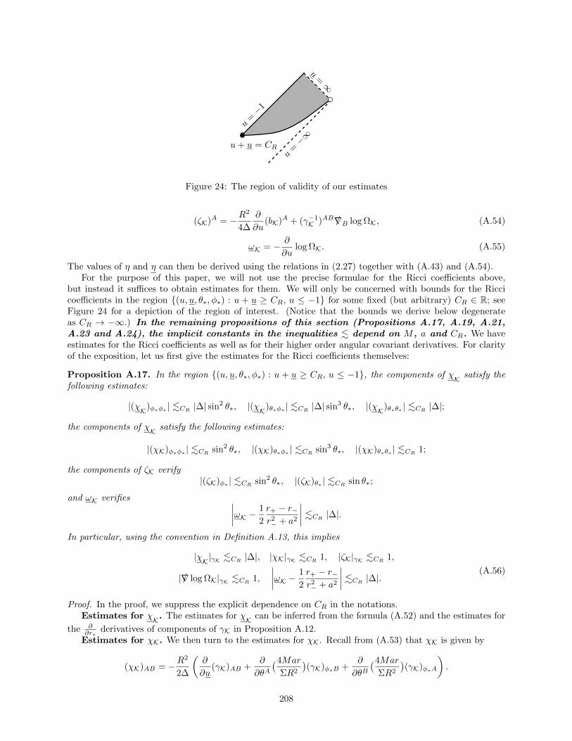
u=∞

u+ u = CRu

=−∞

u=−1

Figure 24: The region of validity of our estimates

(ζK)A = −R2

4∆

∂

∂u(bK)A + (γ−1

K )AB /∇B log ΩK, (A.54)

ωK = − ∂

∂ulog ΩK. (A.55)

The values of η and η can then be derived using the relations in (2.27) together with (A.43) and (A.54).For the purpose of this paper, we will not use the precise formulae for the Ricci coefficients above,

but instead it suffices to obtain estimates for them. We will only be concerned with bounds for the Riccicoefficients in the region (u, u, θ∗, φ∗) : u + u ≥ CR, u ≤ −1 for some fixed (but arbitrary) CR ∈ R; seeFigure 24 for a depiction of the region of interest. (Notice that the bounds we derive below degenerateas CR → −∞.) In the remaining propositions of this section (Propositions A.17, A.19, A.21,A.23 and A.24), the implicit constants in the inequalities . depend on M , a and CR. We haveestimates for the Ricci coefficients as well as for their higher order angular covariant derivatives. For clarityof the exposition, let us first give the estimates for the Ricci coefficients themselves:

Proposition A.17. In the region (u, u, θ∗, φ∗) : u + u ≥ CR, u ≤ −1, the components of χK satisfy thefollowing estimates:

|(χK)φ∗φ∗ | .CR |∆| sin2 θ∗, |(χK)θ∗φ∗ | .CR |∆| sin3 θ∗, |(χK)θ∗θ∗ | .CR |∆|;

the components of χK satisfy the following estimates:

|(χK)φ∗φ∗ | .CR sin2 θ∗, |(χK)θ∗φ∗ | .CR sin3 θ∗, |(χK)θ∗θ∗ | .CR 1;

the components of ζK verify|(ζK)φ∗ | .CR sin2 θ∗, |(ζK)θ∗ | .CR sin θ∗;

and ωK verifies ∣∣∣∣ωK − 1

2

r+ − r−r2− + a2

∣∣∣∣ .CR |∆|.In particular, using the convention in Definition A.13, this implies

|χK|γK .CR |∆|, |χK|γK .CR 1, |ζK|γK .CR 1,

| /∇ log ΩK|γK .CR 1,

∣∣∣∣ωK − 1

2

r+ − r−r2− + a2

∣∣∣∣ .CR |∆|. (A.56)

Proof. In the proof, we suppress the explicit dependence on CR in the notations.Estimates for χK. The estimates for χK can be inferred from the formula (A.52) and the estimates for

the ∂∂r∗

derivatives of components of γK in Proposition A.12.Estimates for χK. We then turn to the estimates for χK. Recall from (A.53) that χK is given by

(χK)AB = −R2

2∆

(∂

∂u(γK)AB +

∂

∂θA(4Mar

ΣR2

)(γK)φ∗B +

∂

∂θB(4Mar

ΣR2

)(γK)φ∗A

).

208

The term −R2

2∆∂∂u (γK)AB can be dealt with using the estimates for the ∂

∂r∗derivatives of components of γK

in Proposition A.12 (in a similar manner as the estimates for χK, except for an extra factor of R2

2∆ ).

For the term ∂∂θA

(4MarΣR2

)(γK)φ∗B , notice that this is only non-vanishing when θA = θ∗. Therefore, using

(A.45), we have ∣∣∣∣ ∂∂u (γK)θ∗θ∗ + 2∂

∂θ∗

(4Mar

ΣR2

)(γK)φ∗θ∗

∣∣∣∣ . |∆|,∣∣∣∣ ∂∂u (γK)θ∗φ∗ +∂

∂θ∗

(4Mar

ΣR2

)(γK)φ∗φ∗

∣∣∣∣ . |∆| sin3 θ,∣∣∣∣ ∂∂u (γK)φ∗φ∗

∣∣∣∣ . |∆| sin2 θ,

from which the desired bounds for χK follow.Estimates for ζK. We next estimate ζK. We first control ζφ∗ and ζθ∗ . By (A.54), we need to control

−R2

4∆∂∂u (bK)A = −R2

4∆∂∂r∗

(bK)A and (γ−1K )AB /∇B log ΩK. For the first term, by (A.43) we only have the

φ∗-component, which satisfies the bound∣∣∣∣R2

4∆

∂

∂r∗(bK)φ∗

∣∣∣∣ =

∣∣∣∣R2

4∆

(∂

∂r∗

4Mar

ΣR2

)∣∣∣∣ . 1

thanks to the estimates in Proposition A.5. For the second term, differentiating the expression of ΩK in(A.43), using the expression of γ−1

K in (A.44) and applying the estimates in Proposition A.5, we obtain

|(γ−1K )θ∗θ∗ /∇θ∗ log ΩK| . sin θ∗, |(γ−1

K )φ∗θ∗ /∇θ∗ log ΩK| . sin θ∗.

Combining the above observations yields |ζφ∗ | . 1 and |ζθ∗ | . sin θ∗, which in turn gives the desired estimatesfor indices down after using the properties of γK in (A.43).

Estimates for ωK. To derive the estimates for ωK, recall from Proposition 2.4 that

ωK = − ∂

∂ulog ΩK = − ∂

∂r∗log ΩK,

where the last equality holds due since log ΩK is independent of t. The desired estimate then follows thanksto (A.49).

Estimates for the Ricci coefficients with respect to the γK norm. Finally, to obtain (A.56),observe that by (A.44), we have

|(γ−1K )φ∗φ∗ | . 1

sin2 θ∗, |(γ−1

K )θ∗θ∗ |+ |(γ−1K )θ∗φ∗ | . 1.

The conclusion then follows from the previous bounds together with the estimates in Proposition A.16.

Remark A.18. Note that on the Cauchy horizon CH+, we have ωK = 12r+−r−r2−+a2 > 0. The positivity of ωK in

a neighbourhood of the Cauchy horizon is the origin of the local blue shift effect, which plays an importantrole in the present work.

We also have the following bounds for the higher derivatives of the Ricci coefficients:

Proposition A.19. Using the convention introduced in Definition A.13, for every I ∈ N, the followingbounds hold for the angular covariant derivatives of the Ricci coefficients on Kerr spacetime in the region(u, u, θ∗, φ∗) : u+ u ≥ CR, u ≤ −1:∑

0≤i≤I

|( /∇K)iχK|γK .CR,I |∆|,∑

0≤i≤I

(|( /∇K)iχK|γK + |( /∇K)iζK|γK + |( /∇K)i+1 log ΩK|γK) .CR,I 1,

∑1≤i≤I

|( /∇K)iωK|γK .CR,I |∆|.

Here, the implicit constants depend on CR and I, in addition to M and a.

209

Remark A.20. We emphasise that the bounds for /∇iKωK hold only when i ≥ 1. For i = 0, we instead havethe bound in Proposition A.17, so that ωK is a non-zero constant at the Cauchy horizon.

The Gauss curvature of the spheres Su,u can be bounded as follows:

Proposition A.21. For every I ∈ N, the following bound holds for the angular covariant derivative of theGauss curvature of the 2-spheres Su,u: ∑

0≤i≤I

supu,u|( /∇K)iKK|γK .I 1,

where the implicit constant depends on I, in addition to M and a.

Proof. According to (A.43) and the estimates in Propositions A.5 and A.6, for every u and u, the metric γKis smooth. Moreover, γK also has a smooth limit as u+ u→ ±∞. Since for every i ∈ N ∪ 0, ( /∇K)iKK isintrinsic to the 2-spheres Su,u, i.e. it only depends on γK and its tangential derivatives along the 2-spheres,we obtain the desired estimate.

In the next proposition, we will obtain a uniform upper bound on the isoperimetric constant on Su,u.Before we proceed, we recall the definition of the isoperimetric constant. Given a Riemannian 2-surface(S, γ), we define the isoperimetric constant I(S, γ) by

I(S, γ) = supU

∂U∈C1

minArea(U),Area(U c)(Perimeter(∂U))2

.

The importance of the isoperimetric constant in the context of this paper lies in the fact that it is intimatelytied to the constants in the Sobolev embedding theorems, c.f. Propositions 5.1, 5.2, 5.4, 5.5. We now statethe bound we have for the isoperimetric constant on the Kerr spacetime:

Proposition A.22. There exists a constant IK > 0 (depending on M and a) such that

supu,u

I(Su,u, γK) ≤ IK.

Proof. First, notice that given two 2-spheres Su1,u1and Su2,u2

such that u1+u1 = u2+u2 = r∗, by identifyingthe value of the coordinate functions θ∗ and φ∗ on Su1,u1

and Su2,u2, it is easy to see that Su1,u1

and Su2,u2

are in fact isometric. In particular, the isoperimetric constant is only a function of the r∗ value associatedto the 2-sphere. Second, since the isoperimetric constant is continuous in r∗, it is uniformly bounded forr∗ ∈ K, where K is any fixed compact set of R. It therefore suffices to show that I(Su,u, γK) does not go toinfinity as r∗ → ±∞, which is obvious since γK has a smooth limit as r∗ →∞ or r∗ → −∞.

A.7 Estimates for the null curvature components on Kerr spacetime

Since the Kerr metric is a solution to the Einstein vacuum equations (1.1), after using (3.5) in Section 3.1,Propositions A.17 and A.19 imply estimates for the renormalised null curvature components βK, σK andβK. These can be obtained after writing the Einstein vacuum equations in the double null coordinate gauge.More precisely, in the region (u, u, θ∗, φ∗) : u+u ≥ CR, u ≤ −1 for CR ∈ R, we have the following bounds:

Proposition A.23. Using the convention introduced in Definition A.13, for every CR ∈ R and I ∈ N,the angular covariant derivatives of the null curvature components on Kerr spacetime satisfy the followingestimates in the region (u, u, θ∗, φ∗) : u+ u ≥ CR, u ≤ −1:∑

0≤i≤I

|( /∇K)iβK|γK .CR,I |∆|,∑

0≤i≤I

|( /∇K)iσK|γK .CR,I 1,∑

0≤i≤I

|( /∇K)iβK|γK .CR,I 1.

Here, the implicit constants depend on CR and I, in addition to M and a.

Proof. This is a direct consequence of the fact that the Kerr metric is a solution to the Einstein vacuumequations and the application of the constraint equations (3.5).

210

Combining the estimates in Propositions A.19, A.21 and A.23, we also immediately infer the followingbounds for µK, µK and ω/K (cf. (2.26)):

Proposition A.24. Using the convention introduced in Definition A.13, for every CR ∈ R and I ∈ N, thefollowing estimates hold in the region (u, u, θ∗, φ∗) : u+ u ≥ CR, u ≤ −1:∑

0≤i≤I

|( /∇K)iµK|γK .CR,I 1,∑

0≤i≤I

|( /∇K)iµK|γK .CR,I 1,∑

0≤i≤I

|( /∇K)iω/K|γK .CR,I |∆|.

Here, the implicit constants depend on CR and I, in addition to M and a.

A.8 Spacelike hypersurfaces in MKerr

In Theorem 1, the initial data are posed on a spacelike hypersurface. In order to compare the initial datawith that of Kerr, we briefly discuss in this subsection the induced metric and second fundamental form onspacelike hypersurfaces in MKerr. We will moreover do so in a coordinate system that is easy to comparewith the double null coordinate system that we discussed earlier.

More precisely, we consider a smooth embedded spacelike hypersurface (with boundary)150 ΣK ⊂MKerr

given byΣK = (u, u) : u+ u = CR, u ≥ 1 × S2,

where CR ∈ R is a constant (but otherwise arbitrary), u and u are the null coordinates defined in Section A.4and S2 corresponds to 2-spheres of constant u, u values.

Let (θ1, θ2) be an arbitrary local coordinates system on S2 satisfying LθA = 0. (For instance (θ1 =θ∗, θ

2 = φ∗) is one such system of local coordinates.) Introducing the functions τ.= u, θAΣ

.= θA for A = 1, 2,

it is easy to see that (τ, θ1Σ, θ

2Σ) forms a system of local coordinates on ΣK. In this coordinate system, the

induced metric gK on ΣK is given by

gK = ΦKdτ ⊗ dτ + (wK)A(dτ ⊗ dθAΣ + dθAΣ ⊗ dτ) + (γK)ABdθAΣ ⊗ dθBΣ , (A.57)

whereΦK = (γK)AB(bK)A(bK)B + 4Ω2

K, (wK)A = −(γK)AB(bK)B

and (γK)AB and (bK)A are as in (A.43).Notice that151

∂

∂τ= − ∂

∂u+

∂

∂u,

∂

∂θ1Σ

=∂

∂θ1,

∂

∂θ2Σ

=∂

∂θ2

forms a local basis of the tangent space of ΣK.

Next, we claim that the vector field

NK =1

2ΩK

(∂

∂u+

∂

∂u+ bBK

∂

∂θB

)=

1

2ΩK

(e3 + Ω2

Ke4

)is the future-directed unit normal to ΣK. To see this, we first check that it is orthogonal to the tangentvectors of ΣK, i.e.

gK

(NK,

∂

∂θA

)= 0, gK

(NK,−

∂

∂u+

∂

∂u

)=

1

2ΩKgK(e3 + Ω2

Ke4,−e3 + Ω2Ke4) = 0.

We then compute the norm of NK:

gK(NK, NK) =1

4Ω2K

2Ω2Kg(e3, e4) = −1.

150In this subsection, ΣK is used to denote the spacelike hypersurface defined below. This is not to be confused with the Σ in(A.1).151Here, we have used the convention that ∂

∂τ, ∂∂θ1Σ

and ∂∂θ2Σ

are coordinate vector fields in the (τ, θ1Σ, θ

2Σ)-coordinate system

on ΣK.

211

Therefore, NK is indeed the future-directed unit normal to ΣK. In particular, this also shows that ΣK is aspacelike hypersurface.

On the other hand, define nK by

nK =1

2ΩK

(∂

∂τ− (γ−1)AB(wK)A

∂

∂θBΣ

)=

1

2ΩK

(− ∂

∂u+

∂

∂u+ bBK

∂

∂θB

),

which, by a similar computation as above, is tangent to ΣK and is normal (with respect to the inducedRiemannian metric on ΣK) to the 2-spheres given by constant-τ . By the formulae for NK and nK, we obtain

LK =∂

∂u= ΩK(NK − nK) (A.58)

and

LK =∂

∂u+ (bK)A

∂

∂θA= ΩK(NK + nK). (A.59)

Here, LK and LK are the vector fields L and L defined in (A.51), where we have used the subscript K toemphasise that its definition depends on the Kerr metric.

References

[1] S. Alexakis, A. D. Ionescu, and S. Klainerman. Uniqueness of smooth stationary black holes in vacuum:small perturbations of the Kerr spaces. Commun. Math. Phys., 299:89–127, 2010.

[2] Y. Angelopoulos, S. Aretakis, and D. Gajic. Late-time asymptotics for the wave equation on sphericallysymmetric, stationary spacetimes. arXiv:1612.01566, preprint, 2016.

[3] S. Aretakis. Horizon instability of extremal black holes. Adv. Theor. Math. Phys., 19(3):507–530, 2015.

[4] S. Bhattacharjee, S. Sarkar, and A. Virmani. Internal structure of charged AdS black holes. Phys.Rev. D, 93(12):124029, 2016.

[5] P. Bizon and A. Rostworowski. Weakly turbulent instability of anti–de Sitter spacetime. Phys. Rev.Lett., 107(3):031102, 2011.

[6] A. Bonanno, S. Droz, W. Israel, and S. M. Morsink. Structure of the charged spherical black holeinterior. Proc. R. Soc. Lond. A, 450:553–567, 1995.

[7] R. H. Boyer and R. W. Lindquist. Maximal analytic extension of the Kerr metric. J. Math. Phys.,8(2):265–281, 1967.

[8] P. R. Brady and C. M. Chambers. Nonlinear instability of Kerr-type Cauchy horizons. Phys. Rev. D,51(8):4177, 1995.

[9] P. R. Brady, I. G. Moss, and R. C. Myers. Cosmic censorship: as strong as ever. Phys. Rev. Lett.,80(16):3432, 1998.

[10] P. R. Brady and J. D. Smith. Black hole singularities: a numerical approach. Phys. Rev. Lett.,75(7):1256–1259, 1995.

[11] L. M. Burko. Structure of the black holes Cauchy-horizon singularity. Phys. Rev. Lett., 79(25):4958–4961, 1997.

[12] B. Carter. Global structure of the Kerr family of gravitational fields. Phys. Rev., 174(5):1559, 1968.

[13] B. Carter. Axisymmetric black hole has only two degrees of freedom. Phys. Rev. Lett., 26(6):331, 1971.

[14] B. Carter. Black hole equilibrium states. In C. DeWitt and B. S. DeWitt, editors, Black holes/Lesastres occlus (Ecole d’Ete Phys. Theor., Les Houches, 1972), pages 57–214. Gordon and Breach, NewYork, 1973.

212

[15] Y. Choquet-Bruhat and R. P. Geroch. Global aspects of the Cauchy problem in general relativity.Commun. Math. Phys., 14:329–335, 1969.

[16] D. Christodoulou. Bounded variation solutions of the spherically symmetric Einstein-scalar field equa-tions. Comm. Pure Appl. Math., 46(8):1131–1220, 1993.

[17] D. Christodoulou. Examples of naked singularity formation in the gravitational collapse of a scalarfield. Ann. of Math. (2), 140(3):607–653, 1994.

[18] D. Christodoulou. On the global initial value problem and the issue of singularities. Class. QuantumGrav., 16:A23–A35, 1999.

[19] D. Christodoulou. The instability of naked singularities in the gravitational collapse of a scalar field.Ann. of Math., 149:183–217, 1999.

[20] D. Christodoulou. The formation of black holes in general relativity. EMS Monographs in Mathematics.European Mathematical Society (EMS), Zurich, 2009.

[21] D. Christodoulou and S. Klainerman. The global nonlinear stability of the Minkowski space, volume 41of Princeton Mathematical Series. Princeton University Press, Princeton, NJ, 1993.

[22] D. Civin. Stability of charged rotating black holes for linear scalar perturbations. PhD thesis, Universityof Cambridge, 2014.

[23] J. L. Costa, P. M. Girao, J. Natario, and J. D. Silva. On the global uniqueness for the Einstein–Maxwell–scalar field system with a cosmological constant. Commun. Math. Phys., 339(3):903–947,2015.

[24] J. L. Costa, P. M. Girao, J. Natario, and J. D. Silva. On the global uniqueness for the Einstein–Maxwell–scalar field system with a cosmological constant: Part 3. Mass inflation and extendibility ofthe solutions. Annals of PDE, 3(1):8, Mar 2017.

[25] J. L. Costa, P. M. Girao, J. Natario, and J. D. Silva. On the occurrence of mass inflation for theEinstein–Maxwell–scalar field system with a cosmological constant and an exponential Price law.arXiv:1707.08975, preprint, 2017.

[26] M. Dafermos. Stability and instability of the Cauchy horizon for the spherically symmetric Einstein-Maxwell-scalar field equations. Ann. of Math. (2), 158(3):875–928, 2003.

[27] M. Dafermos. The interior of charged black holes and the problem of uniqueness in general relativity.Comm. Pure Appl. Math., 58(4):445–504, 2005.

[28] M. Dafermos. Spherically symmetric spacetimes with a trapped surface. Class. Quantum Grav.,22(11):2221–2232, 2005.

[29] M. Dafermos. Black holes without spacelike singularities. Commun. Math. Phys., 332(2):729–757,2014.

[30] M. Dafermos and G. Holzegel. Dynamic instability of solitons in 4 + 1-dimensional gravity withnegative cosmological constant. https://www.dpmms.cam.ac.uk/˜md384/ADSinstability.pdf, 2006.

[31] M. Dafermos, G. Holzegel, and I. Rodnianski. A scattering theory construction of dynamical vacuumblack holes. arXiv:1306.5364, preprint, to appear in J. Diff. Geom., 2013.

[32] M. Dafermos and J. Luk. The interior of dynamical vacuum black holes II: event horizon data and thestability of the red-shift region. in preparation, 2017.

[33] M. Dafermos and J. Luk. The interior of dynamical vacuum black holes III: The C0-stability of thebifurcation sphere of the Kerr Cauchy horizon. in preparation, 2017.

213

[34] M. Dafermos and J. Luk. The stability and instability properties of Cauchy horizons and the strongcosmic censorship conjecture. preprint, 2017.

[35] M. Dafermos and I. Rodnianski. A proof of Price’s law for the collapse of self-gravitating scalar field.Invent. Math., 162:381–457, 2005.

[36] M. Dafermos, I. Rodnianski, and Y. Shlapentokh-Rothman. Decay for solutions of the wave equationon Kerr exterior spacetimes III: The full subextremal case |a| < M . Ann. of Math. (2), 183(3):787–913,2016.

[37] M. Dafermos, I. Rodnianski, and Y. Shlapentokh-Rothman. A scattering theory for the wave equationon Kerr black hole exteriors. arXiv:1412.8379, to appear in Ann. Sci. Ecole Norm. S., 2017.

[38] M. Dafermos and Y. Shlapentokh-Rothman. Time-translation invariance of scattering maps and blue-shift instabilities on Kerr black hole spacetimes. Commun. Math. Phys., 350(3):985–1016, 2017.

[39] W. de Sitter. Einstein’s theory of gravitation and its astronomical consequences. Third paper. Mon.Notices Royal Astron. Soc., 78:3–28, 1917.

[40] O. J. Dias, G. T. Horowitz, D. Marolf, and J. E. Santos. On the nonlinear stability of asymptoticallyanti-de sitter solutions. Class. Quantum Grav., 29(23):235019, 2012.

[41] J. Earman. Bangs, crunches, whimpers, and shrieks: Singularities and acausalities in relativisticspacetimes. Oxford University Press, 1995.

[42] A. Einstein. Die Feldgleichungen der Gravitation. Sitzungsber. K. Preuss. Akad. Wiss, pages 844–847,1915.

[43] A. Einstein. Kosmologische Betrachtungen zur allgemeinen Relativitatstheorie. Sitzungsber. K. Preuss.Akad. Wiss, pages 142–152, 1917.

[44] A. T. Franzen. Boundedness of massless scalar waves on Reissner-Nordstrom interior backgrounds.Commun. Math. Phys., 343(2):601–650, 2016.

[45] A. T. Franzen. Boundedness of massless scalar waves on Kerr interior backgrounds. preprint, 2017.

[46] H. Friedrich. On the existence of n-geodesically complete or future complete solutions of Einstein’sfield equations with smooth asymptotic structure. Commun. Math. Phys., 107(4):587–609, 1986.

[47] H. Friedrich. Einstein equations and conformal structure: existence of anti-de Sitter-type space-times.J. Geom. Phys., 17(2):125–184, 1995.

[48] D. Gajic. Linear waves in the interior of extremal black holes I. Commun. Math. Phys., 353(2):717–770,2017.

[49] D. Gajic. Linear waves in the interior of extremal black holes II. arXiv:1512.08953, to appear in Ann.Henri Poincare, 2017.

[50] R. Geroch and G. T. Horowitz. Global structure of spacetimes. In S. W. Hawking and W. Israel, editors,General Relativity: An Einstein centenary survey, pages 212–293. Cambridge University Press, 1979.

[51] R. Geroch and G. T. Horowitz. Asymptotically simple does not imply asymptotically Minkowskian.Phys. Rev. Lett., 40:203–206, 1978.

[52] R. Geroch, E. H. Kronheimer, and R. Penrose. Ideal points in space-time. Proc. Roy. Soc. A,327(1571):545–567, 1972.

[53] G. W. Gibbons. Anti-de-Sitter spacetime and its uses. In G. W. Gibbons and S. Cotsakis, editors,Mathematical and quantum aspects of relativity and cosmology. Proceedings, 2nd Samos Meeting oncosmology, geometry and relativity, Pythagoreon, Samos, Greece, August 31-September 4, 1998, volume537 of Lecture notes in Physics, pages 102–142. Springer, 2011.

214

[54] E. Gleeson. Linear Instability of the Reissner-Nordstrom Cauchy Horizon. Master’s thesis, Universityof Cambridge, arXiv:1701.06668, 2017.

[55] M. L. Gnedin and N. Y. Gnedin. Destruction of the Cauchy horizon in the Reissner-Nordstrom blackhole. Class. Quantum Grav., 10(6):1083, 1993.

[56] N. Y. Gnedin and M. Gnedina. Instability of the internal structure of a Reissner-Nordstrom black-hole.Soviet Astronomy, 36:296, 1992.

[57] S. W. Hawking. The occurrence of singularities in cosmology. III. Causality and singularities. Proc.Roy. Soc. A., 300(1461):187–201, 1967.

[58] S. W. Hawking and G. F. R. Ellis. The large scale structure of space-time. Cambridge Monographs onMathematical Physics. Cambridge University Press, Cambridge, 1973.

[59] S. W. Hawking and R. Penrose. The singularities of gravitational collapse and cosmology. Proc. Roy.Soc. A, 314(1519):529–548, 1970.

[60] E. Hebey. Nonlinear analysis on manifolds: Sobolev spaces and inequalities, volume 5 of CourantLecture Notes in Mathematics. New York University, Courant Institute of Mathematical Sciences, NewYork; American Mathematical Society, Providence, RI, 1999.

[61] P. Hintz. Non-linear stability of the Kerr-Newman-de Sitter family of charged black holes.arXiv:1612.04489, preprint, 2016.

[62] P. Hintz. Boundedness and decay of scalar waves at the Cauchy horizon of the Kerr spacetime.arXiv:1512.08003, to appear in Comment. Math. Helv., 2017.

[63] P. Hintz and A. Vasy. The global non-linear stability of the Kerr-de Sitter family of black holes.arXiv:1606.04014, preprint, 2016.

[64] W. A. Hiscock. Evolution of the interior of a charged black hole. Phys. Rev. Lett., 83A:110–112, 1981.

[65] G. Holzegel, J. Luk, J. Smulevici, and C. Warnick. Asymptotic properties of linear field equations inanti-de Sitter space. arXiv:1502.04965, preprint, 2015.

[66] G. Holzegel and J. Smulevici. Decay properties of Klein-Gordon fields on Kerr-AdS spacetimes. Comm.Pure and Appl. Math., 66(11):1751–1802, 2013.

[67] G. Holzegel and J. Smulevici. Quasimodes and a lower bound on the uniform energy decay rate forKerr-AdS spacetimes. Anal. PDE, 7(5):1057–1090, 2014.

[68] G. T. Horowitz. Finding a statement of cosmic censorship. Gen. Rel. Gravit., 10(12):1057–1061, 1979.

[69] J. T. Jebsen. Uber die allgemeinen kugelsymmetrischen Losungen der Einsteinschen Gravitationsgle-ichungen im Vakuum. Ark. Mat. Astr. Fys., 15:1–9, 1921.

[70] R. Kerr. Gravitational field of a spinning mass as an example of algebraically special metrics.Phys. Rev. Lett., 11 (5):237–238, 1963.

[71] S. Klainerman, I. Rodnianski, and J. Szeftel. The bounded L2 curvature conjecture. Invent. Math.,202(1):91–216, 2015.

[72] J. Kommemi. The global structure of spherically symmetric charged scalar field spacetimes. Commun.Math. Phys., 323(1):35–106, 2013.

[73] J. Kommemi. The global structure of spherically symmetric charged scalar field spacetimes. PhD thesis,University of Cambridge, Cambridge, 2013.

[74] M. D. Kruskal. Maximal extension of Schwarzschild metric. Phys. Rev. (2), 119:1743–1745, 1960.

215

[75] J. Leray. Hyperbolic differential equations. The Institute for Advanced Study, Princeton, N. J., 1953.

[76] E. M. Lifshitz and I. M. Khalatnikov. Investigations in relativistic cosmology. Adv. Phys., 12(46):185–249, 1963.

[77] R. W. Lindquist and J. A. Wheeler. Dynamics of a lattice universe by the Schwarzschild-cell method.Rev. Mod. Phys., 29:432–443, Jul 1957.

[78] J. Luk. Improved decay for solutions to the linear wave equation on a Schwarzschild black hole. Ann.Henri Poincare, 11(5):805–880, 2010.

[79] J. Luk. On the local existence for the characteristic initial value problem in general relativity. Int.Math. Res. Notices, 2012(12):4625–4678, 2012.

[80] J. Luk. Weak null singularities in general relativity. arXiv:1311.4970, to appear in J. Amer. Math.Soc., https://doi.org/10.1090/jams/888, 2017.

[81] J. Luk and S.-J. Oh. Proof of linear instability of the Reissner–Nordstrom Cauchy horizon under scalarperturbations. Duke Math. J., 166(3):437–493, 2017.

[82] J. Luk and S.-J. Oh. Strong cosmic censorship in spherical symmetry for two-ended asymptoticallyflat initial data I. The interior of the black hole region. arXiv:1702.05715, preprint, 2017.

[83] J. Luk and S.-J. Oh. Strong cosmic censorship in spherical symmetry for two-ended asymptoticallyflat initial data II. The exterior of the black hole region. arXiv:1702.05716, preprint, 2017.

[84] J. Luk and I. Rodnianski. Local propagation of impulsive gravitational waves. Comm. Pure Appl.Math., 68(4):511–624, 2015.

[85] J. Luk and I. Rodnianski. Nonlinear interaction of impulsive gravitational waves for the vacuumEinstein equations. arXiv:1301.1072, to appear in Cambridge J. of Math., 2017.

[86] J. Luk and J. Sbierski. Instability results for the wave equation in the interior of Kerr black holes. J.Funct. Anal., 271(7):1948–1995, 2016.

[87] J. M. McNamara. Behaviour of scalar perturbations of a Reissner–Nordstrom black hole inside theevent horizon. Proc. R. Soc. A., 364:121–134, 1978.

[88] J. M. McNamara. Instability of black hole inner horizons. Proc. Roy. Soc. A, 358(1695):499–517, 1978.

[89] G. Moschidis. A proof of the instability of AdS for the Einstein–null dust system with an inner mirror.arXiv:1704.08681, preprint, 2017.

[90] E. Newman and R. Penrose. An approach to gravitational radiation by a method of spin coefficients.J. Math. Phys., 3(3):566–578, 1962.

[91] B. O’Neill. The geometry of Kerr black holes. A. K. Peters, Ltd., Wellesley, MA, 1995.

[92] J. R. Oppenheimer and H. Snyder. On continued gravitational contraction. Phys. Rev., 56(5):455,1939.

[93] A. Ori. Inner structure of a charged black hole: an exact mass-inflation solution. Phys. Rev. Lett.,67:789–792, 1991.

[94] A. Ori. Perturbative approach to the inner structure of a rotating black hole. Gen. Rel. Gravit.,29(7):881–929, 1997.

[95] A. Ori and E. E. Flanagan. How generic are null spacetime singularities? Phys. Rev. D, 53:1754–1758,1996.

[96] R. Penrose. Structure of Space-Time. In R. Penrose and C. M. DeWitt, editors, Battelle Rencontres,page 222. W. A. Benjamin, New York, 1968.

216

[97] R. Penrose. Gravitational collapse: The role of general relativity. Riv. Nuovo Cim., 1:252–276, 1969.

[98] R. Penrose. Gravitational collapse. In C. Dewitt-Morette, editor, Gravitational Radiation and Gravi-tational Collapse, volume 64 of IAU Symposium, pages 82–91. Springer, 1974.

[99] R. Penrose. Some unsolved problems in classical general relativity. In S.-T. Yau, editor, Seminaron Differential Geometry, volume 102 of Ann. of Math. Stud., pages 631–668. Princeton Univ. Press,Princeton, N.J., 1982.

[100] R. Penrose. Gravitational collapse and space-time singularities. Phys. Rev. Lett., 14:57–59, Jan 1965.

[101] R. Penrose. A remarkable preperty of plane waves in general relativity. Rev. Mod. Phys., 37:215–220,1965.

[102] E. Poisson and W. Israel. Inner-horizon instability and mass inflation in black holes. Phys. Rev. Lett.,63:1663–1666, 1989.

[103] F. Pretorius and W. Israel. Quasispherical light cones of the Kerr geometry. Class. Quantum Grav.,15:2289–2301, 1998.

[104] A. D. Rendall. Reduction of the characteristic initial value problem to the Cauchy problem and itsapplications to the Einstein equations. Proc. Roy. Soc. A, 427(1872):221–239, 1990.

[105] H. Ringstrom. The Cauchy problem in general relativity. ESI Lectures in Mathematics and Physics.European Mathematical Society (EMS), Zurich, 2009.

[106] D. C. Robinson. Uniqueness of the Kerr black hole. Phys. Rev. Lett., 34(14):905, 1975.

[107] I. Rodnianski and J. Speck. Stable Big Bang formation in near-FLRW solutions to the Einstein-scalarfield and Einstein-stiff fluid systems. arXiv:1407.6298, preprint, 2014.

[108] I. Rodnianski and J. Speck. A regime of linear stability for the Einstein-scalar field system withapplications to nonlinear Big Bang formation. arXiv:1407:6293, to appear in Ann. of Math., 2017.

[109] J. Sbierski. Characterisation of the energy of Gaussian beams on Lorentzian manifolds: with applica-tions to black hole spacetimes. Anal. PDE, 8(6):1379–1420, 2015.

[110] J. Sbierski. The C0-inextendibility of the Schwarzschild spacetime and the spacelike diameter inLorentzian geometry. arXiv:1507.00601, to appear in J. Diff. Geom., 2017.

[111] V. Schlue. Decay of the Weyl curvature in expanding black hole cosmologies. arXiv:1610.04172,preprint, 2016.

[112] K. Schwarzschild. Uber das Gravitationsfeld eines Massenpunktes nach der Einsteinschen Theorie.Sitzungsber. K. Preuss. Akad. Wiss, 1:189–196, 1916.

[113] J. L. Synge. The gravitational field of a particle. Proc. Roy. Irish Acad. Sect. A., 53:83–114, 1950.

[114] M. Van de Moortel. Stability and instability of the sub-extremal Reissner-Nordstrom black hole interiorfor the Einstein-Maxwell-Klein-Gordon equations in spherical symmetry. arXiv:1704.05790, preprint,2017.

[115] R. M. Wald. General Relativity. The University of Chicago Press, Chicago, 1984.

217