PHYS 410/555 Computational Physics: Solution of ODEs(Reference Numerical Recipes, Chapters 16, 17)

Overview

• “Theory”

– Casting systems of ODEs in first order form (canonical form)

– Boundary / initial conditions

• Some Basic Numerical Techniques

– Euler method

– Second-order Runge-Kutta

• Using “Canned” Software

– ODEPACK routine lsoda

• Applications

– Quadrature (definite integrals)

– Initial value problems (dynamics)

– Boundary value problems

Note: There are many applications in virtually every sub-field of physics.

Casting Systems of ODEs in First Order Form

• Can always reduce systems of ODEs to set of first order DEs by introducing appropriate new(auxiliary) variables.

Example 1

y′′(x) + q(x)y′(x) = r(x) ′ ≡ d

dx(1)

• Introduce new variable z(x) ≡ y′(x), then (1) becomes

y′ = z (2)

z′ = r − qz (3)

1

Example 2

y′′′′(x) = f(x) (4)

• Introduce new variables

y1(x) ≡ y′(x) (5)

y2(x) ≡ y′′(x) (6)

y3(x) ≡ y′′′(x) (7)

then (4) becomes

y′ = y1 (8)

y′1 = y2 (9)

y′2 = y3 (10)

y′3 = f (11)

• Thus, the generic problem in ODEs is reduced to study of a set of N coupled, first-order DEsfor the functions, yi, i = 1, 2, . . . , N

y′i(x) ≡dyi

dx(x) = fi(x, y1, y2, · · · , yN ) i = 1, 2, . . . N (12)

where the fi(· · ·) are known functions of x and yi

• Equivalent forms: y ≡ (y1, y2, · · · , yN )

y′(x) = f(x,y) (13)

y(t) = f(t,y) (14)

Boundary / Initial Conditions

• ODE problem not completely specified by DEs themselves

• Nature of boundary conditions is crucial aspect of problem

• Generally, BCs are algebraic conditions on certain values of the yi in (12) that are to besatisfied at discrete specified points.

• Generally will need N conditions for N -th order system

• BCs divide ODE problems into 2 broad classes

2

1) Initial Value Problems

• All the yi are given at some starting (initial) value, tmin and we wish to find the yi at somefinal value, tmax, or at some set of values

tn, tmin ≤ tn ≤ tmax n = 0, 1, 2, · · · (15)

2) (Two-point) Boundary Value Problems

• BCs are specified at more than one value of x. Typically some will be specified at x = xmin,the remainder at x = xmax.

• Have already considered some 2-pt BVPs, and their solution via finite difference techniques

We will focus on general techniques / software for solving IVPs, and some simple BVPs.

Some Basic Numerical Techniques for IVPs

We adopt the notation of Numerical Recipes, and illustrate the methods for the case of a scalarequation. The generalization to systems is straightforward.

1) The Euler Method

• Consider two values of x, xn and xn+1 = xn +h (h is often called the “step size”, and is com-pletely analogous to the mesh spacing, h, used in our previous work on FD approximations)

• Then the (forward) Euler method is given by

yn+1 = yn + hf(xn, yn) (16)

• Note that we use this formula to “advance” solution from x = xn to x = xn+1 = xn + h

• Can easily derive from O(h) (forward) finite difference approximation

yn+1 − yn

h= y′n +O(h) (17)

y′ = f(x, y) −→ yn+1 − yn

h= f(xn, yn) (18)

• Accuracy: O(h2) per step. For fixed final x = xf , number of steps scales as h−1, so globalaccuracy is O(h)

• OK for demonstration purposes, but should never be used in practice—not very accurate,not very stable!

3

2) Second-order Runge-Kutta (Mid-point Method)

• The second-order Runge-Kutta method is given by

k1 = hf(xn, yn) (19)

k2 = hf

(

xn +1

2h, yn +

1

2k1

)

(20)

yn+1 = yn + k2 (21)

• Global accuracy: O(h2)

• Derivation

yn+1 − yn

h= f(xn+1/2, yn+1/2) +O(h2) (22)

where xn+1/2 ≡ xn + h/2, yn+1/2 ≡ y(xn+1/2). (Exercise: Verify the above, and compute theactual form of the leading order error term.)

To retain O(h2) accuracy, need to evaluate f(xn+1/2, yn+1/2) to O(h2) (i.e. can neglect O(h2)terms), so, in turn, need to know yn+1/2 to O(h2); proceed via Taylor series expansion

yn+1/2 = yn +1

2hy′n +O(h2)

= yn +1

2k1 +O(h2)

=⇒ yn+1 = yn + hf

(

xn +1

2h, yn +

1

2k1

)

as advertised.

Although it is “good for you” to understand some of the theory that underlies a modern ODEsolver, the state of such solvers is very high, and, as with linear system solvers, can frequently beused as “black boxes”—with the important proviso that we always make every reasonable attemptto validate our results (convergence tests, independent residual tests, conserved quantities, etc.)

4

ODEPACK

• Public-domain collection of routines for solution of systems of ODEs (IVPs)

• We will focus on one routine, lsoda, which has the following header:

subroutine lsoda(f, neq, y, t, tout, itol, rtol, atol, itask,

& istate, iopt, rwork, lrw, iwork, liw, jac, jt)

external f, jac

integer neq, itol, itask, istate, iopt, lrw, liw, jt

real*8 t, tout, rtol, atol

real*8 y(neq), rwork(lrw)

integer iwork(liw)

See source code and sample “driver” program (tlsoda.f) for full description of parametersand routine operation

• f, jac: Names of routines (subroutines) for evaluating right hand side of ODES (f), andJacobian of system (jac). f is required, jac is optional, typically a “dummy” routine

• neq: number of equations / size of system (canonical first-order form)

• y: On input, (approximate) values of unknowns at t = t ( y(i) , i = 1 , neq ); Onoutput, (approximate) values of unknowns at t = tout

• t, tout: Limits of current integration interval

• itol, rtol, atol: Tolerance (error-control) parameters (see lsoda.f, tlsoda.f for details)

• itask: Set = 1 for normal operation

• istate: Set = 1 intially for normal operation, thereafter set = 2 for normal operation (routinewill automatically do this if integration on first interval is successful); check for negative valueon return to detect abnormal completion

• iopt: Normally set = 0 (no optional inputs, but, again, refer to the source code for fulldetails)

• rwork(lrw): real*8 work array of length lrw;minimum value of lrw is 22 + 16 * neq

• iwork(liw): integer work array of length liw;minimum value of liw is 20 + neq

• jt: Set = 2 for normal operation—supply “dummy” Jacobian routine, lsoda will approxi-mately compute Jacobian numerically if and when necessary

Crucial User-supplied Routine Called by lsoda

• f: Evaluates ”RHS” of system of ODEs (12); must have header as follows

5

subroutine f(neq, t, y, ydot)

implicit none

integer neq

real*8 t, y(neq), ydot(neq)

• Inputs: neq, t, ( y(j) , j = 1 , neq )

• Output: ( ydot(j) , j = 1 , neq )

lsoda Tolerance Parameters: itol, atol, rtol

• lsoda will control step-size, order of method and type of method so that estimated local errorin y(i) is less than

ewt(i) = rtol * abs(y(i)) + atol itol .eq. 1

ewt(i) = rtol * abs(y(i)) + atol(i) itol .eq. 2

Thus, local error tests passes if, for each component y(i), either the absolute error is lessthan atol (or atol(i)), or the relative error is less than rtol

Choosing Error Tolerances

• Can experiment, but rtol = atol = tol (single control parameter) often works well, par-ticularly for yi that exhibit significant dynamical range

• Some exceptions (of course); for example, consider 2-d motion in polar coordinates, (r, θ). Ifwe use relative control, then for θ ≫ 2π, “acceptable local error” δθ will increase. Better ideato try to keep δθ constant via “pure absolute” control (rtol = 0.0d0)

• Solution eror will almost certainly grow with time, so for fixed final integration time, tf , willneed to calibrate error estimates, i.e. assume that

∥

∥

∥ycomputed(tf ) − yexact(tf )∥

∥

∥ ≈ κ(tf )tol (23)

where κ(tf ) can be determined via calibration if yexact is known

• However, even if yexact is not known (typical case!), (23) tells us that we can expect error(at fixed time) to be proportional to tol; e.g. if tol goes from 1.0d-6 -> 1.0d-10, shouldexpect solution error to be down by about 4 orders of magnitude

• Caveat emptor! (“User beware!”)

Checking/validating Results From ODE Integrators

1) Monitoring Conserved Quantities

• Example: For dynamical systems with a Lagrangian (Hamiltonian), total energy, E(t) isconserved: dE/dt = 0

• Monitor variation δE(t, ǫ) of computed energy E(t, ǫ):

δE(t, ǫ) = E(t, ǫ) − E(tmin, ǫ) (24)

6

where ǫ is the error tolerance for the integrator.

• Should find that this is an O(ǫ) quantity, i.e. for ǫ sufficiently small, should have

δE(t, ǫ) = ǫf(t) + higher order terms (25)

• Thus, e.g., if we take ǫ → ǫ/10, should see δE → δE/10 (approximately, so long as ǫ ≫ǫmachine)

2) Independent Residual Evaluation

• Idea: Attempt to directly verify that approximate solution, u (u previously y!) satisfies theODE(s) through the use of an independent discretization of the ODE (i.e. a discretizationdistinct from that used by the ODE integrator).

• Note: In numerical analysis, a residual quantity is one that should tend to 0 in some appro-priate limit

• Let

L [u(t)] ≡ Lu(t) = 0 (26)

be our ODE, where L is a differential operator, and u, in general can be a vector of functions;will assume that L is linear, but technique generalizes to non-linear case

• Let u(t, ǫ) be the solution computed by our ODE integrator for tolerance ǫ, and considercomputing u on a regular mesh of output times

th ≡ tn = tmin, tmin + h, tmin + 2h, · · · (27)

and consider, for concreteness, a second-order (in h) finite difference approximation to theODE

Lhuh = 0 Lh = L+O(h2) (28)

• Note that (28) defines uh, and that

uh(t) 6= u(

th, ǫ)

(29)

• The finite difference operator Lh can be expanded as follows

Lh = L+ h2E2 + h4E4 + · · · (30)

where, as discussed previously, E2, E4, etc. are higher order differential operators (involvehigher order derivatives than L).

• Now, we can write

u(t, ǫ) = u(t) + e(t, ǫ) (31)

where e(t, ǫ) is the error in the solution computed using the ODE integrator

• Next, consider the action of Lh on u(t, ǫ); suppressing explicit t-dependence, we have

7

Lhu(ǫ) =(

L+ h2E2 + h4E4 + · · ·)

(u+ e(ǫ)) (32)

= Lu+ h2E2u+ · · · + Lhe(ǫ) (33)

≈ h2E2 [u] + Lh [e(ǫ)] (34)

• Now, assume that

h2E2 [u] ≫ Lh [e(ǫ)] (35)

then

Lhu ≈ h2E2 [u] = O(h2) (36)

• With a high-accuracy ODE solver such as lsoda, it is usually possible to satisfy (35), at leastover some time interval (tmin, tmax), and as long as h is not chosen too small

• Note: Key idea is to show/check correctness of implementation; e.g. checking for errors incoding of equations.

8

Example:

• Consider the ODE describing simple harmonic motion, (with the gross abuse of notation,′ ≡ d/dt!):

u′′(t) = −u(t) (37)

that we will solve on 0 ≤ t ≤ tmax with the initial values u(0) and u′(0) given

• General solution of (37) is

u(t) = A sin(t) +B cos(t) (38)

u′(t) = A cos(t) −B sin(t) (39)

Evaluating (39) at t = 0 yields

A = u′(0) (40)

B = u(0) (41)

So specific solution satisfying initial conditions is

u(t) = u′(0) sin(t) + u(0) cos(t) (42)

• Cast (37) in canonical form; define

y1 ≡ u (43)

y2 ≡ u′ (44)

Then (37) becomes

y′1 ≡ y2 (45)

y′2 ≡ −y1 (46)

9

• RHS routine called by lsoda

c===========================================================

c Implements differential equations:

c

c u’’ = -u

c

c y(1) := u

c y(2) := u’

c

c y(1)’ := y(2)

c y(2)’ := -y(1)

c

c Called by ODEPACK routine LSODA.

c===========================================================

subroutine fcn(neq,t,y,yprime)

implicit none

integer neq

real*8 t, y(neq), yprime(neq)

yprime(1) = y(2)

yprime(2) = -y(1)

return

end

Independent Residual Evaluator

• First, rewrite (37) in form (26)

u′′(t) + u(t) = 0 (47)

• Next, using e.g. lsoda, generate solution u(th, ǫ) on a level-ℓ uniform mesh:

thn = 0, h, 2h, · · · tmax (48)

with

h =tmax

2ℓ(49)

• Then, apply O(h2) finite-difference discretization of (47) to u to compute residual Rn:

Rn ≡ un+1 − 2un + un−1

h2+ un n = 1, 2, · · · 2ℓ − 1 (50)

10

• In particular, should find that RMS value (ℓ2 norm) of Rn is an O(h2) quantity:

[

∑

n |Rn|22ℓ − 1

]1

2

≡ ‖R‖2 = O(h2) (51)

See tlsoda.f, chk-tlsoda.f for implementation.

Note on Solution Sensitivity/Ill-conditioning

• In integrating from t to tout, lsoda will typically evaluate RHS of ODEs at many intermediatevalues tI , t ≤ tI ≤ tout according to the details of the algorithm, and the user-specifiedtolerances; these tI are typically “invisible” to the user

• If, as is frequently the case, one wants to tabulate the solution at many values, e.g. on a grid

tn ≡ tmin, tmin + h, · · · tmax − h, tmax (52)

then will generally find that, for fixed tolerance, the computed value at t = tmax, e.g., willdepend on specifics of the output values of tn requested

• If results are highly dependent on choice of tn, this is a sign that problem is sensitive (poorlyconditioned); the gravitational n-body problem is a classic example

• In such a case, will also tend to find significant dependence of results on small changes inerror tolerances

BOTTOM LINE: Need to be CAREFUL in use of “black box” software!

IVP Applications

1) “Quadrature”/Definite integrals

• Suppose we wish to evaluate definite integral

∫ x2

x1

f(x)dx (53)

• Consider I(x) such that

dI

dx= f(x) (54)

Then, we have

∫ x2

x1

dI

dxdx =

∫ x2

x1

f(x)dx (55)

=⇒ I(x2) − I(x1) =

∫ x2

x1

f(x)dx (56)

So, with the initial condition

I(x1) = 0 (57)

we have

11

I(x2) =

∫ x2

x1

f(x)dx (58)

Example:

• Use above technique and lsoda to compute approximate value of

I(x;x1, x2) =

∫ x2

x1

e−x2

dx (59)

where, for example, I(x, 0,∞) =√π/2.

• RHS routine called by lsoda

subroutine fcn(neq,x,y,yprime)

implicit none

integer neq

real*8 x, y(neq), yprime(neq)

yprime(1) = exp(-x**2)

return

end

• Should expect local tolerance to provide better estimate of global accuracy in this case(quadrature)—why?

2) Restricted 2-body problem

• Consider point particle with mass m, interacting with another mass, M , with M ≫ m—treatM as fixed, study dynamics of m (test particle)

(0,0)

rc

m

M

(x , y )c c

• Dynamical variables: coordinates of test particle— xc, yc

• Equations of motion

12

∑

F = ma (60)

ma = −G Mm

|rc|2rc = −G Mm

rc3rc (61)

• Divide by m, and resolve into x and y components:

xc = −GMrc3

xc (62)

yc = −GMrc3

yc (63)

• 2 second-order ODEs −→ 4 first order ODEs

• Rewrite in canonical form; define

y1 = xc (64)

y2 = yc (65)

y3 = xc (66)

y4 = yc (67)

Then we have

y1 = y3 (68)

y2 = y4 (69)

y3 = −GMrc3

y1 (70)

y4 = −GMrc3

y2 (71)

where

rc3 =

(

y12 + y2

2)3/2

(72)

• Initial values:

y1(0), y2(0) : Initial position of particle (73)

y3(0), y4(0) : Initial velocity of particle (74)

13

• Initial conditions for circular orbit: v ⊥ rc

|a| =v2

rc=GM

rc2=⇒ v =

(

GM

rc

)1/2

(75)

Then, setting G = M = 1 (choice of units)

=⇒ v = rc−1/2 (76)

• Typical circular orbit

rc = 1, v = 1 (77)

rc(0) = (1.0, 0.0) v(0) = (0.0, 1.0) (78)

• Will get elliptical orbits by changing any of xc(0), yc(0), vx(0), vy(0) (If changes too drastic,may get hyperbolic or parabolic (unbound) orbits)

“Quality assessment” (calibration)

• Make use of existence of conserved total energy, Etot and angular momentum (w.r.t. (0, 0)),Jtot

Etot = T + Vgrav =1

2mv2 −G

Mm

rc(79)

Jtot = |r×mv| (80)

• Particle mass enters as arbitrary parameter (test particle limit), compute specific quantities,E, J :

E =Etot

m=

1

2v2 −G

M

rc(81)

J =Jtot

m= |r× v| (82)

Get

E =1

2

(

vx2 + vy

2)

− GM

(xc2 + yc

2)1/2(83)

J = xvy − yvx (84)

• As discussed previously, should expect

∆E(t) ≡ E(t) − E(0) ≈ ǫ κE(t) (85)

∆J(t) ≡ J(t) − J(0) ≈ ǫ κJ(t) (86)

where ǫ is the lsoda tolerance; e.g. if we make the tolerance 10 times more stringent, shouldfind roughly factor of 10 improvement in energy, angular momentum conservation

• RHS routine called by lsoda

14

subroutine fcn(neq,t,y,yprime)

implicit none

c-----------------------------------------------------------

c Problem parameters (G, M) passed in via common

c block defined in ’fcn.inc’

c-----------------------------------------------------------

include ’fcn.inc’

integer neq

real*8 t, y(neq), yprime(neq)

real*8 c1

c1 = -G * M / (y(1)**2 + y(2)**2)**1.5d0

yprime(1) = y(3)

yprime(2) = y(4)

yprime(3) = c1 * y(1)

yprime(4) = c1 * y(2)

return

end

• Include file defining additional parameters

c-------------------------------------------------------------

c Application specific common block for communication with

c derivative evaluating routine ’fcn’ (optional) ...

c-------------------------------------------------------------

real*8 G, M

common / com_fcn /

& G, M

15

PHYS 410/555 Computational Physics: The Orbiting Dumbbell(Following Giordano, Computational Physics, Section 4.6)

Background: With the exception of Hyperion, which is one of Saturn’s satellites, all of the moonsin the solar system are “spin-locked”; a moon which is spin-locked has a rotational frequency, ωabout its own spin axes which is the same as its orbital frequency, Ω. The supposed mechanism bywhich the spin-locking comes about is somewhat involved; however the point is that Hyperion issomehow exceptional—study of its ω(t) suggests that it is tumbling chaotically in its orbit aboutSaturn, which is presumably due to both to its peculiar shape (like that of an egg), and the factthat it is in an elliptical orbit about Saturn.

To investigate the effects of a non-spherical distribution of mass on a satellite’s spin as it orbitsits parental body, we consider the model of an “orbiting dumbbell”.

(x , y )c c (x , y )1 1

(x , y )2 2

(0,0)

r1

r2

θ

x

y

M

m1

m2

Consider two test masses, m1, m2 connected by a massless rigid rod of length d, in orbit abouta mass, M ≫ m1,m2 as shown in the figure above. Let (xi, yi), i = 1, 2 be the coordinates of thetwo test masses, let (xc, yc) be the coordinates of the dumbbell’s center of mass, and let θ be theangle the rod makes with the x-axis. Defining

µ ≡ m2

m1 +m2

the distances of the masses from the center of mass are

d1 = µd d2 = (1 − µ)d

thenxi = xc ± di cos θ yi = yc ± di sin θ

The moment of inertia of the dumbbell about (xc, yc) is

I = m1d12 +m2d2

2 =m1m2

2

(m1 +m2)2d2 +

m2m12

(m1 +m2)2d2 =

m1m2

m1 +m2

d2

The equations of motion for the body are

(m1 +m2) ac = (m1 +m2) rc =∑

F = F1 + F2

1

Iα = Iθ =∑

τ = d1 × F1 + d2 × F2

where

F1 = −GMm1

r13[x1, y1]

F2 = −GMm2

r23[x2, y2]

are the gravitational forces acting on m1 and m2 respectively. The translational equations yield:

(m1 +m2) xc = −GM(

m1

r13x1 +

m2

r23x2

)

(m1 +m2) yc = −GM(

m1

r13y1 +

m2

r23y2

)

or

xc = −GM(

1 − µ

r13x1 +

µ

r23x2

)

yc = −GM(

1 − µ

r13y1 +

µ

r23y2

)

The rotational equation gives:

Iθ = d1 × F1 + d2 × F2 = −GMm1

r13d1 (cos θy1 − sin θx1) +GM

m2

r23d2 (cos θy2 − sin θx2)

= −GMm1

r13d1 (cos θyc − sin θxc) +GM

m2

r23d2 (cos θyc − sin θxc)

= GM

(

m2

r23d2 −

m1

r13d1

)

(cos θyc − sin θxc)

= GMm1m2

m1 +m2

d

(

1

r13− 1

r23

)

(sin θxc − cos θyc)

so

θ =GM

d

(

1

r13− 1

r23

)

(sin θxc − cos θyc)

Summarizing, we have:

xc = −GM(

1 − µ

r13x1 +

µ

r23x2

)

yc = −GM(

1 − µ

r13y1 +

µ

r23y2

)

θ =GM

d

(

1

r13− 1

r23

)

(sin θxc − cos θyc)

where

µ ≡ m2

m1 +m2

d1 = µd

d2 = (1 − µ)d

xi = xc ± di cos θ

yi = yc ± di sin θ

ri3 =

(

xi2 + yi

2)3/2

2

The total (conserved) energy of the system is

Etot = Ttrans + Trot + Vgrav

where

Ttrans ≡ 1

2(m1 +m2)

(

x2c + y2

c

)

Trot ≡ 1

2

m1m2

m1 +m2

d2 θ2

Vgrav ≡ −GM(

m1

r1+m2

r2

)

3

PHYS 410/555 Computational PhysicsThe Method of Lines for the Wave Equation

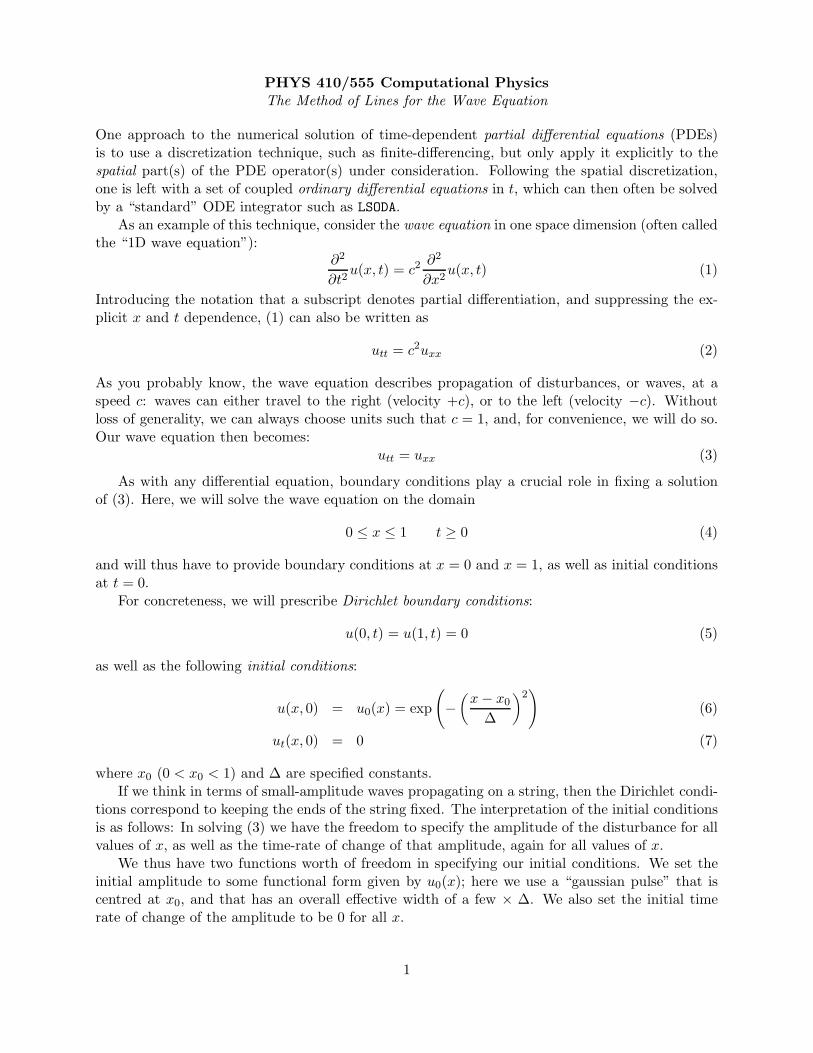
One approach to the numerical solution of time-dependent partial differential equations (PDEs)is to use a discretization technique, such as finite-differencing, but only apply it explicitly to thespatial part(s) of the PDE operator(s) under consideration. Following the spatial discretization,one is left with a set of coupled ordinary differential equations in t, which can then often be solvedby a “standard” ODE integrator such as LSODA.

As an example of this technique, consider the wave equation in one space dimension (often calledthe “1D wave equation”):

∂2

∂t2u(x, t) = c2

∂2

∂x2u(x, t) (1)

Introducing the notation that a subscript denotes partial differentiation, and suppressing the ex-plicit x and t dependence, (1) can also be written as

utt = c2uxx (2)

As you probably know, the wave equation describes propagation of disturbances, or waves, at aspeed c: waves can either travel to the right (velocity +c), or to the left (velocity −c). Withoutloss of generality, we can always choose units such that c = 1, and, for convenience, we will do so.Our wave equation then becomes:

utt = uxx (3)

As with any differential equation, boundary conditions play a crucial role in fixing a solutionof (3). Here, we will solve the wave equation on the domain

0 ≤ x ≤ 1 t ≥ 0 (4)

and will thus have to provide boundary conditions at x = 0 and x = 1, as well as initial conditionsat t = 0.

For concreteness, we will prescribe Dirichlet boundary conditions:

u(0, t) = u(1, t) = 0 (5)

as well as the following initial conditions:

u(x, 0) = u0(x) = exp

(

−(

x− x0

∆

)2)

(6)

ut(x, 0) = 0 (7)

where x0 (0 < x0 < 1) and ∆ are specified constants.If we think in terms of small-amplitude waves propagating on a string, then the Dirichlet condi-

tions correspond to keeping the ends of the string fixed. The interpretation of the initial conditionsis as follows: In solving (3) we have the freedom to specify the amplitude of the disturbance for allvalues of x, as well as the time-rate of change of that amplitude, again for all values of x.

We thus have two functions worth of freedom in specifying our initial conditions. We set theinitial amplitude to some functional form given by u0(x); here we use a “gaussian pulse” that iscentred at x0, and that has an overall effective width of a few × ∆. We also set the initial timerate of change of the amplitude to be 0 for all x.

1

Such data is known as time symmetric, since it defines an instant in the evolution of the waveequation where there is a t → −t symmetry. In other words, with time symmetric initial data, ifwe integrate backward in time, we will see exactly the same solution as a function of −t as we seeintegrating forward in time.

Since the wave equation describes propagating disturbances, and given that the initial conditionsare time symmetric, a little reflection might convince you that the initial conditions (6) and (7)must represent a superposition of equal amplitude right-moving and left-moving pulses. Thus, weshould expect the solution of (3), subject to (5), (6) and (7) to describe the propagation of twoequal-amplitude pulses that are initially coincident, but that subsequently move apart reflect offx = 0 and x = 1 respectively, move together, through each other, then apart, etc. etc. Indeed, thisis precisely the behaviour we will observe in our subsequent numerical solution.

As mentioned above, the method of lines, involves an explicit discretization only of the spatialpart of the PDE operator. Here we will use the familiar O(h2) finite-difference approach to thetreatment of uxx ≡ ∂2u/∂x2.

However, before proceeding to the spatial discretization, we first note that (3) is a second-order-in-time equation. In order that our approach eventually produce a set of first order ODEs in t, weintroduce an auxiliary variable, v(x, t),

v(x, t) ≡ ut(x, t) ≡∂u

∂t(x, t) (8)

and then rewrite (3) as the system:

ut = v (9)

vt = uxx (10)

The boundary conditions become

u(0, t) = u(1, t) = v(0, t) = v(1, t) = 0 (11)

while the initial conditions are now

u(x, 0) = u0(x) = exp

(

−(

x− x0

∆

)2)

(12)

v(x, 0) = 0 (13)

We can now proceed with the spatial discretization. To that end, we replace the continuumspatial domain 0 ≤ x ≤ 1 by a uniform finite difference mesh, xj:

xj ≡ (j − 1)h j = 1, 2, · · ·N h ≡ (N − 1)−1 (14)

and introduce the discrete unknowns, uj and vj:

uj ≡ uj(t) ≡ u(xj , t) (15)

vj ≡ vj(t) ≡ v(xj , t) (16)

Using the usual centred, O(h2) approximation for the second spatial derivative,

uxx(xj) =uj+1 − 2uj + uj−1

h2+O(h2) (17)

2

eqs. (9) and (10) become a set of 2(N − 2) coupled ODEs for the 2(N − 2) unknowns uj(t) andvj(t), j = 2, · · ·N − 1:

duj

dt= vj j = 2, · · ·N − 1 (18)

dvj

dt=

uj+1 − 2uj + uj−1

h2j = 2, · · ·N − 1 (19)

We can implement the Dirichlet boundary conditions as follows: if the boundary conditions aresatisfied at the initial time, t = 0, then they will be satisfied at all future times provided that thetime derivatives of u and v vanish at the boundaries. Using this observation, we can now writedown a complete set of 2N coupled ODEs in the 2N unknowns uj(t) and vj(t) which can then besolved using LSODA:

du1

dt= 0 (20)

duj

dt= vj j = 2, · · ·N − 1 (21)

duN

dt= 0 (22)

dv1dt

= 0 (23)

dvj

dt=

uj+1 − 2uj + uj−1

h2j = 2, · · ·N − 1 (24)

dvN

dt= 0 (25)

This solution procedure is implemented by the the program wave (See ∼phys410/ode/wave).You will follow an analogous approach to solve the diffusion equation in the final homework.

3

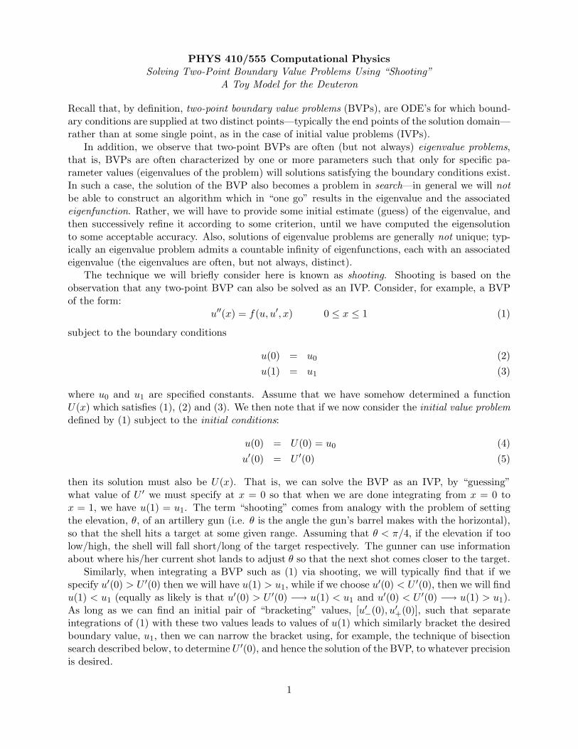
PHYS 410/555 Computational PhysicsSolving Two-Point Boundary Value Problems Using “Shooting”

A Toy Model for the Deuteron

Recall that, by definition, two-point boundary value problems (BVPs), are ODE’s for which bound-ary conditions are supplied at two distinct points—typically the end points of the solution domain—rather than at some single point, as in the case of initial value problems (IVPs).

In addition, we observe that two-point BVPs are often (but not always) eigenvalue problems,that is, BVPs are often characterized by one or more parameters such that only for specific pa-rameter values (eigenvalues of the problem) will solutions satisfying the boundary conditions exist.In such a case, the solution of the BVP also becomes a problem in search—in general we will notbe able to construct an algorithm which in “one go” results in the eigenvalue and the associatedeigenfunction. Rather, we will have to provide some initial estimate (guess) of the eigenvalue, andthen successively refine it according to some criterion, until we have computed the eigensolutionto some acceptable accuracy. Also, solutions of eigenvalue problems are generally not unique; typ-ically an eigenvalue problem admits a countable infinity of eigenfunctions, each with an associatedeigenvalue (the eigenvalues are often, but not always, distinct).

The technique we will briefly consider here is known as shooting. Shooting is based on theobservation that any two-point BVP can also be solved as an IVP. Consider, for example, a BVPof the form:

u′′(x) = f(u, u′, x) 0 ≤ x ≤ 1 (1)

subject to the boundary conditions

u(0) = u0 (2)

u(1) = u1 (3)

where u0 and u1 are specified constants. Assume that we have somehow determined a functionU(x) which satisfies (1), (2) and (3). We then note that if we now consider the initial value problemdefined by (1) subject to the initial conditions:

u(0) = U(0) = u0 (4)

u′(0) = U ′(0) (5)

then its solution must also be U(x). That is, we can solve the BVP as an IVP, by “guessing”what value of U ′ we must specify at x = 0 so that when we are done integrating from x = 0 tox = 1, we have u(1) = u1. The term “shooting” comes from analogy with the problem of settingthe elevation, θ, of an artillery gun (i.e. θ is the angle the gun’s barrel makes with the horizontal),so that the shell hits a target at some given range. Assuming that θ < π/4, if the elevation if toolow/high, the shell will fall short/long of the target respectively. The gunner can use informationabout where his/her current shot lands to adjust θ so that the next shot comes closer to the target.

Similarly, when integrating a BVP such as (1) via shooting, we will typically find that if wespecify u′(0) > U ′(0) then we will have u(1) > u1, while if we choose u′(0) < U ′(0), then we will findu(1) < u1 (equally as likely is that u′(0) > U ′(0) −→ u(1) < u1 and u′(0) < U ′(0) −→ u(1) > u1).As long as we can find an initial pair of “bracketing” values, [u′

−(0), u′+(0)], such that separate

integrations of (1) with these two values leads to values of u(1) which similarly bracket the desiredboundary value, u1, then we can narrow the bracket using, for example, the technique of bisectionsearch described below, to determine U ′(0), and hence the solution of the BVP, to whatever precisionis desired.

1

We note that it is not always an initial value per se which we tune in a shooting problem. Forsome second order BVPs (such as the one considered below), we can deduce a second initial valueat one of the boundary points (in addition to the one given by the boundary conditions) frommathematical or physical considerations, but, as discussed above, there is a parameter, λ, in thespecification of the BVP which must have certain values in order that the boundary condition atthe other boundary is satisfied. The idea is still the same; we look for an initial bracket [λ−, λ+]such that separate integration with the two parameter values gives end-point solution values whichare too small and too large respectively. We can then refine the bracket until we determine theeigenvalue and eigenfunction to the required precision.

We now illustrate this technique by using it to solve the toy model for a deuteron which isdiscussed in Chapter 9 of Mathematical Methods for Physicists by Arfken. A deuteron, as mostof you probably know, is a bound state of a proton and a neutron (the nucleus of deuterium, anisotope of hydrogen). The model is highly idealized; we assume that the deuteron wave function,ψ(~r), is a spherically symmetric solution of the time-independent Schrodinger equation, with theproton-neutron interaction described by a square wave potential.

Thus we wish to solve

− h2

2M∇2ψ(~r) + V (~r)ψ(~r) = Eψ(~r) (6)

where M is the deuteron “mass”, and E is the energy eigenvalue which will shortly become the“shooting parameter” in our BVP solution of the model.

From the assumption of spherical symmetry, we have

ψ(~r) → ψ(r) (7)

and

∇2ψ(r) =1

r2d

dr

(

r2dψ

dr

)

(8)

Further, definingu(r) ≡ rψ(r) (9)

we have (as you should verify)

∇2ψ(r) → 1

r

d2u(r)

dr2(10)

Thus, (6) can be rewritten:d2u(r)

dr2+

2M

h2(E − V (r)) u(r) = 0 (11)

As noted above, we will model the proton-neutron interaction as a finite-range square potential.Thus, we take

V (r) = V0 0 ≤ r ≤ a (12)

V (r) = 0 r > a (13)

where V0 is a negative constant, so |V0| is the depth of the potential well, while a is its width.As is the case for any solution of the Schrodinger equation, we must demand that our solution

of (6) be normalizable, i.e. that∫

ψψ∗dV = 1 (14)

2

so that there is unit probability that our deuteron is found somewhere in the universe. In thecurrent spherically symmetric case this means that we must have

4π

∫

∞

0r2ψ(r)2dr = 4π

∫

∞

0u(r)2dr = 1 (15)

Clearly, a necessary condition for normalizability is that

limr→∞

u(r) = 0 (16)

and this, in fact, is one of the boundary conditions for our ODE. Furthermore, we assert that forfixed values of the parameters of the model (a, M and V0), a normalizable solution will only existfor certain discrete values of E—the eigenvalues of our Schrodinger equation.

Before we consider the solution of (11) using shooting, we rewrite the equation in an equivalentform in which the minimum number of free parameters (which, if desired, can be made explicitlydimensionless) becomes evident. To this end, we define a rescaled radial coordinate, x

x ≡√

2Mr (17)

so that, among other things, we have

d2u

dr2→ 2M

d2u

dx2(18)

Further, we choose units such that h = 1 and V0 = −1 (you should establish that this is alwayspossible if it isn’t immediately obvious to you).

With these choices, we are left with one free parameter—the width, a, of the potential well.Given that we have adopted the rescaled radial coordinate x, it is more convenient to use x0, definedby

x0 ≡√

2Ma (19)

as the free parameter.Thus, our Schrodinger equation (11) becomes

d2u(x)

dx2+ (E − V (x)) u(x) = 0 (20)

where

V (x) = −1 0 ≤ x ≤ x0 (21)

V (x) = 0 x > x0 (22)

and where we again note that E = E(x0) is an eigenvalue of (20); i.e., for a given value of x0, onlyfor discrete values of E will we have a normalizable wave function.

The boundary conditions for (20) are derived from the demands that

1. ψ(r) be regular (analytic) at r = 0.

2. limr→∞ u(r) = 0.

The regularity condition at r = 0 means that ψ(r) admits an expansion

limr→0

ψ(r) = ψ0 + r2ψ2 +O(r4) (23)

3

where the ψi are constants (the power series expansion cannot have terms which are odd in r, sinceψ(r) would not have a well-defined derivative at r = 0 in that case). From this, it follows that u(r)has an expansion

limr→0

u(r) = rψ(r) = rψ0 + r3ψ2 +O(r5) (24)

Thus, we have

u(0) = 0 (25)

du

dr(0) = ψ0 (26)

We now observe that (6) (like all Schrodinger equations) is linear; given any solution, ψ(r) wehave that cψ(r), where c is an arbitrary positive constant, is also a solution. The particular solutionwe seek is fixed by the normalization condition:

∫

ψψ∗dV = 1 (27)

Operationally, this means that we can choose ψ(0) arbitrarily (say ψ(0) = 1 for convenience), then,for specified x0, vary E until we find a solution which satisfies

limr→∞

u(r) = limr→∞

rψ(r) = 0 (28)

(In other words, the eigenvalue is independent of the normalization of the eigenfunction).In preparation for a solution of our problem using LSODA we rewrite (20) in canonical first order

form by introducing

w(x) ≡ du(x)

dx(29)

We then have

du(x)

dx= w(x) (30)

dw(x)

dx= (V (x) − E)u(x) (31)

subject to

u(0) = 0 (32)

w(0) = 1 (33)

and with E to be determined so thatlim

x→∞

u(x) = 0 (34)

We will now assume that for any given value of x0, we are able to determine values E− and E+

(perhaps by trial-and-error) such that

limx→∞

u(x;E−) = −∞ (35)

limx→∞

u(x;E+) = +∞ (36)

where the notation u(x;Ei) means the trial solution u(x) computed using eigenvalue estimate Ei.We further assume that properties (35) and (36) hold for any values EHI and ELO that bracket thedesired eigenvalue, namely:

limx→∞

u(x;ELO) = −∞ (37)

limx→∞

u(x;EHI) = +∞ (38)

4

with eitherELO < E < EHI (39)

orEHI < E < ELO (40)

Given the initial bracket [E−, E+], then, we can compute the desired eigenvalue, E, accurate tosome desired tolerance δ, using a bisection search (also known as a binary search). Here is a typicalimplementation of a bisection search written in pseudo-code:

ELO := E−

EHI := E+

while |EHI − ELO| > δ do

EMID := (EHI + ELO)/2if u(x;EMID) → +∞ as x→ ∞ then

EHI := EMID

else

ELO := EMID

end if

end while

E := EMID

We note that the convergence rate of the bisection search is completely pre-determined; the sizeof the bracketing interval after n bisections is

1

2n(E+ − E−) (41)

The solution of equations (30)-(33) using LSODA is implemented as the program deut.f; thebisection search for the eigenvalues E(x0) is implemented via the shell-script Shoot-deut, whichitself uses the following collection of scripts which can be used to implement shell-level bisectionsearches:

bsnew <lo> <hi> # Initializes a new search

bscurr # Returns the current (mid) value for the search

bslo # Replaces the low bracket value with ‘bscurr‘

bshi # Replaces the high bracket value with ‘bscurr‘

bsdone [<tol>] # Returns completion code 0 if search bracket

# has been narrowed to a relative precision <tol>

# (which defaults to 10(-14), returns completion

# code 1 otherwise

bsnotdone [<tol>] # Logical negation of bsdone.

In practice, of course, we do not (can not!) integrate all the way to x = ∞, instead, we integrateto some finite x = xmax where xmax is chosen sufficiently large so that, for the specfied convergencecriterion δ, we can determine for all possible E whether the solution u(x;E) is diverging to +∞ orto −∞ at x = xmax.

Finally, as with many of the problems we have discussed in this course, the toy deuteron problemcan be solved “analytically”—however, as in the cases of those other exactly soluble problems we

5

have discussed, the numerical technique which we use to approximately solve this BVP can beextended very easily to solve entire classes of problems which are not amenable to exact solution.

6