Sensitivity of a Cloud-Resolving Model to the Bulk and Explicit Bin Microphysical Schemes.

Part I: Validations with a PRE-STORM Case

Xiaowen Li', Wei-Kuo Tao2, Alexander P. Khain3, Joanne Simpson2, and Daniel E. Johnson'

'Goddard Earth Science and Technology Center University of Maryland, Baltimore County

Baltimore, MD, USA

Laboratory for Atmosphere NASA Goddard Space Flight Center

Greenbelt, MD, USA

2

3The Hebrew University of Jerusalem Jerusalem, Israel

Submitted to Journal of the Atmospheric Sciences

June, 2004

https://ntrs.nasa.gov/search.jsp?R=20040171684 2018-07-15T04:17:51+00:00Z

Abstract

A cloud-resolving model is used to study sensitivities of two different

microphysical schemes, one is the bulk type, and the other is an explicit bin scheme, in

simulating a mid-latitude squall line case (PRE-STORM, June 10-1 1, 1985). Simulahons

using different microphysical schemes are compared with each other and also with the

observations. Both the bulk and bin models reproduce the general features during the

developing and mature stage of the system. The leading convective zone, the trailing

stratiform region, the horizontal wind flow patterns, pressure perturbation associated with

the storm dynamics, and the cool pool in front of the system all agree well with the

observations. Both the observations and the bulk scheme simulation serve as validations

for the newly incorporated bin scheme. However, it i s also shown that, the bulk and bin

simulations have distinct differences, most notably in the stratiform region. Weak

convective cells exist in the stratiform region in the bulk simulation, but not in the bin

simulation. These weak convective cells in the stratiform region are remnants of the

previous stronger convections at the leading edge of the system. The bin simulation, on

the other hand, has a horizontally homogeneous stratiform cloud structure, which agrees

better with the observations. Preliminary examinations of the downdraft core strength, the

potential temperature perturbation, and the evaporative cooling rate show that the

differences between the bulk and bin models are due mainly to the stronger low-level

evaporative cooling in convective zone simulated in the bulk model. Further quantitative

analysis and sensitivity tests for this case using both the bulk and bin models will be

presented in a companion paper.

2

3

‘Biz7, or ‘spectra! biz’ sche~lles, have h e e ~ widely used in theoretical microphysics

studes. They were also the natural choice in many early cloud models, whose dynamics were

relatively simple and whose simulations did not involve any ice phase microphysics (e.g.,

Clark 1973; Soong 1974; Takahashi 1975). A bin scheme uses dozens, even hundreds of

particle size bins to represent the drop size distribution of each hydrometeor type explicitly.

Although more realistic compared with both bulk and two-moment schemes, bin schemes are

computationally expensive and involve many uncertainties associated with detailed

microphysical processes. Because of the complexity of bin schemes, together with the

constraint of computer power, the success of the bulk type scheme in reproducing cloud

dynamics in numerical models, and the shrinking funding toward basic research on cloud

microphysics, the development of bin schemes in cloud-resolving models has been rather slow.

A handful of bin schemes with both water and ice phase microphysics has been incorporated

into cloud models (e.g., Hall 1980; Reisin et al. 1996; Khain and Sednev 1996; Ovtchinnikov

and Kogan 2000). Hall (1980) incorporated a bin scheme to a 2-D slab model to simulate the

impact of initial Cloud Condensation Nuclei (CCN) concentration on precipitation processes in

a single convection. The model developed by Reisin et al. (1996) has been applied recently to

the study of weather modification (e.g., Yin et al. 2000a) and the effects of giant CCN on

convective cloud development. (Yin et al. 2000b). Ovtchinnikov et al. (2000) used their 3-D

bin scheme cloud model to study ice production mechanisms in a small cumulus in New

Mexico. Khain et al. (1999) used a 2-D cloud model with a bin microphysical scheme to study

cloud-aerosol interaction in rain events in the Mediterranean.

A crucial question for cloud-resolving models using bin schemes is how it differs

from the widely used bulk schemes. How do different microphysical schemes interact with

4

cloud a d precipitation dynm~ics? In the early stages of cloud-resolving model development,

Soong (1974) and Shiino (1983) used axisymmetric models to study the sensitivity of their

models to bulk and bin schemes. Their models have warm rain microphysics only. They found

that using different microphysical schemes resulted in significantly different cloud structures,

cloud dynamics, and rain efficiencies. Soong (1974) also pointed out that even by varying the

parameters, their bulk scheme could reproduce only certain features simulated by the bin

scheme. Thus the bulk scheme could not substitute for the bin scheme by tuning its parameters,

even for the relatively simple warm rain process in his case.

This paper presents a detailed comparison between bulk and bin microphysical

schemes with both warm rain and ice microphsyics. The improved version of bin

microphysical scheme in Hebrew University Cloud Model (HUCM) (Khain and Sednev 1996)

is incorporated into the Goddard Cumulus Ensemble (GCE) model to study the sensitivity of a

cloud-resolving model to different microphysical schemes. Another goal of this paper is to

validate the newly incorporated bin scheme in the GCE model, with both previously available

bulk scheme simulations and observations of a continental Mesoscale Convective System

(MCS). In the next section, a brief description of both the GCE model and the HUCM bin

microphysical scheme is given, together with a general description of June 10-11 PRE-

STORM (the Preliminary Regional Experiment for Storm-scale Operational and Research

Meteorology) case simulated in this paper. Detailed comparisons of both model simulations

and observations are presented in section 3. The emphasis in section 3 is to identify major

dfferences between the bulk and bin scheme simulations that can be directly compared to

observations. Qualitative explanations of different model behaviors of the bulk and bin

simulations are given in both section 3 and in a dmussion in section 4. Further substantiation

5

of the thcorjr in sectizn 4 wi!! be presented in a cnmpaninn paper through different sensitivity

tests using both the bulk and bin schemes. Finally, a summary and conclusions are given in

section 5.

2. Model and case descriptions

2.1 GCE Model

A 2-D version of the GCE model is used in this study due to computational

limitations. Dynamics in the GCE model are anelastic. The subgrid-scale turbulence is based

on Klemp and Wilhelmson (1978). The bulk scheme in GCE model includes cloud water, rain,

ice, snow and hail as described in Lin et al. (1983). The selection of the microphysical

variables and parameters in the bulk scheme are suitable for the strong continental convections.

Both solar and infrared rahation parameterizations are included in the model (Tao et al. 1996).

All scalar variables use forward time and a positive, definite advection scheme with a non-

oscillatory option (Smolarkiewicz and Grabowski, 1990). More details on the GCE model can

be found in Tao and Simpson (1993a) and Tao et al. (2003).

2.2 HUCM Bin Scheme

The bin microphysical scheme in the HUCM explicitly describes the size

distributions of seven hydrometeor types: cloud/rain, three types of ice (plate, column and

branch), snow, graupel, and hail/frozen drops, as well as CCN. Each type has 33 size bins.

Nucleation of CCN, ice nucleation, diffusional growth (condensation, evaporation, deposition,

and sublimation) of all hydrometeors, freezing of water drops, an explicit description of ice

particle melting, drop-drop, drop-ice, and ice-ice collisiodcoalescence are represented in this

6

“ufi schzme. Detai!s ~f the bin scheme c m be fmnd in F-biifi ir?d Sednev (1996) and Khain et

al. (2000).

2.3 Experiment Design

The June 10-11, 1985 PRE-STORM case was a very well documented midlatitude

mesoscale squall line (e.g., Johnson and Hamilton 1988; Ruteledge et al. 1988). The GCE

model was initialized with a single sounding taken ahead of the newly forming squall line.

There are 33 stretched vertical levels, with a resolution of 240 m at the lowest level and 1250

m at the top. The horizontal grid number is 1024, with 1 km resolution for the center 872

points. The outer grids are stretched. The total integration time is 12 hours with a 6 s time step.

A lower level cool pool is applied for the first 10 minutes to initialize the convection. A

modified horizontal wind profile with lower level shears is also applied. Further details of the

experiment design for bulk scheme simulation can be found in Tao et al. (1993b).

Bin microphysics simulation uses exactly the same model settings a sdescribed above.

The only difference is in the microphysical scheme. The initial aerosol concentration and size

distribution are those of a clean continental background, with a small size CCN tail and no

large CCN above 0.4 pm. The CCN concentration at super saturation of 1% is 600 ~ r n - ~ .

3. Comparisons

The bulk and bin simulations show many similar features, especially in terms of the

system development. In both simulations, rain produced by a deep convective cell reaches the

surface within about 20 minutes. New convections are then regenerated in front of the old cell,

and the whole system propagates forward. Stratiform rain starts to form to the rear of the

leading edge by the end of the second hour for the bulk scheme and earlier for the bin scheme.

7

The j t i z ~ f c r z regim keeps expax!ing with the evohtinn of the system- Maximum stratifoim

rain area is achieved after 6 to 7 hours and the system becomes quasi-steady after that, with

regenerating convections at the leading edge and lighter stratiform rain trailing. The system

simulated by the bulk scheme moves faster compared with the bin scheme. The system

development simulated with both the bulk and bin scheme agrees well with the PRE-STORM

case observations, as well as the initial and mature stages of a typical continentaI MCS. In

conclusion, the newly incorporated bin scheme in the GCE model captures the developing and

mature stage of a PRE-STORM MCS realistically, similar to the simulation of the well-

accepted bulk scheme. No dissipation stage is simulated in this case because of the constant

environmental conditions in the model.

In the rest of this section, more detailed comparisons between the bulk and bin

models and observations are presented with the emphasis on the sensitivities of the model to

the different microphysical schemes. A direct comparison between model and observation is

very difficult due to limitations in both numerical modeling and field observations. While

efforts have been made in this paper to use observations to validate model performance, the

results should be considered only qualitative.

3.1 Radar Reflectivity

Radar reflectivity in the bulk model is calculated using parameterization according to

Rutledge and Hobbs (1984). In the bin model, it is explicitly calculated according to particles’

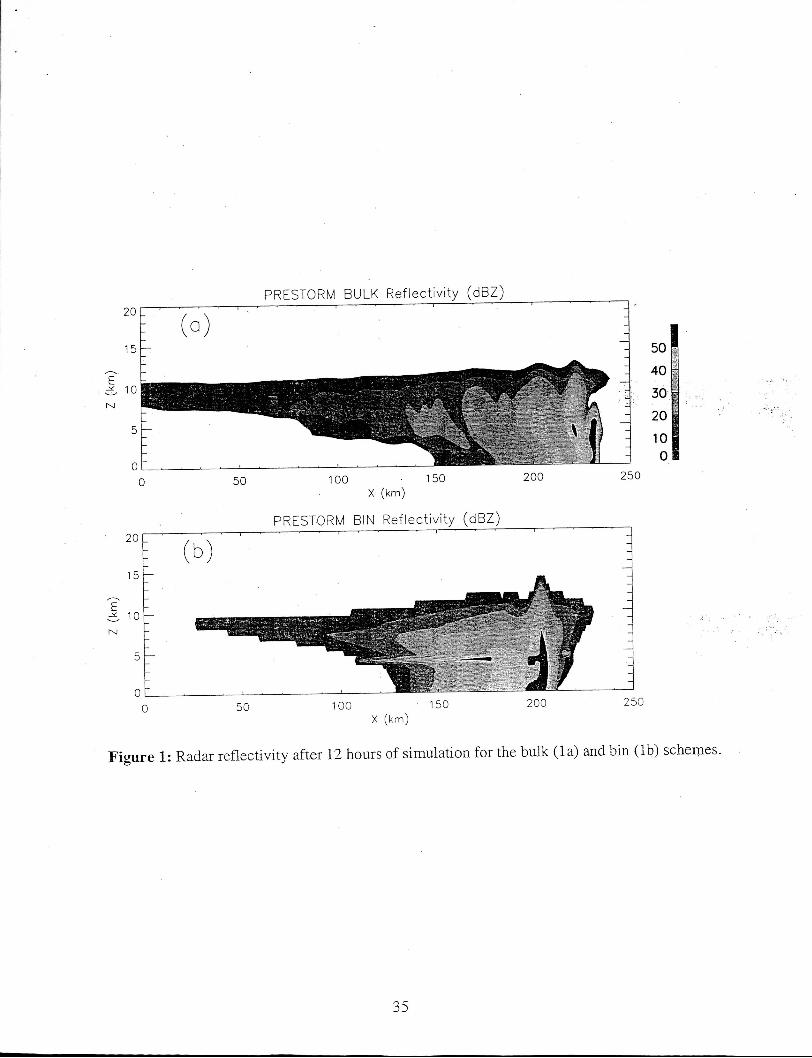
size distributions and densities. Figure 1 shows the radar reflectivity pattern at the end of the

12-hour simulations for the bulk (fig. l& and bin (fig. lb) models. Both figures have a leading

convective edge and a large area of trailing stratiform rain, a signature feature of MCSs.

8

m 1 - - - - - A -----L.n..t rl'ffnrn h n t x r l n n n f i m i r + S 1 a and l h is i~ their stra.tifom region. 1 Ilt: I U U ~ L pluuuiic.uL u i L i u L I l b u U ~ L V V ~ U A I A A ~ - ~ ~

The bulk simulation generally has vertical structures throughout the stratiform region,

reflecting remnants of consecutive convective cells moving away from the leading edge into

the trailing stratiform region. At this specific time, a dissipating convective core is identifiable

by a high radar reflectivity center in fig. l a around 80 km (x=150 km) behind the leading edge

of the system. The stratiform region in the bin simulation (fig. lb) is relatively homogeneous in

.horizontal direction compared with the bulk simulation. The convection cells dissipate very

quickly after they move away from the leading edge. No vertical cellular structure is visible in

the stratiform region in fig. lb. Although only one instant radar reflectivity pattern was plotted

in fig. 1 for each case, the above-described feature is consistent in radar reflectivity pattern

throughout the whole simulation.

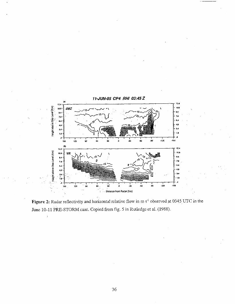
Radar reflectivity observations of June 10-1 1 PRE-STORM case have been described

in many papers (e.g., Smull and Houze 1987a,b; Rutledge et al. 1988; Biggerstaff and Houze

1993). Figure 2 is taken from Rutledge et al. (1988). It shows one RHI scan during the mature

stage of the June 10-1 1 PRE-STORM MCS. The leading convective zone and the large trailing

stratiform region shown in fig. 2 qualitatively agree with modeled radar reflectivity pattern in

both figures l a and lb. However, the horizontally homogeneous stratiform region simulated by

the bin model compares better with the observation than the bulk model. In the bulk

simulation, weak convective cells are identifiable well into the stratiform region, as shown in

fig. l a at x=150 km and x=180 km. Convective cells inside stratiform region have not been

observed in June 10-11 PRESTORM-case (e.g. Rutledge et al. 1988; Rutledge and

MacGorman 1988; Biggerstaff and Houze 1993). As a matter of fact, Rutledge et al. (1988)

described in their paper how the CP-4 radar was placed into a vertical mode right after the

9

feature was reported in the June 10-1 1 PRE-STORM case. Convective cells embedded aloft in

the stratiform region have been observed in other systems, e.g., Hobbs and Locatelli (1978),

Businger and Hobbs (1987). To .what extent they exist in continental MCSs is not clear. In this

particular PRE-STORM case, there is no observational evidence supporting the existence of

convective cells embedded in the stratifom region.

Differences in radar reflectivity patterns also exist in the leading convective zone

when different microphysical schemes are used. In the bulk simulation, the height of the first

convective cell is generally below 8 km in the mature stage. When the first cell reaches about 8

km, a new cell normally forms in front of it, cutting off its surface inflow. The original cell

(now the second cell) continues to grow to above 12 km and usually is the tallest cell. In the

bin model, the leading cell is always the tallest. New cells form close to the old cell,

maintaining a strong updraft core at the leading edge which continuously progresses forward.

Once the old cell leaves the leading updraft core, it quickly dissipates without further growth.

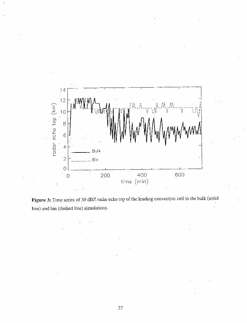
Figure 3 shows time series of the height of the 30 dBZ echo top of the first convective cell for

both the bulk (solid line) and bin (dotted line) simulations. In the early developing stage, both

bulk and bin simulations have deep leading cells reaching above 1Okm. After the systems

mature at around 350 minutes, the 30 dBZ radar echo top of the leading cell in the bulk

simulation seldom exceeds 8km, whereas the bin model produces much hgher echo tops. The

radar observation in fig. 2 has its leading cell as the tallest, followed by a much weaker second

cell. No radar pattern similar to fig. l a has been found in the literature regarding the June 10-1 1

PRESTORM case. However, a shallow leading convective cell with taller second and third

10

ceiis similar to h e buiic siiiydiition in fig. :a has Seex observed in ether ,MCEs. (e.g., Ch_ong et

al. 1987). Again, bin scheme does a better job in replicating the radar reflectivity patters in the

convective zone in this case study.

A prominent bright band exists in the observation in fig. 2, with its maximum

reflectivity located around 3.5 km. The bin model successfully reproduces this feature, as

shown in fig. lb. The maximum reflectivity band is about 500m higher and has larger values

than the observation in fig. 2 because of the simplification used in calculating radar

reflectivities of mixed phase particles. It was simply assumed that the melting particles had a

water coating so the refractive index for water was used for them. In reality, water rarely forms

a coating around large particles. Instead the water is held in the ice interstices, forming a

mixture of water, ice and air (Fujiyoshi 1986). According to the aircraft measurements of the

same PRE-STORM system reported by Willis and Heymsfield (1989), the 0°C level in

stratiform region was indeed around 4 km. Their study shows that a few large aggregates

survived as ice to as warm as +5"C, which is another reason for the maximum bright band

being below the 0°C level. The bulk model totally missed the bright band in the stratiform

region despite the fact that the same simplification used in the bin model was used for bulk

model calculations. Part of the reason is that the convective cells in the stratiform region in

bulk simulation continuously transport water drops above the melting level, smearing out the

melting signature in the radar reflectivity. Other possible reasons are: the coarse treatment of

melting in the bulk microphysical scheme, and the fact that the bulk scheme has only high-

density, fast-falling hail, whereas the bin scheme considers both hail and graupel. Falling snow

contributes to the bright band in both bulk and bin simulations..However, its effect is relatively

small because of its relatively low concentration in the stratiform region.

11

Several discrep~ncies exist for hnth hiilk and bin simulations when compared with

observations. For example, modeled radar reflectivities are higher than the observations in the

convective region. The highest reflectivity measured in the leading convective core is about 50

dBZ, whereas the highest core reflectivities in both the bulk and bin simulations are all above

5OdBZ. There are two possible reasons for the overestimation of radar reflectivity. First, the

convection is too strong in numerical simulations. Since the direct measurement of vertical

velocities in convective cores are very difficult, and indirect calculations (e.g., Rutledge and

MacGorman, 1988) do not have enough resolution for the convective cells, this possibility

remains an open issue. Second, the assumed particle size distribution could be too large in the

bulk model. And the bin scheme could be producing excessive large particles. Since the bin

microphysical scheme does not include raindrop breakup, this contributes at least partly to the

higher radar reflectivities in the bin simulation. Another discrepancy with the observations is

the lack of a transition zone near the surface between the convective and stratiform region in

the models. A transition zone is a gap usually 10-30km wide with lowest radar reflectivity in

the middle to lower atmosphere as shown in fig. 2 between -15 and -50 km. It has been widely

observed in other squall-line systems. Biggerstaff and Houze (1993) analyzed the transition

zone in the 10-11 June 1985 PRE-STORM system and concluded that the major contribution to

its formation is the lack of small ice crystals in this zone caused by the downdrafts. Less

aggregation leads to reduced rainfall in this region compared with the stratiform region.

Further model development is needed in order to resolve this issue. Thirdly, the stratiform rain

area in both models is relatively narrower compared with observations. The lack of stratiform

rain exists in many other case studies using cloud-resolving models. This might be related to

the lack of synoptic-scale forcing in the model settings.

12

3.2 Sulface Rainfall

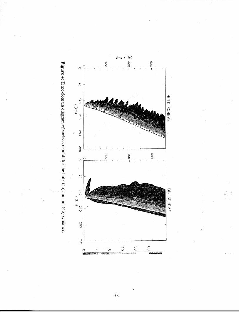
For 2-D simulations, time-domain contours as shown in fig. 4 provide a

comprehensive picture of surface rainfall evolution. The bulk and bin schemes show very

different surface rainfall patterns in fig. 4. The bulk model produces an oscillating surface

rainfall with evidence of the rearward propagating convective cells clearly identifiable as high

surface rainfall streaks. The bin scheme, on the other hand, shows a smooth surface rainfall

pattern in fig. 4b. The leading convection merges quickly into the stratiform region with little

evidence of rearward propagation in the surface rainfall. The trailing rain area in the bin

simulation is larger than the bulk simulation. Instantaneous surface rainfall seldom exceeds 100

mm hr" in the bin simulation, while the bulk scheme consistently shows areas of surface

rainfall of more than 100 mm hr-'. The slopes of the leading edge lines in fig. 4 indicate that the

system simulated with the bulk scheme propagates faster than the bin simulation. There is a

strip of light rain immediately ahead of the convective region in the bin simulation (the forward

overhang of the light precipitation), whereas there is little forward overhang in the bulk

simulation. The observed radar reflectivity in fig. 2a does show a small, light rain strip in front

of the leading convective edge. Radar composites for the same case described in Biggerstaff

and Houze (1993) and Smull and Houze (1987a) support the existence of a forward overhang

in the June 10-11 PRESTORM case, too.

The anvil stratiform rain trailing the convective line in MCSs contributes significantly

to both the total surface rainfall and the mesoscale dynamics (e.g. Houze 1993). Two methods

(Le., Johnson and Hamilton 1988 (JH_88), and Churchill and Houze 1984 (CH-84)) are used

in this study to separate stratiform and convective rain. The JH-88 method is used as a direct

comparison with their PRE-STORM observations. CH-84 is a more widely used separation

13

method and is listed for cornpaison. The resuks are shown in tab!. 1. Johncnn and Hamilton

(1988)'s stratiform percentage was calculated using densely deployed 5-minute rain gauge data

collected during the passage of June 10-11 PRE-STORM squall line. Convective rain is

assigned when the rainfall rate is above 6 mm hf'. When it falls below 6 mm hi ' , the rain is

categorized as stratiform. The same 6 mm he' threshold is applied to instantaneous rainfall

rates sampled at 1-minute intervals in model simulations. Using the JH-88 method, the bin

scheme produces twice as much stratiform rain as the bulk scheme. However, both the bulk

and bin simulations underestimate the stratiform rain compared with Johnson and Hamilton

(1988) observation. The CH-84 method results much larger stratiform rain ratios for both the

bulk (16%) and bin (28%) simulations as shown in table 1.

I

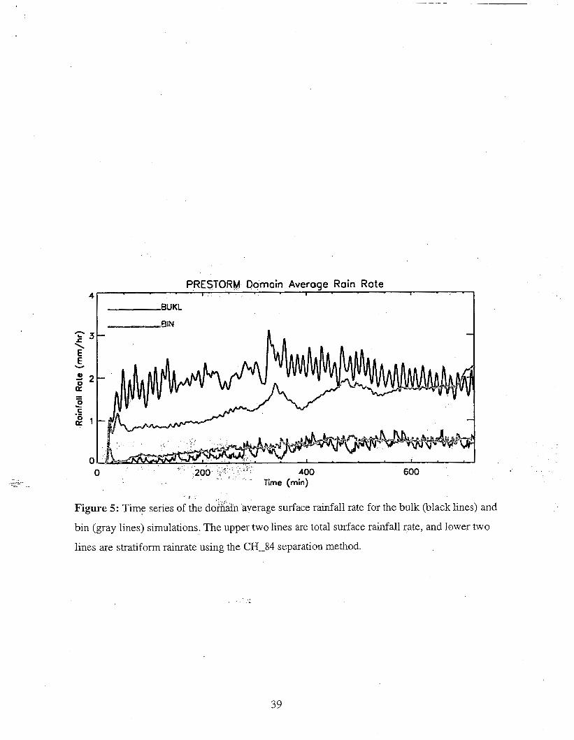
Figure 5 shows time series of domain-averaged surface rainfall for both the bulk

(black lines) and bin (gray lines) simulations. The upper two lines represent total rainfall rate;

The lower two lines represent stratiform rain rate using the CH-84 separation method. The

bulk scheme has a much larger temporal oscillation compared with the bin scheme, in both

total and stratiform rain. The average rainfall rates in bin model are less than bulk simulation

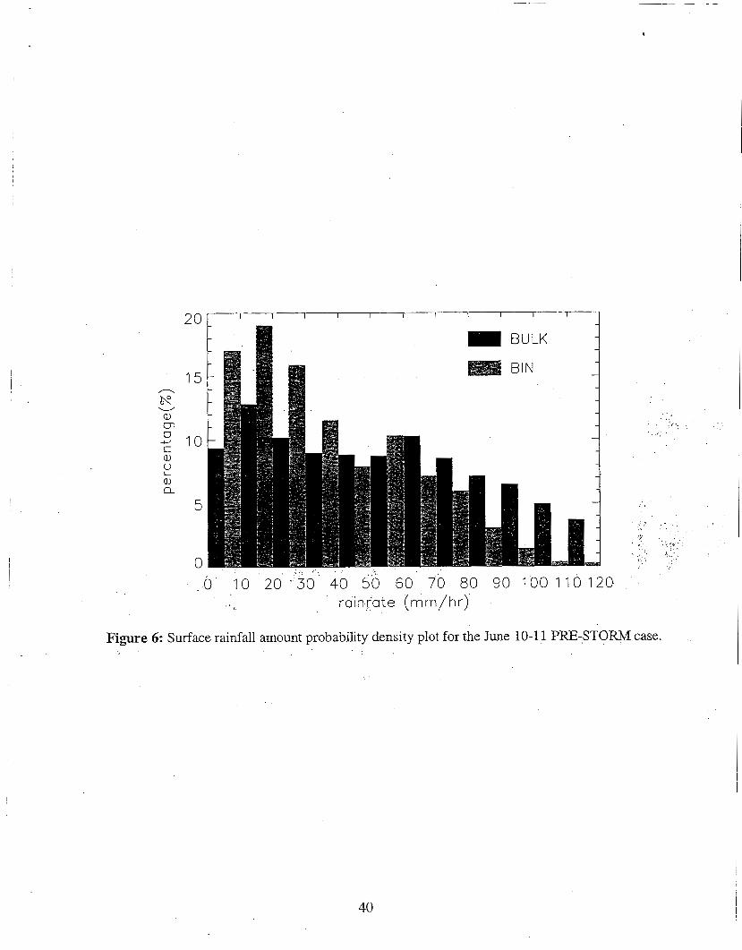
except for the last 1 hour when they become similar. Probability distributions of surface

rainfall are illustrated in fig. 6 where the percentage of the total rain amount is sorted by rain

rate bins. The bulk simulation produces a surface rain spectra that is relatively flat up until 60

mm hr-*, whereas the bin scheme has a large peak at smaller rainfall rates (less than 30 mm hr'

). The bulk scheme also has a higher tail of large rainfall rates compared with the bin scheme.

*

1

3.3 Kinematic Structure

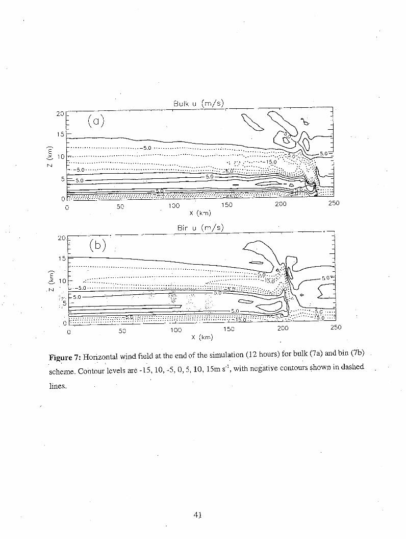
The horizontal wind fields of MCSs have many common features as described in,

e.g., Houze (1993). Figure 7 illustrates the instantaneous horizontal wind of the bulk (7a) and

14

1 . ,-I, \ Din ( / 0) sclieiiies st the cad of the 12 hour simdations relative to the MCS. Similar to many

previous observations and simulations of MCSs (see fig. 2b for an example), a deep front to

rear flow exists at mid to upper levels, fed by the strong outflow from convective cells at the

leading edge. This upper level outflow is responsible for carrying small ice particles rearward

into the stratiform region. Dominant at the low to mid levels is a rear to front flow maintained

mainly by evaporative cooling and water loading (Smull and Houze 1987b; Zhang and Gao

1989). A near surface front to rear flow prevails below 1.5 km. Both the model simulations

shown in fig. 7 have similar horizontal wind structures and magnitudes compared with the

observation in fig. 2b.

Several differences exist between the models and the observation. The observed rear

to front inflow originates higher (above 9 km) than both simulations (below 8 km). The

observed rear inflow in fig. 2b has an obvious downward slope that is lacking in both of the

simulations. In the bulk simulation, the rear inflow descends to the surface after it enters the

convective region, but it lowers down only slightly and never touches the ground in the bin

simulation. The lack of a realistic large-scale environment for the current cloud-resolving

model may explain the lower origin of the rear to front flow in the simulations. Zhang and Gao

(1989) successfully reproduced the observed rear inflow structure in 10-1 1 June PRE-STORM

case using a nested grid mesoscale model. Sensitivity tests in their study showed that when

evaporative cooling was turned off, the rear to front inflow still originated at about the same

height. But i t did not penetrate into the stratiform region. They argued that large-scale

baroclinity was responsible for the higher origin and partly the strength of the rear to front

inflow. The lowering of the rear to front flow near the convective region is related to the

relative strength of the positive vorticity generated by the cool pool at the rear side of the

15

convective region, and the negative vorticity produced by the Souyzixy-gradience of the rear

propagating convective cells, according to Weisman (1 992). The bin simulation produces

stronger upper level negative vorticity and weaker lower level positive vorticity compared with

the bulk simulations, resulting less lowering of the rear to front flow in the bin simulation.

More quantitative discussions will be given in a companion paper.

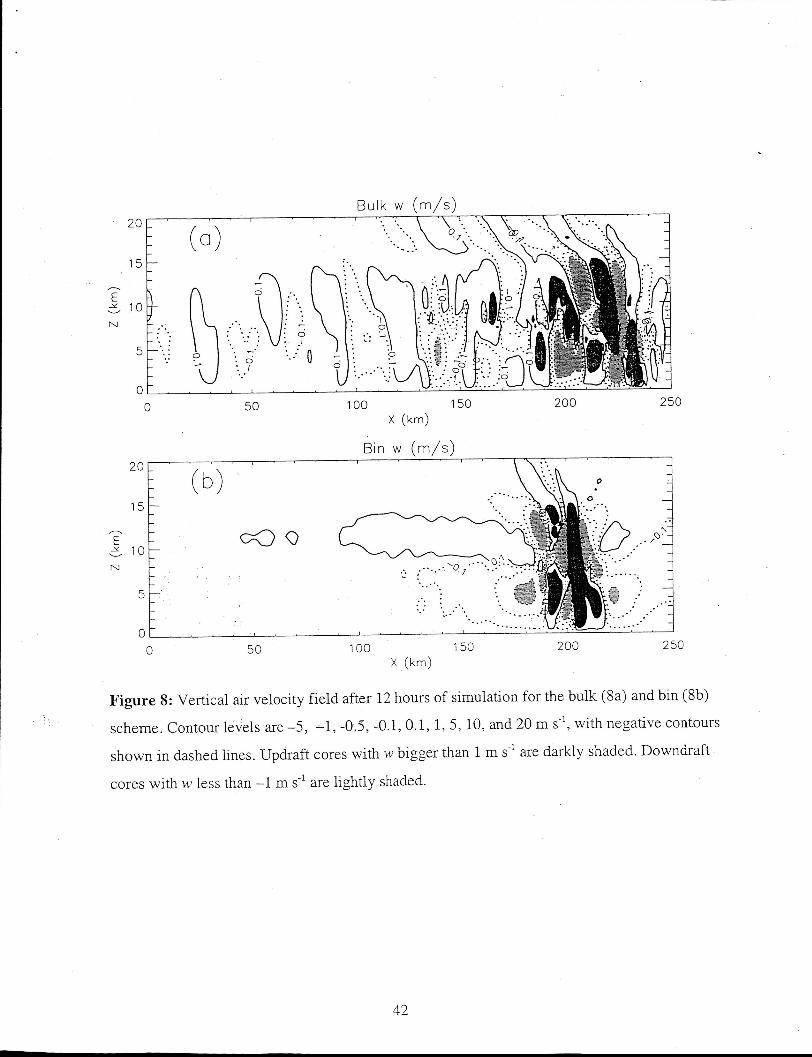
The instantaneous vertical air velocity (w) fields shown in fig. 8 are decisively

different between the bulk and bin simulations. The updraft cores, defined here as areas with w

stronger than 1 ms-', are darkly shaded. The downdraft cores stronger than -1 m s-' are lightly

shaded. There are more updraft cores in the bulk simulation (Sa) than in the bin simulation

(8b). In the bulk simulation, small updraft cores extend as far as 80 km from the leading edge.

These updraft cores are responsible for the convective cells in the stratiform region as shown in

fig. la. The bin simulation, however, has fewer updraft cores, and they are all w i h n 30 km of

the leading edge. The structures of the updraft cores in the bulk and bin simulations are

different, too. In the bin simulation in fig. Sb, a single updraft core at the leading edge extends

from the surface up to 15 km, with a slight rearward tilt. The air accelerates continuously along

the core and achieves a maximum velocity of more than 20 m s-' at around 8 km. The leading

updraft core in the bulk simulation is much shorter, reaching only about 8km. The maximum w

in fig. 8a is about 18 m s-' and is achieved at around 4 km. The second updraft core, which is

aIoft at x=225 km in figure 8a, extends to 15 km and is totally separated from the first core by a

downdraft core. Without continuous inflow from the surface, the air in the second core gains

less momentum compared with the single core structure in fig. 8b. This contributes to a smaller

maximum vertical air velocity in the bulk simulations as shown in fig. 9, a time series of the

maximum and minimum w in both the bulk (solid lines) and bin (dotted lines) simulations.

16

A!thoug!: the ,'~!aximum MI' is weaker in biilk simulation, its minimum w is strofiger due to

strong rain evaporation in the convective region compared with the bin simulation.

More comprehensive updraft core statistics dcring the 12-hour simulation, including

the average updraft core size, mean vertical air velocity in the core ( W ) , and number of cores at

both 2 km and 8 km, are listed in table 2. The bulk scheme produces more, and slightly larger

updraft cores at both levels, again illustrating the backward propagation of the convective

celss. At 8 km, the average core strength in the bin simulation is 7 ms", compared to only 3.3

ms-' in the bulk scheme. This is consistent with the higher position of the maximum w in the

bin simulation'as shown in fig. 8.

Both single and dual-doppler radar analyses of the June 10-11 PRE-STORM case

have been performed to derive the vertical air velocities (e.g., Rutledge et al. 1988; Rutledge

and MacGorman 1988; Biggerstaff and Houze 1993). Comparable to the simulated

instantaneous w field in fig. 8 is a dual-doppler analysis shown in fig. 6 in Biggerstaff and

Houze (1993). The leading convective cell in their radar observation extends to above 13 km

with the maximum w of more than 14 ms-' located at around 9 km. There is no discontinuity on

the updraft core in their observations as shown in the bulk simulation in fig. 8a. These features,

and the higher location of the maximum w, compare favorably with the bin simulation.

The downdraft cores exist at both upper and lower levels, as shown in fig. 8. Lower-

level downdraft cores are driven mainly by evaporative cooling and water loading, and are of

interest in this study. As shown in fig. 8, lower-level downdraft cores immediately adjacent the

leading convection have very different strengths and sizes in the bulk and bin simulations. The

bulk simulation in fig. 8a shows an intense downdraft core of more than -5 m s-l located at

x=225 km. In the bin model, the downdraft core at around x=198 km in fig. 8b has a maximum

17

strength of only -2 ms-'. This downdraft core is nor; only weaii-eiin strength, but a!se smaller ir,

size compared with bulk simulation. This is consistent with the minimum w time series shown

in fig. 9, where time series of the minimum w below 5 km are plotted. These minimum w

represents the strongest lower level downdraft which normally occurs right behind the leading

convection. The downdrafts in the bulk model are always stronger, and have larger temporal

variations compared with the bin simulation. The reason is that in the bulk scheme, a large

amount of rain falls into the downdraft region due to the backward tilting of the first cell and

the formation of a second updraft core directly above the downdraft core. More evaporation

results in the bulk model compared with the more upright, continuous convective core

simulated in the bin model. The majority of the rain in the bin model falls within the leading

updraft core, resulting in a much smaller and less intense downdraft core immediateIy behind

the leading line.

Vertical air velocity structures in the stratiform region shown in fig. 8 are very

different too. The bin simulation has a nearly continuous weak updraft above 7km and

downdraft below it. The bulk simulation shows alternating updraft and downdraft in the

stratiform region, similar to its convective region, but with much weaker strengths and lower

frequencies.

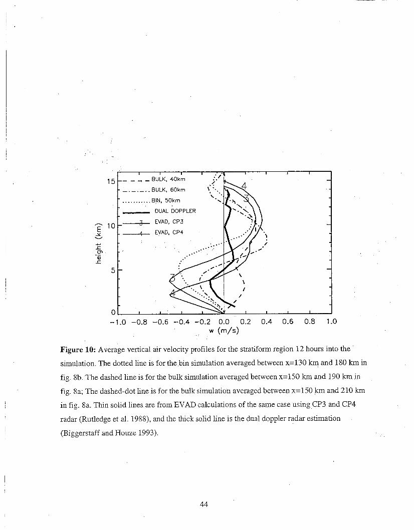
The previous observations have been focused on the domain-average vertical velocity

profiles in the stratiform region in MCSs, which show a very consistent pattern of weak

updraft/downdraft at upper/lower levels (see Houze, 1993 for a comprehensive review). In

order to compare model simulations with the observations, the simulated w profiles in the

stratiform region are plotted in fig. 10 using non-solid lines. These are the instantaneous

domain-average profiles at t=12 hours. In the bulk simulation, there are alternating updrafts

18

and downdrafts in stratiform region. Therefore tile ' - ~ I ~ J J C ~ -1----- VI -c+L. LIIc dVlllCLlll-Ll n--;n Q ' I I P T - ~ ~ T P vvAUbw nrnfilpc yA-A.+-- are _ _

very sensitive to the size and location of the domain specified. For example, starting from the

first grid at the rear of the system where surface reflectivity is larger than 0 dBZ (x-1-50 in fig.

l), different domain sizes are used to calculate the average profile for the bulk scheme. The

dashed line in fig. 10 is the average from x=150 to x=190 (40 km domain), and the dash-dot

line is the average from x=150 to x=210 (60 km domain). The average w at lower levels is

positive over the 40 km domain in the bulk case, which is contrary to all the observations.

However, when w are averaged over the 60 km domain, the profile becomes negative at lower

levels, because the large downdraft core at around x=200 km in fig. 10 is now included in the

calculation.

For the June 10-11 PRE-STORM case, average w profiles in the stratiform region

have been reported in Rutledge et al. (1988) using single doppler radar EVAD measurements,

and in Biggerstaff and Houze (1993) using dual-doppler radar analysis. Their results are

reproduced in fig. 10 in solid lines. The three observations agree with each other qualitatively,

but not quantitatively. The general structure and magnitude of the average updraftldowndraft in

both bin simulation and bulk simulation using 60 km domain average agree qualitatively with

observations. But dscrepancies do exist. Both CP3 and dual-doppler observations show a

maximum downdraft near the melting level. CP4 has a lower maximum downdraft. The w

profile in the bulk simulation for the 60 km domain has its maximum near the melting level.

The bin simulation produces a downdraft peak about 1.2 km above the melting level. This

indicates that significant sublimation occurs in the bin simulation above the melting level.

3.4 Pressure

19

n --d---Ln+:r.* C a l r l -t t-13 h m i r c ~ T P nlnttprj in f io 1 1 R rresbliie p ~ ~ ~ ~ l u a L l u l l Ilblus uL I.VULV ..-_ _ _ _ - - ~ . _ _ - oth the bulk and bin

models are able to capture some of the common features observed in the June 10-11

PRESTORM case. For example, a surface high-pressure center generated by the cool gust front

coincides with the arrival of strong convective rain for both bulk and bin simulations. This

agrees with the surface pressure observation described in Johnson and Hamilton (1988), where

in a single surface station, a pressure jump of 4 mb was observed, followed by heavy rain

within five minutes. The surface pressure jump in the bulk simulation is 2.2 mb, and it is 3.3

mb in the bin simulation. The bin simulation in fig. l l b shows a small pre-squall low at x=220

km.kA pre-squall low is reported in Johnson and Hamilton (1988) in their figure 13. The bulk

simulation does not have a pre-squall low center, nor is the pre-squall low a persistent feature

in the bin simulations. Both models show a meso-low with similar intensity at mid-levels of the

MCSs. This feature is consistent with the pressure perturbation field retrieved from the doppler

radar observations of the June 10-11 PRE-STORM case (Braun and Houze, 1994). Multiple

low centers exist in the bulk simulation (at x=190 km and 160 km) but not in the bin

simulation, presumably because of the multiple convective cells in bulk model. Neither the

bulk nor the bin model can reproduce the surface meso-low center to the rear of the system,

which was observed by Johnson and Hamilton (1988) and simulated by Zhang and Gao (1989).

This surface rear low is believed to be induced by the heating of the middle to low level

downdraft, which is also missing in the simulations, as shown in fig. 8. This may be part of the

reason for the lack of downward tilt in the mid-level rear to front flow as shown in fig. 7.

Generally, the cloud-resolving model can not reproduce pressure perturbation features

associated with large-scale dynamics, for example, the surface wake-low. However, both the

20

r- - L - - - - - -n---ntoA h,, l n p 9 ] d\rnnmirq bulk and bin schemes successfully simuiated pressux i e a i u m g G l l b l a L b u uJ lvvuI .- J **---- - - 7

such as the surface high before the leading edge and the mid-level meso-low center.

3.5 Thermodynamical and microphysical fields

In the previous sections, the radar reflectivity, surface rainfall, wind, and pressure

field simulated by both the bulk and bin models have been compared, with the emphasis on the

differences between the two microphysical schemes. These simulations were also compared

with the applicable observations. The instantaneous fields presented in previous sections are

representative of the later, quasi-steady stage (the last 6 hours) of the simulated storm. Time-

average plots tend to obscure features like the cellular structure of the vertical air velocity in

the bulk scheme when comparing with the observations. Although both the bulk and bin

models are able to reproduce many important features observed in the June 10-11 PRE-

STORM case, distinct differences exist between them. This shows the important role the

microphysical scheme plays in the cloud-resolving model. In the following sections,

mechanisms that produce the differences between the bulk and bin simulations will be

investigated by analyzing thermodynamical and microphysical outputs from the models.

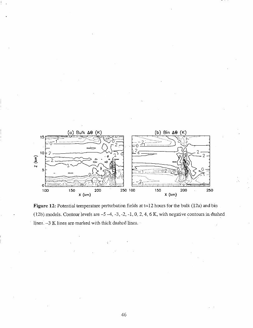
Figure 12 shows the instantaneous potential temperature perturbation at t=12 hours.

-3 K contour level is highlighted with thick dashed lines. Again the bulk and bin simulations

show distinct differences. The diabatic heating in the convective region is more organized in

the bin model (12b) due to its deeper and more organized updraft cores than the bulk model

(12a). The negative potential temperature perturbation at lower levels in the bin simulation is

deeper but less intense compared with the bulk simulation. In the bulk simulation, negative

potential temperature is mainly confined below 3 km in the rear part of the system, with a thick

head coinciding with the leading convection edge. This structure is similar to a density current

21

The minimum temperature is below -5 K in the cold head. The bin simulation has negative

potential temperature extending up to 5 km. A cool pool with a minimum potential temperature

of less than -4 K exists at the leading convection edge. However, the cool air does not spread

to the ground as the bulk model does. The potential temperature perturbation near the ground

in the rear part of the system is much warmer in the bin simulation (--1K) than in the bulk

simulation (--4K). Several factors may contribute to these differences. First, the rear to front

inflow in bulk model (fig. 7a) lowers to the ground near the leading edge, cutting off the near

surface front to rear flow. Warmer, unperturbed air in front of the system cannot reach the rear

of the system directly. Surface air at the rear part of the system comes mainly from

evaporatively cooled air from strong downdrafts in the convective zone. The bin model,

however, has a continuous front to rear near surface flow (fig. 7b). Some of the near surface air

at the rear of the system comes directly from the warm surface air in front of the system,

resulting to a warmer near surface potential temperature compared with the bulk model.

Secondly, evaporative cooling in the convective region, the major source of the cold air near

the ground, is much stronger in the bulk simulation. This can be inferred from the stronger,

broader downdraft cores in the convective region shown in fig. 8a. Third, sublimation above

the melting level is stronger in the bin simulation as inferred from both fig. 9 and fig. 10. This

contributes to the cooler air at middle levels and thus a thicker negative region in the bin

simulation. The potential temperature perturbation retrieval by Braun and Houze (1994)

showed a density current type of structure with the coolest air near the surface, similar to the

bulk simulation. More quantitatively comparison is difficult due to the assumptions and limited

resolutions in the retrieval.

22

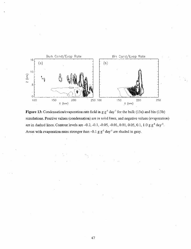
Direct evidence that evaporative cooling in rhe conveiiiv-e regioii is strcager In the

bulk simulation is shown in fig. 13, where the condensatiodevaporation rate contours in units

of g g-' day-' at t=12 hours are plotted. Condensation is shown in solid lines and evaporation in

dashed lines. Areas with evaporation rates stronger than -0.1 g g" day-' are shaded with gray.

Patches of condensatiodevaporation occur in the upper stratiform region in the bulk simulation

but not in the bin simulation. This is consistent with the existence of updraft cores in stratiform

region in fig. 8. Evaporation in the stratiform region is much stronger in the bin simulation as

shown by the size of the shaded area in the stratiform regions. The maximum evaporation rate

there is stronger than -0.2 g g-' day-' in the bin simulation, compared with just -0.1 g g-' day-'

in the bulk simulation. This contributes to the stronger average downdraft in the stratiform

region in the bin simulation as shown in fig. 10.

Contrary to the stratiform region evaporation described above, evaporation in the

convective zone in the bulk simulation (shaded between x=220 and 230 krn in fig. 13a) is much

broader compared with the bin simulation (shaded at around x=200 km in fig. 13b). The

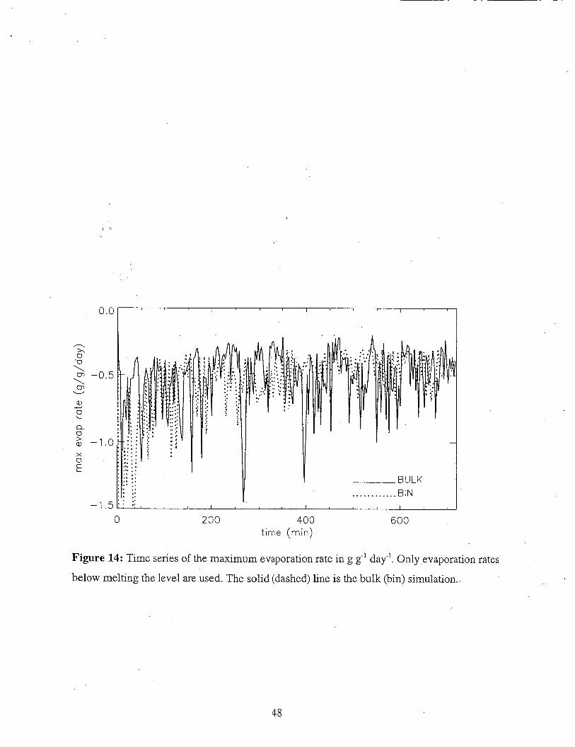
magnitude of the evaporation rate is similar for both models at this time. However, average

evaporation in the convective region is stronger in the bulk simulation as shown in fig. 14,

where time series of the strongest evaporation rate below the melting level for the bulk (solid

line) and bin (dotted line) mode1 are shown. During the quasi-steady state toward the later half

of the simulation, deep spikes of strongest evaporation rate happens in the bulk simulation, but

they are much weaker in the bin simulation. These spikes may cause the bore like structures in

the potential temperature perturbation shown in fig. 12a. For example, local potential

temperature minimum can be identified at x=220 km, x=190 km, x=160 km and x=135 km in

23

figure 12a. Th bin model has relatively less tenipoial iiarjliations ii; :he ,?.,axinurn evaporation

rate compared with bulk model during the latter half of the simulation.

4. Discussion

Both the bulk and bin microphysical models are able to successfully reproduce

general features observed in the June 10-11 PRE-STORM case. However, the model

simulations are very sensitive to different microphysical schemes. With identical model setup,

initial, and environmental conditions in the GCE model, two self-consistent microphysical

schemes produce very different details in the storm structure as discussed in the previous

sections. This indicates the importance of the microphysical scheme in the cloud-resolving

model. In this section, some general discussions to explain the model sensitivity to different

microphysical schemes are given. Further analysis and substantiation of these points will be

presented in a companion paper using sensitivity tests with both the bulk and bin models.

Diabatic heating/cooling is the key to cloud microphysics-dynamics interaction. In

this particular case study, different patterns and strengths of the evaporative cooling produced

by different microphysical schemes are largely responsible for their different structures. In the

convective region, the bulk scheme has stronger and broader evaporative cooling (fig. 13 and

14) during the mature stage of the system. This produces a stronger downdraft core (fig. 8) and

near surface coo1 pool (fig. 13) in the bulk model correspondingly. The near surface cool pool,

coupled with environmental wind shear and the strength of the rear to front inflow, is

responsible for the regeneration of new convective cells at the front of the system and the

sustaining of a forward moving, long-lasting squall line (e.g., Rotunno et al. 1988; Morris and

Rotunno 2004). The stronger cool pool (fig. 13) and downdraft (fig. 8) in the bulk scheme

produce a faster moving system compared with the bin simulation (figure 4). With the same

24

environmental wind shear, the stronger cool pool in buik simula~on fCjims a skzitim sirrdx tc!

the “less-than-optimal shear, but a long-lived state” in Rotunno et al. (1988). This type of

system is slanted upshear, as evident in the multiple cells in fig. la. The instantaneous vertical

velocity in the bulk simulation (fig. 8a) suggests that the slanted updraft core is cut off by a

deep downdraft core, generated by both evaporative cooling at lower levels and mechanical

forcing at upper levels. The residual updraft core moves continuously toward the rear of the

system while maintaining some of its buoyancy. This forms multiple convective cells

extending far behind convective line into the stratiform region. The bin simulation, on the other

hand, has a weaker cool pool and a more upright convective core at the leading edge. The

majority of its rain falls within its updraft core, resulting in less evaporation and a weaker cool

pool. The more upright leading convective core keeps the buoyant air within itself, forming a

stronger and tall updraft core, and larger maximum air velocity in the bin simulation (fig. 9).

When the air leaves the leading updraft core at the upper levels, it quickly loses its buoyancy

and forms the stratiform region. The majority of the stratiform rain in the bin simulation comes

from the ice particles transported rearward by the upper level flow. On the other hand, portion -

of stratiform rain in the bulk simulation still come from the condensation/deposition within the

residual updraft cores. More quantitative analysis will be discussed in a companion paper.

4. Summary and future work

The GCE model coupled with the HUCM explicit microphysical bin scheme is used

to simulate the June 10-11 PRE-STORM MCS. Simulations using both the bulk and the newly

incorporated bin microphysical scheme have successfully reproduced many features observed

in this case (e.g., the evolution of the system to the mature stage, the distribution of the

convective and stratiform rain, the horizontal flow structure, and the storm induced pressure

25

perturbation patterns). 'l'hese results serve as a validation for tilt: rubustiless of the b h schcme

in the long-term simulations of continental MCSs. However, the modeled cloud dynamics also

exhibit sensitivities to the different microphysical schemes, as evident in the many differences

between the bulk and bin models detailed in this paper. The most prominent difference occurs

in the stratiform region. In the bulk simulation, convective cell structures extend well into the

stratiform region, whereas the bin simulation shows a horizontally homogeneous stratiform

rain. The simulated radar reflectivity, surface rainfall, and vertical air velocity all bear

signatures of convective cells in stratiform region in the bulk simulation. Radar observations of

the same case do not show convective cellular structures in the stratiform region. The bin

scheme is superior to the bulk scheme in reproducing a homogeneous stratiform rain in this

PRE-STORM case.

The reasons for the differences between the bulk and bin simulations are also

discussed briefly. The bulk scheme produces stronger evaporative cooling in the convective

region compared with the bin model, The resulted strong surface cool pool in the bulk

simulation interacts with low-level wind shear in front of the system to form slanted convective

cells. These cells are cut off by downdraft cores immediately behind the leading convection.

Remnant cells carry enough momentum and buoyancy to survive well into the stratiform

region. The bin simulation, on the other hand, has a weaker cool pool and more upright

convective cells. The convective cells quickly lose their buoyancy after they leave the leading

edge and merge into the stratiform region, forming a more homogeneous stratiform rain.

There are features that are missed by both bulk and bin simulations, notably the lack

of a transition zone between the convective and stratiform region, and the Iow origin and the

lack of the downward bending of the rear to front inflow. It is hoped that finer vertical and

26

~

particle falling velocity could improve the representation of the transition zone in a continental

MCS. The lack of a realistic large scale influence in the current GCE model is believed to be

responsible for missing the downward bending of the rear to front inflow.

Simulations of the June 10-11 PRE-STORM MCS show that both the bulk and bin

model can reproduce the general structure of the developing and mature stage of the system.

~

* However, when compared with details in observations, both models are able to capture some,

but not all of the features. The more sophisticated bin scheme shows superiority over the bulk

model in reproducing some of the MCS structures. It also have a large potential in studying the

cloud-aerosol interaction and its impact on the cloud dynamics and precipitation processes,

which can not be achieved using a bulk scheme. Although not attempted in this paper, the bin

scheme adds more opportunities in the direct comparison between the model and the

observations, especially with the detailed microphysical measurements. Furthermore, there

will be less constraint in terms of particle size distribution specification when the cloud-

resolving model results are used to interpret and retrieve remote sensing (e.g., radar,

microwave) data.

Acknowledgments: This research is mainly supported by the NASA headquarters and the

NASA TRMM Mission. The authors are grateful to Dr. R. Kakar at NASA headquarters for his

support of this research. Acknowledgement is also made to the NASNGSFC for computer

time used in this research.

21

References: Biggerstaff, M. I., and R. A. Houze, Jr., 1993: finematics and microphysics of the transition zone

of the 10-1 1 June 1985 squall line. J. Atmos. Sci, 50,3091-31 10.

Braun, S. A. and R. A. Houze, Jr., 1994: The transition zone and secondary maximum of radar reflectivity behind a midlatitude squall line: Results retrieved from doppler radar data. J. Atmos. Sci., 51,2733-2755.

Businger, S., and P. V. Hobbs, 1987: Mesoscale structures of two comma cloud systems over the Pacific Ocean. Mon. Wea. Rev., 115, 1908-1928.

Carrib, G. G., and M. Nicolini, 2002: An alternative procedure to evaluate number concentration rates in two-moment bulk microphysical schemes. Atmos. Res., 65,93-108.

Churchill, D. D., and R. A. Houze, Jr., 1984: Development and structure of winter monsoon cloud clusters on 10 December 1978. J. Atmos. Sci., 41,933-960.

Clark, T. L., 1973: Numerical modeling of the dynamics and microphysics of warm cumulus convection. J. Atmos. Sci., 30, 857-878.

Cotton, W. R., G. J. Tripoli, R. M. Rauber and E. A. Muluihill, 1986: Numerical simulation of the effects of varying ice crystal nucleation rates and aggregation processes on orographic snowfall. J. Climate Appl. Meteor., 25, 1658-1680.

Ferrier, €3. S., 1994: A double-moment multiple-phase four-class bulk ice scheme. Part I: Description. J. Atmos. Sci,, 51,249-280.

Fovell, R. G., and Y. Ogura, 1988: Numerical simulation of a midlatitude squall line in two dimensions. J. Atmos. Sci., 45,3846-3879.

Fujiyoshi, Y., 1986: Melting snowflakes. J. Atmos. Sci., 42,307-311.

Hall, W. D., 1980: A detailed microphysical model within a two-dimensional dynamical framework: Model description and preliminary results. J. Atmos. Sci., 37, 2486-2507.

Hobbs, P. V., and J. D. Locatelli, 1978: Rainbands, precipitation cores and generating cells in a cyclonic storm. J. Atmos. Sci., 35,230-241.

Houze, R. A., Jr, 1993: Cloud dynamics. Academic Press, 573pp.

Johnson, R. H., and P. J. Hamilton, 1988: The relationship of surface pressure features to the precipitation and airflow structure of an intense midlatitude squall line. Mon. Wea. Rev., 116, 1444- 1472.

28

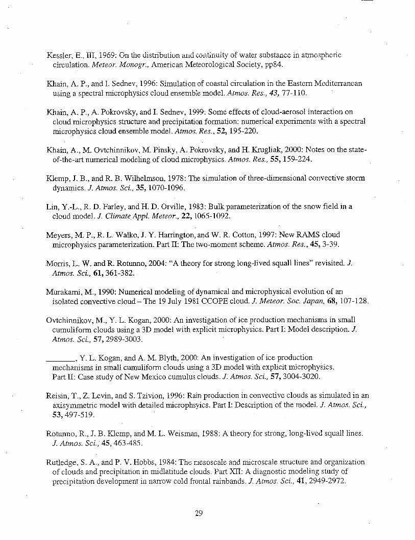
4 n i n Kessier, E., III, iyoy: On iiie dis’diuiiun arid ioiitiniiity of W Z k i siibstziize in atmzlspheric circulation. Meteor. Monogr., American Meteorological Society, pp84.

Khain, A. P., and I. Sednev, 1996: Simulation of coastal circulation in the Eastern Mediterranean using a spectral microphysics cloud ensemble model. Atmos: Res., 43, 77-1 10.

Khain, A. P., A. Pokrovsky, and I. Sednev, 1999: Some effects of cloud-aerosol interaction on cloud microphysics structure and precipitation formation: numerical experiments with a spectral microphysics cloud ensemble model. Atmos. Res., 52, 195-220.

Khain, A., M. Ovtchinnikov, M. Pinsky, A. Pokrovsky, and H. Krugliak, 2000: Notes on the state- of-the-art numerical modeling of cloud microphysics. Atmos. Res., 55,159-224.

Klemp, J. B., and R. B. Wilhelmson, 1978: The simulation of three-dimensional convective storm dynamics. J. Atmos. Sci., 35, 1070-1096.

Lin, Y.-L., R. D. Farley, and H. D. Orville, 1983: Bulk parameterization of the snow field in a cloud model. J. Climate Appl. Meteor., 22,1065-1092.

Meyers, M. P., R. L. Walko, J. Y. Harrington, and W. R. Cotton, 1997: New RAMS cloud microphysics parameterization. Part II: The two-moment scheme. Atmos. Res. , 45,3-39.

.Morris, L. W. and R. Rotunno, 2004: “A theory for strong long-lived squall lines” revisited. J. Atmos. Sci., 61,361-382.

Murakami, M., 1990: Numerical modeling of dynamical and microphysical evolution of an isolated convective cloud - The 19 July 1981 CCOPE cloud. J. Meteor. SOC. Japan, 68, 107-128.

Ovtchinnikov, M., Y. L. Kogan, 2000: An investigation of ice production mechanisms in small cumuliform clouds using a 3D model with explicit microphysics. Part I: Model description. J. Atmos. Sci., 57,2989-3003.

, Y. L. Kogan, and A. M. Blyth, 2000: An investigation of ice production mechanisms in small cumuliform clouds using a 3D model with explicit microphysics. Part 11: Case study of New Mexico cumulus clouds. J. Atmos. Sci., 57,3004-3020.

Reisin, T., Z. Levin, and S. Tzivion, 1996: Rain production in convective clouds as simulated in an axisymmetric model with detailed microphsyics. Part I: Description of the model. J. Atmos. Sci., 53,497-519.

Rotunno, R., J. B. Klemp, and M. L. Weisman, 1988: A theory for strong, long-lived squall lines. J. Atmos. Sci., 45,463-485.

Rutledge, S. A., and P. V. Hobbs, 1984: The mesoscale and microscale structure and organization of clouds and precipitation in midlatitude clouds. Part XTI: A diagnostic modeling study of precipitation development in narrow cold frontal rainbands. J. Atmos. Sci., 41,2949-2972.

29

Rutledge, S. A., R. A. Houze, Jr., and M. I. Biggerstaff, 1988: The Olkahoma-Kansas mesoscale convective system of 10- 11 June 1985: Precipitation structure and single-doppler radar analysis. Mon. Wea. Rev., 116,1409-1430.

Rutledge, S. A., and D. R. MacGoman, 1988: Cloud-to ground lightening activity in the 10-11 June 1985 mesoscale convective system observed during the Oklahoma-Kansas PRE-STORM project. Mon. Wea. Rev., 116, 1393-1408.

Shiino, J., 1983: Evolution of raindrops in an axisymmetric cumulus model. Part I. Comparison of the parameterized with non-parameterized microphysics. J. Meteor. SOC. Japan, 61,629-655.

Smolarkiewicz, P. K., and W. W. Grabowski, 1990: The multidimensional positive advection transport algorithm: nonoscillatory option. J. Comput. Phys., 86,355-375.

Smull, B. F., and R. A. Houze, Jr., 1987a: Dual-Doppler radar analysis of a midlatitude squall line with a trailing region of stratiform rain. J. Atmos. Sci., 44,2128-2147.

Smull, B. F., and R. A. Houze, Jr., 1987b: Rear inflow in squall lines with trailing stratiform precipitation. Mon. Wea. Rev., 115,2869-2889.

Soong, S., 1974: Numerical simulation of warm rain developmentin an axisymmetric cloud model. J: Atmos. Sci., 31, 1262-1285.

Takahashi, T., 1975: Tropical showers in an axisymmetric cloud model. J. Atmos. Sci., 32, 1318- 1330.

Tao, W.-K. and J. Simpson, 1993a: Goddard Cumulus Ensemble Model. Part I: Model description. Terr. Atmos. Oceanic Sci., 4,35-72.

, J. Simpson, C.-H. Sui, B. Femer, S. Lang, J. Scala, M.-D. Chou, and K. Pickering, 1993b: Heating, moisture, and water budgets of tropical and midlatitude squall lines: Comparisons and sensitivity to longwave radiation. J. Atmos. Sci., 50,673-690.

.

, S. Lang, J. Simpson, C.-H. Sui, B. Femer, and M.-D. Chou, 1996: Mechanisms 0-f cloud-radiation interaction in the tropics and midlatitudes. J. Atmos. Sci., 53,2624-2651.

, J. Simpson, D. Baker, S. Braun, M.-D. Chou, B. Femer, D. Johnson, A. Khain, S. Lang, B. Lynn, C.-L. Shie, D. Stan-, C.-H. Sui, Y. Wang, and P. Wetzel, 2003: Microphysics, radiation and surface processes in the Goddard Cumulus Ensemble (GCE) model. Meteorol. Amos. Phys., 82,97-137,2003.

Wang, C., and J. S. Chang, 1993: A three-dimensional numerical model of cloud dynamics, microphysics, and chemistry, 1 , Concepts and formulation, J. Geo. Res., 98@8), 14827-14844.

30

Willis, P. T. and A. J. Heymsfield, 1989: Structure of the melting layer in mesoscale convective system stratiform precipitation. J. Atmos. Sci., 46, 2008-2025.

Yin, Y., 2. Levin, T. G. Reisin, and S. Tzivion, 2000a: Seeding convective clouds with hygroscopic flares: Numerical simulations using a cloud model with detailed microphysics. J. Appl. Meteorol., 39, 1460-1472.

-, --y -, and ---, 2000b: The effects of giant cloud condensation nuclei on the development of precipitation in convective clouds-A numerical study. Atmos. Res., 53,9 1-1 16.

Zhang, D.-L., and K. Gao, 1989: Numerical simulation of an intense squall line during 10-1 1 June . 1985 PRE-STORM. Part II: Rear inflow, surface pressure perturbations and stratiform

precipitation. Mon. Wea. Rev., 117,2067-2094.

31

Figure Captions:

Figure 1: Radar reflectivity after 12 hours of simulation for the bulk (la) and bin (lb) schemes.

Figure 2: Radar reflectivity and horizontal relative flow in m s-' observed at 0345 UTC in the

June 10-1 1 PRE-STORM case. Copied from fig. 5 in Rutledge et al. (1988).

Figure 3: Time series of 30 dBZ radar echo top of the leading convective cell in the bulk (solid

line) and bin (dashed line) simulations.

Figure 4: Time-domain diagram of surface rainfall for the bulk (4a) and bin (4b) schemes.

Figure 5: Time series of the domain average surface rainfall rate for the bulk (black lines) and

bin (gray lines) simulations. The upper two lines are total surface rainfall rate, and lower two

lines are stratiform rainrate using the CH-84 separation method.

Figure 6: Surface rainfall amount probability density plot for the June 10-11 PRE-STORM case.

Figure 7: Horizontal wind field at the end of the simulation (12 hours) for the bulk (7a) and bin

(7b) scheme. Contour levels are -15, 10, -5,0, 5, 10, and 15m s-', with negative contours shown

in dashed lines.

Figure 8: Vertical air velocity field after 12 hours of simulation for the bulk (8a) and bin (8b)

scheme. Contour levels are -5, -1, -0.5, -0.1, 0.1, 1, 5 , 10, and 20 m s-', with negative contours

shown in dashed lines. Updraft cores with w bigger than 1 m s-' are darkly shaded. Downdraft

cores with w less than -1 m s-' are lightly shaded.

Figure 9: Time series of maximum and minimum vertical air velocity (m s-') for both the bulk

(solid lines) and bin (dotted lines) simulations. Negative values represent downdrafts. The

minimum velocity is calculated using only data below 5 km.

Figure 10: Average vertical air velocity profiles for the stratiform region 12 hours into the

simulation. The dotted line is for the bin simulation averaged between x=130 km and 180 km in

fig. 8b. The dashed line is for the bulk simulation averaged between x=150 km and 190 km in

fig. 8a; The dashed-dot line is for the bulk simulation averaged between x=150 km and 210 km

in fig. 8a. Thin solid lines are from EVAD calculations of the same case using CP3 and CP4

radar (Rutledge et al. 1988), and the thick solid line is the dual doppler radar estimation

(Biggerstaff and Houze 1993).

Figure 11: Pressure perturbations in mb for both the bulk and bin simulations. Positivehegative

values are in soliddashed lines. The contour intervals are 0.5 mb.

32

Figure 12: Eoteniiai ierlipei-atuie pe&~bsiioii fields ~t t=!2 ~ G X S f i r thz bulk (122) 2nd bin

(12b) models. Contour levels are -5 4, -3, -2, -1, 0,2,4, 6 K, with negative contours in dashed

lines. -3 K lines are marked with thick dashed lines.

Figure 13: Condensatiodevaporation rate field in g g-' day-' for the buik (13a) and bin (13b)

simulations. Positive values (condensation) are in solid lines, and negative values (evaporation)

are in dashed lines. Contour levels are -0.2, -0.1, -0.05, -0.01,0.01,0.05,0.1, 1.0 g g-' day-'.

Areas with evaporation rates stronger than -0.1 g g-' day-' are shaded in gray.

Figure 14: Time series of the maximum evaporation rate in g g-' day-'. Only,evaporation rates

below the melting level are used. The solid (dashed) line is the bulk (bin) simulation.

33

Table Captions:

Table 1: Stratiform rain percentage for the June 10-11 PRESTORM case.

Table 2: Updraft core statistics for the PRE-STORM case.

lL

Table 1: Stratiform rain percentage for the June 10-1 1 PRE-STORM case.

Table 2: Updraft core statistics for the PRE-STORM case. -

34

z o : ' ' ( a ) ' ' ' ' I " ' " " ' ' I ' . " i '

15 - - - -

E 5 10 I\.

5

0 0 50 200 250

PREST.ORM BIN Reflectivity (dBZ) - - - -

15

E 5 10 N

5

0 100 150 200 2 50 n 50

50 40

30 20 10 0

Figure 1: Radar reflectivity after 12 hours of simulation for the bulk (la) and bin (lb) schemes.

35

1 l-&JN-85 CP4 RHI 03~45 Z 12 4

109

S A

7 9

6.4

4.9

3.4

1.9

k

12.4

109

9.4

79

6 4

4 9

34

1 9

4

Distance from Radar (Km)

Figure 2: Radar reflectivity and horizontal relative flow in m s-’ observed at 0345 UTC in the

June 10-1 1 PRE-STORM case. Copied from fig. 5 in Rutledge et al. (1988).

36

n

Y E W

Q 0

0 1 0 0

U -0

4-J

L

E

14

12

10

8

6

4

2

0 0

I I I

Bulk

. ............ Bin

I I I

200 400 time (min)

600

Figure 3: Time series of 30 dBZ radar echo top of the leading convective cell in the bulk (solid

line) and bin (dashed line) simulations.

37

Y E. R P, c-.l c-.l

n c 0- W

0

< 0

A

P 0

h

N

- 0

5- v

A

h,

0 m

(A 0 0

N 0 0

time (min) P 0 0

0, 0 0

m Z

cn 0 I n

N Ln 0 0 2 Ln 0 0 0

38

bin (gray lines) simulations. The upper two lines are total surface rainfall rate, and lower two

lines are stratiform rainrate using the CH-84 separation method.

39

20

15

10

5

C

. . \ ..

0 10 20 ‘30 40 50 60 70 80 90 100110120 rainiate (mm/hr)

Figure 6: Surface rainfall amount probability density plot for the June 10-1 1 PRE-STORM case.

40

-

- -

15 -

-... ...........................-5. Q ................. .................. ,--. ....................................................... ........................... E

10 _. - ....................................... - N

150 200 250 0 50 100

Bin u (m/s)

n 15

A C 8 5 10

0

.................................................... ......... ............ ............................................................

I

Figure 7: Horizontal wind field at the end of the simulation (12 hours) for bulk (7a) and bin (7b)

scheme. Contour levels are -15, 10, -5, 0,5, 10, 15m s-*, with negative contours shown in dashed

lines.

41

F-.

E Y v

N

20

15

10

5

0 0 50 200 250

A

E Y

N

v

\ , I

0 50 200 2 50

Figure 8: Vertical air velocity field after 12 hours of simulation for the bulk (8a) and bin (8b)

scheme. Contour levels are -5, -1, -0.5, -0.1, 0.1, 1, 5 , 10, and 20 m s-', with negative contours

shown in dashed lines. Updraft cores with w bigger than 1 m s-' are darkly shaded. Downdraft

cores with w less than -1 m s-l are lightly shaded.

42

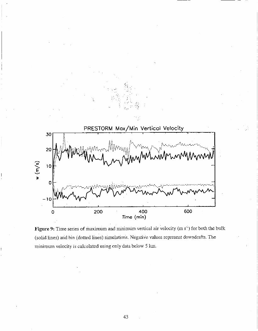
Figure 9: Time series of maximum and minimum vertical air velocity (m s-') for both the bulk

(solid lines) and bin (dotted lines) simulations. Negative values represent downdrafts. The

minimum velocity is calculated using only data below 5 km.

43

15

- 10 E Y . W

5

0 -1.0 -0.8 -0.6 -0.4 -0.2 0.0 0.2 0.4 0.6 0.8 1.0

w ( 4 4

Figure 10: Average vertical air velocity profiles for the stratiform region 12 hours into the

simulation. The dotted line is for the bin simulation averaged between x=130 km and 180 km in

fig. 8b. The dashed line is for the bulk simulation averaged between x=150 km and 190 km in

fig. 8a; The dashed-dot line is for the bulk simulation averaged between x=l50 km and 210 kni

in fig. 8a. Thin solid lines are from EVAD calculations of the same case using CP3 and CP4

radar (Rutledge et al. 1988), and the thick solid line is the dual doppler radar estimation

(Biggerstaff and Houze 1993).

44

(a) Bulk AP (mb)

- .. . . - - .-- . - . . . . . . .o ... - ................................. ......'< * . . . . . . f . ....

- .......... .................. ....... .'-3.0 -..:. ..... ,. ..... %,

. - . . - . . . . . . . . . . . . - . . . . . -

. -. - ......... ....... ..... . . . . . . . -2.5 ...: ._ ..-.. ._ . . - .- .............. . . . . . . . . -

- ............ . * . ...... 7 .... .................. . . . . . . . . ............. ... - . . . . . . . . . ....... ,2.5

...... __-.- -

. . . . . .. . . . . . . . . . . . . - 7..

..... . . . ..

A

E Y v

N

20

15

0

5

0 0

20

1'5

,--. E 5 10 N

5

0

50 100 150 x (km)

(b ) Bin AP (mb)

200 250

................................................... - ........ ....... - - - - - ......... ,,5 - -

.............. .----.

--._ -. .-1.0.

. . .

r....-1,0

.. ........................................ .....-,. 5 . . . . . . . . . . . . . . .

2.0 ...................................................... _ _ . _ I . _ . _ . _ _ _ . _ _ _ . _ . _ . _ _ _ _ . _ _ _ _ _ _ . _ - ................ - .... . ................. - - .... ..... : a

* ..- .. I -.-1.5

-2 .5 . - . - - .

..... -2.0 ....................................... s ............ -2.0 . . . . . . . . . . . . . . .................... . . . . . . . . . . ....... ................ ...................................................... .....- 1. 5 . ....................... ;:.-.:. .. .. : ._ ~, , , , I I :I .... .................................................... . . - .............. ( . . .. /J . . . . . . . . . . - 0 ............ .I. ..................... .I. .....

0 50 200 250

Figure 11: Pressure perturbations in the unit of mb for both bulk and bin simulations.

Positivehegative values are in soliddashed lines. The interval of the contours is 0.5 mb.

45

1

1 - E Y

N

v

(a) Bulk A€J (K)

L

(b) Bin Ae (K) . . . -

100 150 200 250 100 150 200 250 x (km) x (km)

Figure 12: Potential temperature perturbation fields at t=12 hours for the bulk (12a) and bin

(12b) models. Contour levels are -5 4, -3, -2, - 1 , O , 2,4, 6 K, with negative contours in dashed

lines. -3 K lines are marked with thick dashed lines.

46

Bulk Cond/Evap Rate Bin Cond /Evap Rate

10 ,-. , , E

Y

N

v

5

0 100 150 200 250 100 150 200 250

x (km) x (km)

Figure 13: Condensatiodevaporation rate field in g g-' day-' for the bulk (13a) and bin (13b)

simulations. Positive values (condensation) are in solid lines, and negative values (evaporation)

are in dashed lines. Contour levels are -0.2, -0.1, -0.05, -0.01, 0.01,0.05, 0.1, 1 .O g g-' day-'.

Areas with evaporation rates stronger than -0.1 g g-' day-' are shaded in gray.

47

0.0 I I I I

1. . ..

-0.5

- 1 .o

, . * . - I .. . ..

: .. . ~ . ,. . * .' . . . . .. ... . . e . . ;

: *. . : '. * . . . .

BULK ____~. . ._ .__ BIN

Figure 14: Time series of the maximum evaporation rate in g g-' day-'. Only ,evaporation rates

below melting the level are used. The solid (dashed) line is the bulk (bin) simulation.

48

Popular Summary Submitted as an article to Journal of the Atmospheric Sciences, June 2004.

Title: Sensitivity of a Cloud-Resolving Model to the Bulk and Explicit Bin Microphysical Schemes. Part I: Validations with a PRE-STORM Case

Authors: Xiaowen Li', Wei-Kuo Tao2, Alexander P. main3, Joanne Simpson', and Daniel E. Johnson'

The Goddard Cumulus Ensemble Model (GCE) is used to study sensitivities of two different microphysical schemes, one is the bulk type, and the other is an explicit bin scheme, in simulating a mid-latitude squall line case (PRE-STORM, June 10-1 1, 1985). Simulations using dlfferent microphysical schemes are compared with each other and also with the observations. Both the bulk and bin models reproduce the general features during the developing and mature stage of the system. The leading convective zone, the trailing stratiform region, the horizontal wind flow patterns, pressure perturbation associated with the storm dynamics, and the cool pool in front of the system all agree well with the observations. Both the observations and the bulk scheme simulation serve as validations for the newly incorporated bin scheme. However, it is also shown that the bulk and bin simulations have distinct differences, most 'notably in the stratiform region. Weak convective cells exist in the stratiform region in the bulk simulation, but not in the bin simulation. These weak convective cells in the stratiform region are remnants of the previous stronger convections at the leading edge of the system. The bin simulation, on the other hand, has a horizontally homogeneous stratiform cloud structure, which agrees better with the observations. Preliminary examinations of the downdraft core strength, the potential temperature perturbation, and the evaporative cooling rate show that the differences between the bulk and bin models are due mainly to the stronger low-level evaporative cooling in convective zone simulated in the bulk model.

' Goddard Earth Science and Technology Center, University of Maryland, Baltimore County 2Laboratory for Atmosphere, NASA Goddard Space Flight Center 'The Hebrew University of Jerusalem, Jerusalem, Israel