Embed Size (px)
Citation preview
University of Alberta
Characteristics of the Vortex Structure in the Outlet of a
Stairmand Cyclone: Regular Frequencies and Reverse Flow
Mei Chen O
A thesis submitted to the Faculty of Graduate Studies and Research in partial fulfillment
of the requirernents for the degree of Master of Science in Chemical Engineering
Department of Chemical and Materials Engineering
Edmonton, Alberta
FaIl 1999

National Library I*$1I of Canada Bibliothèque nationale du Canada
Acquisitions and Acquisitions et Bibliographie Services senrices bibliographiques
395 Wellington Street 395. rue Wellington OttawaON K1AON4 OttawaON K1AON4 Canada Canada
The author has granted a non- exclusive licence allowing the National Library of Canada to reproduce, Loan, distribute or sel1 copies of this thesis in rnicrofom, paper or electronic formats.
The author retains ownershp of the copyright in this thesis. Neither the thesis nor substantial extracts fiom it may be printed or othenvise reproduced without the author's permission.
L'auteur a accordé une licence non exclusive permettant a la Bibliothèque nationale du Canada de reproduire, prêter, distribuer ou vendre des copies de cette thèse sous la forme de microfiche/filrn, de reproduction sur papier ou sur format électronique.
L'auteur conserve la propriété du droit d'auteur qui protège cette thèse. Ni la thèse ni des extraits substantiels de celle-ci ne doivent être imprimés ou autrement reproduits sans son autorisation.

To my diligent and sacri ficial parents
To whom 1 owe al1 that I am
Abstract
In this project. a combination of experiments and simulations is used to investigate the
penetration of the processing vortex core into the cyclone, the extent of the reverse flow,
and the impact of the geometry on the flow field.
Periodic motions were detected in the gas outlet tube or just outside of the gas outlet tube
with the three gas outlet tube diameters tested. The observed oscillations are caused by a
coherent structure. These oscillations grow less vigorous down the gas outlet tube and
eventually die out. Time avenged axial velocity profiles at different elevations indicate
that the back flow region shrinks down the gas outlet tube.
Numerical simulation (3D) was also conducted. With the Reynolds Stress Mode1 (RSM)
to account for the non-isotropie effect of turbulence in the highly swirling tlow, the CFD
simulation prove to be effective in capturing the essential features of the flow in cyclone.

Acknowledgments
1 must begin by acknowledging Professor Kresta and Professor Mees, who were
excellent instructors, motivators and overseers of the project. In addition, ail my
colleagues in our group gave me much help. Dr. Bara and Dr. Hackman at Syncmde
Canada are thanked for their much insightful advice.
To the list 1 must add the personnel in the machine shop. DACS center and the
instrument shop. for their hard work.
The financial aid for this project was graciously provided by Syncmde Canada
Ltd.
Table of Contents
Chapter 1 : Introduction ............................................................................... 1 1 . 1 The fùnction of a cyclone ...................................................................... 1
.......................................................... 1.2 Geometric variables of a cyclone 1
....................................................... 1.3 General flow pattern in a cyclone 1 7 ................................................... 1.4 The mechanism of particle separation , . . .......................................................................... 1.5 Previous investigattons 3
........................................................................... . 1 .5 1 Experimental work 3 ...... .................................. . 1 .5 1.1 Back flow in the center of the core ., 3
........................................................... . 1 .5 1.2 Flow oscillation in cyclone 5 ............................................................................... 1 S.2 Numerical work 8
................................................................. 1.6 Approach used in this work 10
Chapter 2: Experimental ............................................................................ 17 2.1 The principle of laser Doppler anemometry (LDA) - an overview .... 17 2.2 Optical system .................................................................................... 19
2.2.1 Optical configurations ................................................................... 19 2.2.2 Optical requirements and cornponent measured in the study ........ 20
2.3 Seeding design (seeding tank) ............................................................ 21 .................................................................. 2.4 Cyclone mode1 and blower 24
2.4.1 Cyclone mode1 .................................... .... ................................ 24 2.4.2 Blower ............................................................................................ 25
2.5 Cyclone alignment .............................................................................. 26 2.6 Experiment error prediction and equipment calibration ..................... 27 2.7 Conclusion ........................................................................................... 28 Reference .................................................................................................. 3 8

............................................................... Chapter 3: Experimental results 39 3.1 Data analysis technique ................................................................ 39
........................................................................ 3.1.1 Alias fiee sampling 39 3.1.2 Turbulence power spectrum ......................................................... 40 3.1.3 Transformation to fiequency domain using FFT ........................... 40
............................................................... 3.1.4 Autocorrelation Function 42 3.1.5 Analyzing unevenly spaced data ................................................. 42
.................................................................. 3.2 Flow field rneasurements 44 ................................................................................... 3.2.1 Inlet velocity 44
3.2.2 Axial velocity ................................................................................. 45 ..................................................................... 3.2.3 Tangential velocity 49
..................................... 3.2.4 Measurements at different inlet velocities 51 3.2.5 Measurements at different gas outlet tube diameters ..................... 51
............................................................................................ 3.3 Discussion 52 ......................................................... 3.3.1 The mechanisrn of back flow 52
............... 3.3.2 Origin of coherent stmcture and asymmetric flow tiled 54 ..................................................................... 3.3.3 Volumetric flow rate 54
3.3.4 Momentum balance ....................................................................... 55 3.4 Conclusions .......................................................................................... 56 Re ferences : ................................................................................................. 88
Chapter 4 Characterization of swirling flows in cyclone using ................................................................................... dimensional analysis 90
4.1 Dimensional anal y sis. .................................................................... 90 . . 4.1.1 Buckingham s Pi theorern ............................................................ 90
4.1.2 Nondimensional parameter determined fiom differential equations . ............................................................................................................... 92
........................................................................................ 4.2 Swirl number 94 .................... 4.2.1 Generation of swirl and calculation of swirl number 97
................................................................................... 4.3 Strouhal number 97 ........................... ..........*.....................................-.........*......*.. 4.4 Results ... 99
Reference: ................................................................................................ 1 03
Chapter 5: Computational Techniques ................................................ 1 5.1 Introduction ........................................................................... 1 04 5.2 Computational Fluid Dynamics Soiver FLUENT .......................... 1 04
5.2.1 Mathematical Formulation .................................................... 1 04 5.2.2 Turbulence Models ............................................................... 1 06 5.2.3 Computational domain. boundary conditions and time step .... 1 08
5.2 Validation of CFD results ......................................................... 1 1 1 5.3 Numerical results versus experirnental results ............................... 1 12 5.4 Prediction of the frequency of oscillation ................................... 1 13
5.4.1 Tirne averaged velocity prediction ........................... ... ........... 1 14 . . . 5.4.2 Solution sensitivity .................................................................... 1 15
5.5 Possible reasons for the discrepancy between experiment and simulation ...................................................................................... 1 15
................................................................................... 5.6 Conclusion: 1 17
Chapter 6: Conclusions ....................................................................... 133
List of Tables
Table Page
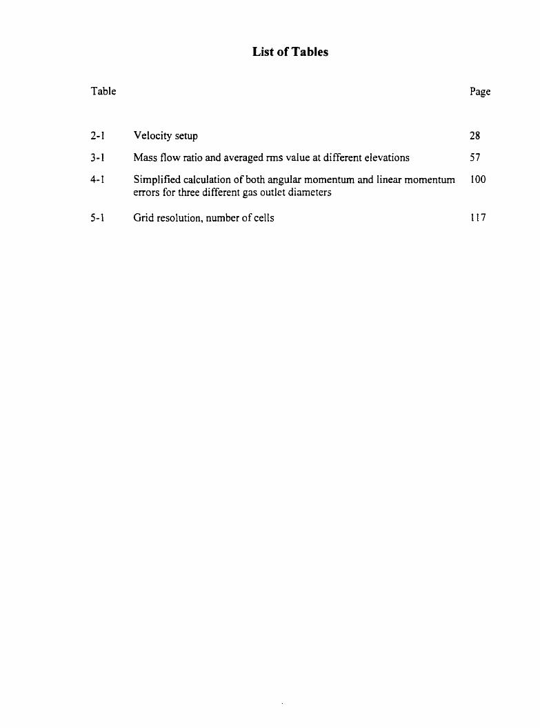
2- 1 Velocity setup 28
3-1 Mass flow ratio and averaged rms value at different eirvations 57
4- 1 Simplified calculation of both angular momentum and iinear momenturn 100 errors for three different gas outlet diameters
5-1 Grid resolution, number of celIs 117

List of Figures
Cyclone geometry and generai flow pattern
Cross-sectionai dimensions of a reverse flow cyclone
Fractional separation efficiency
Schematic diagrarn of expenmental setup (dimensions are in meters)
LDA rneasuring volume as envision by the fnnge interpretation (fiorn George, 1 988) Schematic o f the Aerometrics LDA optical configuration
Beam orientation
A: Measurement of tangential velocity
B: Measurernent of radial velocity
Refraction of laser Doppler anemometer beams during measurement of radial velocity (Broadway & Karahan. 1 98 1 ) Deviation angle in the cone of cyclone when rneasuring radial velocity at z=300 mm from the bottorn Diagram of dry ice tank
Cyclone mode1 in lab (dimensions arc in meters)
The connection of cyclone inlrt to hose
Repeatability and calibration of the inlet velocity
Inlet velocity distribution at motor load=90%
Cyclone supports and traverses
Tangential velocity measurernents with varying sarnple size
Measurement position in experiments
Repeatability and calibration of inlet velocity for different diameter of gas outlet tube Inlet tangential velocity profile at 100% motor load
Inlet superficial velocity at three different gas outiet tube diameters
Time series of tangentid velocity in cyclone inlet at x/a=0.33 and y/b=0.4
Frequency analysis in cyclone inlet at x/a=0.33 and yb=0.4
Autocorrelation coefficient in cyclone inlet at x/a=0.33 and y/b=0.40
Time series of axial velocity in cyclone outlet at htop=50 mm and ~ 3 2 . 5 mm Frequency analysis in cyclone outlet at htOp=50 mm and ~ 3 2 . 5 mm
Autocorrelation coefficient in cyclone outlet at htOp=50 mm and 4 2 . 5 mm
Frequency analysis at the top of cyclone outlet at htop=-2 mm and ~ 3 0 mm
Frequency analysis at the top of cyclone outlet at htop=2 mm and r=20 mm
Frequency analysis at the top of cyclone outlet at htop=-2 mm and r=10 mm
Time series of axial velocity at the top of cyclone outlet at htOp=-13 mm and
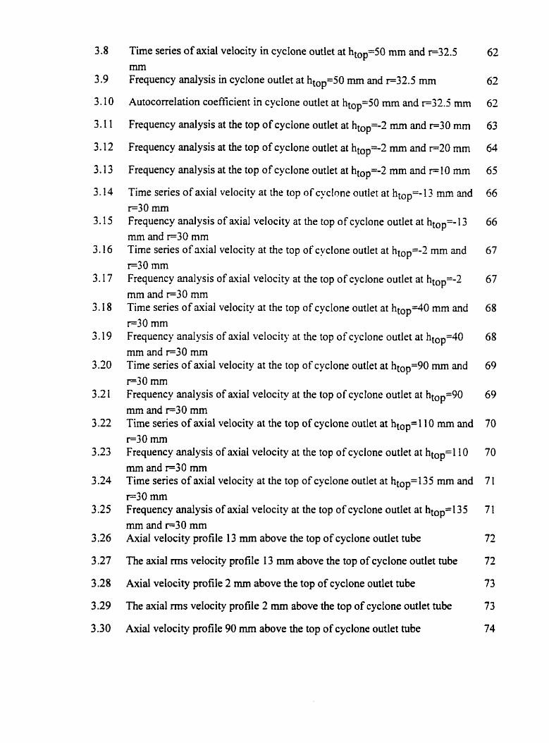
r=30 mm Frequency analysis of axial velocity at the top of cyclone outlet at htop=-l 3 mm and r=30 mm Time senes of llvial velocity at the top of cyclone outlet at htop=-2 mm and r-30 mm Frequency analysis of axial velocity at the top of cyclone outlet at htop=-2 mm and r-30 mm Time series of axial velocity ai the top of cyclone outlet at htop=40 mm and
r=30 mm Frequency analysis of axial velocit) at the top of cyclone outlet at htop=40 mm and r=30 mm Time series of axial velocity at the top of cyclone outlet at htop=90 mm and r=30 mm Frequency analysis of axial velocity at the top of cyclone outlet at htop=90 mm and i-30 mm Time senes of axial velocity at the top of cyclone outlet at htop=l 10 mm and r=30 mm Frequency analysis of axial velocity at the top of cyclone outlet at htop=l 10 mm and r-30 mm Time series of axial velocity at the top of cyclone outlet at htop=l 35 mm and r=30 mm Frequency analysis of axial velocity at the top of cyclone outlet at hmp=i 35 mm and r=30 mm Axial velocity profile 13 mm above the top of cyclone outlet tube
The axial mis velocity profile 13 mm above the top of cyclone outlet tube
Axial velocity profile 2 mm above the top of cyclone outlet tube
The axial mis velocity profile 2 mm above the top of cyclone outlet tube
Axial velocity profile 90 mm above the top of cyclone outlet tube 74
The axial rms velocity profile 90 mm above the top of cyclone outlet tube
Axial velocity profile 135 mm above the top of cyclone outlet tube
The axial rms velocity profile 135 mm above the top of cyclone outlet tube
Tangential velocity profile in the barrel at htop=41 5 mm
Tirne senes of tangential velocity at the top of cyclone outlet at htop=- I mm and r=27.5 mm Frequency analysis at the top of cyclone outlet at htOp=-1 mm and ~ 2 7 . 5 mm Autocorrelation coefficient at the top of cyclone outlet at htOp=-1 mm and r=27.5 mm Time series of tangential velocity at the top of cyclone outlet at htop=41 5 mm and r=30 mm Frequency analysis at the top of cyclone outlet at htop-a 4 1 5 mm and r=20
mm Autocorrelation coefficient at the top of cyclone outlet at htop=415 mm and ~ 2 0 mm Frequency analysis in cyclone barre1 at htop=4 15 mm and r 4 O mm
Frequency analysis in cyclone barrel at htOp=380 mm and r=40 mm
Frequency analysis in cyclone cone at htop=770 mm and r=25 mm
Autoco~elation coefficient in cyclone cone at htOp=770 mm and r=25 mm
Time series of axial velocity at the top of cyclone outlet at htop=50 mm and r=20 mm, at 50% motor load Frequency analysis at the top of cyclone outlet at htop=50 mm and r=20 mm. at 50% motor Ioad Autocorrelation coefficient at the top of cyclone outlet at htop=50 mm and r=20 mm, at 50% rnotor load Oscillation frequency in the gas outlet tube
Frequency analysis just outside of gas outlet tube at htop=- 1 mm and r=20 mm Axial velocity profile 2 mm above the top of cyclone outlet tube (with Doutlet/Dbarrel=0*33) The axial rms velocity profile 2 mm above the top of cyclone outlet tube (with Do u t le t/D barre 1'0.33 Frequency analysis in cyclone outlet at htOp=1 60 mm and r=35 mm
Axial velocity profile 2 mm above the top of cyclone outlet tube (with

The axial rms veiocity profile 2 mm above the top of cyclone outlet tube 87 (with Doutletmbarrel'0-63) Frequency parameter as a function of Reynolds number 1 O 1
Frequency swirl ratio as a h c t i o n of Reynolds nurnber 102
Schematic representation of a typical2D-computattional cell surroundhg 118 code np Cyclone mode1 in simulation 119
Overview of the numerical solution process 120
Velocity vector in barrel at ~ 0 . 4 0 1 m when V;,=?6.667 mls
Cornparison of tangential velocity profile at the top of the cyclone outlet tube 121
Velocity vector of axial and radial velocity at x=O cross section of z=O.X to 123 ~ 0 . 3 9 Oscillation predicted by simulation at a point at ~ 0 . 6 5 m and ~ 5 m m 124
Frequency change with time in numerical simulation 125
Oscillation damping predicted by numerical simulation in cyclone barrel at 136 ~ 0 . 5 rn and r=O mm Oscillation damping predicted by numerical simulation in cyclone cone at 126 z=0.3 m and r =5 mm Axial velocity contour on the xz plane 127
Axial velocity profile 90 mm from the top of cyclone outlet tube 128
Axial rms velocity profile 90 mm from the top of cyclone outlet tube 138
Axial velocity profile in the gas outlet tube 135 mm fiom the top of the 129 cyclone outlet tube Axial rms velocity in the gas outlet tube 135 mm from the top of cyclone 129 outlet tube Refined grid 130
Time step sensitivity of axial velocity test at z=0.7 rn 131
Nomenclature
inlet width
inlet area
inlet hight
barre1 diameter
gas outlet tube diameter
critical size particle diameter
one dimensional power s p e c t m
oscillation frequency
centrifuga1 force
Doppler frequency
drag force
axial flux of swirl momentum
aviai flux of axial momentum
continuous fourier transform
continuous time series of data
complex conjugate
discrete fourier transform
discrete time series data
height with respect to the top of cyclone
friction loss coefficient at the inlet
friction loss coefficient in the outlet tube
axial momentum
N yquist fiequenc y
pressure
volwnetric flow rate
m
m2
m
m
m
FLm
rn2is
1 /s
N
MHz
N
kg rn'/s2
rn/s
m/s
mis
mls
m/s
m
radial position
Reynolds number
autocorrelation coefficient function
the Strouhal number
the Swirl nurnber
time lag
axial velocity
tangential velocity
fluctuating velocity
fluctuating velocity contributed by periodic motion turbulence fluctuating velocity
radial velocity
tangential velocity
Greek
axial direction
time
beam intersection angle
viscosity of gas
angular velocity
wavelength of light
fringe spacing
vorticity at r direction
S
rad
kgim s
rad/s
m
Pm
1 /s
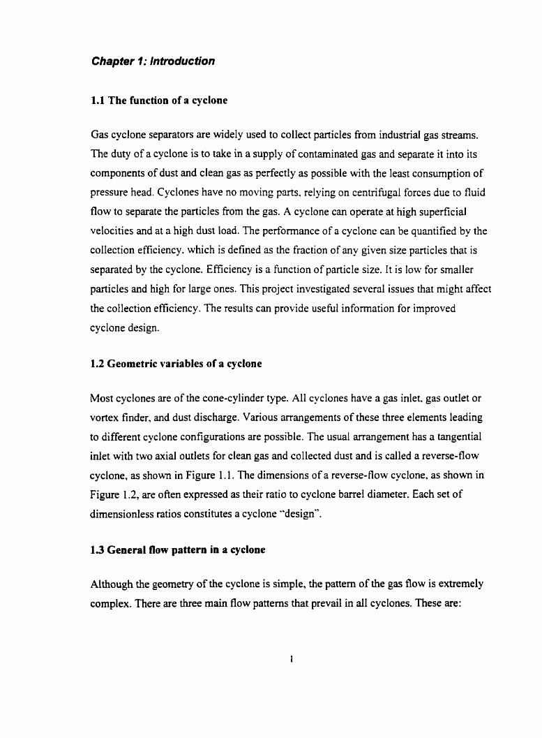
1.1 The function of a cyclone
Gas cyclone separatoe are widely used to collect particles fiorn industrial gas streams.
The duty of a cyclone is to take in a supply of contaminated gas and separate it into its
components of dust and clean gas as perfectly as possible with the least consurnption of
pressure head. Cyclones have no moving parts. relying on centrifuga1 forces due to fluid
flow to separate the particles fiom the $as. A cyclone can operate at high superficial
velocities and at a high dust load. The performance of a cyclone can be quantified by the
collection efficiency. which is defined as the fraction of any given size particles that is
separated by the cyclone. Efficiency is a function of particle size. It is low for smaller
particles and high for large ones. This project investigated several issues that might affect
the collection efficiency. The results c m provide usefül information for improved
cyclone design.
1.2 Geometric variables of a cyclone
Most cyclones are of the cone-cylinder type. AI1 cyclones have a gas inlet. gas outlet or
vortex finder, and dust discharge. Various arrangements of these three elements leading
to different cyclone configurations are possible. The usual arrangement has a tangential
inlet with two axial outlets for clean gas and collected dust and is cdled a reverse-flow
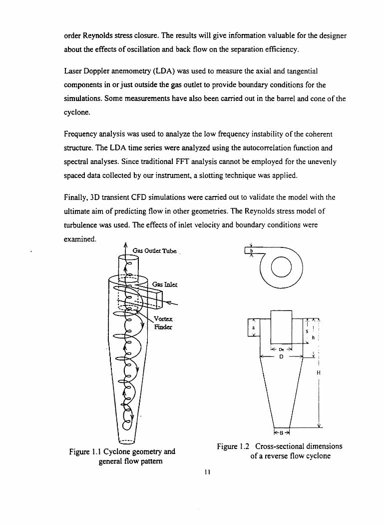
cyclone, as shown in Figure 1.1. The dimensions of a reverse-flow cyclone, as shown in
Figure 1.2, are ofien expressed as their ratio to cyclone barre1 diameter. Each set of
dirnensionless ratios constitutes a cyclone "design".
1.3 General flow pattern in a cyclone
Although the geometry of the cyclone is simple, the pattern of the gas flow is extremely
cornplex. There are three main flow patterns that prevail in al1 cyclones. These are:

Descending spiral flow - This pattern canies the separated dust down the wails of the
cyclone.
Ascending spiral flow - This rotates in the same direction as the descending spiral.
but the cleaned gas is carried from the dust discharge to the gas outlet.
Radially inward flow - This feeds the gas from the descending to the ascending spiral.
Cyclone performance is evaluated in tems of pressure drop and collection efficiency. To
assess factors that contribute to performance, the tangential, radial. and axial velocity
components of the velocity field must be understood. The axial velocity is directed
upwards in the core and downwards along the wall. The absolute value of the radial
velocity is at least one order of magnitude lower than the axial velocity components. Its
magnitude is probably as large as the fluctuation of the tangential and mial velocity
cornponents. The tangential velocity c m be described as a Rankine vortex. i.e. a
combination of a free vortex and a forced vortex. The tangential velocity increases with
the radius and reaches a maximum at about 60-70% of the diarneter then decreases
towards the walI.
1.4 The mechanism of particle separation
Separation of particles in the cyclone occun due to the centrifuga1 force caused by the
spiming gas Stream. For a particle rotating with the same speed as the tangential gas
velocity w at radial position r . the centrifuga1 force is:
Opposing the outward particle motion resulting fiom the centrifugai force is an inward
drag force:
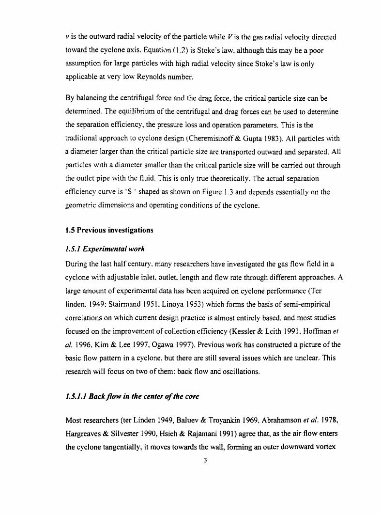
v is the outward radial veiocity of the particle while Vis the gas radiai velocity directed
toward the cyclone asis. Equation (1.2) is Stoke's iaw. although this may be a poor
assumption for large particles with high radial velocity since Stoke's law is only
applicable at very low Reynolds number.
By balancing the centrifuga1 force and the drag force, the critical panicle size cm be
determined. The equilibriurn of the centrifuga1 and drag forces c m be used to determine
the separation efficiency, the pressure loss and operation parameters. This is the
traditional approach to cyclone design (Cheremisinoff& Gupta 1983). Al1 particles with
a diameter larger than the critical particle size are transported outward and separated. Al1
particles with a diameter smaller than the critical particle size will be canied out through
the outlet pipe with the fluid. This is only true theoretically. The actual separation
rfficiency curve is 'S ' shaped as shown on Figure 1.3 and depends essentially or, the
geometric dimensions and operating conditions of the cyclone.
1.5 Previous investigations
1.5.1 Experimental work
During the last half century. many researchers have investigated the gas flow field in a
cyclone with adjustable inlet. outlet. length and fiow rate through different approaches. A
large amount of experimental data has been acquired on cyclone performance (Ter
linden. 1 949: S tairmand 195 1. Linoya 1 953) which foms the basis of semi-empirical
correlations on which current design practice is almost entirely based. and most studies
focused on the improvement of collection efficiency (Kessier & Leith 199 1 . Hoffman et
al. 1996. Kim & Lee 1997, Ogawa 1997). Previous work has constructed a picture of the
basic flow pattern in a cyclone. but there are still several issues which are unclear. This
research witl focus on two of them: back flow and oscillations.
1 S.1.1 Bock flow in the center of the core
Most researchers (ter Linden 1949, Baluev & Troyankin 1969, Abraharnson et al. 1978,
Hargreaves & Silvester 1990, Hsieh & Rajamani 1991) agree that, as the air flow enters
the cyclone tangentially, it moves towards the wall, forming an outer downward vortex
3
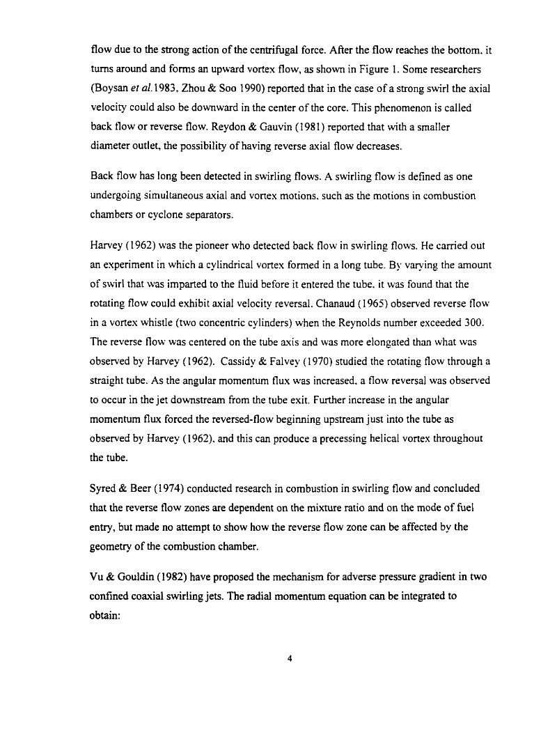
flow due to the strong action of the centrifuga1 force. Afier the flow reaches the bottorn. it
turns around and forms an upward vortex flow, as s h o w in Figure 1. Some researchers
(Boysan et al. 1983, Zhou & Soo 1990) reported that in the case of a strong swirl the axial
velocity could also be downward in the center of the core. This phenornenon is called
back tlow or reverse fiow. Reydon & Gauvin (1 98 1) reported that with a smaller
diameter outlet, the possibility of having reverse axial flow decreases.
Back flow has long been detected in swirling flows. A swirling 80w is defined as one
undergoing simultaneous axial and vonex motions. such as the motions in combustion
chambers or cyclone separators.
Harvey (1962) was the pioneer who detected back fîow in swirling flows. He cax-ried out
an experiment in which a cylindrical voriex fomed in a long tube. By v q i n g the arnount
of suirl that was imparted to the fluid before it entered the tube. it was found that the
rotating flow could exhibit axial velocity reversal. Chanaud (1 965) observed reverse flow
in a vortex whistle (two concentric cylinders) when the Reynolds number exceeded 300.
The reverse flow was centered on the tube avis and was more elongated than what was
observed by Harvey (1962). Cassidy 8: Falvey (1970) studied the rotating flow through a
straight tube. As the angular momentum flux was increased. a flow reversal was observed
to occur in the jet downstream From the tube exit. Further increase in the angular
momentun flux forced the reversed-flow begiming upstrearn just into the tube as
observed by Harvey (1962). and this can produce a precessing helical vortex throughout
the tube.
Syred & Beer (1974) conducted research in combustion in swirling flow and concluded
that the reverse flow zones are dependent on the mixture ratio and on the mode of fuel
entry, but made no attempt to show how the reverse flow zone can be affected by the
geometry of the combustion chamber.
Vu & Gouldin (1982) have proposed the mechanism for adverse pressure gradient in two
confined coaxial swirling jets. The radial momentum equation c m be integrated to
obtain:
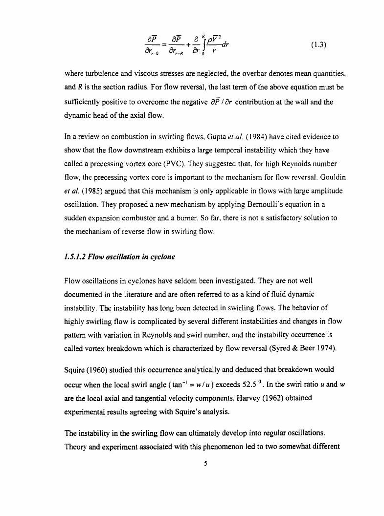
where turbulence and viscous stresses are neglected, the overbar denotes rnean quantities.
and R is the section radius. For flow reversal, the last term of the above equation must be
sufficiently positive to overcome the negative 8%- contribution at the wdl and the
dynamic head of the axial flow.
In a review on combustion in swirling flows. Gupta rr dl. (1 983) have cited rvidence io
show that the flow downstream exhibits a large temporal instability which they have
called a precessing vortex core (PVC). They suggested that. for high Reynolds number
flow, the precessing vortex core is important to the mechanism for flow reversal. Gouldin
et al. ( 1 985) argued that this mechanism is only applicable in flows with large amplitude
oscillation. They proposed a new mechanism by applying Bernoulli's equation in a
sudden expansion combustor and a bumer. So far. there is not a satisfactory solution to
the mechanism of reverse flow in swirling flow.
1.5.1.2 Flow oscillalion in cyclone
Flow oscillations in cyclones have seldom been investigated. They are not well
docurnented in the literature and are olten referred to as a kind of fluid dynamic
instability. The instability has long been detected in swirling flows. The behavior of
highly swirling flow is complicated by several different instabilities and changes in flow
pattern with variation in Reynolds and swirl number. and the instability occurrence is
called vortex breakdown which is characterized by flow reversal (Syred & Beer 1974).
Squire ( 1960) studied this occurrence analytically and deduced that breakdown would
occur when the local swirl angle ( tan-' = w / u ) exceeds 52.5 O . In the swirl ratio u and w
are the local axial and tangentid velocity components. Harvey (1962) obtained
experimental results agreeing with Squire's analysis.
The instability in the swirling flow can ultimately develop into regular oscillations.
Theory and expenment associated with this phenornenon led to two somewhat different
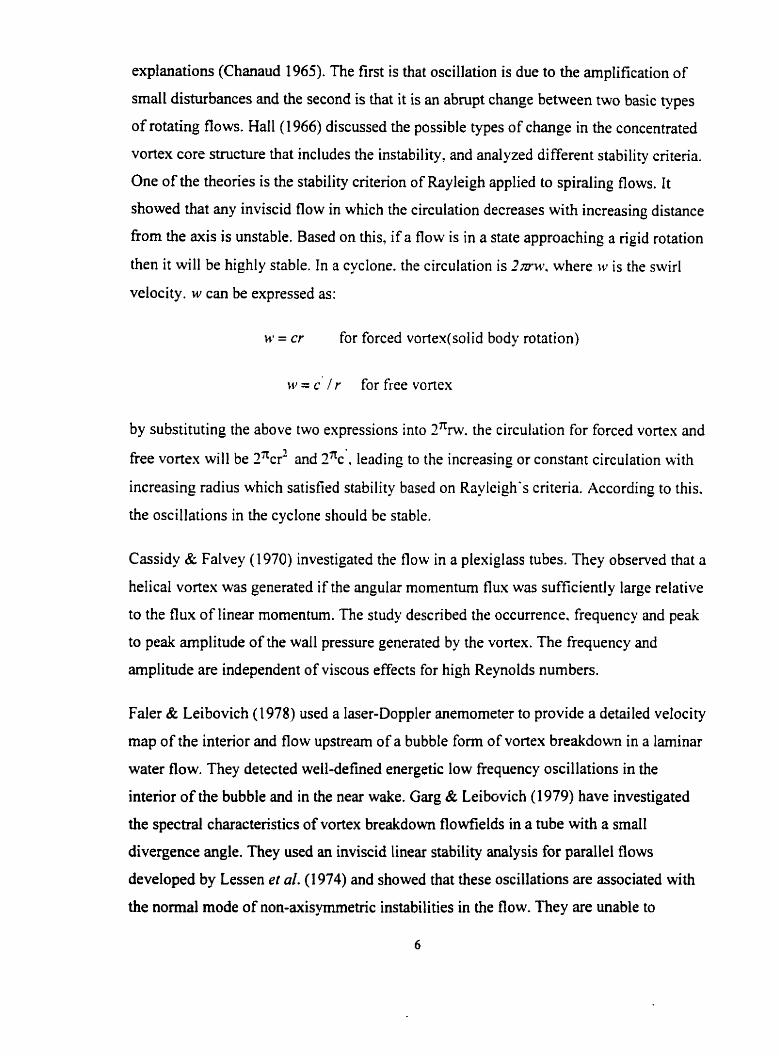
explanations (Chanaud 1965). The first is that oscillation is due to the amplification of
smdl disturbances and the second is that it is an abrupt change between two basic types
of rotating flows. Hall (1 966) discussed the possible types of change in the concentrated
vortex core structure that includes the instability, and analyzed different stability criteria.
One of the theories is the stability criterion of Rayleigh applied to spiraling flows. It
showed that any inviscid flow in which the circulation decreases with increasing distance
60m the axis is unstable. Based on this, if a flow is in a state approaching a ngid rotation
then it will be highly stable. In a cyclone. the circulation is Zmiv. where IV is the swirl
velocity. w c m be expressed as:
w = cr for forced vortex(solid body rotation)
w = c l r for free vortex
by substituting the above two expressions into Znw. the circulütion for forced vortex and
free vortex will be I%? and 2%'. leading to the increasing or constant circulation with
increasing radius which satisfied stability based on Rayleigh's criteria. According to this.
the oscillations in the cyclone should be stable.
Cassidy & Falvey (1 970) investigated the flow in a plexiglass tubes. They observed that a
helical vortes was generated if the angular momentum flux aas sufficiently large relative
to the flux of linear momentum. The study described the occurrence. frequency and peak
to peak amplitude of the wall pressure generated by the vortex. The frequency and
amplitude are independent of viscous effects for high Reynolds numbers.
Faler & Leibovich (1978) used a laser-Doppler anemometer to provide a detailed velocity
map of the interior and flow upstream of a bubble form of vortex breakdown in a laminar
water flow. They detected well-defhed energetic low ffequency oscillations in the
intenor of the bubble and in the near wake. Garg & Leib~vich (1979) have investigated
the spectral characteristics of vortex breakdown flowfields in a tube with a small
divergence angle. They used an inviscid linear stability analysis for parallel fiows
developed by Lessen et al. (1 974) and showed that these oscillations are associated with
the normal mode of non-axisymmetric instabilities in the flow. They are unable to
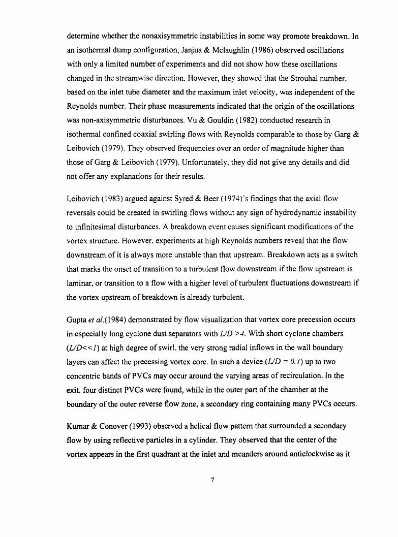
determine whether the nonaxisymmetric instabilities in some way promote breakdown. In
an isothemal dump configuration, Janjua & Mclaughlin (1 986) observed oscillations
with ody a limited number of experiments and did not show how these oscillations
changed in the streamwise direction. However, they showed that the Strouhal number.
based on the inlet tube diarneter and the maximum inlet velocity, was independent of the
Reynolds nurnber. Their phase rneasurements indicated that the origin of the oscillations
was non-axisymmetric disturbances. Vu & Gouldin (1 982) conducted research in
isothemal confined coaxial swirling flows with Reynolds comparable to those by Garg &
Leibovich (1 979). They observed fiequencies over an order of magnitude higher than
those of Garg & Leibovich (1979). Unfortunately. they did not give any details and did
not offer any explanations for their results.
Leibovich (1 983) argued against Syred & Beer ( 1974)'s findings that the axial flow
revenais could be created in swirling flows without any sign of hydrodynamic instability
to infinitesimal disturbances. A breakdown event causes significant modifications of the
vortex structure. However. experiments at high Reynolds numbers reveal that the flow
dow-nstream of it is always more unstable than that upstrearn. Breakdown acts as a switch
that marks the onset of transition to a turbulent flow downstream if the flow upstream is
laminar, or transition to a flow with a higher level of turbuient fluctuations downstream if
the vortex upstrearn of breakdown is already turbulent.
Gupta et aL(1984) dernonstrated by flow visualization that vortex core precession occurs
in especially long cyclone dust separators with U D W . With short cyclone chambers
(UD<<I) at high degree of swirl. the very strong radial inflows in the wall boundary
layers c m affect the precessing vortex core. In such a device (L/D = 0.1) up to two
concentric bands of PVCs may occur around the varying areas of recirculation. In the
exit. four distinct PVCs were found, while in the outer part of the chamber at the
boundary of the outer reverse flow zone, a secondary ring containing many PVCs occurs.
Kumar & Conover (1 993) observed a helical flow pattern that surrounded a secondary
80w by using reflective particles in a cylinder. They observed that the center of the
vortex appears in the first quadrant at the inlet and meanders around anticlockwise as it

traverses the length of the cylinder. The vortex center in the cross sections is observed to
be stable but not steady. This center would frequently move fiom its average location.
Bernard (1992) observed oscillations in his flow visualization in a cycione and concluded
that not only the turbulence of the flow pattern but also the construction of the cyclone
and the way the flow is introduced into the cyclone might cause the instability.
Experiments by Yazdabadi et al. (1994) show that as the Reynolds number is increased, a
large three dimensional time dependent instability develops just outside the vortex finder
of the cyclone. and the flow field in that region oscillates with a regular frequency and
amplitude. For ir to be a stable oscillation, there must be a feedback mechanism. and it
has been suggested that this is provided by the reverse flow zone in the vortex finder. The
oscillation is greatly affected by the swir! number defined as the ratio of the mial flux of
swirl momentum to the z ~ i a l flux of axiai mornentum.
1.5.2 N~imerical work
Early in the nineteen seventies. Kopecky 8: Torrance ( 1 973) and Grabowski & Berger
(1976) carried out numerical computations of steady. lamina. avisymmetric Navier-
Stokes equations in attempts to simulate the back flow. The results obtained by them
differ from experiments in the following ways:
a): The numerical solutions do not reveal the two-celled structure in the interior of the
recirculation zone revealed by the tirne-averaged strearnlines constructed from the
experimental data of Faler (1 976).
b): Back flow has never been seen at low Reynolds numbers such as those used in the
computations.
In the last 15 years, a theoreticai approach based on the calculation of the actual flow
field fiom the Navier-Stokes equations has become more popular thanks to the
development of faster cornputers with more memory. After the gas flow field is
calculated, the motion of single particles introduced into the flow c m be tracked. By
cdculating particle paths for different size particles, a separation eficiency curve can be
determined. Such an approach is valid for dilute slurries only. since only in this kind of
flow particle-particle interactions can be neglected. The fluid motion is not affected by
the contributing source terms in the Navier-Stokes equations due to particle-fluid
interaction. but the influence from the surrounding gas on the particle is retained. (Frank
et al. 1998)
For the turbulent flow field in a cyclone, the key to a successful computation lies in the
accurate description of turbulent behavior of the fiow. According to Hanjalic (1 994).
three types of turbulence models coufd be identitied as fast engineering methods (despite
the nerd to solve partial differential equations)
O two-ciquation rddy-viscosity models (k-r)
O the difkrential Reynolds stress rquation model (RSM) (differential second-moment
closure): and
O intermediate (truncated) and hybrid models that hierarchically fa11 in betwecn these
two and take somç advantages from each of them (ASM)
The k-smodel in its nidimentary form has a major advantage in its simplicity and
practical usability. Zhou & Soo ( 1 990) assume non-theta gradients and applied the k-E
turbulence mode1 to solve the tangential and axial velocity in a cyclone. In the near-axis
region. the numerical predictions give much higher values than those obtained frorn
measurements. The discrepancy is a result of the defect of the k-grnodel. which cannot
account for the non-isotropic turbulence structure due to the di fferent magnitudes of
velocity components and hence gives high values of the turbulent viscosity, leading to a
high axial velocity near the auis.
Many researchers made modifications to the k-~model, Yap's (1 987) proposa1 stands out
as one interesting theory because he thinks the k-E produces near-wall length scales that
are too large; he therefore added a source terni in the ,s equation. Minier et aL(199 1)
consider Yap's (1 987) model as an attractive and inexpensive alternative to the complete
RSM model if k-E shortcomings are to be overcome.

The Reynolds-stress model (RSM) is regarded as the natural and most logical level of
modeling within the framework of the Reynolds averaging approach. Since it provides
the extra turbulent momenhim fluxes from the solution of full transport equations, it
requires a length-scale-supplying equation. Although the Reynolds stress model performs
much better than the k-&mode1 in swirling flow because it accounts automatically for the
effects of stress anisotroy, it has the disadvantage of being computationally expensive.
An intemediate solution might be to use the algebraic stress model (ASM) which
transforms the differential equations into algebraic ones and leads to direct expressions
for the Reynolds stress components. The development of the ASM raised two
coefficients, incorporating a total of nine new parameters. Boysan et al. (1 987) developed
this model and found better than expected agreement with certain regimes of swiriing
flow. Hoffman er al. (1 996) predicted back flow using a 2-dimensional ASM modei. The
length of the vortex finder has a very imponant effect on the appearance of back flow.
However. some authors argue that the algebraic stress model should not be used for
;~uisymmetnc swirling flow. Fu et al. (1 986) emphasized that despite the significant tirne
savings. the ASM scheme ought not to be used where stress-transport processes give rise
to significant t ems in the overall Reynolds stress.
So far. the differential Reynolds stress model (RSM) is the most promising turbulence
model for descnbing the swirling cyclone flow. Boysan ( 1984) predicted reverse flow in
the cyclone using RSM. Mees'(I997) 3D simulations using CFX software (from AEA
technology) with the RSM model also show oscillations in the body of the cyclone.
Researchers are still not sure about the proper boundary conditions at the two cyclone
outlets because of insufficient experimental data. Usually, fully developed flow boundary
conditions are imposed at the exits.
1.6 Approach used in this work
The objective of this work is to investigate the existence of the three dimensional time
dependent instability in the body of the cyclone, and examine back flow in the cyclone
under the influence of various gas outlet geornetries. Experiments were conducted in a
glas cyclone using Laser Doppler anemometry. The flow was modeled using second
order Reynolds stress closure. The results will give information valuable for the designer
about the effects of oscillation and back fiow on the separation efficiency.
Laser Doppler anemometry (LDA) was used to measure the axial and tangential
components in or just outside the gas outiet to provide boundary conditions for the
simulations. Some measurements have also been carried out in the barre1 and cone of the
cyclone.
Frequency analysis was used to analyze the low fiequency instability of the coherent
structure. The LDA time senes were analyzed using the autocorrelation fùnction and
spectral analyses. Since traditional FFT analysis cannot be ernployed for the unevenly
spaced data collected by our instrument, a slotting technique was applied.
Finally, 3D tmsient CFD simulations were carried out to validate the mode1 with the
ultimate aim of predicting flow in other geomeiries. The Reynolds stress mode1 of
turbulence was used. The effects of inlet velocity and boundary conditions were
examined.
Figure 1.1 Cyclone geometry and general flow pattern
Figure 1.2 Cross-sectional dimensions of a reverse flow cyclone
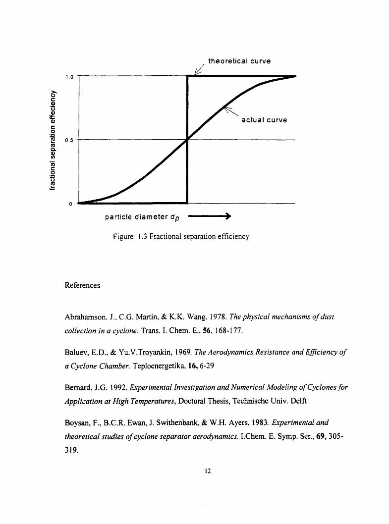
/ theoretical curve
particle diameter d p -> Figure 1.3 Fractional separation efficiency
Re ferences
Abraharnson. J.. C.G. Martin, & K.K. Wang. 1978. The physical mechanisms of dust
colleczion in a cyclone. Trans. 1. C hem. E.. 56. 1 68- 1 77.
Baluev, E. D., & Yu.V.Troyankin, 1969. The Aerodynarnics Resistance und Eflciency of
a Cyclone Chamber. Teploenergeti ka. 16,6-29
Bernard. J.G. 1992. Erperimental Investigation and Numerical Modeling of Cyclones for
Application ut High Temperatures, Doctoral Thesis, Technische Univ. Del fi
Boysan, F., B.C.R. Ewan, J. Swithenbank, & W.H. Ayers, 1983. Experimental and
haretical studies of cyclone separator aerodynamics. L .Chem. E. S ymp. Ser., 69,3 05-
319.
Boysan. F., 1984, Mathemafical modeling of cyclone sepuration, Proceedings o f 9"
lecture series on two-phase flow, Trondheim, Nonvay.
Chanaud. Robert C., 1965, Observations ofoscillatory motion in certain swirlingfToivs. J.
Fluid Mech. 2 1. 1 1 1 - 127
Cherernisinoff. NP.. & R. Gupta. 1983. Handbook of Fhids in Motion. 847-860
Cassidy, John J.. & Henry T . Falvey, 1 970. Observations of unsteady floiv arising after
vorrex breakdorvn. J.Fluid Mech. 41,737-736
Faler, J.H.. & S . Leibovich, 1 978. An e.rperimenta2 oj'vorrex brrukdu>t~njloi~$c'Id.~..
Journa1 o f fluid rnechanics, 86. 1978
Frank. E.. and Yu. Q. Wassen. 1 998, Lrrgrangian prediction oj'disperse gas-particle Joie in cyclone separutors. Third international conference on multiphase tlow. Lyon. France
June 8- 12.1998. CD-ROM. Paper No. 2 17
Fu. S.. P.G. Huang. B. E. Launder. & MALeschziner. 1988. il Comparison of.-Ugebruic
and Diffirential Second-Moment Closurrs For ttrrbuleni Shrar F low with and withoirt
Swirl. Transactions o f the ASME 1 f O, June. 2 16-22 1
Garg, A. K.. & S . Leibovich. 1979. Spectral characteristics of vortex breakdo wn
flowfields, Physics o f fluids. 22, 1979.2053-2064
Gouldin, F.C., J.S. Depsky, & S-L. Lee. 198% Velociryfield characreristics of a swirling
jlow cornblrstor. AIAA Journal 23,950 102
Gupta, A. K.. D.G. Lilley, & N.Syred. 1984. Swirlflow. Energy and Engineering Science
Series
Hall, M.G., 1966. The structure of concentrated vortex cures. Progress in Aeronautical
Sciences. 7,53- 1 10
Hanjalic,K., 1 994, Advanced rurbulence closure mode!: A view of current status and
M u r e prospect. Int. J Heat and fluid Flow. 15 June 178-203
13
Hargreaves, J.H., & R.S. Silvester. 1 990. Computationalfluid dynamics opplied to the
analysis of hydrocyclone performance. Trans IChemE..68. Part A. 365-383
Harvey, J.K. 1 962. Some observations of the vortex breakdo~t~n phenornenon. J. lu id Mech. 14,585
Hoffmann. AC.. de Groot. & M. Hospers, A. 1996. The Effect of the Diisf Collection
Systern on the Flow pattern and Separation Efficiency of a Gus Cyclone. The Canadian
Journal of Chernical Eng.. 74.464470
Hsieh. K.T.. & R.K. Rajamani. 199 1. Maihematical Mode/ of the Hydrocyclone Bused on
Physics of Flirid Flow. AIChE Journal. 37(5). 735-746
Janjua. S. 1.. and D. K. MaLaughlin. 1 986. il n rxperimmtol siudv on sivirling confinrd
jets wiih heliunl injection. Rept. DT-8561-01. Dynamics Technology. Inc. Torrance. CA
Kessler. Marc & D. Leith. 199 1. Flow measzrrrrnent and eficiency rnodelinp ofcyclones
for particle collection. Aerosol Science and Technology. 15, 8- 1 8
Kim. W.S.. & J. W.Lee. 1997, Collection efficiency model based on boundary-layer
characteristicsfor cyclones. AIChE Journal. 43.2446-2455
Kopicky, R. M. & K. E. Torrance, 1 97 1 , Initiarion and struaure of~xisymmetric eddies in
a rotating stream, Cornpurers and Fhids. Computers and Fluids. 1.289
Kumar. R., T. Conover, 1993. FIow visulkurion sritdies of a swirlingfloiv in a cyiinder.
Experirnental Thermal and Fluid Science. 7.254-262
Leibovich, S.. 1984, Vortex stability and breakdown: siinvy and extension. AIAA
Journal, 22, 1 192- 1206.
Lessen, M., P. J. Singh, & F. Paillet, 1974, The stability of a trailing line vortex Part 1.
Inviscid Theory, humai o f Fluid Mechanics. 63,753 -763.
Linoya, K., 1953, Study of lhe cyclone, Memoirs of the Engineering, Nagoya University,
5, 131-178
Loffler, F., M. Schmidt, & R. Kirch. 199 1. EsperimentaZ investigation into gus cyclone
jlowfiekds zrsing a laser-doppler-i~elocimeter. Indusrie Minerale-Mines et carrieres. les
Techniques. July. 149- 1 56
Mees, P.A.J., 1997. Three dimensional transient gus cyclone simulations. 47" Canadian
Chemical Engineering Conference. Oct. 5-8. Edmonton, Alberta. Paper 482.
Minier. J.P.. Simomon. O.. & Babillard, M. 199 1. Nttmerical rnodelling of cyclone
separafors. Fllririixci hrt? con~hosrion. AS ME 125 1 - 1159.
Ogawa, 4.. 1 997. mech ha ni cal separation proress andjlow patterns of c-vcfone drist
collecfors. Xppl Mech Rev 50.97-1 30
Reydon. R.F.. & W. H.Gauvin. 198 1 . Throrrtical und Exprrimentul Stutlies of'Confinrd
Vorrex Flow. The Canadian Journal of Chemical Eng.. 59. 14-23
Squire. H. B. 1960, .4ncifpis of iltr ïorrex hrcokdown phenornena. Part 1 . Aero. Dept..
Imp. C d . Rep. No. 1 O?
S tairmand. C . J.. 1 95 1 . The design nndpei@muncr oj'cyclone sepurators. Trans. Inst.
Chem. E.. 29 356-383.
Syred. N.. & J.M. Beer. 1974. Comhmtion in sivirlingflows: a review. Combustion and
flarne. 23. 143-20 1
ter Linden. A.J., 1949. Invesligation inro cyclone dmt collecrors. Proc. 1. Mech. E.. 160,
Vu. B.T.. & F.C. Gouldin, 1982, FZoiv measiirements in u mode1 swirl combustor, AIAA
Journal. 20,643-65 1
Y ap, C . L. 1 987. Turbulent Heat and iWornenturn Transfeer in Recirculating and Impinging
Flows. Ph.D. Thesis. UMIST, Manchester
Yazdabadi, P.A., A.J. Grifiths, & N . Syred. 1994, Investigations into the precessing
vortex core phenornenon in cyclone dust sepmators. Proc. 1. Mech. E., 208, 147-1 54.

Zhou, L.X., & S.L. Soo, 1990, Gas-Solidflow and collection of solid in a Cyclone
separutor. Powder Tech., 63,4543.

Chapter 2: Experimental
In this chapter, the theory of laser Doppler anemometry, the LDA system used in this
work. the experimental design, and the seeding methods for this high velocity field are
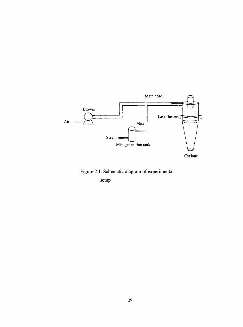
discussed. A schematic diagram of the expenmental equipment is shown in Figure 2.1.
The main components are the LDA, the tank where the seeding particles are generated,
the g l a s cyclone, and the blower that provides the airflow. Each of these components is
discussed in tum.
2.1 The principle of laser Doppler anemometry (LDA) - an overview
With the invention of the laser in 1960 it was natural that people should stai-t considering
rneasuring the velocity of a matenal by means of the 'Doppler effect'. This technique
allows the measurement of the local. instantaneous velocity of tracer particles suspended
in the flow without disturbing the flow with a probe. It provides great advantages in
recircuiating flows. such as cyclones and in flows in ducts of srnaIl dimensions where
mechanical probes can cause interference or blockage.
The basic principles of laser Doppler anemometry c m be interpreted as fotlows: when a
beam of light with a certain frequency reaches a moving object. the frequency of the light
will be changed. To construct the LDA measuring volume. two laser bearns are directed
to the location at which the measurement of the velocity is required. The relation between
the Doppler shift frequency f, and the velocity of a moving object scattering the light is
(Drain, 1980)
where V is the velocity of the object, 0 is the angle between two illurninating bearns, and
i$, is the wavelength of the light. %y measuring the Doppler shift fiequency for a given
wavelength and beam angle, the velocity of the moving object can be determined.
In our lab, the LDA uses a 300mW argon-ion laser manufactured by Ion Laser
Technology, operating at a 5 14.7 nm wavelength green beam. The system is one

component and uses fonvard scattering: scattered light is collected opposite the source of
the light.
In our system, the dual beam or differential Doppler technique is used in which the
rneasurement volume is illuminated by two focused, coherent laser beams of sirnilar 0 intensity and at beam angle intersection. as shown in Figure 2.2. n i e beams overlap to
form an ellipsoidal measuring volume. The pattern of altematively dark and bright planes
with a known spacing is known as fnnges. As each particle crosses the fringes, the
intensity of light scattered ont0 the detector rises and fails at a frequency ( j») directly
proportional to the velocity.
The fringe spacing, 6, . is dependent on the wavelength of the light &, and the beam
intersection angle. 8. and is given by
In our case. the argon-ion laser provides the monochromatic and coherent light source.
There are three different tracks, which provide three beam spacing and intersection
angles. The two beams of equal intensity emerge from the transmitting optics through an
f = 500 mm focal length lens and intersect at angles 0 = 1.94. 3.88. and 7.1 9 degrees.
depending on which track is chosen. resulting in spacings of the interference fnnges in
the measuring volume of 6/ = 15.2.7.6. and 4.1 h respectively. The number of fnnges
in the probe is N = 18 . Most expenments were conducted on track 1, since it has a higher
data rate.
In measuring recirculating or turbulent flows, the direction of velocity is unknown before
hand. To avoid velocity direction ambiguity, a Bragg ce11 frequency shift is employed.
The fùnction of the Bragg ce11 is to introduce a fixed optical fiequency shift f, on one
beam. The shifted beam has the same opticd properties as the incoming beam and causes
no deterioration of the performance of the laser Doppler system. Frequency shifting may

be described as a modulation of shifiing frequency, y = A. - 6, , where f , is the
modulation frequency shift introduced, and 6f is the fringe spacing. Thus a flow moving
against the fnnge pattern will result in an increase in the frequency of the light scattered
fiom a particle in the measuting volume by an arnount f, , where f, is the Doppler shift
due to the particle motion. In other words. the detected frequency is f, = + f , . taking
into account the sign of f, . For Aerometrics' Bragg ce11 trammitter system, a 40MH=
fiequency shifi is set. Since the optical frequency shift is not infinitely adjustable, an
electronic frequency shift. i.e. mixer frequency is employed afier the photodetector. The
electronic shifting increases the center Frequencies of both Doppler spectrum and the
pedestal. In our experiment. 35iWFiz was set for the mixer fkequency. and a lOiMH= low
pass filter was applied to attain the velocity range from -30.4- +30.4 on track 1 .
2.2 Optical system
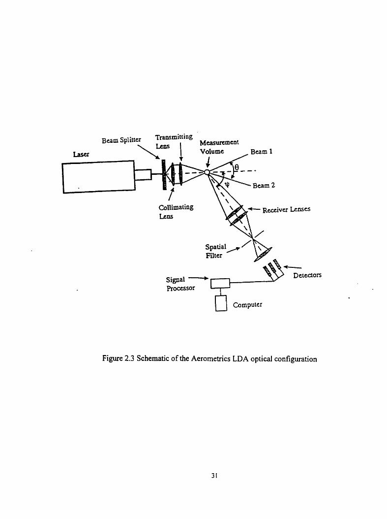
2.2.1 Optical configurations
The laser Doppler velocity measurement system consists of a laser. bearn splitter. Bragg
cell. focusing lenses. photodetectors. amplifiers and a signal processor. as shown in
Figure 2.3. The two beams are denved from a continuous - wave laser beam using a
beam splitting prism. They are then passed through a collimating lens. The Bragg ce11
applies a frequency shift to one beam. They are focussed by the transmitting lens ont0 the
measuring volume. The measuring volume is intersected by the focal plane of the
imaging system formed by the receiver and the photodetector aperture. Light scattered by
a traversing particle is imaged on the photodetector. The resulting electrical signal is fed
to a signal processor to extract the Doppler frequency. In our system, a Doppler signal
analyzer (DSA) uses frequency domain burst detection to convert signals. The advantage
of this method is that it can be successfùlly applied to a low signal to noise ratio signal.
2.2.2 Optical requiremenb und comportent measured N, the study
In LDA, there are some optical limitations to successfbl measurement. A velocity
measurement cannot be acquired in al1 places where the measuring volume can be
located.
In LDA, two beams pass through the fluid and intersect to form the measuring volume. In
the case of measurements in confined or intemal flows, the incident beams pass from the
air through a transparent wall or window before entering the fluid under consideration.
The laser beams are refracted at the solid interfaces between these media. Sornetimes, the
refiaction will produce a difference in optical path length between the two beams, andor
a change in the orientation of the beam angle bisector (thus measunng a different
component of velocity than intended), as well as a change in the position of the
measuring volume. (Kresta 1991 )
For an experimental system with fixed refractive indices and tube radii. the refraction
effects for measurement can always be calculated by applying Snell's law of refraction
and ray tracing (Gardavsky et al. 1989). This is required to determine if the velocity
component c m be measured by LDA. In our system. before canying out experlments.
calculations were done to determine the accessible measuring locations and the velocity
components actually measurrd.
Refraction effects in the cyclone are cornplex due to the curved and tilted geometry. since
the cyclone geometry is composed of a cylinder and a cone. In the calculation. the
cylinder is a planar geometry in the measurement of axial velocity. and a circular
geometry for the radial and tangential components of velocity. There can be no difference
in optical path length or deviation angle in measurement of the axial and tangential
velocities in the cylinder because the two beams are always symmetric to the centerline
(Figure 2.4A). Unlike the measurement of tangential velocity, the measurement of the
radial component requires the two beams to be moved sideways with respect to the
centerline, as shown in Figure 2.4B. In this case, the real bisector between the bearns at
the point of intersection is not always tangent to the circle but c m be at a small angle 4. the deviation angle, as shown in Figure 2.5. The two beams may now have a difference in
path length. A deviation angle results in the measurement of a srnall component of
tangential velocity, dong with the radial velocity. Although this angle is insignificant in
the cylinder, the radial velocity measurement is unreiiable since the tangential velocity is
100 times larger than the radial velocity.
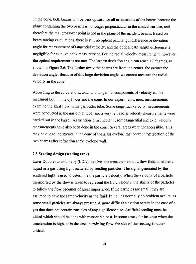
In the cane' both bearns will be bent upward for a11 orientations of the beams because the
plane containing die two bearns is no longer perpendicular to the conical surface, and
therefore the real crossover point is not in the plane of the incident beams. Based on
beam tracing calculations, there is still no optical path length difference or deviation
angle for measurement of tangential velocity, and the optical path length difference is
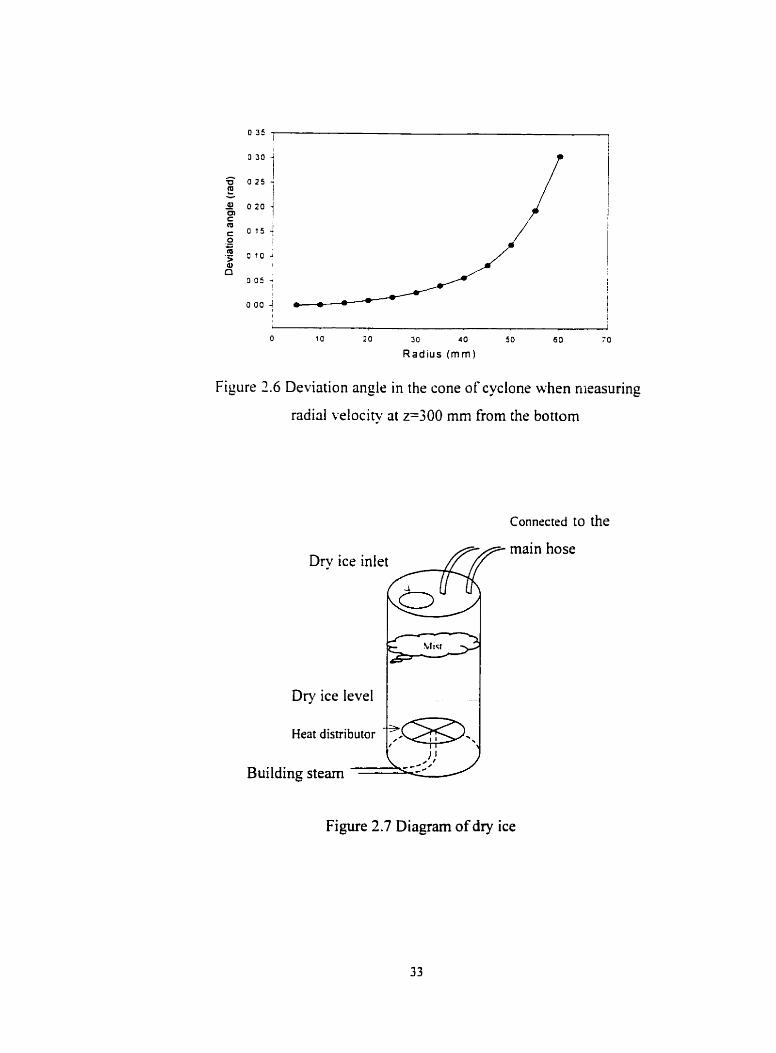
negligible for avial velocity measurement. For the radial velocity measurement. however.
the optical requirement is not met. The largest deviation angle c m reach 17 degrees. as
shown in Figure 1.6. The hrther away the beams are frorn the center. the ereater the
deviation angle. Because of this large deviation angir, we cannot measure the radial
velocity in the cone.
According to the calculations. axial and tangential components of velocity c m be
measured both in the cylindrr and the cone. In Our experiments. most measurements
examine the mial flow in the gas outlet tube. Some tangential velocity rneasurements
were conducted in the pas outlet tube. and a very few radial velocity measiirements were
carrird out in the barrel. As mentioncd in chapter 1. some tangential and axial velocity
measurernents have also been done in the cone. Several areas were not accessible. This
may be due to the streaks in the cone of the glass cyclone that prevent intersection of the
two bearns afier refraction at the cyclone wall.
2.3 Seeding design (seeding tank)
Laser Doppler anemometry (LDA) involves the measurement of a flow field. in either a
liquid or a gas using light scattered by seeding particles. The signal generated by the
scattered light is used to determine the particle velocity. When the velocity of a particle
transported by the flow is taken to represent the fluid velocity, the ability of the particles
to follow the flow becomes of great importance. If the particles are small, they are
assumed to have the same velocity as the fluid. In liquids normally no problem occurs, as
some srnall particles are always present. A more dificult situation occurs in the case of a
gas that does not contain particles of any significant size. Artificial seeding must be
added which should be done with reasonable cost. In some cases, for instance when the
acceleration is high. as is the case in swirling flow. the size of the seeding is rather
critical.
Particles whose motion is used to represent that of a fluid continuum should be
able to follow the 80w;
O good light scatterers;
a conveniently generated;
cheap;
a non-toxic. non-corrosive. non-abrasive;
O non-volatile. or slow to evaporate;
a chemically inactive;
a clean.
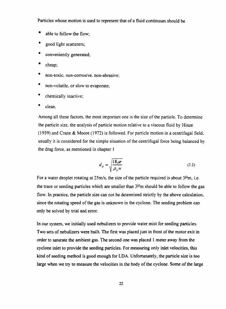
Among all these factors. the most important one is the size of the particle. To determine
the particle size. the analysis of particle motion relative to a viscous fluid by Hinze
(1 959) and Crane & Moore (1 972) is followed. For particle motion in a centrifuga1 field.
usually it is considered for the simple situation of the centrifuga1 force being balanced by
the drag force. as mentioned in chapter 1
For a water droplet rotating at 25m/s. the size of the particle required is about 3 h , i.e.
the trace or seeding particles which are smaller than 3pm should be able to follow the gas
flow. In practice, the particle size can not be determined strictly by the above calculation.
since the rotating speed of the gas is unknown in the cyclone. The seeding problem can
only be solved by trial and error.
In Our system, we initially used nebulizers to provide water mist for seeding particles.
Two sets of nebulizers were built. The first was placed just in fiont of the motor exit in
order to saturate the arnbient gas. The second one was placed 1 meter away fiom the
cyclone inlet to provide the seeding particles. For measuring only inlet velocities, this
kind of seeding method is good enough for LDA. Unfortunately, the particle size is too
large when we try to measure the velocities in the body of the cyclone. Some of the large

water droplets impinge on the wail of the transporting hose due to the inertia of the
denser water dropiets. Some of the particles are larger than the cntical separation size, so
they stay in the outer downward flow in the cyclone and get separated. Smaller particles
have to be added into the system to measure the velocity near the center of the cyclone.
Injecting the smoke of burning Chinese incense provides a good signal. This was
achieved by lighting a bundle of incense at the inlet of the motor. After two minutes,
however, the smoke covers the cyclone wall with soot so that measurements c m no
longer be taken.
Tests showed that solid carbon dioxide or liquid nitrogen combined with hot water
generates very fine droplets. The mechanism that drives the drop generation is proposed
as follows: as the solid carbon dioxide vaporizes. it has to absorb large arnount of heat
from the environment. As this happens. the moisture in the air condenses. The white fog
generated is cornposed of water mist rather than carbon dioxide. The particle size of mist
is in the size range of 1 - 1 Opm by PDPA measurernent. In the experiment. the gas flow
rate is very high. The conesponding seeding generation rate has to be very high as well.
The hipher the rate of heating the solid carbon dioxide. the higher the seeding generation
rate. Calculaiions showed that the required heating duty for seeding is about 40 kW. This
amount of heat c m only be supplied using stearn.
The seeding used was mist in the size range of 1-10 hn generated by solid carbon
dioxide mixed with stearn. A 60cm tall. 30cm diameter stainless steel tank was built to
contain the solid carbon dioxide. Stearn entered at the bottom. A perforated pipe
distributor was used in the tank to provide uniform disuibution of steam. as shown in
Figure 2.7. To some extent, adjusting the stearn valve can control the seeding flow rate.
During the experiment, dry ice c m only fil1 one-third of the tank, since too much dry ice
will freeze the water in the distributor and block the steam. The extra room in the dry ice
tank is designed to serve as a plenum chamber to eliminate the velocity or pressure
fluctuation fiom the upstream flow, so the inlet velocity in the cyclone is only dependent
on the pressure in the tank. Two narrow passages were mounted at the top of the tank to
feed the seeding particles into the main hose. Each day, 501b dry ice were delivered from
Praxair Company to nin the seeding equiprnent.
To make optimal use of the mist, i.e. without any waste of mist in the hose before it
reaches the cyclone, thz mist was fed to the air 1 m in front of the cyclone inlet. This
consideration can be explained as follows: the relaxation time for a 1 h mist droplet is
about 300 x 10" S . Since 99% of the free velocity is obtained in five times the relaxation
time, only 0.05m is required for the particle to reach the gas speed. For the flow in the
pipe to becorne fully developed, the length needed is about 1 O times the pipe diameter
(Kundu 1990). Since the diameter of the transporting hose is 3 inches. only 0.75m is
required to reach fully developed flow. Therefore. one-meter of pipe is enough for the
seeding particles to reach the flow velocity and is also enough for the mean velocity to
reach fully developed flow before the inlet to the cyclone.
The final flow process c m be described as follows: Ambient air is suppiied from the
blower to the 3-inch hose. Having a volume of 0.043 m3, the tank provides a uniform
cascade exit pressure that maintains a constant flow rate of seeding particles. After the
gas travels almg the hose for 5 meters. it meets the seeding particles and i s well mixed
with mist which is supplied from the seeding tank. After 1 m distance during which the
flow becomes fùlly developed. the seeded gas enten the cyclone tangentially and imparts
the swirling motion in the cyclone.
2.4 Cyclone model and blower
2.4.1 Cyclone model
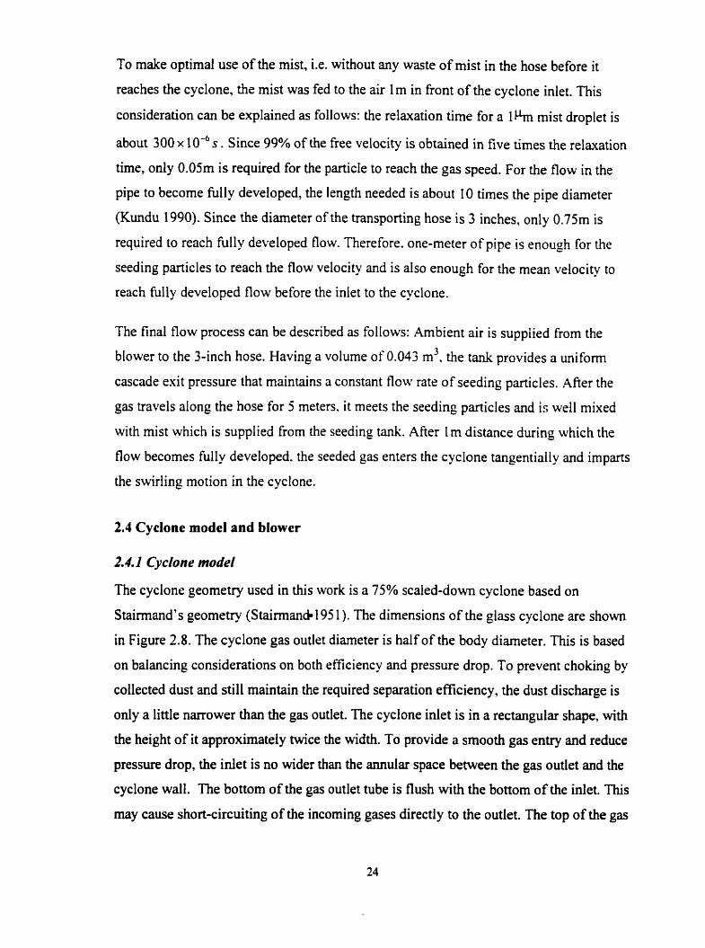
The cyclone geometry used in this work is a 75% scaled-dom cyclone based on
Stairmand's geometry (StairmancC195 1 ). The dimensions of the glass cyclone are s h o w
in Figure 2.8. The cyclone gas outlet diameter is half of the body diameter. This is based
on balancing considerations on both eficiency and pressure drop. To prevent choking by
collected dust and still maintain the required separation efficiency, the dust discharge is
only a little narrower than the gas outlet. The cyclone inlet is in a rectangular shape, with
the height of it approximately twice the width. To provide a smooth gas entry and reduce
pressure drop, the inlet is no wider than the annular space between the gas outlet and the
cyclone wall. The bottom of the gas outlet tube is Bush with the bottom of the inlet. This
may cause short-circuiting of the incoming gases directly to the outlet. The top of the gas
outlet tube is 265 mm above the roof of the cyclone. These cyclone parameters are
specified with the design of a Stairmand type cyclone. In our expenment, three gas outlet
tube diameters were used: 50 mm, 75 mm. and 95 mm, giving outlet diameter to barre1
diameter ratios of 0.3 L0.50 and 0.63.
Since the cyclone inlet is rectangular in shape. a metal piece was used to connect the
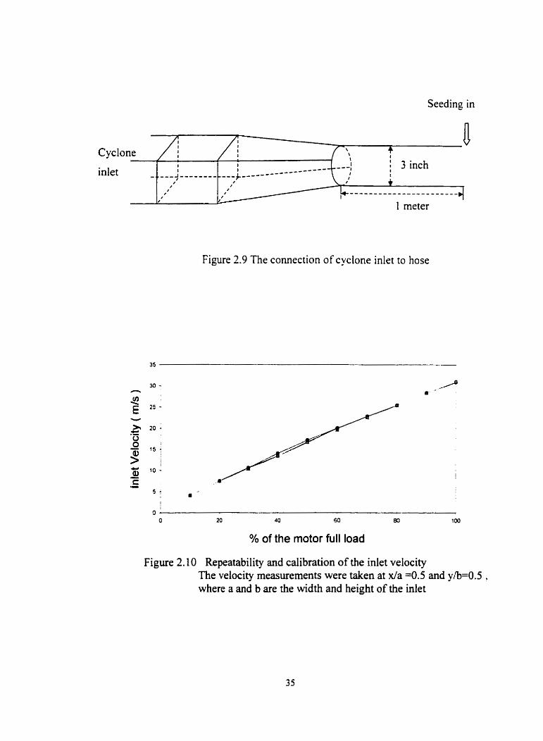
cyclone inlet to the circular cross section hose, as s h o w in Figure 2.9.
2.4.2 Blo wer
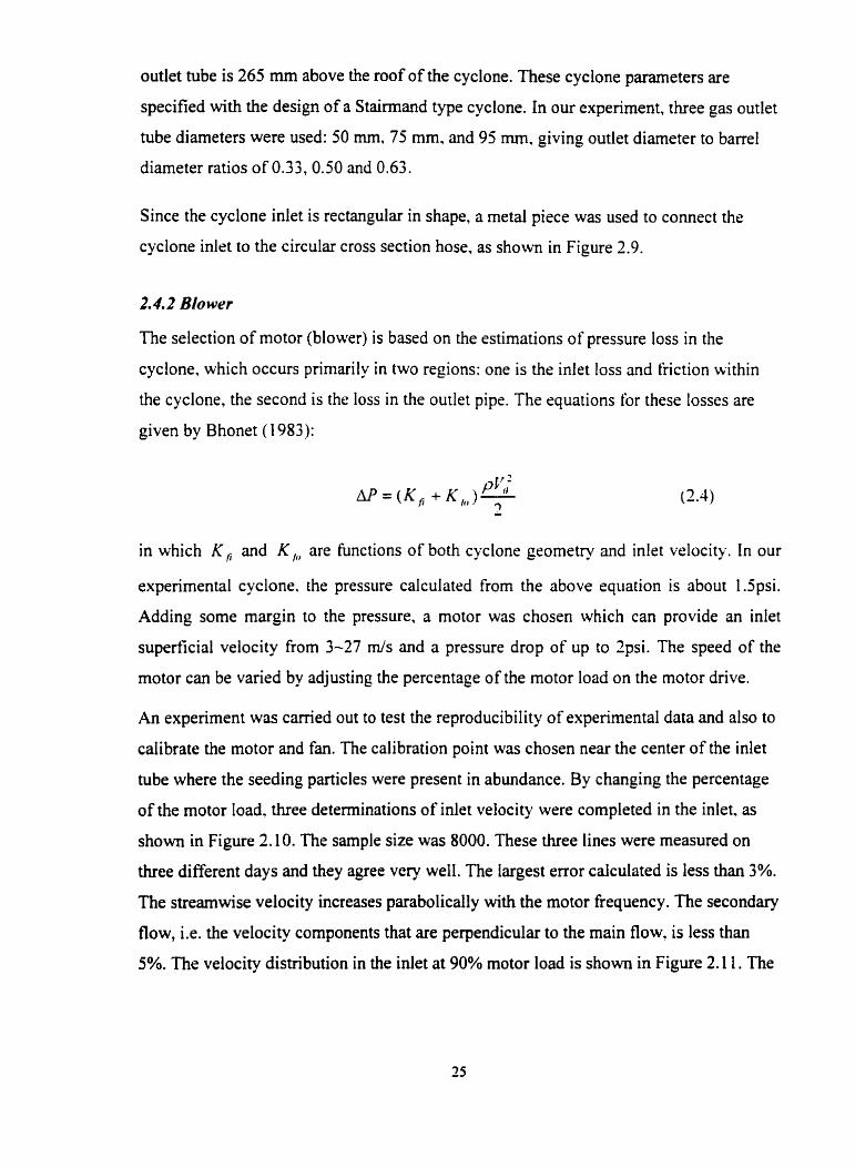
The selection of motor (blower) is based on the estimations of pressure loss in the
cyclone, which occurs primarily in two regions: one is the inlet loss and friction within
the cyclone, the second is the loss in the ourlet pipe. The equations for these losses are
given by Bhonet ( 1983):
in which K , and K,, are functions of both cyclone geometry and inlet velocity. In our
experirnental cyclone. the pressure calculated frorn the above equation is about 1.5psi.
Adding some margin to the pressure, a motor was chosen which can provide an inlet
superficial velocity from 3-27 mls and a pressure drop of up to Ipsi. The speed of the
motor c m be varied by adjusting the percentage of the motor load on the motor drive.
An experiment was camed out to test the reproducibility of experimental data and also to
calibrate the motor and fan. The calibration point was chosen near the center of the inlet
tube where the seeding particles were present in abundance. By changing the percentage
of the motor load. three determinations of inlet velocity were completed in the inlet. as
shown in Figure 2.10. The sarnple size was 8000. These three lines were measured on
three different days and they agree very well. The largest error calculated is less than 3%.
The streamwise velocity increases parabolically with the motor fiequency. The secondary
flow, i.e. the velocity components that are perpendicular to the main flow, is less than
5%. The velocity distribution in the inlet at 90% motor load is shown in Figure 2.1 1. The
distribution is quite flat in the rniddle which shows that the flow is subject to considerable
turbulence: velocity gradients only exist near the boundary.
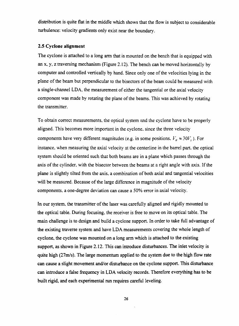
2.5 Cyclone alignrnent
The cyclone is attached to a long arm that is mounted on the bench that is equipped with
an x, y, z traversing mechanism (Figure 2.12). The bench can be moved horizontally by
computer and controlled verticaily by hand. Since only one of the velocities lying in the
plane of the bearn but perpendicular to the bisectors of the beam could be measured with
a single-channel LDA. the measuremeni of either the tangential or the axial velocity
component was made by rotating the plane of the beams. This was achieved by rotating
the transmitter.
To obtain correct rneasurements, the optical system and the cyclone have to be properly
aligned. This becomes more important in the cyclone. since the three velocity
components have very different magnitudes (e.g. in sorne positions. C i t 30K ). For
instance. when measuring the axial velocity at the centerline in the barre1 part. the optical
system should be oriented such that both beams are in a plane which passes through the
axis of the cylinder. with the bisector between the beams at a ripht angle with axis. If the
plane is slightly tilted from the axis, a combination of both axial and tangential velocities
will be measured. Because of the large difference in magnitude of the velocity
components. a one-degree deviaiion can cause a 50% error in axial velocity.
In Our system, the transmitter of the laser was carehlly aligned and rigidly mounted to
the optical table. Dunng focusing. the receiver is free to move on its optical table. The
main challenge is to design and build a cyclone support. In order to take full advantage of
the existing traverse system and have LDA measurements covering the whole length of
cyclone, the cyclone was rnounted on a long am which is attached to the existing
support, as shown in Figure 2.12. This can introduce disturbances. The inlet velocity is
quite high (27ds). The large momenturn applied to the system due to the high flow rate
can cause a slight movement andh disturbance on the cyclone support. This disturbance
can introduce a false fiequency in LDA velocity records. Therefore everything has to be
built rigid, and each experimental nin requires careful leveling.
2.6 Experiment error prediction and equipment calibration
Accurate determination of LDA data is particularly dificult. Two aspects are to be
considered. The first is the repeatability of data and the second is the absolute value of
the velocity. The first is influenced mainly by the fluctuating nature of the signal and
reproducibility of expenmental conditions. The mean velocity measurement in the
cyclone were repeatable to within 3%. The fluctuation data (rms velocity) could be
greatly affected by different LDA settings. For instance. the low pass filter, whose
function is to limit the high frequency noise band and remove the upper side band of the
mixed signal. can alter the rrns velocity if it is set too low. The value of the rms velocity
from track one rneasurement was lower than that from track two and track three due to
the large fringe spacing for track one. In order to have a consistent influence from the
settings. the LDA parameter settings were kept the sarne. In spite of this. repeatability of
the rms velocity was within 10% which is remarkably high. The vibration of the cyclone
due to the high velocity may contribute to the high error of rms velocity. Absolute value
determination is to be affected predominantly by the ratio of the measurement time scale
relative to the real tlow time scale. This is complicated by the presence of multiple time
scales. Fortunately. by sçtting the measuring time long enough and getting enough
sarnples. the velocity cm cover more than 100 cycles of the louest frequency component
we are interested in tu avoid velocity bias.
In the experiment. the mean data rate is of the order of 15OHz to JOOOHz. depending on
the location of the probe in the cyclone. As the probe approaches the outside walls. there
are more particles, and the data rate rises. In each measurement, 8000 instantaneous
velocities were recorded with a validation rate of approximately 65-85%. The signal
sarnpling rate is set at 40MH- . The signal sarnpling rate does not affect the measurement
as long as it is at least twice as much as the Doppler frequency ( f, = 1.8MHz). Zhou
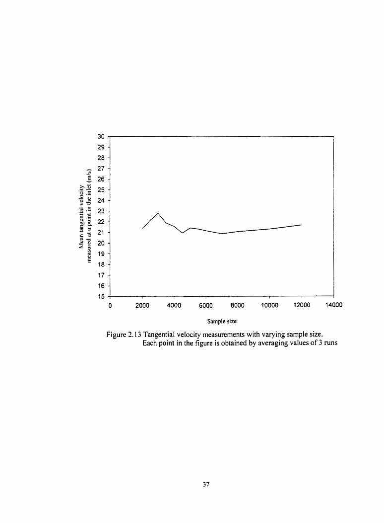
(1996) carried out the initial experiment validation. He reported that a sample size of at
l e s t 4000 is required to obtain accurate and stable rneasurement of velocities in a stirred
tank. Since the LDA settings for a cyclone are totally diflerent fiom those for a stirred
tank, repeatability tests in terms of sample size were conducted. Figure 2.13 shows that a

sample size of approximately 5000 is required to obtain repeatable results in the cyclone.
The final LDA settings are s h o w in Table 2.1 :
2.7 Conclusion
A g las cyclone was built in the lab with the gas flow provided by a blower. Since LDA
is used for the velocity field measurements. much effort has been spent on solving the
seeding problem during the setup. Mist generated by solid carbon dioxide combined with
s t e m was the solution for most experiments. Instrument calibration was camed out and
experimental repeatability was also tested with great care.
Table 2.1 Velocity setup:
High voltage (V)
Frequency shifl (MHz)
Sarnpling rate (MHz)
Sarnple size
Validation
Velocity range (rn/s)
Main hose
Cyclone
Blower
Figure 2.1. Schematic diagram of experirnental
setup
', , *'
Air Mist
Steam
Mist generation tank
Laser beams ',-Z
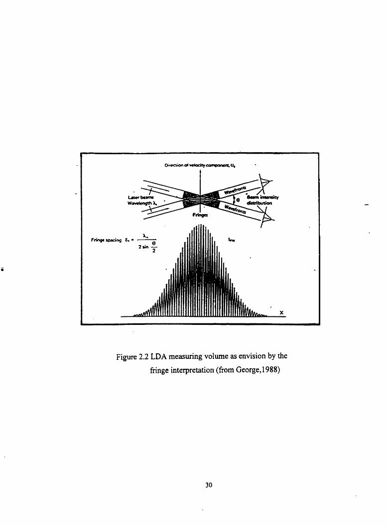
Figure 2.2 LDA measuring volume as envision by the
fnnge interpretation (fiom George, 1988)
Bc ment 1 Volume , B a r n 1
Signal
Figure 2.3 Schematic of the Aerometrics LDA optical configuration
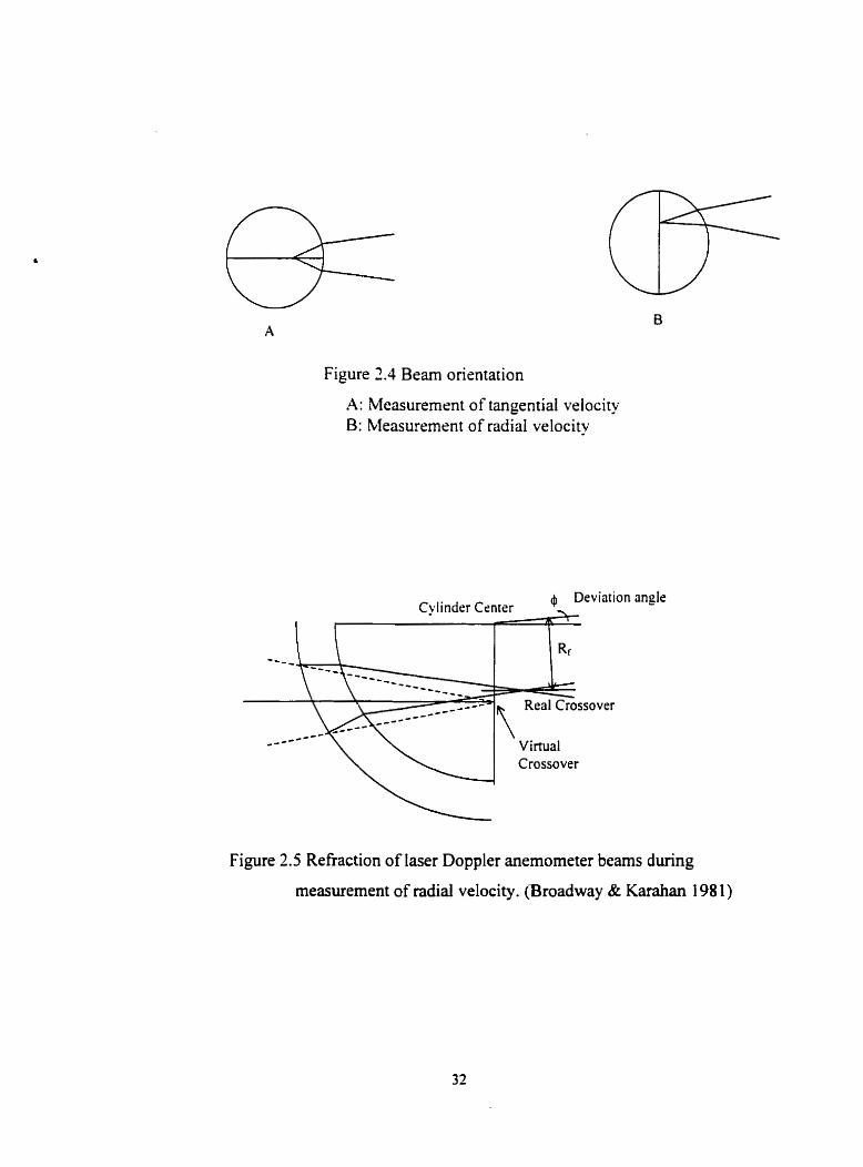
Figure 2.4 Beam orientation
A: Measuremrnt of tangential velociry B: Measurement of radial velocity
Deviation Cvlinder Cenrer
--__ _--- __-- Real Crossover
-c-- \ \ Virtual Crossover
angle
Figure 2.5 Refiaction of laser Doppler anemometer bearns during
measurement of radial velocity. (Broadway & Karahan 198 1)
O 1 a 20 30 4 O 5 0 60 3 O
Radius (mm)
Figure 7.6 Deviation angle in the cone of cyclone when riieasuring
radial ~e loc i ty at z=3OO mm from the bottom
Connected to the
Dry ice
Dry ice level 1 I
Building stearn
main hose
Figure 2.7 Diagram of dry ice
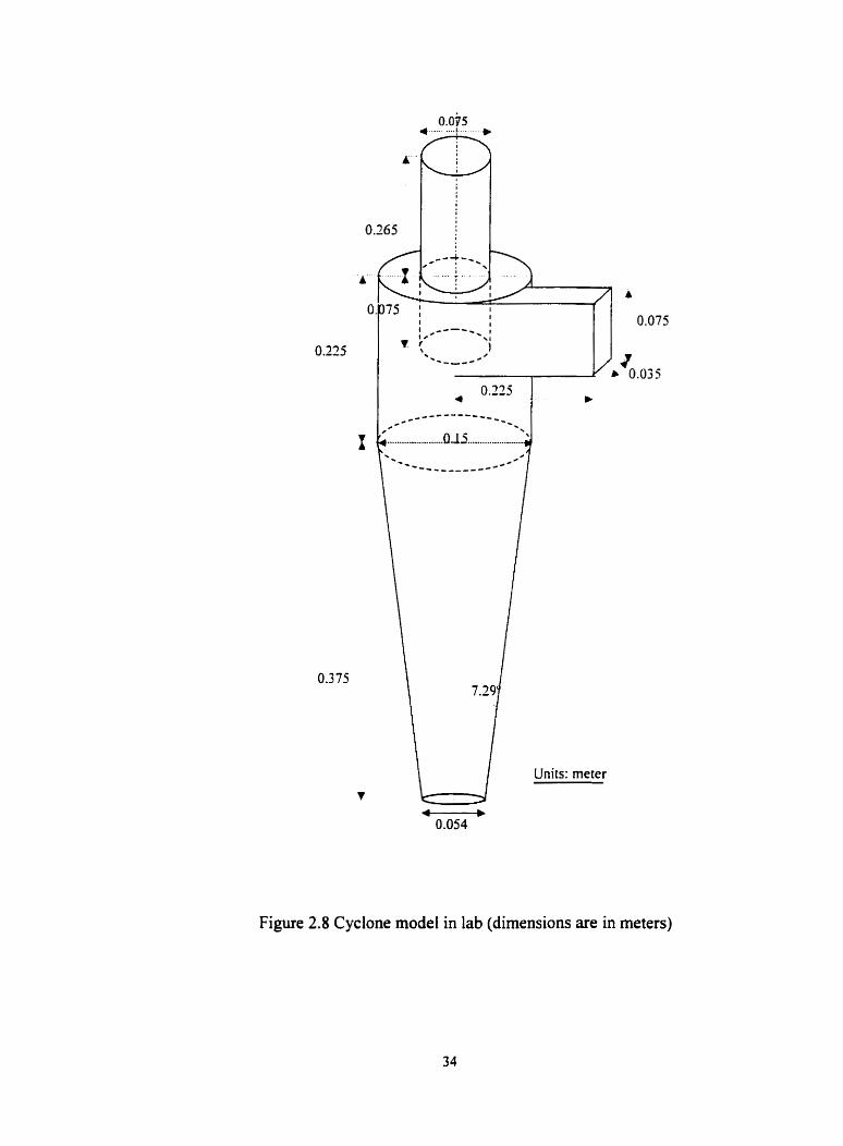
Figure 2.8 Cyclone mode1 in lab (dimensions are in meters)
Seeding in
Figure 2.9 The comection of cyclone inlet to hose
% of the motor full load
Figure 2.10 Repeatability and calibration of the inlet velocity The velocity measurements were taken at d a 4 . 5 and y/b=0.5 . where a and b are the width and height of the inlet
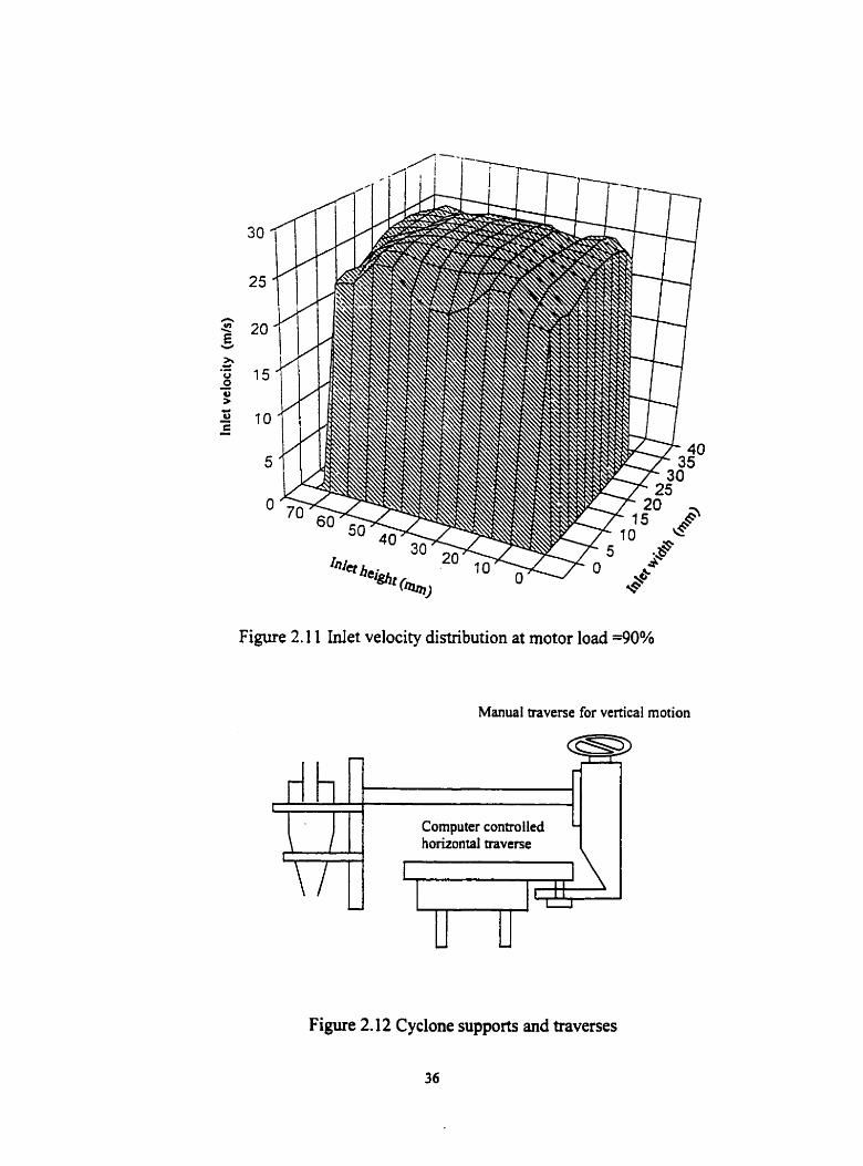
Figure 2.1 1 Met velocity distribution at motor load 4 0 %
Manual traverse for vertical motion
Figure 2.1 2 Cyclone supports and traverses
ri
Cornputer controlled I
horizontal traverse
I -
- -.
Sample size
Figure 2.13 Tangential velocity measurernents with varying sarnple size. Each point in the figure is obtained by averaging values of 3 runs

Reference
Bhonet M., 1 983. Design meihods for aerocyclones and hydrocyclone, C hapter 32 in '* - - - -* . - - .
handbook of Fluids in motion. Ann Arbor science *. - Broadway John D. & Emin Karahan, Correction of laser Doppler anemometer reodings
for refracrion ur cylindrical inierfaces. Disa Information #26. February 198 1
Crane R.I. & M.I. Moore, 1972, Interpretation ofpifot pressure in compressible hvo-
phasefloiv. J.Mech.Eng.Sci. 11.128
Drain L.E.. 1980. The laser Doppler technique. John Wiley and Sons. Toronto
Dring. R. P.. 1987. Sizing criteria for (user. anemornetry parficles. J. Fluids engineering.
104. p15-17
Gardavs ky J.. J.Hrbek. Z.Chara. and MSerera. 1 989. Refnrction correctionsfi>r LDcl
measziremenrs in circulur tzr bes ivithin rrct~ingular opticol boxes. Dantec 1 n format ion.
measurement and anal pis. no.8.
George W.K.. 1988. @tanlirarive measurernent with burst-mode laser Doppler
anemometer. Exptl. Thermal and Fluid Sci. 1,
Hinze J.O. 1 959. Turbulence: an introduction to its mechunism und rheory. McGraw-
Hill . New York
Kresta S. M.. 1 99 1, Characterizarion. mrasirremenf and prediction q f rhe tirrbuient flo w
in stirred tanks. pp28 1 . Ph.D diesis
Kundu, K. Pijush, 1990, Fhid mechanics, Academic press. San Diego. California.
Zhou G., 1996, Characteristics of turbulence rnergy dissipation and liquid-liquid
dispersion in an agitated tanks. Ph.D thesis, University of Alberta, Edmonton. Alberta

Chapter 3: Experimental results
In this chapter, velocity field measurements will be discussed. Before presenting the
esperimental results. the techniques used to analyze the frequency and oscillations in
local velocity are introduced.
3.1 Data analysis technique
In this study. spectral analysis is used to analyze the low frequencies in the velocity field.
The instantaneous veiocity signal of a turbulent tlow c m be interpreted as the surn of a
wide spectnim of frequencies. The relative contributions of the individual frequencies to
the sum are represented by the frequency spectrum or spectral density. The power
spectral density (PSD) and the autocorrelation fùnction provide powerful information for
a physical interpretation of the dominant frequencies and time scales in the flow field.
The PSD gives the enerpy or power content of the signal in a specified frequency band.
The autocorrelation gives a measure of the extent to which a signal correlates with a
displaced version of itself in tirne.
The estimation of frequency spectra from the LDA signal is very important in
determining the frequencies present in turbulent flows and their associated time and
length scales. When the data are evenly spaced. the fast Fourier transfom can be used
directly to process the raw signal to obtain the PSD or autocorrelation function
coefficient. In Our DSA (Doppler signal analyzer), the particles cross the rneasuring
volume at inegular time intervals; hence. the conventional spectral estimates based on
constant sampling rates must be modified. This was achieved using a slotting averaging
technique.
3.1.1 A lias free santpiing
It is well known that the spectrum of a signal c m be obtained unambiguously From equi-
spaced sampled data oniy if the signal has been sampled fast enough. To avoid the
aliasing of high-frequency energy down to lower fiequencies, it is necessary to sample at
a rate equivalent to twice the frequency above which the signal energy content is
negligible. This is generally called the Nyquist criterion (Wills, 1991). In our system, the
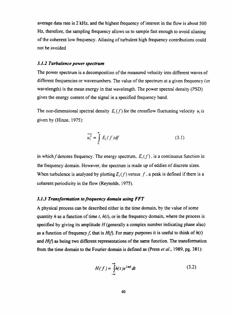
average data rate is 2 kHz, and the highest frequency of interest in the flow is about 500
Hz, therefore, the sampling fiequency allows us to sample fast enough to avoid aliasing
of the coherent low fiequency. Aliasing of turbulent high frequency contributions could
not be avoided
3.1.2 Turbulence power spectrum
The power spectnvn is a decomposition of the measured velocity into different waves of
diverent frequencies or wavenurnben. The value of the spectrum at a piven frequency (or
wavelength) is the mean energy in that wavelength. The power spectral density (PSD)
gives the energy content of the signal in a specified frequency band.
The one-dimensional spectral density E, (f) for the crossflow fluctuating velocity u, is
given by (Hime. 1975):
in which f denotes fiequency. The energy spectmm, E, (/). is a continuous function in
the frequency domain. However, the spectrum is made up of eddies of discrete sizes.
When turbulence is analyzed by plotting E, ( f ) versus f . a peak is defined if there is a
coherent periodicity in the flow (Reynolds. 1975).
3.1.3 Trans formation to frequency domain using FFT
A physical process c m be descnbed either in the time domain, by the value of some
quantity h as a fûnction of time t, h(t), or in the fiequency domain, where the process is
specified by giving its amplitude H (generally a complex number indicating phase also)
as a function of fiequencyf; that is Hm. For many purposes it is useful to think of h( f )
and Hu) as being two different representations of the same function. The transformation
fiom the time domain to the Fourier domain is defined as (Press et al., 1989, pg. 38 1):
where time t is in seconds and fiequencyj'in Hertz.
Computational work using a Fourier transform involves a discrete list of measurements-
h&), rather than a continuous function h(t). Thus. the integral (3.2) in its discrete form is
(Press et. al., 1989):
+a N-I
" d ~ ' d r ~ ~ h k ( r ) e ' 2 " f n r ' ~ l k = ~ ~ h k ( t # 1 2 ' m 1 1 (3.4)
Equation (3.4) is the discrete Fourier transform of iV points hk where k denotes the point
in the time domain and k = O, I. 2. . . . . . .. X 1: n denotes the point in the frequency
domainf, = n / T and n = 1.2. . . . . . .. IV; and Atk = t h - , - t k is the sampling interval.
From equation (3.4). it is obvious that the discrete Fourier transfom (DFT) involves i~'
cornplex muItiplications. This number c m be reduced with an algorithm called the fast
Fourier vansfom (FFT), which involves data reordering by bit reversal order and the
Danielson-Lanczos lemrna. Data are subdivided into N/2 even-nurnbered and iVl2 odd-
numbered points and their discrete Fourier transform is calculated. This subdivision goes
fùrther d o m to 1. Thus bit-reordering data takes N operations, and the discrete Fourier
transform of length 2,4,8.. . N takes log& so that the whole algorithm @es MogiN
operations. For large N, the difference between IV2 and MogzN becomes very significant.
The one-sided power s p e c t m may be calculated as:
when the function h(t) is red, then HV) = H(-j), so that a factor of 2 is expected in the
above equation. Since the quantity involved is not power, but the RMS velocity squared.
the factor of 2 drops out.

3.1.4 Autocorrelation Fmction
The autocorrelation function of physical data establishes the correlation between values
of the data at anytime and values at a future tirne. The autocorrelation function
coefficient RE (or autocorrelation) is calculated fiom the following equation with r the
time delay between the two signals:
The autocorrelation function coefficient has the following relationship:
The general character of the dependence of an autocorrelation coefficient on the time
delay shows zero dope at t = O. This cm be justified as follows: the autocorrelation of a
stationary random hinction of time must be an even function of r . spmetncal about r =
O. Turbulent motions are continuous. with the smallest scales still of finite size; hence
there is a finite delay before the signal changes at d l . and the curve is level at t = 0.
However, in practice. the smallest scales are comparable to or smaller than the transducer
resolution. and it is not possible to see this leveling out.
AAer cornputing the Fourier transfom of the initial time series. the autocorrelation c m be
obtained by multiplying the FFT transform by its complex conjugate:
where H, is discrete Fourier transfonn and Hk* is the complex conjugate of Hk. The
inverse is also true.
3. 1.5 Anoiyzing uneveniy spaced data
For data taken at equi-spaced intervals in time, both the standard fast Fourier transform
(FFT) and the discrete Fourier transform (DFT) can be used to yield spectral estimates. In
this mdy, the FFT algorithm was used in order to Save calculation time. Since the
particle arriva1 times in the LDA data are irregular, the data sets are sampled at random
instants of tirne. The raw data must be reprocessed before the FFT can be applied.
Methods for computing power spectra fiom unevenly sampled data c m be classified into
two categories (Mees 1990): correlation based methods which caiculate the power
spectrum from the Fourier transform of the autocorrelation function, and direct methods
which are based on a direct Fourier transform (DFT) of the data. There are several
methods available to speed up the calculation of spectra from random data for both the
correlation-based methods and the direct transform methods. The best-developed
methods are the 'sloning' methods that qumtize time intervals. This quantization
procedure can be applied either to the amval times of the original sarnples, or,
altematively, to the lag times associated with each pair of data samples. In either case the
quantization results in the crossproducts associated with each pair of data sarnples being
accumulated in 'slots' or 'bins' in the correlation plane. With the autocorrelation function
determined, the FFT is obtained by transform.
In this study, the fast Fourier transform is applied directly to bimed data to calculate the
spectrum. This estimate is fomed by dividing the measurement time into equi-distant
intervals or slots. The LDA data consist of discrete points U ( t , ) at times r , . The bin size
3 was chosen to be at least , or on the average 2 points per bin. The equally
fnteurt - uintp/,ttc
spaced time series is obtained by taking the average of the velocity measurements in each
bin. For empty bins, the value from the previous bin is used. Then. the mean velocity of
al1 the bins is computed and subtracted from the velocity in each bin. giving the time
2 signal a zero mean. Bin sizes of - 4
and - , were also tested. They gave the same /hwI.rt /Slyri.Tl
peak location as before.
Since the new time sequence is expressed in terms of the equi-spaced lag time, an FFT
can be applied directly. In Our study, the power spectnim density was calculated using
Eq. 3.5, while the autocorrelation function was cdculated by applying the inverse Fourier
transform to the product of the Fourier transfomi and its complex conjugate. The slotted

direct method is much faster than the DFT or the binned A/C rnethod for high sampling
rates.
3.2 Flow field measurements
To determine the possible existence and extent of reverse flow, and the transient flow
characteristics, the time varying axial, tangential and radial velocities were measured at
various locations in the cyclone. The axial velocity was measured inside or just outside
the gas outlet tube along the centerline that is perpendicular to the inlet as shown in
Figure 3.1. The radius of the centerline which is near to the inlet is defined as positive
and the other half as negative. Some axial velocity measurements were also carried out in
the cone. Tangenthi velocity measurements were conducted just outside the gas outlet
tube and in the barrel for cornparison with previous investigations. A few radial velocity
measurements were taken just below the vortex finder to determine if there is short-
circuiting in that area. The frequency of any oscillations was determined [rom a
frequency analysis of the velocity time series. Three outlet tube diarneters were used: 50
mm, 75 mm, and 95 mm. giving outlet diameter to barrel diameter ratios of O.3XO.50
and 0.63. The rnajority of the data reported hrre is for the case of Do,rcel/Dbml = 0.50 and
for a rnotor Ioad of 100%.
3.2. l In let velocity
In Chapter 2. the inlet velocity profile and the calibntion of the streamwise velocity in
the centre of the inlet with motor load were discussed. Figure 3.2 shows the streamwise
velocity in the center of the inlet ai three different gas outlet tube diarneters. The
streamwise inlet velocities increase linearly or slightly parabolically with the percentage
of full motor load. The parabolic curve could be due to a pressure drop increase at high
motor loads. It is not surpnsing that the larger the diameter of the gas outlet tube, the
higher the velocities at the sarne motor load. Since with a small gas outlet tube the
pressure drop due to fiction will be higher, the velocity will be reduced based on the
mechanical energy balance. At a low motor load, the pressure drop is relatively low and
is the same for al1 three gas outlet tubes, since pressure drop is proportional to the square
of inlet velocity. Therefore, the discrepancy in streamwise velocities between different
gas outlet tube diameters only exists at high motor loads (Figure 3.2). If we extend the
three lines to the auis. they pass right through the origin, indicating that there is no flow
when the motor is off.
The velocity distributions in the inlet at different motor load and different gas outlet tube
diameters were also measured. Figure 3.3 is representative of the inlet velocity
distribution in the inlet showing h l l y turbulent flow. The superficial velocity at the inlet
was calculated by the following procedure: time varying velocity is averaged at the four
nodes of each rectangular area and is then integnted over this area to get a volumetric
flow rate. A superficial velocity of the inlet is obtained by adding al1 the volumetric flow
IV4 rates from each area and dividing over the inlet area. i.e. " . The streamwise
A,,,
superficial velocities with percentage of full niotor load at different gas outlet diameters
are shown on Figure 3 .J.
Frequency analysis is applied to the inler velocity records for cornparison with the
frequency spectrum of the velocity signals in the gas outlet tube. Figure 3.5 is a time
series plot of the velocity signal at a typical point in the inlet. Figure 3.6 is a power
spectrum plot. The abscissa is the frequency ploned on a logarithrnic scale running from
0.1 to 400Hz. The ordinate is the power spectral estimate plotted on a logarithrnic scale.
The area under the spectmm estimate curve is the variance of the signal and thus
represents the power of the fluctuations. Since there is no discernible peak in the
spectrum. the flow is random. The autocorrelation f ic t ion coefficient on Figure 3.7 does
not show the presence of oscillations around the time axis, revealing that the flow is
purely turbulent. Al1 these indications provide confidence that there is no periodic motion
in the inlet.
3.2.2 Axial velocity
3.2.2.1 Penodic motion detected
The periodic motions in the cyclone were studied using the time varying velocity record
acquired with the LDA. A typical time series of the axial velocity, shown in Figure 3.8,
indicates a very regular penodic motion at 265 Hz. As mentioned before, a power
s p e c t m is the fkequency decomposition of the variance of the signal. A peak in the
power spectnün estirnate represents a coherent fluctuation at that frequency. The distinct
peak in Figure 3.9 confirms that there is periodic motion in the flow field at this
measuring point, leading to a clean oscillation at the same frequency in the corresponding
autocorrelation function plot as shown in Figure 3.10. The data shown in Figure 3.8 - 3.10 were collected 50 mm below the top of the gas outlet tube and 32.5 mm from the
center. Footnote h, denotes the vertical distance from the measuring position to the top
of the gas outlet tube. A positive value of h , indicates that the measuring position is
below the gas outlet tube. while a negative value of h , indicates that the measuring
position is above the gas outlet tube.
The regular oscillation observed in the gas outlet tube is the result of a large-scale
coherent structure. rather than of random turbulent fluctuations. Hussain ( 1986) defined a
coherent structure as follows: A coherent structure is a connected turbulent fluid mass
with instantaneously phase-correlated vorticity over its spatial extent. That is. underiying
the random, three-dimensional vorticity that characterizes turbulence. there is a
component of large-scale vorticity which is instantaneously coherent over the spatial
extent of a coherent structure. As a consequence of this definition. a turbulent flow can be
decomposed into coherent structures and incoherent turbulence. Coherent structures play
important roles in transports of heat, mass and momentum. Simulations have shown that
the coherent structure or precessing vortex core in a cyclone takes on a helical shape
(Mees 1997).
3.2.2.2 Oscillations at h,, = -2 mm, varying r
This vertical position is just above the top of the gas outlet tube. Figure 3.1 1,3.12 and
3.13 show the power spectra for the axial velocity components at three different radial
locations but the sarne vertical position. At r = 30 mm (Figure 3.1 l) , there is one distinct
peak at 260 Hz. At r = 20 mm (Figure 3.12), two peaks at 260 Hz and 5 10 Hz are
noticeable with the peak of fundamental fiequency higher than that for ~ 3 0 m m . At r =
10 mm (Figure 3.13), the two amplitudes are once again a little higher than those at r =
20 mm in Figure 3.12, but the fiequency is preserved. The area under the dominant
fiequency increases progressively as the measuring point moves toward the center. The
larger area under the peak of s p e c t m near the center of the tube indicates that the
oscillations are intense there. As mentioned before, the area under a fiequency spectnim
is equal to the variance or mean square of the fluctuating velocity components in a
frequency range, so the power contained below the peak in the fiequency s p e c t m is the
contribution due to the flow fluctuations. The larger the area, the stronger the flow
fluctuations. Since the spectral intensity scde is logarithmic in this study. it is possible
that a large fraction of the energy contained in the flow fluctuations arises fiom coherent
motions. nie second peak in Figure 3.1 2 and Figure 3.1 3 is a harmonic of the
fundamental frequency.
3.2.2.3 Oscillations at r = 30 mm, varying hW
Figures 3.14 and 3.15 are the time series plots and corresponding spectral analysis of the
velocity fluctuations at r = 30 mm and htOp = - 13 mm (outside the cyclone). Tney show a
periodic motion oscillating at a fundamental frequency of 260 Hz with a broad peak in
the frequency estimate (Figure3.15). Figure 3.16 and 3.17 show the periodic motion at
hW = -2 mm but the same radial location. It is clear that the amplitude of the velocity
fluctuation at hfop = -2 mm (Figure 3.16) is a little smaller than that of h , = - 13 mm
(Figure 3.14). This lower amplitude is consistent with the smaller area of the dominant
peaks in the power spectrum (Figure 3.17 compared with Figure 3.15). Figure (3.18,
3.19), (3.20,3.2 1 ), (3 .22,3 Z ) , and (3.24,3.25) are time series and the corresponding
spectra at hm, = + JOmm, +90mm, + 1 1 Omm, and + 13jmm. From the time series plots
(3.1 8, 3.20,3.22, and 3 .X), the amplitudes of the velocity fluctuations are clearly
decreasing and the energy contained in the fiequency reduces at a rate of at least an order
of magnitude consecutively (3.1 9, 3.2 1,3.23, and 3 .X). The progressive1 y diminishing
amplitude of velocity fluctuations and the decreasing area under the dominant fiequency
as the measurements move d o m the gas outlet tube at the sarne radial position
establishes with a high level of certainty that the strength of the oscillations decays down
the gas outlet tube. It seems that the oscillations vanish at the vertical location of hW =
135 mm (Figure 3.24 and 3.25). This could be due to interaction with the wall which
cause the coherent structure to lose its identity.
3.2.2.4 Averaged axial velocity
Since the flow is time varying, both the mean and fluctuating components of the velocity
components are obtained by averaging over a penod long (larger than 0.5 s) in
cornparison with one cycle tirne (less than 0.0056 s) of the lowest fiequency component
of significant magnitude that is present in the flow (the precessing vortex core). The time
averaged axial velocity and the rms axial velocity profiles at hl,= - 13 mm (top of the
cyclone) are s h o w in Figure 3.26 and 3.27. In Figure 3.26, the mean velocity becomes
negative in the center. indicating that. on the average. back flow exists in that region.
Measurements show that the back flow cm penetrate at least half way down the gas
outlet tube as shown later on Figure 3.32. The magnitude of the mis velocity at this
position (Figure 3.27) is quite high when compared with those at other vertical positions.
indicating that the velocity fluctuations could be mainly due to the coherent structure. It
also shows two regions with high velocity fluctuations. These regions coincide with the
regions of high axial velocity gradients in Figure 3.26. This is expected. since velocity
fluctuations induced by the precessing vortex core will, as a first approximation be
proportional to the velocity gradients in the vortex core. The time-averaged flow appears
to be asymmetric, which may be due to the asymmetry of the single inlet in our
experiment. Note that the measuxing range at this elevation is wider than the diameter of
the gas outlet tube (75mm), since at this position (13 mm above the gas outlet tube), the
flow undergoes a sudden expansion and there is still fluid flow beyond the confines of the
tube diameter,
Figure 3.28 and Figure 3.29 are time averaged axial velocity and the rms axial velocity
profiles at hm,=-2m.m (at the top of the gas outlet tube). They have a similar shape to
Figure 3.26 and 3.27. The difference is that the area under the two peaks of the averaged
axial velocity profile (Figure 3.28) is a little smaller than that of hrOP=-1 3 mm (Figure
3.26). This can cause a significant volumetric flow rate decrease since the two peaks are
near the wall. Although the rms velocity peaks (Figure 3.29) still coincide with the high

axial velocity gradient in Figure 3.28, their values are a little smaller than those at h, = - 13 mm (Figure 3.27). This is an indication of the decay of the oscillation in spite of the
fact that the coherent structures are still energetic and dominant at this position (Figure
3.11 -3.13)
In the gas outlet tube at a vertical position of h , = 90 mm, the back flow region in Figure
3.30 has almost disappeared (one point indicating back flow), showing the downward
mass flow rate is less than higher up in the gas outlet tube. The rms velocity profile,
instrad of showing two local peaks, is almost tlat and randomly scattered in the center
(Figure3.3 l), and the magnitude of the rms velocity is much less than that at the top of
gas outlet tube. The rms velocity trend at this location is the same as reported by Boysan
et aL(1983). One hypothesis to explain this variation is that both random and organized
fluctuations contribute comparably to the measured m s velocity fluctuations.
At a vertical position of 135 mm from the $as outlet top. the time averaged axial velocity
is shown in Figure 3.32. The r m s velocity shows one peak at the center (Figure 3.33).
This may indicate that the rms velocity at this elevation is mainly due to turbulent
fluctuations. The decrease of the average rms velocity down the gas outlet tube is another
confirmation of the decay of the oscillation. The values of averaged rms velocities at
different elevations are shown in Table 3.1.
3.2.3 Tangential velocity
The tangential velocity was measured in the barre1 at 0.41 5 m from the top of $as outlet
tube (0.15 m from the cyclone roof). It shows the expected Rankine vortex shape
(combination of a free vortex and a forced vortex) in Figure 3.34. The velocities
measured in this work show the region of solid body rotation persisting much further out
towards the cyclone wall than that reported by Boysan and CO-workers (Boysan et al.
1983) at the same superficial gas velocity. The discrepancy could be due to the 75%
scaling of our cyclone geometry dimensions. It can also contribute to the conservation of
angular momennim. With a smailer diarneter cyclone at the same iniet velocity, the
tangential velocity has to increase to maintain the same angular momentum. This could
cause a shifiing of the maximum tangential velocity towards the wail.
3 .2.3.l Oscillations in tangential velocity
Frequency analysis was applied to tangential velocity time senes to veriS, the fiequency
of the oscillations. Figure 3.35, 3.36 and 3.37 are ploned at a selected point just outside
the gas outlet tube. The time series record shows vigorous periodic motion on Figure
3.35, the frequency spectrum (Figure 3.36) and autocorrelation function coeficient
(Figure 3.37) indicate that the periodic motion has a fundamental frequency of about 260
Hz, identical to the oscillation frequency of the axial velocity fluctuation. The fact that
the axial and tangential oscillation frrquencies are the same confirms that the oscillations
are caused by a coherent structure.
3.2.3.2 Oscillation darnping in the barrel
Frequency analysis was also applied to the tangential velocity record in the barrel (Figure
3.38). No noticeable peaks are observed (as shown in Figure 3.39). although some
irregular low frequency oscillations seem to be present in the time series record (Figure
3.38) and autocorrelation function (Figure 3.40). 11 is clear that periodic motions are
greatly darnped out in the barrel, if they exisr at all. For a DOu,/JDbm, ratio of 0.63, one
broad peak c m be observed in the frequency spectrum (Figure 3.4 1 ) although the
coherent fluctuations revealed by the power spectnun was much less energetic (the PSD
only reaches to 106) and only contain a modest proportion of the power contained in the
flow fluctuations. For a Dowir/Dbarrer ratio of 0.53. the frequency spectrum does not show
any distinct peaks (Figure 3.42).
3.2.3.3 Oscillations in the cone
To test if there are oscillations in the cone, a large number of runs were camed out in the
cone (1 80 runs). A representative spectnim is presented in Figure 3.43. No peak of any
significant magnitude cm be detected. The autocorrelation fùnction (Figure 3.44) looks
like a combination of several dominant frequencies, indicating that the flow fluctuations
could be more randorn. The velocity fluctuations in the cone with the other two gas outlet
tube diameters yield similar spectra to this one.
3.24 Measurements ut d i f j en t inid velocities
B y setting the percentage of the full motor load on the motor drive, the inlet velocity c m
be changed. Figure 3.45.3.16 and 3.47 show the continued existence of periodic motion
in the flow field at a motor load of 50% (Le. at about 13 m/s superficial inlet velocity). At
this inlet velocity the oscillation has a fundamental frequency of 130 Hz. Experiments
show that the frequency of the oscillations scales linearly with the superficiai velocity of
the inlet for al1 the three gas outlet tube diameters as shown in Figure 3.48. The different
symbols along the regression lines denote different rum. If the lines are extended to zero
frequency, they do not pass through the ongin. This suggests that the coherent structure is
lost at sorne point in the transition to laminar flow. The dimensionless frequency c m be
characterized using the Süouhal number. and it is a function of both Reynolds number
and Swirl number. This will be discussed in detail in the dirnensionless group analysis in
the next chapter. Similar phenornena were also observed for the other two pas outlet
tubes.
3.2.5 Measurements ai different gus ouilet tube diorneters
Changing the outlet tube diameter greatly changes the frequency of the oscillations. Fig
3.49 s h o w that the frequency of oscillation at a selected point just outside the gas outlet
tube with a D,, JDhml ratio of 0.33 is about 490 Hz. The time averaged mean and m s
axial velocities at Zmm above the gas outlet for this ratio are shown on Figure 3.50 and
3.5 1. Figure 3.50 shows similarity with Figure 3.28. but the back flow region is slightly
narrower. Experiments indicated that the back flow and oscillations only penetrate down
to about 113 of the gas outlet tube. The shape of the rms velocity profile in Figure 3.5 1 is
a linle different from Figure 3.29. Near the wall. the rms velocities become higher. This
may be because turbulence energy generation is higher near the wall.
The frequency of oscillation drops to 180 Hz when the diameter-barre1 ratio is increased
to 0.63 as shown in Figure 3.52. A possible explanation for the decrease of oscillation
fiequency with increasing gas outlet tube diameter is that when the passage narrows, the
fiequency of oscillation must increase in order to preserve the anguiar momentun of the
vortex core. and vice versa. The time averaged axial and mis axial velocities (Figure 3.53

and Figure 3.54) show the same trends as those of the small gas outlet tube. Our
experiments also show that the back flow c m penetrate to the roof of the gas outlet tube
of this gas outlet tube diameter.
Changing the diameter of gas outle: tube will change the swirl in the cyclone: this will be
discussed in detail in the next chapter.
3.3 Discussion
3.3.1 The mechankm of back jhw
As mentioned in Chapter 1, back flow or reverse flow is a well known phenornenon in
highly swirling flow. In order to analyze the reverse flow using the Navier-Stokes
equations. imposing mi-symmetry is unfortunatel y necessary. By doing so. the continuity
equation can be expressed as:
in which v is the radial velocity and u is the axial velocity.
The energy equation is given by:
in which the term in square bracket on the right hand side denotes viscous dissipation.
a-4 E, =- (3.1 O) az
equation 3.10 is viscous dissipation of swirl component on the axial direction when
assuming B independent.
and equation 3.1 1 is the vorticity component in the r direction.
In swirling flows, axial gradients are much smaller than radial gradients, so that the
interaction of the pressure and the swirl may be exarnined using the quasi-cylindrical
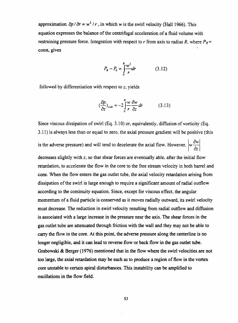
approximation ap l a>. = w 2 l r , in which w is the swirl velocity (Hall 1966). This
equation expresses the balance of the centrifugai acceleration of a fluid volume with
restraining pressure force. htegration with respect to r fiom axis to radius R, where PR =
const, gives
followed by differentiation with respecr to z, yieids
Since viscous dissipation of swirl (Eq. 3.10) or. equivalently. diffusion of vorticity (Eq.
3.1 1) is always less than or equal to zero, the axial pressure gradient will be positive (this
is the adverse pressure) and will tend to decelerate the mial flow. However. iv- I :l decreases slightly with z, so that shear forces are eventually able. afler the initial flow
retardation, to accelerate the flow in the core to the free Stream velocity in both barre1 and
cone. When the flow enters the gas outlet tube, the axial velocity retardation arising fiom
dissipation of the swirl is large enough to require a significant amount of radial outflow
according to the continuity equation. Since, except for viscous effect. the angular
momentum of a fluid particle is conserved as it rnoves radially outward, its swirl velocity
must decrease. The reduction in swirl velocity resulting fiom radial outflow and difision
is associated with a large increase in the pressure near the a i s . The shear forces in the
gas outlet tube are attenuated through friction with the wall and they may not be able to
carry the flow in the core. At this point, the adverse pressure dong the centerline is no
longer negligible, and it can lead to reverse 80w or back flow in the gas outlet tube.
Grabowski & Berger (1976) mentioned that in the flow where the swirl velocities are not
too large, the axial retardation may be such as to produce a region of flow in the vortex
core unstable to certain spiral disturbances. This instability c m be arnplified to
oscilIations in the flow field.
Since we believe the dominant factor causing reverse flow to be the decline of swirl
velocity in the gas outlet tube, it is possible to explain that the back flow c m occur nearer
to the top with a smaller gas outlet tube. In this case, due to angular momentum
conservation through barre1 to the gas outlet tube, the swirl velocity has to increase more
in a small gas outlet tube to some extent. Therefore it may compensate the swirl loss
which is caused by radial outfiow so that the back tlow m q occur at a later stage.
3.3.2 Origin of coh erent structure and asymmetric flo w jiled
For decades. people have tried to determine the origin of oscillations in highly swirling
flows. Clark et aL(1990) stated that the coherent structures originate from the upstream
boundary due to the interaction between different sizes of eddies. or due to the interaction
between the eddies with the boundaries. They seem to retain much of their shape and
character as they convect downstream. but eventually die out. Faler &Leibovich (1 977)
found that the increase of swirl will move the axial location of the oscillations upstream.
In Our case, the experimental results show that the coherent structures are the strongest at
the top within the range of measurements. this rnay indicate that they are generated at the
top somewhere, i.e. far downstream, which contradicts most of the phenornena observed
in the literature. Squire(l960) applied wave theories to explain these structures which are
generated downstreams. From his experiment he concluded that waves rnay propagate
upstream from a downstream disturbance source (e.g. created by the tube exit). This
seems to be the case in our study.
In this research, an unsteady three-dimensional asymmetric flow field has also been
observed. Due to the single inlet of the cyclone, it is difficult to decide whether the
asymmeâric geometry or the oscillations contribute to the asymmetric flow field.
Leibovich (1984) stated that flows which suffer breakdown can be made to have a high
degree of axial symmetry, yet the flows in the breakdown zone lose syrnmetry.
The volumetric flow rate Q is defined as follows when assuming axi-symmetric flow:
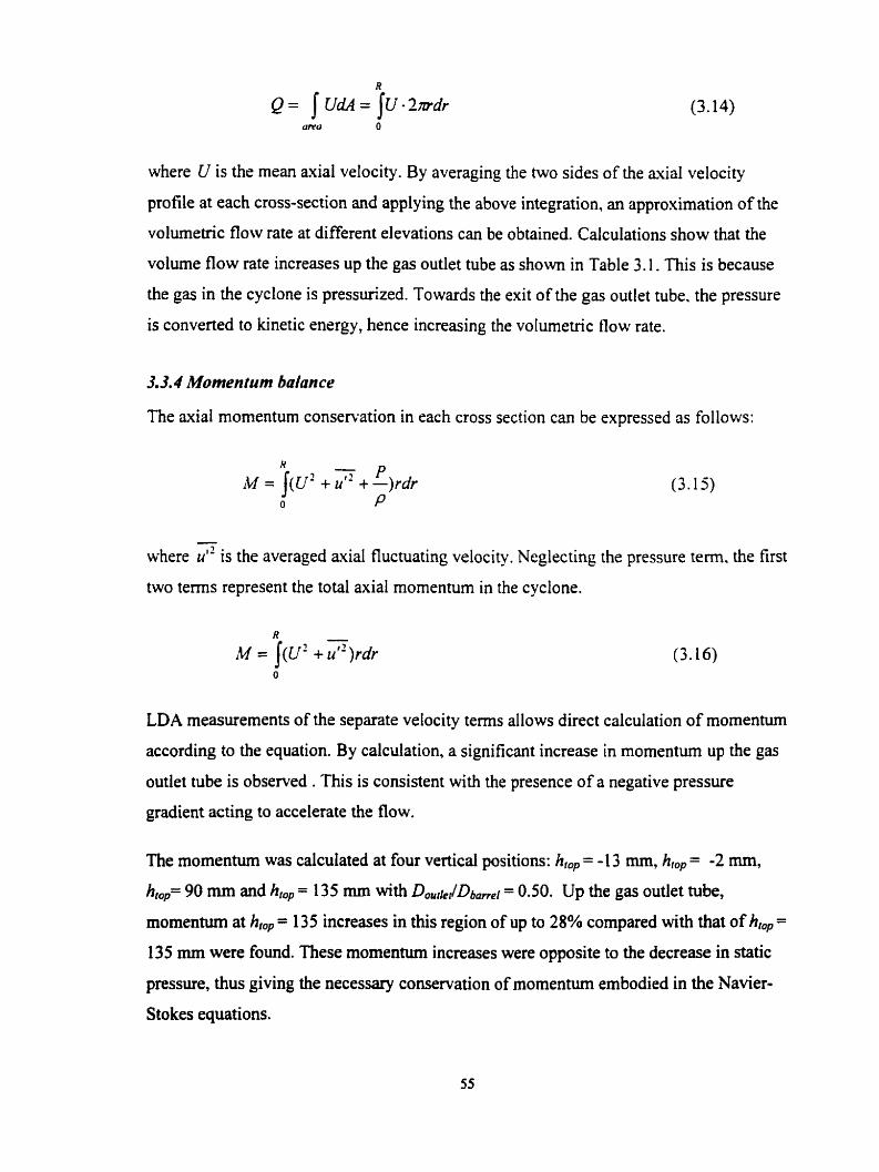
where II is the mean axial velocity. By averaging the two sides of the axial velocity
profile at each cross-section and applying the above integration, an approximation of the
volurnetric fiow rate at different elevations can be obtained. Calculations show that the
volume flow rate increases up the gas outlet tube as s h o w in Table 3.1. This is because
the gas in the cyclone is p r e s ~ ~ z e d . Towards the exit of the gas outlet tube. the pressure
is converted to kinetic energy, hence increasing the volumetric fiow rate.
3.3.4 Momentum balance
The axial momentum conservation in rach cross section c m be expressed as follows:
- where u'' is the averaged axial fluctuating velocity. Neglecting the pressure term. the first
two terms represent the total axial momentum in the cyclone.
LDA measurements of the separate velocity terms allows direct calculation of rnomenturn
according to the equation. By calculation, a significant increase in momentum up the gas
outlet tube is observed . This is consistent with the presence of a negative pressure
gradient acting to accelerate the 80w.
The mornenturn was calculated at four vertical positions: hW = -1 3 mm, h,op = -2 mm,
hm,= 90 mm and htop = 135 mm with Douhi/Db017eI = 0.50. Up the gas outlet tube,
rnomentum at h , = 13 5 increases in this region of up to 28% compared with that of hW =
135 mm were found. These momentum increases were opposite to the decrease in static
pressure, thus giving the necessary conservation of momentum embodied in the Navier-
Stokes equations.

It is of interest to note that at h , = -1 3 mm, the momentum carried by the mean motion
(tirst component of momentum integral in Eq. (3.16)) is 2.7 times that carried by the
streamwise fluctuations. On the other hand, at hm, = 135 mm, the momentum of the mean
motion is 30 t h e s that of the turbulence contribution. This is because most of the
momentum associated with the fluctuation term is in the periodic component (precessing
vortex core), which dominates the fiow at the top but has decayed to almost negligible
levels down the gas outlet tube. Thus, momentum increase due to the pressure effects and
significant transfer of momentum takes place from the periodic component to the mean
flow in the gas outlet tube.
3.4 Conclusions
A detailed experimental investigation was carried out to detemine the effects of inlet
velocity and giis outlet diarneter on the back flow and coherent large-scale oscillations
observcd in the flow field. The results have shown the existence of a well-detined.
energetic low-frequency oscillations (precessing vortex core) and reverse flow for 311 gas
outlet tube diameters to barre1 diameter ratios tested (0.33, 0.50 and 0.63).
Frequency spectra and autocorrelation functions show that at a given velocity. the
oscillating frequency does not depend on the measurement location. In al1 three-diameter
gas outlet tubes. the back flow and oscillation decayed down the gas outlet tube. The
fiequency of the oscillations is dependent on the flow rate and the diameter ratio
Do,ru,/Db,,,~. For dl gas outiet tube diameters, the oscillations were observed over a wide
range of velocities with a fiequency that scales linearly or slightly parabolically with the
inlet flowrate.
The oscillations contribute significantly to the high fluctuation levels at the top of the gas
outlet tube. They may derive their energy from a fluid dynamic instability and originate
at the top of the gas outlet tube. The fluctuation magnitudes Vary considerably in the gas
outlet tube. At the top, they are intense and dominate the flow, while down the gas outlet,
they are negligibly srnall. The two peaks of axial fluctuating velocity are in agreement
with the steepest velocity gradient in the averaged axial velocity.
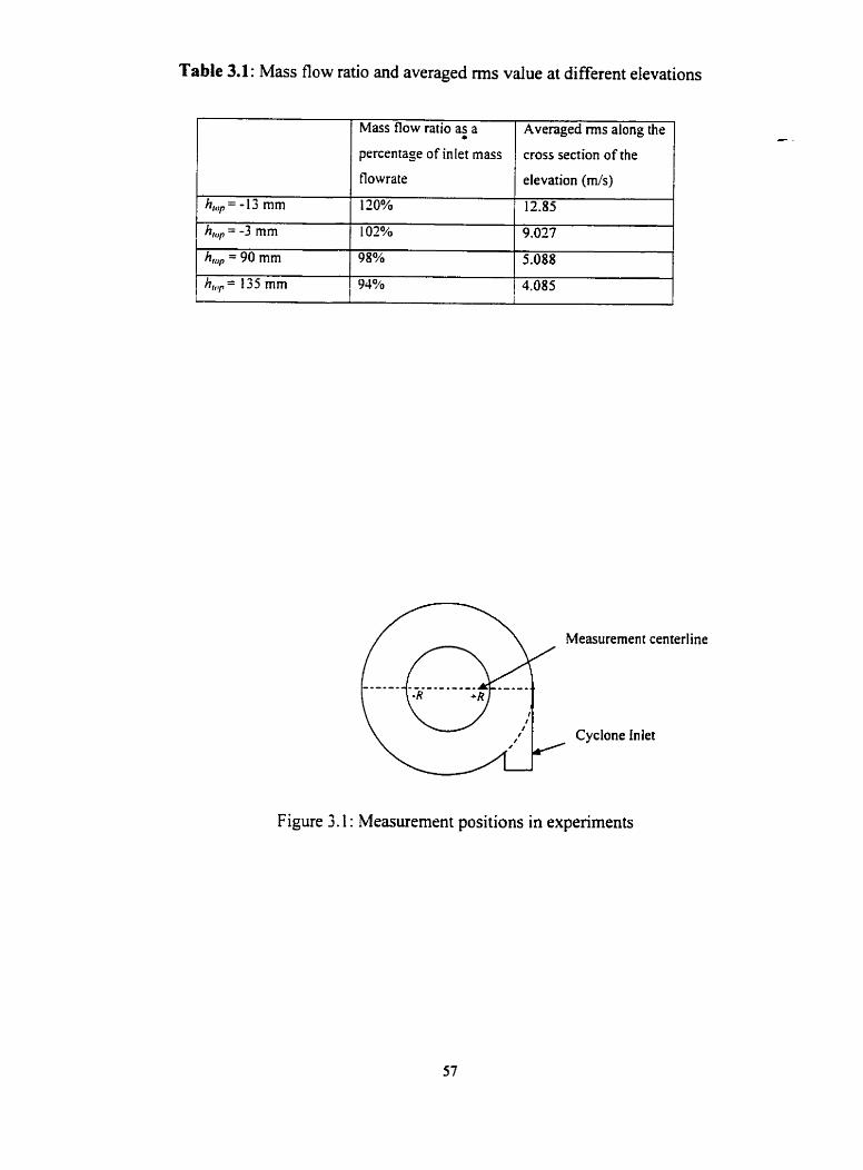
Table 3.1: Mass flow ratio and averaged rms value at different elevations
Figure 3.1 : Measurement positions in experiments
h,,= -13 mm
h,, = -3 mm
h,, = 90 mm
1 h,,,p= 135 mm I
Mass flow ntio % a
percentage of inlet mass
flowrate
t 20%
102%
98%
940'0
Averaged rms along the
cross section of the
elevation (mh)
12.85
9.027
5.088
4.085

with D,,,dDbmC,=0.63
regression O with DoUt,dD,am,,=0.50
regression r with Do ut,c JDb,,=0.33
regression
% of hl1 motor load
Figure 3.2 Repeatability and calibration of inlet velocity for different diameter of gas outlet tube. The velocity measurernents were taken at x/a=0.5 and y k 0 . 5 , where a and b are the width and height of the idet
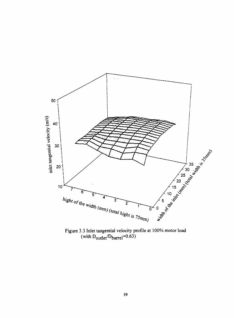
Figure 3.3 Inlet tangentiai velocity profile at 100% motor load (with Do~etmbarre~'o-63 )
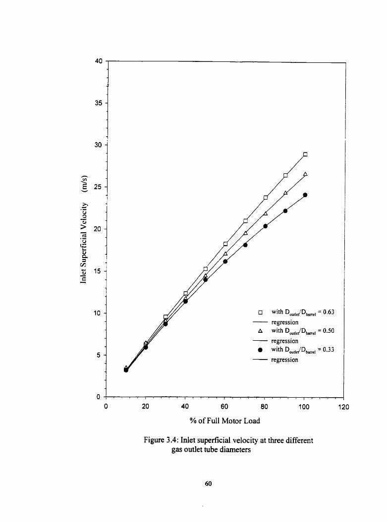
O with Diiutlct/Dborrcl
regression
A with Doutlc(Dbarrel - regression
with ",",,,~Db,, - regression
O 20 40 60 80 1 O0 120
% of Full Motor Load
Figure 3.4: Inlet superficial velocity at three different gas outlet tube diameters

2.2 2.4 2.6 2.8 3.0 3.2 Time (s)
Figure 3.5: Time senes of tangential velocity in cyclone inlet at x/a = 0.33 andylb = 0.4 (with D,,,l,,/Dh,, = 0.50: a and b are the width and height of the inlet)
1 O-' 1 O0 1 O' 1 02 Log (Frequency) (Hz)
Figure 3.6: Frequency analysis in cyclone inlet at .du = 0.33 and y!b = 0.4 (with D,,,,l,(Db,,, = 0.50: a and h are the width and height of the inlet)
0.00 0.05 0.10 0.15 0.20 Time Lag (s)
Figure 3.7: Autocorrelation coefficient in cyclone inlet at xla = 0.33 and ylb = 0.40 (with D,,,JD,,, = 0.50; a and b are the width and height of the inlet)
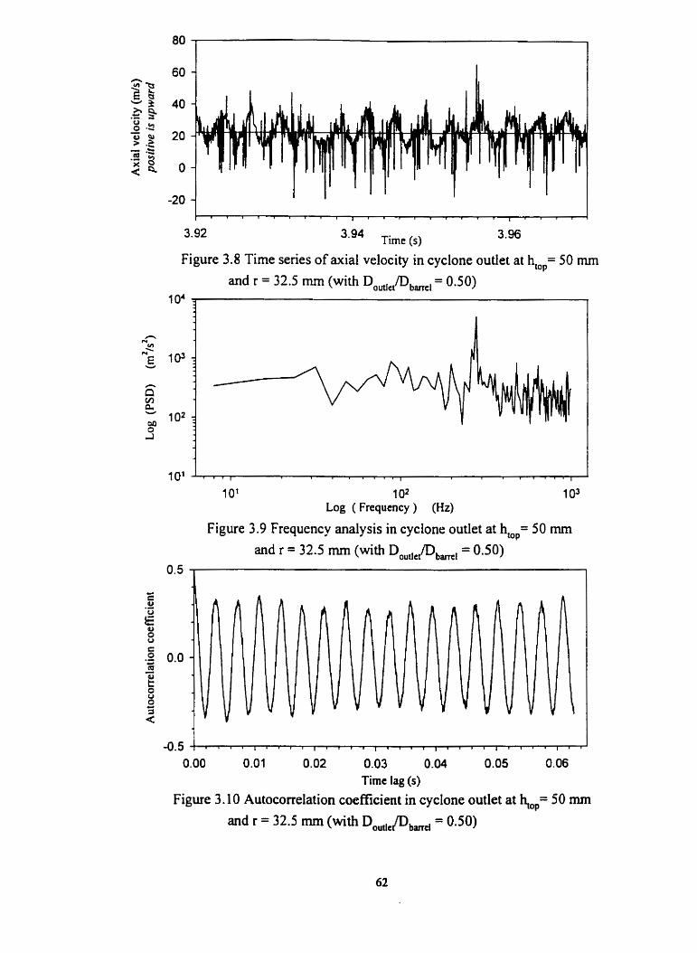
3.94 Time (s)
Figure 3.8 Time series of axial velocity in cyclone outlet at htop= 50 mm
and r = 32.5 mm (with Doutlel/Dbsml = 0.50) 1 O*
1 O2 Log ( Frequency ) (Hz)
Figure 3.9 Frequency analysis in cyclone outlet at hm,= 50 mm
and r = 32.5 mm (with Do,,iin/Db,l = 0.50) 0.5 1
0.00 0.01 0.02 0.03 0.04 0.05 0.06 Time lag (s)
Figure 3.10 Autocorrelation coefficient in cyclone outlet at JOp= 50 mm
and r = 32.5 mm (with D ,,,, Pb,,, = 0.50)

Log (Frequency) (Hz)
Figure 3.1 1 : Frequency analysis at the top of cyclone outlet at h,, = - 2 mm and r = 30 mm (with D ,,,,, (D,,, = 0.50)

Log (Frequcncy) (Hz)
Figure 3.12: Frequency analysis at the top of cyclone outlet at hm, = - 2 mm and r = 2 0 mm (w&D ,,,,,, /D,,,= 0.50)
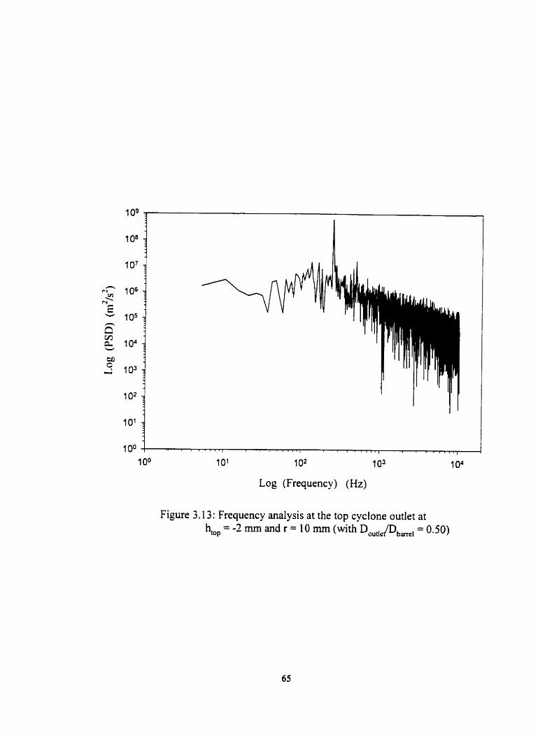
Log (Frequency) (Hz)
Figure 3.13: Frequency analysis at the top cyclone outiet at hlo, = -2 mm and r = 10 mm (with D ,,,,, Pb,, = 0.50)

Tirne (s)
Fig. 3.14 Time series of axial velocity at the top of cyclone outlet at hrop = - 13 mm and r = 30 mm (with D ci/D = 0.50)
Log (Frequency) (Hz)
Fig. 3.15: Frequency analysis of axial velocity at the top cyclone outlet - -
at htop = -13 mm and r = 30 mm (with D ,,,,, Pb,, = 0.50)
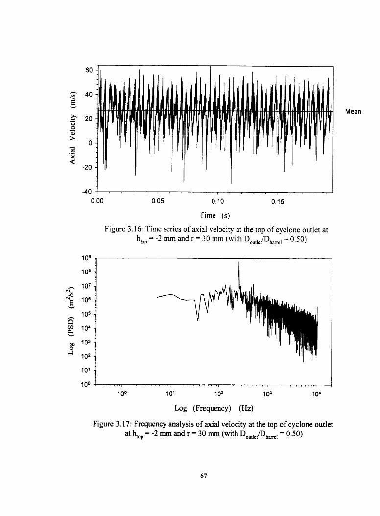
Time (s)
Figure 3.16: Time series of axial velocity at the top of cyclone outlet at hm, = -2 mm and r = 30 mm (with D ,,,,, JD ,,,, = 0.50)
Log (Frequency) (Hz)
Figure 3.1 7: Frequency analysis of axial velocity at the top of cyclone outlet at 4op=-2 mm andr = 30 rnrn(with D,,,,~/D,,, = 0.50)

Time (s)
Figure 3.18: Time senes of axial velocity in cyclone outlet at h,,, = 40 mm
and r = 30 mm (with D,,fl,,/Dbmel = 0.50)
Log (Frequency) (Hz) Figure 3.19: Frequency anaiysis of axial velocity outlet at hl,, = 40 mm
and r = 30 mm (with D,,i,t/Db,l = 0.50)

Time (s)
Figure 3.20: Time series of axial velocity in cyclone outlet at hm, = 90 mm
and r = 30 mm (with DouiieiiD,,,, = 0.50)
Log (Frequency) (Hz)
Figure 3.2 1 : Frequency analysis of axial velocity in cyclone outlet at 4,, = 90 mm and r = 30 mm (with DOutie(D,,, = 0.50)
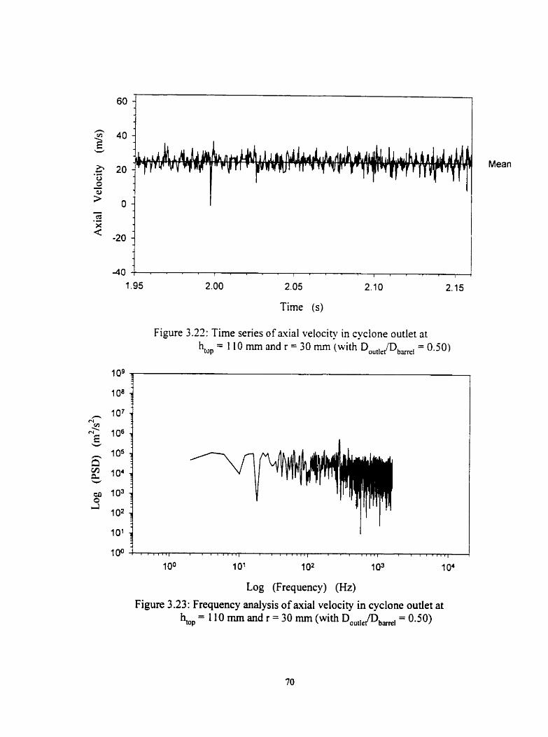
Time (s)
Figure 3.22: Time series of axial velocity in cyclone outlet at h,,, = 110 mm and r = 30 mm (with DoUiic(D ,,,, = 0.50)
Log (Frequency) (Hz) Figure 3.23 : Frequency analysis of axial velocity in cyclone outlet at
hl, = 1 10 mm and r = 30 mm (with DOYiie(Db,, = 0.50)
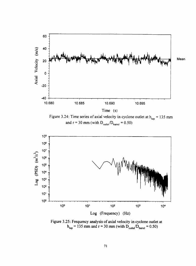
Time (s)
Figure 3.24: Time series of axial velocity in cyclone outlet at hmp = 135 mm
and r = 30 mm (with D,,,l,,/Db,,, = 0.50)
Log (Frequency) (Hz)
Figure 3.25: Frequency analysis of axial velocity in cyclone outlet at hiop = 135 mm and r = 30 mm (with D,ud,(Db,l = 0.50)

-10 - T T 7 1 . 1 < , r . . . , , , , , . , ,
-4 O -20 O 20 40
Radial Distance (mm)
Figure 3.76: Axial velocity profile 13 mm above the top of cyclone outlet tube (with DUUiiel/Dbme, = 0.50)
-40 -20 O 20 40 Radial Distance (mm)
Figure 3.27: The axial rms velocity profile 13mm above the top of cyclone outlet tube (with = 0.50)
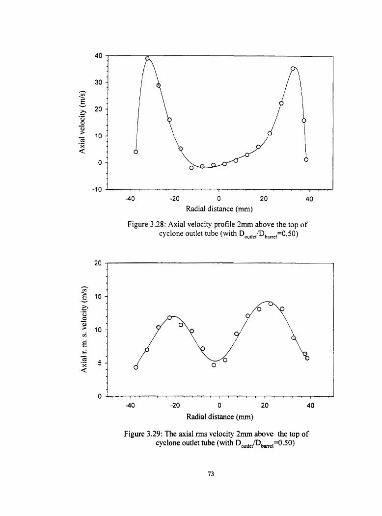
Radial distance (mm)
Figure 3.78: Axial velocity profile 2mm above the top of cyclone outlet tube (with D ,,,,, ,'D =0.50)
Radial distance (mm)
Figure 3.29: The axial rms velocity 2mm above the top of cyclone outlet tube (with D ,,,, ID,,,=O.SO)
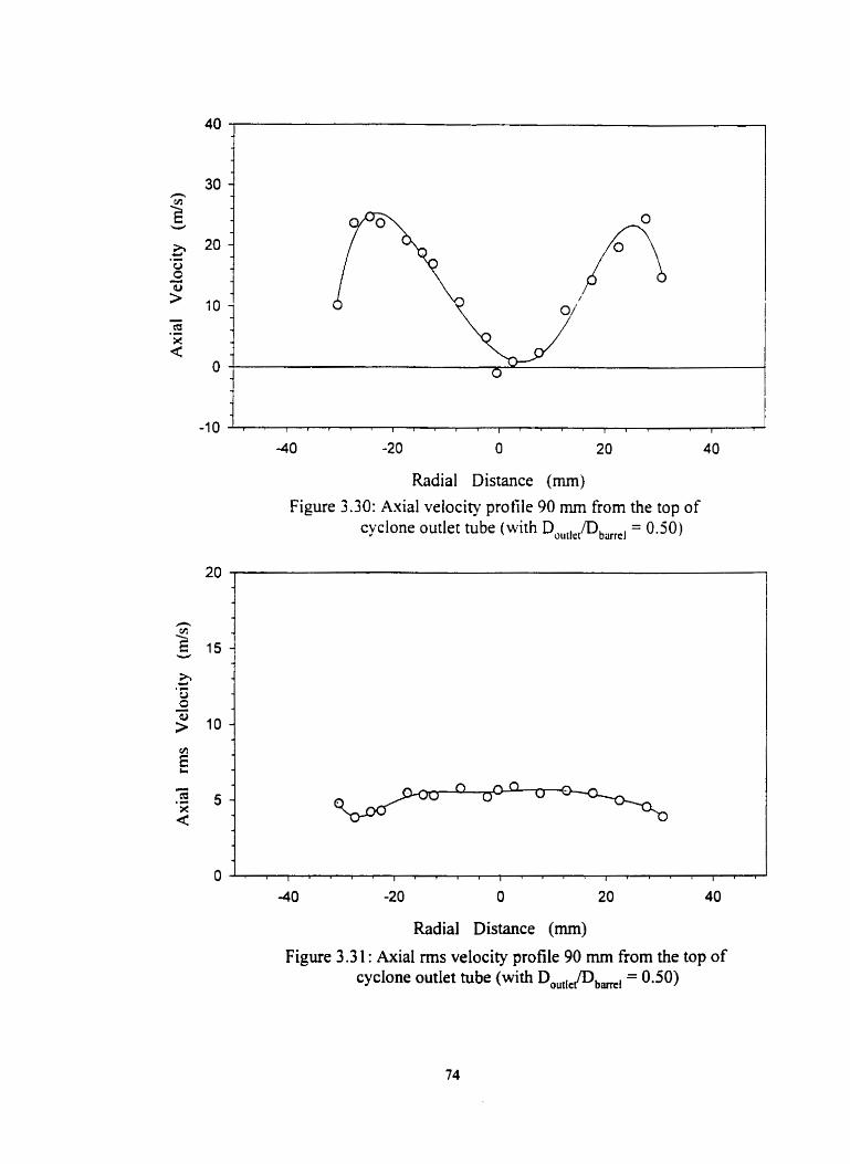
Radial Distance (mm) Figure 3.30: Axial velocity protile 90 mm from the top of
cyclone outlet tube (with D ,,,,, JD ,,,,, = 0.50)
Radial Distance (mm)
Figure 3.3 1 : Axial rms velocity profile 90 mm fiom the top of cyclone outlet tube (with D,,,Ie(D,,, = 0.50)
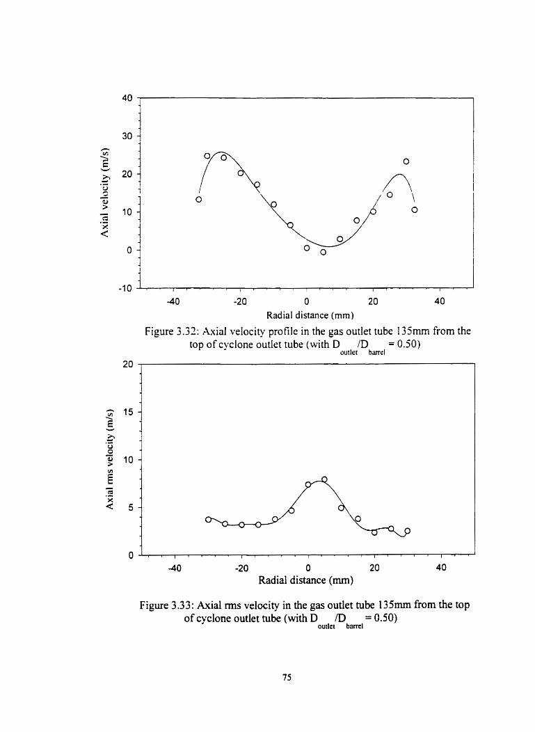
Radial distance (mm)
Figure 3.32: Axial velocity profile in the gas outlei tube 135mrn from the top of cyclone outlet tube (with D iD = 0.50)
outlct bmrl
Figure 3.33: Axial rms velocity in the gas outlet tube 135mm from the top of cyclone outlet tube (with D /D = 0.50)
ouilet barre1
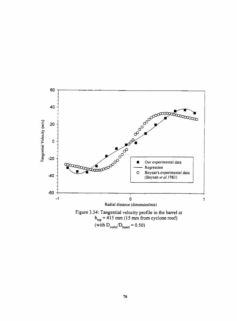
O Boysan's experimental data
I (Boysan et ai. 1983) I
O Radial distance (dirnensionless)
Figure 3.34: Tangential velocity profile in the barre1 at h,,, = 4 15 mm (1 5 mm from cyclone roof)
(with DouiieilDbml = o.50)
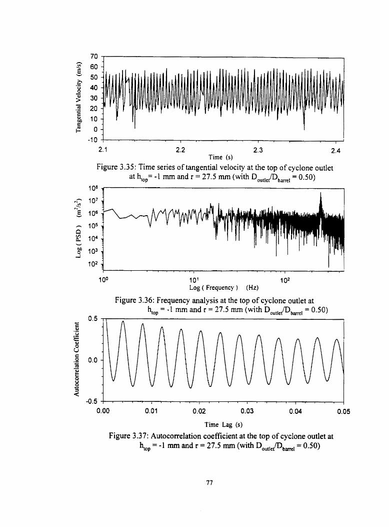
-1 O 1 I 1 I I
2.1 2.2 2.3 2.4 Time (s)
Figure 3.35: Time series of tangential velocity at the top of cyclone outlet at hiop= - 1 mm and r = 27.5 mm (with D,,,l,JDb,, = 0.50)
l o a 1
1 O' 1 o2 Log ( Frequency ) (Hz)
Figure 3.36: Frequency analysis at the top of cyclone outlet at hto, = -1 mm and r = 27.5 mm (with D,,,,,(DbmI = 0.50)
O. 5
0.0
Time Lag (s)
Figure 3.37: Autocorrelation coefficient at the top of cyclone outlet at h,, =-1 mm and r = 27.5 mm (with Do,,&,, = 0.50)
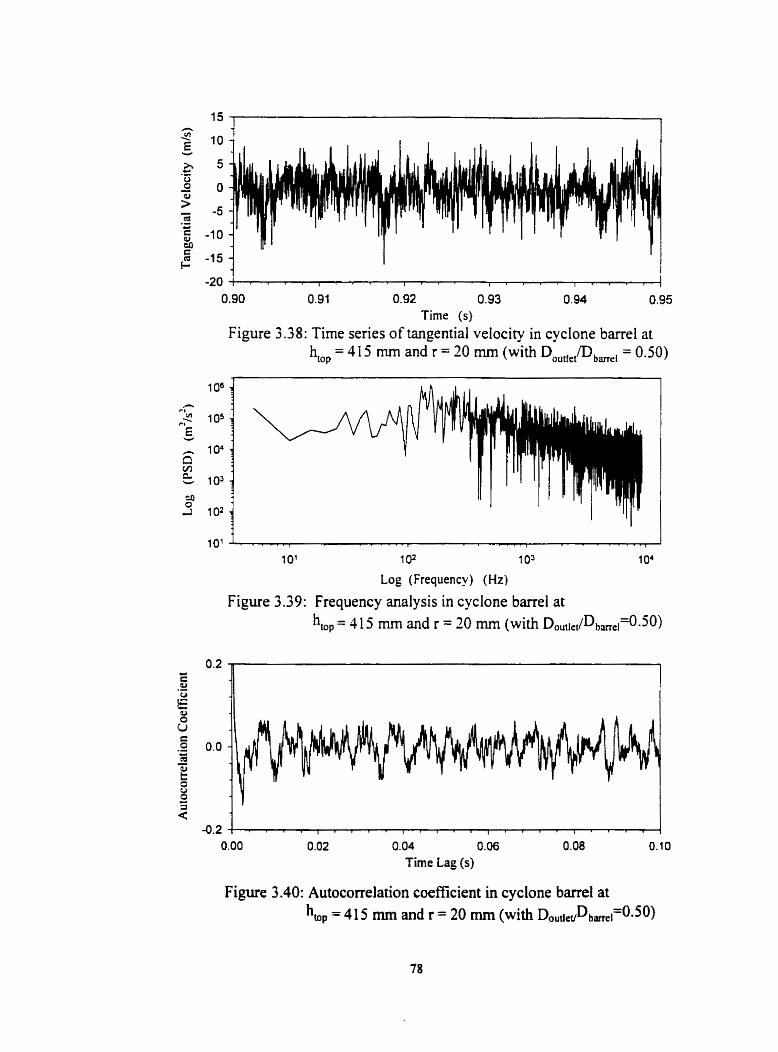
- 2 0 i r 1 . - 1 . . . , 1 , u , , , , , . , , , , , s [
0.90 0.91 0.92 0.93 0.94 0.95 Time (s)
Figure 3.38: Time series of tangential velocity in cyclone barre1 at htop = 415 mm and r = 20 mm (with D a u i i e ~ b m e l = 0.50)
10' l . . . . * , I I r
1 o1 1 oz 1 O= 1 o4 Log (Frequency) (Hz)
Figure 3.39: Frequency analysis in cyclone barre1 at
Q . 2 ! . . . . . . . . . . . . . . . . . . . . . . . . 0.00 0.02 0.04 0.06 0.08 0.10
Tirne Lag (s)
Figure 3.40: Autocorrelation coefficient in cyclone barre1 at = 41 5 mm and r = 20 mm (with ~,.~.yDb,~=O*50)
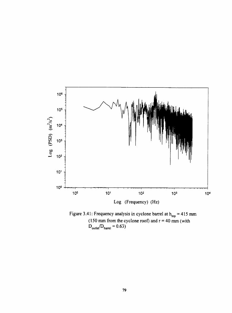
Log (Frequency) (Hz)
Figure 3.4 1 : Frequency analysis in cyclone barre1 at h,,, = 4 15 mm ( 1 50 mm from the cyclone roof) and r = 40 mm (with
D,u*,ePb,, = 0.63)
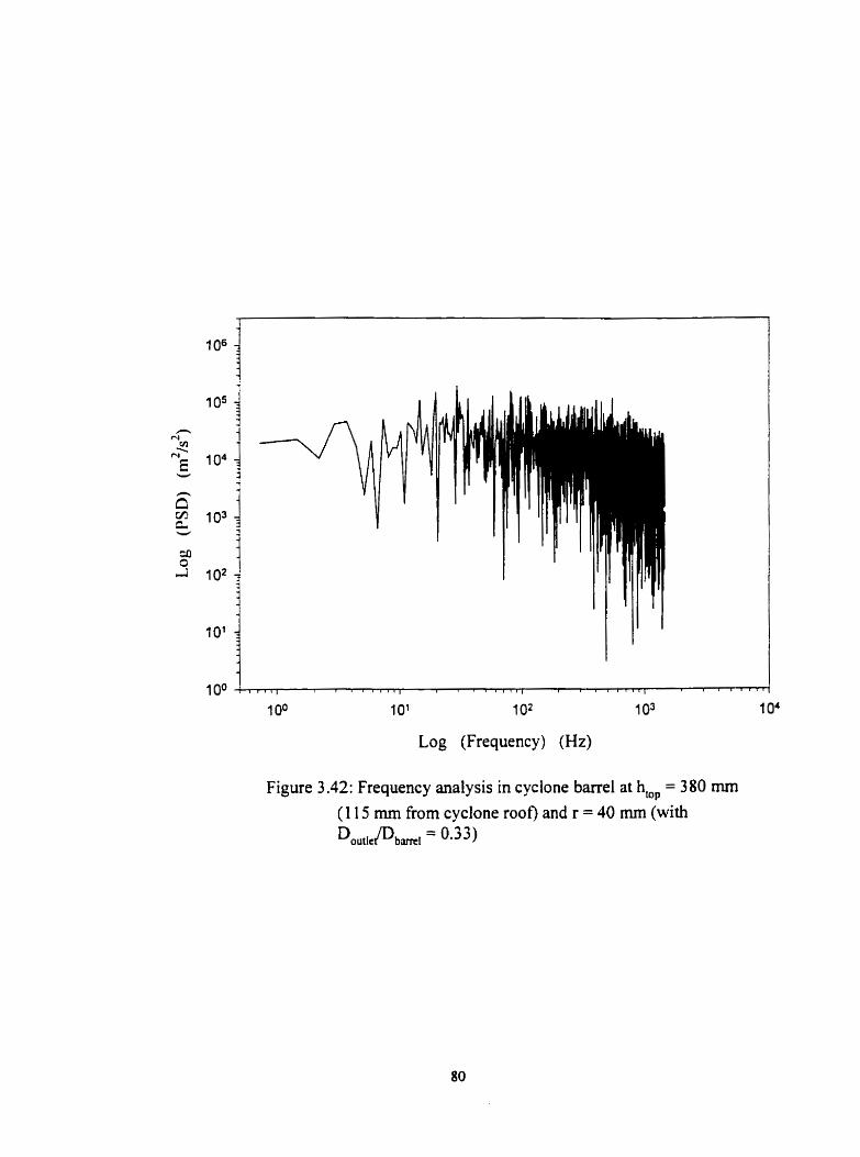
Log (Frequency) (Hz)
Figure 3.42: Frequency analysis in cyclone barre1 at h,,, = 380 mm
(1 1 5 mm from cyclone roof) and r = 40 mm (with D o " , , e P b m , =

1 o1 1 02 I 03
Log (Frequency) (Hz) Figure 3 .43 Frequency analysis in cyclone cone at hlop = 770 mm
and r = 25 mm (with Duutic(D,,, = 0.50)
0.00 0.02 0.04 0.06 0.08 0.10 Time Lag (s)
Figure 3.44: Autocorrelation coefficient in cyclone cone at hmp = 770 mm and r = 25 mm (with Douiic(D,,, = 0.50)

Tirne (s)
Figure 3.45: Time series of axial velocity in cyclone outlet at hm,, = 50 mm and r = 20 mm, at 50% motor load (with DOutkt/Db,, = 0.50)
1 O' 1 02 i o3 Log (Frequency) (Hz)
Figure 3.46: Frequency analysis in cyclone outlet at JO, = 50 mm and
r = 20 mm, at 50% motor load (with Do ,,,, ID ,,,, = 0.50)
0.00 0.02 0.04 0.06 0.08 0.10 0.12
Time Lag (s)
Figure 3.47: Autocorrelation coefficient in cyclone outlet at hm, = 50 mm and r = 20 mm, at 50% rnotor load (with D0,JDb,, = 0.50)
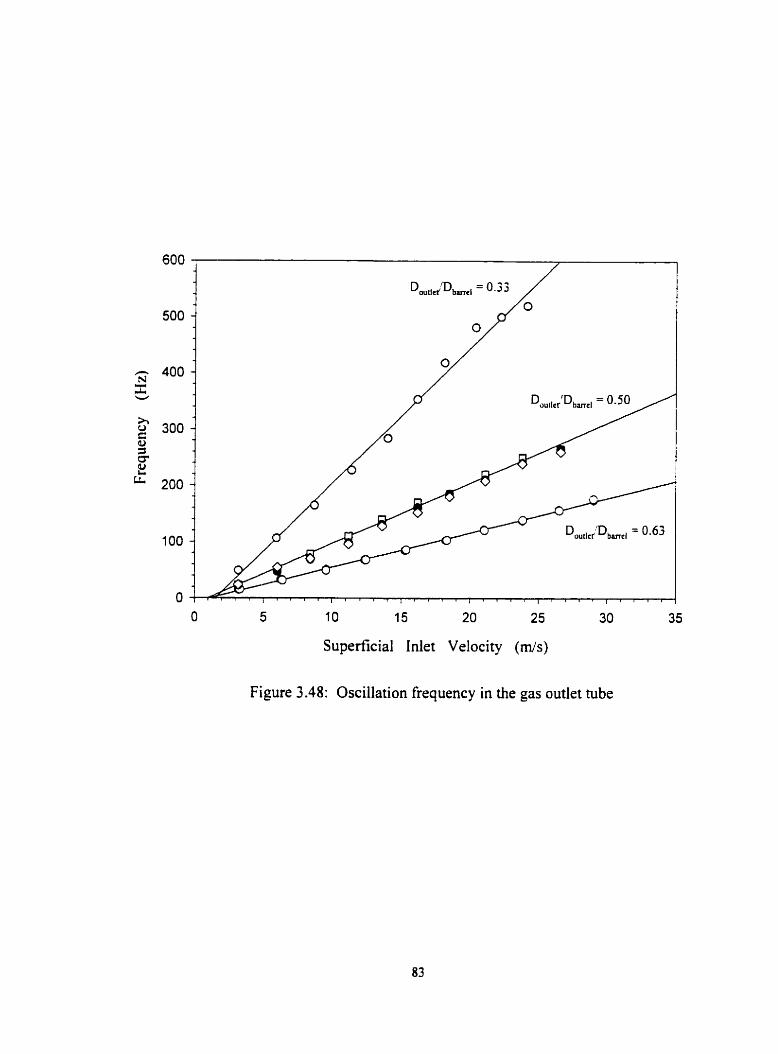
O 5 10 15 20 25 30 35
Superficial Inlet Velocity (mis)
Figure 3.48: Oscillation fiequency in the gas outlet tube
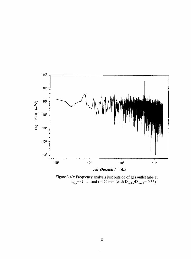
Log (Frequency) (Hz)
Figure 3.49: Frequency analysis just outside of gas outlet tube at hm,= - I mm and r = 20 mm (with Doutlr(Dbml = 0.33)

Radial Distance (mm)
Figure 3.50: Axial velocity profile 2 mm above the top of cyclone gas outlet tube (with D D,,, = 0.33)
-30 -20 -1 0 O 10 20 30 Radial Distance (mm)
Figure 3.5 1 : Axial rms velocity profile 2 mm above the top of cyclone outlet tube (with D ,,,,, JD,,, = 0.33)

Log ( Frequency ) (Hz)
Figure 3.52: Frequency analysis in cyclone outlet at hIop= 160 mm and r = 35 mm (with Doutiet/Dbur+, = 0.63)
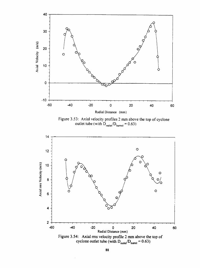
-6 O -4 0 -20 O 20 40 60
Radial Distance (mm)
Figure 3.53: Axial velocity profiles 2 mm above the top of cyclone outlet tube (with DoutiejD ,am, = 0.63)
-60 -40 -20 O 20 40 60 Radial Distance (mm)
Figure 3.54: Axial mis velocity profile 2 mm above the top of cyclone outiet tube (with D,,,JD,,, = 0.63)

References :
Benjamin, T. B., 1962, Theos. of the vortex breakdownphenornenon, J . Fluid Mech., 14,
593-629.
Boysan, F., B.C.R. Ewan, J. Swithenbank, and W.H. Ayers, 1983. Erperimental and
theoretical studies of cyclone separator uerodynamics. I.Chem. E. S ymp. Ser., 69. 3 05-
319.
Clark, R. L., W.F. Ng, D. A. Walker. and J. A. Schetz, 1990. Large-scale srructirre in a
supersonic dot-injectedjlowfieId. AIAA Journal. 28, 1045- 105 1
Grabowski, W. J., and S. A. Berger, 1976, Solurions of rhr Xavier-Slokes equafions for
vortex breakdown, J , Fluid Mech., 75,525-544
Faler. J.H., and S. Leibovich, 1977. Disrzrpted srates of vortexfTow and vortex
breakdown. The Physics o f fluids, 9. 1385-1400
Hall. M.G.. 1 966. The srructiire of concentrarecl vortex cores. Progress in Aeronautical
Sciences. 7,53-110
Hinze. J. 0.. 1975. Turbulence7 znd edition, Mc Graw Hill . Toronto.
Hussain Fazle A.K.M. 1 986, Coherent strzrctures and turbulence. J. FIuid Mech. 173
303-356.
Leibovich. S., 1984. Vortex stability and breakdown: survey and extension, AIAA
Journal, 22, 1 192- 1206.
Mees, A. J . Philip, 1990, Spectrum analysis of randornly sampled signals, a review,
Interna1 report. University o f Alberta, Edmonton.
Mees, P.A.J., 1997, Three dimensional transient gas cyclone simulations, 47" Canadian
Chernical Engineering Conference, Oct. 5-8, Edmonton, Alberta. Paper 482.
Press, W.H., B.P. Flannery, S. A Teukolsky, and W. T. Vetterling, 1989. Nmerical
Recipes, the art of scientifc computing, Cambridge University Press, New York.

Reynolds, A. J . , 1975, Turbulentflows in engineering. John Wiley & Sons
Squire, H. B. 1960, Analysis of the vortex breakdown phenornena. Parti , Aero. Dept..
Imp. Coli. Rep. No.102
Wills, J. A. B. 199 1 . Data sampling and data recovery, Experiments in Fluids. 12.23-28
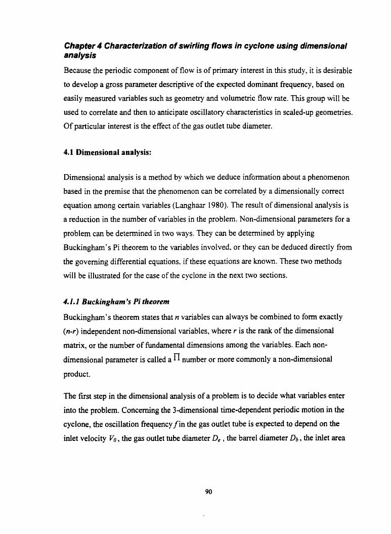
Chapter 4 Characterilafion of swirling flows in cyclone using dimensional analysis
Because the periodic component of flow is of primary interest in this study, it is desirable
to develop a gross parameter descriptive of the expected dominant fiequency, based on
easily measured variables such as geometry and volumetric flow rate. This group will be
used to correlate and then to anticipate oscillatory characteristics in scaled-up geornetries.
Of particular interest is the efTect of the gas outlet tube diameter.
4.1 Dimensional analysis:
Dimensional anaiysis is a method by which we deduce inf~rrnation about a phenomenon
based in the premise that the phenomenon can be conelated by a dimensionally correct
equation among certain variables (Langhaar 1980). The result of dimensional analysis is
a reduction in the number of variables in the problem. Non-dimensional parameters for a
problem can be determined in two ways. They c m be determined by applying
Buckingham's Pi theorem to the variables involved. or they c m be deduced directly from
the goveniing differential equations. if these equations are known. These two methods
will be illustrated for the case of the cyclone in the next two sections.
4.1.1 Buckingham 's Pi theorem
Buckingham's theorem States that n variables can always be combined to form exactly
(n-r) independent non-dimensional variables, where r is the rank of the dimensional
matrix, or the number of fundamental dimensions arnong the variables. Each non-
dimensional parameter is called a n number or more commonly a non-dimensional
product.
The first step in the dimensional analysis of a problem is to decide what variables enter
into the problem. Conceming the 3-dimensional tirne-dependent periodic motion in the
cyclone, the oscillation fiequency f in the gas outlet tube is expected to depend on the
inlet velocity Vo , the gas outlet tube diameter De , the barre1 diameter Db , the inlet area

Ain , the fluid density p, and fluid viscosity p. The functional dependence can be written
as:
in which the rank of the determinant is r=3.
To obtain ail the fundamental dimensions M (mass). L (length), and T (time). we can
choose a characteristic velocity, a characteristic length, and a fluid property as the
repeating variables in many fluid flow problems. In our case, Vo, D, and pare chosen.
Each non-dimensional product is formed by combining the three repeating variables with
one of the remaining variable. The results are as follows:
n, = v," ~ : ~ ' , 4 , , , = A,, / D,?
Therefore, the nondimensionai representation of the problem has the form:
The dimensionless products c m also be obtained by combining the four above. For
example, n, can be a fûnction of n, and the formation of n, / n, and retain either n2
n or 4, that is:
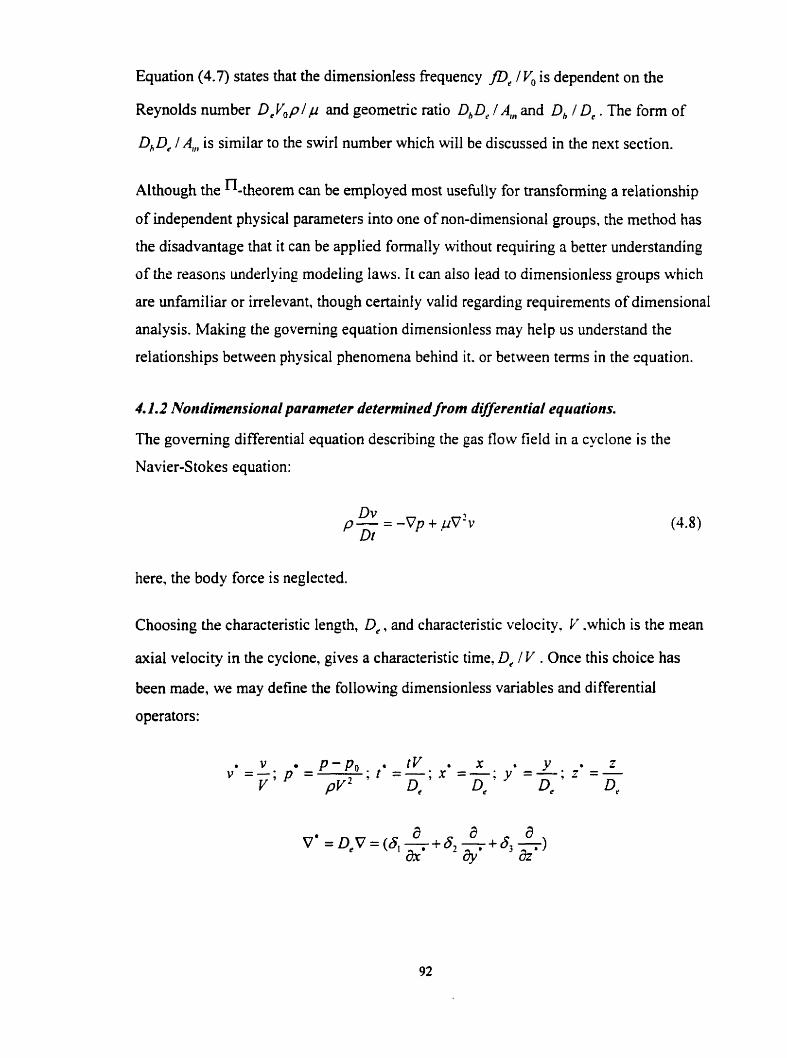
Equation (4.7) states that the dimensioniess fiequency fD, / V, is dependent on the
Reynolds nurnber D,V,p/p and geometrïc ratio D,D, / A,n and D, ID,. The fonn of
D,D, /A,,, is sirnilar to the swirl number which will be discussed in the next section.
Although the %heorern can be ernployed most usefully for trançforming a relationship
of independent physical parameters into one of non-dimensional groups. the method has
the disadvantage that it can be applied formally without requiring a better understanding
of the reasons underlying modeling laws. I r can aIso lead to dirnensionless groups which
are dami l i a r or irrelevant, though certainly valid regarding requirements of dimensional
analysis. Making the goveming equation dirnensionless rnay help us understand the
relationships between physical phenornena behind it. or between terms in the cquation.
4.1.2 Nondimensional parameter determin rd front dvferential equations.
The goveming differential equation describing the gas flow field in a cyclone is the
Navier-S tokes equation:
here, the body force is neglected.
Choosing the characteristic length, De. and characteristic velocity, I: .which is the mean
axial velocity in the cyclone, gives a characteristic time, De I V . Once this choice has
been made, we may define the following dimensionless variables and differential
operators:
. v p - p , a tV . x a y a z v =-; p =- ; t =- ; x =- , -. -- v p ~ " D e De De De
; Y =-• -
VI 2 1 a' az a2 = D;V- = - +-+- &' 2 'y? &' - '
by sening v = V'V , p - p, = p ' p ~ 2 , etc
t Since f = - (neglecting physical meaning. it bas the same units as frequency),
4 IC
Q = - D~'c~. substituting them into equation (4.9). and omitting **S. we obtain 4
0, Vp in which Re = - .
The Strouhal number is defined as - ' in this study , although the original form of the 0
Strouhal number is fD' . The Strouhal nurnber is a dimensionless group often used in v
time-dependent motion. Equation 4.10 indicates that the Strouhal number - is at least v a function of Reynolds number. Experiments have shown that the dimensionless
frequency is a function of both swirl number and Reynolds number (Griffiths et al. 1998).
For strongly turbulent flows, it is often assumed that turbulent difision dominates the
1 structure in such a way that the terms in equation (4.10) involving - can be neglected.
Re
This suggests that at high Re number, the Strouhal number should be independent of the
Reynolds number.
4.2 Swiri number
The most commonly used parameter for the characterization of swirling flows is the swirl
nurnber S,,,, which is a non-dimensional group representing the axial flux of swirl
momentum divided by the axial flux of axial momentum times the equivalent n o d e
radius (Gupta er al. 1984). In a physicai sense, the swirl number represents how much
axial mornentum the swirl needs to maintain advancing and rotating motion.
Experimental studirs show that the degree of swirl imparted to the flow has a large-scale
effect on the flow field. For example, in combustion, increasing the swirl cm cause jet
growth. entrainment. and progressively enhanced decay. The combustion intensity
(reacting flows) is affected by the degree of swirl imparted to the fiow (Lilley. 1977).
Various forms of swirl nurnber have been suggested. For example, in a jet. the swirl
number S , is related approximately by
in which 9 denotes the swirl vane angle. This expression illustrates that the swirl vane
angle is the key factor in determining the swirl in a jet since it is this angle that decides
the ratio of tangential component to axial component of velocity. The purpose of
determining the swirl number is to quantifi the flow phenomena, since the low swirl
phenomena are quite different fiom high swirl phenomena. For example, strongly
swirling flows (approximately Sw > 0.6) possess suficient radial and axial pressure
gradients to cause a central tororidal recirculation zone, which is not observed at weaker
degrees of swirl. Cassidy and Falvey (1970) have also shown that a series of non-
dimensionalized parameters are usehl for characterizing the precessing vortex core in
swirling flow. One of them is a momenturn parameter RD, / a', which can aiso be
related to the swirl number.
From the definition of swirl number, the swirl expression in a cyclone can be derived by
the following procedure:
The axial flux of angular momentum G, into a volume V through the surface element
dA is: GQ = ( r x w ) ( p . dA) (4.13)
since pu d4 is the axial mass flux through the surface element and r x w is the angular
momentum per unit rnass. Here r and u correspond to the location of cti . The axial flux
of axial (linear) momentum is:
since u is the axial momentum per unit mas . Integrating over the area under
consideration. the swirl number can be expressed as:
Here R, is the exhaust radius which is the radius of the gas outlet tube in the cyclone.
The pararneters of axial flux of angular momentum. which is the numerator of equation
(4.14), are taken fiom the barrel of the cyclone. since this is the input angular momentum.
The gas outlet parameters of the cyclone are applied for the calculation of axial flux of
axial momenturn that is in the denominator of equation (4.14). since this is the exit
momentum.
The swirl number should, if possible, be calculated from measured values of velocity. As
this is frequently not possible owing to a lack of detailed experimentai results. the swirl
number may be estimated from the geometry of the cyclone. To simplify equation (4.14)
to this form. three assumptions are made:
1) Uniforrn axial velocity profiles are imposed in both the barrel and the gas outlet tube,
although this is a major simplification. The ba i s for this assumption is fiom analysis of
plug flow in a free jet.
2) The local swirl velocity can be adequately represented by the inlet velocity.
3) A11 the gas flow exits From the gas outlet tube.
Applying these three assumptions, equations (4.1 2) and (4.1 3 ). become:
in which -A,,, is the tangential inlet area. R b is the barre1 radius, luid Q is the volumetric
flow rate at the inlet. Substituting (4.15) and (4. !6) into equation (4.14), we obtain the
swirl nurnber :
The expression for swirl number in equation (4.17) is a little different from the literature
(Yazdabadi et a/. 1994). The difference is that they do not have the coefficient 2/3 in the
expression of the swirl number.
The other way to sirnpliQ the equation is to assume that angular momentum is conserved
throughout the cyclone, instead of assuming a constant global swirl velocity. Then in
equation (4.14). r x w c m be taken out of the integral. The final expression for swirl
number is:
S, =- Ar,,
Equation (4.18) is the sarne definition as used by Yazdabadi et al. (1 994). Cornparhg
(4.18) to the texm A,JD& in equation 4.7, we can conclude that A,/DbD, term describes
the swirl motion in cyclone. The expression (4.18) is employed for swirl number in the
remainder of this study.
4.2.1 Ceneration of swirl and calculation of swirl number
Swirling flows are generated by three principal methods:
(a) tangentid entry of the fluid Stream, or of a part of it, into a cylindrical duct:
(b) the use of guide vanes in axial tube flow:
( c ) rotation of mechanical devices which impart swirling motion to the fluid passing
through them. This includes rotating vanes or grids and rotating tubes.
The swirl generated in a cyclone belongs to (a). Swirling flows having similar swirl
generators c m be characterized by the non-dimensional swirl number which is device-
iiidependent. The study of the swirl number is to provide critena to compare the flow
phenomena in similar generators. As mentioned before, when lacking accurate
measurements of local velocity in a cross section in cyclone and velocity varying dong
the fiow over the integral, we have to make several assumptions. This can cause
significant errors. For example. for higher degree of swirl. the axial velocity distribution
deviates considerably from plug flow. and the major portion of the flow leaves the gas
outlet near the outer edge (as shown in the previous chapter). Therefore the theoretical
correlation (4.16) will provide too low an estimate of the linear momentum. The sarne
situation occurs for calculation of angular momentum. For exarnple. when calculating the
Gd from equation (4.1 S ) , the deviation can be 20% compared with the original form of
equation (4.12), where we use the velocity profile at the top of the cyclone to calculate of
the angular momenturn in equation (4.12). Table 4.1 descnbes these errors in three
different gas outlet tube diameters.
Although using the geometry of the cyclone to calculate the swirl number is just a rough
estirnate, it gives us the basic critena to compare swirling flow phenomena in similar
geometries.
4.3 Strouhal number
The Strouhd nurnber is applied in frequency scaling for periodic flow structures. It is
often used to charactenze the oscillating wake in a Kamian vortex Street downstream of a
circular cylinder. The passage of regular vortices causes the velocity measurements in the
wake to have a dominant periodicity. The frequency fis expressed as a nondimensional
parameter known as Strouhal nurnber, defined as:
S,, = f i i O-,
in which Li, is the upstream velocity. and d is the cylinder diameter. The Strouhal
number cannot be interpreted as physically as the Reynolds number which is a ratio of
forces, but Zierep ( 1 971) explains it as the ratio of the local acceleration to the convective
acceieration in a flow field.
Shih et al. ( 1992) measured the frequency of oscillations near a lamina bcundary layer at
the exit of a rectangular jet. By using the Iaminar boundary mornentum thickness as the
length scale in the Strouhal nurnber and jet exit velocity as the uniform velocity. Le.
S , = f0 1 U c , in which Bis the initial momentum thickness. they concluded that the jet's
preferred Strouhal number is approximately proportional to die square root of the
Reynolds number.
In our study. the form used for Strouhal nurnber is:
since al1 the flow quantities are known at the exit, and it is easy to compare these results
with the available references.
In our experiment, the inlet volumetric flow rate is obtained by the inlet velocity
distribution rneasurement. The axial velocity profile at the top of the gas outlet tube is
also measured. giving us a volumetnc flow rate at the exit as well. Since the inlet
volurnetnc flow rate is lower than that of the outlet due to the compressibility of gas, al1
the volurnetric fiow rate cdculations at different gas outlet tube diameters are based on
the fiow at the top of the gas outlet tube. The fiequency of the oscillation is obtained by
analyzing the time series record using a fast Fourier transformation afier binning the
original data fiom the measurement.
4.4 Results
ID' (Strouhal nurnber). Three dimensionless parameters 4 0 / xD,v (Reynolds number), - 0
irRfR' (çwirl number) are utilized to correlate the experirnental data on frequency. and -
From Fig. 4.1. a plot of Strouhal number versus average-velocity Reynolds number at
different swirl number shows that the dimensionless frequency of the flow increases
rapidly with the increasing swirl number or Reynolds number but tends to have the trend
to become constant at a particular value of Reynolds number except S,.= 4.26. This also
indicates that the fi-equency of the flow is indeed essentially independent of viscosity for
a very large Reynolds number which is consistent with the dimensional analysis in
section 4.2. The three Iines with swirl number 2.208. 2.626 and 3.043 are taken frorn
Yazdabadi 's geometry (1 994). They fa11 approximately in the range that agrees with our
data. The reference data also show that there could be a minimum critical Reynolds
number below which no periodic motion would occur at any swirl number (the three lines
in reference do not pass through the origin when they are extended).
In Fig. 4.2. al1 the data collapse ont0 one line when SJS,, venus Reynolds nurnber is
plotted. At high Reynolds numbers. the rneasurernents show more scattering. This could
be due to the uncertainties at high velocity measurement. The figure indicates that for
different geometries, the S,,./Sw ratio is approximately a constant at a given Reynolds
number, i.e. the non-dimensional frequency scales linearly with the swirl at a given
Reynolds nurnber. The ratio of S,& increases parabolicdly with the Reynolds number
tilI50000. Beyond that cntical Reynolds nurnber, it seems that the non-dimensional
fiequency is only dependent on the swirl number.

These figures provide us with the information needed to predict the oscillation frequency
for different geometries and Buid properties. For example, if we scale up the geometry
with the sarne inlet velocity. the swirl number will be the same as before, and the
Reynolds will be increased, this will lead to a frequency decrease according to the above
correlation. Hot air flow with the same geometry and sarne volurnetnc flow rate will
cause a decrease in the frequency of the periodic motion in the cyclone since the
combined effect on the viscosity and density will Iead to a Reynolds number decrease.
Table 4.1 Simplified calculation of both angular momentum and linear momentum errors for three different gas outlet diameters
Go Error Eq. 4.12 vs. Eq. 4.15
Gz Error Eq. 4.13 vs. Eq. 4.16
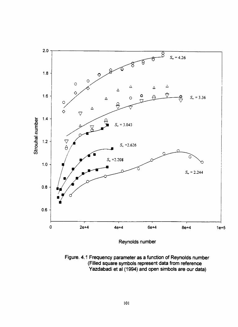
"i S,, =3.626
/
S,,. = 3 .Xi
Reynolds number
Figure. 4.1 Frequency parameter as a function of Reynolds nurnber (Filled square symbols represent data from reference Yazdabadi et al (1994) and open simbols are our data)

Sw=3.36 runl
S,,,=3.36 run2
Sw=3.36 run3
S,=4.26 runl
Sw=4.26 run2
Sw=2. 244
Sw=3. O43
Sw=2.626 Sw=2 .2O8
Reynolds number
Fig.4.2 Frequency swirl ratio as a function of Reynolds number. Open symbols are Our experimental data and filled symbols represent data from reference (Yazdabadi 1994)

Reference:
Cassidy, John J., and Henry T. Falvey, 1970,Obsen*ations ofunsteadyflow arising afier
vortex breakdown. J.Fluid Mech, 4 1.727-736
Griffiths, A.J., P.A. Yazdabadi, and N. Syred, 1998, Alrernative eddy shedding set up by
the nonaxisymrnetric recircdation zone a f the exhausr of a cyclone d m separator.
Journal o f Fluids Eng.. 120, 1 93- 199.
Gupta, A.K.. D. G. Lilley. N . Syred, 1984, Swirlflows. Abacus Press
Langhaar. L. H e m . 1980. Dimensional analysis and theory ofrnodels Huntigton . N.Y.
Lilley. David. G.. 1 977. Swirlflo ws in comblrstion: A review. AIAA Journal. 1 5. 1 063-
1 O78
S hih. C.. A. Krothapalli. and S. Gogineni. 1 992. Experimental observation of insrnbilip
modes in a rectangulur jet. AIAA Journal. 30. 1992.
Yazdabadi, P.A., A.J. Griffith. and N. S y red. 1 994. Investigations into the precessing
vortex core phenornenon in cyclone d m separators. Proc. 1. Mech. E.. 208, 1 47- 1 54.
Zierep, J., 197 1 . Sirnilarity lmvs and modeling. Marcel Dekker. Inc. New York
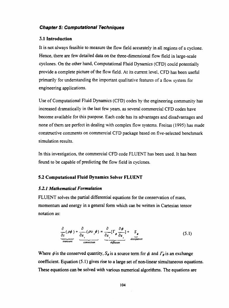
Chapter 5: Computational Techniques
3.1 Introduction
It is not always feasible to mesure the flow field accurately in all regions of a cyclone.
Hence, there are few detailed data on the three-dimensional flow field in large-scale
cyclones. On the other hand, Computational Fluid Dynamics (CFD) could potentially
provide a complete picture of the flow field. At its current level, CFD has been useful
primarily for understanding the important qualitative features of a flow system for
engineering applications.
Use of Computational Fluid Dynamics (CFD) codes by the engineering cornrnunity has
increased dramatically in the last few years. as several commercial CFD codes have
become available for this puopose. Each code has its advantages and disadvantages and
none of them are perfect in dealing with complex flow systems. Freitas (1 995) has made
constmctive cornrnents on commercial CFD package bbasd on five-selected benchmark
simulation results.
In this investigation, the commercial CFD code FLUENT has been used. It has been
fond to be capable of predicting the flow field in cyclones.
5.2 Computational Fluid Dynamics Solver FLUENT
5.2. I Mathematical Formulation
FLUENT solves the partial differential equations for the conservation of m a s ,
momentun and energy in a general form which can be written in Cartesian tensor
notation as:
Where 4 is the conserved quantity, S4 is a source terni for 4 and f4 is an exchange
coefficient. Equation (5.1) gives nse to a large set of non-Iinear simultaneous equations.
These equations c m be solved with various numerical algorithms. The equations are

reduced to their finite-difierence analogues by integrating over the computational cells
into which the domain is divided. After discretization. the resulting algebraic equations in
two dimensions for a general variable & can be written in the following common form:
Where
A,, = A , + A , + A , + A , - S ,
The nomenclature for these equations is displayed in Figure 4.1 which shows a typical
computational ce11 surrounding the node n, with neighboring nodes n, . n,, . n, and n, . The
coefficients &, -4 W. &, AS are the finite difference coefficients which combine
convection and diffusion through the control volume surrounding node n,. The quantities
Sp and Sc are components of the linearized source terms obtained in the finite difference
equation. Sd = SC + S P ~ , which incorporates any terms that do not fa11 into the
convectioddiffùsion form (5.1 ). n, is the central node relative to a computing ce11 and the
sumrnation is over the neighboring finite difference cells. Three different spatial
discretization schemes were used for the interpolation between g i d points and for the
calculation of the derivatives of flow variables: power-law, second-order upwind, and
QUICK, a bounded third-order method. These features are accessible through a
graphical-user interface permitting problem definition. problem solution, and post-
processing. The interested reader is referred to the user's guide for FLUENT (1 998). In
this investigation, discretization is done using a second-order finite difference upwind
scheme
Pressure/velocity coupling is achieved in the SIMPLE algorithm resulting in a set of
dgebraic equations which are solved by a line-by-line tridiagond multigrid method
and/or block-correction in terms of the primitive variables. The discretization and the
solution algorithm are well documented. A detailed discussion of the advantages and
disadvantages of the schemes rnay be found elsewhere, for example, Patankar (1 980).

5.2.2 Turbulence Models
Turbulent motion is extremely difficult to predict theoretically and experimentation is
expensive. In turbulent flows, the velocity at a point is considered as a sum of the mean
(tirne average) and fluctuating components:
The time-averaged mornentum equarion applied by FLUENT for turbulent flow is:
2 au, FLUENT ignores the term -p- under the assumption that the divergence of the
3 % velocity is negligible compared to the strain rate. The effect of turbulence is incorporated
- through the "Reynolds stresses" uttu; .
- Generally, turbulence models relate the turbulent Reynolds stresses u,h; to the average
au velocity gradient - by simple relationships as reviewed by White (1991) and Rodi
h,
(1980). The selection of a turbulence model for CFD prediction of flow fields is always a
concem. Of the more recent models, the K-E model. which was developed for isotropic,
fiee shear flows? has received wide acceptance in engineering applications. Details of the
transport equations with the standard K-E turbulence models in cylindrical coordinates
have been presented elsewhere (Ranade & Joshi, 1989). However, the turbulent flow
driven by the swirling motion in cyclone is not isotropic. FLUENT uses the standard K-E
turbulence model as default, but FLUENT aiso provides three options to select a non-
isotropic turbulence model for some applications. They are the Reynolds stress model
(RSM), the renormalized group K-E two-equation mode1 (RNG), and large eddy
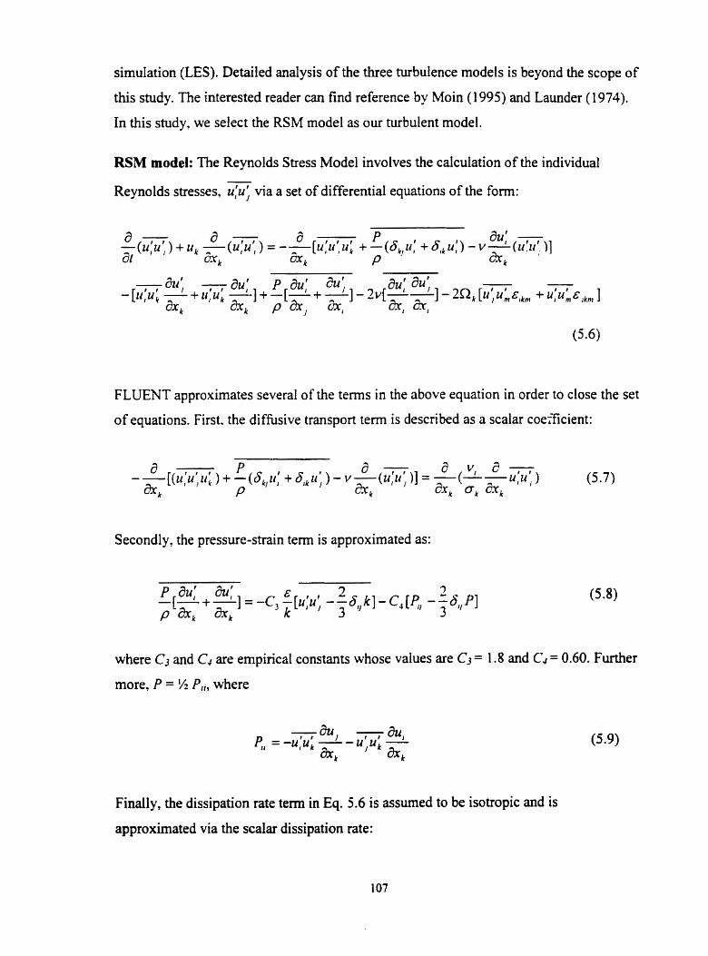
simulation (LES). Detailed analysis of the three turbulence models is beyond the scope of
this study. The interested reader c m find reference by Moin (1 995) and Launder (1974).
In this study, we select the RSM mode1 as our turbulent model.
RSM model: The Reynolds Stress Mode1 involves the calculation of the individual
Reynolds stresses, u,'u; via a set of differential equations of the form:
a - d - d - P du' - - ( u j / ) +., = ( 1 4 ) / , ) = --=-[u,'u)l; +-(QI: + & , , u : ) -v-(rr:uT )] di a, CrXk P &k
-"; - hl' P au: au; au; au; - - - [u:u; - + U I U k -1 + -[- + -1 - 2v[-- ùxk % P h, % 1 - 'Q, [ l 4 : ~ k ~ ~ k ~ + u : u I E ~ ~ ~ , 1 ax, hl
FLUENT approximates several of the ternis in the above equation in order to close the set
of equations. First. the diffusive transport term is described as a scalar coefficient:
Secondly, the pressure-strain term is approximated as:
where CJ and C4 are empirical constants whose values are C3 = 1.8 and CJ = 0.60. Further
more. P = !h P,,, where
Finally, the dissipation rate term in Eq. 5.6 is assumed to be isotropie and is
approximated via the scalar dissipation rate:
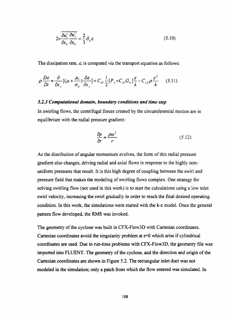
The dissipation rate. is computed via the transport equation as follows:
X2.3 Cornpuralional domuin, boundary conditions and tinte step
In swirling flows. the centrifugai forces created by the circumferential motion are in
equilibrium wi th the radial pressure gradient:
As the distribution of angular mornentum evolves. the f o m of this radial pressure
gradient also changes, dnving radial and axial flows in response to the highly non-
uniform pressures that result. It is this high degree of coupling between the swirl and
pressure field that makes the modeling of swirling flows cornplex. One strategy for
solving swirling flow (not used in this work) is to start the calculations using a low inlet
swirl velocity, increasing the swirl gradually in order to reach the final desired operating
condition. In this work, the simulations were started with the k-E model. Once the general
pattern flow developed, the RMS was invoked.
The geometry of the cyclone was built in CFX-Flow3D with Cartesian coordinates.
Cartesian coordinates avoid the singuiarity problem at r=O which arise if cylindrical
coordinates are used. Due to run-time problems with CFX-Flow3D, the geomets, file was
imported into FLUENT. The geometry of the cyclone, and the direction and ongin of the
Cartesian coordinates are show in Figure 5.2. The rectangular inlet duct was not
modeled in the simulation; only a patch from which the flow entered was simulated. In
simulation, the gas outlet barre1 ration is kept as 0.50, no different diameters have been
iried.
The grid size affected the accuracy as well as the efficiency of the numerical predictions.
Generally, a fine grid will yield better accuracy at the cost of additional computations. A
trade-off is ofien made to decide the optimum gnd size for a particular application. Many
authon have studied the effect of the grid size on the numerical predictions for the flow
field in swirling flows. The detailed grid size of the cyclone under study is given in Buns
(1996). In our study, we have tned three grid size. Since the grid is non-uniform, table
5.1 only provides a rough estimate of the grid size.
The boundary conditions at the inlet were measured values of mean velocities. turbulence
kinetic energy k and turbulence energy dissipation rate &. Remaining boundary conditions
were determined as given in the report by Buns (1 996). The boundary conditions are
surnrnarized as follows:
Velocity inlet boundary condition was imposed at the rectangular inlet patch with
only y component to be non-zero.
A 3% rnass flow condition was imposed at the underfiow (bonom of the cyclone).
An atmospheric pressure boundary condition was imposed at the overflow (top of the
cyclone) with specification of a static (gauge)pressure at the outlet boundary and al1
other quantities being extrapolated to the outlets from the interior.
The no slip condition was applied at the wall and on both surfaces of the gas outlet
tube.
FLUENT has the wall function built in as default. A detailed description of the wall
function is available (Launder & Spalding, 1974; Rodi, 1980). The wall function has
several advantages: (i) it requires less computer time and storage, (ii) it ailows the
introduction of additional empirical information, and (iii) it produces relatively
accurate results with fewer node points in the near-wall region. In essence. the wall
function relates the slip velocity near the wall U," to the wall shear through the
universal log law of the wall as:
where K, LI,, E and y are, Von Karmannos constant, the absolute value of the
velocity tangential to the wall, the roughness constant and the wall Reynolds number.
U'Y 1
' w 1 - respectively. The friction velocity u' is equd to (-1' . The denvation of the wall P P
function assumes an equilibrium between the generation and dissipation of turbulence
kinetic energy.
Since the simulation is time-dependent, the initial maximum time step was determined
using the Courant number. For a stable solution. the Courant number should be smaller
than 1.
The Courant number is the ratio of time step At to the characteristic convection time.
diLu, and is the time required for a disturbance to be convected a distance Ax. For c<l.
AtCAxlu. In our grid, Axlu is about 1 O". to get a converged solution at the beginning. lo4
was chosen as the initial time step.
FLUENT defines the residual as the imbalance in Eq. 5.2, summed over al1 the
cornputati~nal cells P. When the residuals are scaled. FLUENT scales the residual using a
scaling factor representative of the flow rate through the domain.
FLUENT defines the residual for pressure as the imbalance in the continuity equation:
where Cw, CE, CS, and CN are the convection of mass (kg/s) through each face of the
control volume surrounding node P. Scaled pressure residual is accomplished by dividing
by the residual at the largest absolute value of the continuity residual in the first five
iterations:
The scaled residual is a more appropriate indicator of convergence for most problems. In
our study, within each time step. the mass residual converged to less than 1 1 within
less than 20 iterations. The scaled residuals of converged to less than 1 1W5. as
recornrnended (Fluent Inc.. 1998). The solution process for the 3 dimensional. transient
CFD calculation is summûnzed in Figure 5.3.
5.2 Validation of CFD results
In computational fluid dynarnics. the validity of the numencal solution is usually
established by comparing the predicted flow field with well known cases of the
phenomenon under study. The quantity of numerical data acquired from the three-
dimensional simulation is extremely large. Experimental data are not as plentifùl as
numerical results. Therefore, the validation of the numerical CFD results is confined by
the available experimental data. The evaluation of the results of the numerical predictions
then becomes a reasonable task.
The validation of the CFD simulation has been performed with the following objectives:
Swirling motion in cyclone. This should include accurate results for the swirling
motion in both barre1 and the outlet. The swirling motion in the barre1 is shown in
Figure 5.4. In Figure 5.5, the swirl velocity exhibits the farniliar Rankine vortex
profile of a cyclone with the location of the two peaks of the simulation coincide with
the experiment peaks, but the agreement is qualitative only.
Two vortices in the flow field, Le. outer downward vortex and inner upward vortex.
Figure 5.6 shows the velocity vectors in a xz plane with large upward flow in the
middle and a small amount flow downward near the wail.

The qualitative agreement between the numencal CFD prediction and the expenmental
data is discussed in the next section.
5.3 Numerical results versus experimeotal results
Based on validation of the CFD numerical prediction for the basic flow pattern in
cyclone, a prediction of periodic motions in different elevations on monitoring points is
presented. The mean velocity and the fluctuation velocity in compatison with
experimental data are to be analyzed.
Before presenting the results, the quantities obtained in the numencal simulation have to
be clarified due to the presence of periodic motion. To analyze the flow field in the
context of more generai theones. let us consider the fluctuating velocity U 1 or velocity
disturbance. This is defined as:
where U,,, is the instantaneous velocity, and U, is the time-averaged (mean) velocity.
The instantaneous velocity is divided into two components in order to isolate the
turbulence from the mean flow field. Tropea et al. (1 989) suggest that a fùrther separation
is necessary for a flow field containing periodicity:
In this later representation, C I , is the randomly (true) fluctuating portion of velocity. U,
is the periodic portion of velocity at time t. The sum of U, + U , is the ensemble-
averaged mean velocity U, . In simulation, the time varying mean velocity is the
ensemble-averaged mean velocity . The axial fluctuating velocities are obtained by -
making square root of the Reynolds stress wt2 .
It is important to note that the solutions obtained fiorn the CFD simulations are unlikely
to be of any greater accuracy than results from, for example, the expenmental data.
Hence the CFD simulations, at the current level of development. are primarily a tool for
understanding the important features of a system and for predicting trends for scale-up
purposes.
5.4 Predictioa of the frequency of oscillation
The penodic motion observed in experiment was predicted by the numerical simulation.
Figure 5.7 is the mean axial velocity (no turbulent fiuctuating part) varying with time in
the gas outlet tube. The flow is marked with penodic motion oscillating at about 135 Hz
which is about half of the fiequency of the experimental at the same inlet velocity
(V,,=?6.677m/s and thef,,=260H=). Frequency analysis is no longer necessary since the
fiequency of the oscillation cm be calculated easily from the time varying plot when no
turbulent fluctuating velocity is showing there. By changing the inlet velocity. the
fiequency of oscillation changes as well. This c m be shown on the second and third part
of the oscillations in Figure 5.7. The frequency of oscillation scales with the inlet velocity
at the sarne slope as the experirnent (Figure 5.8).
The time varying mean velocities in barre1 and cone have also been plotted, they do not
show any stable oscillations (Figure 5.9 and 5.10). This is consistent with experimental
results. Contours of velocity or pressure at certain cross sections c m help us understand
the global fiow field in the cyclone. Figure 5.1 1 shows the contours of axial velocity in
which blue and red are downward and upward velocity respectively. At the very top
center part of the gas outlet tube, the axial velocity is negative which indicates the
existence of back flow. It is interesting to note that there is a helical wave in the cone.
This may reveal that the periodic motions at the top of gas outlet tube are attributed to
helical waves triggered by dynamic instability in the upstream flow at the cone. A rather
fascinating feature. not readily identifiable From Figure 5.1 1, but clearly visible in the
animation is that the helix emanates from the bottom of the cyclone, moving along a
circular trajectory, centered around the a i s . As clearly seen in the animation, the spiral
rotates in the same direction as the iniet flow.
5.4.1 Time averaged velocity prediciion
The time averaged velocity is obtained by integrating the time varying velocity over one
complete cycle. This is quite complicated, since the history information of veiocity
cannot be stored in the data file in FLUENT. instead, only the last interation information
is retained. The time varying velocities can only be stored at several monitoring points,
and FLUENT 5.0.2 only allows 1 1 monitoring points at maximum. Although FLUENT
c m autosave the data file at specific intervals during a calculation, this requires huge
amount of disc space. In our case, the tirne varying data are acquired through the
monitoring points. Figure 5.12 and Figure 5.13 show the time averaged axial velocity and
rms velocity profile at a z=0.738m (corresponding to the position of 9Omm from the top
of gas outlet in experirnent) in comparison with the experimental results. It indicates that
the simulation can follow the basic trend of the experimental data but under predicts both
the mean and the fluctuating velocity. The tirne averaged mean velocity and fluctuation
velocity profile are plotted at another elevation of 135mm from the top of gas outlet tube
(Figure 5.14 and Figure 5.1 5). In Figure 5.14. the time averaged mean velocity agree
quite will with the experiments, Le. the basic flow at this position has been predicted. but
the fluctuating velocity (Figure 5.15) is in extremely poor agreement with the measured
levels. This discrepancy is because in experirnent. both random turbulent fluctuation and
penodic motion contribute to the rms velocity. but in simulation, only turbulence
fluctuations are counted in the Reynolds stress.
From the above comparison, it c m be concluded that the application of the CFD
techniques has advanced to an extent that once a set of reliable boundary conditions has
been provided, the numericai visualization of the entire flow field can be achieved with
reasonable accuracy. On the otlier hand. the experimental measurements are quite
limited due to the experimental dificulty including seeding in the center. It should be
emphasized that the results of the numerical CFD simulations presented here give a
qualitative understanding of the overall flow characteristic rather than precise numerical
values themselves.

5.4.2 Solution sensitivity
A gird resolution study, performed by refining the number of grid points at the nearest
layer of boundary and at the near z axis region (as s h o w on Figure 5.16), which results
in 5 times the number of cells as the original one, did not significantly alter the results.
Al1 the cells in this calculation are in hexahedral shape. The diagonal appeared in the
cells in Figure 5.15 is due to the projection of the side of cells from the other layers. The
tirne step sensitivity and differencing scheme sensitivity have also been examined. The
time averaged mean velocity changes when using a different size of tirne step as shown
on Figure 5.17. Switching from the higher upwind (second order accurate) discretization
scheme to the quick (third order accurate) scheme does not change the solution.
5.5 Possible reasons for the discrepancy between experiment and simulation
The difference between the numerical results of the CFD simulations and the
experimental data c m be mainly attributed to approximations in the rnodeiing. the
boundary conditions. and possibly to uncertainty in the experimental data. We discuss
some of these below.
Wall fùnction approximation:
The application of a wall function is needed since not al1 turbulence models are valid in
the near wall region (y ' < 30). The wall fùnction approach works well when the
underlying assumption of an equilibrium turbulent boundary layer is satisfied. This
assumption breaks d o m when the boundary layer contains a significant pressure
gradient, a near stagnant or re-attachent point, or a region of high curvature. The
physical presence of swirling flow provides the highest curvature. It is suspect to assume
equilibrium between the turbulence energy production rate and turbulence energy
dissipation rate in such a flow. It may be better to investigate such a flow field by
avoiding the wall fùnction. FLUENT has extended the RSM model to the near wail
region but it requires more demanding computing resources. It is still not clear that the
extended RSM model will give more reasonable results, especially for the highly
swirling flow in cyclone.
O Uncertainty in static pressure:
In the CFD simulations with FLUENT, no static pressure information is needed as input
in the boundary condition for starting the calculations, as long as the flow field is not a
supersonic flow. FLUENT assumes that the static pressure in the flow field follows from
the pressure set up by the flow through the domain. However, in a flow with strong
swirling motion, it is the high degree of coupling between the swirling motion and the
pressure gradient that makes the CFD simulations so complex as shown in Eq. 5.12. The
uncertainty in static pressure may be a reason for some of the unreasonable results from
the current version of FLUENT.
O Uncertainty of the experimmtal data
Velocity bias is an error indigenous in the statistical analysis from the individual
realizations of the LDA measurements. The probability of measuring a velocity larger
than mean is greater than the probability of measuring a velocity slower than the mean.
The reason for this is that at high velocities. more fluid and more seeding particles pass
through the probe volume. per unit time. than at lower velocity. Thus the statistical mean
velocity is expected to be biased towards the high velocity (McLaughlin & Tiederman.
1973). This bias is believed to be systematic (Edwards. 1987). Several bias corrections
have been proposed and discussed. However. none is perfect. Edwards (1 987)
recornmends a residence time weighting correction. Since in our measurement. there is
no correction for mean velocity, and the gas flow is quite high. This kind of bias may
exist.
Uncertainty of the boundary conditions
At the top of the gas outlet tube, we impose a pressure boundary condition, i.e. the value
of static pressure is used. Al1 other flow quantities are extrapolated from the interior.
This boundary condition c m greatly attenuate the swirl in the cyclone. For this highly
swirling flow, the outlet pressure boundary condition may contnbute significantiy to the
improper prediction of numencal simulation.
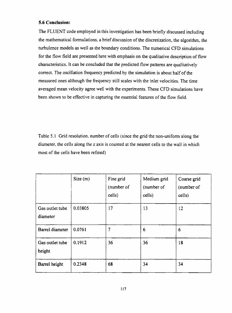
5.6 Conclusion:
The FLUENT code employed in this investigation has been briefly discussed including
the mathematical formulations, a brief discussion of the discretization, the algorithm. the
turbulence models as well as the boundary conditions. The numerical CFD simulations
for the flow field are presented here with emphasis on the qualitative description of fiow
characteristics. I t can be concluded that the predicted flow patterns are qualitatively
correct. The oscillation fiequency predicted by the simulation is about half of the
measured ones although the fiequency still scales with the inlet velocities. The time
averaged rnean velocity agree well with the experirnents. These CFD simulations have
been shown to be effective in capturing the essential features of the flow field.
Table 5.1 Grid resolution. number of cells (since the grid the non-uniform along the
diameter. the cells along the z axis is counted at the nearest cells to the wall in which
most of the cells have been refined)
1 Gas outlet tube
Barre1 diarneter
Gas outlet tube
height
Si te (m) Fine grid
(number of
cells)
Medium grid
(number of
cells)
Coarse grid
(number of
cells)
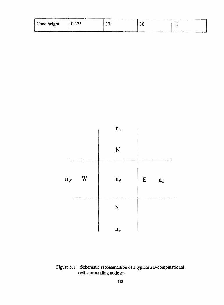
Figure 5.1 : Schematic representation of a typical 2D-computational ce11 surroundhg node n p
118
Cone height 0.3 75 30 30 15
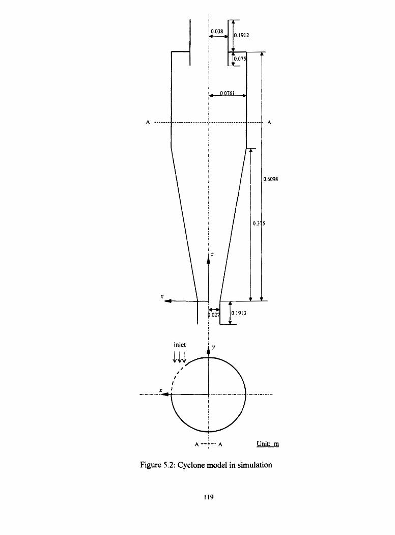
Unit: m
Figure 5.2: Cyclone mode1 in simulation
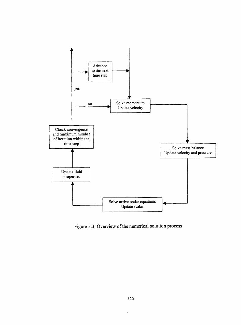
to the next time step
Check convergence and maximum number of iteration within the
time step
no b
Update fluid properties
Solve momentum Update velocity
Solve mass balance Update velocity and pressure
Figure 5.3: Overview of the numerical solution process
Solve active scalar equations Update scalar
+
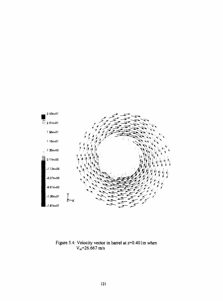
Figure 5.4: Velocity vector in barrel at ~ 0 . 4 0 1 rn when Vh=36.667 mis
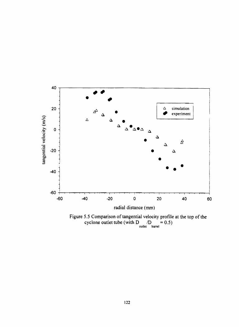
. & simulation
CI O experirnent
A 4 .
radial distance (mm)
Figure 5.5 Cornparison of tangential velocity profile at the top of the cyclone outlet tube (with D ID = 0.5)
outlet barre1
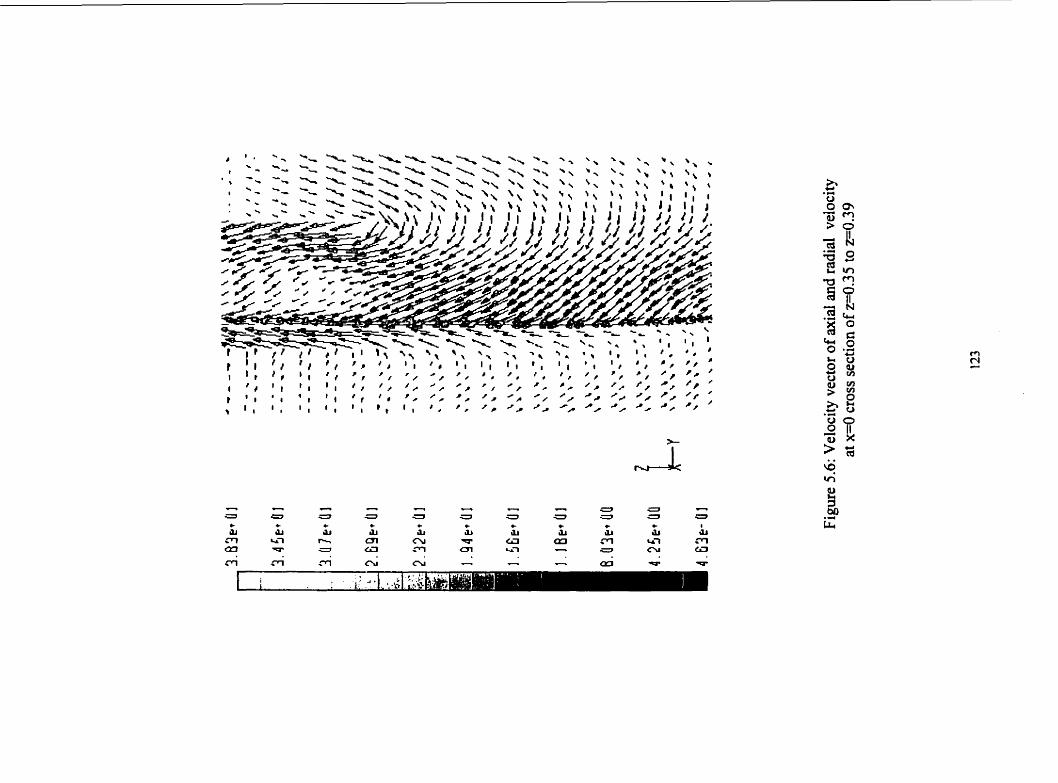
0 - c. - - - - CI r ) a C1
3 J 3 3 a 3 = a w + C + t t t C + * t I U ili SI rZI ili dJ ili ili ili il, il, .FI hl h al nl v O 43 .Pl u-7 .cl a3 V J cl -3-l Ol &AT - 3 C U 0
.cl .C1 ."1 Cu cw - - - m w v
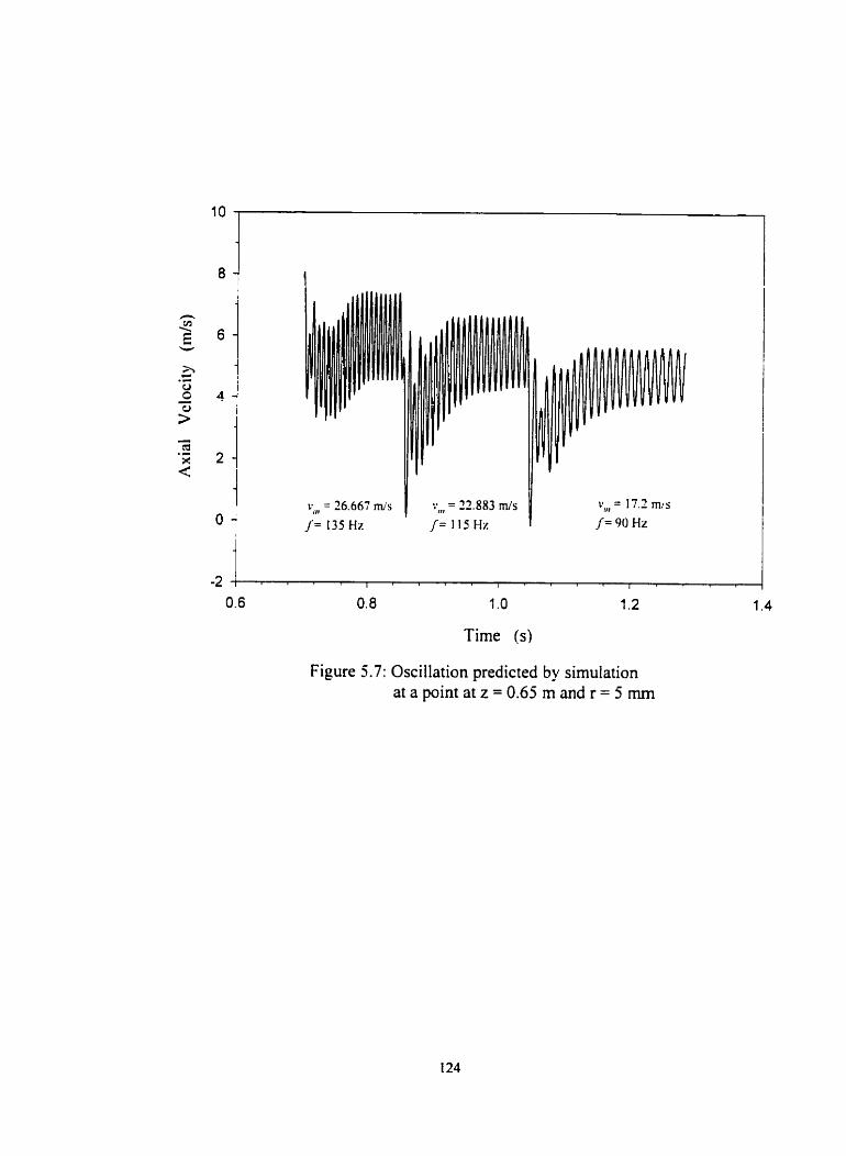
v,,, = 1 7.2 m's f = 90 Hz
0.6 O. 8 1 .O 1.2 1.4
Time (s)
Figure 5.7: Oscillation predicted by simulation at a point at z = 0.65 m and r = 5 mm

12 14 16 18 20 22 24 26 28
inlet superficial velocity mls
Figure 5.8. Frequency change with time in numerical simulation

0.6 0.7 0.8 0.9 1 .O 1.1 1.2 1.3 1.4
Time (s)
Figure 5.9: Oscillation darnping predicted by numerical simulation in cyclone barre1 at z = 0.5 m and r = O mm
0.6 O. 7 0.8 0.9 1 .O 1.1 1.2 1.3 1.4
Time (s)
Figure 5.10: Oscillation damping predicted by numencal simulation in cyclone cone at z = 0.3 m and r = 5 mm

Figure 5.1 I : Axial velociq contour on the xz plane.
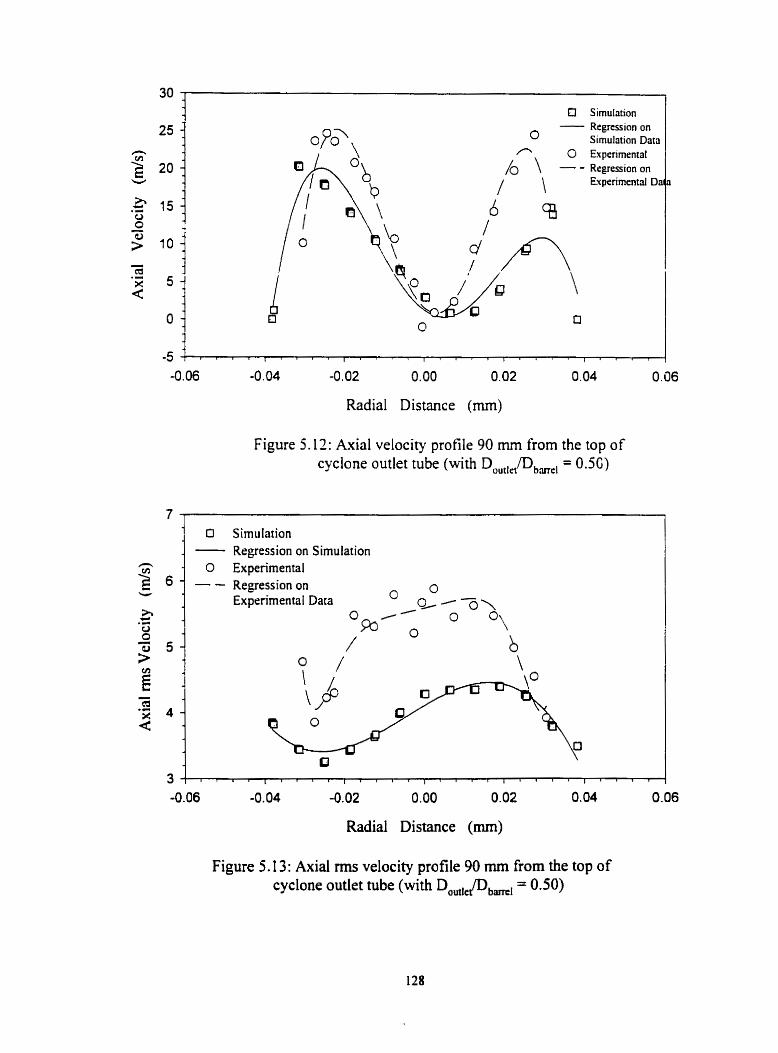
Regression on Simulation Data Experirnental Regression on Experimentai Da a
Radial Distance (mm)
Figure 5.12: Axial velocity profile 90 mm frorn the top of cyclone outlet tube (with D /D = 0.56)
] O Simularion
4 - Regression on Simulation Experimental Regression on Experimental Data
-0.06 -0.04 -0.02 0.00 0.02
Radial Distance (mm)
Figure 5.13: Axial rms velocity profile 90 mm fiom the top of cyclone outlet tube (with Dauller/Dbml = 0.50)
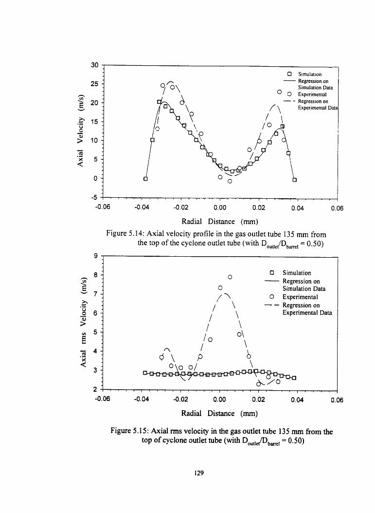
Radial Distance (mm)
Figure 5.14: Axial velocity profile in the sas ourlet tube 135 mm from the top of the cyclone outlet tube (with Doutic/D,,, = 0.50)
Radial Distance (mm)
9
Figure 5.15: Axial rms velocity in the gas outiet tube 135 mm fiom the top of cyclone outlet tube (with D ,,, Pb,, = 0.50)
8 - h
-È - 7 - P-t @ .- 8 6 1 - ::
O O Simulation - Regression on
O Simulation Data
/-' O Experimental \ -- Regression on
1 ' \ Experimental Data
1 \ I o O\ \
.I a P b 3 - \
2 1 . . , . . . . , . . . . , . . . . , . . . , . , , ,
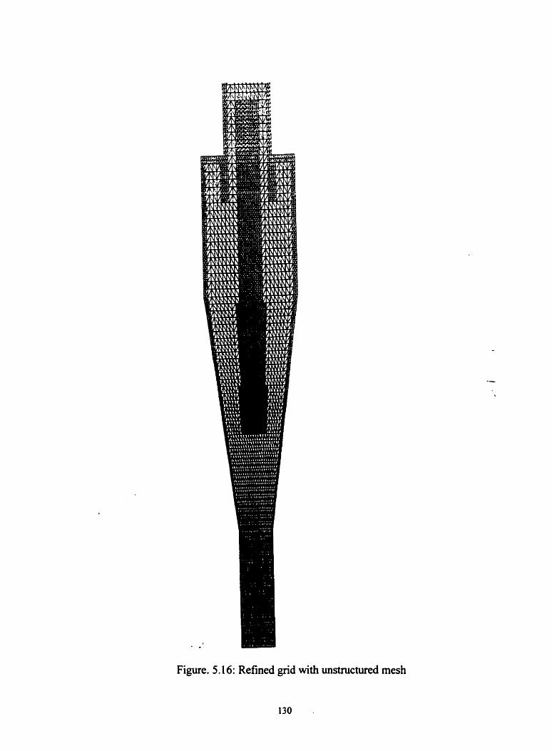
Figure. 5.16: Refined grid with unstructured mesh
130 .
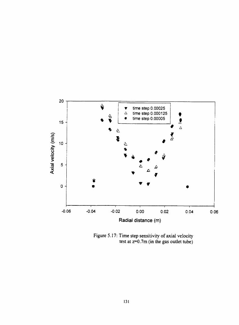
1
tirne step 0.00025
A
Radial distance (m)
Figure 5.17: Time step sensitivity of axial velocity test at z-0.7m (in the gas outlet tube)
Reference
Brodkey, R. 1995, Turbulence in Mixing Operations. Academic Press. New York
Butts, R., 1 996, Single phase CFD simulation of a cyclone separafor. Intemal report,
Department of Chernical & Materials Engineering, University of Alberta
Edwards, R. & A. Dybbs, 1984, Refrective index rnatching for velocity measurements in
complex geometries, TSI Quaterly 10 3.
Freitas, C. 1995, Perspective: Selected benchmarks fiom commercial CFD code. ASME
J. Fluid Eng.. 117.208.
Launder. B. & Spalding. D. 1974. The nirrnericaI cornplitution of turbtilentj7ows.
Comput. Methods Appl. Mech., 3.269.
McLaughlim. D. & W. Tiederman 1 973. Biasing correcfion for individual realizutionof
laser anemomrtry meastuement in turbulentfloivs. Physics o f Fluids. 16. 208
Patankar. S. & Spalding. D. 1980. A calc~rlation procedure for heat, mass and momentzm
tramfir in three-dimensional parabolicflo~vs, Int. J . Heat and Mass. Tram fer. 15, 1 787.
Ranada. V. & Joshi, J . 1989, Flow generated by apitched blade tiirbinr-II: Mathematical
mode1 and cornparison with experimenfal data, Chem. Eng. Cornm.. 81.225.
Rodi, W. 1980, Turbulence mode2 and their applicurion in hydrauiics. A state of the art
review, International Association for Hydraulic Research, Delft, The Netherlands.
Tropea, C.. M. Streglmeier, and W. Dursthoff 1989. The application of LDA to the
measurement of wave induced velocityfields. in IAHR workshop on instrumentation for
hydraulics laboratories, CC1 W, 16 August. Burlington, Canada
Chapter 6: Conclusions
A scaied down Stairmand cyclone was built in the lab to investigate the back fiow and the
oscillation in the gas outlet tube, especially when changing gas outlet diarneter and inlet
velocity. Large amplitude, highly penodic, non-axisymmetric fluctuations were observed
at the top of the gas outlet tube. Energy spectra constructed from instantaneous velocity
components in these regions display strong peaks. establishing the organized and penodic
nature of the flow. We may summarize Our findings as follows:
The oscillations and the back fiow decay progressively down the gas outlet tube. At
the top, periodic motions contribute significantly to the velocity fluctuations. while
down the gas outlet tube. they are almost negligibie.
The fiequency of the oscillations scaled with the inlet superficial veiocity for al1 the
three gas outlet tube diameter tested. Increase the gas outlet tube diameter will
decrease the frequency, and vice versa.
The non-dimensional frequency. Le. the Strouhal nurnber. was found to be a function
of both the swirl number and Reynolds nurnber. The constant ratio of Strouhal
number to the swirl number at a given Reynolds nurnber provides usehl information
to scale up geometry.
Applying Navier-Stokes equation explained that the strong swirling motion is the
cause of reverse flow and with a small diameter gas outlet tube cm attenuate the
distance back flow in the gas outlet tube.
The numerical CFD simulation using FLUENT cm predict flow pattern qualitatively
correct and effective in capturing the essentiai features of the swirling flow based on
our available experimental data. The frequency detected in simulation is about half of
the expenments.
The experiments do not allow conclusions to be drawn conceming the mechanisrn of
the oscillation. We are unable to detemine if the non-axisymmetric geometry is
related to the oscillations and back flow.