A NOVEL RATIOMETRIC METHOD FOR DETERMINING THE CONSEQUENCES OF

CELL-SIZED FEATURES IN A MICROFLUIDIC GENERATOR

OF CONCENTRATION GRADIENTS

By

Arunan Skandarajah

Thesis

Submitted to the Faculty of the

Graduate School of Vanderbilt University

in partial fulfillment of the requirements

for the degree of

MASTER OF SCIENCE

in

Biomedical Engineering

December, 2009

Nashville, Tennessee

Approved:

Professor John P. Wikswo

Professor Chris J. Janetopoulos

ii

ACKNOWLEDGEMENTS

I have to begin with the professors and advisors who made this research possible. I would

like to thank Professor John Wikswo for offering me the first hints of science’s true complexity

and for the practical components of securing funding, providing resources, and serving as a

reader of this work. I greatly appreciated the direction and focus Professor Christopher

Janetopoulos provided, the time he set aside to discuss all manner of scientific issues, and his

input in my writing process. I will always be indebted to Phil Samson for being willing to

transfer to me some of his considerable expertise, for his patience, and for assistance throughout

my project. I would like to offer my gratitude to Professor Robert Roselli for his assistance with

this work and throughout my graduate career at Vanderbilt. I would like to thank Professor

Shane Hutson for several thoughtful discussions, as well.

Over the course of my research, the guidance that Dr. Carrie Elzie and Ron Reiserer

provided has been invaluable, as have Dr. Kevin Seale’s questions on the nature of a scientist. I

appreciate Adit Dhummakupt’s help with the facilities, especially at odd times of the day. I

would like to thank Holley Lynch and Sarah Earl for assistance with confocal microscopy and

Professor Dmitry Koktysh at the Vanderbilt Institute of Nanoscale Science and Engineering for

spectrophotometry training. Other members of the Vanderbilt Institute for Integrative

Biosystems Research and Education (VIIBRE), including Don Berry and Allison Price, have

been incredible technical and editorial resources.

I cannot thank my friends enough for sticking with me through all the times I could not

be back by a reasonable hour. Last, but certainly not least, I would like to thank my family for

providing the strength, day-to-day encouragement, and inspiration that drove me to finish this

project.

iii

LIST OF TABLES

Table Page

1. Percent Difference Resulting from Relaxing Mesh and Time Step Conditions ....................................................................................... 17

iv

LIST OF FIGURES

Figure Page

1. Schematic of the microfluidic chemotaxis device analyzed ...................................... 8 2. Example of a FEM and time evolution of gradients ................................................ 12 3. Model of spatial variation of the gradient ................................................................ 19 4. Absorption spectra for Alexa Fluor 488 and 568 ..................................................... 21 5. Image correction for height effects in fluorescence intensity .................................. 22 6. Image correction for proximity and edge effects in fluorescence intensity ................................................................................................. 24 7. Comparison of modeled and ratiometrically corrected intensity data .................................................................................................................. 26 8. Axial intensity profiles in intensity generated by confocal microscopy ................................................................................. 28 9. Effects of cell occlusion on gradient formation ....................................................... 29 10. Effects of cell adhesion on gradient formation ........................................................ 31 11. Effects of loading density on gradient formation ..................................................... 33

v

TABLE OF CONTENTS

Page

ACKNOWLEDGEMENTS ................................................................................................ ii

LIST OF TABLES ............................................................................................................. iii

LIST OF FIGURES ............................................................................................................ iv

Chapter

I. INTRODUCTION ................................................................................................ 1

II. A NOVEL RATIOMETRIC METHOD FOR DETERMINING THE CONSEQUENCES OF CELL-SIZED FEATURES IN A MICROFLUIDIC

GENERATOR OF CONCENTRATION GRADIENTS .............................................. 3

Introduction .................................................................................................... 4 Materials and Methods ................................................................................... 7 Results .......................................................................................................... 16 Model Sensitivity to Meshing and Time Step Conditions .................. 16 Modeling of Gradient Stability and Homogeneity .............................. 17 Spectrophotometry .............................................................................. 20 Correction of Fluorescence across Regions of Varying Channel Height...................................................................... 20 Correction of Fluorescence Intensity in the Proximity of PDMS Microstructures .................................................. 23 Experimental Validation of Finite Element Model ............................. 25 Gradient Quantification along the Optical Axis .................................. 25 Modeling of Cell Occlusion and Cell Spreading Effects on Gradient Development ....................................................... 27 Modeling of Cell Loading Density on Gradient Formation ................ 28 Discussion .................................................................................................... 34 Representative Chemotaxis Device ..................................................... 34 Effects of Device Microstructure on Gradient Formation .................. 36 Consequences of High Fluorophore Concentration and the Use of Multiple Fluorophores................................................. 36 Quantification of Fluorescence Intensity through Ratiometric Image Correction ............................................................. 38 Potential of Ratiometric Methods for the Study of Partitioning Effects ......................................................................... 40 Ratiometric Correction for the Measurement of Gradients along the Optical Axis ........................................................ 40

vi

III. CONCLUSIONS AND FUTURE DIRECTIONS ...................................................... 41 REFERENCES .................................................................................................................. 44

CHAPTER I

INTRODUCTION

With the advent of rapid prototyping, microfluidic systems have come to represent a new

paradigm for the study of biology with single-cell resolution and incredibly high throughput [1-

3]. These systems have gained prominence in the field for several reasons: reduced reagent

consumption; precision of device manufacture; automation and rapid control of experimental

conditions; and compactness of the systems themselves. Many of the most recent and

inexpensive generations of microfluidic devices utilize soft lithography of

poly(dimethylsiloxane), or PDMS, a well-characterized, optically transparent, biologically inert

polymer well suited for the patterning of complex geometries. Much of the physics and practical

considerations of transitioning to culturing and assaying cells on this scale has been elucidated in

recent years [3-5]. With this knowledge and any one of a number of devices that provide tunable

chemical stimuli, researchers can probe the pathways of cell signaling that underlie complex

behaviors including morphogenesis, the immune response, and wound healing [6-8]. These

systems have also been generalized and characterized in detail, allowing for robust

spatiotemporal control of signaling molecule concentration [9, 10].

Beyond control of the single parameter of concentration, microfabricated structures can

also be constructed to constrain cells in three dimensions through fairly simple one- or two-layer

fabrication, better mimicking the complexity of the cells' native environments [11]. This is

important because as cells detect chemical cues, they also integrate mechanical signals into their

responses. Systems incorporating both stimuli can then help explain the variety of cellular

2

behaviors that have multiple inputs. For example, integrated responses have been shown to

govern stem cell fate and differential proliferation in tissue constructs [11, 12]. Even in studies

that focus on response to gradients of concentration, there is a growing emphasis on replicating

the cellular microenvironment to make results more representative and in vivo-like [13].

Geometric features that control the cellular microenvironment, however, must be

fabricated on the scale of the cells they influence. While producing these features is not at the

limit of current fabrication techniques, the features themselves can confound the results provided

by the increasingly complex assays that study cell motility in response to chemical signaling.

Current methods for numerical gradient analysis and optical gradient quantification make certain

assumptions that must be re-examined in the face of using sophisticated microfabricated tools. In

this work, we consider three particular factors using a modern chemotaxis system. First, we

demonstrate that the introduction of microstructures alters both chemical and mechanical cues,

making it difficult to tease apart what combination of the two triggers the cellular response.

Second, we evaluate a multi-dye method for ratiometric correction specific to individual fields of

view. This is presented as an improvement over standard flat-field correction in addressing field-

specific height variation and edge effects [14]. Finally, we expand upon excellent prior work that

considered the effects of cell geometry on gradient formation at this scale [15]. While this earlier

work analyzed artifacts introduced by a single cell under different flow regimes, we demonstrate

the variation in gradient formation as a function of cell loading density and cell height in a

diffusion dominated system. This work aims to provide tools and analysis to aid in the design of

systems that manipulate and probe the cellular microenvironment.

3

CHAPTER II

A NOVEL RATIOMETRIC METHOD FOR DETERMINING THE CONSEQUENCES OF CELL-SIZED FEATURES IN A MICROFLUIDIC GENERATOR

OF CONCENTRATION GRADIENTS

Arunan Skandarajah1,2

Christopher J. Janetopoulos2,3,4 John P. Wikswo1,2,5,6

Philip C. Samson2,5

1Department of Biomedical Engineering Vanderbilt University

Nashville, TN

2Vanderbilt Institute for Integrative Biosystems Research and Education Vanderbilt University

Nashville, TN

3Department of Biological Sciences Vanderbilt University

Nashville, TN

4Department of Cell and Developmental Biology Vanderbilt University

Nashville, TN

5Department of Physics and Astronomy Vanderbilt University

Nashville, TN

6Department of Molecular Physiology and Biophysics Vanderbilt University

Nashville, TN Corresponding Author: Philip Samson Physics and Astronomy Box 1807, Station B Vanderbilt University Nashville, TN 37235 615-343-4124 FAX: 615-322-4977 philip.samson@vanderbilt.edu

4

Introduction

The ability of cells to detect and migrate directionally in response to a gradient in

chemical stimuli is known as chemotaxis. This phenomenon underlies physiologically relevant

behaviors in humans such as morphogenesis, wound healing, the immune response, and

metastasis [7, 8, 16, 17]. In addition to its role in mammalian systems, chemotactic processes are

pervasive in other organisms, as well. Experiments conducted on model systems such as the

social amoeba Dictyostelium discoideum have helped elucidate the conserved mechanisms which

regulate chemotaxis [18, 19]. Established devices used to study chemotaxis, including the

Boyden, Zigmond, and Dunn chambers [20-22], continue to provide insight into cellular

behavior in these and other contexts. As researchers have sought a more comprehensive and

quantitative understanding of the chemotactic response, the tools to assay chemotaxis have

themselves become more varied and precise. A major advance predicated on microfluidic

technology was the active-flow gradient generator from Jeon et al., which was fabricated by

standard soft lithography and offered the ability to create complex gradients and either maintain

or rapidly switch them as necessary [6, 7, 23]. Systems based on the active mixing of a gradient

for application to cells have become widespread and have been characterized analytically by

several groups including our own [9, 10, 24]. While these recent works demonstrate the precision

with which gradients can be produced, modeled, and used to explain observed behavior, cells are

actually integrating far more than just an individual chemical signal to drive their motility. The

most recently designed chemotaxis assay chips have sought to address two particular

confounding factors: flow-induced shear stress and cell-substrate interactions.

Flow, whether applied by microfluidic systems or in vivo, has been demonstrated to alter

5

the migration of cells during their response to chemotactic stimuli. For example, experimental

and numerical analysis of the micromixer introduced by Jeon et al. demonstrated that increasing

shear stress reduced expected chemotaxis while introducing a migration component in the

downstream direction [25]. For the in vivo case of wound healing, the laminar stress in blood

vessels has been shown to enhance endothelial cell motility to the wound site [16]. More recent

microfluidic systems have corrected for this complicating factor by either reducing convection in

the region of the cells with high-resistance impediments or by eliminating flow entirely by

returning to a passively driven system with gradients produced by diffusion in the absence of

convection. Examples of high-resistance impediments include a hydrogel layer that effectively

shields an existing gradient from the pressure associated with loading [26] and the use of

multiple layer heights to make transport by diffusion dominant over that by convection [27].

Devices that are sealed during observation to eliminate flow, such as the one analyzed in this

work, can maintain pseudo-steady-state gradients during a pre-determined experimental period

but cannot dynamically vary the applied gradient [28].

Cell/substrate interactions are being actively elucidated by biologists seeking to

understand migration within the full complexity of the body [29] and by tissue engineers using

three-dimensional cues to guide cells in their devices [30]. The simplest chemotaxis assays

present cells with a physiologically unrealistic substrate that is uniform and two-dimensional [21,

22]. While still working in two-dimensional space, other assays have micropatterned single

layers that can control cell adhesion to explore cell to extra-cellular matrix effects on directional

migration [31]. To better mimic the full three-dimensionality of cellular environments, several

current systems are utilized to study migration in porous hydrogels [13, 32]. Further systems

have integrated these biological gels with three-dimensional structures such as “micropegs” to

6

demonstrate micromechanical interactions and the resulting relationships with cellular phenotype

and differentiation [12, 30].

Rapid progress in the design, modeling, and validation of these microfluidic systems

offers improved tools for the study of chemotaxis. In transitioning to tools on the microfluidic

scale, many differences with macroscale culturing and experimental environments have been

considered, such as the relative volume of cells to media, the induced shear stress, and the high

local concentrations of secreted molecules [4]. The physics of microfluidics within biological

microelectromechanical systems has also been considered in great detail [3], from the dominance

of diffusion over convection at these scales to pumping systems based on surface energy [33]. In

the context of newer chemotaxis assays, cell-size features predominate and the cells themselves

can occupy a significant portion of the volume. While the perturbation of flow by a single cell

and the resulting changes in gradient formation have been studied in convection-controlled

systems [15], the consequences of microstructure geometry on more complex diffusion-

dominated systems have yet to be systematically elucidated.

In this work, we address the question of how gradient formation is altered by both the

presence of complex microstructures and the cells themselves. We use a combination of novel

imaging and modeling processes to explore this question. We first apply standard epi-

fluorescence imaging and numerical modeling tools to characterize a new flow-free microfluidic

device that provides both three-dimensional mechanical cues and chemical stimuli. After

considering the limitations of these techniques, we utilize a novel ratiometric variation on epi-

fluorescence. Unlike current single-dye ratiometric intracellular calcium measurement methods

[34], we present a more flexible multi-dye solution. We then evaluate this multi-dye method in

conjunction with confocal microscopy, determining whether this gives us the ability to more

7

accurately quantify gradient development in the region of three-dimensional structures than does

traditional optical sectioning. We also detail the capability to stringently analyze edge effects that

other imaging systems in less complex environments can neglect [35]. These tools may allow

researchers to separate optical artifacts from the potential partitioning of the small molecules that

are often used in chemotaxis assays. We also discuss the vulnerabilities of this technique and

outline further experiments and variations on this ratiometric paradigm for integration with other

imaging modalities. Finally, we utilize our verified computational model to consider the

sensitivity of gradient formation in this device to cell loading density and aspect ratio. The

approach and techniques we utilize reveal valuable information about the limitations of our

particular system. This process will also be of use in the rational design of any device that guides

or probes cells with a chemical gradient when the features of the device are themselves on the

order of the size of the cells.

Materials and Methods

Device Design and Fabrication

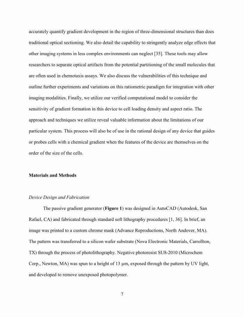
The passive gradient generator (Figure 1) was designed in AutoCAD (Autodesk, San

Rafael, CA) and fabricated through standard soft lithography procedures [1, 36]. In brief, an

image was printed to a custom chrome mask (Advance Reproductions, North Andover, MA).

The pattern was transferred to a silicon wafer substrate (Nova Electronic Materials, Carrollton,

TX) through the process of photolithography. Negative photoresist SU8-2010 (Microchem

Corp., Newton, MA) was spun to a height of 13 µm, exposed through the pattern by UV light,

and developed to remove unexposed photopolymer.

8

Figure 1: Schematic of the microfluidic chemotaxis device analyzed. A) An AutoCAD illustration of the entire device with the reservoirs for maximum and zero concentration indicated and sheath flow layers labeled with arrows; 25 µm circular posts used for support in the reservoir regions are omitted from the drawing for clarity. B) A close-up of the “ladder” of posts and clear regions along which the gradient forms. C) Posts and gaps are each 12 µm in the x and y dimensions.

12 µm

Central Loading Channel

12 µm

12 µm 100 µm

5 mm

12 µm

x

y

Chemoattractant Reservoir

Sink Reservoir

1

2

3

4

5

6

7

8

9

The process was repeated to overlay an additional 20 µm of SU8 to make the two sheath

flow layers connecting ports 2-6 and 4-8 (Figure 1A). A profilometer (Tencor Instruments

Alpha-Step 200 Profilometer, Milpitas, CA) confirmed the height of the SU8 mold within a

tolerance of less than 3 µm. To prevent adhesion of the cast poly(dimethylsiloxane) (PDMS)

device to the mold, the photoresist structure was silanized by chemical vapor deposition of

trimethylchlorosilane for at least 3 hours. PDMS (Sylgard 184, Dow Corning, Midland, MI) was

prepared in a 10:1 ratio of prepolymer to curing agent, poured onto the patterned master,

degassed for 20 minutes, and baked at 65 °C for at least 4 hours. Devices were separated from

the silicon substrate by cutting through the PDMS on the edges of the device with a scalpel

blade. Access ports 1-8 in Figure 1A were punched with 15 gauge stainless steel. The increased

height of channels connecting ports 2 to 6 and 4 to 8 allowed for precise loading into the

chemoattractant reservoir as described below. The initial cast was sectioned into thin slices and

visualized to check for definition of microstructures.

To limit rapid evaporation-induced convection in the device while allowing for high

magnification imaging, it was necessary to maintain near 100% humidity on a coverglass

surface. To accomplish this, we utilized “chambered” coverglass which consists of a coverslip

base with four plastic walls and a lid (Lab-Tek, Rochester, NY). To prepare devices for use, the

PDMS device and the coverglass chamber were exposed to oxygen plasma (Harrick Plasma

Cleaner/Sterilizer-32G, Pleasantville, NY) and the device was irreversibly bonded to the inner

coverglass surface of the chamber. The first stage of device loading was completed at this time to

maintain the hydrophilicity of the oxidized channels. After the second stage of device loading,

evaporation was controlled by wetting the inside of the chamber and sealing all gaps with

silicone grease before observation.

10

Device Loading

Alexa Fluors 488 and 568 conjugated to 10 kDa Dextran were purchased from Molecular

Probes (Eugene, OR). In the first stage of device loading, an aqueous solution of 50 µM of the

reference fluorophore was pipetted onto each port and was drawn into the channels by the initial

hydrophilicity of the channels. The device was then maintained in a humidity controlled system

for at least 4 hours to allow complete filling of the device by excess fluorophore solution on the

ports.

In the second stage of device loading, the chemoattractant reservoir (Figure 1A) was

loaded with 50 µM of the reference fluorophore as well as 50 µM of the second, diffusing

fluorophore. The rest of the device was not altered at this stage, remaining loaded with only 50

µM of the reference fluorophore. Hence the reference fluorophore was maintained at a

concentration of 50 µM throughout the device while the diffusing fluorophore was loaded only

in the chemoattractant reservoir, from which it was allowed to diffuse. The loading process relied

on surface energy driven flow [28]. Briefly, access ports 3, 4, 5, 7 and 8 in Figure 1A were

conformally sealed with PDMS patches to prevent evaporation. A 2 µL drop containing both the

reference dye and the diffusing fluorophore was placed on port 1. A solution containing only the

reference dye was pipetted to a volume of 5 µL on port 2 and 12 µL on port 6. To continue the

loading process, droplet volumes at ports 1 and 2 were maintained, consuming up to 15 µL of

each reagent. Visualization of loading was done on a Zeiss Axiovert 25 (Carl Zeiss

MicroImaging, Thornwood, NY) with a QImaging Cooled RTV Camera (Surrey, BC, Canada).

After confirming the complete filling of the reservoir, the remaining ports were sealed with

PDMS patches, and the device was set aside in a 100% relative humidity environment to allow

diffusive gradient formation with minimal evaporation-induced convection.

11

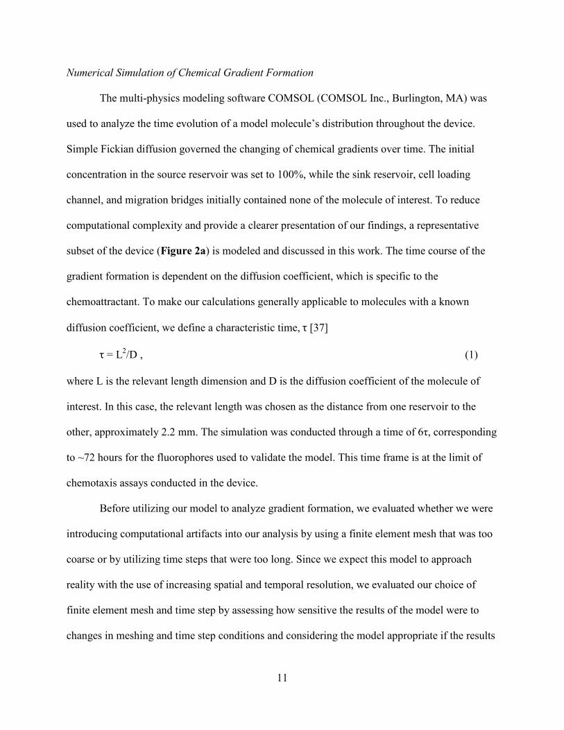
Numerical Simulation of Chemical Gradient Formation

The multi-physics modeling software COMSOL (COMSOL Inc., Burlington, MA) was

used to analyze the time evolution of a model molecule’s distribution throughout the device.

Simple Fickian diffusion governed the changing of chemical gradients over time. The initial

concentration in the source reservoir was set to 100%, while the sink reservoir, cell loading

channel, and migration bridges initially contained none of the molecule of interest. To reduce

computational complexity and provide a clearer presentation of our findings, a representative

subset of the device (Figure 2a) is modeled and discussed in this work. The time course of the

gradient formation is dependent on the diffusion coefficient, which is specific to the

chemoattractant. To make our calculations generally applicable to molecules with a known

diffusion coefficient, we define a characteristic time, τ [37]

τ = L2/D , (1)

where L is the relevant length dimension and D is the diffusion coefficient of the molecule of

interest. In this case, the relevant length was chosen as the distance from one reservoir to the

other, approximately 2.2 mm. The simulation was conducted through a time of 6τ, corresponding

to ~72 hours for the fluorophores used to validate the model. This time frame is at the limit of

chemotaxis assays conducted in the device.

Before utilizing our model to analyze gradient formation, we evaluated whether we were

introducing computational artifacts into our analysis by using a finite element mesh that was too

coarse or by utilizing time steps that were too long. Since we expect this model to approach

reality with the use of increasing spatial and temporal resolution, we evaluated our choice of

finite element mesh and time step by assessing how sensitive the results of the model were to

changes in meshing and time step conditions and considering the model appropriate if the results

12

Figure 2: A) Example of the result of a finite element model conducted in COMSOL. The rows in Table 1 correspond to the error between the coarse and fine variants of the finite element model at the corresponding points a, b, c, and d. B) The time evolution of the gradient along the ladder as well as the steady-state solution for infinitely wide reservoirs.

A)

B)

a) b) d) c)

Central Channel

13

were insensitive.

After completing this initial evaluation of the modeling process, we utilized COMSOL to

evaluate the effects of PDMS microstructures, cellular occlusion, and cell density on gradient

formation. Utilizing steady-state and time-dependent 2-D models, we demonstrate the relative

significance of the spatial variation of the gradient caused by PDMS posts against the temporal

variation over the 6τ period of interest. We then considered a pseudo-3-D model in which we

approximate cell occlusion by reducing the effective diffusion constant in proportion to the

volumetric occlusion. Since occlusion is a function of both cell height and channel height, this

provides useful insight into the variation in the gradients that cells encounter as a function of

channel aspect ratio. Finally, we used images of cells in the device to create a probabilistic cell-

loading algorithm. By varying the density of cells, we demonstrate the sensitivity of both the

mean and variance of the gradients in the device to cell density.

Visualization of Chemical Gradient Formation

The time evolution of the chemical gradient in the xy plane of the device was imaged in

epi-fluorescence mode. Standard protocols were followed for maximizing dynamic range while

minimizing photobleaching of the specimens [14]. Images were collected using an Axiovert

200M (Carl Zeiss MicroImaging, Thornwood, NY) equipped with a CoolSnap camera (Roper

Scientific GmbH, Germany) and mercury arc lamp. The Alexa Fluor 488 was imaged using the

standard FITC filter set and the Alexa Fluor 568 was imaged with a TRITC filter set.

To evaluate how the gradients depended upon the location of the imaged region within

the height of the channel, we collected images at different heights on a Zeiss LSM410 laser-

scanning confocal microscope. For this system, the Alexa Fluor 488 was excited by the 488 line

14

of an Ar/Kr laser and fluorescence was collected through a 515-540 band-pass filter. The Alexa

Fluor 568 was excited by the 568 line and fluorescence was collected through a 580 long-pass

filter. Images in both wide-field and confocal mode were collected using objectives optimized

for flatness of field and minimal color dispersion. Images were exported as 16-bit TIFF files for

further analysis.

Spectrophotometry

A Carry 5000 spectrophotometer (Varian, Palo Alto, CA) was utilized to collect the

absorbance spectra across the visual spectrum for each dye utilized. A standard 1 cm path length

was used to confirm the absorption spectra provided by Molecular Probes and to evaluate the

degree of potential interaction among multiple fluorophores.

Two-Dimensional Standard and Ratiometric Image Processing

Images were imported into MATLAB and corrected by the standard one-color flat-field

correction and by the proposed two-color ratiometric method as described below. The standard

flat-field process, detailed by Murphy, involves the capture of three images: the raw frame, dark

frame, and flat-field frame [14]. The raw frame consists of the unprocessed specimen image

while capture of the dark frame simply follows the same protocol without the use of any

excitation source. This allows for measurement of the offset signal in the CCD and provides an

indication of the thermal noise. The flat-field frame is an image of a featureless and uniformly

dyed region that is further smoothed by averaging several images. The flat-field frame provides

information on the variation in the sensitivity of CCD pixels and uneven illumination resulting

from the optics. The corrected image is obtained by carrying out the following calculation on a

15

pixel-by-pixel basis,

( ( , ) ( , ))

( , )( ( , ( , ))Raw x y Dark x y

corrected x y MFlat x y Dark x y

−=

− , (2)

where the mean value of the raw image, M, is utilized as a common scaling factor for all pixels.

We describe this process as a single-color, field-flattening correction.

As an alternative to this process, we propose a multi-dye ratiometric correction that

utilizes a background and a spatially dependent illumination correction specific to each field of

view. The goal of this process is to correct for aberrations in illumination introduced by the

particular structures in the field of view – either light-piping due to edges of PDMS features, or

differences in channel heights. This process of image correction requires at least two

fluorophores. The reference dye, present at a uniform concentration throughout the device,

serves as an internal control for differences in the light path, channel depth, and the collection of

out-of-plane fluorescence observed at the boundaries of structures and walls in microfluidic

systems [35, 38]. Raw frames are captured for each fluorophore using the appropriate excitation

sources and filter sets. The exposure time for each fluorophore was chosen to maximize the

dynamic range and to reduce noise in the image while minimizing photobleaching. It is essential

that corresponding raw frames for the multiple fluorophores be collected in the same field of

view and at the same focal plane. To correct for improper registration in x-y of different

channels, ImageJ (NIH, Bethesda, MD) was used to align images. Instead of subtracting a

standard dark-field frame, we find the minimum pixel value in the frame and conduct a uniform

subtraction. This step attempts to eliminate the baseline autofluorescence and light-piping that

we expect in a field of view containing PDMS surrounded by a lower refractive index solution. If

an appropriate offset is not used for each field of view, the calculated intensity would no longer

be linearly related to fluorophore concentration when taking a ratio of the two frames. Finally,

16

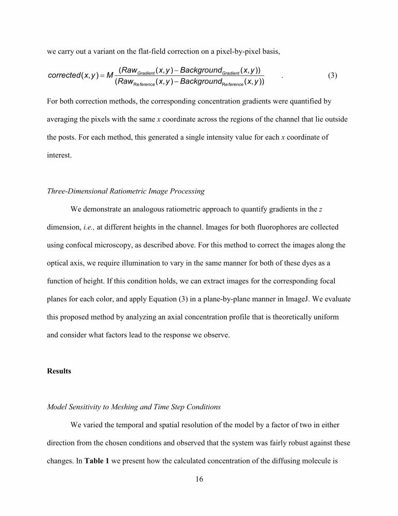
we carry out a variant on the flat-field correction on a pixel-by-pixel basis,

Re Re

( ( , ) ( , ))( , )

( ( , ) ( , ))Gradient Gradient

ference ference

Raw x y Background x ycorrected x y M

Raw x y Background x y−

=−

. (3)

For both correction methods, the corresponding concentration gradients were quantified by

averaging the pixels with the same x coordinate across the regions of the channel that lie outside

the posts. For each method, this generated a single intensity value for each x coordinate of

interest.

Three-Dimensional Ratiometric Image Processing

We demonstrate an analogous ratiometric approach to quantify gradients in the z

dimension, i.e., at different heights in the channel. Images for both fluorophores are collected

using confocal microscopy, as described above. For this method to correct the images along the

optical axis, we require illumination to vary in the same manner for both of these dyes as a

function of height. If this condition holds, we can extract images for the corresponding focal

planes for each color, and apply Equation (3) in a plane-by-plane manner in ImageJ. We evaluate

this proposed method by analyzing an axial concentration profile that is theoretically uniform

and consider what factors lead to the response we observe.

Results

Model Sensitivity to Meshing and Time Step Conditions

We varied the temporal and spatial resolution of the model by a factor of two in either

direction from the chosen conditions and observed that the system was fairly robust against these

changes. In Table 1 we present how the calculated concentration of the diffusing molecule is

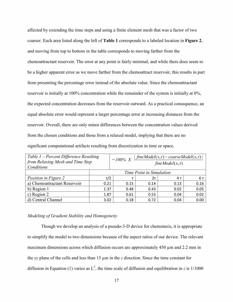
17

affected by extending the time steps and using a finite element mesh that was a factor of two

coarser. Each area listed along the left of Table 1 corresponds to a labeled location in Figure 2,

and moving from top to bottom in the table corresponds to moving farther from the

chemoattractant reservoir. The error at any point is fairly minimal, and while there does seem to

be a higher apparent error as we move farther from the chemoattract reservoir, this results in part

from presenting the percentage error instead of the absolute value. Since the chemoattractant

reservoir is initially at 100% concentration while the remainder of the system is initially at 0%,

the expected concentration decreases from the reservoir outward. As a practical consequence, an

equal absolute error would represent a larger percentage error at increasing distances from the

reservoir. Overall, there are only minor differences between the concentration values derived

from the chosen conditions and those from a relaxed model, implying that there are no

significant computational artifacts resulting from discretization in time or space.

Table 1 – Percent Difference Resulting from Relaxing Mesh and Time Step Conditions

=100% X ),(

|),(),(|txfineModel

txlcoarseModetxfineModel −

Time Point in Simulation Position in Figure 2 τ/2 τ 2τ 4 τ 6 τ a) Chemoattractant Reservoir 0.21 0.15 0.14 0.13 0.16 b) Region 1 1.37 0.48 0.43 0.02 0.05 c) Region 2 1.87 0.61 0.53 0.04 0.02 d) Central Channel 3.02 0.18 0.72 0.04 0.00

Modeling of Gradient Stability and Homogeneity

Though we develop an analysis of a pseudo-3-D device for chemotaxis, it is appropriate

to simplify the model to two dimensions because of the aspect ratios of our device. The relevant

maximum dimensions across which diffusion occurs are approximately 450 µm and 2.2 mm in

the xy plane of the cells and less than 15 µm in the z direction. Since the time constant for

diffusion in Equation (1) varies as L2, the time scale of diffusion and equilibration in z is 1/1000

18

of that in the other two dimensions. This means that, regardless of the molecule, any variation

across the height of the device would disappear almost instantly relative to the time it takes for a

gradient to form between the two reservoirs.

Since the chemoattractant reservoir depletes over time, we first used our model to

confirm that a sufficient gradient exists over the course of a proposed experiment. We

approximated the behavior of an average protein by utilizing in our COMSOL model the known

characteristics of 10 kDa dextran conjugated to a fluorophore. To generalize the results across

other fluorophores, data are described in normalized time and distance across the bridge (Figure

2). To determine whether the time variation in the gradient would be a significant contributor to

cell behavior, we also modeled the spatial variation resulting from device geometry (Figure 3).

By focusing on a 200 µm length of the bridge spanning regions with and without posts, it

becomes clear in Figure 3A that the concentration profile is not linear and is instead a function

of local device geometry. This difference can be more readily quantified by plotting the gradient

itself (Figure 3B) and comparing our design against an equivalent bridge with no posts. Over the

time frame of interest, these two figures demonstrate that the gradient encountered by a

theoretical cell is more strongly a function of spatial variation than of time.

The variation in the gradient along the length of a bridge can be replicated by replacing

complex regions obstructed by posts with simple regions with diffusivity values proportional to

the area that is unobstructed. This approximation can be made because spatial mass transfer is

the product of flux and the cross-sectional area; a change in one will have the same effect on the

product as a proportionally large change in the other. In concrete terms, a region that has 40% of

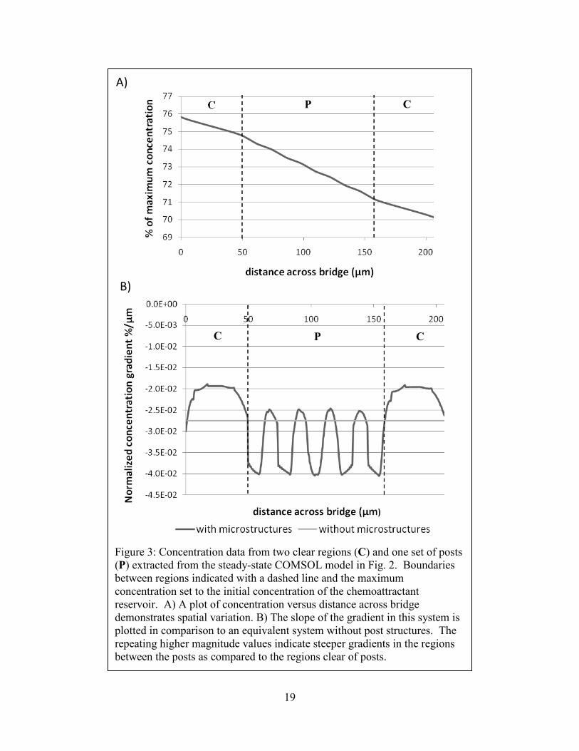
19

Figure 3: Concentration data from two clear regions (C) and one set of posts (P) extracted from the steady-state COMSOL model in Fig. 2. Boundaries between regions indicated with a dashed line and the maximum concentration set to the initial concentration of the chemoattractant reservoir. A) A plot of concentration versus distance across bridge demonstrates spatial variation. B) The slope of the gradient in this system is plotted in comparison to an equivalent system without post structures. The repeating higher magnitude values indicate steeper gradients in the regions between the posts as compared to the regions clear of posts.

A)

B)

P C

C P C

20

its area occluded by posts would result in the same gradient as a region without occlusion and a

diffusivity value of 60% of the unobstructed region. We extend this logic, which was described

for obstruction in the xy plane by the posts, in a later section to model cell occlusion in the z

dimension.

Spectrophotometry

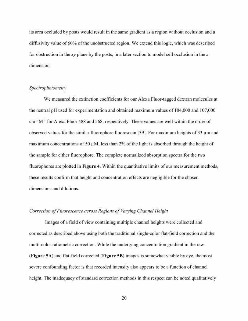
We measured the extinction coefficients for our Alexa Fluor-tagged dextran molecules at

the neutral pH used for experimentation and obtained maximum values of 104,000 and 107,000

cm-1 M-1 for Alexa Fluor 488 and 568, respectively. These values are well within the order of

observed values for the similar fluorophore fluorescein [39]. For maximum heights of 33 µm and

maximum concentrations of 50 µM, less than 2% of the light is absorbed through the height of

the sample for either fluorophore. The complete normalized absorption spectra for the two

fluorophores are plotted in Figure 4. Within the quantitative limits of our measurement methods,

these results confirm that height and concentration effects are negligible for the chosen

dimensions and dilutions.

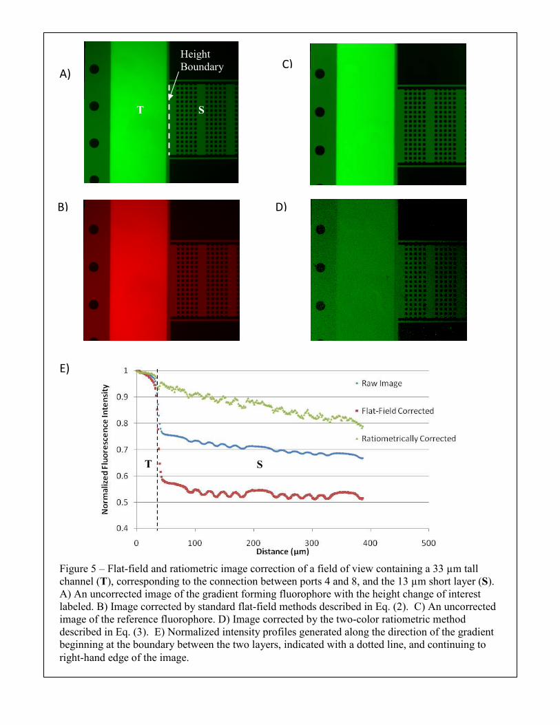
Correction of Fluorescence across Regions of Varying Channel Height

Images of a field of view containing multiple channel heights were collected and

corrected as described above using both the traditional single-color flat-field correction and the

multi-color ratiometric correction. While the underlying concentration gradient in the raw

(Figure 5A) and flat-field corrected (Figure 5B) images is somewhat visible by eye, the most

severe confounding factor is that recorded intensity also appears to be a function of channel

height. The inadequacy of standard correction methods in this respect can be noted qualitatively

21

Figure 4 – Absorption spectra for the dextran conjugated AlexaFluors utilized in fluorescence experiments normalized to the maximum absorbance value for each.

22

Figure 5 – Flat-field and ratiometric image correction of a field of view containing a 33 µm tall channel (T), corresponding to the connection between ports 4 and 8, and the 13 µm short layer (S). A) An uncorrected image of the gradient forming fluorophore with the height change of interest labeled. B) Image corrected by standard flat-field methods described in Eq. (2). C) An uncorrected image of the reference fluorophore. D) Image corrected by the two-color ratiometric method described in Eq. (3). E) Normalized intensity profiles generated along the direction of the gradient beginning at the boundary between the two layers, indicated with a dotted line, and continuing to right-hand edge of the image.

A)

B)

C)

D)

E)

Height Boundary

T S

T S

23

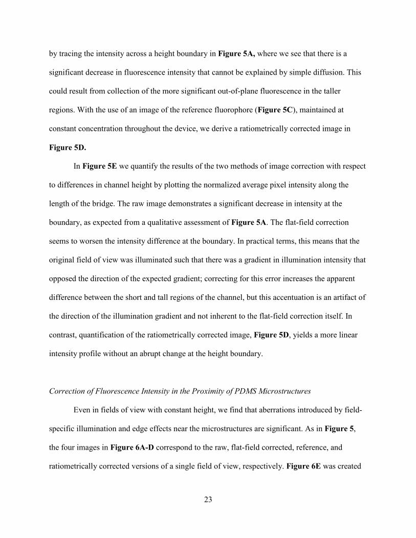
by tracing the intensity across a height boundary in Figure 5A, where we see that there is a

significant decrease in fluorescence intensity that cannot be explained by simple diffusion. This

could result from collection of the more significant out-of-plane fluorescence in the taller

regions. With the use of an image of the reference fluorophore (Figure 5C), maintained at

constant concentration throughout the device, we derive a ratiometrically corrected image in

Figure 5D.

In Figure 5E we quantify the results of the two methods of image correction with respect

to differences in channel height by plotting the normalized average pixel intensity along the

length of the bridge. The raw image demonstrates a significant decrease in intensity at the

boundary, as expected from a qualitative assessment of Figure 5A. The flat-field correction

seems to worsen the intensity difference at the boundary. In practical terms, this means that the

original field of view was illuminated such that there was a gradient in illumination intensity that

opposed the direction of the expected gradient; correcting for this error increases the apparent

difference between the short and tall regions of the channel, but this accentuation is an artifact of

the direction of the illumination gradient and not inherent to the flat-field correction itself. In

contrast, quantification of the ratiometrically corrected image, Figure 5D, yields a more linear

intensity profile without an abrupt change at the height boundary.

Correction of Fluorescence Intensity in the Proximity of PDMS Microstructures

Even in fields of view with constant height, we find that aberrations introduced by field-

specific illumination and edge effects near the microstructures are significant. As in Figure 5,

the four images in Figure 6A-D correspond to the raw, flat-field corrected, reference, and

ratiometrically corrected versions of a single field of view, respectively. Figure 6E was created

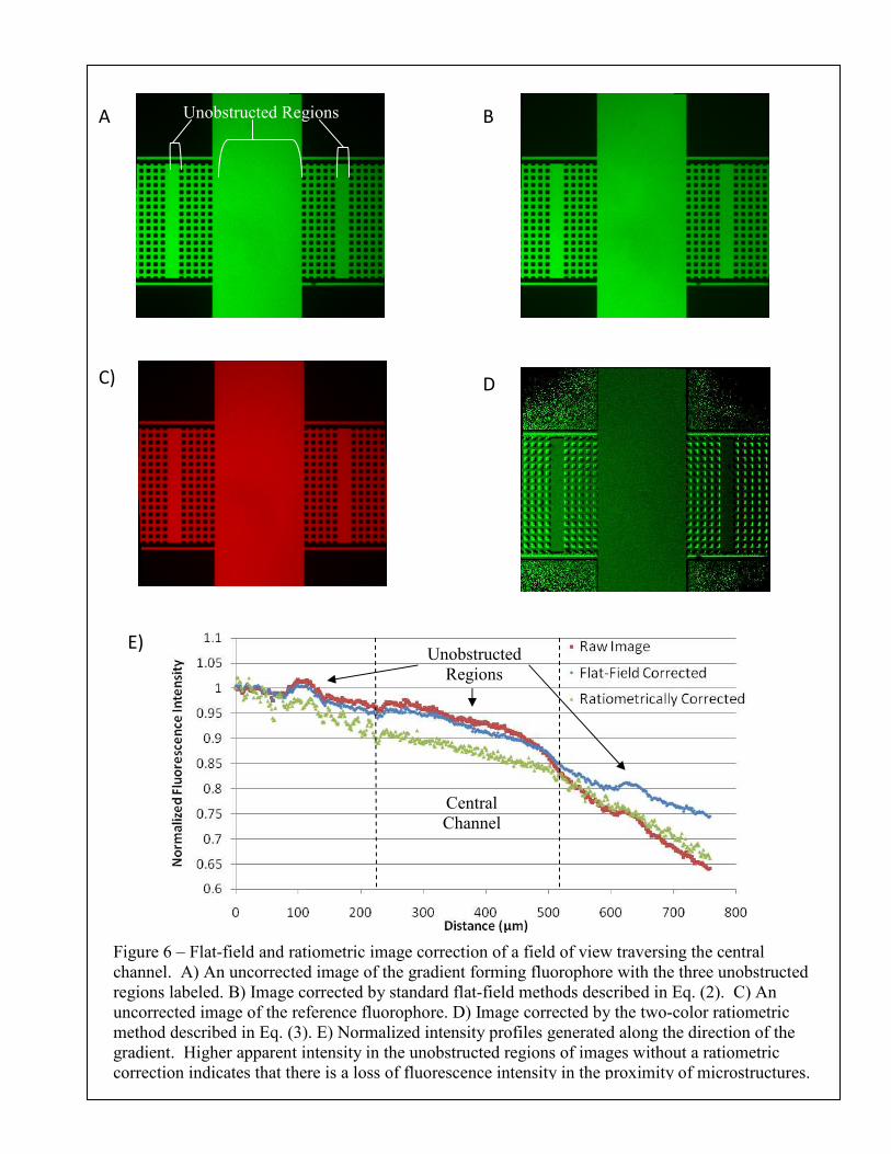
24

Figure 6 – Flat-field and ratiometric image correction of a field of view traversing the central channel. A) An uncorrected image of the gradient forming fluorophore with the three unobstructed regions labeled. B) Image corrected by standard flat-field methods described in Eq. (2). C) An uncorrected image of the reference fluorophore. D) Image corrected by the two-color ratiometric method described in Eq. (3). E) Normalized intensity profiles generated along the direction of the gradient. Higher apparent intensity in the unobstructed regions of images without a ratiometric correction indicates that there is a loss of fluorescence intensity in the proximity of microstructures.

A)

B)

D)

C)

E)

Central Channel

Unobstructed Regions

Unobstructed Regions

25

by calculating the average pixel intensity along the length of the bridge, excluding the pixels that

correspond to the posts. The non-ratiometrically corrected images in this set demonstrate a loss

of fluorescence intensity in the proximity of the posts. This shadowing effect results in higher

overall intensities in the three unobstructed regions of the field of view that are illustrated in

Figure 6A. Figure 6E demonstrates that the flat-field correction, which uses a featureless

correction image, does not affect the shadowing in the proximity of the microstructures. The use

of the ratiometric correction, however, does lead to an intensity profile without higher apparent

intensity regions in unobstructed regions.

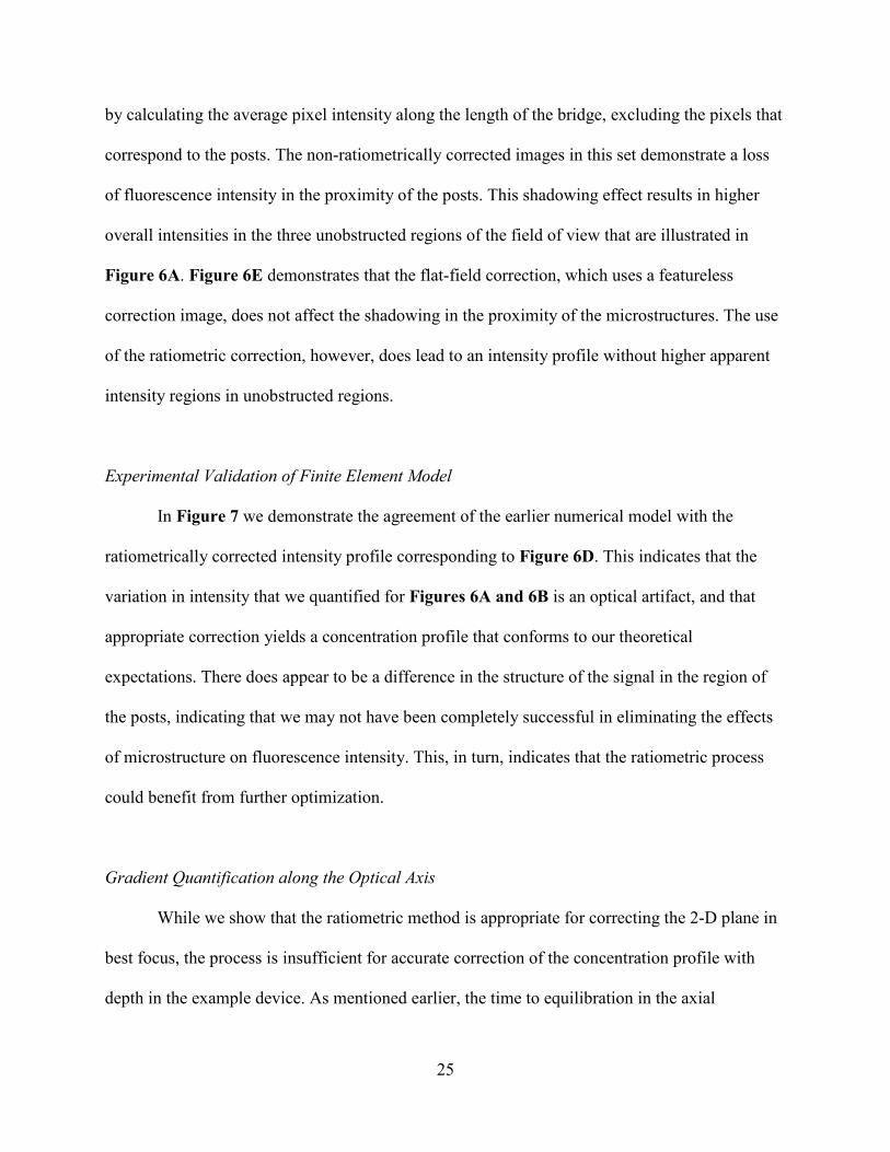
Experimental Validation of Finite Element Model

In Figure 7 we demonstrate the agreement of the earlier numerical model with the

ratiometrically corrected intensity profile corresponding to Figure 6D. This indicates that the

variation in intensity that we quantified for Figures 6A and 6B is an optical artifact, and that

appropriate correction yields a concentration profile that conforms to our theoretical

expectations. There does appear to be a difference in the structure of the signal in the region of

the posts, indicating that we may not have been completely successful in eliminating the effects

of microstructure on fluorescence intensity. This, in turn, indicates that the ratiometric process

could benefit from further optimization.

Gradient Quantification along the Optical Axis

While we show that the ratiometric method is appropriate for correcting the 2-D plane in

best focus, the process is insufficient for accurate correction of the concentration profile with

depth in the example device. As mentioned earlier, the time to equilibration in the axial

26

Figure 7 – The ratiometrically corrected data from Figure 6 and the corresponding model data are plotted as a function of distance along the bridge, normalized to the same maximum concentration.

27

dimension is much faster than equilibration of the gradient between reservoirs, so we expect a

uniform axial concentration for this device’s aspect ratio over the time frames of these trials. A

first step to the correction process is determining whether the axial intensity profiles of the two

fluorophores are similar enough that applying a ratiometric correction will correct the variation

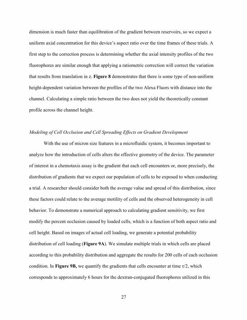
that results from translation in z. Figure 8 demonstrates that there is some type of non-uniform

height-dependent variation between the profiles of the two Alexa Fluors with distance into the

channel. Calculating a simple ratio between the two does not yield the theoretically constant

profile across the channel height.

Modeling of Cell Occlusion and Cell Spreading Effects on Gradient Development

With the use of micron size features in a microfluidic system, it becomes important to

analyze how the introduction of cells alters the effective geometry of the device. The parameter

of interest in a chemotaxis assay is the gradient that each cell encounters or, more precisely, the

distribution of gradients that we expect our population of cells to be exposed to when conducting

a trial. A researcher should consider both the average value and spread of this distribution, since

these factors could relate to the average motility of cells and the observed heterogeneity in cell

behavior. To demonstrate a numerical approach to calculating gradient sensitivity, we first

modify the percent occlusion caused by loaded cells, which is a function of both aspect ratio and

cell height. Based on images of actual cell loading, we generate a potential probability

distribution of cell loading (Figure 9A). We simulate multiple trials in which cells are placed

according to this probability distribution and aggregate the results for 200 cells of each occlusion

condition. In Figure 9B, we quantify the gradients that cells encounter at time τ/2, which

corresponds to approximately 6 hours for the dextran-conjugated fluorophores utilized in this

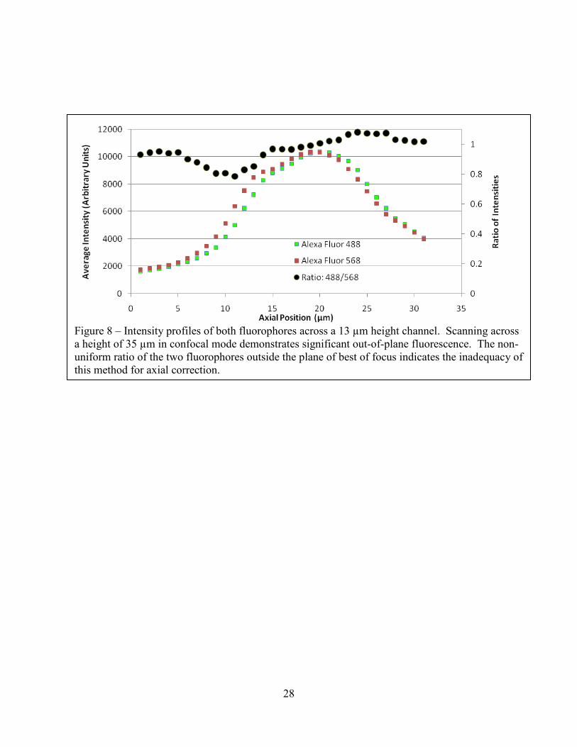
28

Figure 8 – Intensity profiles of both fluorophores across a 13 µm height channel. Scanning across a height of 35 µm in confocal mode demonstrates significant out-of-plane fluorescence. The non-uniform ratio of the two fluorophores outside the plane of best of focus indicates the inadequacy of this method for axial correction.

29

A) B)

Figure 9 – Finite element model utilized to investigate the effects of cell geometry on the distribution of gradients experienced by the cells. A) At each position a cell, indicated by a small circle, was placed with a probability: Yellow – 20%.; Blue – 40%; Red – 70%; Green – 40%. B) 200 cells of each of three relative cell heights were analyzed to demonstrate the shift in average gradient and the dispersion of the gradient

30

experiment. These data demonstrate that both the average gradient that cells see becomes much

steeper and that the distribution becomes much wider as the occlusion increases. In the idealized

case of the cells not occluding the device (0%, Blue), they would be exposed to gradients ranging

from .027%/µm to .068%/µm. If the cells occluded 50% of the height of channels they occupied

(Red), the gradients would range from .037 %/µm to .116 %/µm, whereas the numbers would

change to .033 %/µm to .310 %/µm for 90% occlusion (Blue). The mean and standard deviation

shift accordingly, from a mean of .045 and standard deviation of .010 for the 0% occlusion

condition, to a mean of .071 and standard deviation of .019 for 50% occlusion, and a mean of

.139 with a standard deviation of .066 for the 90% occlusion condition. The steeper average

gradient results from the lower effective diffusivity across highly occluded regions of the device,

while the dispersion of gradients results from the distorting effect of cells on surrounding

regions.

While it is possible that cells can distort gradients significantly, the modeling process

suggests two factors that can potentially minimize the effect. By increasing the aspect ratio of the

device, the percent occlusion will drop accordingly, shifting the gradient distribution towards the

idealized zero cell thickness case. The biology of the cell motility process can also be helpful;

since many cells spread across the substrate before becoming motile, they often occlude less

volume than immediately after loading. To simulate this, we first considered a set of cells that

have occluded the device at 50% of the channel height until time τ/2. Since flattened cells can

spread to a thickness of as little as 1-2 µm, we then allowed the cells to flatten and occlude only

10% of the channel height. In Figure 10 we examine the gradients encountered by a population

of 200 cells at the initial time point of spreading and over the course of a further τ/2. The average

gradient encountered by the cells decreases rapidly after allowing for cell spreading; the mean

31

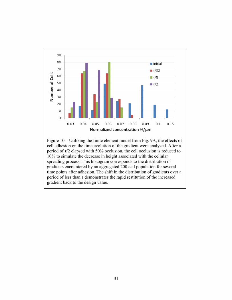
Figure 10 – Utilizing the finite element model from Fig. 9A, the effects of cell adhesion on the time evolution of the gradient were analyzed. After a period of τ/2 elapsed with 50% occlusion, the cell occlusion is reduced to 10% to simulate the decrease in height associated with the cellular spreading process. This histogram corresponds to the distribution of gradients encountered by an aggregated 200 cell population for several time points after adhesion. The shift in the distribution of gradients over a period of less than τ demonstrates the rapid restitution of the increased gradient back to the design value.

32

falls from .070 to .048 within the first τ/32, and then decreases more gradually to .0474 after τ/8

and .040 after τ/2. The variation of the gradients encountered by the cells follows a similar

pattern, declining rapidly from .019 to .012 after τ/32 and then slowly approaching .010 at τ/2.

The rapid adjustment of the gradient is a consequence of the relative scale of the cells. Since the

gradient recovery process is a function of diffusion, which varies as 1/L2, equilibration along the

length of the cell can occur more rapidly than gradient development across the entire bridge.

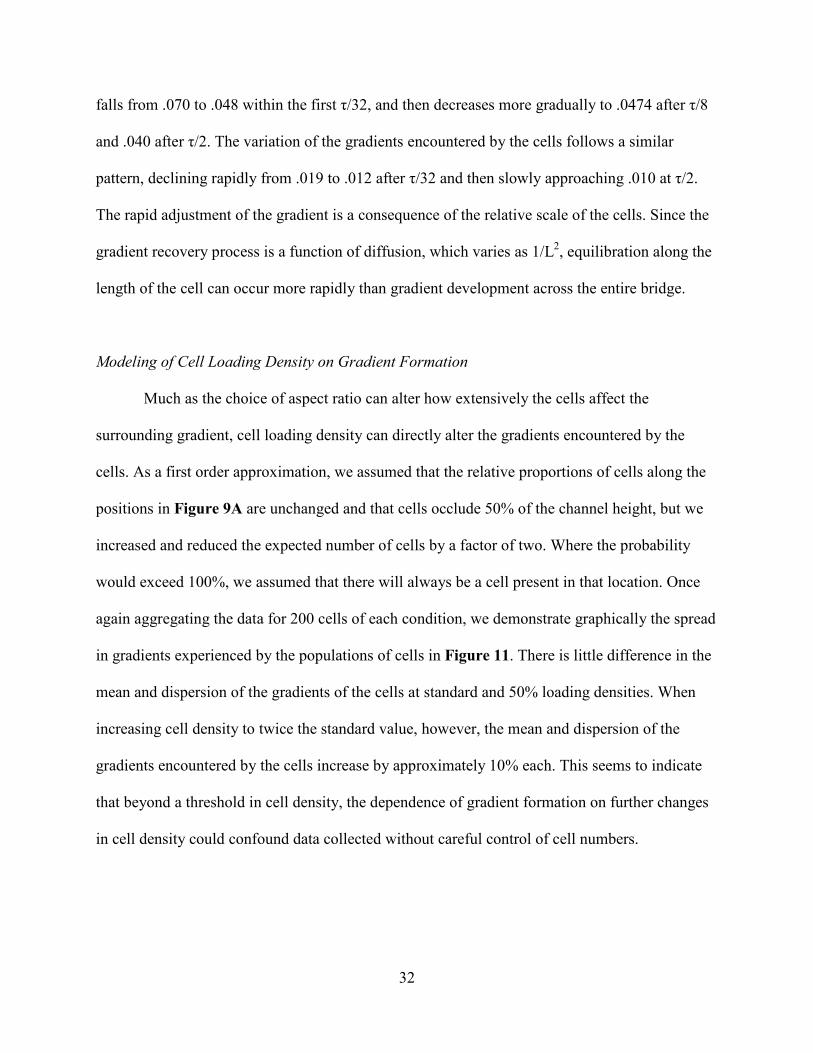
Modeling of Cell Loading Density on Gradient Formation

Much as the choice of aspect ratio can alter how extensively the cells affect the

surrounding gradient, cell loading density can directly alter the gradients encountered by the

cells. As a first order approximation, we assumed that the relative proportions of cells along the

positions in Figure 9A are unchanged and that cells occlude 50% of the channel height, but we

increased and reduced the expected number of cells by a factor of two. Where the probability

would exceed 100%, we assumed that there will always be a cell present in that location. Once

again aggregating the data for 200 cells of each condition, we demonstrate graphically the spread

in gradients experienced by the populations of cells in Figure 11. There is little difference in the

mean and dispersion of the gradients of the cells at standard and 50% loading densities. When

increasing cell density to twice the standard value, however, the mean and dispersion of the

gradients encountered by the cells increase by approximately 10% each. This seems to indicate

that beyond a threshold in cell density, the dependence of gradient formation on further changes

in cell density could confound data collected without careful control of cell numbers.

33

Figure 11 – Utilizing the finite element model from Fig. 9A, the effects of cell loading density on the distribution of gradients encountered by the cells were analyzed. Cell loading density was halved and doubled by adjusting the probabilities mentioned in Fig. 9 while maintaining a relative cell height of 50% occlusion.

34

Discussion

Representative Chemotaxis Device

While the theoretical underpinnings and biological significance of this device are

discussed elsewhere, the motivations for the chosen system are presented briefly. The challenges

of developing a precise, quantifiable chemotactic system have been taken on by a multitude of

microfluidic researchers, resulting in many question-specific systems [40]. Despite the

applicability and potential impact of these systems to biological research, many biologists lack

access to a collaborating microfluidics laboratory and rely on older in vitro systems such as the

Boyden chamber. While this system provides a porous substrate for migration, read-out is

traditionally done by allowing cells to migrate for a pre-determined time and then counting the

number of cells that are on either side of the membrane. Much required information cannot be

obtained, for example, dynamic information on cell motility; instead, one simply counts the

number of cells that cross the filter in a particular time interval, and it is not possible to

determine if there are multiple cellular phenotypes present such as a mixed population of fast-

and slow-migrating cells. Finally, the time frame of migration in the membrane may not be

physiologically relevant and any dispersion in the sizes of the pores in the membrane could skew

the results of the assay [41].

The PDMS system diagrammed in Figure 1 has regular structures produced to a tight

tolerance, is optically transparent and is amenable to high-throughput assessment of chemotaxis

by established automated nuclei counting methods [42]. This system also allows for the

continuous imaging and quantification of the cell actually undergoing the chemotaxis process in

this pore-like environment. Four experiments can be conducted within a single device,

35

corresponding to the four “bridges” connecting the reservoirs. Minor changes to device geometry

allow for each of these bridges to provide a different gradient. Since soft lithography minimizes

any variation in post spacing, the confounding factor of pore size in the Boyden chamber is

eliminated. This device also avoids the flow-based artifacts on cell motility that may be

associated with pressures across macro-scale devices or that may be present in active gradient

generators.

Simultaneous application in our device of a chemical stimulus by the gradient and

mechanical stimuli by the posts will help elucidate effects of the physical environment on

behaviors otherwise treated as purely chemotactic responses [43]. Post structures, or the

equivalent in similar systems, can provide three-dimensional constraints that mimic cellular

microenvironments, constrain cells of a certain size or stiffness, or serve as surfaces for

functionalization with molecules that affect cell adhesion or cellular traction forces. The

chemical and mechanical stimuli that are provided by the system may not be independent,

however, and it becomes important to analyze their interdependence through modeling and

empirical analysis. Cells self-sort in the system based on their ability to invade or migrate while

responding to a combination of cues. This will prove to be a valuable assay and separation

method since, for example, heterogeneity in cancerous cell populations is often reflected by

differences in cellular motility [44, 45]. In summary, three-dimensional chemotaxis systems of

this type will be important to exploring the integrated response of cells in a more life-like

environment, but they also raise the need for a rigorous analysis of distortion in the gradient due

to cells and device geometry.

36

Effects of Device Microstructure on Gradient Formation

When traversing a row of posts, the cross-sectional area in the xy plane of the

microfluidic channels for gradient formation is at a minimum, and the gradient is nearly twice as

steep. This has several consequences for our system. It is reasonable to treat the gradient as

pseudo-stable in time because the spatial variation is significantly greater than the dependence of

the gradient on the passage of time during the length of biologically relevant experiments. In

conducting assays with this system, however, it will be important to note that the behavior of

cells in the regions of the post cannot be attributed solely to mechanical cues since the gradient

also varies. Since this component of the model is conducted in two dimensions by considering

only the obstruction that the PDMS posts provide in the xy plane, the effect is independent of

channel height. If this spatial variation was of concern to the experimenter, the xy footprint of the

posts, the post spacing, or the height of the posts in z could be altered to reduce the spatial

dependence of gradient steepness.

While this model, based on simple Fickian diffusion, demonstrates variation of the

gradient of over a factor of two along the length of the bridge, an unwary experimenter looking

only at concentration profiles in a microfluidic device may easily miss the effect. For example, if

data taken from this model are analyzed under the assumption of a perfectly linear gradient, the

absolute value of the resulting correlation coefficient would be >0.99. Without the use of

complementary analytical and computational tools, incorrect expectations of gradient shape

could easily lead to inaccurate conclusions.

Consequences of High Fluorophore Concentration and the Use of Multiple Fluorophores

Before attempting to use a multi-color correction method to address the problems

described above, we must determine what effects the use of multiple fluorophores will have on

37

the quantification process. In the basic case of exciting a single fluorophore at low

concentrations, an experimenter can expect an effectively linear relationship between

fluorophore concentration and emission intensity [14]. This linear relationship, however, is based

on several assumptions that must be re-analyzed in the context of the multi-dye two- and three-

dimensional imaging methods presented here. When light of the exciting wavelength passes

through a sample, it is being absorbed and dissipated throughout according to the Beer-Lambert

Law. Because of this absorption, the amount of light available to excite fluorophores decreases

throughout the thickness of the sample. As a result, a collection of fluorophores farther from the

light source would emit correspondingly less total fluorescence. The height-dependent

absorption would interfere with the linearity of the relationship between concentration and

fluorescence intensity since the loss of light through the sample would be more significant at

higher concentrations. High concentrations can also lead to quenching in which excited

fluorophores will lose energy by thermal processes instead of by emitting a detectable photon

[14]. Since absorption reduces the illumination as a function of height through the sample,

attempts to measure gradients in three dimensions would be confounded. At low enough

concentrations, however, a negligible amount of light is absorbed through the entire thickness of

the sample. In this case, assuming a linear relationship between concentration and recorded

intensity would be reasonable, and concentration profiles could be derived axially through any

type of optical sectioning.

We also consider the effects of cross-talk between the fluorophores on linear response.

Even with optimized filters for excitation, both fluorophores will absorb light at both of the

excitation wavelengths since the excitation process follows a spectral absorption curve. Since we

showed that even at its peak absorbance neither fluorophore will absorb more than 2% of the

38

illuminating light, we do not need to worry about attenuation of one fluorophore’s excitation by

the other. To determine whether either fluorophore is being significantly excited at the other’s

wavelength, we compared the corresponding absorption spectra (Figure 4). At an excitation

wavelength of 488 nm, the Alexa Fluor 568 is only 3% as absorptive as the Alexa Fluor 488. At

an excitation wavelength of 568 nm, the effect is a bit more pronounced with a cross absorption

of 11%. The contribution to bleed-through, however, is even lower than these values since the

emission filters are also chosen to be specific for the fluorophore of interest. This analysis does

raise the point, however, that at very disparate concentrations bleed-through is possible, and the

existence of a second fluorophore acts to raise the limit of detection of the first. In conclusion,

attention should be paid to ensure that the use of multiple fluorophores does not introduce new

aberrations that overcome the potential advantages of the ratiometric method.

Quantification of Fluorescence Intensity through Ratiometric Image Correction

In a relatively simple architecture like the two-layer device analyzed in this work, the

concentration gradients could be analyzed piecewise to obtain meaningful quantitative data as

long as the experimenter is willing to make assumptions about concentration continuity at height

boundaries. In microfluidic systems with more complex geometries or sources at different

heights, however, the dependence of intensity on channel height might preclude quantification.

While fluorescence microscopy is often idealized to the interrogation of a single plane of the

sample, the fact that microscope components will project cones of illumination and collection

onto a single measured pixel becomes relevant in this multi-height situation. Fluorophore

molecules above and below the plane of interest are illuminated, if not as efficiently as those on

the focal plane. Similarly, light from any plane outside of the focal plane is minimal, but

39

summation across the height of the collection cone becomes significant enough to cause the

variation noted in Figure 5 when utilizing the single-color flat-field correction.

We suspect two related factors contributed to the shadowing effect noted in Figure 6.

The value that is recorded for a single pixel on the CCD camera, as mentioned above,

corresponds to an illumination and collection cone generated by the objective. Depending on the

numerical aperture, shadowed regions will have portions of these cones obstructed by adjacent

posts, reducing the total intensity collected. The refraction index mismatches at interfaces may

also lead to light being improperly trapped and redirected in the PDMS in the same manner as an

optical fiber directs light, an effect known as light-piping. While this effect is actually utilized in

on-chip optical elements, to our knowledge, standard quantitative imaging methods are not

available to correct for this loss [46].

Since the microtopography of the device has such a drastic effect on the illumination and

read-out of a field of view, we evaluated the concept of a field-specific ratiometric correction in

this work. Like existing ratiometric methods for quantifying intracellular calcium concentration

[34], this process provides a numerical correction for differences in the path length and

illumination throughout a three-dimensional sample. Unlike existing methods, however, we

cannot rely on both a measurement and reference signal from a single fluorophore, so we

introduce a uniformly distributed reference molecule. By no longer constraining ourselves to the

subset of fluorophores that provide multiple read-out wavelengths, we can apply the ratiometric

methodology in a more flexible way. Both the corrective capabilities indicated in Figures 5E

and 6E and the flexibility of the method indicate its potential for quantifying emission variation

in topographies that confound traditional flat-field correction. It will also be worthwhile to

determine whether there are chromatic aberrations associated with the PDMS-water interface.

40

Potential of Ratiometric Methods for the Study of Partitioning Effects

The ratiometric imaging process also allows us to explore the possibility of the

partitioning of molecules into the surrounding PDMS. Many small hydrophobic molecules, such

as organic pollutants, affect cell behavior but may be difficult to study in this format because of

partitioning into PDMS structures [47]. While both molecules used in this experiment are too

large and hydrophilic to partition into the surrounding polymer, this process could be repeated

with a reference flurophore that cannot diffuse into the material and a second fluorophore with

an unknown capacity to partition. A gradient of intensity within the corrected image of the posts

would imply that the signal within the posts is actually a result of partitioning instead of a light-

piping related artifact. The negative control case of two large fluorophore molecules would also

have to be conducted, however, to distinguish the possibilities of light-piping, chromatic

aberrations within the device, and small molecule partitioning.

Ratiometric Correction for the Measurement of Gradients along the Optical Axis

There may be several factors that lead to these non-uniform shifts in the z direction noted

with respect to Figure 8. For example, incomplete correction of the chromatic aberration of the

imaging system could contribute to the observed shift in z. While the imaging system may be

color-corrected for the plane of best focus, it seems under- and over-corrected on either side.

Any imperfection in the optics for the two laser colors would also contribute to the observed

behavior. Finally, both the refractive index of the water and PDMS components of the sample

show a dependence on light wavelength over the range we utilize [48, 49]. As a consequence,

light of each wavelength will behave differently with increasing depth into the sample,

confounding our attempts at quantitatively analyzing gradient formation along the optical z axis.

41

CHAPTER III

CONCLUSIONS AND FUTURE DIRECTIONS

Microfluidic devices have been making inroads as an experimental platform despite the

difficulty of developing universal solutions and translating engineering advances into biological

tools. Construction of a system on these scales has great potential for making chemotaxis assays

more precise, reproducible, and amenable to analytic characterization. As researchers begin to

investigate the integrated responses of cells by using the micron feature sizes of microfluidics to

create a controlled microenvironment for cells, they will need new tools to eliminate

confounding variables and accurately quantify experimental data.

In this work, we considered gradient formation in a microfluidic device with a complex

topography and no replenishment of the chemoattractant. The effects of device geometry on local

gradient formation were significant, and for this particular device we demonstrated that gradients

in the regions of posts were twice as steep as those in unobstructed regions. As we attempted to

empirically quantify this spatial dependence on gradient formation, we were confounded by the

effects of varying channel heights and of PDMS structures on quantitative fluorescence

measurements.

To correct for differences in light path and light-piping effects in the proximity of

structures, we utilized a novel ratiometric correction employing a second uniform reference

fluorophore. While the ratiometric concept is not new, it has traditionally been limited to a single

dye method for specific applications such as intracellular calcium measurement. To generalize

this system for quantification of concentration gradients within our microfluidic devices, we

42

introduced a second fluorophore. We examined the possibility of cross-talk between the

fluorophores, determining that deviations from linearity should be negligible for the fluorophore

concentrations utilized. The ratiometric process proved an effective, though not complete,

solution for these two categories of fluorescence differences. We also demonstrated agreement of

experimental data with the basic Fickian models we proposed. Through further optimization, we

believe that this method could allow for more accurate quantification of fluorescence in the

complex microstructures that are becoming common in microfluidic design. We considered this

method for quantifying fluorescence in three dimensions in conjunction with confocal

microscopy. In our experience, different fluorophores demonstrate different dependencies on

height, precluding the use of a reference fluorophore as a way of correcting for differences in

illumination across the height of the sample.

By supplementing the ratiometric technique with an algorithm that takes into account the

differences between fluorophores, it may be possible to overcome the difficulty associated with

measuring gradients in the z axis. The ratiometric correction method could, for example, be used

in conjunction with two-photon microscopy to minimize the contribution of out-of-plane

components [50]. In microfluidic devices with high enough fluorophore concentrations to

introduce cross-talk between the fluorophores, a linear un-mixing system could also allow for

distinguishing the otherwise convoluted signals [51]. There is still significant work to be done to

address the potential causes mentioned above for the variation between the fluorophores as a

function of height. For example, illumination could be done in a broadband manner to eliminate

alignment issues between lasers. This would require an appropriate filter set or spectrometer for

separation of the emission wavelengths. Similarly, samples could be chosen with minimal

dispersion in the visible wavelengths to eliminate that as a cause of error.

43

In the last component of this work, we considered the effect that the cells themselves

have on gradient formation. Neglecting active remodeling of the gradient through cellular

metabolism or production, we primarily analyzed the effect of cells on device geometry. By

probabilistically inserting cell-shaped occlusions into the original finite element model of the

system, we were able to examine how aspect ratio and cell loading density affected local

gradients in the device. There is no single gradient associated with a set of device parameters,

however, so we present data in terms of distributions of gradients. We showed that the

distribution will shift upward in mean value and become more disperse as the effective cell

height, or occlusion, increases. Fortunately for the examination of motile cells, the adhesion and

flattening of cells are followed by rapid reduction in gradient steepness. We also demonstrated

that the mean gradient that an average cell encounters will be a direct function of cell loading

density. These conclusions have consequences for explaining the heterogeneity of cell behavior

in microfluidic chemotaxis assays.

The approach we take in this work will become increasingly relevant as more

interdisciplinary teams utilize microfluidic devices as a platform for asking biological questions

that require precise measurements. While many applications can safely dismiss so-called optical

edge effects near interfaces of substrate and fluid, the increasing demand for mimicking the

entire cellular microenvironment will necessitate the inclusion of mechanical cues. If

micropatterned structures are used to present these cues, accurate imaging in the proximity of

these structures may prove to be important. By considering complementary methods for

modeling and quantifying gradient formation in these complex systems, we present a suite of

tools for the rational design and evaluation of gradient formation in microfluidics with features

that have cell-sized dimensions.

44

REFERENCES

[1] S. K. Sia, and G. M. Whitesides, “Microfluidic devices fabricated in Poly(dimethylsiloxane) for biological studies,” Electrophoresis, 24(21), 3563-3576 (2003).

[2] T. M. Squires, and S. R. Quake, “Microfluidics: Fluid physics at the nanoliter scale,”

Reviews of Modern Physics, 77(3), 977-1026 (2005). [3] D. J. Beebe, G. A. Mensing, and G. M. Walker, “Physics and applications of

microfluidics in biology,” Annual Review of Biomedical Engineering, 4, 261-286 (2002). [4] G. M. Walker, H. C. Zeringue, and D. J. Beebe, “Microenvironment design

considerations for cellular scale studies,” Lab on a Chip, 4(2), 91-97 (2004). [5] J. P. Wikswo, A. Prokop, F. Baudenbacher et al., “Engineering challenges of BioNEMS:

the integration of microfluidics, micro- and nanodevices, models and external control for systems biology,” Iee Proceedings-Nanobiotechnology, 153(4), 81-101 (2006).

[6] N. L. Jeon, S. K. W. Dertinger, D. T. Chiu et al., “Generation of solution and surface

gradients using microfluidic systems,” Langmuir, 16(22), 8311-8316 (2000). [7] D. Irimia, D. A. Geba, and M. Toner, “Universal microfluidic gradient generator,”

Analytical Chemistry, 78(10), 3472-3477 (2006). [8] S. Faley, K. Seale, J. Hughey et al., “Microfluidic platform for real-time signaling

analysis of multiple single T cells in parallel,” Lab on a Chip, 8(10), 1700-1712 (2008). [9] Y. Wang, T. Mukherjee, and Q. Lin, “Systematic modeling of microfluidic concentration

gradient generators,” Journal of Micromechanics and Microengineering, 16(10), 2128-2137 (2006).

[10] B. R. Gorman, and J. P. Wikswo, “Characterization of transport in microfluidic gradient

generators,” Microfluidics and Nanofluidics, 4(4), 273-285 (2008). [11] A. Khademhosseini, R. Langer, J. Borenstein et al., “Microscale technologies for tissue

engineering and biology,” Proceedings of the National Academy of Sciences of the United States of America, 103(8), 2480-2487 (2006).

[12] J. J. Norman, J. M. Collins, S. Sharma et al., “Microstructures in 3D biological gels affect

cell proliferation,” Tissue Engineering Part A, 14(3), 379-390 (2008). [13] U. Haessler, Y. Kalinin, M. A. Swartz et al., “An agarose-based microfluidic platform

with a gradient buffer for 3D chemotaxis studies,” Biomedical Microdevices, 11(4), 827-

45

835 (2009). [14] D. Murphy, [Fundamentals of Light Microscopy and Electronic Imaging] Wiley-Liss,

New York(2001). [15] C. Beta, T. Frohlich, H. U. Bodeker et al., “Chemotaxis in microfluidic devices - a study

of flow effects,” Lab on a Chip, 8(7), 1087-1096 (2008). [16] S. Li, N. F. Huang, and S. Hsu, “Mechanotransduction in endothelial cell migration,”

Journal of Cellular Biochemistry, 96(6), 1110-1126 (2005). [17] M. Iiizumi, W. Liu, S. K. Pai et al., “Drug development against metastasis-related genes

and their pathways: A rationale for cancer therapy,” Biochimica Et Biophysica Acta-Reviews on Cancer, 1786(2), 87-104 (2008).

[18] P. Devreotes, “Dictyostelium-discoideum - A model system for cell-cell interactions in

development,” Science, 245(4922), 1054-1058 (1989). [19] P. Devreotes, and C. Janetopoulos, “Eukaryotic chemotaxis: Distinctions between

directional sensing and polarization,” Journal of Biological Chemistry, 278(23), 20445-20448 (2003).

[20] S. Boyden, “The chemotactic effect of mixtures of antibody and antigen on

polymorphonuclear leucocytes,” J. Exp. Med., 115(3), 453-466 (1962). [21] S. H. Zigmond, and S. J. Sullivan, “Sensory adaptation of leukocytes to chemotactic

peptides,” Journal of Cell Biology, 82(2), 517-527 (1979). [22] D. Zicha, G. A. Dunn, and A. F. Brown, “A new direct-viewing chemotaxis chamber,”

Journal of Cell Science, 99, 769-775 (1991). [23] Y. X. Liu, J. Q. Sai, A. Richmond et al., “Microfluidic switching system for analyzing

chemotaxis responses of wortmannin-inhibited HL-60 cells,” Biomedical Microdevices, 10(4), 499-507 (2008).

[24] K. Lee, C. Kim, B. Ahn et al., “Generalized serial dilution module for monotonic and

arbitrary microfluidic gradient generators,” Lab on a Chip, 9(5), 709-717 (2009). [25] G. M. Walker, J. Q. Sai, A. Richmond et al., “Effects of flow and diffusion on

chemotaxis studies in a microfabricated gradient generator,” Lab on a Chip, 5(6), 611-618 (2005).

[26] H. K. Wu, B. Huang, and R. N. Zare, “Generation of complex, static solution gradients in

microfluidic channels,” Journal of the American Chemical Society, 128(13), 4194-4195 (2006).

46

[27] A. Shamloo, N. Ma, M. M. Poo et al., “Endothelial cell polarization and chemotaxis in a microfluidic device,” Lab on a Chip, 8(8), 1292-1299 (2008).

[28] Y. Du, J. Shim, M. Vidula et al., “Rapid generation of spatially and temporally

controllable long-range concentration gradients in a microfluidic device,” Lab on a Chip, 9(6), 761-767 (2009).

[29] S. Li, J. L. Guan, and S. Chien, “Biochemistry and biomechanics of cell motility,”

Annual Review of Biomedical Engineering, 7, 105-150 (2005). [30] R. G. Thakar, M. G. Chown, A. Patel et al., “Contractility-dependent modulation of cell

proliferation and adhesion by microscale topographical cues,” Small, 4(9), 1416-1424 (2008).

[31] A. Brock, E. Chang, C. C. Ho et al., “Geometric determinants of directional cell motility

revealed using microcontact printing,” Langmuir, 19(5), 1611-1617 (2003). [32] B. Mosadegh, C. Huang, J. W. Park et al., “Generation of stable complex gradients across

two-dimensional surfaces and three-dimensional gels,” Langmuir, 23(22), 10910-10912 (2007).

[33] G. M. Walker, and D. J. Beebe, “A passive pumping method for microfluidic devices,”

Lab on a Chip, 2(3), 131-134 (2002). [34] A. Takahashi, P. Camacho, J. D. Lechleiter et al., “Measurement of intracellular

calcium,” Physiological Reviews, 79(4), 1089-1125 (1999). [35] M. S. Williams, K. J. Longmuir, and P. Yager, “A practical guide to the staggered

herringbone mixer,” Lab on a Chip, 8(7), 1121-1129 (2008). [36] J. C. McDonald, D. C. Duffy, J. R. Anderson et al., “Fabrication of microfluidic systems

in poly(dimethylsiloxane),” Electrophoresis, 21(1), 27-40 (2000). [37] A. F. Mills, [Basic Heat and Mass Transfer] Prentice Hall, Los Angeles(1999). [38] Z. H. Liang, N. Chiem, G. Ocvirk et al., “Microfabrication of a planar absorbance and

fluorescence cell for integrated capillary electrophoresis devices,” Analytical Chemistry, 68(6), 1040-1046 (1996).

[39] R. Sjoback, J. Nygren, and M. Kubista, “Absorption and fluorescence properties of

fluorescein,” Spectrochimica Acta Part a-Molecular and Biomolecular Spectroscopy, 51(6), L7-L21 (1995).

[40] T. M. Keenan, and A. Folch, “Biomolecular gradients in cell culture systems,” Lab on a

Chip, 8(1), 34-57 (2008).

47

[41] G. Cinamon, and R. Alon, “A real time in vitro assay for studying leukocyte transendothelial migration under physiological flow conditions,” Journal of Immunological Methods, 273(1-2), 53-62 (2003).

[42] H. Ancin, B. Roysam, T. E. Dufresne et al., “Advances in automated 3-D image analysis

of cell populations imaged by confocal microscopy,” Cytometry, 25(3), 221-234 (1996). [43] A. K. McNulty, M. Schmidt, T. Feeley et al., “Effects of negative pressure wound

therapy on fibroblast viability, chemotactic signaling, and proliferation in a provisional wound (fibrin) matrix,” Wound Repair and Regeneration, 15(6), 838-846 (2007).

[44] M. Harris, E. Kim, B. Weidow et al., “Migration of isogenic cell lines quantified by

dynamic multivariate analysis of single-cell motility.,” Cell Adh Migr, 2(2), 127-36 (2008).

[45] E. LaTulippe, J. Satagopan, A. Smith et al., “Comprehensive gene expression analysis of

prostate cancer reveals distinct transcriptional programs associated with metastatic disease,” Cancer Research, 62(15), 4499-4506 (2002).

[46] D. A. Chang-Yen, R. K. Eich, and B. K. Gale, “A monolithic PDMS waveguide system

fabricated using soft-lithography techniques,” Journal of Lightwave Technology, 23(6), 2088-2093 (2005).

[47] J. H. Kwon, T. Wuethrich, P. Mayer et al., “Dynamic permeation method to determine

partition coefficients of highly hydrophobic chemicals between poly(dimethylsiloxane) and water,” Analytical Chemistry, 79(17), 6816-6822 (2007).

[48] A. N. Bashkatov, and E. A. Genina, “Water refractive index in dependence on

temperature and wavelength: a simple approximation,” Proceedings of the SPIE - The International Society for Optical Engineering, 5068(1), 393-5 (2003).

[49] F. Schneider, J. Draheirn, R. Kamberger et al., “Process and material properties of

polydimethylsiloxane (PDMS) for Optical MEMS,” Sensors and Actuators a-Physical, 151(2), 95-99 (2009).

[50] C. Xu, W. Zipfel, J. B. Shear et al., “Multiphoton fluorescence excitation: New spectral

windows for biological nonlinear microscopy,” Proceedings of the National Academy of Sciences of the United States of America, 93(20), 10763-10768 (1996).

[51] T. Zimmermann, J. Rietdorf, A. Girod et al., “Spectral imaging and linear un-mixing

enables improved FRET efficiency with a novel GFP2-YFP FRET pair,” Febs Letters, 531(2), 245-249 (2002).