of Transportallon Errata...Volume Ⅰ is the final report, and Volume Ⅱthrough Volume Ⅹconsist of Appendix A through Appendix Ⅰ. Any reference to a volume in this series will

0 U.S. Department of Transportallon Federal Highway Administration

Errata

Date: April 17, 2019

Issuing Office: Federal Highway Administration—Office of Research,

Development, and Technology

Address: Turner-Fairbank Highway Research Center, 6300 Georgetown

Pike, McLean, VA 22101

Name of Document: Analysis Procedures for Evaluating Superheavy Load Movement

on Flexible Pavements, Volume I: Final Report

FHWA Publication No.: FHWA-HRT-18-049

The following changes were made to the document after publication on the Federal Highway

Administration website:

Location Incorrect Values Corrected Values

TECHNICAL

REPORT

DOCUMENTATION

PAGE, Box 15

Nadarajah Sivaneswaran

(HRDI-20; ORCID: 0000-0002-

3525-9165), Office of

Infrastructure Research and

Development, Turner-Fairbank

Highway Research Center,

served as the Contracting

Officer’s Representative.

Nadarajah Sivaneswaran

(HRDI-20; ORCID:

0000-0003-0287-664X), Office

of Infrastructure Research and

Development, Turner-Fairbank

Highway Research Center,

served as the Contracting

Officer’s Representative.

US. Deportment o1 Transportation

Federal Highway Administration

Analysis Procedures for Evaluating Superheavy Load Movement on Flexible Pavements, Volume I: Final Report PUBLICATION NO. FHWA-HRT-18-049 OCTOBER 2018

Research, Development, and Technology Turner-Fairbank Highway Research Center 6300 Georgetown Pike McLean, VA 22101-2296

FOREWORD

The movement of superheavy loads (SHLs) on the Nation’s highways is an increasingly

common, vital economic necessity for many important industries, such as chemical, oil,

electrical, and defense. Many superheavy components are extremely large and heavy (gross

vehicle weights in excess of a few million pounds), and they often require specialized trailers and

hauling units. At times, SHL vehicles have been assembled to suit the load being transported,

and therefore, the axle configurations have not been standard or consistent. Accommodating

SHL movements without undue damage to highway infrastructure requires the determination of

whether the pavement is structurally adequate to sustain the SHL movement and protect any

underground utilities. Such determination involves analyzing the likelihood of instantaneous or

rapid load-induced shear failure of the pavement structure.

The goal of this project was to develop a comprehensive analysis process for evaluating SHL

movement on flexible pavements. As part of this project, a comprehensive mechanistic-based

analysis approach consisting of several analysis procedures was developed for flexible pavement

structures and documented in a 10-volume series of Federal Highway Administration reports—a

final report and 9 appendices.(1–9) This is Analysis Procedures for Evaluating Superheavy Load

Movement on Flexible Pavements, Volume I: Final Report, which presents a summary of the

analysis procedures developed to address the critical factors associated with SHL movement on

flexible pavements. This report is intended for use by highway agency pavement engineers

responsible for assessing the structural adequacy of pavements in the proposed route and

identifying mitigation strategies, where warranted, in support of the agency’s response to SHL-

movement permit requests.

Cheryl Allen Richter, Ph.D., P.E.

Director, Office of Infrastructure

Research and Development

Notice

This document is disseminated under the sponsorship of the U.S. Department of Transportation

(USDOT) in the interest of information exchange. The U.S. Government assumes no liability for

the use of the information contained in this document.

The U.S. Government does not endorse products or manufacturers. Trademarks or

manufacturers’ names appear in this report only because they are considered essential to the objective of the document.

Quality Assurance Statement

The Federal Highway Administration (FHWA) provides high-quality information to serve

Government, industry, and the public in a manner that promotes public understanding. Standards

and policies are used to ensure and maximize the quality, objectivity, utility, and integrity of its

information. FHWA periodically reviews quality issues and adjusts its programs and processes to

ensure continuous quality improvement

I

I I I

TECHNICAL REPORT DOCUMENTATION PAGE 1. Report No.

FHWA-HRT-18-049

2. Government Accession No. 3. Recipient’s Catalog No.

4. Title and Subtitle

Analysis Procedures for Evaluating Superheavy Load Movement on

Flexible Pavements, Volume I: Final Report

5. Report Date

October 2018

6. Performing Organization Code

7. Author(s)

Elie Y. Hajj (ORCID: 0000-0001-8568-6360), Raj V. Siddharthan

(ORCID: 0000-0002-3847-7934), Hadi Nabizadeh (ORCID: 0000-

0001-8215-1299), Sherif Elfass (ORCID: 0000-0003-3401-6513),

Mohamed Nimeri (ORCID: 0000-0002-3328-4367), Seyed Farzan

Kazemi (ORCID: 0000-0003-2313-4995), Dario Batioja-Alvarez

(0000-0002-1094-553X), and Murugaiyah Piratheepan (ORCID:

0000-0002-3302-4856)

8. Performing Organization Report No.

WRSC-UNR-201710-01

9. Performing Organization Name and Address

Department of Civil and Environmental Engineering

University of Nevada

1664 North Virginia Street

Reno, NV 89557

10. Work Unit No.

11. Contract or Grant No.

DTFH61-13-C-00014

12. Sponsoring Agency Name and Address

Office of Research, Development, and Technology

Federal Highway Administration

6300 Georgetown Pike

McLean, VA 22101

13. Type of Report and Period Covered

Final Report; August 2013–July 2018

14. Sponsoring Agency Code

HRDI-20

15. Supplementary Notes

Nadarajah Sivaneswaran (HRDI-20; ORCID: 0000-0003-0287-664X*), Office of Infrastructure Research and

Development, Turner-Fairbank Highway Research Center, served as the Contracting Officer’s Representative.

16. Abstract

The movement of superheavy loads (SHLs) has become more common over the years, since it is a vital

necessity for many important industries, such as chemical, oil, electrical, and defense. SHL hauling units are

much larger in size and weight compared to the standard trucks. SHL gross vehicle weights may be in excess of

a few million pounds, so they often require specialized trailers and components with nonstandard spacing

between tires and axles. Accommodating SHL movements requires the determination of whether the pavement

is structurally adequate and involves the analysis of the likelihood of instantaneous or rapid load-induced shear

failure. In this study, a comprehensive mechanistic-based methodology consisting of the following procedures

was developed: segmentation of an SHL vehicle for analysis, subgrade bearing failure analysis, sloped-shoulder

failure analysis, buried utility risk analysis, localized shear failure analysis, deflection-based service limit

analysis, and cost allocation analysis. In addition, a comprehensive experimental program that included five full-

scale pavement/soil testing experiments performed at a large-scale box facility was designed and carried out for

the verification and calibration of a number of theoretically based procedures incorporated in the analysis

approach. Supplementary numerical modeling as well as measured data from Accelerated Pavement Testing

facilities provided additional verification of the procedures adopted in this study. The analysis procedures

developed were then implemented into a user-friendly software package, SuperPACK (Superheavy Load

Pavement Analysis PACKage), to evaluate SHL movements on flexible pavements. This report presents a

summary of the analysis procedures developed for evaluating SHL movement on flexible pavements. Further (1–9) details of these procedures are presented in a series of stand-alone appendices (volumes Ⅱ through Ⅹ).

17. Key Words

Superheavy load, flexible pavement, nondestructive

testing, ultimate failure, buried utility, service limit,

cost allocation

18. Distribution Statement

No restrictions. This document is available through the

National Technical Information Service, Springfield,

VA 22161.

http://www.ntis.gov

19. Security Classif. (of this report)

Unclassified

20. Security Classif. (of this page)

Unclassified

21. No. of Pages

117

22. Price

N/A

Form DOT F 1700.7 (8-72) Reproduction of completed page authorized.

*Revised 4/17/2019

SI* (MODERN METRIC) CONVERSION FACTORS APPROXIMATE CONVERSIONS TO SI UNITS

Symbol When You Know Multiply By To Find Symbol

LENGTH in inches 25.4 millimeters mm ft feet 0.305 meters m

yd yards 0.914 meters m mi miles 1.61 kilometers km

AREA in

2square inches 645.2 square millimeters mm

2

ft2

square feet 0.093 square meters m2

yd2

square yard 0.836 square meters m2

ac acres 0.405 hectares ha

mi2

square miles 2.59 square kilometers km2

VOLUME fl oz fluid ounces 29.57 milliliters mL

gal gallons 3.785 liters L ft

3 cubic feet 0.028 cubic meters m

3

yd3

cubic yards 0.765 cubic meters m3

NOTE: volumes greater than 1000 L shall be shown in m3

MASS oz ounces 28.35 grams g

lb pounds 0.454 kilograms kgT short tons (2000 lb) 0.907 megagrams (or "metric ton") Mg (or "t")

TEMPERATURE (exact degrees) oF Fahrenheit 5 (F-32)/9 Celsius

oC

or (F-32)/1.8

ILLUMINATION fc foot-candles 10.76 lux lx fl foot-Lamberts 3.426 candela/m

2 cd/m

2

FORCE and PRESSURE or STRESS lbf poundforce 4.45 newtons N

lbf/in2

poundforce per square inch 6.89 kilopascals kPa

APPROXIMATE CONVERSIONS FROM SI UNITS

Symbol When You Know Multiply By To Find Symbol

LENGTHmm millimeters 0.039 inches in

m meters 3.28 feet ft m meters 1.09 yards yd

km kilometers 0.621 miles mi

AREA mm

2 square millimeters 0.0016 square inches in

2

m2 square meters 10.764 square feet ft

2

m2 square meters 1.195 square yards yd

2

ha hectares 2.47 acres ac

km2

square kilometers 0.386 square miles mi2

VOLUME mL milliliters 0.034 fluid ounces fl oz

L liters 0.264 gallons gal m

3 cubic meters 35.314 cubic feet ft

3

m3

cubic meters 1.307 cubic yards yd3

MASS g grams 0.035 ounces oz

kg kilograms 2.202 pounds lbMg (or "t") megagrams (or "metric ton") 1.103 short tons (2000 lb) T

TEMPERATURE (exact degrees) oC Celsius 1.8C+32 Fahrenheit

oF

ILLUMINATION lx lux 0.0929 foot-candles fc cd/m

2candela/m

20.2919 foot-Lamberts fl

FORCE and PRESSURE or STRESS N newtons 0.225 poundforce lbf

kPa kilopascals 0.145 poundforce per square inch lbf/in2

*SI is the symbol for th International System of Units. Appropriate rounding should be made to comply with Section 4 of ASTM E380. e

(Revised March 2003)

ii

ANALYSIS PROCEDURES FOR EVALUATING SUPERHEAVY LOAD MOVEMENT

ON FLEXIBLE PAVEMENTS PROJECT REPORT SERIES

This volume is the first of 10 volumes in this research report series. Volume Ⅰ is the final report,

and Volume Ⅱ through Volume Ⅹ consist of Appendix A through Appendix Ⅰ. Any reference to a

volume in this series will be referenced in the text as “Volume Ⅱ: Appendix A,” “Volume Ⅲ Appendix B,” and so forth. The following list contains the volumes:

Volume Title

Ⅰ Analysis Procedures for Evaluating Superheavy Load

Movement on Flexible Pavements, Volume I: Final Report

Ⅱ Analysis Procedures for Evaluating Superheavy Load

Movement on Flexible Pavements, Volume II: Appendix A,

Experimental Program

Ⅲ Analysis Procedures for Evaluating Superheavy Load

Movement on Flexible Pavements, Volume III: Appendix B,

Superheavy Load Configurations and Nucleus of Analysis

Vehicle

Ⅳ Analysis Procedures for Evaluating Superheavy Load

Movement on Flexible Pavements, Volume IV: Appendix C,

Material Characterization for Superheavy Load Movement

Analysis

Ⅴ Analysis Procedures for Evaluating Superheavy Load

Movement on Flexible Pavements, Volume V: Appendix D,

Estimation of Subgrade Shear Strength Parameters Using

Falling Weight Deflectometer

Ⅵ Analysis Procedures for Evaluating Superheavy Load

Movement on Flexible Pavements, Volume VI: Appendix E,

Ultimate and Service Limit Analyses

Ⅶ Analysis Procedures for Evaluating Superheavy Load

Movement on Flexible Pavements, Volume VII: Appendix F,

Failure Analysis of Sloped Pavement Shoulders

Ⅷ Analysis Procedures for Evaluating Superheavy Load

Movement on Flexible Pavements, Volume VIII: Appendix G,

Risk Analysis of Buried Utilities Under Superheavy Load

Vehicle Movements

Ⅸ Analysis Procedures for Evaluating Superheavy Load

Movement on Flexible Pavements, Volume IX: Appendix H,

Analysis of Cost Allocation Associated with Pavement Damage

Under a Superheavy Load Vehicle Movement

Ⅹ Analysis Procedures for Evaluating Superheavy Load

Movement on Flexible Pavements, Volume X: Appendix I,

Analysis Package for Superheavy Load Vehicle Movement on

Flexible Pavement (SuperPACK)

Report Number

FHWA-HRT-18-049

FHWA-HRT-18-050

FHWA-HRT-18-051

FHWA-HRT-18-052

FHWA-HRT-18-053

FHWA-HRT-18-054

FHWA-HRT-18-055

FHWA-HRT-18-056

FHWA-HRT-18-057

FHWA-HRT-18-058

iii

CHAPTER 1.

CHAPTER 2.

CHAPTER 3.

CHAPTER 4.

TABLE OF CONTENTS

INTRODUCTION ............................................................................................1

1.1. PROBLEM STATEMENT ...........................................................................................1

1.2. OBJECTIVES AND SCOPE OF WORK....................................................................5

1.3. ORGANIZATION OF REPORT .................................................................................6

METHODOLOGY ...........................................................................................7

2.1. SHL ANALYSIS VEHICLE.......................................................................................10

2.1.1. Axle Grouping of SHL Vehicle ...........................................................................10

2.1.2. Nucleus of SHL Analysis Vehicle .......................................................................10

2.2. FLEXIBLE PAVEMENT STRUCTURE..................................................................12

2.2.1. Stiffness Properties of Pavement Layers..............................................................13

2.2.2. SG τmax Properties.................................................................................................13

2.3. ULTIMATE FAILURE ANALYSES ........................................................................20

2.3.1. SG Bearing Failure Analysis................................................................................20

2.3.2. Sloped-Shoulder Failure Analysis........................................................................22

2.4. BURIED UTILITY RISK ANALYSIS ......................................................................25

2.5. SERVICE LIMIT ANALYSES ..................................................................................27

2.5.1. Localized Shear Failure Analysis.........................................................................27

2.5.2. Deflection-Based Service Limit Analysis ............................................................29

2.6. COST ALLOCATION ANALYSIS ...........................................................................31

2.7. MITIGATION STRATEGIES ...................................................................................34

VERIFICATION AND CALIBRATION.....................................................35

3.1. LARGE-SCALE BOX DESCRIPTION ....................................................................36

3.2. VERIFICATION AND CALIBRATION EXERCISE.............................................37

3.2.1. Verification of 3D-Move ENHANCED...............................................................38

3.2.2. Verification of SG τmax Parameters Estimation Procedure...................................45

3.2.3. Determination of SAFShoulder .................................................................................47

3.2.4. Verification of Sloped-Shoulder Failure Analysis Procedure..............................52

3.2.5. Determination of SAFUtility....................................................................................53

3.2.6. Verification of Buried Utility Risk Analysis Procedure ......................................58

SHL CASE STUDIES ....................................................................................61

4.1. SHL ANALYSIS VEHICLES CONFIGURATIONS ..............................................61

4.2. PAVEMENT STRUCTURE AND MATERIAL PROPERTIES............................61

4.3. AXLE GROUPING AND NUCLEUS OF SHL ANALYSIS VEHICLES .............63

4.4. ULTIMATE FAILURE ANALYSES UNDER SHL VEHICLES ..........................65

4.4.1. SG Bearing Failure Analysis................................................................................65

4.4.2. Sloped-Shoulder Failure Analysis Under LA-8T-14 ...........................................66

4.5. BURIED UTILITY RISK ANALYSIS UNDER LA-8T-14.....................................67

4.6. SERVICE LIMIT ANALYSES UNDER SHL VEHICLES ....................................68

4.6.1. Localized Shear Failure Analysis Under SHL Vehicles ......................................68

4.6.2. Deflection-Based Service Limit Analysis Under SHL Vehicles .........................69

4.7. COST ALLOCATION ANALYSIS: LA-12T-16 AND LA-8T-14 ..........................72

4.8. SUMMARY ..................................................................................................................76

iv

CHAPTERS.

CHAPTER 6.

IMPLEMENTATION: SUPERPACK .........................................................79

5.1. ANALYSIS ENGINE: 3D-MOVE ENHANCED......................................................81

5.2. SURFACE PLOTS.......................................................................................................83

5.3. INTERFACE BOND CONDITIONS.........................................................................85

5.4. RUNTIME IMPROVEMENT....................................................................................86

5.5. PREANALYSIS MODULES (A MODULES) ..........................................................87

5.6. ANALYSIS MODULES (B MODULES) ..................................................................87

5.7. SUMMARY ..................................................................................................................92

SUMMARY AND SUGGESTED RESEARCH...........................................95

6.1. SUMMARY AND VALIDATION OF DEVELOPED APPROACH .....................95

6.2. SUGGESTED RESEARCH........................................................................................99

REFERENCES.............................................................................................................................99

v

LIST OF FIGURES

Figure 1. Illustration. Example configuration (LA-8T-14) of a Louisiana-permitted SHL

vehicle (continuous axle configuration) .................................................................................1


vehicle (fragmented axle configuration) ................................................................................2

Figure 3. Illustration. Five-line model for SHL-vehicle simulation—plan view ............................3

Figure 4. Illustration. Five-line model for SHL-vehicle simulation—elevation view.....................3

Figure 5. Illustration. σv distribution within pavement—case 1 ......................................................4



Figure 8. Flowchart. Overall SHL-vehicle analysis methodology ..................................................8

Figure 9. Illustration. Example configuration of a permitted SHL truck in Nevada .....................10

Figure 10. Illustration. Representative nucleus for case No. LA-8T-14........................................12

Figure 11. Flowchart. Estimation of damaged E* for AC layer ....................................................14

Figure 12. Equation. Estimation of E for lean concrete and CTB .................................................18

Figure 13. Equation. Estimation of E for soil cement....................................................................18

Figure 14. Graph. Extrapolation of hyperbolic relationship ..........................................................19

Figure 15. Graph. Estimation of df using linear form of hyperbolic relationship ........................19

Figure 16. Equation. Nonlinear hyperbolic stress–strain relationship of soils ..............................20

Figure 17. Equation. Hyperbolic relationship in linear form.........................................................20

Figure 18. Equation. Meyerhof’s general bearing capacity...........................................................20

Figure 19. Chart. σv distribution on top of the SG under the nucleus (case No. LA-8T-14) .........21

Figure 20. Chart. σv distribution on top of the SG under the nucleus and Aaffected (case No.

LA-8T-14) ............................................................................................................................22

Figure 21. Illustration. Search schemes for failure wedges ...........................................................23

Figure 22. Illustration. Failure wedge with horizontal slip surface and applied forces.................24

Figure 23. Illustration. Failure wedge with inclined slip surface and applied forces ....................24

Figure 24. Equation. FOS against failure for the wedges with inclined slip surface.....................24

Figure 25. Equation. FOS against failure for the wedges with horizontal slip surface .................24

Figure 26. Illustration. Computation of σv at the location of buried utility using 3D-Move

ENHANCED........................................................................................................................26

Figure 27. Illustration. The Drucker–Prager and Mohr–Coulomb yield surfaces .........................27

Figure 28. Graph. Representation of Drucker–Prager failure criterion in the q–p plot .................28

Figure 29. Chart. FOS under SHL-vehicle nucleus .......................................................................29

Figure 30. Chart. FWD load–deflection curve...............................................................................30

Figure 31. Chart. Representation of τmax and applied stresses .......................................................31

Figure 32. Chart. FWD load–SSR curve .......................................................................................31

Figure 33. Flowchart. Overall approach for the estimation of pavement damage and

allocated cost ........................................................................................................................33

Figure 34. Illustration. 3D schematic of large-scale box ...............................................................37

Figure 35. Illustration. Large-scale box experiment No. 1 ............................................................39



Figure 38. Photo. Completed large-scale box test setup for experiment No. 1 .............................40


vi


Figure 41. Graph. Vertical surface displacements measured by LVDT1 in experiment No.

3 at different load levels .......................................................................................................42

Figure 42. Graph. σv measured by TEPC1 in experiment No. 3 at different load levels ...............42

Figure 43. Graph. Measured deflection basin in experiment No. 3...............................................43

Figure 44. Graph. Comparison between 3D-Move calculated deflections and measured

surface deflections in experiment No. 3...............................................................................44

Figure 45. Graph. Comparison between 3D-Move calculated σv and measured σv in

experiment No. 3 ..................................................................................................................44

Figure 46. Bar chart. Normalized estimated σd using datasets at different cutoff levels of

measured data for clayey sand with gravel ..........................................................................46


measured data for Dupont clay.............................................................................................46

Figure 48. Graph. Estimated versus measured τmax parameters .....................................................47

Figure 49. Illustration. 3D view of large-scale box test setup for experiment No. 4.....................48


Figure 51. Graph. Comparison between measured σv in experiment No. 4 and experiment

No. 3, nonslope side, 6 inches from SG surface, offset from the centerline of the load

equal to 12 inches .................................................................................................................49


No. 3, 20 inches from SG surface, centerline of the load ....................................................50


No. 3, slope side, 6 inches from SG surface, offset from the centerline of the load

equal to 12 inches .................................................................................................................51

Figure 54. Illustration. Schematic of experiment No. 4.................................................................52

Figure 55. Illustration. Force diagram applied on the possible failure wedge...............................53

Figure 56. Photo. Buried flexible steel pipe and rigid concrete box culvert in experiment

No. 5 .....................................................................................................................................54

Figure 57. Illustration. Schematic of the test setup for experiment No. 5 .....................................54

Figure 58. Illustration. 3D view of large-scale box test setup for experiment No. 5.....................55

Figure 59. Graph. Measured σv in experiment No. 3 and top of buried utilities in

experiment No. 5 ..................................................................................................................56

Figure 60. Graph. Measured σv in experiment No. 3 and bottom of buried utilities in

experiment No. 5 ..................................................................................................................56

Figure 61. Graph. Comparison between measured and 3D-Move computed stresses at the

crown of the pipe..................................................................................................................57

Figure 62. Photo. Four LVDTs installed inside the buried steel pipe at the centerline of the

pipe and 12 inches off the center of the pipe........................................................................58

Figure 63. Graph. Vertical and horizontal deformations in pipe cross section..............................59

Figure 64. Graph. Vertical and horizontal deformations in pipe cross section..............................62

Figure 65. Equation. MR relationship for the SG laye ...................................................................63

Figure 66. Graph. Representative nucleus for LA-12T-16 SHL vehicle .......................................64

Figure 67. Graph. Representative nucleus for LA-8T-14 SHL vehicle .........................................64

Figure 68. Graph. Stress distribution on top of SG: LA-12T-16 SHL vehicle..............................65

Figure 69. Graph. Stress distribution on top of SG: LA-8T-14 SHL vehicle ................................66

vii

Figure 70. Illustration. Pavement structure with sloped pavement shoulder, side slope of

1:1.5......................................................................................................................................66

Figure 71. Illustration. Pavement structure with a buried rigid concrete culvert: LA-8T-14........67

Figure 72. Graph. FOS against localized shear failure: LA-12T-16 SHL vehicle ........................69

Figure 73. Graph. FOS against localized shear failure: LA-8T-14 SHL vehicle ..........................69

Figure 74. Graph. Induced surface deflection: LA-12T-16 SHL vehicle ......................................70

Figure 75. Graph. Induced surface deflection: LA-8T-14 SHL vehicle ........................................70

Figure 76. Graph. Developed FWD load–deflection curve ...........................................................71

Figure 77. Graph. Developed FWD load–SSR curve ....................................................................72

Figure 78. Graph. Estimated AC permanent deformation: LA-12T-16 SHL vehicle ...................73

Figure 79. Graph. Estimated AC fatigue cracking deformation: LA-12T-16 SHL vehicle ..........73

Figure 80. Bar chart. PDAC for the LA-12T-16 SHL vehicle.......................................................74

Figure 81. Graph. Estimated AC permanent deformation: LA-8T-14 SHL vehicle .....................74

Figure 82. Graph. Estimated AC fatigue cracking deformation: LA-8T-14 SHL vehicle ............75

Figure 83. Bar chart. PDAC for the LA-8T-14 SHL vehicle.........................................................75

Figure 84. Screenshot. SuperPACK main window........................................................................79

Figure 85. Illustration. SuperPACK components interaction ........................................................81

Figure 86. Illustration. Loading, boundary, and interface conditions............................................83

Figure 87. Graph. A sample quad SHL-vehicle quad axle (top view)...........................................84

Figure 88. Graph. Sample quad SHL-vehicle quad axle (perspective view).................................84

Figure 89. Graph. Surface plot for vertical displacement at pavement surface under a

sample SHL-vehicle quad axle.............................................................................................85

Figure 90. Equation. Modified layer interface boundary conditions to include interface

bond conditions in x-direction..............................................................................................85


bond conditions in y-direction..............................................................................................85

viii

LIST OF TABLES

Table 1. Examples for SHL vehicles’ axle and tire configurations from past SHA permits ...........2

Table 2. Developed analysis procedures to evaluate SHL movement on flexible pavements ........5

Table 3. Developed analysis procedures to evaluate SHL movements on flexible

pavements...............................................................................................................................9

Table 4. Determination of field damaged E* master curve for an AC layer .................................16

Table 5. Determination of representative MR for an unbound layer ..............................................17

Table 6. Select mitigation strategies applicable to SHL movement ..............................................34

Table 7. Large-scale box experiments ...........................................................................................35

Table 8. Elements of verification and calibration exercise............................................................38

Table 9. Summary of comparison between stresses measured in experiment No. 4 and

computed by 3D-Move Analysis software...........................................................................52

Table 10. Summary of SHL-vehicle characteristics from Louisiana sample permits ...................61

Table 11. Flexible pavement structure: Layer thicknesses ............................................................61

Table 12. E* values for the AC layer in psi ...................................................................................62

Table 13. Phase angle values for the AC layer in degrees.............................................................62

Table 14. Backcalculated moduli at different load levels..............................................................63

Table 15. Inputs for structural adequacy analysis of concrete culvert...........................................68

Table 16. Risk analysis against buried utility: SHL vehicle LA-8T-14 ........................................68

Table 17. General analysis input information for cost allocation analysis ....................................72

Table 18. Summary of case studies: LA-12T-16 SHL vehicle and LA-8T-14 SHL vehicle.........77

Table 19. Inputs and outputs for preanalysis module A1: Vehicle axle configurations ................87

Table 20. Inputs and outputs for preanalysis module A2: Material properties..............................88

Table 21. Inputs and outputs for preanalysis module A3: Subgrade τmax parameters....................88

Table 22. Inputs and outputs for preanalysis module A4: Representative material properties

for analysis vehicle...............................................................................................................89

Table 23. Inputs and outputs for preanalysis module A5: Representative material properties

for reference vehicle.............................................................................................................89

Table 24. Inputs and outputs for analysis module B1: Bearing capacity.......................................90

Table 25. Inputs and outputs for analysis module B2: Service limit .............................................90

Table 26. Inputs and outputs for analysis module B3: Service limit .............................................91

Table 27. Inputs and outputs for analysis module B4: Buried utility ............................................91

Table 28. Inputs and outputs for analysis module B5: Cost allocation .........................................92

ix

LIST OF ABBREVIATIONS AND SYMBOLS

Abbreviations

2D two dimensional

3D three dimensional

AASHTO American Association of State Highway and Transportation Officials

AC asphalt concrete

ALA American Lifelines Alliance

APT Accelerated Pavement Testing

CAB crushed aggregate base

CEPA Canadian Energy Pipeline Association

CTB cement-treated base

FEM finite element method

FOS factor of safety

FWD falling weight deflectometer

GUI graphical user interface

GVW gross vehicle weight

LaDOTD Louisiana Department of Transportation and Development

LRFD Load and Resistance Factor Design

LVDT linear variable differential transformer

ME mechanistic–empirical

MEPDG Mechanistic–Empirical Pavement Design Guide

MLET Multilayer Linear Elastic Theory

NAPTF National Airport Pavement Test Facility

No. number

NPV net present value

PDAC pavement damage–associated cost

RSL remaining service life

SG subgrade

SHA State highway agency

SHL superheavy load

SSR shear stress ratio

SuperPACK Superheavy Load Pavement Analysis PACKage

TEPC total earth pressure cell

UCR University of Costa Rica

VMT vehicle miles traveled

Symbols

A intercept of the viscositytemperature susceptibility relationship

Aaffected area of the uniform stress distribution induced by the nucleus on top of the

SG

B width of foundation (or diameter)

Bwedge width of wedge

c cohesion

x

D0 center deflection at the center of the FWD plate

E elastic modulus

E* dynamic modulus

Ei initial tangent modulus

f'c compressive strength

Fcd depth factor with respect to cohesion

Fci load inclination factor with respect to cohesion

Fcs shape factor with respect to cohesion

FD resultant force from the bottom soil (slip surface)

Fqd depth factor with respect to overburden

Fqi load inclination factor with respect to overburden

Fqs shape factor with respect to overburden

FWDallow allowable falling weight deflectometer load level

FWDequiv equivalent falling weight deflectometer load level

Fγd depth factor with respect to unit weight

Fγi load inclination factor with respect to unit weight

Fγs shape factor with respect to unit weight

i layer number

Kxx slippage stiffness in x-direction

Kyy slippage stiffness in y-direction

l length of foundation

MR resilient modulus

Mu maximum induced moment

Nc bearing capacity factor with respect to cohesion

Nq bearing capacity factor with respect to overburden

Nγ bearing capacity factor with respect to unit weight

P resultant horizontal force due to surcharge load

p Drucker–Prager yield criterion mean normal stress

papplied induced mean normal stress

PD resistive force from the side soil that makes an angle the resultant force

makes with the normal to the bottom slip surface with the normal to the

side surfaces (i.e., front and back)

Pu maximum axial thrust

Q lateral earth pressure from adjacent soil

q deviator stress in Drucker–Prager yield criterion

q' effective stress at the bottom of the foundation level

qapplied induced deviator stress

qave average uniform vertical stress

qfailure deviator stress at failure in Drucker–Prager yield criterion

qu ultimate bearing capacity

qU unconfined compressive strength

SAFFlexible stress adjustment factor for flexible utilities

SAFRigid stress adjustment factor for rigid utilities

SAFShoulder stress adjustment factor for sloping shoulder

SAFUtility stress adjustment factor for buried utilities

xi

T’ D developed resisting cohesion force resulting from mobilized cohesion

acting on the side surfaces (i.e., front and back)

mobilized cohesion acting on the bottom slip surface

displacements in x-direction at the bottom of layer i

TD

𝑢2− 𝐻𝑖

𝑢 1+ 0

𝑢1− 𝐻𝑖

𝑢 2+ 0

displacements in y-direction at the bottom of layer i

displacements in x-direction on top of layer i + 1

displacements in y-direction on top of layer i + 1

Va air void

Vbeff effective binder content

Vu maximum induced shear

VTS slope of the viscosity–temperature susceptibility relationship

W weight of sliding wedge γ unit weight of SG soil

δSHL superheavy load vehicle–induced surface deflection

1 axial strain

bulk stress

wedge angle between slip surface and horizontal surface

σij stress tensor

σc confining stress

σd deviator stress

σdf deviator stress at failure

σv vertical stress

σzz-3D-Move 3D-Move ENHANCED computed load-induced vertical stresses

τmax shear strength

τmobilized applied (mobilized) shear stress

𝜏𝑥𝑧𝑖 𝐻𝑖

𝜏𝑦𝑧𝑖 𝐻𝑖

longitudinal shear stress at the interface of layers i and i + 1

lateral shear stress at the interface of layers i and i + 1

ϕ angle of internal friction

ϕD angle the resultant force makes with the normal to the bottom slip surface

ϕaPn factored compressive axial resistance

ϕfMn factored flexural resistance

ϕsVn force factored shear resistance

xii

CHAPTER 1.

Axle Spacing = 4 ft - 7 inch .. Length of Vehicle = 128 ft- 4.8 inch, Width of Vehic le = 17 ft- 5.8 inch, GVW = 3,660,552 lb

INTRODUCTION

The movement of superheavy loads (SHLs) on the Nation’s highways is an increasingly

common, vital economic necessity for many important industries, such as chemical, oil,

electrical, and defense. Many SHL components are very large in size and weight and often

require specialized trailers and hauling units. The movements of such loads have become more

common over the years. The SHL vehicles are often oversized and exceed legal gross vehicle

weight (GVW), axle, and tire load limits. Therefore, they require special permits to operate on

U.S. highways.(10) Such vehicles usually operate under single-trip permits that require pavement

structural analysis to determine that the pavement is structurally adequate to sustain the SHL

movement.

1.1. PROBLEM STATEMENT

SHL hauling units are much larger in size and weight compared to standard trucks, and they

travel at much lower speeds. They often require specialized trailers and components that are

assembled to suit the SHL vehicle’s characteristics. Although the tires used in the transport are often conventional (which enables the use of existing methodologies in addressing critical issues

such as pavement–tire interaction stresses), the axle and tire configurations used are variable.

This means that the spacing between tires and axles is not standard, and the tire imprints can

span more than the entire width of a lane. Two examples of permitted SHL vehicles, LA-8T-14

and LA-12T-16, are illustrated in figure 1 and figure 2. The LA-8T-14 nomenclature refers to a

Louisiana-permitted SHL vehicle having 8 tires per axle and an identifier of 14. The LA-12T-16

nomenclature refers to a Louisiana-permitted SHL vehicle having 12 tires per axle and an

identifier of 16.

© 2018 UNR.


vehicle (continuous axle configuration).

1

.. .. .. .. Axle Spaci ng= Axle Spacing = Ax le Spaci ng= Ax le Spaci ng=

4 ft - 7 inch 4 ft - 7 inch 4 ft - 7 inch 4 ft - 7 inch

Length of Vehicle = 205 ft - 4.8 inch, Width of Vehicle = 17 ft - 5.8 inch, GVW = 1,754,220 lb

© 2018 UNR.


vehicle (fragmented axle configuration).

Table 1 summarizes examples of axle and tire configurations of SHL vehicles observed from

past permits collected from select State highway agencies (SHAs). The axle weights for the SHL

vehicles varied from approximately 25,000 to 131,000 lb. An axle can have between 4 and

12 tires with an axle width between approximately 12 and 25 ft. The distance between adjacent

axles ranged between 4 ft and 7 inches and 12 ft and 1 inch. Depending on the SHL-vehicle

configuration, the tire load was as low as 3,538 lb and as high as 16,341 lb. Efforts to study

SHL-vehicle axle and tire configurations revealed that SHL vehicles cannot be categorized into

one or more common and generic configurations. Therefore, it is imperative that the nongeneric

nature of the axle and tire configurations be considered in a realistic manner when studying

pavement distresses under an SHL-vehicle movement.

Table 1. Examples for SHL vehicles’ axle and tire configurations from past SHA permits.

SHL-Vehicle Information Arizona Louisiana Nevada New York

GVW (lb) 647,855– 1,180,000

402,240– 3,660,551

250,041– 6,215,938

200,000– 855,000

Axle weight (lb) 46,305–51,687 25,639–130,734 18,000–75,000 28,300–52,600

Number of tires per axle 8 4, 8, or 12 4 or 8 4 or 8

Axle width (out-to-out edges of the

outside tires)

18 ft 4 inches to

20 ft 4 inches

17 ft 5 inches to

24 ft 7.3125

inches

– 12 ft 10 inches

to

13 ft 6 inches

Center-to-center distance between

adjacent axles

6 ft to

12 ft 1 inch

4 ft 7 inches to

11 ft 0.75

inches

– 4 ft 11 inches to

5 ft

Tire load (lb) 5,000–6,460 7,028–16,341 2,580–11,500 3,538–6,575

Tire width 8.25 to

11 inches

1 ft 0.5 inch to

1 ft 2 inches

– 1 ft 0.5 inch to

1 ft 2 inches

–No data.

2

I I I I I b1

I I I I I b2

I I I I I b1

I I I I I 196 inch b2

I I I I I b1

I I I I I b2

I I I I I b1

I I I I I I d I d I d I d I

~ f d 12-1 d i

c::::::::> Vehicle Direction

Legend: b1 • 25 Inch = tire spacing b2 = 32 Inch = tire spacing d = 55 inch = axle spacing

d = axle spacing

Asphalt Concrete

As a representative example, the case of a five-line load model is shown in figure 3 (plan view)

and figure 4 (elevation view). The surface-load configuration consists of a uniform longitudinal

(i.e., vehicle direction) spacing between the axles; however, spacing in the transverse direction is

not uniform through the entire width. The elevation plot (figure 4) shows the overlapping of

vertical stresses (σv) at deeper locations within the pavement. These overlapping stresses, at any

interior plane, can fall under one of the three cases shown in figure 5 through figure 7. Case 1

represents no overlapping (figure 5), case 2 shows moderate overlapping (figure 6), and case 3

shows substantial overlapping of σv (figure 7). The σv resulting from surface tire loads of the

SHL vehicle is expected to overlap beyond a specific depth within the pavement structure. The

extent of overlapping is highly affected by the surface-load magnitude and configuration as well

as the pavement-layer properties and thicknesses.

© 2018 UNR.

Figure 3. Illustration. Five-line model for SHL-vehicle simulation—plan view.

© 2018 UNR.

Figure 4. Illustration. Five-line model for SHL-vehicle simulation—elevation view.

3

ds a peak-to-peak spacing

ds ds ds ds I

f\1\[\_f\Jl Subgrade

Case 1

ds a peak-to-peak spacing

ds ds ds ds

Subgrade Case 2

ds a peak-tc>-peak spacing

~ s _J_ d~ S_J_d!.___j

Subgrade Case 3

© 2018 UNR.

Figure 5. Illustration. σv distribution within pavement—case 1.

© 2018 UNR.


© 2018 UNR.


The σv distribution below the pavement surface under an SHL vehicle can become important

because such high tire loads as well as overlapping stress distributions under the tire loads can

render a critical condition of instantaneous ultimate (global) or localized shear failure, especially

in the influenced zone of the subgrade (SG). It should be noted that the most vulnerable layer for

shear failure is likely the SG layer because it is the weakest layer in the pavement structure.

Furthermore, unexpected, excessive surface deflections leading to premature pavement distresses

(e.g., permanent deformation) need to be considered in the cases of SHL movements. In addition

to the likelihood of instantaneous shear failure, critical concerns exist with respect to the stability

of sloped pavement shoulders as well as the integrity of existing buried utilities under an SHL-

vehicle movement. Last but not least, determination of the pavement damage–associated cost

(PDAC) attributable to an SHL movement also needs to be addressed.

To study the aforementioned concerns associated with SHL movements on flexible pavements in

a mechanistic manner, the properties of existing pavement layers need to be realistically

characterized. The slow-moving SHL vehicle plays a major role in the viscoelastic behavior of

the asphalt concrete (AC) layer, whereas the stress-dependent resilient behavior of unbound

layers is highly influenced by the nonconventional axle configuration and tire loading of an SHL

vehicle. Such aspects should be regarded when determining pavement responses under SHL

movements.

4

In summary, the evaluation of SHL movements on flexible pavements should address the

following important factors:

• Nonconventional SHL-vehicle axle and tire loadings and configurations.

• Slow-moving nature of an SHL vehicle in relation to viscoelastic properties of the AC

layer.

• Role of higher magnitude stress states induced by an SHL-vehicle movement on stress-

dependent behavior of unbound materials.

• Likelihood of ultimate and localized shear failure in the influenced zone of the SG layer.

• Likelihood of excessive pavement surface deflections.

• Role of SHL-vehicle movement on the stability of a sloped pavement shoulder.

• Impact of SHL-vehicle movement on the integrity of existing buried utilities.

• PDACs attributable to SHL-vehicle movement.

1.2. OBJECTIVES AND SCOPE OF WORK

As part of this Federal Highway Administration project, Analysis Procedures for Evaluating

Superheavy Load Movement on Flexible Pavements, a comprehensive mechanistic-based

analysis approach consisting of several analysis procedures was developed. This report (Volume

I) is the first of 10 volumes and presents a summary of the analysis procedures developed to

address the critical factors associated with SHL movement on flexible pavements.(1–9) The

analysis procedures developed and associated objectives (including related volume numbers) are

summarized in table 2.

Table 2. Developed analysis procedures to evaluate SHL movement on flexible pavements.

Procedure Objective

SHL analysis vehicle Identify segment(s) of the SHL-vehicle configuration that can be

regarded as representative of the entire SHL vehicle (Volume Ⅲ: (2) Appendix B).

Flexible pavement structure Characterize representative material properties for existing pavement (3,4) layers (Volume Ⅳ: Appendix C and Volume Ⅴ: Appendix D).

SG bearing failure Analysis Investigate instantaneous ultimate shear failure in pavement SG (3) (Volume Ⅵ: Appendix E).

Sloped-shoulder failure analysis Examine the stability of sloped pavement shoulder under an SHL-(6) vehicle movement (Volume Ⅶ: Appendix F).

Buried utility risk analysis Perform risk analysis of existing buried utilities (Volume Ⅷ: (7) Appendix G).

Localized shear failure analysis Inspect the likelihood of localized failure (yield) in the pavement SG (5) (Volume Ⅵ: Appendix E).

Deflection-based service limit analysis Investigate the development of premature surface distresses (Volume (5) Ⅵ: Appendix E).

Cost allocation analysis Determine PDAC attributable to SHL-vehicle movement (Volume Ⅸ: (8) Appendix H).

5

As discussed subsequently in this report, complementary verification and calibration processes of

a number of important theoretically based aspects incorporated in the proposed procedures were

conducted in this study. To this end, a comprehensive experimental program was designed and

carried out. The program included five full-scale pavement/soil testing experiments performed at

a large-scale box facility (Volume II: Appendix A).(1) In addition, supplementary numerical

modeling as well as measured data from Accelerated Pavement Testing (APT) facilities provided

additional verification and validation to the procedures adopted in this study.

The 3D-Move ENHANCED computer program was employed in this study as the computational

model to evaluate pavement responses under an SHL-vehicle movement (Volume X: Appendix

I).(11,9) The 3D-Move ENHANCED program and its predecessor, 3D-Move, use a finite layer

approach and account for viscoelastic material behavior.(12) The family of 3D-Move models is

capable of analyzing SHL-vehicle axles moving at constant speed with nonuniform and/or

noncircular tire loads. The ability to model SHL-vehicle speed is critical because SHL vehicles

normally operate at notably low speeds, which can cause significant pavement damage.

Furthermore, surface shear stresses in both longitudinal and transverse directions can be modeled

independently with no limitations such as symmetry. This is very important when analysis of

interface shear stresses from vehicle braking is to be investigated. 3D-Move ENHANCED, in

particular, is capable of providing three-dimensional (3D) surface plots for a specific pavement

response at a desired depth where the distribution of a critical pavement response needs to be

generated.(11) Additionally, layer interface conditions such as debonding or slippage can be

modeled using 3D-Move ENHANCED. These unique features make 3D-Move ENHANCED a

robust pavement response analysis model.

As part of this project, a comprehensive user-friendly software package, Superheavy Load

Pavement Analysis PACKage (SuperPACK) was developed (Volume X: Appendix I).(9)

SuperPACK is the result of incorporating the 3D-Move ENHANCED analysis engine with the

implementation of analysis procedures developed and is a comprehensive and user-friendly

package to evaluate the impact of SHL movements on flexible pavements.(11)

1.3. ORGANIZATION OF REPORT

This report presents a summary of the analysis procedures developed to address the critical

factors associated with SHL movement on flexible pavements. In chapter 2, the developed

methodology and associated analysis procedures are presented. Chapter 3 describes the efforts

conducted to verify and calibrate several of the theoretical concepts and procedures developed in

this study. Demonstration of the analysis procedures using two distinct permitted SHL vehicles is

presented in chapter 4. The implementation of the analysis procedures in SuperPACK as well as

its main components and unique features to analyze an SHL movement are described in chapter

5.(9) Chapter 6 summarizes the overall methodology and findings and provides suggested future

developments and enhancements.

6

CHAPTER 2. METHODOLOGY

The goal of this report is to describe the procedures that were developed in this research study to

evaluate SHL movements on flexible pavements. Figure 8 shows the flowchart of the overall

approach developed as part of this project. In general, the approach consists of the following four

major components:

• Ultimate failure analyses.

• Buried utility risk analysis.

• Service limit analyses.

• Cost allocation analysis.

It should be noted that mitigation strategies may be needed at any stage of the evaluation process

when the calculated results fail to meet the respective requirements imposed (e.g., when the

results indicate high potential of shear failure to pavement or damage to buried utilities).

As shown in figure 8, the first step of the approach involves a risk analysis of instantaneous or

rapid load-induced ultimate shear failure. As the SG is generally the weakest layer in the

pavement structure, the bearing failure analysis investigates the likelihood of general bearing

capacity failure under the SHL vehicle within the influenced zone of the SG layer. Next, the

sloped-shoulder failure analysis examines the bearing capacity failure and the edge slope

stability associated with the sloping ground under the SHL-vehicle movement. Once the ultimate

failure analyses are investigated and ruled out, when applicable, a buried utility risk analysis is

conducted. In this analysis, the induced stresses and deflections by the SHL vehicle on existing

buried utilities are evaluated and compared to established design criteria. Subsequently, if no

mitigation strategies are needed, service limit analyses for localized shear failure and deflection-

based service limit are conducted. The localized shear failure analysis investigates the possibility

of failure at the critical location on top of the SG layer under the SHL vehicle. The deflection-

based service limit analysis assesses the magnitude of the load-induced pavement deflections

during the SHL movement. For instance, this analysis may suggest the need for mitigation

strategies to meet the imposed acceptable surface deflection limits. After successfully completing

all previously described analyses (i.e., ultimate failure analyses, buried utility risk analysis, and

service limit analyses), a cost allocation analysis is then conducted.

In this chapter, the aforementioned analysis procedures and corresponding theoretical concepts

are briefly described. As depicted in table 3, there are nine stand-alone appendices to this

report—Volume II: Appendix A through Volume X: Appendix I—and they elaborate on the

various aspects of the developed procedures.(1–9) As mentioned in section 1.2, these analysis

procedures were implemented in SuperPACK. (9)

7

Ultimate Failure Analyses

Service Limit Analyses

Cost Allocation Analysis

L ____________ _

Mitigation Strategies

Pavement Damage–Associated Costs

(PDAC)

SHL Analysis Vehicle

Subgrade Bearing Failure Analysis

Sloped Shoulder Failure Analysis

Localized Shear Failure Analysis

Deflection-Based Service Limit Analysis

Flexible Pavement Structure

Satisfactory ?

Yes

No

Satisfactory ?

Yes

Satisfactory ?

Satisfactory ?

Yes

Buried Utility Risk Analysis

No

Exclude Buried

Utilities ?

No

Satisfactory ?

Yes

No

Yes YesNo

No

© 2018 UNR.

Figure 8. Flowchart. Overall SHL-vehicle analysis methodology.

8

Table 3. Developed analysis procedures to evaluate SHL movements on flexible pavements.

Title Overall Description and Components

Appendix A: Experimental Program (Volume II)(1)

• Provides details of large-scale pavement/soil laboratory experiments conducted.

o Characteristics of five full-scale pavement testing

experiments under a variety of loading (dynamic and static).

Appendix B: Superheavy Load • Addresses nonconventional SHL-vehicle axle and tire Configurations and Nucleus of Analysis loadings and configurations. Vehicle (Volume III)(2)

o Axle groupings for SHL vehicle.

o Identification of critical nucleus of analysis vehicle.

Appendix C: Material Characterization

for Superheavy Load Movement Analysis (Volume IV)(3)

•

•

Addresses slow-moving nature of SHL vehicle in relation to

viscoelastic properties of AC layer.

o Determination of damaged E* master curve for AC

layer.

Addresses role of higher magnitude stress states induced by

SHL-vehicle movement on stress-dependent behavior of

unbound materials.

o Determination of the unbound material MR as a function

of the stress state.

Appendix D: Estimation of Subgrade

Shear Strength Parameters Using

Falling Weight Deflectometer (Volume

V)(4)

• Estimates in situ τmax parameters (ϕ and c of pavement SG

layer) using falling weight deflectometer.

Appendix E: Ultimate and Service • Addresses likelihood of ultimate and localized shear failure Limit Analyses (Volume VI)(5)

•

in the influenced zone of the SG layer. o Ultimate shear failure analysis procedure.

o Localized shear failure analysis procedure.

Addresses likelihood of excessive pavement surface deflections.

o Deflection-based service limit analysis procedure.

Appendix F: Failure Analysis of Sloped Pavement Shoulders (Volume VII)(6)

• Addresses role of SHL-vehicle movement on the stability of

a sloped pavement shoulder.

o Slope stability analysis procedure.

o Verification and calibration using the large-scale pavement laboratory experiments.

Appendix G: Risk Analysis of Buried

Utilities Under SHL-Vehicle Movements (Volume VIII)(7)

• Addresses impact of SHL vehicle on the integrity of existing buried utilities.

o Buried utility risk analysis procedure. o Verification and calibration using the large-scale

pavement laboratory experiments.

Appendix H: Analysis of Cost Allocation Associated With Pavement

Damage Under a Superheavy Load

Vehicle Movement (Volume IX)(8)

• Addresses PDAC attributable to SHL-vehicle movement.

o PDAC procedure.

Appendix I: Analysis Package for • Describes the SuperPACK ability and analysis modules. Superheavy Load Vehicle Movement o Preanalysis modules. on Flexible Pavement (SuperPACK) o Analysis modules. (Volume X)(9) (11)

o 3D-Move ENHANCED analysis engine.

E* = dynamic modulus; MR = resilient modulus; τmax = shear strength; ϕ = angle of internal friction; c = cohesion.

9

Group

5 ft 5 fl 4 ft 9 inch 4 fl 9 inch 4 ft 9 inch 4 ft 9 inch 4 ft 9 inch 16ft 14ft 14ft 38ft 14ft 14fl

----····f················+······+··········f ·······f··················f ········i·········i········l·········l········l

2 1,600 lb 52,500 lb 48,000 lb 48,000 lb 48,000 lb 48,000 lb 48,000 lb

A B C D E F G

2.1. SHL ANALYSIS VEHICLE

SHL vehicles consist of specialized trailers and components with nonconventional axle and tire

configurations. They normally are much larger than conventional vehicles in size (spanning more

than one lane) and weigh more and may involve GVWs in excess of a few million pounds. This

study was initially intended to identify some common configurations for SHL vehicles’ hauling

units. However, examples of SHL-vehicle data collected from select SHAs revealed that SHL

vehicles cannot be classified into one or more identical and generic types. Hence, evaluating the

SHL-induced pavement distresses requires a realistic simulation of the SHL vehicle considering

the nongeneric nature of the axle and tire configurations. To do so, the steps detailed in sections

2.1.1 and 2.1.2 have been followed. Detailed discussion on this matter can be found in Volume

III: Appendix B.(2)

2.1.1. Axle Grouping of SHL Vehicle

The axle grouping defines the groups of axles with identical configuration and with spacing less

than 60 inches between the adjacent axles within the group. For instance, the axle configuration

for the SHL vehicle shown in figure 9 is divided into seven axle groups: the steering single axle,

a tridem axle, and five tandem axles. It should be noted that the selected limit of 60 inches is

consistent with the routinely used convention to consider tire groups present on only one side of

the standard truck. In other words, when the pavement responses from a standard truck are

evaluated, the influence of the tire groups in the transverse direction is not included.

Furthermore, previous studies revealed that, when the spacing between two adjacent axles of a

standard truck is more than 60 inches, generally there is limited interaction between these two (13) axles.

© 2018 UNR.

Figure 9. Illustration. Example configuration of a permitted SHL truck in Nevada.

2.1.2. Nucleus of SHL Analysis Vehicle

SHL vehicles can be of any size, shape, and configuration. Thus, numerical simulation of an

entire SHL-vehicle load configuration can lead to substantially higher computational efforts.

This is particularly true when viscoelastic behavior of an AC layer under the moving nature of

the SHL vehicle is considered. In the case of 3D-Move, the Fourier expansion of the tire contact

stress distribution in space is undertaken to simulate the SHL vehicle’s axle load.(12) Thus, the

10

load distribution is harmonic, and therefore, quiet zones need to be defined to avoid the

contributions from the adjacent loaded areas. When a large loaded area needs to be considered

(e.g., SHL vehicle), the Fourier expansion requires substantially higher computational effort.

Hence, the concept of the nucleus developed here leads to considerably less computational effort

without jeopardizing the accuracy of the analysis.

Nucleus is defined as a segment (or element) of each axle group configuration that can be

regarded as representative of the axle group. Using this element (i.e., nucleus), σv, distribution (or

any other pavement responses) under the entire SHL configuration can be estimated by

superimposing the stresses calculated under the nucleus, eliminating the need to model the entire

SHL vehicle.

To identify a representative nucleus, an incremental tire load approach is used. First, a single tire

load is applied at the surface of known pavement-layer thicknesses and properties. The σv

response is then calculated at the point of interest (i.e., centerline of the tire load at the specific

depth, which is generally the top of the SG). Additional tire loads in travel direction are applied

one at a time, and the pavement σv values at the point of interest are monitored. The tire addition

process continues until the last added tire load does not influence the response of interest at the

point of interest. Similarly, the number of tires in the transverse direction of the nucleus

configuration can also be identified. It should be noted that axle configurations, tire loads,

vehicle speed, pavement structure, material properties, and AC-layer temperature play major

roles in the identification of the nuclei of the SHL vehicle’s axle groups. Comprehensive

sensitivity analysis to study the impact of these factors is presented in Volume III: Appendix B.(2)

As an example, SHL-vehicle case number (No.) LA-8T-14’s axle load configuration is shown in

figure 10. The vehicle had 28 line axles and 8 tires per axle. In this case, the GVW was over

3.6 million lb with an average tire load of 16,342 lb. Since the entire SHL vehicle consisted of

axles uniformly spaced less than 60 inches apart, there was only one axle group. As illustrated in

figure 10, based on the σv distributions, two additional tires in each direction were influential,

and therefore, to generate the maximum σv, the representative nucleus became a group of 5 by

5 tires.

The critical axle group defined by the highest induced σv under its nucleus is first determined.

This critical axle group is subsequently employed to compute the state of stresses in the unbound

layers, leading to the determination of representative material properties for these layers. The

nucleus of each axle group is then used to investigate the likelihood of ultimate shear failure in

the SG. However, service limit analyses, including localized shear failure analysis and

deflection-based service limit analysis, are conducted for the critical axle group, which governs

the likelihood of failure, as a conservative measure. In addition, slope stability analysis as well as

buried utility risk analysis utilize the stresses induced by the nucleus of the critical axle group.

However, in the cost allocation analysis, the nuclei of all axle groups present in the SHL vehicle

need to be considered.

11

of Vehicle = 128 ft - 4.8 inch, Width of Vehicle = 17 ft - 5.8 inch, GVW = 3,660,552 lb

Axle Spacing= 4 ft - 7 inch ....

~------~-------------------------):< ·- ·55. inch -- Z -- 55 inch · - ) ; ·-

tJ_j \,J

1 lnfiuencing 1 1 iv

$-___ -$ -____ i _ _ Tires _ -¢-____ _ :~

: < 55 inch ) :< 55 inch

ED-·-·---·-·ED-·-·-·- -·

::i

EB-·-·-·-·-·EB·-·-·-·-·- -·-·-·-·-·Ed·-·-·-·-·-_, : j j Tire under · · iv

0-. _. ___ 0- _. _. __ G oonsideration _ Eb- ____ -, ; I I I I I . . .

_ _ _ _ _ _ _ _ _ _ _ _ _ _ _ _ _ _ _ x (Traffic Direction) ______ _

© 2018 UNR.

Figure 10. Illustration. Representative nucleus for case No. LA-8T-14.

2.2. FLEXIBLE PAVEMENT STRUCTURE

Critical inputs for the analysis of an SHL-vehicle movement using numerical models (i.e.,

mechanistic-based pavement analysis) are the thicknesses and the material properties of the

existing pavement layers. The thickness of the pavement layers can be determined using either

destructive approaches (e.g., taking cores or cutting trenches) or nondestructive testing (e.g.,

ground penetrating radar). A pavement management system or historical documentation of

construction data can also provide this information.

To capture the different behaviors of existing materials in the pavement structures (i.e.,

viscoelastic, stress dependent), material properties at the time of the SHL movement should be

properly characterized. When mechanistic analysis of standard truck loading is undertaken, for

computational simplicity, the practice is to assume the pavement layer materials are linear

elastic. However, such simplified assumptions may not be valid for the computation of pavement

responses under slow-moving SHL vehicles with nonconventional axle configurations and tire

loadings.

12

Therefore, viscoelastic behavior of the AC layer is characterized in this study by incorporating

dynamic modulus (E*), which is a function of material temperature and loading frequency. The

stress-dependent behavior of unbound layers, such as the crushed aggregate base (CAB) and the

SG, are accounted for by using a procedure that characterizes the unbound material resilient

modulus (MR) as a function of the state of stresses based on the results from nondestructive

testing (i.e., falling weight deflectometer (FWD)).

In addition to the stiffness properties of pavement layers, shear strength (τmax) characteristics of

the SG layer under in situ conditions is a necessary input in the investigation of the likelihood of

ultimate and localized shear failures. As part of this research study, an FWD-based procedure to

estimate the τmax properties (angle of internal friction () and cohesion (c)) of the SG layer was

developed. The following section provides a summary of procedures to characterize the stiffness

and strength properties of pavement layers.

2.2.1. Stiffness Properties of Pavement Layers

In this section, different approaches to characterizing existing AC materials as well as unbound

materials are summarized. A detailed discussion can be found in Volume IV: Appendix C.(3)

Characterization of Existing AC Layer

All existing AC layers need to be characterized (thickness and properties) in the analysis. In the

case of multiple AC layers with different properties (e.g., successive AC overlays), layer-specific

material characteristics can be individually assigned. However, when appropriate, a user can

combine multiple AC layers and assign representative properties to those combined adjacent

layers.

E* is the most important asphalt-mixture material property that is used in mechanistic–empirical

(ME) pavement analysis and design procedures such as the Mechanistic–Empirical Pavement

Design Guide (MEPDG).(14) The E* measurement considers the frequency and temperature

dependency of an asphalt material. By conducting a series of E* tests at various temperatures and

frequencies, the E* master curve can be developed.

To address the effect of lower SHL-vehicle speed (i.e., role of the SHL-vehicle speed) as well as

AC temperature at the time of SHL-vehicle movement, the use of the E* master curve for the AC

layer, which is a readily accepted input for the 3D-Move approach, was considered.(12) In

addition, reduction in the AC-layer stiffness due to existing damage (i.e., cracking) is addressed

by using the field-damaged E* master curve.

In this approach, the damaged E*of the AC layer can be either determined from laboratory

testing of core samples collected directly from the pavement where the SHL movement is

anticpated to take place or from nondestructive techniques through the use of FWD

measurements along with field survey and historical data. Figure 11 summarizes the

measurements and properties needed for determining the damaged E* of the AC layer from

testing of core samples or from nondestructive techniques.

13

Yes

Measured Dynamic Modulus • Cores from wheel path: E* testing

Damage Characterization

Undamaged Dynamic Modulus Master Curve

E9 Symbol indicates OR

I I I

No

----------

l---------

14

© 2018 UNR.

Figure 11. Flowchart. Estimation of damaged E* for AC layer.

As presented in table 4, the approach developed consists of determining the field-damaged E*

master curve of the existing AC layer following two major steps: the determination of the

viscosity–temperature susceptibility relationship of the asphalt binder and the construction of the

field-damaged E* master curve.

Step 1 is accomplished by either calculating intercept of the viscosity–temperature susceptibility

relationship (A) and slope of the viscosity–temperature susceptibility relationship (VTS)

parameters from measured shear modulus and phase angle data in the dynamic shear rheometer

(option 1A), or by estimating the A and VTS parameters from a database (option 1B). Step 2 is

accomplished by either collecting and conducting E* testing on cores from the wheel path

(option 2A) or by estimating the damaged E* master curve (option 2B). The latter requires, first,

the characterization of the undamaged E* master curve, which can be undertaken by either

collecting and conducting E* testing on cores from between the wheel paths (option 2B-1A) or

by using the Witczak predictive model.(14) The predictive model requires inputs related to asphalt

binder properties, aggreagte gradation, and mixture volumetric properties that can be determined

from testing on core samples collected from between the wheel paths or estimated from historical

data. The final step under option 2B is to characterize the damage due to fatigue cracking in the

AC layer. This is done by either conducting FWD testing in the most trafficked wheel path

(option 2B-2A) or by estimating the damage from a condition survey (option 2B-2B) or a general

condition rating (option 2B-2C).

15

16

Table 4. Determination of field damaged E* master curve for an AC layer.

Main Steps Options Substeps Suboptions Required Inputs

Step 1. Determination of

viscosity–temperature

susceptibility relationship of

asphalt binder

Option 1A: Calculated A and

VTS parameters from

measured shear modulus and

phase angle.

N/A N/A • Recovered asphalt binder according to (15) AASHTO T 319.

• Measured asphalt binder shear modulus

and phase angle at a minimum of three

temperatures according to AASHTO

T 315.(16)


viscosity–temperature

susceptibility relationship of

asphalt binder

Option 1B: Estimated A and

VTS parameters from database.

N/A N/A • Asphalt binder performance grade or

asphalt binder penetration grade.

Step 2. Construction of damaged

E* master curve

Option 2A: Measured E* on

cores from wheel path.

N/A N/A • Measured E* according to AASHTO (17) T 378 on core from wheel path.


E* master curve

Option 2B: Estimated

damaged E* master curve.

Step 2B-1: Construction

of undamaged E* master

curve

Option 2B-1A: Measured

E* on cores from between

wheel paths.

• Measured E* according to AASHTO

T 378 on core from between the wheel (17) paths.


E* master curve



Step 2B-1: Construction

of undamaged E* master

curve

Option 2B-1B: E*

predictive model (e.g.,

Witczak)

• Asphalt mixture volumetrics, Va and Vbeff

(AASHTO T 166 and AASHTO T 209 or

historical data).(18,19)

• Aggregate gradation (AASHTO T 319

and AASHTO T 30 or historical (15,20) data).

• Asphalt binder viscosity (AASHTO T 319

and AASHTO T 315 or historical (15,16) data).


E* master curve



Step 2B-2: Damage

characterization

Option 2B-2A: Using

backcalculated AC-layer

modulus

• Backcalculated modulus of AC layer.

• FWD-loading frequency.

• Temperature at the mid-depth of AC

layer.


E* master curve



Step 2B-2: Damage

characterization

Option 2B-2B: Condition

survey data • Condition survey data (percent bottom–up

fatigue cracking).

• Bottom–up fatigue cracking calibrated

transfer function.


E* master curve



Step 2B-2: Damage

characterization

Option 2B-2C: General

condition rating • Pavement condition rating (excellent,

good, fair, poor, very poor).

N/A = not applicable; AASHTO = American Association of State Highway and Transportation Officials; Va = air void; Vbeff = effective binder content.

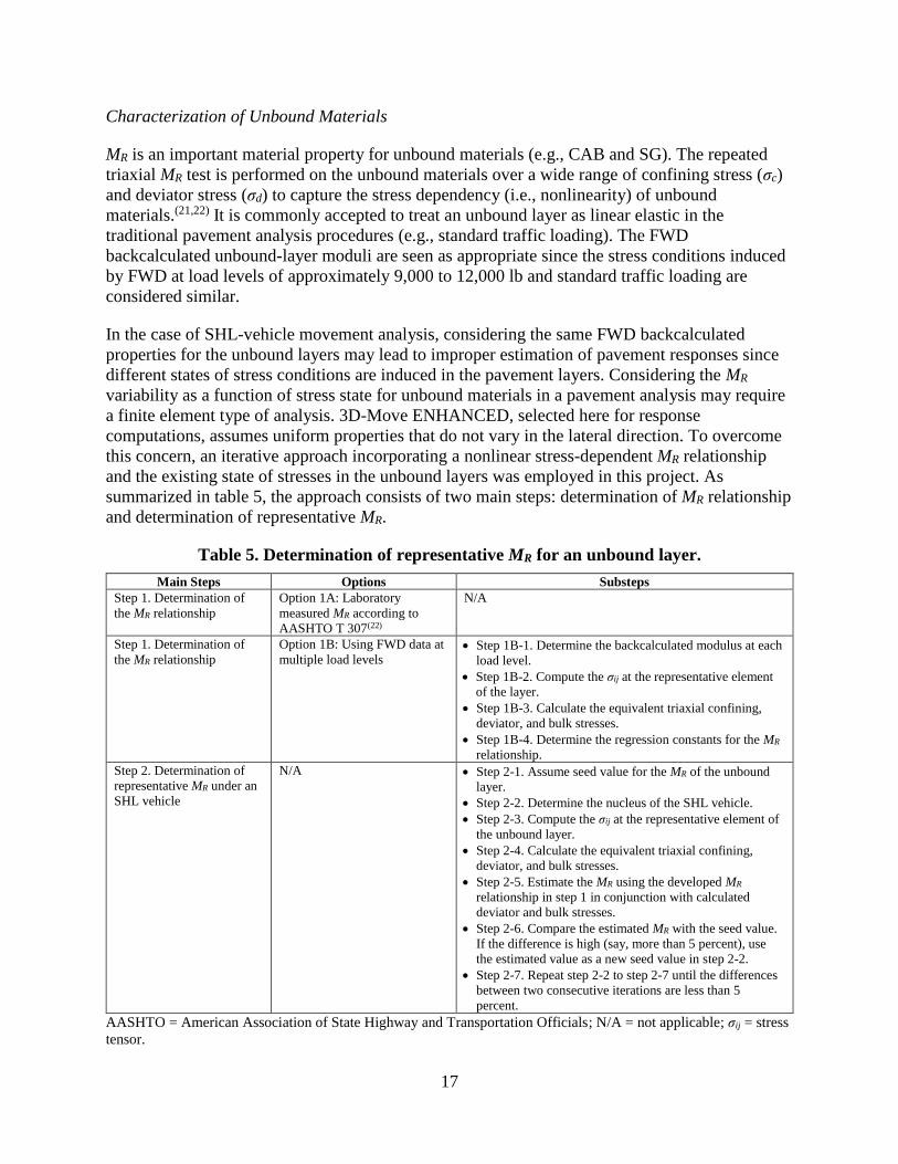
Characterization of Unbound Materials

MR is an important material property for unbound materials (e.g., CAB and SG). The repeated

triaxial MR test is performed on the unbound materials over a wide range of confining stress (σc)

and deviator stress (σd) to capture the stress dependency (i.e., nonlinearity) of unbound

materials.(21,22) It is commonly accepted to treat an unbound layer as linear elastic in the

traditional pavement analysis procedures (e.g., standard traffic loading). The FWD

backcalculated unbound-layer moduli are seen as appropriate since the stress conditions induced

by FWD at load levels of approximately 9,000 to 12,000 lb and standard traffic loading are

considered similar.

In the case of SHL-vehicle movement analysis, considering the same FWD backcalculated

properties for the unbound layers may lead to improper estimation of pavement responses since

different states of stress conditions are induced in the pavement layers. Considering the MR

variability as a function of stress state for unbound materials in a pavement analysis may require

a finite element type of analysis. 3D-Move ENHANCED, selected here for response

computations, assumes uniform properties that do not vary in the lateral direction. To overcome

this concern, an iterative approach incorporating a nonlinear stress-dependent MR relationship

and the existing state of stresses in the unbound layers was employed in this project. As

summarized in table 5, the approach consists of two main steps: determination of MR relationship

and determination of representative MR.

Table 5. Determination of representative MR for an unbound layer.

Main Steps Options Substeps


the MR relationship

Option 1A: Laboratory

measured MR according to

AASHTO T 307(22)

N/A

Step 1. Determination of Option 1B: Using FWD data at • Step 1B-1. Determine the backcalculated modulus at each the MR relationship multiple load levels load level.

• Step 1B-2. Compute the σij at the representative element

of the layer.

• Step 1B-3. Calculate the equivalent triaxial confining,

deviator, and bulk stresses.

• Step 1B-4. Determine the regression constants for the MR

relationship.


representative MR under an

SHL vehicle

N/A • Step 2-1. Assume seed value for the MR of the unbound

layer.

• Step 2-2. Determine the nucleus of the SHL vehicle.

• Step 2-3. Compute the σij at the representative element of

the unbound layer.

• Step 2-4. Calculate the equivalent triaxial confining,

deviator, and bulk stresses.

• Step 2-5. Estimate the MR using the developed MR

relationship in step 1 in conjunction with calculated

deviator and bulk stresses.

• Step 2-6. Compare the estimated MR with the seed value.

If the difference is high (say, more than 5 percent), use

the estimated value as a new seed value in step 2-2.

• Step 2-7. Repeat step 2-2 to step 2-7 until the differences

between two consecutive iterations are less than 5

percent.

AASHTO = American Association of State Highway and Transportation Officials; N/A = not applicable; σij = stress

tensor.

17

e = s1ooof1J

8 = 1200qu

Characterization of Chemically Stabilized Materials

The chemically stabilized materials consist of lean-concrete, cement-stabilized, open-graded-

cement-stabilized, soil-cement, and lime-treated materials. These materials are considered linear

elastic with constant elastic modulus (E), which can be determined from the existing correlations

with compressive strength (f'c). For instance, figure 12 and figure 13 present the equations for

calculating E for lean concrete and cement-treated base (CTB) as well as soil cement.(14) Then

the engineer may apply some reduction factors on the calculated modulus based on the measured

or perceived cracking condition of the stabilized layer. Backcalculation using FWD data can also

help in determining in situ MR values.

Figure 12. Equation. Estimation of E for lean concrete and CTB.

Figure 13. Equation. Estimation of E for soil cement.

Where qU is unconfined f'c (psi).

2.2.2. SG τmax Properties

As mentioned in section 2.2, investigating the likelihood of shear failure (i.e., ultimate and

localized) in the pavement SG subjected to SHL movement requires the τmax properties for the

SG. The τmax parameters ( and c) are not readily available and are not used in routine pavement

design processes. Although existing database or engineering judgment can provide information

regarding the strength properties of the SG layer, many researchers have questioned the validity

of such estimates. In addition, because of the variability of the SG, a realistic estimation under in

situ conditions for the influenced zone in the SG (i.e., pavement SG layer) is more appropriate.

Although laboratory testing provides the most reliable measurements for τmax parameters of

unbound materials (e.g., base and SG), the time-consuming and destructive process of sample

collection, testing, and associated costs is an objectionable limitation. In this study, an FWD-

based procedure was developed for estimating in situ τmax parameters of the SG contained within

the influenced zone (i.e., pavement SG layer) that impact pavement performance. The concept

behind this methodology was to identify an equivalent triaxial condition for the representative

element of the SG layer under FWD loading.(23,24) To this end, the nonlinear stress dependency

of SG materials under multiple FWD-load levels along with the extension of the commonly

accepted hyperbolic stress–strain relationship of unbound materials applied at the lower FWD-(25,26) induced state of stresses were used (figure 14 and figure 15).

In this methodology, the stress tensor (σij) at a representative element in the SG is calculated first

by using a layered linear elastic program (e.g., 3D-Move ENHANCED using static condition)

that simulates each of the applied FWD-load levels.(11) The analysis utilizes the backcalculated

modulus at each of the respective FWD-load levels. Such an approach inherently considers the

role of stress dependency in an unbound material. The calculated σij are transformed to the

equivalent stress conditions associated with triaxial compression tests (d and c) for each of the

18

o9 /

c/J I

,,, --- -

cP Extrapolation

I <f)

Axial Strain, E1

-

Extrapolation

Axial Strain, E1

- - - - -- -O FWD-induced Equivalent

Triaxial Stress-Strain Condition

- Hyperbolic Stress-Strain Relationship

---Deviator Stress at Failure

0 FV.'D-induced Equivalent Triaxial Stress-Strain Condition

- L inear Fonn ofHype1t >0lic Stt·essStrnin l<el aticmship

FWD-load levels using the stress invariants (i.e., octahedral stress components). A hyperbolic

relationship (figure 16) is subsequently fitted to the equivalent triaxial test datasets of d and

axial strain (1). By rewriting the hyperbolic equation in a linear form in terms of ε1/σd and ε1

(figure 17), σd at failure (df) and initial tangent modulus (Ei) can be estimated by inversing the

slope and intercept, respectively. Volume V: Appendix D describes in greater detail the FWD-

based procedure as well as the verification exercises.(4) The Mohr–Coulomb failure envelope

equation is subsequently used in the estimation of the SG c by assuming an acceptable range for

the .

© 2018 UNR.

Figure 14. Graph. Extrapolation of hyperbolic relationship.

© 2018 UNR.

Figure 15. Graph. Estimation of df using linear form of hyperbolic relationship.

19

qu = cNc Fcs Fed Fd + q' Nq Fqs Fqd Fqi + 2 y B Ny Fys Fyd Fyi

Figure 16. Equation. Nonlinear hyperbolic stress–strain relationship of soils.

Figure 17. Equation. Hyperbolic relationship in linear form.

2.3. ULTIMATE FAILURE ANALYSES

Ultimate failure analyses include the investigation of the SG bearing failure as well as sloped-

shoulder failure. In this section, these two analyses are briefly explained. Volume VI: Appendix

E and Volume VII: Appendix F provide detailed discussion regarding these analyses.(5,6)

2.3.1. SG Bearing Failure Analysis

SHL vehicles with nonconventional axle and tire loadings and configurations can render a

critical condition of shear failure either in an ultimate or localized manner. Ultimate shear failure

is an instantaneous failure and focuses on the SG layer as it is typically the weakest layer in the

pavement structure.

To examine the risk of instantaneous shear failure, Meyerhof’s general bearing capacity equation

(figure 18) is viewed as an ideal selection because it is a well-established and validated

foundation design analysis procedure under static or slow-moving vehicle loading conditions.(27)

Accordingly, the distributed σv induced by the SHL vehicle on top of the influenced SG layer is

compared with the bearing capacity of the layer to identify the possibility of ultimate shear

failure in the pavement SG layer. It should be noted that a modified bearing capacity equation is

applied when a sloping pavement shoulder is present.(27)

Figure 18. Equation. Meyerhof’s general bearing capacity.

Where:

q' = effective stress at the bottom of the foundation level.

γ = unit weight of SG soil.

B = width of the foundation (or diameter).

Fcs = shape factor with respect to c.

Fqs = shape factor with respect to overburden.

Fγs = shape factor with respect to unit weight.

Fcd = depth factor with respect to c.

Fqd = depth factor with respect to overburden.

Fγd = depth factor with respect to unit weight.

Fci = load inclination factor with respect to c.

20

14 ■ 12-14 '1 12 '-' ;,,; 10-12 ~ 10 ~ -en 8 ::: 8-10

:z 6-8 ~ 6

:-= 4-6 '-' 4 :p :i:l 2 >

0 ~ 2-4

:se 0-2

Fqi = load inclination factor with respect to overburden.

Fγi = load inclination factor unit weight.

Nc = bearing capacity factor with respect to cohesion.

Nq = bearing capacity factor with respect to overburden.

Nγ = bearing capacity factor with respect to unit weight.

As mentioned in section 2.1.2, the SHL vehicle may consist of several individual axle groups,

and each axle group has a nucleus (figure 10). To identify the possibility of ultimate shear failure

in the pavement SG layer, each axle group is individually assumed to be a bearing capacity

investigation zone (i.e., loaded area). Accordingly, the distributed σv on the top of the SG

induced by the nucleus of an axle group is compared against the bearing capacity of the SG

layer. It should be noted that the dimension of the bearing capacity investigation zone in

Meyerhof’s equation is specified as being equal to the length and width of the axle group.

It is expected that the nucleus-induced σv on top of the SG represents a nonuniform distribution.

As an example, computed σv distribution for the nucleus of SHL case No. LA-8T-14 (figure 10)

is depicted in figure 19. However, Meyerhof’s equation assumes the loaded area to be of a

certain fixed shape with a uniform pressure distribution. The average uniform σv (qave) induced

by the nucleus can be calculated by first integrating the volume of the nucleus-induced σv

distribution on top of the SG and then dividing it by the area of the uniform stress distribution

induced by the nucleus on top of the SG (Aaffected), as illustrated in figure 20.

© 2018 UNR.

Figure 19. Chart. σv distribution on top of the SG under the nucleus (case No. LA-8T-14).

21

ffected

■ 12-14

;,,; 10-12

::: 8-10

~ 6-8

:-= 4-6

~ 2-4

:se 0-2

© 2018 UNR.

Figure 20. Chart. σv distribution on top of the SG under the nucleus and Aaffected (case No.

LA-8T-14).

As a conservative measure, qave is assumed to cover the entire rectangular area of the axle group.

This stress distribution can be considered the most critical possible scenario. It may be noted that

a smaller subset of tires or axles within the SHL truck may be assumed to be the bearing capacity

investigation zone (i.e., loaded area). However, it is physically impossible, because of the

interconnectivity of the axles, to have one part of the vehicle develop a general bearing capacity

failure mechanism while the rest does not. The entire axle group, since it is interconnected, will

behave as a unit, and therefore, the failure should be undertaken for the entire axle group.

2.3.2. Sloped-Shoulder Failure Analysis

Although slope stability is one of the common problems in geotechnical practice, it has not been

a major concern for a pavement shoulder subjected to the standard truck loading. However,

substantial higher surcharge load resulting from the SHL movements might lead to a critical

condition for failure.

SHL vehicles are usually moved under traffic control, so it is often possible to keep the SHL

vehicle far away from the pavement edge and shoulder. It is recommended that the vehicle stay

away from the pavement edge, particularly in routes where there is an unpaved shoulder and/or a

steep slope. However, it is not always possible to keep the SHL vehicle far from the pavement

edge (e.g., narrow lanes and/or a wide SHL vehicle). Therefore, it is necessary to investigate the

stability of a sloped pavement shoulder under the SHL-vehicle movement.

The wedge method is a well-accepted slope stability–analysis methodology in geotechnical

practice.(28) In this research study, wedge-method slope stability analysis was modified so that

stability of a sloping layered medium consisting of pavement layers with distinct properties

could be evaluated under SHL movements. The following briefly presents the modified slope

stability wedge method; details are presented in Volume VII: Appendix F.(6)

22

AC Layer CAB Layer

Travel Direction

I Edgeof / I Travel Lane SHL Loading

II D00 0 000CODOO O O ~ OOD O DCDDOOOD C O D O D C O D DDDD D D C O

AC Layer

CAB Layer

SG Layer

Horizontal Boundaries of Wedges

Figure 21 illustrates a typical flexible pavement structure with a sloped shoulder. As illustrated

in this figure, to investigate the stability of a pavement shoulder subjected to SHL movement,

various wedges of failure are selected. This figure shows several slip surfaces passing through

point A as solid lines. In all cases, the failure wedge is bounded by a vertical plane, and a

horizontal or an inclined slip surface is located in the SG layer. The vertical plane is located to

the left of the AC layer as it is assumed that the vertical plane cannot extend through the AC

layer. It is also assumed that the slip surface is developed in the SG layer, which is the weakest

layer in the pavement structure. Searching for the critical location of the failure wedge involves

systematically varying the horizontal boundaries of the wedges until the corresponding minimum

factor of safety (FOS) is found.

© 2018 UNR.

Figure 21. Illustration. Search schemes for failure wedges.

The stability of each failure wedge is evaluated by considering the wedge as a rigid sliding mass

or a gravity-retaining structure. As shown in figure 22 and figure 23, the following five forces

acting on the failure wedge can be identified:

• Weight of the sliding wedge (W).

• Developed resisting c force resulting from the mobilized c (TD) acting on the bottom slip

surface.

• Resultant force from the bottom soil (FD) that makes an angle (ϕD) with the normal to the

bottom slip surface.

• Two components of horizontal deriving forces acting on the vertical plane: lateral earth

pressure from adjacent soil (Q) and resultant horizontal force due to surcharge load (P)

(i.e., SHL vehicle).

23

CAB Layer

Q+P

SG Layer

To

(Wcose - (Q + P)sin0wedge)tanc/) + c ,. l FOS = ·

(Wsin0wed,qe + (Q + P)cos0wed,qe)

Wtancp + c * l FOS = p + Q

© 2018 UNR.

Figure 22. Illustration. Failure wedge with horizontal slip surface and applied forces.

© 2018 UNR.

Figure 23. Illustration. Failure wedge with inclined slip surface and applied forces.

To determine the FOS, the force equilibrium equations in the parallel and perpendicular

directions to the slip surface are applied. Consequently, the FOS using the equations presented in

figure 24 or figure 25 can be determined. Here, wedge is the angle between the slip surface and

horizontal surface (figure 23), and l is the length of the bottom slip surface. For the failure

wedges with horizontal slip surface where wedge is 0, the FOS can be simplified to the equation

shown in figure 25.

Figure 24. Equation. FOS against failure for the wedges with inclined slip surface.

Figure 25. Equation. FOS against failure for the wedges with horizontal slip surface.

Q is calculated using the Rankine active earth pressure, which is a well-accepted theory in the

design of retaining structures. To estimate the resultant horizontal force due to a surcharge SHL

vehicle (P), 3D-Move ENHANCED is utilized so that the role of layered pavement structure

with distinctly different material properties is considered.(11)

24

Subsequently, 3D-Move ENHANCED computed horizontal stresses are modified through the

application of a stress adjustment factor for sloping shoulder (SAFShoulder) to account for the role

of a sloping shoulder near the edge of the pavement since this software assumes that pavement

layers extend laterally to infinity. SAFShoulder equal to 1.5 was determined based on the results

obtained from the large-scale experiments conducted.(23) Discussion regarding the determination

of SAFShoulder is presented in chapter 3.

A similar exercise is followed in geotechnical practice when the value of P is calculated based on

the Boussinesq theory assuming elastic, homogenous, and isotropic semi-infinite soil

medium.(27,28) Subsequently, the calculated horizontal stress using the Boussinesq solution is

doubled to account for the yielding soil continuum (i.e., SAFShoulder equal to 2).

2.4. BURIED UTILITY RISK ANALYSIS

As part of this project, a study was carried out to assess the risk against failure in existing buried

utilities due to SHL movement, which is described in Volume VIII: Appendix G.(7) Review of

the existing state-of-practice methods that are employed for the design of buried utilities revealed

that every utility has certain specific design considerations that are unique to that particular

buried utility. However, two common steps of design are followed by all methods. In the first

step, the focus is on the determination of load distribution on the buried utility structure due to

the dead (i.e., soil overburden) and live (i.e., standard truck traffic) loads. Once the load

distribution is obtained, the structural design is then dictated by specifications for the buried

utility type.

Procedures to analyze the risk of failure in flexible and rigid buried structures due to SHL

movement were developed in a similar fashion in this study. Reliable assessment of induced

stresses due to live load (i.e., SHL-vehicle load) and subsequent investigation of buried utility

integrity subjected to the induced stresses are the main components of the developed procedures.

Widely accepted and available buried utility design procedures were adopted in this study to

assess the failure risk of existing buried utilities under SHL vehicle–induced stresses.

For flexible pipes, a hybrid step-by-step evaluation procedure provided in American Lifelines

Alliance (ALA) and Canadian Energy Pipeline Association (CEPA) reports was implemented in

this study.(29,30) The procedure is divided into four general checks:

1. Assess FOS against pipe circumferential stress failure.

2. Check ovality of pipe cross section.

3. Check ring buckling stress.

4. Check wall crushing stress.

In the case of rigid concrete culvert, the stability of a rigid buried utility is investigated by

analyzing the flexural strength, τmax , and axial thrust in the culvert members (i.e., top slab,

bottom slab, and sidewalls) in accordance with AASHTO [American Association of Highway and

Transportation Officials] LRFD [Load and Resistance Factor Design] Bridge Design

Specifications.(31)

25

SHL Vehicle

3D-Move ENHANCED computed load- SG induced stresses

Although the state of practice provides recommendations with respect to the live load

distribution, their application is questionable for assessing the risk of buried utilities under an

SHL-vehicle movement. Consideration of only a standard truck (mostly HS20) as a live load and

simulating it as a point or rectangular load that is statically applied at the surface of unpaved

roads (i.e., neglecting the AC and CAB layer) are the significant limitations for the application to

SHL-vehicle movement. Therefore, adoption of 3D-Move ENHANCED was seen as more

appropriate because of its merits to realistically simulate pavement structure and SHL vehicles.

Accordingly, the load-induced σv at the location of buried utility is computed using 3D-Move

ENHANCED (zz-3D-Move) (figure 26).(11) The role of soil–structure interaction and discontinuities

within the medium (i.e., existence of buried utilities) is accounted for by using a stress

adjustment factor for buried utilities (SAFUtility). Therefore, computed σv using 3D-Move

ENHANCED at the location of the buried utility were modified and utilized in the analysis.(11)

© 2018 UNR.

Figure 26. Illustration. Computation of σv at the location of buried utility using 3D-Move (11) ENHANCED.

The behavior of buried utilities observed in the large-scale experiments conducted were

employed to determine SAFUtility for flexible steel pipe and rigid concrete box culvert. It was

found that the σv experienced by the flexible pipe were much lower than those stresses

transferred in the continuum medium (i.e., no buried utility). In the case of concrete culvert,

substantially higher σv were measured on top of concrete culvert when compared with those

induced in the soil medium under the control condition (i.e., no buried utility). As a conservative

measure, it is recommended to retain SAFUtility for flexible pipes as 1. This recommendation is

mainly to be on the conservative side until further experimental testing and numerical

investigations are carried out. However, in the case of rigid culverts, SAFUtility equal to 1.5 is

recommended.

26

Mohr-Coulomb

2.5. SERVICE LIMIT ANALYSES

The service limit analyses include localized shear failure analysis and deflection-based service

limit analysis. The localized shear failure analysis investigates the likelihood of localized failure

(yield) at the critical location on top of the SG layer under the SHL vehicle. The deflection-based

service limit analysis assesses the magnitude of the load-induced pavement deflections during

the SHL movement. The following sections describe these procedures; detailed discussions are

presented in Volume Ⅵ: Appendix E.(5)

2.5.1. Localized Shear Failure Analysis

As mentioned in section 2.2, ultimate failure analysis (SG bearing failure and, when applicable,

sloped-shoulder failure) is an essential first step for evaluating the risk of shear failure in the

pavement SG subjected to SHL movement. Once this analysis confirms the bearing capacity of

the SG is adequate, the likelihood for onset of yielding in the SG layer due to localized shear

failure is then examined. It is believed that the substantial SHL vehicle–induced state of stress

developed in the pavement structure might reach close to the failure state. Therefore, comparing

the load-induced stress level on top of the SG layer with the corresponding yield criterion for this

layer is carried out in localized shear failure analysis. It may be noted that the localized shear

failure analysis focuses on the SG layer, which typically represents the most vulnerable

pavement layer with the lowest strength.

Several failure criteria, such as Mohr–Coulomb, Drucker–Prager, Lade–Duncan, and Matsuoka– Nakai, have been proposed for evaluating the yielding (i.e., failure) of soil materials.(28) The

Drucker–Prager yield criterion that involves the τmax parameters (ϕ and c) of material is one of

the well-accepted criteria in soil plasticity.(32) As presented in figure 27, the Drucker–Prager

yield criterion includes the Mohr–Coulomb criterion for 3D stress states.

Per Drucker and Prager, σd is represented as q. The Drucker–Prager failure criterion is a straight

line on a q versus mean normal stress (p) plot. Figure 28 demonstrates the Drucker–Prager

failure envelope in q–p space. As presented in this figure, at a certain induced mean normal

stress (papplied), the FOS is defined as the ratio between the Drucker and Prager’s deviator stress

at failure (qfailure) and induced deviator stress (qapplied). FOS is an indication of how far the stress

state is from the failure envelope.

© 2018 UNR.

Figure 27. Illustration. The Drucker–Prager and Mohr–Coulomb yield surfaces.

27

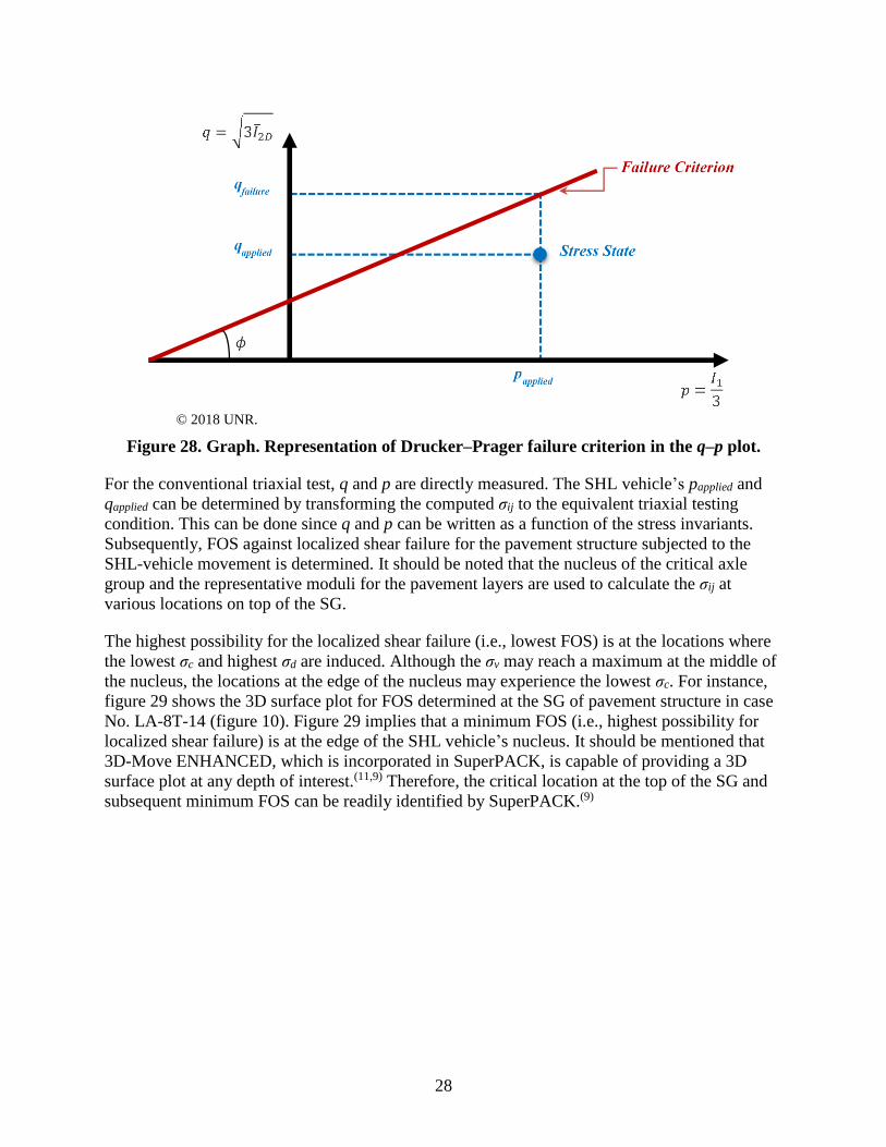
qapplietl Stress State

Papplietl

© 2018 UNR.

Figure 28. Graph. Representation of Drucker–Prager failure criterion in the q–p plot.

For the conventional triaxial test, q and p are directly measured. The SHL vehicle’s papplied and

qapplied can be determined by transforming the computed σij to the equivalent triaxial testing

condition. This can be done since q and p can be written as a function of the stress invariants.

Subsequently, FOS against localized shear failure for the pavement structure subjected to the

SHL-vehicle movement is determined. It should be noted that the nucleus of the critical axle

group and the representative moduli for the pavement layers are used to calculate the σij at

various locations on top of the SG.

The highest possibility for the localized shear failure (i.e., lowest FOS) is at the locations where

the lowest σc and highest σd are induced. Although the σv may reach a maximum at the middle of

the nucleus, the locations at the edge of the nucleus may experience the lowest σc. For instance,

figure 29 shows the 3D surface plot for FOS determined at the SG of pavement structure in case

No. LA-8T-14 (figure 10). Figure 29 implies that a minimum FOS (i.e., highest possibility for

localized shear failure) is at the edge of the SHL vehicle’s nucleus. It should be mentioned that

3D-Move ENHANCED, which is incorporated in SuperPACK, is capable of providing a 3D

surface plot at any depth of interest.(11,9) Therefore, the critical location at the top of the SG and

subsequent minimum FOS can be readily identified by SuperPACK.(9)

28

11 10

9 8 7 6 5 4 3 2 1 0

FOS(minimum) = 1.1

:::: 0-1 2i1 1-2 ~ 2-3 ~ 3-4 :?~ 4-5 ~ 5-6 @6-7 ilill 7-8 11 8-9 ■ 9-10 ■ 10-11 ■ 11-12

12

© 2018 UNR.

Figure 29. Chart. FOS under SHL-vehicle nucleus.

2.5.2. Deflection-Based Service Limit Analysis

Although the shear failure analyses (i.e., ultimate and localized) may inform that the pavement

structure is capable to sustain the SHL movement without experiencing any shear failure, the

pavement structure could still be subjected to excessive surface deflection under an SHL vehicle

that may eventually lead to the development of premature surface distresses and rapid

deterioration. To prevent this, the SHL vehicle–induced surface deflection (δSHL) should be

determined and limited to an allowable surface displacement. It may be noted that the nucleus of

the critical axle group and the representative moduli for the pavement layers are used to compute

δSHL.

In the deflection-based service limit analysis, an equivalent FWD-load level (FWDequiv), which

generates surface center deflection at the center of the FWD plate (D0) equal to δSHL, is

determined. In other words, the equivalency is established between the SHL-vehicle load and an

FWD-load level (i.e., FWDequiv) based on the same induced surface deflection. Subsequently,

FWDequiv is compared to an allowable FWD-load level (FWDallow). An FWDequiv higher than

FWDallow indicates a need for mitigation strategies.

To determine the FWDequiv, the FWD load–deflection curve is developed using the load and D0

measurements at multiple FWD-load levels (figure 30). However, the AC-layer temperature at

the time of SHL movement, referred to as analysis temperature, may be different from the time

of FWD testing. Therefore, measured D0 needs to be adjusted based on the analysis temperature.

To accomplish this, the AC-layer stiffness at the analysis temperature is determined using the

field damaged E* master curve and knowing the FWD-loading frequency. Accordingly, surface

deflections at different FWD-load levels are calculated using the determined AC-layer stiffness

(i.e., temperature adjusted) and along with backcalculated resilient moduli of the unbound layers

29

,-... 'B 0.08 .s '-' = 0.07 Cl,

s ci, 0.06 <.I

!!I -~ 0.05 A ~ 0.04 ,!: ... &J 0.03

-~ .l,c 0.02 .... ... Cl,

> 0.01

0

0 5,000

FWD load-deflection curve

10,000 15,000 20 ,000 25 ,000 30,000

Applied FWD Load (lb)

at the corresponding FWD load, using the static loading condition in 3D-Move ENHANCED.(11)

Consequently, knowing the calculated δSHL and developed FWD load–deflection curve, the

FWDequiv to the SHL-vehicle load is identified as illustrated in figure 30.

© 2018 UNR.

Figure 30. Chart. FWD load–deflection curve.

The concept of shear stress ratio (SSR) was employed to determine the FWDallow. Previous

studies reported that permanent deformation potential of unbound materials (i.e., CAB and SG)

could be reasonably assessed by means of the SSR concept.(33–36) As illustrated in figure 31, the

SSR is defined as the ratio between applied (mobilized) shear stress (τmobilized) and the material’s

τmax. It has been concluded that when unbound materials experience SSR values higher than 0.7,

high permanent strain accumulates in the materials, eventually resulting in permanent

deformation.(33–36) Accordingly, the FWD-load level that induces an SSR value equal to 0.7 in

the pavement SG layer (top of SG) is identified as FWDallow.

The AC-layer stiffness at the analysis temperature predetermined using field damaged E* master

curve along with the backcalculated resilient moduli of the unbound layers at multiple FWD-load

levels are employed to calculate the σij. Here, the point of interest is located below the center of

the simulated FWD-loading plate on top of the SG. Subsequently, σij is transformed into

equivalent σc and σd in laboratory triaxial testing conditions by the use of stress invariants.

Knowing the FWD-induced σd and σc, the FWD load–SSR curve representing the SSR values at

multiple FWD-load levels is established. As illustrated in figure 32, this can be used to obtain the

FWDallow corresponding to an SSR value equal to 0.7.

30

'l' Mohr-Coulomb Failure Envelope ------ -., ' ' ' ,,

'l',nnx --------------------------------------

~

C

1

0.9

0.8

0.7

0.6

~ 0.5

0.4

0.3

0.2

0.1

0 0 5,000

q c <Tmobilized

t ----• .... -::-. ~ ,, ~ FWD Load-SS

, ~ Relationship ,, ., F\VDa11ow

10 ,000 15 ,000 20,000 25 ,000

Applied FWD Load (lb)

(1

30,000

© 2018 UNR.

Figure 31. Chart. Representation of τmax and applied stresses.

© 2018 UNR.

Figure 32. Chart. FWD load–SSR curve.

2.6. COST ALLOCATION ANALYSIS

SHAs issue special permits for SHL-vehicle movements and collect a nominal fee, making SHL-

vehicle operation legal on their highway network. However, quantifying pavement damage

attributed to an SHL movement is a challenging task. An array of factors specific to each SHL

movement (e.g., axle and tire loadings and configurations, traveling speed, and temperature and

properties of existing pavement layers at the time of the movement) influences the magnitude of

the load-induced pavement damage.

SHL vehicles generally present a nonstandard axle configuration, and any additional pavement

damage caused by their operation is generally not considered in the new and rehabilitation

31

designs of pavements. Since heavier axle loads of SHL vehicles can introduce greater stresses

and strains in the pavement compared to those estimated under a traditional truck loading, a

single SHL-vehicle pass could induce damage similar to that caused by multiple passes of a

standard truck, leading to a faster deterioration rate in the pavement condition.

Another challenge associated with determining pavement damage attributable to an SHL

movement is properly accounting for the characteristics of the existing pavement layers at the

time of the movement. For instance, the viscoelastic property of the AC layer is critical as it

influences the load-induced pavement responses with the SHL movements often being at much

lower speeds. For example, pavement damage caused by an SHL vehicle operating during the

summer (or even daytime hours) may be significantly different from the damage caused by the

same vehicle operating during a different season (or during nighttime hours of the same day).

One of the objectives in this research project was to establish an appropriate mechanistic-based

cost allocation methodology for SHL movement on flexible pavements. The procedure

developed in this study allows for the estimation of PDACs due to a single pass of an SHL

vehicle. The PDAC can be estimated for different SHL-vehicle axle loadings and configurations

with due considerations given to locally calibrated pavement distress models, existing pavement

condition, different pavement repair options, and vehicle miles traveled (VMT).

The approach suggested by Tirado et al. of using the highway cost-occasioned method to

estimate PDACs based on ME analysis was adopted in this project.(37) This cost allocation

approach estimates pavement-damage costs considering the predicted pavement life reduction

due to a single pass of the SHL vehicle. With this method, different pavement distress models,

pavement repair options, and any axle configuration can be implemented. The net present value

(NPV) of repair costs and VMT are also needed inputs of the process.

The approach presented by Tirado et al. was revised, in this study, to consider the condition of

the pavement at the time of the SHL-vehicle movement. Consequently, lower PDACs have been

estimated when an SHL movement occurs on a pavement section with lower remaining life (i.e.,

a pavement section that has already been subjected to a large percentage of its original design

truck traffic).

To estimate PDAC, distress prediction models are needed to predict pavement performance and

estimate pavement damage under both SHL vehicles and reference vehicles. The estimated

damage is then used to calculate the PDAC due to a single pass of the SHL vehicle. The overall

flowchart for the cost allocation analysis method is presented in figure 33. It should be noted that

the damage caused by a single pass of the SHL vehicle is compared to that of a reference vehicle.

The equivalency concept is used in the determination of cost attributable to SHL-vehicle

movement.

There are cases when the SHL-vehicle configuration has several trailers, or dollies, comprising

multiple tires and complex and specialized axle arrangements. This type of configuration

requires the determination of the nucleus so that the SHL vehicle is divided into one or more

numbers of nuclei where the nucleus repeats itself across the SHL-vehicle configuration;

therefore, the number of nucleus repetitions within the SHL truck domain is considered for

pavement damage costs calculation instead of individual axle repetitions. It should be noted that

32

this approach is consistent with the pavement response analysis and estimation of pavement

damage using MEPDG methodology for different axle types (i.e., single, tandem, tridem, and

quad axles).(14) In cases when the spacing between two trailers is greater than 60 inches, they are

treated as independent groups by defining a separate nucleus for each group.

Distress and Prediction

Model Selection

Reference

Vehicle

SHL Analysis

Vehicle

Generate Damage Curves Generate Damage Curves

Calculate Number of

Vehicle Passes to

Failure Nstd:f

Calculate Amount of

Distress After a Given

Number of Passes,

dSTD

Calculate Number of

Vehicle Passes to

Cause Same Distress

as dSTD

Calculate Distress

Corresponding to

One Extra Pass of

SHL Analysis Vehicle

Calculate the Equivalent

Number of Reference Vehicle

Passes to Cause Same Distress

as One Pass of SHL Analysis

Vehicle

Calculate Percent of

Pavement Life

Reduction Due to

One Pass of SHL

Analysis Vehicle, LR

Years to Reach

Failure

Selected Pavement

Repair Option

Pavement Repair

Costs, $/Lane Mile

Present Worth Value

of Repair, PWV

Pavement Damage

Associated Costs

PDAC = PWV x LR x RSL

Remaining Service Life of

Pavement: RSL, %

Modified from © 2010 Tirado et al. Reprinted by permission from SAGE Publications, Inc.

Figure 33. Flowchart. Overall approach for the estimation of pavement damage and

allocated cost.(37)

33

2.7. MITIGATION STRATEGIES

The analysis procedures for evaluating SHL movement on flexible pavements that are developed

in this study consisted of the following four major components: ultimate failure analyses, buried

utility risk analysis, service limit analyses, and cost allocation analysis.

Prior to the conducting of cost allocation analysis and determination of PDAC, ultimate failure

analyses, buried utility risk analysis, and service limit analyses need to be completed to assess

the potential impact of SHL movement on flexible pavements. It should be noted that mitigation

strategies may be needed at any stage of the evaluation process when the calculated results fail to

meet the imposed respective requirements.

Table 6 presents mitigation strategies that can attenuate the SHL vehicle–induced distresses and

damages, whereas some of the strategies are limited to only one type of distress (or failure). It is

also noted that 3D-Move ENHANCED, which is the analysis engine of SuperPACK, is capable

of modeling the layer interface conditions, such as debonding or slippage.(11,9) Therefore,

simulation of debonded layers or mat (e.g., steel plate, aggregate base cover) can be conducted

whenever the analyses procedures indicate the need for application of mitigation strategies.

These remedial strategies should be considered on an individual basis using SuperPACK.(9)

Table 6. Select mitigation strategies applicable to SHL movement.

Mitigation Strategy Advantages Additional Considerations

Surface protection and load

dispersion: Deploy steel plate. • • •

Spreads the load over a larger area.

Easy to deploy.

Applicable for ultimate failure, buried

utility failure, and service limit failure.

•

•

Cost (e.g., heavy hauling

equipment and

supervision).

Safety.


dispersion: Deploy timber

mat.

• • •


Easy to deploy.



• Efficiency (e.g., labor

intensive).


dispersion: Deploy concrete

slab.

• •




•

•

Cost (e.g., design,

materials, and placement).

Time consuming.


dispersion: Provide aggregate

base cover.

• •




•

•

Cost (e.g., relatively lower

cost for design, materials,

and placement).

Time consuming.

Increase the clearance from

the sloped edge. • Easy to apply. • Applicable only for sloped-

shoulder failure.

Reduce the operating pressure

in the pipe. • Easy to apply. • Applicable only for

flexible buried utility

failure.

Reassemble SHL-vehicle

configuration. • Applicable for ultimate failure, buried


• •

Cost.

Constraints related to axle

spacing and capacity.

Reroute. • Applicable for ultimate failure, buried


• •

Traffic control.

Longer hauling distances.

34

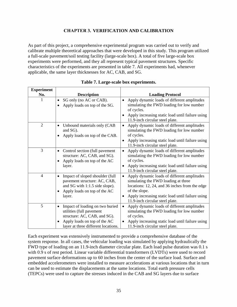
CHAPTER 3. VERIFICATION AND CALIBRATION

As part of this project, a comprehensive experimental program was carried out to verify and

calibrate multiple theoretical approaches that were developed in this study. This program utilized

a full-scale pavement/soil testing facility (large-scale box). A total of five large-scale box

experiments were performed, and they all represent typical pavement structures. Specific

characteristics of the experiments are presented in table 7. All experiments had, whenever

applicable, the same layer thicknesses for AC, CAB, and SG.

Table 7. Large-scale box experiments.

Experiment

No. Description Loading Protocol

1 • SG only (no AC or CAB).

• Apply loads on top of the SG.

• Apply dynamic loads of different amplitudes

simulating the FWD loading for low number

of cycles.

• Apply increasing static load until failure using

11.9-inch circular steel plate.

2 • Unbound materials only (CAB

and SG).

• Apply loads on top of the CAB.



of cycles.



3 • Control section (full pavement

structure: AC, CAB, and SG).

• Apply loads on top of the AC

layer.



of cycles.



4 • Impact of sloped shoulder (full

pavement structure: AC, CAB,

and SG with 1:1.5 side slope).


layer.


simulating the FWD loading at three

locations: 12, 24, and 36 inches from the edge

of the slope.



5 • Impact of loading on two buried

utilities (full pavement

structure: AC, CAB, and SG).


layer at three different locations.



of cycles.



Each experiment was extensively instrumented to provide a comprehensive database of the

system response. In all cases, the vehicular loading was simulated by applying hydraulically the

FWD type of loading on an 11.9-inch diameter circular plate. Each load pulse duration was 0.1 s

with 0.9 s of rest period. Linear variable differential transformers (LVDTs) were used to record

pavement surface deformations up to 60 inches from the center of the surface load. Surface and

embedded accelerometers were installed to measure accelerations at various locations that in turn

can be used to estimate the displacements at the same locations. Total earth pressure cells

(TEPCs) were used to capture the stresses induced in the CAB and SG layers due to surface

35

loading. Strain gauges were attached to the AC layer as well as the utility pipe to provide the

strain distribution resulting from the surface loading.

At different stages of the verification and calibration process, as needed, numerical modeling

using 3D-Move ENHANCED, ILLI-PAVE, and BAKFAA software was employed.(11,38,39) In

addition, FWD measurements as well as laboratory material testing were obtained from the

National Airport Pavement Test Facility (NAPTF) of the Federal Aviation Administration and

from the APT at the University of Costa Rica (UCR), known as LanammeUCR. In this chapter,

brief descriptions of the large-scale box experiments, recorded measurements, and observations

are presented first, followed by details on the verification and calibration exercises.

3.1. LARGE-SCALE BOX DESCRIPTION

The experimental program of this project required a large container to achieve the program’s

objectives. Thus, the research team designed, fabricated, and built a large-scale box with internal

dimensions of 124 by 124 by 72 inches. Figure 34 shows the drawing of the large-scale box. The

large-scale box consisted of a steel base plate, vertical H-shaped steel columns infilled with 4- by

6-inch wood beams and braced at two levels with steel beams and tension rods to act as a lateral

bracing system.

The steel base plate was grouted to the laboratory floor, followed by 20 steel columns

appropriately aligned and welded to the base plate. After the assembly of the steel columns, a

total of 224 wood beams of 4 by 6 by 120 inches were fitted between the columns. Polyvinyl

chloride foam boards were used as filler between the gap inside the web of the columns and the

wood beams. A screw/nut fastening method was used to install the bracing system that consisted

of eight steel beams and four tension rods.

The experimental setup, characterization of material used in the experiments, construction

practice, and instrumentation plans for each experiment are explained in detail in Volume Ⅱ:

Appendix A.(1)

36

© 2018 UNR.

Note: All dimensions are in inches.

Figure 34. Illustration. 3D schematic of large-scale box.

3.2. VERIFICATION AND CALIBRATION EXERCISE

As presented in table 8, multiple theoretical procedures developed in this study were verified or

calibrated using experimental testing and numerical modeling. The processes associated with the

verification and calibration exercises are described in this section.

37

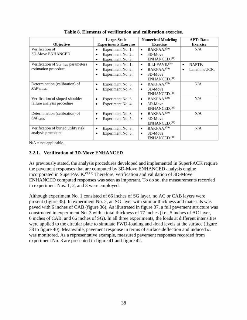
Table 8. Elements of verification and calibration exercise.

Objective

Large-Scale

Experiments Exercise

Numerical Modeling

Exercise

APTs Data

Exercise

Verification of

3D-Move ENHANCED • Experiment No. 1.

• Experiment No. 2.


• BAKFAA.(39)

• 3D-Move

ENHANCED.(11)

N/A

Verification of SG τmax parameters

estimation procedure • Experiment No. 1.



• ILLI-PAVE.(38)

• BAKFAA.(39)

• 3D-Move

ENHANCED.(11)

• •

NAPTF.

LanammeUCR.

Determination (calibration) of

SAFShoulder



• BAKFAA.(39)

• 3D-Move

ENHANCED.(11)

N/A

Verification of sloped-shoulder

failure analysis procedure • Experiment No. 3.


• BAKFAA.(39)

• 3D-Move

ENHANCED.(11)

N/A

Determination (calibration) of

SAFUtility



• BAKFAA.(39)

• 3D-Move

ENHANCED.(11)

N/A

Verification of buried utility risk

analysis procedure • Experiment No. 3.


• BAKFAA.(39)

• 3D-Move

ENHANCED.(11)

N/A

N/A = not applicable.

3.2.1. Verification of 3D-Move ENHANCED

As previously stated, the analysis procedures developed and implemented in SuperPACK require

the pavement responses that are computed by 3D-Move ENHANCED analysis engine

incorporated in SuperPACK.(9,11) Therefore, verification and validation of 3D-Move

ENHANCED computed responses was seen as important. To do so, the measurements recorded

in experiment Nos. 1, 2, and 3 were employed.

Although experiment No. 1 consisted of 66 inches of SG layer, no AC or CAB layers were

present (figure 35). In experiment No. 2, an SG layer with similar thickness and materials was

paved with 6 inches of CAB (figure 36). As illustrated in figure 37, a full pavement structure was

constructed in experiment No. 3 with a total thickness of 77 inches (i.e., 5 inches of AC layer,

6 inches of CAB, and 66 inches of SG). In all three experiments, the loads at different intensities

were applied to the circular plate to simulate FWD-loading and -load levels at the surface (figure

38 to figure 40). Meanwhile, pavement response in terms of surface deflection and induced σv

was monitored. As a representative example, measured pavement responses recorded from

experiment No. 3 are presented in figure 41 and figure 42.

38

1

2

2

~ ~12 ~11 ~10 ~9 ~A7f!j f6

I ~ P4 £'3 f 2 A1A2A3 A4 e,

A1A2A3 A12 A11 A10 A9 ASAffio P9 Ptl

P1

5 A6

SG

1

2

1

2

© 2018 UNR.

All dimensions are in inches; L = LVDT; P = total earth pressure cell; A = accelerometer;

S = strain gauge.

Figure 35. Illustration. Large-scale box experiment No. 1.

© 2018 UNR.


S = strain gauge.


39

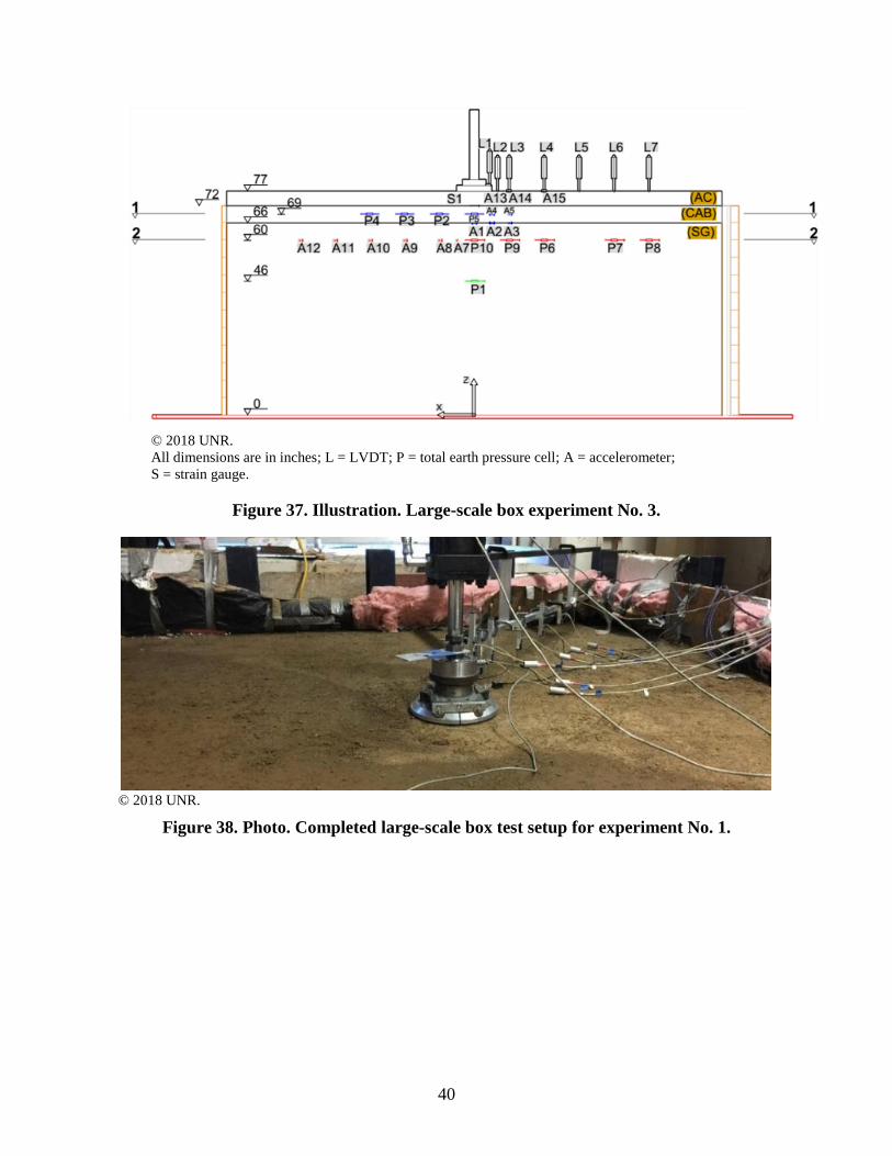
A12 A11 A10 A9 P6 P7 P8

P1

© 2018 UNR.


S = strain gauge.


© 2018 UNR.

Figure 38. Photo. Completed large-scale box test setup for experiment No. 1.

40

© 2018 UNR.


© 2018 UNR.


41

0.09

0.08 • ::E' "' CJ "' .5 0.07 "' '-' .... "' C: "' ~ 0.06 4 E ~ CJ "' ~ 0.05 "' Q. "' "' "' '5

~ ~ 0.04 CJ

"' ,;': "' !3 0.03 "' r:l.l ,,,,■ -;

CJ 0.02 "' :e . f ~

> 0.01

0 0 5,000 10,000 15,000 20,000 25,000 30,000

Applied Load (lb)

12.0

10.0 ■ , ,,. ,, Q

,,. "'

,,. 8 8.0

,,. "' ,,. .. "' ~ ,,. .0 ,,. r:l.l ,,. -; 6.0

,,. CJ ,,. 1i :e ,,. ~

,,. > ,,.

4.0 ,,. ,,. ■ ,,. ■

2.0

0.0 0 5,000 10,000 15,000 20,000 25,000 30,000

Applied Load (lb)

© 2018 UNR.

Figure 41. Graph. Vertical surface displacements measured by LVDT1 in experiment No. 3

at different load levels.

© 2018 UNR.

Figure 42. Graph. σv measured by TEPC1 in experiment No. 3 at different load levels.

The surface deflection basins at different load levels measured in these three experiments

(experiment Nos. 1, 2, and 3) were individually employed in the backcalculation process using

the program BAKFAA.(39) Subsequently, 3D-Move ENHANCED and the backcalculated layer

42

0

10 ,-.. ~

== 20 5 '-"

= 30 0 ~ y Q,l

40 i;:::: Q,l

0 Q,l 50 y

.;'.: I. 60 ::, r✓.l

70

80

90

Radial Distance (inch) 12 24 36 48 60

~ Load Level= 9,000 pound ....,Load Level= 12,000 pound ~ Load Level = 16,000 pound _._Load Level= 21,000 pound ~ Load Level= 27,000 pound

72

moduli were utilized to compute the pavement surface deflections and σv at the locations of

LVDTs and TEPCs, respectively.(11)

Figure 43 presents the deflection basins at each of the applied load levels in experiment No. 3.

Figure 44 and figure 45 depict the comparison of measured and calculated responses (i.e.,

surface deflection and σv, respectively) by 3D-Move ENHANCED using associated

backcalculated moduli.(11) These figures reveal the capability of this software to estimate the

load-induced surface deflections and stresses at interior locations. It should be noted that similar

conclusions are presented in Volume Ⅳ: Appendix C with the measurements from experiment

Nos. 1 and 2.(3)

© 2018 UNR.

Figure 43. Graph. Measured deflection basin in experiment No. 3.

43

0.10 ,-..,

-= 0.09 <..>

·= '-' 0.08 = .s .... 0.07 <..>

~ 4- 0.06 A '0 4-.... 0.05 s = 0.04 ~ ~

u 0.03 4-... 0

0.02 ~ I

A 0.01 !")

0.00 0.00

50

Q 45 VJ Q., '-' 40 VJ VJ 4-... ....

00 35

-~ 30 -~ .... ... 4-;> 25 '0 4-.... 20 s = 15 ~ ~ u 10 4-... 0

~ 5 I

A 0 !")

0 5

0.02

,,, ... ... ,,, +10 percent ,,, .. ,,, .. .. ,,, .. .. ,,, .. ,,, . . . .. ,,, .. .. ,,, .. .. .. ,, .. ,,, ,,, ,,, ,, ,,,

~ DO -•·D8 -~ D12 -• - D24 ~ - D36 ~ • D48 ~ · D60 · · · · ·· · Line of Equality

0.04 0.06 0.08 0.10

Measured Deflection (inch)

., ... ,,, .. + 10 percent. ,,, .... ♦· ·

; ...,: .<"· ,,,,, ,,,,, ; .,,,._. ,,,,,

,,,,. .,,,. .. ,,,,, ,,,,, ,,,,, . . . ,,,,, ,,,,, ,-.. ,,,,, ,,,,,, ,,,,. .. · ,,,,,

,,, .,,. ~--· - ,,,,, ,L_ .,. •• ' 10 ,,,_ ~.-: •. • · • .,. .,. - percent

t$, .., •• .,,,. .,,, ... •· .,, ,,,,, ,. .. .,,,. ~.,. .. • .. ~ .. ·· ; .,,,,.

~ .. ·· .. ,,,,, ,,, .. · ,,,,. .,,,.,,,,. ., .. • .,,,. -:x ~ Pl ,,,,, .,, " .. ··· "-;"/ ,,.,, ,, .. • ...... ,. ., .. ; .

- .. "'.•···.,,. -r.... , .. ,,-/4;'·✓--

10

, ~ '#t ..

15 20 25 30 35 Measured Vertical Stress (psi)

-~ PS

-• - P6 ~ - P9 -Ill· PIO

·•••••• Line of Equality

40 45 50

© 2018 UNR.

D = deflection.

Figure 44. Graph. Comparison between 3D-Move calculated deflections and measured

surface deflections in experiment No. 3.

© 2018 UNR.

P = total earth pressure cell.

Figure 45. Graph. Comparison between 3D-Move calculated σv and measured σv in

experiment No. 3.

44

3.2.2. Verification of SG τmax Parameters Estimation Procedure

The SG layer and c are necessary inputs for investigating the likelihood of ultimate and

localized shear failure as well as pavement shoulder slope stability under SHL movement. In this

study, an FWD-based procedure for estimating in situ τmax parameters of the SG was developed.

Detailed description of the procedure as well as verification using numerical modeling, large-

scale box experiments, and measurements from APTs are provided in Volume V: Appendix D.(4)

In this section, a summary of the verification process undertaken is presented.

It is known that FWD-load levels and the associated state of stresses in the SG layer do not reach

the failure state of the materials. The main concept behind this FWD-based procedure is to

extend the data obtained at lower stress levels to the failure state by implementing the nonlinear

hyperbolic stress–strain relationship of unbound material. This enables the estimation of df

(asymptotic value) and subsequent estimation of τmax parameters.

In this study, an extrapolation of the hyperbolic relationship using measured data at a lower state

of stresses was examined first by means of measured triaxial test results. To this end, the

available results of consolidated undrained triaxial tests without pore-water measurements

conducted on two different types of soils (i.e., clayey sand with gravel and Dupont clay) were

employed. For each set of triaxial test results, σd up to the cutoff levels of 20, 30, 40, and

50 percent of σdf and corresponding 1 were individually used to develop the linear form of the

hyperbolic relationship. Consequently, the estimated σdf using many sets of truncated data was

determined.

Figure 46 and figure 47 depict the estimated σdf normalized by the measured σdf (i.e., from

triaxial tests) for different cutoff levels of 20, 30, 40, and 50 percent of the measured σdf. It can

be seen that, at the cutoff level of 50 percent, the estimated σdf is reasonably close to the

measured value (i.e., less than 15 percent difference). Hence, it was concluded that when the

state of σd in a triaxial test reaches approximately 50 percent of σdf, the hyperbolic relationship

can be utilized to obtain the needed asymptotic value (i.e., σdf).

The validation process to investigate the feasibility of FWD measurements to estimate the

strength parameters was then continued by numerically simulating the FWD test using ILLI-

PAVE software.(38) The FWD measurements acquired from experiment Nos. 1, 2, and 3 were

also employed for the verification purpose and compared against the laboratory triaxial test

results. In addition, the FWD measurements conducted at NAPTF and LanammeUCR were

subsequently utilized.

45

100

90

C' 80 C ~

~ 70 "O ~

~ 5 60 ts: ~

.§ a 50 ..... = "' ts: ~ ~ 40

C' C ~ c., a..

"O ~ ~ Q. ..... __, ts: ~ E a.. ·- ::, ..... = "' ts: ~~ "O ..... ~ ts: ~ "' "' ts: ~ E !:: i.. r:,;i 0 a.. Z O .....

ts: ·5: ~

Cl

30

20

10

0

100

90

80

70

60

50

40

30

20

10

0

20% 30% 40% 50% 20% 30% 40% 50%

Percent Cutoff Levels ofDeviatoric Stress at Failure (Jc= 5 psi

<Jdf = 23 psi

20% 30% 40% 50%

I 20% 30% 40% 50%

(Jc= 10 psi <Jdf = 39.1 psi

20% 30% 40% 50%

Percent Cutoff Levels ofDeviatoric Stress at Failure

(Jc= 7 psi <Jdf = 12 psi



© 2018 UNR.


measured data for clayey sand with gravel.

© 2018 UNR.


measured data for Dupont clay.

A detailed presentation of the verification process for unpaved and paved pavement structures

can be found in Volume V: Appendix D.(4) Figure 48 represents the results of the verification

46

.,,, ,-._

.,,, ~

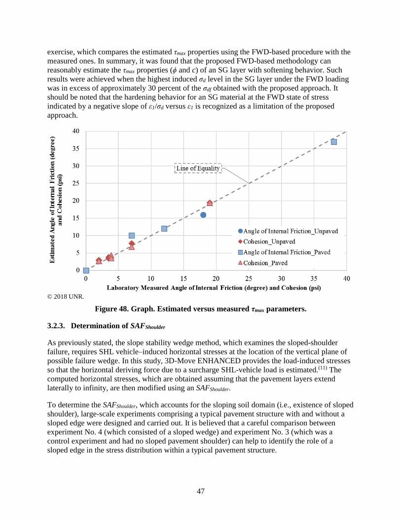
.,,, . ~ I-,

35 .,,,

~ .,,,

~ .,,,

-0 .,,,

'-' .,,,

C: .,,,

30 ~Lj~e_o_f ~9~a~i.!_Y_:~ .,,,.,,,,,,,.,,,.,,,

.,,, 0

::l

-~ =--r.. 8 25 .,,,

l .§ .,,, .,,, .,,,

~ "' 20 .,,, ... ~ . .,,, .s -§ .,,,

'o u .,,, .,,, • ~ -0 15 .,,, - C:

.,,, !~ .,,,

10 □ .,,, ..- e Angle of Internal Friction_Unpaved

-0 .,,, .,,,

~ .t .,,, ♦Cohesion_ Unpaved ... ~

.5 5 .... .,,, .,,, □Angle of Internal Friction_Paved ...

"' r..i .& Cohesion Paved 0

.,,,

0 5 10 15 20 25 30 35 40 Laboratory Measured Angle oflnternal Friction (degree) and Cohesion (psi)

exercise, which compares the estimated τmax properties using the FWD-based procedure with the

measured ones. In summary, it was found that the proposed FWD-based methodology can

reasonably estimate the τmax properties (ϕ and c) of an SG layer with softening behavior. Such

results were achieved when the highest induced σd level in the SG layer under the FWD loading

was in excess of approximately 30 percent of the σdf obtained with the proposed approach. It

should be noted that the hardening behavior for an SG material at the FWD state of stress

indicated by a negative slope of ε1/σd versus ε1 is recognized as a limitation of the proposed

approach.

© 2018 UNR.

Figure 48. Graph. Estimated versus measured τmax parameters.

3.2.3. Determination of SAFShoulder

As previously stated, the slope stability wedge method, which examines the sloped-shoulder

failure, requires SHL vehicle–induced horizontal stresses at the location of the vertical plane of

possible failure wedge. In this study, 3D-Move ENHANCED provides the load-induced stresses

so that the horizontal deriving force due to a surcharge SHL-vehicle load is estimated.(11) The

computed horizontal stresses, which are obtained assuming that the pavement layers extend

laterally to infinity, are then modified using an SAFShoulder.

To determine the SAFShoulder, which accounts for the sloping soil domain (i.e., existence of sloped

shoulder), large-scale experiments comprising a typical pavement structure with and without a

sloped edge were designed and carried out. It is believed that a careful comparison between

experiment No. 4 (which consisted of a sloped wedge) and experiment No. 3 (which was a

control experiment and had no sloped pavement shoulder) can help to identify the role of a

sloped edge in the stress distribution within a typical pavement structure.

47

Figure 49 and figure 50 illustrate the test setup for experiment No. 4. Detailed discussions

regarding the construction and instrumentation plan can be found in Volume Ⅱ: Appendix A.(1)

Similar to experiment No. 3, the pavement structure consisted of 5 inches of AC on top of

6 inches of CAB and 66 inches of SG soil. However, the pavement structure in experiment No. 4

included a side slope of 1:1.5 (33.7 degrees with the horizontal), and the surface FWD loading at

multiple levels was applied on top of the AC layer at three locations—12 inches (Loc12),

24 inches (Loc24), and 36 inches (Loc36)—from the edge of the slope. In this section, examples

of experimental measurements and exercises conducted to determine the SAFShoulder are

presented. Detailed descriptions and extensive discussion are provided in Volume: Ⅶ Appendix F.(6)

© 2018 UNR.

All dimensions are in inches; L = LVDT; P = total earth pressure cell; A = accelerometer; S = strain gauge.

Figure 49. Illustration. 3D view of large-scale box test setup for experiment No. 4.

48

8

16

0 14 "' Q., '-'

"' 12 "' Cl, ... ... rJ:j 10

,:o:i -~ ..... 8 ...

Cl,

> "O 6 Cl, ... = "' 4 ,:o:i Cl,

~ 2

0 5,000

,, ,,

,, ,, ,, ,, ...... --

,,' -,.- --,,,. - - - .L - - -

,, ..,, ..,, I y = 0.000483x I 1

R2 = 0.99 1

L------1

,----------, I Y = 0.000555X I I I I R2 = 0 95 I .,,' .... ____ -,-.;. ___ _. ,, ..

I " ,,_, ~,,

,, ,;..' ..,,

, --

■Exp No. 3 _P9

□Exp No. 4_Loc l2_P9

Exp No. 4_Loc24_P6

10,000 15,000 20,000 25 ,000 30,000 Applied Load (lb)

1

© 2018 UNR.


Figure 51 shows the measured σv in the SG on the nonslope side of the pavement structure with

respect to the location of the surface-applied load. In comparison with the corresponding

measured stresses in experiment No. 3, the stress distribution in the nonslope side of a pavement

structure was not affected by the sloped edge.

© 2018 UNR.


No. 3, nonslope side, 6 inches from SG surface, offset from the centerline of the load equal

to 12 inches.

49

18

<:::' 16 VJ Q.,

';' 14 VJ 4, ... 12 ...

00 -~ IO .l:= ... ...

4, 8 ;, ~ 4, 6 ... =

_, _,

_, _,

VJ ~ 4 4,

~ 2

0 5,000 10,000

, ~---_,

15,000

I y = 0.000695.x I I R2 = 0.99 I L------1

_, _, _,

_,[1"

20,000 Applied Load (lb)

, EJ _, _, _, _,

■Exp No. 3_Pl

□Exp No. 4_Locl2_Pl

25 ,000 30,000

20

Figure 52 represents the load-induced σv measured by the TEPCs, which were installed exactly

under the centerline of the load. A noticeable increase in the measured σv in experiment No. 4

compared to experiment No. 3 can be inferred from this figure.

© 2018 UNR.


No. 3, 20 inches from SG surface, centerline of the load.

Figure 53 depicts the measured σv at the location of TEPCs where they were located in the slope

side with respect to the applied surface load in experiment No. 4. In comparison to the matching

locations in experiment No. 3, substantially higher stresses were induced by the surface load,

which is attributed to the role of the sloped edge on the stress distribution. In summary, after

comprehensively reviewing and comparing the σv recorded in experiment Nos. 3 and 4, it was

concluded that the sloped shoulder plays a major role in the stress distribution within a pavement

structure, particularly in the slope side.

50

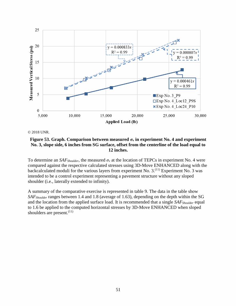
a- 20 "' Q., '-' <ll <ll ~

,:: 15 00

0

5,000

ig"'$

""'""' ig,-"""'

10,000

X .------------. ,,;r::j ly = 0.000833x I ,,-:;_..

I , _.. ""1 -------R2 = 0.99 : "7, , :,' _,. L I y = 0.000807x I

----1------ ..--:,;, 7 I •--~ ,,":(] L R2 = 0.99 1 'W, .,,,. ------; _, __

__M: , -;:- -,~~ ...

, ~ ,_..

15,000 20,000

Applied Load (lb)

■Exp No. 3 _P9 □Exp No. 4_Locl2_P9S ~ Exp No. 4_Loc24_Pl0

25 ,000 30,000

25

© 2018 UNR.


No. 3, slope side, 6 inches from SG surface, offset from the centerline of the load equal to

12 inches.

To determine an SAFShoulder, the measured σv at the location of TEPCs in experiment No. 4 were

compared against the respective calculated stresses using 3D-Move ENHANCED along with the

backcalculated moduli for the various layers from experiment No. 3.(11) Experiment No. 3 was

intended to be a control experiment representing a pavement structure without any sloped

shoulder (i.e., laterally extended to infinity).

A summary of the comparative exercise is represented in table 9. The data in the table show

SAFShoulder ranges between 1.4 and 1.8 (average of 1.63), depending on the depth within the SG

and the location from the applied surface load. It is recommended that a single SAFShoulder equal

to 1.6 be applied to the computed horizontal stresses by 3D-Move ENHANCED when sloped

shoulders are present.(11)

51

Loc12 IJIJIJIJDOOOOOOODO IJIJIJIJDDCJCJIJCJCJOOO IJIJIJIJDOOCJIJCJCJOIJO

FWD Loading Loc24

DCJOCCIJIJIJIJIJDDOO DCJDCIJIJIJIJIJIJDDOO CJCJCCCIJIJIJIJIJCOCJCJ

AC La er CAB Layer

SG Layer

Horizontal Boundaries of Wedges

Loc36 OODIJIJIJIJIJIJIJIJIJDD OOIJIJIJCICICICICICICCICJ o a a a a i:u::u::u::u::u::u::i cc

5 inch

6 inch

66 rnch

Table 9. Summary of comparison between stresses measured in experiment No. 4 and

computed by 3D-Move Analysis software.

Pressure Cell

Depth From the

SG Surface

(Inches)

Surface-Load

Location in

Experiment No. 4

Offset From

Centerline of the

Load (Inches) SAFShoulder

P1 20 Loc12 0 1.4

P10 6 Loc12 0 1.8

P1 20 Loc24 12 1.6

P1 20 Loc36 24 1.6

P9S 6 Loc12 12 1.6

P10 6 Loc24 12 1.6

P10 6 Loc36 24 1.8

3.2.4. Verification of Sloped-Shoulder Failure Analysis Procedure

To evaluate the applicability of the proposed slope stability analysis using the wedge method, the

FOS of the sloping edge in experiment No. 4 was determined when the FWD loads were applied

at three locations (i.e., Loc12, Loc24, and Loc36). Figure 54 shows an illustration of the

pavement structure and loading locations in experiment No. 4. As shown in this figure, different

failure wedges with horizontal and inclined slip surfaces were considered.

© 2018 UNR.

Figure 54. Illustration. Schematic of experiment No. 4.

The wedge method assumes plane strain condition for the slope stability analysis under the SHL

vehicle since the length of SHL vehicles usually extends to a relatively large extent. However, in

experiment No. 4, the FWD load was applied on the 11.9-inch circular plate, which means that

the plane strain assumption does not hold true. Therefore, the wedge method was reformulated to

account for the 3D domain present, which is described in Volume Ⅶ: Appendix F.(6) Figure 55

illustrates the possible 3D failure wedge as well as the force diagram in experiment No. 4 where

the width of the wedge (Bwedge) equal to 11.9 inches (i.e., width of the FWD plate) was assumed.

52

Wedge =11.9 ·nch

CAB Layer

SG Layer

© 2018 UNR.

T’D = developed resisting cohesion force resulting from mobilized cohesion acting on the side surfaces (i.e., front

and back); PD = resistive force from the side soil that makes an angle ϕD with the normal to the side surfaces (i.e.,

front and back).

Figure 55. Illustration. Force diagram applied on the possible failure wedge.

In this verification exercise, the highest FWD-load level (approximately 27,000 lb), which was

applied at the aforementioned three locations, was considered. As for Loc12, a minimum FOS

equal to 1.3 was determined for the possible failure wedge where the horizontal slip surface is

located 3 inches from the SG surface (i.e., 14 inches from the pavement surface). When the FWD

load was applied at Loc24 and Loc36, minimum FOS equal to 1.6 and 3.1, respectively, were

determined. It should be mentioned that slope failure was not observed for the same loading

cases in experiment No. 4, confirming that the proposed application of the wedge method is

capable of assessing the stability of a sloping layered medium consisting of a typical pavement-

layer configuration and properties.

3.2.5. Determination of SAFUtility

Reliable risk analysis against failure of existing buried utilities due to an SHL-vehicle movement

on a flexible pavement can only be achieved by appropriately assessing the SHL vehicle– induced stresses at the location of the buried utility. To this end, the computed σv by 3D-Move

ENHANCED, in conjunction with the modification using SAFUtility, was implemented.(11)

To determine the SAFUtility that accounts for the role of soil–structure interaction and

discontinuities within the medium (i.e., existence of buried utilities), full-scale experiments

comprising a typical pavement structure (i.e., experiment Nos. 3 and 5) were designed and

carried out. As previously described, experiment No. 3 is considered the control experiment

without any cavities (i.e., no buried utilities). Experiment No. 5 represents a similar pavement

structure, including two types of buried utilities (flexible steel pipe and rigid concrete box

culvert), which were installed in the SG (figure 56). Surface FWD loads at multiple intensities

were applied directly above the centerlines of the buried utilities. Figure 57 and figure 58

illustrate the test setup for experiment No. 5. Detailed discussions regarding the construction and

instrumentation plan are presented in Volume Ⅱ: Appendix A.(1) In this section, the process to

determine SAFUtility along with the important observations from experiment No. 5 are presented.

Volume Ⅶ: Appendix F provides extensive discussion on this matter.(6)

53

♦ -t

6 inch

77 inch

® Dynarric and Increasing Static Load Application

© ® 11.9 inch Plate t 7 application

Pave Box

12 inch Steel Pipe thickness= 1/8 inch

12x12x1 inch Concrete Box Culvert

© 2018 UNR.

Figure 56. Photo. Buried flexible steel pipe and rigid concrete box culvert in experiment

No. 5.

© 2018 UNR.

Figure 57. Illustration. Schematic of the test setup for experiment No. 5.

54

© 2018 UNR.

Figure 58. Illustration. 3D view of large-scale box test setup for experiment No. 5.

In experiment No. 5, TEPCs were installed at the top and bottom of the buried pipe and culvert

to capture induced stresses due to surface loads. Data obtained from these TEPCs were compared

with data obtained from TEPCs from experiment No. 3 installed at the same locations and

depths.

Figure 59 shows the measured load-induced σv by the TEPCs installed at the top of the buried

utilities when the FWD loads were applied at the centerline of the corresponding buried utility.

As shown in this figure, the σv experienced by the flexible pipe are much lower than those

stresses distributed in experiment No. 3 when buried utilities were not present. However, the

load-induced σv in experiment No. 5 recorded at the top of the rigid culvert are higher than the

measurements in experiment No. 3.

Figure 60 shows the measured σv by TEPCs installed at the bottom of the buried utilities in

experiment No. 5 and the TEPCs located at the same depth and location in experiment No. 3 as a

function of applied surface load. As shown, there is not much change in the stresses due to the

presence of the flexible pipe. One possible explanation for this observation is that the presence of

the flexible pipe redistributed the stresses and affected the stress flow near and around the pipe.

However, substantially lower σv at the bottom of concrete culvert compared to the corresponding

measurements in experiment No. 3 were observed. These observations can be attributed to the

soil–structure interaction and higher rigidity (i.e., stiffness) of concrete culvert with respect to the

surrounding SG soil.

55

30.0

25 .0

Q ~

5 20.0 ~ ~

~ ... .... 00 15 .0 ';j ~

:0 ... ~

10.0 ;..

5.0

0.0 0

12.0

0.0 0

e Exp. No. 3_No Buried Utility -·-■Flexible Pipe

.&. Rigid Culvert

5,000

.,, .... • A"

.... , .. , ..

.,.

... .... .. .. ..... .. Ji,.-. .. ,- ......

.,. .... , .... ....

, .........

.. - --- - - --- - - - --- - - - - -II

10,000 15,000 20,000 25,000 Applied Load (lb)

e Exp. No. 3_No Buried Utility

5,000

... - .Jr. - ·--·-· . -• -. -10,000 15,000 20 ,000

Applied Load (lb)

- . _,, .....

25,000

30,000

30,000

© 2018 UNR.

Figure 59. Graph. Measured σv in experiment No. 3 and top of buried utilities in

experiment No. 5.

© 2018 UNR.

Figure 60. Graph. Measured σv in experiment No. 3 and bottom of buried utilities in

experiment No. 5.

The aforementioned observations revealed that the existence of buried utilities in the pavement

structure significantly influences the stress distribution within the pavement layers, indicating a

56

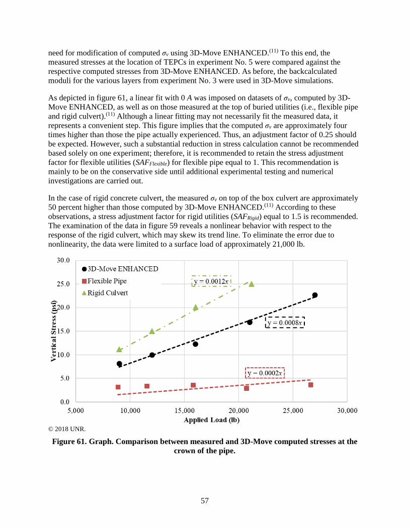
25.0

0 ~0.0 '-'

"' "' ~ ~15.0 ~

-~ .... ~10.0

5.0

e 3D-Move ENHANCED

■Flexible Pipe iJ_=_0:~!2.: ! • ___... • Rigid Culve1t ,,,.

,,,. ...... ...... ...... ,,,. .......

L • .,.,' - ...... ...... ...... ~---

,,,.

...... ...... ......

......

... --, - - - - - ., ......... ... .. i1: ~~~-:.'

1--------- I I Y = 0.0002x I L---------~

... •

-------.. ---. . . --------.- . -----------------0.0

5,000 10,000 15,000 20 ,000 25,000 Applied Load (lb)

30,000

need for modification of computed σv using 3D-Move ENHANCED.(11) To this end, the

measured stresses at the location of TEPCs in experiment No. 5 were compared against the

respective computed stresses from 3D-Move ENHANCED. As before, the backcalculated

moduli for the various layers from experiment No. 3 were used in 3D-Move simulations.

As depicted in figure 61, a linear fit with 0 A was imposed on datasets of σv, computed by 3D-

Move ENHANCED, as well as on those measured at the top of buried utilities (i.e., flexible pipe

and rigid culvert).(11) Although a linear fitting may not necessarily fit the measured data, it

represents a convenient step. This figure implies that the computed σv are approximately four

times higher than those the pipe actually experienced. Thus, an adjustment factor of 0.25 should

be expected. However, such a substantial reduction in stress calculation cannot be recommended

based solely on one experiment; therefore, it is recommended to retain the stress adjustment

factor for flexible utilities (SAFFlexible) for flexible pipe equal to 1. This recommendation is

mainly to be on the conservative side until additional experimental testing and numerical

investigations are carried out.

In the case of rigid concrete culvert, the measured σv on top of the box culvert are approximately

50 percent higher than those computed by 3D-Move ENHANCED.(11) According to these

observations, a stress adjustment factor for rigid utilities (SAFRigid) equal to 1.5 is recommended.

The examination of the data in figure 59 reveals a nonlinear behavior with respect to the

response of the rigid culvert, which may skew its trend line. To eliminate the error due to

nonlinearity, the data were limited to a surface load of approximately 21,000 lb.

© 2018 UNR.

Figure 61. Graph. Comparison between measured and 3D-Move computed stresses at the

crown of the pipe.

57

..... , __ _

. -.. '

~J!~· · ... ~ l

),

3.2.6. Verification of Buried Utility Risk Analysis Procedure

As previously noted, the analysis procedure to investigate the risk against the failure of existing

buried utilities under an SHL-vehicle movement was adopted from existing well-established

state of practices with a modification to stress distribution. Experiment No. 5 also provided

insight into the behavior of the buried utilities under surface loading on a typical pavement

structure.

In experiment No. 5, as demonstrated in figure 62, perpendicular LVDTs were installed inside

the pipe under the centerline of the load to capture the horizontal and vertical deformation

(change in pipe diameter). Figure 63 presents the vertical and horizontal deformations in the pipe

cross section as a function of surface-load levels. The negative sign indicates that the deflection

is inward, which means that the pipe diameter in the vertical direction was decreasing with load.

As shown, the horizontal direction response is exactly the same but in opposite directions,

leading to the conclusion that the pipe remained elastic during the load application (i.e., no

yielding).

Data from the vertical LVDT were used to calculate pipe ovality, which is defined as the ratio of

vertical deflection in the pipe cross section to the pipe diameter. As presented in figure 63, the

maximum deflection was approximately 0.041 inch at a surface load of 26,631 lb. This translates

to an ovality of 0.34 percent. Given the fact that some of the material properties associated with

the flexible pipe (modulus of steel pipe, bedding factors, etc.) were assumed, the backcalculated

σv of 1.3 psi at the crown of the pipe to cause such ovality is reasonably close to the measured

stress of 3.7 psi.

© 2018 UNR.

Figure 62. Photo. Four LVDTs installed inside the buried steel pipe at the centerline of the

pipe and 12 inches off the center of the pipe.

58

.c

0.05

0.04

0.03

0.02

~ 0.01 C

§ 0.00 :::I

~ -0 01 i;:::: . ~

Cl -0.02 ~ Q.,

0:: -0.03

-0.04

-0.05

• Vertical Deflection

■Horizontal Deflection

t- ----- ---·----------

5,000 10,000 15,000 20,000 Applied Load (lb)

--· --- -- -- --

25,000 30,000

© 2018 UNR.

Figure 63. Graph. Vertical and horizontal deformations in pipe cross section.

To investigate the internal integrity of the buried concrete culvert in experiment No. 5, structural

analysis was conducted with knowledge of the characteristics of the concrete culvert. The

adjusted computed σv on top of the concrete culvert using 3D-Move ENHANCED was used.(11)

Analyses of flexural strength, τmax, and axial thrust for the members (i.e., top slab, bottom slab,

and sidewalls) at different load levels revealed that the concrete culvert is structurally adequate at

all FWD-load levels in terms of τmax and axial thrust. However, at the highest FWD surface

loading (i.e., 27,000 lb), the maximum induced moment (Mu) in the members is higher than their

flexural capacity (i.e., factored flexural resistance (ϕfMn)), indicating a possibility of failure. Such

an observation is consistent with the nonlinear behavior of rigid culvert response where the

measured σv on top of the culvert at the highest FWD-load level of 27,000 lb indicated a visible

skew in trend (figure 59). It should be noted that the concrete culvert was purposely designed in

a way to experience distress at the high load levels of surface FWD loading.

59

CHAPTER 4. SHL CASE STUDIES

To demonstrate the developed methodology to evaluate SHL movements on flexible pavement,

two SHL-vehicle configurations permitted by the Louisiana Department of Transportation and

Development (LaDOTD) were investigated. The pavement structure at the APT facility in

LanammeUCR was assumed for the two vehicles’ route. For this flexible pavement structure,

supplementary laboratory test results as well as FWD measurements were available. In this

chapter, the analyses steps and a summary of the analysis results associated with the procedures

developed are provided.

4.1. SHL ANALYSIS VEHICLES CONFIGURATIONS

The axle and tire configurations for the two SHL-vehicle cases under consideration (LA-12T-16,

figure 2, and LA-8T-14, figure 1) are summarized in table 10. The LA-12T-16 SHL vehicle

consisted of four identical dollies, and the spacing between the dollies was approximately 38 ft.

The LA-8T-14 SHL vehicle consisted of 28 similar axles that were uniformly distributed at a

spacing of 4 ft and 7 inches along the entire length of the SHL vehicle. A vehicle traveling speed

of 10 mph was assumed for both cases.

Table 10. Summary of SHL-vehicle characteristics from Louisiana sample permits.

Load Case

No.

GVW

(lb)

Number

of

Axles

Number

of Tires

per Axle

Axle Width

(Inches)

Center-to-Center

Distance Between

Adjacent Axles

(Inches)

Tire

Load

(lb)

LA-12T-16 1,754,220 24 12 20913/16 571/16 6,164

LA-8T-14 3,660,552 28 8 20913/16 571/16 16,342

4.2. PAVEMENT STRUCTURE AND MATERIAL PROPERTIES

The thickness of the LanammeUCR pavement layers that were used in this exercise is shown in

table 11. The viscoelastic properties of the AC layer, characterized using E* laboratory data as a

function of temperature and frequency, are presented in table 12 and table 13. It should be noted

that E* tests were conducted on the field-mixed laboratory-compacted specimens that are

assumed to be representative of the AC-layer properties at the time of SHL movements.

Knowing that the viscosity grading of the asphalt binder in the AC mixture was AC-30, the

viscostiy–temperature susceptibility parameters (i.e., A and VTS) equal to 10.6316 and −3.548

were assumed, respectively.

Table 11. Flexible pavement structure: Layer thicknesses.

Layer Thickness (Inch)

AC 5

Unbound CAB 9.5

Unbound subbase 12

SG 72

61

Distance (inch) 0 10 20 30 40 50 60 70 80

0

5 ,-,, "' = E '-'

10 C 0 .::

15 '-I ~

i;:::: ~

0 20 ~

'-I

~ I. ::I 25 00

30 ------------ ~ Load Level= 9,000 pound ~ Lo ad Level= 12,000 pound ~ Load Level= 16,000 pound

35

Table 12. E* values for the AC layer in psi.

Temperature

(°F) 0.1 Hz 0.5 Hz 1 Hz 5 Hz 10 Hz 25 Hz

40 1,176,000 1,514,000 1,670,000 2,027,000 2,186,000 2,398,000

70 312,800 510,800 614,300 910,000 1,057,000 1,263,000

100 57,600 117,800 15,4100 290,600 365,200 487,000

130 11,600 20,700 27,800 63,900 90,400 140,000

Table 13. Phase angle values for the AC layer in degrees.

Temperature

(°F) 0.1 Hz 0.5 Hz 1 Hz 5 Hz 10 Hz 25 Hz

40 16.75 13.51 12.36 10.15 9.40 8.53

70 30.76 27.04 25.63 21.37 19.75 17.76

100 33.75 34.45 34.93 32.39 31.43 29.73

130 25.07 29.11 31.63 33.30 34.47 36.14

The backcalculated moduli of unbound materials using the available FWD measurements

collected immediately after construction were utilized in this exercise. Figure 64 depicts the

deflection measurements (i.e., deflection basins) at three target FWD-load levels of 9,000,

12,000, and 16,000 lb. It should be noted that, during the assessment of the methodology

developed, FWD measurements at higher load levels were needed for given pavement structures

to generate state of stresses comparable to those induced under an SHL vehicle.

© 2018 UNR.

Figure 64. Graph. Vertical and horizontal deformations in pipe cross section.

To undertake the backcalculation process, BAKFAA open-source software was utilized.(39)

Repeated attempts at the backcalculation process with many controls on the variability of the

62

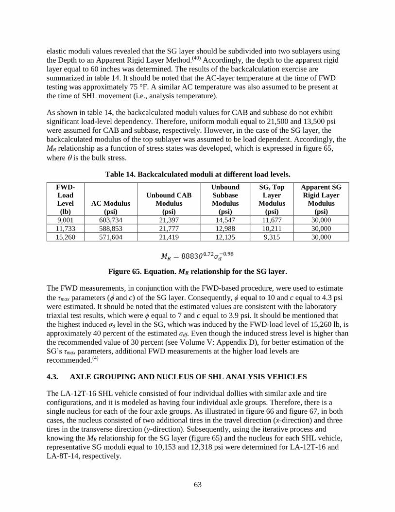
elastic moduli values revealed that the SG layer should be subdivided into two sublayers using

the Depth to an Apparent Rigid Layer Method.(40) Accordingly, the depth to the apparent rigid

layer equal to 60 inches was determined. The results of the backcalculation exercise are

summarized in table 14. It should be noted that the AC-layer temperature at the time of FWD

testing was approximately 75 °F. A similar AC temperature was also assumed to be present at

the time of SHL movement (i.e., analysis temperature).

As shown in table 14, the backcalculated moduli values for CAB and subbase do not exhibit

significant load-level dependency. Therefore, uniform moduli equal to 21,500 and 13,500 psi

were assumed for CAB and subbase, respectively. However, in the case of the SG layer, the

backcalculated modulus of the top sublayer was assumed to be load dependent. Accordingly, the

MR relationship as a function of stress states was developed, which is expressed in figure 65,

where is the bulk stress.

Table 14. Backcalculated moduli at different load levels.

FWD-

Load

Level

(lb)

AC Modulus

(psi)

Unbound CAB

Modulus

(psi)

Unbound

Subbase

Modulus

(psi)

SG, Top

Layer

Modulus

(psi)

Apparent SG

Rigid Layer

Modulus

(psi)

9,001 603,734 21,397 14,547 11,677 30,000

11,733 588,853 21,777 12,988 10,211 30,000

15,260 571,604 21,419 12,135 9,315 30,000

Figure 65. Equation. MR relationship for the SG layer.

The FWD measurements, in conjunction with the FWD-based procedure, were used to estimate

the τmax parameters ( and c) of the SG layer. Consequently, ϕ equal to 10 and c equal to 4.3 psi

were estimated. It should be noted that the estimated values are consistent with the laboratory

triaxial test results, which were ϕ equal to 7 and c equal to 3.9 psi. It should be mentioned that

the highest induced σd level in the SG, which was induced by the FWD-load level of 15,260 lb, is

approximately 40 percent of the estimated σdf. Even though the induced stress level is higher than

the recommended value of 30 percent (see Volume Ⅴ: Appendix D), for better estimation of the

SG’s τmax parameters, additional FWD measurements at the higher load levels are (4) recommended.

4.3. AXLE GROUPING AND NUCLEUS OF SHL ANALYSIS VEHICLES

The LA-12T-16 SHL vehicle consisted of four individual dollies with similar axle and tire

configurations, and it is modeled as having four individual axle groups. Therefore, there is a

single nucleus for each of the four axle groups. As illustrated in figure 66 and figure 67, in both

cases, the nucleus consisted of two additional tires in the travel direction (x-direction) and three

tires in the transverse direction (y-direction). Subsequently, using the iterative process and

knowing the MR relationship for the SG layer (figure 65) and the nucleus for each SHL vehicle,

representative SG moduli equal to 10,153 and 12,318 psi were determined for LA-12T-16 and

LA-8T-14, respectively.

63

250

• • • • -fi 200 • • • • C: = C: • Q 0 ~ 150

• • • • "O ' >,

s c,,

·§ 100

"' • .... Target tire • • a. <I)

-;;, • • • • ~ ;:: 50

• • • • 50 100 150 200 250

nre(s) spacing in x-direction (inch)

200

180 • • • • -fi 160 C: • • • • = § 140

ti • • • • -~ 120 "O >, .£: 100 • --Target Ire • • en C: ·u 80

"' • • • • a. VJ

60 -;;, QJ ~ 40 i= • • • • 20

50 100 150 200 250

Tire(s) spacing in x-direction (inch)

© 2018 UNR.

Figure 66. Graph. Representative nucleus for LA-12T-16 SHL vehicle.

© 2018 UNR.

Figure 67. Graph. Representative nucleus for LA-8T-14 SHL vehicle.

64

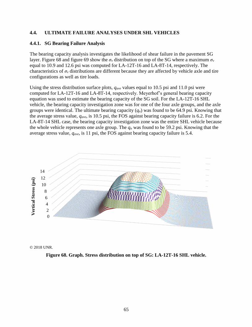
0

2

4

6

8

0-2 2-4 4-6 6-8 8-10 10-12 12-14

/

,,/ ,, ,, ,, / ,, / ,, ,, / ,

/ /

/

II' ~

IE ◊

•

4.4. ULTIMATE FAILURE ANALYSES UNDER SHL VEHICLES

4.4.1. SG Bearing Failure Analysis

The bearing capacity analysis investigates the likelihood of shear failure in the pavement SG

layer. Figure 68 and figure 69 show the σv distribution on top of the SG where a maximum σv

equal to 10.9 and 12.6 psi was computed for LA-12T-16 and LA-8T-14, respectively. The

characteristics of σv distributions are different because they are affected by vehicle axle and tire

configurations as well as tire loads.

Using the stress distribution surface plots, qave values equal to 10.5 psi and 11.0 psi were

computed for LA-12T-16 and LA-8T-14, respectively. Meyerhof’s general bearing capacity

equation was used to estimate the bearing capacity of the SG soil. For the LA-12T-16 SHL

vehicle, the bearing capacity investigation zone was for one of the four axle groups, and the axle

groups were identical. The ultimate bearing capacity (qu) was found to be 64.9 psi. Knowing that

the average stress value, qave, is 10.5 psi, the FOS against bearing capacity failure is 6.2. For the

LA-8T-14 SHL case, the bearing capacity investigation zone was the entire SHL vehicle because

the whole vehicle represents one axle group. The qu was found to be 59.2 psi. Knowing that the

average stress value, qave, is 11 psi, the FOS against bearing capacity failure is 5.4.

Ver

tica

l S

tres

s (p

si)

14

12

10

© 2018 UNR.

Figure 68. Graph. Stress distribution on top of SG: LA-12T-16 SHL vehicle.

65

14

~ 12 Q. .._,

"' "' q,J ... .... 00

10

8

6

4

2

0

Shoulder I Edge of

t 0-2 ,.. 2-4 II 4-6 o, 6-8 l+ 8-10 ◊ 10-12 ■ 12-14

I Travel Lane SHL Vehicle 1 1211~=-~

SG Layer SG Layer

© 2018 UNR.

Figure 69. Graph. Stress distribution on top of SG: LA-8T-14 SHL vehicle.

4.4.2. Sloped-Shoulder Failure Analysis Under LA-8T-14

The sloped-shoulder failure analysis using the wedge method was undertaken for the SHL

vehicle LA-8T-14, traveling on the selected pavement structure that includes a side slope of 1:1.5

(33.7 degrees with the horizontal). As shown in figure 70, the pavement layers are assumed to

extend into the shoulder. In addition, the clearance between the edge of the most outer tire and

sloped edge equal to 48 inches was assumed.

© 2018 UNR.

Figure 70. Illustration. Pavement structure with sloped pavement shoulder, side slope of

1:1.5.

66

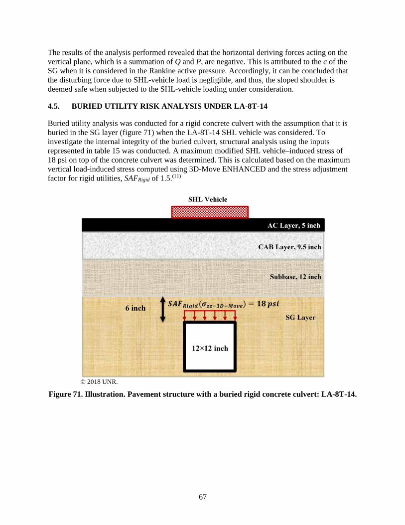
HL Vehicle

Subbase, 12 inch

6 inch t SAF Rinid (<Tzz- 3D- Move) = 18 psi

SG Layer

12x12 inch

The results of the analysis performed revealed that the horizontal deriving forces acting on the

vertical plane, which is a summation of Q and P, are negative. This is attributed to the c of the

SG when it is considered in the Rankine active pressure. Accordingly, it can be concluded that

the disturbing force due to SHL-vehicle load is negligible, and thus, the sloped shoulder is

deemed safe when subjected to the SHL-vehicle loading under consideration.

4.5. BURIED UTILITY RISK ANALYSIS UNDER LA-8T-14

Buried utility analysis was conducted for a rigid concrete culvert with the assumption that it is

buried in the SG layer (figure 71) when the LA-8T-14 SHL vehicle was considered. To

investigate the internal integrity of the buried culvert, structural analysis using the inputs

represented in table 15 was conducted. A maximum modified SHL vehicle–induced stress of

18 psi on top of the concrete culvert was determined. This is calculated based on the maximum

vertical load-induced stress computed using 3D-Move ENHANCED and the stress adjustment

factor for rigid utilities, SAFRigid of 1.5.(11)

© 2018 UNR.

Figure 71. Illustration. Pavement structure with a buried rigid concrete culvert: LA-8T-14.

67

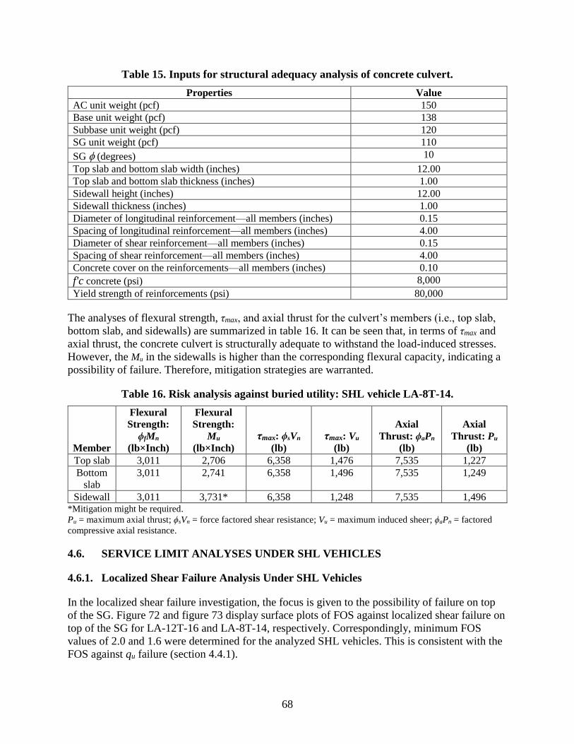
Table 15. Inputs for structural adequacy analysis of concrete culvert.

Properties Value

AC unit weight (pcf) 150

Base unit weight (pcf) 138

Subbase unit weight (pcf) 120

SG unit weight (pcf) 110

SG (degrees) 10

Top slab and bottom slab width (inches) 12.00

Top slab and bottom slab thickness (inches) 1.00

Sidewall height (inches) 12.00

Sidewall thickness (inches) 1.00

Diameter of longitudinal reinforcement—all members (inches) 0.15

Spacing of longitudinal reinforcement—all members (inches) 4.00

Diameter of shear reinforcement—all members (inches) 0.15

Spacing of shear reinforcement—all members (inches) 4.00

Concrete cover on the reinforcements—all members (inches) 0.10

f'c concrete (psi) 8,000

Yield strength of reinforcements (psi) 80,000

The analyses of flexural strength, τmax, and axial thrust for the culvert’s members (i.e., top slab,

bottom slab, and sidewalls) are summarized in table 16. It can be seen that, in terms of τmax and

axial thrust, the concrete culvert is structurally adequate to withstand the load-induced stresses.

However, the Mu in the sidewalls is higher than the corresponding flexural capacity, indicating a

possibility of failure. Therefore, mitigation strategies are warranted.

Table 16. Risk analysis against buried utility: SHL vehicle LA-8T-14.

Member

Flexural

Strength:

ϕfMn

(lb×Inch)

Flexural

Strength:

Mu

(lb×Inch)

τmax: ϕsVn

(lb)

τmax: Vu

(lb)

Axial

Thrust: ϕaPn

(lb)

Axial

Thrust: Pu

(lb)

Top slab 3,011 2,706 6,358 1,476 7,535 1,227

Bottom

slab

3,011 2,741 6,358 1,496 7,535 1,249

Sidewall 3,011 3,731* 6,358 1,248 7,535 1,496 *Mitigation might be required.

Pu = maximum axial thrust; ϕsVn = force factored shear resistance; Vu = maximum induced sheer; ϕaPn = factored

compressive axial resistance.

4.6. SERVICE LIMIT ANALYSES UNDER SHL VEHICLES

4.6.1. Localized Shear Failure Analysis Under SHL Vehicles

In the localized shear failure investigation, the focus is given to the possibility of failure on top

of the SG. Figure 72 and figure 73 display surface plots of FOS against localized shear failure on

top of the SG for LA-12T-16 and LA-8T-14, respectively. Correspondingly, minimum FOS

values of 2.0 and 1.6 were determined for the analyzed SHL vehicles. This is consistent with the

FOS against qu failure (section 4.4.1).

68

FOS(roinirouo1) = 2.0

3.00

2.75

2.50 00 0 2.25 r..

2.00

1.75 1.50

FOS(OllllimUDl) = 1.6

6.00

5.00

4.00 00 0 3.00 r..

2.00

1.00

0.00

i) 1.50-1.75 ~ 1.75-2.00 s 2.00-2.25 11 2.25-2.50 -~ 2.50-2. 75 ■ 2.75-3.00

:m 0.00-1.00 ~ 1.00-2.00 ~ 2.00-3.00 ■ 3.00-4.00 :-: 4.00-5.00 ■ 5.00-6.00

© 2018 UNR.

Figure 72. Graph. FOS against localized shear failure: LA-12T-16 SHL vehicle.

© 2018 UNR.

Figure 73. Graph. FOS against localized shear failure: LA-8T-14 SHL vehicle.

4.6.2. Deflection-Based Service Limit Analysis Under SHL Vehicles

The focus of the deflection-based service limit analysis is to avoid excessive surface deflections

under the SHL analysis vehicle movements. This is achieved by checking the SHL vehicle– induced deflections against a certain allowable surface defection. As shown in figure 74 and

69

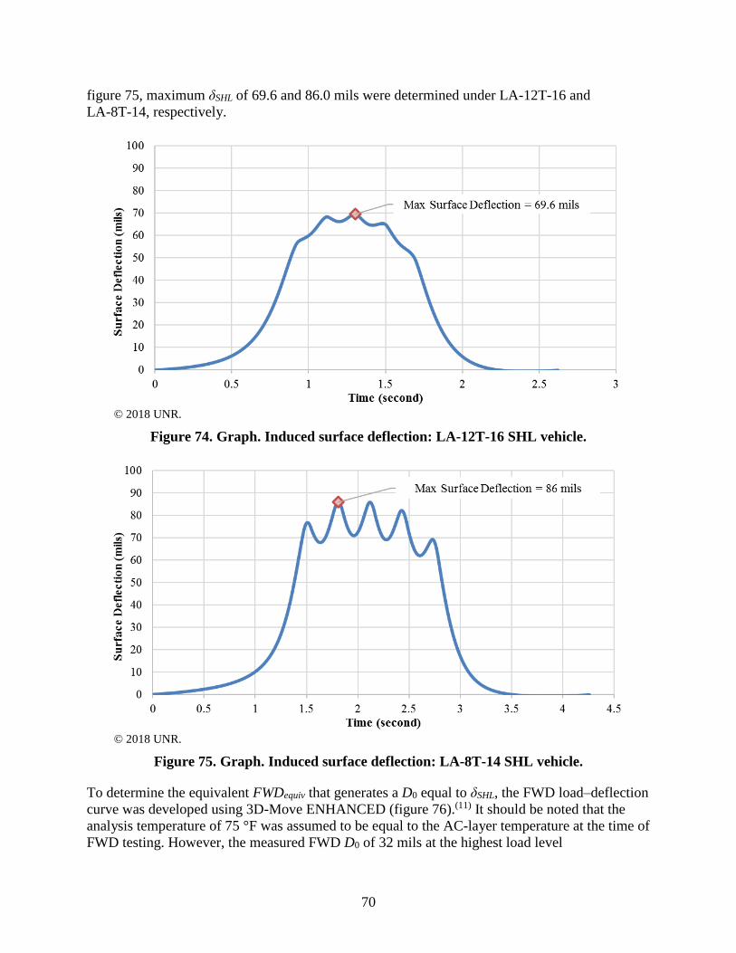
,,..., "' s '-' C 0 ; ... ., !;:: ., Q Cl,) ... ~ .. ::, rJl

100

90

80

70

60

50

40

30

20

10

0

100

90

80

';;' 70 = ,$ 60 C 0

~ 50 ., ~ 40 Q .,

30 ... ~ ..

20 ::, rJl

10

0

0 0.5

0 0.5 1.5

Max Surface Deflection= 69.6 mils

1.5 2 2.5 3 Time (second)

Max Surface Deflection = 86 mils

2 2.5 3 3.5 4 4.5 Time (second)

figure 75, maximum δSHL of 69.6 and 86.0 mils were determined under LA-12T-16 and

LA-8T-14, respectively.

© 2018 UNR.

Figure 74. Graph. Induced surface deflection: LA-12T-16 SHL vehicle.

© 2018 UNR.

Figure 75. Graph. Induced surface deflection: LA-8T-14 SHL vehicle.

To determine the equivalent FWDequiv that generates a D0 equal to δSHL, the FWD load–deflection

curve was developed using 3D-Move ENHANCED (figure 76).(11) It should be noted that the

analysis temperature of 75 °F was assumed to be equal to the AC-layer temperature at the time of

FWD testing. However, the measured FWD D0 of 32 mils at the highest load level

70

90 ... • 80

... ---

... "' ¥ e 70 ,_,, C 0 60 :0 C'j ~

Po: 50 ~

Q ... ~ 40 ... C'j ... .;::

30 ... • I.

= ... rJl

~ 20 18-wheel truck ~ 10 " FWD equiv = 8,000 lb

0 0 5,000 10,000 15 ,000 20,000 25,000 30,000 35 ,000 40,000 45,000

FWD Load Level (lb)

(approximately 16,000 lb) was lower than the calculated δSHL values of 69.6 and 86 mils under

the SHL vehicles. To extend the FWD deflections beyond the measured values, higher FWD-

load levels (beyond 16,000 lb) were considered in the 3D-Move ENHANCED analysis. In these

calculations, the backcalculated moduli of the pavement layers were used. In figure 65, the

modulus of the top SG layer for each load level under consideration was iteratively estimated

knowing the MR relationship. As shown in figure 76, FWDequiv equal to 31,000 and 37,500 lb for

LA-12T-16 and LA-8T-14 were determined, respectively. These FWD-load levels correspond to

the determined δSHL of 69.6 and 86.0 mils that were induced by SHL vehicles.

Similar steps were undertaken to determine the surface deflection under a typical 18-wheel truck

with GVW of 80,000 lb, one steering axle weighing 12,000 lb, and two tandem axles each

weighing 34,000 lb. Accordingly, a maximum surface deflection equal to 14.3 mils was

determined under the tandem axle using 3D-Move ENHANCED.(11) As depicted in figure 76,

this surface deflection corresponds to an FWDequiv of 8,000 lb.

Using the FWD load–SSR curve (figure 77), an FWDallow of 26,000 lb corresponding to an SSR

of 0.7 was determined. The determined FWDequiv values for both SHL vehicles were above

26,000 lb, indicating potential accumulation of unacceptable levels of permanent surface

deformation. These observations reveal that mitigation strategies are warranted for both of the

SHL analysis vehicles.

© 2018 UNR.

Figure 76. Graph. Developed FWD load–deflection curve.

71

0.9

Cl.& SSR~0.7

0.7 _ ....... _ ..... --...---..... ------a. ..._,,

().6

i:r: 0.5 tn rn

0.4

0.3

0.2 F\VD111o,t., = 26,000 lb

0.1

0 0 S,000 10 000 ]5 ,000 20 000 25 ,000 0.000 35 ,000 40.000 45 ,000

F WD o, d e 'el ( lb),

© 2018 UNR.

Figure 77. Graph. Developed FWD load–SSR curve.

4.7. COST ALLOCATION ANALYSIS: LA-12T-16 AND LA-8T-14

To conduct the cost analysis associated with pavement damage for the two analyzed SHL

movements, the assumptions presented in table 17 were made. It needs to be noted that the

analysis was conducted based on the MEPDG nationally calibrated factors for both AC

permanent deformation and AC fatigue cracking. In addition, the 18-wheel truck defined for the

deflection-based service limit analysis was used here as the reference vehicle.

Table 17. General analysis input information for cost allocation analysis.

Parameter Input

AADTT 500

Number of reference vehicle passes prior to analysis vehicle

movement

100,000

Pavement repair costs (dollars/lane-mile) 400,000

Discount rate (percent) 2 AADTT = annual average daily truck traffic.

In the case of LA-12T-16, the SHL vehicle consisted of four individual dollies with six axles

each at identical spacings and configurations. Knowing that the nucleus of each axle group

(every dolly consisted of a single axle group) involves five axles, each dolly is subsequently

divided into 1.2 nuclei. Therefore, the LA-12T-16 corresponding to 4.8 repetitions of the nucleus

(4 dollies times 1.2 nuclei per dolly) was used in the cost allocation analysis. The LA-8T-14 SHL

vehicle with 28 continuous axles was treated as one axle group with a nucleus that includes

5 axles. Therefore, the LA-8T-14 corresponding to 5.6 repetitions of the nucleus (28 axles

divided by 5 axles per nucleus) was used in the cost allocation analysis.

Figure 78 and figure 79 present the estimated distress damage curves corresponding to the SHL

vehicle LA-12T-16. Figure 80 presents PDAC output results in dollars per lane-mile based on

72

0.30

,...__ ,e 0.25 C e, C

:§ 0.20 ~

E .. ~ ., 0.15 Q .... C ., C 0.10 ~

E .. ., ~ 0.05 u <

0.00

20

18 0 C 16 ., y .. .,

14 Q. '-' t)J) C 12

:::2 y ~ 10 .. u .,

8 = t)J) :I ~ 6 i:.. u 4 <

2

0

,, ,,, ,, /

' I /, -~-1~ / ----,

I V r/-

' 0 50,000

'i , __ :

4

I

- - >--- I I

j

• ~

• , I y

- -- i,-j V -, ~ --

~ . /

~ 0 500,000

----I I I I I I -i, 1.::;_

~ -i,.., ------~ ---

i.--

~ ....-+--

i...--

.... - - SHL Vehicle -· ----

- Reference Vehicle I I I I i I I I I

100,000 150,000 200,000 250,000 Number of Vehicle Passes

I

~ I I I

I I

,, .... I

/ I I ---·

~ V / ,,

~V: --

/ ,

- - SHL Vehicle

- Reference Vehicle I I I I I I

1,000,000 1,500,000 2,000,000 2,500,000 NumberofVehicle Passes

the remaining service life (RSL) of the analysis pavement section. The PDAC values based on

AC permanent deformation were greater than the AC fatigue cracking-based values.

© 2018 UNR.

Figure 78. Graph. Estimated AC permanent deformation: LA-12T-16 SHL vehicle.

© 2018 UNR.

Figure 79. Graph. Estimated AC fatigue cracking deformation: LA-12T-16 SHL vehicle.

73

1000

900 ,-..

800 "-' = E I 700 "-'

C e,i ~ ~

600 -e,i 500 = 0 "O 400.87 r/1 ;::i '-'

400

u 300 < Cl 200 0...

100 71.57

0 liil 100

0.30

,-.. .c 0.25 ... C C C

/ /

0

== 0.20 e,i

E I -~ "-' 0.15 Cl .... C "-' C

0.10 e,i

E -"-' 0... u 0.05 <

I , /.

,....

I ~/ . , v~ I

t 0.00

0 50,000

i..--

320.70

57.26

~ 80

200.44

fill AC Permanent Deformation EIAC Fatigue Cracking

35.79 ~

80.17

B !!2! 50 20

Remaining Service Life (percent)

I I I I I I I I

I -----I

-----I I --_;.- -----

---,;,..-

l.--r-" ---~

···--- ---···· - - SHL Vehicle

-Reference Vehicle I I I i I I I I

100,000 150,000 200,000 250,000 Number of Vehicle Passes

© 2018 UNR.

Figure 80. Bar chart. PDAC for the LA-12T-16 SHL vehicle.

The estimated distress damage curves corresponding to LA-8T-14 are depicted in figure 81 and

figure 82. Figure 83 shows PDAC output results in dollars per lane-mile based on the RSL of the

analysis pavement section. The PDAC values based on AC permanent deformation were greater

than the AC fatigue cracking-based values.

© 2018 UNR.

Figure 81. Graph. Estimated AC permanent deformation: LA-8T-14 SHL vehicle.

74

20

0 18

C ~ 16 ... .. ~ Q. 14 '-' 0J) C 12 ::;: ... e,i

10 .. u ~

8 ;:I 0J)

= e,i 6 ~

u 4 < 2

0

I i i L..-r-'" ...

_ _, ! !

' y---

' ... ~ --

' ~ t

~ I . ,,-I --~

~

' y

' :jr

/

----~

: : : : : : - - SHL Vehicle

✓' i -Reference Vehicle I :

0 500,000 1,000,000 1,500,000 2,000,000 2,500,000

Number of Vehicle Passes

1000

900 llllAC Permanent Deformation

,-.. ~ 808.45 = ~ AC Fatigue Cracking E 800 I ~

C e,i 700 e::: 646.76 ------- ----"' .. 600 e,i

= 0 "C 500 rJ:J 404.23 ;::i '-' 400 u < Q 300 Q..

200 161.68

100 80.64

0 ~ 100 80 50 20

Remaining Service Life (percent)

© 2018 UNR.

Figure 82. Graph. Estimated AC fatigue cracking deformation: LA-8T-14 SHL vehicle.

© 2018 UNR.

Figure 83. Bar chart. PDAC for the LA-8T-14 SHL vehicle.

Although the same pavement structure is used in both analyses, the LA-8T-14 resulted in

significantly higher PDAC values than those obtained under the LA-12T-16. This is mainly

attributed to the difference in the characteristics of the axle and tire configurations and loadings.

75

4.8. SUMMARY

In this chapter, the analysis procedures developed to evaluate SHL movements on flexible

pavement were demonstrated. Two SHL-vehicle movements (LA-12T-16 and LA-8T-14)

permitted by LaDOTD were considered for the same existing pavement structure along the

vehicles route. The LA-12T-16 consisted of four identical dollies with a spacing between the

dollies of approximately 38 ft. This LA-12T-16 configuration was considered as four individual

axle groups. For this case, the GVW was over 1.7 million lb with a tire load of 6,164 lb. On the

other hand, LA-8T-14 consisted of 28 similar axles that are uniformly spaced at 4 ft and

91/16 inches along the entire length of the SHL vehicle. Accordingly, this SHL-vehicle

configuration was viewed as one axle group. In this case, the GVW was in excess of

3.6 million lb with a tire load of 16,342 lb. The results associated with the analysis procedures of

the developed methodology for both SHL-vehicle movements are summarized in table 18.

As shown in table 18, in both cases, the nucleus consisted of two additional tires in the travel

direction and three tires in the transverse direction. The results of the SG bearing failure analysis

indicated that the likelihood for ultimate shear failure under the two SHL vehicles is small.

The investigation associated with the sloped-shoulder failure analysis under LA-8T-14 revealed

that the pavement shoulder was stable. The risk analysis against buried utility failure for an

existing rigid concrete culvert indicated the need for a mitigation strategy (the Mu in the culvert’s

sidewall was higher than the ϕfMn).

Regarding service limit analysis, FOS against localized shear failure of 2.0 and 1.6 were

determined for LA-12T-16 and LA-8T-14, respectively. These results indicate the pavement

structure under consideration is adequate to withstand the SHL-vehicle movements without

experiencing localized shear failure, assuming an acceptable FOS of 1.5. However, the results

from the deflection-based service limit analysis indicated the possibility of excessive surface

deflections leading to potential accumulation of permanent surface deformations. Thus, there is a

need for a mitigation strategy for each of the SHL-vehicle movements.

PDAC results in dollars per lane-mile based on RSL for both SHL vehicles were presented. It

was noted that, whereas the same pavement structure was used in both analyses, the LA-8T-14

resulted in significantly higher PDAC values, which were mainly attributed to the difference in

the characteristics of the axle and tire configurations and loadings. In the case of the LA-12T-16,

AC permanent deformation was more critical with a PDAC value of $200.44 per lane-mi at

50 percent RSL. In the case of LA-8T-14, the PDAC based on AC permanent deformation was

$404.23 per lane-mi at 50 percent RSL.

76

Table 18. Summary of case studies: LA-12T-16 SHL vehicle and LA-8T-14 SHL vehicle.

Analysis LA-12T-16 LA-8T-14

Axle grouping and nucleus of

SHL vehicle • Four axle groups.

• Two tires in travel direction

(x-direction).

• Three tires in transverse

direction (y-direction).

• One axle group.

• Two tires in travel direction

(x-direction).

• Three tires in transverse

direction (y-direction).

SG bearing failure analysis • qave = 10.5 psi.

• qu = 64.9 psi.

• FOS = 6.2.

• qave = 11.0 psi.

• qu = 59.2 psi.

• FOS = 5.4.

Sloped-shoulder failure analysis • Not considered. • No possible failure.

Buried utility risk analysis • Not considered. • Possible flexural failure in

the culvert’s sidewall.

• Mu = 3,731 lb×inch.

• ϕfMn = 3,011 lb×inch.

• Mitigation is required.

Localized shear failure analysis • FOS = 2.0. • FOS = 1.6.

Deflection-based service limit

analysis • δSHL = 69.6 mils.

• FWDequiv = 31,000 lb.

• FWDallow = 26,000 lb.


• δSHL = 86.0 mils.

• FWDequiv = 37,600 lb.

• FWDallow = 26,000 lb.


Cost allocation analysis • Number of nucleus

repetitions = 1.2.

• AC permanent deformation-

based PDAC is critical.

• PDAC at 50 percent RSL =

$200.44 per lane-mi.

• Number of nucleus repetition

= 4.8.

• AC permanent deformation-

based PDAC is critical.

• PDAC at 50 percent RSL =

$404.23 per lane-mi.

77

SuperPACK - Untitled

Proj ect Name: Untitled

Location: Untitled

Route: Untitled

CHAPTERS.

Superheavy Load Pavement Analysis Package Pavement Structure ----------------------------;:==:.:.:_-::_-::_-~------------~ Mitigation Strategy Mitigation Layer Properties I Mitigation Layer Bonding Conditions I No Bond • I EJ Semi-infinite Last Layer

A dd Layer Layer Ty pe Layer Nam e I Thickness I M aterial I Unit Weight I Poisson's

I (inch) Charact eristic.s (lb/ ft3) Ratio Delete Layer

1 . ' . ,_ AC

~ Chemically Stabi ,. BS

3 Subgrade . SG

Vehicle Speed (mph)

A nalysis Temperature ('F)

6 V iscoelastic . 150 0.3000 A

8 Stress-Depende ,. 140 0.3500 D 0 Linear Elastic . 135 0.4000 T Graphical V iew

~ Buried Utility

Outside Pipe Diameter finch 0 Embeoment Depth (inch [2D Next »

Non-Destructive Testing --::_-::_-::_-::_-::_-::_-::_-::_-::_-::_-::_-::_-::_-::_-::_-::_-::_-::_-::_:_-----------------_-_-_-_-_-_-_-_-_-_-_-_-_~_-_-_-_-_-_-_-_-_-_-_-_-_---

0 FWD Data Available FWD Test Results • << Back Next»

Pre-Analysis ----------------------------------------------

Vehicle Axle Configurations

2. Material Properties

3. Su bgrade Shear Strength Parameters

• • •

4. Representative Material Properties for An atysis Vehicle e 5. Representative Material Properties for Reference Vehicle •

<< Back Next»

Ana~s~ -----------------------------------------------

Bea ring Capacity Slope Stability Cost Allocation

Service limit Buried Utility << Back

IMPLEMENTATION: SUPERPACK

Calculations associated with the analysis procedures developed are complex and sometimes

require employing an iterative process. Furthermore, load-induced pavement responses are

needed for all the aforementioned analyses. Therefore, as part of this project, a comprehensive

user-friendly software package capable of conducting a variety of analyses that include

preprocessing and postprocessing to evaluate the impact of SHL movements on flexible

pavement was developed. The software is called SuperPACK and comprises three main

components: preanalysis, analysis, and analysis engine. These components are briefly described

in this chapter; detailed discussions are presented in Volume Ⅹ: Appendix I.(9)

Figure 84 illustrates the SuperPACK main window.(9) In this figure, the preanalysis and analysis

sections are presented. The section allocated to the initial information needed for 3D-Move

ENHANCED analysis is also shown.(11) The preanalysis modules use this information as well as

certain pavement responses to obtain inputs, which may be needed later for analysis modules.

© 2018 UNR.

Figure 84. Screenshot. SuperPACK main window.(9)

79

As illustrated in figure 84, there are five preanalysis and five analysis modules, all of which are

described later in this chapter (see section 5.2 and section 5.3). The preanalysis and analysis

modules are accessed from the SuperPACK main window.(9) The preanalysis modules are

prerequisite to proceed to the analysis modules. Information needed for calculating pavement

responses (e.g., pavement structure, material types) should be entered by the SuperPACK user in

the main window. Pavement response(s) needed for a particular preanalysis or analysis module is

provided by 3D-Move ENHANCED. Each time a module requires a pavement response for its

assigned calculations, it has to make a connection to 3D-Move ENHANCED and request the

response type and depth (or point) of interest. In addition to inputs provided by 3D-Move

ENHANCED (i.e., pavement responses), each of the preanalysis and analysis modules has an

individual graphical user interface (GUI) to input SuperPACK user data for that specific module.

Additionally, some modules may need data from other modules. For instance, a specific analysis

module may use the information provided by certain preanalysis module(s). Likewise, a

preanalysis module may need information provided by the SuperPACK user in the main window.

Figure 85 schematically presents different SuperPACK components and their interactions.

80

Main Window

Module A 1 : Vehicle axle configurations

Module A1 GUI

Module A2: Material properties

_ _;M; o;;;d;;ul;e~A;_2_;;G;_;;U~I _ .... _;;M;;;o;;d;;;ule~ A2:.;_;Fu;;;_n;ct;;;io;;_;n..:,•

Module A3: Subgrade shear strength parameters

Module A3 GUI .._.. Module A3 Function

Module A4: Representative material properties for analysis vehicle

Module A4 GUI ..._. Module A4 Function

Module A5: Representative material properties for reference vehicle

Module B 1 : Bearing capacity

Module B1 GUI

Module B2: Service limit

Module B2 GUI Module B2 Function

Module B3: Slope stability

Module B3 GUI .._.. Module B3 Function

Module B4: Buried utility

Module B4 GUI ..._. Module B4 Function

Module B5: Cost allocation

Module B5 GUI ..._. Module B5 Function

I I I I I I I I I I ____________________________ !

3D-Move ENHANCED

© 2018 UNR.

Figure 85. Illustration. SuperPACK components interaction.(9)

5.1. ANALYSIS ENGINE: 3D-MOVE ENHANCED

Reliable estimation of pavement responses is important when pavement mechanistic models are

to be used. For an SHL-vehicle movement, the pavement performance and serviceability can be a

concern when compared to a conventional pavement analysis under a standard (or reference)

vehicle.

81

Early pavement mechanical analysis models were based on Multilayer Linear Elastic Theory

(MLET). For instance, VESYS, BISAR, and KENLAYER are among the popular software

packages that use such a method.(41–43) One of the advantages of these software packages is that

they are computationally efficient because their formulation is based on the presence of

axisymmetric surface loads. A notable shortcoming is their inability to model noncircular

moving load, nonuniform contact stress distribution (normal and shear), and viscoelastic material

characterization. The finite element method (FEM) has been employed to overcome some of the

shortcomings associated with MLET. In this regard, ILLIPAVE, MICH-PAVE, etc., are software

packages developed based on FEM.(38,44) Although some of the shortcomings of MLET can be

resolved using FEM, many specific issues, such as influence of external boundaries,

incorporation of damping, and element discretization, remain.

Therefore, 3D-Move ENHANCED was developed as a robust pavement response analysis model

for evaluation of a specific SHL-vehicle movement case.(11) 3D-Move ENHANCED, which is

part of SuperPACK software, avoids many limitations associated with MLET and FEM.(9) The

original formulation of 3D-Move was developed by Siddharthan et al., and a number of

enhancements were introduced to the original formulation to make it suitable for use with (45,9) SuperPACK.

The family of 3D-Move models uses the finite layer approach and accounts for viscoelastic

material characterization.(12) Furthermore, the models are capable of analyzing a moving load at

constant speed with nonuniform and/or noncircular tire loads. Surface shear stresses in both

longitudinal (i.e., vehicle moving direction) and transverse directions can be modeled

independently with no limitation such as symmetry. This is very important when analysis of

interface shear stresses from vehicle breaking is to be investigated.

The pavement layers can be divided into many sublayers as needed and each of the sublayers

assigned one set of material properties. For brevity, figure 86 shows only the SG divided into

sublayers. If the material properties are the same, there is no need for finer subdivision of layers

because the solution technique adopted directly uses the solutions of the differential equations

for displacements of the layers for each of the wave components. There are three types of

boundary conditions for each of the wave components: surface boundary, interface boundaries,

and bottom boundary. At the surface boundary, the conditions are dictated by the stress

distributions from vertical normal stress and longitudinal and transverse shear stresses. At the

interfaces between layers (or sublayers), the conditions are in terms of all three displacements,

stress distributions from vertical normal stress, and longitudinal and transverse shear stresses. At

the bottom rigid boundary, there are no displacements. The 3D-Move family of pavement

response evaluation programs provides solutions to the differential equations that govern the

pavement responses subject to these boundary conditions. More details on the solution technique

are presented in Siddharthan et al.(45)

82

CAB

SG

,s,"6 ~ ' .. ,.

& ' ' "6h ' ~ ' , Etr . & ' I

G,CL ' 9_;, '

' ,;,,. .

& ... ✓--; G,6L '

'¾ ' ,,. I}

✓

✓

✓

<:,"' ✓

... :;" ✓

✓ "''

✓

/ \ ✓

/ ,t.'l><P ✓ .,,. .,,. ,f:t..~ l,, ... /

/

/ ✓

/ / /

✓ ✓

/ /

/ ✓

✓

© 2018 UNR.

Figure 86. Illustration. Loading, boundary, and interface conditions.

3D-Move ENHANCED is capable of providing a 3D surface plot for a specific pavement

response at any given depth where the response distribution is needed.(11) Layer interface

conditions such as debonding or slippage can be modeled using 3D-Move ENHANCED.

Runtime improvement is also an added important feature. These unique features make 3D-Move

ENHANCED a robust pavement response analysis model that is ideally appropriate for

incorporation with SuperPACK. Detailed presentation of 3D-Move ENHANCED formulation is

provided in Volume Ⅹ: Appendix I.(9) A number of enhancements were incorporated into this

formulation, and they are summarized in this section.

5.2. SURFACE PLOTS

In the original 3D-Move formulation, load-induced pavement responses were calculated at a

specific point within the pavement structure by summing the responses from all the decomposed

waves.(45) However, in the 3D-Move ENHANCED formulation, inverse Fourier transformation

was employed to obtain surface plots for pavement responses at a specific depth.(11) In this

method, the corresponding response for each wave is first calculated in the frequency domain.

Then, the response is transformed into the spatial domain using inverse Fourier algorithm. These

methods can be applied for all 15 responses (i.e., 3 displacements, 6 stresses, and 6 strains). The

surface plot of responses at selected depths can be generated for a particular time of analysis. As

an example, the top and perspective views for a sample superheavy quad axle are presented in

83

80

70

60

50 :2 u C 40

'=->,

30

20

10

20 40 60 80 100 120 140 160 180 200

x (inch)

200

y (inch) 0 0 x (inch)

figure 87 and figure 88. The vertical surface displacement under this SHL-vehicle quad axle

traveling at a low constant speed is presented in figure 89 as a 3D surface plot.

© 2018 UNR.

Figure 87. Graph. A sample quad SHL-vehicle quad axle (top view).

© 2018 UNR.

Figure 88. Graph. Sample quad SHL-vehicle quad axle (perspective view).

84

~3

g C: 2 Cl)

§ JP

-~ Q 0

"ij 'e Cl) -1

~oo

100

so

y (inch)

100

x (inch)

150

2.5

2

1.5

200

© 2018 UNR.

Figure 89. Graph. Surface plot for vertical displacement at pavement surface under a

sample SHL-vehicle quad axle.

5.3. INTERFACE BOND CONDITIONS

Interface debonding is a significant issue in pavement remediation (i.e., mitigation), which

involves layer-to-layer interaction at the interface. This issue can be critical for pavements

subjected to large loading, such as SHL vehicles and aircrafts. Sometimes mitigation strategies

such as steel plates are used to decrease the detrimental effects of an SHL-vehicle movement. In

this case, the steel plates and existing pavement surface layer do not represent fully bonded

conditions. Therefore, proper modeling of the layer bond condition is essential for flexible

pavements experiencing SHL movement. Layer interface debonding was incorporated into

SuperPACK through 3D-Move ENHANCED.(9,11)

The analytical approach adopted in 3D-Move ENHANCED, particularly the formulation of

interface boundary conditions, allows for effective incorporation of various interface bond

condition models.(11) There have been several methods suggested in the literature to model

slippage or debonding at layer interfaces. However, a modified version of the slippage model

developed by Maina et al. was used to model interface bond conditions.(46) The modified

equations for interface layer boundary conditions are presented in figure 90 and figure 91 for x-

and y-directions, respectively.


bond conditions in x-direction.


bond conditions in y-direction.

85

In these equations, the formulation is provided for the interface of layers i and (i + 1), where i

refers to the layer number. The layer closest to the pavement surface is numbered as 1, and the

layer number increases with increasing depth. Also, Kxx and Kyy are shear slippage stiffness in the

x- and y-directions, respectively; 𝑢1− 𝐻𝑖 and 𝑢2

− 𝐻𝑖

𝑢 1+ 0

are

𝑢 2+ 0

𝜏𝑥𝑧𝑖 𝐻𝑖

displacements in

𝜏𝑦𝑧𝑖 𝐻𝑖

the x- and y-

directions, respectively, at the bottom of layer i; and are displacements in the x-

and y-directions, respectively, on top of layer (i + 1); and and are longitudinal

and lateral shear stresses, respectively, at the interface of layers i and (i + 1).

5.4. RUNTIME IMPROVEMENT

From a computer programming perspective, the formulation of 3D-Move ENHANCED is

complex to be implemented as a single computer module.(11) For instance, the formulation

contains two-dimensional (2D) forward and inverse Fourier transform as well as substantial

matrix calculations. Thus, a number of different computer programming languages were

scrutinized to evaluate whether they supported such features, as well as other requirements such

as stand-alone execution, GUI, and capability to support convenient connection between

SuperPACK components, in particular the connection between 3D-Move ENHANCED and

preanalysis/analysis components.(9,11) MATLAB was selected because it supports 2D Fourier

transformation and handles large matrix manipulations efficiently. Moreover, MATLAB

facilitates the development of GUI programs, which can be implemented as individual functions.

These features are ideally suited in the development of SuperPACK because they help reliably

link different SuperPACK components together and with the SuperPACK main window. In

addition to these MATLAB features, MATLAB code can be compiled and published as a stand-

alone software package. This latter feature enabled SuperPACK as stand-alone software so that it

can be made available to all interested users to download and run on their personal computers. A

MATLAB complier runtime is needed to run SuperPACK, which is freely available online to

download.

Most of the processing time for different SuperPACK modules is consumed in computing

pavement responses.(9) In this respect, employing inverse Fourier transform was found to help

with a significant decrease in runtime compared to the original approach for computing response

points using summation of all responses from all waves. Furthermore, not only is the new

approach substantially quicker than the original approach, it also generates surface plots for

different response types.

Another mechanism used to improve runtime was parallel processing. In fact, formulation of 3D-

Move ENHANCED allows for using parallel processing because the waves are processed

independently.(11) Therefore, values for response(s) of interest could be determined by assigning

waves to different processing units. Finally, responses in frequency domain are collected from all

the processing units and assembled. Pavement responses are transformed into the space domain

using inverse Fourier transform. The speed-up factor was close to 3 for a quad processor

(75 percent increase in speed-up factor), showing that the parallel process can efficiently

improve 3D-Move ENHACNED runtime.

86

5.5. PREANALYSIS MODULES (A MODULES)

The preanalysis modules (A modules) include the following items:

• Vehicle axle configurations (module A1).

• Material properties (module A2).

• SG τmax parameters (module A3).

• Representative material properties for analysis vehicle (module A4).

• Representative material properties for reference vehicle (module A5).

To illustrate how preanalysis modules work, the inputs and outputs associated with the modules

are presented in table 19 through table 23 for modules A1 to A5, respectively. All five

preanalysis modules (A modules) should be processed by the user to proceed to analysis modules

(B modules).

5.6. ANALYSIS MODULES (B MODULES)

The analysis modules (B modules) include the following items:

• Bearing capacity (module B1).

• Service limit (module B2).

• Slope stability (module B3).

• Buried utility (module B4).

• Cost allocation (module B5).

The analysis modules (B modules) can be accessed through the SuperPACK main window

(figure 84).(9) Analysis modules will be enabled after all the preanalysis modules (A modules)

are completed by the SuperPACK user. To illustrate how an analysis module works, table 24

through table 28 present the inputs and outputs of analysis modules for Module B1 through

Module B5, respectively.

Table 19. Inputs and outputs for preanalysis module A1: Vehicle axle configurations.

Inputs Outputs

1. Pavement structure.

2. Total number of axles.

3. Axle loads.

4. Spacing between the axles.

5. Number of tires for each axle.

6. Spacing between the tires for each axle.

1. Axle groups.

87

Table 20. Inputs and outputs for preanalysis module A2: Material properties.

Inputs Outputs


2. FWD plate’s diameter.

3. Applied FWD-load levels.

4. Backcalculated layers’ moduli at different load

levels.

5. Layers’ unit weight.

6. Va content of existing AC-layer mixture.

7. Vbeff of existing AC-layer mixture.

8. Cumulative percent retained on the ¾ sieve of

existing AC-layer mixture.

9. Cumulative percent retained on the ⅜ sieve of


10. Cumulative percent retained on the No. 4 sieve of


11. Percent passing the No. 200 sieve of existing AC-

layer mixture.

12. Binder shear modulus at multiple temperatures.

13. Binder phase angle at multiple temperatures.

14. Temperature in Rankine at which the viscosity

was estimated.

1. Field damage E* master curve for existing AC-

layer mixture.

2. Mr relationship for the base.

3. Mr relationship for the SG.

Va = air void; Vbeff = effective binder content.

Table 21. Inputs and outputs for preanalysis module A3: Subgrade τmax parameters.

Inputs Outputs




4. Radial distances for FWD measurements.

5. Surface deflection at different radial distances.


levels.


8. Representative range for the SG friction angle.

1. Stress dependency using load-response

characteristic method.

2. Stress dependency using deflection ratio method.

3. Estimation of the SG τmax parameters.

88

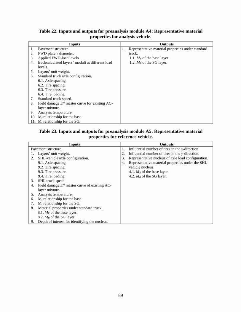
Table 22. Inputs and outputs for preanalysis module A4: Representative material

properties for analysis vehicle.

Inputs Outputs





levels.


6. Standard truck axle configuration.

6.1. Axle spacing.

6.2. Tire spacing.

6.3. Tire pressure.

6.4. Tire loading.

7. Standard truck speed.

8. Field damage E* master curve for existing AC-

layer mixture.

9. Analysis temperature.



1. Representative material properties under standard

truck.

1.1. MR of the base layer.

1.2. MR of the SG layer.

Table 23. Inputs and outputs for preanalysis module A5: Representative material

properties for reference vehicle.

Inputs Outputs

Pavement structure.


2. SHL-vehicle axle configuration.

9.1. Axle spacing.

9.2. Tire spacing.

9.3. Tire pressure.

9.4. Tire loading.

3. SHL truck speed.

4. Field damage E* master curve of existing AC-

layer mixture.




8. Material properties under standard truck.



9. Depth of interest for identifying the nucleus.

1. Influential number of tires in the x-direction.

2. Influential number of tires in the y-direction.

3. Representative nucleus of axle load configuration.

4. Representative material properties under the SHL-

vehicle nucleus.



89

Table 24. Inputs and outputs for analysis module B1: Bearing capacity.

Inputs Outputs


2. Representative nucleus of SHL-vehicle

configuration.

2.1. Axle spacing.

2.2. Tire spacing.

2.3. Tire pressure.

2.4. Tire loading.

3. SHL truck speed.


layer mixture.


6. Material properties under SHL truck.



7. Estimated τmax parameters of the SG.

1. Maximum average stress on top of the SG using

representative nucleus of SHL-vehicle

configuration.

2. qu of the SG layer.

3. FOS against general bearing capacity failure of the

SG layer and the need for mitigation strategy.

Table 25. Inputs and outputs for analysis module B2: Service limit.

Inputs Outputs



configuration.

2.1. Axle spacing.

2.2. Tire spacing.

2.3. Tire pressure.

2.4. Tire loading.

3. SHL truck speed.


layer mixture.





7. Estimated τmax parameters of the SG.


8.1. Axle spacing.

8.2. Tire spacing.

8.3. Tire pressure.

8.4. Tire loading.







13. Backcalculated moduli at different load levels.

14. Surface deflection at center of loading plate.


1. Equivalent triaxial state of stresses under nucleus

of SHL-vehicle configuration at the top of SG.

2. FOS against the localized shear failure and the

need for mitigation strategy.

3. Stress level under FWD loading and the nucleus of

SHL-vehicle configuration at the top of SG.

4. FWDequiv corresponding to the SHL using the

computed stress level.

5. Surface deflection under the nucleus of SHL-

vehicle configuration.

6. Comparison of the surface deflection under the

nucleus of SHL configuration with FWD

measurements.

7. FWDequiv corresponding to the SHL-vehicle using

computed surface displacement.

8. Need for any mitigation strategy based on the

determined FWDequiv.

90

Table 26. Inputs and outputs for analysis module B3: Service limit.

Inputs Outputs



configuration.

2.1. Axle spacing.

2.2. Tire spacing.

2.3. Tire pressure.

2.4. Tire loading.

3. SHL truck speed.


layer mixture.



6.1. MR of base layer.

6.2. MR of SG layer.

7. Estimated τmax parameters of SG.

1. Investigation of the failure development in the

sloped shoulder.

2. Need for any mitigation strategy based on slope

stability analysis.

Table 27. Inputs and outputs for analysis module B4: Buried utility.

Inputs Outputs



configuration

2.1. Axle spacing.

2.2. Tire spacing.

2.3. Tire pressure.

2.4. Tire loading.

3. SHL truck speed.


layer mixture.





1. FOS against circumferential stress failure.

2. Check for pipe ovality.

3. Check for ring buckling stress.

4. Check for wall crushing stress.

5. Need for any mitigation strategy based on buried

utility analysis.

91

Table 28. Inputs and outputs for analysis module B5: Cost allocation.

Inputs Outputs



2.1. Axle spacing.

2.2. Tire spacing.

2.3. Tire pressure.

2.4. Tire loading.



configuration.

4.1. Axle spacing.

4.2. Tire spacing.

4.3. Tire pressure.

4.4. Tire loading.

5. SHL truck speed.


layer mixture.








10. Allowable AC distress before rehabilitation at

desired reliability.

10.1. Allowable AC permanent deformation.

10.2. Allowable AC bottom-up fatigue cracking.

11. AADTT for pavement section.

12. Discount rate for present value calculation.

13. Maintenance/rehabilitation activity repair cost.

14. Performance models’ local calibration factors. 14.1. AC permanent deformation: K1, K2, K3, Br1,

Br2, Br3.

14.2. AC bottom-up fatigue cracking: K1, K2, K3,

Bf1, Bf2, Bf3.

14.3. Base permanent deformation: B1.

14.4. SG permanent deformation: B1.

15. Estimation of the number of standard trucks prior

to the pass of the SHL truck pass.

16. Estimation of E* value at the specific pavement

temperature and SHL truck operational speed.

1. Cost associated with the AC permanent

deformation.

2. Cost associated with the AC bottom-up fatigue

cracking.

3. Cost associated with the base permanent

deformation.

4. Cost associated with the SG permanent

deformation.

AADTT = annual average daily truck traffic.

5.7. SUMMARY

In this chapter, the SHL pavement analysis software package (SuperPACK) was illustrated.(9)

SuperPACK incorporates the various analysis procedures developed in this study to evaluate the

impact of SHL movements on flexible pavements. This analysis package was developed in

MATLAB as a stand-alone software with the following three main components: preanalysis

modules, analysis modules, and analysis engine. The analysis engine is called 3D-Move

ENHANCED, which is based on the formulation of 3D-Move Analysis software. The

92

enhancements included 3D surface plots for a specific pavement response at a desired depth,

layer interface conditions such as debonding or slippage, and runtime improvement.

The SuperPACK main window contains general information about the project as well as basic

information needed for 3D-Move ENHANCED analysis (e.g., layer thicknesses, material

types).(9,11) The preanalysis and analysis modules could be accessed through the SuperPACK

main window. Each of these modules has a function and a GUI specifically developed for that

module. The GUI developed for each module inputs specific information needed to execute that

module. Additionally, 3D-Move ENHANCED provides the module with necessary pavement

responses when requested. Preanalysis modules are prerequisite to proceed to analysis modules.

93

CHAPTER 6. SUMMARY AND SUGGESTED RESEARCH

6.1. SUMMARY AND VALIDATION OF DEVELOPED APPROACH

The number of SHL-vehicle movements on the Nation’s highways has grown significantly

during the past decade. Many of these superheavy components are very large in size and weight,

often requiring specialized trailers and hauling units. The SHL vehicles are mostly oversized and

exceed legal GVW, axle load, and tire load limits, warranting the need for single-trip permits.

Accordingly, a full pavement analysis is needed to ensure that the pavement is structurally

adequate to sustain the SHL movement. Consequently, the evaluation of SHL movements on

flexible pavements should be cognizant of the following important factors:

• Nonconventional SHL-vehicle axle and tire loadings and configurations.

• Slow-moving nature of SHL vehicle in relation to viscoelastic properties of AC layer.

• Role of higher magnitude stress states induced by an SHL-vehicle movement on stress-

dependent behavior of unbound materials.

• Likelihood of ultimate and localized shear failure in the influenced zone of the SG layer.

• Likelihood of excessive pavement surface deflections.

• Role of SHL-vehicle movement on the stability of a sloped pavement shoulder.

• Impact of SHL vehicle on the integrity of existing buried utilities.

• PDACs attributable to SHL-vehicle movement.

A comprehensive mechanistic-based analysis methodology seeking to address these factors

associated with SHL movement on flexible pavements was developed. In general, the

methodology consists of the following four major components:

• Ultimate failure analyses.

• Buried utility risk analysis.

• Service limit analyses.

• Cost allocation analysis.

It should be noted that mitigation strategies to attenuate the SHL vehicle–induced distresses and

damage may be needed at any stage of the evaluation process when the analysis results fail to

meet the imposed respective requirements.

One of the major tasks in this project was to estimate pavement responses (i.e., stress, strain, and

deflections) under SHL-vehicle movements. Focus is to be given to understanding the role of

governing factors such as nonstandard vehicle loading (e.g., tire configuration, tire loading, and

inflation pressure), lower SHL-vehicle speed compared to normal truck, and pavement-layer

material properties that are consistent with SHL vehicle.

95

To model SHL-vehicle movements on flexible pavements while considering the nonstandard

axle and tire configurations, a novel approach to identify element(s) of the SHL-vehicle

configuration that can be regarded as representative of the entire SHL vehicle (referred to as

nucleus) was presented. The σv distribution (or any other pavement response) under the entire

SHL-vehicle configuration can be estimated by superimposing the stresses calculated under the

nucleus, hence eliminating the need to model the entire SHL vehicle.

A critical input for the analysis of an SHL-vehicle movement when using numerical models is

the material properties of the existing pavement layers, including the SG. These properties

should appropriately represent the characteristics of the materials that exist at the time of the

SHL movement. The role of lower SHL-vehicle speed in the pavement analysis was addressed

using the E* master curve for the existing AC layer. An approach to estimate field damaged E*

master curve that considers the reduction in the AC-layer stiffness was presented. On the other

hand, the stiffness of unbound layers, such as the CAB and SG, is affected by the load-induced

stresses. The FWD backcalculated moduli for unbound materials can be viewed as a

representative stiffness in the pavement analysis when standard truck traffic is of concern.

However, in the case of an SHL vehicle, higher state of stresses, especially from overlapping of

closely spaced wheel loads, compared to those observed under a common FWD-load level, are

expected. Consequently, the FWD-based backcalculated modulus of an unbound layer may not

represent the stiffness of the layer expected under an SHL-vehicle movement. Accordingly, an

iterative approach incorporating the nonlinear stress-dependent MR relationship and the existing

state of stresses in the unbound layers was employed in this project.

The ϕ and c of the SG layer contained within the loaded influence zone (i.e., contributing

pavement SG layer) are necessary inputs for assessing the risk of instantaneous shear failure

under SHL movement of flexible pavements. These SG τmax parameters are also critical inputs

for the stability analysis of a sloped pavement shoulder under an SHL movement. In this study,

an innovative methodology to estimate in situ τmax parameters of the pavement SG layer based on

nondestructive FWD testing undertaken at multiple load levels has been developed. The validity

of the developed approach was explored using numerical simulation of FWD measurements and

FWD data collected from large-scale experiments on full-scale pavement structures as well as

APT facilities. A variety of unpaved and paved pavement structures were utilized in the

verification process.

The SHL vehicle can render a critical condition (distress modes) of instantaneous ultimate shear

failure, localized shear failure, or excessive surface deflection. To examine the risk of

instantaneous shear failure, Meyerhof’s general bearing capacity equation was used. The

distributed σv on the top of the SG induced by an SHL vehicle in comparison with the bearing

capacity of the SG layer were used to identify the possibility of ultimate shear failure in the

pavement structure. The ultimate failure analysis focused on the SG layer as it is generally the

weakest layer in pavement structures. It should be noted that a modified bearing capacity

approach was applied in the case of a sloping pavement shoulder.

Once bearing capacity investigation confirms the adequacy of pavement structure to withstand

the general shear failure, the possibility for localized shear failure needs to be evaluated. Such

analysis is conducted by computing the load-induced stress level on top of the SG layer using

96

Drucker–Prager failure criterion. A stress level closer to τmax indicates likelihood of localized

failure (yield criterion) and a need for mitigation strategies.

Although shear analyses (i.e., ultimate and localized) are viewed as a check for failure condition,

they do not provide any information regarding surface displacement (i.e., deflection) under SHL

movement. In other words, though the shear failure analyses may indicate that the pavement

structure is capable of sustaining the SHL movement without experiencing any shear failure,

excessive surface deflections resulting from SHL-vehicle loading can give rise to a rapid

deterioration of pavement structure and development of premature surface distresses (e.g.,

permanent deformation). Accordingly, the δSHL should be limited to an allowable surface

deflection. An FWDequiv to generate D0 equivalent to the surface deflection computed under the

SHL vehicle is determined and compared to FWDallow . The concept of SSR is employed to

determine FWDallow. An FWDequiv higher than the FWDallow indicates the potential accumulation

of unacceptable levels of permanent surface deformation.

SHL vehicles are usually moved under traffic control so that it is often possible to keep the SHL

vehicle away from the pavement edge and shoulder. It is recommended that the vehicle stay

away from the pavement edge, particularly on routes where there is an unpaved shoulder and/or a

deep slope. It is not always possible to keep the SHL vehicle far from the pavement edge (e.g.,

narrow lanes and/or wide SHL vehicle). Therefore, it is necessary to investigate the stability of a

sloped pavement shoulder under the SHL-vehicle movement.

In this study, the wedge method, which is a well-accepted slope stability analysis methodology in

geotechnical practice, was modified so that the stability of a sloping layered medium consisting

of pavement layers with distinct properties can be evaluated under SHL movements. Resultant

horizontal force due to the SHL vehicle is the major component of the horizontal deriving force

leading to the instability of failure wedge. The 3D-Move ENHANCED was used to compute

these horizontal stresses on the vertical face of the sliding wedge. However, the 3D-Move

ENHANCED computed stresses were modified to account for the role of the sloping shoulder

near the edge of the pavement since this software assumes that pavement layers extend laterally

to infinity. A SAF to adjust the calculated stresses in the presence of the sloped shoulder was

identified based on the results obtained from two full-scale experiments with similar pavement

structures (with and without sloped pavement shoulder). The validity of the approach was

verified using measurements obtained from a full-scale pavement structure with a sloping

shoulder.

An approach to analyze the risk against buried structures due to SHL movement on flexible

pavements was presented. The approach was based on widely accepted and available buried

utility (flexible and rigid) design procedures. For flexible pipes, a hybrid step-by-step evaluation

procedure, provided in ALA and CEPA reports, was implemented. The procedure is divided into

four general checks: (1) Assess FOS against pipe circumferential stress failure; (2) check ovality

of pipe cross section; (3) check ring buckling stress; and (4) check wall crushing stress. In the

case of rigid concrete culvert, the stability was investigated by analyzing the flexural strength,

τmax, and axial thrust in the culvert members (i.e., top slab, bottom slab, and sidewalls) in

accordance with AASHTO LRFD Bridge Design Specifications.(31)

97

Fair assessment of the induced stresses from the SHL vehicle is required to reliably analyze the

internal integrity of a buried utility. Though the existing state-of-practice methodologies provide

recommendations with respect to the load distribution, they are limited when assessing the risk

of buried utilities under an SHL-vehicle movement. Considering only a standard truck (mostly

HS20) as a live load and simulating it as a point load or over a rectangular loaded area that is

statically applied directly at the surface of unpaved roads (i.e., neglecting the AC and CAB layer)

are the significant limitations.

Therefore, the 3D-Move ENHANCED was adopted to realistically simulate pavement structure

and SHL vehicle (e.g., viscoelastic properties of the AC layer, moving load). However, the 3D-

Move ENHANCED computed stresses were modified to account for the role of buried utilities

and the soil–structure interaction. SAFs to adjust the calculated stresses in the presence of buried

utility (flexible and rigid) were also identified based on the results obtained from two full-scale

experiments with similar pavement structures (with and without buried utilities). The validity of

the approach was verified using measurements obtained from a full-scale pavement structure

with buried utilities.

After completing and satisfying the ultimate failure analyses, buried utility risk analysis, and

service limit failure analyses, the cost allocation attributable to pavement damage under an SHL

vehicle is conducted. The approach employs input information that is commonly accessible to

highway agencies and implements an ME-based analysis that considers the determination of

critical pavement responses associated with different types of pavement distresses. This cost

allocation approach estimates pavement damage costs based on vehicle axle loading and

configuration and considers the predicted pavement life reduction due to a single pass of the

evaluated SHL vehicle. With this method, different pavement distress models, pavement repair

options, and any axle configuration can be considered. The NPV of repairing costs and VMT are

also needed inputs of the process. The approach considers the current condition of the pavement

at the time of the SHL movement. Consequently, lower PDAC will be estimated for an SHL

movement occurring on a pavement section with lower remaining life (i.e., a pavement section

that has already been subjected to a percentage of its original design traffic). Factors such as

pavement temperature, SHL-vehicle operational speed, rehabilitation threshold value, and

pavement structure were found to influence PDAC.

A comprehensive user-friendly software package incorporating the 3D-Move ENHANCED

analysis engine in conjunction with the implementation of developed analysis procedures was

developed to evaluate the impact of SHL movements on flexible pavements. SuperPACK

comprises three main components: preanalysis, analysis, and analysis engine.(9) The preanalysis

modules include the respective procedures for axle grouping and nucleus of SHL analysis

vehicle, material characterization, estimation of SG τmax parameters, and representative material

properties for SHL-vehicle analysis. The analysis modules include the assessment of bearing

capacity failure, service limit, slope stability, buried utility, and cost allocation under an SHL-

vehicle movement. The 3D-Move ENHANCED analysis engine allows for the determination of

pavement responses under an SHL-vehicle loading at any depth within the pavement structure

within a reasonable amount of run time.

The analysis procedures developed to evaluate SHL movements on flexible pavement were

demonstrated using two SHL-vehicle movement cases. These two cases represented actual SHL

98

vehicles with different characteristics that consisted of fragmented and continuous axle

configurations with a GVW of 1.7 and 3.6 million lb. The findings from this exercise revealed

that the methodology was able to capture various aspects of the impact of the two SHL

movements analyzed. Similar case studies should be conducted to cover a variety of SHL-

movement scenarios (vehicles types, pavement structures and materials, existing pavement

condition, etc.). The various aspects (in situ material characterization, pavement distresses, cost

allocation, etc.) of the developed methodology should be evaluated and verified by highway

agencies using past and future permit data. Such efforts will serve as feedback to improve and

calibrate the various components of the developed methodology (e.g., estimated pavement

damage cost allocation attributable to SHL-vehicle movement).

To familiarize highway agencies’ personnel with the methodology developed and the use of

SuperPACK, training and workshop activities are needed.(9) This can be achieved by first

conducting a webinar on the overall methodology developed, assumptions, limitations, etc.,

followed by hands-on training on the use of SuperPACK, which includes preanalysis, analysis,

and postprocessing of the results.

6.2. SUGGESTED RESEARCH

The comprehensive mechanistic-based analysis methodology developed addressed several

factors governing the assessment of the impact of SHL movement on flexible pavements. The

methodology was based on well-accepted and available analysis and evaluation procedures.

Simplified yet reasonable assumptions such as those related to the type of tire, characterization

of the tire–pavement interaction stresses, and pavement material characterization were utilized in

the analysis procedures.

The following are suggested future developments and enhancements of the developed

methodology:

• Constant tire pressure with a circular tire–pavement contact area was utilized. However,

3D-Move ENHANCED is capable of handling nonuniform contact pressure of any shape

(not necessarily circular), including stress distributions from wide-base tires that can be

an attractive option for SHL vehicles. Such cases can be readily investigated using the

methodology developed.

• The SHL vehicle was assumed moving under constant speed conditions. However, 3D-

Move ENHANCED allows for modeling vehicle loading under braking and turning

conditions as well as sloping pavement grade (uphill or downhill). Thus, the impact of

tire-induced shear stresses exerted on the pavement surface under such circumstances can

be addressed and incorporated in the developed methodology.

• The backcalculation analysis to determine the moduli of the existing pavement layers

should be undertaken independently from the developed analysis procedures. A potential

improvement is the incorporation of the backcalculation process as a part of the

developed methodology.

99

• The estimate of in situ τmax parameters of the pavement SG layer is based on

nondestructive FWD testing undertaken at multiple load levels. The range of the FWD-

load levels should result in a state of stresses in the pavement structure that are consistent

with the anticipated stresses induced by an SHL-vehicle movement. A practical

consideration is the development of a procedure to identify the desired FWD-load levels

as part of SHL-movement investigation/analysis.

• SAFs were determined for sloped pavement shoulders and buried utilities based on test

results from three full-scale pavement experiments. Further investigation by conducting

complementary experiments and additional numerical analyses is recommended to extend

the findings to other case scenarios. Such investigations should consider, in the case of

sloped pavement shoulders, various scenarios of flexible pavement structures and

materials, slope angles, distance of the surface load from the edge of the slope, etc. In the

case of buried utilities, the investigation should also consider various scenarios of depth

of cover, buried utility dimensions and characteristics, interaction between adjacent

utilities, etc.

• SuperPACK was established in MATLAB as a stand-alone software program to

implement the various aspects of the developed methodology.(9) A Web-based next

generation of the software can be developed so that authorities in highway agencies and

engineers dealing with SHL movement can readily use SuperPACK online. The new

version should incorporate enhancements and improvements, such as the ones previously

suggested, to the developed methodology. The analysis associated with the mitigation

strategies can also be integrated within the new version of the SuperPACK framework.

• The overall procedures developed in this study for failure investigation under an SHL-

vehicle movement are general in nature, and they require the estimation of select critical

pavement responses. In cases involving rigid pavements, appropriate techniques to

estimate needed responses can be potentially used to investigate applicable failure modes.

Such an investigation should account for factors specifically related to rigid pavements

(e.g., longitudinal and transverse joints characteristics, curling and warping conditions).

100

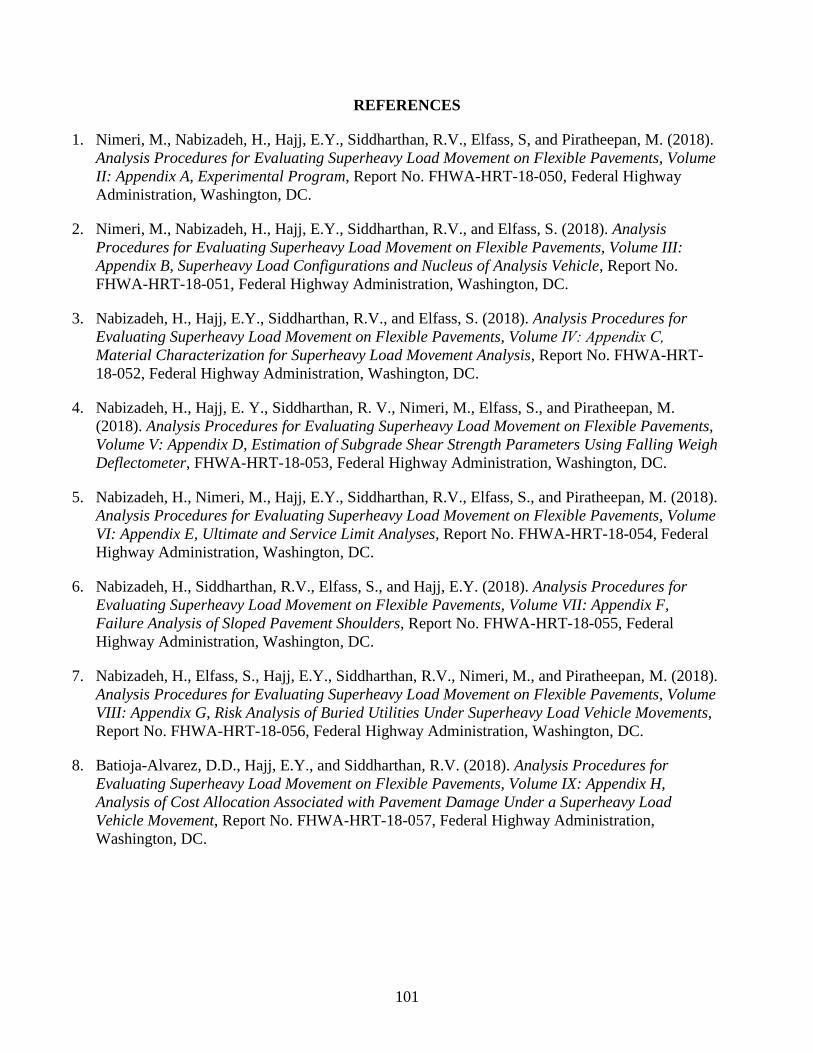
REFERENCES

1. Nimeri, M., Nabizadeh, H., Hajj, E.Y., Siddharthan, R.V., Elfass, S, and Piratheepan, M. (2018).

Analysis Procedures for Evaluating Superheavy Load Movement on Flexible Pavements, Volume

II: Appendix A, Experimental Program, Report No. FHWA-HRT-18-050, Federal Highway

Administration, Washington, DC.

2. Nimeri, M., Nabizadeh, H., Hajj, E.Y., Siddharthan, R.V., and Elfass, S. (2018). Analysis

Procedures for Evaluating Superheavy Load Movement on Flexible Pavements, Volume III:

Appendix B, Superheavy Load Configurations and Nucleus of Analysis Vehicle, Report No.

FHWA-HRT-18-051, Federal Highway Administration, Washington, DC.

3. Nabizadeh, H., Hajj, E.Y., Siddharthan, R.V., and Elfass, S. (2018). Analysis Procedures for

Evaluating Superheavy Load Movement on Flexible Pavements, Volume Ⅳ: Appendix C,

Material Characterization for Superheavy Load Movement Analysis, Report No. FHWA-HRT-

18-052, Federal Highway Administration, Washington, DC.

4. Nabizadeh, H., Hajj, E. Y., Siddharthan, R. V., Nimeri, M., Elfass, S., and Piratheepan, M.

(2018). Analysis Procedures for Evaluating Superheavy Load Movement on Flexible Pavements,

Volume V: Appendix D, Estimation of Subgrade Shear Strength Parameters Using Falling Weigh

Deflectometer, FHWA-HRT-18-053, Federal Highway Administration, Washington, DC.

5. Nabizadeh, H., Nimeri, M., Hajj, E.Y., Siddharthan, R.V., Elfass, S., and Piratheepan, M. (2018).


VI: Appendix E, Ultimate and Service Limit Analyses, Report No. FHWA-HRT-18-054, Federal

Highway Administration, Washington, DC.

6. Nabizadeh, H., Siddharthan, R.V., Elfass, S., and Hajj, E.Y. (2018). Analysis Procedures for

Evaluating Superheavy Load Movement on Flexible Pavements, Volume VII: Appendix F,

Failure Analysis of Sloped Pavement Shoulders, Report No. FHWA-HRT-18-055, Federal


7. Nabizadeh, H., Elfass, S., Hajj, E.Y., Siddharthan, R.V., Nimeri, M., and Piratheepan, M. (2018).


VIII: Appendix G, Risk Analysis of Buried Utilities Under Superheavy Load Vehicle Movements,

Report No. FHWA-HRT-18-056, Federal Highway Administration, Washington, DC.

8. Batioja-Alvarez, D.D., Hajj, E.Y., and Siddharthan, R.V. (2018). Analysis Procedures for

Evaluating Superheavy Load Movement on Flexible Pavements, Volume IX: Appendix H,

Analysis of Cost Allocation Associated with Pavement Damage Under a Superheavy Load

Vehicle Movement, Report No. FHWA-HRT-18-057, Federal Highway Administration,

Washington, DC.

101

9. Kazemi, S.F., Nabizadeh, H., Nimeri, M., Batioja-Alvarez, D.D., Hajj, E.Y., Siddharthan, R.V.,

and Hand, A.J.T. (2018). Analysis Procedures for Evaluating Superheavy Load Movement on

Flexible Pavements, Volume X: Appendix I, Analysis Package for Superheavy Load Vehicle

Movement on Flexible Pavement (SuperPACK), Report No. FHWA-HRT-18-058, Federal


10. National Cooperative Highway Research Program. (2008). State Highway Cost Allocation

Studies, NCHRP Synthesis 378, National Cooperative Highway Research Program,

Transportation Research Board, National Research Council, Washington, DC.

11. Seyed-Farzan, K. (2018). “3D-FAST: Three-Dimensional Fourier Analysis of Pavement

Structures Under Transient Loading.” (dissertation) Department of Civil and Environmental

Engineering, University of Nevada, Reno, NV.

12. 3D-Move Analysis software v2.1. (2013). Developed by University of Nevada, Reno, NV.

Available online: http://www.arc.unr.edu/Software.html#3DMove, last accessed September

19, 2017.

13. Rada, G.R., Nazarian, S., Visintine, B.A., Siddharthan, R., and Thyagarajan, S. (2016).

Pavement Structural Evaluation at the Network Level, Report No. FHWA-HRT-15-074, Federal


14. National Cooperative Highway Research Program. (2004). Guide for Mechanistic–Empirical

Design of New and Rehabilitated Pavement Structures, Transportation Research Board,

Washington, DC.

15. AASHTO T 319. (2015). Standard Method of Test for Quantitative Extraction and Recovery of

Asphalt Binder From Asphalt Mixtures, American Association of State Highway and

Transportation Officials, Washington, DC.

16. AASHTO T 315-12. (2016). Standard Method of Test for Determining the Rheological

Properties of Asphalt Binder Using a Dynamic Shear Rheometer (DSR), American Association

of State Highway and Transportation Officials, Washington, DC.

17. AASHTO T 378-17. (2017). Standard Method of Test for Determining the Dynamic Modulus

and Flow Number for Asphalt Mixtures Using the Asphalt Mixture Performance Tester (AMPT),

American Association of State Highway and Transportation Officials, Washington, DC.

18. AASHTO T 166-16. (2016). Standard Method of Test for Bulk Specific Gravity (Gmb) of

Compacted Hot Mix Asphalt (HMA) Using Saturated Surface-Dry Specimens, American

Association of State Highway and Transportation Officials, Washington, DC.

19. AASHTO T 209-12. (Revised 2016). Standard Method of Test for Theoretical Maximum Specific

Gravity (Gmm) and Density of Hot-Mix Asphalt, American Association of State Highway and

Transportation Officials, Washington, DC.

102

http://www.arc.unr.edu/Software.html#3DMove

20. AASHTO T 30-15. (2015). Standard Method of Test for Mechanical Analysis of Extracted

Aggregate, American Association of State Highway and Transportation Officials, Washington,

DC.

21. Groeger, J. L., Rada, G. R., and Lopez, A. (2003). “AASHTO T 307-Background and

Discussion,” Resilient Modulus Testing for Pavement Components, Report No. ASTM STP 1437, ASTM, West Conshohocken, PA.

22. AASHTO T 307-99. (2017). Standard Method of Test for Determining the Resilient Modulus of

Soils and Aggregate Materials, American Association of State Highway and Transportation

Officials, Washington, DC.

23. Nabizadeh, H., Hajj, E.Y., Siddharthan, R., Elfass, S., and Nimeri, N. (2017). “Application of Falling Weight Deflectometer for the Estimation of In Situ Shear Strength Parameters of

Subgrade Layer.” Bearing Capacity of Roads, Railways, and Airfields, pp. 743–749, Taylor &

Francis Group, Milton Park, Didcot, United Kingdom.

24. Nabizadeh, H., Hajj, E.Y., Siddharthan, R., Elfass, S., and Sebaaly, P.E. (2016). “Estimation of In Situ Shear Strength Parameters for Subgrade Layer Using Non-destructive Testing.” The

Roles of Accelerated Pavement Testing in Pavement Sustainability, pp. 525–538, Springer,

Cham, Switzerland.

25. Kondner, R.L. (1963). “Hyperbolic Stress-Strain Response: Cohesive Soils.” Journal of the Soil

Mechanics and Foundations Division, 89(1), pp. 115–144, American Society of Civil Engineers,

Reston, VA.

26. Duncan, J.M. and Chang, C.Y. (1970). “Nonlinear Analysis of Stress and Strain in Soils.” Journal of the Soil Mechanics and Foundations Division, 96(5), pp. 1,629–1,653, American

Society of Civil Engineers, Reston, VA.

27. Das, B.M. and Sobhan, K. (2014). Principles of Geotechnical Engineering, Cengage Learning,

Stamford, CT.

28. U.S. Army Corps of Engineers. (2003). Slope Stability, Department of the Army, Washington,

DC.

29. American Lifelines Alliance. (2001). Guidelines for the Design of Buried Steel Pipe, American


30. Warman, D.J., Hart, J.D., and Francini, R.B. (2009). Development of a Pipeline Surface Loading

Screening Process and Assessment of Surface Load Dispersing Methods, Report No. 05-44R1,

Canadian Energy Pipeline Association, Worthington, OH.

31. AASHTO. (2012). AASHTO LRFD Bridge Construction Specifications, Sixth Edition, American

Association of State Highway and Transportation Officials, Washington, DC.

32. Drucker, D.C. and Prager, W. (1952). “Soil Mechanics and Plastic Analysis or Limit Design.” Quarterly of Applied Mathematics, 10(2), pp. 157–165, Brown University, Providence, RI.

103

33. Chow, L.C., Mishra, D., and Tutumluer, E. (2014). “Framework for Development of an

Improved Unbound Aggregate Base Rutting Model for Mechanistic–Empirical Pavement

Design.” Transportation Research Record, 2401, pp. 11–21, Transportation Research Board,

Washington, DC.

34. Kazmee, H. and Tutumluer, E. (2015). Evaluation of Aggregate Subgrade Materials Used as

Pavement Subgrade/Granular Subbase, Report No. FHWA-ICT-15-013, Federal Highway


35. Seyhan, U. and Tutumluer, E. (2002). “Anisotropic Modular Ratios as Unbound Aggregate Performance Indicators.” Journal of Materials in Civil Engineering, 14(5), pp. 409–416,

American Society of Civil Engineers, Reston, VA.

36. Tutumluer, E., Kim, I.T., and Santoni, R.L. (2004). “Modulus Anisotropy and Shear Stability of

Geofiber-Stabilized Sands.” Transportation Research Record, 1874, pp. 125–135,

Transportation Research Board, Washington, DC.

37. Tirado, C., Carrasco, C., Mares, J.M., Gharaibeh, N., Nazarian, S., and Bendana, J. (2010).

“Process to Estimate Permit Costs for Movement of Heavy Trucks on Flexible Pavements,” Transportation Research Record, 2154, pp. 187–196, Transportation Research Board,

Washington, DC.

38. Raad, L. and Figueroa, J.L. (1980). “Load Response of Transportation Support Systems.”

Journal of Transportation Engineering, 106(1), pp. 111–128, American Society of Civil

Engineers, Reston, VA.

39. BAKFAA V2.0. (2012). Backcalculation software, Federal Aviation Administration,

Washington, DC.

40. Rohde, G.T. and Scullion, T. (1990). MODULUS 4.0: Expansion and Validation of the

MODULUS Backcalculation System, Report No. FHWA/TX-91/1123-3, Texas Transportation

Institute, College Station, TX.

41. Kenis, W.J. (1978). Predictive Design Procedures, VESYS User’s Manual: An Interim Design

Method for Flexible Pavements Using the VESYS Structural Subsystem, Report No. FHWA-RD-

77-154, Pavement System Group, Structures and Applied Mechanics Division, Federal Highway


42. DeJong, D.L., Pentz, M.G.F., and Korswagen, A.R. (1973). Computer Program BISAR,

Koninklijke/Shell-Laboratorium, Amsterdam, Netherlands.

43. Huang, Y.H. (2004). Pavement Analysis and Design, Pearson Education, Cranbury, NJ.

44. Harichandran, R.S., Yeh, M.S., and Baladi, G.Y. (1990). “MICH-PAVE: A Nonlinear Finite

Element Program for Analysis of Flexible Pavements.” Transportation Research Record, 1286,

pp. 123–131, Transportation Research Board, Washington, DC.

104

45. Siddharthan, R.V., Yao, J., and Sebaaly, P.E. (1998). “Pavement Strain From Moving Dynamic 3D Load Distribution.” Journal of Transportation Engineering, 124(6), pp. 557–566, American


46. Maina, J.W., De Beer, M., and Matsui, K. (2007). “Effects of Layer Interface Slip on the Response and Performance of Elastic Multi-Layered Flexible Airport Pavement Systems.” International Conference on Maintenance and Rehabilitation of Pavements and Technological

Control (MAIREPAV5), Fifth Proceedings, pp. 145–150, University of Iowa, Iowa City, IA.

105

HRDI-20/10-18(WEB)E

Documents

of Transportallon Errata...Volume Ⅰ is the final report, and Volume Ⅱthrough Volume Ⅹconsist of Appendix A through Appendix Ⅰ. Any reference to a volume in this series will