Offshoring and Unemployment: The Role of Search Frictions and Labor Mobility *

Devashish Mitra Priya Ranjan†

Syracuse University University of California – Irvine

February, 2009

Abstract In a two-sector, general-equilibrium model with labor-market search frictions, we find that wage increases and sectoral unemployment decreases upon offshoring in the presence of perfect intersectoral labor mobility. If, as a result, labor moves to the sector with the lower (or equal) vacancy costs, there is an unambiguous decrease in economywide unemployment. With imperfect intersectoral labor mobility, unemployment in the offshoring sector can rise, with an unambiguous unemployment reduction in the non-offshoring sector. Imperfect labor mobility can result in a mixed equilbrium in which only some firms in the industry offshore, with unemployment in this sector rising. Keywords: Trade, Offshoring, Search, Unemployment JEL Classification Codes: F11, F16, J64

* We thank seminar participants at Carleton University, Drexel University, Federal Reserve Bank of St.Louis, Georgia Tech, the Indian School of Business (Hyderabad), KU Leuven, Oregon State University, University of Virginia and the World Bank, and conference participants at the 2007 Globalization Conference at Kobe University in Japan, the 2008 AEA meetings in New Orleans, the Centro Studi Luca d'Agliano Conference on Outsourcing and Immigration held in Fondazione Agnelli in Turin (Italy), the Midwest International Trade Conference in Minneapolis (Spring, 2007), and the NBER Spring 2007 International Trade and Investment group meeting for useful comments and discussions. We are indebted to Pol Antras (our discussant at the 2008 AEA meetings), Jonathan Eaton (the Editor) and two anonymous referees for very detailed and useful comments on earlier versions. The standard disclaimer applies. † Corresponding author: Department of Economics, University of California-Irvine, Irvine, CA 92697, Email: pranjan@uci.edu , Ph: (949) 824-1926, FAX: (949) 824-2192.

1 Introduction

"O¤shoring" is the sourcing of inputs (goods and services) from foreign countries. When production of these

inputs moves to foreign countries, the fear at home is that jobs will be lost and unemployment will rise.

In the recent past, this has become an important political issue. The remarks by Greg Mankiw, when he

was Head of the President�s Council of Economic Advisers, that "outsourcing is just a new way of doing

international trade" and is "a good thing" came under sharp attack from prominent politicians from both

sides of the aisle. Recent estimates by Forrester Research of job losses due to o¤shoring equaling a total of

3.3 million white collar jobs by 2015 and the prediction by Deloitte Research of the outsourcing of 2 million

�nancial sector jobs by the year 2009 have drawn a lot of attention from politicians and journalists (Drezner,

2004), even though these job losses are only a small fraction of the total number unemployed, especially when

we take into account the fact that these losses will be spread over many years.1 Furthermore, statements

by IT executives have added fuel to this �re. One such statement was made by an IBM executive who

said "[Globalization] means shifting a lot of jobs, opening a lot of locations in places we had never dreamt

of before, going where there is low-cost labor, low-cost competition, shifting jobs o¤shore", while another

statement was made by Hewlett-Packard CEO Carly Fiorina in her testimony before Congress that "there

is no job that is America�s God-given right anymore" (Drezner, 2004). The alarming estimates by Bardhan

and Kroll (2003) and McKinsey (2005) that 11 percent of our jobs are potentially at risk of being o¤shored

have provided anti-o¤shoring politicians with more ammunition for their position on this issue.

While the relation between o¤shoring and unemployment has been an important issue for politicians,

the media and the public, there has hardly been any careful theoretical analysis of this relationship by

economists. In this paper, in order to study the impact of o¤shoring on sectoral and economywide rates of

unemployment, we construct a two-sector, general-equilibrium model in which unemployment is caused by

search frictions a la Pissarides (2000).2 There is a single factor of production, labor. Firms in one sector,

called sector Z; use labor to produce two inputs which are then assembled into output. The production of

one of these inputs (production input) can be o¤shored, but the other input (headquarter services) must be

produced using domestic labor only. There is another sector, X; that uses only domestic labor to produce

its output. Goods Z and X are combined to produce the consumption good C.

1The average number of gross job losses per week in the US is about 500,000 (Blinder, 2006). Also see Bhagwati, Panagariya

and Srinivasan (2004) on the plausibility and magnitudes of available estimates of the unemployment e¤ects of o¤shoring.

2For a comprehensive survey of the search-theoretic literature on unemployment, see Rogerson, Shimer and Wright (2005).

1

An important result of this paper is that in the presence of perfect intersectoral labor mobility, o¤shoring

leads to wage increases and unemployment reductions in both sectors. The very basic intuition is that

there will be gains from international trade which in this case takes the form of o¤shoring. In a truly

single-factor model, this would mean that this factor of production gains from trade, and that explains

why, when labor is intersectorally perfectly mobile, real wage increases and unemployment declines. When

there are impediments to intersectoral labor mobility, it is possible for unemployment to increase in the Z

sector (o¤shoring sector), however, unemployment in the X sector must decrease. The very basic intuition

is that with impediments to labor mobility, we are e¤ectively moving away from a one-sector model. Thus,

even with overall gains from trade, we can have winners and losers. When labor is totally immobile across

sectors, in our set up we truly have a two-factor model, and both factors need not necessarily be winners

from o¤shoring (trade). Since o¤shoring is similar to a technological improvement in in the Z sector, the

relative supply of Z increases and its relative price falls as a result (the relative price of X rises). Given that

X-sector labor has to win from trade due to the positive relative price e¤ect in its favor, the only possible

loser, if at all there is one, is Z-sector labor.

Moving from the very basic to more detailed intuition, o¤shoring reduces the cost of production and hence

the relative price of good Z, since one of the inputs is o¤shored and is cheaper. The resulting increase in the

relative price of the non-o¤shoring sector X leads to greater job creation and hence reduced unemployment

there. The impact of o¤shoring on Z-sector unemployment depends on the relative strengths of two mutually

opposing forces, namely the decrease in the relative price of Z, and the increase in the marginal product

of workers engaged in headquarter activities there (each such worker now working with more production

input, since it is cheaper). In the presence of perfect labor mobility, the no arbitrage condition ensures that

the second e¤ect dominates and that increases job creation and wages in sector Z. Otherwise, labor would

keep �owing out of this sector. Even though o¤shoring of the production input destroys the jobs of workers

engaged in the production of this input in the Z sector, additional Z-sector headquarter jobs and X-sector

jobs, in excess of the production jobs o¤shored, are created.

In the imperfect labor mobility case, it is possible in the Z sector for the negative relative price e¤ect

to dominate the positive productivity e¤ect. Among many factors, the net e¤ect will also depend on the

per-unit cost post o¤shoring of the input that has been o¤shored. If this cost is low enough, we get complete

o¤shoring of the production of the o¤shorable input. The reason is that in this case the domestic demand for

good Z is very high. Therefore, all domestic employment in that sector has to be used in headquarter activity

to be combined with a large amount of the cheap imported input (whose production has been o¤shored). For

2

low enough cost of o¤shoring, we get an increase in wage and a reduction in unemployment in the Z sector,

as a very large amount of the imported input per unit of headquarter labor yields a very high marginal

product of domestic headquarter labor in that sector.

At relatively high costs of the o¤shored input (even though lower than the autarky cost of producing

that input at home), we get incomplete o¤shoring (mixed equilibrium) where some �rms o¤shore and others

do not. Wages in the Z sector are lower and unemployment there higher as compared to autarky. The

intuition here is as follows: At these levels of o¤shoring costs, the price of Z is not low enough for the

quantity demanded to call for complete o¤shoring. Firms in the incomplete o¤shoring case are indi¤erent

in the o¤shoring equilibrium between o¤shoring and not o¤shoring. This means that the domestic cost of

producing the o¤shorable input gets equalized to the cost of the imported o¤shored input, which brings the

domestic wage down and the unemployment up relative to autarky. Incomplete o¤shoring makes domestic

labor and the imported input perfect substitutes at the margin. This channel of competitive pressure on

the domestic price of labor goes away when there is complete o¤shoring. Thus, the relationship between

o¤shoring costs and sectoral unemployment (and wage) in sector Z is non-monotonic in the imperfect mobility

case.

The impact of o¤shoring on overall economywide unemployment (even though sectoral unemployment

rates fall in both sectors) also depends on how the structure or the composition of the economy changes.

The exception is the case where, in addition to perfect intersectoral labor mobility, the search costs and

hence unemployment rates (and the reduction in them upon o¤shoring) in the two sectors are identical and

equal to the overall economywide unemployment rate (and its reduction). Now maintaning perfect labor

mobility, when search costs (and therefore equilibrium unemployment rates) are made unequal across the

two sectors, whether the overall unemployment rate goes up or down will also depend on which sector�s

share in the economy�s labor force expands. This is true even though we have unambiguously falling sectoral

unemployment rates. Since the employment share of the o¤shoring sector (sector Z) falls upon o¤shoring

for most of the parameter space, aggregate unemployment for those parameter values will fall if this sector

has the higher search cost (higher unemployment rate). Obviously, there is ambiguity in the opposite case,

where the search cost is smaller in the Z sector.

Our theoretical results are consistent with the empirical results of Amiti and Wei (2005a, b) for the

US and the UK. They �nd no support for the �anxiety� of �massive job losses� associated with o¤shore

3

outsourcing from developed to developing countries.3 Using data on 78 sectors in the UK for the period

1992-2001, they �nd no evidence in support of a negative relationship between employment and outsourcing.

In fact, in many of their speci�cations the relationship is positive. In the US case, they �nd a very small,

negative e¤ect of o¤shoring on employment if the economy is decomposed into 450 narrowly de�ned sectors

which disappears when one looks at more broadly de�ned 96 sectors. Alongside this result, they also �nd a

positive relationship between o¤shoring and productivity. These results are consistent with opposing e¤ects

on employment (and unemployment) created by o¤shoring. In this context , Amiti and Wei (2005a) write:

�On the one hand, every job lost is a job lost. On the other hand, �rms that have outsourced may become

more e¢ cient and expand employment in other lines of work. If �rms relocate their relatively ine¢ cient

parts of the production process to another country, where they can be produced more cheaply, they can

expand their output in production for which they have comparative advantage. These productivity bene�ts

can translate into lower prices generating further demand and hence create more jobs. This job creation

e¤ect could in principle o¤set job losses due to outsourcing.�This intuition is consistent with the channels in

our model and the reason for obtaining a result that shows a reduction in sectoral and overall unemployment

as a result of o¤shoring.

A discussion of the related theoretical literature is useful here, as it puts in perspective the need for

our analysis. While the relationship between o¤shoring and unemployment has not been analytically stud-

ied before by economists, there is now a vast literature on o¤shoring and outsourcing.4 All the models in

that literature, following the tradition in standard trade theory, assume full employment. In spite of this

assumption in the existing literature, it is important to note that our results are similar in spirit to those

in an important recent contribution by Grossman and Rossi-Hansberg (2008) where they model o¤shoring

as "trading in tasks" and show that even factors of production whose tasks are o¤shored can bene�t from

o¤shoring due to its productivity enhancing e¤ect. Our paper is also closely related to the fragmentation

literature which analyzes the economic e¤ects of breaking down the production process into di¤erent com-

ponents, some of which can be moved abroad.5 In this literature, the possibility of fragmentation leading to

the equivalent of technological improvement in an industry has been shown.6

3The o¤shoring variable they use, which they call o¤shoring intensity, is de�ned as the share of imported inputs (material

or service) as a proportion of total nonenergy inputs used by the industry.

4See Helpman (2006) for a review of this literature.

5See for instance Arndt (1997), Jones and Kierzkowski (1990 and 2001) and Deardor¤ (2001a and b).

6See for instance Jones and Kierzkowski (2001).

4

Also closely related to our work is a very recent working paper by Davidson, Matusz and Shevchenko

(2006) that uses a model of job search to study the impact of o¤shoring of high-tech jobs on low and high-

skilled workers�wages, and on overall welfare. Another paper looking at the impact of o¤shoring on the labor

market is Karabay and McLaren (2006) who study the e¤ects of free trade and o¤shore outsourcing on wage

volatility and worker welfare in a model where risk sharing takes place through employment relationships.

Bhagwati, Panagariya and Srinivasan (2004) also analyze in detail the welfare and wage e¤ects of o¤shoring.

It is also important to note that there does exist a literature on the relationship between trade and search

induced unemployment (e.g. Davidson and Matusz (2004), Moore and Ranjan (2005), Helpman and Itskhoki

(2007)). The main focus of this literature, as discussed in Davidson and Matusz, has been the role of e¢ ciency

in job search, the rate of job destruction and the rate of job turnover in the determination of comparative

advantage.7 Using an imperfectly competitive set up, Helpman and Itskhoki look at how gains from trade

and comparative advantage depend on labor market rigidities as captured by search and �ring costs and

unemployment bene�ts, and how labor-market policies in a country a¤ect its trading partner. Moore and

Ranjan, whose focus is quite di¤erent from the rest of the literature on trade and search unemployment,

show that the impact of skill-biased technological change on unemployment can be quite di¤erent from that

of globalization. None of these models deals with o¤shoring.

2 The Model

2.1 Preferences

All agents share the identical lifetime utility function from consumption given byZ 1

t

exp�r(s�t) C(s)ds; (1)

where C is consumption, r is the discount rate, and s is a time index. Asset markets are complete. The

form of the utility function implies that the risk-free interest rate, in terms of consumption, equals r.

Each worker has one unit of labor to devote to market activities at every instant of time. The total size

of the workforce is L: The �nal consumption good C is produced under CRS using two goods Z and X as

7See also the in�uential and well cited paper by Davidson, Martin and Matusz (1999) for a careful analysis of these relation-

ships under very general conditions.

5

inputs (or equivalently can be considered to be a composite basket of these two goods) as follows:

C = F (Z;X) (2)

We choose the �nal consumption good C as numeraire. Let Pz and Px be the prices of Z and X; respectively.

Since the price of C = 1; we get

1 = g(Pz; Px) (3)

where g is increasing in both Pz and Px: Therefore, an increase in Pz implies a decrease in Px: Also, (2)

implies that the relative demand for Z is given by�Z

X

�d= f(

PzPx); f 0 < 0 (4)

In addition to the utility from consumption, workers also have idiosyncratic preferences for working in

a particular sector which is captured by a per-period non-pecuniary utility (or disutility) to individual-j of

"ji from being part of the labor force in sector-i:8 This can arise from individual-speci�c preference for the

region in which this industry is located or from the individual speci�c costs of updating one�s human capital

that may di¤er across sectors.9 De�ne 'j � "jz� "jx: The distribution function of ' is denoted by G('): This

is our way of introducing mobility cost in the model. If 'j > 0; then 'j is the cost to worker j of moving

from sector Z to sector X: Similarly, if 'j < 0; it is costly for worker j to move from sector X to sector Z:

'j = 0; 8j, will capture perfect mobility.

2.2 Goods and labor markets

Production of good X is undertaken by perfectly competitive �rms. To produce one unit of X a �rm needs

to hire one unit of labor.

Z is also produced by competitive �rms, but using a slightly more sophisticated technology involving two

separate stages which are then combined. The production function for Z is given as follows.

Z = (�m�h + (1� �)m

�p)

1� (5)

8 In the case of an extra utility, "ji > 0; while in the case of an extra disutility, "ji < 0:

9As a simplifying assumption, one can assume full obsolescence or depreciation of one�s human capital or skills each period.

In order to work or search each period in a particular sector, an individual has to incur costs each period to acquire the updated

sector-speci�c human capital. These costs can be assumed to be indivudual- and sector-speci�c.

6

wheremh is the labor input into certain core activities (say headquarter services) which have to remain within

the home country and mp is the labor input for production activities which can potentially be o¤shored.

� = 11�� is the elasticity of substiution between headquarter services and production services.

If we denote the total amount of labor employed by a �rm by N; then we have

N = mh +mp (6)

To produce either X or Z, a �rm needs to open job vacancies and hire workers. The cost of vacancy in

terms of the numeraire good is ci in sector i = X;Z.10 Let Li be the total number of workers who look for

a job in sector i: Any job in either sector can be hit with an idiosyncratic shock with probability � and be

destroyed. De�ne �i = viuias the measure of market tightness in sector i; where viLi is the total number

of vacancies in sector i and uiLi is the number of unemployed workers searching for jobs in sector i. The

probability of a vacancy �lled is q(�i) =m(vi;ui)

viwhere m(vi; ui) is a constant returns to scale matching

function. Since m(vi; ui) is constant returns to scale, q0(�i) < 0: The probability of an unemployed worker

�nding a job is m(vi;ui)ui

= �iq(�i) which is increasing in �i:

2.3 Pro�t maximization by �rms

Denote the number of vacancies posted by a �rm in the Z sector by V: Assuming that each �rm is large enough

to employ and hire enough workers to resolve the uncertainty of job in�ows and out�ows, the dynamics of

employment for a �rm is:

N(t) = q(�z(t))V (t)� �N(t) (7)

The wage for each worker is determined by a process of Nash bargaining with the �rm separately which

(along with alternative modes of bargaining, including multilateral bargaining) is discussed later. While

deciding on how many vacancies to open up the �rm correctly anticipates this wage. E¤ectively, the �rm

solves a two stage problem where in stage 1 it chooses vacancies and in stage 2 it enters into bargaining

with workers to determine wages.11 Therefore, the pro�t maximization problem for an individual �rm can

10The robustness of our results to alternatively de�ning and �xing vacancy costs in terms of good Z or in terms of labor is

discussed in the penultimate section of this paper.

11As shown by Stole and Zwiebel (1996), the subgame perfect equilibrium of this type of set up can possibly involve a choice

of employment greater than what a wage taking �rm would do. This is because by choosing higher employment in stage 1 a �rm

can lower the marginal product of a worker and thus reduce the wage it has to pay in the second stage. As we will see shortly

for the autarky case (and later for the o¤shoring case), the value of marginal product of labor in our set up will be constant for

7

be written as

MaxV (s);mh(s);mp(s)

Z 1

t

e�r(s�t) fPz(s)Z(s)� wz(s)N(s)� czV (s)g ds (8)

The �rm maximizes (8) subject to (5), (6), and (7). We provide details of the �rm�s maximization exercise

in the appendix. Since we are going to study only the steady state in this paper, we suppress the time

index hereafter. The steady-state is characterized by:

N(t) = 0: From the �rst-order conditions of the �rm�s

maximization problem, the optimal mix of headquarter and production labor is given by

mh

mp=

��

1� �

��(9)

which in turn makes the output e¤ectively linear in the total employment of the �rm as follows:

Z = � 0N (10)

where � 0 � [�� + (1� �)�] 1��1 :

The key equation from the �rm�s optimal choice of vacancy, derived in the appendix, is given by

� 0Pz � wz(r + �)

=czq(�z)

(11)

The expression on the left-hand side is the marginal bene�t from creating a job which equals the present

value of the stream of the value of marginal product net of wage of an extra worker after factoring in the

probability of job separation each period. The expression on the right-hand side is the cost of creating a

job which equals the cost of posting a vacancy, cz; multiplied by the average duration of a vacancy, 1q(�z)

.

The left hand side of (11) is also the asset value of an extra job for a �rm which will be useful in the wage

determination below. An alternative way to write (11) is

� 0Pz = wz +(r + �)czq(�z)

(12)

That is, the value of marginal product of a worker is equal to the marginal cost of hiring a worker. This

is the modi�ed pricing equation in the presence of search frictions where in addition to the standard wage

cost, expected search cost is added to compute the marginal cost of hiring a worker. This is also known as

the job creation condition in the literature.

a given Pz , and therefore, a �rm has no such strategic motive. Hence, the second stage wage is e¤ectively independent of the

�rst stage employment choice (see Cahuc and Wasmer (2001) for a formal proof).

8

Since the X sector uses one unit of labor to produce one unit of output, the marginal revenue product

of labor in the X sector simply equals Px, and therefore, the pro�t maximization by �rms in the X sector

yields the following analogue of (12)

Px = wx +(r + �)cxq(�x)

(13)

2.4 Determination of Unemployment

Denoting the rate of unemployment in sector-i by ui; in steady-state the �ow into unemployment must equal

the �ow out of unemployment:

�(1� ui) = �iq(�i)ui; i = x; z

The above implies

ui =�

� + �iq(�i); i = x; z (14)

The above is the standard Beveridge curve in Pissarides type search models where the rate of unemployment

is positively related to the probability of job destruction, �; and negatively related to the degree market

tightness �i:

2.5 Wage Determination

Wage is determined for each worker through a process of Nash bargaining with his/her employer. Workers

bargain individually and simultaneously with the �rm.12 Rotemberg (2006) justi�es this assumption by

viewing it as a situation where each worker bargains with a separate representative of the �rm. Thus each

worker and the representative that he bargains with assume at the time of bargaining that the �rm will

reach a set of agreements with the other workers that leads these to remain employed.

Denoting the unemployment bene�t in terms of the �nal good by b, it is shown in the appendix that the

expression for wage is the same as in a standard Pissarides model and is given by

wi = b+�ci1� � [�i +

r + �

q(�i)]; i = x; z (15)

where � represents the bargaining power (weight) of the worker relative to the employer (See appendix). The

above wage equation along with the (12) and (14) derived earlier are the three key equations determining

wz; �z; and uz for a given Pz: For the X sector the three key equations are (13), (14), and (15).

12As explained in the previous footnote, under CRS to labor, the bargaining outcome is the same as in Stole and Zweibel

(1996), the outcome of which in turn is similar to the Shapley value of a worker obtained under multilateral bargaining.

9

For each of the two sectors, for a given price we can determine the wage, wi and the market tightness,

�i as follows. Equation (15) represents the wage curve, WC which is clearly upward sloping in the (w; �)

space in Figure 1. The greater is the labor market tightness, the higher is the wage that emerges out of the

bargaining process (as the greater is going to be the value of each occupied job). Note that the position of

this curve is independent of the price, Pi: The job creation curve, JC; depicting (12) for sector Z and (13)

for sector X; is downward sloping in the (w; �) space. The capitalized value of the hiring cost is increasing

in market tightness, �i: The tighter the market the longer it takes to �ll up a vacancy. Therefore, for a given

value of the marginal product of labor, there is a tradeo¤ between the wage and the market tightness. The

intersection of WC and JC gives the partial equilibrium levels of wi and �i for a given Pi. As the price, Pi;

increases, JC shifts up, leading to an increase in wi and �i; and thus from the Beveridge curve a reduction

in unemployment.

2.6 Sectoral choice of workers

Since unemployed workers can search in either sector, they search in the sector where their expected utility

is higher. As shown in equation (36) in the appendix, the asset value of unemployed worker-j searching in

sector-i is given by rU ji = "ji +b+

�1�� ci�i: Recall that "

ji is the non-pecuniary bene�t of worker-j from being

a¢ liated with sector-i; while the market tightness variable �i positively a¤ects the wage and job �nding rate

in sector-i:

Since 'j � "jz � "jx; the sectoral choice of workers is given as follows.

If 'j � �

1� � (cx�x � cz�z) then search in sector-Z

If 'j <�

1� � (cx�x � cz�z) then search in sector-X

Given the above relationship, the equilibrium sectoral choice is determined by a cuto¤ value of ' denoted

by b' where b'(�x; �z) = �

1� � (cx�x � cz�z) (16)

such that a fraction 1�G(b') of workers are a¢ liated with sector Z, while the remaining fraction G(b') area¢ lated with sector X. That is,

Lz = (1�G(b'))L;Lx = G(b')LThe case of perfect mobility can be captured by setting 'j = 0 for all j; which would imply the following no

10

arbitrage condition

cx�x = cz�z (17)

3 Autarky Equilibrium

The autarky equilibrium can be solved by deriving the relative supply curve for Z since the relative demand

is given by (4). To derive the relative supply corresponding to each relative price p obtain the values of Pz

and Px from (3) which is the zero pro�t condition (ZPC) for the numeraire good, C: Next, for these values

of Pi determine wi and �i from the intersection of WC and JC for sector i as shown in Figure 1. Having

determined �i, �nd the corresponding b' from (16). Denote b' as a function of p in the case of autarky byb'A: The relative supply of Z is given by�Z

X

�s=� 0(1� uz)Lz(1� ux)Lx

=� 0(1� uz)(1�G(b'A))

(1� ux)G(b'A) (18)

where ui which is a decreasing function of �i is given by (14). To see what happens to the relative supply

when p; which is the relative price of Z; increases note from (3) that an increase in p must imply an increase

in Pz and a decrease in Px to satisfy the zero pro�t condition for the numeraire. This also implies an increase

in �z and a decrease in �x; which in turn implies a decrease in b' from (16). Therefore, b'A0(p) < 0; whichis shown in �gure 2a: What it implies is that Lz increases and Lx decreases with p, that is, some workers

move from sector X to sector Z. As well, an increase in �z implies a decrease in uz; while a decrease in �x

implies an increase in ux. Thus, the relative supply of Z is increasing in the relative price, p:

In order to analyze the implications of varying degrees of intersectoral labor mobility, let us assume that

"z and "x are independent of each other and each follows the same extreme value distribution as in Artuc,

Chaudhuri and McLaren (2008), which is represented by the following special case of the Gumbel cumulative

distribution function:

z("i; i = x; z) = exp�� exp

��"i�� ��; "i 2 (�1;1)

where = 0:5772 is Euler�s constant and � is the scale parameter. The mean of "i is zero and variance is

�2�2=6 (where the constant, � � 3:14): In this case, ' = "z� "x follows a symmetric distribution with mean

zero and a variance equal to �2�2=3;and this distribution is given by

G(') =exp('=�)

1 + exp('=�); ' 2 (�1;1)

11

Based on the above distribution, we have

Lz = (1�G(b'A))L = L

1 + exp(b'A=�) (19)

Lx = L� Lz (20)

It should be clear from (18), (19), and (20) that the relative supply can be written as�Z

X

�s=

� 0(1� uz)(1� ux) exp(b'A=�) (21)

We depict this relative supply curve in Figure 2b.

Recall that b'A depicted in Figure 2a is solely a function of p and independent of �: Therefore; relativesupply is increasing in � when b'A > 0 and decreasing in � when b'A < 0: At b'A = 0; relative supply becomesindependent of �: Denote the solution to b'A(p) = 0 by pA: It is easy to see that the relative supply curvesgiven by (21) for di¤erent values of � all pass through the same point at p = pA. This is shown in Figure

2b (in which and in all subsequent �gures, we normalize the unemployment bene�t, b to zero for simplicity).

For p < pA; b'A > 0; and hence the relative supply curve for higher � lies to the right of the one for lower �,and for p > pA; it is the opposite. Thus, as � goes down, the relative supply curve rotates clockwise around

p = pA (Figure 2b). Clearly around that point, labor mobility goes up with a decrease in �, i.e., at that

point any given price shock leads to a bigger movement in labor from one sector to another, the smaller is �:

In the limit, when �! 0; 'j ! 0 8j: In this case the relative supply is zero for any p < pA because no one

wants to work in the Z sector, and it becomes horizontal at p = pA since all workers are indi¤erent between

working in the two sectors: This is the case of perfect labor mobility.

Having derived the relative supply curve, the autarky equilibrium can be determined by bringing in the

relative demand curve given in (4) which is downward sloping. The intersection of the relative demand curve

with the relative supply curve determines the autarky equilibrium. Note that in the case of perfect labor

mobility, since the relative supply curve is horizontal at p = pA where pA solves b'A(p) = 0, the autarky

equilibrium price is necessarily pA: At pA the no arbitrage condition (17) is satis�ed, and therefore, all

workers are indi¤erent between being in the two sectors (since 'j = 0 for all workers).

Autarky equilibrium price with imperfect mobility can be higher or lower than pA depending on the

position of the relative demand curve. To facilitate comparison of autarky equilibrium with o¤shoring

equilibrium in the presence of various degrees of labor mobility, we will assume that the technology that

yields C in terms of Z and X is such that the relative demand curve, RD passes through the common

point of intersection of the autarky relative supply curves with varying degree of intersectoral labor mobility

12

(Figure 2b). That is, the relative demand is such that the autarky equilibrium for various degrees of labor

mobility is pA:

4 Equilibrium with the possibility of o¤shoring

Now, suppose �rms in the Z sector have the option of procuring input mp from abroad (which we call

o¤shoring in this paper) instead of producing them domestically.13 The per unit cost of imported input is

ws in terms of the numeraire good C, and this country takes this per unit cost as given:14 This includes

transportation cost, tari¤s, foreign wage costs and possible search costs, all of which, for analytical tractabil-

ity, we assume to be proportional to the amount of the input imported. If and when o¤shoring takes place,

the �nal good C will be exported to pay for the imports of mp: Starting from an autarky equilibrium with

relative price pA and associated cost of employing a worker in sector Z given by wAz +(r+�)czq(�Az )

; it must be the

case that ws < wAz +(r+�)czq(�Az )

so that o¤shoring production input is cheaper than producing it domestically.15

For a �rm o¤shoring its production input, the production function speci�ed in (5) can be written as

Z = (�N�+(1� �)m�p)

1� , where N is the domestic labor used for headquarter services. This �rm maximizesR1

te�r(s�t)fPz(s)Z(s)�wz(s)N(s)�wsmp(s)� czV (s)gds: The equation of motion for employment given

in (7) remains valid.16

13The assumption here is that one unit of home (domestic) labor can produce one unit of the production input. Therefore,

we use mp to denote both the number of units of the imported input in the o¤shoring case as well as the number of units of

production labor in the autarky case.

14The assumption that ws is �xed is e¤ectively a small country assumption. However, as argued in an earlier version of this

paper, there is no loss of generality resulting from it. Large amounts of labor used in the production of a numeraire consumption

good in the South (country to which input production is o¤shored), which forms a large share in the household budget, �xes

wage and the unemployment rate also in input production there. One can here easily work out the implications of o¤shoring

for the South.

15 It is possible that the value of ws > wAz +(r+�)czq(�Az )

and ws < wOz +(r+�)czq(�Oz )

when all �rms o¤shore (where the superscript

"O" represents variables in the o¤shoring equilibrium), resulting in the possibility of multiple equilibria - autarky and o¤shoring.

However, starting from autarky, in such a case �rms will be faced with a coordination problem that will prevent them from moving

into an o¤shoring equilibrium. Therefore, for our analysis, for o¤shoring to take place it will be required that ws < wAz +(r+�)czq(�Az )

.

16As in the autarky case, following Cahuc and Wasmer (2001), there is no role for strategic overemployment here as well.

The marginal product of headquarter labor in Z gets �xed for a given Pz as follows: ws is equated to the value of marginal

product of production input. Under CRS, this �xes the ratio of headquarter to production input for a given Pz , which in turn

�xes the marginal product of headquarter labor. In other words, what we are doing here is implicitly equivalent to the case

13

We use the following notational simpli�cation.

De�nition 1: ! � wz+(r+�)czq(�z)

ws

In the above de�nition ! is the cost of domestic labor relative to foreign labor. In an o¤shoring equilibrium

it must be the case that ! � 1:With the above notation, the ratio in which an o¤shoring �rm uses headquarter

and production inputs in steady state is given by

N

mp=

��

(1� �)!

��(22)

The �rst order condition for the optimal choice of output is given by

Pz =

���wz +

(r + �)czq(�z)

�1��+ (1� �)�w1��s

! 11��

(23)

The expression on the right hand side above is the marginal cost of producing an extra unit of good Z: The

above can be written in an alternative form as

�� + (1� �)�!��1

� 1��1 Pz = wz +

(r + �)czq(�z)

(24)

The left hand side is the value of marginal product of domestic labor in headquarter activity, which must

equal the cost of hiring domestic labor inclusive of the recruitment cost. This is the job creation condition

for headquarter jobs for o¤shoring �rms. Note that at ! = 1 the expression above reduces to the job creation

condition (12) derived for autarky which is also the job creation condition for non-o¤shoring �rms.

Since in steady-state the value of a headquarter job in the Z sector must still equal the capitalized value

of recruitment cost, czq(�z)

, the Nash bargained wage is still given by

wz = b+�cz1� � [�z +

r + �

q(�z)]

To derive the o¤shoring equilibrium, we �rst derive the o¤shoring relative supply curve as follows. For

any ws < wAz +(r+�)czq(�Az )

; de�ne Pzo = ws

� 0 ; that is, Pzo is such that the corresponding autarky domestic labor

cost in sector Z given by wz +(r+�)czq(�z)

equals ws: It is the minimum price of Z required for o¤shoring to

take place if allowed. Denote the Px that satis�es the ZPC for Pz = Pzo by Px

o. The relative price p

corresponding to Pzo and Px

o is denoted by po. For p < po; there is no o¤shoring because the autarky labor

where the �rm �rst sets employment and then wage, followed by its decision on how much of the input to import.

14

cost in the Z sector is below ws. Therefore, the o¤shoring relative supply curve coincides with the autarky

relative supply curve for p < po:

To �nd the o¤shoring relative supply at each p > po we need to determine b', the cuto¤ for idiosyncraticdi¤erences in non-pecuniary utility between the two sectors, denoted by b'o; where the superscript O standsfor o¤shoring. For p < po, allowing for o¤shoring leaves b'(p) unchanged. For p � po; Pz and Px are still

given by (3). Therefore, �x and wx remain unchanged from autarky for a given p. However, �z and wz are

now determined by (23). From (23) it is clear that for each Pz > Pzo, the corresponding

�wz +

(r+�)czq(�z)

�is greater than its value in autarky. Therefore, �z and wz are higher than in autarky17 . Since �z is higher

while �x is unchanged for each p > po; (16) implies that the b'o(p) curve lies to the left of the b'A(p) curveas is shown in Figure 2a.

In the appendix we prove the following lemma on the shift in the o¤shoring relative supply curve compared

to the autarky relative supply curve.

Lemma 1: There is a step shift in the o¤shoring relative supply curve compared to autarky. For p < po

the o¤shoring ing supply curve corresponds to the autarky supply curve. For p = po; the o¤shoring supply

curve has a horizontal segment and for p > po; the o¤shoring supply curve lies to the right of the autarky

supply curve.

For the perfect mobility case relative supply curve we prove the following lemma.

Lemma 2: The o¤shoring relative supply curve in the case of perfect mobility is horizontal at po where

po < pA is the solution to b'o(p) = 0:Proof: The o¤shoring relative supply curve in the case of perfect mobility can be obtained as the limiting

case of o¤shoring relative supply curve with imperfect mobility with � ! 0 as shown in the appendix:

Alternatively, note that at po the no arbitrage condition (17) is satis�ed by de�nition, therefore, workers are

indi¤erent between working in either sector at a price of po; and hence the o¤shore relative supply curve in

the case of perfect mobility is horizontal at po: As shown in the appendix, b'o(p) lies to the left of b'A(p);and hence po < pA (as shown in Figure 2a).

Figure 3 depicts the shifts in relative supply curves for �1 and �2 such that �2 > �1 and those for the

the perfect mobility case. Note that similar to autarky, o¤shoring relative supply curves with various degrees

of labor mobility all pass through the same point at p = po:

Given the o¤shoring relative supply curves derived above, there are two possible types of o¤shoring

17For p = p which implies Pz = Pz ; we get wz +(r+�)czq(�z)

= ws:

15

equilibria in the imperfect mobility case.

1) Complete O¤shoring Equilibrium. If the relative demand curve intersects the o¤shoring relative supply

curve on the rising part, then we get a complete o¤shoring equilibrium.

2) Mixed O¤shoring Equilibrium. If the relative demand curve intersects the horizontal part of the

o¤shoring relative supply curve, then we get a mixed equilibrium. This is the case where in which only some

�rms in the industry o¤shore and others remain fully domestic. This equilibirum is shown in Figure 4. In

this case the equilibrium price is necessarily equal to po: And if we look at Figure 3 and again provided

that the relative demand curve is such that it passes through point A; it should be clear, given the negative

slope of the relative demand curve that a mixed equilibrium is more likely as labor becomes less mobile

intersectorally. In the appendix, we also show that such an equilibrium becomes less likely as ws goes down.

In the perfect mobility case, there cannot be a mixed equilibrium because po > po: Therefore, the

equilibrium in this case involves complete o¤shoring.

In all cases there is a decrease in the relative price of Z: This implies an increase in Px and a decrease

in Pz from the zero pro�t condition for the numeraire good C: That is, the price of good X in terms of the

numeraire increases while the price of good Z in terms of the numeraire decreases. An increase in the price

of X increases job creation in the X sector. In terms of Figure 1, there would be a rightward shift in the

JC curve in the X sector, while the WC curve remains unchanged. Therefore, wx and �x increase relative

to autarky while ux decreases.

The impact on wage and unemployment in the Z sector is less straightforward. In the case of a mixed

equilibrium, since the equilibrium price is po < pA; the o¤shoring equilibrium labor cost in the Z sector,

which equals ws; is less than the autarky equilibrium labor cost in the Z sector given by wAz +(r+�)czq(�Az )

:

Therefore, both wz and �z decrease relative to autarky, and hence the unemployment rate is higher in the Z

sector. In an o¤shoring equilibrium with perfect mobility, the no arbitrage condition implies that �z must

increase because �x increases. Therefore, o¤shoring must lead to a decrease in unemployment in the Z sector

if labor is perfectly mobile. Finally, in the case of complete o¤shoring equilibrium with imperfectly mobile

labor, the impact of o¤shoring on unemployment and wage in the Z sector is ambiguous.

Intuitively, o¤shoring has two e¤ects on the job creation in the Z sector. This can be seen by comparing

the job creation condition (24) with (12) for autarky. Note that for ! = 1 (24) reduces to (12). The value of

marginal product of labor in the Z sector in the case of o¤shoring di¤ers from autarky if either ! 6= 1 and/or

Pz is not equal to its autarky value. We have seen that the o¤shoring equilibrium price of Z is less than the

autarky price of Z: This reduces the value of marginal product of labor in the o¤shoring equilibrium leading

16

to less job creation. If ! = 1; as is the case in a mixed equilibrium, the reduction in Pz leads to a de�nite

decrease in the value of marginal product of labor in the Z sector and consequently a decline in Z-sector wage

and an increase in Z-sector unemployment. If ! > 1, as is the case with complete o¤shoring equilibrium,

then the value of of marginal product of labor increases due to this e¤ect. This is the productivity enhancing

e¤ect of o¤shoring on the labor used in headquarter activities in the Z sector. Since Pz is lower compared to

autarky, while ! > 1; the impact on the value of marginal product of labor relative to autarky is ambiguous,

in general. In Figure 1, the positive productivity e¤ect shifts the JC curve for sector Z to the right and the

negative price e¤ect shifts it to the left. The former is a partial-equilibrium e¤ect and the latter a general-

equilibrium e¤ect. The net direction of shift of the JC curve is thus ambiguous. However, if labor is perfectly

mobile across sectors, then the no-arbitrage condition ensures that the productivity e¤ect must dominate

the negative price e¤ect, and hence there must be an increase in the wage and a decrease in unemployment

in the Z sector. Thus, the JC curve shifts in net terms to the right. Just as in Figure 1, the productivity

e¤ect takes the JC curve to the right to JC0 and the price e¤ect shifts it back in the other direction to JC"

but not all the way back up to JC.

The result on the impact of o¤shoring on sectoral wages and unemployment is summarized in a proposition

below.

Proposition 1 In the case of imperfect labor mobility, in an o¤shoring equilibrium, the unemployment rate

in the non-o¤shoring sector goes down and the wage rate goes up, relative what we obtain in the autarky

equilibrium. In the o¤shoring sector, the unemployment rate goes up and the wage rate goes down in a mixed

o¤shoring equilibrium, but the impact is ambiguous in a complete o¤shoring equilibrium. The likelihood of a

mixed equilibrium goes down with the extent of labor mobility and with a decrease in the cost of the imported

input. In the case of perfect labor mobility, however, a mixed equilibrium is not possible (only a complete

o¤shoring equilibrium is possible under o¤shoring) and sectoral wages are unambiguously higher and sectoral

unemployments unambiguously lower in an o¤shoring equilibrium compared to the autarky equilibrium.

Using a continuity argument, we can derive the following corollary.

Corollary 1: For any ws < wAz +(r+�)czq(�Az )

; there exists an �� such that for � < ��, woz > wAz and

�oz > �Az :

The Corollary above implies that with su¢ cient degree of labor mobility, the sectoral unemployment

rates decrease in both sectors.

In the appendix (see the section on �comparing equilibria with di¤ering degrees of labor mobility�),

17

we also show that the equilibrium relative price of Z in an o¤shoring equilibrium under imperfect labor

mobility is lower than in the case of perfect mobility, and the equilibrium price keeps decreasing as the labor

mobility keeps decreasing. So the adverse relative price e¤ect is stronger as labor becomes more and more

intersectorally immobile, and also as a result the likelihood that the Z sector wage falls and unemployment

in that sector rises goes up. 18 .

While we have derived results on the impact of o¤shoring on sectoral unemployment rates, the econo-

mywide unemployment rate is a weighted average the sectoral unemployment rates with the weights being

the share of each sector in the total labor force. Now, even if the sectoral unemployment rates go down,

economywide unemployment rate may increase if workers move from low unemployment sector to high un-

employment sector. Alternatively, even if the unemployment rate in the Z sector increases upon o¤shoring

(as happens in a mixed equilibrium), economywide unemployment rate may go down if workers move to the

low unemployment sector upon o¤shoring. Providing analytical results on the movement of labor consequent

upon o¤shoring is not possible in the case of imperfect mobility, however, in the case of perfect mobility no

arbitrage condition allows us to derive analytical results which we provide below. We discuss several cases

depending on the search costs in the two sectors.

Case I: In the special case of cx = cz, no arbitrage condition (17) implies �x = �z and hence ux = uz:

Since o¤shoring reduces sectoral unemployment rates, the aggregate unemployment rate must fall as well.

When cx 6= cz; we have �x 6= �z, and therefore, the two sectors have di¤erent unemployment rates.

Now, the impact of o¤shoring on economywide unemployment depends on the direction of labor movement,

that is whether labor moves to the high unemployment sector or low unemployment sector. The direction

of labor movement depends on the parameters of the model, particularly the elasticities of substitution in

consumption and production. Assume a constant elasticity of substitution production function for C where

the elasticity of substitution is �: Recall that the elasticity of substitution in Z production is �: We prove

the following lemma in the appendix.

Lemma 3: When cx = cz, except when � > 1 and � < 1; the size of the labor force in the Z sector post-

o¤shoring is less than in the autarky equilibrium. When � > 1 and � < 1; it is possible for the post-o¤shoring

labor force in the Z sector to exceed its autarky level.

Intuitively, since production jobs are lost in the Z sector, while there is greater job creation in the X

18 If parameters are such that labor moves into the Z sector in an o¤shoring equilibrium with perfect mobility (low elasticity

of substitution in production and high elasticity of substitution in consumption), then the o¤shoring equilibrium relative price

is decreasing in the degree of labor mobility.

18

sector, workers are likely to move from Z sector to the X sector. As well, cheaper foreign production labor

can be substituted for more expensive domestic headquarter labor leading to further movement of workers

to the X sector. Countering these e¤ects is the increase in the relative demand for good Z resulting from

a decrease in its relative price. The latter e¤ect on the derived demand for labor is normally dominated

by the former e¤ects. However, if the elasticity of substitution in consumption is very high (� > 1) and in

production very low (� < 1), then workers could move from X sector to Z sector upon o¤shoring. A high

� implies a large increase in the relative demand for Z for a small decrease in the relative price of Z: A

low � implies fewer headquarter jobs can be substituted by cheaper production jobs. Therefore, with � > 1

and � < 1 workers may end up moving to the Z sector.19 While lemma 3 discusses labor movement for all

possible values of � and �; it is reasonable to think that the elasticity of substitution between headquarter

and production input is less than 1. In that case we can say that labor moves from Z to X if � � 1 and may

move from X to Z if � > 1:

Even though the analytical result in Lemma 3 obtains for cx = cz; using a continuity argument we claim

that it will hold if cx and cz are not too di¤erent. Numerical simulations con�rm that the result on Lz

decreasing upon o¤shoring is valid even when cx 6= cz (cx and cz are fairly far apart) except in the case

of very high � and very low �. The discussion above implies the following additional results on aggregate

unemployment if � < 1.

Case II: cx < cz: In this case, no arbitrage condition (17) implies �x > �z, and hence ux < uz: That is, Z

sector has a higher wage as well as unemployment. For � � 1 labor moves from Z sector to X sector, and

hence there is an unambiguous decrease in aggregate unemployment. In the case of � > 1 labor may move

from X to Z, in which case the impact on aggregate unemployment would be ambiguous.

Case III: cx > cz: For � � 1 labor moves from Z sector to X sector, and hence the impact on aggregate

unemployment is ambiguous. If � > 1; then labor may move from X to Z, in which case there would be an

unambiguous decrease in aggregate unemployment.

The result on aggregate unemployment is summarized in a proposition below.

Proposition 2 In the case of imperfect mobility of labor the impact of o¤shoring on aggregate unemployment

19With perfect intersectoral labor mobility, it is worth noting that if we get rid of all the labor market frictions in this model

and the labor market is made perfectly competitive, the labor force allocation across the two sectors will be exactly the same

as in the case of cx = cx in our labor-market search model (with perfect intersectoral labor mobility). That is, in the absence

of frictions in the labor market, o¤shoring will lead to movement of workers from sector Z to sector X except when � > 1 and

� < 1: This can be easily veri�ed in the proof of labor allocation in the appendix.

19

rate is ambiguous. With perfect mobility, however, there is a decrease in aggregate unemployment if labor

moves from the high unemployment sector to the low unemployment sector, and the impact is ambiguous if

labor moves from the low unemployment sector to the high unemployment sector. Except when the elasticity

of substitution between headquarter and production labor in the production of Z is low relative to the elasticity

of substitution between Z and X in consumption (or the �nal consumption good C), domestic labor moves

from the o¤shoring to the non-o¤shoring sector.

5 Possible Extensions and Discussion

One can now imagine a situation where there is no mobility across the two types of jobs in the Z sector but

there is mobility of production labor between the two sectors, i.e., headquarter jobs require skilled workers,

while production jobs require unskilled or relatively less skilled workers. After o¤shoring, the production

input cost in sector Z equals ws; and all the domestic production labor moves to sector X. At a constant

Pz; the marginal product of headquarter labor rises since the cost of production input (now all imported) in

sector Z falls to ws. Thus, upon o¤shoring, at a constant Px (and therefore at constant Pz); unemployment

falls for skilled workers who work in the headquarter activities in the Z sector, while it remains constant in

sector X. More headquarter labor is employed as a result in sector Z. In addition, at constant Pz; since

the ratio of production input to headquarter labor has gone up, employment of production input (now all

imported) and therefore he output of Z have also gone up. At a given price, the X-sector labor force actually

increases upon o¤shoring since all the domestic production labor from Z actually �ows into X. Thus, both

the outputs of X and Z go up for a given Px and whether the relative supply Z=X goes up or down as a

result of o¤shoring will depend on how intensively Z is used in C and on ws. These will determine how

much production labor is released from the Z sector to go to the X sector upon o¤shoring and how large the

increase is in the marginal product of headquarter labor. In other words, the relative supply of Z can shift

to the right or left (i.e., its relative price could go up or down) depending on the above factors. If we have

have a negative price e¤ect, the e¤ect of o¤shoring on the unemployment of headquarter labor is ambiguous

while production labor unemployment goes down. If the parameters are such that the price e¤ect is positive,

then headquarter unemployment goes down and production labor unemployment goes up.20� 21

20The derivation of these results can be obtained from the authors upon request.

21 In the case of the positive price e¤ect, a mixed equilibrium is possible, where simultaneously some amount of domestic

production labor is used in the Z sector and some amount of o¤shoring takes place.

20

The general result from the two cases is that upon o¤shoring, unemployment cannot rise at the same

time for both types of labor, but can fall for both. At least, one type of labor will experience a fall in its

unemployment rate.

We next focus on the modeling of vacancy cost in this paper. We have modeled vacancy cost, c; in

terms of the numeraire good which seemed natural given the two sector structure of the model. One could

alternatively model the vacancy cost either in terms of labor or foregone output. In the former case, the

vacancy cost would be ciwi for sector i = X;Z; where wi is the sectoral wage. In the latter case, it would

be cipi: We �nd that, under fairly plausible and reasonable conditions, the qualitative results would be

unchanged. The key to obtaining our result on unemployment is that productivity changes should not be

fully absorbed by wage changes, which will obtain with alternative speci�cations of search costs as well.

6 Conclusions

In this paper, in order to study the impact of o¤shoring on sectoral and economywide rates of unemployment,

we construct a two-sector general equilibrium model in which unemployment is caused by search frictions.

We �nd that, contrary to general perception, wage increases and sectoral unemployment decreases due to

o¤shoring when labor is intersectorally perfectly mobile. This result can be understood to arise from the

productivity enhancing (cost reducing) e¤ect of o¤shoring. This result is consistent with the recent empirical

results of Amiti and Wei (2005a, b) for the US and UK, where, when sectors are de�ned broadly enough,

they �nd no evidence of a negative e¤ect of o¤shoring on sectoral employment.

Even though both sectors have lower unemployment post-o¤shoring, whether the sector with the lower

unemployment or higher unemployment expands will also be a determinant of the overall unemployment

rate. If the search cost is identical in the two sectors, implying identical rates of unemployment, then the

economywide rate of unemployment declines unambiguously after o¤shoring. Alternatively, even if the search

cost is higher in the sector which experiences o¤shoring (implying a higher wage as well as higher rate of

unemployment in that sector), the economywide rate of unemployment decreases because workers move from

the higher unemployment sector to the lower unemployment sector.

We can also point out the welfare implications of o¤shoring in the above situation. Since wages are

expressed in terms of the numeraire consumption good, the welfare implications of o¤shoring are straightfor-

ward. As we have shown that wage increases and the economywide unemployment decreases (when cx � cz)

due to o¤shoring, the impact on welfare is positive.

21

When we modify the model to allow for imperfect intersectoral labor mobility, the negative relative

price e¤ect on the o¤shoring sector becomes stronger. In such a case, it is possible for this e¤ect to o¤set

the positive productivity e¤ect, and result in a rise in unemployment in that sector. In the other sector,

o¤shoring has a stronger unemployment reducing e¤ect in the absence of perfect intersectoral labor mobility.

With imperfect labor mobility, there is also the possibility of a mixed equilibrium (incomplete o¤shoring).

The relationship between o¤shoring costs and sectoral unemployment (and wage) is non-monotonic in the

imperfect mobility case.

There are two main messages from the paper. Firstly, how o¤shoring will a¤ect unemployment will

depend on the alternative opportunities available for the type of labor whose jobs have been o¤shored. If

these workers can freely start searching for alternative jobs, we see a reduction in the unemployment rates

for all types of workers. These alternative jobs can be in the same sector (such as more headquarter jobs

in our model) or in another sector (such as X-sector jobs in our model). Secondly, with impediments to

movements across sectors and across jobs, the likelihood of unemployment for some workers goes up as a

result of o¤shoring. However, the unemployment rates for all types of workers will never go up at the same

time as a result of o¤shoring.

References

[1] Amiti, M. and Wei, S., 2005a. Fear of service outsourcing. Economic Policy, April, 307-347.

[2] Amiti, M. and Wei, S., 2005b. Service o¤shoring, productivity, and employment: Evidence from the

United States. IMF Working Paper WP/05/238.

[3] Artuc, E., Chaudhuri, S., McLaren, J., 2008. Delay and dynamics in labor market adjustment: Simula-

tion results. Journal of International Economics 75(1), 1-13.

[4] Arndt, S. W., 1997. Globalization and the open economy. North American Journal of Economics and

Finance 8(1), 71-79.

[5] Bardhan, A. and Kroll, C., 2003. The new wave of outsourcing. Research Report, Fisher Center for Real

Estate and Urban Economics, University of California, Berkeley, Fall.

[6] Bhagwati, J.; Panagariya, A. and Srinivasan, T.N., 2004. The muddles over outsourcing. Journal of

Economic Perspectives 18(4), 93-114.

22

[7] Blinder, A., 2006. O¤shoring: The next industrial revolution?. Foreign A¤airs 85(2), 113-128.

[8] Cahuc, P., Wasmer, E., 2001. Does Intra�rm Bargaining Matter In The Large Firm�S Matching Model?.

Macroeconomic Dynamics 5(05), 742-747.

[9] Davidson, C., Martin, L. and Matusz, S.,1999. Trade and search-generated unemployment. Journal of

International Economics 48, 271-299.

[10] Davidson, C. and Matusz, S., 2004. International trade and labor markets. WE Upjohn Institute of

Employment Research, Kalamazoo, Michigan.

[11] Davidson, C., Matusz, S., Shevchenko, A., 2006. Outsourcing Peter to pay Paul: High-skill Expectations

and low-skill Wages and imperfect labor markets. Forthcoming, Macroeconomic Dynamics.

[12] Deardor¤, A.V., 2001a. Fragmentation across cones, in Arndt, S.W. and Kierzkowski, H. (Eds.), Frag-

mentation: New Production Patterns in the World Economy, Oxford University Press, Oxford.

[13] Deardor¤, A.V., 2001b. Fragmentation in simple trade models. North American Journal of Economics

and Finance 12(2), 121-137.

[14] Drezner, D., 2004. The outsourcing bogeyman. Foreign A¤airs 83, 22-34.

[15] Grossman, G. and Rossi-Hansberg, E., 2008. Trading tasks: A simple theory of o¤shoring. American

Economic Review 98(5), 1978-97.

[16] Helpman, E., 2006. Trade, FDI, and the organization of �rms. Journal of Economic Literature 44,

589-630.

[17] Helpman, E. and Itskhoki, O., 2007. Labor market rigidities, trade and unemployment. NBER working

paper # 13365.

[18] Jones, R.W. and Kierzkowski, H., 1990. The role of services in production and international trade: A

theoretical framework, in: Jones, R. and Krueger, A. (Eds.), The Political Economy of International

Trade: Essays in Honor of Robert E. Baldwin, Basil Blackwell, Oxford.

[19] Jones, R.W. and Kierzkowski, H., 2001. Globalization and the consequences of international fragmen-

tation, in: Dornbusch, R. (Ed.), Money, Capital Mobility and Trade: Essays in Honor of Robert A.

Mundell, The MIT Press, Cambridge, MA.

23

[20] Karabay, B. and McLaren, J., 2006. Trade, o¤shoring and the invisible handshake. Mimeo, Department

of Economics, University of Virginia.

[21] McKinsey & Company, 2005. The Emerging Global Labor Market, McKinsey & Company.

[22] Mitchell, D.,1985. Shifting norms in wage determination. Brookings Papers on Economic Activity 2,

575-99.

[23] Mitra, D., Ranjan, P., 2008. Temporary shocks and o¤shoring: The role of xxternal economies and �rm

heterogeneity. Journal of Development Economics 87, 76-84.

[24] Moore, M., Ranjan, P., 2005. Globalization vs skill biased technical change: Implications for unemploy-

ment and wage inequality. Economic Journal 115(503), 391-422.

[25] Pissarides, C., 2000. Equilibrium Unemployment Theory. 2nd ed.,Cambridge, MA: MIT Press.

[26] Rogerson, R., Shimer, R., Wright, R., 2005. Search-theoretic models of the labor market. Journal of

Economic Literature 43(4), 959-988.

[27] Rotemberg, J., 2006. Cyclical wages in a search and bargaining model with large �rms. NBER working

paper #12415.

[28] Stole, L., Zwiebel, J.,1996. Intra-�rm bargaining under non-binding contracts. Review of Economic

Studies, 63, 375-410.

24

7 Appendix

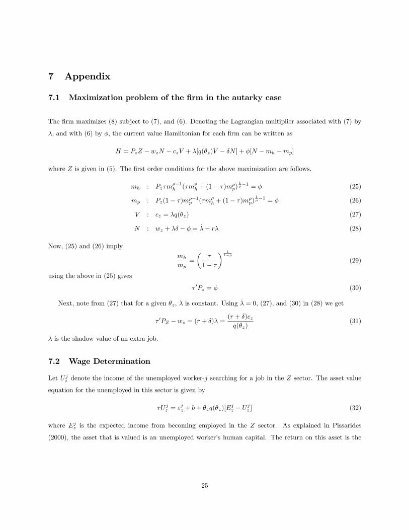
7.1 Maximization problem of the �rm in the autarky case

The �rm maximizes (8) subject to (7), and (6). Denoting the Lagrangian multiplier associated with (7) by

�, and with (6) by �; the current value Hamiltonian for each �rm can be written as

H = PzZ � wzN � czV + �[q(�z)V � �N ] + �[N �mh �mp]

where Z is given in (5). The �rst order conditions for the above maximization are follows.

mh : Pz�m��1h (�m�

h + (1� �)m�p)

1��1 = � (25)

mp : Pz(1� �)m��1p (�m�

h + (1� �)m�p)

1��1 = � (26)

V : cz = �q(�z) (27)

N : wz + �� � � =:

�� r� (28)

Now, (25) and (26) imply

mh

mp=

��

1� �

� 11��

(29)

using the above in (25) gives

� 0Pz = � (30)

Next, note from (27) that for a given �z, � is constant. Using:

� = 0; (27), and (30) in (28) we get

� 0PZ � wz = (r + �)� =(r + �)czq(�z)

(31)

� is the shadow value of an extra job.

7.2 Wage Determination

Let U jz denote the income of the unemployed worker-j searching for a job in the Z sector. The asset value

equation for the unemployed in this sector is given by

rU jz = "jz + b+ �zq(�z)[E

jz � U jz ] (32)

where Ejz is the expected income from becoming employed in the Z sector. As explained in Pissarides

(2000), the asset that is valued is an unemployed worker�s human capital. The return on this asset is the

25

unemployment bene�t b plus the expected capital gain from the possible change in state from unemployed

to employed given by �zq(�z)[Ez � Uz]:

The asset value equation for employed worker-j in sector Z is given by

rEjz = "jz + w

jz + �(U

jz � Ejz)) Ejz =

"jzr + �

+wjzr + �

+�U jzr + �

(33)

Again the return on being employed equals the wage plus the expected change in the asset value from a

change in state from employed to unemployed. Assume the rent from a vacant job to be zero which is ensured

by no barriers to the posting of vacancy. Now, denote the surplus for a �rm from a job occupied by worker-j

by Jjz . From (31) above this simply equals � 0PZ�wjz(r+�) : Since the wage is determined using Nash bargaining

where the bargaining weights are � and 1� �; we get the following wage bargaining equation:

Ejz � U jz = �(Jjz + Ejz � U jz ) (34)

The above implies that

Ejz � U jz =�

1� � Jjz =

�

1� �czq(�z)

(35)

where the last equality follows from the fact that the value of an occupied job, Jz; equals czq(�z)

as discussed in

(11) in the text. Plugging the value of Ejz �U jz from above into the asset value equation for the unemployed

in (32) we have a simpli�ed version of this asset value equation

rU jz = "jz + b+

�

1� � cz�z (36)

Next, (33) implies that

Ejz � U jz ="jzr + �

+wjzr + �

� rU jzr + �

(37)

Use (35) to substitute out Ejz�U jz and (36) to substitute out rU jz in the above expression to get the following

simpli�ed wage equation:

wjz = b+�cz1� � [�z +

r + �

q(�z)]

Note that wjz is the same for all j:Similarly, in the case of the X sector, we obtain wx = b+�cx1�� [�x +

r+�q(�x)

]:

7.3 Proof of Lemma 1

It is clear that for Pz < Pzo, the autarky domestic labor cost in sector Z is less than ws; and hence no

o¤shoring takes place. Therefore, even with the possibility of o¤shoring, the relative supply curve for p < po

is the same as the autarky relative supply curve.

26

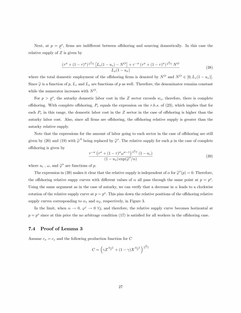
Next, at p = po; �rms are indi¤erent between o¤shoring and sourcing domestically. In this case the

relative supply of Z is given by

(�� + (1� �)�)1

��1�Lz(1� uz)�NO

�+ ��� (�� + (1� �)�)

���1 NO

Lx(1� ux)(38)

where the total domestic employment of the o¤shoring �rms is denoted by NO and NO 2 [0; Lz(1 � uz)]:

Since b' is a function of p; Lz and Lx are functions of p as well. Therefore, the denominator remains constantwhile the numerator increases with NO:

For p > po; the autarky domestic labor cost in the Z sector exceeds ws; therefore, there is complete

o¤shoring. With complete o¤shoring, Pz equals the expression on the r:h:s: of (23), which implies that for

each Pz in this range, the domestic labor cost in the Z sector in the case of o¤shoring is higher than the

autarky labor cost. Also, since all �rms are o¤shoring, the o¤shoring relative supply is greater than the

autarky relative supply.

Note that the expressions for the amount of labor going to each sector in the case of o¤shoring are still

given by (20) and (19) with b'A being replaced by b'o: The relative supply for each p in the case of completeo¤shoring is given by

������ + (1� �)�!��1

� ���1 (1� uz)

(1� ux) exp(b'o=�) (39)

where ui , !; and b'o are functions of p:The expression in (39) makes it clear that the relative supply is independent of � for b'o(p) = 0: Therefore,

the o¤shoring relative suppy curves with di¤erent values of � all pass through the same point at p = po:

Using the same argument as in the case of autarky, we can verify that a decrease in � leads to a clockwise

rotation of the relative supply curve at p = po: This pins down the relative positions of the o¤shoring relative

supply curves corresponding to �1 and �2; respectively, in Figure 3.

In the limit, when � ! 0; 'j ! 0 8j; and therefore, the relative supply curve becomes horizontal at

p = po since at this price the no arbitrage condition (17) is satis�ed for all workers in the o¤shoring case:

7.4 Proof of Lemma 3

Assume cx = cz and the following production function for C

C =� Z

��1� + (1� )X

��1�

� ���1

27

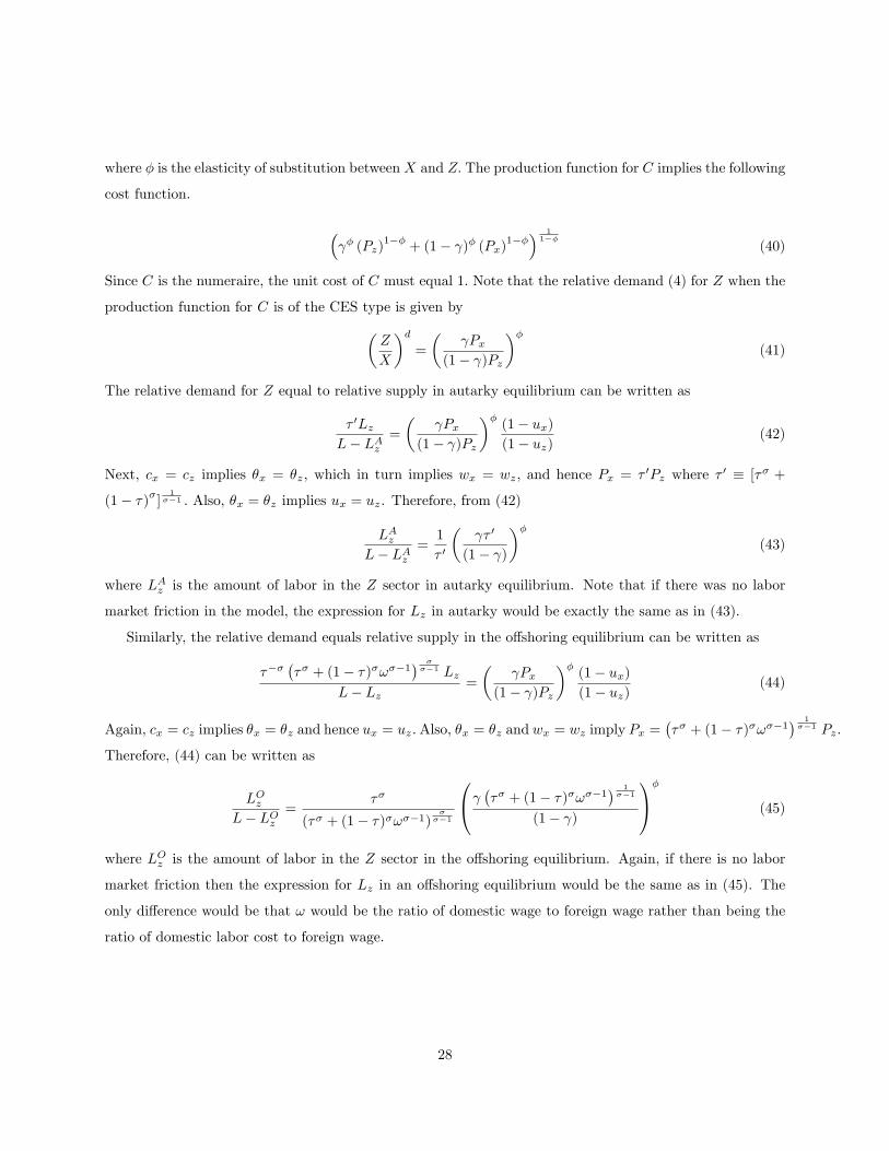
where � is the elasticity of substitution betweenX and Z: The production function for C implies the following

cost function.

� � (Pz)

1��+ (1� )� (Px)1��

� 11��

(40)

Since C is the numeraire, the unit cost of C must equal 1: Note that the relative demand (4) for Z when the

production function for C is of the CES type is given by�Z

X

�d=

� Px

(1� )Pz

��(41)

The relative demand for Z equal to relative supply in autarky equilibrium can be written as

� 0LzL� LAz

=

� Px

(1� )Pz

��(1� ux)(1� uz)

(42)

Next, cx = cz implies �x = �z, which in turn implies wx = wz; and hence Px = � 0Pz where � 0 � [�� +

(1� �)�] 1��1 : Also, �x = �z implies ux = uz. Therefore, from (42)

LAzL� LAz

=1

� 0

� � 0

(1� )

��(43)

where LAz is the amount of labor in the Z sector in autarky equilibrium. Note that if there was no labor

market friction in the model, the expression for Lz in autarky would be exactly the same as in (43).

Similarly, the relative demand equals relative supply in the o¤shoring equilibrium can be written as

������ + (1� �)�!��1

� ���1 Lz

L� Lz=

� Px

(1� )Pz

��(1� ux)(1� uz)

(44)

Again, cx = cz implies �x = �z and hence ux = uz:Also, �x = �z and wx = wz imply Px =��� + (1� �)�!��1

� 1��1 Pz.

Therefore, (44) can be written as

LOzL� LOz

=��

(�� + (1� �)�!��1)�

��1

0@ ��� + (1� �)�!��1� 1��1

(1� )

1A�

(45)

where LOz is the amount of labor in the Z sector in the o¤shoring equilibrium. Again, if there is no labor

market friction then the expression for Lz in an o¤shoring equilibrium would be the same as in (45). The

only di¤erence would be that ! would be the ratio of domestic wage to foreign wage rather than being the

ratio of domestic labor cost to foreign wage.

28

Comparing (43) and (45) note that LAz > (<)LOz if the following inequality holds.�

�� + (1� �)�

�� + (1� �)�!��1

���1��1

> (<)��

�� + (1� �)�!��1 (46)

We get the following possibilities:

Case I: � = 1: In this case the l.h.s of (46) exceeds the r.h.s if ��

��+(1��)�!��1 < 1; if which is true for

any �: Therefore, if the production function for C is Cobb-Douglas, then irrespective of the elasticity of

substitution in Z production, labor always moves from Z to X upon o¤shoring.

Case II: � = �: In this case the l.h.s of (46) exceeds the r.h.s if 1 +�1���

��> 1, which is always true

implying LAz > LOz :

Case III: � < 1; � > 1: In this case the l.h.s of exceeds 1 since ��+(1��)���+(1��)�!��1 < 1 and

��1��1 < 0; while the

r.h.s is less than 1. Therefore, again LAz > LOz :

Case IV: � < 1; � < 1: Again, the l.h.s of (46) exceeds 1 because ��+(1��)���+(1��)�!��1 > 1 and ��1

��1 > 0:

Therefore, again LAz > LOz :

Case V: � > 1; � > 1: Again, the l.h.s of (46) exceeds 1 because ��+(1��)���+(1��)�!��1 > 1 and ��1

��1 > 0:

Therefore, again LAz > LOz :

Case VI: � > 1; � < 1. In this case � < 1 implies ��+(1��)���+(1��)�!��1 > 1;but � > 1; � < 1 implies

��1��1 < 0:

Therefore, the l.h.s of (46) is less than 1. Since both the l.h.s and the r.h.s are less than 1, it is possible for

the r.h.s to exceed l.h.s in which case LAz < LOz :

7.5 Comparing equilibria with di¤ering degrees of labor mobility

We can also compare o¤shoring equilibria with di¤erent degrees of labor mobility using Figure 3. Since the

relative supply curves with di¤erent degrees of labor mobility all pass through the same point B at a price of

po in Figure 3, the impact of extent of labor mobility depends on whether the relative demand curve passes

to the left or right of point B in Figure 3, or whether the perfect mobility equilibrium is to the left of point

B or to the right of it. If in the perfect mobility case labor moves from sector Z to sector X; which is the

plausible scenario, as argued earlier, then we can show that the perfect mobility equilibrium at point C must

be to the left of point B as shown in Figure 3.

Proof: Note from (19) above that at b'A = 0; Lx = Lz = 12L; irrespective of �: That is, each sector has

exactly half of the labor in autarky equilibrium. Since (19) is also valid for o¤shoring with b'A replaced byb'o; the amount of labor in each sector must equal 12L because b'o = 0 at point B. Now, if labor moves from

29

Z to X in the case of o¤shoring equilibrium with perfect mobility, then the amount of labor in the X sector

in o¤shoring equilibrium must be greater than 12L: This in turn implies that the equilibrium Z=X must be

lower than at B:

7.6 ws and the likelihood of a mixed equilibrium under imperfect labor mobility

We �rst describe the shift in the relative supply curve in response to a decrease in ws: Recall from the

de�nition of po that it decreases as ws decreases: From the derivation of the o¤shoring relative supply curve,

a decrease in ws implies that the starting point of the o¤shoring relative supply curve slides down the autarky

supply curve. This implies that the horizontal segment of the o¤shoring relative supply curve slides down

the autarky relative supply curve as well. We can also verify that the rightmost point of the horizontal

segment is more to the left the lower the ws: To see this, note that the lower the ws the lower the �z and

consequently, the lower the Lz and the higher the uz: Therefore, verify from (38) that the relative supply

when NO = Lz(1 � uz) is lower the lower the ws: Finally, (23) implies that at any p the lower the wsthe higher the domestic labor cost in the Z sector. A higher domestic labor cost implies a higher �z and

hence a lower uz and a higher Lz. Therefore, at each p; the lower the ws the greater the relative supply.

Therefore, the o¤shoring relative supply curve shifts in response to a decrease in ws as shown in Figure 5 for

two di¤erent levels of ws(ws1 > ws2). From this �gure, it is clear that the likelihood of mixed equilibrium

goes down as ws goes down. The shift in the relative supply curve depicted in Figure 5 raises the possibility

of non-monotonicity of �z with respect to ws:

30

JC”JC’

JC

WCw

θ

Figure 1: Partial Equilibrium

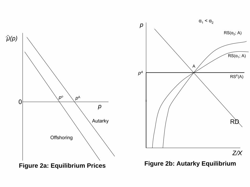
μ(p)

p

Figure 2a: Equilibrium Prices Figure 2b: Autarky EquilibriumZ/X

p

pARSP(A)

RD

RS(α1; A)

RS(α2; A)

A

α1 < α2

0pApo

Autarky

Offshoring

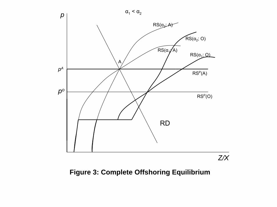
Figure 3: Complete Offshoring Equilibrium

p

pARSP(A)

RD

RS(α1; A)

RS(α2; A)

A

α1 < α2

RS(α1; O)

RSP(O)

RS(α2; O)

po

Z/X

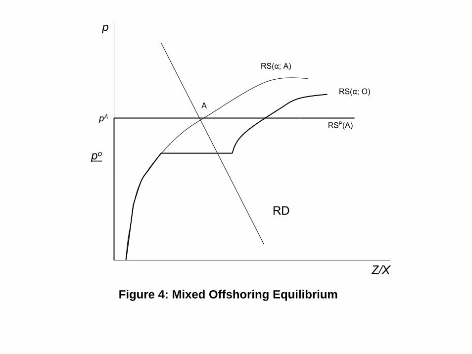
p

pA

RD

A

RSP(A)

Figure 4: Mixed Offshoring Equilibrium

po

Z/X

RS(α; A)

RS(α; O)

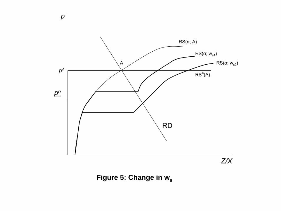
p

pARSP(A)

RD

A

po

Figure 5: Change in ws

RS(α; A)

RS(α; ws1)

RS(α; ws2)

Z/X