1

OIL PRICE AND EXCHAGE RATE VOLATILITY IN NIGERIA

BY

OYETUNJI BUSAYO

09AF09208

A B.Sc RESEARCH PROJECT SUBMITTED TO THE DEPARTMENT OF

ECONOMICS AND DEVELOPMENT STUDIES, COLLEGE OF DEVELOPMENT

STUDIES, COVENANT UNIVERSITY, OTA

2013

2

TABLE OF CONTENTS

CONTENT

Title page i

Certification ii

Dedication iii

Acknowledgement iv

Table of Contents v

List of Tables viii

List of Figures ix

Abstract x

CHAPTER ONE: INTRODUCTION

1.1 Background to the Study 1

1.2 Statement of Research Problem 3

1.3 Scope of study 4

1.4 Research Questions 5

1.5 Objectives of Study 5

1.6 Research Hypothesis 5

1.7 Definition of terms 5

1.8 Significance of Study 6

1.9 Research Methodology 7

1.10 Data Sources 7

1.11 Outline of Chapters 8

CHAPTER TWO: LITERATURE REVIEW

2.1 Review of Definitional Issues 9

2.1.1 History of Oil price 10

2.1.2 Brief History of oil in Nigeria 11

2.1.3 Exchange rate volatility 12

2.1.4 Various exchange rates Management Practised In Nigeria 13

2.1.5 Importance of Exchange rate stability 17

2.1.6 Measuring of Exchange rate Volatility 19

2.1.7 Oil Price and Exchange Rate 21

2.2 Review of Theoretical Issues 22

2.3 Review of Methodological and Empirical Issues 25

CHAPTER THREE: RESEARCH METHODOLOGY

3.1 Introduction 29

3

3.2 Theoretical Framework 29

3.3 Model Specification 32

3.3.1 Data sources and Descriptions 34

3.4 Research Methodology 35

CHAPTER FOUR: DATA PRESENTATION AND EMPIRICAL ANALYSIS

4.1 Introduction 41

4.2 Trend and Descriptive Analysis 42

4.3 Econometric Analysis 44

4.4 Findings and economic interpretation 48

4.5 Conclusion 49

CHAPTER FIVE: SUMMARY, CONCLUSION AND RECOMMENDATIONS

5.1 Summary 51

5.2 Policy Recommendations 51

5.3 Limitation of Study 53

5.4 Suggestions for further study 53

5.5 Conclusion 53

REFERENCES 54

APPENDIX 59

LIST OF TABLES

Table 1: Variables and Data sources

Table 2: Descriptive Statistics of Variables

Table 3: ADF Test and Phillips Perron Test for Unit Root

Table 4: Unrestricted Cointegration Rank Tests

Table 5: Normalized Co-integrating Co-efficient

Table 6: Vector Error Correction Estimates

4

LIST OF FIGURES

FIGURE 1: Diagram showing the Graphical relationship between EXRV, OILP, ER and INT

ABSTRACT

Nigeria is a mono-product economy, where the main export commodity is crude oil, changes in

oil prices has implications for the Nigerian economy and, in particular, exchange rate

movements. The latter is mostly important due to the double dilemma of being an oil exporting

and oil-importing country, a situation that emerged in the last decade. The study examined the

effects of oil price, external reserves and interest rate on exchange rate volatility in Nigeria

using yearly data from the year 1970 to 2011. The theoretical framework of this study is based

on Generalized Autoregressive Conditional Heteroskedasity modeled by Tim Bolerslev (1986)

and Exponential General Autoregressive Conditional heteroskedastic modeled by Daniel Nelson

(1991). The models are used to estimate the relationship between oil price changes and

exchange rate. Relevant descriptive and econometric analyses were employed. The econometric

tests used include the unit root tests, Johansen co-integration technique and the Vector Error

Correction Model (VECM) when the unit root tests were carried out; all the variables were

stationary at first difference. The long run relationship among the variables was determined

using the Johansen Co-integration technique while the vector correction mechanism was used to

examine the speed of adjustment of the variables from the short run dynamics to the long run. It

was observed that a proportionate change in oil price leads to a more than proportionate change

in exchange rate volatility in Nigeria by 2.8%. I therefore recommend that the Nigeria

government should diversify from the Oil sector to other sectors of the economy so that Crude oil

will no longer be the mainstay of the economy and frequent changes in crude oil price will not

influence exchange rate volatility significantly in Nigeria.

5

CHAPTER ONE

INTRODUCTION

1.1 BACKGROUND OF STUDY

“There are various evidences, particularly over the post-Breton woods era, pointing to the vital

role of oil price fluctuations in the determination of the path of the exchange rate” (Adeniyi et al,

2004). According to Krugman (1983), exchange rate appreciates in response to rising oil prices

and depreciates with response to falling oil prices in oil exporting countries, while the opposite is

expected to be the case in oil importing countries.

Volatility is the fluctuation in the value of a variable, especially price (Routledge, 2002).

According to Englama et al (2010), a volatile exchange rate makes international trade and

investments more difficult because it increases exchange rate risk. Exchange rate volatility tends

to increase the risk and the uncertainty of external transactions and predisposes a country to

exchange rate related risks (Jin, 2008).

According to Adedipe (2004), when Nigeria gained politically independence in October 1960,

agricultural production was the main stay of the economy, contributing about 70% of the Gross

domestic product (GDP), also employing about seventy percent of the working population and

responsible for about ninety percent of foreign government revenue. The initial period of post-

independence till mid – 1970s witness a fast advancement of industrialized capacity and output,

as the contributions made by the manufacturing sector to GDP rose from 4.8% to 8.2%. This

pattern changed when crude oil became very important to the world economy.

According to Englama et al (2010), crude oil became an export commodity in Nigeria in 1958,

following the discovery of the first producible well in 1956. The contribution of oil to the federal

government revenue in 1970 rose to 82.1% in 1974 from 26.3% and in 2008 constituted 83% of

6

the federal government revenue, largely on account of increase in oil prices in the international

market. The gigantic rise in oil revenue was caused by the Middle East war of 1973. It created

extraordinary, surprising and unforeseen wealth for Nigeria and the naira appreciated as foreign

exchange influxes offset outflows and Nigeria foreign reserves assets increased (Adedipe, 2004).

The economy of Nigeria gradually became dependent on crude oil as productivity declined in

other sectors (Englama et al, 2010).

Nigeria is a mono – product economy, according to OPEC statistical bulletin (2010/2011) the

value of Nigeria’s total export revenue in 2010 was US$70,579 million and the revenue of

petroleum exports from the total export revenue was US$61,804 million which is 87.6% of total

export revenue this means that Nigeria’s economy will be vulnerable to the movements of oil

prices.

During periods of favorable oil price shocks triggered by conflict in oil – producing areas of the

world, the rise in the demand for the commodity by the consuming nations, seasonality factors,

trading positions etc. Nigeria experiences favorable terms of trade evidenced by a large current

account surplus and exchange rate appreciation. On the converse, when crude oil prices are low,

occasioned by factors such as low demand, seasonality factors, excess supply, the Nigeria

experiences unfavorable terms of trade evidenced by budget deficit and slow economic growth

(Englama, 2010). An example was a drop in the revenue from oil exports during the global

financial crisis in 2009. According to, OPEC statistical bulletin (2010/2011), oil export revenue

dropped from US$74,033 million in 2008 to US$43,623 million in 2009 and the naira

depreciated to N148.902 in 2009 from N118.546 in 2008.

7

This study attempts to discover the extent to which oil price influences exchange rate volatility in

Nigeria. Oil price changes directly affects the inflow of foreign exchange into the country,

therefore there is a need to investigate its impact on the naira exchange rate volatility (Englama

et al, 2010).

1.2 STATEMENT OF PROBLEM

Crude Oil is a key source of energy in Nigeria and the in the world. Oil being an important part

of the economy of Nigeria plays a strong role in influencing the economic and political fate of

the country. Crude oil has generated great wealth for Nigeria, but its effect on the growth of the

Nigerian economy as regards returns and productivity is still questionable (Odularu 2007).

From the period of the oil boom of the 1970s till now, Nigeria has neglected her strong

agriculture and light manufacturing bases in favor of unhealthy dependence on crude oil. New oil

wealth has led to a concurrent decline of other sectors in the economy and has fueled massive

migration to cities and led to increasingly wide spread poverty especially in rural areas. Nigeria’s

job market has witnessed very high degree of unemployment, small wage and pitiable working

environments (Adedipe, 2004 and Odularu 2007). Between 1970 to 2000, Nigeria’s poverty rate

increased from 36 percent to just fewer than 70 percent and it is believed that oil revenue did not

seem to add to the standard of living at this time but actually caused it to decline (Martin and

Subramanian, 2003).

Oil price fluctuations have received important considerations for their presumed role on

macroeconomic variables. Higher oil prices may reduce economic growth, generate stock

exchange panics and produce inflation which eventually leads to monetary and financial

instability. It will also lead to high interest rates and even a plunge into recession (Mckillop,

8

2004). Sharp increases in the international oil prices and the violet fluctuations of the exchange

rate are generally regarded as the factors of discouraging economic growth (Jin, 2008).

A very good example is the period of the global financial crisis, the price of oil fell by about two

thirds from its crest of $147.0 per barrel in July 2008 to $41.4 at end of December 2008. Before

the crises, oil price was high, exchange rate was stable but with the dawn of the global financial

crisis (GFC) oil price crashed and the exchange rate caved-in, depreciating by more than 20 per

cent. Since oil price volatility directly affects the inflow of foreign exchange into the country,

there is a need to investigate if it has direct impact on the Naira exchange rate volatility

(Englama et al, 2010)

The oil market has been and will continue to be an ever changing arena. This is because oil is so

vital to the world economy, it is present in everyone’s daily lives and its market is truly global

(El – badri, 2011).

Thus, it is on this note that this research seeks to find out the effect of oil price on exchange rate

volatility and its effects on the Nigerian economy, as well as suggest methods of minimizing the

adverse effects it can produce on the economy as a whole.

1.3 SCOPE OF STUDY

The purpose of the study is to determine the relationship between oil price and exchange rate in

the Nigerian economy. 1t covers the period between 1970 and 2011.

9

1.4 RESEARCH OUESTIONS

The study attempts to give answers to the following questions

1. Do oil price have a significant relationship with exchange rate volatility in Nigeria?

2. What is the long run impact of oil price on exchange rate volatility in Nigeria?

1.5 OBJECTIVES OF THE STUDY

The major objective for this research is to determine if a long run relationship exists between oil

price and exchange rate in Nigeria. The specific objectives include:

1. To examine if there exists a significant relationship between oil price and exchange rate

volatility in Nigeria.

2. To assess the long run impact of oil price on exchange rate volatility in Nigeria.

1.6 RESEARCH HYPOTHESIS

In effort to realize the objectives of the study, the following hypothesis will be tested:

H0: Oil price has no statistical significant effect on exchange rate volatility in Nigeria

H1: Oil price has a statistical significant effect on exchange rate volatility in Nigeria

H0: There is no long run relationship between oil price and exchange rate volatility in

Nigeria

H1: There is a long run relationship between oil price and exchange rate volatility in

Nigeria

10

1.7 DEFINITION OF TERMS AND CONCEPTS

VOLATILITY: Fluctuations in the value of a variable, especially price.

OIL - PRICE: The price in dollars at which a barrel of crude oil is sold for in the international

market.

EXCHANGE RATE: The price of one currency in terms of another. It can be expressed in one of

two ways, as units of domestic currency per unit of foreign currency or units of foreign currency

per unit of domestic currency

ECONOMIC GROWTH: This is the growth of the real output of an economy overtime.

EXCHANGE RATE VOLATILITY: It refers to the swings of fluctuations in the exchange rates

over a period of time or the deviations from a benchmark or equilibrium exchange rate.

OPEC: Organization of Petroleum Exporting Countries. It consists of twelve members which

includes Nigeria.

1.8 SIGNIFICANCE OF STUDY

Researches conducted in this field of study have found out that oil price influence exchange rate

to a great extent, especially oil producing countries. Nikbakbt (2009) showed that real oil prices

have been a dominant source of real exchange rate movement and there exist a long run and

positive linkage between real oil price and real exchange rates for OPEC countries. Oil

exportation has contributed positively to Nigeria GDP, local expenditure, government revenue

and foreign exchange reserves (Odularu 2007). Also in the words of Adedipe (2004) the oil price

influences government policy and exchange rate in Nigeria.

11

Although a wealth of literature exist relating oil price and exchange rate to economic growth in

Nigeria, little focus on the effect of the oil price on exchange rate in Nigeria. This project seeks

to fill this gap in literature as it focuses on the effect of oil price on exchange rate volatility in

Nigeria and whether or not it has a significant influence on exchange rate volatility in Nigeria.

Thus, this study is of great benefit to the government and policy makers. It reemphasizes the

need to diversify and promote the growth of other sectors of the economy, in other to increase

economic growth and improve the standard of living for Nigerians.

1.9 RESEARCH METHODOLOGY

Econometric technique will be used to analyze the effect of Oil price on exchange rate in

Nigeria. The GARCH (1, 1) model is used to measure exchange rate volatility and the

conditional variance series generates the volatility data from 1970 – 2011. The method adopted

in determining a long run relationship between oil price and exchange rate volatility is the

Johansen co-integration technique and the Vector Error Correction Model (VECM) specifies the

convergence or divergence among the variables in the model.

1.10 DATA SOURCES

The study will make use of secondary data and it will be sourced from the central bank of

Nigeria statistical bulletin 2011, BP statistical review on energy 2012 and exchange rate

volatility is represented by conditional variances which will be generated using E-Views 5.0

12

1,11 OUTLINE OF CHAPTERS

This study is divided into five chapters. Chapter one which is the present chapter, gives a general

overview of the study. Chapter two reviews papers related to this topic. It includes theoretical

issues, empirical issues and the results of research relating to this topic.

The third chapter focuses on the research methodology it includes, technique of estimation,

model specification and it also employs statistical technique in finding statistical relationship

between the variables. Chapter four involves the presentation of data, analysis and discussion of

results in chapter three. Lastly, chapter five, summarizes the major findings in this research

study, concludes and gives policy implications of findings.

13

CHAPTER TWO

LITERATURE REVIEW

2.1 REVIEW OF DEFINATIONAL ISSUES

The crude oil price and exchange rates are key research subjects, and both variables generate

considerable impacts on macroeconomic conditions such as economic growth, international

trade, inflation, and energy management. The relationships between the two have been studied,

mainly for guidelines of interaction and causality. In past decades, changes in the price of crude

oil have been shown to be a key factor in explaining movements of foreign exchange rates,

particularly those measured against the U.S. dollar (Huang and Tseng, 2010).

While a considerable amounts of studies have dealt with some aspect of the relationship between

international oil price and exchange rate, a number of questions still spring to mind namely: Is

there a role of oil prices in exchange rate determination in Nigeria, Do positive and negative

shocks to oil prices volatility have symmetric effect on exchange rate volatility? Among other

questions (Adeniyi, Omisakin, Yaqub and Oyinlola, 2012).

This section brings together relevant literature regarding oil price and exchange rate. Brief

reviews are given with respect to the history of oil prices, history of crude oil in Nigeria,

Exchange rate volatility, various exchange rate management system practiced Nigeria,

importance of exchange rate stability, measuring of exchange rate volatility and the relationship

between oil price and exchange rate in Nigeria. Theoretical and methodological issues on the

topic are also looked at.

14

2.1.1 HISTORY OF OIL PRICES

Since the ending of the 1940s to the begining 1970s the international oil price was very steady

having only small changes. Then from the early 1970 to the early 1980s the price of oil increased

beyond expectation with respect to the rise of OPEC and the disruption in the supply of crude oil.

OPEC first experienced the power it had over oil during Yom Kippor War which started in 1973.

OPEC imposed an oil restriction on western countries as a result of US and the Europe support

for Israel. Production of Oil was reduced by five million barrels a day. The cut back amounted to

about seven percent of the world production and the price of oil increased 400 percent in six

months.

From 1974 to 1978 crude oil prices were relatively stable ranging from $12 to $14 per barrel.

Then between 1979 and 1980 during the Iranian revolution and Iraq war world oil production fell

by 10% and caused the rise of crude oil from $14 to $35 per barrel. Oil prices were leading

consumers and firms to adopt a more conserve energy. People purchased cars that could manage

fuel and organizations purchased machine that were more fuel efficient (Sharma 1998).

Increased oil price also enlarged search and production by nations that were not members of

OPEC. Beginning from 1982 to 1985 OPEC wanted to steady the price of oil through production

of quotas, but safeguarding efforts, global economic meltdown and wrongful quotas produced by

OPEC participant countries contributed to the plunging of oil prices beneath $10 per barrel.

From the Mid – 1980s the fluctuations in the price of oil has occurred more frequent than the

past. OPEC has continually been trying to influence oil price to ensure its stability through

allocation of production quotas to its member countries but has been unable to stabilize it. OPEC

share of the world oil production has fallen from 55 percent in 1976 to 42% today.

15

Oil prices matter in the economy in various ways. Changes in oil price directly affect

transportation costs, heating bills and the prices of goods made with petroleum products. Oil

price spikes induce greater uncertainty about the future, which affects households and firms

spending and investments decisions. Also changes in oil prices leads to reallocations of labor and

capital between energy intensive sectors of the economy and those that are non-energy intensive

sector. (Sill, 2009).

2.1.2 BRIEF HISTORY OF OIL IN NIGERIA

The search for oil began in 1908 by a German company named Nigeria Bitumen Corporation,

but there was no success until 1955 when oil was discovered in Oloibiri in Niger delta by shell-

BP. Nigeria started exporting crude oil in 1958 but in major quantity started to flow in 1965,

after the establishment of the bonny island on the coast of Atlantic and the pipeline to link the

terminal.

In 1970, as the Biafra war was ending there was a rise in world oil price and Nigeria benefited

immensely from this rise. Nigeria became a member of Organization of petroleum exporting

countries (OPEC) in 1971 and the Nigerian National Petroleum company (NNPC) which is a

government owned and controlled company was founded in 1977. By the late sixties and early

seventies, Nigeria had attained a production level of over 2 million barrels of crude oil a day.

Although there was a drop in production of crude oil in the eighties due to economic down turn,

by 2004 Nigeria bounced back producing 2.5 million barrels per day, but the Niger delta crisis

and the global economy financial crises reduced Nigeria oil production and the world oil price.

The discovery of oil brought in the eastern and mid – eastern regions of Nigeria brought hope of

a brighter future for Nigeria in terms of economic development as Nigeria became independent,

16

but there were also grave consequences of the oil industry, it fuelled already existing ethnic and

political tension. The tension reached its peak with the civil war and reflected the impact and fate

of the oil industry.

Nigeria survived the war and was able to recover mainly from the huge revenue gained from oil

in the 1970s. Nigeria gained a lot from the three year oil boom. There was a lot of money to meet

all our development need. The oil revenue which was supposed to be a blessing became a cause

because of the corruption and the mismanagement of revenue from oil. The enormous impact of

the oil shock on Nigeria grabbed the attention of scholars and they tried to analyze the effect of

oil price on economic growth in Nigeria. A set of radical oriented writers were interested in the

nationalization that took place during the oil shock as well as the linkages between oil and an

activist foreign policy. Regarding the latter, the emphasis was on OPEC, Nigeria's strategic

alliance formation within Africa, the vigorous efforts to establish the Economic Community of

West African States (ECOWAS), and the country's attempts to use oil as a political weapon,

especially in the liberation of South Africa from apartheid.

Many people had hoped that Nigeria will become an industrial nation and a prosperous nation

from the benefits of oil but they were greatly disappointed when we Nigeria hit a major financial

crisis that led to the restructuring of the economy (Odularu, 2007; Ogundipe and Ogundipe 2013)

2.1.3 EXCHANGE RATE VOLATILITY

It is well-known in literature that getting the exchange rate right or maintaining relative stability

is important for both internal and external balance and consequently growth in the economy.

Exchange rate is the most important price variable in an economy and performs the twin role of

17

maintaining international competitiveness and serving as nominal anchor to domestic price

(Mordi 2006).

Swings or fluctuations in the exchange rates over a period of time or deviations from a

equilibrium exchange rate is referred to exchange rate volatility. Where there is multiplicity of

markets parallel with the official market there could be deviations from the equilibrium exchange

rate. Volatility over any time period interval tends to increase when supply, demand or both are

likely to respond to large random shocks and when the elasticity of both supply and demand is

low price volatility tends to be low (Obadan 2006)

The exchange rate is subjected to variations when it is not fixed, thus floating exchange rate

tends to be more volatile. Economic essentials affect the level of volatility and the extent to

which exchange rate stability is maintained. Favorable economic circumstances and outcome

which in turn would appreciate the currency and maintain stability is caused by strong

fundamentals. (Mordi 2006)

2.1.4 VARIOUS EXCHANGE RATE MANAGEMENT PRACTISED IN

NIGERIA

Nigeria exchange rate moved from a fixed regime in the 1960s to a pegged arrangement between

the 1970s and the mid-1980s, and to end with various types of the floating regime since 1986,

following the adoption of the Structural Adjustment Programme (SAP). A regime of managed

float has been the most important feature of the floating regime in Nigeria since 1986without any

strong compulsion to protecting any particular parity.

Fixed exchange rate regime practiced in Nigeria led to an over appreciation of the Nigerian

currency and it was encouraged by the exchange regulator guidelines that produced noteworthy

18

alterations in the Nigerian economy. This led to a rise in importation of finished goods beyond

expectation and it had terrible effect on internal production, Nigeria’s balance of payment

situation and Nigeria’s foreign reserve level. This situation and many other issues encouraged the

adoption of a more flexible exchange rate regime which is the SAP regime in 1986.

A continued distortion of the value of exchange rate in the market for foreign exchange rate will

cause a hostile effect on Nigeria’s economic performance in the medium term. Therefore, the

Nigerian authorities should react to changes in the equilibrium exchange rate on time. Given the

structure of the Nigerian economy, maintenance of a realistic exchange rate for the naira is very

vital, and the need to reduce fluctuations in production and consumption, increase the inflow of

non-oil export receipts and attract foreign investments.

Fixed exchange rate regime requires the fixing of the local currency exchange rate to a piece of

gold, a locus currency like the dollar or a bag of monies or the SDR, with the main goal of

maintaining a small rate of inflation. The rewards and shortcomings of the fixed regime have

been acknowledged very well in a number of literature. It includes but is not limited a reduction

in the cost of trading, increase in macroeconomic stability, dependability increase due to stability

in the exchange rate and improved response to local nominal shocks. A main drawback of the

fixed exchange rate regime, however, is that it infers the damage of monetary policy

independence.

The activities of demand and supply will control the exchange rate in a floating exchange

regime. This system believes that there is no hand controlling the foreign exchange market even

the government and that the exchange rate corrects to any shortfall or excess in the foreign

exchange market without the intervention of the public. This means that any change in the

demand and supply of foreign exchange can change the exchange rates but cannot change the

19

reserve position of the country. In this arrangement, the exchange rate assists as a “jumbo” for

outside shocks, therefore permitting the monetary authorities complete discretion in the

demeanor of monetary policy. The drawbacks of the freely floating exchange rate system have

been known. It include insistent exchange rate variations, increased inflation and increased

transaction cost. The best advantage of the floating exchange rate system, is monetary policy

freedom, explained by a country’s capacity to influence its monetary totals and control its

national interest rate and inflation.

An adjustment to the freely floating system is managed floating system which exists when the

local government interferes in the market for foreign exchange in order to regulate movements in

the exchange rate. It does not obligate itself to maintain a fixed exchange rate or some thin limits

round it.

From the Inception of the CBN, Nigeria’s exchange rate policy goal has aimed at conserving the

outside value of the local currency and upholding a solid position of the balance of payments,

which, certainly, is a foremost provision of the aiding law. The disappointment of the

Autonomous Foreign Exchange Market (AFEM), which was presented in 1995, led to an Inter-

Bank Foreign Exchange Market (IFEM) was presented on October 25, 1999. The initial plan of

the IFEM was to be mutual quote system. It intended to vary the foreign exchange supply in the

economy by boosting the financing of the inter-bank jobs from foreign exchange earned

privately. IFEM goal was also aimed at encouraging the naira to attain an applied exchange rate.

IFEM operations also experienced comparable glitches and delays as the AFEM. This was

caused by inflexibilities on the supply side, the repeated expansionary fiscal activities by the

Nigerian government and the resultant difficulty of consistent surplus liquidness in the system.

Central Bank of Nigeria introduced the Dutch Auction System (DAS) again to remove the IFEM.

20

This system was created to accomplish a stable exchange rate of the naira that will lessen the

undue demand for foreign exchange, safeguard the reducing level of external reserves and

accomplish a genuine exchange rate for the Nigerian currency. The DAS was perceived as a

give-and-take auction system in which CBN and legal dealers together will partake in the market

of foreign exchange rate to buy and sell foreign exchange. CBN is required to decide on the

quantity of foreign exchange it wants to sell and at the price that buyers will be willing to buy.

The marginal rate is the “presiding” rate at the auction, which means it is the rate that clears the

market.

The foreign exchange earnings of Nigeria are over ninety percent dependent on the revenue from

crude oil exports. The consequence of this action means that unpredictability of the world’s oil

prices has an immediate impact on the supply of foreign exchange in Nigeria. Also, Nigeria’s oil

sector generates over eighty percent of the government revenue in Nigeria. Therefore, an

increase in the world oil prices leads to a higher revenue shared between the federal, state and

local government of Nigeria and this has been the trend since the early1970s, expenses also

increases in the same manner and it is difficult to bring down when oil prices falls down and

revenues falls together with it. There is no doubt that such unpredictable expenditure level has

been the main cause of Nigeria government deficit spending. It is for this very reason that

foreign reserves are maintained by the government so that the expenditure needs of the country

can be met when the price of oil decreases in the international oil market. A key concern is the

economic situation in Nigeria, position in the outside economic setting and the consequence of

several hit and misses jolts on the local economy. Hence, nations like Nigeria are most likely to

take up a system which guarantees more flexibility because they are easily affected by unstable

inner financial circumstances and outside shocks, which needs real exchange rate to depreciate,.

21

On the whole, there is a overall agreement that a fixed exchange rate system should be taken up

if what causes macroeconomic volatility is mostly internal. While a flexible exchange rate

system is favored if volatility are mainly external in nature. Therefore it is becoming increasingly

accepted that irrespective of what exchange rate system a country adopts, the overall

achievement rests on its obligation to maintain sound economic nitty-gritties and a good banking

system (Sanusi 2004).

Schnabl (2007) argued that theoretically flexible exchange rate makes it easier for a country to

adjust to asymmetric specific real shocks. Whereas, the micro economic effects of low exchange

rates fluctuations under fixed exchange rate system are linked to reduced transaction costs for

international trade and capital flows thereby increasing economic growth. If exchange rate

volatility is eliminated, international arbitrage enhances efficiency, productivity and welfare.

2.1.5 IMPORTANCE OF EXCHANGE RATE STABILITY

1. When exchange rate is stable it increases the standard of living of the people by helping

to decrease the uncertainty about general price developments and in so doing improve the

transparency of general prices.

2. It leads to reduction in inflation risk premia in interest rates: if creditors are certain that

prices will remain stable in the future, they will not demand for an extra return (risk

premium) to compensate them for the inflation risks associated with holding nominal

assets over the longer term. It increases the incentive to invest because the capital market

allocates resources more efficiently. This again fosters job creation and, more generally,

economic welfare.

22

3. It also helps to circumvent unnecessary hedging risk: The maintenance of exchange rate

stability will make it less likely for individuals and firms to redirect resources from

productive uses in order to hedge themselves against inflation or deflation, for example

by indexing nominal contracts to price developments. Since full indexation is not feasible

or is too costly, in a high-inflation environment there is an reason to stockpile real goods

given that in such circumstances they retain their value better than money or certain

financial assets. An excessive stockpiling of goods hinders economic and real income

growth because it is not an efficient investment decision.

4. It increases the benefits of holding cash: Inflation can be interpreted as a unknown tax on

holding cash. This means that, people who hold cash (or deposits which are not rewarded

at market rates) experience a decline in their real money balances and thus in their real

financial wealth when the price level rises, just as if part of their money had been taxed

away. Therefore, the higher the anticipated rate of inflation, leads to a fall in demand by

households for cash holdings. This happens when inflation is fully expected, that is

inflation is uncertain. Consequently, if people do not hold a lot of cash, they must make

more regular visits to the bank to withdraw money. In general, reduced cash holdings can

be said to generate higher transaction costs.

5. It contributes to financial stability: Unexpected revaluations of assets owing to

unforeseen changes in inflation can undermine the reliability of a bank’s balance sheet.

For example, let us assume that a bank provides long-term fixed interest loans which are

financed by short-term time deposits. If there is a sudden shift to high inflation, this will

mean a fall in the real value of assets. Following this, the bank may face solvency

problems. If monetary policy maintains price stability, inflationary order inflationary

23

shocks to the real value of nominal assets are avoided and financial stability is therefore

also enhanced.

6. Maintenance of a constant exchange rate contributes to broader economic goals: In

summary all of these arguments suggest that a central bank that maintains exchange rate

stability contributes substantially to the achievement of broader economic goals, such as

higher standards of living, high and more stable levels of economic activity and

employment (European central bank, 2007)

2.1.6 MEASURING OF EXCHANGE RATE VOLATILITY

In the vast wide-ranging literatures on exchange rate volatility, there has been no agreement on

the appropriate approach for evaluating volatility by economic researchers. The lack of an

agreement on this topic echoes a number of factors as different theories cannot provide a definite

guidance as to which measure is the most suitable. Moreover, the type of measure to be adopted

will depend on the scope of study. The time period over which fluctuations is to be measured, as

well as whether it is unrestricted volatility or the sudden movement in the exchange rate parallel

to its predicted value needs to be taken into consideration. Finally, in shaping the applicable

measure of exchange rate to be used, the level of collective trade flows should be taken into

consideration.

The degree to which exchange rates, due to its habitually high volatile state are a source of risk

and ambiguity depends on the degree to which movements in the exchange rate are predictable.

With hedging, the predictable part can be hedged away so that the cost on trade is minimal. A

realistic measure would be to use the forward rate as an sign of the future spot rate, and

indicating the exchange rate risk with the discrepancies between the current spot rate and the

24

earlier period forward rate even though using the forward rate as an indicator as a problem with

predicting the future exchange rates adding to the fact that quotations are only existing for major

currencies.

McKenzie (1999) believes that there are a number of measures that should be taken into

consideration ranging from the structural models to the time series equation making use of the

ARCH/GARCH approaches. The standard deviation of the first variation of logarithms of the

exchange rate is the most widely used in measuring exchange rate volatility. If the exchange rate

is on a steady trend, which could easily be forecasted the result will therefore not be a source of

uncertainty. The standard deviation is calculated over a period of one year to point out a short-

run volatility and in acquiring long-term variability, a period of five years is used.

Finally, in measuring exchange rate volatility, the importance of currency invoicing is to be

taken into consideration. Mostly, trade between two developing countries is not invoiced in the

currency of either country. A standard currency is been used mostly the U.S. dollars is often used

as the invoicing currency. It may look like the volatility of the exchange rate between the two

trading partners’ currencies is not the important volatility to consider however this is wrong. For

example, if trade exports from China to Nigeria are invoiced in U.S. dollars, it might look like

the Chinese exporters would only care about the changes between the U.S. dollar and the

Chinese Yuan, but not between the Nigeria naira and the Chinese Yuan. Nevertheless, any

change between the Chinese Yuan and the Nigeria naira holding constant the Chinese Yuan/U.S.

dollar rate must mirror fluctuations in the Nigeria naira/U.S. dollar rate. As the latter could affect

the Nigerian demand for Chinese exports, changes in the Chinese Yuan/Nigeria naira exchange

rate would also affect the Chinese exports to Nigeria even if the trade is invoiced in the U.S.

dollar (Ojebiyi and Wilson 2011)

25

2.1.7 OIL PRICE AND EXCHANGE RATE

According to Adedipe (2004) the different exchange rate regimes in Nigeria can be classified

into different periods relating to vagaries in the international oil market.

1. The Post-Independence Era (1960 – 1971)

The Nigerian currency was pegged at par to the British pound sterling (GBP) using

administrative measures, to sustain the parity. The devaluation of GBP in 1967 made Nigeria

adopt the US dollar, which was deemed better to support the import substitution industries which

depend heavily on net imported inputs. Throughout this period the Nigerian pound sterling was

overvalued, inhibiting optimal growth in agriculture and in goods produced for exports.

2. The Oil Boom Era (1972 – 1986)

During this period the exchange rate moved in the same pattern as the oil prices and the naira

remained overvalued as a result of the huge increase in foreign exchange earnings. This currency

was anchored to the GBP until, 1972 when the GBP was floated and then pegged to the US

dollar. However in 1978, the naira was anchored on a basket of currencies of Nigeria 12 major

trading partners. This was changed in 1985 and the Naira reverted to quotation against the US

dollars.

3. The Post – Sap Era (From 1986)

The Naira was subject to a managed float system in a continuing effort to restructure the

economy away from oil dependency. The policy of deregulation of the foreign exchange market

in 1986 was to show the true value of the naira, this was in the view of boosting oil-non exports.

26

Thus, from N0.89388/US$ at the end of 1985, the exchange rate weakened to N2.0206/$ at the

end of 1986. This was done in expectation of promotion of non-oil exports and the naira was

further devalued in March 1992 by 44% to N17.2984/$. Devaluation of the naira in other to

encourage non-oil export has not produced the desired return.

The Exchange rate value of Nigeria is very crucial to the Annual budget, the Gross domestic

product (GDP), the level of development, among other things. Therefore, a study on the effect of

Oil price on Exchange rate volatility is very important.

2.2 REVIEW OF THEORECTICAL ISSUES

Diverse theoretical relationship between oil price and exchange rates have been established in

literature (Beckmann and Czudaj 2012). Oil price fluctuations have received significant

considerations for their believed role in macroeconomic variables. The consequences of large

increases in the oil price on macroeconomic variables have been of great concern among

economist and policy makers as well as the general public, since two major oil price shocks hit

the global economy in the 1970s (Sill 2009)

The thought that exchange rate is the most difficult macroeconomic variable to model

empirically is debatable. Many papers have suggested that oil price might have a significant

influence on exchange rate. The proposition that oil price might be adequate enough to explain

all the long run movements in real exchange rate appears to be new (Al-Ezzee, 2011)

Nigeria like among other low income countries has adopted two main exchange rate regimes for

the purpose of gaining balance both internally and externally. The purpose for this different

27

practice is to maintain a stable exchange rate (Umar and Soliu 2009). A fluctuating real exchange

rate as a result of adverse fluctuation stemming from volatile oil prices are damaging to non – oil

sector, capital formation and per capita income (Serven and Solimano 1993 and Bagella 2006).

The consequences of substantial misalignments of exchange rate can lead to shortage in output

and extensive economic hardship. There is reasonably strong evidence that the alignment of

exchange rate has a substantial influence on the rate of growth of per capita output in low income

countries (Isard 2007).

According to Trung and Vinh (2011) there are two reasons why macroeconomic variables should

be affected by oil shocks. First, oil increase leads to lower aggregate demand given that income

is redistributed between net oil import and export countries. Oil price spikes could alter

economic activity because household income is spent more on energy consumption and firms

reduce the amount of crude oil it purchases which then leads to underutilization of the factors of

production like labor and capital. Second, the supply side effects are related to the fact that crude

oil is considered as the basic input to production process. A rise in oil price will lead to a decline

in supply of oil because of the rise in cost of crude oil production which will lead to a decline in

potential output.

For various reasons known and unknown, oil price increases may lead to significant slowdown in

economic growth. Five of the last seven United States of America recessions were preceded by

significant increases in the price of oil (Sill, 2009). A factor discouraging economic growth is

sharp increases in the international price of oil (Jin, 2008).

28

Analysis of the impact of asymmetric shocks caused by exchange rate and oil price variability on

economic growth has been a major concern of both academics and policy makers for a long time

now (Aliyu 2009). According to Amano and Norden (1998) many researchers suggest that oil

fluctuations has a significant consequence on economic activity and the effect differ for both oil

exporting countries and oil importing countries. It benefits the oil exporting countries when the

international oil price is high but it poses a problem for oil importing countries.

According to Plante (2008) theoretically immediate effect of positive oil price shocks is the

increase in the cost of cost of product for oil importing countries , this is likely to reduce output

and the magnitude of the depends on the demand curve for oil. Higher oil prices lower

disposable income which then leads to a decrease in consumption. Once the increase in oil price

is believed to be permanent, private investments will decrease. But if the shocks are perceived as

persistent oil is used less in production, the productivity of labor and capital will decline and

potential output will fall.

Some researchers have carried out research the issue of oil price and exchange rate further.

According Rickne (2009) political and legal institutions affect the extent to which the real

exchange rate of oil exporting countries is affected by international oil price shocks. In a

theoretical model strong institutions protect real exchange rate from oil price volatility by

generating a smooth pattern of fiscal spending over the price cycle. Empirical analysis carried

out on 33 oil exporting countries show that countries with high bureaucratic quality and strong

and impartial legal system have real exchange rate that are affected less by oil price. Also

29

according to Mordi and Adebiyi (2010) the asymmetric effect of oil price changes on economic

activity is different for both oil price increase and oil price decrease. Patti and Ratti (2007) shows

that oil price increases have a greater influence on the economy than a decrease in oil price.

2.3 REVIEW OF METHODOLOGICAL AND EMPIRICAL ISSUES

Empirical research on the part of oil price plays as a determinant of real exchange rate has

yielded somewhat puzzling results for oil exporting countries. (Rickne, 2009)

According to empirical works carried out, there has been what appears to be a rather strong

relationship between real oil prices and real exchange rates of a number of countries (Plante

2008).

Korhonen and juurikkala (2007) showed that increasing crude oil prices cause a real exchange

rate appreciation in oil exporting countries and this is not shocking, since they earn a significant

amount from oil exportation. There is also a significant relationship between real oil prices and

real exchange rates for oil importing countries; evidence has been seen for Spain (Camarero and

Tamant 2002).

A study carried out on the Russian economy by Spatafora and Stavrev (2003) confirm the

sensitivity of Russia’s equilibrium real exchange rate to long run oil prices. Likewise, Suseeva

(2010) verified a long run positive relationship between the real oil price and the real bilateral

exchange rate against Euro in Russia. Lizardo and Mollick (2010) provided proof that between

the year 1970s to 2008, movements in the value of the U.S dollar against major currencies was

significantly explained by oil prices. They found that when oil prices group currencies of oil

30

importers such as china suffer depreciation. On the other hand, in net oil exporters such as

Canada, Mexico and Russia increase in oil prices leads to a noteworthy depreciation of the US

dollar. But, Akram (2004) finds strong evidence of no linear relationship between oil prices and

the Norwegian exchange rates.

Using Blanchard – Quah identification strategy Clarida and Gali (1999) estimate the share of

exchange rate fluctuations that is due to the different shocks in oil. Using quarterly data from

1974 to 1992 comparing the United States of America to four different countries (Germany,

United Kingdom, Japan and Canada) they found that more than 50% of the variance of real

exchange rate changes over all the horizons was caused by real oil shocks. Amano and Norden

(1998) using data on real effective exchange rates for Germany, Japan and United States of

America discovered that real oil price is the most important factor in determining real exchange

rates in the long run.

An advance in the productivity of tradable relative to non-tradable if larger in other countries

could lead to the appreciation of the real exchange rate. This is the Balassa-Samuelson

hypothesis formulated by Balassa (1964) and Samuelson (1964). According to Coudert (2004),

the Balassa-Samuelson effect is the mechanism by which an appreciation of the real exchange

rate occurs owing to changes in relative productivity. We use the real oil price as a representation

of the terms of trade and examine the influence of oil price fluctuations and productivity

differentials on the real exchange rate given that oil price is the main export good driving the

terms of trade in oil exporting countries. In practice, the price of the main exported good is often

used as an indicator of the terms of trade (Sossounov and Ushakov, 2009).

31

Using a panel of 16 developing countries Choudhri and Khan (2004) provided strong evidence of

the workings of the Balassa Samuelson effects. Coudert (2004) survey provided evidence that the

trend appreciation in the real exchange rate observed in countries of central and Eastern Europe

during the early 2000 stemmed in fact from a Balassa effect. The writer noted that even though

other factors were just as responsible, the estimated Balassa effect goes some way in explaining

the real appreciation.

Kutan and Wyzan (2005) using an extended version of the Balassa-Samuelson model finds

evidence that changes in oil prices had a significant effect on the real exchange rate during 1996

to 2003 and that the Balassa- Samuelson working through productivity changes may be present

though its economic significance may not be large.

Cashin et al (2004) carried out a study on over 50 commodities exporting developing countries

and he finds along-run relationship between exchange rate and the exported commodity’s price

in one third of their sample. In a recent study, Ozsoz and Akinkunmi (2011) also demonstrated

the positive effects of international oil prices on Nigeria’s exchange rate.

Using monthly panel of G7 countries Chen and Chen (2007) investigate the long run relationship

between real oil price and real exchange rates and they found that real oil prices is a dominant

cause of real exchange rate movements. Olomola (2006) investigated the impact of oil price

shocks on aggregate economic activity in Nigeria. Using quarterly data from 1970 to 2003. He

discovered that contrary to previous empirical findings, oil price shocks do not affect output and

32

inflation in Nigeria significantly. However oil price shocks were found to significantly influence

the exchange rate.

In Bahrain Johansen co integration test is used to examine the co integrating relationship

between the real GDP, real effect exchange rate and real oil price of a country. Real GDP of

Bahrain is more elastic to changes in international oil prices than real exchange rate (Al – Zee,

2011).Research conducted on Vietnam from the period of 1995 to 2009 using the vector

autoregressive model (VAR) produce results that suggest that both oil prices and the real

effective exchange rates have strong significant impact on economic activity.

Habib and Kalamova (2007) investigate the effect of oil price on the real exchange rate of three

countries Norway, Saudi Arabia and Russia. In case of Russia a positive long run relationship

was found between oil price and exchange rate and no impact of oil price on exchange rate was

found for Norway and Saudi Arabia.

Aliyu (2009) and Rickne (2009) believe that this is caused because of lack on strong institutions

and total dependency on oil exports. Aliyu (2009) recommends larger divergence of the

economy through the investment in top prolific sector to reduce the adverse effect of oil price

shocks and the exchange rate volatility. Oil price has a strong influence on oil dependent

countries and their currency is referred to as oil currency whereas for countries like Norway and

Canada which are developed and have strong institutions there are weak influences of oil price

on exchange rate and economic activities in this countries.

33

CHAPTER THREE

RESEARCH METHODOLOGY

3.1 INTRODUCTION

This chapter deals with issues relative to specification of appropriate model, description,

description of variables, technique of estimation, method of data analysis and sources of data.

Section 3.2 talks about the theoretical framework used in the research, section 3.3 looks at the

model specification this gives us full detail on the model adopted in the research process, the

data sources and the variable description and the a priori expectation is also discussed in this

section, section 3.4 gives full detail on the research methodology adopted.

3.2 THEORECTICAL FRAME WORK

The theoretical framework of this study is based on Generalized Autoregressive Conditional

Heteroskedasity modeled by Tim Bolerslev (1986) and Exponential General Autoregressive

Conditional heteroskedastic modeled by Daniel Nelson (1991). The models are used to estimate

the relationship between oil price changes and exchange rate.

Bolerslev introduced the GARCH model by extending the work of Robert Engle (1982)

framework and has been popular since the early 1990s. The daily nominal return on exchange

rate is denoted as , while the daily nominal return on oil price is denoted as

34

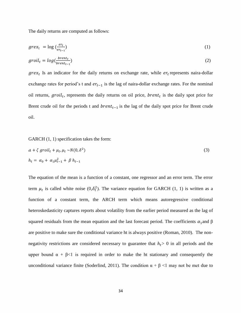
The daily returns are computed as follows:

(1)

(2)

Is an indicator for the daily returns on exchange rate, while represents naira-dollar

exchange rates for period’s t and is the lag of naira-dollar exchange rates. For the nominal

oil returns, , represents the daily returns on oil price, is the daily spot price for

Brent crude oil for the periods t and is the lag of the daily spot price for Brent crude

oil.

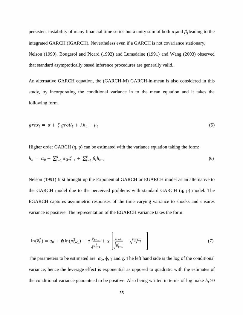
GARCH (1, 1) specification takes the form:

(3)

The equation of the mean is a function of a constant, one regressor and an error term. The error

term is called white noise (0, ). The variance equation for GARCH (1, 1) is written as a

function of a constant term, the ARCH term which means autoregressive conditional

heteroskedasticity captures reports about volatility from the earlier period measured as the lag of

squared residuals from the mean equation and the last forecast period. The coefficients and β

are positive to make sure the conditional variance ht is always positive (Roman, 2010). The non-

negativity restrictions are considered necessary to guarantee that > 0 in all periods and the

upper bound α + β<1 is required in order to make the ht stationary and consequently the

unconditional variance finite (Soderlind, 2011). The condition α + β <1 may not be met due to

35

persistent instability of many financial time series but a unity sum of both and leading to the

integrated GARCH (IGARCH). Nevertheless even if a GARCH is not covariance stationary,

Nelson (1990), Bougerol and Picard (1992) and Lumsdaine (1991) and Wang (2003) observed

that standard asymptotically based inference procedures are generally valid.

An alternative GARCH equation, the (GARCH-M) GARCH-in-mean is also considered in this

study, by incorporating the conditional variance in to the mean equation and it takes the

following form.

(5)

Higher order GARCH (q, p) can be estimated with the variance equation taking the form:

(6)

Nelson (1991) first brought up the Exponential GARCH or EGARCH model as an alternative to

the GARCH model due to the perceived problems with standard GARCH (q, p) model. The

EGARCH captures asymmetric responses of the time varying variance to shocks and ensures

variance is positive. The representation of the EGARCH variance takes the form:

α

(7)

The parameters to be estimated are , ϕ, and χ. The left hand side is the log of the conditional

variance; hence the leverage effect is exponential as opposed to quadratic with the estimates of

the conditional variance guaranteed to be positive. Also being written in terms of log make >0

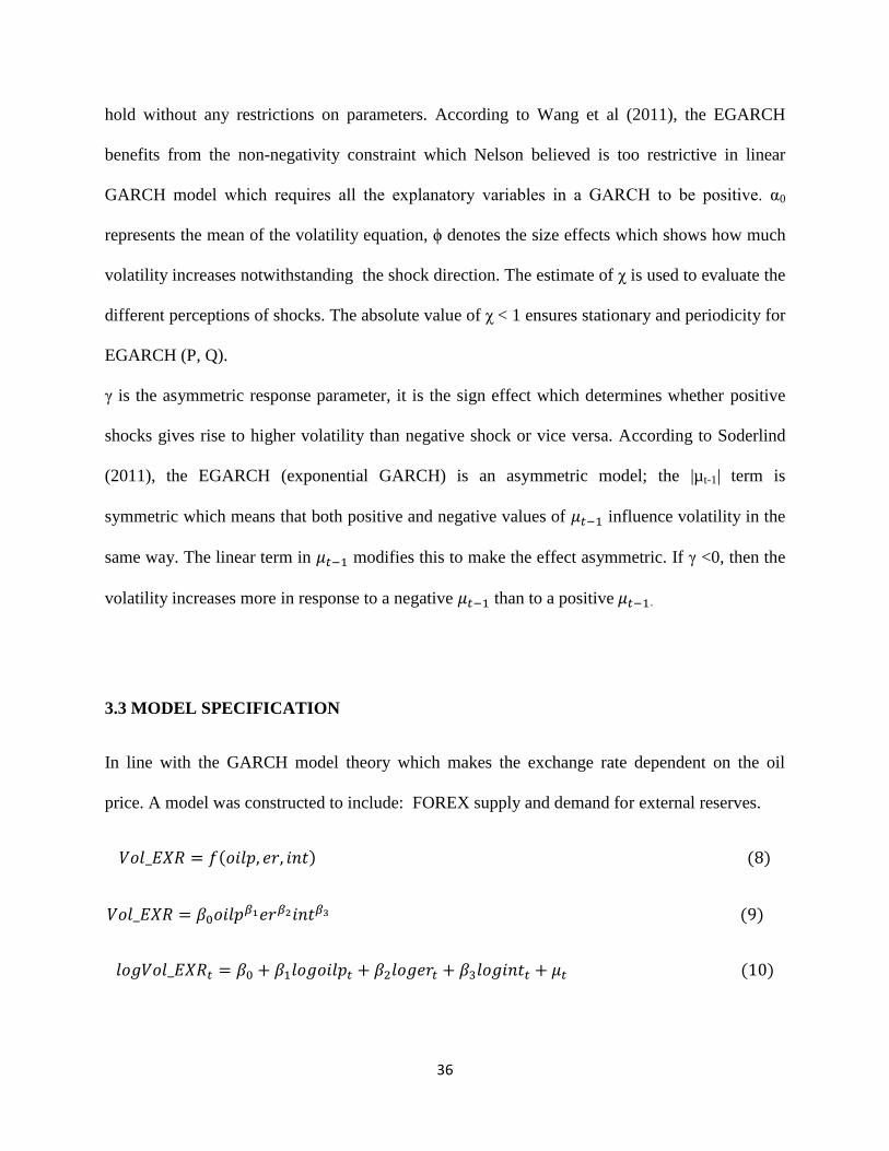
36

hold without any restrictions on parameters. According to Wang et al (2011), the EGARCH

benefits from the non-negativity constraint which Nelson believed is too restrictive in linear

GARCH model which requires all the explanatory variables in a GARCH to be positive. α0

represents the mean of the volatility equation, ϕ denotes the size effects which shows how much

volatility increases notwithstanding the shock direction. The estimate of χ is used to evaluate the

different perceptions of shocks. The absolute value of χ < 1 ensures stationary and periodicity for

EGARCH (P, Q).

is the asymmetric response parameter, it is the sign effect which determines whether positive

shocks gives rise to higher volatility than negative shock or vice versa. According to Soderlind

(2011), the EGARCH (exponential GARCH) is an asymmetric model; the |µt-1| term is

symmetric which means that both positive and negative values of influence volatility in the

same way. The linear term in modifies this to make the effect asymmetric. If <0, then the

volatility increases more in response to a negative than to a positive .

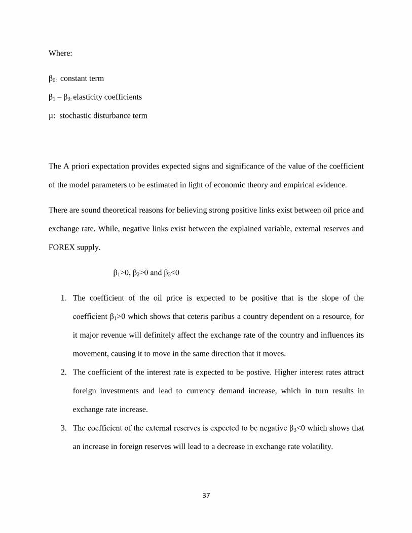
3.3 MODEL SPECIFICATION

In line with the GARCH model theory which makes the exchange rate dependent on the oil

price. A model was constructed to include: FOREX supply and demand for external reserves.

37

Where:

β0: constant term

β1 – β3: elasticity coefficients

µ: stochastic disturbance term

The A priori expectation provides expected signs and significance of the value of the coefficient

of the model parameters to be estimated in light of economic theory and empirical evidence.

There are sound theoretical reasons for believing strong positive links exist between oil price and

exchange rate. While, negative links exist between the explained variable, external reserves and

FOREX supply.

β1>0, β2>0 and β3<0

1. The coefficient of the oil price is expected to be positive that is the slope of the

coefficient β1>0 which shows that ceteris paribus a country dependent on a resource, for

it major revenue will definitely affect the exchange rate of the country and influences its

movement, causing it to move in the same direction that it moves.

2. The coefficient of the interest rate is expected to be postive. Higher interest rates attract

foreign investments and lead to currency demand increase, which in turn results in

exchange rate increase.

3. The coefficient of the external reserves is expected to be negative β3<0 which shows that

an increase in foreign reserves will lead to a decrease in exchange rate volatility.

38

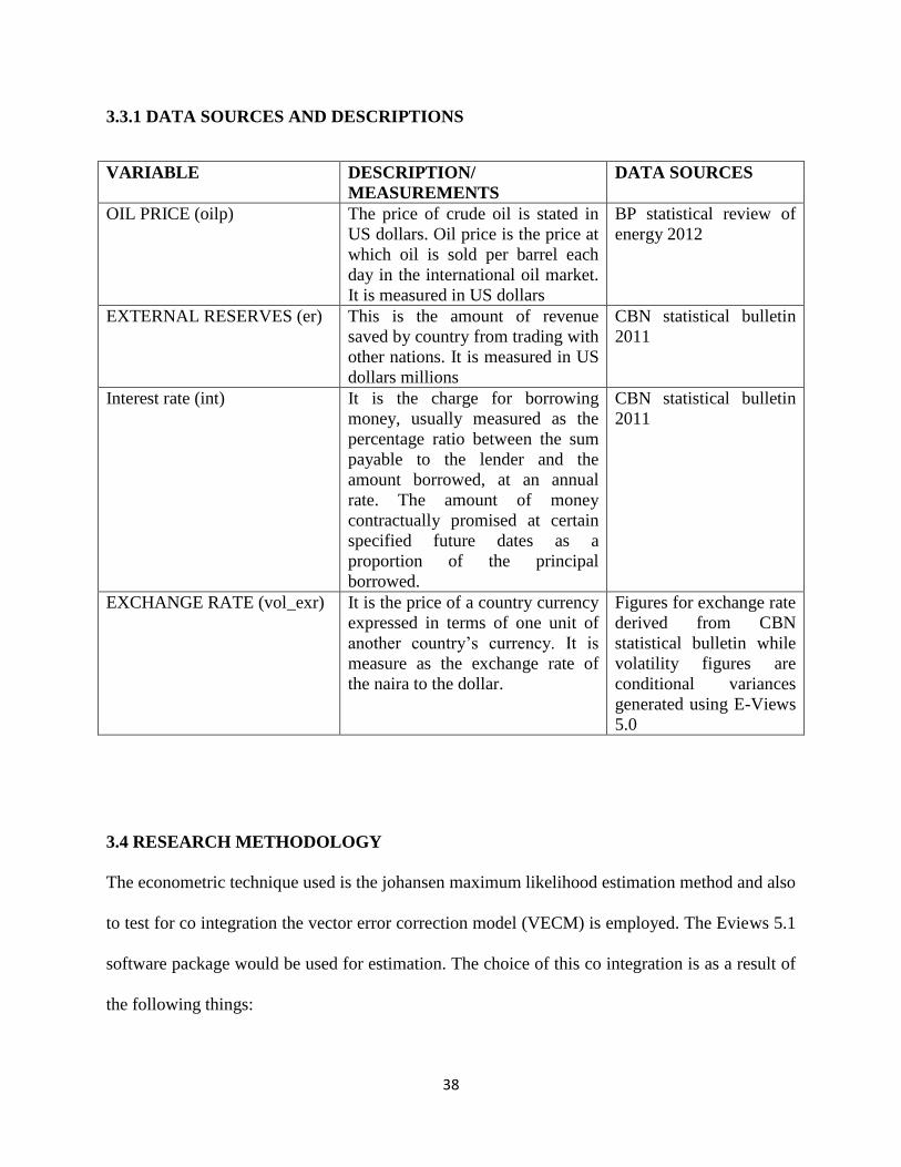
3.3.1 DATA SOURCES AND DESCRIPTIONS

VARIABLE DESCRIPTION/

MEASUREMENTS

DATA SOURCES

OIL PRICE (oilp) The price of crude oil is stated in

US dollars. Oil price is the price at

which oil is sold per barrel each

day in the international oil market.

It is measured in US dollars

BP statistical review of

energy 2012

EXTERNAL RESERVES (er) This is the amount of revenue

saved by country from trading with

other nations. It is measured in US

dollars millions

CBN statistical bulletin

2011

Interest rate (int) It is the charge for borrowing

money, usually measured as the

percentage ratio between the sum

payable to the lender and the

amount borrowed, at an annual

rate. The amount of money

contractually promised at certain

specified future dates as a

proportion of the principal

borrowed.

CBN statistical bulletin

2011

EXCHANGE RATE (vol_exr) It is the price of a country currency

expressed in terms of one unit of

another country’s currency. It is

measure as the exchange rate of

the naira to the dollar.

Figures for exchange rate

derived from CBN

statistical bulletin while

volatility figures are

conditional variances

generated using E-Views

5.0

3.4 RESEARCH METHODOLOGY

The econometric technique used is the johansen maximum likelihood estimation method and also

to test for co integration the vector error correction model (VECM) is employed. The Eviews 5.1

software package would be used for estimation. The choice of this co integration is as a result of

the following things:

39

1. Most time series data are not stationary that is they do not have a constant mean, a

constant variance and a constant auto variance for every successive lag) so the use of the

OLS method of estimation would only yield unauthentic results.

2. Co integration view is a convenient approach for the estimation of long run parameters

with unit root.

3. The co integration approach provides a direct test of the economic theory and enables

utilization of the estimated long run parameters into the estimation of the short run

disequilibrium relationships

4. The traditional approach is criticized for ignoring the problems caused by the presence of

unit roots variables in the data generating process. However both unit root and co

integration have important implications for the specification and estimation of dynamic

models

UNIT ROOT TEST OR THE TEST FOR STATIONARITY

The unit root test is carried out before the co integration method of analyses can be carried out;

this is because it is necessary to test for the presence of a unit root in a variable. A unit root test

tests whether time series variable is non-stationary using autoregressive model. A test that is very

popular and valid for large samples is the Augmented dickey fuller (ADF) and another test that

can be used is Phillips Perron test. They are used to determine the order of integration of a

variable.

The test states that if a particular series say Y has to be differenced n times (number of times, 1,

2, 3… n) before it becomes stationary then Y is said to be integrated of order n ( it is written as

I(n) ). If the series is stationary at level it is said to be integrated to order 0 (I(0)), that is there is

40

no unit root. If a variable is differentiated once in order for it to be stationary it is said to be

integrated to order 1 that is I(1).

The test statistics of the estimated coefficient of Yt is then used to test the null hypothesis that

the series is non-stationary (has unit root). If the absolute value of the test statistics is higher than

the absolute value of the critical T value (which could be at 1, 5, or 10 percent) then he series is

said to be stationary, therefore we reject the null hypothesis, otherwise it has to be differentiated

until is stationary.

JOHANSEN TEST FOR COINTEGRATION

Co integration is basically based on the idea that there is a long run co movement between

trended economic time series so that there is a common equilibrium relation which the time

series have a tendency to revert to, therefore even if certain time series, they are non-stationary, a

linear combination of them may exist that is stationary

A lot of economic series behave like I(1) processes that is they seem to drift all over the place,

but another thing to notice is that they seem to drift in such a way that they do not drift away

from each other. Formulating it statistically you will come up with a co integration model.

Johansen test named after Soren Johansen, is procedure, is a procedure for testing co integration

of several I (1) time series. This test permits more than one co integrating relationships, so it’s

more applicable than the Engle-Granger test which is OLS based. There are two types of

Johansen test, Trace and Maximal Eigen value which are used to test for co integration and they

are also used to determine the number of co integrating vectors. Both tests do not always indicate

the same number of co integrating vectors. The trace test is a joint test, the null hypothesis is that

the number of co integrating vectors is less than or equal to r against a general alternative

41

hypothesis that there are more than r. the Maximal Eigen value test conducts separate test on

each Eigen value. The null hypothesis is that r co integrating vectors present against the

alternative that there are (r+1) present. If there are g variables in the system of equations, there

can be a maximum of g-1 co integrating vectors.

ADVANTAGES OF THE USE OF JOHANSEN TECHNIQUE

1. The core benefit of Johansen Vector Autoregressive estimation procedure in the testing

and estimation of the numerous long-run equilibrium relationship.

2. It allows testing of various economic hypotheses via linear restrictions in co integration

space is possible when using johansen estimation method.

CRITICISMS OF THE JOHANSEN TECHNIQUE

1. The result can be sensitive to the number of lags included in the test and the presence of

autocorrelation

2. Higher requirements in Johansen’s estimation method for the number of observations

than the Engle-granger procedure usually necessitates, the use of quarterly or monthly

time series data, which are not always readily available.

3. If the two test statistics differ, which one gives the correct results?

4. Problems identifying (multiple) co integration vectors with theoretical economic

relationships are possible using Johansen method.

HOW TO OVER COME THE WEAKNESS

1. By identifying co integrating vectors, if the model is consistent with economic theory, it

should consist of two or more single equations.

42

2. The problem can be corrected by a lag length test which would estimate vector auto-

regression using undifferentiated data.

THE VECTOR ERROR CORRECTION MODEL

This is basic VAR, with an error correction term incorporated into the model. The reason for the

error correction term is the same as with the standard error correction model, it measures any

movements away from the long run equilibrium and measures the speed of adjustment of the

short run dynamics to the long run equilibrium time path. The coefficient is expected to be

negatively signed. The vector error correction model would be used to analyze the short run

relationship between the world crude oil price and the Nigerian exchange rate.

GARCH (1,1) MODEL

The exchange rate volatility aspect of the model is estimated using the GARCH (1,1) model of

estimation. It is believed that the GARCH model can generate good estimates of exchange rate

volatility (Egwaikhide and Udoh, 2008)

The GARCH model was developed independently by Bollerslev (1986) and Taylor (1986). It is

used by several professionals in several areas including, trading, investing, hedging and dealing.

The process for GARCH model involves three steps: estimate the best fitting autoregressive

model, compute autocorrelations of the error term and lastly test for significance. GARCH

method presumably captures risk in each period more sensibly than simply rolling standard

deviations which gives equal weights to correlated shocks and single outliners. Development of

43

the model is premised on two different specifications. There is one for the conditional mean and

another for the conditional variance (Onwusor, 2007).

The GARCH model allows the conditional variance to be dependent upon pervious own lags, so

that the conditional variance in the case is:

is known as the conditional variance. Since it is one period ahead estimate for the variance

calculated is based on any past information thought relevant.

Adapting GARCH model used by Papertrou to model oil price volatility, the mean equation of

the GARCH model is specified as:

In the mean equation, ∆LEX represents the rate of increase in the exchange rate expressed as the

difference of the logarithm of the exchange rates; and is a random error that is Gaussian in

nature implying that the error term is dependent upon itself.

The exchange rate that is used is sourced from the CBN website and the GARCH model is used

to generate the conditional variance series that is subsequently used as the exchange rate

volatility time series data from 1980 to 2011

44

CHAPTER FOUR

DATA ANALYSIS AND INTERPRETATION

4.1 Introduction

In the previous chapter a model was specified to find out the effect of oil price on exchange rate

volatility in Nigeria. This chapter focuses on the presentation, analysis and interpretation of data.

To this end the chapter is divided into two main sections:

1. Descriptive analysis

2. Econometric analysis

The descriptive analysis helps us ascertain the trend of relationship among the variables

employed in this study; most importantly, the pattern of relationship between exchange rate

volatility and sits determinants.

The econometric analysis would help us achieve the objective of finding if oil price influences

exchange rate volatility in Nigeria. Therefore the econometric analysis would investigate the

short run and long run effects of oil price on exchange rate volatility.

45

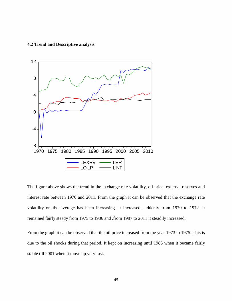
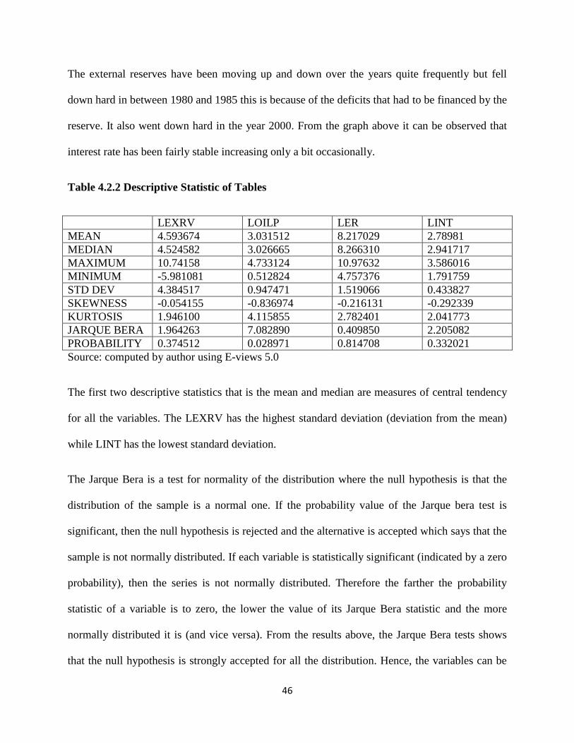
4.2 Trend and Descriptive analysis

The figure above shows the trend in the exchange rate volatility, oil price, external reserves and

interest rate between 1970 and 2011. From the graph it can be observed that the exchange rate

volatility on the average has been increasing. It increased suddenly from 1970 to 1972. It

remained fairly steady from 1975 to 1986 and .from 1987 to 2011 it steadily increased.

From the graph it can be observed that the oil price increased from the year 1973 to 1975. This is

due to the oil shocks during that period. It kept on increasing until 1985 when it became fairly

stable till 2001 when it move up very fast.

-8

-4

0

4

8

12

1970 1975 1980 1985 1990 1995 2000 2005 2010

LEXRVLOILP

LERLINT

46

The external reserves have been moving up and down over the years quite frequently but fell

down hard in between 1980 and 1985 this is because of the deficits that had to be financed by the

reserve. It also went down hard in the year 2000. From the graph above it can be observed that

interest rate has been fairly stable increasing only a bit occasionally.

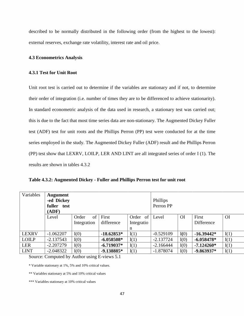
Table 4.2.2 Descriptive Statistic of Tables

LEXRV LOILP LER LINT

MEAN 4.593674 3.031512 8.217029 2.78981

MEDIAN 4.524582 3.026665 8.266310 2.941717

MAXIMUM 10.74158 4.733124 10.97632 3.586016

MINIMUM -5.981081 0.512824 4.757376 1.791759

STD DEV 4.384517 0.947471 1.519066 0.433827

SKEWNESS -0.054155 -0.836974 -0.216131 -0.292339

KURTOSIS 1.946100 4.115855 2.782401 2.041773

JARQUE BERA 1.964263 7.082890 0.409850 2.205082

PROBABILITY 0.374512 0.028971 0.814708 0.332021

Source: computed by author using E-views 5.0

The first two descriptive statistics that is the mean and median are measures of central tendency

for all the variables. The LEXRV has the highest standard deviation (deviation from the mean)

while LINT has the lowest standard deviation.

The Jarque Bera is a test for normality of the distribution where the null hypothesis is that the

distribution of the sample is a normal one. If the probability value of the Jarque bera test is

significant, then the null hypothesis is rejected and the alternative is accepted which says that the

sample is not normally distributed. If each variable is statistically significant (indicated by a zero

probability), then the series is not normally distributed. Therefore the farther the probability

statistic of a variable is to zero, the lower the value of its Jarque Bera statistic and the more

normally distributed it is (and vice versa). From the results above, the Jarque Bera tests shows

that the null hypothesis is strongly accepted for all the distribution. Hence, the variables can be

47

described to be normally distributed in the following order (from the highest to the lowest):

external reserves, exchange rate volatility, interest rate and oil price.

4.3 Econometrics Analysis

4.3.1 Test for Unit Root

Unit root test is carried out to determine if the variables are stationary and if not, to determine

their order of integration (i.e. number of times they are to be differenced to achieve stationarity).

In standard econometric analysis of the data used in research, a stationary test was carried out;

this is due to the fact that most time series data are non-stationary. The Augmented Dickey Fuller

test (ADF) test for unit roots and the Phillips Perron (PP) test were conducted for at the time

series employed in the study. The Augmented Dickey Fuller (ADF) result and the Phillips Perron

(PP) test show that LEXRV, LOILP, LER AND LINT are all integrated series of order I (1). The

results are shown in tables 4.3.2

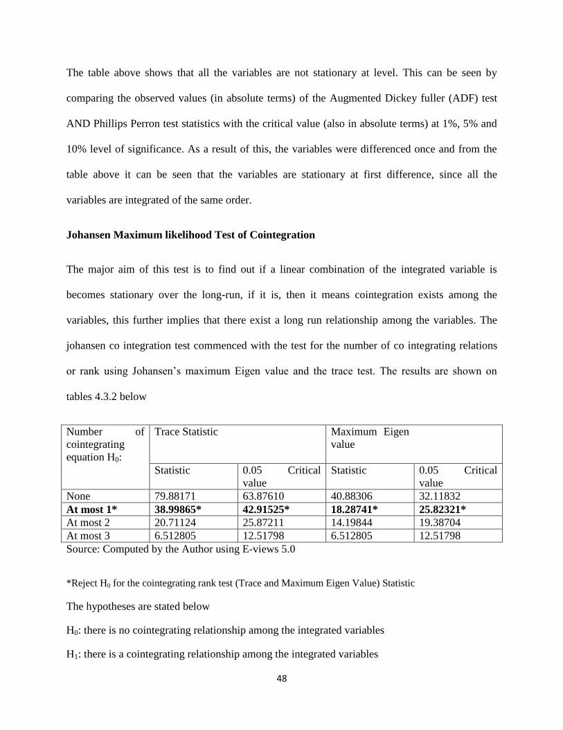
Table 4.3.2: Augmented Dickey - Fuller and Phillips Perron test for unit root

Variables Augument

-ed Dickey

fuller test

(ADF)

Phillips

Perron PP

Level Order of

Integration

First

difference

Order of

Integratio

n

Level OI First

Difference

OI

LEXRV -1.062207 I(0) -18.62853* I(1) -0.529109 I(0) -16.39442* I(1)

LOILP -2.137543 I(0) -6.058508* I(1) -2.137724 I(0) -6.058478* I(1)

LER -2.207279 I(0) -6.719037* I(1) -2.166444 I(0) -7.124260* I(1)

LINT -2.048322 I(0) -9.138885* I(1) -1.878074 I(0) -9.863937* I(1)

Source: Computed by Author using E-views 5.1

* Variable stationary at 1%, 5% and 10% critical values.

** Variables stationary at 5% and 10% critical values

*** Variables stationary at 10% critical values

48

The table above shows that all the variables are not stationary at level. This can be seen by

comparing the observed values (in absolute terms) of the Augmented Dickey fuller (ADF) test

AND Phillips Perron test statistics with the critical value (also in absolute terms) at 1%, 5% and

10% level of significance. As a result of this, the variables were differenced once and from the

table above it can be seen that the variables are stationary at first difference, since all the

variables are integrated of the same order.

Johansen Maximum likelihood Test of Cointegration

The major aim of this test is to find out if a linear combination of the integrated variable is

becomes stationary over the long-run, if it is, then it means cointegration exists among the

variables, this further implies that there exist a long run relationship among the variables. The

johansen co integration test commenced with the test for the number of co integrating relations

or rank using Johansen’s maximum Eigen value and the trace test. The results are shown on

tables 4.3.2 below

Number of

cointegrating

equation H0:

Trace Statistic Maximum Eigen

value

Statistic 0.05 Critical

value

Statistic 0.05 Critical

value

None 79.88171 63.87610 40.88306 32.11832

At most 1* 38.99865* 42.91525* 18.28741* 25.82321*

At most 2 20.71124 25.87211 14.19844 19.38704

At most 3 6.512805 12.51798 6.512805 12.51798

Source: Computed by the Author using E-views 5.0

*Reject H0 for the cointegrating rank test (Trace and Maximum Eigen Value) Statistic

The hypotheses are stated below

H0: there is no cointegrating relationship among the integrated variables

H1: there is a cointegrating relationship among the integrated variables

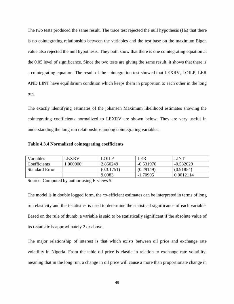
49

The two tests produced the same result. The trace test rejected the null hypothesis (H0) that there

is no cointegrating relationship between the variables and the test base on the maximum Eigen

value also rejected the null hypothesis. They both show that there is one cointegrating equation at

the 0.05 level of significance. Since the two tests are giving the same result, it shows that there is

a cointegrating equation. The result of the cointegration test showed that LEXRV, LOILP, LER

AND LINT have equilibrium condition which keeps them in proportion to each other in the long

run.

The exactly identifying estimates of the johansen Maximum likelihood estimates showing the

cointegrating coefficients normalized to LEXRV are shown below. They are very useful in

understanding the long run relationships among cointegrating variables.

Table 4.3.4 Normalized cointegrating coefficients

Variables LEXRV LOILP LER LINT

Coefficients 1.000000 2.860249 -0.531970 -0.532029

Standard Error (0.3.1751) (0.29149) (0.91854)

9.0083 -1.70905 0.0012114

Source: Computed by author using E-views 5.

The model is in double logged form, the co-efficient estimates can be interpreted in terms of long

run elasticity and the t-statistics is used to determine the statistical significance of each variable.

Based on the rule of thumb, a variable is said to be statistically significant if the absolute value of

its t-statistic is approximately 2 or above.

The major relationship of interest is that which exists between oil price and exchange rate

volatility in Nigeria. From the table oil price is elastic in relation to exchange rate volatility,

meaning that in the long run, a change in oil price will cause a more than proportionate change in

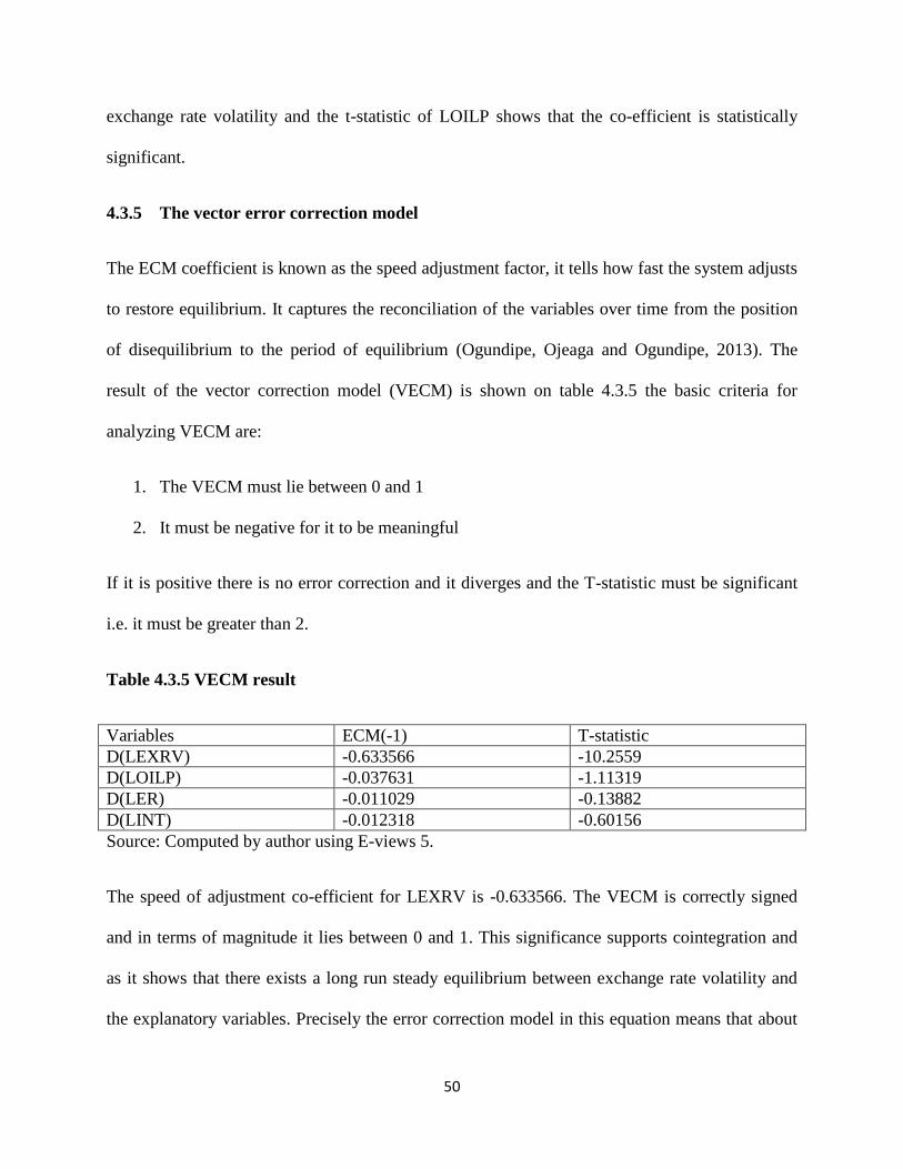
50

exchange rate volatility and the t-statistic of LOILP shows that the co-efficient is statistically

significant.

4.3.5 The vector error correction model

The ECM coefficient is known as the speed adjustment factor, it tells how fast the system adjusts

to restore equilibrium. It captures the reconciliation of the variables over time from the position

of disequilibrium to the period of equilibrium (Ogundipe, Ojeaga and Ogundipe, 2013). The

result of the vector correction model (VECM) is shown on table 4.3.5 the basic criteria for

analyzing VECM are:

1. The VECM must lie between 0 and 1

2. It must be negative for it to be meaningful

If it is positive there is no error correction and it diverges and the T-statistic must be significant

i.e. it must be greater than 2.

Table 4.3.5 VECM result

Variables ECM(-1) T-statistic

D(LEXRV) -0.633566 -10.2559

D(LOILP) -0.037631 -1.11319

D(LER) -0.011029 -0.13882

D(LINT) -0.012318 -0.60156

Source: Computed by author using E-views 5.

The speed of adjustment co-efficient for LEXRV is -0.633566. The VECM is correctly signed

and in terms of magnitude it lies between 0 and 1. This significance supports cointegration and

as it shows that there exists a long run steady equilibrium between exchange rate volatility and

the explanatory variables. Precisely the error correction model in this equation means that about

51

63.35% of errors generated between each period are correlated in subsequent periods. This result

is sizeable and also significant judging from the value of the T-statistic [-10.2559].

4.4 Findings and Economic interpretation

The study was carried out majorly to determine the effects of oil price on exchange rate volatility

in Nigeria. The result obtained is in line with the expectation of the study. It showed that a

proportionate change in oil price leads to a more than proportionate change in exchange rate

volatility by 2.86. This indicates a change in international oil price will have a greater effect than

expected on exchange rate volatility in Nigeria. In the long run the coefficient of elasticity of

2.8% implies that exchange rate volatility is elastic to changes in the oil price since the

coefficient is greater than one. It is statistically significant based on the t-statistic.

Crude oil is the mainstay of Nigeria’s economy. It affects all her economic activities and

influences are macroeconomic variable including exchange rate.

The result obtained showed that a proportionate change in external reserves leads to a less than

proportionate change in exchange rate volatility. This is in line with the expectation of the study.

This means that a change in external reserves for Nigeria will have less than the expected change

in exchange rate volatility in Nigeria. In the long run the coefficient of elasticity of 0.53%

implies that exchange rate volatility is inelastic to changes in the exchange rate volatility since

the coefficient is less than one. Based on the rule of thumb that a variable is said to be

statistically significant if the absolute value of the t-statistic is approximately 2 or above, that

means a significant relationship exist between external reserves and exchange rate volatility.

52

According to Ketil (2004) a reasonable level of external reserves is sufficient to reduce a

country’s exchange rate volatility. Nigeria’s external reserves increases when oil revenue

increase and this eternal reserves can be used to reduce exchange rate volatility

A proportionate change in oil price leads to a less than proportionate change in interest rate. This

is not in line with the expectation of the study. This means that a change in Nigeria’s interest rate

will have a smaller effect than expected on exchange rate volatility. In the long run the

coefficient of elasticity of 0.53% implies that exchange rate volatility is inelastic to changes in

Nigeria’s interest rate since the coefficient is less than one. This implies that a change in

Nigeria’s interest rate will not have a significant impact on exchange rate volatility in Nigeria

and it is not statistically significant looking at the t-statistic.

When a country’s interest rate is high, it attracts investment from abroad which increases its

exchange rate but when inflation in the country is high like in Nigeria, it mitigates the influence

of interest rate on exchange rate.

4.5 Conclusion

This chapter focused on the analysis and the interpretation of data. The chapter started with the

descriptive analysis of the variables next was the analysis of the data which included unit root

tests on the variables to be used in the study. The Augmented Dickey Fuller (ADF) and the

Phillips Perron (PP) tests were used to find out if the variables were stationary and to what

degree. The variables where then found to be stationary at first difference, then the johansen test

of cointegration was performed on the integrated variables, they were found to be cointegrated

and so the normalized coefficient were then reported. The result of oil price, external reserves

and interest rate did not follow the a priori expectations and the probable reasons were given

53

looking at the Nigerian situation. The Vector Error Correction Model (VECM) was employed to

reconcile the short run deviations to the long run equilibrium path. The ECM(-1) coefficient of

the vector of concern (DLEXRV) was rightly signed. The result appeared sizeable judging from

the value of the T-statistic. Therefore the alternative hypothesis that oil price has a significant

influence on exchange rate volatility should be accepted.

54

CHAPTER FIVE

SUMMARY, RECOMMENDATION AND CONCLUSION

5.1 SUMMARY

This research study set to find out if oil price as a significant influence on exchange rate

volatility in Nigeria over the periods 1970 -2010 by analyzing time series data. It also looks at

other factors that can influence exchange rate in Nigeria like external reserves and interest rate.

To achieve these objectives, a model was formulated based on GARCH model. In the model

exchange rate volatility was the dependent variable and the independent variables were oil price,

external reserves and interest rate. After the review of relevant literature and the necessary

empirical analyses it was observed that a proportionate change in oil price will lead to a more

than proportionate change in exchange rate volatility.

5.2 POLICY RECOMMENDADATIONS

In the words of Jin (2008), Exchange rate volatility increases the risk and uncertainty of external

transactions and predisposes a country to exchange rate related risks. For the purpose of this

research work, the following strategies are suggested to reduce exchange rate volatility in

Nigeria.

1. Ketil (2004) research on the effect of external reserves on exchange rate volatility after

enforcing controls for the endogeneity induced by the exchange rate regime that can

affect both reserves and exchange rate showed that a high level of external reserves

reduce exchange rate volatility. Therefore Nigeria government should take advantage of

55

increases in the price of oil price by Nigeria external reserves and reduce exchange rate

volatility.

2. Research carried out on exchange rate volatility by Adeoye and Atanda showed that there

is presence and persistency of volatility shocks in the nominal and real exchange rates for

naira vis-à-vis U.S dollar in Nigeria between 1986 and 2008. This implies that the

conservative monetary management policies put in place for stabilizing the exchange rate

of a unit U.S dollar to naira over the years has been ineffective. There is a need for

FOREX management measures particularly in terms of meeting the high demand for

foreign currency which characterized and order the performance and trade balance and

overall economic performance in Nigeria. There is also the need for sound monetary

policy to attain stability in the exchange rate.

3. According to the Brahmbhatt et al (2010), resources that a gift by God to a country prices

and revenues are a lot unpredictable because of the small diminutive supply elasticity of

natural resource yield. Assuming government expenditure is closely aligned to revenue

from natural resource, the revenue will become more unpredictable. Expenditure

instability, will in turn cause instability in the real exchange rate. A bulky body of

empirical work records the terrible effect of the impact of economic volatility on

investment and growth. Therefore Nigeria government should look for new ways to

diversify the economy from dependence on oil and explore other sectors like

manufacturing sector and agricultural sector to reduce volatility in the economy and the

overall effect on it.

56

4. Lastly, higher revenue gotten from increases in oil prices should be invested different

areas of the economy the economy as the exchange rate of a country is affected by state

of the economy.

5.3 LIMITATIONS TO THE STUDY

The limitations of this study were mostly data related. I originally wanted to use FOREX supply

as one of the independent variable but the data available was only from the year 1996 to 2011.

Another limitation was error in estimation a characteristic of secondary data.

5.4 SUGGESTIONS FOR FURTHER STUDY

An interesting variant to this study would be an in-depth review of past approaches to controlling

or reducing exchange rate volatility in countries that have Dutch disease and lessons that can be

learnt to develop strategies and approaches that will reduce exchange rate volatility in Nigeria.

5.5 CONCLUSION

This research project looked at oil price in Nigeria and its effect on exchange rate volatility in

Nigeria. The policy discussed and recommended if carried out will help Nigeria take advantage

of increases in oil price and the help reduce exchange rate volatility which in turn will improve

economic growth in Nigeria.

57

REFERENCES

Adedipe, B. (2004). The Impact of Oil on Nigeria’s Economic Policy formulation. Maximizing

Pro-poor Growth: Regenerating the Socio-economic Database, organized by

Overseas Development Institute in collaboration with the Nigerian Economic Summit

Group, 16th -17th June 2004

Adeniyi, O.A. (2011). Oil price shocks and Exchange rate dynamics in oil exporting countries:

what is the Nigerian experience? Being a paper presented at the Fourth

NAEE/IAEE international Conference

Adeniyi, O., Omisakan, O., Yaqub, J. & Oyinlola, A. (2012). Oil price-Exchange rate Nexus in

Nigeria: Further Evidence from an oil exporting country.

Adeoye, B. W. & Atanda, A.A. Exchnage rate Volatility in Nigeria consistency, Persistency and

Severity Analyses, CBN Journal of Applied Statistics Vol.2 No.2

Akram, Q. F. (2004). Oil prices and exchange rates: Norwegian evidence, The Econometrics

Journal, 7, pp. 476–504

AL-Ezzee, I. (2011). Real influences of Real Exchange rate and Oil price changes on the growth

of real GDP: Case of Bahrain, International Conference of Management and service

science IPEDR vol.8

Aliyu, S., & Usman, R. (2009a). Impact of Oil Price Shock and Exchange Rate Volatility on

Economic Growth in Nigeria: An Empirical Investigation, Journal of International

Studies Issue 11, pp4-15

Amano, R., & Norden, S. (1995). Exchange Rate and Oil Price, Bank of Canada working Paper

no.95-8.

58

Bagella, M., Becchetti, L., Hasan, I. (2006) Real effective exchange rate volatility and growth:

A framework to measure advantages of flexibility vs. costs of volatility, J. Bank Finance

30 (2006) 1149-169.

Beckmann, J., & Czudaj, R. (2012) Oil price and U.s dollar exchange rate dynamics

Bollerslev, T., (1986) Generalised Autoregressive Conditional Heteroskedasticity, Journal of

Econometrics 31, 307–327

Brahmbhatt, M., Canuto, O., & Vostroknutova, E. (2010). Dealing With Dutch disease, poverty

and economic management network (PREM), No. 16,June, pp4

Cashin, P., Céspedes, L. F; & Sahay, R. (2004) “Commodity currencies and the real exchange

rate,” Journal of Development Economics, Vol. 75, 239–268.

Chen, H., & Chen, C., (2007). Oil Prices and Real Exchange Rate, Energy Economics, 29, 390–

404

Dawson, J. (2010). The effect of Oil price on Exchange rate in Nigeria: The case of Dominican

republic.

Englama, A., Duke, O. O., Ogunleye, S., & Isma F. U. (2010). Oil Price and Exchange rate

Volatility in Nigeria: An Empirical observation.

Engle, R. F (1982). Autoregressive Conditiional Heteroscedasticity with Estimates of the

Variance of United Kingdom Inflation. Econometrica, 50, pp987-1007.

Habib, M. M; &Kalamova, M. (2007). Are There Oil Currencies? The Real Exchange Rate of

Oil Exporting Countries, In European Central Bank working Paper 839.

Isard, P. (2007) “Equilibrium Exchange Rates: Assessment Methodologies” IMF Working paper

WP/07/296

Jin, G., (2008) The Impact of Oil Price Shock and Exchange Rate Volatility on Economic

59

Growth: A comparative analysis for Russia, Japan, and China. Research Journal of

International Studies, Issue 8, pp98-111

Koranchelian, T., (2005): “The Equilibrium Real Exchange Rate in a Commodity Exporting

Country”: Algeria‟s Experience, IMF Working Paper 05/135

Korhonen, I. and T. Juurikkala (2007): "Equilibrium exchange rates in oil-dependent

countries," BOFIT Discussion Papers 8/2007, Bank of Finland, Institute for

Economies in Transition

Krugman, P., (1983). Oil shocks and exchange rate dynamics In Exchange Rates and

International Macroeconomics, University of Chicago Press

McKillop, A. (2004) “Oil Prices, Economic Growth and World Oil Demand”,

Middle East

Economic Survey, vol. xlvii No 35.

Mordi, C. N. O. (2006). Challenges of Exchange Rate Volatility in Economic Management in

Nigeria. Central Bank of Nigeria Bullion, 30(3).

Muhammad, Z., Suleiman, H., & Kouhy, R. (2010). Exploring Oil Price-Exchange rate nexus

for Nigeria. FIW working paper No71

Nelson, D. B. (1991). Conditional heteroscedasticity in asset returns: a new approach.

Econometrica, 59, pp347−370.

Obadan, M. I. (2006). Overview of Exchange rate Management in Nigeria from 1986 to date.

CBN statistical bulletin, vol, No. 3 (July-September)

Odularu, G.O. (2007). Crude Oil and Nigeria Economic Performance

Ojebiyi, A. & Wilson D. O. (2011). Exchange rate Volatility: An analysis of the relationship

60

between Naira, Oil price and US dollars

Ogundipe A.A and Ogundipe O.M (2013). Oil Price and Exchange Rate Volatility in Nigeria.

MPRA Working Paper

Ogundipe A.A, Ojeaga P, and Ogundipe O.M, (2013). Estimating the Long-run Effect of

Exchange Rate Devaluation on the trade balance in Nigeria. European Scientific Journal

vol. 9 No. 25

Olomola, A., (2006): “Oil Price Shock and Aggregate Economic Activity in Nigeria”, African

Economic and Business Review Vol.4: 2, ISSN 1109-5609

Olomola, P.A., Adejumo A.V. (2006). Oil Price Shocks and Macroeconomic Activities in

Nigeria, International Research Journal of Finance and Economics, 3, 28–34.

Plante, M. (2008). Oil price shocks and Exchange rate management: the implications of

consumer durables for the small open economy

Ricken J. (2009): “Oil Price and Real Exchange Rate Volatility in Oil-Exporting Economies: The

Role of Governance”, IFN Working paper No. 810, Research

Sanusi, J. (2004). Nigeria’s Exchange rate mechanism: The current Experience. Being a

Paper presented at Nigerian- British Chamber of commerce.

Schnabl, G. (2007). “Exchange Rate Volatility and Growth in Small Open Economies at the

EMU Periphery Working Paper Series, No. 773

Serven, L. & Solimano A. (1993). Striving for Growth after adjustment: The Role of

Capital Formation.

Spatafora, N., & Stavrev, E. (2003). The Equilibrium Real Exchange Rate in a Commodity

Exporting Country: The Case of Russia, IMF Working Paper 93

Söderlind, P. (2011). Lecture Notes in Financial Econometrics In (MBF, MSc course at

61

UNISG).University of St.Gallen. Switzerland.

Trung, V. & Vinh, N., (2011). The Impact of Oil prices, Real Effective exchange rate and

Inflation on Economic Activity: Novel Evidence for Vietnan

Umar, A. & Soliu, U. The Foreign Exchange rates in Nigeria: Convergence and Divergence

Wang, P. (2003). Financial Econometrics: Methods and Models London: Routledge

advanced texts in economics and finance.

Xavier, S. &Subramanian, A. (2003), “Addressing the Natural Resource Curse: An Illustration

from Nigeria,” NBER Working Paper 9804, Cambridge, Mass

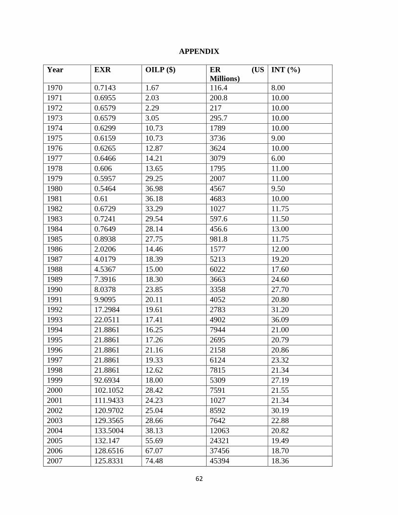
62

APPENDIX

Year EXR OILP ($) ER (US

Millions)

INT (%)

1970 0.7143 1.67 116.4 8.00

1971 0.6955 2.03 200.8 10.00

1972 0.6579 2.29 217 10.00

1973 0.6579 3.05 295.7 10.00

1974 0.6299 10.73 1789 10.00

1975 0.6159 10.73 3736 9.00

1976 0.6265 12.87 3624 10.00

1977 0.6466 14.21 3079 6.00

1978 0.606 13.65 1795 11.00

1979 0.5957 29.25 2007 11.00

1980 0.5464 36.98 4567 9.50

1981 0.61 36.18 4683 10.00

1982 0.6729 33.29 1027 11.75

1983 0.7241 29.54 597.6 11.50

1984 0.7649 28.14 456.6 13.00

1985 0.8938 27.75 981.8 11.75

1986 2.0206 14.46 1577 12.00

1987 4.0179 18.39 5213 19.20

1988 4.5367 15.00 6022 17.60

1989 7.3916 18.30 3663 24.60

1990 8.0378 23.85 3358 27.70

1991 9.9095 20.11 4052 20.80

1992 17.2984 19.61 2783 31.20

1993 22.0511 17.41 4902 36.09

1994 21.8861 16.25 7944 21.00

1995 21.8861 17.26 2695 20.79

1996 21.8861 21.16 2158 20.86

1997 21.8861 19.33 6124 23.32

1998 21.8861 12.62 7815 21.34

1999 92.6934 18.00 5309 27.19

2000 102.1052 28.42 7591 21.55

2001 111.9433 24.23 1027 21.34

2002 120.9702 25.04 8592 30.19

2003 129.3565 28.66 7642 22.88

2004 133.5004 38.13 12063 20.82

2005 132.147 55.69 24321 19.49

2006 128.6516 67.07 37456 18.70

2007 125.8331 74.48 45394 18.36

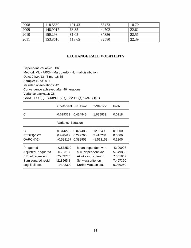
63

2008 118.5669 101.43 58473 18.70

2009 148.9017 63.35 44702 22.62

2010 150.298 81.05 37356 22.51

2011 153.8616 113.65 32580 22.39

EXCHANGE RATE VOLATILITY

Dependent Variable: EXR

Method: ML - ARCH (Marquardt) - Normal distribution

Date: 04/24/13 Time: 18:35

Sample: 1970 2011

Included observations: 42

Convergence achieved after 40 iterations

Variance backcast: ON

GARCH = C(2) + C(3)*RESID(-1)^2 + C(4)*GARCH(-1) Coefficient Std. Error z-Statistic Prob. C 0.699363 0.414845 1.685839 0.0918 Variance Equation C 0.344220 0.027485 12.52408 0.0000

RESID(-1)^2 0.998412 0.292765 3.410284 0.0006

GARCH(-1) -0.588157 0.388953 -1.512153 0.1305 R-squared -0.578519 Mean dependent var 43.90908

Adjusted R-squared -0.703139 S.D. dependent var 57.49835

S.E. of regression 75.03785 Akaike info criterion 7.301867

Sum squared resid 213965.8 Schwarz criterion 7.467360

Log likelihood -149.3392 Durbin-Watson stat 0.030250

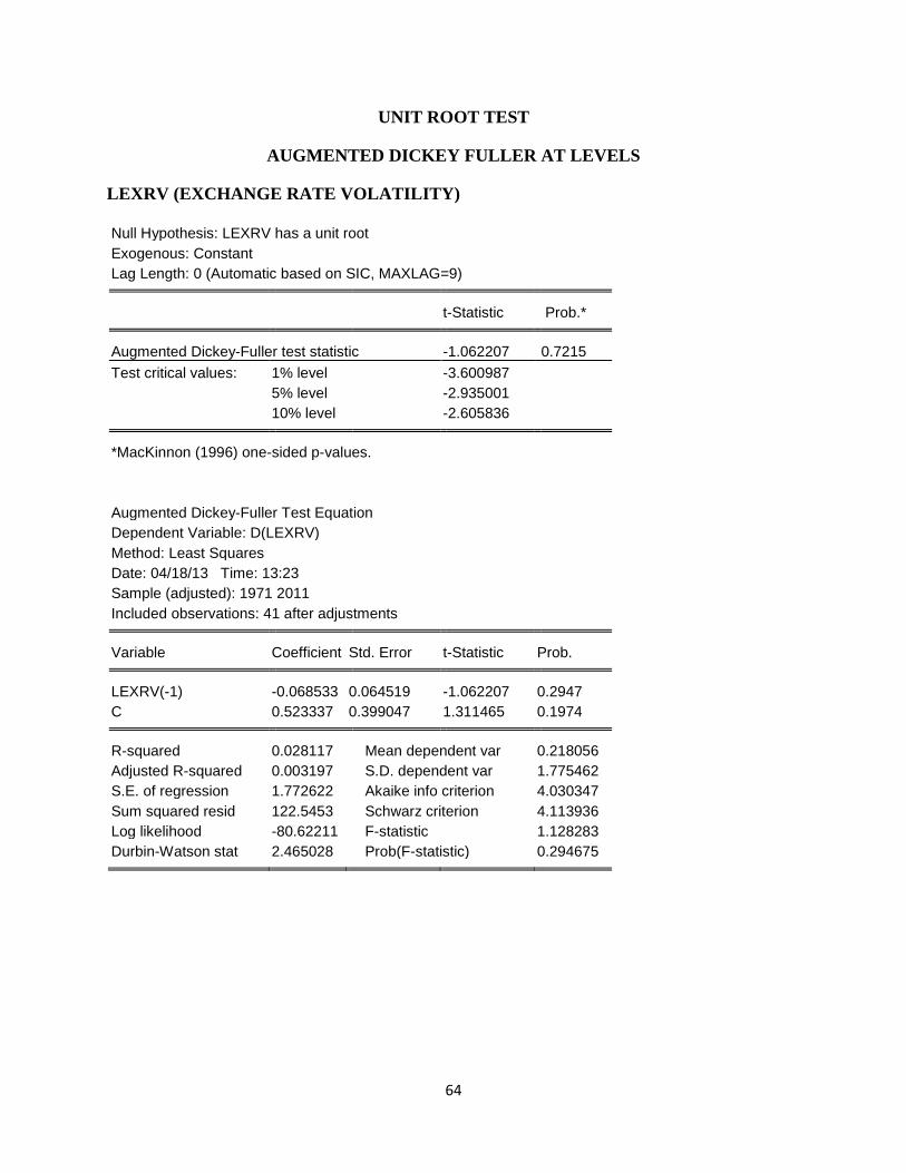
64

UNIT ROOT TEST

AUGMENTED DICKEY FULLER AT LEVELS

LEXRV (EXCHANGE RATE VOLATILITY)

Null Hypothesis: LEXRV has a unit root

Exogenous: Constant

Lag Length: 0 (Automatic based on SIC, MAXLAG=9) t-Statistic Prob.* Augmented Dickey-Fuller test statistic -1.062207 0.7215

Test critical values: 1% level -3.600987

5% level -2.935001

10% level -2.605836 *MacKinnon (1996) one-sided p-values.

Augmented Dickey-Fuller Test Equation

Dependent Variable: D(LEXRV)

Method: Least Squares

Date: 04/18/13 Time: 13:23

Sample (adjusted): 1971 2011

Included observations: 41 after adjustments Variable Coefficient Std. Error t-Statistic Prob. LEXRV(-1) -0.068533 0.064519 -1.062207 0.2947

C 0.523337 0.399047 1.311465 0.1974 R-squared 0.028117 Mean dependent var 0.218056

Adjusted R-squared 0.003197 S.D. dependent var 1.775462

S.E. of regression 1.772622 Akaike info criterion 4.030347

Sum squared resid 122.5453 Schwarz criterion 4.113936

Log likelihood -80.62211 F-statistic 1.128283

Durbin-Watson stat 2.465028 Prob(F-statistic) 0.294675

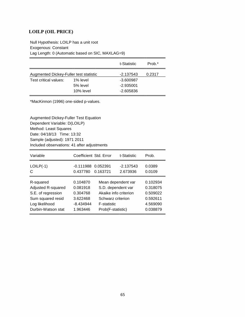
65

LOILP (OIL PRICE)

Null Hypothesis: LOILP has a unit root

Exogenous: Constant

Lag Length: 0 (Automatic based on SIC, MAXLAG=9) t-Statistic Prob.* Augmented Dickey-Fuller test statistic -2.137543 0.2317

Test critical values: 1% level -3.600987

5% level -2.935001

10% level -2.605836 *MacKinnon (1996) one-sided p-values.

Augmented Dickey-Fuller Test Equation

Dependent Variable: D(LOILP)

Method: Least Squares

Date: 04/18/13 Time: 13:32

Sample (adjusted): 1971 2011

Included observations: 41 after adjustments Variable Coefficient Std. Error t-Statistic Prob. LOILP(-1) -0.111988 0.052391 -2.137543 0.0389

C 0.437780 0.163721 2.673936 0.0109 R-squared 0.104870 Mean dependent var 0.102934

Adjusted R-squared 0.081918 S.D. dependent var 0.318075

S.E. of regression 0.304768 Akaike info criterion 0.509022

Sum squared resid 3.622468 Schwarz criterion 0.592611

Log likelihood -8.434944 F-statistic 4.569090

Durbin-Watson stat 1.963446 Prob(F-statistic) 0.038879

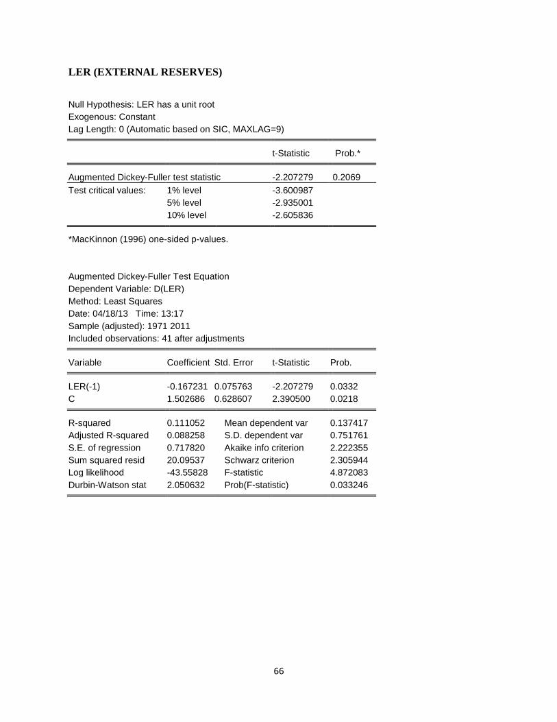
66

LER (EXTERNAL RESERVES) Null Hypothesis: LER has a unit root

Exogenous: Constant

Lag Length: 0 (Automatic based on SIC, MAXLAG=9) t-Statistic Prob.* Augmented Dickey-Fuller test statistic -2.207279 0.2069

Test critical values: 1% level -3.600987

5% level -2.935001

10% level -2.605836 *MacKinnon (1996) one-sided p-values.

Augmented Dickey-Fuller Test Equation

Dependent Variable: D(LER)

Method: Least Squares

Date: 04/18/13 Time: 13:17

Sample (adjusted): 1971 2011

Included observations: 41 after adjustments Variable Coefficient Std. Error t-Statistic Prob. LER(-1) -0.167231 0.075763 -2.207279 0.0332

C 1.502686 0.628607 2.390500 0.0218 R-squared 0.111052 Mean dependent var 0.137417

Adjusted R-squared 0.088258 S.D. dependent var 0.751761

S.E. of regression 0.717820 Akaike info criterion 2.222355

Sum squared resid 20.09537 Schwarz criterion 2.305944

Log likelihood -43.55828 F-statistic 4.872083

Durbin-Watson stat 2.050632 Prob(F-statistic) 0.033246

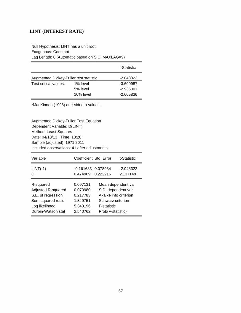
67

LINT (INTEREST RATE)

Null Hypothesis: LINT has a unit root

Exogenous: Constant

Lag Length: 0 (Automatic based on SIC, MAXLAG=9) t-Statistic Prob.* Augmented Dickey-Fuller test statistic -2.048322 0.2660

Test critical values: 1% level -3.600987

5% level -2.935001

10% level -2.605836 *MacKinnon (1996) one-sided p-values.

Augmented Dickey-Fuller Test Equation

Dependent Variable: D(LINT)

Method: Least Squares

Date: 04/18/13 Time: 13:28

Sample (adjusted): 1971 2011

Included observations: 41 after adjustments Variable Coefficient Std. Error t-Statistic Prob. LINT(-1) -0.161683 0.078934 -2.048322 0.0473

C 0.474909 0.222216 2.137148 0.0389 R-squared 0.097131 Mean dependent var 0.025102

Adjusted R-squared 0.073980 S.D. dependent var 0.226315

S.E. of regression 0.217783 Akaike info criterion -0.163083

Sum squared resid 1.849751 Schwarz criterion -0.079494

Log likelihood 5.343196 F-statistic 4.195622

Durbin-Watson stat 2.540762 Prob(F-statistic) 0.047302

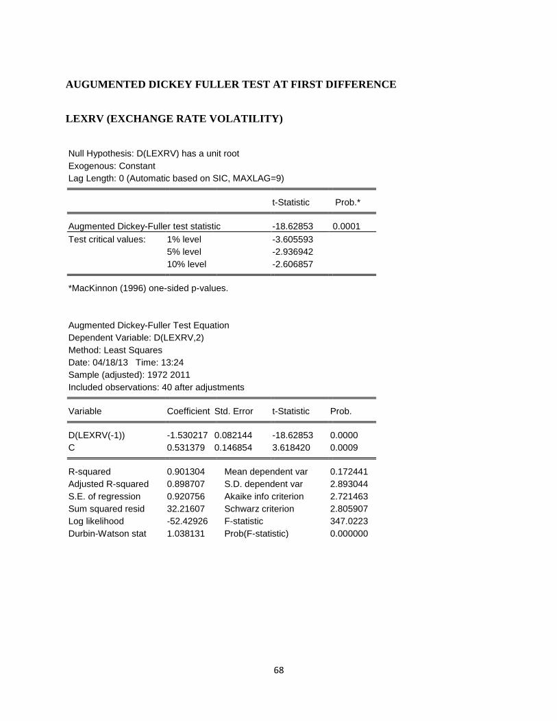
68

AUGUMENTED DICKEY FULLER TEST AT FIRST DIFFERENCE

LEXRV (EXCHANGE RATE VOLATILITY)

Null Hypothesis: D(LEXRV) has a unit root

Exogenous: Constant

Lag Length: 0 (Automatic based on SIC, MAXLAG=9) t-Statistic Prob.* Augmented Dickey-Fuller test statistic -18.62853 0.0001

Test critical values: 1% level -3.605593

5% level -2.936942

10% level -2.606857 *MacKinnon (1996) one-sided p-values.

Augmented Dickey-Fuller Test Equation

Dependent Variable: D(LEXRV,2)

Method: Least Squares

Date: 04/18/13 Time: 13:24

Sample (adjusted): 1972 2011

Included observations: 40 after adjustments Variable Coefficient Std. Error t-Statistic Prob. D(LEXRV(-1)) -1.530217 0.082144 -18.62853 0.0000

C 0.531379 0.146854 3.618420 0.0009 R-squared 0.901304 Mean dependent var 0.172441

Adjusted R-squared 0.898707 S.D. dependent var 2.893044

S.E. of regression 0.920756 Akaike info criterion 2.721463

Sum squared resid 32.21607 Schwarz criterion 2.805907

Log likelihood -52.42926 F-statistic 347.0223

Durbin-Watson stat 1.038131 Prob(F-statistic) 0.000000

69

LOILP (OIL PRICE)

Null Hypothesis: D(LOILP) has a unit root

Exogenous: Constant

Lag Length: 0 (Automatic based on SIC, MAXLAG=9) t-Statistic Prob.* Augmented Dickey-Fuller test statistic -6.058508 0.0000

Test critical values: 1% level -3.605593

5% level -2.936942

10% level -2.606857 *MacKinnon (1996) one-sided p-values.

Augmented Dickey-Fuller Test Equation

Dependent Variable: D(LOILP,2)

Method: Least Squares

Date: 04/18/13 Time: 13:33

Sample (adjusted): 1972 2011

Included observations: 40 after adjustments Variable Coefficient Std. Error t-Statistic Prob. D(LOILP(-1)) -0.988643 0.163183 -6.058508 0.0000

C 0.099525 0.053918 1.845852 0.0727 R-squared 0.491336 Mean dependent var 0.003571

Adjusted R-squared 0.477950 S.D. dependent var 0.451144

S.E. of regression 0.325965 Akaike info criterion 0.644653

Sum squared resid 4.037620 Schwarz criterion 0.729097

Log likelihood -10.89306 F-statistic 36.70552

Durbin-Watson stat 1.986547 Prob(F-statistic) 0.000000

70

LER (EXTERNAL RESERVES)

Null Hypothesis: D(LER) has a unit root

Exogenous: Constant

Lag Length: 0 (Automatic based on SIC, MAXLAG=9) t-Statistic Prob.* Augmented Dickey-Fuller test statistic -6.719037 0.0000

Test critical values: 1% level -3.605593

5% level -2.936942

10% level -2.606857 *MacKinnon (1996) one-sided p-values.

Augmented Dickey-Fuller Test Equation

Dependent Variable: D(LER,2)

Method: Least Squares

Date: 04/18/13 Time: 13:19

Sample (adjusted): 1972 2011

Included observations: 40 after adjustments Variable Coefficient Std. Error t-Statistic Prob. D(LER(-1)) -1.083867 0.161313 -6.719037 0.0000

C 0.139327 0.123278 1.130182 0.2655 R-squared 0.542970 Mean dependent var -0.017044

Adjusted R-squared 0.530943 S.D. dependent var 1.117954

S.E. of regression 0.765662 Akaike info criterion 2.352555

Sum squared resid 22.27706 Schwarz criterion 2.436999

Log likelihood -45.05110 F-statistic 45.14546

Durbin-Watson stat 2.005726 Prob(F-statistic) 0.000000

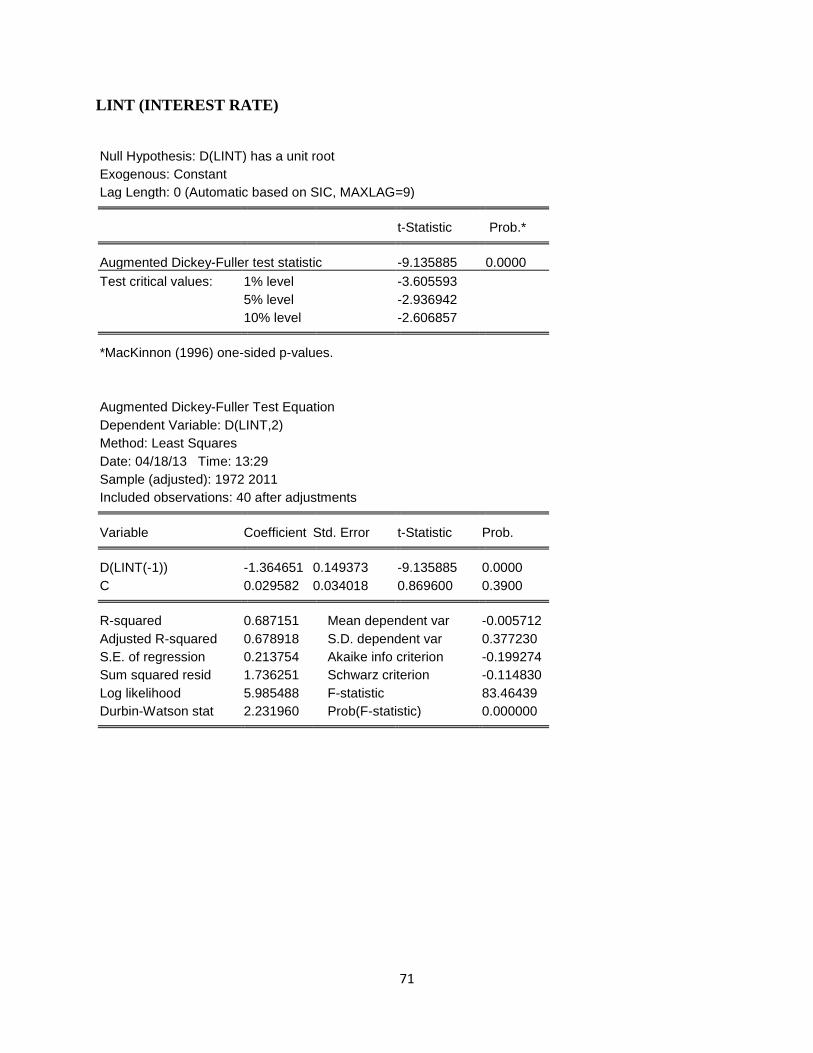
71

LINT (INTEREST RATE)

Null Hypothesis: D(LINT) has a unit root

Exogenous: Constant

Lag Length: 0 (Automatic based on SIC, MAXLAG=9) t-Statistic Prob.* Augmented Dickey-Fuller test statistic -9.135885 0.0000

Test critical values: 1% level -3.605593

5% level -2.936942

10% level -2.606857 *MacKinnon (1996) one-sided p-values.

Augmented Dickey-Fuller Test Equation

Dependent Variable: D(LINT,2)

Method: Least Squares

Date: 04/18/13 Time: 13:29

Sample (adjusted): 1972 2011

Included observations: 40 after adjustments Variable Coefficient Std. Error t-Statistic Prob. D(LINT(-1)) -1.364651 0.149373 -9.135885 0.0000

C 0.029582 0.034018 0.869600 0.3900 R-squared 0.687151 Mean dependent var -0.005712

Adjusted R-squared 0.678918 S.D. dependent var 0.377230

S.E. of regression 0.213754 Akaike info criterion -0.199274

Sum squared resid 1.736251 Schwarz criterion -0.114830

Log likelihood 5.985488 F-statistic 83.46439

Durbin-Watson stat 2.231960 Prob(F-statistic) 0.000000

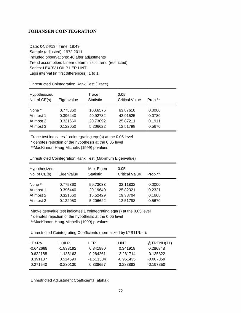
72

JOHANSEN COINTEGRATION

Date: 04/24/13 Time: 18:49

Sample (adjusted): 1972 2011

Included observations: 40 after adjustments

Trend assumption: Linear deterministic trend (restricted)

Series: LEXRV LOILP LER LINT

Lags interval (in first differences): 1 to 1

Unrestricted Cointegration Rank Test (Trace) Hypothesized Trace 0.05

No. of CE(s) Eigenvalue Statistic Critical Value Prob.** None * 0.775360 100.6576 63.87610 0.0000

At most 1 0.396440 40.92732 42.91525 0.0780

At most 2 0.321660 20.73092 25.87211 0.1911

At most 3 0.122050 5.206622 12.51798 0.5670 Trace test indicates 1 cointegrating eqn(s) at the 0.05 level

* denotes rejection of the hypothesis at the 0.05 level

**MacKinnon-Haug-Michelis (1999) p-values

Unrestricted Cointegration Rank Test (Maximum Eigenvalue) Hypothesized Max-Eigen 0.05

No. of CE(s) Eigenvalue Statistic Critical Value Prob.** None * 0.775360 59.73033 32.11832 0.0000

At most 1 0.396440 20.19640 25.82321 0.2321

At most 2 0.321660 15.52429 19.38704 0.1668

At most 3 0.122050 5.206622 12.51798 0.5670 Max-eigenvalue test indicates 1 cointegrating eqn(s) at the 0.05 level

* denotes rejection of the hypothesis at the 0.05 level

**MacKinnon-Haug-Michelis (1999) p-values

Unrestricted Cointegrating Coefficients (normalized by b'*S11*b=I): LEXRV LOILP LER LINT @TREND(71)

-0.642668 -1.838192 0.341880 0.341918 0.286848

0.622188 -1.135163 0.284261 -3.261714 -0.135822

0.391137 0.514593 -1.511504 -0.961435 -0.007859

0.271540 -0.230130 0.338657 3.283883 -0.197350

Unrestricted Adjustment Coefficients (alpha):

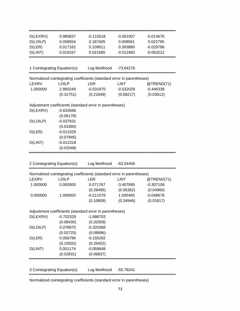
73

D(LEXRV) 0.985837 -0.110518 -0.001007 -0.014676

D(LOILP) 0.058554 0.187405 0.008561 0.022795

D(LER) 0.017162 0.109011 0.393889 -0.029786

D(LINT) 0.019167 0.021685 -0.012482 -0.063212

1 Cointegrating Equation(s): Log likelihood -73.64276 Normalized cointegrating coefficients (standard error in parentheses)

LEXRV LOILP LER LINT @TREND(71)

1.000000 2.860249 -0.531970 -0.532029 -0.446339

(0.31751) (0.21849) (0.68217) (0.03612)

Adjustment coefficients (standard error in parentheses)

D(LEXRV) -0.633566

(0.06178)

D(LOILP) -0.037631

(0.03380)

D(LER) -0.011029

(0.07945)

D(LINT) -0.012318

(0.02048)

2 Cointegrating Equation(s): Log likelihood -63.54456 Normalized cointegrating coefficients (standard error in parentheses)

LEXRV LOILP LER LINT @TREND(71)

1.000000 0.000000 0.071767 -3.407895 -0.307108

(0.29495) (0.95362) (0.04960)

0.000000 1.000000 -0.211078 1.005460 -0.048678

(0.10809) (0.34946) (0.01817)

Adjustment coefficients (standard error in parentheses)

D(LEXRV) -0.702329 -1.686703

(0.08430) (0.20359)

D(LOILP) 0.078970 -0.320368

(0.03725) (0.08996)

D(LER) 0.056796 -0.155292

(0.10932) (0.26402)

D(LINT) 0.001174 -0.059848

(0.02831) (0.06837)

3 Cointegrating Equation(s): Log likelihood -55.78241 Normalized cointegrating coefficients (standard error in parentheses)

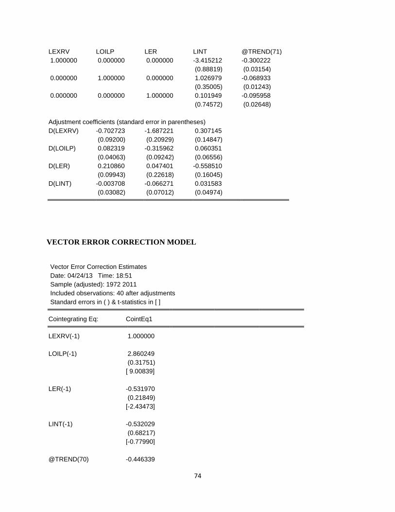
74

LEXRV LOILP LER LINT @TREND(71)

1.000000 0.000000 0.000000 -3.415212 -0.300222

(0.88819) (0.03154)

0.000000 1.000000 0.000000 1.026979 -0.068933

(0.35005) (0.01243)

0.000000 0.000000 1.000000 0.101949 -0.095958

(0.74572) (0.02648)

Adjustment coefficients (standard error in parentheses)

D(LEXRV) -0.702723 -1.687221 0.307145

(0.09200) (0.20929) (0.14847)

D(LOILP) 0.082319 -0.315962 0.060351

(0.04063) (0.09242) (0.06556)

D(LER) 0.210860 0.047401 -0.558510

(0.09943) (0.22618) (0.16045)

D(LINT) -0.003708 -0.066271 0.031583

(0.03082) (0.07012) (0.04974)

VECTOR ERROR CORRECTION MODEL

Vector Error Correction Estimates

Date: 04/24/13 Time: 18:51

Sample (adjusted): 1972 2011

Included observations: 40 after adjustments

Standard errors in ( ) & t-statistics in [ ] Cointegrating Eq: CointEq1 LEXRV(-1) 1.000000

LOILP(-1) 2.860249

(0.31751)

[ 9.00839]

LER(-1) -0.531970

(0.21849)

[-2.43473]

LINT(-1) -0.532029

(0.68217)

[-0.77990]

@TREND(70) -0.446339

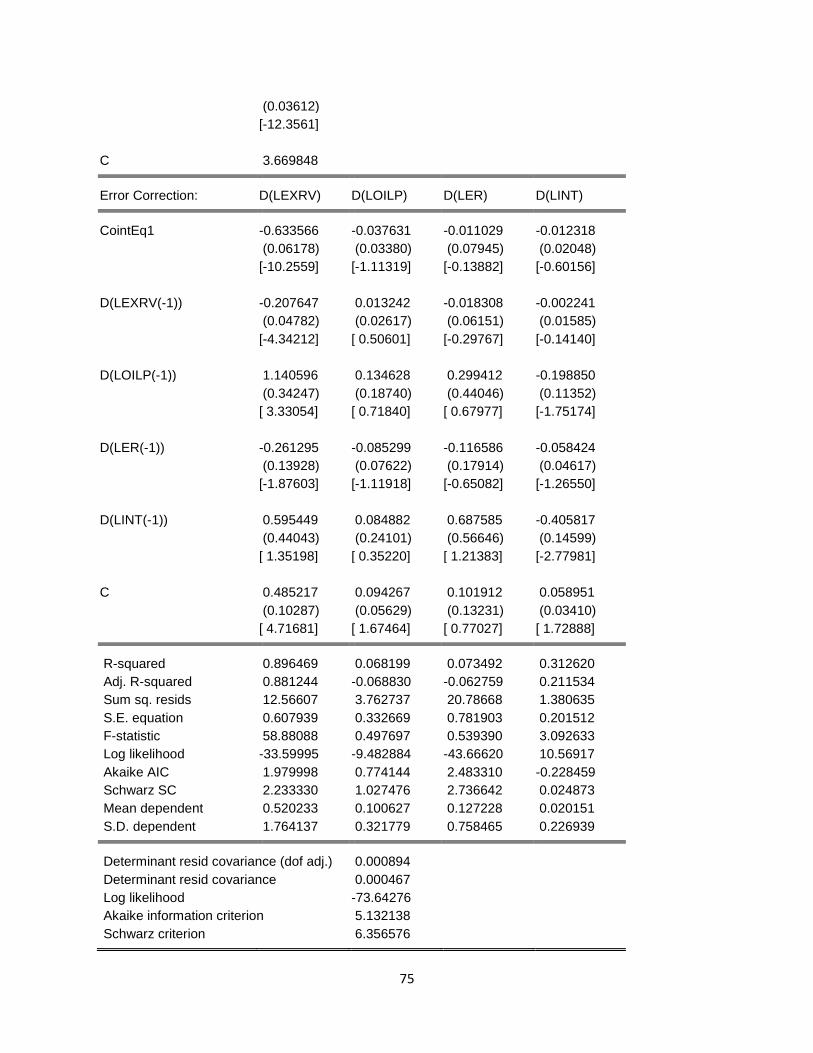
75

(0.03612)

[-12.3561]

C 3.669848 Error Correction: D(LEXRV) D(LOILP) D(LER) D(LINT) CointEq1 -0.633566 -0.037631 -0.011029 -0.012318

(0.06178) (0.03380) (0.07945) (0.02048)

[-10.2559] [-1.11319] [-0.13882] [-0.60156]

D(LEXRV(-1)) -0.207647 0.013242 -0.018308 -0.002241

(0.04782) (0.02617) (0.06151) (0.01585)

[-4.34212] [ 0.50601] [-0.29767] [-0.14140]

D(LOILP(-1)) 1.140596 0.134628 0.299412 -0.198850

(0.34247) (0.18740) (0.44046) (0.11352)

[ 3.33054] [ 0.71840] [ 0.67977] [-1.75174]

D(LER(-1)) -0.261295 -0.085299 -0.116586 -0.058424

(0.13928) (0.07622) (0.17914) (0.04617)

[-1.87603] [-1.11918] [-0.65082] [-1.26550]

D(LINT(-1)) 0.595449 0.084882 0.687585 -0.405817

(0.44043) (0.24101) (0.56646) (0.14599)

[ 1.35198] [ 0.35220] [ 1.21383] [-2.77981]

C 0.485217 0.094267 0.101912 0.058951

(0.10287) (0.05629) (0.13231) (0.03410)

[ 4.71681] [ 1.67464] [ 0.77027] [ 1.72888] R-squared 0.896469 0.068199 0.073492 0.312620

Adj. R-squared 0.881244 -0.068830 -0.062759 0.211534

Sum sq. resids 12.56607 3.762737 20.78668 1.380635

S.E. equation 0.607939 0.332669 0.781903 0.201512

F-statistic 58.88088 0.497697 0.539390 3.092633

Log likelihood -33.59995 -9.482884 -43.66620 10.56917

Akaike AIC 1.979998 0.774144 2.483310 -0.228459

Schwarz SC 2.233330 1.027476 2.736642 0.024873

Mean dependent 0.520233 0.100627 0.127228 0.020151

S.D. dependent 1.764137 0.321779 0.758465 0.226939 Determinant resid covariance (dof adj.) 0.000894

Determinant resid covariance 0.000467

Log likelihood -73.64276

Akaike information criterion 5.132138

Schwarz criterion 6.356576

76