Working Paper 1914 Research Department https://doi.org/10.24149/wp1914

Working papers from the Federal Reserve Bank of Dallas are preliminary drafts circulated for professional comment. The views in this paper are those of the authors and do not necessarily reflect the views of the Federal Reserve Bank of Dallas or the Federal Reserve System. Any errors or omissions are the responsibility of the authors.

Oil Prices, Exchange Rates and Interest Rates

Lutz Kilian and Xiaoqing Zhou

Oil Prices, Exchange Rates and Interest Rates*

Lutz Kilian† and Xiaoqing Zhou‡

April 9, 2018 This version: November 8, 2019

Abstract There has been much interest in the relationship between the price of crude oil, the value of the U.S. dollar, and the U.S. interest rate since the 1980s. For example, the sustained surge in the real price of oil in the 2000s is often attributed to the declining real value of the U.S. dollar as well as low U.S. real interest rates, along with a surge in global real economic activity. Quantifying these effects one at a time is difficult not only because of the close relationship between the interest rate and the exchange rate, but also because demand and supply shocks in the oil market in turn may affect the real value of the dollar and real interest rates. We propose a novel identification strategy for disentangling the causal effects of traditional oil demand and oil supply shocks from the effects of exogenous variation in the U.S. real interest rate and in the real value of the U.S. dollar. We empirically evaluate popular views about the role of exogenous real exchange rate shocks in driving the real price of oil, and we examine the extent to which shocks in the global oil market drive the U.S. real exchange rate and U.S. real interest rates. Our evidence for the first time provides direct empirical support for theoretical models of the link between these variables. JEL codes: E43, F31, F41, Q43 Keywords: Exchange rate; interest rate; oil price; global real activity; commodity; carry trade.

*The views in this paper are solely the responsibility of the authors and should not be interpreted as reflecting the views of the Federal Reserve Bank of Dallas or the Federal Reserve System. We thank Domenico Giannone, Laurent Ferrara, Jeffrey Frankel, Luca Guerrieri, Martin Stürmer, and Rob Vigfusson for helpful comments. †Lutz Kilian, Federal Reserve Bank of Dallas, Research Department, 2200 N. Pearl St., Dallas, TX 75201, USA, lkilian2019@gmail.com. ‡Xiaoqing Zhou, Federal Reserve Bank of Dallas, Research Department, 2200 N. Pearl St., Dallas, TX 75201, USA, xqzhou3@gmail.com.

1  

1. Introduction

There has been much interest in the relationship between the real price of oil, the real value of

the U.S. dollar, and U.S. real market rate of interest since the 1980s.1 Even today, this

relationship remains poorly understood, however, because of the difficulty of identifying

exogenous variation in these variables. We propose a structural vector autoregressive (VAR)

model of the joint determination of these variables. This model is a generalization of the global

oil market of Kilian and Murphy (2014), which has been used in a number of recent studies.2 Our

identification exploits a combination of sign restrictions, exclusion restrictions, and narrative

restrictions motivated by economic theory and extraneous empirical evidence. The model is rich

enough to provide a comprehensive structural analysis of the interaction of the real price of oil

with the real exchange rate and the U.S. real interest rate.

Our analysis sheds light on a range of issues that have been debated for many years, but

have remained unresolved. For example, it has long been conjectured that the real price of oil,

through its effects on the terms of trade, could be a primary determinant of the real value of the

dollar (e.g., Amano and Van Norden 1998; Backus and Crucini 2000; Mundell 2002). Backus

and Crucini (2000), for example, emphasize that “the question … is whether the … change in the

variability of real exchange rates … is related to the similar change in the behavior of oil prices,”

while Mundell (2002) notes that “the question needs to be asked whether the cycle of the dollar

against major currencies is related to the cycle of the dollar commodity prices”.3

 1 Early examples are Krugman (1983a,b), Golub (1983), Frankel (1984), Brown and Phillips (1986), and Trehan (1986). Recent examples include Fratzscher, Schneider and Van Robays (2014), Bützer, Habib and Stracca (2016), and Beckmann, Czudaj and Vipin (2018). 2 Examples include Fattouh, Kilian and Mahadeva (2013), Kilian and Lee (2014), Kilian (2017), Herrera and Rangaraju (2019), Zhou (2019), and Cross, Nguyen and Tran (2019). 3 Implicitly or explicitly the argument articulated in these studies is based on the premise that major changes in the real price of oil reflect exogenous supply disruptions in OPEC countries such that the correlation between changes in the real price of oil and changes in the U.S. real exchange rate can be given a causal interpretation. This traditional view of the determination of the real price of oil has been refuted by more recent studies (see Kilian 2008).

2  

At the same time, other researchers have postulated the exact opposite direction of

causation. For example, Brown and Phillips (1986) and Trehan (1986) conjectured that

exogenous variation in the real exchange rate is responsible for major fluctuations in the real

price of oil. In particular, they suggested that the appreciation of the dollar in the early 1980s

lowered the demand for oil outside of the United States and stimulated the supply of oil outside

of the United States, contributing to the fall in the real price of oil. Similarly, the sustained surge

in the real price of oil in the 2000 has been attributed in part to the declining real value of the

dollar.4

This argument in turn has to be reconciled with the long-standing view that exogenous

fluctuations in the U.S. real rate of interest affect the real price of oil in part through its effect on

the real value of the dollar (e.g., Frankel 1984; Barsky and Kilian 2002; Frankel 2008; Frankel

and Rose 2010). Thus, both the real appreciation of the dollar and the decline in the real price of

oil in the early 1980s may alternatively be explained by an exogenous increase in U.S. real

interest rates under Paul Volcker. The latter argument, however, is called into question by

evidence that the U.S. real interest rate responds to the oil demand and oil supply shocks

responsible for fluctuations in the real price of oil (e.g., Kilian and Lewis 2011; Bodenstein,

Guerrieri and Kilian 2012). Thus, we cannot treat changes in the U.S. real interest rate as

exogenous with respect to the real exchange rate and the real price of oil.

This review illustrates that the real price of oil, the U.S. real exchange rate, and the U.S.

real market rate of interest are determined simultaneously. Understanding cause and effect in the

relationship between these variables therefore requires a structural model. In this paper, we

 4 This view is also consistent with the widely cited rule of thumb in the financial press that the price of oil rises, as the value of the dollar falls. For example, recently, the Wall Street Journal suggested that “oil prices … got a lift from a … slide in the dollar against other currencies” (“U.S. Oil Markets Rise as Saudis Dismiss Supply Concerns”, Wall Street Journal, July 19, 2018, by S. Said and D. Molinsky).

3  

employ a novel identification strategy for disentangling the causal effects of traditional oil

demand and oil supply shocks from the effects of exogenous variation in the real value of the

dollar and in the U.S. real market rate of interest. Our analysis establishes four new facts.

First, we show that 58% of the variation in the U.S. real exchange rate is driven by

shocks that are exogenous with respect to the global oil market, contrary to the results and

conjectures in Amano and van Norden (1998), Backus and Crucini (2000), and Mundell (2002).

Oil supply shocks alone explain only 8% of the unconditional variability in the U.S. real

exchange rate. Flow demand and storage demand shocks account for an additional 31%,

suggesting a modestly important role of actual and expected global business cycle dynamics for

the determination of the real exchange rate.

Second, we provide evidence that exogenous real exchange rate shocks represent demand

shocks in the global market for crude oil. We find robust evidence of a systematic effect of these

shocks on the real price of oil. While this effect is gradual and does not matter much for

explaining sudden changes in the real price of oil, we show that sustained exogenous real

exchange rate appreciations and depreciations may have large cumulative effects over the course

of several years. For example, we show that an exogenous real appreciation of the dollar in the

early 1980s cumulatively lowered the real price of oil over time by 17%, providing empirical

support for the conjectures of Brown and Phillips (1986) and Trehan (1986), even after

controlling for exogenous variation in the U.S. real interest rate. Even larger cumulative effects

are observed during the real depreciation of the dollar between late 2002 and early 2008 and

during its real appreciation between 2011 and 2016.

Third, our framework allows us to examine the impact of exogenous shocks to the U.S.

real interest rate on the real price of oil. Although there is a large literature on how to model the

4  

relationship between interest rates and commodity prices, the problem of estimating the effects

of exogenous changes in the U.S. real interest on the real price of oil has proved elusive to date,

because fluctuations in global real activity and in the real exchange rate tend to confound these

effects in the data. Our structural VAR analysis provides the first direct empirical evidence for a

causal link from U.S. real interest rates to real commodity prices, as described by Frankel (1984,

2008, 2014), among others, while accounting for the endogeneity of all model variables. The

structural VAR framework allows us to empirically evaluate the predictions of Frankel’s

commodity market model and to quantify the effects in question.

Our estimates provide support for some implications of Frankel’s model, while showing

others to be quantitatively unimportant or not robust to generalizations of this model. Most

importantly, we show that an exogenous increase in the U.S. real interest rate causes a modest

and short-lived decline in the real price of oil. Notwithstanding the higher opportunity cost of

holding inventories, emphasized by Frankel, on balance, oil inventories actually increase,

reflecting the decline in global real activity associated with higher U.S. real interest rates. There

is no appreciable response in global oil production, suggesting that the greater incentive for

extracting crude oil emphasized by Frankel is largely offset by the higher capital cost of

investing in future oil production. We also document that exogenous changes to the U.S. real

interest rate have important effects on the U.S. real exchange rate, whereas U.S. real interest

rates are much less sensitive to exogenous changes in the U.S. real exchange rate. Exogenous

variation in the U.S. real market rate of interest explains 22% of the variance of the U.S. real

exchange rate, consistent with the reasoning of Frankel (2008).

Fourth, our results raise the question of whether existing models of the global oil market

that do not explicitly model real exchange rate dynamics and real interest rate fluctuations

5  

remain adequate for understanding the evolution of the real price of oil. We show that, with few

exceptions, previous accounts of the ups and downs in the real price of oil remain approximately

correct, although in some cases the mechanisms become more complicated. For example, our

analysis sheds new light on how the surge in the real price of oil between 2003 and mid-2008

came about. We find that the real depreciation of the U.S. dollar helped reinforce the surge in

flow demand caused by the economic boom in emerging economies. It is, in fact, the second

most important explanation of this sustained surge in the real price of oil. By itself, it accounts

for a cumulative increase of 39% in the real price of oil compared with a 50% cumulative

increase caused by demand shocks directly associated with the global business cycle. In contrast,

real interest rate shocks explain only a 4% cumulative increase in the real price of oil during this

episode. Our evidence challenges the popular view that the U.S. Federal Reserve was responsible

for rising real oil prices in the 2000s. Nor do we find support for the conjecture that exogenous

variation in the U.S. real interest rate associated with loose monetary policy contributed to the

surge in the real price of oil in 1979/80 (Barsky and Kilian 2002). There is some evidence that

the tightening of monetary policy in the 1980s contributed to the decline in the real price of oil,

but the cumulative effect is only imprecisely estimated.

The remainder of the paper is organized as follows. In section 2, we discuss the structural

econometric model with particular attention to the economic rationale of the identifying

restrictions. In section 3, we study the transmission of the structural shocks to the model

variables. Section 4 examines the key determinants of the variability of the data. In section 5, we

estimate the cumulative effect of sustained exogenous real appreciations and depreciation on the

real price of oil. Section 6 re-examines the historical narrative of the major oil price fluctuations

since the late 1970s through the lens of the structural model. The conclusion is in section 7.

6  

2. Identification and Estimation

The starting point of our analysis is the structural vector autoregressive global oil market model

of Kilian and Murphy (2014), which has become the workhorse model for assessing the relative

importance of oil demand and oil supply shocks for the evolution of the real price of oil. Unlike

earlier global oil market models such as Kilian (2009) or Kilian and Murphy (2012) this model

explicitly incorporates shocks to the storage demand for oil reflecting shifts in oil price

expectations.5

The baseline oil market model includes the percent change in the global production of

crude oil ( tq ), as reported by the U.S. Energy Information Administration; a measure of

cyclical variation in global real economic activity ( rea t ) originally proposed by Kilian (2009) 6;

the log real price of oil ( pt ) obtained by deflating the U.S. refiners’ acquisition cost for imported

crude oil by the U.S. CPI for all urban consumers; and a proxy for the change in global crude oil

inventories ( invt ), as discussed in Kilian and Murphy (2014) and Kilian and Lee (2104). We

extend this model by including the log of the U.S. trade-weighted real exchange rate ( rxrt ), as

reported by the Federal Reserve Board (Loretan 2005), and the U.S. real market rate of interest

( ). Following Frankel (2008), we use the nominal U.S. one year treasury rate, adjusted for

inflation over the preceding years as a proxy for expected inflation.7 Throughout the paper, trade-

 5 For a review of merits of this approach and a comparison with alternative approaches to modeling the global oil market see Herrera and Rangaraju (2019) and Kilian (2019a). 6 The Kilian index of global real economic activity is based on data for bulk dry cargo ocean shipping freight rates. It is arguably the most widely used indicator of global real economic activity in the oil market literature. As discussed in Kilian and Zhou (2018), this index has several conceptual advantages compared with proxies for global industrial production when it comes to modeling the global market for crude oil. We use the version of the index discussed in Kilian (2019b) from https://sites.google.com/site/lkilian2019/research/data-sets. 7 This interest rate is intended to reflect the cost of borrowing in financial markets. We are not modeling monetary policy or the link from policy rates to market interest rates. Our specification allows us to circumvent the fact that this link is not stable during the period of quantitative easing.

rt

7  

weighted U.S. real exchange rate is defined in foreign consumption units relative to U.S.

consumption units, with an increase in the real exchange rate representing a real appreciation of

the dollar. For simplicity, we will refer to this series as the U.S. real exchange rate. All data are

monthly and have been seasonally adjusted. The sample extends from 1973.2 to 2018.6.

Let ( , rea , p , inv ,r ,rxr )t t t t t t ty q be generated by the covariance stationary structural

VAR(24) process

0 1 1 24 24.... ,t t t tB y B y B y w

where the stochastic error tw is mutually uncorrelated white noise and the deterministic terms

have been suppressed for expository purposes. Setting the lag order to 24 allows the model to

capture long cycles in the real price of oil. The reduced-form errors may be written as

where 10B denotes the structural impact multiplier matrix,

1 1 24 24... ,t t t tu y A y A y  and 10 ,l lA B B 1,...,24.l The { }ij th element of 1

0 ,B denoted 0ijb ,

represents the impact response of variable i to structural shock ,j where 1,...,6i and

1,...,6 .j Given the reduced-form estimates, knowledge of 10B suffices to recover estimates

of the structural impulse responses, variance decompositions and historical decompositions from

the reduced-form estimates, as discussed in Kilian and Lütkepohl (2017).

Let flow supply flow demand storage demand other oil demand r rxr, , , , , ,t t t t t t tw w w w w w w where flow supplytw denotes

a shock to the flow supply of oil, flow demandtw denotes a shock to the flow demand for oil,

storage demandtw denotes a shock to storage demand (or, equivalently, speculative demand), and

other oil demandtw is a conglomerate denoting all other shocks to the demand for oil such as shocks to

preferences for oil, shocks to the oil inventory technology, or politically motivated changes in the

10 ,t tu B w

8  

Strategic Petroleum Reserve. As in the related literature, our analysis focuses on the first three

oil market shocks that have an explicit structural interpretation. rtw denotes an exogenous shock

to the U.S. real market rate of interest, defined as an unexpected change in the U.S. real interest

rate not explained by any of the oil market shocks. Finally, rxrtw denotes an exogenous shock to

the U.S. real exchange rate, defined as an unexpected change in the real exchange rate not caused

by the exogenous variation in the U.S. real interest rate or by oil demand and oil supply shocks.

All shocks but the real interest rate shock are normalized to represent a shock that raises the real

price of oil.

It is useful to elaborate on the nature of the real exchange rate shock. In standard open

economy models with non-state contingent bonds, the exchange rate is governed by the

uncovered interest parity (UIP) condition. This no-arbitrage condition pins down the nominal

exchange rate. As long as UIP holds, there is no room for exogenous exchange rate shocks in

these models. We can, however, interpret the exchange rate shock in the baseline VAR model as

being driven by unmodeled shifts in global interest rate differentials that are not implicitly

explained by the other structural shocks in the model. Moreover, even in the absence of shocks

entering the UIP condition directly, many shocks can influence the nominal exchange rate. For

example, with home bias in consumption, an exogenous consumption preference shock abroad

would be indistinguishable from a shock that temporarily suspends the no-arbitrage condition

underlying the UIP relationship, since we do not explicitly model consumption abroad. To the

extent that such a shock is not captured by the demand shocks in the baseline VAR model, it

would result in exogenous variation in the real exchange rate in the VAR model. In this sense,

the real exchange rate shock may be viewed as a measure of exogenous variation in the

unmodeled determinants of the real exchange rate. Our approach is consistent with a large

9  

literature on the difficulty of explaining exchange rate fluctuations based on economic

fundamentals.

2.1. Identifying Restrictions

The model consists of two blocks. One block includes the first four variables and describes the

global oil market. The model imposes sign restrictions on the elements of the oil market block.

These inequality restrictions render the model set-identified. The other block consists of the real

U.S. market rate of interest and the U.S. real exchange rate. The model is block recursive in that

it imposes that there is no contemporaneous feedback from the second block to the oil market

variables. The variables in the second block are allowed to respond contemporaneously to all

structural shocks in the first block. The sign and exclusion restrictions on the elements of 10B are

summarized in expression (1):

0 flowsupply14

rea 0 flow demand24

p 0 storagedemand340 otheroildem44

r 0 0 0 0 051 52 53 54 55

rxr 0 0 0 0 0 061 62 63 64 65 66

0 0

0 0

0 0

0 0

0

qt t

t t

t tinv

t t

t

t

u b w

u b w

u b w

u b w

u b b b b b

u b b b b b b

and

exogenous rt

exogenous rxrt

w

w

(1)

2.1.1. Identifying restrictions in the oil market block

It is useful to first consider the oil market block in isolation. The identification of the shocks in

the oil market block is achieved by a combination of static sign restrictions, bounds on the one-

month price elasticities of oil demand and oil supply that may be expressed as inequality

restrictions on functions of selected impact responses, dynamic sign restrictions on selected

structural impulse response functions, and narrative sign restrictions on the historical

decomposition of the real price of oil.

10  

Sign restrictions in the oil market block

The static sign restrictions in the oil market block are conventional. An unexpected disruption of

the flow supply of crude oil is represented as an unexpected reduction in global oil production

that raises the real price of oil and lowers global real activity and crude oil inventories. As in

related studies, the sign restriction on the response of global real activity to a negative flow

supply shock is imposed not only on impact, but for the first 12 months. This additional dynamic

sign restriction ensures that this response corresponds to conventional views of the effects of oil

supply shocks. An exogenous increase in flow demand raises global real activity, global oil

production and the real price of oil, but lowers oil inventories. An exogenous increase in storage

demand raises oil inventories, the real price of oil, and global oil production, while lowering

global real activity. We also follow the recent literature in imposing the restriction that the

response of the real price of oil to the first three shocks is positive not only on impact, but for the

first 12 months (e.g., Inoue and Kilian 2013; Kilian 2017). The residual oil demand shock is

implicitly defined as the complement to the other shocks.

Bounds on the impact price elasticities of oil demand and supply

The sign restrictions on the impact responses are strengthened by imposing bounds on the impact

price elasticities of demand and supply. Since these elasticities can be expressed as functions of

the impact responses to exogenous supply and demand shocks, respectively, elasticity bounds

can be written as inequality restrictions on nonlinear functions of the elements of 10B (Kilian and

Murphy 2012, 2014, Kilian 2019a).

In defining the price elasticity of oil demand, we avoid the common mistake of imposing

the restriction that the production of crude oil equals the consumption of crude oil at each point

in time. We instead incorporate the response of oil inventories in measuring changes in the use of

11  

oil in response to exogenous flow supply shocks, as discussed in Kilian and Murphy (2014). We

impose that the implied impact price elasticity of demand cannot exceed the long-run price

elasticity of oil demand, which is set to -0.8 based on extraneous microeconomic estimates in

Hausman and Newey (1995) and Yatchew and No (2001).

We follow Zhou (2019) in imposing a bound of 0.04 on the impact price elasticity of oil

supply. There are two motivations for imposing a bound close to zero. First, economic theory

implies that the optimal response of oil producers to an oil price change induced by oil demand

shifts is to adjust investment in future oil production rather than the level of oil production from

existing wells (Anderson, Kellogg, and Salant 2018).8 Second, although there are no

microeconomic estimates of the global one-month price elasticity of oil supply, recent

microeconomic estimates based on regional data are close to zero, consistent with economic

theory. For example, Newell and Prest (2019) estimate the U.S. price elasticity of oil supply for

conventional crude to be 0.017 (with a standard error of 0.006) based on a comprehensive data

set for U.S. oil producers from Texas, North Dakota, California, Oklahoma and Colorado.

Our upper bound of 0.04 on the aggregate global oil supply elasticity is about four

standard errors larger than this microeconomic estimate. Newell and Prest’s corresponding

supply elasticity estimate for shale oil is effectively zero, which makes economic sense given

that it takes 4-12 weeks to complete shale oil wells (see Kilian 2019a). Similar results hold for

oil producers outside the United States. Kilian (2019a) estimates Saudi Arabia’s one-month price

elasticity of oil supply to be 0.014. The latter study also discusses why higher oil supply

elasticity estimates that have been reported in the recent literature are econometrically invalid

 8 A similar point was made by Kilian (2009) who attributed the sluggishness of the supply response to the “costs of adjusting oil production and the uncertainty about the state of the crude oil market” (p. 1059).

12  

and economically implausible.9

Narrative sign restrictions on the historical decomposition of the real price of oil

These identifying restrictions are complemented by additional narrative sign restrictions.

Narrative sign restrictions refer to restrictions in the signs or relative magnitudes of structural

shocks or historical decompositions. They were first employed by Kilian and Murphy (2014) for

selecting the most economically plausible model among the set of admissible structural models

in that study. This idea was subsequently generalized and formalized by Antolin-Diaz and

Rubio-Ramirez (2018).

Our narrative sign restrictions relate to events in 1990, when Iraq invaded Kuwait. It is

uncontroversial that the resulting spike in the oil price in 1990 was caused by a combination of

negative flow supply and positive storage demand shocks. We impose the restriction that not

only the flow demand shock made at best a minimal contribution to this oil price increase, but

that both the flow supply shock and the storage demand shock had some impact. In practice, we

impose the narrative sign restriction that the cumulative effect of the flow supply shock from

June 1990 to October 1990 exceeded 0.1 on a log-scale (or approximately 10%) and that of the

storage demand shock from June 1990 to October 1990 also exceeded 0.1, while that of the flow

demand shock is bounded from above by 0.1. In the case of storage demand shocks, we include

the month leading up to this war, given evidence in Kilian and Murphy (2014) that rising

political tensions in the Middle East increased storage demand even before the war broke out.

Our results are robust to reasonable variation in the magnitude of these bounds.

2.1.2. Restrictions on the feedback from real interest rate and real exchange rate shocks to

the variables in the oil market block

 9 Further discussion of the sensitivity of oil market VAR estimates to this bound can be found in Kilian and Murphy (2012), Zhou (2019), and Herrera and Rangaraju (2019).

13  

We now focus on the last two columns of 10 .B The exclusion restrictions in the upper-right block

of 10B are central for disentangling the effects of exogenous real interest rate and real exchange

rate shocks from oil demand and oil supply shocks. The block-recursive structure of 10B

embodies the assumption that the real price of oil is predetermined with respect to the U.S. real

market rate of interest and the U.S. real exchange rate. Put differently, innovations in the real

price of oil may move the real exchange rate contemporaneously, but exogenous shocks to the

real exchange rate will not affect the real price of oil within the same month, but only with a

delay. The restriction that ptu does not depend on rxr

tu implies that 0B is block recursive and

hence 0 0 016 26 36b b b 0

46 0.b

These exclusion restrictions are motivated by independent empirical evidence in Kilian

and Vega (2011) who studied the response of the exchange rate and the price of oil to a wide

range of daily U.S. macroeconomic news. News here is defined as the difference between

announcements about the latest macroeconomic data releases and market expectations about

these announcements immediately before their release. Kilian and Vega assessed the individual

and joint effect on the price of oil of about 30 U.S. macroeconomic news including the nonfarm

payroll, the Fed target rate, the unemployment rate, the consumer price index, and housing starts,

for example. They found no response in the daily price of oil within the 20 business days

following these news shocks, but a strong and statistically significant response in the exchange

rate.10 This evidence suggests that there cannot be indirect feedback from exogenous exchange

 10 Fratzscher et al. (2014) confirmed these results using more recent data. Datta et al. (2019), using a much smaller set of U.S. macroeconomic news than Kilian and Vega (2011) and restricting attention to the response of the price of oil to these news within the same day, show that during the six years when the zero-lower bound was binding, two of twelve news variables had a much larger effect on the price of oil than reported in Kilian and Vega (2011). Unlike Kilian and Vega (2011), however, Datta et al. do not report data-mining robust p-values, making it impossible to judge the statistical significance of their estimates, and the 2R of their regression including all twelve predictors is only 3%, so the extent of the feedback appears negligible even during the zero-lower bound period.

14  

rate variation to the price of oil at the one-month horizon because, if there were, the price of oil

would have shown a strong and statistically significant response to U.S. macroeconomic news

much like the exchange rate.11 Thus, the price of oil is predetermined with respect to the

exchange rate at monthly frequency. Although the evidence in Kilian and Vega (2011) regarding

the exchange rate responses is based on the response of the nominal U.S. dollar-DM exchange

rate, one would expect this result to extend also to the U.S. real exchange rate, given that much

of the variation in the real exchange rate is driven by the nominal exchange rate.

A similar argument can be made regarding the response of the oil market block to

exogenous shocks to the U.S. real market rate of interest. Kilian and Vega (2011) show that the

long-term U.S. interest rate responds to U.S. macroeconomic news within the month, whereas

the price of oil does not, allowing us to the impose the restrictions 0 0 015 25 35b b b 0

45 0.b

The latter set of restrictions is also consistent with evidence in Kilian and Vega that news about

the federal funds rate target do not move the price of oil within the same month.12 Together these

two sets of exclusion restrictions imply the block recursive structure imposed in equation (1).

2.1.3. Other restrictions on the responses to real interest rate and real exchange rate shocks

We now turn to the identifying restrictions on the responses of the variables in the lower-right

block of 10 .B We employ both static and dynamic sign restrictions.

Exclusion restriction on 056b

The assumption 056 0b allows us to distinguish between exogenous variation in the real

 11 Our argument requires us to identify exogenous variation in the exchange rate. The source of this exogenous variation is not important for the argument. When assessing the possibility of contemporaneous feedback. it suffices to have one source of exogenous variation in the exchange rate. We do not require all possible sources of exogenous variation. In particular, the macroeconomic news in question need not be global. U.S. macroeconomic news are sufficient. 12 Similarly, Rosa (2014, p. 302) reported a small and statistically insignificant response of the daily oil futures price to surprise changes in the federal funds target rate at daily frequency. 

15  

exchange rate and in the real interest rate. This restriction means that the real U.S. market rate of

interest responds to exogenous real exchange rate shocks with a delay of at least one month. This

restriction is directly supported by evidence in Clarida, Gali and Gertler (1998) that the U.S. real

exchange rate is not helpful in predicting U.S. inflation and real output and can be excluded from

the U.S. policy reaction function. If an exogenous real dollar appreciation does not affect

expectations of U.S. inflation and real output, there is no reason for the central bank to lower its

policy rate. As a result, the real market rate of interest remains unchanged on impact, justifying

the restriction 056 0.b

The “disconnect” between changes in exchange rates, inflation and domestic real activity

has also been discussed by Mishkin (2008). The extent to which a depreciation of the domestic

current currency causes inflation expectations depends on how much this shock is passed on first

to import prices and from there to overall consumer prices. Mishkin (2008) notes that there are

good microeconomic reasons why even import prices remain comparatively stable, as the

exchange rate fluctuates, including cross-border production, a high share of distribution costs,

local currency pricing, and pricing to market. Based on several case studies, macroeconomic

time series evidence and microeconomic evidence, he concludes that under a stable monetary

regime the pass-through to consumer price inflation empirically tends to be negligible even after

substantial depreciations of the domestic currency. This result holds even for comparatively open

industrialized economies. It is even more relevant for a relatively closed economy such as the

United States. Likewise, Mishkin (2008) notes that the response of domestic real activity can be

shown to be muted under weak and empirically plausible conditions, providing further credence

to our identifying assumption of a zero impact response of the real market rate of interest.

Incorporating the Insights of Frankel’s Model of Real Commodity Prices

16  

As noted in the introduction, it has been common to associate increases in the real price of oil

price not only with declines in the real value of the dollar, but also with exogenous declines in

the U.S. real interest rate (e.g., Frankel and Hardouvelis 1985; Barsky and Kilian 2002; Frankel

2008, 2012, 2014; Frankel and Rose 2010; Akram 2009). For example, Frankel (1984) attributes

the decline in real commodity prices in the early 1980s not to the real appreciation of the dollar,

as stressed by Brown and Phillips (1986) and Trehan (1986), but to high U.S. real interest rates.

As Frankel’s model of commodity prices shows, this relationship may be explained by

three channels. First, low real interest rates discourage oil production. The lower the real interest

rate, the smaller is the incentive for oil producers to extract oil from below the ground because

the proceeds from the sale are earning less interest. Second, low real interest rates may cause

speculation in real assets such as commodities in the form of inventory holdings. Conversely,

high real interest rates raise the opportunity cost of holding oil inventories and lower the demand

for oil storage. For example, in the early 1980s, oil inventories were liquidated, as the expected

demand for oil fell and real interest rates rose, putting downward pressure on the real price of oil.

Third, low real dollar interest rates (relative to the interest rate abroad) may cause the U.S. dollar

to depreciate, which in turn stimulates demand for oil, raises global real activity, and increases

the real price of oil. Thus, real exchange rate fluctuations, rather than being exogenous, may in

turn be caused by real interest rate shocks.

Although the theoretical arguments that exogenous real interest rate shocks affect the real

price of oil are strong, quantifying these effects empirically has been difficult because

fluctuations in global real activity and in the real exchange rate tend to confound the effects of

U.S. real interest rate shocks. Thus, more often than not, empirical research has simply

abstracted from real interest rate dynamics. Our analysis seeks to incorporate these additional

17  

theory-driven restrictions. It should be noted that the implications of Frankel’s model do not

apply to the impact period in our monthly model, because, as we have shown, the real price of oil

(and hence other oil market variables) do not move on impact in response to interest rate shocks.

Rather Frankel’s model generates additional dynamic sign restrictions. For example, Frankel’s

model predicts that the dollar appreciates in real terms in response to an exogenous increase in

the U.S. real interest rate, while global real economic activity declines.

Not all of the dynamic sign restrictions in Frankel’s model are robust to changes in the

model structure, however. For example, Frankel’s model does not include capital. If it did,

higher U.S. real interest rates would raise the capital cost of oil production (and hence would

lower the level of oil production), rendering the sign of the response of oil production

ambiguous. Likewise, higher U.S. real interest rates need not be associated with an accumulation

of oil inventories, because the implied decline in real activity causes an accumulation of oil

inventories. Thus, only the negative responses of global real activity and the positive responses

of the U.S. real exchange rate to an exogenous real interest rate increase beyond the impact

period are robust implications of Frankel’s model. We impose these two additional dynamic sign

restrictions in estimating the structural VAR model.

2.1.4. Discussion

The identification of our model relies on a combination of inequality restrictions and

exclusion restrictions on the impact multiplier matrix. It may seem that one could have

approached this problem alternatively based on sign restrictions only. This is not the case. Not

only does the evidence we discussed rule out the possibility of using sign restrictions to identify

exogenous variation in the U.S. real interest rate and U.S. real exchange rate, but, in fact, the sign

of the impact responses to a real exchange rate shock would be indistinguishable from the signs

18  

implied by a flow demand shock. In other words, the structural model would reduce to a

conventional oil market model that makes no distinction between these two shocks. Likewise, it

can be shown that the signs of the responses to an exogenous increase in the U.S. real market rate

of interest that can be pinned down a priori do not allow one to uniquely identify this shock.

2.2. Estimation and Inference

The model is estimated by state-of-the-art Bayesian methods, building on Arias et al. (2018) and

Antolin-Diaz and Rubio-Ramirez (2018). We postulate a diffuse Gaussian-inverse Wishart prior

for the reduced-form VAR parameters and a uniform prior for the rotation matrix .Q Given the

inequality and exclusion restrictions, the set of admissible structural models is constructed, as

discussed in Kilian and Lütkepohl (2017). Let 1,..., pA A A denote the autoregressive slope

parameters and u the residual variance-covariance matrix. For a given realization of A and of

the lower triangular matrix ( )uP chol with positive diagonal elements, we draw realizations

of the matrix Q from the space of 6 6 orthogonal matrices by generating at random many 4 4

matrices W consisting of 0,1NID draws. For each ,W we apply the QR decomposition

W QR with the diagonal of the upper triangular matrix R normalized to be positive, and let

0.

0 1

QQ

Then a candidate solution for 10B is ,PQ since .KQQ I We use each of these candidate

solutions in conjunction with A to construct the candidate structural models and their structural

impulse responses. This procedure is repeated for a large number of posterior draws for , uA

to account for parameter estimation uncertainty.

The construction of the set of admissible draws from the posterior distribution of the

19  

structural responses involves a reweighting of the candidate solutions. First, the imposition of

zero restrictions on 10B renders invalid the standard algorithm for generating draws from sign-

identified VAR models, as described in Rubio-Ramirez et al. (2010). This problem may be

addressed by implementing the importance sampler discussed in Arias, Rubio-Ramirez and

Waggoner (2018) that reweights the candidate solutions identified based on inequality and zero

restrictions on the impulse responses without imposing narrative sign restrictions.13 Second, the

imposition of narrative sign restrictions requires the use of another importance sampler, as

discussed in Antolin-Diaz and Rubio-Ramirez (2018). The latter importance sampler is applied

to the set of admissible models identified by both restrictions on the impulse responses and

narrative sign restrictions. This additional step is needed because sign restrictions on the

historical decomposition (unlike more conventional sign restrictions on impulse response

functions) restrict the space of the structural errors and hence the likelihood.14

An additional challenge is that sign-identified VAR models generate no point estimates.

Some users report so-called posterior median response functions instead. Several studies have

observed that this practice confounds estimates from different structural models and tends to

distort the dynamics implied by the estimated models (e.g., Fry and Pagan 2011; Kilian and

Murphy 2012; Inoue and Kilian 2013; Kilian and Lütkepohl 2017; Herrera and Rangaraju 2019).

Moreover, the associated pointwise impulse response error bands understate the true uncertainty

about the model estimates. There are readily available econometric solutions to this problem in

sign-identified VAR models, as discussed in Inoue and Kilian (2013), but not for models

including additional exclusion restrictions.

 13 The effective sample size in our application is 73% as a share of the draws satisfying the sign and zero restrictions, which is comparable to the applications discussed in Arias et al. (2018). 14 We employ 40,000 random draws of the set of structural errors to ensure the reliability of the importance weights.

20  

In this paper, we instead report the full set of impulse response functions for all

admissible structural models. This approach is feasible because in models identified by many

inequality, exclusion, and narrative restrictions the degree of uncertainty tends to be smaller than

in agnostic models based on few restrictions. For variance decompositions, we report posterior

means, given that pointwise posterior medians violate the adding-up constraint underlying the

construction of variance decompositions. Finally, for historical decompositions, we report

posterior median estimates for the cumulative contribution of each shock over selected

subperiods. Inference is conducted based on the posterior quantiles for the cumulative

contribution of each shock. This approach avoids confounding estimates from different structural

models.15

3. Understanding the Transmission of Shocks

Before addressing more substantive questions, it is useful to examine the dynamics implied by

the estimated structural model. This evidence helps us understand how structural shocks are

transmitted. In particular, (1) it helps understand the economic channels through which real

exchange rate and real interest rate shocks are propagated to the global oil market, (2) is allows

us to quantify the extent to which the U.S. real market rate of interest and the real exchange rate

respond to the shocks that drive the global oil market, and (3) it sheds light on the relationship

between the U.S. real exchange rate and the U.S. real market rate of interest.

3.1. Responses to U.S. Real Interest Rate Shocks

Figure 1 shows the responses of the model variables to an exogenous increase in the U.S. real

 15 In constructing the posterior distribution, we bound the dominant root of the VAR process at 0.991019. This restriction implies that the effect of a one percent shock at the beginning of the sample on the model data is reduced to at most 1% at the end of a sample. This bound ensures that posterior draws from the historical decomposition closely resemble the actual historical data for the real price of oil. Without this bound, no meaningful analysis of the cumulative effects of the structural shocks on the real price of oil or the real exchange rate is possible. For a similar type of restriction see Antolin-Diaz and Rubio-Ramirez (2018).

21  

market rate of interest. The large, sustained and precisely estimated real appreciation of the

dollar in response to an increase in the U.S. real market rate of interest suggests that exogenous

U.S. real interest rate shocks are a potentially important determinant of variation in the U.S. real

exchange rate. It confirms that it is important to control for real interest rate shocks in assessing

the effect of changes in the real exchange rate on real commodity prices. An exogenous increase

in the U.S. real interest rate also results in a precisely estimated reduction in global real activity.

Although we restricted the sign of these response functions in estimating the structural model,

the response estimates in Figure 1 provide useful information about the magnitude of the effects

in question and about how precisely they can be estimated. Of even greater interest, of course,

are the signs of the model responses that were not restricted a priori, notably the response of the

real price of oil, but also the responses of oil inventories and of oil production.

As predicted by Frankel’s model, the real price of oil declines initially in response to

higher U.S. real interest rates. Thus, there is empirical support for one of the key implications of

Frankel’s model at least at short horizons. However, even the most negative short-run response

of the real price of oil that is consistent with the data is small. It is worth stressing that this

conclusion would be robust to any additional restrictions one may wish to impose (such as

additional dynamic sign restrictions on the response of the real price of oil to interest rate shocks,

for example). Moreover, beyond the first quarter, there is considerable uncertainty about the sign

and magnitude of the interest rate response.

The response of the level of global oil inventories is slightly negative after one month,

but is mostly positive at longer horizons. This evidence means that the change in the opportunity

cost of holding oil inventories emphasized by Frankel is quantitatively less important than the

accumulation of oil inventories associated with a decline in global real activity. Finally, the sign

22  

of the response of the level of global oil production is generally ambiguous, consistent with our

earlier observation that this effect could be positive or negative, once taking account of the

higher capital cost of expanding oil production.

3.2. Responses to an Exogenous Real Depreciation of the U.S. Dollar

Our analysis also provides direct evidence in support of a transmission of real exchange rate

shocks to the real price of oil. Figure 2 shows the responses of the oil market variables to an

exogenous real depreciation of the dollar. The real price of oil increases for at least half a year.

Global real activity also expands. Both responses tend to be hump-shaped. The level of global

oil production rises with some delay, while the level of inventories unambiguously declines.

These patterns are consistent with the interpretation of real exchange rate shocks as shocks to the

demand for oil. A real depreciation makes it less expensive for countries other than the United

States to import oil (and other industrial commodities traded in U.S. dollars), raising global real

activity and the real price of oil.

Although it is conceivable that a real depreciation of the dollar would also affect the

supply of oil by reducing the incentives to convert oil below the ground into dollar assets, as

noted by Brown and Phillips (1986), this interpretation can be ruled out. A real depreciation

would discourage oil producers outside the United States from producing, causing a decline in

oil production, which is inconsistent with the positive response of global oil production in Figure

2. That response, however, is consistent with oil production responding to the increase in the real

price of oil caused by a demand boom. It is also consistent with a decline in oil inventories, as

refiners smooth their production by drawing down oil inventories. We conclude that real

exchange rate shocks are quite similar to flow demand shocks in conventional global oil market

models, except that their impact effect on oil market variables is constrained to be zero.

23  

3.3. Responses of the Real Exchange Rate to Oil Demand and Oil Supply Shocks

Conversely, we may ask what the effect is of oil demand and oil supply shocks on the U.S. real

exchange rate. Interest in the effects of real oil price shocks on the real exchange rate dates back

to the early 1980s. Golub’s (1983) and Krugman’s (1983a,b) work in this regard stands out in

that it focuses on the implications of an exogenous oil price increase for the real value of the

dollar relative to major currencies. These studies concluded that the dollar will depreciate against

major currencies if the income transfer from the United States to foreign oil producers associated

with an increase in the real price of oil lowers the demand for U.S. dollars and raises the demand

for other major currencies, but the authors stressed that, in practice, the timing, magnitude and

direction of the response of the real exchange rate to an exogenous increase in the real price of

oil is highly uncertain.16

Figure 3 helps address this question. All shocks have been normalized to imply an

increase in the real price of oil. Figure 3 provides some support for the view that flow supply

disruptions in the oil market as well as positive shocks to the storage demand for oil are

associated with a real depreciation of the dollar in the first quarter after the shock. The real

depreciation in response to positive flow demand shock is even shorter lived and less precisely

estimated. At longer horizons, none of these response function estimate is precise enough to sign

the responses. Thus, there is some support for the notion that oil demand shocks and oil supply

shocks that raise the real price of oil cause an initial decline in the U.S. real exchange rate, but

the data do not allow us to sign the longer-run responses. Finally, the response of the U.S. real

 16 There are more recent general equilibrium models that relate oil demand and supply shocks to the U.S. real exchange rate relative to oil-producing countries (e.g., Bodenstein, Erceg and Guerrieri 2011). These studies do not speak to the response of the trade-weighted U.S. real exchange rate, however. One reason is the small share of crude oil in world trade. The other reason is that the trade-weighted real exchange rate depends on multilateral trade links and capital flows between the countries included in constructing the rate.

24  

market rate of interest to an exogenous real depreciation in Figure 2 is muted, ambiguous in sign,

and indistinguishable from zero, consistent with the view that the U.S. real market rate of interest

rates is not very sensitive to real exchange rate shocks.

3.4. Responses of the U.S. Real Market Rate of Interest to Oil Demand and Supply Shocks

It can be shown that flow demand and flow supply shocks that raise the real price of oil tend to

be associated with a decline in the U.S. real market rate of interest in the short run (results not

shown to conserve space). In the case of flow demand shocks that decline is persistent and

precisely estimated even after one year. In the case of flow supply disruptions the sign of the

response becomes ambiguous after half a year. The response of the real interest rate to a storage

demand shock tends to be negative for the first nine months, but is only imprecisely estimated at

most horizons.

4. The Determinants of the Variation in Key Model Variables

Having examined the transmission of shocks in the structural model, we now are in a position to

address some of the central questions raised in the existing literature about the determinants of

fluctuations in the U.S. real exchange rate, the real price of oil, and the U.S. real market rate of

interest.

4.1. The Real Exchange Rate

It has been suggested that the real price of oil, through its effects on the terms of trade, could be

one of the primary determinants of the U.S. real exchange rate (e.g., Amano and Van Norden

1998; Backus and Crucini 2000; Mundell 2002). Prior empirical analysis of this question

postulated that the real price of oil is primarily driven by exogenous oil supply shocks and hence

can be treated as exogenous with respect to the real exchange rate. This premise is unrealistic, as

25  

discussed in Kilian (2008). In recognition of this fact, our structural model differentiates between

different oil demand and oil supply shocks, all of which have been normalized to imply an

increase in the real price of oil.

The upper panel of Table 1 provides no support for the conjecture that the variability of

the real exchange rate is explained by oil supply shocks. The exogenous shocks to the flow

supply of oil highlighted in earlier studies only account for 8% of the variability of the U.S. real

exchange rate. This estimate is far lower than suggested by the reduced-form correlation

evidence for the U.S. real exchange rate in Amano and Van Norden (1998). Instead, Table 1

shows that 37% of the variability in the real exchange rate is accounted for by exogenous real

exchange rate shocks with an additional 22% explained by exogenous variation in the U.S. real

interest rate, so 58% of the variability of the real exchange rate is driven by shocks that are

exogenous to the oil market. This finding is consistent with the view that much of the variation in

the real exchange rate is not explained by conventional measures of economic fundamentals.

Table 1 also shows, however, that the combined effect of flow supply, flow demand and

storage demand shocks is modestly large, with the latter two shocks reflecting actual and

expected demand shifts in the global economy more broadly. Although the individual

contribution of these two demand shocks in Table 1 is only imprecisely estimated, their joint

contribution of 30.7% is much more precisely estimated with a standard error of 10.8%. It

should be noted that this result does not mean that 31% of the variability of the U.S. real

exchange rate is associated with real oil price fluctuations caused by these shocks, but rather that

the U.S. real exchange rate and the real price of oil share a common component reflecting actual

and expected changes in global macroeconomic conditions. The latter point is consistent with

Mundell’s (2002) observation that “there is not necessarily a direct causal relationship between

26  

the strength of the dollar in currency markets and commodity prices. It could be that the same

factors that cause the dollar cycle also cause the commodity cycle”. Although the explanatory

power of oil demand and oil supply shocks combined is much lower than previous estimates, it

still seems substantial, considering the limited success of previous efforts to explain real

exchange rate fluctuations.

4.2. The Real Price of Oil

Table 1 shows that flow demand shocks (28%) and storage demand shocks (33%) account for the

bulk of the variability of the real price of oil, followed by the real exchange rate shock (16%),

which represents yet another oil demand shock. This evidence confirms the conventional view

that much of the variation in the real price of oil is demand driven (see Kilian 2008). In contrast,

flow supply shocks (7%) and U.S. real interest rate shocks (11%) play a lesser role.

4.3. The U.S. Real Market Rate of Interest

The lower panel of Table 1 shows that only 32% of U.S. real interest fluctuations are explained

by exogenous real interest rate shocks. The remainder is split between the other structural shocks

with flow demand shocks and storage demand shocks combined accounting for 35% with a

standard error of 12%. As in the case of the U.S. real exchange rate, this result does not mean

that the oil market is driving one half of the variation in the U.S. real market rate of interest,

since flow demand and storage demand shocks reflect the global economic environment. Rather

it supports the view that the real price of oil and the U.S. real interest rate are jointly determined

by the same global economic determinants, as stressed in Bodenstein, Guerrieri and Kilian

(2012). In fact, the contribution of flow supply shocks that are narrowly associated with the

global oil market is a much more modest 15%. Real exchange rate shocks add another 8%.

27  

5. How Important Are Sustained Exogenous Real Exchange Rate Appreciations and

Depreciations for the Real Price of Oil?

As already noted, much of the variation in the U.S. real exchange rate is exogenous. This

exogenous real exchange rate component exhibits long cycles of real appreciations and real

depreciations. Given that the exogenous component of real exchange rate fluctuations evolves

quite smoothly over time, real exchange rate shocks tend to be small on a month-by-month basis.

As will be demonstrated in section 6, there is no evidence that such shocks are capable of

explaining sudden large changes in the real price of oil. There is, however, evidence that the

sequence of real exchange rate shocks associated with phases of sustained exogenous real

appreciations and real depreciations can have large cumulative effects on the real price of oil.

Table 2 focuses on selected time periods corresponding to persistent exogenous real

appreciations (1980.10-1985.3, 1995.7-2002.10, 2011.6-2016.12) and real depreciations of the

dollar (1985.3-1995.7, 2002.10-2008.3). It shows the cumulative impact of real exchange rate

shocks during each of these episodes on the real price of oil. For example, our model allows us to

confirm the conjecture of Brown and Phillips (1986) and Trehan (1986) that the real appreciation

of the dollar in the early 1980s substantially lowered the real price of oil. Our estimate of the

cumulative decline in the real price of oil over the period 1980.10-1985.3 caused by the

exogenous real appreciation of the dollar is -17%.17

This result is not an isolated incident. The exogenous real appreciation during 1995.7-

2002.10, for example, caused a decline of 27% in the real price of oil, and that during 2011.6-

2016.12 a decline of 44%. The latter result helps explain the weakness in real commodity prices

 17 It should be noted that a much higher effect would be estimated, if one excluded the U.S. real interest rate from the model, illustrating the importance of the U.S. real interest rate for the U.S. real exchange rate.  

28  

since 2012 (see Kilian and Zhou 2018). In contrast, the exogenous real depreciations during

1985.3-1995.7 and 2002.10-2008.3 caused cumulative increases in the real price of oil of 33%

and 39%, respectively. Of course, it has to be kept in mind that these cumulative effects are

computed over extended time periods. On a month-by-month basis, the effects of real exchange

rate shocks are typically dwarfed by those of traditional oil demand and oil supply shocks.

6. Does Our Analysis Change the Historical Narrative of the Ups and Downs in the Real

Price of Oil?

A question of obvious interest is whether allowing real exchange rate shocks and real interest

rate shocks to affect the real price of oil changes the historical narrative of what has caused the

ups and downs in the real price of oil since the late 1970s. Table 3 focuses on seven episodes of

major oil price increases and declines including the oil price surge following the Iranian

Revolution of 1979/80, the oil price spike after the outbreak of the Iran-Iraq War in late 1980,

the oil price decline following the collapse of OPEC in 1986, the oil price spike after the

invasion of Kuwait in 1990, the surge in the real price of oil between 2003 and mid-2008, the oil

price decline during the global financial crisis, and the sharp decline in the price of oil in

2014/15. For each episode, Table 3 shows the cumulative percent change in the real price of oil

explained by each of the structural shocks.

6.1. The Role of Real Exchange Rate Shocks

Table 3 shows that the historical narrative is remarkably robust to incorporating real interest rate

and real exchange rate dynamics with one important exception. There is widespread agreement

that the primary cause of the sustained surge in the real price of oil that started in 2003 was

growing flow demand associated with a global economic expansion led by emerging economies

in Asia (see, e.g., Kilian 2008; Hamilton 2009; Kilian and Hicks 2013) rather than reduced oil

29  

supplies. Although our model confirms that by far the most important determinant of the surge in

the real price of oil between 2003.1 and 2008.6 was positive flow demand shocks (+50%), it also

shows that the second most important determinant was the unexpected real depreciation of the

dollar (+39%). The original Kilian and Murphy (2014) specification that did not include real

exchange rate shocks conflated these two effects and thus, roughly speaking, attributed the

combined effect of both demand shocks to the flow demand shock (see Zhou 2019). Thus, our

model provides a more nuanced interpretation of this episode without overturning the central

result that this surge in the real price of oil was driven by oil demand shocks rather than oil

supply shocks.

Perhaps surprisingly, real exchange rate shocks did not play a dominant role during any

of the other episodes. Table 3 shows that the inclusion of the real exchange rate in the baseline

model does not change the fact that much of the 1979/80 surge in the real price of oil must be

attributed to oil demand shocks. Flow supply shocks explain very little of that oil price surge.

Even the upper endpoint of the 90% error band for the cumulative effect of flow supply shocks is

only 19%. The main difference from conventional oil market models is that the cumulative

contribution of storage demand shocks is larger and more precisely estimated (33%), whereas the

cumulative contribution of flow demand shocks is much smaller and less precisely estimated.

Real exchange rate shocks explain an additional 10% cumulative increase in the real price of oil,

but that effect is only imprecisely estimated.18 The imprecision in these estimates suggests that

we can be less sure about the relative contribution of different types of oil demand shocks during

this episode than suggested by earlier studies.

 18 Although the median estimate of the cumulative effect of flow demand shocks on the real price of oil is slightly negative, the 90% error band is consistent with estimates anywhere from -11% to 34%. This upper bound is much larger than for the flow supply shock. The combined cumulative effect of flow demand and real exchange rate shocks is positive with an error band that includes estimates as high as 45%.

30  

Likewise, our model replicates the standard finding that the decline in the real price of oil

in 1986 was mainly caused by lower flow demand (-26%) and lower storage demand (-28%),

while the oil price spike in 1990 reflected lower flow supply (5%) and higher storage demand

(21%). The additional contribution from real exchange rate shocks to the 1990 oil price spike is

comparatively large (17%), but very imprecisely estimated. The much smaller oil price increase

in late 1980 can be evenly attributed to flow supply shocks (5%) and storage demand shocks

(6%).

Table 3 also confirms that the sharp drop in the real price of oil in late 2008 during the

financial crisis mainly reflected a combination of lower flow demand and lower storage demand,

The cumulative contribution of real exchange rate shocks is precisely estimated, but

comparatively small. Moreover, the decline in the real price of oil after June 2014 can be

attributed to a combination of oil supply and oil demand shocks, with flow demand shocks and

storage demand shocks accounting for the larger share (see Kilian 2017). The latter conclusion is

reinforced by the extra 12% decline in the real price of oil during this period caused by real

exchange rates, but again the latter effect is only imprecisely estimated.

6.2. Did U.S. monetary policy affect the real price of oil?

There is a long tradition of linking U.S. real interest rate fluctuations to shifts in monetary policy

and in the credibility of the Federal Reserve (e.g., Barsky and Kilian 2002; Frankel 1984, 2008,

2012, 2014; Frankel and Hardouvelis 1985; Kilian 2010). If we think of shocks to the one-year

U.S. real interest rate as reflecting at least in large part shifts in U.S. monetary policy, is there

evidence that shifts in monetary policy regimes have contributed to oil price fluctuations and, if

so, how much?

One long-standing conjecture has been that loose monetary policy resulting in low U.S.

31  

real interest rates contributed to the commodity price surges in 1979/80, along with a booming

global economy (Barsky and Kilian 2002). We are now in a position to address this concern,

while properly controlling for all relevant shocks. Table 3 provides no empirical support for the

view that exogenous shifts in U.S. real interest rates fueled the boom in the oil market (and more

generally in other global commodity markets) in the late 1970s and early 1980s. In fact, if

anything, U.S. real interest rate shocks lowered the real price of oil after late 1978.

Another widely held view in the public debate has been that the U.S. Federal Reserve

encouraged the commodity price boom between 2003 and 2008 by being too lenient for too long.

Again, the extended model allows us to formally evaluate this conjecture. Table 3 provides little

support for this interpretation. Although real interest rate shocks account for a 4% increase in the

real price of oil, that increase is dwarfed by the cumulative effect of flow demand and real

exchange rate shocks of 89% combined over the same period. Moreover, the 68% credible set in

Table 3 suggests that the cumulative effect of real interest rate shocks could be anywhere

between -13% and +35%. Thus, there is no reliable evidence that loose monetary policy was

responsible for the sustained surge in the real price of oil starting in 2003.

There is some evidence that between 1985 and 1995 higher real interest rates driven by

tighter monetary policy helped lowered the real price of oil. For example, Table 3 shows a 15%

cumulative decline in the real price of oil caused by real interest rate shocks in 1986, but the

estimate is too imprecise to allow a firm conclusion. Finally, although there is some evidence

that tightening credit markets and higher real interest rates, respectively, contributed 4% to the

cumulative decline in the real price of oil in late 2008, this estimate is quite small in comparison

with that for the flow demand and storage demand shocks.

7. Conclusion

32  

There is a large literature on the empirical relationship between the dollar exchange rate and the

price of oil, both in nominal and in real terms. This literature focuses on the predictive content of

these variables, on estimating dynamic reduced-form correlations and on testing for the existence

of cointegration.19 None of these studies sheds light on the determinants of these two time series.

There is a much smaller literature seeking to model the structural shocks that determine the real

price of oil, the real interest rate, and the real U.S. dollar exchange rate using structural vector

autoregressive (VAR) models.20 Our work differed from these earlier structural VAR studies in

the methodology used, in the choice of the data and model specification, and in the questions we

seek to answer.

Our analysis allowed us to disentangle exogenous variation in the U.S. real interest rate

and in the U.S. real exchange rate, while accounting for other exogenous shocks to the demand

and supply for crude oil. This fact enabled us to formally evaluate the empirical support for the

model of the determination of real commodity prices proposed by Frankel (1984, 2008, 2012,

2014). We showed that some implications of this model are supported by the data, while others

are not robust to allowing for additional channels of transmission.

Our structural VAR model also allowed us to formally evaluate common views in the

literature about the determinants of the variability of the real exchange rate and the real price of

oil. For example, a long-standing conjecture in the literature has been that the real price of oil,

through its effects on the terms of trade, is the primary determinant of the U.S. real exchange

rate. We showed that this conjecture is not supported by the data. Much of the variation in the

 19 For a comprehensive survey of this literature see Beckmann et al. (2018). 20 For example, Akram (2009) and Fratzscher et al. (2014) proposed structural VAR models of the real and nominal relationship, respectively, between the price of oil, the interest rate and the value of the dollar without differentiating between oil demand and oil supply shocks. In contrast, Bützer et al. (2016), along with a number of similar studies, focused on the effect of oil demand and oil supply shocks on bilateral exchange rates and other macroeconomic aggregates with special attention to differences between oil importers and oil exporters and the flexibility of the nominal exchange rate.

33  

U.S. real exchange rate is exogenous with respect to the global oil market. In addition, our

analysis provided the first tangible evidence that real exchange rate shocks are an important

determinant of real global commodity prices because they affect the demand for commodities

traded in dollars. Moreover, our analysis furthermore revealed that exogenous changes to the

U.S. real interest rate have important effects on the U.S. real exchange rate, but not the other way

around.

Although our model is considerably richer than previous models of the global oil market

and provides a more nuanced understanding of global oil markets, we largely confirmed earlier

accounts of the limited role of oil supply shocks in explaining the ups and downs in the real price

of oil since the 1970s. The key difference is that our models provided a richer characterization of

oil demand shocks, allowing us to differentiate among oil demand shocks that were effectively

conflated in previous models. Conventional historical narratives of the causes of the major oil

price fluctuations since the 1970s are quite robust to introducing exogenous real exchange rate

shocks and shocks to the U.S. real interest rate, but there are some notable differences. For

example, our analysis supports the argument that the real depreciation of the dollar was a major

determinant of the surge in the real price of oil between 2003 and mid-2008. The contribution of

exogenous real exchange rate shocks to this surge is second only to that of flow demand shocks.

In contrast, during most other oil price shock episodes, the role of exogenous real exchange rate

shocks tends to be small and/or imprecisely estimated.

We also provided evidence that exogenous U.S. real interest rate shocks did not play a

large role during 1979/80, refuting the common conjecture that the rise in oil demand and hence

the surge in the real price of oil in 1979/80 is partially explained by the persistent effect of loose

monetary policy in the late 1970s on U.S. real interest rates. Likewise, we found no support for

34  

the claim that the U.S. Federal Reserve materially contributed to rising real oil prices between

late 2002 and mid-2008.

References

Akram, Q.F. (2009), “Commodity Prices, Interest Rates and the Dollar,” Energy Economics, 31,

838-851. https://doi.org/10.1016/j.eneco.2009.05.016

Amano, R.A., and S. Van Norden (1998), “Oil Prices and the Rise and Fall of the U.S. Real

Exchange Rate,” Journal of International Money and Finance, 17, 299-316.

https://doi.org/10.1016/s0261-5606(98)00004-7

Anderson, S.T., Kellogg, R., and S.W. Salant (2018), “Hotelling under Pressure,” Journal of

Political Economy, 126, 984-1026. https://doi.org/10.1086/697203

Antolín-Díaz, J., and J.F. Rubio-Ramírez (2018), “Narrative Sign Restrictions for SVARs”,

American Economic Review, 108, 2802-2829. https://doi.org/10.1257/aer.20161852

Arias, J.E., Rubio-Ramirez, J.J., and D.F. Waggoner (2018), “Inference Based on Structural

Vector Autoregressions Identified by Sign and Zero Restrictions: Theory and

Applications,” Econometrica, 86, 685-720. https://doi.org/10.3982/ecta14468

Backus, D.K., and M.J. Crucini (2000), “Oil Prices and the Terms of Trade,” Journal of

International Economics, 50(1), 185-213. https://doi.org/10.1016/s0022-

1996(98)00064-6

Barsky, R.B., and L. Kilian (2002), “Do We Really Know that Oil Caused the Great Stagflation?

A Monetary Alternative,” in: Bernanke, B. and K. Rogoff (eds.), NBER Macroeconomics

Annual 2001, 137-183. https://doi.org/10.1086/654439

Beckmann, J., Czudaj, R., and A. Vipin (2018), “The Relationship between Oil Prices and

Exchange Rates: Theory and Evidence,” manuscript, Ruhr University of Bochum.

35  

Bodenstein, M., Erceg, C.J., and L. Guerrieri (2011), “Oil Shocks and External Adjustment,“

Journal of International Economics, 83, 168-184.

https://doi.org/10.1016/j.jinteco.2010.10.006

Bodenstein, M., Guerrieri, L., and L. Kilian (2012), “Monetary Policy Responses to Oil Price

Fluctuations,” IMF Economic Review, 60, 470-504. https://doi.org/10.1057/imfer.2012.19

Brown, S.P.A., and K.R. Phillips (1986), “Exchange Rates and World Oil Prices,” Federal

Reserve Bank of Dallas Economic Review, March, 1-10.

Bützer, S., Habib, M.M., and L. Stracca (2016),“Global Exchange Rate Configurations: Do Oil

Shocks Matter?“ IMF Economic Review, 64, 443-470.

https://doi.org/10.1057/imfer.2016.9

Clarida, R., Gali, J., and M. Gertler (1998), “Monetary Policy Rules in Practice: Some

International Evidence,” European Economic Review, 42, 1033-1067.

https://doi.org/10.1016/s0014-2921(98)00016-6

Cross, J., Nguyen, B.H., and T.D. Tran (2019), “The Role of Uncertainty in the Market for Crude

Oil,” manuscript, BI Norwegian Business School.

Datta, D., Johansen, B.K., Kwon, H, and R.J. Vigfusson (2019), “Oil, Equities, and the Zero

Lower Bound,” manuscript, Federal Reserve Board.

Fattouh, B., Kilian, L., and L. Mahadeva (2013), “The Role of Speculation in Oil Markets: What

Have We Learned So Far?” Energy Journal, 34, 7-33.

https://doi.org/10.5547/01956574.34.3.2

Frankel, J. (1984) “Commodity Prices and Money: Lessons from International Finance”

American Journal of Agricultural Economics, 66, 560-566.

https://doi.org/10.2307/1240954

36  

Frankel, J. (2008), “The Effect of Monetary Policy on Real Commodity Prices,” in: Campbell, J.

(ed.), Asset Prices and Monetary Policy, University of Chicago Press: Chicago, 291-327.

https://doi.org/10.7208/chicago/9780226092126.003.0008

Frankel, J. (2012), “Commodity Prices and Interest Rates,” Outlook, 9(10), 1-6.

Frankel, J. (2014), “Effects of Speculation and Interest Rates in a “Carry Trade” Model of

Commodity Prices,” Journal of International Money and Finance, 42, 88-112.

https://doi.org/10.1016/j.jimonfin.2013.08.006

Frankel, J., and G. Hardouvelis (1985), “Commodity Prices, Money Surprises, and Fed

Credibility,” Journal of Money, Credit and Banking, 17, 427-438.

https://doi.org/10.2307/1992439

Frankel, J., and A. Rose (2010), “Determination of Agricultural and Mineral Commodity Prices,”

in: Inflation in an Era of Relative Price Shocks, Reserve Bank of Australia, pp. 9-51.

Fratzscher, M., Schneider, D., and I. Van Robays (2014), “Oil Prices, Exchange Rates and Asset

Prices,” ECB Working Paper No. 1689.

Fry, R., and A. Pagan (2011), “Sign Restrictions in Structural Vector Autoregressions: A Critical

Review,” Journal of Economic Literature, 49, 938-960.

https://doi.org/10.1257/jel.49.4.938

Golub, S.S. (1983), “Oil Prices and Exchange Rates,” Economic Journal, 93, 576-593.

https://doi.org/10.2307/2232396

Hamilton, J.D. (2009), “Causes and Consequences of the Oil Shock of 2007-08,” Brookings

Papers on Economic Activity, 1, Spring, 215-259.

Hausman, J.A., and W.K. Newey (1995), “Nonparametric Estimation of Exact Consumers’

Surplus and Deadweight Loss,” Econometrica, 63, 1445-1476.

37  

https://doi.org/10.2307/2171777

Herrera, A.M., and S.K. Rangaraju (2019), “The Effect of Oil Supply Shocks on U.S. Economic

Activity: What Have We Learned?” forthcoming: Journal of Applied Econometrics.

https://doi.org/10.1002/jae.2735

Inoue, A., and L. Kilian (2013), “Inference on Impulse Response Functions in Structural VAR

Models,” Journal of Econometrics, 177, 1-13.

https://doi.org/10.1016/j.jeconom.2013.02.009

Kilian, L. (2008), “The Economic Effects of Energy Price Shocks,” Journal of Economic

Literature, 46, 871-909. https://doi.org/10.1257/jel.46.4.871

Kilian, L. (2009), “Not All Oil Price Shocks Are Alike: Disentangling Demand and Supply

Shocks in the Crude Oil Market”, American Economic Review, 99, 1053-1069.

https://doi.org/10.1257/aer.99.3.1053

Kilian, L. (2010), “Oil Price Shocks, Monetary Policy and Stagflation,” in: Fry, R., Jones, C.,

and C. Kent (eds.), Inflation in an Era of Relative Price Shocks, Sydney, 60-84.

Kilian, L. (2017), “The Impact of the Fracking Boom on Arab Oil Producers,” Energy Journal,

38, 137-160. https://doi.org/10.5547/01956574.38.6.lkil

Kilian, L. (2019a), “Facts and Fiction in Oil Market Modeling,” manuscript, Federal Reserve

Bank of Dallas.

Kilian, L. (2019b), “Measuring Global Real Economic Activity: Do Recent Critiques Hold Up to

Scrutiny?,” Economics Letters, 178, 106-110.

https://doi.org/10.1016/j.econlet.2019.03.001

Kilian, L., and B. Hicks (2013), “Did Unexpectedly Strong Economic Growth Cause the Oil

Price Shock of 2003-2008?” Journal of Forecasting, 32, 385-394.

38  

https://doi.org/10.1002/for.2243

Kilian, L. and H. Lütkepohl (2017). Structural Vector Autoregressive Analysis, Cambridge

University Press: Cambridge. https://doi.org/10.1017/9781108164818

Kilian, L., and D.P. Murphy (2012), “Why Agnostic Sign Restrictions Are Not Enough:

Understanding the Dynamics of Oil Market VAR Models,” Journal of the European

Economic Association, 10, 1166-1188. https://doi.org/10.1111/j.1542-4774.2012.01080.x

Kilian, L., and D.P. Murphy (2014), “The Role of Inventories and Speculative Trading in the

Global Market for Crude Oil,” Journal of Applied Econometrics, 29, 454-478.

https://doi.org/10.1002/jae.2322

Kilian, L., and T.K. Lee (2014), “Quantifying the Speculative Component in the Real Price of

Oil: The Role of Global Oil Inventories,” Journal of International Money and Finance,

42, 71-87. https://doi.org/10.1016/j.jimonfin.2013.08.005

Kilian, L., and L.T. Lewis (2011), “Does the Fed Respond to Oil Price Shocks?”, Economic

Journal, 121, 1047-1072. https://doi.org/10.1111/j.1468-0297.2011.02437.x

Kilian, L., and C. Vega (2011), “Do Energy Prices Respond to U.S. Macroeconomic News? A

Test of the Hypothesis of Predetermined Energy Prices,” Review of Economics and

Statistics, 93, 660-671. https://doi.org/10.1162/rest_a_00086

Kilian, L., and X. Zhou (2018), “Modeling Fluctuations in the Global Demand for

Commodities,” Journal of International Money and Finance, 88, 54-78.

https://doi.org/10.1016/j.jimonfin.2018.07.001

Krugman, P. (1983a), “Oil and the Dollar,” in: J. Bhandari, J. and Putnam, B.H. (eds.),

International Interdependence and Flexible Exchange Rates, MIT Press: Cambridge,

MA.

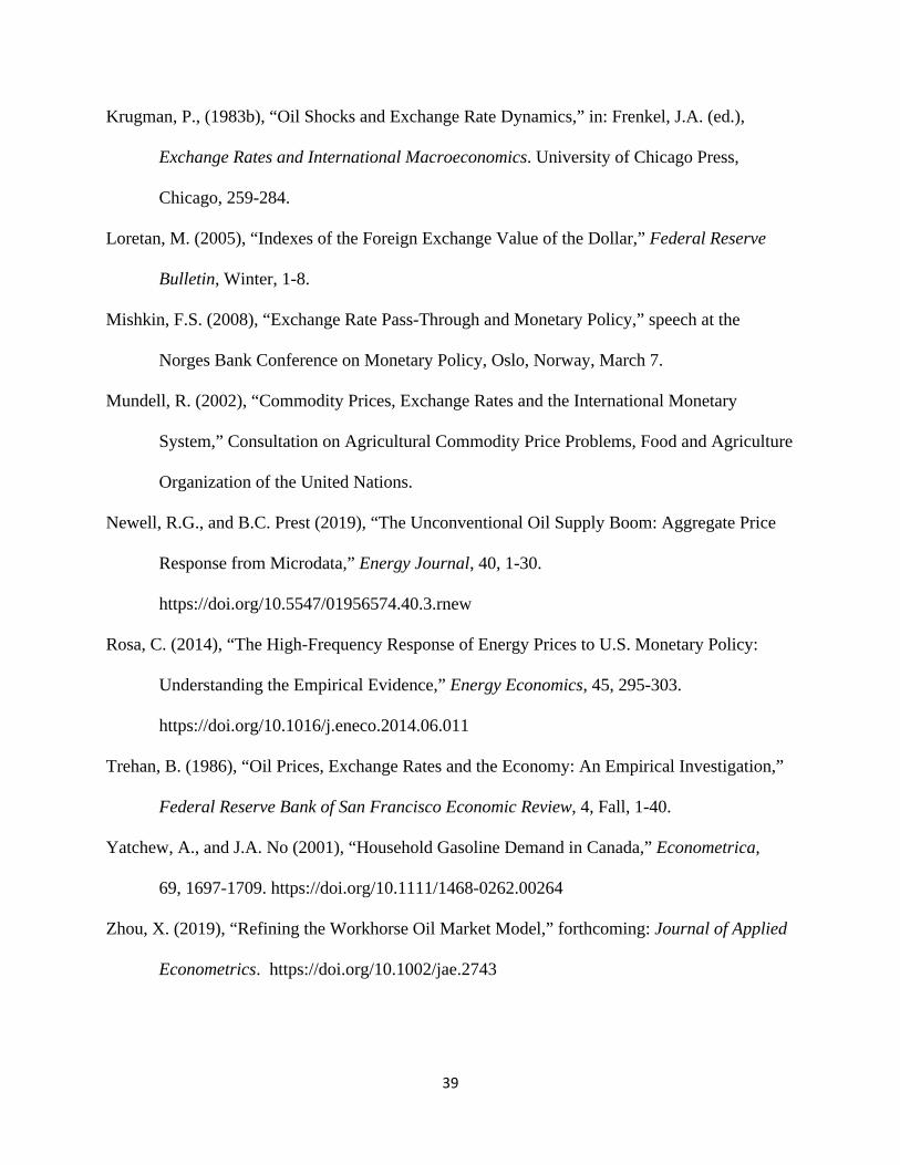
39  

Krugman, P., (1983b), “Oil Shocks and Exchange Rate Dynamics,” in: Frenkel, J.A. (ed.),

Exchange Rates and International Macroeconomics. University of Chicago Press,

Chicago, 259-284.

Loretan, M. (2005), “Indexes of the Foreign Exchange Value of the Dollar,” Federal Reserve

Bulletin, Winter, 1-8.

Mishkin, F.S. (2008), “Exchange Rate Pass-Through and Monetary Policy,” speech at the

Norges Bank Conference on Monetary Policy, Oslo, Norway, March 7.

Mundell, R. (2002), “Commodity Prices, Exchange Rates and the International Monetary

System,” Consultation on Agricultural Commodity Price Problems, Food and Agriculture

Organization of the United Nations.

Newell, R.G., and B.C. Prest (2019), “The Unconventional Oil Supply Boom: Aggregate Price

Response from Microdata,” Energy Journal, 40, 1-30.

https://doi.org/10.5547/01956574.40.3.rnew

Rosa, C. (2014), “The High-Frequency Response of Energy Prices to U.S. Monetary Policy:

Understanding the Empirical Evidence,” Energy Economics, 45, 295-303.

https://doi.org/10.1016/j.eneco.2014.06.011

Trehan, B. (1986), “Oil Prices, Exchange Rates and the Economy: An Empirical Investigation,”

Federal Reserve Bank of San Francisco Economic Review, 4, Fall, 1-40.

Yatchew, A., and J.A. No (2001), “Household Gasoline Demand in Canada,” Econometrica,

69, 1697-1709. https://doi.org/10.1111/1468-0262.00264

Zhou, X. (2019), “Refining the Workhorse Oil Market Model,” forthcoming: Journal of Applied

Econometrics. https://doi.org/10.1002/jae.2743

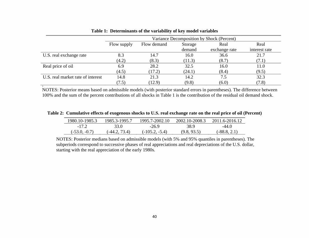
40  

Table 1: Determinants of the variability of key model variables

Variance Decomposition by Shock (Percent) Flow supply Flow demand Storage

demand Real

exchange rate Real

interest rate U.S. real exchange rate 8.3

(4.2) 14.7 (8.3)

16.0 (11.3)

36.6 (8.7)

21.7 (7.1)

Real price of oil 6.9 28.2 32.5 16.0 11.0 (4.5) (17.2) (24.1) (8.4) (9.5) U.S. real market rate of interest 14.8

(7.5) 21.3

(12.9) 14.2 (9.8)

7.5 (6.0)

32.3 (7.8)

()

NOTES: Posterior means based on admissible models (with posterior standard errors in parentheses). The difference between 100% and the sum of the percent contributions of all shocks in Table 1 is the contribution of the residual oil demand shock.

Table 2: Cumulative effects of exogenous shocks to U.S. real exchange rate on the real price of oil (Percent)

1980.10-1985.3 1985.3-1995.7 1995.7-2002.10 2002.10-2008.3 2011.6-2016.12 -17.2 33.0 -26.9 38.9 -44.0

(-53.0, -0.7) (-44.2, 73.4) (-105.2, -5.4) (9.8, 93.5) (-88.8, 2.1)

NOTES: Posterior medians based on admissible models (with 5% and 95% quantiles in parentheses). The subperiods correspond to successive phases of real appreciations and real depreciations of the U.S. dollar, starting with the real appreciation of the early 1980s.

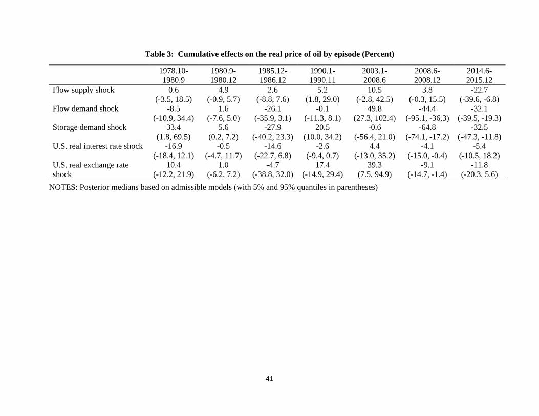
41  

Table 3: Cumulative effects on the real price of oil by episode (Percent)

1978.10-1980.9

1980.9-1980.12

1985.12-1986.12

1990.1-1990.11

2003.1-2008.6

2008.6-2008.12

2014.6-2015.12

Flow supply shock 0.6 4.9 2.6 5.2 10.5 3.8 -22.7 (-3.5, 18.5) (-0.9, 5.7) (-8.8, 7.6) (1.8, 29.0) (-2.8, 42.5) (-0.3, 15.5) (-39.6, -6.8)

Flow demand shock -8.5 1.6 -26.1 -0.1 49.8 -44.4 -32.1 (-10.9, 34.4) (-7.6, 5.0) (-35.9, 3.1) (-11.3, 8.1) (27.3, 102.4) (-95.1, -36.3) (-39.5, -19.3)

Storage demand shock 33.4 5.6 -27.9 20.5 -0.6 -64.8 -32.5 (1.8, 69.5) (0.2, 7.2) (-40.2, 23.3) (10.0, 34.2) (-56.4, 21.0) (-74.1, -17.2) (-47.3, -11.8)

U.S. real interest rate shock -16.9 -0.5 -14.6 -2.6 4.4 -4.1 -5.4 (-18.4, 12.1) (-4.7, 11.7) (-22.7, 6.8) (-9.4, 0.7) (-13.0, 35.2) (-15.0, -0.4) (-10.5, 18.2)

U.S. real exchange rate shock

10.4 1.0 -4.7 17.4 39.3 -9.1 -11.8 (-12.2, 21.9) (-6.2, 7.2) (-38.8, 32.0) (-14.9, 29.4) (7.5, 94.9) (-14.7, -1.4) (-20.3, 5.6)

NOTES: Posterior medians based on admissible models (with 5% and 95% quantiles in parentheses)

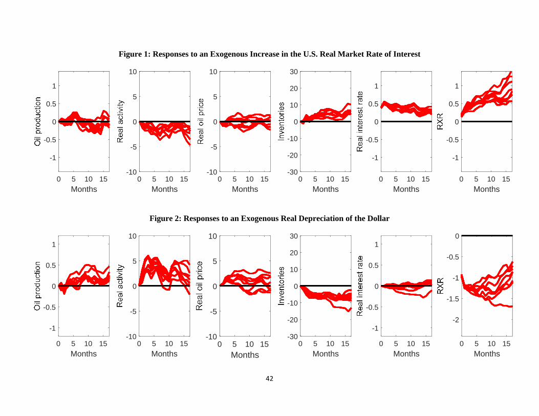
42  

0 5 10 15Months

-1

-0.5

0

0.5

1

0 5 10 15Months

-10

-5

0

5

10

0 5 10 15Months

-10

-5

0

5

10

0 5 10 15Months

-30

-20

-10

0

10

20

30

0 5 10 15Months

-1

-0.5

0

0.5

1

0 5 10 15Months

-1

-0.5

0

0.5

1

0 5 10 15Months

-1

-0.5

0

0.5

1

0 5 10 15Months

-10

-5

0

5

10

0 5 10 15Months

-10

-5

0

5

10

0 5 10 15Months

-30

-20

-10

0

10

20

30

0 5 10 15Months

-1

-0.5

0

0.5

1

0 5 10 15Months

-2

-1.5

-1

-0.5

0

Figure 1: Responses to an Exogenous Increase in the U.S. Real Market Rate of Interest

Figure 2: Responses to an Exogenous Real Depreciation of the Dollar

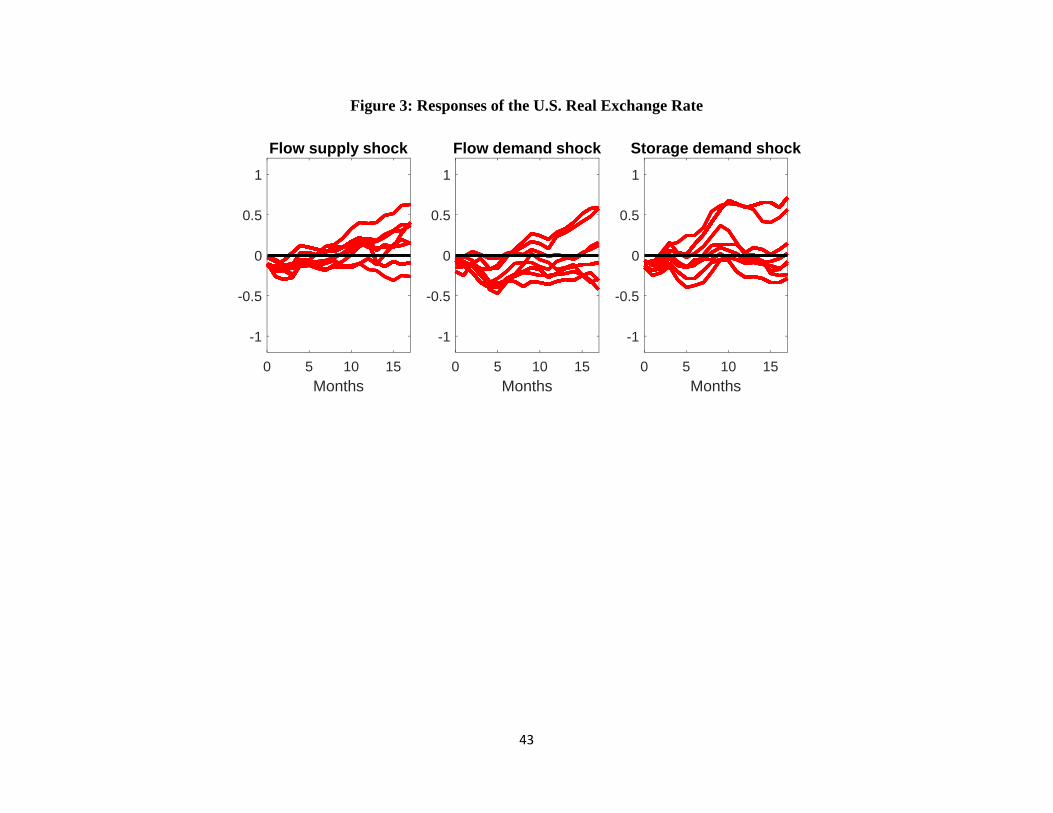
43  

0 5 10 15Months

-1

-0.5

0

0.5

1

Flow supply shock

0 5 10 15Months

-1

-0.5

0

0.5

1

Flow demand shock

0 5 10 15Months

-1

-0.5

0

0.5

1

Storage demand shock

Figure 3: Responses of the U.S. Real Exchange Rate