Oil Shocks through International Transport Costs: Evidence

Federal Reserve Bank of Dallas Globalization and Monetary Policy Institute

Working Paper No. 82 http://www.dallasfed.org/assets/documents/institute/wpapers/2011/0082.pdf

Oil Shocks through International Transport Costs:

Evidence from U.S. Business Cycles*

Hakan Yilmazkuday Florida International University

June 2011

Abstract The effects of oil shocks on output volatility through international transport costs are investigated in an open-economy DSGE model. Two versions of the model, with and without international transport costs, are structurally estimated for the U.S. economy by a Bayesian approach for moving windows of ten years. For model selection, the posterior odds ratios of the two versions are compared for each ten-year window. The version with international transport costs is selected during periods of high volatility in crude oil prices. The contribution of international transport costs to the volatility of U.S. GDP has been estimated as high as 36% during periods of oil crises. JEL codes: E32, E52, F41

* Hakan Yilmazkuday, Department of Economics, Florida International University, Miami, FL 33199. 305-348-2316. [email protected]. The views in this paper are those of the author and do not necessarily reflect the views of the Federal Reserve Bank of Dallas or the Federal Reserve System.

1. Introduction

Figure 1 shows the relation between the U.S. business cycles and the volatility of crude oil prices

for ten-year moving windows. For each ten-year window, the solid line represents the number of

NBER recession quarters, and the dashed line represents the coe¢ cient of variation in oil prices.1

The two series seem to move together with a correlation coe¢ cient of 0.54. This �gure raises the

question of whether oil prices have any signi�cant e¤ects on the business cycles. Many earlier

studies have attempted to answer this question. Among many others, Kim and Loungani (1992)

have shown in a neoclassical model that oil price shocks could explain only a modest component

of the variance of U.S. output growth. Rotemberg and Woodford (1996) have suggested in their

markup pricing model that a 10% increase in energy prices could lead to a 2.5% drop in output after

6 quarters. Finn (2000) has shown that capital utilization is another channel that would provide

similar results as in Rotemberg and Woodford (1996). Bernanke et al. (1997) have claimed that

changes in oil prices lead the Federal Reserve to raise interest rates (in order to control in�ation),

which, in turn, cause downturns; hence, monetary policy is another channel through which oil

prices can a¤ect the business cycles. Similarly, Barsky and Kilian (2002, 2004) have argued that

a monetary expansion was the cause of much of the 1973-74 oil price increase and the decline in

output afterwards. Leduc and Sill (2004) have shown through capital utilization and sticky prices

that monetary policy contributes about 40 percent to the drop in output following a rise in oil

prices. Hamilton and Herrara (2000), Dotsey and Reid (1992), Hoover and Perez (1994), Ferderer

(1996), Brown and Yücel (1999), and Davis and Haltiwanger (2001) have all shown empirically

that, compared to the monetary policy, the oil prices have been more in�uential on the business

1Business cycle dates have been obtained from http://www.nber.org/cycles.html. Crude oil prices have been

obtained from http://www.ioga.com.

2

cycles. Bresnahan and Ramey (1993), Bohi (1991), Lee and Ni (2002), Davis and Haltiwanger

(2001), and Keane and Prasad (1996) have focused on the frictions in reallocating labor or capital

across di¤erent sectors that may be di¤erentially a¤ected by an oil shock.

This paper mostly belongs to the part of the literature that focuses on the e¤ects of oil price

shocks on the business cycles through the CPI in�ation rate. As Hamilton (2005) nicely puts, the

in�ation rate is governed by monetary policy, so, ultimately, this is a question about how the central

bank responds to the oil price shock. Hooker (2002) has found evidence that oil shocks made a

substantial contribution to U.S. core in�ation before 1981 but have made little contribution since,

consistent with the conclusion of Clarida, Galí and Gertler (2000) that U.S. monetary policy has

become signi�cantly more devoted to curtailing in�ation. Within this picture (i.e., the e¤ects of oil

prices on the business cycles through the in�ation rate), none of the papers mentioned above have

investigated the international-transport-cost channel of oil prices. In particular, in a world where

consumer utility depends on domestically-produced goods and internationally-imported goods, the

in�ation rate depends on the price of domestically-produced goods and the price of internationally-

imported goods that includes international transport costs. A natural question arises: What are

the e¤ects of oil price shocks on the business cycles through international price di¤erences (i.e.,

short-term deviations from the Law of One Price) measured by such international transport costs?

This paper attempts to answer this question by estimating two versions of a standard DSGEmodel,

with and without international transport costs, using the U.S. quarterly data. In the version with

transport costs, the optimization of individuals and �rms in a �exible price equilibrium setup

result in having the e¤ects of international transport costs in the IS equation, the Phillips curve,

the terms of trade expression, the monetary policy rule, and the CPI in�ation rate. The structural

estimation is achieved by a Bayesian approach for each ten-year window between 1957-2010 to

investigate nonlinearities in the U.S. economy caused by oil price shocks through time. For each

3

ten-year window, the posterior odds ratios of the two versions of the model are compared for

model selection. The results suggest that a necessary condition for the version of the model with

transport costs to be selected is to have a coe¢ cient of variation in crude oil prices of above 0.25

over a ten-year period. Although the average contribution of international transport costs to the

volatility of U.S. GDP is estimated about 3% for the whole sample period, the contribution is up

to 36% during periods of oil crises. According to the structural estimation results, the Federal

Reserve has used interest rates as a policy tool during periods of oil crises mostly to stabilize

output rather than the in�ation rate or the interest rate.

The rest of the paper is organized as follows. Section 2 gives a summary of the model. Section

3 introduces the data and the estimation methodology. Section 4 depicts the estimation results.

Section 5 concludes. The detailed derivation of the model, together with its implications, is given

in the Appendices.

2. Model

The model is a version of Gali and Monacelli (2005) with the addition of international transport

costs at the �nal goods level. The model consists of a forward-looking IS-equation and a forward-

looking Phillips curve, together with a monetary policy described by an interest rate rule and a

terms-of-trade expression. The detailed derivation of model is given in Appendix A.

The IS curve is given by

yt = Et (yt+1)� (it � Et (�H;t+1)) + Et (�� t+1)

where yt is the output, it is the annual nominal interest rate, �H;t is the annual in�ation of home-

produced goods, � t represents symmetric transport costs on internationally traded (i.e., both

exported and imported) �nal goods, Et is the expectation operator, and � is the �rst-di¤erence

4

operator.

The Phillips curve is given by

�H;t = �Et (�H;t+1) + �xxt

where �x =(1��)(1��)

�, � is the probability that a �rm does not change its price within a given

period (i.e., price stickiness), � is the discount factor, xt � yt � zt + � t represents the output gap

under a �exible price equilibrium where zt is the level of technology. As is shown in Appendix

B, stabilizing the output gap (the gap between actual and natural output) is not equivalent to

stabilizing the welfare-relevant output gap (the gap between actual and e¢ cient output). Hence,

there is no divine coincidence in the model of this paper mentioned by Blanchard and Gali (2007).

The nominal interest rates are determined by a Taylor rule:

it = (1� �i) (��Et (�t+1) + �xEt (xt)) + �iit�1 + "t

where �t is the annual consumer price index (CPI) in�ation, �i captures the degree of interest-rate

smoothing, and "t is an exogenous policy shock which can be interpreted as the non-systematic

component of monetary policy. The relation between in�ation of home-produced goods (i.e., �H;t)

and CPI in�ation (i.e., �t) is given by:

�t = �H;t + (�st)

where is a measure of openness, and st is the e¤ective terms of trade given by:

st =�i�t � Et

��F;t+1

�� (it � Et (�H;t+1)) + Et (st+1 �� t+1)

where i�t is the annual foreign interest rate, and ��F;t is the annual foreign in�ation (through

imported goods). Since i�t and ��F;t appear only in the terms of trade expression, we will combine

them under a foreign �nancial variable, f �t = i�t � Et

��F;t+1

�.

5

There are three additional independent shocks considered in the model, namely technology,

international transport costs, and foreign �nancial variable:

zt = �zzt�1 + vzt

� t = �� t�1 + v�t

f �t = �f�f�t�1 + v

f�

t

As is evident, there is no foreign output variable (hence no foreign output shock) in the model.

Instead, as shown in Appendix C, the expected change in foreign output is decomposed into the

foreign �nancial variable and transport costs. As discussed in Appendix D, the foreign �nancial

variable also captures any international �nancial frictions or shocks between home and foreign

countries through the exogenous foreign interest rate. Hence, one may expect to have higher

contributions of the foreign �nancial variable and international transport costs on the business

cycles, because they may capture such latent variables mentioned above.

As opposed to this paper, many studies have endogenized the deviations from the Law of One

price; e.g., Monacelli (2005) has introduced a model with import retailers subject to price rigidities

of which versions have been estimated by many studies such as Lubik and Schorfheide (2005) for

the Euro Area, Justiniano and Preston (2010) for Canada, Australia and New Zealand, Adolfson

et al. (2007) for Sweden; similarly, Gust et al. (2009) have focused on local currency assumptions,

non-constant elasticity of demand, or distribution costs; Bridgman (2008) has introduced a model

with transportation sector to investigate the expansion of world trade. Nevertheless, the exogeneity

of international transport costs is simple and enough for the question asked in this paper, because

we only care about the exogenous e¤ects of oil shocks on the U.S. business cycles.

6

3. Data and Estimation Methodology

The open-economy model is estimated using data on the U.S. economy obtained from International

Financial Statistics for the quarterly period over 1957:Q1-2010:Q4. The variables are calculated

as percentage deviations from their steady-states to take care of any possible stationarity issues.

We use observations on the percentage deviations of real output, CPI in�ation, and short-term

nominal interest rates from their steady states in annual terms where percentage deviations have

been calculated as Hodrick-Prescott �ltered versions of seasonally adjusted Real GDP (US$ at

2005 prices), Consumer price index (2005=100), and Federal Funds Rate.

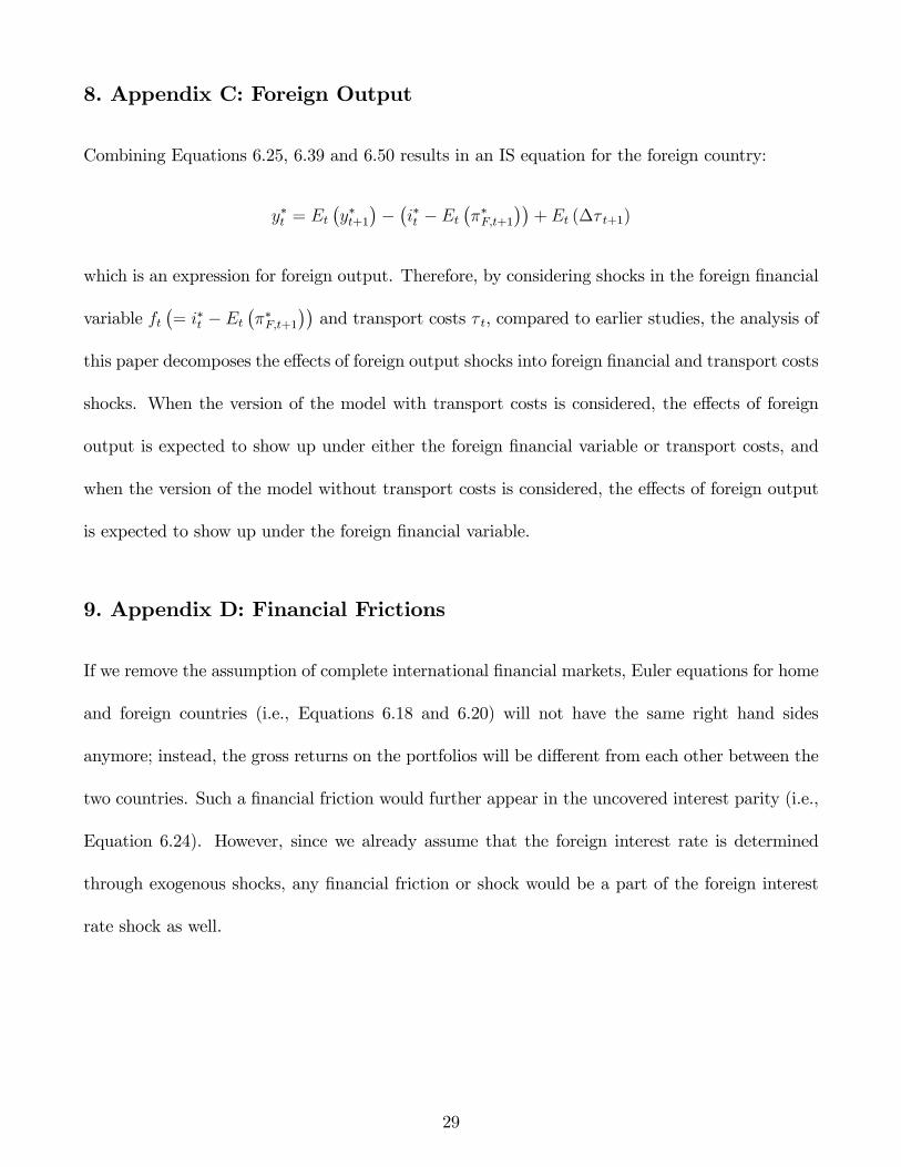
The estimation is achieved through a Bayesian approach where the choice of priors for the

structural parameters plays an important role. Table 1 provides information on prior distributions

for all parameters that have been selected as consistent with the existing literature (e.g., see Lubik

and Schorfheide, 2007, An and Schorfheide, 2007, and the discussions therein). One important

detail is that the model is parameterized in terms of the steady-state real interest rate r, rather

than the discount factor �, where r is annualized such that � = exp (�r=400).

The moving-window estimation is achieved for each ten-year period between 1957:Q1-2010:Q4.

To address the question of whether international transport costs are signi�cant in explaining output

volatilities, for each ten-year period, two versions of the model, with (� t > 0 for all t) and without

(� = 0 for all t) transport costs, are estimated. For model selection, we assess the hypothesis of

� = 0 against the alternative of � t > 0 for all t by computing the posterior odds ratios for each

ten-year period. The reader is referred to Lubik and Schorfheide (2007) for technical details related

to the calculation of the posterior odds ratio.

7

4. Estimation Results

4.1. Model Selection

Figure 2 shows the selected version of the model (i.e., with or without trade costs) versus the

volatility in oil prices for each ten-year period estimated. While the vertical axis on the left shows

the volatility in oil prices (measured by the coe¢ cient of variation), the vertical axis on the right

shows the selected model by taking a value of 0 for the version of the model with � t = 0 and

a value of 1 for the version of the model with � t > 0. As is evident, the model with positive

international transport costs shocks has been selected during periods of high oil price volatility

that include the production peak of the U.S. in 1970, the oil crises in 1973 and 1979, the oil glut

in 1980s, the 1990 oil price spike occurred in response to the Iraqi invasion of Kuwait, and the

2005 oil price shock. One striking evidence is that a necessary condition for the version of the

model with positive international transport costs shocks to be selected is to have a coe¢ cient of

variation in crude oil prices above 0.25. Therefore, according to the methodology of this paper

and the relation between oil prices and recessions in Figure 1, the U.S. GDP has been a¤ected by

international transport costs during period of high oil price volatility. But, how important are these

international transport costs? To answer this question, we calculate the variance decomposition

of the U.S. GDP for each ten-year window, below.

4.2. Variance Decomposition of Output

The variance decomposition of the U.S. GDP through the version of the model with international

transport costs (i.e., � t > 0) is given in Figure 3. According to this version of the model, on average,

about 30% of output volatility is due to transport costs shocks, 47% due to foreign �nancial shocks,

13% due to technology shocks, and 10% due to monetary policy shocks. High contributions of

8

international shocks, namely transport costs and foreign �nancial shocks, are mostly attributable

to latent variables of foreign output (see Appendix C) and �nancial frictions (see Appendix D)

that show up under either of these two shocks. One striking evidence is that, during the periods of

oil crises, the e¤ect of transport costs falls, and the e¤ects of foreign �nancial and monetary policy

shocks increase. Hence, the e¤ects of oil shocks are mostly through international �nancial markets

or the monetary policy rather than the direct e¤ects of oil prices on international transport costs.

Another evidence is that technology shocks have a higher contribution on output volatility starting

from mid-1980s.

The variance decomposition of the U.S. GDP through the version of the model without interna-

tional transport costs (i.e., � t = 0) is given in Figure 4. According to this version of the model, on

average, 63% of output volatility is due to foreign �nancial shocks, 13% due to technology shocks,

and 24% due to monetary policy shocks. Hence, the e¤ect of transport costs on output volatility

in the version with transport costs seems to be mostly replaced by either the foreign �nancial

variable or the monetary policy in the version without transport costs. During the periods of oil

crises, the e¤ect of foreign �nancial shocks seems to be higher. Hence, the e¤ects of oil shocks are

mostly through international �nancial markets in this version of the model. As in the model with

transport costs, technology shocks have a higher contribution on output volatility starting from

mid-1980s.

When we turn back to our question of how important international transport costs are, we

combine the variance decompositions of output coming from the two versions of the model. In

particular, we know which model is selected by the posterior odds ratio for each ten-year window;

by using the variance decomposition of output obtained from the selected model for each ten-year

window, we combine the variance decompositions of output in Figure 5. As is evident, international

transport costs can contribute to the volatility of output up to 36% during the periods of oil crises.

9

Nevertheless, the average contribution of international transport costs on the volatility of output

is about 3% for the whole sample period; this latter result is consistent with Kim and Loungani

(1992) who have shown in a neoclassical model that oil price shocks could explain only a modest

component of the variance of U.S. output. In sum, although the e¤ect of international transport

costs is minimal during non-crisis periods, the U.S. economy has had experienced signi�cant e¤ects

of oil prices on its output through international transport costs during the periods of oil crises.

According to the combined variance decomposition of output, on average, the contributions

of foreign �nancial variable shock, monetary policy shock, technology shock, and international

transport shock are 62%, 23%, 12%, and 3%, respectively, for the whole sample period. Therefore,

the direct e¤ects of oil price changes through international transport costs are less than the e¤ects

of monetary policy shocks; this result is opposed to studies such as Hamilton and Herrara (2000),

Dotsey and Reid (1992), Hoover and Perez (1994), Ferderer (1996), Brown and Yücel (1999), and

Davis and Haltiwanger (2001), and it is consistent with studies such as Bernanke et al. (1997),

Barsky and Kilian (2002, 2004), and Leduc and Sill (2004). Nevertheless, the biggest e¤ect on

output is due to foreign �nancial shocks which may have also been a¤ected by oil price shocks in an

indirect way (e.g., the e¤ects of oil shocks on the rest of the world). Once again, high contributions

of international shocks, namely transport costs and foreign �nancial shocks, are mostly attributable

to latent variables of foreign output (see Appendix C) and �nancial frictions (see Appendix D)

that show up under either of these two shocks.

4.3. Monetary Policy

The other parameters of the model (i.e., the posterior means as point estimates) have also been

obtained through the ten-year window estimations. To save space and focus on the monetary policy

through time, we only depict the Taylor rule parameter estimates obtained from the combination

10

of the two versions of the model; i.e., each depicted parameter belongs to the model selected by

the posterior odds ratio. The estimates of �� through time are given in Figure 6. As is evident,

the response of the Federal Reserve to the deviations of in�ation from its target value seems to

be negatively related to the volatility of crude oil prices; in other words, during the periods of

oil crises, the Federal Reserve has given fewer weight to in�ation according to our Taylor rule

speci�cation. The estimates of �x through time are given in Figure 7. As is evident, the response

of the Federal Reserve to the deviations of output from its �exible-price-equilibrium value seems

to be positively related to the volatility of crude oil prices; hence, during the periods of oil crises,

which mostly correspond to the recession periods according to Figure 1, the Federal Reserve has

given more weight to output gap according to our Taylor rule speci�cation. The estimates of �i

through time are given in Figure 8 where, as one would expect from an active monetary policy,

the interest-rate smoothing is fewer during the times of crises. The last three results suggest that

the Federal Reserve has used interest rates as a policy tool during oil crises periods mostly to

stabilize output rather than the in�ation rate or the interest rate; hence, the Federal Reserve has

used interest rates as a policy tool during non-crisis periods mostly to stabilize the in�ation rate

and the interest rate.

5. Conclusion

Two versions of a standard DSGE model, with and without international transport costs, have

been estimated by Bayesian techniques to investigate possible e¤ects of oil price shocks on the U.S.

business cycles through international transport costs. The estimation has been achieved for each

ten-year window between 1957-2010 to investigate nonlinearities in the U.S. economy caused by oil

price shocks through time. A necessary condition for the version of the model with positive inter-

11

national transport costs shocks to be selected is to have a coe¢ cient of variation in crude oil prices

above 0.25 over a ten-year period. Although the average contribution of international transport

costs to the volatility of U.S. GDP is about 3% for the whole sample period, the contribution is

up to 36% during periods of oil crises. The Federal Reserve has used interest rates as a policy tool

during periods of oil crises mostly to stabilize output rather than the in�ation rate or the interest

rate and vice versa.

The results of this paper should be quali�ed with respect to the structural model employed as it

may be misspeci�ed. The results are subject to further improvement; endogenizing transport costs

through an oil producing sector/country, introducing capital accumulation, di¤erent production

sectors, intermediate input trade, and internationally incomplete asset markets would generate

richer model dynamics. These are possible topics of future research.

References

[1] Adolfson, M., J. Linde, M. Villani, (2007), "Forecasting Performance of an Open Economy

DSGE Model", Econometric Reviews, 26, 289-328.

[2] An, S. and Schorfheide, F., (2007), "Bayesian Analysis of DSGE Models," Econometric Re-

views, 26: 113-172.

[3] Barsky, Robert B., and Lutz Kilian (2002). �Do We Really Know that Oil Caused the Great

Stag�ation? A Monetary Alternative,� in Ben S. Bernanke and Ken Rogo¤, eds., NBER

Macroeconomics Annual 2001, MIT Press: Cambridge, MA, pp. 137-183.

[4] Barsky, Robert B., and Lutz Kilian (2004). �Oil and the Macroeconomy Since the 1970s,�

Journal of Economic Perspectives 18, no. 4, pp. 115-134.

12

[5] Bernanke, Ben S., Mark Gertler, and MarkWatson (1997), �Systematic Monetary Policy and

the E¤ects of Oil Price Shocks,�Brookings Papers on Economic Activity, 1-1997, pp. 91-124.

[6] Blanchard, Olivier and Jordi Gali (2007). "Real Wage Rigidities and the New Keynesian

Model," Journal of Money, Credit and Banking, Volume 39, pages 35�65.

[7] Bohi, Douglas R. (1991), �On the Macroeconomic E¤ects of Energy Price Shocks,�Resources

and Energy, 13, pp. 145-162

[8] Bresnahan, Timothy F., and Valerie A. Ramey (1993), �Segment Shifts and Capacity Utiliza-

tion in the U.S. Automobile Industry,�American Economic Review Papers and Proceedings,

83, no. 2, pp. 213-218.

[9] Bridgman, B., (2008), "Energy prices and the expansion of world trade", Review of Economic

Dynamics, 11, 904-916.

[10] Brown, Stephen P.A., and Mine K. Yücel (1999), �Oil Prices and U.S. Aggregate Economic

Activity: A Question of Neutrality,�Economic and Financial Review, Federal Reserve Bank

of Dallas, (Second Quarter), pp. 16-23.

[11] Clarida, Richard, Jordi Galí, and Mark Gertler (2000), �Monetary Policy Rules and Macro-

economic Stability: Evidence and Some Theory,�Quarterly Journal of Economics, 115. pp.

147-180.

[12] Davis, Steven J., and John Haltiwanger (2001), �Sectoral Job Creation and Destruction Re-

sponses to Oil Price Changes,�Journal of Monetary Economics, 48, pp. 465-512.

[13] Dotsey, Michael, and Max Reid (1992), �Oil Shocks, Monetary Policy, and Economic Activ-

ity,�Economic Review of the Federal Reserve Bank of Richmond, 78/4, pp. 14-27.

13

[14] Ferderer, J. Peter (1996), �Oil Price Volatility and the Macroeconomy: A Solution to the

Asymmetry Puzzle,�Journal of Macroeconomics, 18 (1996), pp. 1-16.

[15] Finn, Mary G. (2000), �Perfect Competition and the E¤ects of Energy Price Increases on

Economic Activity,�Journal of Money, Credit, and Banking, 32, pp. 400-416.

[16] Gali, Jordi. and Tomasso Monacelli (2005), �Monetary Policy and Exchange Rate Volatility

in a Small Open Economy�, Review of Economic Studies, 72: 707-734.

[17] Gust, C., S. Leduc, N. Sheets (2009), "The adjustment of global external balances: Does par-

tial exchange-rate pass-through to trade prices matter?", Journal of International Economics,

79, 173-185.

[18] Hamilton, J.D. (2005), �Oil and the Macroeconomy,�forthcoming in S. Durlauf and L. Blume

(eds), The New Palgrave Dictionary of Economics, 2nd ed., Palgrave MacMillan Ltd.

[19] Hansen, Gary D., (1985). "Indivisible labor and the business cycle," Journal of Monetary

Economics, vol. 16(3), pages 309-327.

[20] Hooker, Mark A. (2002), �Are Oil Shocks In�ationary? Asymmetric and Nonlinear Speci�ca-

tions versus Changes in Regime,�Journal of Money, Credit and Banking 34, pp. 540-561.

[21] Hoover, Kevin D., and Stephen J. Perez (1994), �Post Hoc Ergo Propter Once More: An

Evaluation of �Does Monetary Policy Matter?� in the Spirit of James Tobin,� Journal of

Monetary Economics, 34, pp. 89-99.

[22] Justiniano, A., B. Preston, (2010), "Monetary Policy and Uncertainty in an Empirical Small

Open-Economy Model", Journal of Applied Econometrics, 25, 93-128.

14

[23] Keane, Michael P., and Eswar Prasad (1996), �The Employment and Wage E¤ects of Oil

Price Changes: A Sectoral Analysis,�Review of Economics and Statistics, 78, pp. 389-400.

[24] Kerr, W., and King, R.G., (1996), �Limits on interest rate rules in the IS model�, Federal

Reserve Bank of Richmond Economic Quarterly 82: 47-75.

[25] Kim, In-Moo, and Prakash Loungani (1992), �The Role of Energy in Real Business Cycle

Models,�Journal of Monetary Economics, 29, no. 2, pp. 173-189.

[26] King, R.G., (2000), �The New IS-LM Model: Language, Logic and Limits�, Federal Reserve

Bank of Richmond Economic Quarterly Volume 86/3.

[27] Leduc, Sylvain and Keith Sill (2004), �AQuantitative Analysis of Oil-Price Shocks, Systematic

Monetary Policy, and Economic Downturns,�Journal of Monetary Economics, 51, pp. 781-

808.

[28] Lee, Kiseok, and Shawn Ni (2002), �On the Dynamic E¤ects of Oil Price Shocks: A Study

Using Industry Level Data,�Journal of Monetary Economics, 49, pp. 823-852.

[29] Lubik, T.A., Schorfheide, F., (2005), A Bayesian look at NewOpen EconomyMacroeconomics.

NBER Macroeconomics Annual 20, 313� 366.

[30] Lubik, T.A. and Schorfheide, F., (2007), �Do Central Banks Respond to Exchange Rate

Movements: A Structural Investigation�, Journal of Monetary Economics, 54: 1069-1087.

[31] Monacelli, T., (2005), "Monetary Policy in a Low Pass-Through Environment", Journal of

Money Credit and Banking, vol 37, 1047-1066.

[32] Rotemberg, Julio J., and Michael Woodford (1996), �Imperfect Competition and the E¤ects

of Energy Price Increases,�Journal of Money, Credit, and Banking, 28 (part 1), pp. 549-577.

15

[33] Rotemberg, Julio J., and Michael Woodford (1999), �Interest Rate Rules in an Estimated

Sticky Price Model�, in J. B. Taylor (ed.) Monetary Policy Rules (Chicago: University of

Chicago Press).

[34] Yilmazkuday, Hakan, (2009), �Is there a Role for International Trade Costs in Explaining the

Central Bank Behavior�, MPRA Working Paper No 15951.

6. Appendix A: Derivation of the Model

The model is a modi�ed and simpler version of Gali and Monacelli�s (2005) open-economy model

with the addition of international transport costs as presented in Yilmazkuday (2009).2 It is

a continuum of goods model in which all goods are tradable, the representative individual holds

assets, and the production of goods requires labor input. SubscriptsH and F stand for domestically

and foreign-produced goods, respectively. Superscript � stands for the variables of the foreign

country (i.e., rest of the world). A bar on a variable ( : ) stands for a target value. Lower case

letters denote log variables. Capital letters without a time subscript denote steady-state values.

6.1. Individuals

The representative individual in the domestic (i.e., home) country has the following intertemporal

lifetime utility function:

Et

" 1Xk=0

�k fU (Ct+k)� V (Nt+k)g#

(6.1)

where U (Ct) is the utility out of consuming a composite index of Ct, V (Nt) is the disutility out

of working Nt hours, and 0 < � < 1 is a discount factor. The composite consumption index Ct is

2The model of this paper slightly deviates from Yilmazkuday (2009) by assuming a zero-trend in�ation, because

all variables are represented as percentage deviations from their steady-states in this paper.

16

de�ned by:

Ct = (CH;t)1� (CF;t)

(6.2)

where CH;t and CF;t are consumption of home and foreign (i.e., imported) goods, respectively, and

is the share of domestic consumption allocated to imported goods. These symmetric consumption

sub-indexes are de�ned by:

CH;t =

�Z 1

0

CH;t(j)(��1)=�dj

��=(��1)and CF;t =

�Z 1

0

CF;t(j)(��1)=�dj

��=(��1)(6.3)

where CH;t(j) and CF;t(j) represent domestic consumption of home and foreign good j, respectively,

and � > 1 is the price elasticity of demand faced by each monopolist. The optimality conditions

result in:

CH;t(j) =hPH;t(j)

PH;t

i��CH;t

CF;t(j) =hPF;t(j)

PF;t

i��CF;t

(6.4)

where PH;t(j) and PF;t(j) are prices of domestically consumed home and foreign good j, respec-

tively. PH;t and PF;t are price indexes of domestically consumed home and foreign goods, respec-

tively, which are de�ned as:

PH;t =

�Z 1

0

([PH;t(j)])1�� dj

�1=(1��)(6.5)

and

PF;t =

�Z 1

0

([PF;t(j)])1�� dj

�1=(1��)(6.6)

Similarly, the demand allocation of home and imported goods implies:

CH;t =(1� )CtPt

PH;t(6.7)

and

CF;t = PtCtPF;t

(6.8)

17

where Pt =�PH;t

�1� �PF;t

� is the consumer price index (CPI). The log-linear version of CPI can

be written as:

pt � (1� )pH;t + pF;t (6.9)

where pH;t and pF;t are logs of PH;t and PF;t, respectively. The (log) price index for imported goods

is further given by:

pF;t = et + p�F;t + � t (6.10)

where et is the (log) nominal e¤ective exchange rate; p�F;t is the (log) price index of domestically

consumed foreign goods at the source; and � t is the (log) gross international transport cost, which

is an income received by the rest of the world.3 The (log) gross international transport cost directly

enters the price index for imported goods, because it is assumed that the international transport

costs are the same across goods, and they are symmetric. The evolution of international transport

costs is given by an AR(1) process:

� t = �� t�1 + "�t (6.11)

where �� 2 [0; 1] and "�t is assumed to be an independent and identically distributed (i.i.d.) shock

with zero mean and variance �2� .

The (log) e¤ective terms of trade is de�ned as st � pF;t�pH;t, which implies that the (log) CPI

formula can be written as:

pt � (1� )pH;t + pF;t (6.12)

Combining st � pF;t� pH;t and pF;t = et+ p�F;t+ � t results in an alternative expression for the (log)3For future reference, p�H;t is the (log) price index for the imported goods for the rest of the world, and p

�F;t is

the (log) domestic price index for the rest of the world. We assume that the trade costs consist of transportation

costs and transportation sector is owned by the rest of the world, so there is no transportation income received by

the home country.

18

e¤ective terms of trade:

st � et + p�F;t + � t � pH;t (6.13)

which includes international transport costs.

The formula of CPI in�ation follows as:

�t = �H;t + (st � st�1) (6.14)

where �t = pt�pt�1 is CPI in�ation, and �H;t = pH;t�pH;t�1 is the in�ation of home-produced goods

(i.e., home in�ation). Combining Equations 6.13 and (6.14) results in an alternative expression of

CPI in�ation:

�t = (1� )�H;t + ��F;t +�et +�� t

�(6.15)

which suggests that CPI in�ation is a weighted sum of home in�ation, foreign in�ation, growth in

exchange rate, and growth in international transport costs. Hence, international transport costs

play an important role in the determination of CPI in�ation.

The individual household constraint is given by:

Z 1

0

[PH;t(j)CH;t(j) + PF;t(j)CF;t(j)] dj + Et [Ft;t+1Bt+1] =WtNt +Bt + Tt (6.16)

where Ft;t+1 is the stochastic discount factor, Bt+1 is the nominal payo¤ in period t + 1 of the

portfolio held at the end of period t,Wt is the hourly wage, and Tt is the lump sum transfers/taxes.

By using the optimal demand functions, Equation (6.16) can be written in terms of the com-

posite good as follows:

PtCt + Et [Ft;t+1Bt+1] =WtNt +Bt + Tt (6.17)

The representative home agent�s problem is to choose paths for consumption, portfolio, and the

labor supply. Therefore, the representative consumer maximizes her expected utility [equation

19

(6.1)] subject to the budget constraint [equation (6.17)]. The �rst order condition implies that:

�Et

�UC(Ct+1) PtUC(Ct) Pt+1

�=1

It(6.18)

where It = 1/Et [Ft;t+1] is the gross return on the portfolio. Equation (6.18) represents the tradi-

tional intertemporal Euler equation for total real consumption. The labor supply decision of the

individual is obtained as follows:

Wt

Pt=VN (Nt)

UC (Ct)(6.19)

The problem is analogous for the rest of the world: Euler equation for the rest of the world is given

by:

�Et

�u�C(C

�t+1)P

�t �t

u�C(C�t ) P

�t+1�t+1

�= Et [Ft;t+1] (6.20)

where �t is the nominal e¤ective exchange rate. Combining Equations (6.18) and (6.20), together

with assuming U(Ct) = logCt, one can obtain:

Ct = C�tQt (6.21)

for all t, where Qt = �tP�t =Pt is the real e¤ective exchange rate; thus, the (log) e¤ective real

exchange rate is obtained as:

qt = et + p�t � pt (6.22)

By using Equations (6.9), (6.10) and (6.13), together with the symmetric versions of Equations

(6.9) and (6.10) for the rest of the world, we can rewrite Equation (6.22) as follows:

qt = (1� � �)st � (1� 2 �)� t (6.23)

where � is the share of foreign consumption allocated to goods imported from the home country.

Under the assumption of complete international �nancial markets, by combining log-linearized

version of Equations (6.18), (6.20) and (6.21), together with Equation (6.22), the uncovered interest

20

parity condition is obtained as:

it = i�t + Et [et+1]� et (6.24)

where it = log (It) = log (1/ (Et [Ft;t+1])) is the home interest rate and i�t = log (�t/ (Et [Ft;t+1�t+1]))

is the foreign interest rate. This uncovered interest parity condition relates the movements of the

interest rate di¤erentials to the expected variations in the e¤ective nominal exchange rate. Since

st � et + p�F;t + � t � pH;t according to Equation (6.13), we can rewrite Equation (6.24) as follows:

st =�i�t � Et

��F;t+1

��it � Et

��H;t+1

��+ Et

�st+1 �� t+1

�(6.25)

where �� t+1 is the change in trade cost from period t to t + 1. Equation (6.25) shows the terms

of trade between the home country and the rest of the world as a function of current interest

rate di¤erentials, expected future home in�ation di¤erentials and its own expectation for the next

period together with the expected future change in trade cost. Here, the evolution of foreign

interest rate shock is given by:

i�t = �i�i�t�1 + "

i�

t (6.26)

where �i� 2 [0; 1], and "i�t is assumed to be an independent and identically distributed (i.i.d.) shock

with zero mean and variance �2i�.

6.2. Firms

The representative domestic �rm has the following production function:

Yt (j) = ZtNt (j) (6.27)

where Zt is an exogenous economy-wide productivity parameter; and Nt is labor input. Accord-

ingly, the marginal cost of production is given by:

MCnt = (1� !)Wt

Zt(6.28)

21

where ! is the employment subsidy. The inclusion of this subsidy is not arbitrary, because as

discussed below, under the assumption of a constant employment subsidy ! that neutralizes the

distortion associated with �rms�market power, it can be shown that the optimal monetary policy

is the one that replicates the �exible price equilibrium allocation in a closed economy.

Using Equation (6.19), together with assuming V (Nt) = Nt, the log-linearized real marginal

cost can be written as follows:4

mct = log (1� !) + wt � pH;t � zt (6.29)

Moreover, if the aggregate output in the home country is de�ned as Yt =hR 10Yt(j)

(��1)=�dji�=(��1)

,

labor market equilibrium implies:

Nt =

Z 1

0

Nt(j)dj =YtAtZt

(6.30)

where At =R 10Yt(j)Ytdj of which equilibrium variations can be shown to be of second-order in log

terms. Thus, in �rst-order log-linearized terms, we can write:

yt = zt + nt (6.31)

where zt evolves according to:

zt = �zzt�1 + "zt (6.32)

where �z 2 [0; 1] and "zt is assumed to be an i.i.d. shock with zero mean and variance �2z.

6.3. Market Clearing

For all di¤erentiated goods, market clearing implies:

Yt(j) = CH;t(j) + C�H;t(j) (6.33)

4Balanced growth requires the relative risk aversion in consumption to be unity, and thus we set U(C) = logC

. Following the lead of Hansen (1985), we also assume that labor is indivisible, implying that the representative

agent�s utility is linear in labor hours so that V (N) = N .

22

Using Equation (6.4), it can be rewritten as follows:

Yt(j) =

�PH;t(j)

PH;t

��CAH;t (6.34)

where CAH;t = CH;t + C�H;t is the aggregate world demand for the goods produced in the home

country. Using Equation (6.7) and the symmetric version of Equation (6.8) for the rest of the

world, Equation (6.34) can be rewritten as follows:

Yt(j) =

�PH;t(j)

PH;t

�� (1� )PtCt

PH;t+ �

P �t C�t

P �H;t

!(6.35)

Using Yt =hR 10Yt(j)

(��1)=�dji�=(��1)

, one can write:

Yt =�(1� )PtCt

PH;t+ �

P �t C�t

P �H;t

�=

�PtPH;t

�Ct

�(1� ) + �

�P �t PH;tPtP �H;t

�Q�1t

� (6.36)

which implies that Equation (6.35) can be rewritten as follows:

Yt(j) =

�PH;t(j)

PH;t

��Yt (6.37)

Log-linearizing Equation (6.36) around the steady-state, together with using st � pF;t � pH;t and

Equation (6.23), will transform it to the following expression:

yt = ct + st � � t (6.38)

Also using Equation (6.14) and the log-linearized version of Equation (6.18) (i.e., Euler), Equation

(6.38) can be rewritten as follows:

yt = Et (yt+1)��it � Et

��H;t+1

��+ Et (�� t+1) (6.39)

which represents an IS curve that considers the e¤ect of international transport costs on output,

which is not the usual case in the literature where the last term (i.e., the expected change in

international transport costs) is absent. From another point of view, Equation (6.39) represents

23

an IS curve that relates the expected change in (log) output (i.e., Et (yt+1)� yt) to the di¤erence

between the interest rate, the expected future domestic in�ation (i.e., an approximate measure of

real interest rate that becomes an exact measure of real interest rate when the terms of trade are

constant across periods), and the expected change in international transport costs.5 An increase in

the di¤erence between the expected in�ation and the nominal interest rate decreases the expected

change in the output gap, with a unit coe¢ cient. Finally, an expected increase in the international

transport costs leads to a decrease in the expected change in (log) output. The latter is due to the

intertemporal substitution of supply in response to a change in international transport costs.

The model employs a Calvo price-setting process, in which producers are able to change their

prices only with some probability, independently of other producers and the time elapsed since the

last adjustment. It is assumed that producers behave as monopolistic competitors. Accordingly,

each producer faces the following demand function:

Yt(j) =

�PH;t(j)

PH;t

��CAH;t; (6.40)

where CAH;t = CH;t + C�H;t is the aggregate world demand for the goods produced. Note that this

expression is the same with Equation (6.34).

Assuming that each producer is free to set a new price at period t, the objective function can

be written as:

maxePH;t Et" 1Xk=0

�kFt;t+k

nYt+k

� ePH;t �MCnt+k�o#

(6.41)

where ePH;t is the new price chosen in period t, and � is the probability that producers maintainthe same price of the previous period. The problem of producers is to maximize equation (6.41)

subject to Equation (6.40). The �rst order necessary condition of the �rm for this maximization

5See Kerr and King (1996), and King (2000) for discussions on incorporating the role for future output gap in

the IS curve with a unit coe¢ cient.

24

is:

Et

" 1Xk=0

�kFt;t+k

nYt+k

� ePH;t � �MCnt+k�o#= 0 (6.42)

where � � �=(� � 1) is a markup as a result of market power. Using Equation (6.18), we can

rewrite Equation (6.42) as follows:

Et

" 1Xk=0

(��)kYt+kCt+k

PH;t�1Pt+k

( ePH;tPH;t�1

� ��Ht�1;t+kMCt+k

)#= 0 (6.43)

where �Ht�1;t+k =PH;t+kPH;t�1

and MCt+k =MCnt+kPH;t+k

.

Log-linearizing equation Equation (6.43) around trend in�ation � = 1 (i.e., zero in�ation)

together with balanced trade results in:

epH;t = � + pH;t�1 + Et " 1Xk=0

(��)k �H;t+k

#+ (1� ��)Et

" 1Xk=0

(��)k cmct+k# (6.44)

where � = log� = 0; cmct = mct �mc is the log deviation of real marginal cost from its steady

state value, mc = � log �. Equation (6.44) can be rewritten as:

epH;t � pH;t�1 = (1� ��)� + ��Et [epH;t � pH;t�1] + �H;t + (1� ��) cmct (6.45)

In equilibrium, each producer that chooses a new price in period t will choose the same price and

the same level of output. Then the (aggregate) price of domestic goods will obey:

PH;t =h�P 1��H;t�1 + (1� �) eP 1��H;t

i1=(1��)(6.46)

which can be log-linearized as follows:

�H;t = (1� �)�epH;t � pH;t�1� (6.47)

Finally, by combining Equations (6.45) and (6.47), we obtain the New-Keynesian Phillips curve:

�H;t = �Et (�H;t+1) + �xcmct (6.48)

where �x =(1��)(1��)

�.

25

6.4. Equilibrium Dynamics

Combining Equations (6.29) and (6.38) leads to an expression for real marginal cost in terms of

output:

mct = log (1� !) + yt � zt + � t (6.49)

By using the symmetric version of Equation (6.38) for the rest of the world, namely y�t = c�t +

�s�t � � t, together with Equations (6.23) and (6.21), one can obtain:

yt = y�t + st � � t (6.50)

As discussed in Rotemberg and Woodford (1999), under the assumption of a constant employment

subsidy ! that neutralizes the distortion associated with �rms�market power, it can be shown that

the optimal monetary policy is the one that replicates the �exible price equilibrium allocation in a

closed economy. That policy requires that real marginal costs (and thus mark-ups) are stabilized

at their steady state level, which in turn implies that domestic prices be fully stabilized. However,

as shown by Gali and Monacelli (2005), there is an additional source of distortion in open economy

models: the possibility of in�uencing the terms of trade in a way bene�cial to domestic consumers.

Nevertheless, an employment subsidy can be found that exactly o¤sets the combined e¤ects of

market power and the terms of trade distortions, thus rendering the �exible price equilibrium

allocation optimal. In order to show this, consider the optimal allocation from the social planner�s

point of view: maximize Equation (6.1) subject to Equations (6.27), (6.30), (6.36) and (6.37). This

optimization results in a constant level of employment, Nt = 1, which is the �rst-best employment.

On the other hand, as in Gali and Monacelli (2005), �exible price equilibrium satis�es:

� � 1�

=MCt (6.51)

where MCt stands for real marginal cost at �exible price equilibrium. If Equations (6.19), (6.28),

26

(6.51) are combined with the optimal allocation of the social planner�s problem (i.e., Nt = 1), one

can obtain:

� � 1�

= 1� ! (6.52)

which suggests that an employment subsidy can be found that exactly o¤sets the combined e¤ects

of market power and the terms of trade distortions.

After de�ning domestic natural level of output as the one satisfying �exible price equilibrium

(i.e., Equation (6.49) with mct = � log �), it can be written as follows:

�yt = � log � � log (1� !) + zt � � t (6.53)

which can be rewritten by using Equation (6.52) as follows:

�yt = zt � � t (6.54)

which suggests that the domestic natural level of output is negatively a¤ected by international

transport costs. This is mostly due to the allocation of some resources to the international transport

costs.

Output gap can be de�ned as the deviation of (log) domestic output (i.e., yt) from domestic

natural level of output as follows:

xt = yt � �yt (6.55)

Using Equation (6.49), one can also write the (log) deviation of real marginal cost from its steady

state in terms of output gap as cmct = xt, which implies that the New-Keynesian Phillips curve

can be written in terms of output gap as follows:

�H;t = �Et (�H;t+1) + �xxt (6.56)

27

7. Appendix B: Divine Coincidence

Blanchard and Gali (2007) have shown that when the gap between the natural level of output and

the e¢ cient (�rst-best) level of output is constant and invariant to shocks, stabilizing the output

gap (the gap between actual and natural output) is equivalent to stabilizing the welfare-relevant

output gap (the gap between actual and e¢ cient output). This equivalence is the source of the

divine coincidence: The NKPC implies that stabilization of in�ation is consistent with stabilization

of the output gap.

This section shows that there is no divine coincidence in the model of this paper. To see this,

recall that Nt = 1 (i.e., nt = 0) is the �rst-best allocation. Hence, under the �rst-best allocation,

according to Equation 6.31, the �rst-best output would be given by:

�y1t = zt

According to the �exible price equilibrium (i.e., the second-best allocation), it has been shown

above that the second-best output is given by Equation 6.54:

�y2t = zt � � t

Hence, the di¤erence between the �rst-best output and the second-best output is given by:

�y1t � �y2t = � t

which is not invariant to shocks; i.e., stabilizing the output gap (the gap between actual and

natural output) is not equivalent to stabilizing the welfare-relevant output gap (the gap between

actual and e¢ cient output). Hence, there is no divine coincidence in the model of this paper.

28

8. Appendix C: Foreign Output

Combining Equations 6.25, 6.39 and 6.50 results in an IS equation for the foreign country:

y�t = Et�y�t+1

��i�t � Et

��F;t+1

��+ Et (�� t+1)

which is an expression for foreign output. Therefore, by considering shocks in the foreign �nancial

variable ft�= i�t � Et

��F;t+1

��and transport costs � t, compared to earlier studies, the analysis of

this paper decomposes the e¤ects of foreign output shocks into foreign �nancial and transport costs

shocks. When the version of the model with transport costs is considered, the e¤ects of foreign

output is expected to show up under either the foreign �nancial variable or transport costs, and

when the version of the model without transport costs is considered, the e¤ects of foreign output

is expected to show up under the foreign �nancial variable.

9. Appendix D: Financial Frictions

If we remove the assumption of complete international �nancial markets, Euler equations for home

and foreign countries (i.e., Equations 6.18 and 6.20) will not have the same right hand sides

anymore; instead, the gross returns on the portfolios will be di¤erent from each other between the

two countries. Such a �nancial friction would further appear in the uncovered interest parity (i.e.,

Equation 6.24). However, since we already assume that the foreign interest rate is determined

through exogenous shocks, any �nancial friction or shock would be a part of the foreign interest

rate shock as well.

29

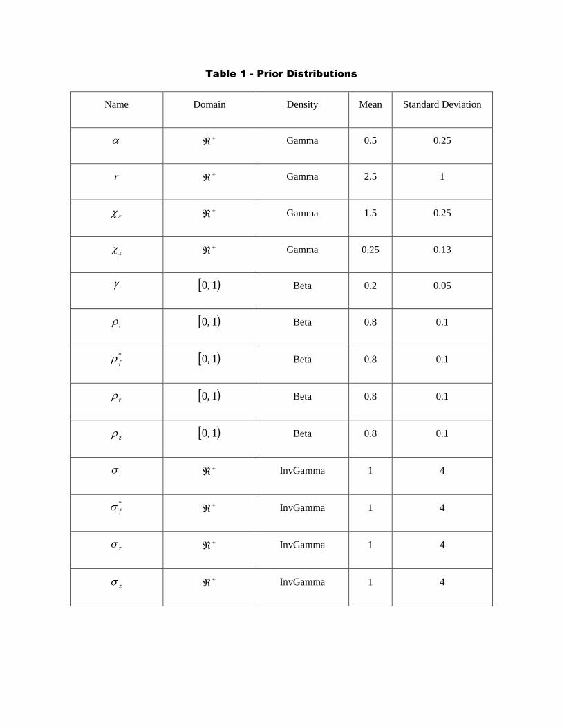
Table 1 - Prior Distributions

Name Domain Density Mean Standard Deviation

Gamma 0.5 0.25

r Gamma 2.5 1

Gamma 1.5 0.25

x Gamma 0.25 0.13

1,0 Beta 0.2 0.05

i 1,0 Beta 0.8 0.1

*

f 1,0 Beta 0.8 0.1

1,0 Beta 0.8 0.1

z 1,0 Beta 0.8 0.1

i InvGamma 1 4

*

f InvGamma 1 4

InvGamma 1 4

z InvGamma 1 4

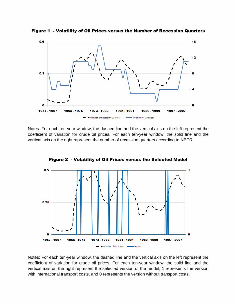
Figure 1 - Volatility of Oil Prices versus the Number of Recession Quarters

Notes: For each ten-year window, the dashed line and the vertical axis on the left represent the

coefficient of variation for crude oil prices. For each ten-year window, the solid line and the

vertical axis on the right represent the number of recession quarters according to NBER.

Figure 2 - Volatility of Oil Prices versus the Selected Model

Notes: For each ten-year window, the dashed line and the vertical axis on the left represent the

coefficient of variation for crude oil prices. For each ten-year window, the solid line and the

vertical axis on the right represent the selected version of the model; 1 represents the version

with international transport costs, and 0 represents the version without transport costs.

Figure 3 - Variance Decomposition of U.S. GDP with Transport Costs

1960-1970 1970-1980 1980-1990 1990-2000 2000-2010

0

20

40

60

80

100

Foreign Financial

Monetary Policy

Technology

Transport Costs

Notes: For each ten-year window, the colored areas show the HP filtered (=1600) contribution

of the relevant shocks on the volatility of U.S. GDP.

Figure 4 - Variance Decomposition of U.S. GDP without Transport Costs

1960-1970 1970-1980 1980-1990 1990-2000 2000-2010

0

20

40

60

80

100

Foreign Financial

Monetary Policy

Technology



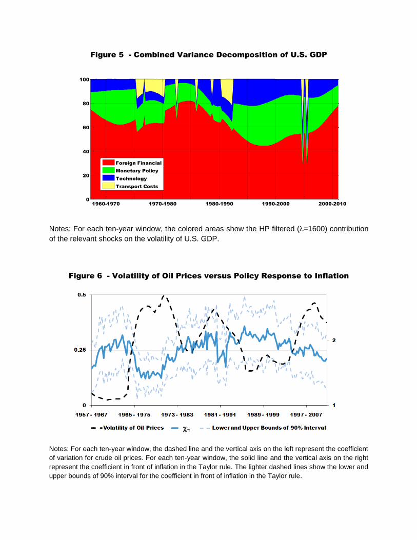
Figure 5 - Combined Variance Decomposition of U.S. GDP

1960-1970 1970-1980 1980-1990 1990-2000 2000-2010

0

20

40

60

80

100

Foreign Financial

Monetary Policy

Technology

Transport Costs



Figure 6 - Volatility of Oil Prices versus Policy Response to Inflation

Notes: For each ten-year window, the dashed line and the vertical axis on the left represent the coefficient

of variation for crude oil prices. For each ten-year window, the solid line and the vertical axis on the right

represent the coefficient in front of inflation in the Taylor rule. The lighter dashed lines show the lower and

upper bounds of 90% interval for the coefficient in front of inflation in the Taylor rule.

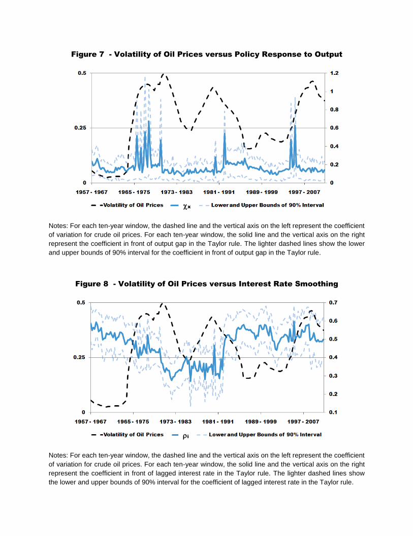
Figure 7 - Volatility of Oil Prices versus Policy Response to Output



represent the coefficient in front of output gap in the Taylor rule. The lighter dashed lines show the lower

and upper bounds of 90% interval for the coefficient in front of output gap in the Taylor rule.

Figure 8 - Volatility of Oil Prices versus Interest Rate Smoothing



represent the coefficient in front of lagged interest rate in the Taylor rule. The lighter dashed lines show

the lower and upper bounds of 90% interval for the coefficient of lagged interest rate in the Taylor rule.

x

i

Documents

Oil Shocks through International Transport Costs: Evidence