Embed Size (px)
Citation preview

TS06J - Hydrography and the Environment
Olusegun Badejo and Peter Nwilo
Oil Spill Model for Oil Pollution Control
FIG Working Week 2011
Bridging the Gap between Cultures
Marrakech, Morocco, 18-22 May 2011
1/29
Oil Spill Model for Oil Pollution Control
Olusegun BADEJO and Peter NWILO, Nigeria
Key words: Oil Spill, Model
SUMMARY
Few studies have been carried out on oil spill trajectory and fate modeling. Limited modeling
and observation suggest that oil spill move as the bulk water moves and that the water moves
in concert with mass circulation including the influence of currents and tides. Additional
influences in the movement of oil spill include vertical mixing and sedimentation.
A new oil spill trajectory model has been developed in this work. The relationship and the
effect of waves induced current in the transport of oil spill on water was considered in the
development of the model. Appropriate wave driven current equation was coupled with that
of wind drift current, ocean current, tidal current and longshore current equations to generate
a new model for advecting oil spill on coastal waters. Relevant equations for calculating the
rate of spreading and evaporation of oil were also included in the oil spill model to enable the
determination of the fate of oil spill.
A hypothetical spill site around OPL 250 located about 150km off the Nigerian coastline and
another site located around Idoho, about 25km from Nigerian coastline were used as study
areas for this work. Oil spill simulations with the new model were made for wet and dry
seasons for these study areas.
Results from the new model indicate that for both wet and dry seasons, the ocean current is
the major factor for moving the oil spill from the Atlantic Ocean to fairly deep waters. While
the Longshore current and tides are the dominant forces that move the oil spill in shallow
waters. Wind drift current and wave drift currents are secondary factors for moving the oil spill
during wet and dry seasons.
Statistical analysis using Hotelling’s T2 indicates that the effect of adding waves parameters does
not significantly affect the oil spill result. However, the accuracy of the oil spill model is
improved by adding the wave parameters. Results from this work show that the incorporation of
wave parameters into the oil spill model causes the oil spill to get to the shore a few hours earlier
than when the wave parameters were neglected in the model.
There is a need for a better understanding of the coastal ecology so as to evaluate the
significance of the impacts generated by oil spill incidents. The Federal Government in
conjunction with oil parastatals and other non-governmental agencies should create more
meteorological stations near the shoreline or on the coastal waters. The meteorological stations
should provide real time or predicted meteorological data of the surrounding environment. This
data would serve among other things as input data into oil spill models.

TS06J - Hydrography and the Environment
Olusegun Badejo and Peter Nwilo
Oil Spill Model for Oil Pollution Control
FIG Working Week 2011
Bridging the Gap between Cultures
Marrakech, Morocco, 18-22 May 2011
2/29
Oil Spill Model for Oil Pollution Control
Olusegun BADEJO and Peter NWILO, Nigeria
1. INTRODUCTION
Oil releases have increasingly become a concern in recent years. Integrated oil/chemical fate
and impact model systems may be used to quantify environmental impacts and damages
resulting from real events, hypothetical spills (ecological risk assessment), and various
response strategies (contingency planning), such that objective decision-making may occur
(French McCay, 2006).
Studies on oil spill have shown that physical, chemical, and biological processes that depend
on oil properties, hydrodynamics, and meteorological and environmental conditions govern
the transport and fate of spilled oil in water bodies. These processes include advection,
turbulent diffusion, surface spreading, evaporation, dissolution, emulsification, hydrolysis,
photo-oxidation, biodegradation and particulation.
Few studies have been conducted on the subsurface advection of oil (Spaulding, 1995).
Limited modeling and observation suggest that the dissolved and particulate oil move as the
bulk water moves and that the water moves in concert with mass circulation including the
influence of currents and tides (Spaulding, 1995). Additional influences in the subsurface
movement include vertical mixing by Langmuir circulation (McWilliams and Sullivan, 2000).
The model due to Fay (1969, 1971) for oil spill spreading model is generally used by oil spill
analysts to model oil spill dispersion. Dispersion is also modeled using a Fickian law that
assumes a neutrally buoyant, noncohesive substance. Some composite oil slick models simply
ignore horizontal dispersion and focus on the “center of mass” of the slicks. The National
Oceanic and Atmospheric Administration’s GNOME model uses a Fickian law. Others have
developed heuristic methods with coefficients tuned to observed slick data. Examples include
Morales et al. (1997) who have developed a random-walk method and Howlett et al. (1993)
who break the spill into parcels called “spillets” and disperse them numerically.
Vertical dispersion and entrainment are the movements of oil droplets of sizes less than about
100 μm into the water column. MacKay developed an early model of entrainment based on
the square of wind speed, the viscosity of oil, slick thickness, and surface tension (Reed 1992;
ASCE, 1996). Tests of this model showed that it provided reasonable results at moderate wind
speeds, but otherwise deviated from experimental values. Delvigne et al. (1987) and Delvigne
(1993) developed a series of models based on a number of different flume tests, tank tests,
and at-sea measurements.
Sinking is the mechanism by which oil masses that are denser than the receiving water are
transported to the bottom. The oil itself may be denser than water, or it may have incorporated
enough sediment to become denser than water. Sedimentation is the sorption of oil to

TS06J - Hydrography and the Environment
Olusegun Badejo and Peter Nwilo
Oil Spill Model for Oil Pollution Control
FIG Working Week 2011
Bridging the Gap between Cultures
Marrakech, Morocco, 18-22 May 2011
3/29
suspended sediments that eventually settle out of the water column and accumulate on the
seafloor. There is a significant difference in the relative amount of oil incorporated by the two
processes; sinking oil may contain a few percent sediment, whereas contaminated sediments
accumulating on the seafloor will contain at most a few percent oil (McCourt and Shier,
2001).
Initial prediction of oil evaporation was carried out by using water evaporation equations such
as the one developed by Sutton (1934). Later work of Mackay and colleagues (Mackay and
Matsugu, 1973; Stiver and Mackay, 1984) was applied to describe the evaporation of crude
oil through the use of mass-transfer coefficients as a function of wind speed and spill area.
Stiver and Mackay (1984) further developed relationships between evaporative molar flux,
mass transfer coefficient at prevailing wind speed, area of spill, vapor pressure of the bulk
liquid, gas constant, and temperature.
Advection and spreading have been identified as the major factors responsible for moving oil
spill on water by these models (Egberongbe et al, 2006). In many oil spills, evaporation is the
most important process in terms of mass balance. Within a few days following a spill, light
crude oils can lose up to 75 percent of their initial volume and medium crudes up to 40
percent. In contrast, heavy or residual oils will lose not more than 10 percent of their volume
in the first few days following a spill. Most oil spill behavior models include evaporation as a
process and as a factor in the output of the model (National Academy of Sciences, 2003).
Oil dissolution, emulsification, biodegradation, photosynthesis and sedimentation are minor
factors affecting oil spill and are negligible because they are slow and gradual processes. They
are however important in knowing the fate of oil spill over a long period of time.
Wind drift current, ocean current and tides are used by oil models for advecting oil spill on
water. A fixed percentage (3-4%) of the speed of wind is assumed for the wind drift current.
The bearing of the wind plus a deflection angle is taken as the bearing of the wind drift
current. One hundred to one hundred and ten percent of the speed of real time ocean current
or assumed ocean current from historic ocean current data are used in the models. The bearing
of the ocean current is also obtained in real time or from historic data. Some of the oil models
obtained their tidal information from existing tidal or hydrodynamic models, while others
neglect the effect of tides in their models. Wind drift speed and bearing, ocean current speed
and bearing, and tidal speed and bearing are vector summed in oil spill models to get the
speed and bearing of oil spill on water.
2. DEVELOPMENT OF A NEW MODEL FOR OIL POLLUTION CONTROL
Despite the fact that many oil spill models have been developed, most of the existing models
have not been able to accurately track the movement of oil spill on coastal waters. The
reasons for this are that many assumptions have been made in the development of these
models. While some of the models assume a certain percentage of wind velocity as the oil
drift factor, some ignore other factors that move oil spill on water. Furthermore ignorance of
TS06J - Hydrography and the Environment
Olusegun Badejo and Peter Nwilo
Oil Spill Model for Oil Pollution Control
FIG Working Week 2011
Bridging the Gap between Cultures
Marrakech, Morocco, 18-22 May 2011
4/29
the physical and meteorological characteristics of the surrounding water bodies has led to the
failure of the deployment of these models.
In this work a new model has been developed. In the development of this model, emphasis is
laid on identification of all major factors that govern the movement of oil on water. We have
also used theoretical mathematical equations that govern these major factors to develop the
new oil spill model. The following is the thereotical framework that was used to develop the
model:
1. Two Dimensional Hyperbolic Wind Drift Equation Based on Newton’s Law.
2. Airy’s Eulerian Wave Theory with Taylor’s Series Expansion.
3. Tidal Current Analysis by Dean and Dalrymple.
4. Fay’s Spreading Laws.
5. MacKay’s Evaporative Formula.
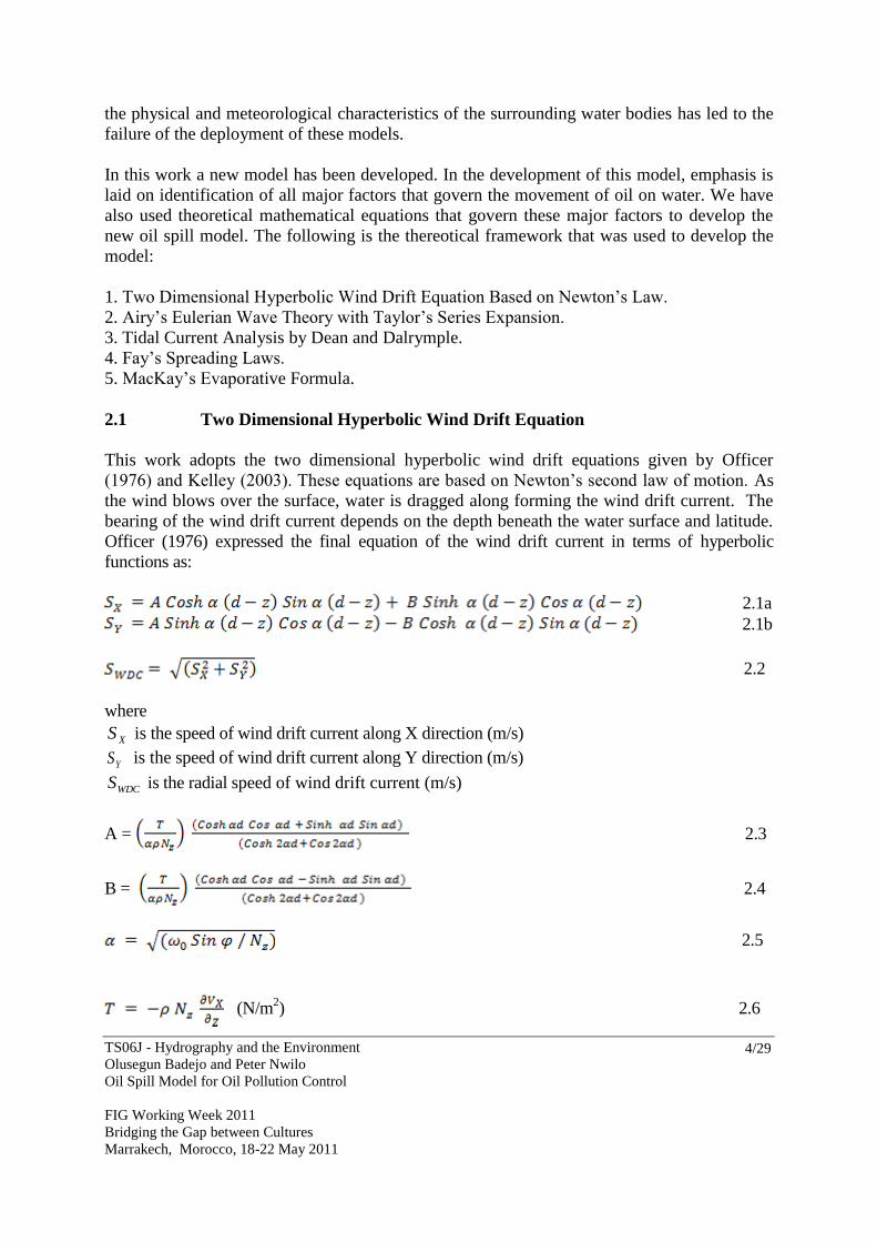
2.1 Two Dimensional Hyperbolic Wind Drift Equation
This work adopts the two dimensional hyperbolic wind drift equations given by Officer
(1976) and Kelley (2003). These equations are based on Newton’s second law of motion. As
the wind blows over the surface, water is dragged along forming the wind drift current. The
bearing of the wind drift current depends on the depth beneath the water surface and latitude.
Officer (1976) expressed the final equation of the wind drift current in terms of hyperbolic
functions as:
2.1a
2.1b
2.2
where
XS is the speed of wind drift current along X direction (m/s)
YS is the speed of wind drift current along Y direction (m/s)
WDCS is the radial speed of wind drift current (m/s)
A = 2.3
B = 2.4
2.5
(N/m2) 2.6

TS06J - Hydrography and the Environment
Olusegun Badejo and Peter Nwilo
Oil Spill Model for Oil Pollution Control
FIG Working Week 2011
Bridging the Gap between Cultures
Marrakech, Morocco, 18-22 May 2011
5/29
z is the depth of liquid measured positively downwards ( z = 0 on water surface).
d is the bottom depth (m).
is the density of sea water (kg/m3)
is the rate of change of the speed of the wind drift in the X direction with respect to depth
v = Coefficient of kinematic viscosity of fluid (m2/s)
0 = Angular velocity of earth’s rotation = (rad/s)
T1 = Period of the earth’s rotation = 0.0000729 rad/s.
Due to the difficulty in determinining in equation 2.6, Kelley (2003) gave the following
formular for the tangential wind stress (T): 2UCT da
(N/m2) 2.7
where
a = Air Density (kg/m3)
dC = Drag Coefficient (0.001 for calm sea, 0.002 for rough sea)
U= Wind Speed (m/s)
Buranapratheprat and Tanjaaitrong (2000) stated that the deflection angle of the wind drift
current depends on latitude. For latitudes between 100 N and 10
0 S, the deflection angle ()
reduces linearly with latitude and can be approximated as:
)10/(33 O 2.8
The wind drift bearing is therefore the sum of the wind bearing and the deflection angle
expressed as:
WDC Wind bearing+ )10/(33 O 2.9
where
WDC Wind Drift bearing (o)
2.2 Airy’s Eulerian Wave Theory with Taylor’s Series Expansion
The Eulerian wave drift current in this work is based on Airy’s wave theory with a Taylor’s
series expansion given by Sobey and Barker (1997). The wave drift current equations depend on
wave speed, wave frequency, wave period and wave number. The wave number is determined by
dispersion relation given by Lamb (1932) and solved using Newton Raphson’s iteration method.
The wave averaged Eulerian surface drift is:
CkaSSWD
2)(5.0 2.10
where

TS06J - Hydrography and the Environment
Olusegun Badejo and Peter Nwilo
Oil Spill Model for Oil Pollution Control
FIG Working Week 2011
Bridging the Gap between Cultures
Marrakech, Morocco, 18-22 May 2011
6/29
SWDS = Speed of surface wave drift (m/s)
k = Wave number (cm-1
)
a = Wave amplitude (m)
C = Wave speed (m/s)
Wave Speed (C) = Wave frequency/Wave number
Wave frequency ( ) =
Tw = Wave period (s)
Wave number (k) can be determined by the following dispersion relation given by Lamb (1932):
)tanh(2 kdgk 2.11
where
= Wave frequency (Hz)
g = Force of gravity (m/s2)
k = Wave number (cm-1
)
d = Water depth (m)
The dispersion equation in equation 2.11 above can only be solved iteratively. Newton
Raphson’s iteration method given in equation 2.12a was used to solve the dispersion equation:
)(/)( '
1 kFkFkk nn 2.12a
where
))((/)(' kFdkdkF
)))tanh()(sec/()tanh((( 22
1 kdgkdhgkdkdgkkk nn 2.12b
)/()()tanh( kdkdkdkd eeeekd 2.13
Initial approximation for k given below can be determined from shallow water
approximation where kdkd )tanh( . Substituting (kd) for tanh(kd) gives:
dgk22
)/( 2 gdk 2.14
Initial approximation for k can also be determined from deep water approximation
where tanh (kd) = 1
2.15
= Wave frequency (Hz)
SWD = direction of the Eulerian surface wave drift (the same as that of the wind).
2.3 Tidal Current Analysis
The tidal equation for determining horizontal speed of tide in this work is based on tidal
current analysis by Dean and Dalrymple (1984). The tidal current analysis is a function of the
amplitude of the tide, the wave frequency, wave number, water depth, distance and time. The
tidal currents experienced along the Nigerian Coast are semi-diurnal tides with a period of

TS06J - Hydrography and the Environment
Olusegun Badejo and Peter Nwilo
Oil Spill Model for Oil Pollution Control
FIG Working Week 2011
Bridging the Gap between Cultures
Marrakech, Morocco, 18-22 May 2011
7/29
approximately 25hours (Nwilo, 1995). Tides are significant in moving oil along the creeks.
During the floods the oil spill moves upstream, and at times of ebbs, the water and oil spill
recede.
The horizontal speed of a particle of tide along the wave direction from origin is given by
Dean and Dalrymple (1984) as:
)()(
))((tkxCos
khSinh
zhkCoshaSTIDE
2.16
For shallow waters and at water surface, the horizontal speed of a particle of tide becomes
)( tkxCosaSTIDE 2.17
= Wave frequency 2.18
T is wave period
h is water depth (m)
a is Amplitude of tide (Half tidal range (m))
t is time (0-25 hour)
k is wave number (given in section 2.2)
x is distance (m)
The assumption made here is that the heights of the two high waters and the two low waters in
a day are the same and that they have a regular period of 12.5hours. The average of the two
high waters and the two low waters predicted by Nigerian Navy tide tables is used to compute
the amplitude of the tide for a given area. This amplitude together with the phase angle of the
tide will be used to predict the speed of the tidal current. The times of high and low waters in
a day will be related to the times of crests and troughs of our tidal curve. Figure 2.1 shows a
tidal current curve with amplitude 0.44m and phase difference of 1040. The high waters will
occur at 3.125hr and 15.625hr while the low waters will occur at 9.375hr and 21.875hr. The
periods of high waters and low waters are always the same on the assumed tidal current curve
for any combination of amplitude and phase difference for a tide with a period of 12.5hrs. The
time of the tide on our assumed tidal current curve is related to the actual time of tide by the
relationship equation below:
t = 3.125 + (tactual – THW) 2.19
where
t = Time of tide on our assumed tidal curve
tactual = Actual time of the day (0-24hr)
THW = Time of high water.
Thus for any given time tactual, the corresponding time t on our assumed tidal curve can be
calculated by equation 2.19 while the speed of the tide would be calculated by equation 2.17.
The bearing of tide ( TIDE ) for a progressive tide is the wind or wave bearing during floods and
opposite the wind or wave bearing during ebbs (Canadian hydrographic service, 2005).
TIDE = Wind Bearing O180 2.20

TS06J - Hydrography and the Environment
Olusegun Badejo and Peter Nwilo
Oil Spill Model for Oil Pollution Control
FIG Working Week 2011
Bridging the Gap between Cultures
Marrakech, Morocco, 18-22 May 2011
8/29
2.4 Fay’s Spreading Laws
Fay’s spreading theory of 1971 was used in this work. In Fay’s theory oil spill is considered
to pass through three phases. In the first phase, only gravity and inertial forces are important.
In the second phase, the gravity and viscous forces dominate. The balance between surface
tension and viscous forces governs the last phase. To apply this theory, the geometry for the
oil slick is simplified into either one-dimensional or radial form. The criterion to determine
the geometry of the oil slick is through the calculation of the aspect ratio. When the aspect
ratio is less than 3, the radial spreading will be used. Formulas for spreading laws and rates of
these two forms are given by (Reddy and Brunet, 1997). Table 2.1 shows Fay’s spreading
laws.
Table 2.1: Spreading Law for Oil Slicks
Spreading Phase One Dimensional Spreading
Width (m)
Axi Symmetrical
Spreading Radius R (m)
Gravity-Inertia 3/12 )(39.1 gAt 4/12 )(14.1 gVt
Gravity-Viscous 4/12/12/32 )(39.1 vtgA 6/12/12/32 )(98.0 vtgV
Surface Tension
Viscous
4/11232 )(43.1 v
wt 4/11232 )(60.1 v
wt
Figure 2.1: Tidal Current Curve
TS06J - Hydrography and the Environment
Olusegun Badejo and Peter Nwilo
Oil Spill Model for Oil Pollution Control
FIG Working Week 2011
Bridging the Gap between Cultures
Marrakech, Morocco, 18-22 May 2011
9/29
where
V = Volume of oil slick (m
3)
v = kinematic viscosity (m2/s)
t = time (s)
g = force of gravity (m/s2)
w = Density of water (g/cm3)
A = Spill area (m2)
Density of oil (g/cm3)
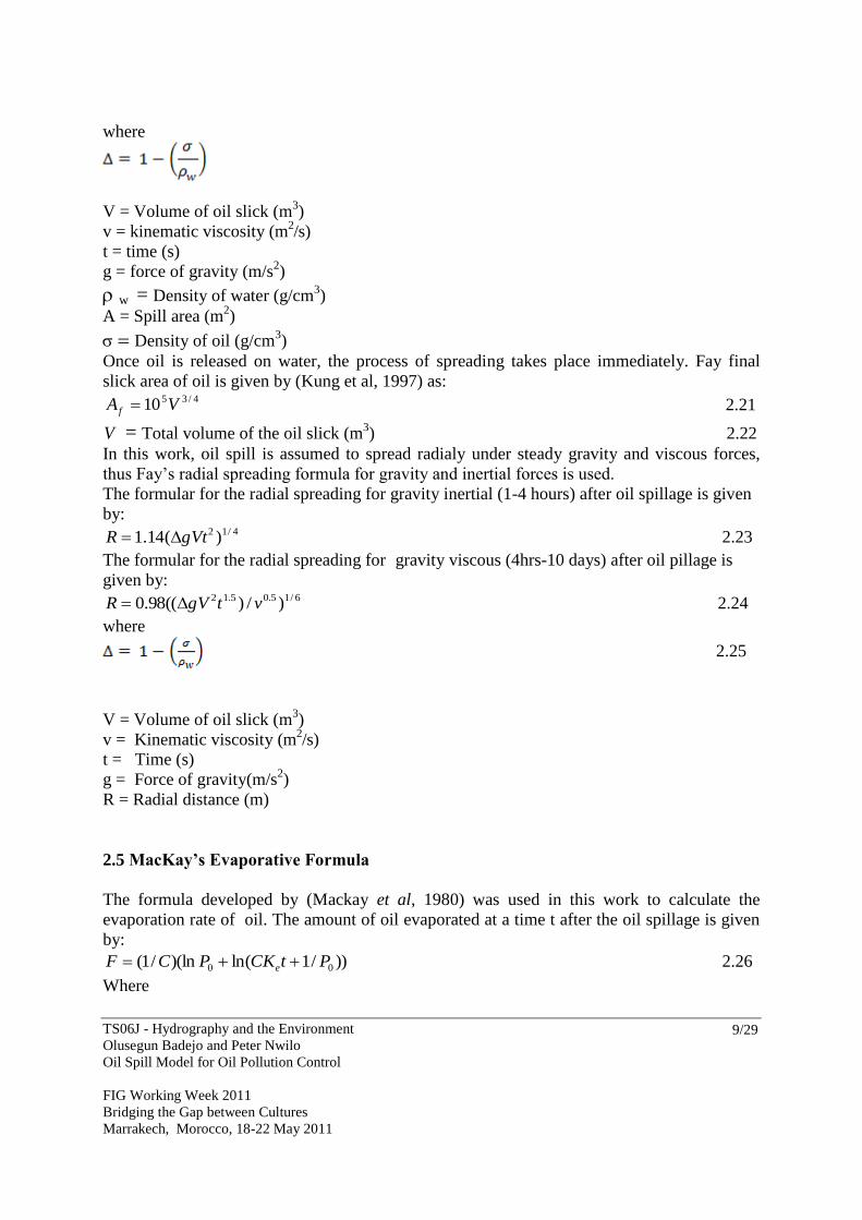
Once oil is released on water, the process of spreading takes place immediately. Fay final
slick area of oil is given by (Kung et al, 1997) as: 4/3510 VA f 2.21
V = Total volume of the oil slick (m3) 2.22
In this work, oil spill is assumed to spread radialy under steady gravity and viscous forces,
thus Fay’s radial spreading formula for gravity and inertial forces is used.
The formular for the radial spreading for gravity inertial (1-4 hours) after oil spillage is given
by: 4/12 )(14.1 gVtR 2.23
The formular for the radial spreading for gravity viscous (4hrs-10 days) after oil pillage is
given by: 6/15.05.12 )/)((98.0 vtgVR 2.24
where
2.25
V = Volume of oil slick (m3)
v = Kinematic viscosity (m2/s)
t = Time (s)
g = Force of gravity(m/s2)
R = Radial distance (m)
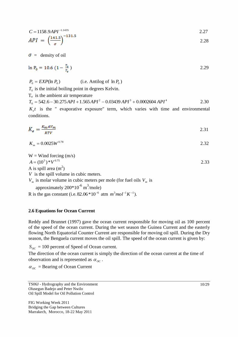
2.5 MacKay’s Evaporative Formula
The formula developed by (Mackay et al, 1980) was used in this work to calculate the
evaporation rate of oil. The amount of oil evaporated at a time t after the oil spillage is given
by:
))/1ln()(ln/1( 00 PtCKPCF e 2.26
Where
TS06J - Hydrography and the Environment
Olusegun Badejo and Peter Nwilo
Oil Spill Model for Oil Pollution Control
FIG Working Week 2011
Bridging the Gap between Cultures
Marrakech, Morocco, 18-22 May 2011
10/29
1435.19.1158 APIC 2.27
2.28
= density of oil
) 2.29
)(ln 00 PEXPP (i.e. Antilog of 0ln P )
0T is the initial boiling point in degrees Kelvin.
Te is the ambient air temperature 432
0 0002604.003439.0565.1275.306.542 APIAPIAPIAPIT 2.30
tKe is the " evaporative exposure" term, which varies with time and environmental
conditions.
2.31
78.00025.0 WKm 2.32
W = Wind forcing (m/s) 75.05 *)10( VA 2.33
A is spill area (m2)
V is the spill volume in cubic meters.
mV is molar volume in cubic meters per mole (for fuel oils mV is
approximately 200*10-6
m3/mole)
R is the gas constant (i.e. 610*06.82 atm 113 Kmolm ).
2.6 Equations for Ocean Current
Reddy and Brunnet (1997) gave the ocean current responsible for moving oil as 100 percent
of the speed of the ocean current. During the wet season the Guinea Current and the easterly
flowing North Equatorial Counter Current are responsible for moving oil spill. During the Dry
season, the Benguela current moves the oil spill. The speed of the ocean current is given by:
OCS = 100 percent of Speed of Ocean current.
The direction of the ocean current is simply the direction of the ocean current at the time of
observation and is represented as OC .
OC = Bearing of Ocean Current

TS06J - Hydrography and the Environment
Olusegun Badejo and Peter Nwilo
Oil Spill Model for Oil Pollution Control
FIG Working Week 2011
Bridging the Gap between Cultures
Marrakech, Morocco, 18-22 May 2011
11/29
2.7 Model for Longshore Current
Although waves tend to become parallel with the coast as a result of refraction, they usually
break at a slight angle to the shore, with the result that a littoral or longshore current is
induced and is effective in moving a mass of water slowly along the coast. Longshore drift is
the prevalent sediment transport mechanism along the Nigerian coastline and is basically
within the first 5km kilometres offshore. The whole magnitude of the speed of the longshore
current is responsible for moving oil spill along the coastline. The oil spill will also move in the
direction or bearing of the longshore current. The speed and direction of the Longshore current is
represented as LCS and LC respectively in this work.
LCS = Speed of Longshore Current
LC = Bearing of Longshore Current
2.8 Final Equations of the Oil Spill Model
An integrated dynamic oil spill trajectory model for advecting oil spill on open- water was
evolved after finding the resultant of the equations for the wind drift current speed and
bearing, the Eulerian surface wave drift speed and bearing, tidal speed and bearing, ocean
current speed and bearing and longshore current speed and bearing (Egberongbe et al, 2006).
The resultant of the equations (speed of oil spill) is given by:
2)(( LCLCOCOCTIDETIDESWDSWDWDCWDCNM SinSSinSSinSSinSSinSS 2/12 ))( LCLCOCOCTIDETIDESWDSWDWDCWDC CosSCosSCosSCosSCosS 2.34
The angle between the resultant and the x-axis is given by:
2.35
where
SNM = Speed of oil spill on open water
αNM = Bearing of oilspill on open water
SWDC = Speed of wind drift current.
WDC = Bearing of wind drift current.
SSWD = Speed of Eulerian surface wave drift current.
SWD = Bearing of Eulerian surface wave drift current.
STIDE = Speed of tide.
TIDE = Bearing of tide.
SOC = Speed of ocean current.
OC = Bearing of ocean current.
TS06J - Hydrography and the Environment
Olusegun Badejo and Peter Nwilo
Oil Spill Model for Oil Pollution Control
FIG Working Week 2011
Bridging the Gap between Cultures
Marrakech, Morocco, 18-22 May 2011
12/29
SLC = Speed of longshore current
LC = Bearing of longshore current
The equations for SWDC, WDC, SSWD, SWD, STIDE, TIDE, are given in equations 2.2, 2.9, 2.10,
2.15, 2.17 and 2.20 respectively, while SOC, OC, SLC and LC are explained in sections 2.6
and 2.7.
The model equations for spreading are given by equations 2.21, 2.23 and 2.24. Equation 2.26
is the model equation for evaporation.
2.9 Study Areas and Model Implementation
Two study areas were used in this work. A hypothetical spill site around OPL 250 located
about 150km off the Nigerian coastline was chosen as study area I (Nwilo and Badejo, 2006).
The actual spill position is longitude 4o 30’ 46.20” E and latitude 4
o 25’ 39.80” N. Simulations
were made for wet and dry seasons for study area I. Study area II is located around Idoho,
about 25km from Akwa Ibom State coastline. The oil spill point is Longitude 8o 00’, Latitude 4
o
20’N. Simulations were also made for wet and dry seasons for study area II.
The OILMAP model was also used to make simulations for the same study area above for wet
and dry seasons.
3. RESULTS AND ANALYSIS OF RESULTS
The sections in this chapter contain the results of oil spill simulation with the model developed in
this work and the results of other models. Hypotheses testing and analysis of the results were
also carried out in this chapter.
3.1 Results
The following sub sections contain the oil spill trajectory model’s results for oil spill simulation
in study area I and study area II for both wet and dry seasons
3.1.1 Results of Oil Spill Simulation with the New Model for Study Area I (Wet Season)
The summary of the results in wet season is given in Table 3.1. The simulated oil spill points
for all the phases for the wet season were plotted in ArcGIS software, which is linked with the
model in ArcGIS Visual Basic environment. The Oil Spill Trajectory for the wet season in
Study Area I is shown in Figure 3.1. The result for wet season for the study area indicate that
the simulated oil spill will reach the shore line between Kulama River and Penington River after
122hours (5days), and then move towards Ramos river along the direction of the longshore
current. The oil spill will move inlands during high tides and back to its position along the
shoreline when the tides are low. The oil spill will reach Ramos River in 150 hours.

TS06J - Hydrography and the Environment
Olusegun Badejo and Peter Nwilo
Oil Spill Model for Oil Pollution Control
FIG Working Week 2011
Bridging the Gap between Cultures
Marrakech, Morocco, 18-22 May 2011
13/29
Table 3.1: Summary of Results of New Oil Spill Model for Study Area I During
the Wet Season
Very Deep
Waters (500m)
Deep Waters
(50m)
Fairly Deep Waters
(15m)
Shallow Waters
(5m)
Oil Spill Speed 0.294m/s 0.285-0.304 m/s 0.178-0.476m/s 0.584-0.713m/s
Oil Spill Bearing 83.09- 83.10 deg 81.59- 84.58deg 66.99 –135.12deg 311.69 – 349.67deg
Ocean Current
Speed
0.233m/s 0.233m/s 0.233m/s -
Ocean Current
Bearing
90o (East) 90
o (East) 90
o (East) -
Wind Drift Speed 0.065m/s 0.065m/s 0.051m/s 0.018m/s
Wind Drift
Bearing
59.61 deg 59.90deg 59.99deg 60.04deg
Wave Drift Speed 0.003m/s 0.004m/s 0.006m/s 0.011m/s
Wave Drift
Bearing
45 deg 45deg 45deg 45deg
Tidal Speed - 0 – 0.013 m/s 0-0.22m/s 0-0.22m/s
Tidal Bearing - 45/225 45/225deg 45/225deg
Longshore
Current Speed
- - - 0.61m/s
Figure 3.1: Oil Spill Trajectory for Wet Season in Study Area I

TS06J - Hydrography and the Environment
Olusegun Badejo and Peter Nwilo
Oil Spill Model for Oil Pollution Control
FIG Working Week 2011
Bridging the Gap between Cultures
Marrakech, Morocco, 18-22 May 2011
14/29
Longshore
Current Bearing
- - - 330 deg
3.1.2 Results of Oil Spill Simulation with the New Model for Study Area I (Dry Season)
The summary of the results in dry season is given in Table 3.2. The simulated oil spill points for
all the phases for the dry season in study area I were plotted in ArcGIS environment, which is
linked with the oil spill trajectory model in Visual Basic environment and shown in Figure 3.2.
The result for the dry season for the study area indicates that the simulated oil spill will reach the
shore in 213 hours and get to Benin River after 222 hours (nine days). The oil spill will pollute
Benin River and it’s adjoining areas. The oil spill will move inlands during high tides and back
to its position along the shoreline when the tides are low.
Table 3.2: Summary of Results of New Oil Spill Model for Study Area I During
the Dry Season Very Deep
Waters (500m)
Deep Waters
(50m)
Fairly Deep Waters
(15m)
Shallow Waters
(5m)
Oil Spill Speed 0.221-0.222m/s 0.207-0.231 m/s 0.101 – 0.416m/s 0.398 – 0.460m/s
Oil Spill Bearing 17.80- 18.12 deg 16.99 – 20.00 deg 294.47 – 30.95deg 104.72 – 160.016deg
Figure 3.2: Oil Spill Trajectory for Dry Season in Study Area I

TS06J - Hydrography and the Environment
Olusegun Badejo and Peter Nwilo
Oil Spill Model for Oil Pollution Control
FIG Working Week 2011
Bridging the Gap between Cultures
Marrakech, Morocco, 18-22 May 2011
15/29
Ocean Current
Speed
0.17m/s 0.17m/s 0.17m/s -
Ocean Current
Bearing
0o (North) 0
o (North) 0
o (North) -
Wind Drift Speed 0.076-0.077m/s 0.075-0.076m/s 0.060m/s 0.022m/s
Wind Drift
Bearing
59.61 deg 62.56deg 63.63deg 64.35deg
Wave Drift Speed 0.003m/s 0.004m/s 0.006m/s 0.011m/s
Wave Drift
Bearing
45 deg 45deg 45deg 45deg
Tidal Speed - 0 – 0.013 m/s 0-0.221m/s 0.028 - 0.217m/s
Tidal Bearing - 45/225 45/225deg 45/225deg
Longshore
Current Speed
- - - 0.390m/s
Longshore
Current Bearing
- - - 135 deg
3.1.3 Results of Oil Spill Simulation with the New Model for Study Area II (Wet Season)
The results of the oil spill simulation with the new model for Study Area II is given in Table 3.3.
The simulated oil spill points for all the three phases for the wet season in study area II were
plotted in ArcGIS software which is linked with the model in ArcGIS Visual Basic environment.
The Oil Spill Trajectory for the wet season is shown in Figure 3.3.
Figure 3.3: Oil Spill Trajectory for Study Area II During the Wet Season
TS06J - Hydrography and the Environment
Olusegun Badejo and Peter Nwilo
Oil Spill Model for Oil Pollution Control
FIG Working Week 2011
Bridging the Gap between Cultures
Marrakech, Morocco, 18-22 May 2011
16/29
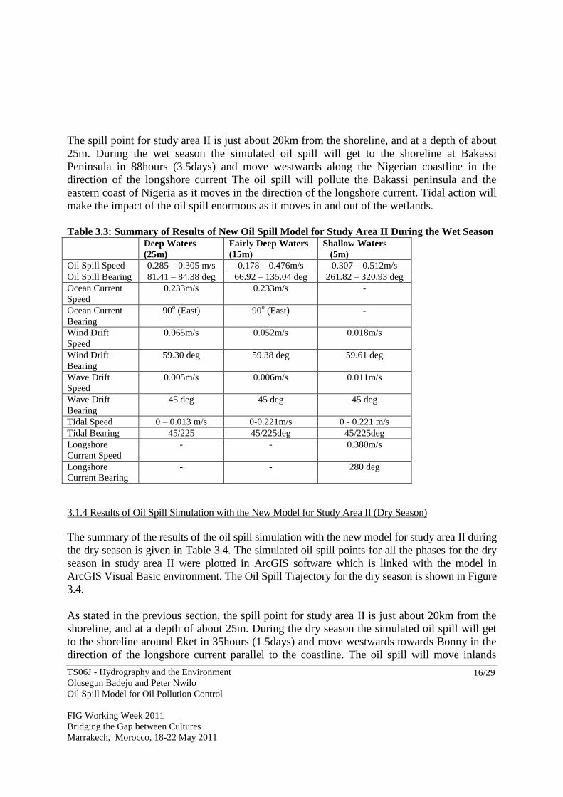
The spill point for study area II is just about 20km from the shoreline, and at a depth of about
25m. During the wet season the simulated oil spill will get to the shoreline at Bakassi
Peninsula in 88hours (3.5days) and move westwards along the Nigerian coastline in the
direction of the longshore current The oil spill will pollute the Bakassi peninsula and the
eastern coast of Nigeria as it moves in the direction of the longshore current. Tidal action will
make the impact of the oil spill enormous as it moves in and out of the wetlands.
Table 3.3: Summary of Results of New Oil Spill Model for Study Area II During the Wet Season Deep Waters
(25m)
Fairly Deep Waters
(15m)
Shallow Waters
(5m)
Oil Spill Speed 0.285 – 0.305 m/s 0.178 – 0.476m/s 0.307 – 0.512m/s
Oil Spill Bearing 81.41 – 84.38 deg 66.92 – 135.04 deg 261.82 – 320.93 deg
Ocean Current
Speed
0.233m/s 0.233m/s -
Ocean Current
Bearing
90o (East) 90
o (East) -
Wind Drift
Speed
0.065m/s 0.052m/s 0.018m/s
Wind Drift
Bearing
59.30 deg 59.38 deg 59.61 deg
Wave Drift
Speed
0.005m/s 0.006m/s 0.011m/s
Wave Drift
Bearing
45 deg 45 deg 45 deg
Tidal Speed 0 – 0.013 m/s 0-0.221m/s 0 - 0.221 m/s
Tidal Bearing 45/225 45/225deg 45/225deg
Longshore
Current Speed
- - 0.380m/s
Longshore
Current Bearing
- - 280 deg
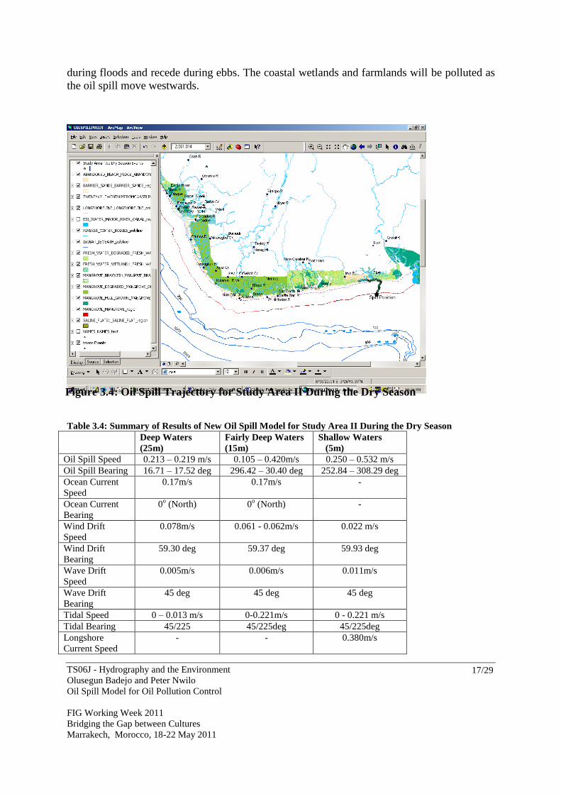
3.1.4 Results of Oil Spill Simulation with the New Model for Study Area II (Dry Season)
The summary of the results of the oil spill simulation with the new model for study area II during
the dry season is given in Table 3.4. The simulated oil spill points for all the phases for the dry
season in study area II were plotted in ArcGIS software which is linked with the model in
ArcGIS Visual Basic environment. The Oil Spill Trajectory for the dry season is shown in Figure
3.4.
As stated in the previous section, the spill point for study area II is just about 20km from the
shoreline, and at a depth of about 25m. During the dry season the simulated oil spill will get
to the shoreline around Eket in 35hours (1.5days) and move westwards towards Bonny in the
direction of the longshore current parallel to the coastline. The oil spill will move inlands
TS06J - Hydrography and the Environment
Olusegun Badejo and Peter Nwilo
Oil Spill Model for Oil Pollution Control
FIG Working Week 2011
Bridging the Gap between Cultures
Marrakech, Morocco, 18-22 May 2011
17/29
during floods and recede during ebbs. The coastal wetlands and farmlands will be polluted as
the oil spill move westwards.
Table 3.4: Summary of Results of New Oil Spill Model for Study Area II During the Dry Season
Deep Waters
(25m)
Fairly Deep Waters
(15m)
Shallow Waters
(5m)
Oil Spill Speed 0.213 – 0.219 m/s 0.105 – 0.420m/s 0.250 – 0.532 m/s
Oil Spill Bearing 16.71 – 17.52 deg 296.42 – 30.40 deg 252.84 – 308.29 deg
Ocean Current
Speed
0.17m/s 0.17m/s -
Ocean Current
Bearing
0o (North) 0
o (North) -
Wind Drift
Speed
0.078m/s 0.061 - 0.062m/s 0.022 m/s
Wind Drift
Bearing
59.30 deg 59.37 deg 59.93 deg
Wave Drift
Speed
0.005m/s 0.006m/s 0.011m/s
Wave Drift
Bearing
45 deg 45 deg 45 deg
Tidal Speed 0 – 0.013 m/s 0-0.221m/s 0 - 0.221 m/s
Tidal Bearing 45/225 45/225deg 45/225deg
Longshore
Current Speed
- - 0.380m/s
Figure 3.4: Oil Spill Trajectory for Study Area II During the Dry Season
TS06J - Hydrography and the Environment
Olusegun Badejo and Peter Nwilo
Oil Spill Model for Oil Pollution Control
FIG Working Week 2011
Bridging the Gap between Cultures
Marrakech, Morocco, 18-22 May 2011
18/29
Longshore
Current Bearing
- - 267 deg
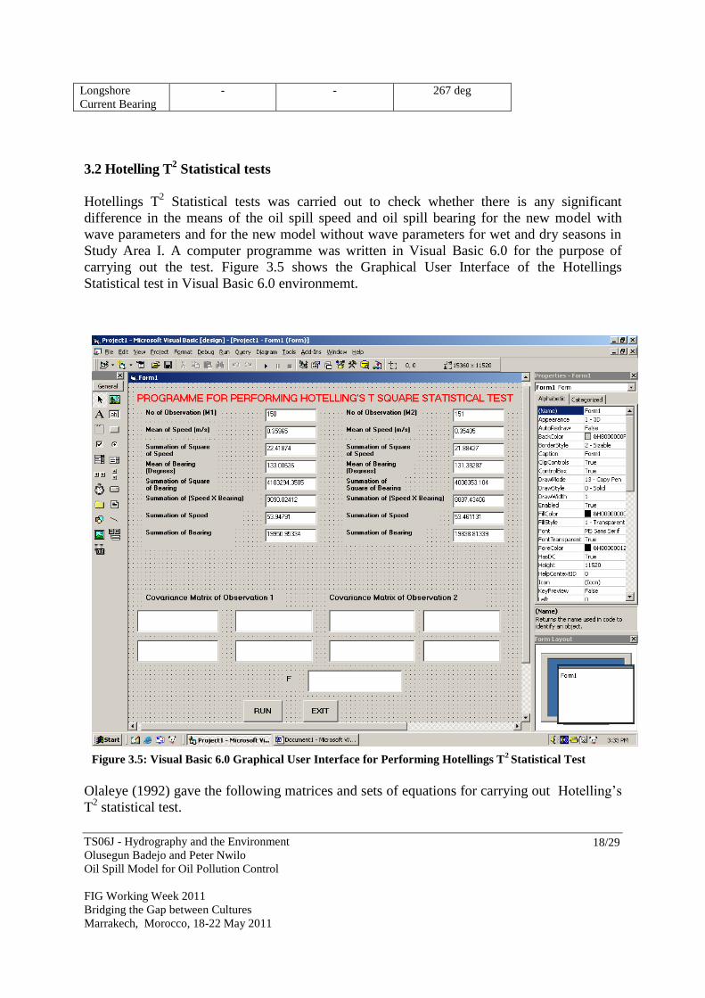
3.2 Hotelling T2 Statistical tests
Hotellings T2 Statistical tests was carried out to check whether there is any significant
difference in the means of the oil spill speed and oil spill bearing for the new model with
wave parameters and for the new model without wave parameters for wet and dry seasons in
Study Area I. A computer programme was written in Visual Basic 6.0 for the purpose of
carrying out the test. Figure 3.5 shows the Graphical User Interface of the Hotellings
Statistical test in Visual Basic 6.0 environmemt.
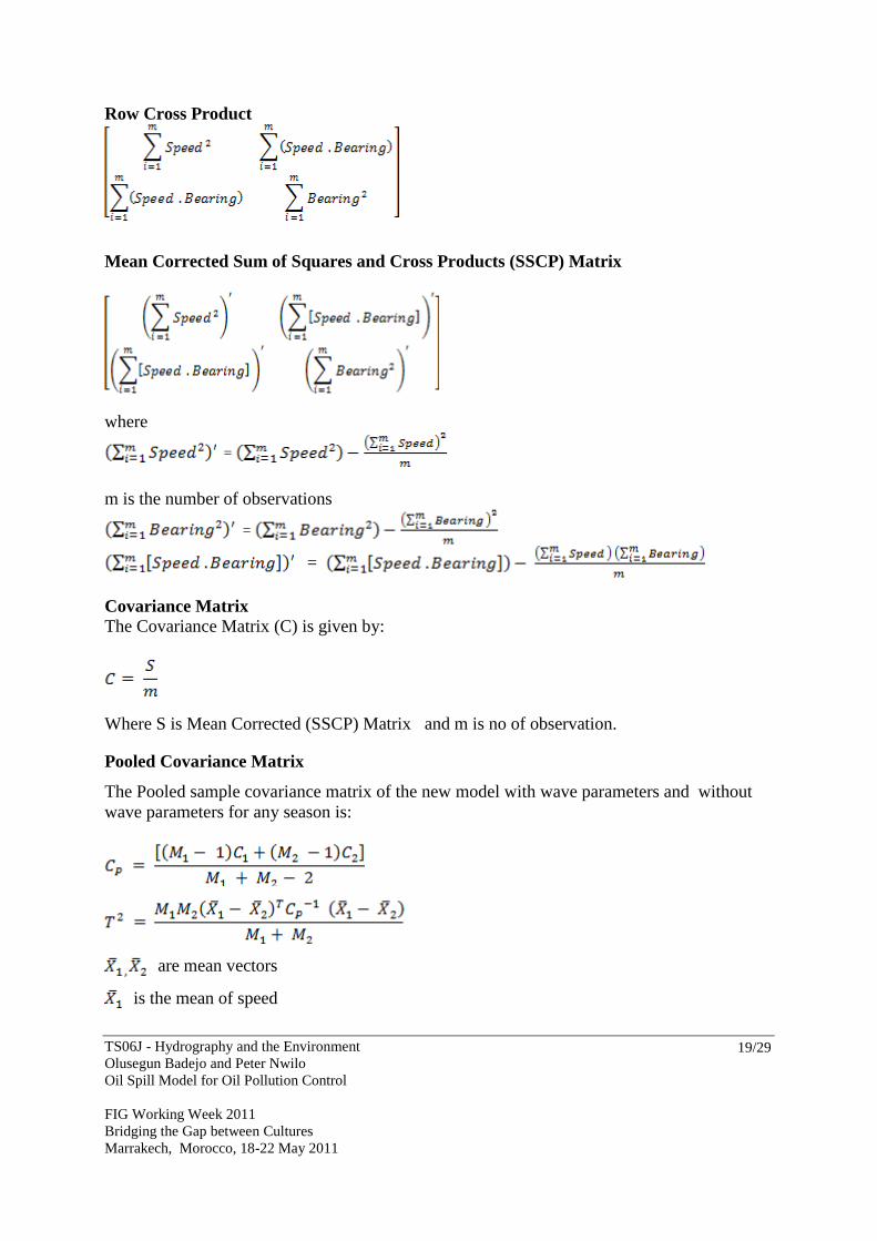
Olaleye (1992) gave the following matrices and sets of equations for carrying out Hotelling’s
T2 statistical test.
Figure 3.5: Visual Basic 6.0 Graphical User Interface for Performing Hotellings T2 Statistical Test
TS06J - Hydrography and the Environment
Olusegun Badejo and Peter Nwilo
Oil Spill Model for Oil Pollution Control
FIG Working Week 2011
Bridging the Gap between Cultures
Marrakech, Morocco, 18-22 May 2011
19/29
Row Cross Product
Mean Corrected Sum of Squares and Cross Products (SSCP) Matrix
where
=
m is the number of observations
=
=
Covariance Matrix
The Covariance Matrix (C) is given by:
Where S is Mean Corrected (SSCP) Matrix and m is no of observation.
Pooled Covariance Matrix
The Pooled sample covariance matrix of the new model with wave parameters and without
wave parameters for any season is:
are mean vectors
is the mean of speed

TS06J - Hydrography and the Environment
Olusegun Badejo and Peter Nwilo
Oil Spill Model for Oil Pollution Control
FIG Working Week 2011
Bridging the Gap between Cultures
Marrakech, Morocco, 18-22 May 2011
20/29
is the mean of bearing
M1 is the no of observations in model with wave parameters
M2 is the no of observations in model without wave parameters
Reject Ho: If F > F1- (P, M1 + M2 –P - 1)
Let α: = 0.05
For both the wet and dry seasons, F < F1-α, we therefore accepted HO that is there were no
significant differences between the results of the new model with wave parameters and
without wave parameters during the wet and dry seasons. Details of the statistical tests can be
found in Badejo (2008). Statistical results from the Hotelling’s T2 tests show that there was no
significant diffence in adding the wave parameters to the model. We however noted that when
the wave parameters were added to the model, the oil spill got to shore about an hour earlier
during the wet season in study area I and eight hours earlier during the dry season in study area I.
In addition, the results from the model when the wave parameters were added to it indicated that
the wetlands would be subjected to more degradation. Figures 3.6 and 3.7 show the results of the
model when the wave parameters were added and and removed from the model for both wet and
dry seasons in study area I.
Figure 3.6: Oil Spill Trajectories for the Wet Season in Study Area I
With Wave Parameters and Without Wave Parameters
TS06J - Hydrography and the Environment
Olusegun Badejo and Peter Nwilo
Oil Spill Model for Oil Pollution Control
FIG Working Week 2011
Bridging the Gap between Cultures
Marrakech, Morocco, 18-22 May 2011
21/29
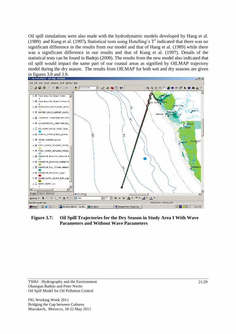
Oil spill simulations were also made with the hydrodynamic models developed by Hang et al.
(1989) and Kung et al. (1997). Statistical tests using Hotelling’s T2 indicated that there was no
significant difference in the results from our model and that of Hang et al. (1989) while there
was a significant difference in our results and that of Kung et al. (1997). Details of the
statistical tests can be found in Badejo (2008). The results from the new model also indicated that
oil spill would impact the same part of our coastal areas as signified by OILMAP trajectory
model during the dry season. The results from OILMAP for both wet and dry seasons are given
in figures 3.8 and 3.9.
Figure 3.7: Oil Spill Trajectories for the Dry Season in Study Area I With Wave
Parameters and Without Wave Parameters
TS06J - Hydrography and the Environment
Olusegun Badejo and Peter Nwilo
Oil Spill Model for Oil Pollution Control
FIG Working Week 2011
Bridging the Gap between Cultures
Marrakech, Morocco, 18-22 May 2011
22/29
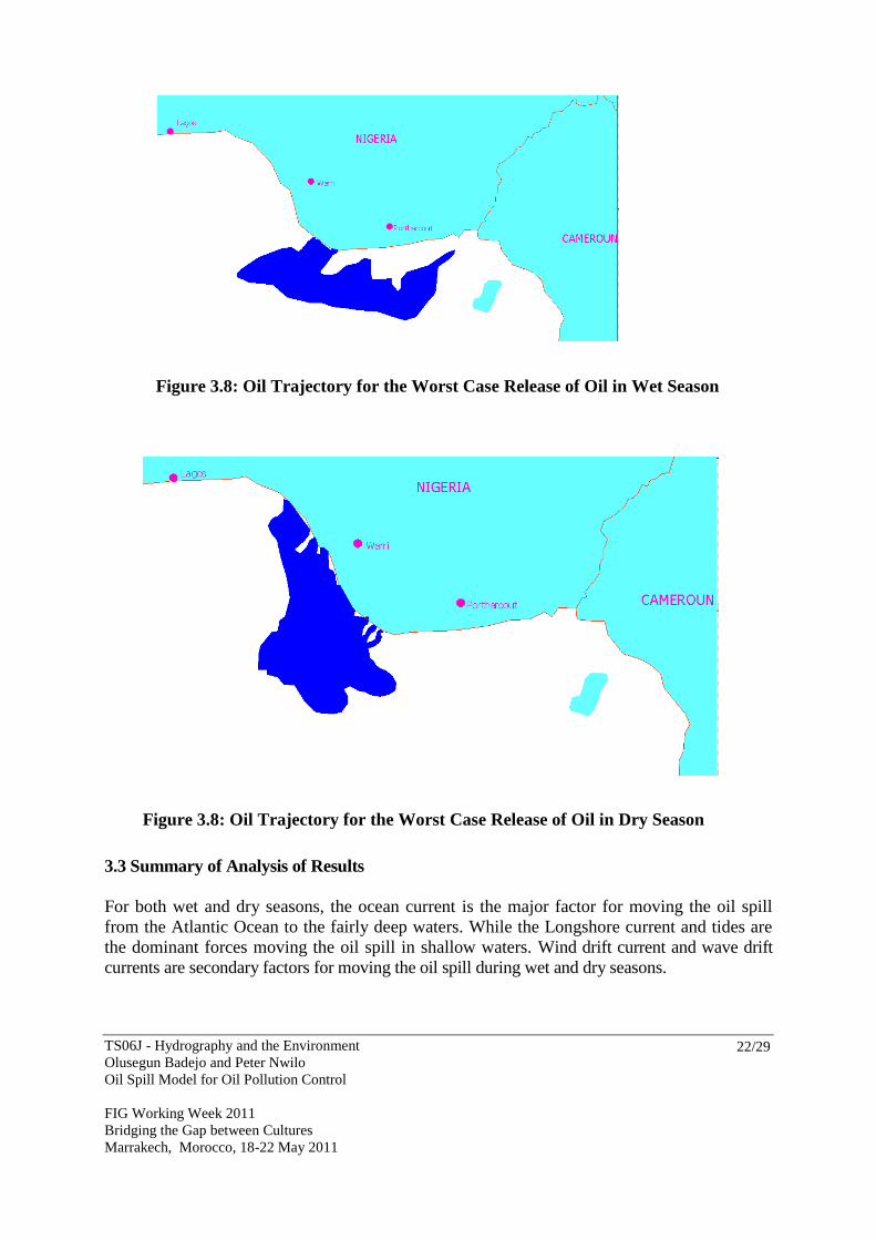
Figure 3.8: Oil Trajectory for the Worst Case Release of Oil in Dry Season
3.3 Summary of Analysis of Results
For both wet and dry seasons, the ocean current is the major factor for moving the oil spill
from the Atlantic Ocean to the fairly deep waters. While the Longshore current and tides are
the dominant forces moving the oil spill in shallow waters. Wind drift current and wave drift
currents are secondary factors for moving the oil spill during wet and dry seasons.
Figure 3.8: Oil Trajectory for the Worst Case Release of Oil in Wet Season

TS06J - Hydrography and the Environment
Olusegun Badejo and Peter Nwilo
Oil Spill Model for Oil Pollution Control
FIG Working Week 2011
Bridging the Gap between Cultures
Marrakech, Morocco, 18-22 May 2011
23/29
The average speed of oil spill on Nigerian coastal waters is 0.29m/s in very deep waters and deep
waters, 0.18 m/s to 0.48m/s in fairly deep waters and 0.31m/s to 0.71m/s along the shoreline
during the wet season.
The bearing of the oil spill varies on Nigerian coastal waters during the wet season. In very deep
waters and deep waters, the average bearing of the oil spill is between 83.09o and 84.58
o. In
fairly deep waters, the average bearing is 66.99o to 135.12
o while the oil spill tend to move along
the coastline along the bearing of the longshore current.
In study area I, the oil spill model indicates that 422,125.548 barrels of oil out of 560,000 spilled
oil would remain after 150 hours during the wet season. This means that 24.62 percent of the oil
would have evaporated by 150hours after the oil spillage. The slick area by this time would be
1656.080sq km.
In study area II, the oil spill model indicates that 439,873.638 barrels of oil out of the 560,000
spilled oil would remain after 131 hours during the wet season. This means that 21.45 percent
of the oil would have evaporated by 131hours after the oil spillage. The slick area by this time
would be 1708.032 sq km.
During the dry season the speed of oil spill is reduced. The speed of oil spill during the dry
season is 0.21m/s to 0.22m/s in very deep waters and deep waters, 0.10m/s to 0.42m/s in fairly
deep waters and 0.25m/s -0.53 m/s along the shoreline. The difference in the speed of the oil
spill for both seasons is due to the fact that the speed of Guinea current (0.23m/s) which is
prevalent during the wet season is higher than that of the Benguela current (0.17m/s) which is
prevalent during the dry season.
The bearing of the oil spill also varies during the dry season. In very deep waters and deep
waters, the bearing of the oil spill is between 16.99o to 20.00
o. In fairly deep waters, the bearing
of the oil spill is between 294.47o to 30.95
o. In shallow waters the oil spill move in the direction
of the longshore current.
During the dry season in study area I, the oil spill model indicates that 347,884.567 barrels of oil
out of the 560,000 spilled oil would remain after 222hours. This means that 37.88 percent of the
oil would have evaporated by 222hours after the oil spillage. The slick area by this time would
be 1432.440sq km.
During the dry season in study area II, The oil spill model also indicates that 507,168.692
barrels of oil out of the 560,000 spilled oil would remain after 56hours. This means that 9.43
percent of the oil would have evaporated by 56 hours after the oil spillage. The slick area by
this time would be 1900.484 sq km.
The wind drift current speed changes with changes in wind speed and water depth. The wind
drift current speed increases with increase in the wind speed, decreases with decrease in water
depth and is deflected by 15 degrees to the right of the bearing of the wind on Nigerian coastal
waters. During the wet season, the wind drift speed is 1.79% of the wind speed in deep water

TS06J - Hydrography and the Environment
Olusegun Badejo and Peter Nwilo
Oil Spill Model for Oil Pollution Control
FIG Working Week 2011
Bridging the Gap between Cultures
Marrakech, Morocco, 18-22 May 2011
24/29
and 0.50% of wind speed in shallow water. During the dry season, the wind drift speed is 1.94%
of the wind speed in deep water and 0.61% of wind speed in shallow water. The increase in the
wind drift speed during the dry season is due to the fact that the speed of the wind is higher
during the dry season. The wind drift speed tends to zero along the coastline.
The wave drift current speed increases as one moves towards the shoreline. The speed of the
wave drift current is 0.003m/s in the Atlantic Ocean, 0.004m/s in deep sea, 0.006m/s in fairly
deep waters and 0.011m/s in shallow waters. The bearing of the wave drift current is 45o on
Nigerian coastal waters. The effects of waves is negligible in very deep waters and deep
waters but cannot be dispensed with in shallow waters.
The effect of tides in very deep waters is negligible. The horizontal speed of tides in the deep
sea is between 0m/s and 0.013m/s. In fairly deep waters and in shallow waters, the horizontal
speed of tide on Nigerian coastal waters varies between 0m/s to 0.22m/s. The bearing of the
tidal waters is 45 degrees during high waters (bearing of the wind) and 225 degrees during
low waters (back bearing of the wind bearing).
Longshore current is a dominant factor for moving the oil spill in shallow waters and along the
coastline. The speed of the longshore current is between 0.16m/s and 0.67m/s and move in
various bearings at different parts of our coastline.
The average rate of evaporation of oil spill is 919.163 barrels of oil per hour during the wet
season and 955.475 barrels of oil per hour during the dry season. The difference of 36.312
barrels of oil per hour during wet and dry season may partly be attributed to the difference in
their wind speed. The wind speed is higher during the dry season. The rate of evaporation of oil
spill is a function of the wind speed and exposure to sunlight.
Statistical analysis using Hotelling’s T2 indicates that the effect of adding waves parameters does
not significantly affect the oil spill result. However, the accuracy of the oil spill model is
improved by adding the wave parameters. Results from this work show that the incorporation of
wave parameters into the oil spill model causes the oil spill to get to the shore a few hours earlier
(one hour during the wet season and eight hours during the dry season for study area one) than
when the wave parameters were neglected in the model. The addition of the wave parameters
also gives additional insight of the additional impact the oil spill will have on coastal wetlands.
The results from the new model also indicated that oil spill would impact the same part of our
coastal areas as signified by OILMAP trajectory model during the dry season.
During the wet season in study area I, the oil sensitivity index map indicates that the oil spill will
pollute and destroy the barrier sands, mangrove forest, mangrove degraded areas and freshwater
degraded region. The oil spill will also pollute rivers, creeks and freshwater between Kulama
River and Ramos River.
During the dry season, the indication we have from the oil sensitivity index maps in study area I
is that the mangrove, mangrove degraded, freshwater degraded and barrier sands would be
TS06J - Hydrography and the Environment
Olusegun Badejo and Peter Nwilo
Oil Spill Model for Oil Pollution Control
FIG Working Week 2011
Bridging the Gap between Cultures
Marrakech, Morocco, 18-22 May 2011
25/29
negatively impacted by oil spill. Benin River, adjacent creeks and freshwater sources will also be
polluted.
In study area II, the oil sensitivity index map indicates that during the wet season, oil spill will
pollute the barrier sands and freshwater degraded region. Rivers, creeks and drinking water
around Eket will also be polluted.
During the dry season in study area II, the oil sensitivity index map indicates that oil spill will
destroy and pollute the freshwater degraded region, freshwater wetlands, barrier sands and
abandoned beach ridges. Rivers, creeks and freshwater supplies between Eket and Imo River will
also be polluted.
4. CONCLUSION AND RECOMMENDATIONS
Conclusion and recommendations based on this work are given in the following sections.
4.1 Conclusion
Some oil spill models have also been deployed to manage oil spill incidents in the country.
However, little success has been achieved in previous efforts to manage oil spill incidents
with these oil spill models. Lack of real time meteorological and historical data, coupled with
inability to develop a model which takes into consideration the full ocean dynamics, waves,
bathymetric of Nigerian coastal waters and peculiar longshore current effects along the
Nigerian coastline led to the little success recorded in managing oil spill incidents on Nigerian
coastal waters.
A new oil spill trajectory model has been developed in this work. The relationship and the
effect of waves induced current in the transport of oil spill on water was considered in the
development of the model. Appropriate wave driven current equation was coupled with that
of wind drift current, ocean current, tidal current and longshore current to generate a new
model for advecting oil spill on coastal waters. Relevant equations for calculating the rate of
spreading and evaporation of oil were also included in the oil spill model to enable the
determination of the fate of oil spill.
The advantages of the model developed in this work are that it is readily available, accurate, as it
has taken into consideration the major factors (including wind drift current, ocean currents,
waves, tides and longshore current) that influence oil spill dispersal on coastal waters. The
attribute of our basemap, which include the environmental sensitivity index maps of the country,
oil blocks, oil and gas wells, bathymetry of the coastal waters and coastal towns and villages
makes it unique. To cap it all, the oil spill trajectory model and the basemap are in the same
ArcGIS environment and file.
4.2 Recommendations

TS06J - Hydrography and the Environment
Olusegun Badejo and Peter Nwilo
Oil Spill Model for Oil Pollution Control
FIG Working Week 2011
Bridging the Gap between Cultures
Marrakech, Morocco, 18-22 May 2011
26/29
The following recommendations if implemented will go a long way in managing and
contolling oil exploitation and exploration activities in the country:
1. There is a need for a better understanding of the coastal ecology so as to evaluate the
significance of the impacts generated by oil spill incidents.
2. The Federal Government in conjunction with oil parastatals and other non-governmental
agencies should create more meteorological stations near the shoreline or on the coastal
waters. The meteorological stations should provide real time or predicted meteorological
data of the surrounding environment. This data would serve among other things as input
data into oil spill models.
3. Medium scale digital maps should be made from satellite images from the Nigeria Sat-1.
Images from the satellite and other satellites such as those from Radar satellites in orbit
could also be used for managing oil spill incidents in the country.
4. Establishment of regional spill response centres along our coastlines, and the use of data
collected with an airborne system will help in managing oil spill problems in Nigeria.
5. Geographic Information System (GIS) could also be used to identify oil spill
responders and provide information about the closest resources of oil spill response
equipment and personnel.
6. The petroleum industry should work closely with government agencies, universities
and research centers and come out with management strategies for combating the
menace of oil spill incidents.
7. More funds should be provided by all the stakeholders in the oil industry for further
research in the development and use of oil spill models in the country. The adoption
and improvement on the model developed in this research work and the procurement
of other oil spill models would serve as a basis in carrying out more research in this
area.
8. When a spill occurs, various governmental and non-governmental agencies should
harness all available resources to reduce the impact of the oil spillage on our coastal
environment.
TS06J - Hydrography and the Environment
Olusegun Badejo and Peter Nwilo
Oil Spill Model for Oil Pollution Control
FIG Working Week 2011
Bridging the Gap between Cultures
Marrakech, Morocco, 18-22 May 2011
27/29
REFERENCES
American Society of Civil Engineers (ASCE), (1996): State of the art review of modelling
transport and fate of oil spills. Journal of Hydrologic Engineering. pp. 594-609.
Applied Science Associates, Inc.(ASA), (1996): Technical Manual for Spill Impact Modeling
(SIMAP), Version W 1.0, Applied Science Associates, Inc, Narragansett, Rl.
Badejo, O.T., (2008): A dynamic mathematical model for oil spill trajectory simulation on
Nigerian coastal waters. Ph.D. Research Thesis. Department of Surveying and
Geoinformatics, University of Lagos, Nigeria. 278pp.
Buranapratheprat, A. & Tanjaaitrong, S., (2000): Hydrodynamic model for oil spill trajectory
prediction. Chulanlongkorn University, Bangkok, Thailand.
Canadian Hydrographic Service, (2005): Tides, Currents and Water Levels. Canadian
Hydrographic Service. Canada.
Dean R.G., & Dalrymple, R.A., (1984): Water waves mechanics for engineers and scientists.
Prentice Hall, Inc Englewood Cliffs, New Jersey. pp. 79.
Delvigne, G. A., (1993): Natural dispersion of oil by different sources of turbulence.
Proceedings of the 1993 international oil spill conference. American Petroleum
Institute, Washington, DC, pp. 415-419.
Delvigne, G. A., Van der Stel, J. A. & Sweeney, C. E., (1987): Final report: Measurement of
vertical turbulent dispersion and diffusion of oil droplets and oiled particles, Delft
Hydraulics Laboratory Report.
Egberongbe, F.O.A., Nwilo, P.C., and Badejo, O.T., (2006a): Oil Spill Disaster Monitoring.
5th FIG Regional Conference, Accra, Ghana. 26 pp.
Fay, J.A., (1971): Physical processes in the spread of oil on a water surface. In proceedings of
the joint conference on prevention and control of oil spills. American Petroleum
Institute, pp. 463-467.
Fay, J.A., (1969): The spread of oil slicks on a calm sea. In oil on the sea. David P. Hoult ed.,
Plenum Press, New York, 53-63.
French M. D., (2006): Oil spill modeling for response planning and impact assessments. US
EPA region III emergency preparedness and prevention and hazard spills conference.
Hang, O., Evensen, P. & Martinsen, E.A., (1989): Oil models for the south China sea.
Technical Report No. 70. Det Norslse Meteorologiske Institutt.
Howlett, E., Jayko, K., and Spaulding, M.L., (1993): Interfacing real time information with
Oil Map. Proceedings of the 16th
Arctic and Marine Oil Spill Program (AMOP),
Technical Seminar, June 7-9, 1993, Edmonton, Alberta, Canada, pp. 539-548.
Kelley, D., (2003): Storm surges. Department of Oceanography, Dalhousie University, Halifax
NS Canada.
Kung, C., Su, K. Chen, Y. & Teng, Y., (1997): Simulation of oil spills in a harbour.
Available at: http://sol.oc.ntu.edu.tw/omisar/wksp.mtg/wom1.97c/rep/rep1-4-3.htm
Lamb, H., (1932): Hydrodynamics. Cambridge University Press, 738pp.
Mackay, D., Peterson, S. & Trudel, K., (1980): A mathematical model of oil spill behavior.
Department of Chemical Engineering, University of Toronto, Canada, 39pp.
Mackay, D. & Matsugu, R. S., (1973): Evaporation rates of liquid hydrocarbon spills on land
and water, Canadian Journal of Chemical Engineering 51, pp. 434-439.

TS06J - Hydrography and the Environment
Olusegun Badejo and Peter Nwilo
Oil Spill Model for Oil Pollution Control
FIG Working Week 2011
Bridging the Gap between Cultures
Marrakech, Morocco, 18-22 May 2011
28/29
McCourt, J., & Shier, L., (2001): Preliminary findings of oil-solids interaction in eight
Alaskan rivers. Proceedings of the 2001 oil spill conference, Washington, D.C.
American Petroleum Institute, pp. 845-849.
McWilliams, J. C., and Sullivan, P.P., (2000): Vertical mixing by langmuir circulations. Spill
and Technology. NOAA Office of Hazardous Materials, in press.
Morales, R. A., Elliot, A. J. and Lunel, T., (1997): The influence of tidal currents and wind on
mixing in the surface layer of the sea. Marine Pollution Bulletin 34, pp. 15-25.
National Academy of Sciences, (2003): Oil in the sea III: Inputs, fates, and effects. 500 Fifth
street N.W. Washigton D.C.
Available at: http://www.national-academies.org/legal/
Nwilo,P.C., and Badejo, O.T., (2006): Impacts and Management of Oil Spill Pollution along
the Nigerian Coastal Areas. In Administering Marine Spaces: International Issues.
FIG Commission 4 and 7 Working Group 4.3 Report. pp. 119 – 133.
Nwilo, P.C., (1995): Sea level variations and the impacts along the Nigerian coastal areas.
Ph.D. Thesis, Environmental Resources Unit, University of Salford, Salford, UK.
Olaleye, J.B., (1992): Optimum software architecture for an analytical photogrammetric
workstation and its integration into a spatial information environment. Technical Report No. 162, Department of Surveying Engineering, University of New Brunswick, Canada, 228 pp.
Officers, C.B., (1976): Physical oceanography of estuaries (and associated coaster waters). John
Wiley and Sons, Inc., UK.
Reddy, G. S. & Brunet, M., (1997): Numerical prediction of oil slick movement in Gabes
estuary. Transoft International, Epinay/Seine, Cedex, France.
Reed, M., (1992): State of the art summary: Modelling of physical and chemical processes
governing fate of spilled oil. Proceedings of the ASCE workshop on oil spill
modeling, Charleston, SC.
Sobey, R.J., & Barker, C.H. (1997): Wave- driven Transport of Surface Oil. Journal of Coastal
Research, 13(2), pp. 490-496. Fort Lauderdale (Florida).
Spaulding, M., (1995): Oil spill trajectory and fate modeling: State-of-the-art review.
Proceedings of the second international oil spill research and development forum,
International Maritime Organization, London, United Kingdom, pp. 508-516.
Stiver, W., & Mackay, D., (1984): Evaporation rate of spills of hydrocarbons and petroleum
mixtures. Environmental Science and Technology 18, pp. 834-840.
Sutton, O. G., (1934): Wind structure and evaporation in a turbulent atmosphere, Proceedings
of the Royal Society of London, A 146, pp. 701-722.
BIBLIOGRAPHY
DR. OLUSEGUN TEMITOPE BADEJO
Dr. O.T. Badejo graduated from the University of Lagos with a Bachelor of Science (B.Sc.)
degree in Surveying in 1992. He also obtained a Master of Science (M.Sc.) degree in
Surveying, in University of Lagos in 1996. His B.Sc. Project was on Sea Level Variation in a
Coastal Seaport, while his M.Sc. research work was on Tidal Prediction Using Least Squares
Approach. Dr. Badejo also has a Ph.D in Surveying and Geoinformatics and he is a Senior

TS06J - Hydrography and the Environment
Olusegun Badejo and Peter Nwilo
Oil Spill Model for Oil Pollution Control
FIG Working Week 2011
Bridging the Gap between Cultures
Marrakech, Morocco, 18-22 May 2011
29/29
Lecturer in Department of Surveying and Geoinformatics, University of Lagos, Nigeria. He is
working on oil spill pollution transport and coastal processes. Dr. O.T. Badejo has over 20
publications.
PROF. PETER CHIGOZIE NWILO
Prof. Nwilo has a Ph.D. in Environmental Resources from the University of Salford, United
Kingdom. He also has a Bachelor of Science and a Master of Science degrees in Surveying
from the University of Lagos. His Ph.D. Thesis is on sea Level Variations and the Impacts
along the Coastal Areas of Nigeria.
He is a registered surveyor, a member of the Nigeria Institution of Surveyors, an Editorial
Board Member of the Journal of Environment Education and Information, University of
Salford, U.K., an Honorary Advisory Board Member of the Encyclopedia of Life Support
System and an Editorial Board Member of the African Geodetic Journal. Prof. Nwilo had a
fellowship Award of the European Community for his Ph.D.; and was a Federal Government
of Nigeria scholar for his M.Sc. and B.Sc. degrees.
Dr. Nwilo has over 70 publications in journals and conferences in the areas of surveying,
coastal management, oil spill, sea level variations, subsidence and environmental
management.
CONTACTS
Dr. Olusegun T. Badejo & Prof. Peter C. Nwilo
Department of Surveying and Geoinformatics
University of Lagos
Lagos
NIGERIA
Tel: 2348038636448, 2348035725644
Email: [email protected], [email protected]