Embed Size (px)
Citation preview

OLG-CGE Models and Demographic Research
Robert E. Wright
Professor of Economics
University of Strathclyde
Presentation, “CGE Modelling for Policy Analysis-International Cases”, University of Helsinki Ruralia
Institute, Seinajoki, Finland, March 16-17, 2015

Financial support from the Economic and Social Research Council under the grant: “Developing an OLG-CGE Model for Scotland” is gratefully acknowledged.
Additional financial support was provided by the University of Ottawa and the University of Strathclyde.

COLLABORATORS
OLG-CGE Modelling of Demographic Change
• Katya Lisenkova, National Institute of Economic and Social Research, London
• Marcel Merette, Department of Economics, University of Ottawa
• Jokke Kinnunen, Statistics and Research Åland
CGE Modelling of Demographic Change
• Peter McGregor, University of Strathclyde
• Kim Swales, University of Strathclyde
• Nikos Pappas, Government of Greece
• Karen Turner, University of Strathclyde
• Patrizio Lecca, University of Strathclyde
• Kristinn Hermannsson, University of Glasgow

Overview
1. Motivation
2. Scottish Background
3. OLG-CGE Models
4. Three Sets of Results
5. Concluding Comments

1. Motivation
• Population ageing is the shift in the age-structure away from the younger to older age groups
• It is occurring in almost all countries
• Most “rich” countries are ageing rapidly
• Increase in the number/share of population aged 65 and older
• Decrease in the number/share of population aged 20 and younger
• Low, no or slow growth in the number/share of population aged 20 to 64 years
• Population ageing is NOT population decline

Figure 1
Age Distribution, Scotland, 1911
15 10 5 0 5 10 15
0-4
5-9
10-14
15-19
20-24
25-29
30-34
35-39
40-44
45-49
50-54
55-59
60-64
65-69
70-74
75-79
80-84
85+
Age g
roup
Percentage of total population
Men
Women
Figure 4
Age Distribution, Scotland, 2041
15 10 5 0 5 10 15
0-4
5-9
10-14
15-19
20-24
25-29
30-34
35-39
40-44
45-49
50-54
55-59
60-64
65-69
70-74
75-79
80-84
85-89
90+
Ag
e g
rou
p
Percentage of total population
Men
Women

• “Accommodating” population ageing will be (is) expensive in
welfare states
• Increase in the “demand” for state-supplied pensions and other age-
related benefits targeting at older people
• Big expected increases in government expenditure
• Big expected increases in taxes to pay for it
• Need “high” economic growth if ∆T > ∆G
• If not…

• Dominant view is that population ageing “suppresses” economic
growth
• Why? One main reason is slow/no/low labour force growth
• Welfare state: Those “in work” pay for those “not in work”
• Difficult “political economy” in democratic countries with “one man,
one vote” systems
• “Greying of the electorate coupled” with a steep upwards sloping
relationship between age and political participation
• Significant standard of living reductions likely

Policy options?
1. Increase immigration
2. Introduce/expand “family friendly” policies
3. Raise the “age of retirement”
4. Increase spending on education and human capital investment
5. “Older age” employment subsidies
6. Subsidise/expand research and development activities
7. “Focus” on capital-intensive industries
8. Improve the cost-effectivness of government
9. Do nothing
10. Do nothing and “hope” for a technological leap

2. Scottish Background

1,00
1,50
2,00
2,50
3,00
3,50
1950 1960 1970 1980 1990 2000 2010 2020 2030 2040 2050 2060
Figure 1Total Fertility Rate, Scotland and UK, 1951-2062
Scotland UK

60,0
65,0
70,0
75,0
80,0
85,0
90,0
95,0
1950 1960 1970 1980 1990 2000 2010 2020 2030 2040 2050 2060
Figure 2Life Expectancy at Birth, Scotland and UK, 1951-2062
Scotland Men Scotland Women UK Men UK Women

-50 000
-40 000
-30 000
-20 000
-10 000
0
10 000
20 000
30 000
40 000
195
1
195
3
195
5
195
7
195
9
196
1
196
3
196
5
196
7
196
9
197
1
197
3
197
5
197
7
197
9
198
1
198
3
198
5
198
7
198
9
199
1
199
3
199
5
199
7
199
9
200
1
200
3
200
5
200
7
200
9
201
1
201
3
201
5
201
7
201
9
202
1
202
3
202
5
202
7
202
9
203
1
203
3
203
5
203
7
203
9
204
1
204
3
204
5
204
7
204
9
205
1
205
3
205
5
205
7
205
9
206
1
Figure 3Net-migration, Scotland, 1951-2062

-100
-80
-60
-40
-20
0
20
40
60
80
100
1950 1960 1970 1980 1990 2000 2010 2020 2030 2040 2050 2060
Figure 4Net-migration rate (per 10,000 population), Scotland and UK, 1951-2062
UK Scotland

100
105
110
115
120
125
130
2010 2015 2020 2025 2030 2035 2040 2045 2050 2055 2060 2065
Figure 5Projected Population, Principal Projection, Scotland and UK, 2012-2062 (2012=100)
Scotland UK

80
85
90
95
100
105
110
115
120
2010 2015 2020 2025 2030 2035 2040 2045 2050 2055 2060 2065
Figure 7Projected Population Aged 20-64, Principal Projection, Scotland and UK, 2012-2062
(2012=100)
Scotland UK

40,0
45,0
50,0
55,0
60,0
65,0
70,0
75,0
80,0
85,0
2010 2015 2020 2025 2030 2035 2040 2045 2050 2055 2060 2065
Figure 14Unadjusted and Adjusted Total Dependency Ratio, Principal Projection,
Scotland and UK, 2012-2062
Total UK Scotland
Adjusted UK Adjusted Scotland
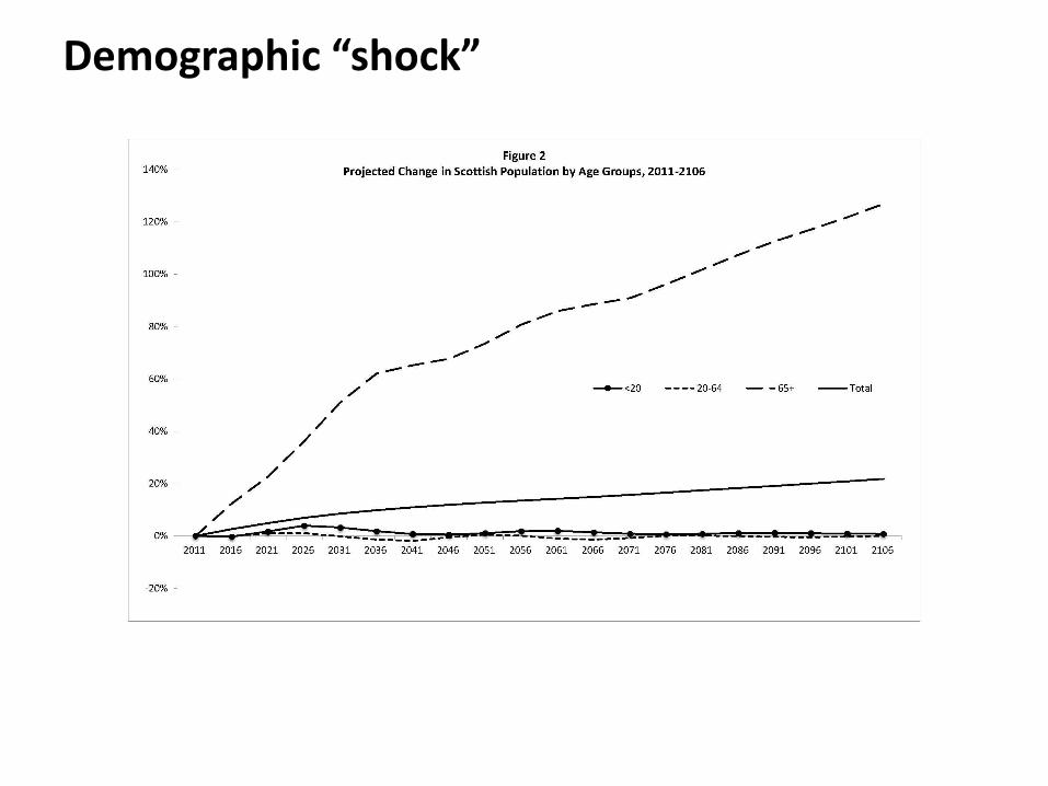
Demographic “shock”

3. OLG-CGE Models
OLG = “over-lapping generations”
CGE = “computable general equilibrium”

What are CGE Models?
• A computer general equilibrium (CGE) model is a description of aneconomy using a system of simultaneous equations
• The “general equilibrium” idea implies that all the markets, sectorsand industries are modelled together with corresponding inter-linkages
• This is opposed to “partial equilibrium” that only takes intoaccount a part of the system (e.g. labour market), which neglectspotential feed-backs
• This mathematical representation, coupled with a solver algorithm,ensures the “computable” nature of the model i.e. empirical resultsare generated

• Models can be used for “what if” simulations thereby allowing one
to obtain numerical results for endogenous variables based on
assumptions about exogenous variables, functional forms, and
parameter values
• Most CGE models rest on neo-classical economic assumptions
• Consumers are assumed to maximise their utility subject to a budget
constraint (demand-side)
• Producers are assumed to maximise profit, given the prices of goods
and factor of production costs (supply side)
• For each good and factor of production, equilibrium price is
calculated where that demand equals supply

• The first CGE model was constructed by Johansen in 1960.
• Have been largely used to analyse the macro-economic effects of a
large number of economic policies such as liberalising foreign trade,
decreasing government expenditure and increasing taxation.
• Main strength of CGE models lies with their flexibility, in the sense
that their “general” nature means that they can be adapted to a variety
of problems depending on the creativity and ingenuity of the
researcher.
• CGE modelling is an “art”

CGE models are not in a strict sense a forecasting models.
However, given a set of precise assumptions, it can be used to
generate expected future time paths of key macroeconomic
variables:
Output, employment, unemployment, labour force participation,
investment, wage rates, inflation and competitiveness.
By varying these assumptions alternative time paths are
produced, which can be compared in order to evaluate the likely
consequences of alternative policies.

Some Useful Features:
Substitution in production or consumption
Non-passive supply side i.e. both demand and supply considered so
“supply matters” (no the case in I-o)
Relative prices become endogenous (e.g. the real wage and regional
competitiveness are determined within the model)
Producers and consumers allowed to respond to relative price changes
through substitution in production or demand
More flexible technology and demands structures (non-linearities)

• More flexible technology and demands structures (non-
linearities)
• Over lapping generations (OLG) structure makes them more
“demographically friendly”
• Can be used to “price” shocks, changes and policies e.g. In £s
or per cent output loss
• Consistency with microeconomic “circular flow”
underpinnings.

Figure 1. Micro-economic “Circular Flow”
Firms
Households
Factor
Mrkts
Goods
Mrkts

Computable
Calibration
Accuracy is evaluated by back “forecasting” (backcasting)

• Not surprising that more recently such model have been applied to a
series demographic problems largely (but not exclusively) around the
impacts of population ageing
• The type of CGE model that is best suited to demographic research
builds in the notion of “over lapping generations” (OLG-CGE)
• This approach more explicitly allows the interaction of age effects,
which in most demographic problems is of central importance.

Firm-side
One sector. One good. Cobb-Douglas production function
Factor prices equal to their marginal product
Labour demand disaggregated by types of labour
Three types of assets
Household assets
Government assets
Foreign assets
One region (RUK only to close the model)

Household-side • 21 generations – from 0-4 to 100+
– First 4 generations only affect public consumption
– Starting from 20-24 generations optimise their consumption/savings
• Four types of households depending on level of qualification– Three working qualifications (high, medium, low)
– One non-working
• Two types of nationalities– British born
– Foreign born
• Age/qualification-specific productivity (age-earnings profiles)
• Age-specific labour force participation rates

Overlapping generations structure
A1 A2 A3 A4 A5
T1 G1
T2 G2 G1
T3 G3 G2 G1
T4 G4 G3 G2 G1
T5 G5 G4 G3 G2 G1
T6 G6 G5
T7 G7 G5
T8 G8 G5
T9 G9 G5
T10 G10 G9 G8 G7 G6
T11 G11 G10
T12 G12 G10
T13 G13 G10
T14 G14 G10
Age
Tim
e

Demography: Standard approach
• Generations are “born” when they enter labour force
• They live for certain number of years
• At specified age they die with certainty
• Fixed (certain) life expectancy
• One variable parameter – “fertility rate”

Problems with standard approach
Population structure is a result of three demographic
processes
– Fertility (people appear at the beginning)
– Migration (people appear/disappear in the middle)
– Mortality (people disappear in the middle and at the
end)

Why use standard approach?
Certainty is required to use standard household optimisation problem
Household Utility Function
Household Budget Constraint
Euler Equation
a
at
a
cU
1)1(
1 1
1
Aa+1,t+1 = Aa,t (1+ rt+1)+Wa,t -Ca,t
Ca+1,t+1
Ca,t,
=1+ rt+1
1+ r
æ
èç
ö
ø÷
1/q

Demography: Our Approach
Variable “mortality” rate (includes both mortality and migration)
Life expectancy uncertainty on individual level but not on generation level, as mortality schedule is known today and at every point in time in the future
Perfect annuity market (accidental bequests distributed implicitly)
Alternative –bequests distributed between children (e.g., Hans Fehr, Sabine Jokisch, Laurence J. Kotlikoff, 2003, 2004, 2005)

New household problem
• Household Utility Function
• Household Budget Constraint
a
ta
taa
a
csU
1)1(
11
,
,1
Aa+1,t+1 =1
sa,t
Aa,t (1+ rt+1)+Wa,t -Ca,t( )
sa,t -- probability of survival for age a at time tsa,t=popa+1,t+1/popa,t

New household problem
• Household Utility Function
• Household Budget Constraint
• Euler Equation
a
ta
taa
a
csU
1)1(
11
,
,1
Aa+1,t+1 =1
sa,t
Aa,t (1+ rt+1)+Wa,t -Ca,t( )
Ca+1,t+1
Ca,t,
=1+ rt+1
1+ r
æ
èç
ö
ø÷
1/q
sa,t -- probability of survival for age a at time tsa,t=popa+1,t+1/popa,t
Government revenues
• Two taxes– Wage tax
– Consumption tax
• Separate pension contributions
• Return on government assets
• UK fiscal transfer

Government expenditures
• Three types of public consumption
1. Age-independent (fixed level per capita)
2. Health expenditures (mostly for old age)
3. Education expenditures (mostly for young age)
• Transfers (qualification-specific)
• Pensions (for 65+ year old)

Age-specific public expenditures• At the moment calibrated on the National Transfer
Accounts (NTA) for Canada
• NTA measure economic flows across age groups in a manner consistent with National Accounts. This is a very new approach to measuring intergenerational transfers
• UK NTAs are in the process of preparation– David McCarthy and James Sefton at Imperial college
represent the UK in the NTA project
– First estimates of UK National Transfer Accounts (April 2011)


Age-related components of the model
• Age-specific labour force participation rates
• Age-qualification-specific productivity profile
• Age-specific government spending on health and education
• Age-specific consumption profile (from calibration stage)

ASIDE: Ageing and Consumption
A key part of the ageing impacts puzzle is missing:
(1) Consumption of almost any good or service differs by age
(2) Age-consumption profile is inverted U- or J-shaped
• With population ageing there will be increases in demand for some goods/services and decreases in demand for other goods and services
• “Average” consumption increases and then decreases with age
• Clear supply-side effects.
• Requires multi-sector modelling

5. Results 1: Size versus Age-specific Effects
• Hypothesis: Relative importance of “size” versus “age-specific effects"
• Demographic shock: “ONS 2010-based principal population projection”
• Run model with age-specific effects “turned off”
• Run model with age-specific effects “turned on”
• Macro-economic variable of interest: Output per person


5. Results 2: Immigration and Economic Growth
• “Grow” the labour force
• Hypothesis: Relative importance of different levels of net migration
• Demographic shock: “2010-based variant population projection with
different level of net-migration”
• Run model with different levels of net-migration
• Macro-economic variable of interest: Output per-person

Additional Assumptions
Levels of net-migration:
1. Zero
2. 10,000
3. 20,000
4. 30,000
5. 40,000
6. 50,000
Sex ratio: 50% female, 50% male
Age structure of immigration: < age 45 distributed equally


5. Results 3: Do Nothing and “Hope” for Technological
Change
How big of a leap is needed?
What rate of technological change is needed

“Solow Residual” estimate of TFP growth
• Rise in output with constant capital and labour
• Rate of growth in total factor productivity
• Not an “explanation”
• Growth accounting exercise or growth decomposition
• Question: What causes the residual?

Estimate of TFP growth
Solow (1957): USA, 1909-1949, 1-2% per year
Maddison (1987): 1950-1973, France 4.0%
Germany 4.3%
Japan, 5.8%
UK, 3.1%
USA, 1.9%
Kohli and Werner (1997): Korea, 1971-1991, 3.5%
1971, 4.2%
1991, 2.4%

Technological “shocks”
Positive shocks “steepens” the production function
Examples of “big” shocks:
1. Information technology/computing “revolution”
Krueger (1993): USA, 1984-1989: Wages 10-15% higher for jobs that
involve using PCs
2. Reduction in shipping costs: Wind-to coal-powered freight ships
3. Large reductions in mortality: Labour productivity increase “caused”
by improved health. “Healthy workers are more productive workers”,
increased participation, increased labour supply

• Baseline scenario: circa 15% welfare loss
• How much technological change is needed to counteract this welfare
loss?
• Arithmetic suggests total factor productivity growth of 0.14% year is
needed to keep output per-person constant
• Over the past two decades in the UK total productivity growth over
the past two decades has averaged around 2% per year
• So about 7% of the recent past historical growth is needed.

• Technological change needed to counteract population ageing is
considerable.
• What is going to be the source of this change?
• Complications:
“Age-bias” in technological change
“Skill-bias” in technological change

6. Concluding Comments?

Special issue of Journal of Economic Modelling
Volume 35, 2013

“Demographic Applications of Over-lapping Generations
Computable General Equilibrium (OLG-CGE) Models”
Giorgio Garau, Patrizio Lecca and Giovanni Mandras, “The Impact of Population
Ageing on Energy Use: Evidence from Italy”
Katerina Lisenkova, Marcel Mérette and Robert Wright, “Population Ageing and the
Labour Market: Modelling Size and Age-specific Effects”
Patrick Georges, Katerina Lisenkova and Marcel Mérette, “Can the Ageing North
Benefit from Expanding Trade with the South?”
Axel Börsch-Supan and Alexander Ludwig, “Modelling the Effects of Structural
Reforms and Reform Backlashes: The Cases of Pension and Labour Market Reforms”

CGE-OLG Demographic Modelling Teams/Research
Groups
Department of Economics, University of Ottawa: Marcel Mérette
National Institute for Economic and Societl Research: Katya Lisenkova
Max Planck Institute for Social Law and Social Policy: Axel Börsch-Supan
Vienna Institute of Demography: Alexia Fürnkranz-Prskawetz
INGENUE Team, France: CEPII, CEPREMAP, MINI-University of Paris X and OFCE:
Vincent Touze
Department of Human and Social Sciences, University of Calgliari: Giorgio Garau
Ministry of Economy, Trade and Industry: Kazuhiko Oyamada
Regional Economic Applications Laboratory, University of Illinois at Urbana-Champaign:
Geoff Hewings
Department of Economics, Loyola University, Seville, Alejandro Cardenete