Olivier Blanchard April 2007 - MIT OpenCourseWare · Olivier Blanchard April 2007 Nr. 1 Cite as: Olivier Blanchard, course materials for 14.452 Macroeconomic Theory II, Spring 2007

14.452. Topic 3, continued. RBCs

Olivier Blanchard

April 2007

Nr. 1 Cite as: Olivier Blanchard, course materials for 14.452 Macroeconomic Theory II, Spring 2007. MIT OpenCourseWare (http://ocw.mit.edu/), Massachusetts Institute of Technology. Downloaded on [DD Month YYYY].

RBC model naturally fits co-movements output, employment, productivity,consumption, and investment.Success? Not yet:

Labor supply elasticities: plausible? •

Technological shocks. Are they really there? •


1. Movements in employment and the labor/leisure choice

Under log-log, the elasticity of employment with respect to the wage, • given consumption, is given by:

dN = −

dL L = −

dL 1 − N =

1 − N dwN L N L N N w

If we assume (like King-Rebelo) that N ¯ = .2 (that we spend 20% of our • time working), then η = 4.

If we assume that N ¯ = .5 (we spend half of our available time working),• then η = 1

Empirical estimates (of which there are many in the micro-labor lit) are • all much lower, below 1.

If assume η = 1, then, as shown in Figure 8 of King-Rebelo, we do not• get much action in employment relative to the data.


Figure removed due to copyright restrictions.Figure 8: Consequences of smaller shocks and smaller labor elasticity on page 965.King, R. and S. Rebelo. "Resuscitating Real Business Cycles." Chapter 14 in Handbook of Macroeconomics. Vol. 1B. Edited by J. Taylor and M. Woodford. New York, NY: Elsevier, 1999, pp. 927-1007. ISBN: 9780444501578.


(2) Intensive versus extensive margins

Above: all at the intensive margin (hours). Most of the (cyclical) action • at the extensive margin: work or not work (bodies) : U(C, N), N = 0 or 1

If all workers have the same reservation wage, then labor supply fully elastic at that wage, up to full employment.

Still an income effect. At a given wage, labor supply shifts up if consumption increases.

• Complication 1. If different histories, different consumption, different reservation wages.

Thus, an aggregate labor supply curve with slope. No tight relation between individual and aggregate labor supply.


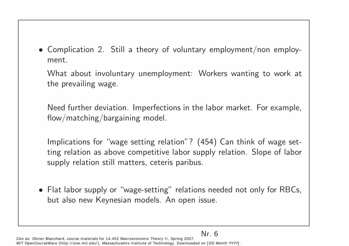
• Complication 2. Still a theory of voluntary employment/non employment.

What about involuntary unemployment: Workers wanting to work atthe prevailing wage.

Need further deviation. Imperfections in the labor market. For example, flow/matching/bargaining model.

Implications for “wage setting relation”? (454) Can think of wage setting relation as above competitive labor supply relation. Slope of labor supply relation still matters, ceteris paribus.

Flat labor supply or “wage-setting” relations needed not only for RBCs, • but also new Keynesian models. An open issue.


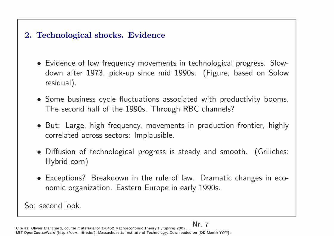
2. Technological shocks. Evidence

Evidence of low frequency movements in technological progress. Slow• down after 1973, pick-up since mid 1990s. (Figure, based on Solow residual).

Some business cycle fluctuations associated with productivity booms. • The second half of the 1990s. Through RBC channels?

• But: Large, high frequency, movements in production frontier, highly correlated across sectors: Implausible.

• Diffusion of technological progress is steady and smooth. (Griliches: Hybrid corn)

• Exceptions? Breakdown in the rule of law. Dramatic changes in economic organization. Eastern Europe in early 1990s.

So: second look.


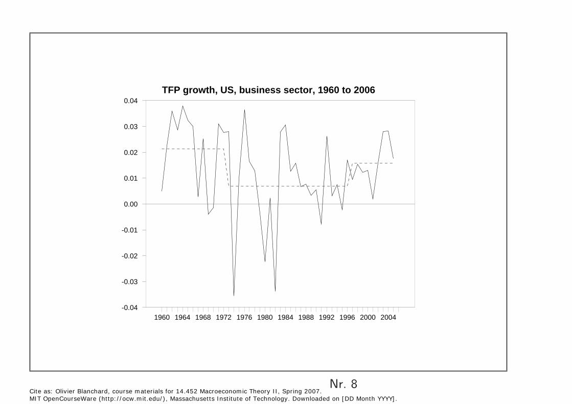
TFP growth, US, business sector, 1960 to 2006

1960 1964 1968 1972 1976 1980 1984 1988 1992 1996 2000 2004-0.04

-0.03

-0.02

-0.01

0.00

0.01

0.02

0.03

0.04


Image removed due to copyright restrictions.

Nr. 9Cite as: Olivier Blanchard, course materials for 14.452 Macroeconomic Theory II, Spring 2007. MIT OpenCourseWare (http://ocw.mit.edu/), Massachusetts Institute of Technology. Downloaded on [DD Month YYYY].

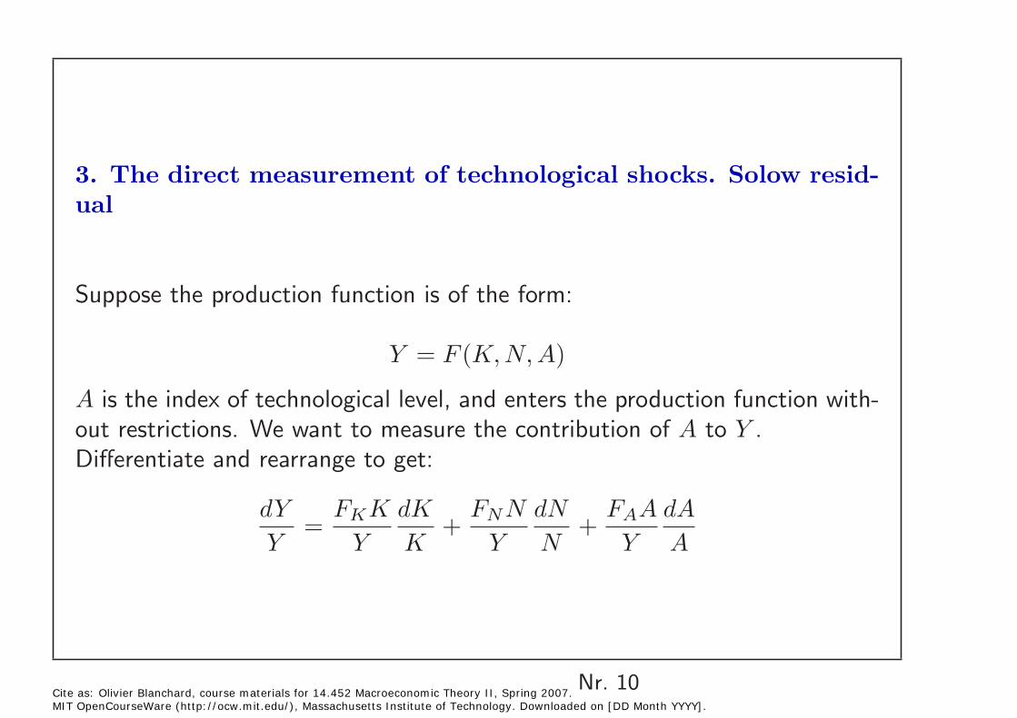
3. The direct measurement of technological shocks. Solow residual

Suppose the production function is of the form:

Y = F (K, N, A)

A is the index of technological level, and enters the production function without restrictions. We want to measure the contribution of A to Y . Differentiate and rearrange to get:

dY FK K dK FN N dN FAA dA = + +

Y Y K Y N Y A


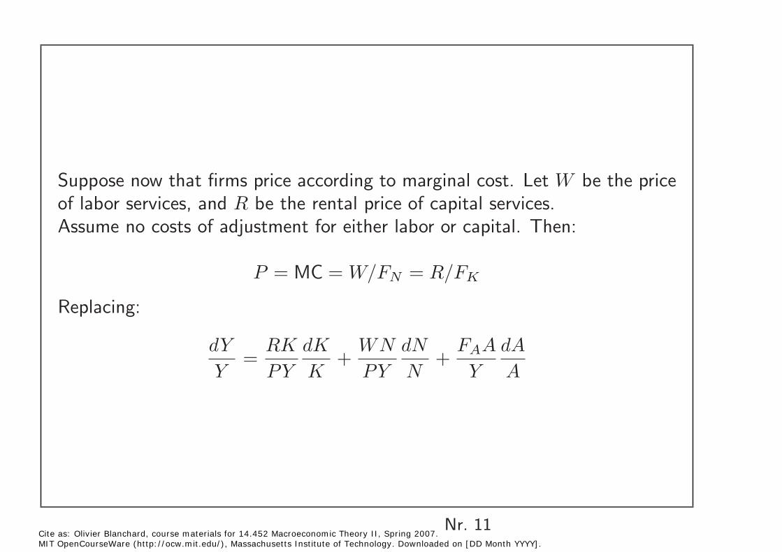
Suppose now that firms price according to marginal cost. Let W be the priceof labor services, and R be the rental price of capital services.Assume no costs of adjustment for either labor or capital. Then:

P = MC = W/FN = R/FK

Replacing:

dY RK dK WN dN FAA dA = + +

Y PY K PY N Y A


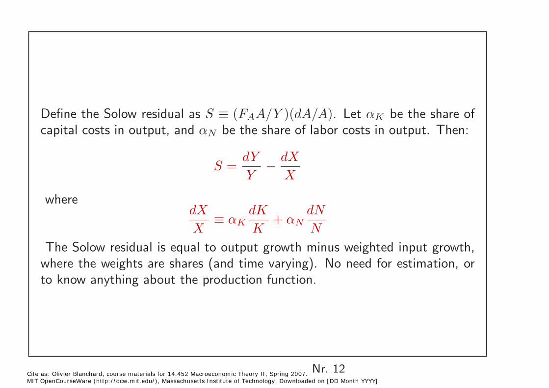
Define the Solow residual as S ≡ (FAA/Y )(dA/A). Let αK be the share of capital costs in output, and αN be the share of labor costs in output. Then:

dY dX S =

Y −

X

where dX dK dN ≡ αK + αNX K N

The Solow residual is equal to output growth minus weighted input growth, where the weights are shares (and time varying). No need for estimation, or to know anything about the production function.


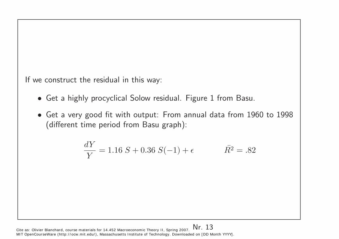
If we construct the residual in this way:

Get a highly procyclical Solow residual. Figure 1 from Basu. •

Get a very good fit with output: From annual data from 1960 to 1998 • (different time period from Basu graph):

dY ¯= 1.16 S + 0.36 S(−1) + � R2 = .82 Y

Cite as: Olivier Blanchard, course materials for 14.452 Macroeconomic Theory II, Spring 2007. Nr. 13MIT OpenCourseWare (http://ocw.mit.edu/), Massachusetts Institute of Technology. Downloaded on [DD Month YYYY].

�


Figure removed due to copyright restrictions. Figure 1 in Basu, S., J. Fernald., and M. Kimball. “Are Technology Improvements Contractionary?” Federal Reserve Bank of Chicago, WP-2004-20.

Solow used this approach to compute S over long periods of time. Reasonable to construct it to estimate technological change from year to year, or quarter to quarter? The answer is: Probably not. A number of serious problems. Among them:

Costs of adjustment. If costs of adjustment to capital, then the shadow • rental cost is higher/lower than the rental price R.

Same if costs of adjustment to labor. So shares using rental prices or wages may not be right.

Non marginal cost pricing. Firms may have monopoly power, in which • case, markup µ will be different from one.

• Unobserved movements in N or K. Effort? Capacity utilization?


Examine the effects of the last two (markups, and unobserved effort or capacityutilization)

(On costs of adjustment just to capital, no problem. Condition still holds forlabor, so use the share of labor to weight the change in employment. And useone minus the share of labor to weight the change in capital.More of an issue if costs of adjustment to both.)


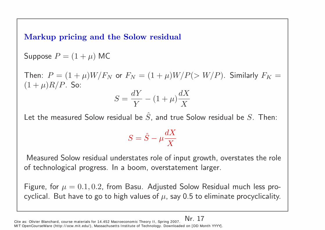
Markup pricing and the Solow residual

Suppose P = (1 + µ) MC

Then: P = (1 + µ)W/FN or FN = (1 + µ)W/P (> W/P ). Similarly FK = (1 + µ)R/P . So:

dY dX S = − (1 + µ)

Y X

Let the measured Solow residual be S, and true Solow residual be S. Then:

dX S = S − µ

X

Measured Solow residual understates role of input growth, overstates the role of technological progress. In a boom, overstatement larger.

Figure, for µ = 0.1, 0.2, from Basu. Adjusted Solow Residual much less pro-cyclical. But have to go to high values of µ, say 0.5 to eliminate procyclicality.


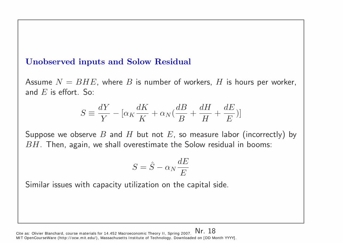
Unobserved inputs and Solow Residual

Assume N = BHE, where B is number of workers, H is hours per worker, and E is effort. So:

dY dK dB dH dE S ≡

Y − [αK

K + αN (

B +

H +

E )]

Suppose we observe B and H but not E, so measure labor (incorrectly) by BH. Then, again, we shall overestimate the Solow residual in booms:

S = ˆ dES − αN

E Similar issues with capacity utilization on the capital side.


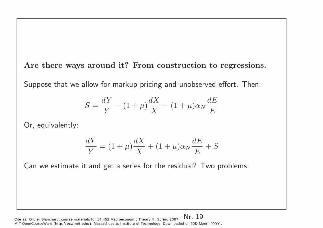
Are there ways around it? From construction to regressions.

Suppose that we allow for markup pricing and unobserved effort. Then:

dY dX dE S = − (1 + µ) − (1 + µ)αN

Y X E

Or, equivalently:

dY dX dE= (1 + µ) + (1 + µ)αN + S

Y X E

Can we estimate it and get a series for the residual? Two problems:


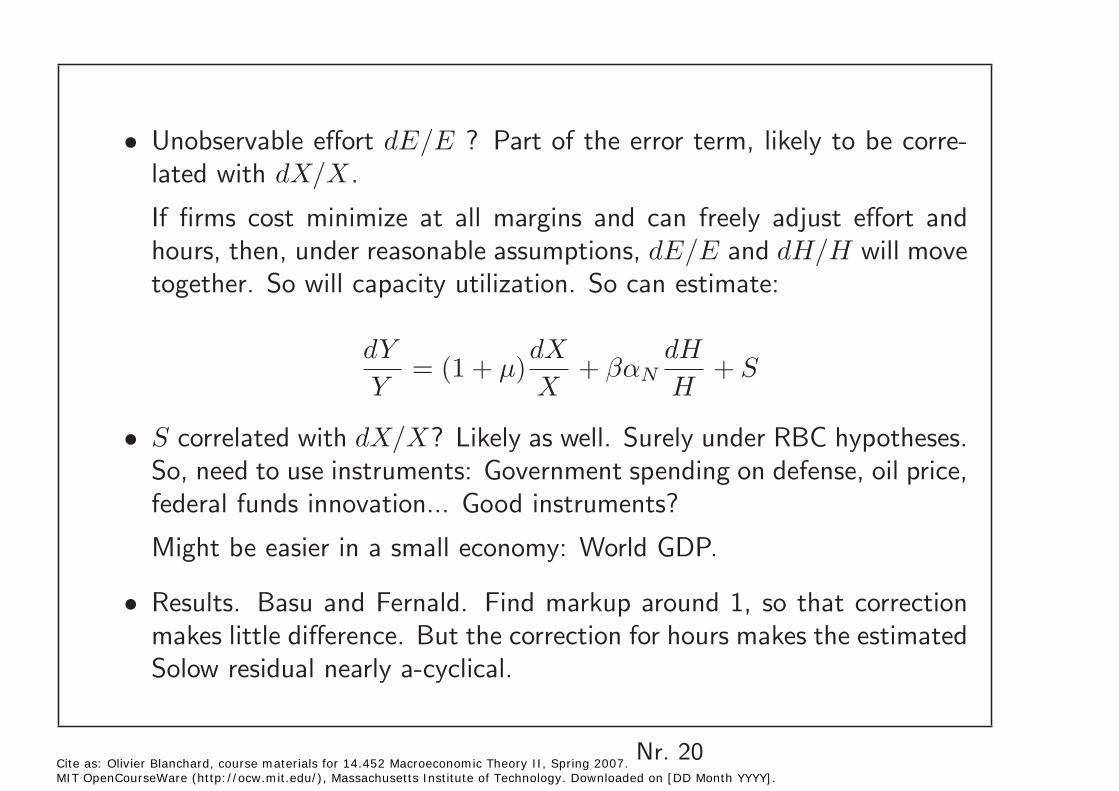
Unobservable effort dE/E ? Part of the error term, likely to be corre• lated with dX/X.

If firms cost minimize at all margins and can freely adjust effort andhours, then, under reasonable assumptions, dE/E and dH/H will movetogether. So will capacity utilization. So can estimate:

dY dX dH= (1 + µ) + βαN + S

Y X H

Scorrelated with dX/X? Likely as well. Surely under RBC hypotheses. • So, need to use instruments: Government spending on defense, oil price,federal funds innovation... Good instruments?

Might be easier in a small economy: World GDP.

• Results. Basu and Fernald. Find markup around 1, so that correction makes little difference. But the correction for hours makes the estimated Solow residual nearly a-cyclical.



Image removed due to copyright restrictions.

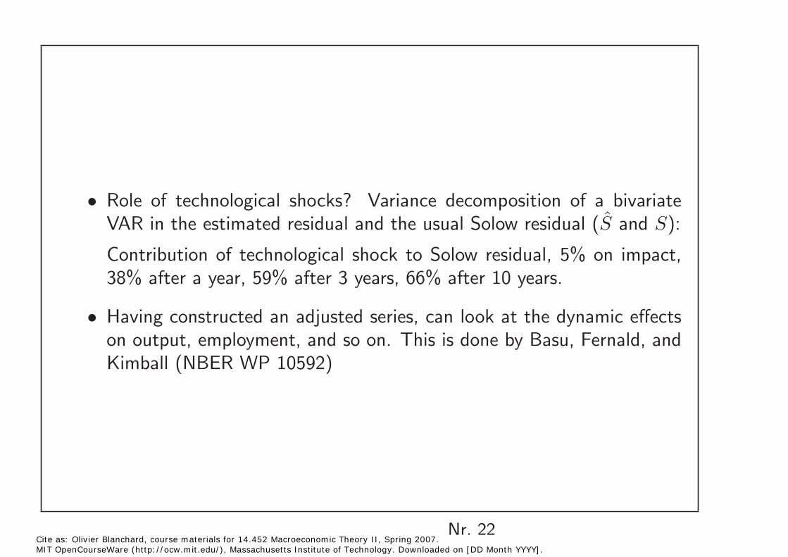
• Role of technological shocks? Variance decomposition of a bivariate VAR in the estimated residual and the usual Solow residual ( S and S):

Contribution of technological shock to Solow residual, 5% on impact, 38% after a year, 59% after 3 years, 66% after 10 years.

Having constructed an adjusted series, can look at the dynamic effects • on output, employment, and so on. This is done by Basu, Fernald, and Kimball (NBER WP 10592)


Figure removed due to copyright restrictions. Figure 3 in Basu, S., J. Fernald., and M. Kimball. "Are Technology Improvements Contractionary?” Federal Reserve Bank of Chicago, WP-2004-20.


4. An alternative SVAR approach

An alternative construction of shocks, and the results. Gali 2004 (building onBlanchard Quah 1989).Identify the technological shocks as those shocks with a long term effect onproductivity, and then trace their short run effects on output, employment,productivity.Technically:

Estimate a bivariate VAR in Δ log(Y/N) and Δ log(N). Stationary. So• no effect of shocks on productivity growth and employment growth. But potential effects on level of productivity, and level of employment.

Assume two types of shocks. •

Shocks with permanent effects on level of productivity.

Shocks with no permanent effects on level of productivity.

This is sufficient for identification.


Increase in output, but less than productivity. So a (small) decrease inemployment (measured by total hours worked).

Figure removed due to copyright restrictions.Figure 2: The Estimated Effects of Technology Shocks in Gali, J. and P. Rabanal. “Technology Shocks and Aggregate Fluctuations: How Well does the RBC Model Fit Postwar U.S. Data?”In NBER Macroeconomics Annual 2004. Edited by M. Gertler and K. Rogoff. Cambridge, MA: MIT Press, pp. 225-318. ISBN: 9780262572293.


______________________________

http://mitpress.mit.edu/catalog/item/default.asp?ttype=2&tid=10523

Figure removed due to copyright restrictions.Figure 3: Sources of U.S. Business Cycle Fluctuations in Gali, J., and P. Rabanal.“Technology Shocks and Aggregate Fluctuations: How Well does the RBC Model Fit Postwar U.S. Data?” In NBER Macroeconomics Annual 2004. Edited by M. Gertler and K. Rogoff. Cambridge, MA: MIT Press, pp. 225-318. ISBN: 9780262572293.


______________________________


How robust? Controversial, but my reading: fairly robust. •

See discussion in Gali. (Gali 1992 finds a larger role for technological shocks at cyclical frequencies).

• An independent confirmation. Basu et al (2004) trace the effects of their constructed measure of technological shocks on output, employment. See above. Also find an initially negative effect of the shocks on employment.

Relation between the two sets of shocks? Quite good. Figure. •


Figure removed due to copyright restrictions. Figure 5: Technology Shocks: VAR vs. BFK in Gali, J. and P. Rabanal. “Technology Shocks and Aggregate Fluctuations: How Well does the RBC Model Fit Postwar U.S. Data?” In NBER Macroeconomics Annual 2004. Edited by M. Gertler and K. Rogoff. Cambridge, MA: MIT Press, pp. 225-318. ISBN: 9780262572293.


______________________________


5. Idiosyncratic versus aggregate technological shocks.

Plausible that technological shocks large at firm/sector level even at highfrequency, but law of large numbers limits their importance at aggregate level

Gabaix (2005) for a theoretical and empirical counterargument.•

• Franco and Philippon (“Firms and aggregate dynamics”, http://ssrn.com/abstract=640584) for supporting evidence

SVAR approach. Look at a panel of firm, allowing firms to be affected by permanent shocks to technology, permanent shocks to relative demand, and common aggregate (demand?) shocks.

Find a large role for permanent shocks to technology at the firm level, largely washing out in the aggregate.


Summary

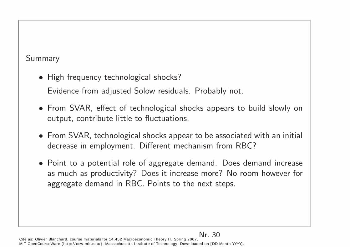
High frequency technological shocks? •

Evidence from adjusted Solow residuals. Probably not.

From SVAR, effect of technological shocks appears to build slowly on• output, contribute little to fluctuations.

From SVAR, technological shocks appear to be associated with an initial• decrease in employment. Different mechanism from RBC?

Point to a potential role of aggregate demand. Does demand increase• as much as productivity? Does it increase more? No room however for aggregate demand in RBC. Points to the next steps.


Documents

Olivier Blanchard April 2007 - MIT OpenCourseWare · Olivier Blanchard April 2007 Nr. 1 Cite as: Olivier Blanchard, course materials for 14.452 Macroeconomic Theory II, Spring 2007