olutionary Rates Across Gradients

Acc

epte

d A

rtic

le

This article has been accepted for publication and undergone full peer review but has not been

through the copyediting, typesetting, pagination and proofreading process, which may lead to

differences between this version and the Version of Record. Please cite this article as doi:

10.1111/2041-210X.12419

This article is protected by copyright. All rights reserved.

Received Date : 07-Jul-2014

Revised Date : 20-Mar-2015

Accepted Date : 29-May-2015

Article type : Research Article

Editor : Liam Revell

Evolutionary Rates Across Gradients

Jason. T. Weir1,2

and Adam Lawson1

1) Department of Biological Sciences and Department of Ecology and Evolutionary biology,

University of Toronto Scarborough, Toronto, ON, M1C 1A4, Canada

2) E-mail: [email protected]

Abstract

1) A key question in the fields of macroecology and evolution is how rates of evolution vary

across gradients, be they ecological (e.g. temperature, rainfall, net primary productivity),

geographic (e.g. latitude, elevation), morphological (e.g. body mass), etc. Evolutionary

rates across gradients (EvoRAG 2.0) is a new software package provided as open source

in the R language (and available from CRAN) that tests whether rates of trait evolution

vary continuously across such continuous gradients.

Acc

epte

d A

rtic

le


2) The approach uses quantitative trait data for a series of sister pair contrasts (i.e. sister

species or other types of sister taxa) and applies Brownian Motion and Ornstein

Uhlenbeck models in which parameter (evolutionary rate and constraint) values vary as a

function of discrete variables (e.g. male versus female) and/or continuous variables (e.g.

latitude, temperature, body size).

3) We used simulation to test performance of the models in EvoRAG. Our gradient models

accurately estimate parameter values, have very low levels of bias, and low rates of

model misspecification.

4) The modelling framework developed here provides great flexibility in designing models

that test how rates of evolution vary across gradients. We provide an example where both

discrete (songbird versus suboscine) and continuous (latitude) effects on evolutionary rate

in avian song were simultaneously estimated.

Key-words: Evolutionary rates, continuous character, gradients, Brownian Motion, Ornstein

Uhlenbeck, bird song, song learning

Introduction

Investigation of the rates and patterns of trait evolution along dated molecular phylogenies is

now common thanks to the development of a number of packages in the R and other languages

(e.g. auteur, Eastman et al. 2011, ape, Paradis et al. 2004; BAMM, Rabosky 2014; geiger,

Harmon et al. 2008; motmot, Thomas & Freckleton 2012; OUCH, King & Butler 2009; OUwie,

Beaulieu & O’Meara 2012; 2012; phytools, Revell 2012; RBrownie, Stack et al. 2011; and

Acc

epte

d A

rtic

le


others). Many studies investigating trait evolution aim to uncover how evolutionary rates have

changed through the radiation of a focal clade by testing for slowdowns in rate that might be

indicative of adaptive radiation (e.g. Harmon et al. 2010, Rabosky 2014) or identifying subclades

that may have experienced rate shifts in association with the evolution of key innovations (e.g.

Eastman et al. 2011; Jønsson et al. 2012; Rabosky 2014; Revell et al. 2012). One method

(Brownie, O’Meara et al 2006) allows separate evolutionary rates to be applied to species that

occur in different discrete categorical states independent of where such species occur on a

phylogeny. This method is useful for determining if the state of a discrete character influences

rates of evolution in another continuous character. However, many interesting evolutionary

questions involve the influence of gradients, rather than discrete characters. Here we provide a

complementary approach that allows rates of evolution for a continuous trait to vary, not only

between categorical states as in Brownie, but also as a function of a continuous gradient. The

method tests the hypothesis that rates of evolution vary as a function of the gradient. Though

models have been developed to test whether rates of molecular evolution are associated with

other continuous variables like body size (e.g. Lartillot & Poujol 2010; Lanfear, Welch &

Bromham 2010), a more general modelling framework for non-molecular characters is needed.

The method we introduce uses sister pair contrasts (sister species or other sorts of sister

taxa) to estimate evolutionary rates. Sister pair data provide a snapshot of how evolution

proceeded near the tips of a phylogeny, and avoids what often are unreasonable assumptions

from whole tree approaches about how evolution may have proceeded at deeper levels in a

phylogeny, where, in the absence of a detailed fossil record, trait data will be lacking. The

method developed here is appropriate for datasets in which each sister pair has an estimated age

Acc

epte

d A

rtic

le


of divergence (using molecular or fossil data), a Euclidean distance (or other distance metric) in

a trait of interest (the trait for which evolutionary rates will be calculated), and data for a gradient

along which differences in rates of evolution in the trait of interest will be tested. The method is

coded into a new R package, EvoRAG: Evolutionary Rates Across Gradients. Here we describe

the modelling framework of EvoRAG, test model performance, and provide advice on how to

generate each of the components of a dataset. We then present a worked example in which

evolutionary rates in bird song are allowed to vary between different discrete subsets (two

taxonomic suborders), and within each subset, to vary as a function of a continuous

environmental variable (the midpoint latitude of each sister pair).

Model Description

EvoRAG currently employs Brownian Motion (BM) and Ornstein Uhlenbeck (OU) models of

trait evolution to sister pair data. The BM model describes a random walk in trait space through

time with an instantaneous dispersion parameter, β (i.e. the evolutionary rate, also commonly

referred to as σ2). The expectation is that a species trait value will, on average, remain the same

as the starting trait value, but the variance in trait value increases as a product of time and β. This

increase in variance through time is unbounded in BM (i.e. trait space has no limitations).

Clearly, unbounded evolution is unrealistic for many trait spaces, in which case an OU model

may more accurately reflect evolutionary dynamics. In addition to β, the OU model adds a

parameter, α, which provides a constraint on evolution, so that trait divergence becomes more

difficult as a species diverges further from a central trait value (often referred to as the optima).

As α increases, divergence away from this central trait value becomes more difficult. α can thus

Acc

epte

d A

rtic

le


be seen as a stabilizing selective force or as a measure of the degree of evolutionary constraint.

As α approaches zero, the model collapses to the BM model.

Our approach uses sister pair data by modelling trait divergence (D) between species within a

sister pair (i):

Di = X1i- X2i eqn 1

where X1i and X2i are the mean trait values for each species in a sister pair. The set of Di is

normally distributed with expectation (mean) zero and with variances (see Felsenstein 1973):

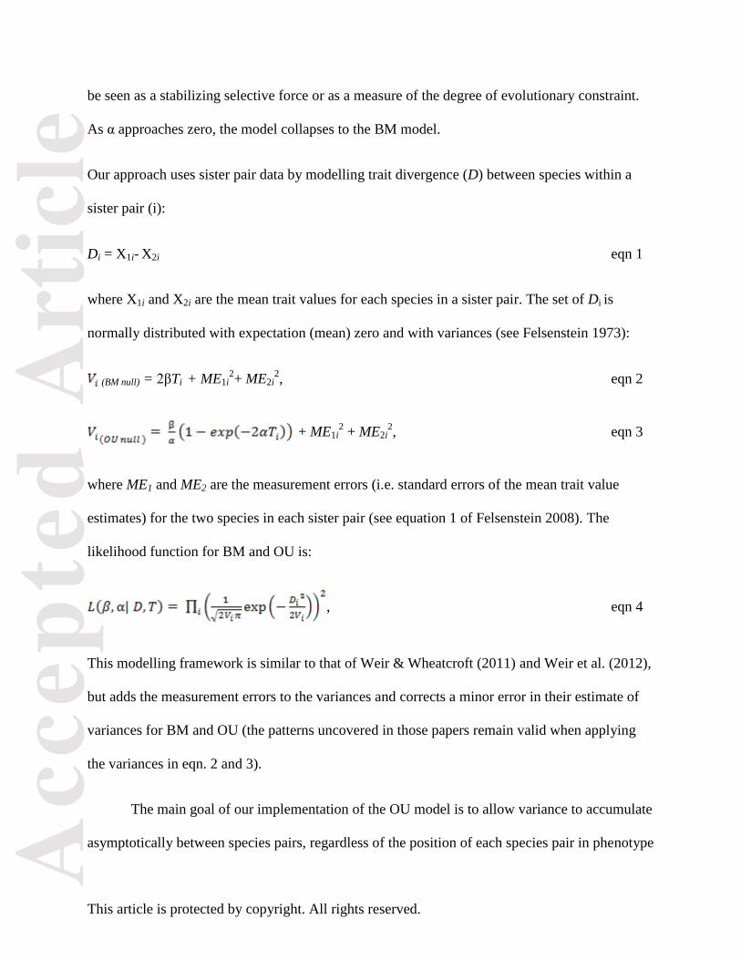
(BM null) = 2βTi + ME1i2+ ME2i

2, eqn 2

+ ME1i2 + ME2i

2, eqn 3

where ME1 and ME2 are the measurement errors (i.e. standard errors of the mean trait value

estimates) for the two species in each sister pair (see equation 1 of Felsenstein 2008). The

likelihood function for BM and OU is:

, eqn 4

This modelling framework is similar to that of Weir & Wheatcroft (2011) and Weir et al. (2012),

but adds the measurement errors to the variances and corrects a minor error in their estimate of

variances for BM and OU (the patterns uncovered in those papers remain valid when applying

the variances in eqn. 2 and 3).

The main goal of our implementation of the OU model is to allow variance to accumulate

asymptotically between species pairs, regardless of the position of each species pair in phenotype

Acc

epte

d A

rtic

le


space. To do this, we assume that all sister pairs have their own optimal values in trait space,

which are identical to the trait values of the ancestors for each pair. Allowing each sister pair its

own optimum is useful for the type of comparative analysis that EvoRAG is suited for, because

most sister pair datasets will pool sisters from many different clades, each of which are likely to

occupy different regions of trait space. In essence, this is a model analogous to stabilizing

selection, where divergence away from the ancestral trait value for each sister is penalized by α.

However, because the method implemented here models trait divergence between species rather

than individual trait values for each species, the ancestor states and the optima do not appear in

equation 4 and are not estimated by the model.

The expected (i.e. mean) absolute trait divergence after a given amount of time has

passed is:

, eqn 5

and follows a half normal distribution. The EvoRAG function expectation.time takes a set of

parameters for the BM or OU models and plots the expected mean and quantiles through time.

Here we illustrate these expectations with a few examples to help compare the workings of the

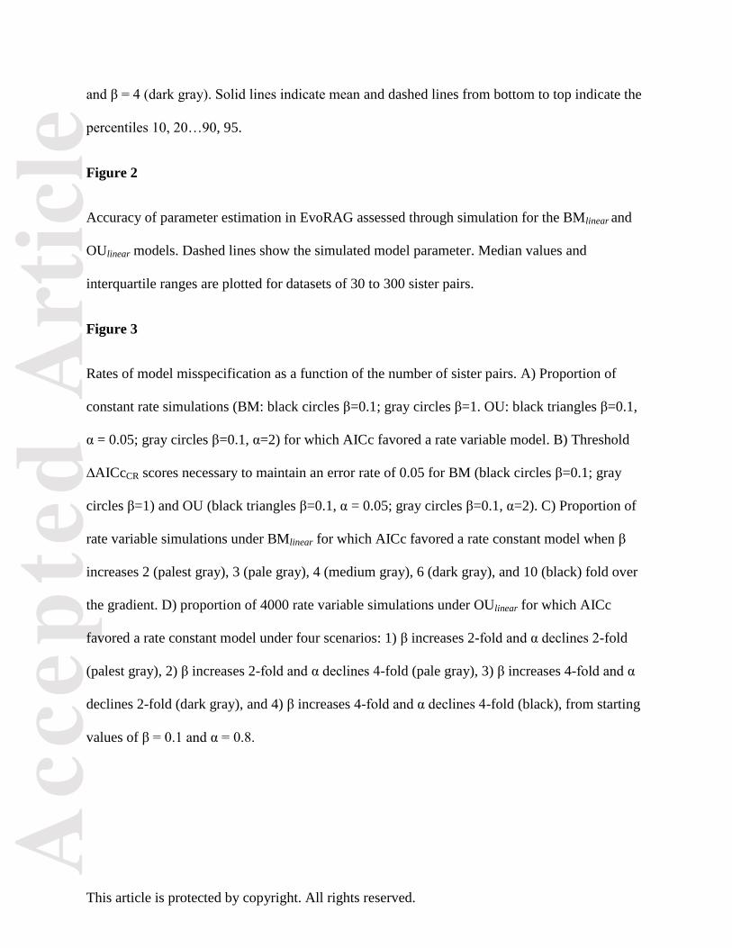
BM and OU models. Figure 1a plots the expectation under BM when β = 1, with data simulated

under that model for comparison. At T = 0, the expectation of |D| is 0, and then increases

indefinitely through time, but not in a linear fashion. Doubling the evolutionary rate increases the

expectation at any time point, but does not result in a doubling of the expectation (β = 2, Fig. 1b).

This is important, because datasets with significantly different evolutionary rates may not always

appear to differ greatly upon visual inspection. Under the OU model, the expectation approaches

an asymptote when α > 0 (Fig. 1c). Once the expectation has closely approached the asymptote,

Acc

epte

d A

rtic

le


the expectation will not continue to increase greatly through time. The asymptote is determined

by both α and β. When β is held constant and α increases, the asymptote occurs at lower values

of |D| and is approached more rapidly (Fig. 1c versus d). When α is held constant and β

increases, the asymptote occurs at higher values of |D| (Fig. 1d versus e).

In addition to implementing models where β and α are constant across all species (BMnull and

OUnull), EvoRAG allows β and α to vary as a function of a second continuous variable, G, using

the following three models:

1) BMlinear: β changes as a linear function of G (β is replaced with in eqn. 1). The

model has 2 parameters.

2) OUβ-linear: same as BMlinear but with a constant rate of α across the gradient. The model

has 3 parameters.

3) OUlinear: both β and α change as a linear function of G. (β is replaced with and

α is replaced with in eqn 1). The model has 4 parameters.

EvoRAG allows model parameters to vary as other functions of G (e.g. quadratic), but these are

not detailed here.

The function expectation.gradient plots the expected |D| across the gradient (G), after a given

amount of time has passed (set by the user). This function is useful for exploring the effects of

the gradient on trait divergence. This is especially useful for the OUlinear model where change in

β and α may be positively correlated across a gradient, making it less clear whether there is an

increase or decrease in expected |D| across the gradient. For example, if β and α both increase

across a gradient, the expected |D| may decline across the gradient, despite the increase in

Acc

epte

d A

rtic

le


evolutionary rate. Studies using the OUlinear model may benefit from reporting the maximum

likelihood estimate of the gradient in expected |D|, rather than just β.

Model Performance

The simulation function in EvoRAG, sim.sisters, uses the same approach as in packages like

geiger (Harmon et al. 2008) and diversitree (Fitzjohn 2012) to simulate trait data along the

branches of a phylogeny. In our case, each simulated sister pair is represented by a phylogeny

having only two tips, a single node, and with ancestor state 0. The resulting simulated trait data

at the tips are then transformed into D values. Data can be simulated under the rate constant

models (BMnull and OUnull) and under gradient models (BMlinear, OUβ-linear, OUlinear). Simulation

was used to assess model performance (parameter re-estimation, model bias, type I error and

statistical power) along a gradient that spanned 0 to 60 (as is applicable to a latitudinal gradient

extending from the equator to the boreal). Six datasets were used that differed in the number of

sister pairs (n = 30, 60, 90, 120, 150 and 300 sister pairs), with sisters divided evenly across 5

latitudes (0°, 15°, 30°, 45°, 60°) in each. Sister pairs at each latitude were divided evenly across

6 ages typical of sister species datasets (0.5, 1, 1.5, 2, 4, 8 million years).

Parameter Re-estimation: Simulation was used to determine if models provided reasonable

estimates of parameters. For each model, 1000 sets of D were simulated for an arbitrary trait

(BMnull: beta = 0.1; OU-null: beta =0.1, alpha=0.8; BMlinear: beta at 0° = 0.1, beta at 60° = 0.2;

OUβ-linear: beta at 0° = 0.1, beta at 60° = 0.2, alpha = 0.8; OUlinear: beta at 0° = 0.1, beta at 60° =

0.2, alpha at 0° = 0.8, alpha at 60° = 0.4) for each of the six datasets. The same model used to

Acc

epte

d A

rtic

le


simulate trait data was then used to obtain the maximum likelihood estimate of model parameters

for each simulation. All models in EvoRAG provided similar median estimates of parameter

values as they were simulated under (data shown only for BMlinear and OUlinear in Fig. 2). The

interquartile range of parameter re-estimates declined as the number of sisters increased,

indicating that larger sample sizes should result in increased accuracy of parameter estimates.

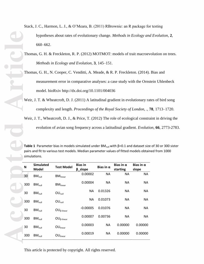
Model Bias: To test for model bias we simulated 1000 datasets under BMnull with β = 0.1 for our

datasets with 30 and 300 sister pairs. Simulations were then fit to the other models (BMlinear,

OUβ-linear, OUlinear), and median values of parameter estimates under these models were obtained.

Bias occurs when parameters not present in BMnull are estimated to be non-zero using the other

models. No appreciable bias was found in any model parameter (Table 1). For example, the

median α parameter of the OUnull model was small (0.01) and slope parameters of the gradient

models were very small, indicating low bias. These results contrast with those of a recent study

which used similar methods to show that the α parameter of OU models is biased when using

some whole tree approaches (Thomas et al. in press). While we are uncertain why some whole

tree approaches find a bias while our sister pair approach does not, one possibility is that the

need to estimate the ancestor state in whole tree approaches, or their utilization of a single

optima for all species in a tree may result in the described biases.

Rates of Model Misspecification: The methods in EvoRAG are designed to test models in

which rates of evolution are constant (BMnull, OUnull) versus models in which rates vary across a

gradient (BMlinear, OUlinear_beta, OUlinear).The model with the lowest AICc (Akaike Information

Criterion adjusted for sample size) is chosen as the best fit of the candidate models to the data.

Acc

epte

d A

rtic

le


We used simulation to determine rates at which a rate variable model is incorrectly specified by

AICc when the data is simulated under a rate constant model. 4000 sets of D for an arbitrary trait

were simulated for each of the six datasets for BMnull (β = 0.1, and 1) and OUnull (β = 0.1, α=0.5

and 2.0). Each simulated set was fit to the rate constant models (BMnull, OUnull) and to the three

rate variable models (BMlinear, OUlinear_beta, OUlinear), and AICc was used to determine whether a

rate variable or rate constant model was best supported. The proportion of simulations for which

a rate variable model was incorrectly chosen as the best fit model is shown in Fig. 3a and ranges

between 0.15 and 0.2.

Models with AICc values less than 2 units above the best fit model (∆AICc = 2) are often

considered to have substantial support along with the best supported model, while models with

AICc values greater than 2 units are considered as receiving weaker support and are often not

considered further (e.g. Burnham & Anderson 2001). Figure 3b shows the necessary ∆AICc

value required to maintain a model misspecification rate of 0.05. These ∆AICc values are similar

or slightly higher than the usual cut-off value of 2 units for these simulated datasets.

We also used simulation to determine rates at which a rate constant model is incorrectly

specified by AICc when the data is simulated under a rate variable model. Rates of model

misspecification for rate variable models are expected to decrease with increasing number of

sister pairs in a dataset and with increasing effect of the gradient on β and α. For each of the six

datasets varying in the number of sister pairs, 500 sets of D for an arbitrary trait were simulated

under each gradient model for the following sets of parameters. BMlinear: β at 0° = 0.1, β at 60° =

2, 3, 4, 6, and 10x higher than at 0°. OUβ-linear: the same as for BMlinear, but with alpha = 0.5.

OUlinear: four scenarios were used. Scenario 1: β at 0° = 0.1, β at 60° = 2x higher, α at 0° = 0.8, α

at 60° = -2x lower. Scenario 2: same as scenario 1 but with α at 60° = -4x. Scenario 3: same as

Acc

epte

d A

rtic

le


scenario 1 but with β at 60° = 4x. Scenario 3: same as Scenario 3, but with α at 60° = -4x. Each

simulated dataset was fit to each constant rate model and to each variable rate gradient model.

The proportion of simulations for which a rate constant model was incorrectly chosen as

the best fit model is shown in Fig. 3c and d. As expected, model misspecification decreased with

increasing values of n, as well as increasing effect of the gradient on parameters. BMlinear and

OUβ-linear exhibited almost identical rates of model misspecification (results are shown in Fig. 3c

only for BMlinear), suggesting that the addition of α (which is constant across the gradient in OUβ-

linear) does not affect model misspecification. For these models, a two-fold increase in β across

the gradient had low rates of model misspecification only with a dataset of N=300. Conversely,

when β increased 10-fold, datasets with as few as 30 sisters had low rates of model

misspecification. When the effect of the gradient is strong, datasets with as few as 30 sister pairs

may be sufficient. When smaller gradient effects are expected, low rates of model

misspecification will be retained only with larger dataset sizes.

For the OUlinear model, both the effect of the gradient on α and β influences model

misspecification (Fig. 3d). A two-fold increase in β and two-fold decrease in α only achieved

low rates of model misspecification with n=90 to 120 or higher. Both a two-fold increase in β

and four-fold decrease in α, or a four-fold increase in β and two-fold decrease in α had low rates

of model misspecification above n=60. A four-fold increase in β and four-fold decrease in α had

low model misspecification above n=60, but even with n=30, rate constant models were

incorrectly favored only in 10% of simulations. These results suggest that even with just four-

fold changes in α and β, datasets as small as 30 sister pairs should provide sufficiently low rates

of model misspecification.

Acc

epte

d A

rtic

le


The Software

Input Data: EvoRAG uses sister pair data. These may represent sister species or deeper sister

clades in a phylogeny, provided sister pairs are not phylogenetically nested. The user supplies a

dataset of sister pair ages (T), distances between species (either D or |D| will work in equation

4), and values for the continuous character (G) over which β and α will be allowed to vary. Here

we comment on strategies for measuring T, D, and G.

T: Sister pair ages will generally be obtained from molecular data, but could also be timespans

from fossil data. If age estimates are obtained from ultrametric molecular phylogenies (which do

not need to be calibrated), then T for each sister pair is equal to its node age. If age estimates are

obtained from sequence divergence between sister pairs, then T is equal to half the sequence

divergence. If fossil data is used, then care must be taken that sister taxa within a sister pair are

each drawn from the same time period as assumed by equations 1 to 4. Likewise, branch lengths

from non-ultrametric phylogenies cannot be used.

|D|: Euclidean distances are generally calculated on the mean or midpoint trait value for each

species in a sister pair. Species mean trait values calculated from a limited sample size or with

measurement error may greatly misrepresent the population mean. As a result, |D| are generally

biased upwards by low sample sizes. When the true distance between species are small (i.e.

intraspecific variation is large relative to interspecific variation), this bias can have a strong

effect on estimated Euclidean distances, and could be especially important for recently diverged

sister pairs (see Harmon & Losos 2005). For this reason, we strongly suggest that intraspecific

sampling be maximized and standard errors of the sampling mean be obtained. For species with

only a single individual measured, intraspecific variances obtained for other species in the

Acc

epte

d A

rtic

le


dataset can be used to estimate standard errors. These standard errors can then be incorporated

into equations 2 and 3. Standard errors assume that individuals have been sampled at random. If

sampling is non-random (e.g. geographically aggregated, as is often true for museum data), then

the standard error correction may not be valid. An alternative approach is to use midpoints rather

than mean trait values. Provided care has been taken to sample broadly across a species

geographic range (i.e. one approach is to sample populations from opposite sides of a species

range), midpoint values will help avoid biases generated by aggregated sampling.

G: The gradient can be environmental (e.g. temperature, rainfall), geographic (e.g. latitude,

longitude, elevation), ecological (e.g. net primary productivity), morphological (e.g. body mass)

etc. Currently, five publish studies using EvoRAG have used either latitude (Weir & Wheatcroft

2011; Weir et al. 2012; Lawson & Weir 2014), the degree of climatic divergence (Lawson &

Weir 2014), the degree of sexual dimorphism (Seddon et al. 2013), or relative testes size (Rowe

et al. 2015) scored as a continuous character as their gradient. G for each sister pair can be

calculated in several ways depending on the question of interest. For the published studies using

latitude, sexual dimorphism and testes size, G was calculated as the absolute midpoint between

the gradient scores for each individual species in a pair, under the assumption that sisters diverge

in their gradient scores in a Brownian motion fashion. This approach is useful if the question of

interest is to determine if rates of evolution vary as a function of the gradient value. Because

some sisters may have diverged greatly from their ancestral trait value along the gradient, it may

be reasonable to include only sister pairs in which both members of a sister pair have reasonably

similar gradient values. For example, for a latitudinal gradient, it makes little sense to use the

midpoint latitude for a species pair in which one species occurs in the arctic and the other near

the equator, because the midpoint latitude for the pair would occur in areas where neither species

Acc

epte

d A

rtic

le


currently exist. For this reason, limits should be imposed on how different species within a

species pair are allowed to be in their gradient values for inclusion in a dataset. In the case of

previous studies with latitude (and the example that follows in the next section), midpoint

latitudes of species in a pair could differ by no more than 20° latitude for inclusion (Weir et al.

2012). Alternatively, if the question of interest is whether rates of evolution vary as a function of

divergence in another character (i.e. an evolutionary gradient), then G would be calculated as the

absolute difference between the gradient values for each species (see Lawson & Weir 2014).

The maximum likelihood search: The key function in EvoRAG is model.test.sisters which

allows users to fit the above models to their data using maximum likelihood. model.test.sisters

returns a matrix of the fitted models that includes the log-likelihood, Akaike Information

Criterion (AIC and AICc), and parameter estimates.

Testing data subsets: Different data subsets may support different rates for the same model, or

even support different models. These subsets might be defined by different taxonomic groupings,

occupation of different habitats, allopatric versus sympatric pairs etc. To test whether a subset is

significantly supported, the models in model.test.sisters should be fit to the entire dataset without

the subset and then separately to each data subset. The log-likelihood for the subsets model is

simply the sum of the log-likelihood for each of the subsets, and the resulting AIC value will

reflect the increased number of parameters that results from fitting the models separately to each

subset. The AIC for the subsets model can then be compared to the AIC when fit to the entire

dataset (see Worked Example below).

Acc

epte

d A

rtic

le


Confidence Intervals: Confidence intervals can be constructed in two ways. First, the function

bootstrap.test uses bootstrap resampling of the dataset to determine confidence intervals using

the percentile method. Second, profile likelihood (Profile.like.CI) can be used to calculate

confidence intervals on a parameter by parameter basis. Both methods should generally work

well. However, the likelihood surface may form a ridge between α and β under the OU

framework in some datasets, and in such cases, profile likelihood may do a better job delimiting

confidence intervals when such ridges occur.

Simulation Capabilities: EvoRAG allows data to be simulated under any of the models

implemented. These can be used to test for rates of model misspecification and to determine

appropriate ∆AICc thresholds.

Worked Example

Here we illustrate the use of EvoRAG with a previously published dataset on avian syllable

diversity for 116 New World species pairs of passerine birds (Weir & Wheatcroft 2011).

Euclidean distances (|D|) were derived from principal component 2 in Weir & Wheatcroft which

represents an axis of syllable diversity. Species pairs with high Euclidean distance have songs

with very different numbers of syllable types per song. The relative age of each sister pair (T) is

estimated as half the genetic distance separating each member of the sister. Full details of this

worked example are provided in a supporting online tutorial to this manuscript.

First, we illustrate the use of EvoRAG for a discrete test of evolutionary rate differences

between two major suborders of passerines: the suboscines (52 sister pairs), for which most

components of song are believed to have a strong genetic component, and the songbirds (64

Acc

epte

d A

rtic

le


sister pairs) for which many aspects of song (including syllable formation) have a strong

culturally learned component (e.g. Baptista 1996). Song learning is generally believed to elevate

rates of song evolution in songbirds, because errors in song learning and innovation can rapidly

introduce new syllable types. To test these predictions, we compared rates of song learning in

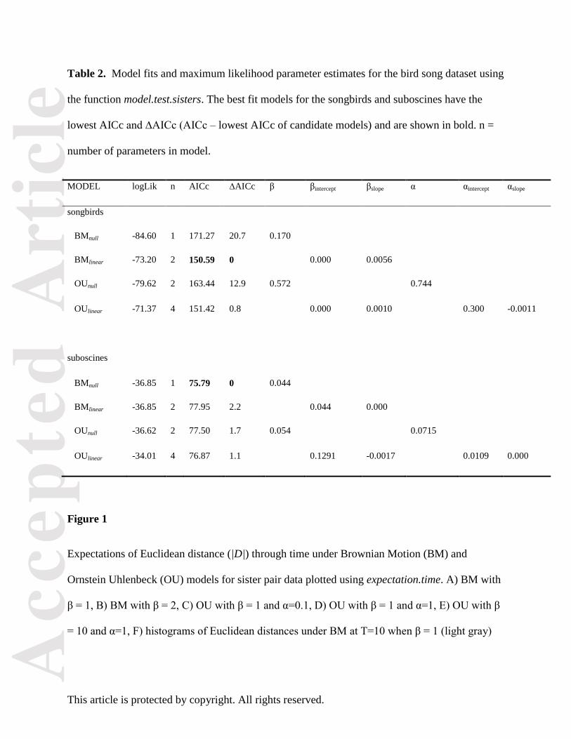
songbirds and suboscines using the BMnull models. The Akaike Information Criterion (AIC)

indicated better support (where the model with lowest AIC value is best supported) for the model

estimating separate rates for each suborder (AIC = 247.01) than for the model that estimated a

single rate across all suborders (AIC = 267.74). For this best fit model, the rate measured for

songbirds was 4 times faster than in suboscines (songbirds: β = 0.170; suboscines: β = 0.044)

leading credence to the hypothesis that learning accelerates song evolution.

However, suboscines have very low species richness at high latitudes, while songbirds

have much higher species richness there. Thus, the apparent faster rates in songbirds could be an

artefact of faster evolutionary rates at temperate versus tropical latitudes, rather than between

songbirds and suboscines. Many factors differ with latitude (e.g. migratory tendency,

paleoclimatic fluctuations, species richness, duration of the courting period) that could drive

latitudinal differences in rate. If song learning does accelerate song evolution, then we would

expect evolutionary rates to be faster in songbirds versus suboscines at all latitudes. To test this,

we included the midpoint latitude (G) of each sister pair as a continuous variable over which

rates of evolution (β) could vary. The analysis tested for latitudinal effects in songbirds and

suboscines separately and included both discrete (songbird versus suboscine) and continuous

(midpoint latitude) effects on evolutionary rates.

Acc

epte

d A

rtic

le


Adding latitude greatly improved the fit to the data (Table 2) with BMlinear best fit to the

songbird and BMnull to the suboscine subsets. 1000 simulations were used to determine the

appropriate threshold ∆AICc value necessary retain a model misspecification rate of 0.05.

Songbirds require a threshold ∆AICc value of 1.7, and suboscines a value of 1.9, which are

slightly lower than thresholds obtained for the simulated datasets used in the above analyses on

model performance. ∆AICc for the best fit gradient model versus the best fit constant rate model

in songbirds (12.9) greatly exceeded these thresholds indicating strong support for the gradient

model, while suboscines failed to support a gradient model.

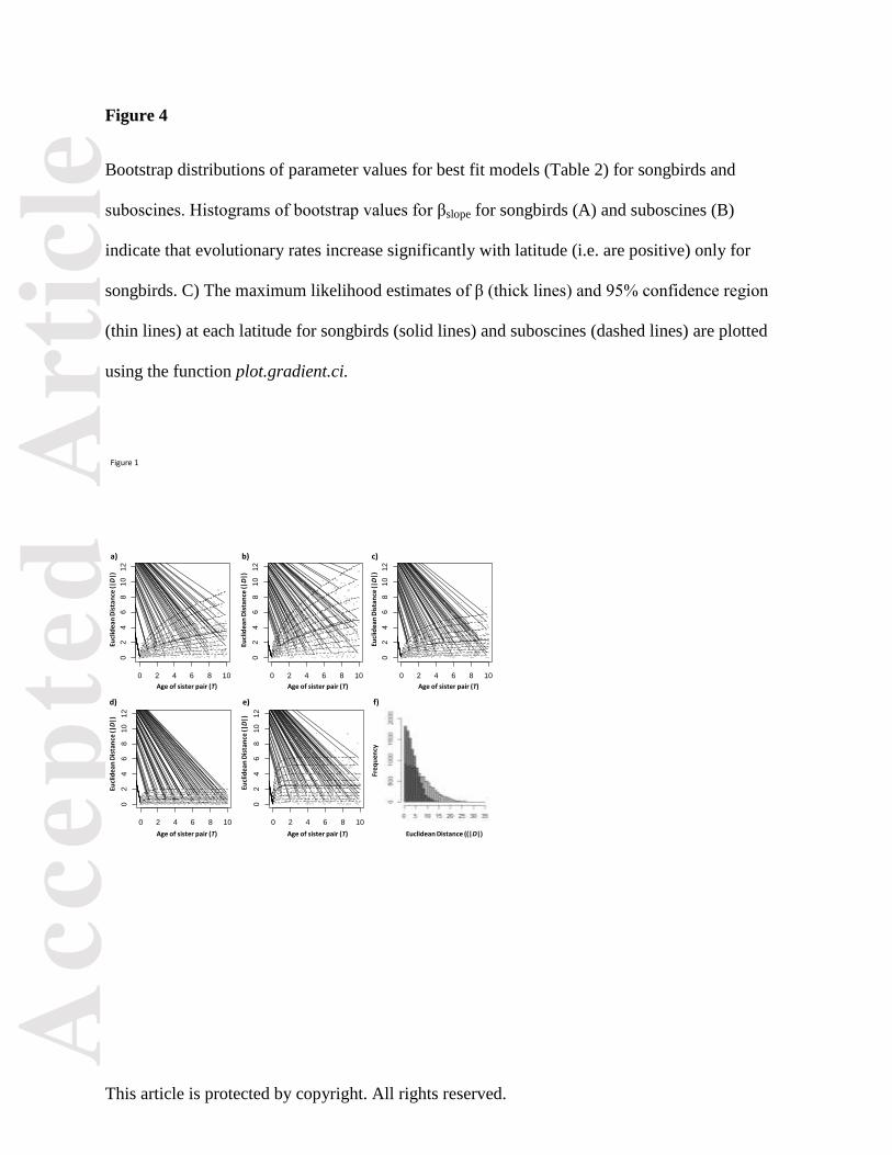
Ten thousand bootstrap replicates (using the function bootstrap.test) show the slope

parameter for β is significantly positive in songbirds, indicating an increase in evolutionary rate

with latitude (Fig. 4a). In suboscines, we also performed bootstrap replicates using BMlinear even

though BMnull had best support. The maximum likelihood estimate under BMlinear suggests rates

decline slightly with increasing latitude, though the bootstrap confidence intervals on slope

indicate that this decline is not significant (Fig. 4b), thus confirming the lack of support for a

gradient model. 95% confidence regions for evolutionary rate were calculated across the

latitudinal gradient from the bootstrap analyses (Fig. 4c).

The results show that songbirds have significantly faster evolutionary rates than

suboscines only above 15° latitude, and that rates for the two groups do not differ greatly at

tropical latitudes. Given that song learning is believed to occur in songbirds at both tropical and

temperate latitudes, these results suggest that song learning by itself cannot explain the faster

rates of syllable evolution at high latitudes. Rather, some other factor that varies with latitude

and interacts with song learning, must drive the accelerated rates in high latitude songbirds.

Sexual selection on song is one such candidate (Irwin 2000; Weir & Wheatcroft 2011). More

Acc

epte

d A

rtic

le


intense sexual selection at high latitudes (e.g. due to the short courting period, and the

importance of song during this period for mate choice) acting on cultural innovations in song

might underlie these patterns, but requires further testing. This example illustrates how an

incorrect conclusion about the positive role of song learning in accelerating evolutionary rates

would have been reached if latitude had not been accounted for in this model, because without

including latitude, songbirds appeared to have significantly faster evolutionary rates.

Summary

By allowing for both discrete and continuous effects on evolutionary rate, the modelling

framework provided in EvoRAG allows great flexibility in testing the underlying causes of trait

evolution. One disadvantage of our modelling approach is that only sister pair data are used,

which results in the exclusion of some species on a phylogeny, and does not include information

from interior portions of a phylogeny as in whole tree approaches. While these models could be

extended to whole tree approaches, doing so would require ancestor state reconstruction at

interior nodes, or other sorts of assumptions about how evolution proceeds at interior positions of

a phylogeny. Such assumptions could compromise the validity of a whole tree approach when

testing the effects of gradients. Using sister pairs provides much greater flexibility in the

modelling framework (e.g. ancestor state reconstruction is unnecessary when modelling

divergences; each sister has its own optimum under OU rather than one or a few optima as in

whole phylogeny approaches) and allows data to be easily pooled from unrelated taxonomic

groups (e.g. for which an encompassing phylogeny is not available). For these reasons, we feel

that utilization of sister pair data is an effective means of testing the effect of continuous

gradients on trait evolution.

Acc

epte

d A

rtic

le


Acknowledgements

Gavin Thomas, Trevor Price, the associate editor, and one anonymous reviewer helped to

improve this manuscript. This project was funded by a Natural Sciences and Engineering

Research Council of Canada Discovery Grant to JTW (402013-2011). Computations were

performed in part on the gpc supercomputer at the SciNet HPC Consortium. SciNet is funded by:

the Canada Foundation for Innovation under the auspices of Compute Canada, the Government

of Ontario, Ontario Research Fund - Research Excellence, and the University of Toronto.

Data Accessibility

- R scripts and example bird song dataset: available in the R package EvoRAG 2.0.

References

Baptista, L. F. (1996) Nature and its nurturing in vocal development. Ecology and evolution of

acoustic communication in birds (eds D. E. Kroodsma & E. H. Miller),pp. 39 – 60.

Cornell University Press, Ithaca, NY.

Beaulieu, J. M. & O’Meara, B. (2012) OUwie: Analysis of evolutionary rates in an OU

framework. (R package), http://CRAN.R-project.org/package=OUwie

Burnham, K. P. & Anderson, D. R. (2001) Kullback-Leibler information as a basis for strong

inference in ecological studies. Wildlife Research, 28, 111-119.

Eastman, J. M., Alfaro, M. E., Joyce, P., Hipp, A. L. & Harmon, L. J. (2011) A novel

comparative method for identifying shifts in the rate of character evolution on trees.

Evolution, 65, 3578–3589.

http://cran.r-project.org/package=OUwie

Acc

epte

d A

rtic

le


Felsenstein, J. (1973) Maximum-likelihood estimation of evolutionary trees from continuous

characters. Am. J. Hum. Genet., 25, 471-492.

Felsenstein, J. (2008) Comparative methods with sampling error and within-species variation:

contrasts revisited and revised. Am. Nat. 171, 713-725.

Fitzjohn, R. G. (2012) Diversitree: comparative phylogenetic analysis of diversification in R.

Meth. Ecol. Evol. 3, 1084-1092.

Harmon, L. J., & Losos, J. B. (2005) The effect of intraspecific sample size on type I and type II

error rates in comparative studies. Evolution, 59, 2705-2710.

Harmon, L. J., Losos, J. B., Davies, T. J., Gillespie, R. G., Gittleman, J. L., Jennings, W. B.,

Kozak, K. H., McPeek, M. A., Moreno-Roark, F., Near, T. J. et al. (2010) Early bursts of

body size and shape evolution are rare in comparative data. Evolution, 64, 2385–2396.

Harmon, L. J., Weir, J. T., Brock, C. D., Glor, R. E. & Challenger, W. (2008) GEIGER:

investigating evolutionary radiations. Bioinformatics, 24, 129–131.

Irwin, D. E. (2000) Song variation in an avian ring species. Evolution, 54, 998– 1010.

Jønsson, K. A., Fabre, P., Fritz, S. A., Etienne, R. S., Ricklefs, R. E., Jørgensen, T. B., Fjeldså,

J., Rahbek, C., Ericson, P. G. P., Woog, F., et al. (2012) Ecological and evolutionary

determinants for the adaptive radiation of the Madagascan vangas. Proceedings of the

National Academy of Sciences, USA, 109, 6620–6625.

King, A. A. & Butler, M. A. (2009) ouch: Ornstein-Uhlenbeck models for phylogenetic

comparative hypotheses (R package), http://ouch.r-forge.r-project.org

Lanfear, R., Welch, J. J., & Bromham, L. (2010) Watching the clock: Studying variation in rates

of molecular evolution between species. TREE 25, 495-503.

http://ouch.r-forge.r-project.org/

Acc

epte

d A

rtic

le


Lartillot, N., & Poujol, R. (2010) A phylogenetic model for investigating correlated evolution of

substitution rates and continuous phenotypic characters. Mol. Biol. Evol. 28, 729-744.

Lawson, A. M., &Weir, J. T. (2014) Latitudinal gradients in climatic-niche evolution accelerate

trait evolution at high latitudes. Ecology Letters. doi: 10.1111/ele.12346

O’Meara, B.C., Ané, C., Sanderson, M.J. &Wainwright, P. (2006) Testing for different rates of

continuous trait evolution using likelihood. Evolution, 60, 922–933.

Paradis, E., Claude, J. & Strimmer, K. (2004) APE: analyses of phylogenetics and evolution in R

language. Bioinformatics, 20, 289-290

Rabosky D. L. (2014) Automatic detection of key innovations, rate shifts, and diversity-

dependence on phylogenetic trees. PLOS one, 9, e89543.

Revell, L. J., Mahler, D.L., Peres-Neto, P.R., & Redelings, B.D. (2012) A new phylogenetic

method for identifying exceptional phenotypic diversification. Evolution, 66, 135-146.

Revell, L. J. (2012) phytools: An R package for phylogenetic comparative biology (and other

things). Methods Ecol. Evol., 3, 217-223.

Rowe, M., Albrecht, T., Cramer, E. R. A., Johnsen, A., Laskemoen, T., Weir, J.T., & J.T. Lifjeld.

(2015) Postcopulatory sexual selection is associated with accelerated evolution of sperm

morphology. Evolution. DOI: 10.1111/evo.12620

Seddon, N., Botero, C. A., Tobias, J. A., Dunn, P. O., MacGregor, H. E. A., Rubenstein, D. R.,

Uy, J. A. C., Weir, J. T., Whittingham, L. A., & Safran. R. J. (2013) Sexual selection

accelerates signal evolution during speciation. Proceedings of the Royal Society of

London, B, 280, 20131065.

Acc

epte

d A

rtic

le


Stack, J. C., Harmon, L. J., & O’Meara, B. (2011) RBrownie: an R package for testing

hypotheses about rates of evolutionary change. Methods in Ecology and Evolution, 2,

660–662.

Thomas, G. H. & Freckleton, R. P. (2012) MOTMOT: models of trait macroevolution on trees.

Methods in Ecology and Evolution, 3, 145–151.

Thomas, G. H., N. Cooper, C. Venditti, A. Meade, & R. P. Freckleton. (2014). Bias and

measurement error in comparative analyses: a case study with the Ornstein Uhlenbeck

model. bioRxiv http://dx.doi.org/10.1101/004036

Weir, J. T. & Wheatcroft, D. J. (2011) A latitudinal gradient in evolutionary rates of bird song

complexity and length. Proceedings of the Royal Society of London, ., 78, 1713–1720.

Weir, J. T., Wheatcroft, D. J., & Price, T. (2012) The role of ecological constraint in driving the

evolution of avian song frequency across a latitudinal gradient. Evolution, 66, 2773-2783.

Table 1 Parameter bias in models simulated under BMnull with β=0.1 and dataset size of 30 or 300 sister

pairs and fit to various test models. Median parameter values of fitted models obtained from 1000

simulations.

N Simulated Model

Test Model Bias in β_slope

Bias in α Bias in α starting

Bias in α slope

30 BMnull BMlinear 0.00002 NA NA NA

300 BMnull BMlinear 0.00004 NA NA NA

30 BMnull OUnull NA 0.01326 NA NA

300 BMnull OUnull NA 0.01073 NA NA

30 BMnull OUβ-linear -0.00005 0.01076 NA NA

300 BMnull OUβ-linear 0.00007 0.00736 NA NA

30 BMnull OUlinear 0.00003 NA 0.00000 0.00000

300 BMnull OUlinear 0.00019 NA 0.00000 0.00000

http://dx.doi.org/10.1101/004036

Acc

epte

d A

rtic

le


Table 2. Model fits and maximum likelihood parameter estimates for the bird song dataset using

the function model.test.sisters. The best fit models for the songbirds and suboscines have the

lowest AICc and ∆AICc (AICc – lowest AICc of candidate models) and are shown in bold. n =

number of parameters in model.

MODEL logLik n AICc ∆AICc β βintercept βslope α αintercept αslope

songbirds

BMnull -84.60 1 171.27 20.7 0.170

BMlinear -73.20 2 150.59 0 0.000 0.0056

OUnull -79.62 2 163.44 12.9 0.572 0.744

OUlinear -71.37 4 151.42 0.8 0.000 0.0010 0.300 -0.0011

suboscines

BMnull -36.85 1 75.79 0 0.044

BMlinear -36.85 2 77.95 2.2 0.044 0.000

OUnull -36.62 2 77.50 1.7 0.054 0.0715

OUlinear -34.01 4 76.87 1.1 0.1291 -0.0017 0.0109 0.000

Figure 1

Expectations of Euclidean distance (|D|) through time under Brownian Motion (BM) and

Ornstein Uhlenbeck (OU) models for sister pair data plotted using expectation.time. A) BM with

β = 1, B) BM with β = 2, C) OU with β = 1 and α=0.1, D) OU with β = 1 and α=1, E) OU with β

= 10 and α=1, F) histograms of Euclidean distances under BM at T=10 when β = 1 (light gray)

Acc

epte

d A

rtic

le


and β = 4 (dark gray). Solid lines indicate mean and dashed lines from bottom to top indicate the

percentiles 10, 20…90, 95.

Figure 2

Accuracy of parameter estimation in EvoRAG assessed through simulation for the BMlinear and

OUlinear models. Dashed lines show the simulated model parameter. Median values and

interquartile ranges are plotted for datasets of 30 to 300 sister pairs.

Figure 3

Rates of model misspecification as a function of the number of sister pairs. A) Proportion of

constant rate simulations (BM: black circles β=0.1; gray circles β=1. OU: black triangles β=0.1,

α = 0.05; gray circles β=0.1, α=2) for which AICc favored a rate variable model. B) Threshold

∆AICcCR scores necessary to maintain an error rate of 0.05 for BM (black circles β=0.1; gray

circles β=1) and OU (black triangles β=0.1, α = 0.05; gray circles β=0.1, α=2). C) Proportion of

rate variable simulations under BMlinear for which AICc favored a rate constant model when β

increases 2 (palest gray), 3 (pale gray), 4 (medium gray), 6 (dark gray), and 10 (black) fold over

the gradient. D) proportion of 4000 rate variable simulations under OUlinear for which AICc

favored a rate constant model under four scenarios: 1) β increases 2-fold and α declines 2-fold

(palest gray), 2) β increases 2-fold and α declines 4-fold (pale gray), 3) β increases 4-fold and α

declines 2-fold (dark gray), and 4) β increases 4-fold and α declines 4-fold (black), from starting

values of β = 0.1 and α = 0.8.

Acc

epte

d A

rtic

le


Figure 4

Bootstrap distributions of parameter values for best fit models (Table 2) for songbirds and

suboscines. Histograms of bootstrap values for βslope for songbirds (A) and suboscines (B)

indicate that evolutionary rates increase significantly with latitude (i.e. are positive) only for

songbirds. C) The maximum likelihood estimates of β (thick lines) and 95% confidence region

(thin lines) at each latitude for songbirds (solid lines) and suboscines (dashed lines) are plotted

using the function plot.gradient.ci.

Figure 1

0 2 4 6 8 10

02

46

81

01

2

Genetic distance of sister pair

Eu

clid

ea

n d

ista

nce

0 2 4 6 8 10

02

46

81

01

2


Eu

clid

ea

n d

ista

nce

0 2 4 6 8 10

02

46

81

01

2


Eu

clid

ea

n d

ista

nce

0 2 4 6 8 10

02

46

81

01

2


Eu

clid

ea

n d

ista

nce

0 2 4 6 8 10

02

46

81

01

2


Eu

clid

ea

n d

ista

nce

Eucl

idea

n D

ista

nce

(|D

|)

Euclidean Distance ((|D|)

Eucl

idea

n D

ista

nce

(|D

|)

Eucl

idea

n D

ista

nce

(|D

|)Eu

clid

ean

Dis

tan

ce (|D

|)

Eucl

idea

n D

ista

nce

(|D

|)Fr

eq

uen

cy

a) b)

Age of sister pair (T) Age of sister pair (T) Age of sister pair (T)

Age of sister pair (T)Age of sister pair (T)

c)

d) e) f)

Acc

epte

d A

rtic

le


0.00

0.05

0.10

0.15

0.20

0.25

0.30

1 2 3 4 5 6

0.00

0.02

0.04

0.06

0.08

0.10

0.12

0.14

1 2 3 4 5 6

0.0000

0.0005

0.0010

0.0015

0.0020

0.0025

0.0030

1 2 3 4 5 6

0.0

0.5

1.0

1.5

2.0

2.5

3.0

1 2 3 4 5 6

-0.030

-0.025

-0.020

-0.015

-0.010

-0.005

0.000

0.005

1 2 3 4 5 6

0.000

0.001

0.002

0.003

0.004

0.005

1 2 3 4 5 6

Number of sister pairs

30 60 90

120

150

300

30 60 90

120

150

300

30 60 90 120

150

300

30 60 90

120

150

300

30 60 90

120

150

30030 60 90

120

150

300


βst

arti

ng

βsl

op

eβ

slo

pe

βst

arti

ng

αst

arti

ng

αsl

op

e

BMlinear BMlinear

OUlinearOUlinear

OUlinearOUlinear

Acc

epte

d A

rtic

le



Pro

po

rtio

n m

issp

ecif

ied

a)

c)

b)

Pro

po

rtio

n m

issp

ecif

ied

Pro

po

rtio

n m

issp

ecif

ied

0

1

2

3

4

5

0

50 100

150

200

250

300

Thre

sho

ld ∆

AIC

c

d)

Acc

epte

d A

rtic

le


Fre

qu

ency

Fre

qu

ency

a)

βslope βslope Absolute latitude

c)

Evo

luti

on

ary

rate

(β)

0 10 20 30 40 50 60

0.0

0.1

0.2

0.3

0.4

0.5

Latitude

Evo

lutio

na

ry R

ate

b)

Documents

olutionary Rates Across Gradients