Embed Size (px)
Citation preview

Finn Roar Aune, Torstein Bye ,
Tor Amt Johnsen and Alexandra Katz
96/19 September 1996 Documents
Statistics NorwayResearch Department
NORMENA General Equilibrium Model of theNordic Countries Featuring a DetailedElectricity Block

Documents 96/19 • Statistics Norway, September 1996
Finn Roar Aune, Torstein Bye,Tor Amt Johnsen and Alexandra Katz
NORMENA General Equilibrium Model of theNordic Countries Featuring a DetailedElectricity Block
AbstractThis paper presents a Nordic energy market model, NORMEN, which links together the electricitymarket, the economy and the environment in a general equilibrium framework. The model is anextension of an earlier partial energy market model developed at Statistics Norway. In contrast to thatand other partial models (i.e. the bulk of the literature) where there are no feedback effects from theelectricity prices to the rest of the economy, in NORMEN all prices are determined simultaneously. Byadding a macroeconomic block to the model, the scale effects on electricity demand due to electricityprice changes can be captured, rather than just first round price effects. In this paper, we document themodel structure of NORMEN, parameter estimation procedures, and data collecting process. Thisdocument marks the end of the first stage of this project: model building and data collecting. In thenext stage, we will use the model, among other things, to analyze the effect of various energy policieson electricity consumption, electricity prices, CO2 emissions, and several general economic indicators.
Keywords: Electricity demand, computable general equilibrium models, energy policy analysis
JEL classification: El 0, F47, Q43
Acknowledgement: Financial support from The Research Council of Norway for the development ofthe model is gratefully acknowledged.
Address: Finn Roar Aune, Statistics Norway, Research Department,P.O.Box 8131 Dep., N-0033 Oslo, Norway. E-mail: [email protected]
Torstein Bye, Statistics Norway, Research Department, E-mail: [email protected]
Tor Arnt Johnsen, Statistics Norway, Research Department, E-mail: [email protected]
Alexandra Katz, Statistics Norway, Research Department, E-mail: [email protected]


1. IntroductionOver the last few years, electricity industries the world over have come under increasing pressure to
deregulate. This is partly due to the realization that vertically integrated electricity monopolies have
been inefficient and that welfare gains could be realized by opening up electricity systems to
competition. Furthermore, several countries have already begun the liberalization process with
relative success. The UK in 1990 was the first European country to begin liberalizing its electricity
supply industry (ESI) and Norway the second a year later. Because Sweden has recently followed suit
and Finland is not long behind, a common deregulated Nordic electricity market is now almost a
reality. Together, Norway, Sweden, and Finland account for about 90% of Nordic power generation,
so even though Denmark will probably not deregulate for some time, the Nordic electricity market can
still be basically characterized as open. Since there are large variations across countries in power
generation methods and thus in cost structures, there may be substantial returns to Nordic trade in
electricity.
A partial energy market model for the Nordic countries was developed a few years ago at Statistics
Norway in order to analyze the supply and demand for energy in four countries: Norway, Sweden,
Denmark, and Finland. The Nordic energy market model considered the final demand and supply for
fuel oil and electricity using water, gas, oil, coal, uranium, and biofuels as inputs in electricity
production. It was used to analyze the effects of establishing a Nordic energy market and to test the
response of energy demand to various scenarios of CO 2 taxes, see Bye et al. (1995), Bye and Johnsen
(1995), and Aune et al. (1995). However, the model relied on exogenous economic activity levels and
prices.
A new and extended version of the Nordic energy market model is presented in this paper. The model
is innovative in that it is a general equilibrium model featuring a detailed electricity block, combined
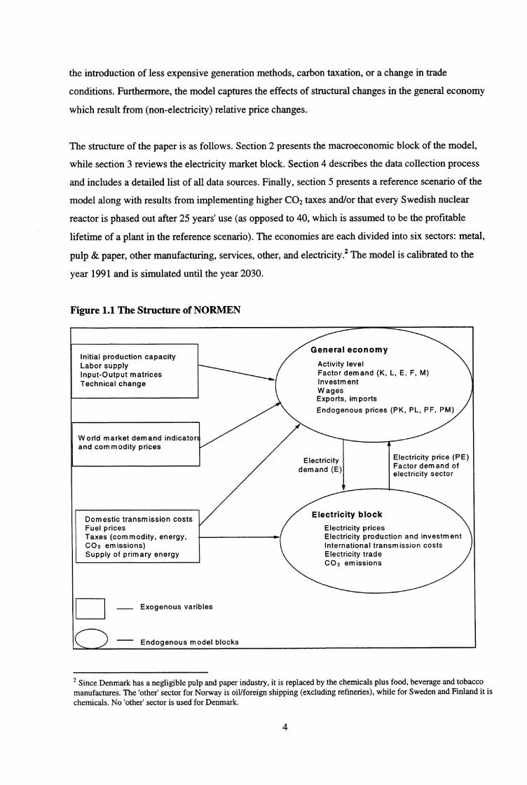
with trade of electricity between countries. As figure 1.1 shows, the new general economy blocks
determine the activity levels of the Nordic economies (GDP) and are linked to the (old) electricity
block of the model. Whereas before there were no feedback effects from the electricity prices to the
general economy, in NORMEN 1 all domestic prices (of electricity and other goods) are determined
simultaneously. Such a linkage is important because electricity prices differ widely among countries
as well as for various domestic end-uses. By using a model where the electricity market and general
economy are connected, scale effects on electricity demand due to electricity price changes can be
captured, rather than just first round price effects. Such price changes might result, for example, from
1 NORdic Macro ENergy market model
3
General economy
Activity levelFactor demand (K, L, E, F, M)InvestmentWagesExports, imports
Endogenous prices (PK, PL, PF, PM)
CD
the introduction of less expensive generation methods, carbon taxation, or a change in trade
conditions. Furthermore, the model captures the effects of structural changes in the general economy
which result from (non-electricity) relative price changes.
The structure of the paper is as follows. Section 2 presents the macroeconomic block of the model,
while section 3 reviews the electricity market block. Section 4 describes the data collection process
and includes a detailed list of all data sources. Finally, section 5 presents a reference scenario of the
model along with results from implementing higher CO 2 taxes and/or that every Swedish nuclear
reactor is phased out after 25 years' use (as opposed to 40, which is assumed to be the profitable
lifetime of a plant in the reference scenario). The economies are each divided into six sectors: metal,
pulp & paper, other manufacturing, services, other, and electricity. 2 The model is calibrated to the
year 1991 and is simulated until the year 2030.
Figure 1.1 The Structure of NORMEN
Initial production capacityLabor supplyInput-Output matricesTechnical change
World market demand indicatorand commodity prices
Electricitydemand (E)
Electricity price (PE)Factor demand ofelectricity sector
Electricity block
Electricity pricesElectricity production and investmentInternational transmission costsElectricity tradeCO2 emissions
Dom estic transmission costsFuel pricesTaxes (commodity, energy,CO2 emissions)Supply of primary energy
Exogenous varibles
Endogenous model blocks
2 Since Denmark has a negligible pulp and paper industry, it is replaced by the chemicals plus food, beverage and tobaccomanufactures. The 'other' sector for Norway is oil/foreign shipping (excluding refineries), while for Sweden and Finland it ischemicals. No 'other' sector is used for Denmark.
4

2. The Macroeconomic Block
2.1. Production and Factor Demand EquationsProduction in sector j, (Xj), is defined as a Cobb-Douglas function of the five inputs (xn), where n
electricity (E), fuel oil (F), capital (K), labor (L), and other material inputs (M) for each Nordic
country. 3
(1) =Ain X ccniP j , n=E,F,K,L,M;Vj# 6
where anj and A; are coefficients and a„j>0. The assumption of constant returns to scale implies
(2) anj= 1 . n=E,F,K,L,M; Vj# 6
Assuming cost minimizing behavior, deriving the first order conditions and combining them with the
primal function yields the dual cost function, see Varian (1978),
(3) c(p,x; ) = aanini )-1(ri PiCii nin n
where p is the vector of input prices. Applying Shephard's lemma (i.e. taking the first order
derivatives of the cost function with respect to input price) yields the conditional factor demand
function'', and thus the unit input demand coefficient for factor n in sector j can be expressed as
(4) z nj = a janynli n=E,F,K,L,M;Vj#6
where
a.= (A • riaay,i) --, j nj
The coefficient Aj then calibrates the model.
3 The country index is omitted for ease of presentation. Electricity (sector j=6) is treated separately in Section 3.4 When calibrating the input demand functions, there is an exact identity between the coefficients in these functions and theprimal function.
(5)
5
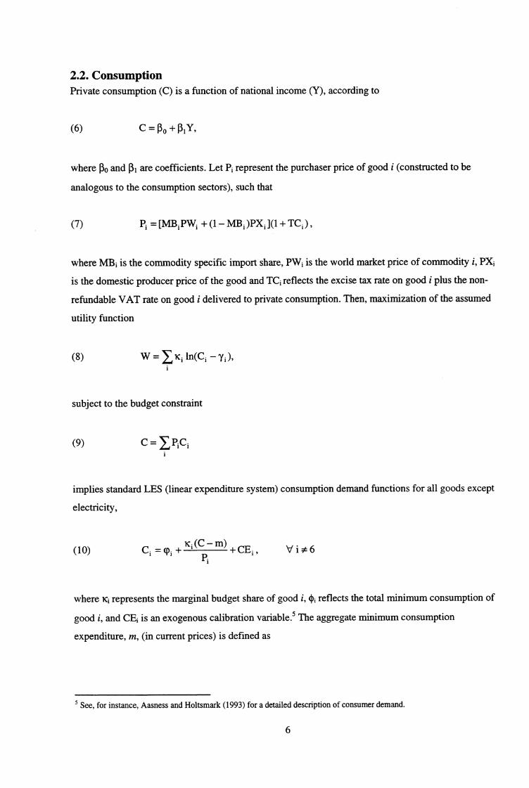
2.2. ConsumptionPrivate consumption (C) is a function of national income (Y), according to
(6) C = po +
where po and p i are coefficients. Let P i represent the purchaser price of good i (constructed to be
analogous to the consumption sectors), such that
(7) Pi = [MB i PWi + (1— MB, )PX i ](1 + TC i ) ,
where MBi is the commodity specific import share, PW i is the world market price of commodity i, PXi
is the domestic producer price of the good and TC i reflects the excise tax rate on good i plus the non-
refundable VAT rate on good i delivered to private consumption. Then, maximization of the assumed
utility function
(8) W = K i ln(C i — y i ),
subject to the budget constraint
(9) C PiC i
implies standard LES (linear expenditure system) consumption demand functions for all goods except
electricity,
(10)Ki —
C i = Ti + +CEi, Vi#6Pi
where lq represents the marginal budget share of good i, (1)i reflects the total minimum consumption of
good i, and CEi is an exogenous calibration variable. 5 The aggregate minimum consumption
expenditure, m, (in current prices) is defined as
5 See, for instance, Aasness and Holtsmark (1993) for a detailed description of consumer demand.
6

The marginal budget share estimates used are reported in table 2.1. For Norway, the 1991 (base year)
shares are derived from estimates from Aasness and Holtsmark (1993). For Sweden, they come from
the National Institute of Economic Research (1996) and are based on the average of the period 1970-
1992 (1985 base year). The Danish shares are based on the 1990 consumption parameters estimated
for their GESMEC mode1. 6 Unfortunately, no recent marginal budget shares for Finland have been
found, and therefore they are temporarily 'guesstimated' by the Norwegian ones.
Table 2.1 Consumption parameter estimate?
Sector
Norwegian marginal
budget shares,
1991
Swedish marginal
budget shares,
avg. 1970-1992
Danish marginal
budget shares,
1990
Finnish marginal
budget shares,
1991*
Metal .06b
P & P .06c
Other Industries .281 .340 .14 .281
Services .719 .660 .73 .719
Other
Electricity
a Note that since metal, pulp and paper, chemicals and oil/ocean transport (in 'Other') are not consumer goods, they are notrelevant here. Electricity consumption is determined in the electricity block.b NB electricity-intensive industries
NB food productsSources: Norway: Aasness and Holtsmark (1993); Sweden: National Institute of Economic Research (1996); Denmark:derived from Danish Economic Council (1995a); *Finland: temporarily 'guesstimated' by Norwegian shares.
2.3. InvestmentCapital input is determined by the production functions and gross investment by equation (12). That
is, we assume that gross investment, has full capacity effect the same period that investment takes
place,
(12) • = • + • —.1 it Kit D it K
where Di is depreciation calculated according to
6 See Danish Economic Council (1995a).
7

(13) Dit = 5 iKyt-0
and where the depreciation rate, 8j , is determined in the base year. The electricity generating sector is
treated in a bit more detail. Summing over the K different electricity production technologies yields
total new investment in that sector
(14) Jjt = Dkjt - j= 6 (el.);k= 1, 2,...K
k
The K possible technologies are: condensing generation (coal fired), coal dust, coal-gas, coal-fired
fluid bed, condensing generation (oil-fired), back pressure, gas turbine (new), combined cycle (gas)
based on either national sources' or Norwegian tradable Troll gas/tradable Halten gas, wood-fired
steam injected gas cycle (STIG), condensing generation (peat-fired), condensing generation (biofuel-
fired), and new hydropower (only for Norway, and consisting of four different types according to
development costs).
2.4. Foreign TradeIn accordance with the Armington hypothesis, which states that domestic and foreign goods are
imperfect substitutes, exports of commodity i (XPi) for each country depend on the domestic
purchaser price (PX1) relative to the world market price of the good (PW) and on the world market
demand indicator for the commodity (MI). Accordingly, exports to the rest of the world are
represented as
(15)PX
xPi = )EP' MI ennPW,
i*6
where co and F..mi are the relative price and market elasticities, respectively, and Xo is a calibration
parameter. Table 2.2 presents the export elasticities implemented in the model.
7 A national source is an exogenously limited supply of natural gas which is allocated to just one country. (Russian gas toFinland. Danish gas to Denmark and Sweden.)
8
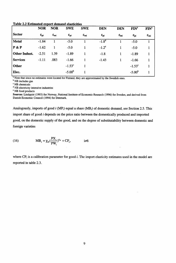
Table 2.2 Estimated export demand elasticitiesNOR NOR SWE SWE DEN DEN
FINS
Sector Epj EMi Epi Erni Epi Erni
Emi
Metal -1.84 1 -5.0 1 -1.8d 1 -5.0 1
P& P -1.62 1 -5.0 1 -1.2e 1 -5.0 1
Other Indust. -2.51 1.39 -1.89 1 -1.8 1 -1.89 1
Services -1.11 .083 -1.66 1 -1.43 1 -1.66 1
Other -1.53c 1 -1.53c 1
Elec. -5.00b 1 _5.00b 1
a Note that since no estimates were located for Finland, they are approximated by the Swedish ones.b NB includes gas
NB chemicalsd NB electricity intensive industriese NB food productsSources: Lindquist (1993) for Norway, National Institute of Economic Research (1996) for Sweden, and derived fromDanish Economic Council (1994) for Denmark.
Analogously, imports of good i (MPi) equal a share (MB i) of domestic demand, see Section 2.5. This
import share of good i depends on the price ratio between the domestically produced and imported
good, on the domestic supply of the good, and on the degree of substitutability between domestic and
foreign varieties
(16)PX
MB, = xoe-Lf1 + CPi , i#6
where CPi is a calibration parameter for good i. The import elasticity estimates used in the model are
reported in table 2.3.
9

Table 2.3 Estimated import elasticities
Sector
NOR
Esi
SWE
Esi
DEN
ESi
FINa
ESi
Metal .81 1.1 1.2d 0.8
P & P 2.35 1.1 .9e 2.3
Other Industries 2.51 .8 1.2 1.3
Services 1.11 1.01 1.43 1.2
Other - 0.8c 1.0c
Electricity - Ob - Ob
a Note that since no estimates were located for Finland, they are 'guestimated' by a combination of the Swedish andNorwegian ones.b NB includes gas
NB chemicalsd NB electricity intensive industriese NB food productsSources: Naug (1994) for Norway, National Institute of Economic Research (1996) for Sweden, andDanish Economic Council (1994) for Denmark.
2.5. Commodity Market EquilibriumImports of good i equal a share (MB ;) of domestic demand for each good. Total supply of commodity
i in each country must equal total domestic usage of the good plus exports and a correction term, nio
(determined in the base year). Note that the model has a single product production structure, such that
i=j and that electricity and fuels are treated in detail in Section 3.
MPi = MB i [IQVI j + +Ci +G i +DL i ] Vi#6
(17) X i = +Ci +G i +DLJ+XPi + a io di 6
X i E + MP E = +Gi +)(P E i = 6 (el.); Vj
X i F + MP F = +Gi +)(P F i = 6 (fuel. ); Vj
That is, output of good i (basic value) equals the sum of deliveries of good i to intermediate
production, to investment, to private consumption C i (basic value), to public consumption G i (basic
value), to changes in stocks (basic value) DL i, and to exports XPi, plus the correction term. The
coefficients 4, and Ili from the input-output matrices convert purchasers' values (M ai and J.) to basic
values. They are calculated, respectively, as
10

4i; = deliveries of good i to intermediate inputs in sector j (basic value) divided by the
total value of intermediate inputs to sector j (net (refundable VAT) purchaser prices in
the base year)
= the ratio of deliveries of good i (basic value) for investment to the total value of
investment in sector j (purchaser prices in the base year)
2.6. PricesIn the long run, domestic producer prices must equal total unit cost, i.e. there are no incentives for any
firms to enter or exit the market. Total unit cost in sector j is defined by
(18) PXj = IPn j Zn i +(-74(i i ), n=E,F,K,L,M;Vj
where TIA is net sectoral taxes in production sector j. The purchaser price (net refundable VAT) for
intermediate inputs other than electricity and fuel in sector j is determined according to
(19) PMT = (1 + Tij ) 4 ii [MB i PWi + (1— MBOI)X i ,
where Tij is a composite tax rate which accounts for the taxes on deliveries of good i to sector j (i.e. it
includes the rate of non-refundable VAT and the rate of excise tax on good i delivered to intermediate
inputs in sector j).
The domestic purchaser price (end-use price) of electricity in a sector (PE A)8 depends on the c.i.f.
import price of electricity (PEcif), the margin which covers transmission and distribution costs (MG JE),
the net tax on electricity used by sector j (TE;), and the value added tax rate on electricity usage
(VAT).
(20) PEA = (PEcif + MGE + TE j )(1+ VAT).
8 A detailed description of energy price determination is presented in Bye et al. (1995).
11
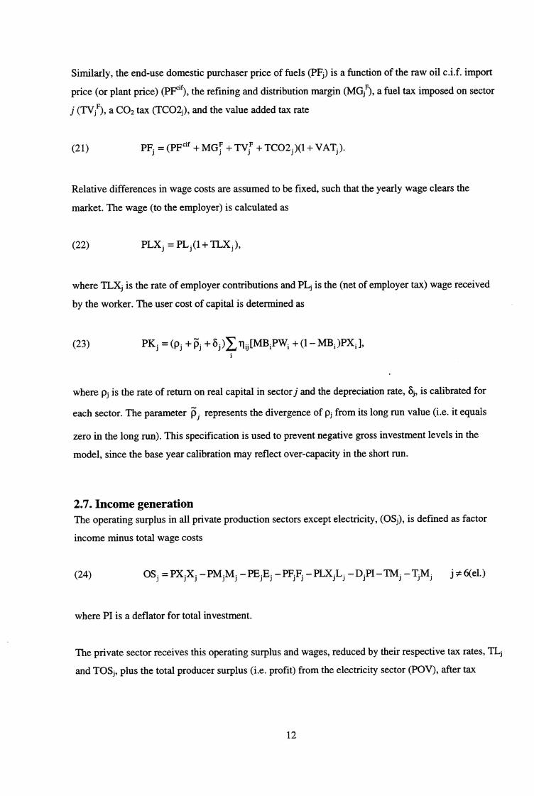
Similarly, the end-use domestic purchaser price of fuels (PF i) is a function of the raw oil c.i.f. import
price (or plant price) (13Fcif.), the refining and distribution margin (MG iF), a fuel tax imposed on sector
j (TViF), a CO2 tax (TCO2j), and the value added tax rate
(21) PFD = (PF cif + MG. + TViF + TCO2 )(1 + VAT).
Relative differences in wage costs are assumed to be fixed, such that the yearly wage clears the
market. The wage (to the employer) is calculated as
(22) PLXj = PL i (1+ TLX i ),
where TLXi is the rate of employer contributions and PL C is the (net of employer tax) wage received
by the worker. The user cost of capital is determined as
(23) PKi = (p i +13i + (1 — MBOPXJ,
where pj is the rate of return on real capital in sector j and the depreciation rate, 8j , is calibrated for
each sector. The parameter 13 i represents the divergence of p i from its long run value (i.e. it equals
zero in the long run). This specification is used to prevent negative gross investment levels in the
model, since the base year calibration may reflect over-capacity in the short run.
2.7. Income generationThe operating surplus in all private production sectors except electricity, (OS;), is defined as factor
income minus total wage costs
(24) OSi = PXiXi —PM iMi —PEiEj —PFiFj —PLXiL j —DPI—TMj —TiMi j * 6(el.)
where PI is a deflator for total investment.
The private sector receives this operating surplus and wages, reduced by their respective tax rates, TL,
and TOSS , plus the total producer surplus (i.e. profit) from the electricity sector (POV), after tax
12

(25) YP = [OS i (1 — TOS i ) + PL (1 — TL j )1+ POV(1 TPOV),j*5
where POV is defined as the market value of electricity sales minus the area under the long-run
marginal cost curve (C(u))
(26) POV = 1,[(PE)SE k — J C(u)du]'SEk
k 0
and where SEk is the total domestic quantity of electricity supplied using technology k.
The income received by the government (Y G), thus equals the sum of income taxes, operating surplus
taxes, commodity taxes (including taxes on electricity and fuel oil in the traditional production
sectors), production taxes, taxes on fuel use in the electricity generation sector, consumption taxes,
and value added taxes on oil and electricity which are paid by households
(27)
YG = PLiLi Crla j/ (OS j TOSi)+POV(TPOV) + + TiiMj*5 i j
Tiqj t„ikUink TCiCi + (WiFFi + TCO2r. Fi + Th iE j )j m k i*5
+ [(PFjcif + MGr + TVJF + TCO2 )Fj + (PE7if + MGE + TE )E i ]VAT}J
where tmk and Umk are, respectively, the tax rate for and use of energy good m, using electricity
production technology k (m includes electricity, oil, gas, coal, etc.).
2.8. The Trade BalanceThe trade balance (H) for each country depends on net exports of the 5 commodities plus net energy
exports (see Section 3)
(28) H = J (X P i — MP i ) + (XP: —i* 6
13

3. Electricity Market Block
3.1. Electricity Supply
Short runAt the starting point of the model, energy production capacity is larger than demand in the various
countries. All of the Nordic countries have had regulated energy markets. Expansion is undertaken to
ensure that demand can be met, plus a security margin. Some of the existing capacity is first put into
use when demand increases. Due to the long lifetime of the existing capacity, it can take a long time
for the new capacity to expand. Therefore, both short and long run cost functions are specified in the
model. By short run, it is meant the time horizon until the expansion of new capacity becomes
profitable.
In the short run, the maximum energy production capacity is given. Capacity data (KAP k) are
calculated for the model's first year (1991) for all of the electricity production technologies (k) which
are specified, see Section 2.3. Available energy production capacity in a country equals the sum over
all of the capacities for the K different technologies
(29)
KAP = KAPk k= 1, . K
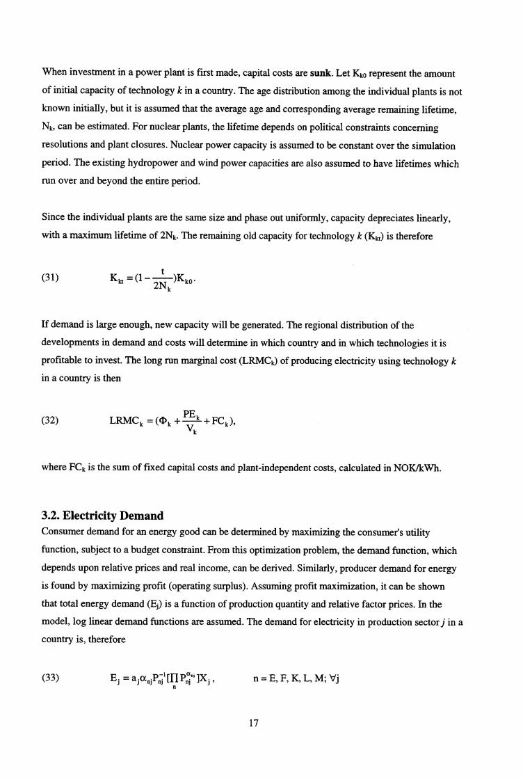
The short run supply of electricity is ranked according to rising variable costs. The fuel efficiency of
technology k, Vk, reflects the relation between the amount of energy in the form of electricity which is
produced by the supplied fuel and the theoretical energy content as a whole. For example, an energy
unit of coal supplied to a conventional coal-using plant yields .35 energy units of electricity. The rest
of the energy is lost in the combustion process in the form of heat. The variable cost (CV k) for an
energy production technology is constant when the price of supplied energy, Pk, is given
(30) CVk = (43 k +,Vk
k = 1, . K
where (13k represents the part of operating costs (in excess of energy costs) which depend upon
production. Since we do not have data for this, the operating costs are included in the fixed costs and
are assumed to be independent of production for as long as the plant operates.
14

Long runIf the market price of electricity at a power plant exceeds the long run marginal cost, defined as the
sum of fixed and variable costs of new operations (calculated per kWh per year), then there will be
investment in new capacity.
It is assumed that no electricity producer has enough power to influence the market, and thus that
there can be no monopolies in electricity trading. It is also assumed that the capacity of a power plant
can grow continuously. Since every individual plant is small relative to the total market, and since
there is also significant flexibility with regard to the scale of heating power plants, this is a reasonable
assumption.
The available heating technology is comprised partly of internationally proven technologies like oil or
coal-fired condensing generation and gas-fired combined cycle power, and partly of more country-
specific technologies like peat-fired (condense) plants in Finland, industrial combined heat and power
(CHP) in Finland and Sweden, and straw-fired CHP in Denmark. A new type of gas fired technology
(fuel cell) is also currently under development in Denmark. These types of processes have future
potential due to their high fuel efficiencies, but for now the costs are too high for such technologies to
be commercially profitable.
Data on fixed unit costs for new electricity technologies are shown below in table 3.1. Starting with
investment costs for effective capacity (per MW), data on the total hours of plant operation per year, a
discount rate of 7% and a given capital lifetime, fixed capital costs per kWh, or the user price of
energy capital, can be calculated. In addition to fixed capital costs, there are also operating costs
which depend on production. These are included in the Table 4 data. In order that the costs are
comparable, each established plant is assumed to operate 5100 hours per year. This corresponds to
about the average use time for the sum of industrial and ordinary consumption.
15
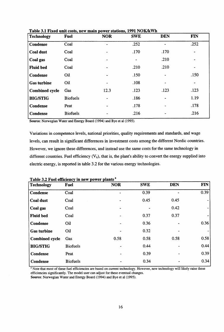
Table 3.1 Fixed unit costs, new main power stations, 1991 NOK/kWhTechnology Fuel NOR SWE DEN FIN
Condense Coal
Coal dust Coal
Coal gas Coal
Fluid bed Coal
Condense Oil
Gas turbine Oil
Combined cycle Gas
BIG/STIG Biofuels
Condense Peat
Condense Biofuels
12.3
.252 -
.170 .170
.210
.210 .210
.150 -
.108 -
.123 .123
.186 -
.178 -
.216
.252
.150
.123
1.19
.178
.216
Source: Norwegian Water and Energy Board (1994) and Bye et al (1995).
Variations in competence levels, national priorities, quality requirements and standards, and wage
levels, can result in significant differences in investment costs among the different Nordic countries.
However, we ignore these differences, and instead use the same costs for the same technology in
different countries. Fuel efficiency (VI), that is, the plant's ability to convert the energy supplied into
electric energy, is reported in table 3.2 for the various energy technologies.
Table 3.2 Fuel efficiency in new power plantsTechnology Fuel NOR SWE DEN FIN
Condense Coal
Coal dust Coal
Coal gas Coal
Fluid bed Coal
Condense Oil
Gas turbine Oil
Combined cycle Gas
BIG/STIG Biofuels
Condense Peat
Condense Biofuels
0.58
0.39 -
0.45 0.45
0.42
0.37 0.37
0.36 -
0.32 -
0.58 0.58
0.44
0.39 -
0.34
0.39
0.36
0.58
0.44
0.39
0.34
a Note that most of these fuel efficiencies are based on current technology. However, new technology will likely raise theseefficiencies significantly. The model user can adjust for these eventual changes.Source: Norwegian Water and Energy Board (1994) and Bye et al (1995).
16
When investment in a power plant is first made, capital costs are sunk. Let Kko represent the amount
of initial capacity of technology k in a country. The age distribution among the individual plants is not
known initially, but it is assumed that the average age and corresponding average remaining lifetime,
Nk, can be estimated. For nuclear plants, the lifetime depends on political constraints concerning
resolutions and plant closures. Nuclear power capacity is assumed to be constant over the simulation
period. The existing hydropower and wind power capacities are also assumed to have lifetimes which
run over and beyond the entire period.
Since the individual plants are the same size and phase out uniformly, capacity depreciates linearly,
with a maximum lifetime of 2Nk. The remaining old capacity for technology k (Kkt) is therefore
(31) Kkt (1 2Nt k )1(k°.
If demand is large enough, new capacity will be generated. The regional distribution of the
developments in demand and costs will determine in which country and in which technologies it is
profitable to invest. The long run marginal cost (LRMC k) of producing electricity using technology k
in a country is then
(32) PELRMC k = (43k -I- v + FCk ),
kk
where FCk is the sum of fixed capital costs and plant-independent costs, calculated in NOK/kWh.
3.2. Electricity DemandConsumer demand for an energy good can be determined by maximizing the consumer's utility
function, subject to a budget constraint. From this optimization problem, the demand function, which
depends upon relative prices and real income, can be derived. Similarly, producer demand for energy
is found by maximizing profit (operating surplus). Assuming profit maximization, it can be shown
that total energy demand (Es) is a function of production quantity and relative factor prices. In the
model, log linear demand functions are assumed. The demand for electricity in production sector j in a
country is, therefore
(33) E = .P7 1 [11 Pa."' PC .nj nj nj j 7n= E, F, K, L, M; Vj
17

where, recall, Xi stands for the production level in sector j, as is a constant, and where an, are the price
elasticities.
In the present model version, only two energy goods are specified, heating oil and electricity. We
have not yet succeeded in estimating substitution between other energy goods. It may be possible later
to include in the model district heating and natural gas as independent energy goods for end-use. The
data used in the model are updated to 1991, and all prices are in constant 1991 prices. Data for
household demand, purchaser (end-use) prices, total consumption, and the estimated elasticities are
used to calibrate the constant (a) which appears in the electricity demand function. The household
sector is modeled as in the partial model.
4. Data Requirements
The old version of the Nordic model contains electricity and fuel oil demand levels, energy prices and
a detailed description of electricity production (including inputs of fuel oil, electricity, coal, biofuels,
uranium, etc.), transmission and trade. For this extended model, we needed to build an extensive
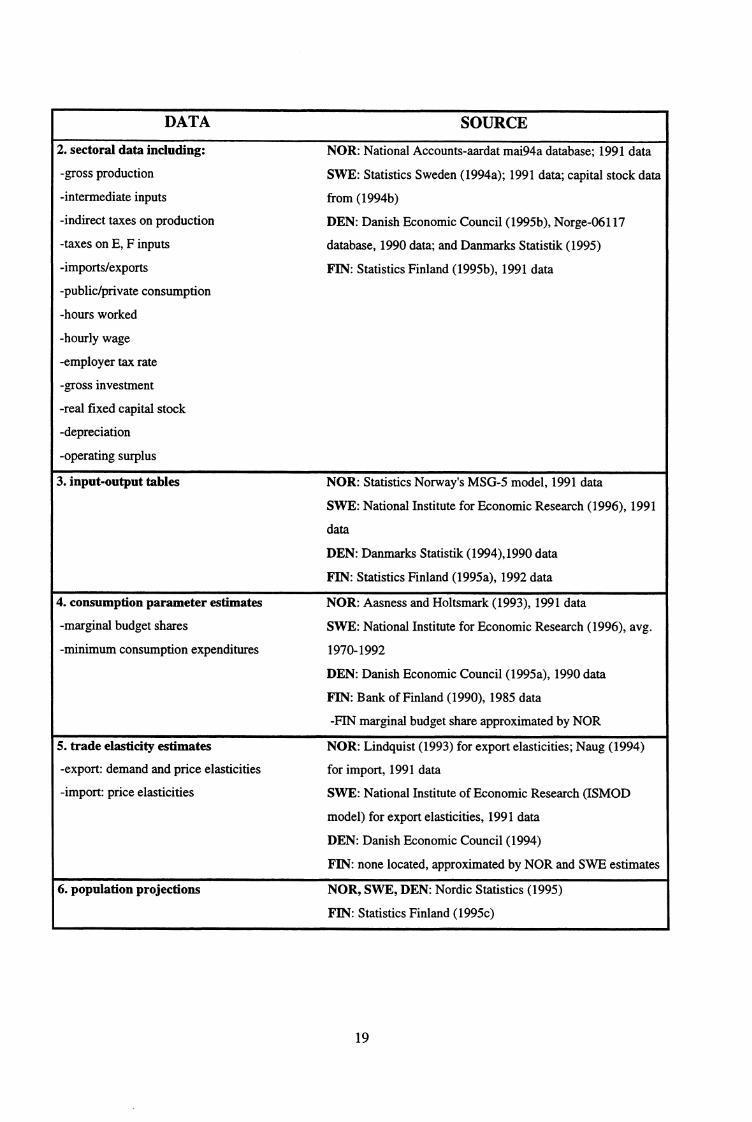
database (six sector aggregation) for each Nordic country in the base year (1991). Table 4.1 lists the
main data collected and their sources for each country.
Table 4.1 Data collected for use in NORMEN and their sourcesDATA
SOURCE
1. supply and final demand of goods and
services including:
-supply from domestic production
-supply from imports
-supply from import duties
-deliveries for intermediate production
-deliveries to private consumption
-deliveries to investment
-deliveries to changes in stocks
-deliveries to export
NOR: National Accounts-aardat mai94a database; 1991 data
SWE: Statistics Sweden (1994a); 1991 data
DEN: Danish Economic Council (1995b), Norge-06117
database; 1990 data
FIN: Statistics Finland (1995b); 1991 data
18
DATA SOURCE
2. sectoral data including:
-gross production
-intermediate inputs
-indirect taxes on production
-taxes on E, F inputs
-imports/exports
-public/private consumption
-hours worked
-hourly wage
-employer tax rate
-gross investment
-real fixed capital stock
-depreciation
-operating surplus
NOR: National Accounts-aardat mai94a database; 1991 data
SWE: Statistics Sweden (1994a); 1991 data; capital stock data
from (1994b)
DEN: Danish Economic Council (1995b), Norge-06117
database, 1990 data; and Danmarks Statistik (1995)
FIN: Statistics Finland (1995b), 1991 data
3. input-output tables NOR: Statistics Norway's MSG-5 model, 1991 data
SWE: National Institute for Economic Research (1996), 1991
data
DEN: Danmarks Statistik (1994),1990 data
FIN: Statistics Finland (1995a), 1992 data
4. consumption parameter estimates
-marginal budget shares
-minimum consumption expenditures
NOR: Aasness and Holtsmark (1993), 1991 data
SWE: National Institute for Economic Research (1996), avg.
1970-1992
DEN: Danish Economic Council (1995a), 1990 data
FIN: Bank of Finland (1990), 1985 data
-FIN marginal budget share approximated by NOR
5. trade elasticity estimates
-export: demand and price elasticities
-import: price elasticities
NOR: Lindquist (1993) for export elasticities; Naug (1994)
for import, 1991 data
SWE: National Institute of Economic Research (ISMOD
model) for export elasticities, 1991 data
DEN: Danish Economic Council (1994)
FIN: none located, approximated by NOR and SWE estimates
6. population projections NOR, SWE, DEN: Nordic Statistics (1995)
FIN: Statistics Finland (1995c)
19
5. Solving the Model
The model is solved with GAMS, (General Algebraic Modeling System), see Brooke et al. (1992).
The optimization method used is the same as in the partial Nordic energy market model, i.e.
maximizing total Nordic consumer and producer surplus in the electricity market for each year. It
would be better to use discounted consumption over the entire period, but this is not possible since
this version of the model does not permit optimization over the whole simulation period. A result of
the chosen solution method is that some of the variables fluctuate significantly around the trend, such
that interpreting the short term results may prove problematic. However, the long term behavior of the
model is quite robust.
5.1. NORMEN Results
The reference scenario
The NORMEN reference scenario period used for this analysis is 1991-2030. The most important
macro conditions set are the following: The world market growth of industrial products is 1.5% per
annum (p.a.). However, for metals and pulp paper, i.e. the most electricity-intensive Nordic industries,
world market growth is assumed to decline by 0.5% p.a. Growth in services is set at 2.5%, which is
higher than for industrial products due to long term trends in consumption. Another important
condition of the model is that technological progress is assumed to be 0.75% p.a. for industries and
0.5% p.a. for services. In the reference scenario, all taxes are fixed at their 1991 levels. Every
Swedish nuclear reactor is phased out after 40 years' use, which is assumed to be a reactor's profitable
lifetime. Perfect competition is assumed in the Nordic electricity market. The reference scenario will
be compared with scenarios which feature higher CO2 taxes and/or the phasing out of each Swedish
nuclear reactor after 25 year's use. These two alternatives are chosen because they will greatly impact
the electricity price since thermal and nuclear electricity comprise more that half of total Nordic
electricity capacity. In this context, it is interesting to study the interplay between the electricity
market and the rest of the economy as a whole. This was impossible to do with the partial Nordic
energy market model.
In the reference scenario, average annual growth rates in the Nordic economies during 1995-2030 are
as follows: 1.6% in Norway, 1.7% in Sweden, 1.5% in Denmark and 1.4% in Finland, as can been
seen in table 5.1. This table also shows how sectoral growth patterns vary over the scenario period.
The greatest fluctuations arise in the combined Norwegian sector sea transport/oil production, due to
this sector's exogenous production path (which rises until 2005 and then falls). In Norway, Sweden
20

and Finland, the industrial sectors grow faster than the service sector, while the opposite happens in
Denmark.
Table 5.1 Sectoral production growth, percent
Referencescenario
Swedish nuclearreactor phase outafter 25 years
CO2 tax scenario CO2 tax scenarioand Swedishnuclear phase outafter 25 years
1995 2005 2015 1995 1995 2005 2015 1995 1995 2005 2015 1995 1995 2005 2015 1995to to to to to to to to to to to to to to to to2005 2015 2030 2030 2005 2015 2030 2030 2005 2015 2030 2030 2005 2015 2030 2030
Metals, Norway 0,05 1,36 0,74 0,72 0,01 1,15 0,84 0,69 -0,01 1,33 0,78 0,71 -0,05 1,34 0,82 0,72
Pulp and paper, Norway 1,04 1,99 1,21 1,39 1,02 1,88 1,28 1,37 1,06 2,02 1,25 1,42 1,01 2,05 1,28 1,42
Other industries, Norway 2,54 2,81 2,18 2,46 2,53 2,76 2,21 2,46 2,55 2,81 2,18 2,47 2,53 2,81 2,20 2,47
Services, Norway 2,21 1,48 1,37 1,64 2,21 1,46 1,37 1,64 2,14 1,47 1,38 1,62 2,17 1,44 1,37 1,62
Sea transport and oil, Norway 1,27 -1,42 -0,70 -0,35 1,26 -1,45 -0,67 -0,35 1,33 -1,43 -0,71 -0,34 1,29 -1,40 -0,68 -0,33
Sum, Norway 2,10 1,49 1,42 1,63 2,10 1,46 1,43 1,63 2,08 1,47 1,42 1,62 2,08 1,46 1,42 1,62
Metals, Sweden 1,60 1,79 1,72 1,70 1,66 1,71 1,73 1,70 1,63 1,87 1,82 1,78 1,71 1,94 1,68 1,76
Pulp and paper, Sweden 0,96 1,04 1,00 1,00 1,01 0,93 1,04 1,00 1,01 1,17 1,12 1,10 1,08 1,24 0,98 1,08
Other industries, Sweden 2,35 2,03 1,89 2,06 2,35 2,02 1,90 2,06 2,36 2,04 1,90 2,07 2,36 2,05 1,89 2,07
Services, Sweden 1,67 1,53 1,52 1,57 1,63 1,52 1,55 1,57 1,68 1,53 1,49 1,56 1,63 1,51 1,55 1,56
Chemical industries, Sweden 1,79 1,62 1,55 1,64 1,83 1,60 1,54 1,64 1,78 1,64 1,60 1,66 1,84 1,68 1,52 1,66
Sum, Sweden 1,83 1,66 1,62 1,69 1,80 1,65 1,64 1,69 1,84 1,67 1,61 1,69 1,81 1,66 1,63 1,69
Metals, Denmark 1,05 0,97 1,07 1,04 0,96 0,97 1,13 1,03 1,11 0,94 1,04 1,03 1,07 0,84 1,16 1,04'
Food, beverage and chemicalindustries, Denmark
1,43 1,21 1,29 1,31 1,41 1,20 1,31 1,31 1,43 1,19 1,28 1,30 1,40 1,19 1,31 1,30
Other industries, Denmark 1,69 1,25 1,35 1,41 1,66 1,23 1,37 1,41 1,67 1,24 1,34 1,41 1,64 1,24 1,36 1,41
Services, Denmark 2,08 1,46 1,49 1,65 2,12 1,46 1,47 1,65 2,05 1,50 1,51 1,66 2,07 1,55 1,45 1,66
Sum, Denmark 1,82 1,35 1,40 1,51 1,83 1,34 1,40 1,51 1,81 1,37 1,41 1,51 1,81 1,39 1,39 1,51
Metals, Finland 2,65 1,87 1,48 1,92 2,54 1,92 1,51 1,92 2,49 1,96 1,27 1,81 2,35 1,87 1,42 1,81
Pulp and paper, Finland 0,45 0,39 0,23 0,34 0,31 0,44 0,29 0,34 0,27 0,53 -0,03 0,22 0,04 0,44 0,19 0,22
Other industries, Finland 1,94 1,55 1,24 1,53 1,93 1,55 1,25 1,53 1,94 1,56 1,22 1,52 1,92 1,55 1,24 1,52
Services, Finland 1,48 1,40 1,20 1,34 1,51 1,37 1,21 1,34 1,56 1,39 1,25 1,38 1,57 1,42 1,23 1,38
Chemical industries, Finland 1,84 1,46 1,25 1,48 1,80 1,48 1,26 1,48 1,78 1,49 1,17 1,44 1,73 1,46 1,23 1,44
Sum, Finland 1,58 1,41 1,19 1,36 1,59 1,39 1,20 1,36 1,62 1,42 1,21 1,38 1,61 1,43 1,20 1,38
In the reference scenario, average annual consumption grows by 2.4% in Norway, 2.2% in Sweden
and Denmark, and 1.3% in Finland, as reported in table 5.2. One of the main reasons for this
particularly low Finnish consumption growth is that the long run balance of trade is exogenous to the
model, such that imports equal exports. In the base year, Finland had a small trade deficit, while the
other Nordic countries had surpluses. Therefore, less of BNP growth is allocated to consumption in
Finland than in the other countries. Consumption of services increases by a bit more than goods
consumption in all the countries, which is due to the higher marginal propensity to consume services.
21

Nordic exports grow on average by 1.2-1.8% p.a., while Nordic imports grow by between 1.2-2.0%
p.a. Investment increases by 0.6% p.a. (in Norway) to 1.9% p.a. The low investment growth in
Norway is mainly due to the exogenous contraction of the oil sector from year 2005, which results in
lower capital demand.
Table 5.2 Consumption growth, percent
Referencescenario
Swedish nuclearreactor phase outafter 25 years
CO2 tax scenario CO2 tax scenarioand Swedish nu-clear phase outafter 25 years
1995 2005 2015 1995 1995 2005 2015 1995 1995 2005 2015 1995 1995 2005 2015 1995to to to to to to to to to to to to to to to to2005 2015 2030 2030 2005 2015 2030 2030 2005 2015 2030 2030 2005 2015 2030 2030
Goods, Norway 3,73 1,86 1,55 2,26 3,75 1,84 1,52 2,24 3,51 1,81 1,56 2,18 3,59 1,76 1,52 2,17
Services, Norway 4,03 1,97 1,62 2,41 4,06 1,96 1,59 2,39 3,80 1,92 1,63 2,33 3,88 1,87 1,59 2,32
Sum, Norway 3,94 1,94 1,60 2,36 3,97 1,92 1,57 2,35 3,71 1,89 1,61 2,29 3,79 1,84 1,57 2,28
Goods, Sweden 2,18 1,76 1,76 1,88 2,08 1,71 1,86 1,88 2,16 1,76 1,68 1,84 2,03 1,67 1,86 1,85
Services, Sweden 2,95 2,24 2,12 2,39 2,82 2,18 2,25 2,39 2,92 2,23 2,03 2,34 2,76 2,13 2,25 2,36
Sum, Sweden 2,63 2,05 1,98 2,19 2,52 1,99 2,10 2,19 2,61 2,04 1,90 2,14 2,46 1,94 2,10 2,16
Goods, Denmark 3,00 1,64 1,70 2,05 3,12 1,62 1,65 2,06 2,90 1,71 1,75 2,07 2,91 1,89 1,58 2,05
Services, Denmark 3,24 1,75 1,78 2,19 3,37 1,72 1,73 2,19 3,14 1,82 1,84 2,20 3,15 2,00 1,66 2,18
Sum, Denmark 3,17 1,72 1,76 2,15 3,30 1,69 1,71 2,16 3,07 1,79 1,81 2,16 3,08 1,97 1,64 2,15
Goods, Finland 0,96 1,72 1,17 1,27 0,98 1,69 1,18 1,27 0,71 1,66 1,33 1,25 0,76 1,73 1,25 1,25
Services, Finland 0,99 1,76 1,19 1,30 1,01 1,73 1,20 1,30 0,73 1,71 1,35 1,28 0,78 1,78 1,27 1,28
Sum, Finland 0,98 1,75 1,18 1,29 1,00 1,71 1,19 1,29 0,73 1,69 1,35 1,27 0,77 1,76 1,27 1,27
Electricity wholesale prices in the reference scenario increase from 0.17-0.19 Norwegian kroner per
kWh (NOK/kWh) in 1991 to 0.26-0.29 NOK/kWh in 2030 (1991 prices), as illustrated in figure 5.1.
Up until the year 2000, there is a sharp increase in electricity prices. This is due to higher electricity
demand combined with a lack of new profitable electricity generation projects. The prices rise but not
yet to a level where large scale investment in new thermal generators is profitable. From 2000-2010,
the price level is almost constant due to massive profitable investments in new combined cycle gas
generation. After the year 2010, there is a period with increasing wholesale prices because all
available natural gas, which is exogenously given, is used for electricity generation. In addition,
beginning in 2012, the elimination of Swedish nuclear power becomes an important contributor to the
rising electricity price level. The price increase stops and stabilizes around the year 2020, when it
reaches the level where investment in the back-stop technology, coal-dust, become profitable.
Consumer electricity prices follow the developments in the wholesale market, see table 5.3. The
industrial sectors face lower electricity prices than do households and the service sectors due to lower
consumption taxes, transmission and distribution costs. Danish households pay considerably more for
electricity than do the other Danish sectors due to very high electricity taxes.
22

X-X-X-X-X-X-X-X-X-XI0,29
0,27
0,25
0,23 ,,, - ..„ ...„ -' A aaa
it -aiiiiA6AAINAAAiiii A..,
0,21 / A4A
0,19 X AA
INAAAtta.aa"
AA0,1741!1 414-411111111111111, 11111111111111
1991 1995 1999 2003 2007 2011 2015 2019 2023 2027
Figure 5.1 Wholesale electricity prices, Norwegian kroner (1991 prices),9 reference scenario
- - - 'Norway
SwedenDenmark
-X- Finland
Table 5.3 Electricity consumer prices in Norwegian 1991 kroner, excluding VAT
Referencescenario
Swedish nuclearphase out after25 years
CO2 tax scenario CO2 tax scenarioand Swedish nu-clear phase outafter 25 years
2000 2015 2030 2000 2015 2030 2000 2015 2030 2000 2015 2030
Metals Norway .28 .29 .32 .28 .32 .34 .37 .40 .44 .38 .41 .44
Metals Sweden •25 .29 .31 .27 .31 .31 .34 .37 .42 .35 .39 .42
Metals Denmark .28 .30 .31 .28 .31 .31 .37 .40 .43 .38 40 .43
Metals Finland .28 .31 .33 .30 .32 .33 .37 .40 .43 38 .41 .43
Pulp and paper Norway .30 .31 .34 .30 .34 .36 .39 .42 .46 .40 .43 .46
Pulp and paper Sweden .25 .29 .31 .26 .31 .31 .34 .37 .42 .35 .39 .42
*Pulp and paper Denmark .28 .30 .31 .28 .31 .31 .37 .40 .43 .38 .40 .43
Pulp and paper Finland .28 .31 .33 .29 .32 .33 .37 .40 .43 .38 .41 .43
Chemicals Sweden .27 .31 .33 .28 .33 .33 .36 .39 .44 , .37 .41 .44
Chemicals Finland .32 .35 .37 .33 .36 .37 .41 .44 .47 .42 .45 .47
Other industries Norway .37 .38 .41 .37 .41 .43 .46 .49 .53 .47 .50 .53
Other industries Sweden .34 .38 .40 .35 .40 .40 .43 .46 .51 .44 .48 .51
Other industries Denmark .32 .34 .35 .32 .35 .35 .41 .44 .47 .42 .44 .47
Other industries Finland .32 .35 .37 .33 .36 .37 .41 .44 .47 .42 .45 .47
Services Norway .42 .43 .46 .42 .46 .48 .51 .54 .58 .52 .55 .58
Services Sweden .42 .46 .48 .43 .48 .48 .51 .54 .59 .52 .56 .59
Services Denmark .43 .45 .46 .43 .46 .46 .52 .55 .58 .53 .55 .58
Services Finland .43 .46 .48 .44 .47 .48 .52 .55 .58 .53 .56 .58
Households Norway .45 .46 .49 .45 .49 .51 .54 .57 .61 .55 .58 .61
Households Sweden .50 .54 .56 .51 .56 .56 .59 .62 .67 .60 .64 .67
Households Denmark .75 .77 .78 .75 .78 .78 .84 .87 .90 .85 .87 .90
Households Finland .43 .46 .48 .44 .47 .48 .52 .55 .58 .53 .56 .58
Wholesale Norway .22 .23 .26 .22 .26 .28 .31 .34 .38 .32 .35 .38
Wholesale Sweden .23 .27 .29 .24 .29 .29 .32 .35 .40 .33 .37 .40
Wholesale Denmark .24 .26 .27 .24 .27 .27 .33 .36 .39 .34 .36 .39
Wholesale Finland .24 .27 .29 .25 .28 .29 .33 .36 .39 .34 .37 .39
* N.B. For Denmark, the pulp and paper sector is replaced by the food, beverage/tobacco and chemical industries in thismodel.
9 1 USD=approx 6.4 NOK
23

195 -
„ -.&" AA.A-A-A-P-A-A-A .11 -
1 70 s. . 4 ,̂ - A -
145
- 0 -0 -0 -0 -0 -0 - 0 - 0 -0 - 0 -0 - 0 • 0 -0 -0 -0 -0 - 0 -0 - 0 -0 -0 -0 -00 . 0 .0 .0 -0
120 —
95 -6 -0 -c• -0 -0 -0 -
In 1991, Nordic electricity consumption was 343 TWh. In the reference scenario, it grows to 465
TWh in 2030, which corresponds to an average growth of about 0.8% p.a., see figure 5.2. The growth
patterns vary significantly across the countries. Electricity consumption grows by 7% in Norway, 19%
in Finland, 44% in Sweden and 119% in Denmark. One reason for these large differences is that the
degree of electricity market regulation varied greatly among Nordic countries in the base year (1991).
In 1991, Danish electricity prices were high and there was an abundance of generation capacity.
Introducing (perfect) competition to the Nordic electricity market results in lower prices and thus
boosts electricity consumption. The sectoral consumption results are reported in table 5.4. 10 The
growth in electricity consumption is stronger in households and service sectors than in industries. The
most electricity-intensive industries reduce their consumption due to the higher prices, while other
industries experience a small increase in electricity consumption.
Figure 5.2 Electricity consumption in the Nordic countries in TWh, reference scenario
Norway- • Sweden
—x— DenmarkFinland
70
45.+0 " 4
1995 1999 2003 2007 2011 2015 2019 2023 2027
10 NB: Losses in electricity distribution are allocated to the service sectors
24

Table 5.4 Electricity consumption, TWh.*
Referencescenario
Swedish nuclearreactor phaseout after 25years
CO2 tax scenario CO2 tax scenarioand Swedish nu-clear phase outafter 25 years
2000 2015 2030 2000 2015 2030 2000 2015 2030 2000 2015 2030
Metals Norway 8,79 8,29 7,04 8,77 7,35 6,63 6,43 5,7 5,01 6,21 5,63 5,01
Metals Sweden 8,03 7,82 7,81 7,77 7,15 7,81 5,71 5,75 5,7 5,54 5,53 5,67
Metals Denmark 5,69 5,67 5,83 5,69 5,37 5,83 4,25 4,23 4,27 4,12 4,21 4,28
Metals Finland 2,81 2,87 2,83 2,71 2,77 2,83 2,11 2,17 2,11 2,02 2,09 2,11
Pulp and paper Norway 3,2 3,28 2,98 3,2 2,95 2,83 2,42 2,35 2,21 2,34 2,33 2,21
Pulp and paper Sweden 18,45 16,45 15,13 17,84 14,99 15,12 12,89 11,91 10,9 12,52 11,48 10,85
*Pulp and paper Denmark 2,42 2,35 2,34 2,42 2,24 2,34 1,8 1,75 1,72 1,75 1,76 1,71
Pulp and paper Finland 11,85 10,11 8,67 11,37 9,73 8,65 8,92 7,63 6,39 8,44 7,28 6,39
Chemicals Sweden 6,31 6,17 6,24 6,11 5,68 6,24 4,73 4,75 4,72 4,6 4,55 4,72
Chemicals Finland 2,6 2,6 2,64 2,53 2,53 2,64 2,03 2,05 2,08 1,97 2 2,08
Other industries Norway 14,12 16,68 17,92 14,14 15,3 17,13 11,32 12,7 13,94 11,05 12,58 13,93
Other industries Sweden 19,72 21,1 22,82 19,17 19,62 22,82 15,6 16,97 17,94 15,14 16,23 17,97
Other industries Denmark 6,14 6,39 6,76 6,14 6,13 6,76 4,69 4,88 5,09 4,57 4,91 5,08
Other industries Finland 8,97 9,21 9,49 8,73 8,96 9,48 6,92 7,19 7,51 6,76 7,09 7,51
**Services Norway 31,15 34,1 36,13 31,32 31,67 34,65 26,09 26,97 29,08 25,58 26,79 29
**5ervice5 Sweden 63,53 69,55 78,52 61,87 65,11 78,54 52,5 58,12 63,76 50,98 55,39 64,04
**Services Denmark 22,75 28,31 34,85 22,75 27,65 34,89 18,28 22,79 27,78 17,9 23,17 27,61
**Services Finland 19,57 21,6 24,2 19,22 21,15 24,18 15,71 17,52 20,08 15,54 17,45 20,08
Households Norway 35,86 45,93 51,34 35,93 43,47 49,71 33,47 40,75 46,13 32,96 40,58 46,02
Households Sweden 52,37 62,23 73,57 51,68 59,16 73,57 46,36 55,47 64,14 45,75 53,31 64,39
Households Denmark 14,55 17,52 20,71 14,55 17,36 20,74 14,27 17,16 20,21 14,12 17,4 20,12
Households Finland 21,52 24,17 26,46 21,19 23,74 26,44 21,37 24,33 27,13 21.1 24,22 27,13
Sum Norway 94,38 109,14 116,00 94,62 101,51 111,52 80,75 89,12 96,82 79,13 88,55 96,64
Sum Sweden 168,40 183,32 204,09 164,44 171,71 204,11 137,80 152,97 167,16 134,52 146,49 167,64
Sum Denmark 51,55 60,24 70,50 51,55 58,74 70,57 43,29 50,82 59,07 42,46 51,45 58,82
Sum Finland 67,32 70,56 74,28 65,75 68,89 74,21 57,06 60,89 65,30 55,82 60,14 65,30
Sum Nordic 381,65 423,26 464,87 376,36 400,85 460,41 318,89 353,79 388,36 311,94 346,63 388,40
* Losses in electricity distribution is allocated to service sectors** For Denmark, the pulp and paper sector is replaced by the food, beverage/tobacco and chemical industries in this model.
25

Table 5.5 Electricity production, TWh
Referencescenario
Swedish nuclearreactor phase outafter 25 years
CO2 tax scenario CO2 tax scenarioand Swedish nu-clear phase outafter 25 years
2000 2010 2020 2030 2000 2010 2020 2030 2000 2010 2020 2030 2000 2010 2020 2030
Hydro power, Norway 116,5 116,5 122,0 122,0 116,5 122,0 122,0 122,0 122,0 129,5 129,5 129,5 122,0 122,0 122,0 129,5
Wind power, Norway 0,01 0,01 0,01 0,01 0,01 0,01 0,01 0,01 0,01 0,01 0,01 0,01 0,01 0,01 0,01 0,01
Condense, Norway 0,07 0,03 0,02 0,01 0,07 0,03 0,02 0,01 0,00 0,00 0,00 0,00 0,00 0,00 0,00 0,00
Gas power, Norway 3,80 27,46 27,89 27,89 13,98 20,43 20,43 20,43 0,00 0,00 4,40 4,40 0,00 0,85 0,85 0,85
Hydro power, Sweden 63,30 63,30 63,30 63,30 63,30 63,30 63,30 63,30 63,30 63,30 63,30 63,30 63,30 63,30 63,30 63,30
Wind power, Sweden 0,03 0,03 0,03 0,03 0,03 0,03 0,03 0,03 0,03 0,03 0,03 0,03 0,03 0,03 0,03 0,03
Nuclear, Sweden 76,45 76,45 39,18 0,00 57,16 0,00 0,00 0,00 76,45 76,45 39,18 0,00 57,16 0,00 0,00 0,00
*CHP, Sweden 17,64 16,78 15,96 15,18 17,64 16,78 15,96 15,18 5,27 5,01 15,96 15,18 5,27 16,78 15,96 15,18
Condense, Sweden 1,53 0,77 1,91 52,08 1,53 3,81 26,60 51,70 0,00 0,00 0,00 0,00 0,00 0,00 0,00 0,00
Gas turbine, Sweden 0,00 0,00 1,21 0,61 0,00 2,42 1,21 0,61 0,00 0,00 0,00 0,00 0,00 0,00 0,00 0,00
Gas power, Sweden 0,00 0,00 26,01 26,01 0,00 27,50 27,50 27,50 0,00 0,00 0,00 35,49 0,00 10,68 26,68 46,67
Biofuel, Sweden 0,00 0,00 0,00 0,00 0,00 0,00 0,00 0,00 0,00 5,80 5,80 5,80 0,00 5,80 5,80 5,80
Hydro power, 0,04 0,04 0,04 0,04 0,04 0,04 0,04 0,04 0,04 0,04 0,04 0,04 0,04 0,04 0,04 0,04
DenmarkWind power, Denmark 0,82 0,82 0,82 0,82 0,82 0,82 0,82 0,82 0,82 0,82 0,82 0,82 0,82 0,82 0,82 0,82
*CHP, Denmark 20,61 19,60 18,64 17,73 20,61 19,60 18,64 17,73 20,12 19,60 18,64 17,73 20,61 19,60 18,64 17,73
Condense, Denmark 12,27 6,15 11,05 35,48 12,27 6,15 19,22 31,47 0,00 0,00 0,00 0,86 0,00 0,00 0,00 0,90
Gas turbines, Denmark 0,00 0,00 0,21 0,10 0,00 0,41 0,21 0,10 0,00 0,00 0,00 0,00 0,00 0,00 0,00 0,00
Gas power, Denmark 9,06 24,41 30,22 30,22 9,06 36,18 36,18 36,18 0,00 0,00 28,90 44,22 0,00 26,83 33,24 36,59
Hydro power, Finland 12,38 12,38 12,38 12,38 12,38 12,38 12,38 12,38 12,38 12,38 12,38 12,38 12,38 12,38 12,38 12,38
Nuclear, Finland 16,17 16,17 16,17 16,17 16,17 16,17 16,17 16,17 16,17 16,17 16,17 16,17 16,17 16,17 16,17 16,17
*CHP, Finland 22,72 21,61 20,55 19,55 22,72 21,61 20,55 19,55 2,33 12,33 20,55 19,55 12,97 21,61 20,55 19,55
Condense, Finland 8,29 4,16 2,09 7,90 8,29 4,16 2,09 7,83 0,00 0,00 0,00 0,00 0,00 0,00 0,00 0,00
Gas turbines, Finland 0,00 0,00 0,59 0,30 0,00 0,00 0,59 0,30 0,00 0,00 0,00 0,00 0,00 0,00 0,00 0,00
Gas power, Finland 0,00 16,82 17,11 17,11 3,81 17,11 17,11 17,11 0,00 0,00 4,75 17,11 0,00 0,97 5,65 17,11
Biofuel, Finland 0,00 0,00 0,00 0,00 0,00 0,00 0,00 0,00 0,00 5,80 5,80 5,80 1,22 5,80 5,80 5,80
* Combined heat and power
Table 5.5 reveals that growth in Nordic electricity production over the reference period is 122 TWh.
Norway and Denmark increase their production by 39 TWh and 50 TWh, respectively, while Swedish
and Finnish growth are significantly smaller, with 15 TWh and 18 TWh. One of the main reasons for
such high production growth in Denmark is its ability to import coal relatively cheaply, which leads to
its greater coal-fired generation capacity toward the end of the scenario period with quite a lot. Gas
fired generation based on Norwegian natural gas is the most important contributor to the production
growth in Norway and Sweden. Denmark also uses a lot of Norwegian gas in power generation. In
Finland, however, the production growth is mainly based on imported Russian natural gas. In the
reference scenario, there is no generation increase based on biofuels, since the price level is not high
enough to make such generation investments profitable.
26

Electricity trade results are presented in table 5.6, and figures 5.3 and 5.4, which show that Norway
exports considerable amounts of electricity to Sweden and Denmark over most of the reference
period. Sweden exports a lot of power to Finland in the beginning of the period, yet imports
significantly from Denmark during 2015-2030 due to the phasing out of its (Sweden's ) nuclear plants
between 2012-2024. Finland is a net electricity importer over the entire period, but after 2010 imports
only 1 TWh from Norway each year, as a result of the Swedish nuclear plant phase out.
Table 5.6 Electricity trade, TWh
Referencescenario
Swedish nuclearreactor phaseout after25 years
CO2 tax scenario CO2 tax scenarioand Swedish nu-clear phase outafter 25 years
2000 2015 2030 2000 2015 2030 2000 2015 2030 2000 2015 2030
Norway -3 Sweden 16,33 31,13 31,13 26,28 31,77 30,04 21,84 23,96 26,28 25,17 26,28 26,28
Norway -4 Denmark 8,76 8,76 1,88 8,76 8,29 0 16,81 16,81 9,91 16,81 14,63 6,55
Norway -4 Finland 0,88 0,88 0,88 0,88 0,88 0,88 0,88 0,88 0,88 0,88 0,88 0,88
Sweden -> Norway 0 0 0 0 0 0 0 0 0 0 0 0 .
Sweden -> Denmark 0 0 0 0 0 0 5,5 0 0 4,19 0 0
Sweden --> Finland 6,88 0 0 1,5 0 0 25,3 13,63 0 12,21 0 0
Denmark --> Norway 0 0 0 0 0 0 0 0 0 0 0 0
Denmark -> Sweden 0 0 15,77 0 15,77 15,77 0 0 14,51 0 15,77 3,81
Finland -> Norway 0 0 0 0 0 0 0 0 0 0 0 0
Finland -> Sweden 0 0 0 0 1,67 0 0 0 6,58 0 0 6,58
Figure 5.3 Electricity trade flow, TWh, reference scenario
ESweden -4 FinlandSweden -> Denmark
❑Norway -4 FinlandII Norway DenmarkM Norway -4 Sweden
27

2030202520202010 201520052000
50
40
30
20
10
0
-10
-20
-30
-40
-501995
°FinlandDenmark
'Sweden@Norway
Figure 5.4 Net electricity exports, TWh, reference scenario
In the reference scenario, Nordic CO2 emissions from electricity generation and stationary use of fuel
oil increase from 100 million tons in 1991 to 184 million tons in 2030, see figure 5.5. In the beginning
of the period, there is a decline in CO 2 emissions due to the shutting down of old, coal-fired plants in
Denmark and Finland. At this time, an additional 10 TWh of Norwegian hydro power capacity is
established, which also helps reduce Nordic CO2 emissions. Between 1998-2012, more gas-fired
generation capacity is built in Norway, Denmark and Finland, which leads to gradual increase in CO2
emissions again. After 2012, when Sweden begins closing down its nuclear power plants, it also
begins building natural gas-fired power plants. Toward the end of the period, Nordic coal-fired
generation capacity increases, due to limits in the natural gas supply, thereby increasing CO2
emissions. In short, the main contributor to the large Nordic CO2 emissions increase in the reference
period is the phasing out of Swedish nuclear power, but increased economic activity is also
responsible, since CO2 emissions from the stationary use of fuel are 16 million tons higher in 2030
than in 1991.
28

Figure 5.5 Nordic CO2 emissions, million tons, reference scenario200
180
160
140
120
100
80
60
40
20
O FinlandCIDenmark' Sweden"'Norway
01991
1995
1999
2003
2007
2011
2015
2019
2023
2027
The CO2 tax scenarioIn the reference scenario, the CO 2 emissions almost double over the period. Carbon taxation is a
policy instrument often with the aim of reducing CO 2 emissions. To study the efficacy of such an
energy policy in a deregulated Nordic framework, we have developed a scenario where Nordic CO2
taxes are increased from their 1991 level to 350 NOK per ton of CO2 emissions (about 55 USD) from
1995. All other assumptions are as in the reference scenario.
The macro implications of higher CO 2 taxes include that two input factors of production, electricity
and fuel oil, become more expensive. Capital and intermediate input prices also rise due to indirect
input-output effects, but these are marginal since electricity and fuel oil are only a minor part of total
factor costs for most producers. How the wage reacts to the higher CO 2 taxes depends on whether the
substitution or scale effect dominates. In this scenario, the scale effect dominates, production thus
falls, as does the wage. All in all, the most important effect of higher carbon taxes is reduced GDP and
consumption. In 2030, total Nordic GDP lies 1.1% below the reference scenario, as shown in figure
5.6. In Norway GDP is 1.4% below the reference scenario, see figure 5.7, in Sweden 1.1% below, see
figure 5.8, in Denmark 0.8% below, see figure 5.9, while Finnish GDP lies 1.0% below the reference
scenario, see figure 5.10. The main reason why Norwegian GDP is the most responsive is that
electricity prices there are the most affected by the higher carbon tax.
29

0
-0,2 --
-0,4 —\\
-0,6 — ‘1.
-0,8
-1 —
Figure 5.6 Nordic GDP, deviation from reference scenario, percent
0,2 1
-1,2 — ' ,
— Early Swedishnuclear phase out CO2 tax
CO2 tax and earlySwedish nuclearphase out
-1,4 1441 11111iIIITTTIMM111+1411111
1991 1996 2001 2006 2011 2016 2021 2026
Figure 5.7 Norwegian GDP, deviation from reference scenario, percent
0,2
0
-0,2
-0,4
-0,6_0,8
1
-1,2
-1,4
-1 6 1 4 1 -41A44411'14414114111f111111141414141
1991 1996 2001 2006 2011 2016 2021 2026
Figure 5.8 Swedish GDP, deviation from reference scenario, percent
— Early SVecishnuclear phase out CO2 tax
CO2 tax and earlySwecish nuclearphase out
0,2
0
-0,2 -
-0,4
-0,6
-0,8
-1 —
-1,2 --
-1,4 —
- 1,6 1 1 + 141414, 1441+1+-41M4144 -1411i -11i1
1991 1996 2001 2006 2011 2016 2021 2026
Early Swedishnuclear phase out CO2 tax
CO2 tax and earlySwedish nuclearphase out

Figure 5.9 Danish GDP, deviation from reference scenario, percent0,2
0
-0,2
-0,4
-0,6
-0,8
- Early Swedishnuclear phase out CO2 tax
CO2 tax and earlySwedish nuclearphase out
0
-1 " •
-1,2 i4
1991 1996 2001 2006 2011 2016 2021 2026
Figure 5.10 Finnish GDP, deviation from reference scenario, percent0,2
-0,2 7-
-0,4 —k
-0,6 —
-0,8 -r
—1
-1,2
-1,4 —
-1,6
- 1,8 4i:4!:- .+F44114411111111111111111111111
1991 1996 2001 2006 2011 2016 2021 2026
— Early Swedishnuclear phase out CO2 tax
CO2 tax and earlySwedish nuclearphase out
31

Table 5.7 Deviation from reference scenario for some key macroeconomic variables, percent
Swedish nuclearreactor phase out after25 years
CO2 tax scenario CO2 tax scenario andSwedish nuclear phaseout after 25 years
2000 2010 2020 2030 2000 2010 2020 2030 2000 2010 2020 2030
Consumption, Norway 0,27 0,50 -0,47 -0,44 1,97 0,35 -0,37 -0,21 2,15 0,74 -0,33 -0,55
GDP, Norway 0,02 -0,31 -0,12 -0,20 -1,09 -1,36 -1,24 -1,41 -1,18 -1,50 -1,41 -1,41
Imports, Norway 0,64 0,51 -0,27 -0,26 1,34 0,68 0,29 0,42 1,55 1,15 0,36 0,15
Exports, Norway -0,44 -0,84 0,12 0,00 -2,43 -2,33 -1,91 -2,32 -2,69 -2,89 -2,19 -2,06
Investments, Norway 1,50 -0,34 0,01 -0,22 -1,78 -1,92 -0,82 -1,18 -1,67 -1,60 -1,15 -1,23
Capital stock, Norway 0,20 -0,04 -0,19 -0,24 -0,31 -0,77 -0,84 -0,89 -0,30 -0,71 -0,94 -0,99
Consumption, Sweden 0,10 -0,79 -1,26 -0,01 -0,67 -0,56 -1,17 -1,72 -0,42 -2,73 -2,80 -1,18
GDP, Sweden -0,15 -0,53 -0,11 0,00 -1,05 -1,08 -0,99 -1,13 -1,22 -1,55 -1,17 -1,10
Imports, Sweden -0,59 -1,42 -0,37 0,03 -0,52 -0,28 -0,90 -1,30 -1,29 -2,38 -1,35 -0,90
Exports, Sweden 0,43 0,61 0,30 -0,04 -2,16 -2,43 -1,03 -0,69 -1,51 -0,50 -0,79 -1,20
Investments, Sweden -2,82 -4,27 1,93 0,16 -0,31 0,09 -1,13 -1,50 -4,32 -3,34 1,41 -1,38
Capital stock, Sweden -0,28 -0,78 -0,21 0,01 -0,72 -0,69 -0,87 -1,10 -1,07 -1,69 -1,15 -0,93
Consumption, Denmark 0,01 0,82 1,33 0,20 -2,65 -3,11 -1,61 -1,43 -2,61 -1,44 -0,19 -2,05
GDP, Denmark 0,00 -0,11 0,08 0,01 -0,91 -1,01 -0,68 -0,80 -0,96 -0,87 -0,72 -0,83
Imports, Denmark 0,00 0,96 0,84 0,10 -1,73 -2,17 -0,58 -0,65 -1,70 0,22 -0,21 -1,22
Exports, Denmark 0,00 -0,97 -0,77 -0,10 0,67 0,96 -0,09 -0,22 0,57 -0,91 -0,71 0,25
Investments, Denmark -0,04 0,87 -1,00 -0,32 -1,69 -1,76 1,10 -0,09 -1,84 3,42 -2,69 -0,31
Capital stock, Denmark 0,00 0,33 0,45 0,06 -1,26 -1,53 -0,72 -0,77 -1,28 -0,56 -0,45 -1,04
Consumption, Finland 0,10 0,98 0,00 0,00 -4,56 -2,82 -1,54 -0,63 -3,99 -1,86 -1,66 -0,63
GDP, Finland -0,06 -0,22 0,00 0,00 -1,34 -1,30 -1,05 -1,03 -1,31 -1,39 -1,04 -1,03
Imports, Finland 0,23 -0,03 0,00 0,00 -3,58 -2,85 -1,37 -0,57 -2,49 -1,88 -1,27 -0,57
Exports, Finland -0,65 -0,84 0,00 0,00 1,08 0,00 -1,30 -2,28 -0,74 -1,94 -1,43 -2,28
Investments, Finland 0,53 -2,75 0,01 0,00 0,21 -2,11 -0,97 -1,17 2,39 -1,69 -0,33 -1,17
Capital stock, Finland 0,02 -0,15 0,00 0,00 -1,85 -1,63 -1,07 -0,83 -1,56 -1,45 -1,04 -0,83
One might expect widening GDP differences between the reference scenario and the CO 2 tax scenario
over the period. However, this is not the case both because the difference in the electricity prices does
not increase and because the growth mechanisms in the model are the same in both scenarios. Total
Nordic consumption in 2030 under higher carbon taxes is 1.2% lower than in the reference scenario.
One reason why consumption falls by more than does production is that government expenditure and
the trade balance are exogenous in the model. Consumption growth in 1995-2030 in the CO2 tax
scenario is as in the reference scenario or slightly lower (less than 0.1% p.a.), see table 5.2.
Table 5.7 shows the differences between the CO 2 tax scenario and the reference scenario for some
important macro variables. In every Nordic country, the capital stock is smaller than in the reference
scenario. This is because reduced economic activity (GDP) combined with higher CO 2 taxes implies a
lower demand for capital as a production factor. Consumption of goods other than electricity is lower
in all countries except Norway in the CO 2 tax scenario. The reason why Norwegian (non-electricity)
32
consumption increases in 2000 and 2010 in this scenario is that electricity exports rise. With an
exogenous trade balance, this permits greater imports of other goods, which eventually implies higher
Norwegian consumption.
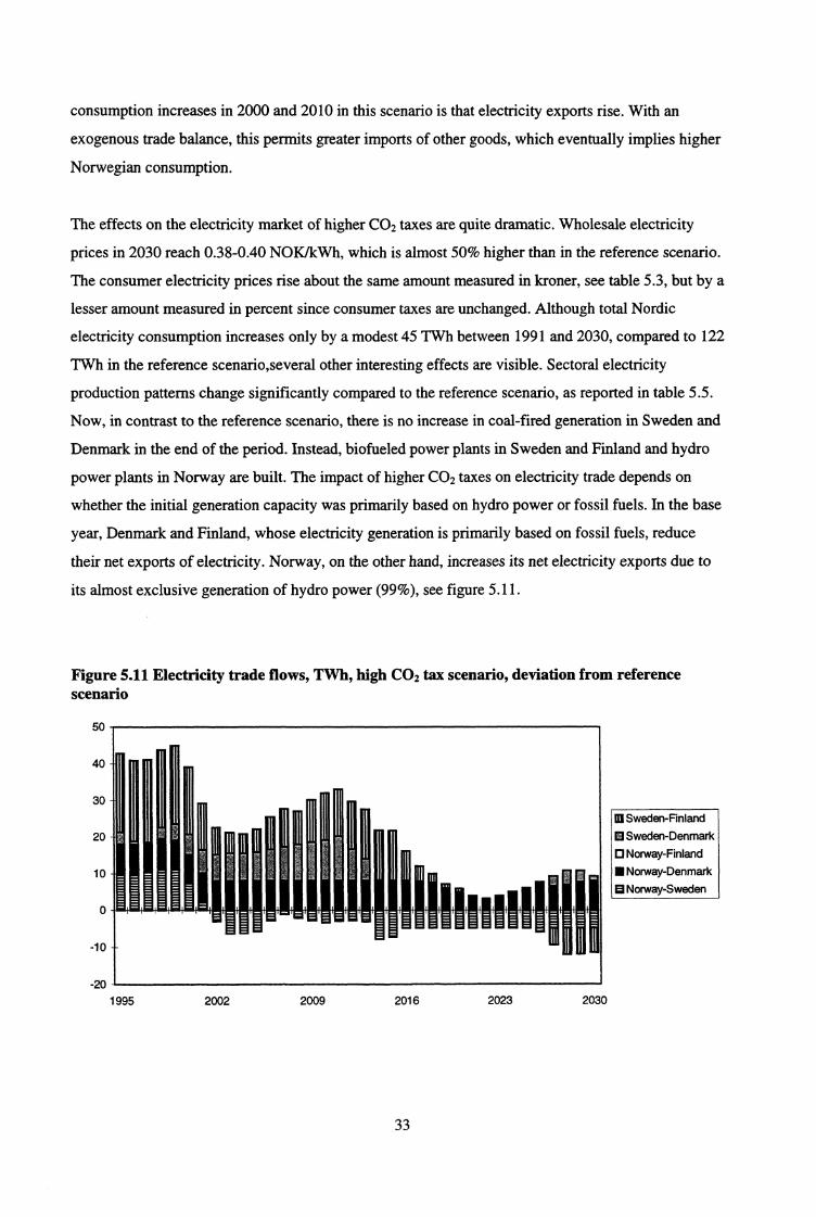
The effects on the electricity market of higher CO 2 taxes are quite dramatic. Wholesale electricity
prices in 2030 reach 0.38-0.40 NOK/kWh, which is almost 50% higher than in the reference scenario.
The consumer electricity prices rise about the same amount measured in kroner, see table 5.3, but by a
lesser amount measured in percent since consumer taxes are unchanged. Although total Nordic
electricity consumption increases only by a modest 45 TWh between 1991 and 2030, compared to 122
TWh in the reference scenario,several other interesting effects are visible. Sectoral electricity
production patterns change significantly compared to the reference scenario, as reported in table 5.5.
Now, in contrast to the reference scenario, there is no increase in coal-fired generation in Sweden and
Denmark in the end of the period. Instead, biofueled power plants in Sweden and Finland and hydro
power plants in Norway are built. The impact of higher CO 2 taxes on electricity trade depends on
whether the initial generation capacity was primarily based on hydro power or fossil fuels. In the base
year, Denmark and Finland, whose electricity generation is primarily based on fossil fuels, reduce
their net exports of electricity. Norway, on the other hand, increases its net electricity exports due to
its almost exclusive generation of hydro power (99%), see figure 5.11.
Figure 5.11 Electricity trade flows, TWh, high CO 2 tax scenario, deviation from referencescenario
50
40
30
20
10
0
WI Sweden-Finland0 Sweden-Denmarka Norway-Finland■ Norway-Denmark▪ Norway-Sweden
2002
33

In 2030, CO2 emissions under the high carbon tax scenario are 109 million tons, or a bit more than
half of their reference scenario level, as illustrated in figure 5.12. The emissions reduction here is
primarily due to the contraction of the electricity producing sector, but also, to a lesser extent, to the
reduction in (stationary) fuel oil consumption, compared with the reference scenario. (In 2030, the
reduction is 9 million tons.) The percentage reduction in CO 2 emissions in 2030 compared with the
reference scenario is greatest in Norway, with 51%. Similarly, Sweden reduces its emissions by 46%,
Denmark by 39% and Finland by 27%.
Figure 5.12 Nordic CO 2 emissions, deviation from reference scenario, million tons
3020 —
10 —0
-10 --20
-30 —-40 —-50 ---60-70 ---80 4 4 i 1 4 1 I I 1 4 f 1 I 1 I 1 i I 14 I I 14 I I I I f i 1 1 1 ill
1991 1995 1999 2003 2007 2011 2015 2019 2023 2027
Early Swedish— —nuclear phase out
CO2 tax scenario
.002 tax scenarioand early Swedishnuclear phase out
The phasing out of Swedish nuclear power
In 1980, Sweden made political decisions about the future of its nuclear power after holding a
referendum. The main point was that all Swedish nuclear power should be eliminated by the year
2010, given that a set of economic conditions were satisfied. Whether this will be carried out in
practice remains to be seen. In order to study the effects of this political decision, we re-run the
reference and CO 2 tax scenarios, this time eliminating each Swedish nuclear reactor after 25 years,
rather than 40 (as in the reference case). All other assumptions of the model remain unchanged.
In both scenarios with 25 year reactor lives (i.e. with an without higher CO2 taxes), the wholesale
electricity price are the same at the end of the period as they were for the corresponding scenarios
with 40 year nuclear plant lifetimes. This is because Swedish nuclear power is phased out by 2030
regardless. Therefore, most of the other variables are also nearly identical at the end of the period.
However, the developments over the course of the period are significant and are strongest in the
scenario without increased CO2 taxes. Thus, the results from that scenario (early Swedish nuclear
phase out without increased carbon taxes) will be focused on here. The biggest rise in wholesale
34

electricity prices per kWh with Swedish reactor phase out after 25 years' use is 0.04 NOK compared
to the reference scenario and 0.03 NOK compared with the higher CO2 tax scenario.
As table 5.4 reveals, total Nordic electricity consumption patterns remain basically unchanged
compared to the reference scenario, winding up about 1% lower by the end of the period. Production
patterns, however, show more noticeable changes. In Sweden, gas power, CHP, and gas turbine
generation methods pick up the slack which results from the earlier nuclear plant shutdowns. The
upward trend for these methods starts in about 2010, as opposed to in 2020 for the reference scenario.
Denmark also demonstrates a new production pattern, using substantially more gas power beginning
in about 2002, rather than stepping up gas power production in 2020, as in the reference scenario.
Trade patterns under early Swedish nuclear plant shut down (with base year carbon taxes) are
significantly changed, see figure 5.13. Sweden exports considerably less electricity to Finland in the
beginning of the period than in the reference scenario, and imports from Finland between 2006-2016,
something which does not occur at all in the reference scenario. In addition, as would be expected,
Sweden also starts importing electricity from Denmark earlier than in the reference scenario, now
starting in 2001 and remaining fairly stable at about 16 Twh for the rest of the period.
Figure 5.13 Electricity trade flows, TWh, early Swedish nuclear phase-out scenario, deviationfrom reference scenario
1E1 Sweden-Finland
▪ Sweden-Denmark
0 Norway-Finland
■ Norway-Denmark
B Norway-Sweden
CO2 emissions are affected in two ways by Swedish reactor phase outs: first, power generation based
on fossil fuels rises which increases CO 2 emissions. Second, because electricity prices increase,
consumers substitute somewhat away from electricity and towards the (stationary) use of fuel oils,
which also leads to higher CO 2 emissions, see figure 5.12. The largest reduction in Nordic GDP
35

resulting from the phasing out of Swedish nuclear reactors is around 0.37% compared to the
reference scenario and around 0.21% compared to the higher CO 2 tax scenario. In Norway and
Sweden, the reduction in GDP is greatest around 2010, when all Swedish nuclear power generation is
eliminated. With increased carbon taxes and earlier nuclear plant closures, the largest GDP reduction
occurs a few years earlier in Denmark and Finland than in Norway and Sweden.
6. ConclusionsIn an earlier partial Nordic energy market model, the interaction between the Nordic electricity market
and the rest of the economy was not integrated. NORMEN was designed to take these interaction
aspects into account. The energy markets are modeled in the same way as the earlier partial model,
while the main elements of the macro module are as in traditional CGE models. To keep the model
structure simple, we use elementary functional forms for important macro variables. Most sectors
have a Cobb-Douglas production structure with constant returns to scale and no excess profits. Trade
(except of electricity) is modeled according to the Armington hypothesis, i.e. domestic and foreign
goods are imperfect substitutes. The trade balance and government consumption are treated
exogenously. The level of total consumption is determined such that there is equilibrium in the goods
markets. NORMEN's model structure, databases and calibration methods are documented in this
report.
Using NORMEN, we analyze the effects on the Nordic electricity market and on the Nordic
economies of increased CO 2 taxes and/or early Swedish nuclear reactor shut downs. Compared with
the earlier partial Nordic energy market model, in NORMEN electricity consumption is more
sensitive to electricity price changes because the substitution between energy and other production
factors such as labor, capital and intermediates is an integrated part of the model. An increase in the
electricity price resulting from higher CO 2 taxes and/or early Swedish nuclear reactor phase out has
only modest effects on important macro variables such as GDP and consumption. In the long run, the
reduction in GDP is around 1% when the electricity price rises by 50%. This is because the cost of
electricity for most sectors is only a small fraction of total factor outlays. Even for the most
electricity-intensive sectors in NORMEN, the electricity cost share is not greater than 10%. This
means that the price of produced inputs, such as capital and intermediates, changes very little with
large electricity price increases. Thus, the amount of capital and intermediates demanded by
producers also scarcely changes. By introducing a common Nordic CO 2 tax of 350 NOK (around 55
USD) per ton CO2, total Nordic stationary CO 2 emissions fall by about 40%. Most of this reduction
occurs in the power generation sector (coal, oil, and gas fired). But the use of oil for stationary
purposes falls, which also reduces CO 2 emissions.
36

In future model versions, it is very important to improve the description of the connection between
electricity prices and electricity consumption in the production sectors. This version of the model
probably exaggerates how strongly electricity consumption reacts to electricity price changes, while
the production scale effects may be underestimated. The closure mechanism in this version of the
model implies that key variables, such as consumption and investment, vary cyclically around the
trend in the short run. In the long run, however, the model is reasonably robust. In any case, the
closure mechanism still ought to be improved. One possible way to do this might be to maximize total
discounted Nordic consumption over the entire scenario period, rather than maximizing the sum of
consumer and producer surplus in the electricity market, as in done in this version of NORMEN.
Another possible improvement to the model would be to integrate the variations in electricity demand
and production over the day/week/season, something which is an important feature of 'real' electricity
markets. Such an improvement is very important in order to describe electricity trade patterns and
would better reflect the variation in the short term marginal costs in the interplay especially between
hydro power and thermal power.
ReferencesAune, F.R., T. Bye and T.A. Johnsen (1995): Kostnader ved negleggelse av svenske atomkraftverk,Økonomiske analyser 7/95, Statistics Norway, 3-10.
Aasness, J. and B. Holtsmark (1993): Consumer Demand in MSG-5, Notater 93/46, Statistics Norway.
Bank of Finland (1990): The BOF4 Quarterly Model of the Finnish Economy, D:73.
Board of Customs (1992): Foreign Trade 1991, Vol. 2, Finland.
Brooke, A., D. Kendrick and A. Meeraus (1992): GAMS: A User's guide - Release 2.25, SanFrancisco: The Scientific Press.
Bye, T., E. Gjelsvik, T.A. Johnsen, S. Kverndokk and H.T. Mysen (1995): CO2 utslipp og detnordiske elektrisitetsmarkedet. En modellanalyse, Temallord rapport 1995:539, Nordic Council ofMinisters.
Bye, T. and T.A. Johnsen (1995): Prospects for a Common, Deregulated Nordic Electricity Market,Discussion Papers 144, Statistics Norway.
Danish Economic Council (1994): SMEC-Modeldokumentation og beregnede virkninger ofØkonomisk politik.
Danish Economic Council (1995a): GESMEC-En Generel Ligevcegtsmodel for Danmark,Dokumentation og anvendelser.
Danish Economic Council (1995b): created a database for us, Norge-06117 on 13-03-95.
Danmarks Statistik (1994): Input-output labeller og analyser 1990.
37
Danmarks Statistik (1995): Nationalregnskabsstatistik 1993.
Gjelsvik, E. (1993): Kraftmarkedene i Norden, Dokumentajonsnotat for Nordiskenergimarkedsmodell, Statistics Norway.
Holmoy, E., G. Norden and B. Strom (1994): MSG-5; A Complete Description of the System ofEquations, Reports 94/19, Statistics Norway.
Lindquist, K.G. (1993): Empirical Modelling of Exports of Manufactures: Norway 1962-1987,Reports 93/18, Statistics Norway.
Mysen, H.T. (1994): Brukerveiledning for Nordisk energimarkedsmodell med modellfil, datafil ogutskriftsfil, Statistics Norway.
Mysen, H.T. (1995): Nordisk energimarkedsmodell, Dokumentasjon av delmodell forenergietterspOrsel i industrien, Notater 95/24, Statistics Norway.
Mwhle, N.Ø. (1992): KrysslOpsdata og krysslopsanalyse 1970-1990, Reports 92/26, StatisticsNorway.
Naug, B.E. (1994): An Econometric Analysis of the Development of Manufacturing Import Shares1968-1990, Social and Economic Studies 84, Statistics Norway.
National Institute of Economic Research (1996): sent us data for Sweden.
Nordel (1986-1993): Arsberetninger 1986-1993, Nordel.
Nordic Statistical Secretariat (1993): Yearbook of Nordic Statistics, Vol.31.
Nordic Statistics (1995): Statistics on CD-ROM.
Norwegian Water and Energy Board (1994): Statistikk over overforingstariffer i regional- ogdistribusjonsnett.
OECD (1994): Flows and Stocks of Fixed Capital 1967-1992, Statistics Directorate.
Statistics Finland (1994a): Energy Statistics 1993, Energy 1994:1.
Statistics Finland (1994b): Financial Statements Statistics 1992, Enterprises 1994:2.
Statistics Finland (1995a): Input-output 1992, National Accounts 1995:9.
Statistics Finland (1995b): National Accounts 1989-1994, Tables 1995:14.
Statistics Finland (1995c): Population projection by municipalities 1995-2030.
Statistics Finland (1992-3d): Statistical Yearbook 1992 & 1993.
Statistics Norway (1993): Nasjonalregnskapsstatistikk 1991, Official Statistics of Norway NOS C83.
Statistics Sweden (1995): BNPs anvanding 1980-1993, Appendix 1 til Nationalrakenskaper 1980-1993 N10 SM 9401.
38
Statistics Sweden (1993a): El-, gas- ockfitirrviirmefOrsOrjningen 1991, Statistiska meddelanden E 11SM 9301.
Statistics Sweden (1993b): Industri 1991, Del 1.
Statistics Sweden (1995): Nationalriikenskaper 1980-1993, N10 SM 9401.
Statistics Sweden (1994a): Produktion och sysselsiittning, detaljerade labeller 1980-1992, Appendix2 til Nationalrakenskaper 1980-1992 N10 SM 9301.
Statistics Sweden (1994b): Realkapitalstock 1980-1994, Appendix 3 til Nationalrakenskaper 1980-1993 N 10 SM 9401.
Statistics Sweden (1993a): Statistisk drsbok '94.
Statistics Sweden (1993b): Arliga energibalanser 1990-1991, Statistiska meddelanden E 20 SM 9302.
Varian H. R. (1984): Microeconomic Analysis, New York: Norton.
39

Issued in the series Documents
95/2 E. Gjelsvik, T. Johnsen, H.T. Mysen andA. Valdimarsson (1995): Energy Demand inIceland
95/3 C. Zhao, 0. Bjerkholt, T. Halvorsen andY. Zhu (1995): The Flow of Funds Accounts inChina
95/4 Nordic Indicator Group (1995): NordicEnvironmental Indicators. Draft document.English version with main points from commentsreceived
95/5 H.A. Gravningsmyhr (1995): Analysing Effects ofRemoving Survivors' Pensions, Using theMicrosimulation Model LOTTE
95/6 P. Boug (1995): User's Guide. The SEEM-modelVersion 2.0
95/7 E. Bowitz, N.O. Maehle, V.S. Sasmitawidjaja andS.B. Widoyono (1995): MEMLI — AnEnvironmental model for Indonesia. TechnicalDocumentation of data programs and procedures
95/8 K. H. Alfsen, T. Bye, S. GlomsrOd and H. Wiig(1995): Integrated Assessment of Soil Degradationand Economic Growth in Ghana
95/9 0. Bjerkholt (1995): Ragnar Frisch and theFoundation of the Econometric Society andEconometrica
95/10 P.J. Bjerve (1995): The Influence of RagnarFrisch on Macroeconomic Planning and Policy inNorway
96/1 D. Kolsrud (1996): Documentation of ComputerPrograms that Extend the SEEM Model andProvide a Link to the RAINS Model
96/2 E. Bowitz, V.S. Sasmitawidjaja and G. Sugiarto(1996): The Indonesian Economy and Emission ofCO2: An Analysis Based on the Environmental-Macroeconomic-Model MEMLI, 1990-2020
96/3 H.V. Swbo (1996): Use of GeographicalInformation Systems (GIS) in Statistics Norway
96/4 E. Berg (1996): Some Results from the Literatureon the Impact of Carbon Taxes on the PetroleumWealth
96/5 E.J. FlOttum (1996): Norwegian NationalAccounts — Documentation of the Compilationand Methods Applied. I General Description. IIGDP From the Output Approach
96/6 E.J. FlOttum (1996): Norwegian NationalAccounts — Documentation of the Compilation
and Methods Applied. III GDP by ExpenditureApproach. IV GDP by Income Approach
96/7 0. Bjerkholt, K.A. Brekke and R. Choudhury(1996): The Century Model - on the Long TermSustainability of the Saudi Arabian Economy
96/8 R. Choudhury (1996): The Century Model.Technical Documentation of Computer Programsand Procedures
96/9 R. Choudhury and K.A. Magnussen (1996): TheImplementation Model. Technical Documentationof Computer Programs and Procedures
96/10 R. Choudhury (1996): The Selection Model.Technical Documentation of Computer Programsand Procedures
96/11 R. Choudhury (1996): The 0M95 — An Oil Modelfor the Kingdom of Saudi Arabia. TechnicalDocumentation of Computer Programs andProcedures
96/12 K. Nyborg (1996): Environmental Valuation,Cost-Benefit Analysis and Policy Making: ASurvey
96/13 P.R. Johansen and K.A. Magnussen (1996): TheImplementation Model. A Macroeconomic Modelfor Saudi Arabia
96/14 A. Capplen and K. A. Magnussen (1996): TheSelection Model. A General Equilibrium Modelfor Saudi Arabia
96/15 P. Boug and L. Brubakk (1996): Impacts ofEconomic Integration on Energy Demand andCO2 emissions in Western Europe
96/16 J.K. Dagsvik (1996): Probabilistic Models forQualitative Choice Behavior: An Introduction
96/17 K.H. Alfsen and K.E. Rosendahl (1996):Economic Damage of Air Pollution
96/18 K.H. Alfsen (1996): Why Natural ResourceAccounting?
96/19 F. R. Aune, T. Bye, T.A. Johnsen and A. Katz(1996): NORMEN: A General Equilibrium Modelof the Nordic Countries Featuring a DetailedElectricity Block
40

Documents
Statistics NorwayResearch DepartmentP.O.B. 8131 Dep.N-0033 Oslo
Tel.: + 47-22 86 45 00Fax: + 47-22 11 12 38
ISSN 0805-9411
Statistics Norway