Omni-Wrist III – A New Generation of Gimbals Systems: Control

J. Sofka+, V. Skormin+, V. Nikulin+, D. Nicholson†

+Dept. of Electrical and Computer Engineering, SUNY Binghamton, Vestal Parkway E, Binghamton, NY 13902-6000

†AFRL, 525 Brooks Rd., Rome, NY 13441-4505

ABSTRACT The Omni-Wrist III robotic manipulator, inspired in design by the kinematics of the human wrist, represents with the full 180º hemisphere of singularity free range a very capable alternative to traditional gimbals systems. Research efforts at the Laser Communications Research Laboratory at Binghamton University have resulted in the establishment of an accurate mathematical model, which was utilized in the development of control systems presented in this paper. A state variable controller and two linear model following controllers are developed and evaluated. The third controller is designed to achieve full decoupling of the highly coupled system. The adaptation and disturbance rejection capabilities of the controllers are demonstrated through friction compensation. Keywords: Omni-Wrist III, gimbals, control, reference model, full decoupling

1 INTRODUCTION

Rising demand for communication bandwidth, together with the need for covert data links belong to the main driving forces for the research in the area of free space laser communications [1][2][3]. Along with the benefits inherent from the laser beam being used as a communications medium comes the challenge of pointing the laser beam accurately and with a high degree of agility in order to maintain the laser link, and over a wide range to be able to acquire links in various relative positions. While the requirement for high steering bandwidth can be addressed by utilizing piezo-electric fast steering mirrors or non-mechanical beam steering devices such as Bragg cells and solutions based on liquid crystal arrays, the wide steering range requirement can not be met by the limited range of these devices. Gimbals were proposed to be used in combination with fast steering devices to satisfy both the frequency and range requirements [4]. Traditional gimbal systems benefit from the design intention of decoupled operation but suffer from singularity, relatively high inertia, cable routing difficulties, and limited range and accuracy. A novel gimbal-like design entitled Omni-Wrist III (Figure 1), developed by Ross-Hime Designs [5], attempts to address the disadvantages of traditional gimbals with a device capable of operating over a full 180º hemisphere of yaw/pitch motion. The evolution-inspired mechanical design of the singularity-free, two-degrees-of- freedom manipulator features two linear actuators attached to the links of the structure similar to the attachment of muscles to bones in biological structures. The absence of gears frees the device from backlash. Exhibiting reduced response time in comparison with traditional gimbals systems and featuring convenient through-the-center-hole wiring, the Omni-Wrist III has the potential of revolutionizing gimbal positioning. The benefits outweigh the single drawback of the increased complexity of the structure. Advanced control concepts need to be employed in order to fully exploit the potential of the manipulator. Building on the mathematical model developed in [6], this paper focuses on the design and evaluation of three controllers with increasing levels of complexity and improving performance. First, a state variable controller was implemented, followed by two linear model following controllers. The first two controllers are designed to perform steady state decoupling; the third controller handles full decoupling of the highly coupled two-input-two-output system.

Figure 1 Omni-Wrist III Robotic Manipulator

2 STATE VARIABLE CONTROLLER

It was established in [6] that the Omni-Wrist III can be accurately modeled as two actuators coupled with the kinematic relationship given by the structure of the device as shown in Figure 2, where u1 and u2 represent the input voltages driving the servo amplifiers, Ax1 and Ax2 the linear displacement of the actuators, and Az and Dec represent the azimuth and declination of the sensor mount. The servo amplifiers power the actuators so that the actuator brushless linear motors deliver force proportional to the input voltage. The actuator dynamics can be modeled by second order systems with Coulomb friction as shown in Figure 3, where a = 3.9⋅106, b = 35, and f = 0.76 for Actuator 1 and a = 3.2⋅106, b = 22, and f = 0.49 for Actuator 2 [6].

Actuator 1Dynamics

Actuator 2Dynamics

Omni-Wrist IIIKinematics

Ax1

Ax2

u1

u2

Az

Dec

Figure 2 Omni-Wrist III System Diagram

Figure 3 Model of the Dynamics of the Actuators [6]

A linearized state variable description was used for the development of the controllers in the form

ainput voltage

output position

1ss + b

f

sign

2

FxWruCxy

BuAxx

−==

+=&

(1)

where u is the input voltage, the state vector x is comprised of the velocity and the position of the linear actuator, and the output y is the position of the actuator. A controller matrix F was introduced, placing the dominant eignevalues of the closed loop fundamental matrix (A – BF) to –20 ± 12j. A matrix W was chosen to eliminate the steady state tracking error for a step reference. Figure 4 captures the configuration of the closed loop system with the state variable controller. Notice that there are two independent control channels, one for each actuator. The cross coupling is caused by the kinematic structure of the manipulator and doesn’t penetrate through the actuators. Steady state decoupling is achieved by the transformation of the azimuth/declination coordinates into the coordinates of the displacement of the linear actuators by the means of the Inverse Kinematics block. The blocks between the Axis Reference and Axis Position points represent the closed loop system comprised of the actuators and their respective controllers. The Axis Position is the actual value read from the quadrature encoder feedback sensor, while the second state, the velocity, is calculated numerically as

[ ] [ ]T

nxnxnv 1][ −−= , (2)

where T is the sampling time, x the position, and n the time index.

AzimuthInverse

KinematicsDeclination

Axis 1Reference

Axis 2Reference

Axis 1Position

ForwardKinematics

Axis 2Position

Azimuth

Declination

F

B C

A

-

F

B C

A-

W

W

Motor 2

Motor 1

Figure 4 State Variable Controller

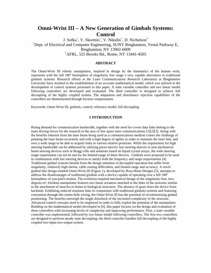
The Forward Kinematics block represents the kinematics of the device and in simulation allows for the evaluation of the pointing angle in the azimuth/declination coordinates (there are no feedback sensors measuring these values directly). While the design of the state variable controller is simple, its performance leaves hope of its successful application unfulfilled, mainly due to the inability to compensate for the effects of friction. The controller was designed to ensure operation in the non-saturated range of control signals for a step reference of about 50 degrees, providing a controller gain not sufficiently large to compensate for the friction forces, and resulting in the failure to meet the design requirements. The ability to improve the disturbance rejection capabilities by increasing the controller gain is reduced by the physical limits of the actuators. The response of the system captured in Figure 5 was obtained as follows: First the system was driven by a step reference in the declination channel from 20 degrees to 60 degrees (Figure 5 (b)) followed by a step reference in the azimuth channel from 60 degrees to 100 degrees (Figure 5 (a)). A sufficient time was set between the two steps to allow the transient process of the declination channel to settle before the excitation in the azimuth channel. An inspection of the response of the closed loop system in the linear motor displacement coordinates (Figure 5 (e), (f)) reveals the shortcomings of the state variable controller. The

3

expected behavior of the closed loop system, represented by the dashed line, is far from being achieved by the state variable controller. This is caused by the friction forces, which represent a phenomenon not taken into account in the controller design process. The controller generates a small control effort for a small variation in the reference signal, which may not suffice to overcome the friction force and cause movement of the actuator. This can be observed in the second half of the response of the second axis in Figure 5 (f).

0 100 200 300 400 500 600 700 800 900 1000 110050

60

70

80

90

100

110Azimuth reference

Time [x.5 ms]

Azimuth [deg]

0 100 200 300 400 500 600 700 800 900 1000 110010

20

30

40

50

60

70Declination reference

Time [x.5 ms]

Declination [deg]

0 100 200 300 400 500 600 700 800 900 1000 1100-1

-0.5

0

0.5

1

1.5

2

2.5

3x 104 Axis 1 response

Time [x.5 ms]

Encoder position

modelplant

0 100 200 300 400 500 600 700 800 900 1000 1100-5

-4.5

-4

-3.5

-3

-2.5

-2

-1.5

-1x 104 Axis 2 response

Time [x.5 ms]

Encoder position

modelplant

(a) (b)

0 100 200 300 400 500 600 700 800 900 1000 110050

60

70

80

90

100

110Azimuth response

Time [x.5 ms]

Azimuth [deg]

0 100 200 300 400 500 600 700 800 900 1000 110010

20

30

40

50

60

70Declination response

Time [x.5 ms]

Declination [deg]

(c) (d)

(e) (f)

Figure 5 Response of the Closed Loop System with a State Variable Controller

4

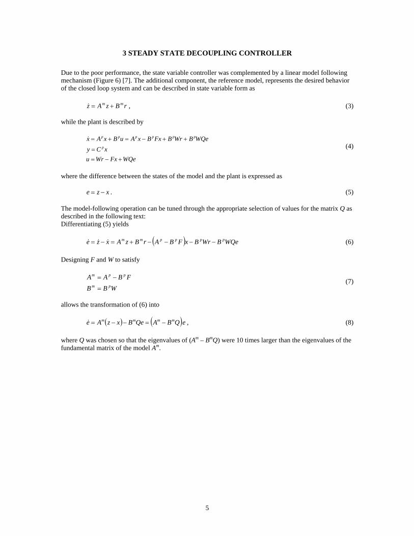
3 STEADY STATE DECOUPLING CONTROLLER

Due to the poor performance, the state variable controller was complemented by a linear model following mechanism (Figure 6) [7]. The additional component, the reference model, represents the desired behavior of the closed loop system and can be described in state variable form as

rBzAz mm +=& , (3)

while the plant is described by

WQeFxWruxCy

WQeBWrBFxBxAuBxAxp

pppppp

+−==

++−=+=& (4)

where the difference between the states of the model and the plant is expressed as

xze −= . (5)

The model-following operation can be tuned through the appropriate selection of values for the matrix Q as described in the following text: Differentiating (5) yields

( ) WQeBWrBxFBArBzAxze ppppmm −−−−+=−= &&& (6)

Designing F and W to satisfy

WBB

FBAApm

ppm

=

−= (7)

allows the transformation of (6) into

( ) ( eQBAQeBxzAe mmmm −=−−=& ) , (8)

where Q was chosen so that the eigenvalues of (Am – BmQ) were 10 times larger than the eigenvalues of the fundamental matrix of the model Am.

5

InverseKinematics

Axis 1Reference

Axis 2Reference

Axis 1Position

ForwardKinematics

Axis 2Position

Azimuth

Declination

F

-

F

-

Q

Bm

Am

-

Cp

Ap

Bp

ReferenceModel

Bp

Ap

Cp

Bm

AmReferenceModel

Q-

Azimuth

Declination

W

W

Motor 1

Motor 2

Figure 6 Steady State Decoupling Controller

The performance of the linear model following controller can be evaluated by inspecting the responses in Figure 7. The reference signals for azimuth and declination were identical to the reference signals utilized to obtain the response of the state variable controller in the previous section, to allow for the possibility of side-by-side comparison. Notice that due to the decoupling functionality, both motors are energized in each of the steps (Figure 7 (e) and (f)), and the system is decoupled in steady state. In the transient process, however, there is noticeable cross coupling in the azimuth channel when the system was driven by declination reference (Figure 7 (c)) and in the declination channel when the system was driven by azimuth reference (Figure 7 (d)). The effect of the unmodeled friction forces is compensated for by the linear model following controller through the elimination of the error between the state of the model and the state of the plant by the means of the matrix Q. Section 5 of this paper focuses on friction compensation in more detail. The performance of the closed loop system, limited by the power of the linear actuators, can be adjusted by modifying the reference model to achieve different combinations of range and bandwidth. For a 10 degree range, a bandwidth of about 9 Hz can be achieved, 5 degree range allows for a bandwidth of about 14 Hz, and for a 1 degree sinusoid reference the maximum bandwidth is about 27 Hz.

6

0 100 200 300 400 500 600 700 800 900 1000 110050

60

70

80

90

100

110Azimuth reference

Time [x.5 ms]

Azimuth [deg]

0 100 200 300 400 500 600 700 800 900 1000 110010

20

30

40

50

60

70Declination reference

Time [x.5 ms]

Declination [deg]

0 100 200 300 400 500 600 700 800 900 1000 110010

20

30

40

50

60

70Declination response

Time [x.5 ms]

Declination [deg]

0 100 200 300 400 500 600 700 800 900 1000 110050

60

70

80

90

100

110Azimuth response

Time [x.5 ms]

Azimuth [deg]

0 100 200 300 400 500 600 700 800 900 1000 1100-1

-0.5

0

0.5

1

1.5

2

2.5

3x 104 Axis 1 response

Time [x.5 ms]

Encoder position

modelplant

(a) (b)

(c) (d)

0 100 200 300 400 500 600 700 800 900 1000 1100-5

-4.5

-4

-3.5

-3

-2.5

-2

-1.5

-1x 104 Axis 2 response

Time [x.5 ms]

Encoder position

modelplant

(e) (f)

Figure 7 Response of the Steady State Decoupled System

4 FULL DECOUPLING CONTROLLER

A full decoupling controller derived from the steady state decoupling controller was developed and is also based on the linear model following control principle. The design of the full decoupling controller (Figure 8) differs from the design of the steady state decoupling controller (Figure 6) in the placement of the reference model. In the steady state decoupling controller, the reference in azimuth/declination coordinates

7

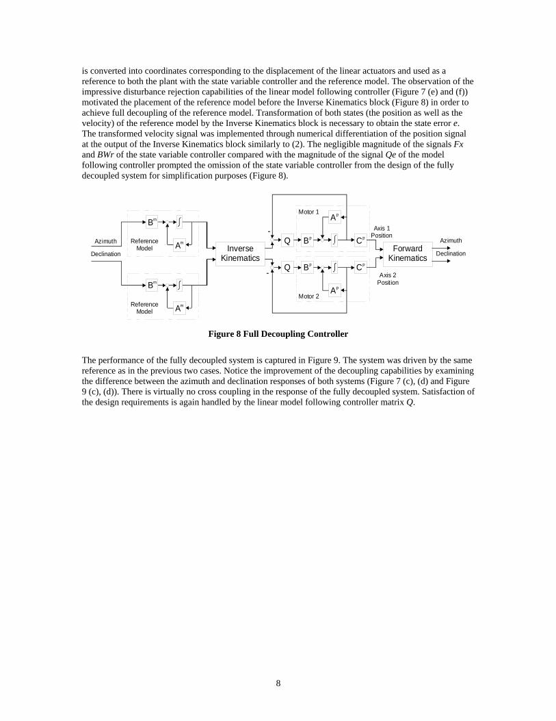
is converted into coordinates corresponding to the displacement of the linear actuators and used as a reference to both the plant with the state variable controller and the reference model. The observation of the impressive disturbance rejection capabilities of the linear model following controller (Figure 7 (e) and (f)) motivated the placement of the reference model before the Inverse Kinematics block (Figure 8) in order to achieve full decoupling of the reference model. Transformation of both states (the position as well as the velocity) of the reference model by the Inverse Kinematics block is necessary to obtain the state error e. The transformed velocity signal was implemented through numerical differentiation of the position signal at the output of the Inverse Kinematics block similarly to (2). The negligible magnitude of the signals Fx and BWr of the state variable controller compared with the magnitude of the signal Qe of the model following controller prompted the omission of the state variable controller from the design of the fully decoupled system for simplification purposes (Figure 8).

Azimuth

Declination

Bm

AmReferenceModel

Bm

AmReferenceModel Inverse

Kinematics

- Bp

Ap

Cp

Q-

Cp

Ap

Bp

Q

Axis 1Position

ForwardKinematics

Axis 2Position

Azimuth

Declination

Motor 1

Motor 2

Figure 8 Full Decoupling Controller

The performance of the fully decoupled system is captured in Figure 9. The system was driven by the same reference as in the previous two cases. Notice the improvement of the decoupling capabilities by examining the difference between the azimuth and declination responses of both systems (Figure 7 (c), (d) and Figure 9 (c), (d)). There is virtually no cross coupling in the response of the fully decoupled system. Satisfaction of the design requirements is again handled by the linear model following controller matrix Q.

8

0 100 200 300 400 500 600 700 800 900 1000 1100-5

-4.5

-4

-3.5

-3

-2.5

-2

-1.5

-1x 104 Axis 2 response

Time [x.5 ms]

Encoder position

modelplant

0 100 200 300 400 500 600 700 800 900 1000 1100-1

-0.5

0

0.5

1

1.5

2

2.5

3x 104 Axis 1 response

Time [x.5 ms]

Encoder position

modelplant

0 100 200 300 400 500 600 700 800 900 1000 110010

20

30

40

50

60

70Declination response

Time [x.5 ms]

Declination [deg]

modelplant

0 100 200 300 400 500 600 700 800 900 1000 110050

60

70

80

90

100

110Azimuth response

Time [x.5 ms]

Azimuth [deg]

modelplant

0 100 200 300 400 500 600 700 800 900 1000 110010

20

30

40

50

60

70Declination reference

Time [x.5 ms]

Declination [deg]

0 100 200 300 400 500 600 700 800 900 1000 110050

60

70

80

90

100

110Azimuth reference

Time [x.5 ms]

Azimuth [deg]

(a) (b)

(c) (d)

(e) (f)

Figure 9 Response of the Full Decoupling Controller

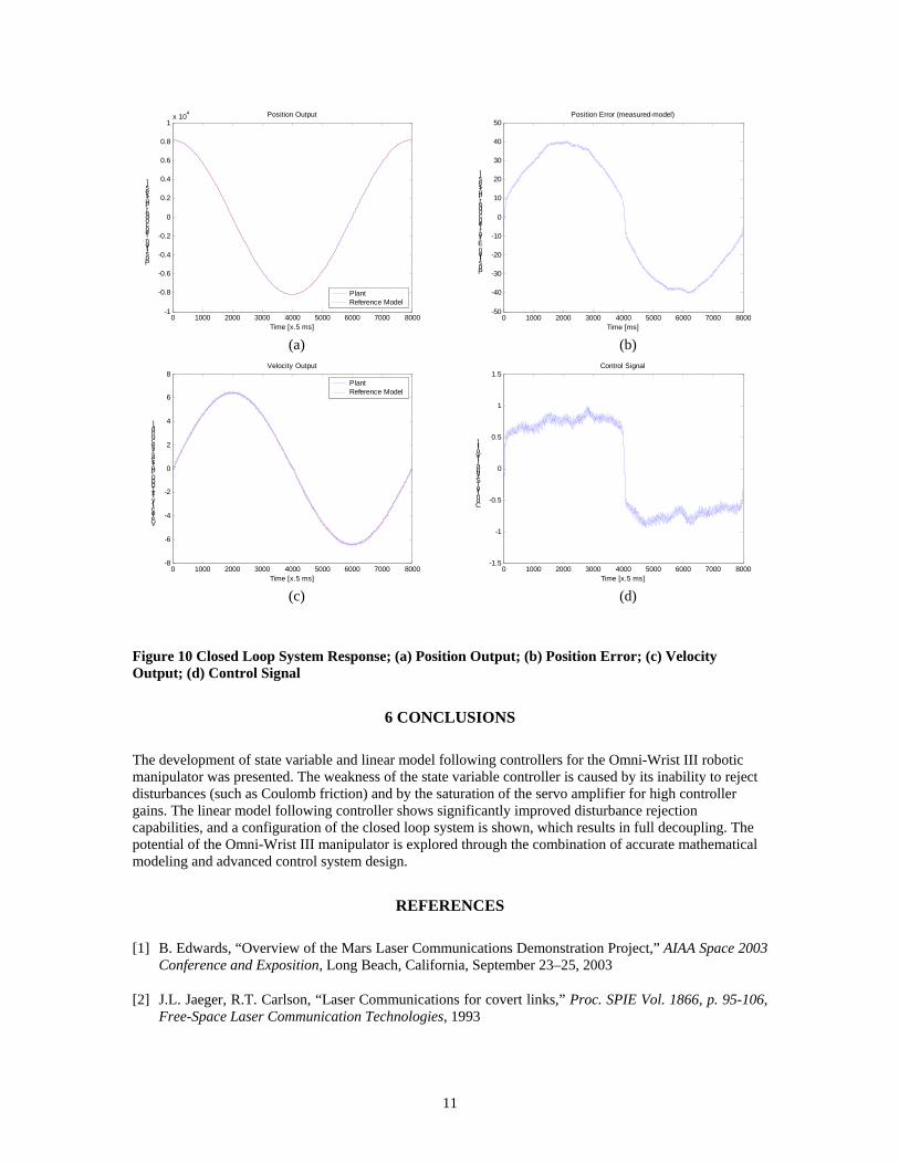
5 DISTURBANCE REJECTION

In order to evaluate the disturbance rejection (and friction compensation) capabilities, the closed loop system was driven by a low frequency sinusoidal signal in the actuator linear displacement coordinates. The slow variation of the reference signal results in a slow motion of the actuators, magnifying the effect of the compensation of the friction forces in the control signal.

9

A period of 4 seconds and an amplitude of 8192 pulses (which corresponds to a declination of about 10 degrees of the Omni-Wrist III sensor mount) were chosen for the reference signal in this experiment. Figure 10 captures the performance of the control system. While the effects of noise on the performance of the control system are mitigated by the inertia of the actuators, the disturbance rejection capability of the control system becomes more apparent when the noise in the collected signals is reduced. Therefore, off-line averaging was applied to the periodic position, velocity, and control signals in order to reduce noise and clarify the plots. The response amounting to one million samples each of the position, velocity, and control signals with a period of 8000 samples was averaged over 125 realizations as

[ ] [ ] [ ]( ) ,7999,,1,0,80008000125

1 124

0∑=

=+++=k

nnkwnkuns K (9)

where u[8000k + n] represents the true position, velocity, or control signal, s[n] represents the averaged signal, and w[8000k + n] represents the noise in the position, velocity, and control signals. The variance of the noise present in the averaged signals was reduced as

,125

1 22ws σσ =

where σw2 represents the variance of the noise present in the position, velocity and control signals and σs

2 represents the variance of the noise present in the averaged signal. The position output of the closed loop system, as well as the reference model, is shown in Figure 10 (a), and the position error signal is shown in Figure 10 (b). The amplitude of the error translates to about 1 mrad pointing angle lag. The velocity response of the closed loop system, as well as that of the reference model, are shown in Figure 10 (c), where the effect of the change in polarity of the Coulomb friction is slightly noticeable at the time of 2 seconds. The disturbance rejection capability of the control system is represented in the control signal (Figure 10 (d)). The polarity change of the Coulomb friction signal is clearly visible in Figure 10 (d). The disturbance rejection capability is limited by the magnitude of the high frequency noise in the feedback signals. The noise magnitude can be significantly reduced through the application of an appropriate filtering scheme, such as one employing a Kalman filter. The denoising performance of the filter is bounded by the sampling frequency, which for the hardware utilized in this project is 2 kHz. Implementation of the control schemes described in this paper on faster hardware would allow for even better adaptation and disturbance rejection performance.

10

0 1000 2000 3000 4000 5000 6000 7000 8000-1

-0.8

-0.6

-0.4

-0.2

0

0.2

0.4

0.6

0.8

1x 104 Position Output

Time [x.5 ms]

Position [encoder pulses]

PlantReference Model

0 1000 2000 3000 4000 5000 6000 7000 8000-8

-6

-4

-2

0

2

4

6

8Velocity Output

Time [x.5 ms]

Velocity [x1000 pulses/second]

PlantReference Model

0 1000 2000 3000 4000 5000 6000 7000 8000-50

-40

-30

-20

-10

0

10

20

30

40

50Position Error (measured-model)

Time [ms]

Position Error [encoder pulses]

0 1000 2000 3000 4000 5000 6000 7000 8000-1.5

-1

-0.5

0

0.5

1

1.5Control Signal

Time [x.5 ms]

Control Signal [Volt

(a) (b)

]

(c) (d)

Figure 10 Closed Loop System Response; (a) Position Output; (b) Position Error; (c) Velocity Output; (d) Control Signal

6 CONCLUSIONS

The development of state variable and linear model following controllers for the Omni-Wrist III robotic manipulator was presented. The weakness of the state variable controller is caused by its inability to reject disturbances (such as Coulomb friction) and by the saturation of the servo amplifier for high controller gains. The linear model following controller shows significantly improved disturbance rejection capabilities, and a configuration of the closed loop system is shown, which results in full decoupling. The potential of the Omni-Wrist III manipulator is explored through the combination of accurate mathematical modeling and advanced control system design.

REFERENCES

[1] B. Edwards, “Overview of the Mars Laser Communications Demonstration Project,” AIAA Space 2003 Conference and Exposition, Long Beach, California, September 23–25, 2003

[2] J.L. Jaeger, R.T. Carlson, “Laser Communications for covert links,” Proc. SPIE Vol. 1866, p. 95-106, Free-Space Laser Communication Technologies, 1993

11

[3] H. Hemmati, K. Wilson, M. Sue, L. Harcke, M. Wilhelm, C.-C. Chen, J. R. Lesh, Y. Feria, D. Rascoe, F. Lansing, J. Layland, “Comparative Study of Optical and Radio-Frequency Communication Systems for a Deep-Space Mission,” TDA Progress Report, February, 1997

[4] J. Sofka, V. Nikulin, V. Skormin, D. Nicholson, “Hybrid Laser-Beam Steerer for Laser Communications Applications,” The International Symposium on Optical Science and Technology, SPIE’s 48th Annual Meeting, San Diego, California, August 3–8, 2003

[5] M.E. Rosheim, G.F. Sauter, “New High-Angulation Omni-Directional Sensor Mount,” SPIE Conference Proceedings. Seattle, 2002.

[6] J. Sofka, V. Skormin, V. Nikulin, D. Nicholson, “Omni-Wrist III – A New Generation of Gimbals Systems: Mathematical Modeling,” publication pending

[7] Y. D. Landau, Adaptive Control. The Model Reference Approach, Marcel Dekker, 1979

12