Embed Size (px)
Citation preview
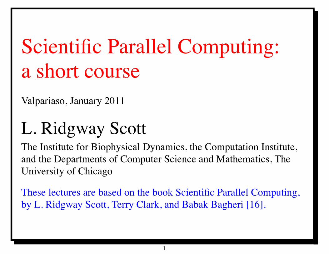
Scientific Parallel Computing:a short courseValpariaso, January 2011
L. Ridgway ScottThe Institute for Biophysical Dynamics, the Computation Institute,and the Departments of Computer Science and Mathematics, TheUniversity of Chicago
These lectures are based on the book Scientific Parallel Computing,by L. Ridgway Scott, Terry Clark, and Babak Bagheri [16].
1
1 Top 500 supercomputers
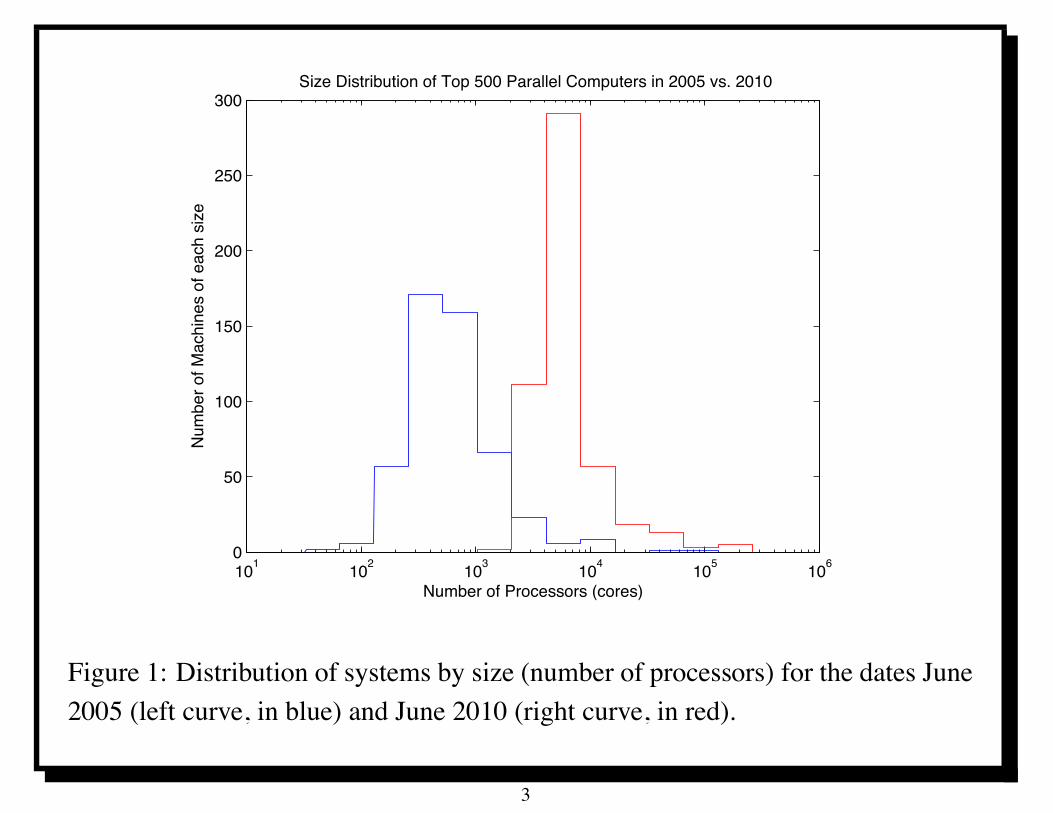
The Top 500 web page tracks the evolution of supercomputingworldwide.It has a database of the 500 most powerful supercomputers aroundthe world over the last two decades.The five hundred most powerful supercomputers in the world havebeen parallel computers for about two decades.Moreover, the number of processors (cores) per system continues toincrease.The following figure shows the distribution of systems by size(number of processors) for the dates June 2005 (left curve, in blue)and June 2010 (right curve, in red).This clearly shows a trend towards utilization of larger numbers ofprocessors.
2
101 102 103 104 105 1060
50
100
150
200
250
300Size Distribution of Top 500 Parallel Computers in 2005 vs. 2010
Number of Processors (cores)
Num
ber o
f Mac
hine
s of
eac
h siz
e
Figure 1: Distribution of systems by size (number of processors) for the dates June2005 (left curve, in blue) and June 2010 (right curve, in red).
3
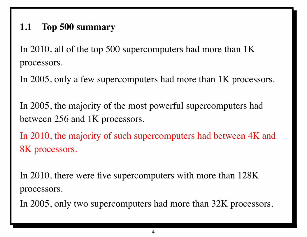
1.1 Top 500 summary
In 2010, all of the top 500 supercomputers had more than 1Kprocessors.
In 2005, only a few supercomputers had more than 1K processors.
In 2005, the majority of the most powerful supercomputers hadbetween 256 and 1K processors.
In 2010, the majority of such supercomputers had between 4K and8K processors.
In 2010, there were five supercomputers with more than 128Kprocessors.In 2005, only two supercomputers had more than 32K processors.
4
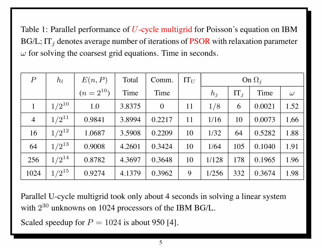
Table 1: Parallel performance of U -cycle multigrid for Poisson’s equation on IBMBG/L; ITj denotes average number of iterations of PSOR with relaxation parameter! for solving the coarsest grid equations. Time in seconds.
P hl E(n,P ) Total Comm. ITU On !j
(n = 210) Time Time hj ITj Time !
1 1/210 1.0 3.8375 0 11 1/8 6 0.0021 1.52
4 1/211 0.9841 3.8994 0.2217 11 1/16 10 0.0073 1.66
16 1/212 1.0687 3.5908 0.2209 10 1/32 64 0.5282 1.88
64 1/213 0.9008 4.2601 0.3424 10 1/64 105 0.1040 1.91
256 1/214 0.8782 4.3697 0.3648 10 1/128 178 0.1965 1.96
1024 1/215 0.9274 4.1379 0.3962 9 1/256 332 0.3674 1.98
Parallel U-cycle multigrid took only about 4 seconds in solving a linear systemwith 230 unknowns on 1024 processors of the IBM BG/L.
Scaled speedup for P = 1024 is about 950 [4].
5
1.2 HPC application: employment
Post Doctoral Fellow in Parallel Scalable Algorithms and Software
This position is part of a research program to extend the Uintah software(www.uintah.utah.edu) as applied to challenging problems in combustion and energy topetascale and beyond using novel algorithmic and software approaches. Uintah is ascalable, highly parallel framework designed to simulate complex fluid-structureinteraction problems, with a clear partition between the parallel framework and thenumerical algorithms.
The postdoc will be expected to perform algorithmic and parallel computing research tohelp Uintah scale to beyond 98K cores. The work is projected to last for three years andwill involve research, analysis, and continuing development of scalable adaptive algorithmsin the areas such as adaptive meshing and linear solvers in the context of combustion andenergy-related problems combined with implementation and scaling studies using theUintah code base.
The requirement is for an individual with highly developed algorithmic and C++programming skills who must have experience in developing parallel algorithms andsoftware. Familiarity with adaptive grid and/or linear solver techniques is desirable. Pleasecontact Martin Berzins ([email protected]) for further information. [26 Dec 2010]
6
2 What is Parallel Computing?
Application of two or more processing units to solve asingle problem.
Practical objective: scale to thousands of processors.Requires some form of synchronization so that the value in memoryis accessed when it is valid.
Can be achieved in various ways: messages, semaphores.
Different languages use different approaches.
Different architectures support different techniques.
Ultimately, parallel algorithms are the central issue.Performance analysis supports development process.
7
The secrets to parallel computing
Figure 2: Depiction of a critical section, cover of Scientific Parallel Computing, byScott, Clark and Bagheri, Princeton Univ. Press, 2005 [16].
8
Architecture Algorithms
ParallelComputing
Languages
APPLICATIONS
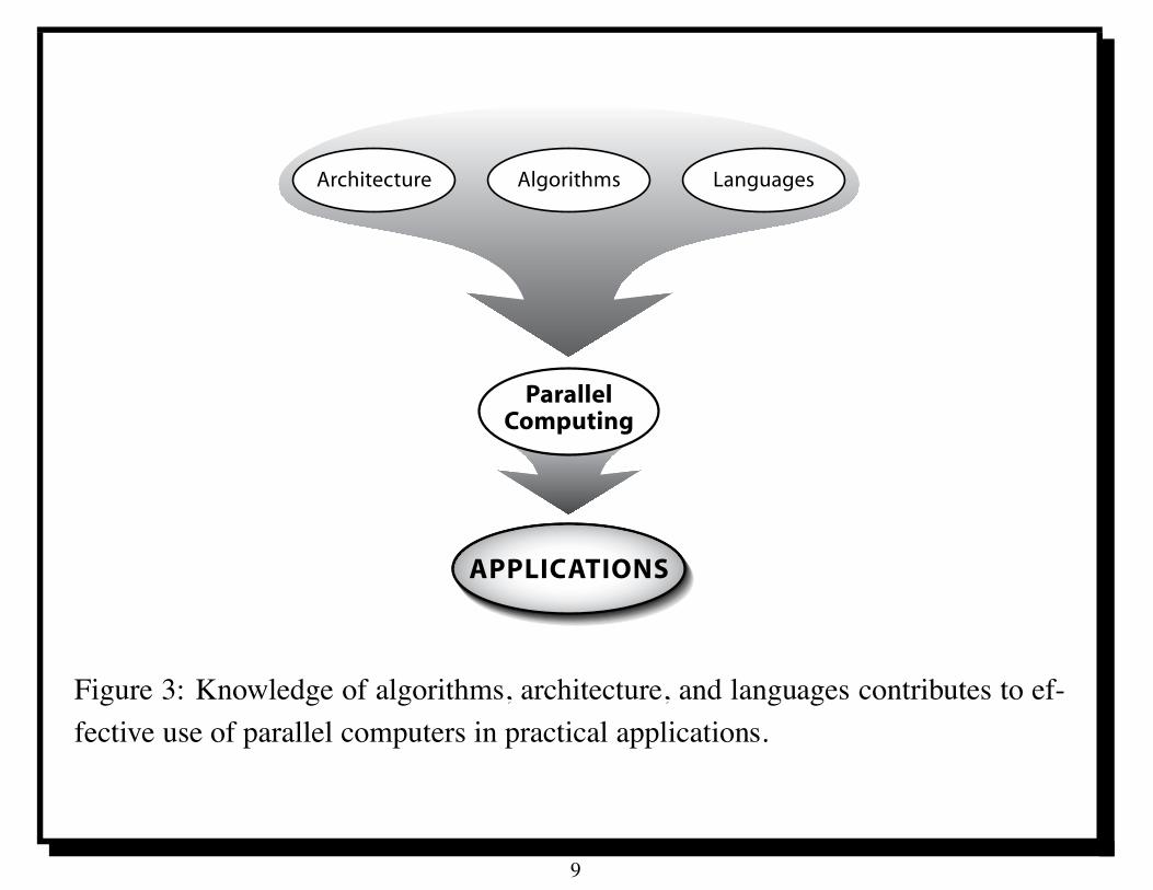
Figure 3: Knowledge of algorithms, architecture, and languages contributes to ef-fective use of parallel computers in practical applications.
9
3 Plan for the course
Basic notions relating to performance
• Influence of memory and load balancing
Performance measures
• Speedup, Efficiency, Amdhahl’s Law, and Scalability
PMS notation and computer architecture
• Influence of memory systems on performance
Dependence analysis (loop-carried dependences)
Basic algorithms: linear systems
• Scalable algorithms for sparse triangular systems
Novel algorithms: parallelization in time
• Scalable algorithms for solving ODE’s
10
4 Performance
In scientific computing, performance is a constraint,not an objective.Definition 4.1 A Craya is 109 floating-point operations per second(one floating-point operation per nanosecond), the level ofperformance being achieved by a single processor at SeymourCray’s untimely death.
aThe development of the first “supercomputers” was largely the result of effortslead by Seymour Cray (1925-1996). Seymour Cray earned a BS in engineeringfrom the University of Minnesota in 1950. He co-founded Control Data Corpora-tion (CDC) in 1957; the CDC 6600 is the primary candidate for the title of “firstsupercomputer.” The series of supercomputers bearing Cray’s name were producedby Cray Research. Started in 1972, this company was headquartered in Seymour’sboyhood home, Chippewa Falls, Wisconsin, also home of the Jacob LeinenkugelBrewing Co.
11
4.1 Memory effects
Memory access is the critical issue in high-performance computing.Definition 4.2 The work/memory ratio "WM: number of floating-point operationsdivided by number of memory locations referenced (either reads or writes).
A look at a book of mathematical tables tells us that#
4= 1 ! 1
3+
1
5! 1
7+
1
9! 1
11+
1
13! 1
15+ · · · (4.1)
Slowly converging series good example for studying basic operation of computingthe sum of a series of numbers:
A =N!
i=1
ai. (4.2)
Computation of A in equation (4.2) requires N ! 1 floating-point additions andinvolves N + 1 memory locations: one for A and n for the ai’s.
Therefore, work/memory ratio for this algorithm is "WM = (N ! 1)/(N + 1) " 1
for large N .
12
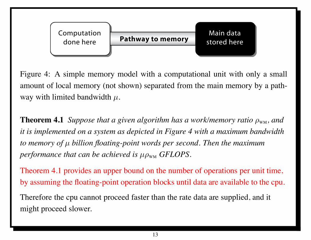
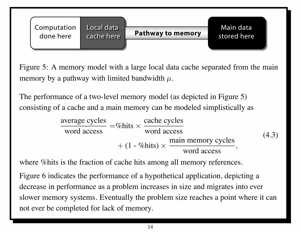
Computationdone here Pathway to memory
Main datastored here
Figure 4: A simple memory model with a computational unit with only a smallamount of local memory (not shown) separated from the main memory by a path-way with limited bandwidth µ.
Theorem 4.1 Suppose that a given algorithm has a work/memory ratio "WM, andit is implemented on a system as depicted in Figure 4 with a maximum bandwidthto memory of µ billion floating-point words per second. Then the maximumperformance that can be achieved is µ"WM GFLOPS.
Theorem 4.1 provides an upper bound on the number of operations per unit time,by assuming the floating-point operation blocks until data are available to the cpu.
Therefore the cpu cannot proceed faster than the rate data are supplied, and itmight proceed slower.
13
Computationdone here Pathway to memory
Main datastored here
Local data cache here
Local data cache here
Figure 5: A memory model with a large local data cache separated from the mainmemory by a pathway with limited bandwidth µ.
The performance of a two-level memory model (as depicted in Figure 5)consisting of a cache and a main memory can be modeled simplistically as
average cyclesword access
=%hits # cache cyclesword access
+ (1 - %hits) # main memory cyclesword access
,
(4.3)
where %hits is the fraction of cache hits among all memory references.
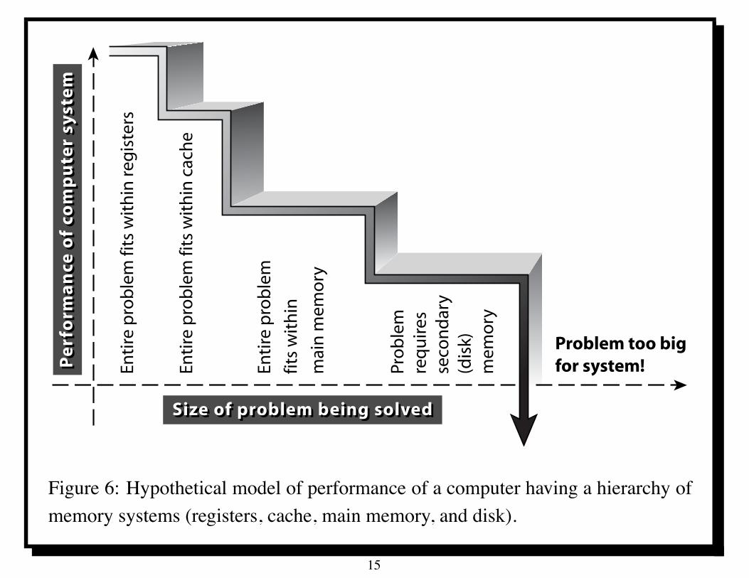
Figure 6 indicates the performance of a hypothetical application, depicting adecrease in performance as a problem increases in size and migrates into everslower memory systems. Eventually the problem size reaches a point where it cannot ever be completed for lack of memory.
14
Enti
re p
rob
lem
fit
s w
ith
in r
egis
ters
Enti
re p
rob
lem
fit
s w
ith
in c
ach
e
Enti
re p
rob
lem
fits
wit
hin
mai
n m
emo
ry
Pro
ble
mre
qu
ires
seco
nd
ary
(dis
k)m
emo
ry
Problem too bigfor system!P
erf
orm
an
ce o
f co
mp
ute
r sy
ste
m
Size of problem being solved
Pe
rfo
rma
nce
of
com
pu
ter
syst
em
Size of problem being solved
Figure 6: Hypothetical model of performance of a computer having a hierarchy ofmemory systems (registers, cache, main memory, and disk).
15
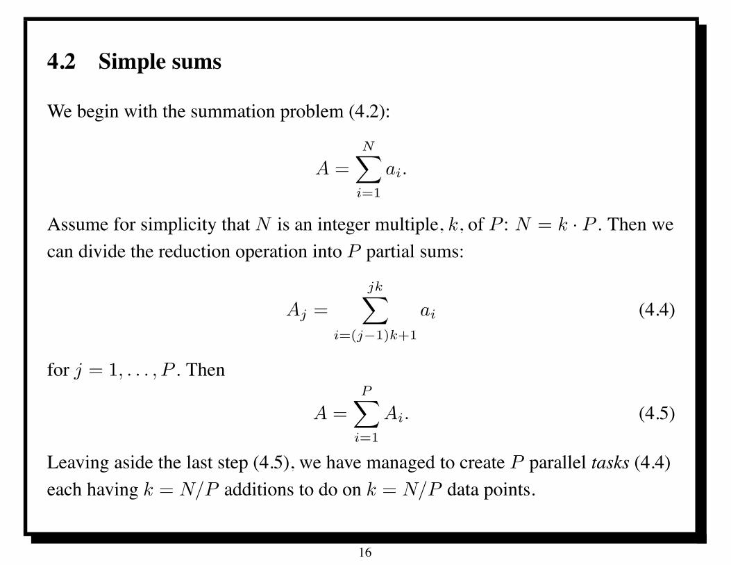
4.2 Simple sums
We begin with the summation problem (4.2):
A =N!
i=1
ai.
Assume for simplicity that N is an integer multiple, k, of P : N = k · P . Then wecan divide the reduction operation into P partial sums:
Aj =jk!
i=(j!1)k+1
ai (4.4)
for j = 1, . . . , P . Then
A =P!
i=1
Ai. (4.5)
Leaving aside the last step (4.5), we have managed to create P parallel tasks (4.4)each having k = N/P additions to do on k = N/P data points.
16
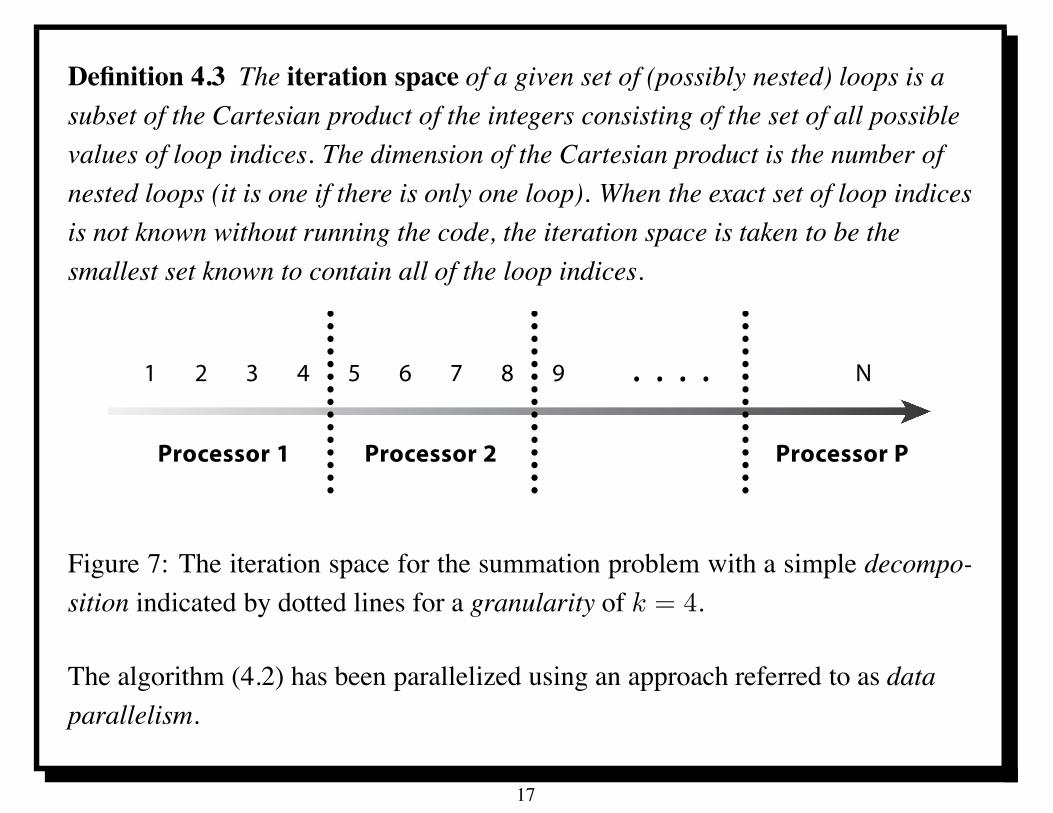
Definition 4.3 The iteration space of a given set of (possibly nested) loops is asubset of the Cartesian product of the integers consisting of the set of all possiblevalues of loop indices. The dimension of the Cartesian product is the number ofnested loops (it is one if there is only one loop). When the exact set of loop indicesis not known without running the code, the iteration space is taken to be thesmallest set known to contain all of the loop indices.
Processor 1 Processor 2 Processor P
1 2 3 4 5 6 7 8 9 . . . . N
Figure 7: The iteration space for the summation problem with a simple decompo-sition indicated by dotted lines for a granularity of k = 4.
The algorithm (4.2) has been parallelized using an approach referred to as dataparallelism.
17
4.3 Load balancing
Figure 7 depicts graphically the iteration space for the summation problem (4.2)parallelized using the decomposition in (4.4).
If the work is not distributed equally, then one processor may end up taking longerthan the others.
Definition 4.4 Suppose that a set of parallel tasks (indexed by i = 1, . . . , P )execute in an amount of time ti. Define the average execution time
ave {ti : 1 $ i $ P} :=1
P
!
1"i"P
ti. (4.6)
The load balance $ of this set of parallel tasks is
$ :=ave {ti : 1 $ i $ P}max {ti : 1 $ i $ P} . (4.7)
A set of tasks is said to be load balanced if $ is close to one.
18
4.4 About the definition
The amount the load balance $ differs from the ideal case $ = 1 measures therelative difference between the longest task and the average task:
1 ! $ =max {ti : 1 $ i $ P}! ave {ti : 1 $ i $ P}
max {ti : 1 $ i $ P} . (4.8)
Note that we have compared the average time with the maximum time, not theminimum time.
The relevance of this will become clearer in Section 4.5 and Section 7.5.
Have defined load balance in terms of time of execution instead of amount ofcomputational work to be done.
Performance (Definition 4.1) need not be the same for different tasks, and the costof the computation is proportional to the time it takes, not to how manyfloating-point operations get done.
Often try to achieve load balance by balancing the amount of work to be done, butdynamic load balancing is often needed.
19
4.5 Minimum run time is not relevant for load balance
Optimal run time can be achieved when one processor does nothing.Suppose P processors are used to sum n = (P ! 1)k + 1 numbers.
All but one processor does k ! 1 floating point operations involving k summands.
When k $ P , the fastest possible execution time involves at least one processordoing k ! 1 floating point operations with k summands.
Proof: If less than k summands are assigned to all processors, then at most(k ! 1)P summands would have been assigned. This means that the number ofunassigned summands is at least
k(P ! 1) + 1 ! (k ! 1)P = P ! k + 1.
Since k $ P , at least one summand is left out, and this would not be a validalgorithm.
Therefore, the fastest possible execution time involves at least one processordoing k ! 1 floating point operations with k summands.
20
5 Limits to Parallel Performance
Parallel performance is more complex than sequential performance in many ways:first and foremost, it is more difficult to achieve good parallel performance, but itis also more difficult to predict and even to measure.
This is due largely to the fact that essentially independent computers arecooperating on a single task.
With simple (low-performance) sequential processors, it has been possible topredict sequential performance based on a textual analysis of code or amathematical description of an algorithm, by counting the number of basicoperations.
With parallel computation, other factors become critical, such as
• synchronization,
• load balance, and
• communication costs.
21
5.1 Limits to Parallel Performance: outline
There are significant limits to utilizing parallel computers efficiently.
Perhaps the most well known caveat is Amdahl’s Law.
This is a statement about the potential speed-up achievable with a number ofparallel processors.
Based on the notion of speed-up, one can define a notion of parallel efficiency.
The basic notion of speed-up as addressed in Amdahl’s law relates primarily toproblems of fixed size.
In many cases, one deals with problems of varying size, characterized by someparameter usually related to the size of the data set.
In this case, it may be appropriate to use large computers only for large problems.
The notion of scalability relates to whether a given algorithm or code can be usedefficiently on a range of problem sizes when using an appropriately chosennumber of processors.
22
5.2 Summation example
Consider the simple parallel summation algorithm to compute"N
i=1 ai.
Each processor computes a partial sum
Aj =
ej!
i=sj
ai.
Consider a collection of individual workstations or personal computers connectedby some broadcast medium like Ethernet.
Time of execution on each processor separately should be proportional to N/P
assuming that N is divisible by P .
The constant of proportionality will depend on properties of the individualprocessors and their own memory systems (which we assume are large enough tohold the required data).
For the sake of simplicity, we will normalize so that our unit of time is such thatthis constant of proportionality is one. Thus the time of execution is exactly N/P .
23
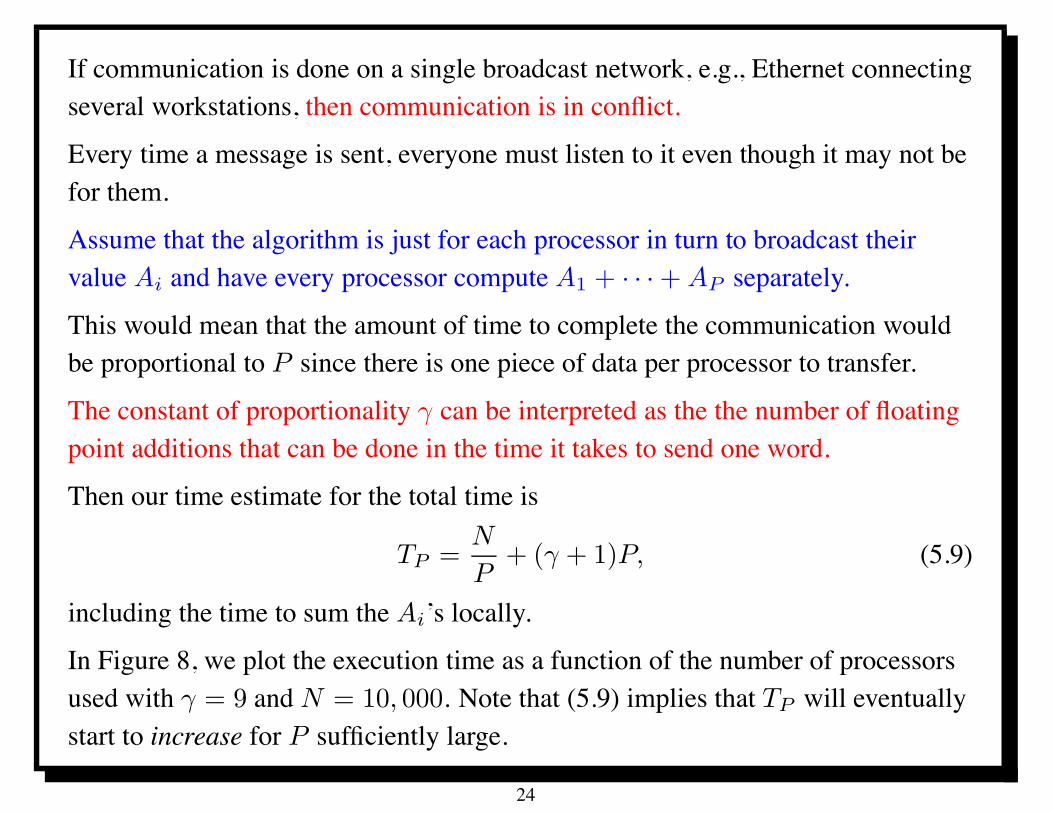
If communication is done on a single broadcast network, e.g., Ethernet connectingseveral workstations, then communication is in conflict.
Every time a message is sent, everyone must listen to it even though it may not befor them.
Assume that the algorithm is just for each processor in turn to broadcast theirvalue Ai and have every processor compute A1 + · · · + AP separately.
This would mean that the amount of time to complete the communication wouldbe proportional to P since there is one piece of data per processor to transfer.
The constant of proportionality % can be interpreted as the the number of floatingpoint additions that can be done in the time it takes to send one word.
Then our time estimate for the total time is
TP =N
P+ (% + 1)P, (5.9)
including the time to sum the Ai’s locally.
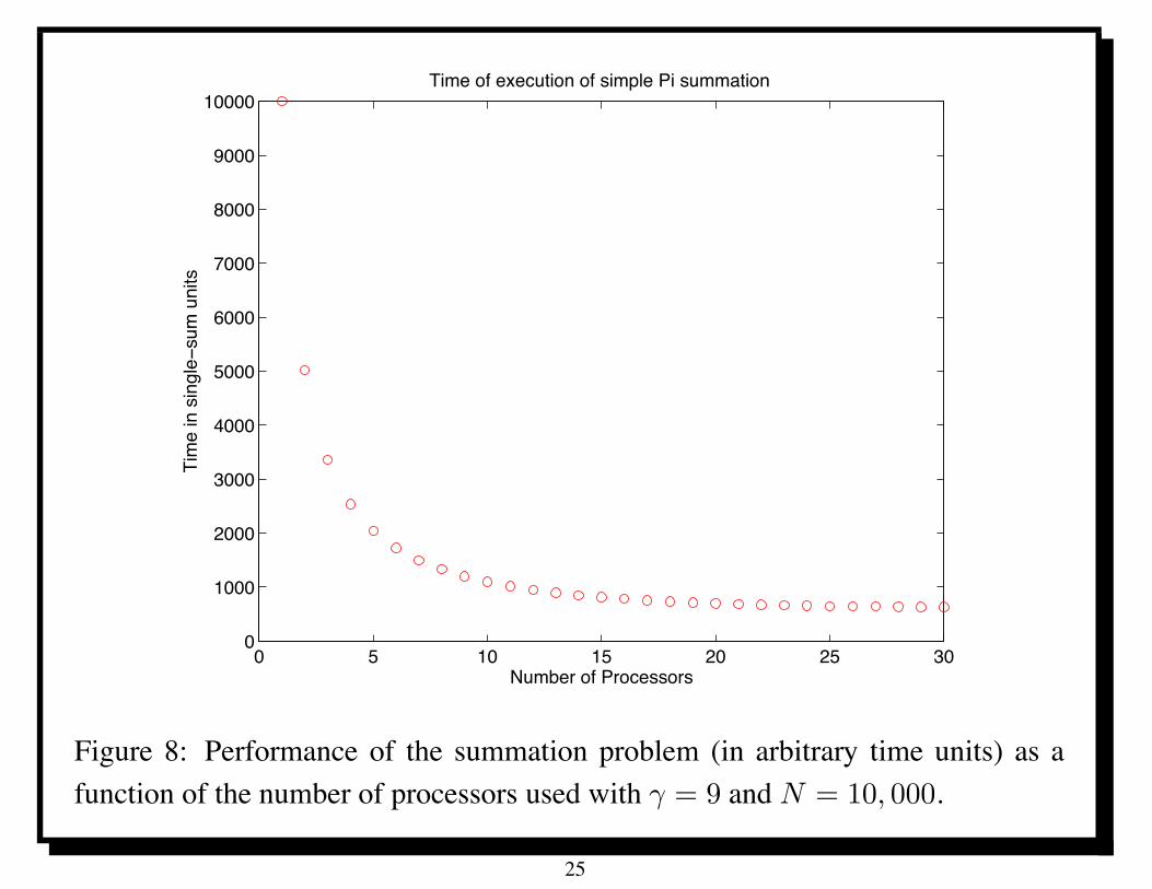
In Figure 8, we plot the execution time as a function of the number of processorsused with % = 9 and N = 10, 000. Note that (5.9) implies that TP will eventuallystart to increase for P sufficiently large.
24
0 5 10 15 20 25 300
1000
2000
3000
4000
5000
6000
7000
8000
9000
10000Time of execution of simple Pi summation
Number of Processors
Tim
e in
sin
gle−
sum
uni
ts
Figure 8: Performance of the summation problem (in arbitrary time units) as afunction of the number of processors used with % = 9 and N = 10, 000.
25
6 Performance measures
This plot in Figure 8 is very forgiving; gives the illusion of positive achievementas long as it decreases.
A more critical way to evaluate the behavior of our parallelization is to considerthe speed-up that has been achieved.
6.1 Speed-up
Definition 6.1 The speed-up, SP , using P processors is defined to be the ratio ofthe sequential and parallel execution times
SP =T1
TP. (6.10)
More precisely, T1 should be the time of execution of the best available sequentialsolution of the problem, and TP should be the time of execution of the parallelsolution of the problem on P processors.
26
The speed-up for the performance in (5.9) is
SP =N
NP + (% + 1)P
=P
1 + (% + 1)P 2/N. (6.11)
We refer to the case SP " P as linear speed-up or perfect speed-up.
In the very fortunate case that SP > P we call it super-linear speed-up, orperhaps more grammatically correctly, supra-linear speed-up.
In practice, SP can sometimes exceed P due to the effective improvement ofindividual processor performance due to decreasing local data size.
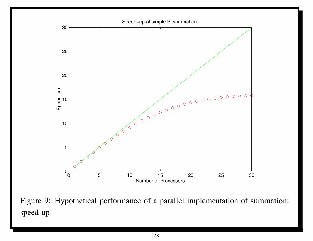
Figure 9 shows speed-up plot corresponding to the execution times in Figure 8.
This is a more demanding view of performance as it emphasizes the deviationfrom the ideal linear speed-up indicated by the straight line of slope one.
In Figure 8, we saw something bad (execution time) decreasing as a function ofthe number of processors, so that gave us a positive feeling.
But now we see something good (speed-up) beginning to flag, so we begin to bemore skeptical.
27
0 5 10 15 20 25 300
5
10
15
20
25
30Speed−up of simple Pi summation
Number of Processors
Spee
d−up
Figure 9: Hypothetical performance of a parallel implementation of summation:speed-up.
28
Often, SP will be significantly less than P , and there is no guarantee that it will begreater than one!
If SP < 1, it should be called “slow-down” not speed-up.
SP will not increase indefinitely in all cases. More likely, as in the example (5.9),it will reach a maximum and then decrease.
Since SP is inversely proportional to the execution time TP , the maximum of SP
will occur at the minimum of TP .
In some cases, it may not be possible to run a problem on one just processor dueto memory or time constraints.
In this case, we may want instead to define speed-up with respect to the smallestnumber P # of processors for which the problem will run. Define
SP !
P =TP !
TP(6.12)
to be the corresponding relative speed-up in this case for P % P #. We expectSP !
P " P/P # in the ideal case.
29
6.2 Parallel efficiency
The most demanding view of performance data compares observed speed-up withideal speed-up, obtaining a measure of efficiency.
Definition 6.2 The parallel efficiency, EP , using P processors is defined to bethe ratio of the speed-up and P , that is
EP :=SP
P=
T1
PTP, (6.13)
where T1 is time of execution of best sequential solution of the problem, and TP istime of execution of the parallel solution with P processors.
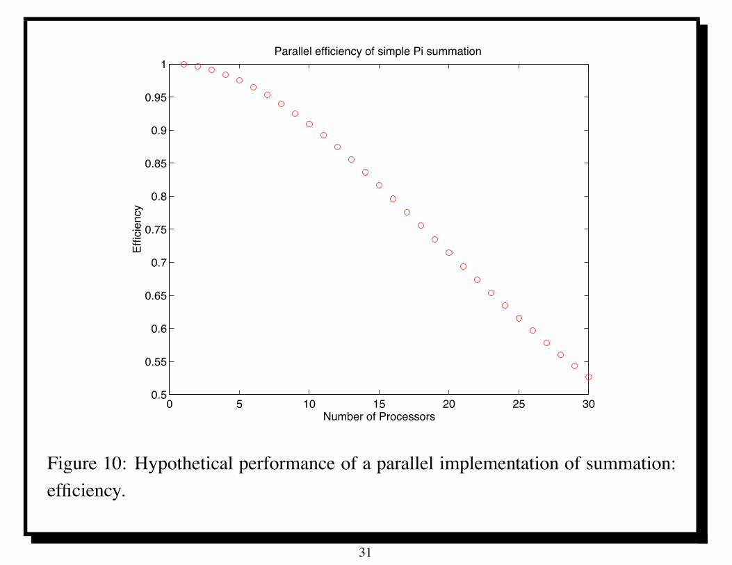
Figure 10 shows parallel efficiency for performance data in Figure 8.
Now something good (efficiency) is going down; now we are not so pleased.
However, the parallel efficiency of a code is critical to the economic viability ofusing it on a given number of processors.
The efficiency provides a measure of the relative utilization of the resources of aparallel computer, as follows.
30
0 5 10 15 20 25 300.5
0.55
0.6
0.65
0.7
0.75
0.8
0.85
0.9
0.95
1Parallel efficiency of simple Pi summation
Number of Processors
Effic
ienc
y
Figure 10: Hypothetical performance of a parallel implementation of summation:efficiency.
31
6.3 Efficiency and cost
Suppose that you have to pay the same rate " for time for each processor used,without regard for problem size or total number of processors used.
This very simple charging algorithm simplifies our argument.
The cost C1 of using one processor to do a job is
C1 = "T1
(" is the cost per unit time) whereas the cost CP of using P processors is
CP = "TP P ="T1
EP=
C1
EP. (6.14)
Thus the cost of using P processors is related to the sequential cost by a simplefactor of 1/EP .
A more realistic measure of the cost of using a parallel computer would be tocompare with the cost on an independent sequential computer.
32
7 Limits to performance
There are many things that can limit parallel performance. Here we present somekey results that quantify some of these effects.
7.1 Amdahl’s Law
Suppose that a particular code takes time T1 to execute on one processor and thatthere is a sequential fraction f of this code that cannot be (or has not been)parallelized (for whatever reason).
Amdahl’s Law assumes that, no matter how many processors P are used, thesequential part of the code will require at least fT1 time to complete.
The remainder of the code, by assumption, takes (1! f)T1 time to execute on oneprocessor.
Amdahl’s Law assumes that this part of the code will require at least (1! f)T1/P
time to execute on P processors.
33
Combining these two time estimates, the time TP to execute this code using P
processors is bounded below by the sum of the sequential fraction fT1 of theexecution time and the remaining fraction (1 ! f)T1 divided by P :
TP % fT1 +(1 ! f)T1
P. (7.15)
Combining (7.15) and (6.10), we obtain Amdahl’s Law:
SP $ 1
f + (1 ! f)/P. (7.16)
Even with an infinite number of processors, the speed-up could not exceed
SP $ 1
f. (7.17)
This weaker statement is also sometimes referred to as Amdahl’s Law. It says thatthe ratio of the parallel and sequential execution times cannot be less that thesequential fraction of the code:
TP
T1% f. (7.18)
34
7.2 But wait there’s more
Other factors can limit parallel performance in addition to the sequential fractionof a code.
This is why inequalities are used in (7.15) and (7.16).
In all the examples we have seen, there is some communication that must go onbetween processors which would not occur (or be simpler) in the sequential case.
Thus we may assume that communication will add some additional overhead, as ageneral rule.
This will arise in a variety of ways (through message latency, network or buscontention, or network bandwidth limitations) depending on particulararchitectural details of the computer, but it will almost always appear in someguise when P > 1.
35
7.3 But wait there’s more
Lack of synchronization also limits parallel performance
Some parts of a parallel computation cannot be initiated until other parts arecompleted. Some processors may be forced to sit idle waiting for others tocomplete required tasks. In this time, no useful computation is done.
This means that the “parallel” computation time will not be the sequential timedivided by P even if there is no sequential fraction to the code and thecommunication volume is minimal.
A frequent cause of idleness is a lack of load balance (Section 7.5) in one part ofthe computation which is followed by some communication.
The assumptions here do not take into account the fact that the individualprocessor performance may increase. This can and does allow speed-up to exceedthe theoretical linear limit in practical calculations [3]. Amdahl’s law assumesuniform processor behavior, which is a reasonable approximation. However,individual processor performance is becoming increasingly data dependent, socaution should be exercised in using the model.
36
7.4 Efficiency and Amdhahl’s Law
Amdahl’s Law implies that that the parallel efficiency (Definition 6.2) is boundedby
EP $ 1
1 + (P ! 1)f. (7.19)
When the quantity (P ! 1)f is small, expanding the quotient implies that EP
decreases likeEP " 1 ! (P ! 1)f. (7.20)
Thus f can be interpreted as the slope of the efficiency curve, EP , as a function ofP , near the point P = 1.
37
7.5 Load balance and efficiency
In the derivation of Amdahl’s Law we assumed the best case for estimatingparallel performance, namely that the parallel work could be perfectly divided intoP parts. This is the case of perfect load balance (Definition 1.5.7), where loadrefers to a measure of the amount of work done by each individual processor.
Recall that the definition of load balance (Definition 1.5.7) is stated in terms of thetimes ti for each processor to do its part of the calculation. The calculation is loadbalanced when all the ti’s are approximately the same. The parallel executiontime can be defined simply in terms of the ti’s as follows:
TP = max {ti : 1 $ i $ P} . (7.21)
It is reasonable to assume that
T1 $!
1"i"P
ti. (7.22)
If not, then the parallel execution could provide a faster sequential execution byexecuting each separate part in sequence.
38
Applying the definition of efficiency (Definition 6.2) and (7.21) and (7.22), wefind
EP =T1
PTP$
"1"i"P ti
P max {ti : 1 $ i $ P}=
ave {ti : 1 $ i $ P}max {ti : 1 $ i $ P}
(7.23)
where we recall the definition (1.5.3) of ave{ti : 1 $ i $ P}. Thus the ratio ofthe average time on each processor to the maximum time on each processor,which we used as the definition of load balance (Definition 4.4), gives an upperbound on the efficiency of a calculation. We state this important result as thefollowing Theorem.
Theorem 7.1 Let ti denote the time for the i-th processor to do its part of thecalculation. Suppose that (7.22) holds. Then the efficiency of the calculation cannever exceed the load balance:
EP $ $ :=ave {ti : 1 $ i $ P}max {ti : 1 $ i $ P} (7.24)
where the numerator was defined in (1.5.3) and $ denotes the load balance(Definition 4.4).
39
It is permissible to combine the bounds (7.19) (Amdahl’s Law for parallelefficiency) and (7.24). The latter applies to trivially parallel tasks where thesequential fraction f is zero. The parallel speed-up and efficiency of twosuccessive tasks can be estimated as follows from the corresponding speed-up andefficiency of the separate tasks. Suppose that T a
· and T b· denote the times of
execution of the two separate tasks, labelled “a” and “b” respectively. Thus T a1
denotes the sequential time of task “a”, T bP denotes the parallel time of task “b”,
etc. It is reasonable to assume that the sequential time T a+b1 of the combined tasks
“a + b” is the sum of the sequential times of the separate parts:
T a+b1 = T a
1 + T b1 . (7.25)
On the other hand, it would be prudent only to assume that the parallel time T a+b1
of the combined tasks “a + b” is not less than the sum of the parallel times of theseparate parts:
T a+bP % T a
P + T bP (7.26)
as there could be additional contributions to parallel execution time due tocommunication or synchronization.
40
Then one can show by simple algebra that the corresponding speed-up Sa+bP of
the combined tasks satisfies
Sa+bP $
#&
SaP
+1 ! &
SbP
$!1
(7.27)
where& :=
T a1
T a1 + T b
1
. (7.28)
Since efficiency is just speed-up divided by P , we similarly have
Ea+bP $
#&
EaP
+1 ! &
EbP
$!1
. (7.29)
41
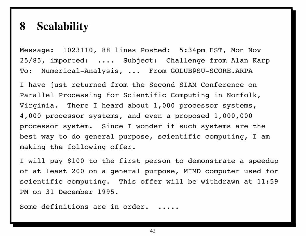
8 Scalability
Message: 1023110, 88 lines Posted: 5:34pm EST, Mon Nov25/85, imported: .... Subject: Challenge from Alan KarpTo: Numerical-Analysis, ... From [email protected]
I have just returned from the Second SIAM Conference onParallel Processing for Scientific Computing in Norfolk,Virginia. There I heard about 1,000 processor systems,4,000 processor systems, and even a proposed 1,000,000processor system. Since I wonder if such systems are thebest way to do general purpose, scientific computing, I ammaking the following offer.
I will pay $100 to the first person to demonstrate a speedupof at least 200 on a general purpose, MIMD computer used forscientific computing. This offer will be withdrawn at 11:59PM on 31 December 1995.
Some definitions are in order. .....
42
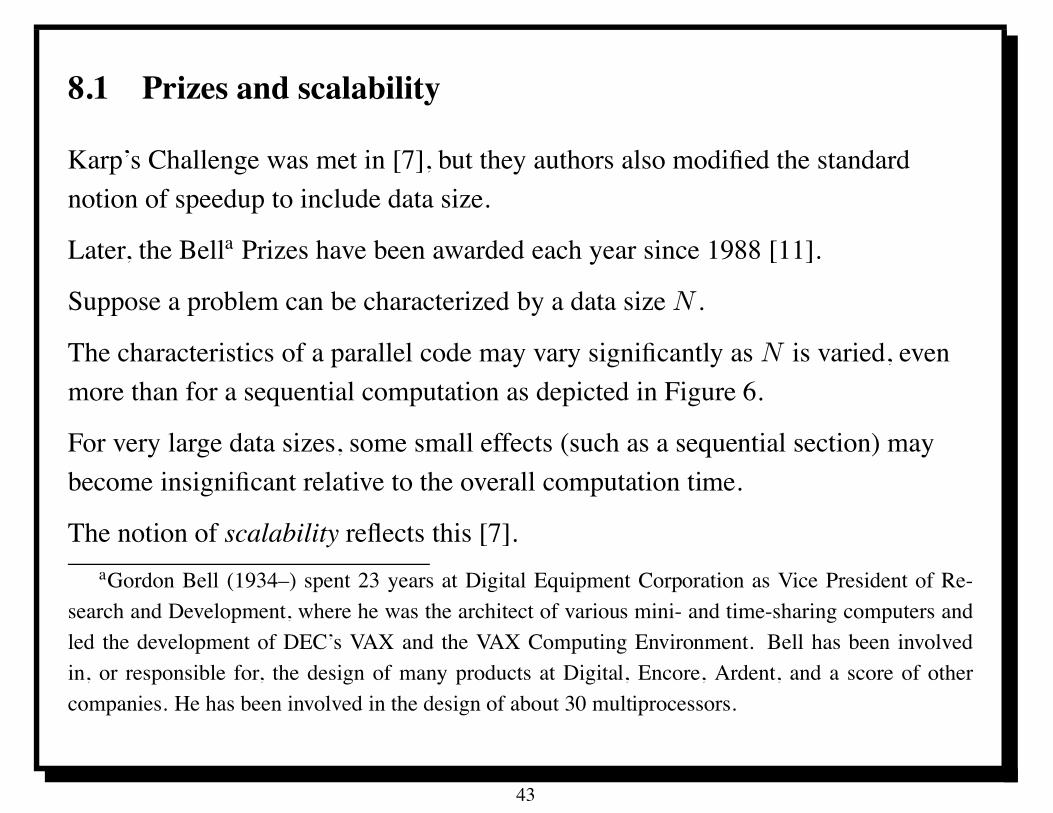
8.1 Prizes and scalability
Karp’s Challenge was met in [7], but they authors also modified the standardnotion of speedup to include data size.
Later, the Bella Prizes have been awarded each year since 1988 [11].
Suppose a problem can be characterized by a data size N .
The characteristics of a parallel code may vary significantly as N is varied, evenmore than for a sequential computation as depicted in Figure 6.
For very large data sizes, some small effects (such as a sequential section) maybecome insignificant relative to the overall computation time.
The notion of scalability reflects this [7].aGordon Bell (1934–) spent 23 years at Digital Equipment Corporation as Vice President of Re-
search and Development, where he was the architect of various mini- and time-sharing computers andled the development of DEC’s VAX and the VAX Computing Environment. Bell has been involvedin, or responsible for, the design of many products at Digital, Encore, Ardent, and a score of othercompanies. He has been involved in the design of about 30 multiprocessors.
43
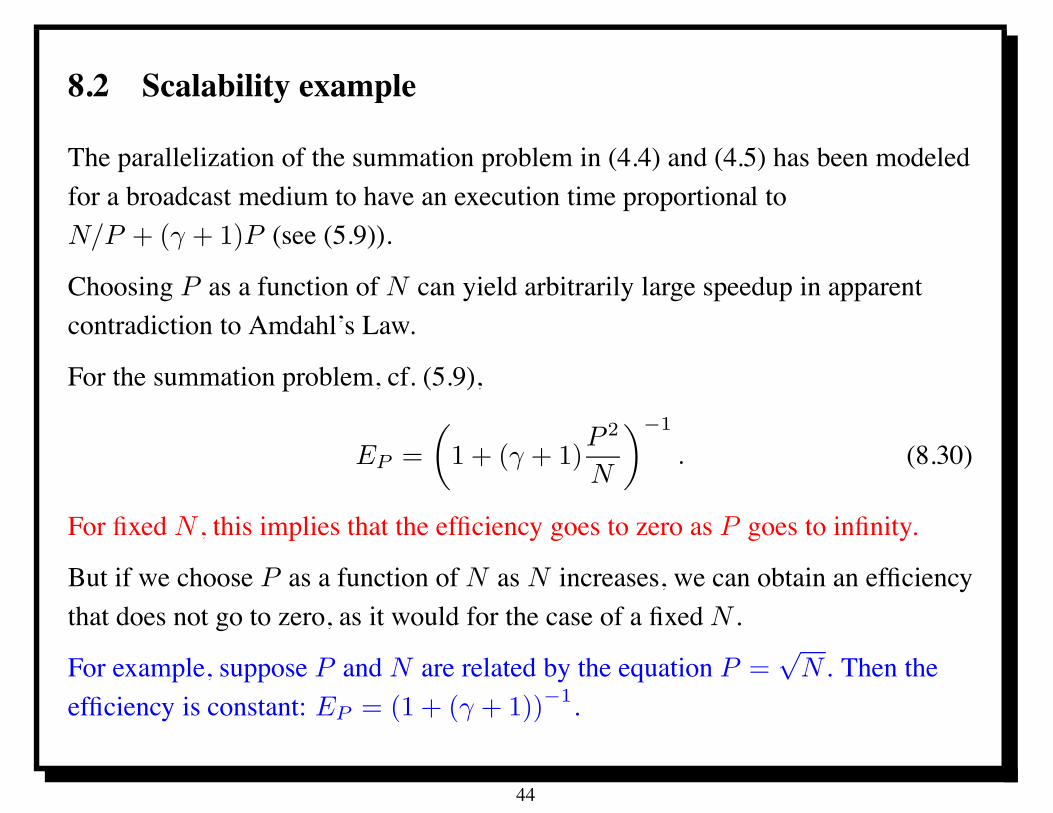
8.2 Scalability example
The parallelization of the summation problem in (4.4) and (4.5) has been modeledfor a broadcast medium to have an execution time proportional toN/P + (% + 1)P (see (5.9)).
Choosing P as a function of N can yield arbitrarily large speedup in apparentcontradiction to Amdahl’s Law.
For the summation problem, cf. (5.9),
EP =
#1 + (% + 1)
P 2
N
$!1
. (8.30)
For fixed N , this implies that the efficiency goes to zero as P goes to infinity.
But if we choose P as a function of N as N increases, we can obtain an efficiencythat does not go to zero, as it would for the case of a fixed N .
For example, suppose P and N are related by the equation P =&
N . Then theefficiency is constant: EP = (1 + (% + 1))!1.
44
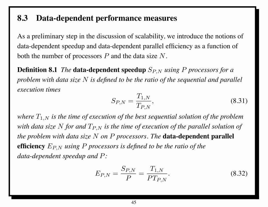
8.3 Data-dependent performance measures
As a preliminary step in the discussion of scalability, we introduce the notions ofdata-dependent speedup and data-dependent parallel efficiency as a function ofboth the number of processors P and the data size N .
Definition 8.1 The data-dependent speedup SP,N using P processors for aproblem with data size N is defined to be the ratio of the sequential and parallelexecution times
SP,N =T1,N
TP,N, (8.31)
where T1,N is the time of execution of the best sequential solution of the problemwith data size N for and TP,N is the time of execution of the parallel solution ofthe problem with data size N on P processors. The data-dependent parallelefficiency EP,N using P processors is defined to be the ratio of thedata-dependent speedup and P :
EP,N =SP,N
P=
T1,N
PTP,N. (8.32)
45
8.4 Scalability definition
Definition 8.2 An algorithm is said to be scalable if there is aminimal efficiency' > 0 such that, given any problem size N , there is a number of processors P (N),which tends to infinity when N tends to infinity, such that the efficiency EP (N),N
remains bounded below by ', that is,
EP (N),N % ' > 0 (8.33)
as N is made arbitrarily large.
The number of processors P (N) chosen for a given data size N is not specified inthis definition, except that it should increase to infinity as N increases.
Practically, often one has a precise choice of P (N) for which we ask whether ornot (8.33) holds, such as the memory-constrained case (8.41) describedsubsequently.
Leads to more restrictive notion of scalability than Definition 8.2.
46
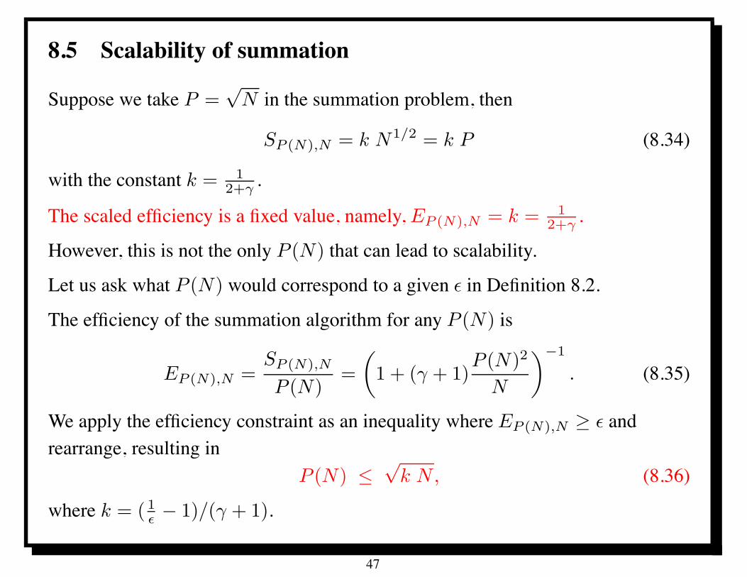
8.5 Scalability of summation
Suppose we take P =&
N in the summation problem, then
SP (N),N = k N1/2 = k P (8.34)
with the constant k = 12+! .
The scaled efficiency is a fixed value, namely, EP (N),N = k = 12+! .
However, this is not the only P (N) that can lead to scalability.
Let us ask what P (N) would correspond to a given ' in Definition 8.2.
The efficiency of the summation algorithm for any P (N) is
EP (N),N =SP (N),N
P (N)=
#1 + (% + 1)
P (N)2
N
$!1
. (8.35)
We apply the efficiency constraint as an inequality where EP (N),N % ' andrearrange, resulting in
P (N) $&
k N, (8.36)
where k = ( 1" ! 1)/(% + 1).
47
8.6 Scalability and Amdahl’s Law
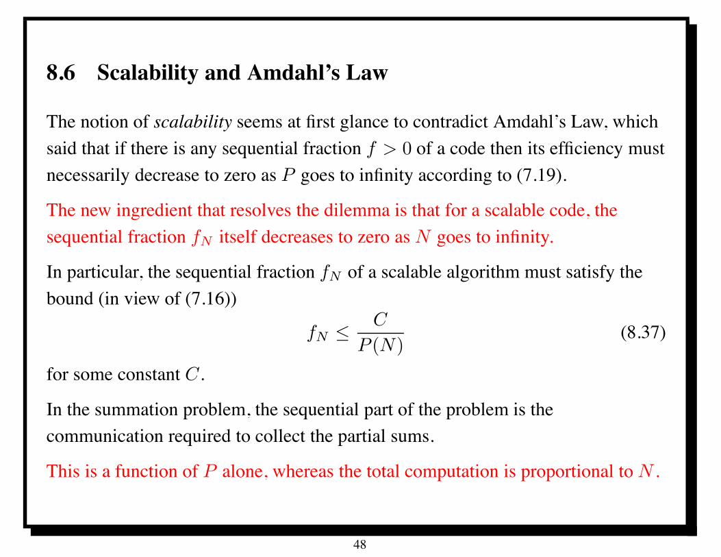
The notion of scalability seems at first glance to contradict Amdahl’s Law, whichsaid that if there is any sequential fraction f > 0 of a code then its efficiency mustnecessarily decrease to zero as P goes to infinity according to (7.19).
The new ingredient that resolves the dilemma is that for a scalable code, thesequential fraction fN itself decreases to zero as N goes to infinity.
In particular, the sequential fraction fN of a scalable algorithm must satisfy thebound (in view of (7.16))
fN $ C
P (N)(8.37)
for some constant C.
In the summation problem, the sequential part of the problem is thecommunication required to collect the partial sums.
This is a function of P alone, whereas the total computation is proportional to N .
48
8.7 Memory limits on performance
The memory M(N, P ) required to implement an algorithm with P processors anddata size N may exceed the physical limits of a particular machine. M(N, P )
denotes the amount of memory required per processor; the total system memoryrequired is thus P times this, i.e., P · M(N, P ).
For a sequential problem, it would be natural to assume that
M(N, 1) $ c0 + c1N
for constants c0 and c1, since N measures the data size.
However, for the parallel case, it is not so easy to say how the local memory sizeM(N, P ) should depend on N (and P ).
It may be possible to divide the memory requirements evenly, leading toM(N, P ) $ c#0 + c#1N/P for possibly different constants c#0 and c#1.
But codes with such an ideal memory behavior may have less than idealperformance.
49
8.8 Memory-constrained scaling
Definition 8.3 An algorithm is said to be scalable with respect to memory if,given any problem size N , there is a number of processors P (N), which tends toinfinity when N tends to infinity, such that the efficiency EP (N),N remainsbounded below by a positive constant as in (8.33), and furthermore
M(N, P (N)) $ MMAX (8.38)
as N is made arbitrarily large, where MMAX is some fixed constant.
Again, the number of processors P (N) chosen for a given data size N has notbeen specified in this definition, except that it should increase indefinitely as N
increases.
We now show that the summation algorithm is not scalable with respect tomemory.
50
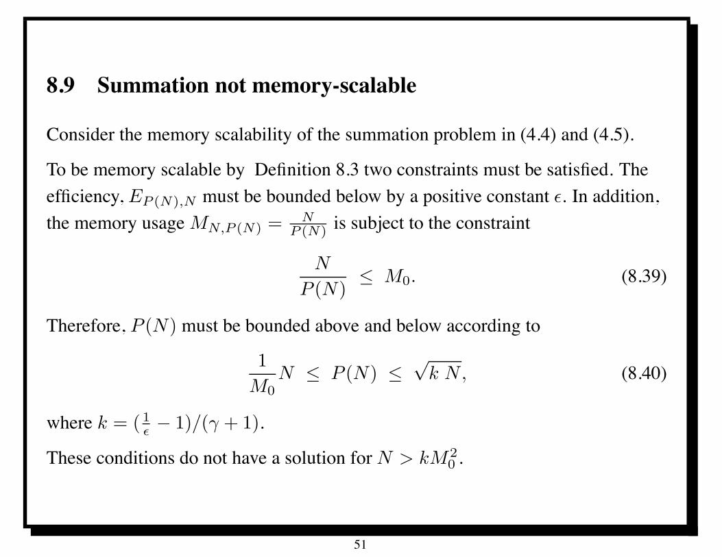
8.9 Summation not memory-scalable
Consider the memory scalability of the summation problem in (4.4) and (4.5).
To be memory scalable by Definition 8.3 two constraints must be satisfied. Theefficiency, EP (N),N must be bounded below by a positive constant '. In addition,the memory usage MN,P (N) = N
P (N) is subject to the constraint
N
P (N)$ M0. (8.39)
Therefore, P (N) must be bounded above and below according to
1
M0N $ P (N) $
&k N, (8.40)
where k = ( 1" ! 1)/(% + 1).
These conditions do not have a solution for N > kM20 .
51
The phrase memory-constrained scaling refers to the performance of analgorithm for a particular amount of memory per processor, independent of N andP . This corresponds to choosing P (N) such that
P (N) = min {P : M(N, P ) $ MMAX} , (8.41)
where MMAX is any constant (not necessarily the same as in Definition 8.3).
Here we are making the simplifying assumption that M(N, P ) is always adecreasing function of P for any given N .
Even if a code is scalable with respect to memory, it may not be scalable for aparticular computer if the constant MMAX in (8.38) is too large for the computer tosupport.
If we take MMAX to be the maximum allowable for a given computer, we can thenask what the efficiency is for P (N) defined by (8.41).
If it is bounded below, then of course the code is scalable with respect to memory.
52
8.10 Weak scaling
Although the definitions of scalability with respect to memory are theoreticallyclear, they are difficult to verify in practice, at least on parallel processors whichfixed memory at each processor.
One might require a single processor with a very large amount of memory to dothe sequential computation to determine T1,N .
One variant of scalability, scaled efficiency or weak scaling, considers thescalability and efficiency with machine resources (memory and processors) as afunction of the problem size.
Scaled efficiency has been used to study the multigrid iterative method for solvinga partial differential equation [17]. The work estimate (and actual execution time)for this algorithm scales linearly with the data size N , i.e.,
T1,N = cN. (8.42)
For ideal performance, we would then expect
TP,N =cN
P. (8.43)
53
8.11 Multigrid scaling
Suppose we are interested in the efficiency of multigrid in the case that we use thesame amount of memory on each processor, independent of the number ofprocessors (cf. the memory-constrained case considered previously). Let n denotethis amount; the total data size is N = nP . Then TP,nP is the time we wouldmeasure for P processors. To compute the efficiency, we would need to know thetime T1,nP which we could not run unless there were a particular processor withnP words of memory. However, (8.42) implies that
T1,nP = PT1,n. (8.44)
Comparing (8.32), we see that
%EP,n :=T1,n
TP,nP(8.45)
provides an estimate of efficiency EP,n in which the amount of memory perprocessor is held fixed. This is a type of memory-constrained scaling, but ofcourse it is not a general definition. For algorithms whose time of execution is notlinear in the data size, a more complex formula would be appropriate.
54
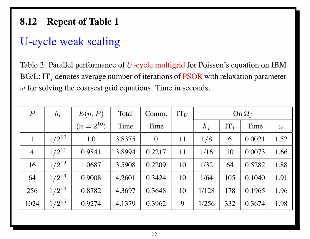
8.12 Repeat of Table 1
U-cycle weak scaling
Table 2: Parallel performance of U -cycle multigrid for Poisson’s equation on IBMBG/L; ITj denotes average number of iterations of PSOR with relaxation parameter! for solving the coarsest grid equations. Time in seconds.
P hl E(n,P ) Total Comm. ITU On !j
(n = 210) Time Time hj ITj Time !
1 1/210 1.0 3.8375 0 11 1/8 6 0.0021 1.52
4 1/211 0.9841 3.8994 0.2217 11 1/16 10 0.0073 1.66
16 1/212 1.0687 3.5908 0.2209 10 1/32 64 0.5282 1.88
64 1/213 0.9008 4.2601 0.3424 10 1/64 105 0.1040 1.91
256 1/214 0.8782 4.3697 0.3648 10 1/128 178 0.1965 1.96
1024 1/215 0.9274 4.1379 0.3962 9 1/256 332 0.3674 1.98
55
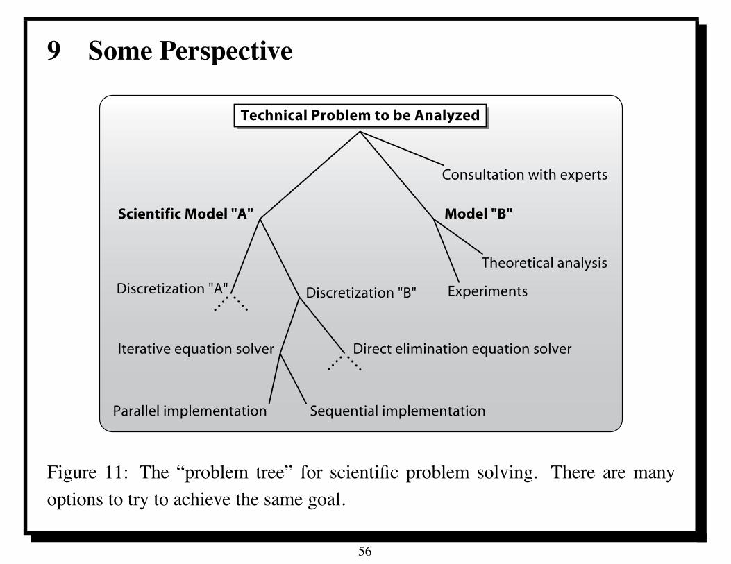
9 Some Perspective
Technical Problem to be Analyzed
Direct elimination equation solver
Discretization "A"
Scientific Model "A"
Sequential implementationParallel implementation
Iterative equation solver
Discretization "B"
Consultation with experts
Model "B"
Experiments
Theoretical analysis
Figure 11: The “problem tree” for scientific problem solving. There are manyoptions to try to achieve the same goal.
56
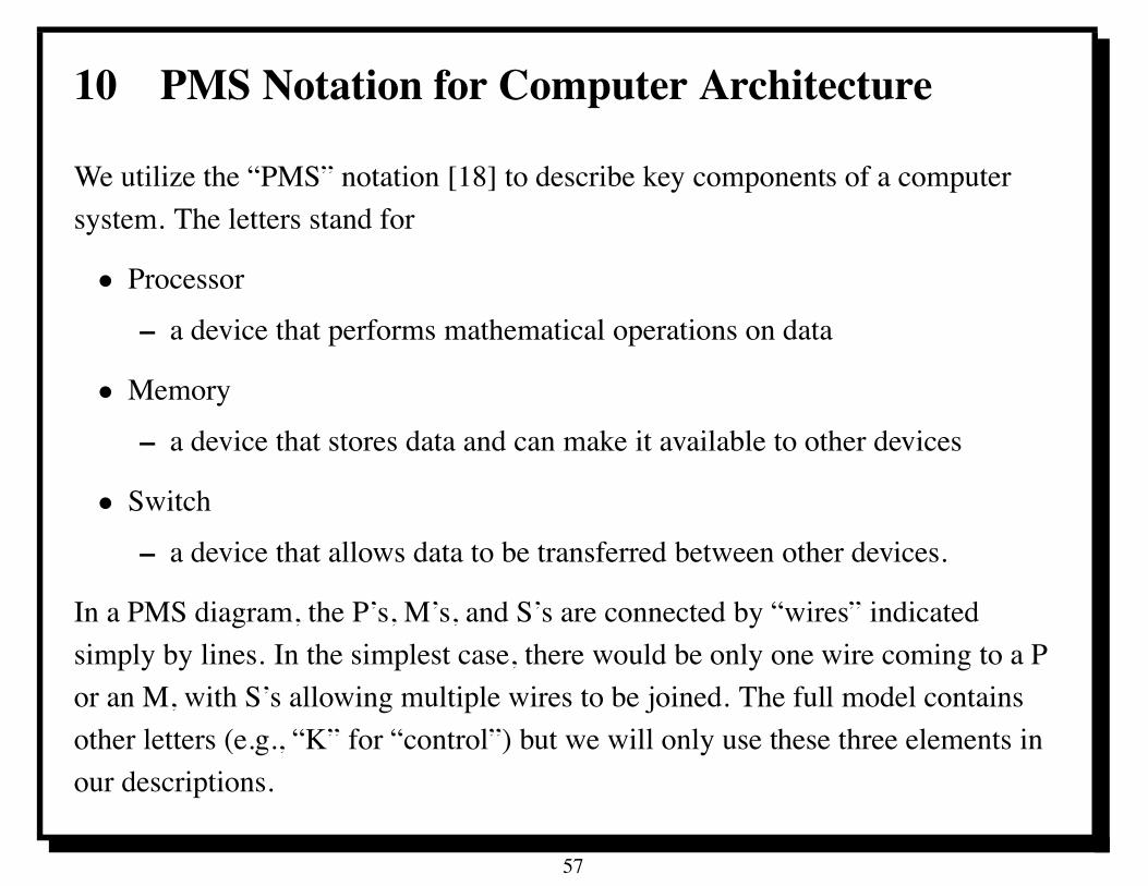
10 PMS Notation for Computer Architecture
We utilize the “PMS” notation [18] to describe key components of a computersystem. The letters stand for
• Processor
– a device that performs mathematical operations on data
• Memory
– a device that stores data and can make it available to other devices
• Switch
– a device that allows data to be transferred between other devices.
In a PMS diagram, the P’s, M’s, and S’s are connected by “wires” indicatedsimply by lines. In the simplest case, there would be only one wire coming to a Por an M, with S’s allowing multiple wires to be joined. The full model containsother letters (e.g., “K” for “control”) but we will only use these three elements inour descriptions.
57
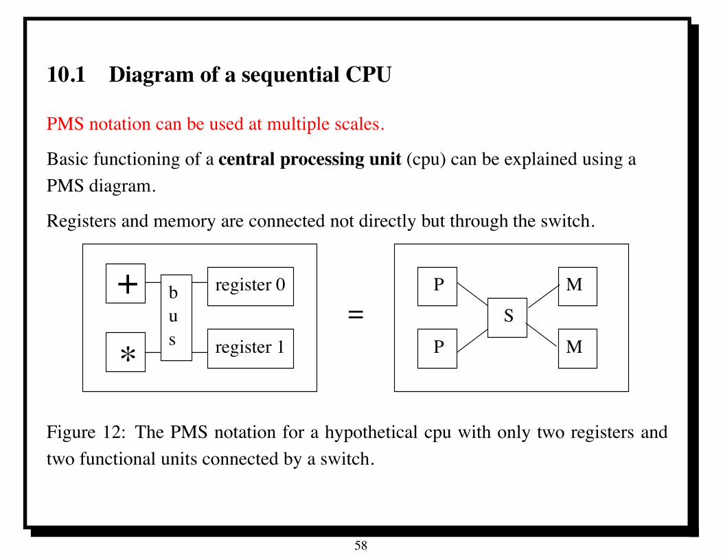
10.1 Diagram of a sequential CPU
PMS notation can be used at multiple scales.
Basic functioning of a central processing unit (cpu) can be explained using aPMS diagram.
Registers and memory are connected not directly but through the switch.
register 0
register 1*
+ bus
=P
SM
P M
Figure 12: The PMS notation for a hypothetical cpu with only two registers andtwo functional units connected by a switch.
58
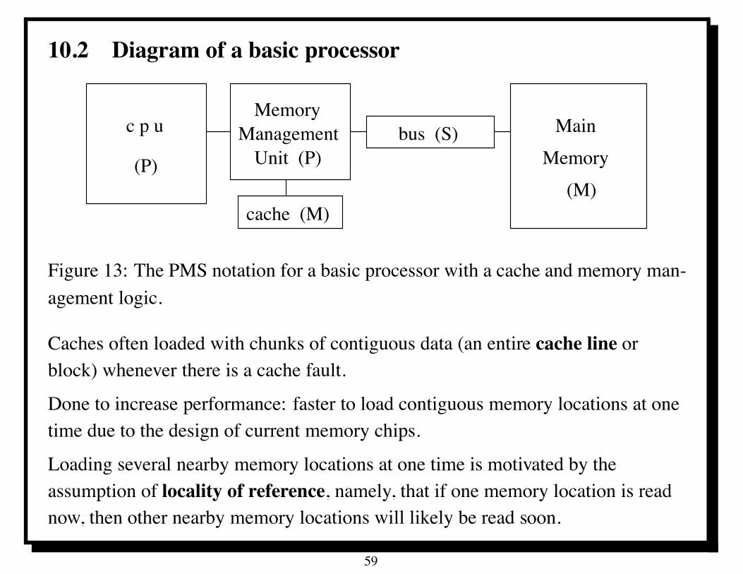
10.2 Diagram of a basic processor
MemoryManagementc p u
(P)bus (S) Main
Memory(M)
Unit (P)
cache (M)
Figure 13: The PMS notation for a basic processor with a cache and memory man-agement logic.
Caches often loaded with chunks of contiguous data (an entire cache line orblock) whenever there is a cache fault.
Done to increase performance: faster to load contiguous memory locations at onetime due to the design of current memory chips.
Loading several nearby memory locations at one time is motivated by theassumption of locality of reference, namely, that if one memory location is readnow, then other nearby memory locations will likely be read soon.
59
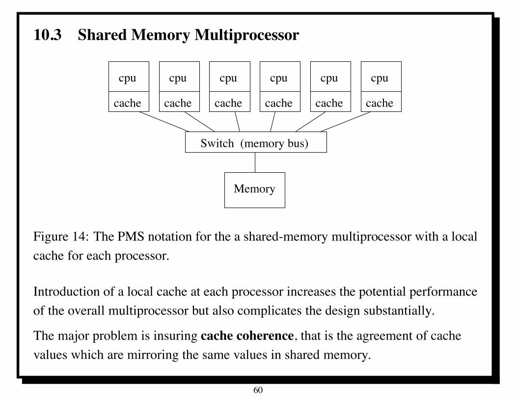
10.3 Shared Memory Multiprocessor
Memory
Switch (memory bus)
cache
cpu
cache
cpucpu cpu cpu cpu
cache cache cache cache
Figure 14: The PMS notation for the a shared-memory multiprocessor with a localcache for each processor.
Introduction of a local cache at each processor increases the potential performanceof the overall multiprocessor but also complicates the design substantially.
The major problem is insuring cache coherence, that is the agreement of cachevalues which are mirroring the same values in shared memory.
60
10.4 Shared Memory Bottleneck
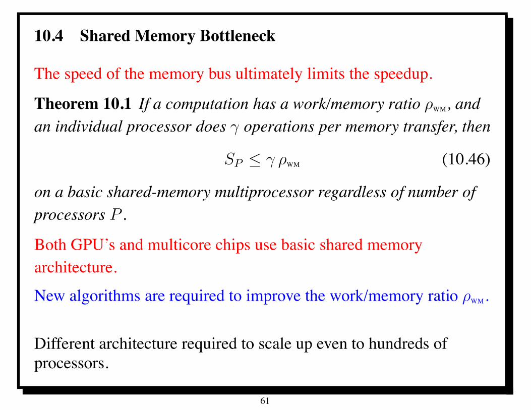
The speed of the memory bus ultimately limits the speedup.
Theorem 10.1 If a computation has a work/memory ratio !WM, andan individual processor does " operations per memory transfer, then
SP $ " !WM (10.46)
on a basic shared-memory multiprocessor regardless of number ofprocessors P .
Both GPU’s and multicore chips use basic shared memoryarchitecture.
New algorithms are required to improve the work/memory ratio !WM.
Different architecture required to scale up even to hundreds ofprocessors.
61
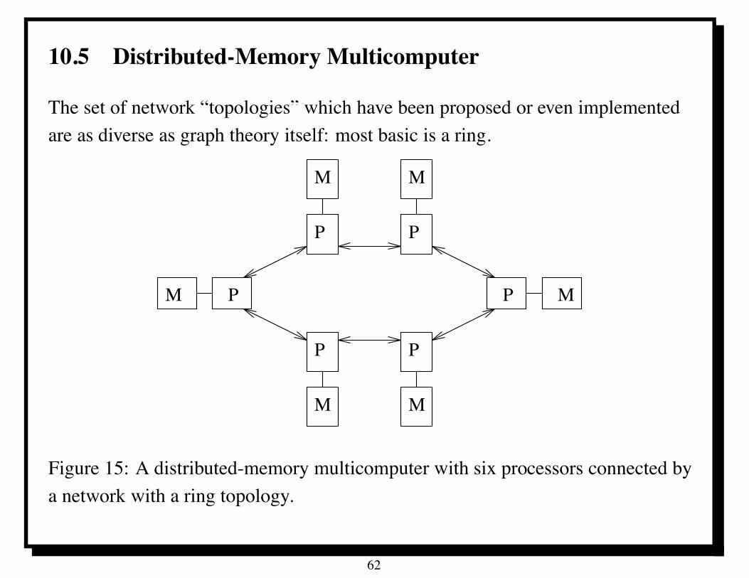
10.5 Distributed-Memory Multicomputer
The set of network “topologies” which have been proposed or even implementedare as diverse as graph theory itself: most basic is a ring.
M
P P
PP
P
M
MM
M P M
Figure 15: A distributed-memory multicomputer with six processors connected bya network with a ring topology.
62
10.6 More networks
Two and three dimensional meshes are natural extensions of rings and are used incurrent commercial parallel systems.
The two-dimensional mesh requires four connections per processor, while thethree-dimensional mesh requires six connections per processor.
Many other graphs have been proposed, and some of them have found their wayinto MPP systems.
These include trees, fat trees, and hypercubes.
Another network of current interest is based on using a cross-bar switch. Theresulting graph can be thought of as the complete graph on P nodes, i.e., all of thenodes are directly connected.
A similar type of switch effectively allows arbitrary connections through the useof amulti-stage interconnect. The connections in this case can not berepresented by a static graph. Any of the nodes can be effectively directlyconnected to any other node at any given time, but the set of simultaneousconnections cannot be very large.
63
10.7 Hypercubes
Graph: edges of a d-dimensional hypercube, vertices are at points (i1, . . . , id)
where each ij takes the value zero or one.
This can be viewed as the binary representation of an integer p in the range0 $ p $ 2d ! 1.
There are d connections per processor: bandwidth scales up as the size of theprocessor increases, but so does cost.
A related network is cube-connected cycles.
Building blocks out of a ring of d processors, each having at least three availableconnections with two used for the ring connections.
The third connection is used to connect 2d such rings in a hypercube. Thus onehas d2d processors in this approach.
Can easily be implemented with off-the-shelf technology.
64
10.8 Data exchange
The cost of exchanging data in a distributed-memory multicomputer can beapproximated by the model
&+ µ ' m (10.47)
where m is the number of words being sent, & is the “latency” corresponding tothe cost of sending a null message, i.e. a message of no length, and µ is theincremental time required to send an additional word in a message.
Model does not account for contention in the network that occurs whensimultaneous communications involve intersecting links in the network.
10.9 NOW what?
Network of workstations (NOW) is a basic (low cost) distributed-memoryparallel computer.
65
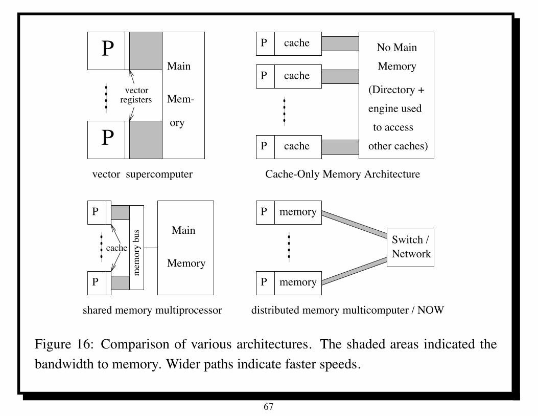
10.10 Comparison of Parallel Architectures
Figure 16 depicts quantitative and qualitative aspects of four different commercialdesigns.
The shaded areas depict the pathway from processors (including local memories,e.g. caches) to main memory.
The width of the pathway is intended to indicate relative bandwidths in thevarious designs.
It is roughly proportional to the logarithm of the bandwidth, but no attempt hasbeen made to make this exact.
The length of the pathway also indicates to some extent the latencies for thesevarious designs.
The vector supercomputer has a relatively low latency, where as thedistributed-memory computer or network of workstations has a relatively highlatency.
66
PMain
Mem-
ory
P
P
shared memory multiprocessor
P memory
P memory
P
PMemory
Main
vectorregisters
PPvector supercomputer
Memory
engine usedto access
other caches)
No Main
distributed memory multicomputer / NOW
Cache-Only Memory Architecture
cache
cache
cache
(Directory +
mem
ory
bus
cacheSwitch /Network
Figure 16: Comparison of various architectures. The shaded areas indicated thebandwidth to memory. Wider paths indicate faster speeds.
67
10.11 Contrasting Different Parallel Architectures
Figure 16 contrasts different design elements.The vector supercomputer has a relatively small local memory (its vector registers)but makes up for this in a very high bandwidth and low latency to main memory.
The COMA design provides a large local memory without sacrificing thesimplicity of shared memory.
The shared memory multiprocessor also retains this but does not have a very largelocal memory.
Finally, the distributed-memory computer or a network of workstations has a largelocal memory similar to the COMA design but cannot match the bandwidth tomain memory.
Instead of the COMA directory system, one simply has a network to transmitmessages.
Exercise: compare and contrast GPU and multicore architectures.
68
10.12 Some merits and demerits
No absolute comparisons can be made regarding the relative performance of thedifferent designs.
Different algorithms will perform differently on different architectures.
• Shared memory multiprocessor will not perform well on problems withlimited amounts of computation done per memory reference, that is, ones forwhich the work/memory ratio, "WM, is small (see Definition 4.2).
• A network of workstations cannot perform well on computations that involvea large number of small memory transfers to different processors.
• Massive bandwidth to memory made vector supercomputers relatively easy touse.
• COMA had interesting benefits but at the cost of a complex memory system(directory).
69
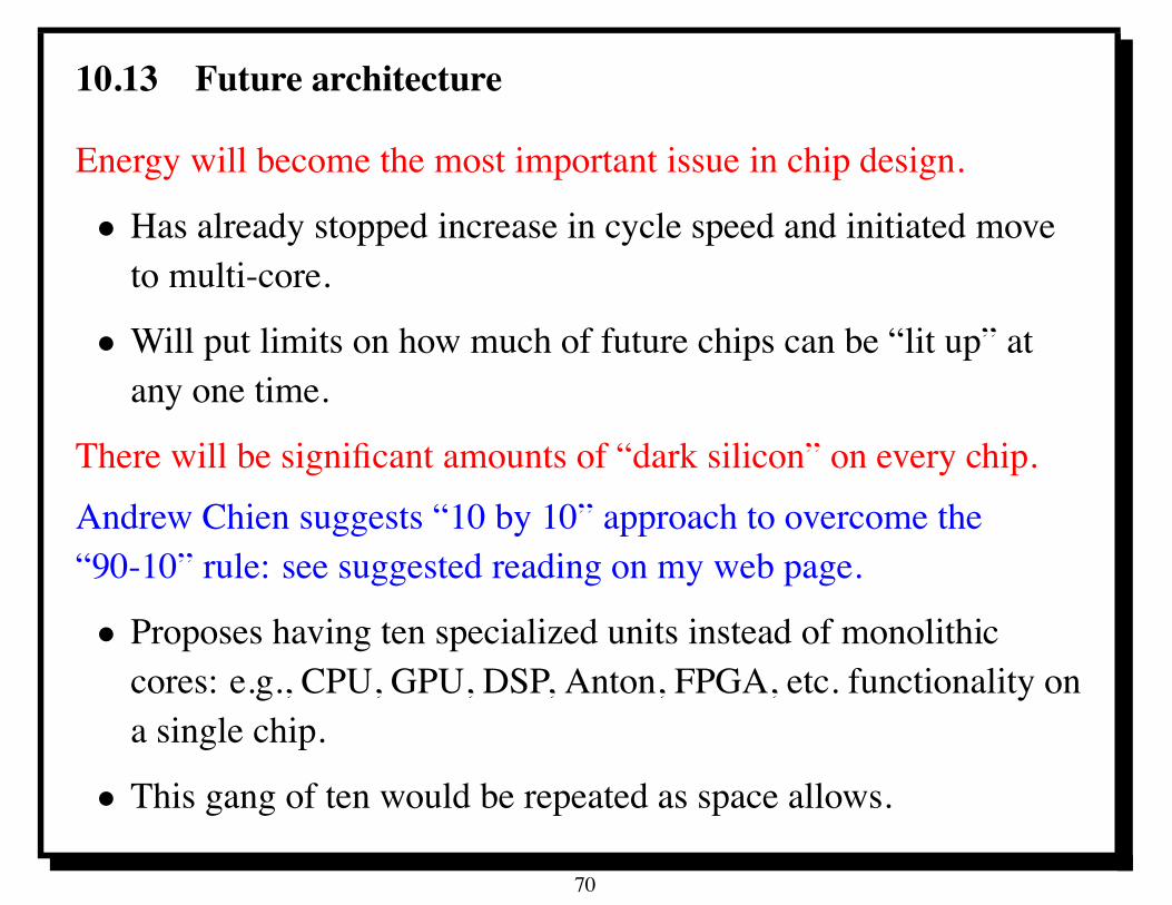
10.13 Future architecture
Energy will become the most important issue in chip design.
• Has already stopped increase in cycle speed and initiated moveto multi-core.
• Will put limits on how much of future chips can be “lit up” atany one time.
There will be significant amounts of “dark silicon” on every chip.Andrew Chien suggests “10 by 10” approach to overcome the“90-10” rule: see suggested reading on my web page.
• Proposes having ten specialized units instead of monolithiccores: e.g., CPU, GPU, DSP, Anton, FPGA, etc. functionality ona single chip.
• This gang of ten would be repeated as space allows.
70
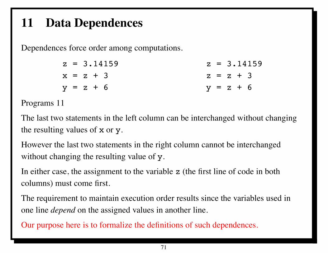
11 Data Dependences
Dependences force order among computations.
z = 3.14159 z = 3.14159x = z + 3 z = z + 3y = z + 6 y = z + 6
Programs 11
The last two statements in the left column can be interchanged without changingthe resulting values of x or y.
However the last two statements in the right column cannot be interchangedwithout changing the resulting value of y.
In either case, the assignment to the variable z (the first line of code in bothcolumns) must come first.
The requirement to maintain execution order results since the variables used inone line depend on the assigned values in another line.
Our purpose here is to formalize the definitions of such dependences.
71
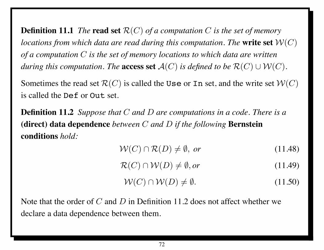
Definition 11.1 The read setR(C) of a computation C is the set of memorylocations from which data are read during this computation. The write setW(C)
of a computation C is the set of memory locations to which data are writtenduring this computation. The access set A(C) is defined to beR(C) (W(C).
Sometimes the read set R(C) is called the Use or In set, and the write set W(C)
is called the Def or Out set.
Definition 11.2 Suppose that C and D are computations in a code. There is a(direct) data dependence between C and D if the following Bernsteinconditions hold:
W(C) )R(D) *= +, or (11.48)
R(C) )W(D) *= +, or (11.49)
W(C) )W(D) *= +. (11.50)
Note that the order of C and D in Definition 11.2 does not affect whether wedeclare a data dependence between them.
72
11.1 Specific dependences and order
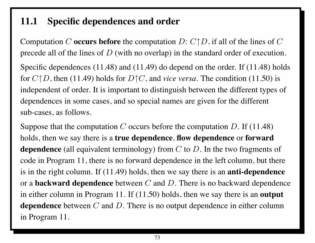
Computation C occurs before the computation D: C,D, if all of the lines of C
precede all of the lines of D (with no overlap) in the standard order of execution.
Specific dependences (11.48) and (11.49) do depend on the order. If (11.48) holdsfor C,D, then (11.49) holds for D,C, and vice versa. The condition (11.50) isindependent of order. It is important to distinguish between the different types ofdependences in some cases, and so special names are given for the differentsub-cases, as follows.
Suppose that the computation C occurs before the computation D. If (11.48)holds, then we say there is a true dependence, flow dependence or forwarddependence (all equivalent terminology) from C to D. In the two fragments ofcode in Program 11, there is no forward dependence in the left column, but thereis in the right column. If (11.49) holds, then we say there is an anti-dependenceor a backward dependence between C and D. There is no backward dependencein either column in Program 11. If (11.50) holds, then we say there is an outputdependence between C and D. There is no output dependence in either columnin Program 11.
73
11.2 Dependence implications
When there is any dependence between computations, we cannot execute them inparallel.
We are most interested in proving that there are not dependences betweencomputations in many cases.
However, proving that there are dependences between computations can halt afutile effort to parallelize code before it starts.
Dogma: if there are no dependences between two computations, they can be donein parallel.
Dependences can be different depending on different executions of the code. Forexample, the dependences in the code Program 11.2 can only be determined oncethe data i and j are read in.
read i,jx(i)=y(j)y(i)=x(j)
Program 11.2: Code with potential dependences based on I/O.
74
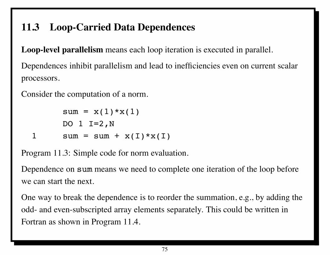
11.3 Loop-Carried Data Dependences
Loop-level parallelism means each loop iteration is executed in parallel.
Dependences inhibit parallelism and lead to inefficiencies even on current scalarprocessors.
Consider the computation of a norm.
sum = x(1)*x(1)DO 1 I=2,N
1 sum = sum + x(I)*x(I)
Program 11.3: Simple code for norm evaluation.
Dependence on sum means we need to complete one iteration of the loop beforewe can start the next.
One way to break the dependence is to reorder the summation, e.g., by adding theodd- and even-subscripted array elements separately. This could be written inFortran as shown in Program 11.4.
75
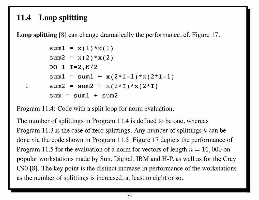
11.4 Loop splitting
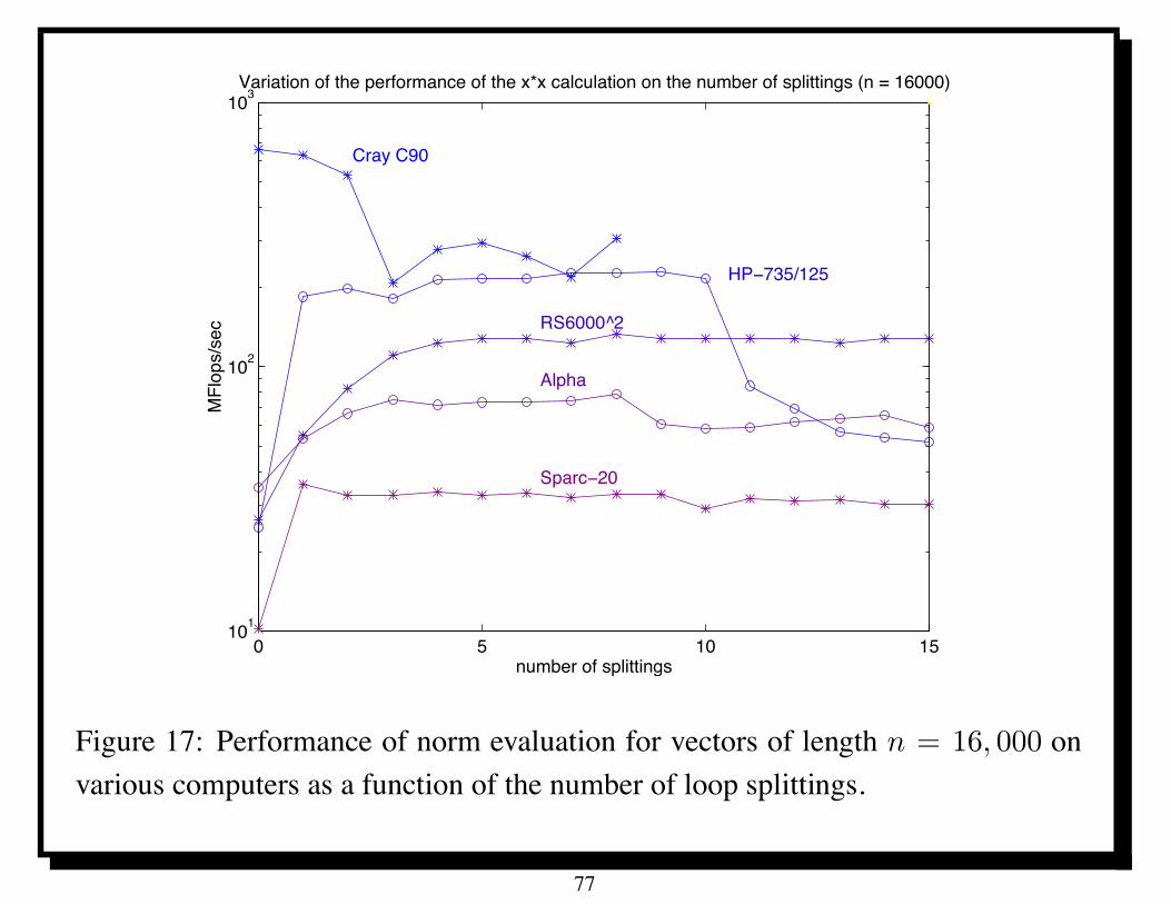
Loop splitting [8] can change dramatically the performance, cf. Figure 17.
sum1 = x(1)*x(1)sum2 = x(2)*x(2)DO 1 I=2,N/2sum1 = sum1 + x(2*I-1)*x(2*I-1)
1 sum2 = sum2 + x(2*I)*x(2*I)sum = sum1 + sum2
Program 11.4: Code with a split loop for norm evaluation.
The number of splittings in Program 11.4 is defined to be one, whereasProgram 11.3 is the case of zero splittings. Any number of splittings k can bedone via the code shown in Program 11.5. Figure 17 depicts the performance ofProgram 11.5 for the evaluation of a norm for vectors of length n = 16, 000 onpopular workstations made by Sun, Digital, IBM and H-P, as well as for the CrayC90 [8]. The key point is the distinct increase in performance of the workstationsas the number of splittings is increased, at least to eight or so.
76
0 5 10 15101
102
103
Cray C90
HP−735/125
RS6000^2
Alpha
Sparc−20
number of splittings
MFl
ops/
sec
Variation of the performance of the x*x calculation on the number of splittings (n = 16000)
Figure 17: Performance of norm evaluation for vectors of length n = 16, 000 onvarious computers as a function of the number of loop splittings.
77
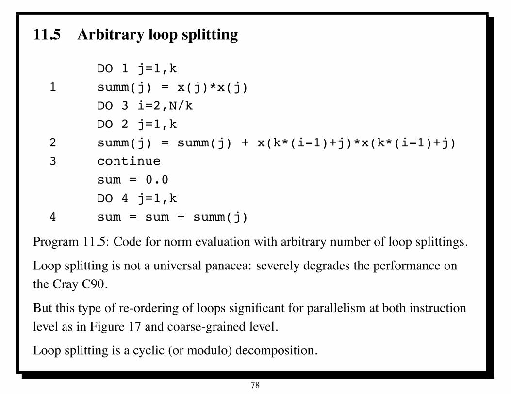
11.5 Arbitrary loop splitting
DO 1 j=1,k1 summ(j) = x(j)*x(j)
DO 3 i=2,N/kDO 2 j=1,k
2 summ(j) = summ(j) + x(k*(i-1)+j)*x(k*(i-1)+j)3 continue
sum = 0.0DO 4 j=1,k
4 sum = sum + summ(j)
Program 11.5: Code for norm evaluation with arbitrary number of loop splittings.
Loop splitting is not a universal panacea: severely degrades the performance onthe Cray C90.
But this type of re-ordering of loops significant for parallelism at both instructionlevel as in Figure 17 and coarse-grained level.
Loop splitting is a cyclic (or modulo) decomposition.
78
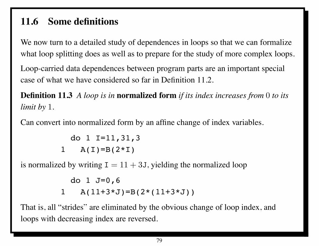
11.6 Some definitions
We now turn to a detailed study of dependences in loops so that we can formalizewhat loop splitting does as well as to prepare for the study of more complex loops.
Loop-carried data dependences between program parts are an important specialcase of what we have considered so far in Definition 11.2.
Definition 11.3 A loop is in normalized form if its index increases from 0 to itslimit by 1.
Can convert into normalized form by an affine change of index variables.
do 1 I=11,31,31 A(I)=B(2*I)
is normalized by writing I = 11 + 3J, yielding the normalized loop
do 1 J=0,61 A(11+3*J)=B(2*(11+3*J))
That is, all “strides” are eliminated by the obvious change of loop index, andloops with decreasing index are reversed.
79
The set of loop indices for normalized nested loops aremulti-indices, i.e.,n-tuples of non-negative integers, I := (i1, i2, · · · , in), where n is the number ofloops. By convention, i1 is the loop index for the outer-most loop, and so on within being the loop index for the inner-most loop. We use the symbol (0 to denote then-tuple consisting of n zeros. There is a natural total order “<” on multi-indices,lexicographical order, that is, the order used in dictionaries.
Definition 11.4 The lexicographical order for multi-indices is defined by
(i1, i2, · · · , in) < (j1, j2, · · · , jn)
whenever ik < jk for some k $ n, with i# = j# for all ) < k if k > 1.
We can then write I $ J if either I < J or I = J , and similarly we write J > J
if I < J .
The standard order of evaluation of nested (normalized) loops provides the sametotal order on the set of loop indices (i.e., on multi-indices) as the lexicographicalorder < defined in Definition 11.4. Indeed, the loop execution for index I comesbefore the loop execution for index J if and only if I < J .
80
11.7 Loop-carried dependence
If S is enclosed in at least n % 1 definite loops with main index variablesl1, l2, · · · , ln, then SI denotes the execution of S for which
(l1, l2, · · · , ln) = (i1, i2, · · · , in) =: I.
Definition 11.5 There is a loop-carried data dependence between parts S andT of a program if there are loop index vectors (i.e., multi-indices) I and J , withI < J , such that there is a data dependence between SI and TJ .
A loop-carried dependence can be described more precisely as forward (11.48),backward (11.49), or output (11.50) depending on which of the Bernsteinconditions hold.
Note that we do not assume that the parts S and T are disjoint or in any particularorder.
The ordering required following Definition 11.2 is enforced by the assumptionI < J .
In view of this, SI,TJ in Definition 11.5.
81
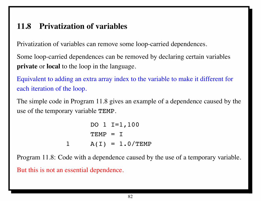
11.8 Privatization of variables
Privatization of variables can remove some loop-carried dependences.
Some loop-carried dependences can be removed by declaring certain variablesprivate or local to the loop in the language.
Equivalent to adding an extra array index to the variable to make it different foreach iteration of the loop.
The simple code in Program 11.8 gives an example of a dependence caused by theuse of the temporary variable TEMP.
DO 1 I=1,100TEMP = I
1 A(I) = 1.0/TEMP
Program 11.8: Code with a dependence caused by the use of a temporary variable.
But this is not an essential dependence.
82
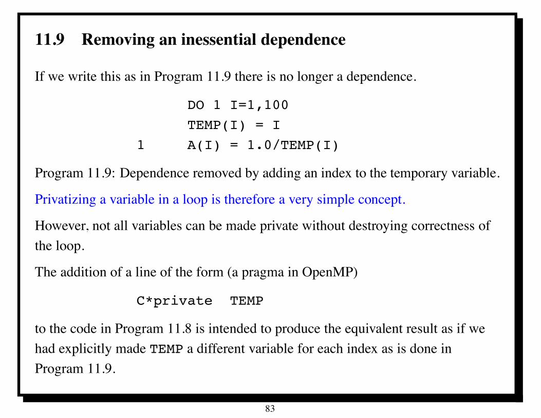
11.9 Removing an inessential dependence
If we write this as in Program 11.9 there is no longer a dependence.
DO 1 I=1,100TEMP(I) = I
1 A(I) = 1.0/TEMP(I)
Program 11.9: Dependence removed by adding an index to the temporary variable.
Privatizing a variable in a loop is therefore a very simple concept.
However, not all variables can be made private without destroying correctness ofthe loop.
The addition of a line of the form (a pragma in OpenMP)
C*private TEMP
to the code in Program 11.8 is intended to produce the equivalent result as if wehad explicitly made TEMP a different variable for each index as is done inProgram 11.9.
83
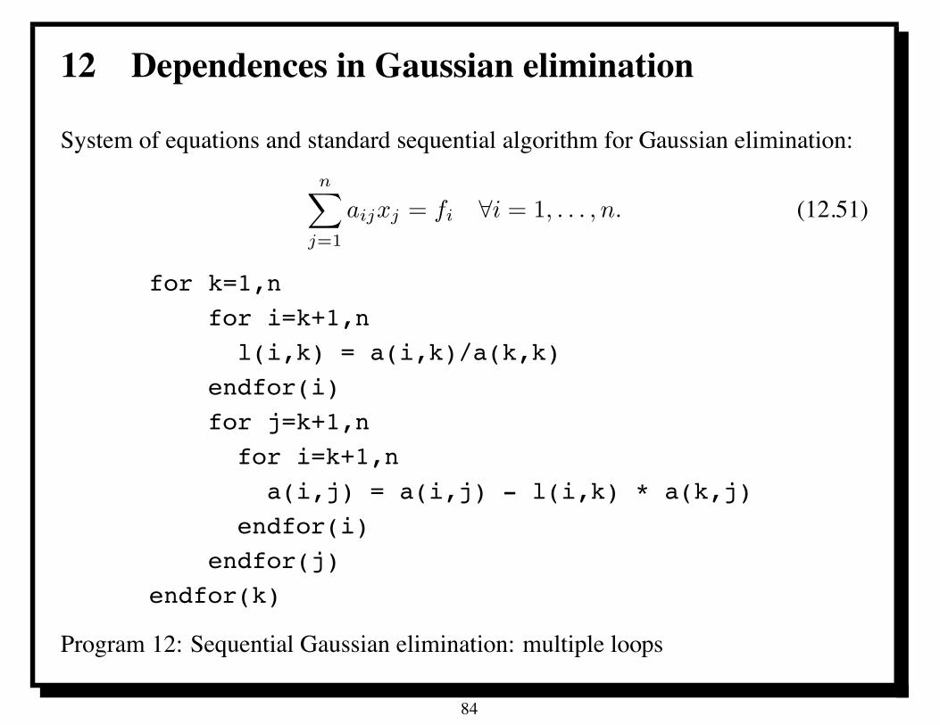
12 Dependences in Gaussian elimination
System of equations and standard sequential algorithm for Gaussian elimination:n!
j=1
aijxj = fi -i = 1, . . . , n. (12.51)
for k=1,nfor i=k+1,nl(i,k) = a(i,k)/a(k,k)
endfor(i)for j=k+1,nfor i=k+1,n
a(i,j) = a(i,j) - l(i,k) * a(k,j)endfor(i)
endfor(j)endfor(k)
Program 12: Sequential Gaussian elimination: multiple loops
84
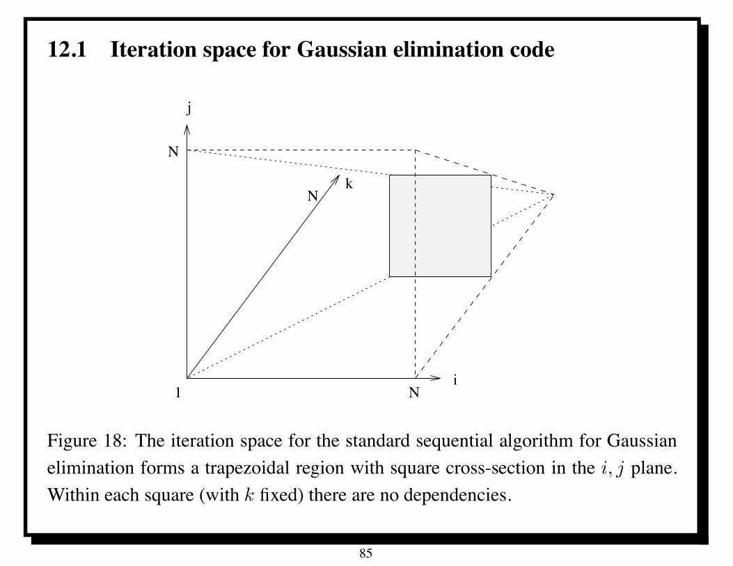
12.1 Iteration space for Gaussian elimination code
1 N
N
N
i
j
k
Figure 18: The iteration space for the standard sequential algorithm for Gaussianelimination forms a trapezoidal region with square cross-section in the i, j plane.Within each square (with k fixed) there are no dependencies.
85
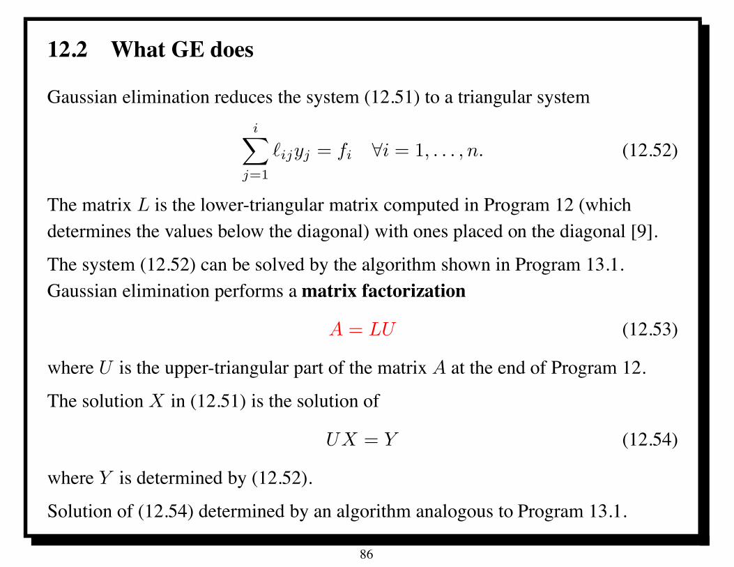
12.2 What GE does
Gaussian elimination reduces the system (12.51) to a triangular systemi!
j=1
)ijyj = fi -i = 1, . . . , n. (12.52)
The matrix L is the lower-triangular matrix computed in Program 12 (whichdetermines the values below the diagonal) with ones placed on the diagonal [9].
The system (12.52) can be solved by the algorithm shown in Program 13.1.Gaussian elimination performs amatrix factorization
A = LU (12.53)
where U is the upper-triangular part of the matrix A at the end of Program 12.
The solution X in (12.51) is the solution of
UX = Y (12.54)
where Y is determined by (12.52).
Solution of (12.54) determined by an algorithm analogous to Program 13.1.
86
12.3 Properties of GE
The dominant part of the computation in solving (12.51) is the factorizationProgram 12 in which L and U are determined.
The triangular system solves in (12.52) and (12.54) require less computation.
For this reason, we focus first on the parallelization of Program 12, returning totriangular systems in Section 13.
There are no loop-carried dependences in the inner-most two loops (the i and jloops) in Program 12 because i, j > k.
Therefore these loops can be decomposed in any desired fashion.
We now consider two different ways of parallelizing Program 12.
The algorithm in Program 12 for Gaussian elimination can be parallelized using amessage-passing paradigm as depicted in Program 12.4. It is based ondecomposing the matrix column-wise, and it corresponds to a decomposition ofthe middle loop (the j loop) in Program 12. A typical decomposition would becyclic, since it provides a good load balance.
87
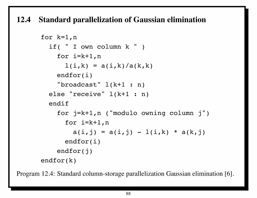
12.4 Standard parallelization of Gaussian elimination
for k=1,nif( " I own column k " )
for i=k+1,nl(i,k) = a(i,k)/a(k,k)
endfor(i)"broadcast" l(k+1 : n)
else "receive" l(k+1 : n)endif
for j=k+1,n ("modulo owning column j")for i=k+1,n
a(i,j) = a(i,j) - l(i,k) * a(k,j)endfor(i)
endfor(j)endfor(k)
Program 12.4: Standard column-storage parallelization Gaussian elimination [6].
88
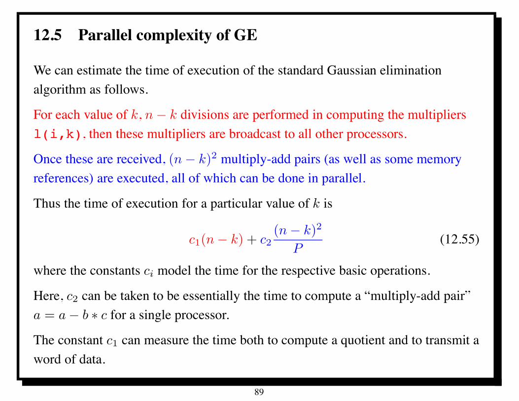
12.5 Parallel complexity of GE
We can estimate the time of execution of the standard Gaussian eliminationalgorithm as follows.
For each value of k, n ! k divisions are performed in computing the multipliersl(i,k), then these multipliers are broadcast to all other processors.
Once these are received, (n ! k)2 multiply-add pairs (as well as some memoryreferences) are executed, all of which can be done in parallel.
Thus the time of execution for a particular value of k is
c1(n ! k) + c2(n ! k)2
P(12.55)
where the constants ci model the time for the respective basic operations.
Here, c2 can be taken to be essentially the time to compute a “multiply-add pair”a = a ! b ' c for a single processor.
The constant c1 can measure the time both to compute a quotient and to transmit aword of data.
89
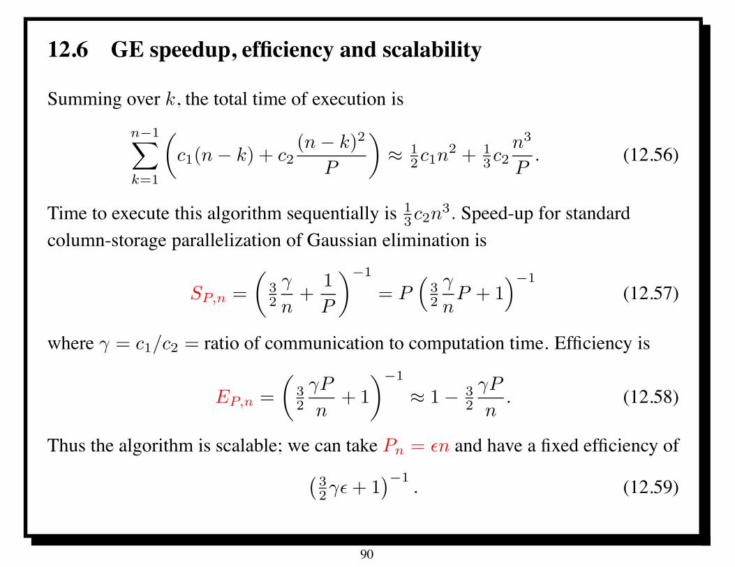
12.6 GE speedup, efficiency and scalability
Summing over k, the total time of execution isn!1!
k=1
#c1(n ! k) + c2
(n ! k)2
P
$" 1
2c1n2 + 1
3c2n3
P. (12.56)
Time to execute this algorithm sequentially is 13c2n3. Speed-up for standard
column-storage parallelization of Gaussian elimination is
SP,n =
#32
%
n+
1
P
$!1
= P&
32
%
nP + 1
'!1(12.57)
where % = c1/c2 = ratio of communication to computation time. Efficiency is
EP,n =
#32
%P
n+ 1
$!1
" 1 ! 32
%P
n. (12.58)
Thus the algorithm is scalable; we can take Pn = 'n and have a fixed efficiency of(
32%'+ 1
)!1. (12.59)
90
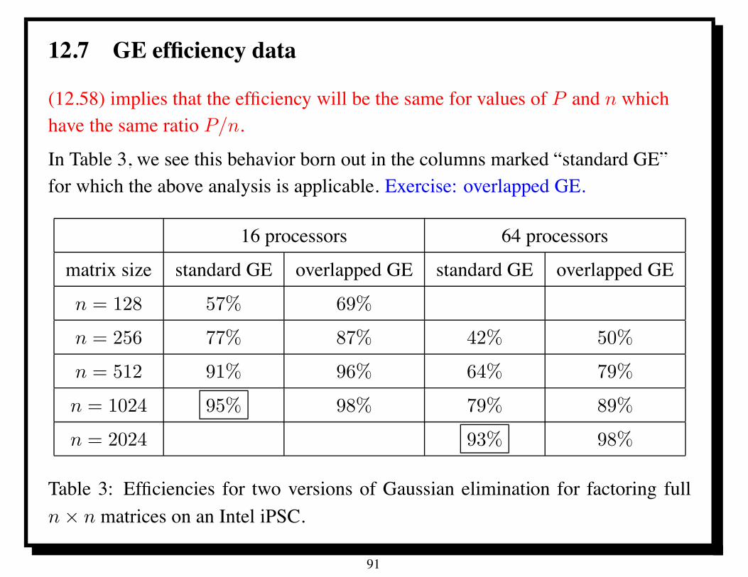
12.7 GE efficiency data
(12.58) implies that the efficiency will be the same for values of P and n whichhave the same ratio P/n.
In Table 3, we see this behavior born out in the columns marked “standard GE”for which the above analysis is applicable. Exercise: overlapped GE.
16 processors 64 processors
matrix size standard GE overlapped GE standard GE overlapped GE
n = 128 57% 69%
n = 256 77% 87% 42% 50%
n = 512 91% 96% 64% 79%
n = 1024 95% 98% 79% 89%
n = 2024 93% 98%
Table 3: Efficiencies for two versions of Gaussian elimination for factoring fulln # n matrices on an Intel iPSC.
91
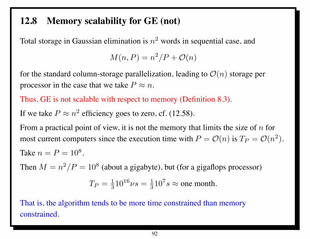
12.8 Memory scalability for GE (not)
Total storage in Gaussian elimination is n2 words in sequential case, and
M(n, P ) = n2/P + O(n)
for the standard column-storage parallelization, leading to O(n) storage perprocessor in the case that we take P " n.
Thus, GE is not scalable with respect to memory (Definition 8.3).
If we take P " n2 efficiency goes to zero, cf. (12.58).
From a practical point of view, it is not the memory that limits the size of n formost current computers since the execution time with P = O(n) is TP = O(n2).
Take n = P = 108.
Then M = n2/P = 108 (about a gigabyte), but (for a gigaflops processor)
TP = 131016*s = 1
3107s " one month.
That is, the algorithm tends to be more time constrained than memoryconstrained.
92
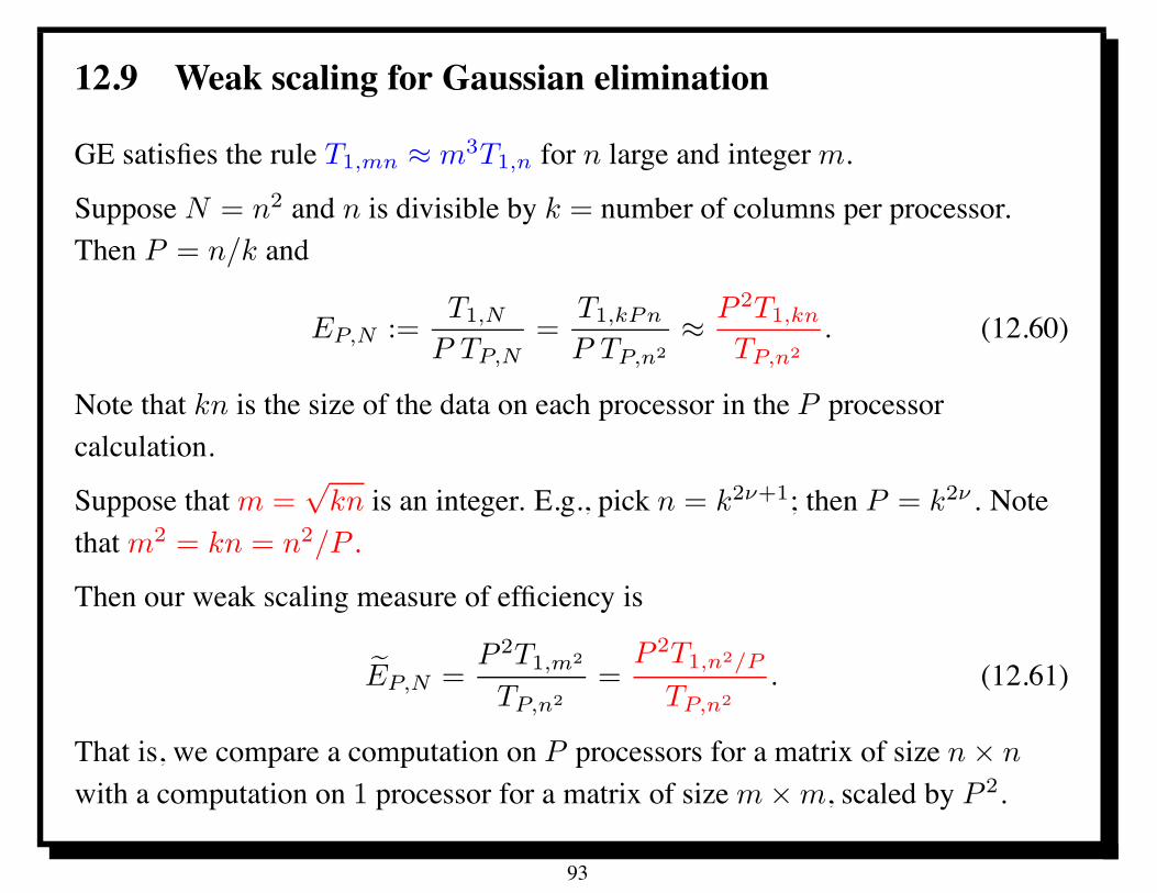
12.9 Weak scaling for Gaussian elimination
GE satisfies the rule T1,mn " m3T1,n for n large and integer m.
Suppose N = n2 and n is divisible by k = number of columns per processor.Then P = n/k and
EP,N :=T1,N
P TP,N=
T1,kPn
P TP,n2
" P 2T1,kn
TP,n2
. (12.60)
Note that kn is the size of the data on each processor in the P processorcalculation.
Suppose that m =&
kn is an integer. E.g., pick n = k2$+1; then P = k2$ . Notethat m2 = kn = n2/P .
Then our weak scaling measure of efficiency is
*EP,N =P 2T1,m2
TP,n2
=P 2T1,n2/P
TP,n2
. (12.61)
That is, we compare a computation on P processors for a matrix of size n # n
with a computation on 1 processor for a matrix of size m # m, scaled by P 2.
93
13 Solving triangular systems in parallel
Key to the scalability of Gaussian elimination (GE) is the fact that thework/memory ratio "WM = n.
However, triangular solution has a work/memory ratio "WM = 1.
Gaussian elimination reduces a square system of equations to a traingular one (seeSection 12).
The latter is (sequentially) trivial to solve, if one starts at the correct end of thetriangle [9].
An algorithm for a lower triangular system (with matrix a like the matrix lgenerated in Program 12) is in Program 13.1.
There are now loop-carried dependences in both the i and k loops (exercise),although the inner loop is a reduction.
These loops cannot easily be parallelized, but we will see in Section 13.3 that theycan be decomposed in a suggestive way (see Figure 19).
94
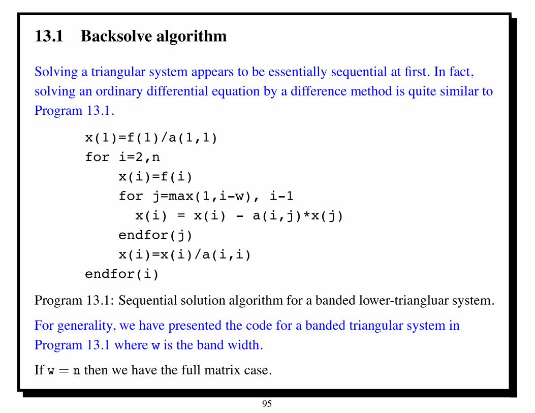
13.1 Backsolve algorithm
Solving a triangular system appears to be essentially sequential at first. In fact,solving an ordinary differential equation by a difference method is quite similar toProgram 13.1.
x(1)=f(1)/a(1,1)for i=2,n
x(i)=f(i)for j=max(1,i-w), i-1x(i) = x(i) - a(i,j)*x(j)
endfor(j)x(i)=x(i)/a(i,i)
endfor(i)
Program 13.1: Sequential solution algorithm for a banded lower-triangluar system.
For generality, we have presented the code for a banded triangular system inProgram 13.1 where w is the band width.
If w = n then we have the full matrix case.
95
13.2 Triangular scenarios
Solving a triangular system just once: Typically occurs when the triangular systemarises via matrix factorization. Since the time for a single triangular system solveis minor compared with matrix factorization, the cost of the triangular system isnegligible. Even modest efforts at parallelization may be useful.
Solving a triangular system with many right-hand sides, all available at one time:Due to the large amount of data (the right-hand sides), there are specialopportunities for parallelism which make triangular solution appear similar incharacter to the factorization problem.
Solving a triangular system with many right-hand sides, only one of which isavailable at a time: This occurs when solving time-dependent problems ornon-linear problems in which the triangular system is part of an inner loop. Theright-hand side changes as the outer loop progresses. In this case, any initialpre-processing of the triangular system can be amortized. The issue is justproducing a solution as quickly as possible.
This is most challenging situation to parallelize efficiently, and therefore we willconcentrate on this case.
96
13.3 The “toy duck” algorithm
Let us begin by considering a straight-forward parallelization of the standardalgorithm shown in Program 13.1; similar to overlapped GE.
We will compute the same arithmetic operations in the same order, but we willorganize them in a way that presents independent tasks that can be done inparallel.
We describe the )-th stage for ) > 1 assuming all needed information has beeninitialized; Figure 19 depicts the various computations done at this stage.
Initialization phase left as an exercise.
We assume that k is a parallelization parameter that will be specified later.
It will be a positive integer less than 12w.
At the )-th step, we assume that all xi’s for i $ k) have already been computedand distributed to each processor.
At each step, solution values xi will be computed for k new indices i anddistributed to each processor.
97
0k
12
P-1
w
maindiagonal
k
k
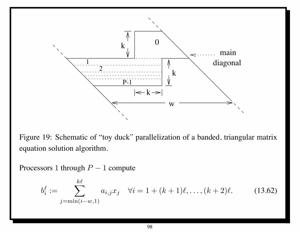
Figure 19: Schematic of “toy duck” parallelization of a banded, triangular matrixequation solution algorithm.
Processors 1 through P ! 1 compute
b#i :=
k#!
j=min(i!w,1)
ai,jxj -i = 1 + (k + 1)), . . . , (k + 2)). (13.62)
98
13.4 Typical step in toy duck
In the simplest case (as we now assume) we will have
k = *(P ! 1) (13.63)
for some integer * % 1, so that each processor % 1 computes * different bi’susing previously computed xj’s.
Note that this requires access to the (previously computed) values xj for j $ k).
Simulaneously, processor 0 computes xk#+1, . . . , x(k+1)# by the standardalgorithm, namely,
xi = a!1i,i
+
,fi ! b#!1i !
i!1!
j=(k!1)#+1
ai,jxj
-
. -k) < i $ (k + 1)). (13.64)
We can assume that a!1i,i has been precomputed and stored, if desired.
At end of this step, processor 0 sends xk#+1, . . . , x(k+1)# to other processors, andother processors send b(k+1)#+1, . . . b(k+2)# to processor 0.
99
13.5 Analysis of toy duck
This completes the )-th step for ) > 1.
These steps involve a total of 2k2 MAPS, where MAPS stands formultiply-addpairs.
Load balance in (13.62) can be achieved in a number of ways.
If * = 2, then perfect load balance is achieved by having processor 1 doing thefirst and last row, processor 2 doing the second and penultimate row, and so on.
The total number of operation to compute (13.62) is
k(w ! k) ! 12k2 = kw ! 3
2k2 (13.65)
MAPS, where MAPS stands for “multiply-add pairs.”
Thus the time estimate for (13.62) is proportional to(w ! 3
2k) k
P ! 1(13.66)
time units, where the unit is taken to be the time required to do one multiply-addpair.
100
13.6 Continued analysis of toy duck
Processor zero does 32k2 MAPS, and thus the total time for one stage of the
program is proportional to
max/
32k2,
(w ! 3
2k) k
P ! 1
0. (13.67)
These are balanced if32k2 =
(w ! 3
2k) k
P ! 1(13.68)
which reduces to havingP = 2
3
w
k. (13.69)
Recalling our assumption (13.63), we find that
P (P ! 1) = 23
w
*(13.70)
Optimal P depends only on the band width w and not on n. Algorithm notscalable in usual sense (Definition 8.2) if w remains fixed independently of n.
101
13.7 Scaling of toy duck
Total amount of data communicated at each stage is 2k words.
(13.68) implies that computational load is proportional to k2, so this algorithm isscalable if w . / as n . / (exercise).
The case of a full matrix corresponds to w = n.
The “toy duck” algorithm has substantial parallelism in this case.
For fixed *, (13.70) implies that P is proportional to&
w, and this in turn impliesthat k is proportional to
&w.
The amount of memory per processor is directly proportional to the amount ofwork per processor, so this is proportional to k2, and hence w, in the balancedcase (13.68).
102

13.8 A block inverse algorithm
The following algorithm can be found in [15]. Let us write the lower triangularmatrix L as a block matrix. Suppose that n = ks for some integers k and s.
+
11111111111,
L1 0 0 0 0 0
R1 L2 0 0 0 0
0 R2 L3 0 0 0
0 0 · · · · · · 0 0
0 0 0 Rk!2 Lk!1 0
0 0 0 0 Rk!1 Lk
-
22222222222.
(13.71)
A triangular matrix is invertible if and only if its diagonal entries are not zero (see[9] or just apply the solution algorithm in Program 13.1). Thus any sub-blocks onthe diagonal will be invertible as well if L is, as we now assume. That is, each Li
is invertible, no matter what choice of k we make.
103
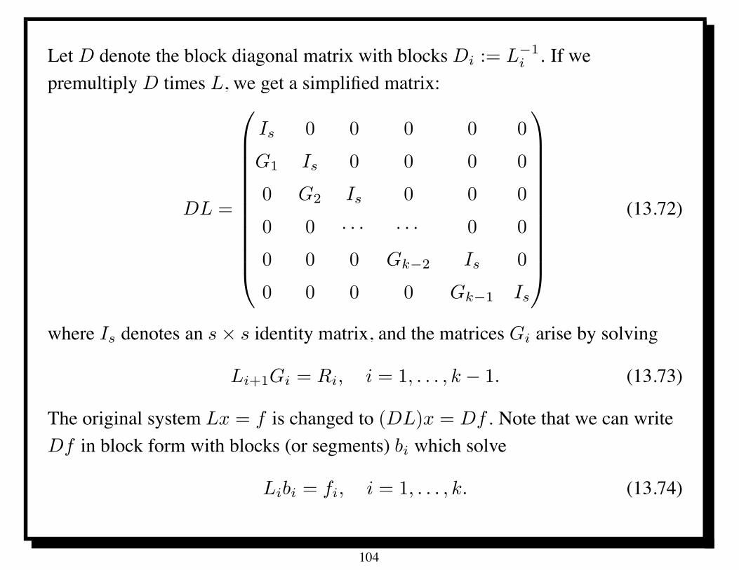
Let D denote the block diagonal matrix with blocks Di := L!1i . If we
premultiply D times L, we get a simplified matrix:
DL =
+
11111111111,
Is 0 0 0 0 0
G1 Is 0 0 0 0
0 G2 Is 0 0 0
0 0 · · · · · · 0 0
0 0 0 Gk!2 Is 0
0 0 0 0 Gk!1 Is
-
22222222222.
(13.72)
where Is denotes an s # s identity matrix, and the matrices Gi arise by solving
Li+1Gi = Ri, i = 1, . . . , k ! 1. (13.73)
The original system Lx = f is changed to (DL)x = Df . Note that we can writeDf in block form with blocks (or segments) bi which solve
Libi = fi, i = 1, . . . , k. (13.74)
104
13.9 Block inverse details
The blocks Li in (13.74) are s # s lower-triangular matrices with bandwidth w, sothe band algorithm Program 13.1 is appropriate to solve (13.74).
Depending on the relationship between the block size s and the band width w,there may be a certain number of the first columns of the matrices Ri which areidentically zero.
In particular, one can see (exercize) that the first s ! w columns are zero.
Due to the definition of Gi, the same must be true for them as well (exercize).
Let %Gi denote the right-most w columns of Gi = (0 %Gi)
let Mi denote the top s ! w rows of %Gi and
let Hi denote the bottom w rows of %Gi.
Further, split bi similarly, with
ui denoting the top s ! w entries of bi and
vi denoting the bottom w entries of bi.
105
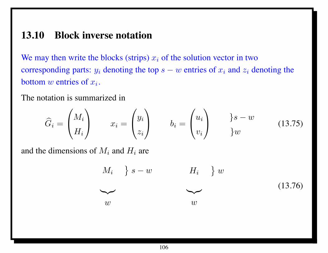
13.10 Block inverse notation
We may then write the blocks (strips) xi of the solution vector in twocorresponding parts: yi denoting the top s ! w entries of xi and zi denoting thebottom w entries of xi.
The notation is summarized in
%Gi =
+
,Mi
Hi
-
. xi =
+
,yi
zi
-
. bi =
+
,ui
vi
-
. }s ! w
}w(13.75)
and the dimensions of Mi and Hi are
Mi
3s ! w
4567w
Hi
3w
4567w
(13.76)
106
13.11 Block inverse reduction
All of these quantities have now simple relationships. First of all we have
y1 = u1, z1 = v1 (13.77)
we can inductively determine the zi’s by
zi+1 = vi+1 ! Hizi -i = 1, . . . , k ! 1 (13.78)
Then we can separately determine the yi’s by
yi+1 = ui+1 ! Mizi -i = 1, . . . , k ! 1 (13.79)
There are no dependences in (13.79), but (13.78) appears at first to be sequential.
However, if w is sufficiently large, there is an opportunity for parallelism in eachiteration of (13.78).
Moreover, (13.78) can be written as a lower-triangular system itself, and wedescribe an appropriate parallel solution algorithm.
107
There are two cases to distinguish in applying the above algorithm. One is thecase where a system is solved only once, and the systems (13.73) become a majorpart of the computation. The other is the case where a system is solved manytimes, and the cost of solving the systems (13.73) can be amortized since theyneed be solved only once.
The primary amount of work in (13.74) is
k(ws ! 1
2w2)
= wn ! 12
w2n
s(13.80)
MAPS, whereas the primary amount of work in (13.78) is
w2(k ! 1) =w2(n ! s)
s(13.81)
MAPS, and the primary amount of work in (13.79) is
w(s ! w)(k ! 1) =w(s ! w)(n ! s)
s= wn ! w2n
s! w(s ! w) (13.82)
MAPS.
108
13.12 Block inverse analysis
The sum of (13.80), (13.81) and (13.82) is nearly 2nw, twice the amount of workin the sequential case (Program 13.1).
The amount of parallelism in (13.78) is complex to assess [16], but once all thezi’s are computed (and appropriately distributed), (13.79) can be done (trivially)in parallel.
Moreover, (13.80) can also be computed trivially in parallel.
If (13.78) is computed sequentially, then
TP % wn
#w
s+
1
P
&1 ! w
s
'$= wn
#wP
n+
1
P
#1 ! wP
n
$$(13.83)
if P = k. Therefore
E!1P % wP 2
n+
#1 ! wP
n
$(13.84)
Taking P $8
n/w would be required for a scalable algorithm.
109
14 Parallel prefix
Assume the lower triangular matrix L is already of the form
xi + Hi!1xi!1 = vi -i = 1, . . . , 2% (14.85)
where all undefined quantities (H0, H1, x0, etc.) are set implicitly to zero.
Then the relation (14.85) between subsequent blocks of the solution x can bewritten in an extended (specifically, (w + 1) # (w + 1)) block matrix form as
+
,xi
1
-
. =
+
,!Hi!1 vi
0w 1
-
.
+
,xi!1
1
-
. =: hi
+
,xi!1
1
-
. (14.86)
where 0w denotes a row vector of zeros of length w and hi denotes the indicated(w + 1) # (w + 1) matrix.
Parallel prefix applies to any associative operation 0 and produces
gi := hi 0 hi!1 0 · · ·0 h1, i = 1, . . . , 2%
using a binary tree [12].
110
14.1 Parallel prefix application
Applying induction, we thus see that+
,xi
1
-
. = gi
+
,0w
1
-
. (14.87)
where gi := hi 0 hi!1 0 · · ·0 h1 and 0 is matrix multiplication for(w + 1) # (w + 1) matrices.
Therefore, we may use parallel prefix to compute the (w + 1) # (w + 1) matricesgi and then recover the solution from (14.87).
Parallel prefix requires 2+ steps involving matrix multiplication of two(w + 1) # (w + 1) matrices, and communication (along edges of a tree) whichsend a (w + 1) # (w + 1) matrix at each step.
The computation is O(+w3) and the communication is O(+w2).
111
14.2 Parallel prefix not good alone
In the special case that s = w in the algorithm in Section 13.8, the matrices Mi
disappear and Gi = Hi.
We can thus think of (14.85) as a special case of (13.71).
Parallel prefix applied to this problem requires O(+w3) time compared with nw
time in the sequential case.
A speedup of n/+w2 is the largest possible with parallel prefix alone. Theefficiency would satisfy (recall that n = Pw)
E!1P =
P+w3
nw=
P+w2
n= +w = w log2 P (14.88)
which does not imply scalability.
Thus parallel prefix alone is not a scalable triangular solver.
However, we now look at combining it with other algorithms.
112
14.3 Combining with parallel prefix
If (13.78) is computed by parallel prefix then time estimate in (13.83) becomes
TP " wn
#w2
nlog2 P +
1
P
#2 ! 3wP
2n+
w
n! 1
P
$+ %
w
nlog P
$, (14.89)
where % = ratio of communication to computation time in parallel prefix. Thus
E!1P "
#w2
n+%w
n
$P log2 P +
#2 ! 3wP
2n+
w
n! 1
P
$
=w2 + %w
slog2 P +
#2 ! 3w
2s+
w
n! 1
P
$.
(14.90)
We assume k = P = 2%.
Theorem 14.1 The algorithm in Section 13.8, where (13.78) is solved by parallelprefix, is scalable for P log2 P $ cn/(w2 + %w) for any fixed c < /. Inparticular, we must take s % max{w, '(w2 + %w) log2 P} for some ' > 0.
The expression w2 + %w in the theorem can be improved to w2 + $w + & where& is the latency and $ measures bandwidth.
113
15 Scalable solution of non-linear time-dependentsystems
Mark Maienschein-Cline
Department of Chemistry
University of Chicago
and
L. Ridgway Scott
114
15.1 Initial value problems
Finite difference methods for solving initial value problem for an ordinarydifferential equation exhibit limited natural parallelism.
However, for linear systems there are scalable parallel algorithms in which thedomain decomposition is in the time domain.
Such techniques are based on scalable methods for solving banded triangularlinear systems of equations and have been known for some time (cf. [15, 12]).
What can provide the increasing data size needed for such scalability is a longtime interval of integration.
Indeed, there are many simulations in which the primary interest is a very longtime of integration.
For example, there is a celebrated simulation of the villin headpiece by moleculardynamics [5].
115
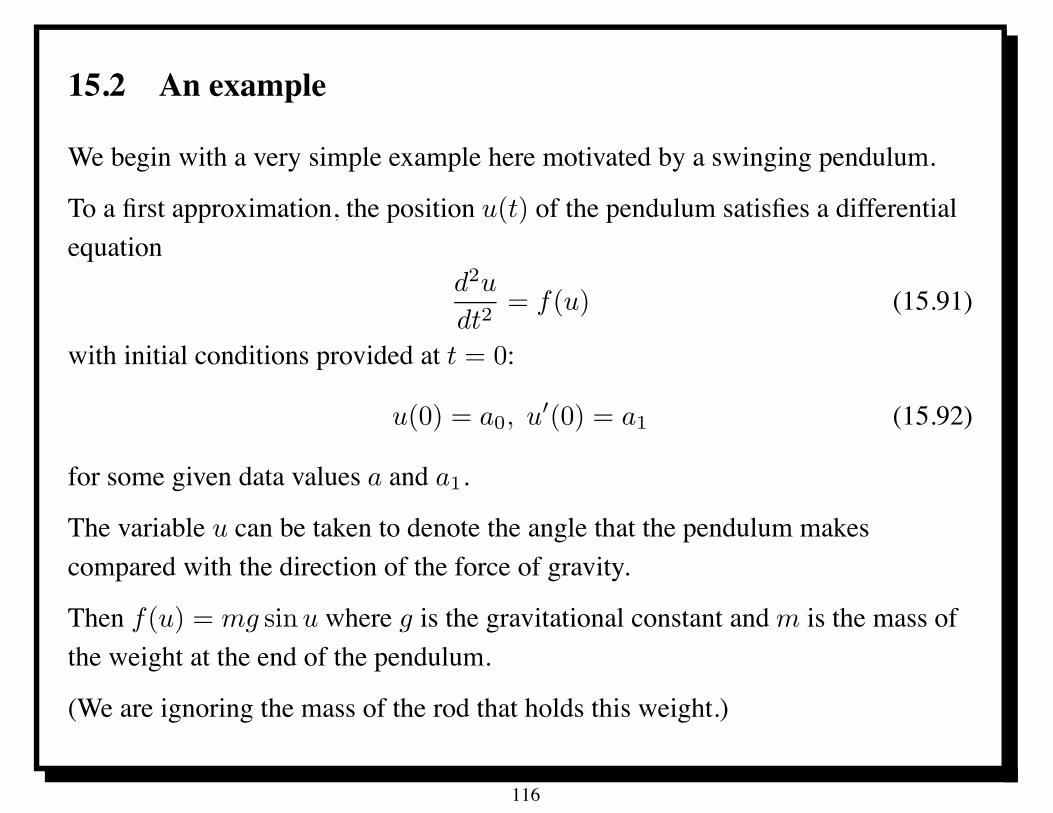
15.2 An example
We begin with a very simple example here motivated by a swinging pendulum.
To a first approximation, the position u(t) of the pendulum satisfies a differentialequation
d2u
dt2= f(u) (15.91)
with initial conditions provided at t = 0:
u(0) = a0, u#(0) = a1 (15.92)
for some given data values a and a1.
The variable u can be taken to denote the angle that the pendulum makescompared with the direction of the force of gravity.
Then f(u) = mg sin u where g is the gravitational constant and m is the mass ofthe weight at the end of the pendulum.
(We are ignoring the mass of the rod that holds this weight.)
116
15.3 Dicretization
We can approximate via a central difference method to get a recursion relation
un+1 = 2un ! un!1 ! ,f(un) (15.93)
where , := !t2.
If the displacements of the pendulum position from vertical are small, then we canuse the approximation sinu " u to get a linear equation
d2u
dt2= mgu. (15.94)
In this case, the difference equations become a linear recursion relation of the form
un+1 = (2 ! ,mg) un ! un!1. (15.95)
The initial conditions (15.92) provide starting values for the the recursion. Forexample, we can take
u0 = a and u!1 = a0 ! a1!t. (15.96)
This allows us to solve (15.95) for n % 0.
117
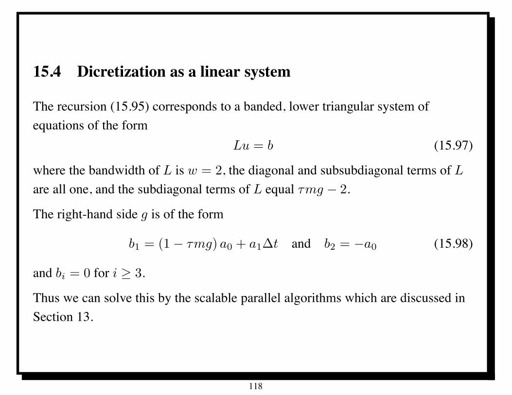
15.4 Dicretization as a linear system
The recursion (15.95) corresponds to a banded, lower triangular system ofequations of the form
Lu = b (15.97)
where the bandwidth of L is w = 2, the diagonal and subsubdiagonal terms of L
are all one, and the subdiagonal terms of L equal ,mg ! 2.
The right-hand side g is of the form
b1 = (1 ! ,mg) a0 + a1!t and b2 = !a0 (15.98)
and bi = 0 for i % 3.
Thus we can solve this by the scalable parallel algorithms which are discussed inSection 13.
118
15.5 Nonlinear systems
When f is not linear, such algorithms are not directly applicable.
We can formulate a set of equations to define the entire vector of values ui as anensemble, but it is no longer a linear equation.
We can write it formally asF (U) = 0 (15.99)
where F is defined by
F (U) = L0U + ,mg-(U) ! b (15.100)
with L0 the same as L above with , = 0, that is L0 is a lower triangular matrixwith bandwidth w = 2, the diagonal and subsubdiagonal terms of L0 are all one,and the subdiagonal terms of L0 equal !2. The function - thus contains all of thenonlinearity and has the simple form
-(U)ij = .j,i!1 sinui!1 (15.101)
where .i,j is the Kronecker delta.
119
15.6 Newton’s method
The Newton-Raphson method can be written in the form
F #(Un)(Un+1 ! Un
)= !F (Un). (15.102)
where F # is the Jacobian matrix of all partial derivatives of F with respect to thevector U .
To see how this works, let us return to the pendulum problem. In the case of thependulum, we have F defined by (15.100). It takes a careful look at the definition,but it is not hard to see that the Jacobian matrix for a linear function of the formU . L0U is the matrix L0. Thus JF (U) = L0 + ,mgJ&(U). With - of the form(15.101), it can be shown that
J&(U)ij = .j,i!1-#(ui!1) = .j,i!1 cosui!1. (15.103)
The Jacobian has the same form as the original matrix L. In fact, if F is linear,Newton’s method is equivalent to just solving the system (15.97) and converges inone step.
120
15.7 Linearized initial value problem
There is another way to interpret the Newton algorithm for solving the initialvalue problem.
Suppose that we have an approximate solution u to (15.91) which satisfies theinitial conditions (15.92), and define the residual R(u) by
R(u) :=d2u
dt2! f(u) (15.104)
which is a function of t defined on whatever interval u is defined on.
We can apply Newton’s method (in the appropriate infinite dimensional setting) tosolve
R(u) = 0. (15.105)
Let us derive the resulting equations by an elementary approach.
121
15.8 Newton step derivation
Suppose that we try to add a perturbation v to u to get it to satisfy (15.91) (more)exactly. We use a Taylor expansion to write
f(u + v) = f(u) + vf #(u) + O(v2) (15.106)
Thus the sum u + v satisfies an initial value problem of the form
d2(u + v)
dt2! f(u + v) =
d2v
dt2! vf #(u) + R(u) + O(v2). (15.107)
With (15.107) as motivation, we now define v by solving the initial value problem
d2v
dt2= vf #(u) ! R(u) (15.108)
with initial conditions provided at t = 0:
v(0) = 0, v#(0) = 0. (15.109)
Then the Newton step for solving (15.105) is the solution v of (15.108-15.109).
122
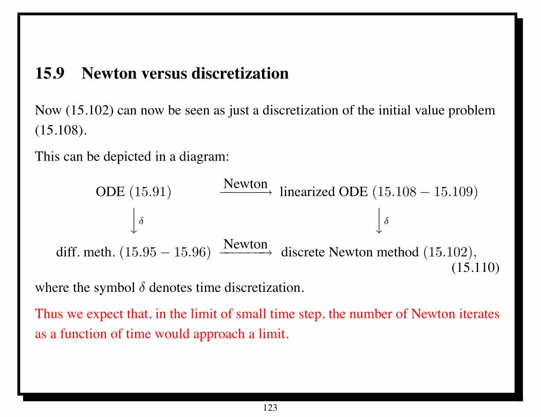
15.9 Newton versus discretization
Now (15.102) can now be seen as just a discretization of the initial value problem(15.108).
This can be depicted in a diagram:
ODE (15.91)Newton!!!!!!. linearized ODE (15.108 ! 15.109)
99:'
99:'
diff. meth. (15.95 ! 15.96)Newton!!!!!!. discrete Newton method (15.102),
(15.110)where the symbol . denotes time discretization.
Thus we expect that, in the limit of small time step, the number of Newton iteratesas a function of time would approach a limit.
123
15.10 Getting Newton started
Newton’s method (15.102) converges rapidly once you get close to a solution, buthow do you get close in the first place? This does not have a good answer ingeneral, but we can indicate one type of approach here. Suppose that we had asimplified approximation f to f and we solved
d2u
dt2= f(u) (15.111)
exactly, together with the initial conditions (15.92). For example, withf(u) = sinu we might have f(u) = u as an approximation. This makes (15.111)linear, and in this simple case we can even solve the equation in closed form (interms of sines and cosines). It is much faster to evaluate f(u) in this case than it isf(u), so the computation of the initial guess would be much less costly.
124
If we use the solution u to (15.111) as the starting guess for Newton’s method,then the initial residual R(u) has a simple interpretation. We can express it simplyas
R(u) =d2u
dt2! f(u) = f(u) ! f(u). (15.112)
Thus the size of the residual is simply related to the error in approximation of f
by f . Since the first Newton step v satisfies (15.108), we can bound the size of v
in terms of R(u), and hence f ! f . More precisely, (15.108) becomes
d2v
dt2= vf #(u) !
&f(u) ! f(u)
'. (15.113)
Since v is zero at the start (see (15.92)), it will be small for at least somereasonable interval of time. The size of v can be predicted as u is computed, andthe process can be stopped if the prediction gets too large. Thus there is a naturalway to control the size of the Newton step in this case.
125
It would be possible to approximate on a coarser mesh as well. That is, we coulduse a larger !t in (15.93) (recall that , = !t2). It would then be necessary tointerpolate onto a finer mesh to define the residual appropriate for (15.108) (orequivalently in (15.102) in the discretized case). In this way, a multi-gridapproach could be developed in the time variable.
126
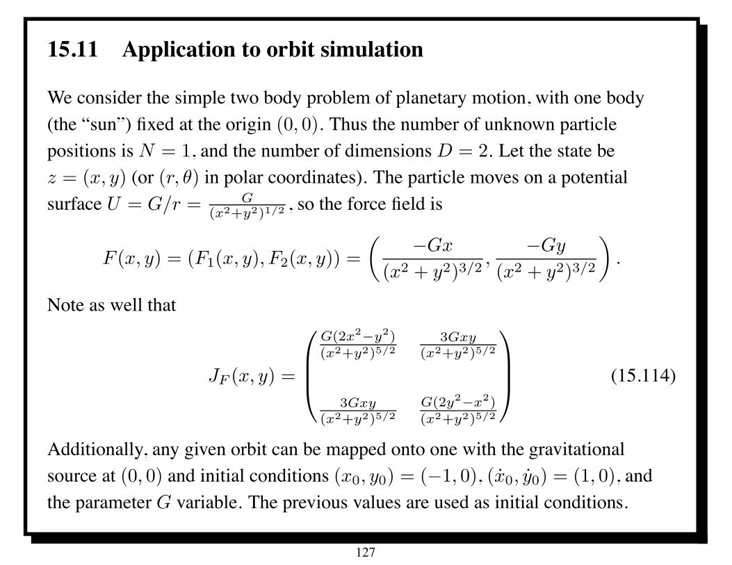
15.11 Application to orbit simulation
We consider the simple two body problem of planetary motion, with one body(the “sun”) fixed at the origin (0, 0). Thus the number of unknown particlepositions is N = 1, and the number of dimensions D = 2. Let the state bez = (x, y) (or (r, /) in polar coordinates). The particle moves on a potentialsurface U = G/r = G
(x2+y2)1/2 , so the force field is
F (x, y) = (F1(x, y), F2(x, y)) =
#!Gx
(x2 + y2)3/2,
!Gy
(x2 + y2)3/2
$.
Note as well that
JF (x, y) =
+
11,
G(2x2!y2)(x2+y2)5/2
3Gxy(x2+y2)5/2
3Gxy(x2+y2)5/2
G(2y2!x2)(x2+y2)5/2
-
22. (15.114)
Additionally, any given orbit can be mapped onto one with the gravitationalsource at (0, 0) and initial conditions (x0, y0) = (!1, 0), (x0, y0) = (1, 0), andthe parameter G variable. The previous values are used as initial conditions.
127
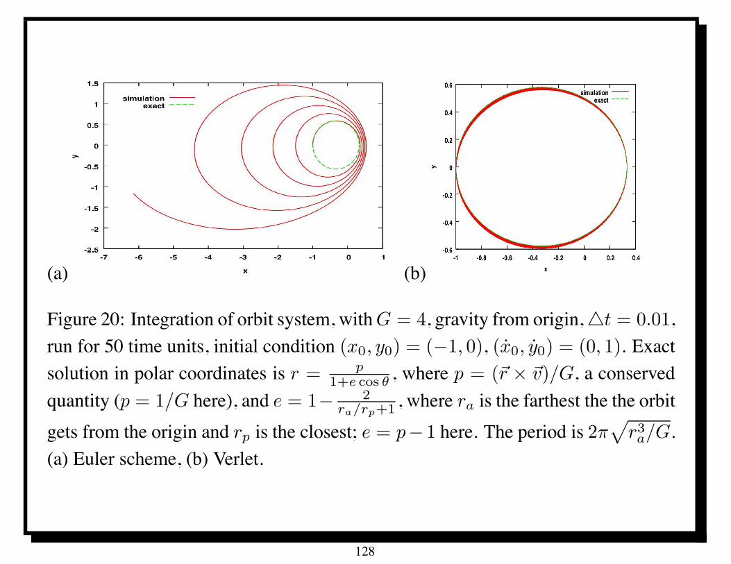
(a) (b)
Figure 20: Integration of orbit system, with G = 4, gravity from origin, 1t = 0.01,run for 50 time units, initial condition (x0, y0) = (!1, 0), (x0, y0) = (0, 1). Exactsolution in polar coordinates is r = p
1+e cos ( , where p = ((r # (v)/G, a conservedquantity (p = 1/G here), and e = 1! 2
ra/rp+1 , where ra is the farthest the the orbitgets from the origin and rp is the closest; e = p! 1 here. The period is 2#
8r3a/G.
(a) Euler scheme, (b) Verlet.
128
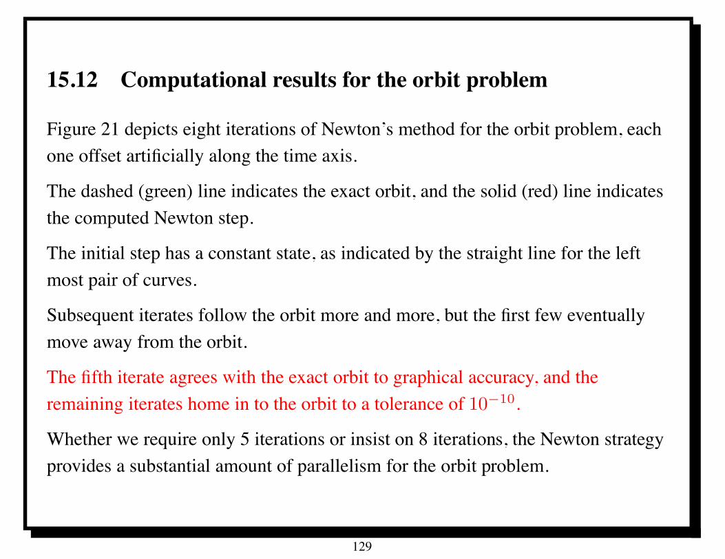
15.12 Computational results for the orbit problem
Figure 21 depicts eight iterations of Newton’s method for the orbit problem, eachone offset artificially along the time axis.
The dashed (green) line indicates the exact orbit, and the solid (red) line indicatesthe computed Newton step.
The initial step has a constant state, as indicated by the straight line for the leftmost pair of curves.
Subsequent iterates follow the orbit more and more, but the first few eventuallymove away from the orbit.
The fifth iterate agrees with the exact orbit to graphical accuracy, and theremaining iterates home in to the orbit to a tolerance of 10!10.
Whether we require only 5 iterations or insist on 8 iterations, the Newton strategyprovides a substantial amount of parallelism for the orbit problem.
129
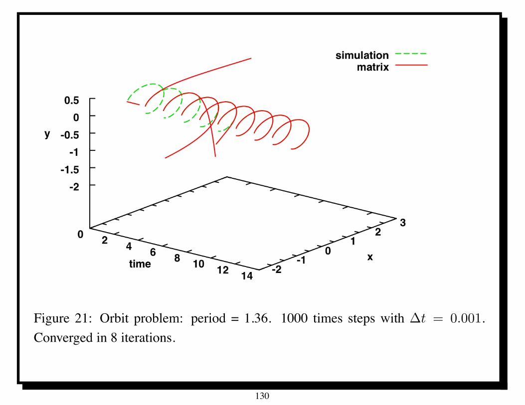
Figure 21: Orbit problem: period = 1.36. 1000 times steps with !t = 0.001.Converged in 8 iterations.
130
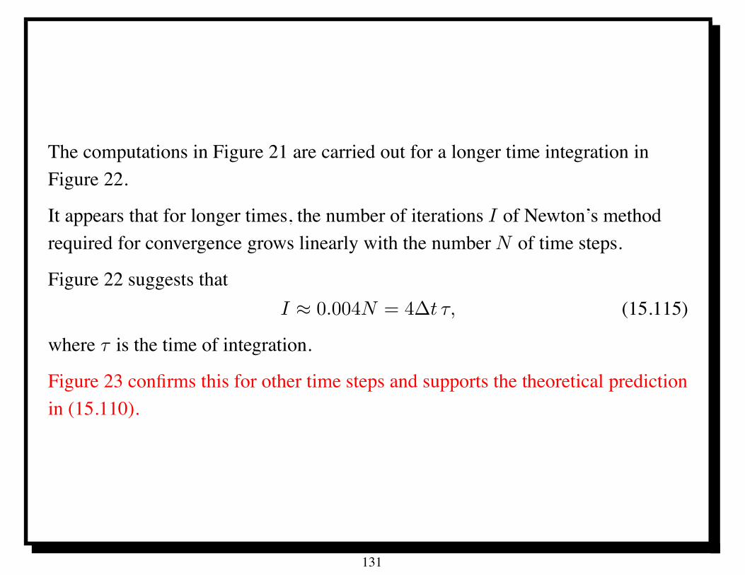
The computations in Figure 21 are carried out for a longer time integration inFigure 22.
It appears that for longer times, the number of iterations I of Newton’s methodrequired for convergence grows linearly with the number N of time steps.
Figure 22 suggests thatI " 0.004N = 4!t ,, (15.115)
where , is the time of integration.
Figure 23 confirms this for other time steps and supports the theoretical predictionin (15.110).
131
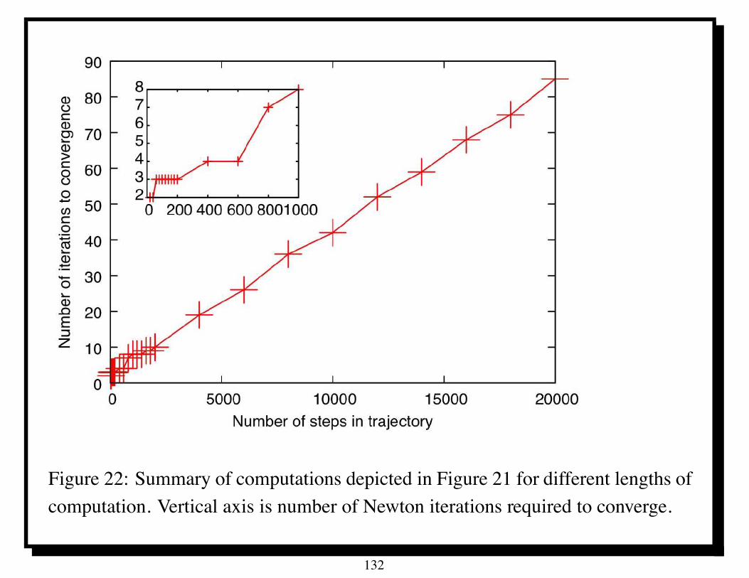
Figure 22: Summary of computations depicted in Figure 21 for different lengths ofcomputation. Vertical axis is number of Newton iterations required to converge.
132
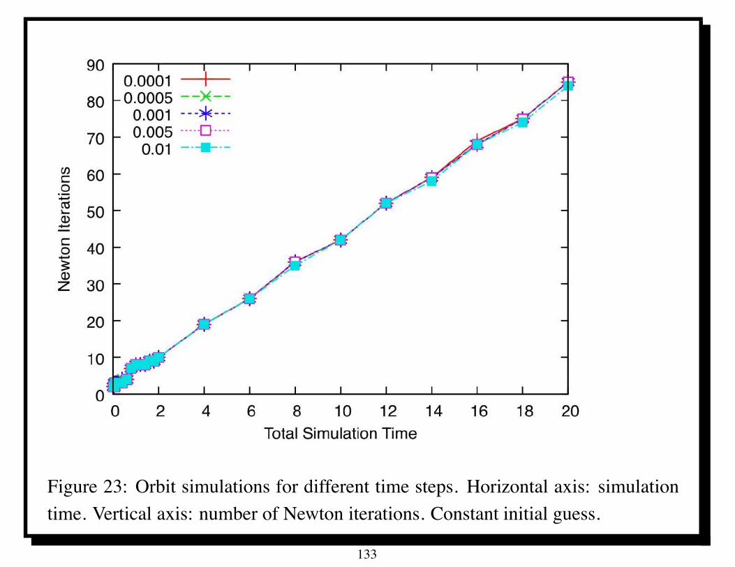
Figure 23: Orbit simulations for different time steps. Horizontal axis: simulationtime. Vertical axis: number of Newton iterations. Constant initial guess.
133
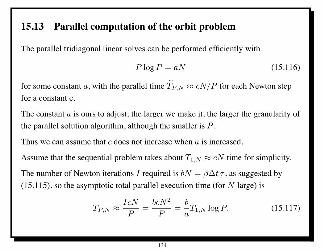
15.13 Parallel computation of the orbit problem
The parallel tridiagonal linear solves can be performed efficiently with
P log P = aN (15.116)
for some constant a, with the parallel time *TP,N " cN/P for each Newton stepfor a constant c.
The constant a is ours to adjust; the larger we make it, the larger the granularity ofthe parallel solution algorithm, although the smaller is P .
Thus we can assume that c does not increase when a is increased.
Assume that the sequential problem takes about T1,N " cN time for simplicity.
The number of Newton iterations I required is bN = $!t , , as suggested by(15.115), so the asymptotic total parallel execution time (for N large) is
TP,N " IcN
P=
bcN2
P=
b
aT1,N log P. (15.117)
134
15.14 Speedup of the orbit problem
This says that the speedup would be estimated by the relation
SP,N " a
b log P=
a
$!t ,. (15.118)
In particular, this says that the speedup can be arbitrarily large for fixed , as!t . 0.
On the other hand, (15.118) also says that the efficiency would be restricted by therelation
EP,N " a
bP log P=
1
bN=
1
I, (15.119)
consistent with the observation that our algorithm simply duplicates the sequentialalgorithm I times.
Note that the adjustable parameters (a and P ) drop out of the relation (15.119) forefficiency.
135
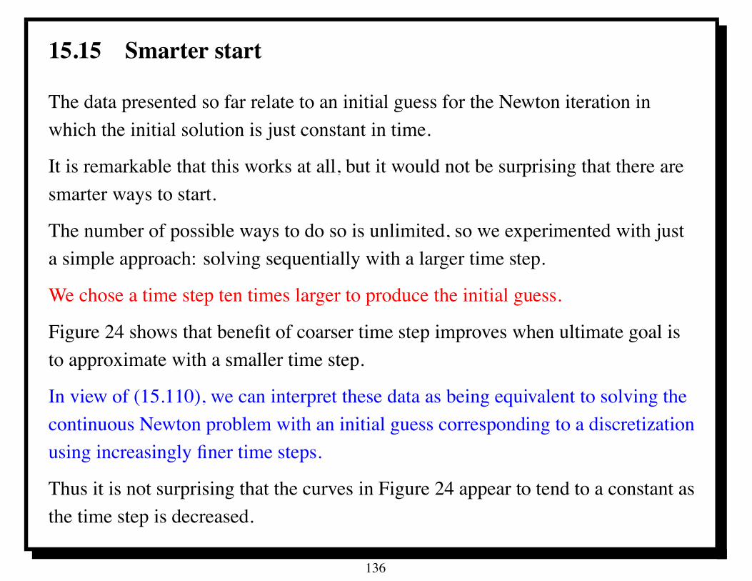
15.15 Smarter start
The data presented so far relate to an initial guess for the Newton iteration inwhich the initial solution is just constant in time.
It is remarkable that this works at all, but it would not be surprising that there aresmarter ways to start.
The number of possible ways to do so is unlimited, so we experimented with justa simple approach: solving sequentially with a larger time step.
We chose a time step ten times larger to produce the initial guess.
Figure 24 shows that benefit of coarser time step improves when ultimate goal isto approximate with a smaller time step.
In view of (15.110), we can interpret these data as being equivalent to solving thecontinuous Newton problem with an initial guess corresponding to a discretizationusing increasingly finer time steps.
Thus it is not surprising that the curves in Figure 24 appear to tend to a constant asthe time step is decreased.
136
Figure 24: Orbit simulations for different time steps. Horizontal axis: simulationtime. Vertical axis: number of Newton iterations. Initial guess is solution using a(ten-times) coarser time step.
137
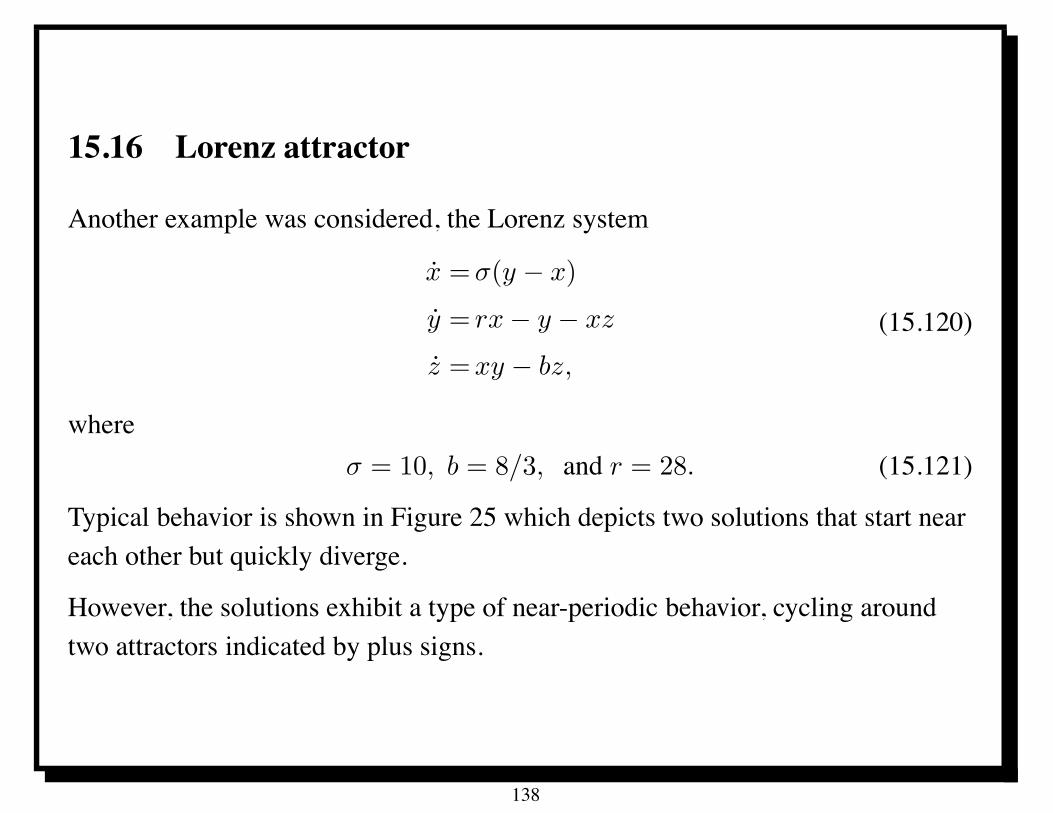
15.16 Lorenz attractor
Another example was considered, the Lorenz system
x =0(y ! x)
y = rx ! y ! xz
z =xy ! bz,
(15.120)
where0 = 10, b = 8/3, and r = 28. (15.121)
Typical behavior is shown in Figure 25 which depicts two solutions that start neareach other but quickly diverge.
However, the solutions exhibit a type of near-periodic behavior, cycling aroundtwo attractors indicated by plus signs.
138
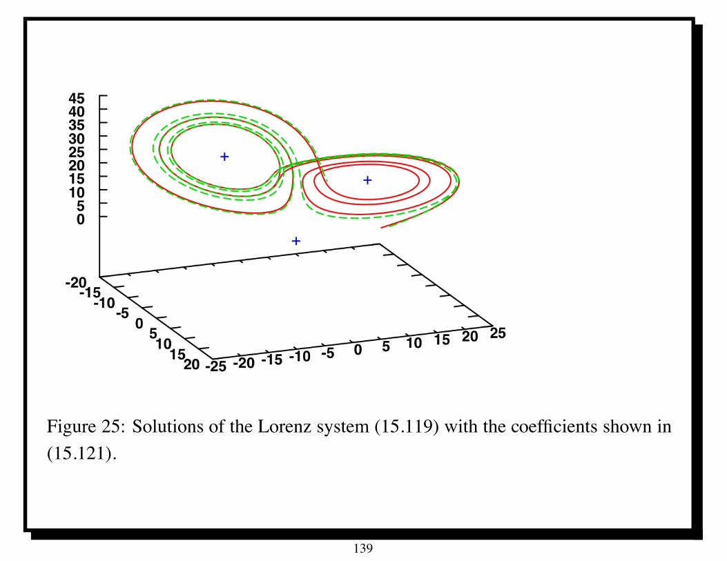
Figure 25: Solutions of the Lorenz system (15.119) with the coefficients shown in(15.121).
139
15.17 Lorenz attractor Newton parallelization
Figure 26 indicates the number of Newton iterations required to solve thedifference approximation to the Lorenz system (15.119) with the coefficientsshown in (15.121) using a constant initial guess.
Figure 27 indicates the number of Newton iterations required to solve thedifference approximation to the Lorenz system (15.119) with the coefficientsshown in (15.121) using a constant initial guess for various time steps.
We see confirmation of the prediction in (15.110).
Figure 28 indicates the decrease in the required number of Newton iterations tosolve the difference approximation to the Lorenz system (15.119) with thecoefficients shown in (15.121) using an nitial guess based on a (ten times) coarsertime step.
140
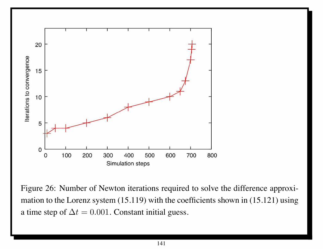
Figure 26: Number of Newton iterations required to solve the difference approxi-mation to the Lorenz system (15.119) with the coefficients shown in (15.121) usinga time step of !t = 0.001. Constant initial guess.
141
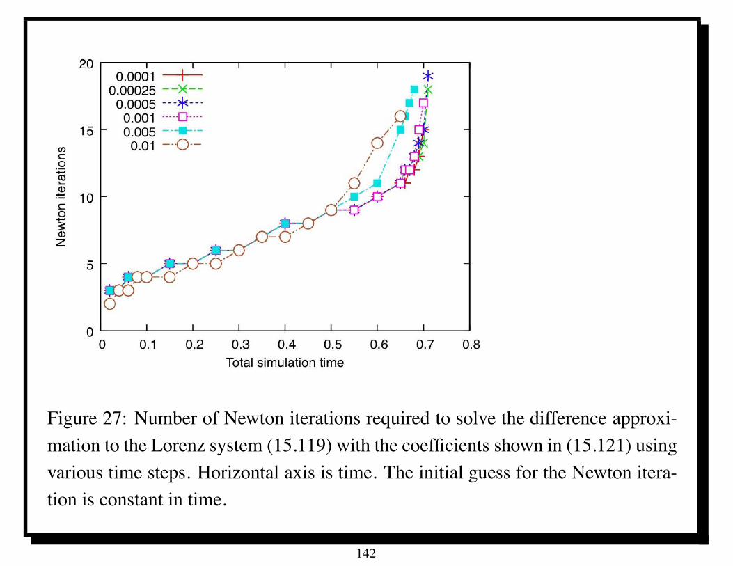
Figure 27: Number of Newton iterations required to solve the difference approxi-mation to the Lorenz system (15.119) with the coefficients shown in (15.121) usingvarious time steps. Horizontal axis is time. The initial guess for the Newton itera-tion is constant in time.
142
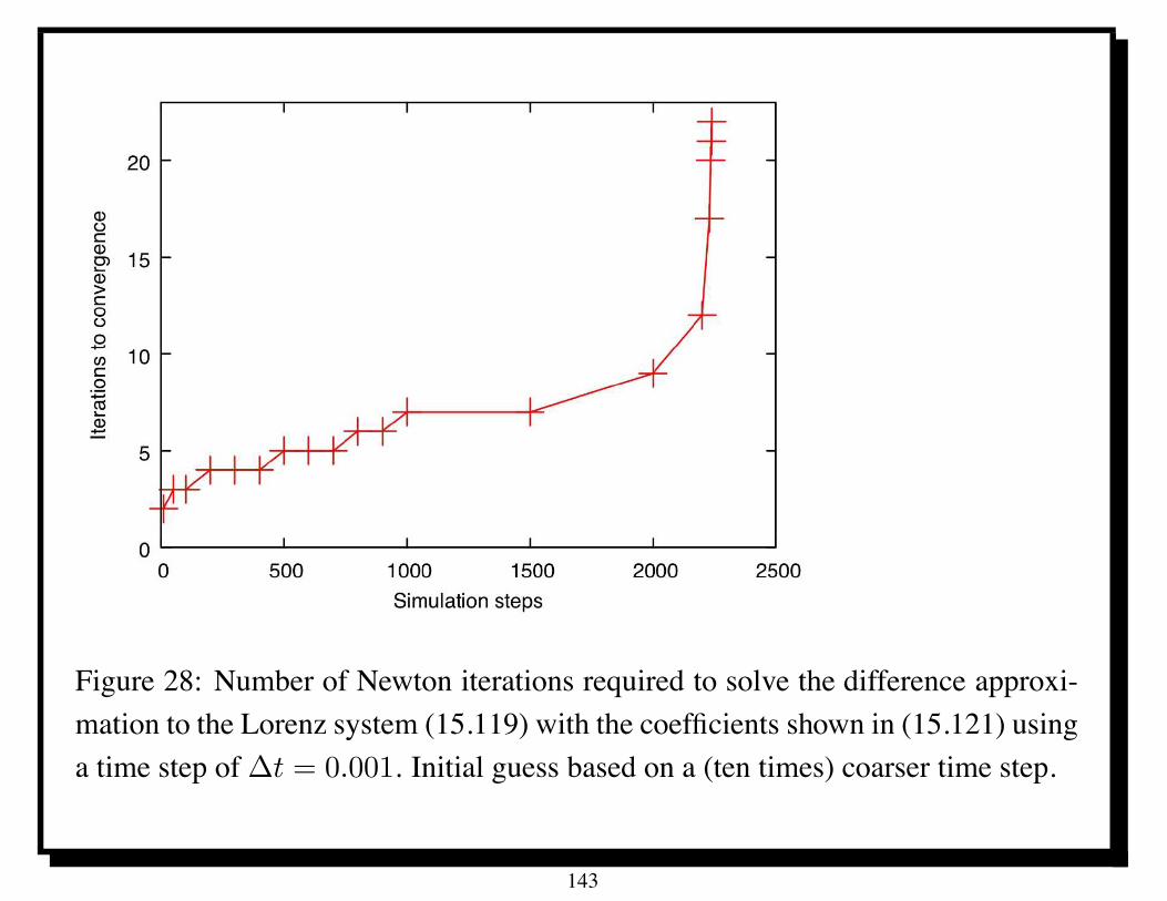
Figure 28: Number of Newton iterations required to solve the difference approxi-mation to the Lorenz system (15.119) with the coefficients shown in (15.121) usinga time step of !t = 0.001. Initial guess based on a (ten times) coarser time step.
143
15.18 Other approaches
Many high-order methods have been proposed that exhibit parallelism in thehigh-order steps [2].
“Parareal” methods provide efficient parallelizations of non-linear, time-dependentproblems via domain decomposition in the time domain [1, 13, 14].
• One limitation is the inclusion of a serial section which plays the role of apreconditioner.
• Techniques presented here can be integrated with those of [1, 13, 14] topotentially improve scalability.
• The techniques here may provide a scalable parallel algorithm for this or asimilar preconditioner.
144
15.19 Conclusions (and Perspectives)
We have demonstrated that the Newton parallel method can provide significantspeedup for solving ODE’s.
The efficiency is limited by the number of required Newton iterations, but thespeedup can be arbitrarily large as the time step is decreased.
The main reason that efficiency is limited by the number of required Newtoniterations for the problems considered here is that we focused on explicittime-stepping schemes.
Thus the sequential algorithm gets replicated in each Newton iteration.
But for problems requiring implicit time-stepping schemes, a Newton (or similar)iteration might be required even in the sequential case.
In this scenario, the efficiency might be significantly better.
145
15.20 (Conclusions and) Perspectives
The Newton parallel method benefits greatly from a good initial guess.
What is the best way to use P processors to collectively approximate a solution toan ODE?
• Sounds like original question but now Newton parallel method computesrefinement, so initial step need not be convergent.
• One idea: each processor solves slightly different problems and then we usethis data to synthesize an approximation.
• Something like the data assimilation problem?
Applying these ideas to ODE’s arising from the semi-discretization of PDE’s willbe a significant challenge.
• Molecular dynamics is typically done with explicit time-stepping methods(e.g., Verlet)
• flow problems (Navier-Stokes) often involve implicity methods (Euler orbackward differentiaion) [10].
146
References
[1] L. Baffico, S. Bernard, Y. Maday, G. Turinici, and G. Zerah. Parallel-in-timemolecular-dynamics simulations. Phys. Rev. E, 66:057701, 2002.
[2] Kevin Burrage. Parallel and sequential methods for ordinary differentialequations. Oxford University Press, 1995.
[3] Terry Clark, Reinhard von Hanxleden, J. Andrew McCammon, andL. Ridgway Scott. Parallelization using decomposition for moleculardynamics. In Proceedings of the Scalable High-Performance ComputingConference, pages 95–102, Knoxville, Tennessee, May 1994. IEEEComputer Society Press.
[4] Xie Dexuan and L. R. Scott. An analysis of the parallel U-cycle multigridmethod. Research Report UC/CS TR-2010-03, Dept. Comp. Sci., Univ.Chicago, 2010.
[5] Y. Duan and P Kollman. Pathways to a protein folding intermediateobserved in a 1-microsecond simulation in aqueous solution. Science,282:740–744, 1998.
147
[6] G. A. Geist and C. H. Romine. LU factorization algorithms ondistributed-memory multiprocessor architectures. SIAM J. Sci. Stat.Comput., 9:639–649, 1988.
[7] John L. Gustafson, Gary R. Montry, and Robert E. Benner. Development ofparallel methods for a 1024-processor hypercube. SIAM J. Sci. Stat. Comp.,9(4), 1988.
[8] A. Ilin and L. R. Scott. Loop splitting for superscalar architectures. J.Supercomp. Appl. and High Perf. Computing, 10:336–340, 1996.
[9] E. Isaacson and H. B. Keller. Analysis of Numerical Methods. John Wileyand Sons, New York, 1966.
[10] Hector Juarez, L. R. Scott, R. Metcalfe, and B. Bagheri. Direct simulation offreely rotating cylinders in viscous flows by high–order finite elementmethods. Computers & Fluids, 29:547–582, 2000.
[11] A. Karp. Gordon Bell Prize for 1997. NA Digest, 97(12):226–319, March1997.
[12] F. Thomson Leighton. Introduction to Parallel Algorithms and
148
Architectures: Arrays, Trees, and Hypercubes. Morgan Kaufmann, SanMateo, CA, 1992.
[13] Jacques-Louis Lions, Yvon Maday, and Gabriel Turinici. Resolution d’EDPpar un schema en temps “parareel”. C. R. Acad. Sci. Paris, 332(7):661–668,2001.
[14] Yvon Maday and Gabriel Turinici. A parareal in time procedure for thecontrol of partial differential equation. C. R. Acad. Sci. Paris,335(4):387–392, 2002.
[15] U. Schendel. Introduction to numerical methods for parallel computers.Chichester: Ellis Horwood Limited, 1984.
[16] L. R. Scott, T. W. Clark, and B. Bagheri. Scientific Parlallel Computing.Princeton University Press, 2005.
[17] L. R. Scott and Dexuan Xie. The parallel u-cycle multigrid method. InProceedings of the 8th Copper Mountain Conference on Multigrid Methods,April 6-11, 1997, 1997.
[18] D. P. Siewiorek, C. G. Bell, and A. Newell. Computer Structures: Principles
149
and Examples. New York: McGraw-Hill, 1982.
150