On Bias, Variance, 0/1—Loss, and the Curse-of …sushil/class/ml/papers/local/curseDim.pdf · and the Curse-of-Dimensionality ... “training” sample T Dfxi;yigN 1 ... wisdom

P1: RPS/TKL P2: RPS/TKL QC: RPS

Data Mining and Knowledge Discovery KL411-03-Friedman February 25, 1997 17:15

Data Mining and Knowledge Discovery 1, 55–77 (1997)c© 1997 Kluwer Academic Publishers. Manufactured in The Netherlands.

On Bias, Variance, 0/1—Loss,and the Curse-of-Dimensionality

JEROME H. FRIEDMANDepartment of Statistics and Stanford Linear Accelerator Center, Stanford University

Editor: Usama Fayyad

Received June 3, 1996; Revised October 23, 1996; Accepted October 23, 1996

Abstract. The classification problem is considered in which an output variabley assumes discrete values withrespective probabilities that depend upon the simultaneous values of a set of input variablesx = {x1, . . . , xn}. Atissue is how error in the estimates of these probabilities affects classification error when the estimates are used ina classification rule. These effects are seen to be somewhat counter intuitive in both their strength and nature. Inparticular the bias and variance components of the estimation error combine to influence classification in a verydifferent way than with squared error on the probabilities themselves. Certain types of (very high) bias can becanceled by low variance to produce accurate classification. This can dramatically mitigate the effect of the biasassociated with some simple estimators like “naive” Bayes, and the bias induced by the curse-of-dimensionalityon nearest-neighbor procedures. This helps explain why such simple methods are often competitive with andsometimes superior to more sophisticated ones for classification, and why “bagging/aggregating” classifiers canoften improve accuracy. These results also suggest simple modifications to these procedures that can (sometimesdramatically) further improve their classification performance.

Keywords: classification, bias, variance, curse-of-dimensionality, bagging, naive Bayes, nearest-neighbors

1. Introduction

One of the most common and important uses for data is prediction. The purpose is to predict(forecast) the unknown value of some attributey of a system (“output” or “response”variable), based on the known values of other attributesx = (x1, . . . , xn) (“input” or“predictor” variables). With the “supervised learning” paradigm the data base provides a“training” sample

T = {xi , yi }N1 (1.1)

of previously solved cases in which both the values of the inputs and corresponding outputshave been recorded. The goal of a “learning” algorithm is to use this data (1.1) to constructa reliable rule for predicting likely output valuesy for future data where only the values ofthe inputsx have been recorded.

The rule construction strategy can depend upon the nature of the output variable interms of the types of values it can realize. The two most common data types are orderabley∈ R1 (“regression”) and categoricaly ∈ {y1, . . . , yL} (“classification”). With an orderablevariable there is an order relation between every pair of its valuesy, y′(y ≤ y′ or y > y′)and a distance|y − y′| defined between them. For a categorical variable there exists no



56 FRIEDMAN

order relation nor a continuous distance between its values. Two values are either equal(y = y′) or they are unequal (y 6= y′).

Historically, both regression and classification have been developed from the commonperspective of real valued prediction. In the case of classification the real valued (surrogate)outputs are taken to be the respective probabilities thaty realizes each of its individualvalues, as a function of the input valuesx. These probabilities are then used in a decisionrule to forecast the most likely (categorical) value for the outputy. Much research inclassification has been devoted to achieving higher accuracy probability estimates underthe presumption that this will generally lead to more accurate (categorical) prediction. The(often counter intuitive) results obtained in this paper challenge that presumption. Moreaccurate probability estimates do not necessarily lead to better classification performanceand often can make it worse.

This has implications concerning applications of classification as well as for future di-rections of methodological research. In individual applications one is faced with the choiceof which method(s) to consider. Often older simpler techniques are discarded in favor ofnewly developed sophisticated methods on the grounds that the latter can provide moreaccurate estimates of the probabilities of the respective output values. Results derived inthis paper show that, even if this is the case, it need not result in smaller classification error.Very simple procedures such as “naive” Bayes and nearest neighbor methods generallyprovide very poor probability estimates especially in high dimensional settings involvingmany input variables. Never-the-less they often yield lower prediction error than other(newer) methods intended to produce higher accuracy estimates of the probabilities. Theresults derived in this paper indicate those situations in which this is likely to occur. Theyalso suggest straightforward modifications to these “simple” procedures that can sometimesimprove their classification performance even more, by selectively further reducing the ac-curacy of their probability estimates. In terms of methodological research these resultssuggest that in situations where the goal is accurate classification, focusing on improvedprobability estimation may be misguided and a totally different paradigm may be required.

2. Classification

As noted above, in the classification problem the output variabley assumes values on anunordered discrete sety ∈ {y1, . . . , yL}. In this paper the special (but common) case inwhich L = 2 is considered. Although many of the concepts generalize to the more generalcaseL ≥ 3, the derivations and underlying intuition are more straightforward for this special(“two-class”) case. As will be seen, even in this restricted setting much of the conventionalwisdom concerning the classification problem can be brought into question.

Without loss of generality we takey ∈ {0, 1}. The goal of a classification procedure is topredict the output value given the values of a set of “input” variablesx = {x1, . . . , xn} simul-taneously measured on the same system. It is often the case that at a particular pointx∈ Rn

the value ofy is not uniquely determinable. It can assume both its values with respectiveprobabilities that depend on the location of the pointx in then-dimensional input space

Pr(y = 1 | x) = 1− Pr(y = 0 | x) .= f (x). (2.1)



ON BIAS, VARIANCE, 0/1—LOSS, AND THE CURSE-OF-DIMENSIONALITY 57

Here f (x) is a single valued deterministic function that at every pointx ∈ Rn specifies theprobability thaty assumes its second value.

The role of a classification procedure is to produce a rule that makes a predictiony(x) ∈{0, 1} for the correct class labely at every input pointx. The goal is to choosey(x) tominimize inaccuracy as characterized by the misclassification “risk” (expected or averageloss)

r (x) = l1 f (x)1(y(x) = 0)+ l0(1− f (x))1(y(x) = 1). (2.2)

Herel0 andl1 are the losses incurred for the respective misclassifications,f (x) is given by(2.1), and 1(·) is an indicator function of the truth of its argument

1(η) ={

1 if η is true0 otherwise.

(2.3)

The misclassification risk (2.2) is minimized by the (“Bayes”) rule

yB(x) = 1

(f (x) ≥ l0

l0+ l1

)(2.4)

which (by definition) achieves the lowest possible risk

r B(x) = min(l1 f (x), l0(1− f (x)). (2.5)

Note that the rule (2.4) is not necessarily the only minimizer of (2.2). Other rules may alsoachieve minimum risk (2.5). Also, in the special (but common) casel0 = l1 = 1, (2.4)reduces to predicting the most probable class and (2.5) represents the fraction of erroneouspredictions thereby encountered.

Generally the functionf (x) (2.1) characterizing a particular system is unknown. How-ever, data from the system is available in the form of a collection of previously solved casesin which both the input and output variables have been measured. This “training” dataset (1.1) is used to “learn” a classification ruley(x | T) for (future) prediction. The usualparadigm for accomplishing this is to use the training dataT (1.1) to form an approximation(estimate)f (x | T) to f (x) (2.1) and substitute this into (2.4)

y(x | T) = 1

(f (x | T) ≥ l0

l0+ l1

). (2.6)

When f (x) 6= f (x) this rule (2.6) may be different than from the Bayes rule (2.4) and thusnot achieve the minimal Bayes risk (2.5). It is the purpose of this study to examine the wayin which inaccuraciesf (x)− f (x) in the function estimate are reflected in misclassificationrisk.



58 FRIEDMAN

3. Function estimation

In the usual function estimation setting one assumes that an output variabley is related toa set of input variablesx by

y = f (x)+ ε (3.1)

where f (x) (“target function”) is a single valued deterministic function ofn arguments andε is a random variable distributed according to some lawε ∼ L(ε | x). By definition itsaverageE(ε | x) = 0 for all x so that the target function is defined by

f (x) = E(y | x). (3.2)

The goal is to obtain an estimate

f (x | T) = E(y | x, T) (3.3)

using a training data setT (1.1). Inaccuracy is usually quantified by root-mean-squaredprediction error

rms(x) = E1/2ε [(y− f (x | T))2] (3.4)

where the expected value in (3.4) is taken with respect to the distribution ofε (3.1).The classification problem can be cast in this function estimation setting by observing

that (3.2) holds fory and f (x) in (2.1) so that they can be related by (3.1) withε distributedas a (centered) binomial distribution with variance var(ε | x) = f (x)(1 − f (x)). Thus,regular function estimation technology (3.3) can be applied to obtain the estimatef (x | T),which is plugged into (2.6) to form a classification rule. This is the paradigm used by manypopular classification methods including neural networks (Lippmann, 1989), decision treeinduction methods (Breiman et al., 1984; Quinlan, 1993), projection pursuit (Friedman,1985), and nearest neighbor methods (Fix and Hodges, 1951).

4. Density estimation

An alternative paradigm for estimatingf (x) (2.1) in the classification setting is based ondensity estimation. Here Bayes theorem

f (x) = π1 p1(x)π0 p0(x)+ π1 p1(x)

(4.1)

is applied where{pj (x) = Pr(x | y = j )}10 are the class conditional probability densityfunctions and{π j = Pr(y = j )}10 are the unconditional (“prior”) probabilities of each class.The training data (1.1) are partitioned into subsetsT = {T0, T1} with the same class label.The data in each subset are separately used to estimate its respective probability density




{ pj (x | Tj )}10. These estimates are plugged into (4.1) to obtain an estimatef (x | T) whichis in turn plugged into (2.6) to form a classification rule. Examples of this approach arediscriminant analysis (see McLachlan, 1992), kernel discriminant methods (Hand, 1982),Gaussian mixtures (Chow and Chen, 1992), learning vector quantization techniques (Ko-honen, 1990), and Bayesian belief networks (Heckerman et al., 1994).

5. Bias, variance, and estimation error

Whether one applies the function estimation (3.3) or density estimation (4.1) approach,the estimated probabilityf (x | T) depends upon the training dataT (1.1) used to obtainit. A change in the data (usually) results in a change in the probability estimate at (atleast) some of the input pointsx. In most applications the training data set (1.1) representsa random sampling from the system under study. Even if the target probability functionf (x) is everywhere stationary, sampling the system at different times results in (at leastsomewhat) different training data setsT and thereby different estimatesf (x | T). For agiven set of input points{xi }N1 the corresponding outputs{yi }N1 are random owing to thestochastic componentε (3.1), and generally the input points themselves represent a randomsampling (observational study).

The random nature of the training dataT implies that the estimatef (x | T) is a randomvariable that assumes a distribution of values at each input pointx governed by some(usually unknown) probability lawf (x) ∼ L( f | x) characterized by a probability densityfunction p( f | x). Estimating f (x) with a particular training data setT gives rise to aparticular random realization off (x | T) with relative probabilityp( f | x). Two importantparameters of any such distribution are its first two moments, the mean (expected value)

E f (x) =∫ ∞−∞

f p( f | x) d f (5.1)

and variance

var f (x) =∫ ∞−∞( f − E f (x))2 p( f | x) d f . (5.2)

Both of these quantities directly affect expected prediction error (3.4) through the wellknown decompositions

ET [y− f (x | T)]2 = ET [ f (x)− f (x | T)]2+ Eε[ε | x]2 (5.3)

and

ET [ f (x)− f (x | T)]2 = [ f (x)−ET f (x | T)]2+ET [ f (x | T)−ET f (x | T)]2. (5.4)

The left side of (5.3) represents the squared prediction error (atx) averaged over repeatedlyrealized training samples of the (same) sizeN from the system under study. The last term



60 FRIEDMAN

in (5.3) is independent of both the target function and the training sample and reflects theirreducible prediction error due to the random nature of the output variable (2.1), (3.1). Theother term in (5.3) is the squared “estimation error” in the target functionf (x) averagedover training samples. This depends onf (x) and the method used to obtainf (x | T). From(5.4) one sees that this quantity depends only on the mean (5.1) and the variance (5.2) ofthe distribution of f (x | T). The last quantity in (5.4) is just the variance (5.2). The otherquantity in (5.4) is the square of the “bias”

bias f (x) = f (x)− E f (x ). (5.5)

The variance (5.2) reflects the sensitivity of the function estimatef (x | T) to the trainingsampleT . Less sensitivity means that the estimate will be more stable against changes(sampling variations) in the data and thus be less variable under repeated sampling. Thebias (5.5) reflects sensitivity to the target functionf (x). It represents how closely on averagethe estimate is able to approximate the target. From (5.4) one sees that it is desirable to haveboth low bias-squared and low variance since both contribute to the squared estimation errorin equal measure. There is however a tension between these goals (Geman et al., 1992).The purpose of training is to gain information concerning the target function from the data;therefore sensitivity to the training data is essential, and generally more sensitivity results inlower bias. However, this in turn increases variance and so there is a natural “bias-variancetrade-off” associated with function approximation.

For a given bias (5.5) the variance (5.2) generally decreases with increasing trainingsample sizeN (1.1). Therefore for problems with large training samples the bias can be thedominant contributor to estimation error. Since larger and larger data bases are becomingroutinely available, most modern research in learning methodology has focused on increas-ingly flexible techniques that reduce estimation bias, some with considerable success. From(5.3), (5.4) one can see that this is a reasonable strategy for function approximation (basedon root-mean-squared error (3.4)), provided enough attention is paid to the variance (“over-fitting”). For classification however this strategy has been less successful in improvingperformance. Some simple highly biased procedures such as “naive” Bayes (Good, 1965)and nearest neighbor methods (Fix and Hodges, 1951) remain competitive with and some-times outperform more sophisticated ones, even with moderate to large training samples(Holte, 1993). In the next section we show that this may not be as surprising as it seems.The quantitiesE f (x) (5.1) and varf (x) (5.2) that characterize the distribution off (x | T)conspire to affect classification error in a very different way whenf (x | T) is used in aclassification rule (2.6).

6. Bias, variance, and classification error

For concreteness we takel0 = l1 = 1 in (2.4), (2.6) so that the threshold in the indicatorfunction is 1/2 and misclassification risk (2.2) reduces to probability of misclassificationPr(y(x) 6= y). The first step in uncovering howE f (x) (5.1) and varf (x) (5.2) affectclassification error is to decompose it into the irreducible error associated with the randomnature ofy (2.1), (3.1) and a reducible part that depends onf (x) (3.3) in analogy with




(5.3) for squared-error loss. Given a particular training sampleT (1.1) the error ratePr(y(x | T) 6= y) (averaged over all future predictions atx) depends on whether or not thedecision (2.6) agrees with that of the Bayes rule (2.4). If it does then its error rate is theirreducible error associated with the Bayes rule (2.5) Pr(y(x | T) 6= y) = Pr(yB(x) 6= y) =min[ f (x), 1− f (x)]. If not, then it suffers an increased error rate Pr(y(x | T) 6= y) =max[ f (x), 1− f (x)] = |2 f (x)− 1| + Pr(yB(x) 6= y). Therefore one has

Pr(y(x | T) 6= y) = |2 f (x)− 1| 1[y(x | T) 6= yB(x)] + Pr(yB(x) 6= y). (6.1)

Averaging over all training samplesT (of sizeN), under the assumption that they are drawnindependently of future data to be predicted, one has

Pr(y 6= y) = |2 f − 1| Pr(y 6= yB)+ Pr(yB 6= y). (6.2)

Here (6.2) and in what follows all quantities are presumed to be conditioned at a particularpointx in the input space, and that explicit dependence is suppressed for convenience.

From (6.2) one sees that the classification error rate Pr(y 6= y) is linearly proportionalto Pr(y 6= yB) which is the only quantity in (6.2) that involves the probability estimatefthrough (2.6). It can be viewed as a decision “boundary” error in that it represents mises-timation of the (optimal) decision boundary separating the two classes in the input space,defined by the set of points (surface) for whichf (x) = 1/2. This “boundary error” is theanalog of the (squared) estimation errorE[ f (x)− f (x)]2 in (5.3) and (5.4).

In order to proceed further it is necessary to calculate how the boundary error dependson the distribution off , p( f ), induced by the random variations in training data setsT as(repeatedly) sampled from the system under study. This is just the tail area ofp( f ) on theopposite side of the value 1/2 from the true probabilityf

Pr(y 6= yB) = 1( f < 1/2)∫ ∞

1/2p( f ) d f + 1( f ≥ 1/2)

∫ 1/2

−∞p( f ) d f . (6.3)

This will depend on the detailed form of the distributionp( f ), and not just on its first twomoments (5.1), (5.2), as was the case with squared estimation error (5.4). In order to gainsome intuition we approximatep( f ) by a normal distribution

p( f ) = 1√2πvar f

exp

(−1

2

( f − E f )2

var f

). (6.4)

This approximation is often reasonable since for many procedures the computation off involves a (sometimes complex) averaging process. Even when it is not the case thequalitative conclusions are still generally valid. Assuming (6.4) the boundary error (6.3)becomes

Pr(y 6= yB) = 8[

sign( f − 1/2)E f − 1/2√

var f

](6.5)



62 FRIEDMAN

where

8(z) = 1√2π

∫ ∞z

e−12 u2

du (6.6)

is the upper tail area of the standard normal distribution.

7. Discussion

Inspection of (6.5) reveals that the boundary error depends upon the true probabilityf , andthe systematic component of the estimateE f , through

b( f, E f ) = sign(1/2− f )(E f − 1/2). (7.1)

For any (nonzero) value of the random component, varf > 0, the boundary error ratePr(y 6= yB) is monotonically increasing inb( f, E f ). In this sense it can be viewed as ananalog of the estimation bias (5.5) squared for squared-error loss (5.4). For conveniencewe refer tob( f, E f ) (7.1) as the “boundary bias”. (In cases wherep( f ) is an asymmetricdistribution it is more natural to define boundary bias (7.1) in terms of the median insteadof the meanE f .)

Comparison of (6.2), (6.5) with (5.3), (5.4) reveals that the quantitiesE f and varf affectclassification error very differently than they affect estimation error on the probabilityfitself. For a given varf , estimation (squared) error (5.4) is proportional to the (squared)distance( f −E f )2 (bias-squared). In classification (6.2), (6.5) the dependence onf is onlythrough the sign off − 1/2, and the relevant quantity is boundary bias (7.1). Therefore,so long as boundary bias is negativeb( f, E f ) < 0 classification error decreases withincreasing|E f −1/2| irrespective of the estimation bias( f − E f ). For positive boundarybias the classification error increases with the distance ofE f from 1/2.

For a given value ofE f , estimation (squared) error (5.4) is proportional to varf . Forclassification error the effect of the varf depends mostly on the sign of the boundary bias(7.1). For a negative sign classification error decreases with decreasing variance (though notlinearly), whereas for a positive sign the error rateincreaseswith decreasing variance. Therate of increase/decrease depends on the absolute boundary bias. With estimation error (5.4)small variance does not necessarily provide small error; the bias-squared might be quitelarge. For classification, zero variance results in optimal classification (Bayes rule) irrespec-tive of the value of the estimation bias (5.5) provided boundary bias (7.1) is negative. For pos-itive boundary bias, zero variance gives rise to maximal error rate (certain boundary error) atx. Note that imposing the constraint 0≤ f (x) ≤ 1, while often improving estimation bias,need not improve boundary bias. In fact, it could increase boundary bias and thereby bound-ary error (6.5) unless a requisite reduction in variance is achieved through the constraint.

The “bias-variance trade-off” is clearly very different for classification error than estima-tion error on the probability functionf itself. The dependence of squared estimation error(5.4) on E f and varf is additive (bias-squared plus variance) whereas for classificationerror (6.2), (6.5) there is a strong (multiplicative) interaction effect. The effect of boundarybias (7.1) on classification error (6.2), (6.5) can be mitigated by low variance. Similarly,the affect of the variance depends on the value (especially the sign) of the boundary bias.




Therefore low variance (5.2) can be very important for classification but low (estimation)bias (5.5) squared is not. For the most part, all that is required ofE f is to insure that itbe on the same side of the value 1/2 as f (negative boundary bias). This being the case,one can reduce classification error toward its minimal (Bayes) value by reducing variancealone. In this sense variance tends to dominate bias for classification.

This different “bias-variance trade-off” for classification error (6.5) suggests that certainmethods that are inappropriate for function estimation because of their very high bias (5.4),(5.5) may none-the-less perform well for classification when their (highly biased) estimatesare used in the context of a classification rule (2.6). All that is required is predominatelynegative boundary bias (7.1) and small enough variance. Among these are procedures forwhich the bias is caused by “over-smoothing”; the estimate at each pointx, f (x), tends tobe shrunk towards the mean output value

y = 1

N

N∑i=1

yi . (7.2)

That is, the result of applying the procedure tends to be

f (x) = (1− α(x)) f (x)+ α(x)y (7.3)

where 0≤ α(x) ≤ 1 represents an “over-smoothing” coefficient that usually depends onx. The larger the value forα(x) the more over-smoothing bias. So long asy = 1/2 (equalnumber of each class in the training sample) then boundary bias is negative (for allx) andvar f (x) is likely to dominate classification error for such procedures. (Generalization toy 6= 1/2 is discussed in Section 10.) The variance is also controlled by the degree of (over)smoothing-more smoothing less variance. Therefore, the optimal amount of smoothing forminimizing classification error (6.2), (6.5) is likely to be much larger than that for estimationerror (5.4) since the latter is more strongly affected by estimation bias (5.5).

8. “Naive” Bayes methods

The naive Bayes approach is surprisingly effective (Titterington et al., 1981; Langley et al.,1992) given the crude nature of its approximation. It uses the density estimation paradigm(Section 4) and approximates each class conditional probability density{pk(x)}10 (4.1) bythe product of its marginal densities{p(k)j (xj )}nj=1 on each input variable,

pk(x) =n∏

j=1

p(k)j (xj ) (8.1)

with

p(k)j (xj ) =∫

pk(x)∏l 6= j

dxl . (8.2)

Data from each classk ∈ {0, 1}, and each input variablej ∈ {1, 2, . . . ,n}, are separatelyused to obtain corresponding estimatesp(k)j (xj ) of (8.2). These are used in (8.1), which is



64 FRIEDMAN

in turn plugged into (4.1) to form an estimate off (x). This is then inserted into (2.6) toproduce an output estimate.

Estimatesf (x) obtained in this manner are clearly biased (5.5) estimates off (x) (2.1),(3.1), even if the true marginal densities (8.2) are used, unless the input variables for everyclass happen to be totally independent. Since such total independence is far from beingrealized in most applications, this bias can be quite large, especially when there are manyinputs. Introducing estimates for (8.2) can introduce further bias and, of course, varianceas well.

The high degree of bias (5.4), (5.5) associated with the naive Bayes method (8.1), (8.2)makes it generally unsuitable for accurately approximating the target probability functionf (x) (2.1), (3.1). However, this bias is generally of the “over-smoothing” variety discussedin Section 7. The approximating densitiespk(x) tend to be much smoother than the corre-sponding (true) densitiespk(x) from which they are derived. They place substantive massover broader regions of the input space as evidenced by the fact that the entropy ofpk(x)is (usually much) greater than that ofpk(x). This over-smoothing of the class conditionaldensities produces an over-smoothed estimate off (x) when inserted into (4.1), producing(usually large) estimation bias (5.5), and therefore error (5.4). However, as discussed inSection 7, the boundary bias (7.1) produced by this mechanism is likely to remain negativeover much of the input space so that low variance estimates of the marginal densities (8.2)can produce low boundary error (6.5). This fact may explain why the naive Bayes methodhas seen so much success in classification despite its “naive” approach.

9. K-nearest neighbor methods

Another class of highly biased estimation procedures are those based onK -nearest neigh-bors. A local subregionR(x) ⊂ Rn of the input space, centered at the estimation pointx, is constructed and the target function estimate is taken to be the average of the trainingsample output values (1.1) in that region

f (x) = avexi∈R(x)yi . (9.1)

The predicting regionR(x) is defined to be the subregion of the input space containing theK closest training points tox

R(x) = {x′| ‖x− x′‖ ≤ d(K )} (9.2)

whered(K ) is theK th order statistic of{‖ x− xi ‖}N1 . This method requires the definition ofa distance‖x− x′‖ on the input space. This is usually taken to be a (weighted)lq distance

‖x− x′‖ =[

n∑j=1

|w j (xj − x′j )|q]1/q

(9.3)

with q = 2 (Euclidean distance) the most common choice. The weights{w j }n1 are usuallychosen to be inversely proportional to the (global) scales of the respective input variablesso as to give each input equal influence in defining the region (9.2).




ForK -nearest neighbor procedures the bias-variance trade-off associated with estimationerror generally is driven by the bias (5.5) in high dimensional settings (many inputs). Thisis due to the geometry of Euclidean spaces; the radius of a region varies as thenth root of itsvolume, whereas the number of training points in the regionK varies roughly linearly withthe volume. Thus, even the smallest possible volume (K = 1) gives rise to large regions interms of radius. This can already produce high bias even for the largest variance (K = 1).This phenomenon is referred to as the “curse-of-dimensionality” (Bellman, 1961).

Like naive Bayes (Section 8), the bias (5.5) associated withK -nearest neighbor pro-cedures is produced by over-smoothing. In fact, asK → N, f (x) → y (7.2) for all x.Providedy = 1/2 the boundary bias generally tends to be negative, and decreasing thevariance can have dramatic impact on reducing boundary error (6.5).

This is illustrated with a simple example. The input space is taken to be then-dimensionalunit hypercubex ∈ [0, 1]n. The class densities are

p0(x) = 2 · 1(x1 < 1/2), p1(x) = 2 · 1(x1 ≥ 1/2) (9.4)

so that the target probability function is

f (x) = 1(x1 ≥ 1/2). (9.5)

The prior probabilities (4.1) are taken to be equal (π0 = π1). This target (9.5) is a simplefunction ofx1 only, so having additional inputs serves to increaseK -nearest neighbor bias(5.5) at the maximal rate since these inputs contain no additional information. Note thatthe irreducible squared-prediction errorEε[ε | x]2 (5.3) for this problem (9.5) is zero andthus the minimal (Bayes) error rate (2.5) is also zero.

Table 1 shows the values of average squared estimation error (Column 2) and classificationerror (Column 4) as a function of training sample sizeN (first column) along with thecorresponding optimal values (Ke andKc, respectively) of the number of nearest neighbors(third and fifth columns) for this example (9.4), (9.5) atn = 20 dimensions. One seesthat classification error is decreasing at a much faster rate than squared estimation error asN increases. The optimal value ofK for squared estimation error (third column) is seento be very slowly increasing withN. As the training sample is increased the additional

Table 1. Error rates and optimalK as a function ofN for n = 20.

N Estimation2 Ke Classification Kc

100 .165 10 .165 57

200 .144 11 .127 67

400 .132 13 .089 205

800 .120 14 .060 417

1600 .108 15 .039 773

3200 .099 17 .029 1651

6400 .091 15 .018 2029

12800 .083 17 .013 7953



66 FRIEDMAN

Table 2. Estimation and classification error as a function ofn for N = 12800.

n Estimation2 Classification

2 .0023 .0022

3 .0079 .0041

5 .0213 .0055

10 .0467 .0091

20 .0829 .0130

data are being used to reduce the radius of the regions in a (not very successful) attemptto reduce the impact of the bias (5.5) contribution to squared estimation error (5.4). Forclassification error, the optimal value forK (last column) is much larger and increases morerapidly (almost linearly) with increasingN. The additional data are being used to reducevariance of the estimatesf (x). Because of its interaction (6.5) with (boundary) bias (7.1)reducing variance has a much bigger impact on classification error. This results in muchfaster decrease in classification error with increasingN. These (and all following) resultswere obtained through Monte Carlo simulation using 20 replications at each training samplesize and 20000 independent (test) observations.

Table 2 shows the relationship of both squared estimation and classification error withdimensionn for the largest training sample size (N = 12800) considered here. One seesthat classification error is not completely immune to the tendency ofK -nearest neighbormethods to degrade as irrelevant inputs are included. But whereas the squared estimationerror degrades by over a factor of 35 as the number of irrelevant inputs is increased by afactor of 20, the corresponding increase in classification error is less than a factor of six. Inthis sense one can say that dimensionality is a “problem” here for classification, whereasfor estimation error it definitely qualifies as a “curse”.

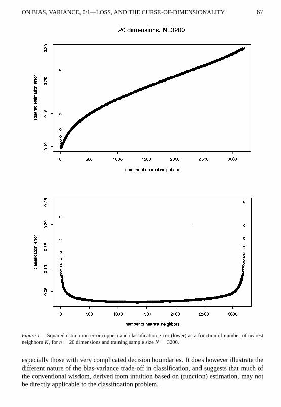
An important aspect contributing to the successful resistance of classification error to thecurse-of-dimensionality is the choice of a good value for the number of nearest neighborsK . The discussion in Section 7 suggests that this should be typically larger for classificationthan for estimation error. This is verified in Table 1 for our simple example (9.5). Figure 1shows plots of the typical dependence of both squared estimation error (upper frame) andclassification error (lower frame) onK (heren = 20, N = 3200). One sees that choice ofnumber of nearest neighbors is less critical for classification error so long asK is neithertoo small nor too large (here 500≤ K ≤ 2000). However, it must be substantiallylarger than the optimal value for estimation error (Table 1) in order to obtain near optimalclassification performance. Quite often whenK -nearest neighbors are compared to otherclassification methods a small value (K = 1 or K = 5, for example) is used. The simpleexample examined here suggests that, at least in some situations, this may underestimatethe performance achievable with theK -nearest neighbor approach. This was dramaticallydemonstrated by Rosen et al. (1995), and noted by Henley and Hand (1996), in the contextof specific (real data) problems.

The example (9.4), (9.5) studied here is a very simple one intended to illustrate theconcepts involved. It was specifically designed to be highly susceptible to the effects of thecurse-of-dimensionality. It may well not be representative of many classification problems,




Figure 1. Squared estimation error (upper) and classification error (lower) as a function of number of nearestneighborsK , for n = 20 dimensions and training sample sizeN = 3200.

especially those with very complicated decision boundaries. It does however illustrate thedifferent nature of the bias-variance trade-off in classification, and suggests that much ofthe conventional wisdom, derived from intuition based on (function) estimation, may notbe directly applicable to the classification problem.



68 FRIEDMAN

Another potential limitation of the study presented here is that only dimensionalities upto n = 20 were considered. In many problems, especially those involving signals andimages, there may be hundreds or even thousands of input variables. However, in thecontext of nearest neighbor methods the number of inputs is not the relevant factor. Theimportant quantity is the (local)intrinsic dimensionality of the joint distribution of inputvalues as characterized by the number of its singular values that are not small. Especiallywhen there are many inputs there is usually a high degree of association among them sothat the corresponding intrinsic dimensionality is fairly moderate. In such cases the resultspresented here will likely be relevant.

10. Boundary bias

An important ingredient contributing to the success of both naive Bayes andK -nearestneighbor procedures is negative boundary bias (7.1). So long asb( f (x), E f (x)) < 0 theycan use decreasing variance to overcome its (increasing) effect on boundary error (6.5) toproduce accurate classification atx. It is the (over-smoothing) nature of the (large) biasinherent in these methods that leads to predominately negative boundary bias at most inputpoints x, and thereby good overall classification performance. Non-negative boundarybias on the other hand devastates classification performance. In this case the boundaryerror is greater than 1/2 and decreasing varianceincreasesthat error. At such pointsxthe classification procedure has no alternative but to try to reduce estimation bias (5.5) inan attempt to bring boundary bias down to a negative value. This generally involves anincrease in variance and the favorable trade-off produced by their multiplicative interactioneffect (6.5) is lost.

The devastating effect of positive boundary bias in the context ofK -nearest neighborprocedures is illustrated by a simple example. This example is the same as that used inSection 9 (9.4), (9.5) but with a modification to the prior probabilities (4.1). Here we takethem to be unequal, specificallyπ1 = 3π0, so that the value of the output mean (7.2) isy = 3/4. Table 3 shows the values of average squared estimation error (second column),classification error (fourth column), along with their respective optimal number of nearestneighborsK (columns 3 and 5) as a function of sample sizeN (first column), atn = 20

Table 3. Error rates and optimalK as a function of sample sizeN for n = 20 withπ1 = 3π0.

N Est.2 Ke Class Kc Class(t = −1/4) Kc(t = −1/4)

100 .136 11 .195 5 .154 44

200 .125 11 .176 5 .110 96

400 .116 10 .164 5 .081 192

800 .109 14 .154 7 .060 372

1600 .100 15 .141 7 .043 772

3200 .092 17 .129 7 .029 1488

6400 .086 13 .118 7 .024 3292

12800 .078 14 .105 9 .016 4400




dimensions. For squared estimation error one sees similar results to that shown in Table 1for equal priors (π0 = π1). Error is large and decreases slowly with increasingN. Forclassification error however one sees a quite different result for unequal priors (π1 = 3π0).Classification error is here much larger than for equal priors and decreases very slowlywith increasingN at a rate similar to that for squared estimation error. The number ofnearest neighbors that minimize classification error is also very different for unequal priors;they are even smaller than those for squared estimation error and increase very slowlywith increasingN. For unequal priors (y 6= 1/2) classification error is suffering from thecurse-of-dimensionality in the same way as squared estimation error.

It is easy to see that the problem withK -nearest neighbors in this setting is positive bound-ary bias over much of the input space. The over-smoothed nature of the estimates causesthem to be shrunk towards the output meany (7.3) and in this casey is not equal to the clas-sification threshold (2.6), here 1/2. The boundary bias is non-negativeb( f (x), E f (x)) ≥ 0at all input pointsx for which x1 < 1/2 ( f (x) = 0) and 1/3 or more of the volume of theK -nearest neighborhood overlaps the class one regionx1 ≥ 1/2 (E f (x) ≥ 1/2). As thedimensionn increases the average radius of the regions (9.2), (9.3) increases (for fixedK )so that the portion of the input space with positive boundary bias also increases. The onlyway to mitigate this effect is to reduce the value ofK and thereby average region radius.For increasingn this strategy becomes less effective owing to the curse-of-dimensionality;average radius varies as thenth root ofK . At high dimensions there is considerable positiveboundary bias even forK = 1. Therefore, one sees slow decrease for average classificationerror with increasingN, typical of that associated with the curse-of-dimensionality.

For this particular example there is a simple remedy for this problem. One can simplyapply the procedure as if the prior probabilities were equal, even though there are three timesas many class ones as class zeros in both the training data and future data to be classified.This involves weighting each class zero training observation with three times the mass ofeach class one in the average leading to the computation off (x) (9.1). This simple trickcausesy = 1/2 (7.2) and thereby produces negative boundary bias everywhere in the inputspace for this problem. Applying such a weighting scheme is equivalent to modifying theestimatef (x) by the transformation

f (x) = f (x)+ t (10.1)

before inserting it into the output estimate (2.6) (heret = −1/4).The sixth column of Table 3 shows the corresponding classification error using the “bias

adjustment” (10.1) witht = −1/4, and the seventh column its corresponding optimalnumber of nearest neighbors. Applying the bias adjustmentt = −1/4 (10.1) causesthe boundary bias associated withf (x) to be everywhere negative and allows decreasingvariance (increasingK ) to maximally exploit their interaction effect (6.5) to dramaticallyreduce classification error.

The bias adjustment (10.1) changes both estimation (5.5) and boundary (7.1) bias every-where in the input space. The optimal value oft for estimation error iste = avex f (x) −avex f (x). Since these two averages tend to have similar values for most estimation proce-dures (especially those that over-smooth) there is seldom much to be gained by employing(10.1). In the case of boundary bias (7.1) the modification (10.1) decreases its value over



70 FRIEDMAN

half of the input space (x1 < 1/2) and increases it by the same amount at each pointxin the other half (x1 ≥ 1/2). Therefore average boundary bias is (substantially) increasedsince the (pooled) distribution of the input values places three times as much mass in thelatter half space (x1 ≥ 1/2). However the interaction between variance and boundary biasoccurs separately at each individual pointx, and the choicet = −1/4 (10.1) here providesthe right balance so that the boundary bias is negative at allx.

In this example a good bias adjustment valuet (10.1) could be determined since the truetarget function (9.5) and priors (π1 = 3π0) were known. This is seldom the case in practice.Even when they are known however a good choice may not be obvious. Consider the case

p0(x) = (4/3) · 1(x1 < 3/4), p1(x) = 4 · 1(x1 ≥ 3/4) (10.2)

with equal prior probabilities (π0 = π1), again on the hypercubex ∈ [0, 1]n. The targetprobability function (3.2) is

f (x) = 1(x1 ≥ 3/4). (10.3)

Here the response mean (7.2) isy = 1/2 but there is positive boundary bias over much ofthe input space, caused by the higher density of class ones near the decision boundary.

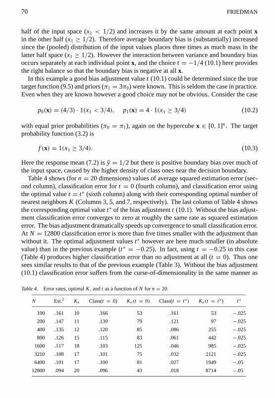
Table 4 shows (forn = 20 dimensions) values of average squared estimation error (sec-ond column), classification error fort = 0 (fourth column), and classification error usingthe optimal valuet = t∗ (sixth column) along with their corresponding optimal number ofnearest neighborsK (Columns 3, 5, and 7, respectively). The last column of Table 4 showsthe corresponding optimal valuet∗ of the bias adjustmentt (10.1). Without the bias adjust-ment classification error converges to zero at roughly the same rate as squared estimationerror. The bias adjustment dramatically speeds up convergence to small classification error.At N = 12800 classification error is more than five times smaller with the adjustment thanwithout it. The optimal adjustment valuest∗ however are here much smaller (in absolutevalue) than in the previous example (t∗ = −0.25). In fact, usingt = −0.25 in this case(Table 4) produces higher classification error than no adjustment at all (t = 0). Thus onesees similar results to that of the previous example (Table 3). Without the bias adjustment(10.1) classification error suffers from the curse-of-dimensionality in the same manner as

Table 4. Error rates, optimalK , andt as a function ofN for n = 20.

N Est.2 Ke Class(t = 0) Kc(t = 0) Class(t = t∗) Kc(t = t∗) t∗

100 .161 10 .166 53 .161 53 −.025

200 .147 11 .139 79 .121 97 −.025

400 .135 12 .120 85 .086 255 −.025

800 .126 15 .115 83 .061 442 −.025

1600 .117 18 .103 125 .046 985 −.025

3210 .108 17 .101 75 .032 2121 −.025

6400 .101 17 .100 81 .027 1949 −.05

12800 .094 20 .096 43 .018 8714 −.05




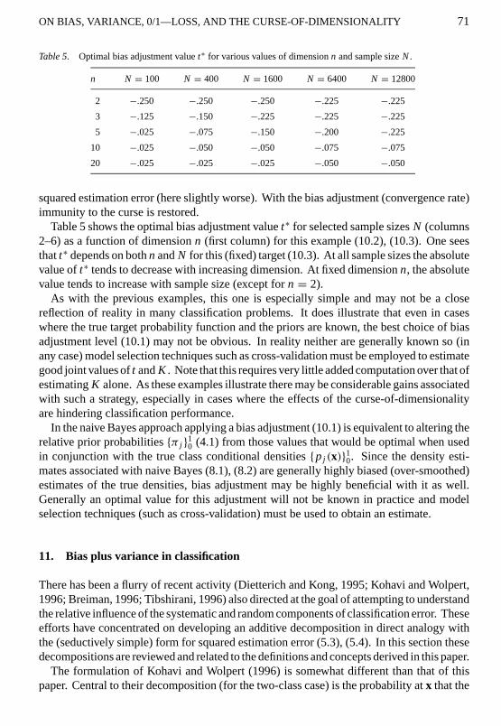
Table 5. Optimal bias adjustment valuet∗ for various values of dimensionn and sample sizeN.

n N = 100 N = 400 N = 1600 N = 6400 N = 12800

2 −.250 −.250 −.250 −.225 −.225

3 −.125 −.150 −.225 −.225 −.225

5 −.025 −.075 −.150 −.200 −.225

10 −.025 −.050 −.050 −.075 −.075

20 −.025 −.025 −.025 −.050 −.050

squared estimation error (here slightly worse). With the bias adjustment (convergence rate)immunity to the curse is restored.

Table 5 shows the optimal bias adjustment valuet∗ for selected sample sizesN (columns2–6) as a function of dimensionn (first column) for this example (10.2), (10.3). One seesthatt∗ depends on bothn andN for this (fixed) target (10.3). At all sample sizes the absolutevalue oft∗ tends to decrease with increasing dimension. At fixed dimensionn, the absolutevalue tends to increase with sample size (except forn = 2).

As with the previous examples, this one is especially simple and may not be a closereflection of reality in many classification problems. It does illustrate that even in caseswhere the true target probability function and the priors are known, the best choice of biasadjustment level (10.1) may not be obvious. In reality neither are generally known so (inany case) model selection techniques such as cross-validation must be employed to estimategood joint values oft andK . Note that this requires very little added computation over that ofestimatingK alone. As these examples illustrate there may be considerable gains associatedwith such a strategy, especially in cases where the effects of the curse-of-dimensionalityare hindering classification performance.

In the naive Bayes approach applying a bias adjustment (10.1) is equivalent to altering therelative prior probabilities{π j }10 (4.1) from those values that would be optimal when usedin conjunction with the true class conditional densities{pj (x)}10. Since the density esti-mates associated with naive Bayes (8.1), (8.2) are generally highly biased (over-smoothed)estimates of the true densities, bias adjustment may be highly beneficial with it as well.Generally an optimal value for this adjustment will not be known in practice and modelselection techniques (such as cross-validation) must be used to obtain an estimate.

11. Bias plus variance in classification

There has been a flurry of recent activity (Dietterich and Kong, 1995; Kohavi and Wolpert,1996; Breiman, 1996; Tibshirani, 1996) also directed at the goal of attempting to understandthe relative influence of the systematic and random components of classification error. Theseefforts have concentrated on developing an additive decomposition in direct analogy withthe (seductively simple) form for squared estimation error (5.3), (5.4). In this section thesedecompositions are reviewed and related to the definitions and concepts derived in this paper.

The formulation of Kohavi and Wolpert (1996) is somewhat different than that of thispaper. Central to their decomposition (for the two-class case) is the probability atx that the



72 FRIEDMAN

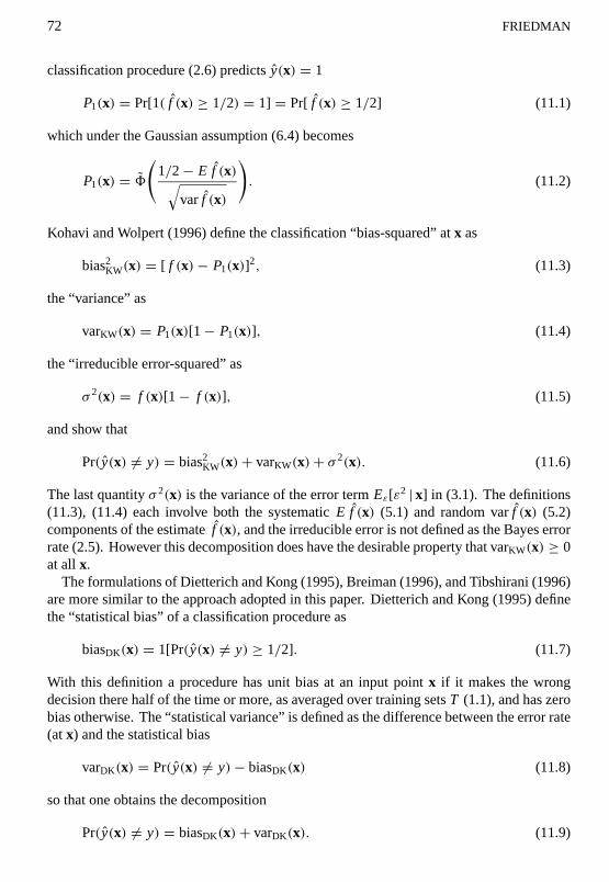
classification procedure (2.6) predictsy(x) = 1

P1(x) = Pr[1( f (x) ≥ 1/2) = 1] = Pr[ f (x) ≥ 1/2] (11.1)

which under the Gaussian assumption (6.4) becomes

P1(x) = 8(

1/2− E f (x)√var f (x)

). (11.2)

Kohavi and Wolpert (1996) define the classification “bias-squared” atx as

bias2KW(x) = [ f (x)− P1(x)]2, (11.3)

the “variance” as

varKW(x) = P1(x)[1− P1(x)], (11.4)

the “irreducible error-squared” as

σ 2(x) = f (x)[1− f (x)], (11.5)

and show that

Pr(y(x) 6= y) = bias2KW(x)+ varKW(x)+ σ 2(x). (11.6)

The last quantityσ 2(x) is the variance of the error termEε[ε2 | x] in (3.1). The definitions(11.3), (11.4) each involve both the systematicE f (x) (5.1) and random varf (x) (5.2)components of the estimatef (x), and the irreducible error is not defined as the Bayes errorrate (2.5). However this decomposition does have the desirable property that varKW(x) ≥ 0at allx.

The formulations of Dietterich and Kong (1995), Breiman (1996), and Tibshirani (1996)are more similar to the approach adopted in this paper. Dietterich and Kong (1995) definethe “statistical bias” of a classification procedure as

biasDK(x) = 1[Pr(y(x) 6= y) ≥ 1/2]. (11.7)

With this definition a procedure has unit bias at an input pointx if it makes the wrongdecision there half of the time or more, as averaged over training setsT (1.1), and has zerobias otherwise. The “statistical variance” is defined as the difference between the error rate(atx) and the statistical bias

varDK(x) = Pr(y(x) 6= y)− biasDK(x) (11.8)

so that one obtains the decomposition

Pr(y(x) 6= y) = biasDK(x)+ varDK(x). (11.9)




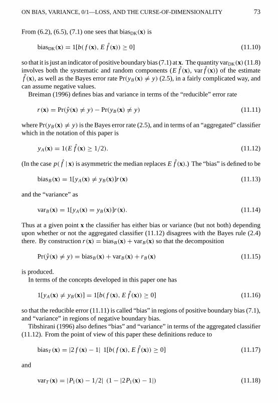
From (6.2), (6.5), (7.1) one sees that biasDK(x) is

biasDK(x) = 1[b( f (x), E f (x)) ≥ 0] (11.10)

so that it is just an indicator of positive boundary bias (7.1) atx. The quantity varDK(x) (11.8)involves both the systematic and random components (E f (x), var f (x)) of the estimatef (x), as well as the Bayes error rate Pr(yB(x) 6= y) (2.5), in a fairly complicated way, andcan assume negative values.

Breiman (1996) defines bias and variance in terms of the “reducible” error rate

r (x) = Pr(y(x) 6= y)− Pr(yB(x) 6= y) (11.11)

where Pr(yB(x) 6= y) is the Bayes error rate (2.5), and in terms of an “aggregated” classifierwhich in the notation of this paper is

yA(x) = 1(E f (x) ≥ 1/2). (11.12)

(In the casep( f | x) is asymmetric the median replacesE f (x).) The “bias” is defined to be

biasB(x) = 1[yA(x) 6= yB(x)]r (x) (11.13)

and the “variance” as

varB(x) = 1[yA(x) = yB(x)]r (x). (11.14)

Thus at a given pointx the classifier has either bias or variance (but not both) dependingupon whether or not the aggregated classifier (11.12) disagrees with the Bayes rule (2.4)there. By constructionr (x) = biasB(x)+ varB(x) so that the decomposition

Pr(y(x) 6= y) = biasB(x)+ varB(x)+ r B(x) (11.15)

is produced.In terms of the concepts developed in this paper one has

1[yA(x) 6= yB(x)] = 1[b( f (x), E f (x)) ≥ 0] (11.16)

so that the reducible error (11.11) is called “bias” in regions of positive boundary bias (7.1),and “variance” in regions of negative boundary bias.

Tibshirani (1996) also defines “bias” and “variance” in terms of the aggregated classifier(11.12). From the point of view of this paper these definitions reduce to

biasT (x) = |2 f (x)− 1| 1[b( f (x), E f (x)) ≥ 0] (11.17)

and

varT (x) = |P1(x)− 1/2| (1− |2P1(x)− 1|) (11.18)



74 FRIEDMAN

whereP1(x) (11.1) is the probability that the classifier (2.6) predictsy(x) = 1 atx. Thisdefinition of variance has a similar flavor to that of Kohavi and Wolpert (1996) (11.4);it has zero value whenP1(x) assumes its extreme values (0, 1) and is non-negative overthe entire range. However varT (x) (11.18) achieves its maximum value atP1(x) = 1/4and P1(x) = 3/4 and has the value zero atP1(x) = 1/2 where varKW(x) (11.4) takes onits maximum value. Using the definitions (11.17), (11.18) does not lead to an additivedecomposition of classification error in a form similar to that of (11.6), (11.9), or (11.15).

All of these additive decompositions are quite useful in providing insight into the natureof classification error. The bias definitions (11.10), (11.13), (11.16), and (11.17) all suggest(from different perspectives) the importance of the concept of boundary bias (7.1) developedin this paper. All emphasize the contribution of variability to the error rate of a classifier.This latter contribution especially (as noted by the authors) has often been overlooked inthe development of machine learning procedures. To the extent that the development inthis paper makes an additional contribution, it is that for classification error (unlike squaredestimation error) the systematic and random componentsinteract in a multiplicative andhighly nonlinear way, and this interaction effect can sometimes be exploited to reduce error.

12. “Aggregated” classifiers

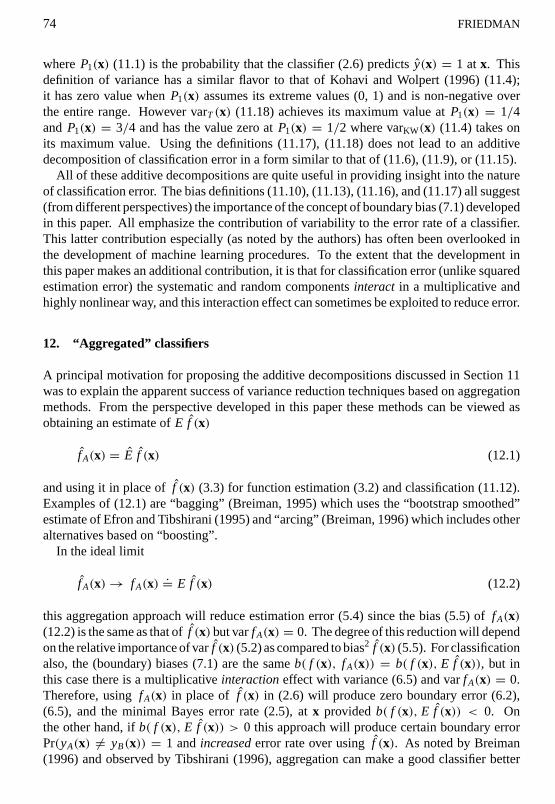
A principal motivation for proposing the additive decompositions discussed in Section 11was to explain the apparent success of variance reduction techniques based on aggregationmethods. From the perspective developed in this paper these methods can be viewed asobtaining an estimate ofE f (x)

f A(x) = E f (x) (12.1)

and using it in place off (x) (3.3) for function estimation (3.2) and classification (11.12).Examples of (12.1) are “bagging” (Breiman, 1995) which uses the “bootstrap smoothed”estimate of Efron and Tibshirani (1995) and “arcing” (Breiman, 1996) which includes otheralternatives based on “boosting”.

In the ideal limit

f A(x)→ fA(x).= E f (x) (12.2)

this aggregation approach will reduce estimation error (5.4) since the bias (5.5) offA(x)(12.2) is the same as that off (x) but varfA(x) = 0. The degree of this reduction will dependon the relative importance of varf (x) (5.2) as compared to bias2 f (x) (5.5). For classificationalso, the (boundary) biases (7.1) are the sameb( f (x), fA(x)) = b( f (x), E f (x)), but inthis case there is a multiplicativeinteractioneffect with variance (6.5) and varfA(x) = 0.Therefore, usingfA(x) in place of f (x) in (2.6) will produce zero boundary error (6.2),(6.5), and the minimal Bayes error rate (2.5), atx providedb( f (x), E f (x)) < 0. Onthe other hand, ifb( f (x), E f (x)) > 0 this approach will produce certain boundary errorPr(yA(x) 6= yB(x)) = 1 andincreasederror rate over usingf (x). As noted by Breiman(1996) and observed by Tibshirani (1996), aggregation can make a good classifier better




but can make a bad classifier worse. Clearly, this effect occurs separately at each individualprediction pointx, so success of aggregation for classification depends on the relative sizeof the portion of the input space with negative boundary bias.

As discussed in Section 10 the success of variance reduction techniques for classificationcan be enhanced by the use of a bias adjustment (10.1) tof (x). This is a consequence of the(boundary) bias-variance multiplicative interaction effect at eachx. For the same reason itseems likely that such an adjustment

f A(x) = f A(x)+ t (12.3)

will be beneficial in the context of aggregated classification as well. Bias adjustment (10.1),(12.3) can (sometimes dramatically) reduce the proportion of the input space with positiveboundary bias. As with other methods of variance reduction a good adjustment valuet isnot likely to be known in any particular situation, and therefore it will have to be estimatedthrough some model selection technique such as cross-validation.

13. Limitations and future work

The most serious limitation of the work presented here is the restriction to the two-classproblem. Intuition suggests that many of the concepts developed in this context may haveanalogs in theL ≥ 3 class case, but the detailed development will be more complicated.In particular, there will likely be analogs to the notion of boundary bias and its interactionwith the variances of the estimates of theL target probability functions{ fl (x)}L1 . Also theconcept of bias adjustment(s) may also be helpful in the multi-class problem. This is leftfor future work.

Another limitation is the use of the Gaussian approximation (6.4). This is clearly not cru-cial to the qualitative results obtained. For example, the distribution ofK -nearest neighborestimates is not strictly Gaussian but, as seen in Section 9, its behavior closely follows thatsuggested by (6.5). As noted, the median ofp( f | x) should replace the meanE f (x) in thedefinition of boundary bias (7.1) in the case of asymmetry, and an appropriate measure ofits spread (variability off (x)) would substitute for

√var f (x) in deriving a boundary error

analog to (6.5). Clearly, these two quantities would strongly interact in whatever detailedform emerged from the derivation.

The illustrative examples presented were intensionally chosen to be quite simple so thatone could easily understand the geometry of the decision boundaries, and thus the natureof the boundary bias (7.1) associated with the classification methods studied here. Actualdecision boundaries for specific problems encountered in practice may of course be quitedifferent, as could the nature of the boundary bias associated with other classificationmethods. Thus the gains associated with bias adjustment (10.1) may not be the same inother situations. All of this is problem dependent and can only be determined throughexperimentation in each specific case.

The goal of the work presented here is to illustrate that classification error responds toerror in the target probability estimates in a much different (and perhaps less intuitive)way than squared estimation error. This helps explain why improvements to the latter do



76 FRIEDMAN

not necessarily lead to improved classification performance, and why simple methods suchas naive Bayes,K -nearest neighbors, and others remain competitive, even though theyusually provide very poor estimates of the true underlying probabilities. Good probabilityestimates are not necessary for good classification; similarly, low classification error doesnot imply that the corresponding class probabilities are being estimated (even remotely)accurately. An understanding of these issues may help improve the chance of success offuture methodological developments.

Acknowledgments

Enlightening discussions with Trevor Hastie, Art Owen, and David Rosen are gratefullyacknowledged. Work supported in part by the Department of Energy under contract num-ber DE-AC03-76SF00515 and by the National Science Foundation under grant numberDMS-9403804.

References

Bellman, R.E. 1961. Adaptive Control Processes. Princeton University Press.Breiman, L. 1995. Bagging predictors. Dept. of Statistics, University of California, Berkeley, Technical Report.Breiman, L. 1996. Bias, variance, and arcing classifiers. Dept. of Statistics, University of California, Technical

Report (revised).Breiman, L., Friedman, J.H., Olshen, R.A., and Stone, C.J. 1984. Classification and Regression Trees. Wadsworth.Chow, W.S. and Chen, Y.C. 1992. A new fast algorithm for effective training of neural classifiers. Pattern Recog-

nition, 25:423–429.Dietterich, T.G. and Kong, E.B. 1995. Machine learning bias, statistical bias, and statistical variance of decision

tree algorithms. Dept. of Computer Science, Oregon State University Technical Report.Efron, B. and Tibshirani, R. 1995. Cross-validation and the bootstrap: Estimating the error rate of a prediction

rule. Dept. of Statistics, Stanford University Technical Report.Fix, E. and Hodges, J.L. 1951. Discriminatory analysis—nonparametric discrimination: Consistency properties.

Randolf Field Texas: U.S. Airforce School of Aviation Medicine Technical Report No. 4.Friedman, J.H. 1985. Classification and multiple response regression through projection pursuit. Dept. of Statistics,

Stanford University Technical Report LCS012.Geman, S., Bienenstock, E., and Doursat, R. 1992. Neural networks and the bias/variance dilemma. Neural Comp.,

4:1–48.Good, I.J. 1965. The Estimation of Probabilities: An Essay on Modern Bayesian Methods. M.I.T. Press.Hand, D.J. 1982. Kernel discriminant analysis. Chichester: Research Studies Press.Heckerman, D., Geiger, D., and Chickering, D. 1994. Learning Bayesian networks: the combination of knowledge

and statistical data. In Proceedings of the Tenth Conference on Uncertainty in Artificial Intelligence, pp. 293–301, AAAI Press and M.I.T. Press.

Henley, W.E. and Hand, D.J. 1996. Ak-nearest neighbour classifier for assessing consumer credit risk. TheStatistician, 45:77–95.

Holte, R.C. 1993. Very simple classification rules perform well on most commonly used data sets. MachineLearning, 11:63–90.

Kohavi, R. and Wolpert, D.H. 1996. Bias plus variance decomposition for zero-one loss functions. Dept. ofComputer Science, Stanford University Technical Report.

Kohonen, T. 1990. The self-organizing map. Proceedings of the IEEE, 78:1464–1480.Langley, P., Iba, W., and Thompson, K. 1992. An analysis of Bayesian classifiers. In Proceedings of the Tenth

National Conference on Artificial Intelligence, pp. 223–228, AAAI Press and M.I.T. Press.Lippmann, R. 1989. Pattern classification using neural networks. IEEE Communications Magazine, 11:47–64.




McLachlan, G.J. 1992. Discriminant Analysis and Statistical Pattern Recognition. Wiley.Quinlan, J.R. 1993. C4.5: Programs for Machine Learning. Morgan Kaufmann.Rosen, D.B., Burke, H.B., and Goodman, P.H. 1995. Local learning methods in high dimension: Beating the

bias-variance dilemma via recalibration. Workshop Machines That Learn—Neural Networks for Computing,Snowbird Utah.

Tibshirani, R. 1996. Bias, variance and prediction error for classification rules. Dept. of Statistics, University ofToronto Technical Report.

Titterington, D.M., Murray, G.D., Murray, L.S., Spiegelhalter, D.J., Skene, A.M., Habbema, J.D.F., and Gelpke,G.J. 1981. Comparison of discrimination techniques applied to a complex data set of head injured patients.J. Roy. Statist. Soc. A, 144:145–175.

Jerome H. Friedman received the Ph.D. degree in Physics from the University of California, Berkeley. He ispresently Professor of Statistics at Stanford University. He has been engaged in research on techniques for theanalysis of large complex data sets for over 20 years.

Documents

On Bias, Variance, 0/1—Loss, and the Curse-of …sushil/class/ml/papers/local/curseDim.pdf · and the Curse-of-Dimensionality ... “training” sample T Dfxi;yigN 1 ... wisdom