International Journal of Bifurcation and Chaos, Vol. 8, No. 4 (1998) 685–699c© World Scientific Publishing Company

ON BIFURCATIONS LEADING TO CHAOSIN CHUA’S CIRCUIT

V. V. BYKOV∗

Institute for Applied Mathematics & Cybernetics,Ul’janova st. 10, 603005, Nizhny Novgorod, Russia

Received July 15, 1996; Revised February 5, 1997

Bifurcations and the structure of limit sets are studied for a three-dimensional Chua’s circuitsystem with a cubic nonlinearity. On the base of both computer simulations and theoreticalresults a model map is proposed which allows one to follow the evolution in the phase space froma simple (Morse-Smale) structure to chaos. It is established that the appearance of a complex,multistructural set of double-scroll type is stimulated by the presence of a heteroclinic orbitof intersection of the unstable manifold of a saddle periodic orbit and unstable manifold of anequilibrium state of saddle-focus type.

1. Introduction

Nowadays, there exists a specific interest in thestudy of dynamical systems with chaotic behav-ior. The stimulating factor is that the phenomenonof dynamical chaos is typical in some sense and itis found in many applications. Usually, there ap-pear difficulties with the answer on the followingquestions: which limit sets the stochastic behavioris connected with and what is the mechanism oftransition from regular oscillations to the stochas-tic regime? Rigorously, the mathematical image ofstochastic oscillations may be an attractive tran-sitive limit set consisting of unstable orbits, thatis a strange attractor. The well-known example isLorenz attractor [Afraimovich et al., 1977, 1983].

However, very often the appearance of chaosis connected with more complicated mathematicalobject: with a limit set containing nontrivial hy-perbolic sets as well as stable periodic orbits (thelatter may be invisible due to small absorbing do-mains and large periods). Such limit sets maygenerate stochastic oscillations because of the pres-ence of perturbations stimulated by the inevitable

presence of noise in experiments and by round-offerrors in computer modeling. These limit sets areknown as quasiattractors [Afraimovich & Shil’nikov,1983].

A typical example of a quasiattractor is theso-called Rossler attractor arising after a period-doubling cascade. Another example is the spiralattractor which, somehow, is a union of the Rosslerattractor and the unstable limit set near a ho-moclinic loop of a saddle-focus [Shil’nikov, 1991].Also, if two spiral quasiattractors unite includingthe saddle-focus together with its invariant unstablemanifold, then a more complicated set arise whichis called double-scroll [Chua et al., 1986].

The quasiattractors listed above are not ab-stract mathematical objects but they correspond toreal processes visible in experiments as well as incomputer simulations with, for instance, the well-known Chua’s circuit (Fig. 1) [Madan, 1993]. Thestudy of this circuit was mainly carried out forthe case of piecewise linear approximation of thenonlinear element [Chua et al., 1986, Chua & Lin,1991; George, 1986]. Note that the interest to the

∗E-mail: bykov@focus.nnov.su

685

686 V. V. Bykov

Fig. 1. Circuit scheme for Chua’s circuit.

piecewise linear representation is, apparently, con-nected not with the technical aspect of the problembut with the idea of the applicability of analyticalmethods for this case. It happened, nevertheless,that the complexity of the analytical expressionsarising here is too high, their immediate analysis isquite difficult and cannot actually be done withoutuse of numerical methods. In fact, the direct com-puter simulations of the differential equations hasappeared to be more effective. Note also that thepiecewise linear approximation does not allow oneto use the full capacity of the methods and results ofthe bifurcation theory developed mostly for smoothdynamical systems. All this were the reasons whythe characteristic of the nonlinear element was mod-eled in [Freire et al., 1993; Khibnic et al., 1993] bya cubic polynomial which retains the main geomet-rical features of the piecewise linear approximation.This choice provided the possibility of studyinglocal bifurcations by analytical methods and, then,by numerical simulation, to show the presence ofglobal bifurcations, in particular, those which indi-cate chaotic dynamics.

The scope of the present paper is to study themain bifurcations and the structure of limit sets forthe following three-dimensional system.

x = β(g(y − x)− h(x)), y = g(x− y) + z ,

z = −y(1)

where β, g, α are positive parameters describingthe aforementioned electronic circuit for the cubicalh(x) = αx(x2 − 1) approximation of the nonlinearelement. The parameters β and g are connectedwith the physical parameters of the circuit as fol-lows: β = C1/C2, g = G/ωC1 where ω = 1/

√LC2.

In spite of intensive theoretical and experimen-tal studies, the question of principal bifurcationswith which the birth of the double-scroll quasi-attractor in the model is connected is not quiteclear till now. The usual explanation based on theShil’nikov theorem [1970] concerning the bifurca-tion of saddle-focus homoclinic loops is not com-pletely satisfactory here because the hyperbolic setlying near the loop is not attractive. Therefore, theestablishing of the presence of such loops is not suffi-cient for the existence of chaotic attractors. It willbe shown, for instance, that for system (1) thereexists a region in the parameter space where the bi-furcational set corresponding to a single-round ho-moclinic loop of a saddle-focus lies, and Shil’nikovconditions are satisfied, but there is no chaotic at-tractor and most of orbits tend to a stable limitcycle.

In the present paper it is established that theappearance of the double-scroll is connected withthe presence of heteroclinic orbits of intersection oftwo-dimensional invariant manifolds of the saddle-focus and a saddle periodic orbit. In one case this isone of periodic orbits lying in the Rossler attractor;it may also be a symmetric periodic orbit arisingthrough a condensation of orbits. This assertion isbased on the study of a model map by the use ofwhich the birth and the structure of an attractivelimit set can be described which is the intersectionof the double-scroll with a cross-section.

Note that the double scroll contains the saddle-focus which may have homoclinic loops; also, thedouble-scroll may contain structurally unstable ho-moclinic orbits of saddle periodic orbits. By virtueof [Ovsyannikov & Shil’nikov, 1987; Gavrilov &Shilnikov, 1973; Newhouse, 1979], this impliesthat stable periodic orbits may appear in thedouble-scroll and it is, therefore, a quasiattractor[Shil’nikov, 1994]. This is the reason why the bifur-cational set which corresponds to the birth of thedouble-scroll and which is a smooth curve containsa Cantor set of points of intersection with bifurca-tional curves corresponding to the situation wherethe one-dimensional separatrix of the saddle-focusbelongs to the stable manifold of some nontrivialhyperbolic set. In the adjoint intervals the sepa-ratrix, apparently tends to one of the stable peri-odic orbits. A component of the bifurcational curveof the birth of the double-scroll can also be foundwhich corresponds to the tangency of the stable andunstable manifolds of the hyperbolic set.

On Bifurcations Leading to Chaos in Chua’s Circuit 687

2. The Scenario of Transitionto Chaos

2.1. Local bifurcations

Consider the sequence of the basic bifurcationswith which the appearance of complex limit setsis connected. We begin with the study of equilib-rium states. When g > α there exists only oneequilibrium state O in the origin. When g < αthere also exist two symmetric equilibrium statesO1, O2 with the coordinates x∗1,2 = ±

√1− g/a,

y∗ = 0, z∗1,2 = ∓√

1− g/α. In this region of theparameter space O is unstable: it is a saddle or asaddle-focus with one positive characteristic expo-nent. The one-dimensional separatrices of O willbe denoted as Pi, i = 1, 2, and the two-dimensionalstable manifold of O will be denoted as W s(O).

On the line g = α the characteristic equation of0 has one zero root for β 6= 1/α2 and it has two zeroroots at β = 1/α2. We denote this point on the pa-rameter plane (β, g/α) as TH (Takens–Harozov).The bifurcations in the neighborhood of this pointare known [Harozov, 1979] to be determined by the

following normal form on the center manifold:

x = y, y = εx+ µy + ax3 + γx2y .

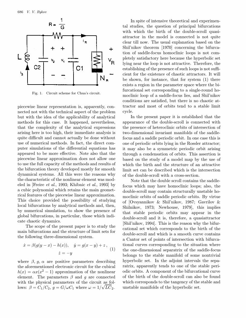
In our case, for system (1) we have a =−1/α2, γ = 3(α2 − 1)/α3, and the bifurcation dia-gram corresponding to α < 1 has the form shownin Fig. 3 [Harozov, 1979 & Arnold, 1982]. Note thepresence of the curve SL which corresponds to a ho-moclinic loop of the saddle O. In a sufficiently small

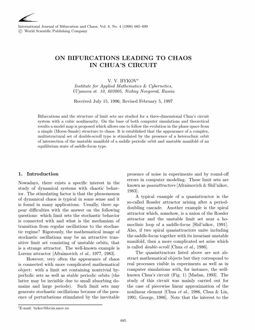
Fig. 2. The double-scroll quasiattractor.

Fig. 3. The local bifurcation diagram on the β–g/a plane at a = 0.2. Three codimension-2 bifurcation points (TH, Takens–Harozov; DH0, a degenerate Andronov–Hopf bifurcation of the origin; B, Bel’jakov point — a homoclinic loop to a saddle-focuswith the saddle index ν equal to 1) and several codimension-1 bifurcation curves (PI, pitchfork of equilibria; H0, Andronov–Hopf of the origin; H1, Andronov–Hopf of nontrivial equilibria; SN and sn, saddle-node bifurcation of periodic orbits;SL — homoclinic loop of the origin) are present.

688 V. V. Bykov

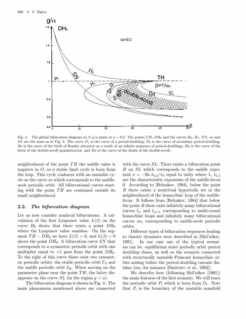
Fig. 4. The global bifurcation diagram on β–g/a plane at a = 0.2. The points TH, DH0 and the curves H0, H1, SN, sn andSL are the same as in Fig. 3. The curve D1 is the curve of a period-doubling, D2 is the curve of secondary period-doubling,Ra is the curve of the birth of Rossler attractor as a result of an infinite sequence of period-doublings, Ba is the curve of thebirth of the double-scroll quasiattractor, and Da is the curve of the death of the double-scroll.

neighborhood of the point TH the saddle value isnegative in O, so a stable limit cycle is born fromthe loop. This cycle coalesces with an unstable cy-cle on the curve sn which corresponds to the saddle-node periodic orbit. All bifurcational curves start-ing with the point TH are continued outside itssmall neighborhood.

2.2. The bifurcation diagram

Let us now consider nonlocal bifurcations. A cal-culation of the first Lyapunov value L(β) on thecurve H0 shows that there exists a point DH0

where the Lyapunov value vanishes. On the seg-ment TH −DH0 we have L(β) > 0, and L(β) < 0above the point DH0. A bifurcation curve SN thatcorresponds to a symmetric periodic orbit with onemultiplier equal to +1 goes from the point DH0.To the right of this curve there exist two symmet-ric periodic orbits: the stable periodic orbit Γ0 andthe saddle periodic orbit L0. When moving on theparameter plane near the point TH, the latter dis-appears on the curve SL (in the region g < α).

The bifurcation diagram is shown in Fig. 4. Themain phenomena mentioned above are connected

with the curve SL. There exists a bifurcation pointB on SL which corresponds to the saddle expo-nent ν = −Reλ1,2/λ3 equal to unity where λ, λ1,2

are the characteristic exponents of the saddle-focus0. According to [Belyakov, 1984], below the pointB there exists a nontrivial hyperbolic set in theneighborhood of the homoclinic loop of the saddle-focus. It follows from [Belyakov, 1984] that belowthe point B there exist infinitely many bifurcationalcurves lij and lij+1 corresponding to multi-roundhomoclinic loops and infinitely many bifurcationalcurves sni corresponding to saddle-node periodicorbits.

Different types of bifurcation sequences leadingto chaotic dynamics were described in [Shil’nikov,1991]. In our case one of the typical scenar-ios can be: equilibrium state–periodic orbit–perioddoubling–chaos, as well as the scenario connectedwith structurally unstable Poincare homoclinic or-bits arising before the period-doubling cascade fin-ishes (see, for instance [Dmitriev et al., 1992]).

We describe here (following Shil’nikov [1991])the main features of the first scenario. We will tracethe periodic orbit Pi which is born from Oi. Notethat Pi is the boundary of the unstable manifold

On Bifurcations Leading to Chaos in Chua’s Circuit 689

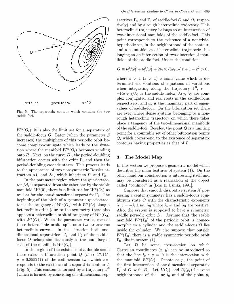
Fig. 5. The separatrix contour which contains the twosaddle-foci.

W u(Oi); it is also the limit set for a separatrix ofthe saddle-focus O. Later (when the parameter βincreases) the multipliers of this periodic orbit be-come complex-conjugate which leads to the situa-tion where the manifold W u(Oi) becomes windingonto Pi. Next, on the curve D1, the period-doublingbifurcation occurs with the orbit Γi and then theperiod-doubling cascade starts. This process leadsto the appearance of two nonsymmetric Rossler at-tractors M1 and M2 which inherit to P1 and P2.

In the parameter region where the quasiattrac-torMi is separated from the other one by the stablemanifold W s(0), there is a limit set for W u(Oi) aswell as for the one-dimensional separatrix Γi. Thebeginning of the birth of a symmetric quasiattrac-tor is the tangency of W u(O1) with W s(O) along aheteroclinic orbit (due to the symmetry there alsoappears a heteroclinic orbit of tangency of W u(O2)with W s(O)). When the parameter varies, each ofthese heteroclinic orbits split onto two transverseheteroclinic curves. In this situation both one-dimensional separatrices Γ1 and Γ2 of the saddle-focus O belong simultaneously to the boundary ofeach of the manifolds W u(Oi).

In the region of the existence of a double-scrollthere exists a bifurcation point Q (β ≈ 17.145,g ≈ 0.855247) of the codimension two which cor-responds to the existence of a separatrix contour L(Fig. 5). This contour is formed by a trajectory Γ0

(which is formed by coinciding one-dimensional sep-

aratrixes Γ0 and Γ1 of saddle-foci O and O1 respec-tively) and by a rough heteroclinic trajectory. Thisheteroclinic trajectory belongs to an intersection oftwo-dimensional manifolds of the saddle-foci. Thispoint corresponds to the existence of a nontrivialhyperbolic set, in the neighborhood of the contour,and a countable set of heteroclinic trajectories be-longing to an intersection of two-dimensional man-ifolds of the saddle-foci. Under the conditions

G ≡ ν21/ω

21 + ν2

2/ω22 + 2ν1ν2/(ω1ω2)ε+ 1− ε2 > 0 ,

where ε > 1 (ε > 1) is some value which is de-termined via solutions of equations in variationswhen integrating along the trajectory Γ0, ν =−Reλ1,2/λ3 is the saddle index, λ1,2, λ3 are com-plex conjugated and real roots in the saddle-focusrespectively, and ωi is the imaginary part of eigen-values of saddle-foci. On the bifurcation set thereare everywhere dense systems belonging to a non-rough heteroclinic trajectory on which there takesplace a tangency of the two-dimensional manifoldsof the saddle-foci. Besides, the point Q is a limitingpoint for a countable set of other bifurcation pointsQi which correspond to the existence of separatrixcontours having properties as that of L.

3. The Model Map

In this section we propose a geometric model whichdescribes the main features of system (1). On theother hand our construction is interesting itself andmay be considered as a realization of the objectcalled “confinor” in [Lozi & Ushiki, 1991].

Suppose that smooth dissipative system X pos-sessing a center symmetry has a saddle-focus equi-librium state O with the characteristic exponentsλ1,2 = −λ± iω, λ3 where λ, ω and λ3 are positive.Also, the system is supposed to have a symmetricsaddle periodic orbit L0. Assume that the stablemanifold W s(L0) of the periodic orbit is homeo-morphic to a cylinder and the saddle-focus O liesinside the cylinder. We also suppose that outsideW s(L0) there is a stable symmetric periodic orbitΓ0, like in system (1).

Let D be some cross-section on whichCartesian coordinates (x, y) can be introduced sothat the line l0 : y = 0 is the intersection withthe manifold W s(O). Denote as pi the point ofthe first intersection of one-dimensional separatrixΓi of O with D. Let U(l0) and Ui(pi) be someneighborhoods of the line l0 and of the point p1

690 V. V. Bykov

respectively and let U+(l0) (U−(l0)) be the com-ponent of U(l0) corresponding to the positive (re-spectively negative) values of y. According to[Gavrilov & Shilnikov, 1973; Shil’nikov, 1994], themap U+(l0) → U1(p1) defined by the orbits of thesystem is represented in the form

x = x∗ + b1 · x · yν cos(ω · ln(y) + θ1) + ψ1(x, y)

y = y∗ + b2 · x · yν sin(ω · ln(y) + θ2) + ψ2(x, y)

(2)

where ψi are smooth functions which tend, asy → 0, to zero along with their first derivative withrespect to y. An analogous formula is valid for themap U−(l0) → U2(p2). An extrapolation of theproperties of the local map defined by (2) leads tothe following construction which is in a good agree-ment with the results of computer simulation.

Consider two components D+ and D− intowhich the cross-section D is divided by theline l0; i.e. D = D+⋃D−⋃ l0. We have D+ =(x, y)||x| ≤ c, 0 < y ≤ h∗(x)|, D− = (x, y)||x| ≤c, −h(x) ≤ y < 0, where y = h∗(x) is a componentof the intersection of the stable manifold W s(L0)with D. The orbits of the system define the mapsT (µ)+ : D+ → D, T (µ)− : D− → D, and T (µ)+

and T (µ)− are written as

x = f+(x, y, µ), y = g+(x, y, µ)

and

x = f−(x, y, µ), y = g−(x, y, µ)

respectively; here, f+, f−, g+, g− ∈ Cr, and µ =(µ(1), µ(2)).1

The following properties are assumed for thesemaps.

(1) T+ and T− can be defined on l0 sothat limy→+0 T

+M(x, y) = (x∗, y∗), limy→−0

T−M(x, y) = (x∗∗,−y∗), where p1(x∗, y∗) andp2(x∗∗, −y∗) are the points of the first inter-section of one-dimensional separatrices of thesaddle-focus O with D. We suppose that Tdepends on µ in the following way: the firstcomponent of µ shifts the point P1 in verticaldirection and the second component of µ shiftsit in horizontal direction.

(2) Each of the regions D+, D− are represented asa union of an infinite number of regions S+

0 , S−0 ,S+i , S−i S

+i = (x, y)||x| ≤ c, ξ∗i+1 ≤ y < ξ∗i ,

S−i = (x, y)||x| ≤ c, −ξ∗i < y ≤ −ξ∗i+1,i = 1, . . . , where ξ∗0 = h∗(x), limi→∞ |ξ∗i | = 0.The map T+ or T− acts so that the image of anyvertical segment with one end-point on l0 hasthe form of a spiral winding at the point p1 orp2, respectively. The boundary γ±i : y = ξ∗i+1 of

two adjoining regions S±i, S±i+1 is chosen so that

∂y/∂y = 0 if and only if (x, y) ∈ γ±i , and T±γ±

is a segment of a curve of the form x = hi(y)where |dh/dy| < 1.

Introduce the following notations:

D1 = (x, y)| − c ≤ x ≤ −c/2, |y| < h(x) ,

D2 = (x, y)|c/2 ≤ x ≤ c, |y| < h(x) ,

D+i = D+

⋂Di, D

−i = D−

⋂DI ,

T ≡ T±|D±, (f±, g±) ≡ (f, g) ,

Si ≡ S±i , γi ≡ γ±iLet S+

0 (S−0 ) be that part of S+0 (S−0 ) on

which TS+0 ∈ D1 (TS−0 ∈ D2). Suppose that

the map T satisfies the following additionalconditions:

(3) TD1 ⊂ D, TD2 ⊂ D;(4) |∂x/∂x| < 1;(5) ri = %(Tγi, Tγi+1) > qξ∗i , q > 2, i > 1;(6) in Si there can be a set σi selected such that

the following inequality is fulfilled everywhereon σi:

‖gy‖ > 1 ,

1− ‖fx · g−1y ‖ < 2

√‖fy · g−1

y ‖ · ‖gx · g−1y ‖

(7) p1 ∈ S+0 , p2 ∈ S−0

Note that condition (2) is fulfilled near the linel0 (i.e. for the sets Si with i sufficiently large) byvirtue of (2). Conditions (3)–(5) are also auto-matically fulfilled near l0 if the saddle index ρ =−Reλ1,2/λ3 is less than unity in the saddle-focus.Moreover, in this case ri/ξ

∗i → ∞ as i → ∞; in

other words, q →∞ as i→∞.2

1The original double-scroll model map of the Chua attractor, see [Belykh & Chua, 1992].2The validity of such a model can be verified by computer simulations. It occurs that the contraction in horizontal directionis so strong that the images of the region x =

√1− g/a/2 under the action of the Poincare map have, in natural scale, the

form of one-dimensional curves [Figs. 6(b)–9(b) and 13(b)]

On Bifurcations Leading to Chaos in Chua’s Circuit 691

(a) (b)

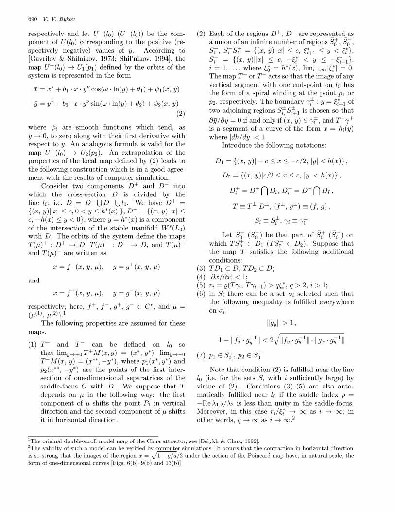
Fig. 6. The Poincare map on the semi-plane x =√

(1− g/a), y >√

(1− g/a)(β− 1/4)/2β for the parameter values lying tothe left of the bifurcation curve D1; (a) the theoretical model, (b) computer simulations.

(a) (b)

Fig. 7. As Fig. 6 with values of β and g/a lying to the right of the curve D1.

The fulfillment of condition (6) means that forthose parameter values for which there exist i andj such that the map σi → σj is defined, the opera-tor Tij : Hi(L)→ Hj(L) is contracting [Shashkov &

Shil’nikov, 1994; Afraimovich & Shil’nikov, 1973],where Hi(L) is the space of the curves y = ϕ(x) ly-ing in σi and satisfying the Lipschitz condition withsome Lipschitz constant L.

692 V. V. Bykov

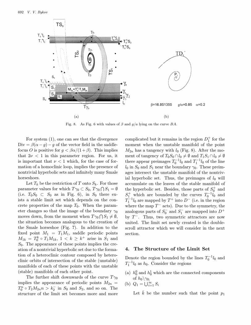
(a) (b)

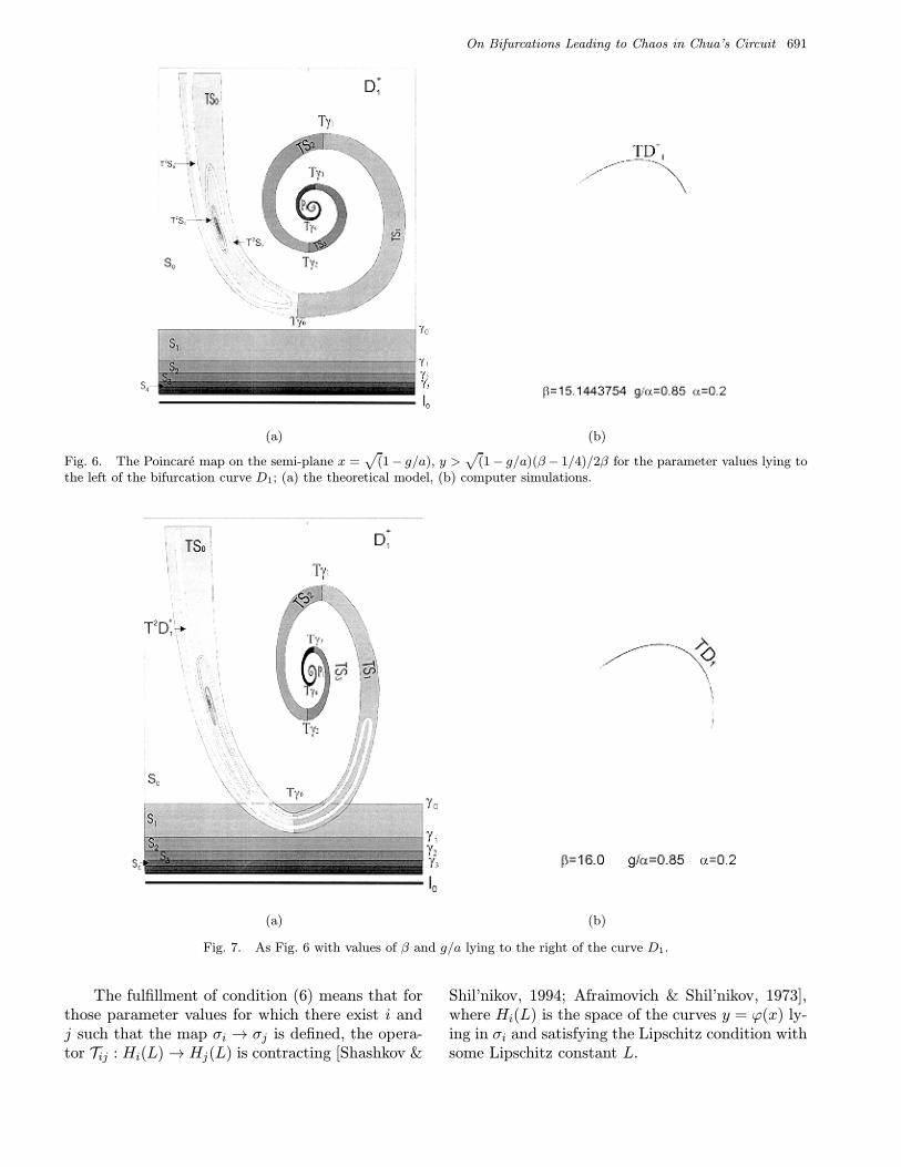
Fig. 8. As Fig. 6 with values of β and g/a lying on the curve BA.

For system (1), one can see that the divergenceDiv = β(α− g)− g of the vector field in the saddle-focus O is positive for g < βα/(1+β). This impliesthat 2ν < 1 in this parameter region. For us, itis important that ν < 1 which, for the case of for-mation of a homoclinic loop, implies the presence ofnontrivial hyperbolic sets and infinitely many Smalehorseshoes.

Let Tk be the restriction of T onto Sk. For thoseparameter values for which Tγ0 ⊂ S0, Tγ0

⋂S1 = ∅

(i.e. T0S0 ⊂ S0 as in Fig. 6), in S0 there ex-ists a stable limit set which depends on the con-crete properties of the map T0. When the param-eter changes so that the image of the boundary γ0

moves down, from the moment when Tγ0⋂S1 6= ∅,

the situation becomes analogous to the creation ofthe Smale horseshoe (Fig. 7). In addition to thefixed point M1 = T1M1, saddle periodic pointsM1k = T k0 T1M1k, 1 < k ≥ k+ arise in S1 andS0. The appearance of these points implies the cre-ation of a nontrivial hyperbolic set due to the forma-tion of a heteroclinic contour composed by hetero-clinic orbits of intersection of the stable (unstable)manifolds of each of these points with the unstable(stable) manifolds of each other point.

The further shift downwards of the curve Tγ0

implies the appearance of periodic points M2n =Tn0 T2M2nn > k−2 in S0 and S2, and so on. Thestructure of the limit set becomes more and more

complicated but it remains in the region D+1 for the

moment when the unstable manifold of the pointM2n has a tangency with l0 (Fig. 8). After the mo-ment of tangency of T0S0∩ l0 6= ∅ and T1S1∩ l0 6= ∅there appear preimages T−1

0 l0 and T−11 l0 of the line

l0 in S0 and S1 near the boundary γ0. These preim-ages intersect the unstable manifold of the nontriv-ial hyperbolic set. Thus, the preimages of l0 willaccumulate on the leaves of the stable manifold ofthe hyperbolic set. Besides, those parts of S+

0 andS+

1 which are bounded by the curves T−10 l0 and

T−11 l0 are mapped by T+ into D− (i.e. in the region

where the map T− acts). Due to the symmetry, theanalogous parts of S−0 and S−1 are mapped into D+

by T−. Thus, two symmetric attractors are nowunited. The limit set newly created is the double-scroll attractor which we will consider in the nextsection.

4. The Structure of the Limit Set

Denote the region bounded by the lines T−10 l0 and

T−11 l0 as h0. Consider the regions

(a) h00 and h1

0 which are the connected componentsof h0\γ0;

(b) Q1 =⋃∞i=1 Si

Let k be the number such that the point p1

On Bifurcations Leading to Chaos in Chua’s Circuit 693

(a)

(b)

Fig. 9. As Fig. 5 with values β, g/a lying to the right of the curve BA.

belongs to T−k0 (Q1⋃h0

0). Denote

k+1 = maxk|T−k0 (Q1

⋃h0

0) ∩ T1S1 6= ∅ ,

Tγ1 ∩ T−k0 (Q1 ∪ h00) = ∅

and

R1 = S1

∖h10

k+1⋃

k=1

(T−11 T−k0 (Q1

⋃h0

0))

.

694 V. V. Bykov

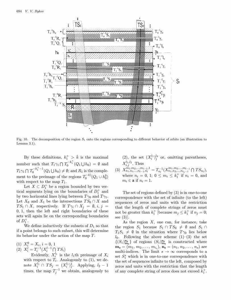
Fig. 10. The decomposition of the region S1 onto the regions corresponding to different behavior of orbits (an illustration toLemma 3.1).

By these definitions, k+1 > k is the maximal

number such that T1γ1⋂T−k+

10 (Q1

⋃h0) = ∅ and

T1γ1⋂T−k+

1 −10 (Q1

⋃h0) 6= ∅; and R1 is the comple-

ment to the preimage of the regions T−k)0 (Q1 ∪ h0

0)with respect to the map T1.

Let X ⊂ D+1 be a region bounded by two ver-

tical segments lying on the boundaries of D+1 and

by two horizontal lines lying between Tγ0 and Tγ1.Let X0 and X1 be the intersections TS0 ∩ X andTS1 ∩ X, respectively. If Tγi ∩ Xj = ∅, i, j =0, 1, then the left and right boundaries of thesesets will again lie on the corresponding boundariesof D+

1 .We define inductively the subsets of D1 so that

if a point belongs to such subset, this will determineits behavior under the action of the map T .

(1) X0i = Xi, i = 0, 1

(2) X li = T−1

i (Xl−1i

⋂TSi)

Evidently, Xl1i is the l1th preimage of Xi

with respect to Ti. Analogously to (1), we de-

note Xl1i ∩ TSj = (Xl1

i )1j . Applying, l2 − 1

times, the map T−1j we obtain, analogously to

(2), the set (X l1i )l2j or, omitting parentheses,

Xl1,l2i,j . Thus

(3) Xm1,m2,...,ml−1,1n1,nl,...,nl−1,nl = T−1

nl(X

m1,m2,...,ml−1n1,n2,...,nl1−1

⋂TSnl),

where ni = 0, 1; 0 ≤ mi ≤ k+1 if ni = 0, and

mi ∈ z if ni = 1.

The set of regions defined by (3) is in one-to-onecorrespondence with the set of infinite (to the left)sequences of zeros and units with the restrictionthat the length of complete strings of zeros mustnot be greater than k+

1 [because mj ≤ k+1 if nj = 0;

see (3)].As the region X, one can, for instance, take

the region S1 because S1 ∩ TS0 6= ∅ and S1 ∩T1S1 6= ∅ in the situation where Tγ0 lies belowl0. Following the above scheme (1)–(3) the set(S1)ns

ms of regions (S1)ns

msis constructed where

ms = (m1, m2, . . . , mis), ns = (n1, n2, . . . , ns) aremulti-indices. The limit s → ∞ corresponds to aset S∗1 which is in one-to-one correspondence withthe set of sequences infinite to the left, composed byzeros and units with the restriction that the lengthof any complete string of zeros does not exceed k+

1 .

On Bifurcations Leading to Chaos in Chua’s Circuit 695

The set S∗1 consists of invariant fibers; it canalso be shown by the use of condition (6) that theset S∗1 contains a nontrivial hyperbolic set: eachfiber contains exactly one point of this set. Notethat the nonwandering set is not, in principle, ex-hausted by the orbits of S∗1 .

The following lemma describing the structure ofthe decomposition of S1 onto regions correspond-ing to different types of orbit behavior is evident(Fig. 10).

Lemma 3.1. The region S1 is a union of the fol-lowing sets:

(a) S∗1 is the set of stable fibers; the set of pointswhose orbits never leave S0

⋃S1 under the ac-

tion of the map T ;(b) H∗ = h1

0

⋃(⋃∞s≥1(h0)ms

ns ∩ S1 is the set of points

whose orbits leave D+1 and enter D−1 after a fi-

nite number of iterations;(c) R∗1 =

⋃(R1)ms

ns ) ∩ S1 by the set of pointswhose orbits enter R1 after a finite number ofiterations; this set may contain stable periodicorbits;

(d) Q∗1 =⋃∞s≥1(Q1\S1)ms

ns ∩ S1, is the set of pointswhose orbits enter one of the regions Si, 1 <i <∞ after a finite number of iterations;

(e) L∗1 =⋃∞s≥1(l0)ms

ns ∩ S1, is the set of preim-ages of the discontinuity line l0 where ms =(m1, m2, . . . , mjs), ns = (n1, n2, . . . , ns), mi ∈0, 1, mjs = 1; 1 ≤ ni ≤ k+

1 if mi = 0 andni ∈ Z, if mi = 1.

We note that there exists such a k, for whichT−k0 (S1 ∪ S2) ∩ T2S2 6= ∅, and T−k0 (S1 ∪ S2) ∩T (γ1 ∪ γ2) = ∅. Then S2 will contain the preimageT−1

2 T−k0 S1, and all preimages of the regions Si,i = 1, 2, . . . , h0 and (R1)∗1. One can point out thesame properties for other regions Si, i.e. there existsuch m, j∗i and k−i , k+

i , 1 ≤ k−i ≤ k+i , where 1 < i ≤

m, 1 ≤ j∗i ≤ i− 1, that for k−i ≤ k ≤ k+i as 1 < i ≤

m the following situation occurs: T−k0 Sj ∩TiSi 6= ∅,T−k0 (

⋃j∗1≤i Sj)

⋂T (γi ∪ γi+1) = ∅. Hence, in the

same manner as in the case of the region Si, one canpresent the decomposition Sm, m = 2, 3, . . . , m inpreimages Si, h0, Si/σi, i = 1, 2, . . . , m and Qm =⋃∞i=mQi. Then an arbitrary region Si, 1 ≤ i ≤ m

will contain preimages of the regions Sj, j ≤ i.In order to describe the set of preimages of

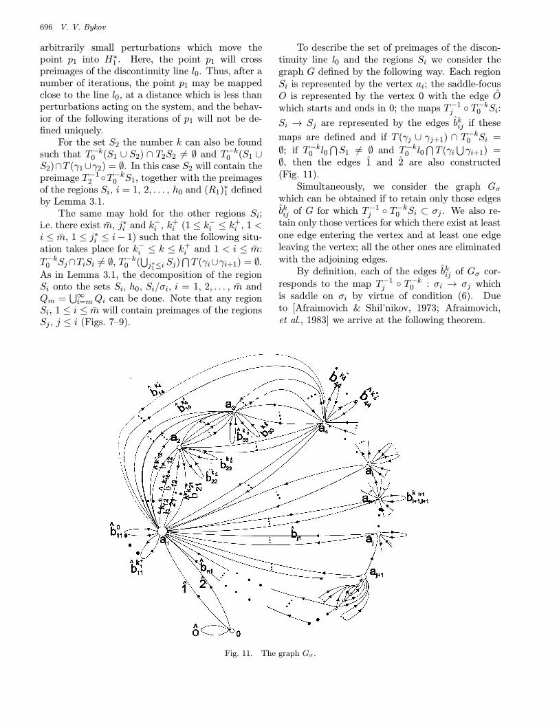
the line l0 and of the regions Si let us constructthe graph G, in which, following [Afraimovich &Shil’nikov, 1973], edges denote states, while vertices

denote transformations. Let each region Si corre-spond to a vertex ai, while the saddle-focus O corre-spond to an edge O, whose beginning and end formthe vertex 0; the maps T−1

j T−k0 Si: Si → Sj cor-

respond to edges bkij , if these maps are defined and

T (γj ∪ γj+1)∩ T−k0 Si = ∅ and, at last, the trajecto-ries, which are asymptotic to O as t→∞ and starton D at points belonging to T−1

1 l0 and T−k0 l0⋂Si,

correspond to edges 1 and 2 respectively, whichcome out from the vertex 0 and end at the vertexa1, if T−k0 l0

⋂S1 6= ∅ and T−k0 l0

⋂T (γi

⋃γi+1) = ∅.

Let us leave only those vertices which have at leastone incoming and outgoing edges, while we removethe rest of the vertices together with their start-ing edges. Consider the graph G and its subsetGσ, which contains only those edges bkij for which

T−1j T−k0 Si ⊂ σj .

Since, according to the construction, each of theedges bkij of the graph Gσ are determined by the map

T−1j T−k0 σi → σj, and regions σi are distinguished

by condition (6), then, in the same manner as in[Afraimovich et al., 1983; Shashkov & Shil’nikov,

1994] one can show that the map T−1j T−k0 gener-

ates the operator Tij: Hi(L)→ Hj(L) satisfying thesqueezed-map principle. Since the number of edgesin the graph Gσ does not exceed a countable set, wenumerate them so that each edge will correspondto a natural number. Let Ω denote the space ofall sequences of the form: (. . . , κi−1, κi, κi+1, . . .),where the symbol κi corresponds to the edges ofthe graph Gσ in such a way that two nearest sym-bols κi−1, κi denote edges, one of which ends andthe other starts at their common vertex. Then eachpoint ω = (. . . , κi−1 , κi0κi1 , . . .) in Ω is in one-to-one correspondence with a sequence of spaces andmaps

. . . , Hi−1

Ti−1i0−→ Hi0

Ti0i1→ Hi1, . . . .

Since all the spaces are complete and all operatorsare squeezing, then according to the lemma from[Shil’nikov, 1968] there exists a unique sequence ofcurves (. . . , hi−1 , hi0 , hi1 , . . .). This sequence weshall call the invariant stable fibre.

As follows from Lemma 3.1, the setsQ∗1⋃H∗1

⋃R∗1 give the adjoint intervals in S1 for the

Cantor discontinuum of the set S∗1 of stable fibers ofthe nontrivial hyperbolic set. Evidently, if p1 ∈ H∗1 ,then after some number of iterations the point p1

will lie below the line l0 and the next part of its orbitwill be defined by the map T−. If p1 ∈ S∗1 (i.e. ifit belongs to some stable fiber), then there exist

696 V. V. Bykov

arbitrarily small perturbations which move thepoint p1 into H∗1 . Here, the point p1 will crosspreimages of the discontinuity line l0. Thus, after anumber of iterations, the point p1 may be mappedclose to the line l0, at a distance which is less thanperturbations acting on the system, and the behav-ior of the following iterations of p1 will not be de-fined uniquely.

For the set S2 the number k can also be foundsuch that T−k0 (S1 ∪ S2) ∩ T2S2 6= ∅ and T−k0 (S1 ∪S2)∩T (γ1∪γ2) = ∅. In this case S2 will contain thepreimage T−1

2 T−k0 S1, together with the preimagesof the regions Si, i = 1, 2, . . . , h0 and (R1)∗1 definedby Lemma 3.1.

The same may hold for the other regions Si;i.e. there exist m, j∗i and k−i , k

+i (1 ≤ k−i ≤ k+

i , 1 <i ≤ m, 1 ≤ j∗i ≤ i− 1) such that the following situ-ation takes place for k−i ≤ k ≤ k+

i and 1 < i ≤ m:

T−k0 Sj∩TiSi 6= ∅, T−k0 (⋃j∗1≤i Sj)

⋂T (γi∪γi+1) = ∅.

As in Lemma 3.1, the decomposition of the regionSi onto the sets Si, h0, Si/σi, i = 1, 2, . . . , m andQm =

⋃∞i=mQi can be done. Note that any region

Si, 1 ≤ i ≤ m will contain preimages of the regionsSj, j ≤ i (Figs. 7–9).

To describe the set of preimages of the discon-tinuity line l0 and the regions Si we consider thegraph G defined by the following way. Each regionSi is represented by the vertex ai; the saddle-focusO is represented by the vertex 0 with the edge Owhich starts and ends in 0; the maps T−1

j T−k0 Si:

Si → Sj are represented by the edges bkij if these

maps are defined and if T (γj ∪ γj+1) ∩ T−k0 Si =

∅; if T−k0 l0⋂S1 6= ∅ and T−k0 l0

⋂T (γi

⋃γi+1) =

∅, then the edges 1 and 2 are also constructed(Fig. 11).

Simultaneously, we consider the graph Gσwhich can be obtained if to retain only those edgesbkij of G for which T−1

j T−k0 Si ⊂ σj . We also re-tain only those vertices for which there exist at leastone edge entering the vertex and at least one edgeleaving the vertex; all the other ones are eliminatedwith the adjoining edges.

By definition, each of the edges bkij of Gσ cor-responds to the map T−1

j T−k0 : σi → σj whichis saddle on σi by virtue of condition (6). Dueto [Afraimovich & Shil’nikov, 1973; Afraimovich,et al., 1983] we arrive at the following theorem.

Fig. 11. The graph Gσ.

On Bifurcations Leading to Chaos in Chua’s Circuit 697

Theorem 3.1. The system Xµ has a nontrivial hy-perbolic set which is in one-to-one correspondencewith the set of infinite paths along the edges of Gσ.

The next theorem shows the nontrivial char-acter of the bifurcational set on the parameter µplane.

Theorem 3.2. There exists a countable set of bi-furcational curves corresponding to the presence ofhomoclinic loops of the saddle-focus O and a Cantorset of bifurcational curves corresponding to the sit-uation where the one-dimensional separatrix of thesaddle-focus lies on the stable manifold of a non-trivial hyperbolic set.3

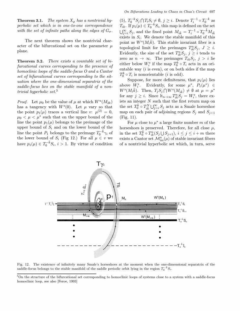
Proof. Let µ0 be the value of µ at which W u(M2k)has a tangency with W s(0). Let µ vary so thatthe point p1(µ) traces a vertical line v: µ(2) = 0,µ0 < µ < µ∗ such that on the upper bound of theline the point p1(µ) belongs to the preimage of theupper bound of Si and on the lower bound of the

line the point P1 belongs to the preimage T−k0 γi ofthe lower bound of Si (Fig 12.) For all µ ∈ v we

have p1(µ) ∈ T−k0 Si, i > 1. By virtue of condition

(5), T−k0 Sj⋂TiSi 6= ∅, j ≥ i. Denote T−1

i T−k0 asTik. If p1(µ) ∈ T−k0 Si, this map is defined on the set⋃∞j=i Sj, and the fixed point Mik = T−1

i T−k0 Mik

exists in Si. We denote the stable manifold of thispoint as W s(Mik). This stable invariant fiber is atopological limit for the preimages TnikSj , J ≥ i.Evidently, the size of the set TnikSj, j ≥ i tends tozero as n → ∞. The preimages TikSj, j > i lieeither below W s

i if the map T k0 Ti acts in an ori-entable way (i is even), or on both sides if the mapT k0 Ti is nonorientable (i is odd).

Suppose, for more definiteness, that p1(µ) liesabove W s

i . Evidently, for some µ∗, P1(µ∗) ∈W s(Mik). Then, TjSj

⋂W s(Mik) 6= ∅ at µ = µ∗

for any j ≥ i. Since ltn→∞ TnikSj = W si , there ex-

ists an integer N such that the first return map onthe set T k0 TNik

⋃∞j=i Sj acts as a Smale horseshoe

map on each pair of adjoining regions Sj and Sj+1

(Fig. 11).For µ close to µ∗ a large finite number m of the

horseshoes is preserved. Therefore, for all close µ,in the set T k0 Tnik(Sj

⋃Sj+1), i ≤ j ≤ i +m there

exists a Cantor setMnim(µ) of stable invariant fibers

of a nontrivial hyperbolic set which, in turn, serve

Fig. 12. The existence of infinitely many Smale’s horseshoes at the moment when the one-dimensional separatrix of thesaddle-focus belongs to the stable manifold of the saddle periodic orbit lying in the region T−k0 Si.

3On the structure of the bifurcational set corresponding to homoclinic loops of systems close to a system with a saddle-focushomoclinic loop, see also [Feroe, 1993]

698 V. V. Bykov

as limits for sequences of the lines Lnim of preimagesof the discontinuity line l0. When µ varies, the pointp1(µ) intersects all these lines and each intersectioncorresponds to one of the bifurcations prescribed bythe theorem. The theorem is proved.

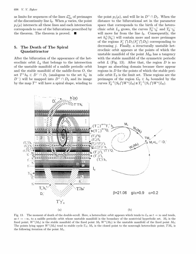
5. The Death of The SpiralQuasiattractor

After the bifurcation of the appearance of the het-eroclinic orbit Lg that belongs to the intersectionof the unstable manifold of a saddle periodic orbitand the stable manifold of the saddle-focus O, theset T+h0 ∈ D− ∩ D1 (analogous to the set h−0 inD−) will be mapped into D+ ∩ D2 and its imageby the map T+ will have a spiral shape, winding to

the point p1(µ), and will lie in D+ ∩D1. When thedistance to the bifurcational set in the parameterspace that corresponds to the birth of the hetero-clinic orbit Lg grows, the curves T+

0 γ+0 and T−0 γ

−0

will move far from the line l0. Consequently, theset h+

0 (h−0 ) will contain more and more preimagesof the regions S−j

⋂D1(S+

j

⋂D2) corresponding to

decreasing j. Finally, a structurally unstable het-eroclinic orbit appears at the points of which theunstable manifold of the point M02 has a tangencywith the stable manifold of the symmetric periodicorbit L (Fig. 13). After that, the region D is nolonger an absorbing domain because there appearregions in D for the points of which the stable peri-odic orbit Γ0 is the limit set. These regions are thepreimages of the region G0 ∈ h0 bounded by thecurves T−1

0 (S0⋂W s(L0) II/ T−1

1 (S1⋂W s(L0).

(a) (b)

Fig. 13. The moment of death of the double-scroll. Here, a heteroclinic orbit appears which tends to L0 as t→∞ and tends,as t → −∞, to a saddle periodic orbit whose unstable manifold is the boundary of the nontrivial hyperbolic set. M0 is thefixed point; W s(M0) is the stable manifold of the fixed point M0 W

u(M0) is the unstable manifold of the fixed point M0;The points lying upper W s(M0) tend to stable cycle Γ0; Mh is the closed point to the nonrough heteroclinic point; TMh isthe following iteration of the point Mh.

On Bifurcations Leading to Chaos in Chua’s Circuit 699

Acknowledgments

This research was supported in part by grantINTAS-93-0570 and the Russian Fundation ofFundamental Research (grants 97-01-00015 and98-02-16278).

ReferencesArnold, V. I. [1982] Geometrical Methods in the The-

ory of Ordinary Differential Equations (Springer, NewYork).

Afraimovich, V. I. & Shil’nikov, L. P. [1973] “The singu-lar sets of Morse-Smale systems,” Tran. Mosc. Math.Soc. 28, 181–214.

Afraimovich, V. S., Bykov, V. V. & Shil’nikov, L. P.[1977] “On the appearance and structure of Lorenzattractor,” DAN SSSR 234, 336–339.

Afraimovich, V. S., Bykov, V. V. & Shil’nikov, L. P.[1983] “On the structurally unstable attracting limitsets of Lorenz attractor type,” Tran. Mosc. Soc. 2,153–215.

Afraimovich, V. S. & Shil’nikov, L. P. [1983] StrangeAttractors and Quasi-Attractors in Nonlinear Dynam-ics and Turbulence, eds. Barenblatt, G. I., Iooss, G. &Joseph, D. D. (Pitman, New York), pp. 1–28.

Afraimovich, V. S. & Shil’nikov, L. P. [1983]“Invariant two-dimensional tori, their breakdownand stochastisity,” in Methods of Qualitative Theoryof Differential Equations, ed. Leontovich-Andronova,E. A. (Gorky Univ. Press) (translated in Amer. Math.Soc. Trans. 149(2), 201–212.

Belykh, V. N. & Chua, L. O. [1992] “New type of strangeattractor from geometric model of Chua’s circuit,” Int.J. Bifurcation and Chaos 2, 697–704.

Belyakov, L. A. [1984] “Bifurcation of systems withhomoclinic curve of saddle-focus,” Math. Notes Acad.Sci. USSR 36(1/2), 838–843.

Chua, L. O., Komuro, M. & Matsumoto, T. [1986]“The double-scroll family,” IEEE Trans. CircuitsSyst. CAS-33(11), 1073–1118.

Chua, L. O. & Lin, G. [1990] “Intermittency in piecewise-linear circuit,” IEEE Trans. Syst. 38(5), 510–520.

Dmitriev, A. S., Komlev, Yu. A. & Turaev, D. V. [1992]“Bifurcation phenomena in the 1:1 resonant horn forthe forced van der Pol-Duffing equations,” Int. J.Bifurcations and Chaos 2(1), 93–100.

Feroe, J. A. [1993] “Homoclinic orbits in a parametrizedsaddle-focus system,” Physica D62(1–4), 254–262.

Freire, E., Rodriquez-Luis, A. J., Gamero, E. & Ponce,E. [1993] “A case study for homoclinic chaos in an au-tonomous electronic circuit,” Physica D62, 230–253.

Gavrilov, N. K. & Shilnikov, L. P. [1973] “On three-dimensional systems close to systems with a struc-turally unstable homoclinic curve,” Math. USSR Sb.17, 446–485.

George, D. P. [1986] “Bifurcations in a piecewice linearsystem,” Phys. Lett. A118(1), 17–21.

Harozov, E. I. [1979] “Versal unfolding of equivariant vec-tor fields for the cases of the symmetry of the secondand third orders,” Trans. I. G. Petrovsky’s Seminar5, 163–192 (in Russian).

Khibnic, A. I., Roose, D. & Chua, L. O. [1993] “On peri-odic orbits and homoclinic bifurcations in Chua’s cir-cuit with smooth nonlinearity,” Int. J. Bifurcation andChaos 3(2), 363–384.

Lozi, R. & Ushiki, S. [1991] “Confinor and bounded-timepatterns in Chua’s circuit and the double-scroll fam-ily,” Int. J. Bifurcation and Chaos 1(1), 119–138.

Lozi, R. & Ushiki, S. [1993] “The theory of confinorsin Chua’s curcuit: Accurate analisis of bifurcationsand attractors,” Int. J. Bifurcation and Chaos 3(2),333–361.

Madan, R. N. [1993] Chua’s Circuit: A Paradigm forChaos (World Scientific, Singapore).

Newhouse, S. E. [1979] “The abundance of wild hyper-bolic sets and nonsmooth stable sets for diffeormor-phism,” Publ. Math. IHES 50, 101–151.

Ovsyannikov, I. M. & Shil’nikov, L. P. [1987] “On sys-tems with a saddle-focus homoclinic curve,” Math.USSR Sbornik 58, 91–102.

Shashkov, M. V. & Shil’nikov, L. P. [1994] “On existenceof a smooth invariant foliation for maps of Lorenztype,” Differenzial’nye uravnenija 30(4), 586–595 (inRussian).

Shil’nikov, L. P. [1968] “On a Poincare–Birkgoff prob-lem,” Math. USSR Sborn. 3, 353–371.

Shil’nikov, L. P. [1970] “A contribution to the problem ofa rough equilibrium state of saddle-focus type,” Math.USSR Sbornik 10, 92–103.

Shil’nikov, L. P. [1991] “The theory of bifurcations andturbulence 1,” Selecta Math. Sovietica 1(10), 43–53.

Shil’nikov, L. P. [1994] “Chua’s circuit: Rigorous resultsand future problems,” Int. J. Bifurcation and Chaos4(3), 489–519.