__ _EVELZ.__

Technical Report 562

41

M. Taylor

Analysis of A

Direct Mechanical Stz.bilization Platform Ifcr Antenna Stabilization and Control

in a Shipboard Environment

25 March 1981

Prepared for the Department of the Navy

under Electronic Systems Division Contract FI%28-80-C-0002 by

Lincoln LaboratoryMASSACHUSEMTS INSTITUTE OF TECHNOLOGY I-I

D.;xI/vGrO.N, MA.sA Gltt Ž•:;T• -

DT 1C Approved for public release; distribution unlimited.

EL-EC-IT

JUN 2 3 1981H Jio

The work repoi:ed in this document was performed at Lincoln Laboratory, acenter for research operated by Massachusetts Institute of Technology. Thework was sponsored by the Department of the Navy under Air Force ContractF19628-80-C-0002.

This repozt may be reproduced to satisfy needs of U.S. Government Agencies.

The views and conclusions contained in this document are those of the con-tractor and should not be interpreted as necessarily representing the officialpolicies, either expressed or implied, of the United States Government.

This technical report has been reviewed and is approved for publication.

FOR THE COMMANDER

Raymond L. Loiselle, Lt.Col., USAFChief, ESD Lincoln Laboratory Project Office

Non-Lincoln Recipients

PLEASE DO NOT RETURN

Permission Is given to destroy this document

when it is no longer needed.

MNASSACI- RISETTS INSTITUTE OF TECH NOLO)(;Y

I.INCOI.N LABORATORY

ANNALYSIS OF DIRECT MECHANICAL STABILIZATION PLATFORM

FOR ANTENNA STABILIZATION

AND CONTROL IN A SHIPBOARD ENVIRONMENT

1/. 7"-) 1,0R

A~e .... ion ForCP',i G A& I

DTIC TAB L]Un~ann oun ced EJu-t if ic~tition-ID

TECHNICAL REPORT 562-

DDiztribut ion/

Availability Codes25 MARCH 1981 Avail..n./or':Avail and/or

Dint Spcc ial

Approved for public release; distribution unlimited.

I.EXINGTON MASSACHUSETTS

rr -

Abstract

This report presents a rigid body analysis of the dynamics

of a shipboard antenna in a three-axis gimbal configuration

utilizing Direct Mechanical Stabilization (DMS) for primary

It control. System parameters are defined and Euler equations

applied to obtain a non-linear system model that includes

expected torque inputs. A computer simulation is generated

with ship input motions due to roll, pitch, turn and flexure

and a numerical integration procedure is then employed to

determine the motion of the antenna and the resulting pointing

error for various scenarios.

The results of the cases studied indicate potential feasi-

bility of this approach for applications requiring pointing

accuracy of approximately ±0.15 degree.

CONTENTS

Abstract iii

List of Illustrations vi

1.0 INTRODUCTION 1

2.0 KINEMATIC FRAMES & EULER ROTATIONS 6

3.0 ANGULAR VELOCITIES 10

4.0 STATE VARIABLES 12

5. 0 GYRO EULER EQUATIONS 13

6.0 PLATFORM EULER EQUATIONS 14

7.0 CONSTRAINTS 14

8.0 TRANSFORMATIONS & CONTROL OF 8x, y, T 15

9.0 TORQUE EQUATIONS 21

10.0 SYSTEM EQUATIONS 30

11.0 COMPUTER SIMULATION 33

APPENDICES

A. Euler Equations for Gyros and Platform 41

B. Constraints 45C. Transformations for exc and y 47D. Acceleration Vector and Torque Due to Unbalance 50

E. Generation of System Equations (10-1) and (10-2)for 0 and 8 57x y

F. Generation of System Equations (10-5), (10-6), and

(10-7) for wp3 wpl', and wp2 62

G. Generation of p2 from Velocity Constraints 71H. Computer Programs 74

References 81

Nomenclature 82Terms in Solutions 86

vIIVi

LIST OF ILLUSTRATIONS

1. X-Y DMS Pedestal Picture 3

2. X-Y DMS Components and Structure 5

3. X-Y DMS Kinematic Frames 7

4. X-Y DMS Control Outline 18

5. X-Y DMS Commands 19

6. X-Y DMS Error (Rolling) 36

7. X-& DMS Gyro Motion (Rolling) 37

8. X-Y DMS Error (Roll, Pitch, Turn) 39

9. X-Y DMS Gyro Motion (Roll, Pitch, Turn) 40

H-I Computer Flow Diagram 75

vi

vi

1.0 INTRODUCTION

This i- -le rigid body analysis of a DMS*-controlled

antenna on board a surface ship for a three--axis gimbal con-

figuration employing X-Y over train. The combined effects of

roll, pitch, turn maneuvers and ship flexure on the pointing

accuracy of the antenna are studied.

1.1 Background

The gyroscope has found its most prolific application in

modern technology as an angular direction and motion sensor

whose electrical output signal is used to activate either amechanical or computational device. However, throughout the Ilast half century of very active development and refinement of

these sensors of shrinking size, there has been a lower level

but continuing effort on large gyro wheels for DMS. The most

sophisticated effort on DMS in recent years has been associatedwith the use of control moment gyros for stabilization and atti-tude control of satellites.

There are two general approaches to the concept of DMS:

1) Mount the stabilized device directly to the frame carrying Ithe gyro rotor. This assembly is then mounted within gimbals

and bearings to permit angular isolation from input motion.

Examples of this approach are found in both early and more

recent literature. Scarborouh1 describes the gyro pendulum;

Williams(2) analyzes stabilization of an optical sensor for a

shipboard application; Bieser(4) describes a configuration of

this type for stabilizing an antenna on board a ship.

Direct Mechanical Stabilization

S • ±W ! • • "• " • V • ! • , • ! i • .• •. • • , , • •',XL1

, .- -- -,.

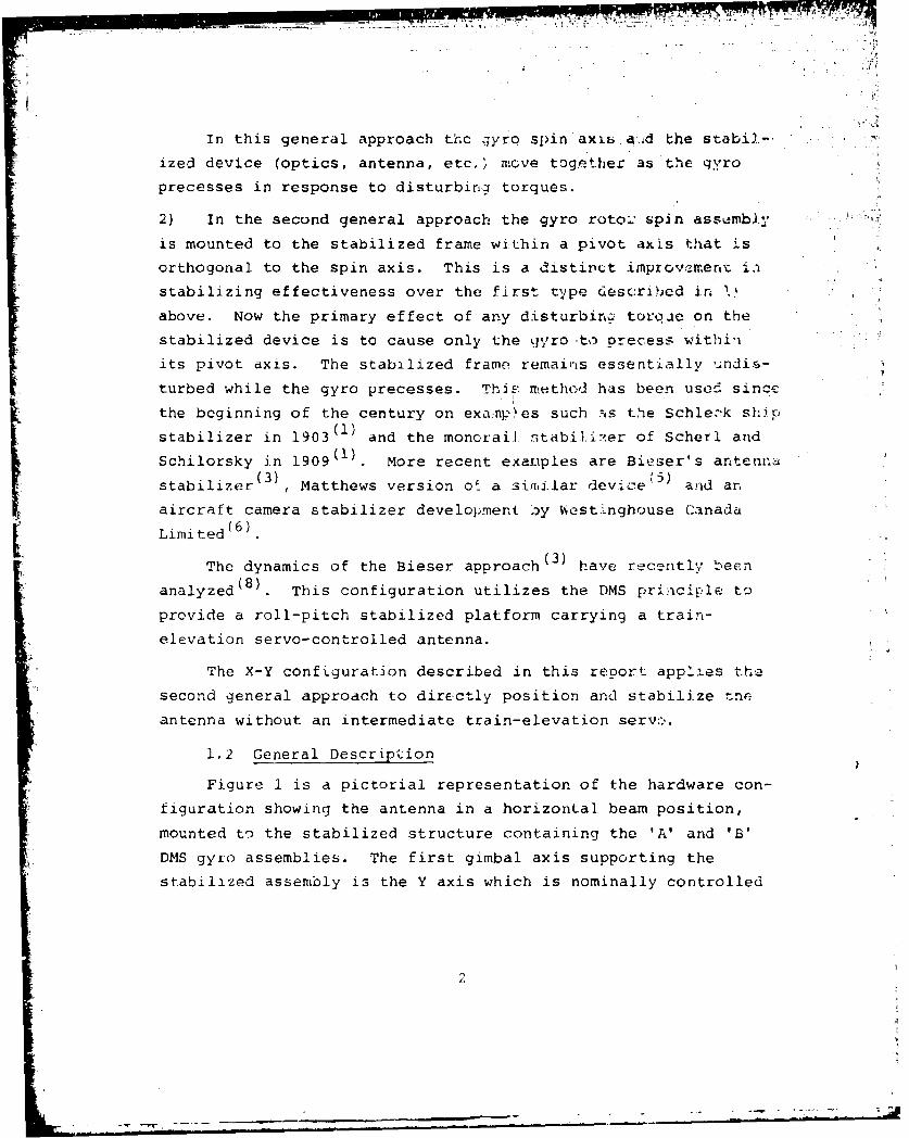
In this general approach the ..Tyro spin axis.aa .d the stabi)-'

ized device (optics, antenna, etc.) move together as the qyroprecesses in response to disturbirnci torques.

2) In the second general approach the gyro rotor" spin ass,.nmb..

is mounted to the stabilized frame within a pivot axis that is

orthogonal to the spin axis. This is a distinct improvrzment iLi

stabilizing effectiveness over the first type described in '..

above. Now the primary effect of any disturbing tor'que on the

stabilized device is to cause only the Litro to precess withinits pivot axis. The stabilized frame remains essentially .indis-

turbed while the gyro precesses. ThjE' method has been used since

the beginning of the century on exa~npý,es such Tts the Schlezk shirp

stabilizer in 1903(1) and the monorail stabiliz'er of Scherl and

Schilorsky in 1909(1). More recent examples are Bieser's antenna-

stabilizer(3) Matthews version ol- a sistilar device 5) aid an

aircraft camera stabilizer development o.y %estinghouse Canada

Limited (6)

The dynamics of the Bieser approach(3) have recently been

analyzed(8). This configuration utilizes the DMS princip-le to

provide a roll-pitch stabilized platform carrying a train-

elevation servo-controlled antenna.

The X-Y configuration described in this report applies the

second general approach to directly position and stabilize the

antenna without an intermediate train-elevation servw.

1.2 General Description

Figure 1 is a pictorial representation of the hardware con-

figuration showing the antenna in a horizontal beam position,

mounted to the stabilized structure containing the 'A' and 'B'

DMS gyro assemblies. The first gimbal axis supporting thestabilized assembly is the Y axis which is nominally controlled

2.

! • • • : ... •~~~ • - .- . . . .

r-ANTýNNA

Y-AXIS "

A-GYR O -Gs

X- AX IS

..- '--I RAIN PICKOFF

T R A I N-- -"

STEPPER .- --MOTOR

Fig. i. X-Y DMS pedest.l pi.t.'re.

to be in the vert.ical plane containing the satellite; the ncxt

supporting a.,.is is the X axis which is nominally controlled to be

perpendicuiar tc the vertical plane containing the satellite. The

total assembly is carried on the train axis which is mounted to

the deck or the shlo.

Further *d.etail is given in Figure 2 where the antenna is

shown in a verti-zal beam position. The 'A' gyro is free to pivot

about &n axis parallel to X and the 'B' gyro is free to pivot

abouL an axis pat-allel to Y. The gyro pivot axes and the X, Y

cir.Laal. axes are each equipped with a torquer and angular pickoff.

'T'he train axis is positioned by a stepper motor, and has a pre-

ci-e angular pickoff to read its position.

Antenna beam position control is achieved by applying appro-

•riate fontzol torqu..s to the 'A' or 'B' gyro torquer. For

e'camplef, antenna i'cticn about the X axis is achieved by applying

a horque to the 'I' gyco torquer. The antenna is stabilized

acaio--t the effects of disturbing torques by precession of the

•gyo assem.blies within thcir respective pivot axes. Narrow band-

width :agi;ig loops, are used to maintain the spin axes nominally

[paral.lel to the antenna be-am axis. For example, the X torquerresponds to a plck-ff signal from th.e 'B' gyro to null the 'B'

gyro picxcff o0,tp'41-.

rthe d.toaj.ls of the control concep.s will be explained in the

bý.dy of this repoy.t.

4t

X-TORGUER

ANTENNA

"AB GYYOO

TORQUER

SY- PICKOFFnB' D'ISC; Y RIO/ "A" GYROASS', PICKOFF

/ 1 /"A"1 GYRO"B" GYRO IPICKOFF

Y- TORQUERA' D.IS

XPICKOFF As

-TRAINSTEPPER

TRAIN PICKOFF MOTOR

r

Fig. 2. X-Y DMS components and structure.

m - -- - - - - - - --- ---

2.0 KINT'MATIC FRAMES & EULER ROTATIONS

Referring to Figure 3, the following reference frantes andtheir Euler rotations are defined;

{n} = inertial frame

{•} = deck frame

{P} antenna platformA F

{aI = 'A' gyro gimbal

{•} ='B' gyro gimbal

{e} = frame containing satellite position along 12

Ag} = X-Y gimbal frame iiAdditional intermediate reference frames are defined below in IIterms of the angles of rotation and the axis of each rotation. ii

= ship azimuth

Ip = pitch

ýR = roll I

tH= heel (YRH =R + H)

e = train

6 = X axisxey = Y axis •

= gyro 'A' gimbal rotation with respect to platform

Y b = gyro 'B' gimbal rotation with respect to platform

otA = satellite azimuth position

LE satellite elevation position

b- \

z

N.

>4-

r

-1 E4

cc

<77

< 12. Cb

;-l

The format for showing the rotation sequences are:

starting Rotation Angle iframe afterl Iiframe Rotation Axis rotation

Applying this fornat and the previously defined frames and rota-

tion angles the rotation sequences are as follows:

Deck of Ship

1A P RHA { .AA_n - n} - {f)

AA A,11,

A

Antenna Platform Ap I

AT A xy

A A A

i3 23

"A' Gyro {a}

• YaA

-4" {alA

P-1

8

'B' Gyro (b}

A@Yb ^

A3-

Satellite Position Vector Along {e2-

A cA A aE Aj

A A,113 ej-l 9

9:

3.0 ANGULAR VELOCITIES

The following angular velocities are defined:

Deck of Ship {f}

A A A

f+f (3-1)-f= Afl f + f2 f22 + Rf3 f3 (3-2)

Antenna Platform {P}

A A APl + p22 p33

* A * A * A

-P -+ T - 6. Sl + y E3 (3-4)

'A' Gyro {a}

A A AGimbal: W Wa1 a +w a + w a (3-5)-a al -1 a2 -2 a3 -3

A A ARotor: -- a W al al + £a a2 + wa3 a3 (3-6)

where a = constant wheel spin speed

Note that 'a = Wal -wpl

10

r ^ -_•T~

'B' Gyro Ab}

A A A

Gimbal: •-b = blb + wb2 12 + wb3 b3 137)

A A A

Rotor: (3-b)Rb b l b "b b2 + wb3 b 3 (3-8)

A

Note that the polarity of Sb b2 is negative. This is essential

to assure that both rotors precess in the same direction with

the antenna when a control torque is applied to either rotor.For example the torquer used to control X axis motion applies aAtorque to the 'B gyro about coand, via reaction, an opposite

AApolarity torque to the 'A' gyro about a3. Both rotors then o sA

precess in the same direction about bI adAI r s et vl wh e

the antenna moves about pl.

Note that )-b = wb3 -Wp3"

11

11I

4.0 STATE VARIABLES

The following state variables are defined for the system

equations that will be developed:

X = xx72= .e

Sy

X3 = al

4 b3

5 p3

6 = p

X7 p2

x =Y8 a

X = bdt10 a

X 11= fyadt

x12 = eT T

x = eT

I-3 T

12

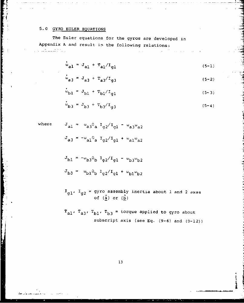
5. 0 GYRO EULER EQUATIONS

The Euler equations for the gyros are developed inAppendix A and result in the following relations:

•al = Jal + T al/Igl (5-1)=J + T /1 (5-1)

a a3 a3/ g3a3 +T /1 (5-2)

Wbl Jbl + Tbl/Igl

Wb3 Jb 3 + Tb3/Ig3 (5-4)

where Jal = 'a3Pa Ig2/Igl - Wa3'a2

Ja 3 =-al Qa Ig2/Igl + Walwa2

Jbl =-u'b3 0b Ig2/Igl - wb3wb2

Jb3 = Wbl Qb Ig2/Igl + Wbl'b2

1 gI, 'g2 = gyro assembly inertia about 1 and 2 axesof {a} or {b}

Tal' Ta3' Tbl' Tb 3 = torque applied to gyro about

subscript axis (see Eq. (9-6) and (9-12))

13

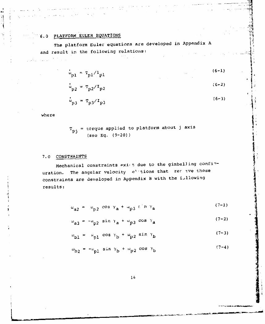
6.0 PLATFORM EULER EQUATIONS

The platform Euler equations are developed in Appendix A

and result in the following relations: -4

I

T /T (6-1)

Wp2 pTp2 /Ip 2 (6-2) p2

p3 Tp 3 /ipa. 3 (6-3) ip3 T 3/Ip

where I

T torque applied to platform about j axis

(see Eq. (9-20))A

7.0 CONSTRAINTS

Mechanical constraints Pxi, t due to the gimbal)ing confi"-

uration. The angular velocity el'tions that rer rve these Iconstraints are developed in Appendix B with the i.llowing

results:

a2 COB Sa + u 'n ya (7-1) ia a2 Wp2 a p3 a-

La 3 = -wp2 sin a + W p 3 COS ).a (7-2)

W bl W Ul Cos b + Wp2 sin yb (7-3)

" "b2 =-Wpl sin Yb + (0p2 Cos Yb (7-4)

14

?j

.8.0 TRANSFORMATIONS AND CONTROL OF x e 6

8.1 Transformation for 9 , and 8YA

The antenna beam lies along axis the satellite position

vector lies along 2 We desire to orient P2 coincident with 2

using the rotations defined in Section 2.0 to determine appro-

priate input command angles 8 and 6yc as functions of A, aE,,

1PA' ýp'lRH' eT The computation process determines the {n}

components of and e2' then equates these components to solve

for e and 6xc yc

The direction cosine matrices for the rotations in Section

2.0 are defined using the symbols,

[Ci(C)] = Direction cosine matrix for rotation

about i th axis of starting frame

through the angle i.

Using this notation the reldtions between various reference

frames are defined as follows:

A

{f'} [ 3 () I [C2 (tP) I [C1 (OP) ] [C3 ) ] )

L A,

If' } [B

{.} = [C3 [C1 ) ] {f' i

A (8-2)

A I fl151

i. ,15 3

{ f [C 1 (ya) l•_ (8-3)

AAA{b} = [c3(Yb)]}�) (8-4

AA(e_ = [c E (E)I[C 3 (cA)]{n} (8-5)

From (8-1) and (8-2)

A{P} (B [B2B ]n}_ (8-6)

T T A{n} = BT BT {pB 1 B2 (

From (8-5)

BT} (8-7)

A A ASThe n components of P2 and e_2 are now equated using (8-6) and(8-7)

T T T iB B1 B 1 (8-8)

16

F IThe expansicn and solution of Eq. (8-8) for the desired angles

is performed in Appendix C with the following results:

V 4c sin 1-t (8-9)

= sin (t 3 /cose () 10)

where

ti, t 3 results of matrix equation (C-3) in

Appendix C.

8.2 Systen Control

The control approach that will be used to achieve the

desired values ' y is shown in Figures 4 and 5.S~Xc' yc

Referring to Figure 4, the command values eXc', yc are

compared to actual values measured by the X, Y pickoffs and

the error signals drive the appropriate gyro torquers. A

train command based on ship's heading and satellite position

(see Figure 5 and Section 8.3) drives the train stepper motor.

The bottcer loop shown in Figure 4 is a 'housekeeping' loop thatkeeps the gyro spin axis nominally parallel to the antenna beamaxis.

Figure 5 shows the flow of information used to generate

the control commands. The ship's master compass and heading

reference provide roll, pitch and heading information used in

the coordinate transformations. The heading output of the

compass is also utilized directly to position the train servo.

17

LJ

On, ..c Y+ GYROTRANSFER .x #H Y

CO~M ANDS -- .TORQUERSI FUNCTION

COMMANDS " T OR|IKO_

TRAIN POSITION LOOP

X,Y TORQUERS FNTO

GYRO CAGING LOOPS

NOTE: THERE IS NO ACTIVE STABILIZATION LOOP. THE GYROSPROVIDE THIS FUNCTION. -

Fig. 4. X-Y DMS control outline.

18

[I

- .- -- - --

, 44

jTR'562(5) 1

TRAIN

SHIP FLEXURE COMMANDSHIP'Sý IROLL +., +

COMPASS I PITCH&

iTATITUDE I HEADINGTIIATTREFERENCEl RI

N

- F( +, 0 I X, Y

+ RDESI RED M I COMMANDS

AZIMUTH DESIRED AEPHEMERIS +AZ-EL TI

+ POSITION I I

TRACKING 0

•;/ERRORN

TRAIN PICKOFF

Fig. 5. X-Y DMS commands.

119

• ,•- ~ -~ - -- •: -- -- - • -'... .. . . ._.... ... .• _-".=. ,.-. :

The satellite ephemeris data is updated by d-wn-link tracking

error signals to provide the desired antenna beam position to

the satellite. The coordinate transformation computation gen- Aerates the desired values 0 a based on the inputs shown. A

The basic stability of the DMS gyros permits a narrow band-

width control from the command signals to the gyro torquers. 4

This attenuates or filters the effect of high frequency ship

flexure on the controlled output. Long term flexure due to

thermal effects or loading are corrected by the down-link track-

ing error.

8.3 Train Axis Control of 9T

The purpose of the train axis is to nominally position the

Y axis in the vertical plane containing the satellite. This is

not a critical requirement and so it is expected that an inex-

pensive stepper motor will be used in train. For the purpose

of modelling, the following damped second order system has been

assumed in train:

S+ 2w + W a2 a w2 A (8-11)n nA

where

i • = '•A+ 0 T :

.w = natural frequency of train servon

= damping factor

•A azimuth position of satellite

A

20 -|

i -:

Making the substitution for 8 as indicated above leads to the

defining equation for e

T' 2

T + 2w 4 + W T= F (8-12)T n T nTA

A-where 4 i

2-'A n + WnA-*AI )

9.0 TORQUE EQUATIONS

In this section the torque contributors that produce the

system response are defined for computational purposes:

9.1 Gyros 'A' and 'B' TorquesS-"

Spring

Friction

Unbalance I

Bias

Control

Bearing Reaction

I Total

21

Platform Torques ISpring

FrictionIiUnbalance

Bias A

Gyro Reaction

Bearing Reaction

Control ]Total

9.2 Gyro 'A' Torques

9.2.1 Spring

An elastic spring torque due to rotation of the 'A' A-_Agyro about its pivot axis, a1 is modelled.

T =K (9-1)

-as -KsGYaal (- I

where

KsG = gyro spring gradient

9.2.2 Friction

Friction about the pivot axis is modelled as a constantmagnitude torque with a polarity that opposes the relativeangular velocity of the 'A' gyro with respect to the platform.

22

TaI a (9-2)

where

KFG gyro friction torque amplitude

9.2.3 Unbalance

Torque about the pivot axis due to unbalance has been

modelled as a displacement along the rotor spin axis, 92' coupled

with transverse acceleration components. Unbalance torque due to

radial displacement along 3 has been assumed to be insignificantin recognition of the fact that radial stability of balance is

much better than axial stability. See Appendix D (Eq. (D-14))

for development of this expression.

Tau =-mi [-A2sinya + A3cosy a (9-3)

where m = gyro mass

z9 = displacement of gyro mass center from centergAof support along •2

A2 ,A3 = acceleration components along and A

respectively

9.2.4 Bias

Bias torque has been modelled about the pivot axis.

=T A (9-4)-aB aB -l

23

j7

where ,

C1

TaB = bias torque value

9.2.5 Control

Referring to Figure 3, the control torque on the 'A' gyro

is exerted about the pivot axis a to correct for Y axis error A

as indicated by the difference between the command value, Oyc,'

and the actual value, e Recall from Figure 5 that the command

angle computation is degraded by ship flexure between the master

attitude reference and the deck at the antenna. A conservative

worst-case situation is modelled with the full ship flexure

-Amplitude introduced into the control equation.

TCa a( -Oy + F)l a (9-5)

where

K = control gain (in-lb/rad)a

0 ship flexure arplitude (rad)

9.2.6 Bearing Reaction

Radial forces at the pivot bearings introduce torquetA A tA

about a and a3. The component about a 2 has no significant

effect since a2 is along the spin axis of the rotor. Accord-ingly, the torque due to bearing reaction is defined as:

T mT A (9-6)!Ra a3 -3

24

II

where

Ta 3 = magnitude of bearing reaction torque (in-lb)

9.2.7 Total Torque on 'A' Gyro

The total torque on the 'A' gyro is

A A ATa =T al + T a2 +ATa3 a3 (9-7)

where

Tal = -as + TaF + -au + TaB + TcA

T = 0a2

9.3 Gyro 'B' Torques

The torques acting on the 'B' gyro are similar to those on

the 'A' except for different axes and a geometric consideration

applied to the control torque.

9.3.1 Spring

ATbs = sGb b(9-8)

9.3.2 Friction

ATbF = -KyFG[b/y'bl] b3 (9-9)

25

9.3.3 Unbalance

STbu =-mtg[AlCOSYb + A2 sinYb] 19-10)

See Eq. (D-19) in Appendix D.

9.3.4 Bias

ATbB T b3 (9-11)

9.3.5 Contrcl

A

TCb = -Kbxc -x + eF)cosey b 3 (9-12)

Note that the control torque is responsive to the antenna

error signal about the X axis with ship flexure again introducedas a worst-case effect. Any displacement in Y serves to increase

the X rate response to a given torque input. This is offset by

introducing cosey into Eq. (9-12).

9.3.6 Bearing Reactiox.Following similar arguments to that in 9.2.6, we write

ATRb T bI (9-13)

26

r --

9.3.7 Total Torque on 'B' Gyro

The total torque on the 'B' gyro is.

A Alb " Tb -l + Tb 3 -3 (9-14) -I

where

I~Ii"T b3 13 lbs + TF+Ibu T bB + Tb

9.4 Platform Torques

9.4.1 Spring

Spring torque acting on the platform is a function of8 and y displacement. Spring torque due to e is cancelledx y Tout by the stepper motor. i

A AT =-K [e •x + e (9-15)-ps p x 1 y 3

where K = spring gradientsp

9.4.2 Friction

Friction is modelled as a constant amplitude torque with

a polarity in opposition to velocities e and yx y,

TpF = A[X l + {ey/II) -3] (9-16)

27

9.4.3 Unbalance

The platform unbalance torque is defined in Section D-10

of Appendix D with the result --

A A AT-pu •Tul E1 + Tu2 P2 + Tu3 (3 (9-17)

where

T Mul (A2 3 A3 2)

Tu2 =M (A32k1 - A12X3 )

T MAu3 1(AI 2 -2

M = platform mass

A. = displacement of mass center along P2i axis

9.4.4 Bias

AAT =TBx g1 + T 3 (9-18)-pB TxBYP-

where TB, T = bias torque about X and Y axes

9.4.5 Gyro Bearing Reaction

The total torques acting on the 'A' and 'B' gyros are

defined as Ta and Tb in Eqs. (9-7) and (9-14) respectively.

These are primarily reaction torques between the gyros and the

platform except for the gyro unbalance torques which are small.

28

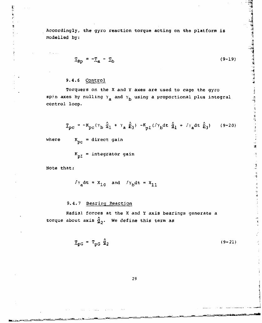
Accordingly, the gyro reaction torque acting on the platform is

modelled by:

TRp -Ta -Tb (9-19)

9.4.6 Control

Torquers on the X and Y axes are used to cage the gyro

spin axes by nulling y a and yb using a proportional plus integral

control loop.

TPc =-Kpc (Y + Ya 3) A -KI(fYbdt A + fYadt A3) (9-20)

where K = direct gainPC

K =integrator gainpI

Note that:

fYadt =X10 and fybdt X X1

9.4.7 Bearirg Reaction

Radial forces at the X and Y axis bearings generate aA =

torque about axis A We define this term as

A

TpG TpG A2 (9-21)

29

I

S9.4.8 Total Platform Torque .. .1

Sum the previously defined torque contributions to deter- Imine the total platform torque: .A

or in terms of frame components,

A A A KT= TPlp1 + T + T 3 (9-23)--p Tpp2 E 2 Tp3 R

10.0 SYSTEM EQUATIONS1-4

The system equations are generated in the Appendices andare summarized below followed by a description of their develop-

ment process.

x= pl = -a y2siney)/Cosay (10-1)

where D W flCOSaT + f 2 sineT 1i

Y= D2 c°SO+ + + wf 3 )sineX

D _ W sine + ICs2 fl eT + Wf2 coBOT

I -=

A 4

k 2 6 W3 +D2sin (T + wf3)cosx (10-2)

30

-A

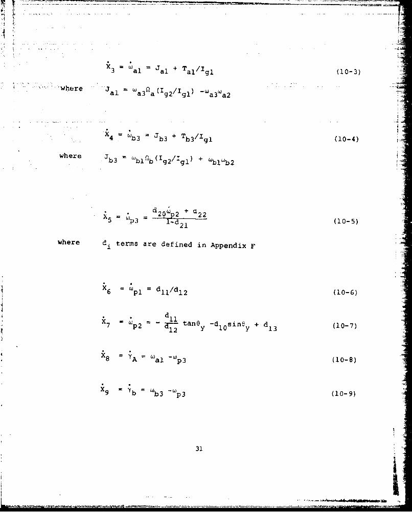
X3 =al Jal + T al/Ig (10-3)

.where al Wa3a (Ig2/Igl) -Wa 3 wa2

4 b3 Jb3 + Tb3/Igl (10-4)

where Wb3 t(bl~lb g2( /lg ) + wblb2

X d20_p2 + 22 -5= 1-d - 21 (10-5)

where d. terms are defined in Appendix F

dll/d (10-6)

dl

"7 =p2 - -2tany -dl 0 sinty + d (10-7)7 p2 12 y 10 y 13 (07

A al -wp3 (10-8)

X9 y b W b3 Wp3 (10-9)

31

klO Ya (10-10)

SXII =~ Yb ( 0 I ):

C11 =(10-11) -i12 •T (10-12) *•=

Te 2w + + W(A -T a (10-13)

The following table shows the source of development of the systemequations

Equation (s) Source

10-1, 10-2 Appendix E

10-3, 10-4 Sect. 5.0 & Appendix A

10-5, 10-6, 10-7 Appendix F

10-8, 10-9 Section 3.0

10-10, 10-11 Equation (9-20)

10-12, 10-13 Equation (8-12)

32

11.0 COMPUTER SIMULATION IThe computer program based on the preceding analysis is-I

described and listed in Appendix H.

11.1 Parametric Values

Parameter values are shown below for two cases. The vari-Aable designation in front of each corresponds to that used in

the computer simulation. 4I

Case 1: Ship rolling and flexing

Case 2: Ship rollibg, pitching and turning at high speed.No flexing included.

Case 1 Case 2

D(1) = Desired Azim (Deg) 0 0 JA

D(2) = Desired Elev (Deg) 57.3 57.3

D(3) = Roll Amplit (Deg) 20.0 20.0

D(4) = Pitch Amplit (Deg) 0 10.0 1D(5) = Flex Amplit (Deg) .5 0

D(6) = Roll Period (Sec) 10.0 10.0

D(7) = Pitch Period (Sec) - 15.0 pU

D(8) = Flex Period (Sec) 1.0 -

D(9) = Roll Height (In) 1200.0 1200.0

D(10) = Velocity (Knots) 0 20.0 ID(ll) = Turn Rate (Deg/Sec) 0 3.0

D(12) = Heel Angle (Deg) 0 0

D(13) = Cant Angle (Deg) 0 0

33

D(14) = WN Train Servo 3. 3 .

(Rad/Sec) 7

D(15) = Damping Ratio .7 .7Train Servo 4

The values below were used in both cases:

E(l) = Platform Mass (Lb-Sec2/In) 0.25

2E(2) = Gyro Mass (Lb-Sec2/In) 0.06

E(3) = Gyro Mass Offset (In) 0.003E(4) =Plat Mass Offset (In) 0.003

A

E(5) = Plat 2 Mass Offset (In) 0.003

E(6) = Plat 3 Mass Offset (In) 0.003

E(7) = Gyro Friction (In-Lb) 0.04

E(8) = Gyro Spring (In-Lb/Rad) 0.20

E(9) = Gyro A Control Gain (In-Lb/Rad) 108.0

E(10) = Gyro B Control Gain (In-Lb/Rad) 108.0

E(11) = Platform Friction (In-Lb) 0.5

E(12) = Platform Spring (In-Lb/Rad) 1.5

E(13) = Gyro Inertia 1 and 3 (Lb-In-Sec2) 0.5

E(14) = Gyro Inertia 2 1.0

E(15) = Platform Inertia 1 40.0

E(16) = Platform Inertia 2 30.0

E(17) = Platform Inertia 3 40.0

E(18) = Gyro Spin Speed (Rad/Sec) 361.0

3I

S341

E (19) Platf Contr Gain (In-Lb/Rad) 50.0

E(20) = Platf Torq Integr Gain (In-Lb/Rad-Sec) 5.0

_E(21) = Gyro A Torque Bias (In-Lb) 0

E(22) = Gyro B Torque Bias (In-Lb) 0

E(23) = Plat Elev Bias Torque (In-Lb) 0

E(24) = Plat Cross Elev Bias (In-Lb) 0

E(25) = Limit on Gyro Torquer (In-Lb) 5.0

E(26) = Gyro Speed Mismatch 0

11.2 Initial State Values

In both cases the system is initialized with the antenna

pointing at the satellite (X1 (0) = Ox(0) = 1. radian;

D(O) = aA 57.30) and with a body rate, w necessary to^ ' p2' sayt

match the £2 component of the ship's roll rate.

Results

Case 1

.Figure 6 shows a plot of the X and Y axis error over a

r period of 75 seconds. The error is the difference between the

computed command angle and the actual angle determined by the

integration process. Figure 7 shows the motion of the 'A' and

'B' gyros about their pivot axes during the same period. There

are two aspects of the response to be examined.

The ±0.5 degree ship flexure input is attenuated to approx-

imately ±0.02 degree of X-Y error by the narrow bandwidth trans-

fer function of the overall system.

The roll input with a 10-second period causes osc'llations

at that period in the X-Y error and the 'A' gyro motion. The 'B'

gyro shows a double frequency response with a 5-second period.

35

L

E TR- 52(6 2 ! -

X76 22:20 80/309 I 1I•e o I I 1 I I I I ! I I I I I 1 -

SHIP ROLL: 1200, 10 SEC PER i- SHIP FLEXURE: t.5', 1 SEC PER

oo ROLL HEIGHT. 100 FEETTRAIN (AZIM) - D 0ELEVATION - 57.3

1 .00 -

.o -- X-AXIS ERROR STEADY STATE

0.

Y-AXIS ERROR-0* 9 - iSTART-UP TRANSIENTIN COMPUTATION ONLY

-.00

-. 0. 0 I I I I . I I 1 I I I I I

0. 10. 20. 30. 0. so0. s0. 70.

Fig. 6. X-Y DMS error (rolling).

36=

Vo

ITR-562(77)1X76 22:20 80/309 2

e.00 I I I1 I I' I ! I 1 ! !

SHIF ROLL: ±200, 10 SEC PERSHIP FLEXURE: ±.5°, 1 SEC PERROLL HEIGHT: 100 FEETTRAIN (AZIM) 0oELEVATION a 57.3

I 00

'A' GYRO STEADY STATE

0.0

0.0J ,... V.

,._J -0.90 -- • -.

z:44" 'B' GYRý

- ' -- :' -

L *I,00•, -e oo

J•0. 10o. 20. 30, 40, so . so . "0.•

T S(C

Fig. 7. X-Y DMS gyro motion (rolling).

37

After an initial transient a steady state response is achievedin approximately 30 seconds with an X-Y error averaging lessthan 0.050. :11

Case 2 H

Figures 8 and 9 show the X-Y errors and the gyro motion overa 90-second period. This is a more confused dynamic environmentthan in Case 1 and, accordingly, we see a more confused responsein Figures 8 and 9.

After an initial transient a general steady state band ofresponse is achieved in approximately 60 seconds with an average

X-Y error of less than 0.1 degree. I

A

-4

38

m ,

____ _ I

I TR-562(8])

X76 22:09 80/339 Ii.0 o-0' I I I | ' 1 I I" I '1 1 1 1 I " | I "

ROLL: t20ok 10 JEC PERPITCH: f20 , 15 SEC PERSPEED: 20 XNRTP.o TURN RATE% • /SEC

- ROLL, PITiH HEIGHT: 100 FEET

I .00•

X-AXIS ERROR

0.50

Y-AXIS ERROR-o.-0

r- I0

-2 .0 oo I ] I I I ] 1i I _I I I I I ~*1 0. 2o r o 0 0 . s0 . 70 o 0. 9o.

Fig. 8. X-Y DMS error (roll, pitch, turn).

39

=I -1

JtTR-562(9)x76 2309 80/339 2

SROLL: 120• 0I0 SEC PER0 PITCH: 110, 15 SEC PER

-SPEED: 20 KNRT$ -TURN RATE: 3 /SEC-ROLL, PITCH HEIGHT: 100 FEET

0.5 01.00I* 'A' GYRO

0. 10 4 .0 0.1

Fi. - 9. X- D yomto rol ictr)

0 ,00

-,.oo "

0. 0O. to, 30. '.0. !0 00 70. 80, 00.

Fig. 9. XYDSgr mton(roll, pitch, turn).

: !

= 40

APPENDIX A

IEULER EQUATIONS FOR GYROS AND PLATFORM ... TI

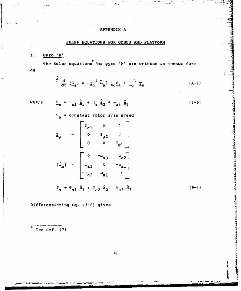
1. Gyro 'A'

The Euler equations for gyro 'A' are written in tensor form

as

A

A Awhere W= a + 2 a,, +w a (3-6) A-a al-i a-2 a3-3A

a = constant rotor spin speed

1 0 01 A

1g 0 Ig2 0

0 0 Igi0

0 12

r0 -a3 a2

[Wa] = a3 0 -W al

L a2 Wal 0

Za T A A Aal S a +T a +T a (9-7)-a aAi 22 a3-A3

Differentiating Eq. (3-6) gives

See Ref. (7)

41

A

ad A ( A

ME a al-Si a3 -3

Combine (A-i), (A-2) and the terms defined above to get

~~t.1i/Ig 0•a -W w.

{al~ - l [/~ g a3 Wa2

g2a3 0 al

a3 L0 i/I 9 a2 w al 0

0 1g2 0 a +

g0 1 a3

i/I gI 0 0 Ta].

0 1/Ig2 0 Ta 2 (A-3)

0 0 i/Ig TaTI a

After some algebra the second of the (A-3) equations vanishes

leaving:

gi a3 a g2 -wa2 a31gl all

1/ [ wl02 + T (A-5)'a3 i/Igl[wa2Oalgj. -al aIg2 a3)

I4S42

which can then be put into the form of Eqs. (5-1) and (5-2)

al - al + Tal/Igl -S-i)

Wa3a 3 3 / (5-2)-- + Ta3/Ig 3

where

Jal a3 (Q aIg2 -a'2Igi)/Igi

Ja 3 'al a g2 a2 gi)/IgI

2. G yro 'B'

The development of Eqs. (5-3) and (5-4) for the 'B' gyrois similar starting with

A

TtE = g(]b + I. ,(A- 6)

3. Platform

The Euler equations for the platform are

i * IP p (~p3~+I -; T (A- 7)

43

i

where W - •pl P1 + Wp2 P-2 + (p3 P3 (3-3)

I pl 0 0p31

A

0 I p2 0 in prame

0 0 I3

F ~"'p30 -Wp Wp

= I )Wp W p3 0 - W pl

L•p2 Wpl 0

T T A +T + T A (9-23)-p pl 1 p2 P2 p33

There are no gyroscopic terms in (A-7) since the platform

motions are relatively slow, therefore expansion of (A-7) leads

to

* A * A * A4) W 2(A-8)

-P pl1 P1 +p 2 P2 + P33

wherel P Tpl/Ipl

p2 p2/p2 (A-9)

p3 p3/p3

Equations (A-9) are Eqs. (6-1) , (6-2) , (6-3).

44

I

APPENDIX B

CONSTRAINTS

The angular velocities of the {a"} and {b} frames are con-

strained to that of the {A} frame by the gimbal arrangement

shown in Figure 3.A A

Consider the {a} frame which pivots about a The compo- A- 4-l

nent Wal is not constrained; however, w a2 and wa3 re by the

equality of the vector sums:

A A A A (-Wa2 a2 +wa3 a3 w.2 P2 + wp3 P3

Using the relations defined in Section 2.0 we can write

S= [C l(Ya)] j}

1 0 0 0 0F cOSY siny a p2 cosy a + Wp3SinYa (B-2)

a aOY p2 in" + wp2sCOYaS -sinY cSY p3A p2 a 2

C- 2)a a

Combi.ning (B-1) and (B-2) we get the equations

45

Wa2 (p2Cos a + 3siy (B-3)

•a3 = -p 2S inya + wp3COSYa (B-4)

Equations (B-3) and (B-4) are Eqs. (7-1) and (7-2). SimilarlyA

for frame {b} which has a single degree of freedom with respect

tO {P} about axis b 3 we get

A AW bl -l + t22 - pl P1 + 'p2 P2 (B-5)

Ab} [C3 Cyb)] (P-)

OSY sinYb 0 WWplCOS'Y + W sinYb

F bnY OSb o l P1 b +p 2 b1 BCLs~nYb cosy0 10 W~20 -WplinYb + (0p2COSYb (B-6)

bS b 2 l p 2 OS b$

Wbl = pi CoSYb + W p 2SinYb (B-7)

Wb2 1 plSinYb + Wp2 CoSyb (B-8)

Equations (B-7) and (B-8) are Eqs. (7-3) and (7-4).

46

LiL

*. . ... *

APPENDIX C

TRANSFORMATIONS FOR e AND 0 _

- xc' yc _4ýj O

In this appendix we expand Eq. (8-8) and solve the results

fore and 8-xc yc

0 0T T T1 2 3 (8-8)

The unknowns x and 0yc are contained in B2 and so we premulti-xc ycply by B1 to get

T 1 BT 1 (C-l)B2 0 B1B3 0

Expand the left side

B2T [C(a)]T [c 3 (ey)]T 1

47i; ~4 7 ,

e;

__ - -=~ - __ - ' ~ - ~ -- = ~ -- -

o cose IcsnyBT 1 0 cose -sine sinO cos0 1

V o:e cose :] (C-2) 71.0 0i80 cos 0 0

-sinyo

Expand the right side of (C-i)

I00 T 4

AB B= [C3(eT I [C2(,H [C (,p ][C (,a ] [C (.A ] a )T 1

0 0

&; = t2 (C-3) :

t3

'33

The ti terms will be determined by numerical computation ofS~(C-3). Then equate the first and third components of (C-2) and( iA

( -3) (48

t3 A' -

-iS ' • " ' I • • I • • • -- -- - •'=•- • " • . ..

St : m .A__ .. . .. . . -- . .---

-sine y

t =sine Cos6 .--.

a--3 xcC° 'c 71

"JASolve for 6yc and 6 ".

yc sin-i (_ti) •2

Oyc xc

Sn t)(C-4)

xc sin- (t 3 /cosayc

r

49-

APPENDIX D

ACCELERATION VECTOR & TORQUE DUE TO UNBALANCE

We consider accelerations due to the following sources:

azea) Roll (horizontal component along •)

A [c) Gravity (vertical along n•)

AId) Turn (horizontal component along )ii

1. Roll Acceleration (horizontal component along ni)

-R Il (D-1i

H = roll height JH

WR= roll frequency

•RO = roll amplitude

2. Pitch Acceleration (horizontal component along n2)

= HPA, (D-2)

p p 22

50 •I:

2where = -W 2p sinw tp P PO p

W P = pitch frequency

'4'pO = pitch amplitude

3. Gravity (along n3)

A = 386 in/sec2 n• (D-3)

Note on Polarity of A :-.g

Force due to gravity acts down at the center ofmass. Its corresponding support force at thepivot axis is positive in the upward direction.Torque about the mass center results when the LIline of the positive support force does not pass

through the mass center.

4. Turn (horizontal component along n•)

aT =V WT (D-4)

where

V = velocity A

WT = turn rate

51

A

I

5. Total Acceleration in {n')

We add components above to obtain I

Ai A3 +A A niiA~ lj -A3 (D-5)

where A= H R-V WT

A= H pi

A' = 386

6. Transform Acceleration Vector to {}We transform from {n') to {p} usingI.

{A1 [C3 () ] [Cc(0)] ][(T [C2(pR)] A[CI(* _n (D-6)

and define the resulting components in {•} by

A A A I

Az A 1 1 + A2 P 2 + A3 E3 (D-7)

7. Unbalance Torque

Unbalance torque due to the combined effect of acceleration

and displacement berween the centers of support and mass isdefined by the cross product:

52 Ii

II|

--- (-- 8) ~~~

L F x R

where L unbalance torque vector

F - force vector at support point

position vector from support point to mass center

The force vector, F, is due to the effect of gravity andacceleration acting on the mass.

F m A (D-9)

8. 'A' Gyro Unbalance Torque

Transform A in Eq. (D-7) from {•} to {•) coordinates using

A (A(D-10)

•41 0 0 A 1A1AA 0 COSYa sn JA AOS + A3Binla (D-11)

0 -sinya COSyaJL3 -A2 sinya + A3 COSYa A

Write the result of (D-ll) as

A A A

A ,ýl Ia2 12 1a3 a3 (D-l12)

53

: !L °-' •- • •------ • '-•'-2-- • • • _• - - , __ -- -- -_ • • • . I•' - %

where a 2 - A2 COSYa + A3 sinYa

a -A 2 sinY + A3 COSYa

Now consider

R= 2. _- g 2

A A AF m A =m(A. a + a a + aa)1 -i '2 2 3-23

where 9g displacement of mass center from support point

m = gyro mass

A Athen T = F x R mg (A 1 -3 -a 3 -l) (D-13)--au -- 1ýý -- 3 gAl

The a component in (D-13) is an insignificant bearing reaction

torque which can be neglected. Therefore using the definitionof a 3 in (D-12) we can write

--au -mkg -A 2 sinYa + A3cosya) (D-14)

9. 'B' Gyro Unbalance Torque

Transform A in Eq. (D-7) from {p) to using

(b) [c3(-Yb)]1 2• (D-15)

54

I i

rcosy sinYb 0J A A ACOSYb+ A2 siflY

Soib .nb 1, a.o.b 2 ,,nb{A - sinYb coSYb 0 -AlsinY A cosy (D-16)

L b 2. bA 3I

Write the result of (D-16) in {b) coordinates as -

A A AA= bI bl + b 2 b2 + A3 b 3 (D-17)

INow consider

Ak A A

F - m A -m (bI !aI b 2 t2 + A3 !13)

I

Then Tb F [x R =t m(-bl -•3 + A3 bl) (D-16)

^4A

We neglect the bI component following the same logic that pre-

ceded Eq. (D-14). Then use the definition of bI in Eq. (D-17)to obtain

Tbu- - m g(Al COSb + A 2sinb) (D-19)

55i

10. Platform Unbalance Torque

Here we model unbalance about all three axes by defining

R~L A A A

R 1l21l 2 22 +3 23

now

A A A A A :

T = F x R =M(AP1 + A2 P 2 + A3P 3 ) x (£ipi + k222 + z3P3)

A A ATu TT + T (D- 20)T Tpul 21 Tu2 22 Tu 3 23

where

T. M(A2_3 - A3. ) k

Tu 2 = M(A3 1Z A Z3)

u3 M(A 2 -2

M = platform mass

56

APPENDIX E I

GENERATION OF SYSTEM EQUATIONS (10-1) AND (10-2) FOR 6AND 0x y

1. Approach

System equations (10-1) and (10-2) are integrated to provide

6 x and 6 position data. In the real system 6 and 0 would be !y x y

the output of the synchros on those axes.

The solution for 0x and y is obtained by using two of thethree scalar equations in the vector equation (3-4) H

W + 0+' (3-4)-p~ e! x91 y 23

ii

The process is one of defining _wf, putting all components of

(3-4) into a common frame {p} and solving for 8 and 6 asx y

functions of w fi' 0T' ex and ey. j2. Generate wfi Components ,

First generate the wfi components in Eq. (3-1) H

fI

A A Af f wf +W f (3-1)--f = fl - + ff2 2 f3f3 3

by making use of Eq. (3-2)

+ ! + Ii (3-2) -A

57

Transform n n into {n"} using from Section 2.0 1

[C Ar I] In

11 0 0 0 (0

I-0 Cosp sin'p 0 sin4p (E-1)

P p A',~ AC 'p I0 -sinp p Cos*p •A ýAC°Sý p A,

ANext add 'P n" to (E-l) and transform to {f} using fromSp_ -1Section 2.0

{A }= [C2(R)I {n"} n

R R -

0 1 0 A sin(p PAsintp - s(E 2)

sinPR 0 cos1RJ CSp , SinR + C°SC c A

Finally add to the result of (E-2) to complete the deter-R =2 A

mination of the {f} components of wf

58

A

W fl •pCOSý R _•Asin.lRCOBS p

= + IAsinp (E-3)

tf3 = tpsinR + &ACOso RCOSý p

3. Transform (3-4) into A Coordinates

Now proceed to transform all components of Eq. (3-4) into

the {p' frame.A

Transform wfi in Eq. (E-3) into {f'} using from Section 2.0

A {A

(f,} = [c 3 ( T) f}

cosT sine -0 f cose T+ W sine TT T f2 fl T 2

[Linj cose A ~wflie +w3oe~ E- f3

A ANext add T f to the result of Eq. (E-4) and transform into {•}

T-using from Section 2.0

We facilitate this by defining the first two terms in Eq. (E-4)

59- _

I= Wflcos T + Wf 2sinlT

D . . D2 s= flsinlT + wf2coseT (E-5)

Then

0 cosex sine D2 = 2cOSex+( T+Wf3)sinex (E-6)S-sine ji wf 3 +T D 2 sx+(T+ )cose.- f , 21.2j AD s n e ( T + w 'A

A ANext add 0x 91 to the result of Eq. (E-6) and transform into {•}using from Section 2.0 1

iiFirst redefine the last two terms in (E-6) as i

Y2 = D2 cosox + (0T + Wf3 )sinex

3 2 -D 2 sine + + f 3 )COSO (E-7)

Then

60

FCosaY ySing U e (D1 +8x)CosG y+y2 sin6sin6 cose8 y2 { -(Oi )sin5 2 cosO (E-8)

L3 Y3 A

Finally add 6Y to. te result of (E-8) to get 51

.. •pl = (DI+ x)CosOy + Y2 sin6~ - - - - 12= -(D 1 +6 x )sin8y + y 2 cosO (E-9)

WIP3 -- y•

4. Solution for ex ey

Now solve directly for 6 and 0 using the third and first 4x yof Eq. (E-9) ,

ey p~3 -y 3(E-10) 1

( Wpl - DlCOS6y - Y2 sin6 )/Cosa e

These are system equations (10-1) and (10-2). It is signif-icant to note that these equations for 8 and 0 are functions ofy x(pl p3' 0T' Wfl' Wf 2 ' Wf3' 8x and 8T' Notice that wp2 does notenter these calculations. We make use of this fact in Appendix G.

A

61

APPENDIX FI

GENERATION OF SYSTEM EQUATIONS (10-5), (10-6) AND (10-7)FORw -p3 I

ý-ORpV3-ýpl--4 2

1. Overview of Process

Considerable algebra is involved in obtaining Eqs. (10-5) and

(10-6) due to the need to eliminate unknown bearing reaction

torques Ta 3 , Tbl, TpG. The Euler equations (6-2) and (6-3) are

the starting points with additional relations coming from the con-straint equations in Section 7.0. A number of transformations are

required to obtain scalar equations in a common frame.

Specific steps in the process are:

a) Differentiate constraint Eqs. (7-2) and (7-3) to obtain

new equations for (-a and w

b) Combine results of step a) with gyro Euler Eqs. (5-2) and

(5-3) to define reaction torques Ta 3 and Tbl.A

c) Perform transformations to define E components of totaltorque T in Eq. (9-22).

-pd) Introduce T components from step c) into platform Euler

equations in Section 6.0, then use results of step b) to eliminate

Ta 3 and T

e) Use wp2 as defined from velocity constraints in Appendix

G to eliminate T leaving equations for w and wpG p3 p1*

2. Differentiate Constraint Equations

Differentiate constraint Eqs. (7-2) and (7-3) to obtain new

equations for a3 and

62

_~~ -W' ....... . ... .. .. L_• _ - _-. ....* - •a3 p-2S 7a + wp3CoSy .a (7-2)

[ ~~l-W uW COSY~ + Wsn•::• : •z• • • bl 1 •p C S b + p 2 Si n b (7- 3) i

-- Then

siny + cosy + Ua3 p2 a p3 a a3

Wbl PI copC°Syb + Wp2 Sinyb + Uh, (F-2)

where

a3 -wp 2 COsya - Wp3Yasiriya

UbJ = -WlYbsinY + WJp2 YbCOSYb

?, Define Ta 3 and Tbl

From the Euler equations in Section 5.0

a3 Ja3 + T a3/1g3 (5-2)

Wbl "bJbl + Tbl/Igl (5-3)

Use (F-i), (F-2), (5-2), (5-3) to eliminate •a3 and wbl anddefine Ta3 and Tbl

1 63

S": : _p Sinya p COSYa +.. .. -3r Ta 3 = g 3 + a+ Ua3 - a3(F-3)

Tbl = Igi( WplCOSYb + Wp2 SinYb + Ubi - Jbl] (F-4) I

4. Platform Torque in {P} coordinates

Next express

A AA

Tp P + p22+ p3 3(F

for use in the platform Euler equations, Section 6.0.

Start with Eq. (9-22) for T and identify the components

in that equation from Section 9.0. 111

-p -ps + -pF + -pu --TpB + !R -Pc + Z p G 9-22

Tp = -1s p[ 8 x gl + xy 231 (9215)

A

; pF = -KFp[{6x/IgxI}-gl + {%y/Il} 2.31 (9-16)T A (9Pl1 /16 P (9-16)

-Pu p x X -

T-pu= T Ul T u2 P2+T u3 P3(-7

A A

TpB TB l T (9-18)

64

-G =-TG (9-19)

A A AT = p a + al --aB3) -K (fyb dtp + fYadt P3 (9-20)

-:-PC

rT =p al 22 (9-2s1)E. 9-)

Rerte Eq (9-22 as+T3b se q 91)

A A

REwrit Eq.6 (9-22 as • fae

1 t o1 (Ta lb p 1 -6)

where

T -K 6 1( K~ ' 6 + T~ ~KCYb ~K ~dt

3 SP sy KFp fey/IyI} By KPC a KpiJ*ad

A AT T al 21 + T a3 13 (see Eq. (-7)

A A

TEb T Tbl hl + T b3 b3 (see Eq. (9-14))

Now start a series of transformations to put all components of

Eq. (F-6) into the {A, frame.A -T A {A

First transform Ta -T Ta a, Ta3 -a3 into P.using, fromSection 2.0 a

65

C . • , - .. " ' -• • " • •' • •"••- : • •

{A} =C ]T[2IA)

1. 0 0 - T al -a

cOSya sfinYa T Taina (F-7)o ila CSaja3 a)"0 sin coy -. T OIsna cSa \-a3 A -a3C°Sa -

SectiontoA{} using from A

Next transform Tb = -Tbl bb into -ui frSection 2.0A

{) _- [c 3 (Yb)bT{b}

°SYb-sinYb ]-T -Tbi COSYb)

rinb cosy 0, 0b -T 1 n (F-8)

-T~ A -Tb A

A ANext transform T1 g+ TpG g2 into {; using from Section 2.0

{•} = re 3 ()] {• 6

66

7T

Cos8 sine 0 T1 o 6c°SeY +T inyi' y Y Y pGsiny

s COs0 T -T s + TpGCOSBy (F-9)NOi cy :y ] pG isin7 Ay• • .0 0 1 0 ^ ..1=54

NOW sum all of the {p} components in (F-7), (F-8), (F-9) withT3 23 in (F-6) and Tpu as defined in (9-17) to obtain the T

components in (F-5).

iTpl = -Tal -T blCOSb + TlCOBy + T pGsine + T-

pG y Tul

Tp 2 = Ta3 sinya -TblsinYb -Tlsin6y T + TpGCOY+ Tu2 (F-10)

Tp3 = -Ta3COSYa -Tb 3 + T3 + Tu3

5. Put Terms into Euler Equations

At this point combine the definitions of Ta 3 and Tbl in(F-3) and (F-4) with the {p} coordinates of T in (F-10) into

the platform Euler equations in Section 6.0.

The Euler equations are:

•pl =pl/Ipl(6i

- •p2 = T p2 /Ip2 (6-2)

"4p3 = Tp3/Ip 3 (6-3)

67

Z

--- -. --- -

Using Eqs. (F-3) and (F-4) write Ta 3 and Tbl as

a3 r 2 r 22p 3 + 3

Tbl s 1 •p 1 + S 2 p 2 + s 3 (F-12)

where

r = -Ig3SinYa s =glOSb

r2 = Ig3 cosa S 2 = Iglsinyb

r 3 = Ig3 (Ua 3 -Ja 3 ) s3 = Igl (Ubl -Jbl)

Use (F-lI) and (F-12) to eliminate Ta 3 and Tbl in Eq. (r-10) and

substitute the result into Eqs. (6-1), (6-2), (6-3). 11II

pl= -Tal -cosYb(Sllpl + S 2 ip 2 + s3)

+ T1 cosOy + T u + TpGsiney (F-13)

p2 Wp2 siny a(r Ip2 + r2 p3 + rj3)

sin.Yb(Sl pl + S2%p2 + s3)

T sin3y r + T cOSy (F-14)

r'¢ 68- ~ + .. cos

m m m m , m• : -"y

Ip3WP3 = -cosy a(r 1w + r 2Wp3 + r13) -T1b3 + T3 + Tu3a p3 p2 2p r) T 3 + +(F-15) q

6. Elimination of and Solutions

Eliminate Tp by combining Eqs. (F-13) and (F-14) to obtain:

pld5 p2d 6 p3 d 7 =d 8 ....P3 7 8(F-16)

I Awhere d 5 1ssinyb tansy -Ip, -SlCOSYb

d6 = (s 2 sinYb -r sinya + Ip2) tanf2) y -62cOSYb

d7= - r 2sinya tany

y uI

d 8 =Ta + s3cosYb csi.Tu-

+ (r 3 siny a -s 3 sinrb -Tlsin6y + Tu 2 ) tanbSuy

Write Eq. (F-15) as:

4d320 p2 d 2 1~ d 22

d 2 p3 + (F-17)

where d 2 0 = -(rlcosYa/Ip 3

d21= -(r 2cosYa)/Ip3

d 2 2 = (a-r 3c°SY -Tb 3 + 3+ Tu3 )/Ip3

F p969

This leaves two equations ((F-16) and (F-17)) in three

unknowns, wp11 Wp2i p3" Obtain a third equation from the

velocity constraints due to the gimballing that is determined

in Appendix G. The result is:

-- ~- taney -dl sine +(G3

p2 p1 y 10 s y d 1 3 (G-3)

where d1 0 and d 1 3 are defined in Appendix G

The solution of this set of equations ((F-16), (F-17)),

(G-3) is:

dp 1

2 - 1tany -d 0 siny + d1 3 (F-19)12

d (F-20)3 -212

dd20 .dd 2 2 )where d1 =pd8 + (d 1 3 -dl siney)(-d 6 - 7-202702212

7d2d20"2

d 1 2 d5 + 6 - 21

70

I-

APPENDIX G

GENERATION OF FROM VELOCITY CONSTRAINTS

This appendix develops w from velocity constraintsp2

imposed by the gimballing configuration for use in Appendix F

as the third of the three platform system equations.

The process here is to use Eq. (E-9) for w and differen-p2 -tiate. Additional relations are obtained from Appendix E, noting

that e and 0 are independent of wp2 as indicated by Eq. (E-10).x y p

= -(Di + )sin + y2cose (E-9)

where D1I WflcoseT + wf 2 sineT

D = _-flsineT + Wf2coseTO

Y2 D Dc°S + + wf 3 )sinEx1

Differentiating Eq. (E-9) produces

p2 -(D 1 + ex)siny -%y (D 1 + ex)cosy

+ Y2 cosey -y 2 ,ysine (3-l)

71

We now require relations for 8x, DI" y2 " From Appendix E,

Eq. (E-10)

;x = (Wpi -D1 C°ey -D -sine )/Cosy (E-0) I

Differentiating Eq. (E-12) produces

o= + d <G-2)x cose 10y

where

d (-Dlcos0y + Diey sin -0 cose10 lY sny yy y

(cos 1 + 8y(W•p -DlcosO7 -Y 2 siney)

cos- 2 siney y

Substitute Eq. (G-2) into (G-1) to obtain the solution

= -W tany -d sine + d13 (G-3)p2 p1 y 10 y 1

where d = -Dsin -(D + )COS13 y y 1 ycC5

+ 2 cose y -Y2y sinOy

72

-4--

"-We define DV D2 and 2 by differentiating the equations under(E-9) above:

D = CoSO -w + sine + + wf2 TCoSOT (G-4)1 fi T fi T T wf2slnOT f

S D2 -wfsineT -wflleosaT + •fcoseT -wf6 sineT (G-5)

2= DDCOSx -D 2 Csine

+(a + )sine + + wf )csx (G-6)

ins Appndi E.n Coq c;•col

* C:

--Dcose -D sine -sncs . c o

+ ApSinýRsinýp (G-7) !4

+f2 = iR + COOsinp + ApC° +fp (G-)

in Appendix E

S= sinR + 'pRcos'PR + IAco°sRC°SOsp

-PAIRsinIPRcos'p-4 'PA cosl sin'p (G-9)

73 iI!

APPENDIX H

COMPUTER PROGRAMS

INTRODUCTION

The Fortran computer programs contain the inputs, torques

and system equations defined in this report and computes the

system trajectory by use of Runge Kutta integration.

PROGRAMS AND SUBROUTINES

MT21D: Main program

MTRKI: 4-cycle Runge Kutta integration

MT22: Ship motion and coordinate transformationfor command inputs

MTl9B: Torques

MT20B: State equations

PLOT: Library plotting routine

Figure H-1 is an overall block representation of the program.

The listing of the program is attached.

LI

74

n n I j | | | j JI

TR-562(H-I )I

MTRK 1

MT 22MT 19BMT 20B

D )CISION

STORE FORPLOTT ING

Fig. H-I. Computer flow diagram.

75

-lag"

Sheet I of 5 A

_:A0 a'9

Q9

0*0cto%:: a4;M 0;

4*40 ItA u M x r9 a

2 LAG; '!4; 0.1- a L, 9 0 X 91-M ox 'iic; : ý';w - .9 1.- V 19

3fý;. - U a x a z 0,; It Qt.600 x :11 -_'.ýMvw son I .,a j 'i x

61, :1 IL a X xaftNO-JMW 000 0 IL 0 60 It 1;

MWAA z.Z..To 61 a. 61 z m IOc- -Ulm Mo c t "

I cau; k . 6..4 Jim 0 a 0'. 'Am O'X ! a It: .*", . -!a'!- rw. Ow

zlox, I* rj Vt- .61a- %a0;;ac.w v4; Z we Opal-IL ::"j I ý17 eels a __Ato_ý ý.Jýtx

alwtw!c 4 a b- b.. I., ý '; a -so-)X zcic.ý; *3

U X Z qc -I qw 0. 11 na ý fto ;.Zoo 0 '2 W. :'J z -1 a 4 0 .'L 0MO . a log log .9 1.9 wo 0 a a 3 3%L 3'L ut

a 1A A 3

IM

Oxtwý' ado 40 0 > 9- 0 0 Z

- 0.. a z Xýu

Ir i Z; - - - . FCZEW 0 M -1 1- 1-. IL 0

rn _4vz w a x Xý'dc z c I4, 4L & a ..3 Z z T a'j 0, V, M 1 s

cc

fid 0 Z - - ;;;:.Z X,Ok - - 18 MO. 0T;: xxxxxxx coopuaaa 030 12-

:00I) ;! X: 60100%

4 L

6M 0 -6 C-z= 0 'M a 0';ý; W6132;; ;;Ooo;;0 W ! ý L, ý - 6 ! ; ; ! ; a a

100

'AwA O!wg!.Jooww

0 dw-.4ft 4.1w __ -- !Zzm 0

-0- *4 ýZzc_ saw ccuot.4_J "

a c a - 0 0 1- D_ 1w

4L amezz a WO 0 zw

1:1:w :01-alak .49 O.W K'LL Ole L'ýýfAq iýA. 1-6w%ýL sk46 x 1ý. a 0. $_ . , ":L' - 1ý @_ $_ $_ 0 ý ý 0 0 a I.- 1-. 0 0 0 P.

!,Sze a ww.. 1. :! Xw 6-00445000T!ew N

0"_ I Z 2 1126 a -Z a t C. too L =icm maul's a 7 ft. a 000

C\i 7M , V ::7.;;

Oft Ic a 0- 0 xxxx x K 000000a 0004- z

0 0 U 0 Q 0 0 Q 0 U 0 W 0 U Q W 44 V W Q U 0 to V W 0 0 W W W V U IJ V 0 0 U 0 U 0 0 w CAU 0 0 0 U tj Q

76

-Sheet 2 of 5

1* .4W-1I

lei I"V2 01~ ~40

7f ;* a

0 b a z Zjt-z I 0 . .-r

WO . - I4 'AI* &l

af a .- at .0 04 i 1

X,. 03- In o m*p jabVa ti !d0 via ja -i I.. 8

Vn Lft41*u U -w I.-4j; 4Di0f w PEW

U#~S*Z* 8-*~~ ~I!I AiI: I~fI!I!!I',., ,*~ s-rn.. i .s

~be-~ 5 -gw*4-.- ~ ao., .- ,..u... a',..) 0M2

pa.

li 1. W- za

t. 9- a i

Ii It-W - !a ~ ~ -0 Ugw - : . ;

U_ V. D- 2'0 P31V 0 o uIL

ImaLP* 8.0 uwL"Q u

sheet 3 of 5

JI'iA

6!4

Uc 0

s-'-I - - -U ..

.- ~~~ F- Or. a a.- W-- *-0 -.-0~4 0 .~-

0 W-5Za- 0 -651 3 a, (

ck. M--! I I~a~~* -aux0 4s

"A- h 2Ww IA 0A5 4 5 a t. S . *

r -s ..-- i .. u w a 01

54 !;OnA OS X34- RS 65.4 a, x* *war- a. W. -A a .U*U -

024 0.J at-- a w ua M il t- T a a C;.0- S I

a 0 a 1. 6 1

IA

- -. 0 0

,2I a al It av 40 :. 40 0 n up

1 Lao 1 ,u to 0.

-M( 'S sa,: F U~f

X% 00 65.5 a

a a0-$-eFMW Zm I.-g- a- ---- w-0 f0- *~'5 as emo ,a ,: 0 .a a0

400

*~ -5.

usa li U 4_.Q *Uv L uw Uw

Sheet 4 of 5

+_+It t -3*10;. :. ==1

DMoX_ Al du 2• --- ...

x,, ;-,+ = _-.?y - - .o -y to Q ,, 0' --NA* -0 - a a-

33 .. . N -" am -..

"" N Ou - ;"G- - -==-' -- la" U x

00 2 fq

IOU X ;'' 1a

sag.4 I.N y-- N. NN"U

-9 aNN Ux M, x' w ." ax 4.

0N x A I-. .. A -;K2:94 N : - Nm U z; 0 w 2--

-I• IIk , - IA -. -- 1 EUU O%-Ii * 2' M1 N.l2lx I IA-. N-• ). *-MN X--'( - e C • I -II0 0 091

xI I a z 0 -a i i Ii A K I .

' N.. U 'N'I • I° A NU .I • -.~...a O- W IA. AhI ... ..... o-°' a1 - £+ azwIIl'S. -N .N - I P1- IA N I --Jww E- . E '- -. I a aJUMUU a o -- -- ~v O--+ - Iuao -- +° 'O+ -N |

D. 0010

m II

N l •e - 0 l ,- . u .a u . - e ~ - , e . - ~ o z

T * l A.a :; - . o as

*4D99~ ~~ x.fP a. &a C6 N -U II - ~~.. a- N N NN W.h,-i 2-

aa tv

Id a -

I- P.q 0 ----

3z~~~~1 N .- " : ::; I;;;; c0 W n0 P

I a a..-0- -WM- 4a fIL a. I.-

-j I I- - -ml W, £I 2 : 0 ,

N ~~~w NNCO- ---

au- m4j a u 0 '

~C'. - Et419

r T T.... -: ••• --- _ ._=f_ L -•

Sheet 5 of 5

z~o

~ -.... ____ __

hi-

-on

40U

.

Poo- a~ 0 - M-)40K - ... .. . ..

S...

" ", • ZS Z..• .,K -U

j•- '.* * .* .11 O

80

•

V=

5 i -

i -

REFERENCES

1. J.B. Scarborough, The Gyroscope (Interscience, New York,1958).

2. R.L. Williams, "Shipboard Stabilization of Optical Systems",Masters Thesis, Naval Postgraduate School, Monterey, CA.(1978).

3. A.H. Bieser, "Combination Gyro and Pendulum Weight PassiveAntenna Platform Stabilization System", U.S. Patent No.4,020,491.

4. A.H. Bieser, "Combination Gyro and Pendulum WeightStabilized Platform Antenna System", U.S. Patent No.3,893,123.

5. R.J. Matthews, "Direct Mechanical Stabilization of MobileMicrowave Antennas", AIAA 8th Comms. Sat. Sys. Conf.,Orlando, FL, 21 April 1980.

6. J.N. Leavitt, "A Stable Platform for Remote Sensing",Can. Aeronaut. Space J. 17, 435 (1971).

7. L. Meirovitch, Methods of Analytic Dynamics (McGraw-Hill,New York, 1980), p. 140.

8. M. Taylor, private communication.

81

NOMENCLATURE

A = total linear acceleration vector (App. 0))AA = i components of A

A = acceleration term due to gravity

A = fore-aft acceleration--p

AR = athwartship acceleration

A centripetal acceleration due to turnF = force applied to platform at support point (App. D)

height above center of roll

I = gyro inertia diadic

a nd i principal inertias of I

SI = platform inertia diadic

pi pi principal inertias of IpK = control gain on 'A' gyro for Y axis errorK b control gain on 'B' gyro for X axis error- JK FG gyro friction torque magnitudeKFp platform friction torque magnitude

pc controller gain for X and Y axis torquers

KpI =integrator control gain for X and Y axis torquers

KSG gyro spring gradient

SKSp platform spring gradient

L = torque vector due to unbalance

() denotes a vector

subscript i applies to all itteqers except for d.

82

Sdispla:ement between center of support and mass for gyro Iz. = displacement between center of support and mass for

platform along pi A

M = mass of stabilized platform assembly ms n

m = mass of gyro rotor and motor assembly

.. It = position vector from support point to mass center

t = time

T- total torque vector action on 'A' gyro

T ai =a. components of T~a

T bias torque vector acting on 'A' gyro

T magnitude of TaB

TaF friction torque acting on 'A' gyro

TaS = spring torque acting on 'A' gyro

Tau unbalance torque acting on 'A' gyro

= total torque vector acting on 'B' gyroA

Tbi = b. components of T

T bias torque acting on 'B' gyro-bB=friction torque acting on 'B' gyro

spring torque acting on 'B' gyro

-bST = unbalance torque acting on 'b' gyroTrbu

TBN = x component of bias torque acting on platform

T y component of bias torque acting on platformByT = control torque applied to 'A' gyroS-c a

T = control torque applied to 'B' gyro

83

T = torque vector acting on platform

ATi components of T

T pB = bias torque vector acting on platform

T c = control torque acting on platform

Tp friction torque acting on platform

gimbal bearing reaction torque on platform

TpG = magnitude of TpG

TpS = spring torque acting on platform

T = unbalance tcrque acting on platform-pu rqo

TR = pivot bearing reaction torque on 'A' gyroTb = pivot bearing reaction torque on 'B' gyro

T. = AT ui = pi components of T

V = ship's speed

GREEK LETTERS

Cc = satellite azimuth ephemeris

a = satellite elevation ephemerisA,

Ya = {a} frame rotation angle with respect to {•}

Yb 1{b frame rotation angle with respect to f}

PA = ship's azimuth

•H heel angle of deck

'p -- pitch angle of deckp

Op = amplitude of harmonic pitch motion

4R = roll angle of deck

84

tP = '1R + tH

amplitude of harmonic roll motion - -- .Ro

) = ship flexure angle I

a = train axis angular displacement

"e = X axis angular displacement

0 = command value for 0xc x

O = Y axis angular displacement

"" = command value for e yyc y

- a angular velocity of {a} frame .1A3

w ai = ai components of w a

b = angular velocity of {b} frameA

wbi 0 components ofwb

af = angular velocity of local deck frame { IA

Lifi= fi components of wf

n = natural frequency of train axis controller

= angular velocity of {•}

wp P frequency of ship's pitching motion

i =pi components of w

WR = frequency of ship's rolling motion

= = rate of change of ship's heading

"Q-a angular velocity of 'A' rotor

= constant 'A' rotor spin speed

2b =angular velocity of 'B' rotor

= constant 'B' rotor spin speed"'b

- train axis contro. damping factor

85 1

TERMS IN SOLUTIONS

TERM WHERE DEFINED

d. (i = 5,6,7,8,11,12,20,21,22). . . Appendix F.61

d. (i 10,13)........................Appendix G

Di.. ... ....................... Appendix E

Jai..... . ........... Section 5.0

J.. .............. Section 5.0

ri ................. Appendix S.F

Si.. . . ............ ...... ... ... Appendix F.5

t ................. Appendix C

Ua3a ................ Appendix F.2

Ubl.................Appendix F.2

Y.i .............. Appendix E

86

-'1

UNCLASSIFIED- SECURITY CLASI4FICATION OF THIS PAGE (Whoen D0l.. £ceredjelf)

READ INSTRUCTIONSREPORT DOCUMENTATION PAGE BEFORE COMPLETING FORM-

I. REPORT4iU.ALL. GOVT ACCESSION NO. 3. RECIPIENT'S CATALOG NUMBER

4- TITLE adS .,is"14J) S 5. TYPE OF REPORT & PERIOD COVERED

Analysis of Direct Mechanical StabilizationPlatform for Antenna Stabilization and Control 2 Technical RepOrt

in a Shipboard Environment 6, PERFOR•MING ORG. REPORT NUMBER

.. Technical Report 5627. AUTHOR() II. CONTRACT OR GRANT NUUMBERt/)

"!iarvin,7aylor F19628-80-C-'0002

- 9. PERFORMING ORGANIZATION NAME AND ADDRESS 10. PROGRAM ELEMFNT, PROJECT, TASK'

Lincoln Laboratory, M. I.T.,r AREA & WORK UNIT NUMBERSP.O. Box 73 Program Element No. 33109N':

Lexington, MA 02173

II. CCNTROLLING OFFICE NAME AND ADDRESS 12. REPORT DATE

Naval Electronic Systems Command -

Department of the Navy 2..

Washington, DC 20360 - 1 - 3. NUMBER OF PAGES94

14. MONITORING AGENCY NAME & ADDRES (if diffe/ren froas CoelvaOling Office) IS. SECURITY CLASS. -o/ ,h reporlJ

Electronic Systems Division UnclassifiedHanscom AFB i _-__ ____

Bedford, MA 01731 IS,. DECLASSIFICATION DOONGRAOINGSCHEDULE

16. DISTRIBUTION STAI EMENT (of ISh Report)

Approved for public release; distribution unlimited.

V=17. DISTRIBUTION STATEMENT I~f the ib roet t .eveied ,in Block 20, if diff-rer, front Repoarl

It. SUPPLEMENTARY NOTES

None

19. KEY WORDS (Contnue on reterse side if necessar.y and erdel/y by block naumber)

stabilization mechanical controlgyroscopic stabilization control

0. ABSTRACT (Coninui, on reverse side if neceizr" and identify by block nutmbet)

This report presents a rigid body analysis of the dynamics of a shlpboard antenna in a three-axisgimbal configuration utilizing Direct Mecha.nical Stabilization (DMS) for primary control. Sys.tem pa-rameters are defined and Euler equations app ied to obtain a non-linear system model that includesexpected torque input,;. A computer simulation is generated with ship input motions due to roll, pitch,turn and flexure and a numerical Integration proccdtire Is then employed to determine the motion ofthe antenna and the resulting pointing error for various scenarios.

The results of the cases studied Iidicate potential feasibility of this approach for applications re-quiring pointiog accuracy of approxhiately U0. 15 degree.

FORM 1473 EDITION OF 1 NOV 65 IS OBSOLETEDDI jAN 21 UNCLASSIFIED

SECURITY CLASSIFICA1ION OF THIS PAGE (lhen Dita Entered;